EXHIBIT 9-6 Comparison of Alternative Inventory-Costing Systems

$30.502.001.00

$33.50$1,200

Actual Costing Normal Costing Standard Costing

Variable Actual prices x Actual Actual prices x Actual Standard prices x StandardDirect quantity of inputs quantity of inputs quantity of inputs

'" Manufacturing used used allowed for actuale.'" Cost output achieved~"u Variable Actual variable overhead Budgeted variable Standard variable overhead":c Manufacturing fates x Actual overhead rates x rates x Standard

'".~ Overhead quantity of cost- Actual quantity of quantity of cost-e m

.'" > Costs allocation bases used cost-allocation bases allocation bases allowed~" used for actual output achievedue,~ Fixed Direct Actual prices x Actual Actual prices x Actual Standard prices x Standard"- Manufacturing quantity of inputs quantity of inputs quantity of inputs<;~ Costs used used allowed for actual.c•• output achieved

Fixed Actual fixed overhead Budgeted fixed overhead Standard fixed overheadManufacturing rates x Actual rates x Actual rates x StandardOverhead quantity of cost- quantity of cost- quantity of cost-Costs allocation bases used allocation bases used allocation bases allowed

for actual output achieved

A key issue in absorption costing is the choice of the capacity level used to com-pute fixed manufacturing cost per unit produced. Part Two of this chapter discussesthis issue.

PROBLEM FOR SELF-STUDY 1

Assume Stassen Company on January 1, 2006, decides to contract ••vith another company to pre.assemble a large percentage of the components of its telescopes. The revised manufacturing coststructure during the 2006-to-2008 period is;

Variable manufacturing cost per unit producedDirect materialsDirect manufacturing laborManufacturing overhead

Total variable manufacturing cost per unit producedFixed manufacturing costs

Under the revised cost structure, a larger percentage of Stassen's manufacturing costs are vari.able with respect to units produced. The denominator level of production used to calculate bud.geted fixed manufacturing cost per unit in 2006, 2007, and 2008 is 800 units. Assume no otherchange from the data underlying Exhibits 9-1 and 9-2. Summary information penaining toabsorption-costing operating income and variable-costing operating income with this revisedcost structure is:

2006 2007 2008

Absorption-costing operating income $16,800 S18,650 $24,000Variable-costing operating income 16,500 18,875 23,625Difference S 300 $ 12251 $ 375

Required1. Compute the budgeted fixed manufacturing cost per unit in 2006, 2007, and 2008.2. Explain the difference between absorption-costing operating income and variable-costing oper.

ating income in 2006,2007, and 2008, focusing on fixed manufacturing costs in beginning andending inventory.

3. \·Vhyare these differences smaller than the differences in Exhibit 9-2?

SOLUTION1. Budgetedfixed ..

f . Budgeted fixed manufacturing costsmanu actunng =cost per unit Budgeted production units

S1,200800units

~ $1.50per unit

2·lAbSofPtion ~costing variable-c,asting] l Fixe.d ma~ufa.cturing Fixed manufactunng costS]operating - operating = costs In ending Inventory In beginning Inventoryincome income under absorption costing under absorption costing

2006: $16,800 $16,500 = ($1.50per unit x 200unitsl-I$1.50 per unit x 0 units)

$300 = $300

2007: $18,650 $18,875 = 1$1.50per unit x 50units) -1$1.50 per unit x 200unitsl-$225 ~ -$225

2008: $24,000 $23,625 = 1$1.50per unit x 300units) - IS1.50per unit x 50units)

$375 = $375

3. Subcontracting a large part of manufacturing has greatly reduced the magnitude of fixed man-ufacturing costs. This reduction, in turn, means differences between absorption costing andvariable costing are much smaller than in Exhibit 9-2.

PART TWO: DENOMINATOR-LEVEL CAPACITYCONCEPTS AND FIXED-COST CAPACITY ANALYSISDetermining the "right" level of capacity is one of the most strategic and most difficult deci-sionsmanagers face. I-laving too much capacity to produce relative to capacity needed to meetdemand means incurring some costs of unused capacity. Having too little capacity to producemeans that demand from some customers may be unfilled. These customers may go to othersourcesof supply and never return. \Ve 110\,\, consider issues that arise vvith capacity costs.

Alternative Denominator-Level Capacity Conceptsfor Absorption CostingEarlierchapters, especially Chapters 4,5, and 8, have highlighted how normal costing andstandard costing report costs in an ongoing timely manner throughout a fiscal year. Thechoice of the capacity level used to allocate budgeted fixed manufacturing costs to prod-uctscan greatly affect the operating income reported under normal costing or standardcostingand the product-cost information available to managers.

Consider Bushells Company, which produces 12-ounce bottles of iced tea at its Sydneybottling plant. The annual fixed manufacturing costs of the bottling plant are $5,400,000.Bushellscurrently uses absorption costing with standard costs for external reporting purposes,andit calculates its budgeted fixed manufacturing rate on a per-case basis (one case is twenty-four12-ounce bottles of iced tea). We will now examine four different capacity levels used asthedenominator to compute the budgeted fixed manufacturing cost rate: theoretical capacity,praaical capacity, normal capacity utilization, and master-budget capacity utilization.

Theoretical Capacity and Practical Capacity]n business and accounting, capacity ordinarily means a "constraint," an "upper limit."Theoretical capacity is the level of capacity based on producing at full efficiency all thetime. Bushells can produce 10,000 cases of iced tea per shift when the bottling lines areoperating at maximum speed. If we assume 360 days per year, the theoretical annualcapacity for three 8-hour shifts per day is:

10,000cases per shift x 3 shifts per day x 360days = 10,800,000cases

Describe the variouscapacity concepts thatcan be used inabsorption costing

., . theoretical capacity,practical capacity, normalcapaciw utilization, andmaster-budget capacityutilization

309

310

~,. Choosing a denominatorai!llevel arises onlv underAG. Both VC and throughputcosting expense the lump-sumFMOH costs in the periodincurred.

Theoretical capacity is theoretical in the sense that it does not allow for any plant main-tenance, interruptions because of boule breakage on the filling lines, or any other factorTheoretical capacity represents an ideal goal of capacity utilization. Theoretical capacitylevels are unattainable in the real world, but they provide a benchmark for a company toaspire lo.

Practical capacity is the level of capacity that reduces theoretical capacity by consid-ering unavoidable operating interruptions, such as scheduled maintenance time, shut-downs for holidays, and so on. Assume that practical capacity is the practical produaionrate of 8,000 cases per shift (as opposed to 10,000 cases per shift under theoretical capac-ity) for three shifts per day for 300 days a year (as distinguished from 360 days a yearunder theoretical capacity). The practical annual capacity is:

8,000cases per shift x 3 shifts per day x 300days = 7,200,000cases

Engineering and human resource factors are both important when estimating theoreticalor practical capacity. Engineers at the Bushells plant can provide input on the technicalcapabilities of machines for filling bottles. Human-safety faclOrs, such as increased injuryrisk \·vhen the line operates at faster speeds, are also necessary considerations in estimat-ing practical capacity.

Normal Capacity Utilization and Master-BUdgetCapacity utilizationBoth theoretical capacity and practical capacity measure capacity levels in terms of 'whata plant can supply-available capacity. In contrast, normal capacity utilization and master-budget capacity utilization measure capacity levels in terms of demand for the output ofthe plant-the amount of the available capacity that the plant expects to use based on thedemand for its products. In many cases, budgeted demand is well below productioncapacity available.

Normal capacity utilization is the level of capacity utilization that satisfies averagecustomer demand over a period (say, two to three years) that includes seasonal, cyclical,and trend factors. Master-budget capacity utilization is the level of capacity utilizationthat managers expect for the current budget period, which is typically one year. These twocapacity-utilization levels can differ-for example, when an industry, such as automobilesor semiconductors, has cyclical periods of high and low demand or when managementbelieves that budgeted production for the coming period is not representative of long-rundemand.

Consider Bushells' master budget for 2007, based on demand for and production of4,000,000 cases of tea per year.' Despite using this master-budget capacity-utilization levelof 4,000,000 cases for 2007, top management believes that over the next three years thenormal (average) annual production level will be 5,000,000 cases. They view 2007's bud-geted production level of 4,000,000 cases to be "abnormally" low. That's because a majorcompetitor (Tea-Mania) has been sharply reducing its selling price and spending largeamounts on advertising. Bushells expects that the competitor's lower price and advertisingblitz will not be a long-run phenomenon and that, in 2008, Bushells' production andsales will be higher.

Effect on Budgeted Fixed ManUfacturing Cost RateWe now illustrate how each of these four denominator levels affects the budgeted Axedmanufaauring cost rate. Bushells has budgeted (standard) ftxed manufacturing costs (allof whicll are overhead costs) of $5,400,000 for 2007. This lump-sum amount is incurredto provide the capacity to bottle iced tea. This lump sum includes, among other costs,leasing costs for bottling equipment and the compensation of the plant manager. The

'Management plans 10 run one shift for 300 days in 1007 at a speed of 8,000 cases per shift. A second shiflwill run for 100 days (in the warmer months) at the same speed of 8,000 cases per shift. Thus, budgeted pro·duction for 1007 is (300 days x 8,000 cases/day) + (100 days x 8,000 cases/day) '" 4,000,000 cases.

budgeted fixed manufacturing cost rates for 2007 for each of the four capacity-level con-cepts are:

1 D IBudgered Fi>edManufuturingCost per Case(4) = (2)+ (3)

$0.50$0.75$108$135

cBudgered

Capadty Level(in Casel)

(3)10,800,0007,200,0005,000,0004,000,000

B IBudgered Fi>edManufuturingCosu per Year

(2)$5,400,000$5,400,000$5,400,000$5,400,000

A 1rJ:.-f.2 Dell1lminator-LeveI

3 Capadty Concept4 (I)

.~ Theoretical capacity"~ Pl3Cticalcapacityi--~Normal capacity utilizationJ... Master.budget capacity utilization

The significant difference in cost rates (from $0.50 to $1.35) arises because of large dif-ferences in budgeted capacity levels under the different capacity concepts.

Budgeted (standard) variable manufacturing cost is $5.20 per case. The total bud-geted (standard) manufacturing cost per case for alternative capacity-level concepts is:

1112 Denominator-Level13 Capadty Concept14 (I)15 Theoretical capocity16. Pl3Cticalcapacity17 Normal capacity utilization18 Master-budget capacity utilization

Budgered VariableManufuturingCost per Case

(2)$5.20$5.20$5.20$5.20

BudgeredFixed Budgered TotalManufuturing ManufuturingCOlt per Case Co.tper Cue

(3) (4)=(2)+(3)$0.50 $5.70$0.75 $5.95$108 $6..28$135 $6.55

Because different denominator-level capacity concepts yield different budgeted fixedmanufacturing costs per case, Bushells must decide which capacity level to use. There isno requirement that Bushells use the same capacity-level concept, say, for managementplanning and control, external reporting to shareholders, and income tax purposes.

Choosing a Capacity LevelAswe just saw, at the start of each fiscal year, managers determine different denominatorlevelsfor the different capacity concepts and calculate different budgeted fixed manufac-turingcosts per unit. We now discuss the problems with and effects of different denomi-nator-level choices for different purposes, including (al product costing and capacitymanagement, (b) pricing, (c) performance evaluation, (d) external reporting, and (e) reg-ulatoryrequirements. We also describe the difficulties managers face in forecasting chosendenominator-level capacity concepts.

product Costing and CapaCity ManagementDatafrom normal costing or standard costing are often used in pricing or product-mixdecisions. As the Bushells example illustrates, use of theoretical capacity results in anunrealistically small fixed manufacturing cost per case because it is based on an idealisticandunattainable level of capacity. Theoretical capacity is rarely used to calculate budgetedfIXedmanufacturing cost per unit because it departs significantly from the real capacityavailableto a company.

Many companies favor practical capacity as the denominator to calculate budgetedfIxedmanufacturing cost per unit. Practical capacity in the Bushells example representsthemaxmum number of cases (7,200,000) that Bushells intends to produce per year forthe$5,400,000 it will spend on capacity each year. If Bushells had consistently plannedto produce fewer cases of iced tea, say 4,000,000 cases each year, it would have built a,mailerplant and incurred lower costs.

Bushells budgets $0.75 in fIxed manufacturing cost per case based on the $5,400,000iteasts to acquire the capacity to produce 7,200,000 cases. This level of plant capacity isanimportant strategic decision that managers make well before Bushells uses the capac-ityand even before Bushells knows how much of the capacity it will actually use. That is,budgetedfixed manufacturing cost of $0.75 per case measures the cost per case of supply-Ing the capacity.

Understand the majorfactors managementconsiders in choosing acapacity level tocompute the budgetedfixed manufacturingcost rate

~.. managers mustconsider the effect acapacity level has onproduct costing, capacitymanagement. pricingdecisions. and financialstatements

311

312

Oescribe how attempts to-. recover fixed costs of

capacity may lead toprice increases andlower demand

... this situation is thedownward demand spirltl,which explains whycustomers are unwilling topay fora company's unusedcapacity

Demand for Bushells' iced tea in 2007 is expected to be 4,000,000 cases, which is3,200,000 cases lower than the practical capacity of 7,200,000 cases. Ilowever, the cost ofsupplying the capacity needed to make 4,000,000 cases is still $0.75 per case. That'sbecause it costs Bushells $5,400,000 per year to acquire the capacity to make 7,200,000cases. The capacity and its cost are fixed in the short fun; unlike variable costs, the capac·ity supplied does not automatically reduce to match the capacity needed in 2007. As aresult, not all of the capacity supplied at $0.75 per case will be needed or used in 2007.Using practical capacity as the denominator level, managers can subdivide the cost ofresources supplied into used and unused components. At the supply cost of $0.75 percase, manufacturing resources that Bushells will use equal $3,000,000 ($0.75 per case x4,000,000 cases). Manufacturing resources that Bushells will not use are $2,400,0001$0.75 per case x (7,200,000 - 4,000,000) casesl.

Using practical capacity as the denominator level fIxes the cost of capacity at thecost of supplying the capacity, regardless of the demand for the capacity. Highlightingthe cost of capacity acquired but not used directs managers' attention to taking actionsto manage unused capacity, perhaps by designing new products to fIll unused capacity,leasing out unused capacity to others, or by eliminating unused capacity. In contrast,using either of the capacity levels based on the demand for Bushell,' iced tea-master-budget capacity utilization or normal capacity utilization-hides the amount of unusedcapacity. If Bushells had used master-budget capacity utilization as the capacity level, itwould have calculated budgeted fIxed manufacturing cost per case as $1.35 ($5,400,000.,. 4,000,000 cases). This calculation does not use data about practical capacity, so itdoes not separately identity the cost of unused capacity. Note, however, that the cost of$1.35 per case includes a charge for unused capacity: the $0.75 fIxed manufacturingresource that would be used to produce each case at practical capacity plus the cost ofunused capacity allocated to each case, $0.60 per case ($2,400,000 .,.4,000,000 cases).

From the perspective of long-run product costing, which cost of capacity shouldBushells use for pricing purposes or for benchmarking its product cost structure againstcompetitors: $0.75 per case based on practical capacity? or $1.35 per case based on master·budget capacity utilization' Probably, the $0.75 per case based on practical capacity.Why' Because $0.75 per case represents budgeted cost per case of only the capacity usedto produce the product, and it explicitly excludes the cost of any unused capacity. Bushells'customers will be willing to pay a price that covers the cost of the capacity actually usedbut will not want to pay for capacity that is not used to produce the product and providesno other benefIts to them. Customers expect Bushells to manage its unused capacity or tobear the cost of unused capacity, not pass it along to them. Moreover, if Bushells' com·petitors manage unused capacity more effectively, the cost of capacity in the competitors'cost structures (which guides competitors' pricing decisions) is likely to approach $0.75per case. In the next section vve show how the use of normal capacity utilization or mas·ter-budget capacity utilization can result in setting selling prices that are not competitive.

pricing Decisions and the Downward Demand SpiralThe downward demand spiral for a company is the continuing reduction in the demandfor its products that occurs when prices of competitors' products are not met and (asdemand drops further) higher and higher unit costs result in more and more reluctanceto meet competitors' prices.

The easiest \vay to understand the downward demand spiral is via an example. AssumeBushells uses master-budget capacity utilization of 4,000,000 cases for product costingin2007. The resulting manufacturing cost is $6.55 per case ($5.20 variable manufacturing costper case + $1.35 fIxed manufacturing cost per case). Assume a competitor (Lipton IcedTea) in December 2006 offers to supply a major customer of Bushells (a customer who wasexpected to purchase 1,000,000 cases in 2007) iced tea at $6.25 per case. The Bushells man·ager, not wanting to shmv a loss on the account and wanting to recoup all costs in the longrun, declines to match the competitor's price and the account is lost. The lost account meansbudgeted fixed manufacturing costs of $5,400,000 will be spread over the remaining master·budget volume 00,000,000 cases at a rate of $1.80 per case ($5,400,000 .,.3,000,000 cases).

Suppose yet another Bushells customer-who also accounts for 1,000,000 casesofbudgeted volume-receives a bid from a competitor at a price of $6.60 per case. 'In,Bushells manager compares this bid with his revised unit cost of $7.00 ($5.20 + $1.80),

Budgeted TotalManufacturingCost per Case(4) = (2) + (3)

Budgeted FixedManufacturingCost per Case

[S5,4oo,ooO + (1)](3)

Budgeted VariableManufacturing Cost

per Case(2)

declines to matd, the competition, and the account is lost. Planned output would shrinkfurther to 2,000,000 units. Budgeted fixed manufacturing cost per case for the remaining2,000,000 cases now would be $2.70 ($5,400,000 + 2,000,000 cases). The following tableshows the effect of spreading fixed manufacturing costs over a shrinking amount ofmaster-budget capacity utilization:

Master-BudgetCapacity UtilizationDenominator level

(Cases)(1)

4,000,0003,000,0002,000,0001,000,000

$5.205.205.205.20

$1.351.802.705.40

$ 6.557.007.90

10.60

The use of practical capacity as the denominator to calculate budgeted fIxed manu-facturing cost per case would avoid the recalculation of unit costs when expected demandlevels mange. That's because the fixed cost rate would be calculated based on capacityavailable rather than capacity used to meet demand. Managers who use reported unit costsin a mechanical way to set prices are less likely to promote a dO\vnward demand spiralwhen they use practical capacity than when they use normal capacity utilization ormaster-budget capacity utilization.

Using practical capacity as the denominator level also gives the manager a more-accurate idea of the resources needed and used to produce a case by excluding the cost ofunusedcapacity. As discussed earlier, the cost of manufacturing resources supplied to pro-duce a case is $5.95 ($5.20 variable manufacturing cost per case plus $0.75 fixed manu-facturing cost per case). This cost is lower than the prices offered by Bushells' competitorsand would have correctly led the manager to match the prices and retain the accounts(assuming for purposes of this discussion that Bushells has no other costs). If, however,the prices offered by competitors were lower than $5.95 per case, the Bushells managerwould not recover the cost of resources used to supply cases. This would signal to themanager that Bushells was noncompetitive even if it had no unused capacity. The onlywaythen for Bushells to be profitable and retain customers in the long run would be toreduceits manufacturing cost per case.

Performance EvaluationConsiderhow the moice between normal capacity utilization, master-budget capacity utiliza-tion,and practical capacity affects how a marketing manager is evaluated. Normal capacity uti-lizationis often used as a basis for long-run plans. Normal capacity utilization depends on thetimespan seleaed and the forecasts made for each year. I-lowev",; normal capacity utilization is,In averagethat provides no meaningful feedbac/I to the marketing manager for a pmticular year Usingnonnalcapacity utilization as a reference for judging current performance of a marketing man-ageris an example of misusing a long-run measure for a short-run purpose. Master-budgetcapacityutilization, rather than normal capacity utilization or practical capacity, is whatshouldbe used for evaluating a marketing manager's performance in the current year. That'sbecausethe master budget is the principal short-run planning and control tool. Managers feelmoreobligated to read, the levels specified in the master budget, whid, should have beencarefullyset in relation to the maximum opportunities for sales in the current year.

When large differences exist between practical capacity and master-budget capacityutilization, several companies (such as Texas Instruments, Polysar, and Sandoz) dassifythedifference as planned unused capacity. One reason for this approach is performanceevaluation. Consider our Bushells iced-tea example. The managers in charge of capacityplanning usually do not make pricing decisions. Top management decided to build aniced-teaplant with 7,200,000 cases of practical capacity, focusing on demand over thenextfiveyears. But Bushells' marketing managers, \vho are mid-level managers, make thepricingdecisions. These marketing managers believe they should be held accountableonlyfor the manufacturing overhead costs related to their potential customer base in2007. The master-budget capacity utilization suggests a customer base in 2007 of4,000,000 cases ( % of the 7,200,000 practical capacity). Using responsibility accounting

~<~~;;

-<f'>o~5·'"o~0-f'>o"0on~ .•• Similar issues arise for ~.

~manufacturingmanagerswho are evaluated onthe basis ~of master-budget capacity uti- .¥-lization and are held account- ~.able for manufacturing over- ""head costs.

313

principles (see Chapter 6,_pp. 196-199), only ~ of the budgeted total fIxed manufactur-ing costs ($5,400,000 x ~ ~ $3,000,000) would be attributed to the fixed capacity costsof meeting 2007 demand. The remaining ~ of the numerator ($5,400,000 x ~ =

$2,400,000) would be separately shown as the capacity cost of meeting increases in long-run demand expected to occur beyond 20074

External ReportingThe magnitude of the favorable/unfavorable production-volume variance under absorp-tion costing will be affected by the choice of the denominator level used to calculate bud-geted fixed manufacturing cost per case. Assume the following actual operating informa-tion for Bushells in 2007:

Explain how the capacitylevel chosen tocalculate the budgetedfixed overhead cost rateaffects the production~volume variance

,., ,if the ·capacity level isgreater Uessl than actualproduction, there is anunfavorable lfavorabletproduction~volumevariance

20 Be~ inventory21 Production22 Sales23 Ending inventory24 Sellingprice25 Variablemanufecturingcost26 Fixedmanufacturing costs27 Operating (nonmanufecturing) costs

o4,400,000 cases4,000,000 cases

400,000 cases$8 per case

$5.20 per case$5,400,000$2,810,000

~, The higher the denomina-~torleveL(llthelowerthebudgeted FMOHcost rate, l2lthe lower the amount of FMOHallocated to output produced(because the budgeted FMOHcastrate is lower), and (3) thehigher the unfavorable PVV(becausethehigherthedenom-inator level, the more likelyactual output will fall short ofthat level).

There is no beginning inventory for 2007 and no price, spending, or effIciency variancesin manufacturing costs.

Recall from Chapter 8 the equation used to calculate the production-volume variance:

P d· I [BUfdgedted] [FiXedmanufacturing overhead allocated USing)ro uctlon-vo ume Ixe .. = . - budgeted cost per output unIt

variance manufacturing II d f tit t d doverhead a owe or ac ua au pu pro uce

The four different capacity-level concepts result in four different budgeted fIxed manufactur-ing overhead cost rates per unit. The different rates \vill result in different amounts of fixedmanufacturing overhead costs allocated to the 4,400,000 cases actually produced and differ·ent amounts of production-volume variance. Using the budgeted fIxed manufacturing costso!$5,400,000 (equal to aaual fIxed manufacturing costs) and the rates calculated on page 311for different denominator levels, the production-volume variance computations are as follows:

Production-volumevariance (theoretical capacityl ~ $5,400,000 -(4,400,000 cases x $0.50 per easel

~ $5,400,000 - $2,200,000

~ $3,200,000 U

4For further discussion, see 1'. Klammer, Capaciry A,jeasurement and Improvement (Chicago: In'\Tin,1996). Thisresearch was facilitated by CAM-I, an organization promoting innovaLive cost management practices. CMlJ'sresearch on capacity costs explores ways in which companies can identify types of capacity costs that can bereduced (or eliminated) without affecting the required output to meet customer demand. An example isimproving processes to successfully eliminate the costs of capacity held in anticipation of handling difficultiesdue to imperfect coordination with suppliers and customers.

0-0<w•..."-«:I:v

314

Production-volume variance (practical capacity)

Production-volume variance (normal capacity

utilization)

Production-volume variance (master-budget

capacity utilizationl

~ $5,400,000 -(4,400,000 cases x $0.75 per easel

~ $5,400,000 - $3,300,000

~ $2,100,000 U

~ $5,400,000 -(4,400,000 cases x S1.08 per easel

~ $5,400,000 - S4,752,000

~ $648,000 U

~ $5,400,000 -(4,400,000 cases x S1.35 per easel

~ $5,400,000 - S5,940,000

~ $540,000 F

How Bushells disposes of its production-volume variance at the end of the fiscal yearwill determine the effect this variance will have on the company's operating income. Wenow discuss the three alternative approaches Bushells can use to dispose of the production-volume variance. These approaches were first discussed in Chapter 4 (pp. 119-122).

1. Adjusted allocation-rate approach. This approach restates all amounts in the gen-eral and subsidiary ledgers by using actual rather than budgeted cost rates. Given thatactual fixed manufacturing costs are $5,400,000 and actual production is 4,400,000 cases,the recalculated fixed manufacturing cost is $1.23 per case ($5,400,000 + 4,400,000 cases,rounded up to the nearest cent). The adjusted allocation-rate approach results in thechoice of the capacity level used to calculate the budgeted fixed manufacturing cost percase having no effect on year-end financial statements. In effect, actual costing is adoptedat the end of the fiscal year.2. Proration approach. The underallocated or overallocated overhead is spread

among ending balances in Work-in-Process Control, Finished Goods Control, and Costof Coods Sold. The proration restates the ending balances in these accounts to what theywould have been if actual cost rates had been used rather than budgeted cost rates. Theproration approach also results in the choice of the capacity level used to calculate thebudgeted fixed manufacturing cost per case having no effect on year-end financialstatements.3. Write-off variances to cost of goods sold approach. Exhibit 9-7 shows how use of

this approadl affects Bushells' operating income for 2007. Recall that Bushells had nobeginning inventory, production of 4,400,000 cases, and sales of 4,000,000 cases.Therefore, the ending inventory on December 31, 2007, is 400,000 cases. Using master-budget capacity utilization as the denominator level results in assigning the highestamount of fixed manufacturing cost per case to the 400,000 cases in ending inventory(see the line item "deduct ending inventory" in Exhibit 9-7). Accordingly, operatingincome is highest using master-budget capacity utilization. The differences in operating

EXHIBIT 9.7 Income-Stotement Effects of Using Alternative Capacity-Level Concepts:Bushells Company for 2007

dEnding inventory costs;($5.20 + $0.50) X 400,000 =its = $2,280,000($5.20 + $0.75) x 400,000 =its = $2,380,000($5.20 + $1.08) x 400,000 =its = $2,512,000($5.20 + $1.35) x 400,000 =its = $2,620,000

3lS

o22,880,0005,940,000

28,820,000(2,620,000)26,200,000

(540,000) F25,660,0006,340,0002,810,000

$ 3530000

G. HMaster-Budget

CapatityUtilization

4000.000$32,000,000

FNonnalCapatity

Utilization5000000

$32,000,000

o22,880,0004,752,000

27,632,000(2,512,000)25,120,000

648,000 U25,768,0006,232,0002,810,000

$ 3,422.000

o22,880,0003,300,000

26,180,000(2,380,000)23,800,0002,100,000 U

25,900,0006,100,0002,810,000

$ 3290000

ThoreticalC ati10.800000

$32,000,000

o22,880,0002,200,000

25,080,000(2,280,000)22,800,0003,200,000 U

26,000,0006,000,0002,810,000

$ 3 190000

A

12 Denominatorlevel in cases3 Revenues"4 Costof goods sold5 Beginninginventory6 Variablemanufacturingcosts b7 Filredmanufacturingcosts C

8 Costof goodsavailablefor sale9 Deductendinginventoryd10 TotalCOGS(at standattl costs)11 Adjustmentfor production-volumevariance12 Totalcost of goods sold13 Grossmargin14 Opelatingcosts15 Opelatingincome1617 "$8.00 x 4,000,000 =its = $32,000,00018 b$5.20 x 4,400,000 =its = $22,880,00019 cFixed manufacturing overhead costs:

II $0.50 x 4,400,000 =its = $2,200,00021 $0.75 x 4,400,000 =its = $3,300,000:n $1.08 x 4,400,000 =its = $4,752,00023 $1.35 x 4,400,000 =its = $5,940,000

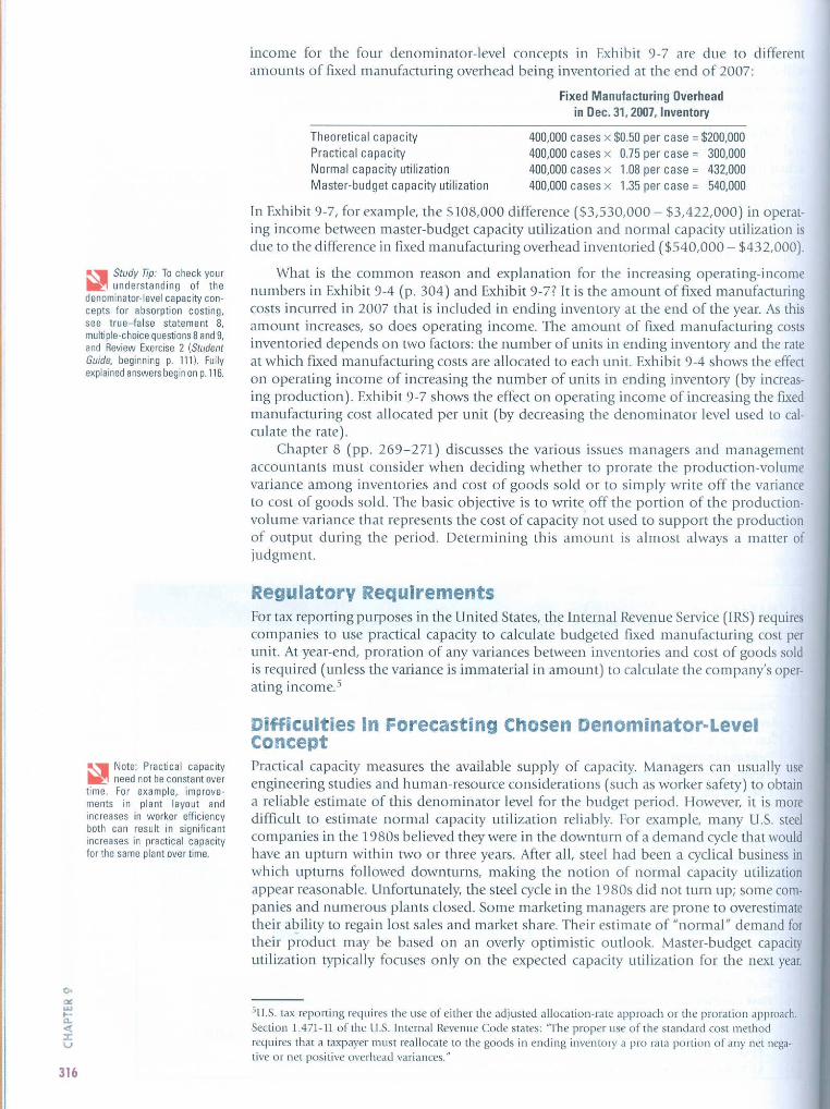
income for the four denominator-level concepts in Exhibit 9-7 are due to differentamounts of ftxed manufacturing overhead being inventoried at the end of 2007:

Fixed Manufacturing Overheadin Dec. 31,2oo7,Invento'1

Theoretical capacityPractical capacityNormal capacity utilizationMaster-budget capacity utilization

400,000cases x $0.50per case = $200,000400,000cases x 0.75per case = 300,000400,000cases x 1.08per case = 432,000400,000cases x 1.35per case = 540,000

c-o<w...0-

•••ru

316

~,. Study Tip: To check yourlIi!lunderstanding of thedenominator-level capacity con-cepts for absorption costing,see true-false statement 8,multiple-choicequestions8and9,and Review Exercise 2 (StudentGuide, beginning p. 111). Fullyexplained answers begin on p. 116.

~ .•• Note: Practical capacityIIi!lneednotbeconstantovertime, For example, improve-ments in plant layout andincreases in worker efficiencyboth can result in significantincreases in practical capacityfor the same plant over time.

In Exhibit 9-7, for example, the $108,000 difference ($3,530,000 - $3,422,000) in operat-ing income between master-budget capacity utilization and normal capacity utilization isdue to the difference in ftxed manufacturing overhead inventoried ($540,000 - $432,000).

\Vhat is the common reason and explanation for the increasing operating-incomenumbers in Exhibit 9-4 (p. 304) and Exhibit 9-77 It is the amount of fIxed manufacturingcosts incurred in 2007 that is included in ending inventory at the end of the year. As thisamount increases, so does operating income. The amount of fixed manufacturing costsinventoried depends on t\\lO factors: the number of units in ending inventory and the rateat which ftxed manufacturing costs are allocated to each unit. Exhibit 9-4 shows the effecton operating income of increasing the number of units in ending inventory (by increas-ing production). Exhibit 9-7 shows the effect on operating income of increasing the fIxedmanufacturing cost allocated per unit (by decreasing the denominator level used to cal·culate the rate).

Chapter 8 (pp. 269-271) discusses the various issues managers and managementaccountants must consider when deciding whether to prorate the production-volumevariance among inventories and cost of goods sold or to simply vvrite off the varianceto cost of goods sold. The basic objective is to write off the portion of the produClion-volume variance that represents the cost of capacity not used to support the productionof output during the period. Determining this amount is almost always a matter ofjudgment.

Regulatory RequirementsFor tax reporting purposes in the United States, the Internal Revenue Service (IRS) requirescompanies to use practical capacity to calculate budgeted fIxed manufacturing cost perunit. At year-end, proration of any variances bet\veen inventories and cost of goods soldis required (unless the variance is immaterial in amount) to calculate the company's oper-ating income.s

Difficulties in Forecasting Chosen Denominator-LevelConceptPractical capacity measures the available supply of capacity. Managers can usually useengineering studies and human-resource considerations (such as worker safety) to obtaina reliable estimate of this denominator level for the budget period. However, it is moredimcult to estimate normal capacity utilization reliably. For example, many U.S. steelcompanies in the 1980s believed they were in the downturn of a demand cycle that wouldhave an upturn within two or three years. After all, steel had been a cyclical business inwhich upturns followed downturns, making the notion of normal capacity utilizationappear reasonable. Unfortunately, the steel cycle in the 1980s did not turn up; some com-panies and numerous plants closed. Some marketing managers are prone to overestimatetheir ability to regain lost sales and market share. Their estimate of "normal" demand fortheir product may be based on an overly optimistic outlook. Master-budget capacityutilization typically focuses only on the expected capacity utilization for the next year.

5U.S. tax reporting requires the use of either the adjusted allocation-rate approach or the proration approach.Section 1.471-11 of the U.S. Internal Revenue Code states: "The proper use of the standard cost methodrequires that a taxpayer must reallocate to the goods in ending inventory a pro r3ta portion of any net nega-tive or net positive overhead variances."

Therefore,master-budget capacity utilization can be more reliably estimated than normalcapacity utilization.

Capacity Costs and Denominator-level Issues\/o,,'e110\".' present more factors that affect the planning and control of capacity costs.

1. Costing systems, such as normal costing or standard costing, do not recognizeuncertainty the way managers recognize it. Managers use a single amount ratherthan a range of possible amounts as the denominator level when calculating bud-geted fixed manufacturing cost per unit in absorption costing. Yet, managers faceuncertainty about demand: they even face uncertainty about their capability to sup-ply. Bushells' plant has an estimated practical capacity of 7,200,000 cases. The esti-mated master-budget capacity utilization for 2007 is 4,000,000 cases. These esti-mates are uncertain. Managers recognize uncertainty in their capacity-planningdecisions. Bushells built its current plant with a 7,200,000-case practical capacity inpart to provide the capability to meet possible demand surges. Even if thesedemand surges do not occur in a given period, it would be wrong to conclude allcapacity not used in a given period is wasted resources. The gains from meeting sud-den demand surges may well require having unused capacity in some periods.

2. The fixed manufacturing cost rate is based on a numerator-budgeted fixed manu-facturing costs-and a denominator-some measure of capacity or capacity utiliza-tion. OUf discussion so far has emphasized issues concerning the choice of thedenominator. Challenging issues also arise in measuring the numerator. For exam-ple, deregulation of the U.S. electric utility industry has resulted in many electricutilities becoming unprofitable. This situation has led to write-downs in the valuesof the utilities' plants and equipment. The write-downs reduce the numeratorbecause there is less depreciation expense included in the calculation of fixed capac-ity cost per kilowatt-hour of electricity produced. The difficulty managers face inthis situation is that the amount of write-dO\vns is not clear-cut but rather a matterof judgment.

3. Capacity costs arise in nonmanufacturing parts of the value chain, as \vell as ,·vith themanufacturing function emphasized in this chapter. Bushells may acquire a fleet ofvehicles capable of distributing the practical capacity of its iced-tea plant. Whenaaual production is belm'\' practical capacity, there ,viii be unused-capacity costissues with the distribution function, as well as with the manufacturing function.

As you saw in Chapter 8, capacity cost issues are prominent in many service-sector companies, such as airlines, hospitals, and railroads, even though these com-panies carry no inventory and so have no inventory costing issues. For example, incalculating the fixed overhead cost per patient-day in its obstetrics and gynecologydepartment, a hospital must decide what denominator level to use: practical capac.ity, normal capacity utilization, or master-budget capacity utilization. Its decisionmay have implications for capacity management, as well as pricing and performanceevaluation.

4. For simplicity and to focus on the main ideas about choosing a denominator tocalculate a budgeted fixed manufacturing cost rate, our Bushells example assumedthat all fixed manufacturing costs had a single cost driver: cases of iced tea pro-duced. As you saw in Chapter 5, activity-based costing systems have multiple over-head cost pools at the output-unit, batch, product-sustaining, and facility-sustaining levels, each with its o'\'n cost driver. In calculating activity cost rates(for fixed costs of setups and material handling, say), management must choosea capacity level for the quantity of the cost driver (setup-hours or loads moved).Should it use practical capacity, normal capacity utilization, or master-budgetcapacity utilization' For all the reasons described in this chapter (such as pricingand capacity management), most proponents of activity-based costing argue thatpractical capacity should be used as the denominator level to calculate activitycost rates.

317

PROBLEM FOR SELF-STUDY

DECISION POINTS

The following question-and-answer format summarizes the chapter's learning objectives. Each decisionpresents a key question related to a learning objective. The guidelines are the answer to that question.

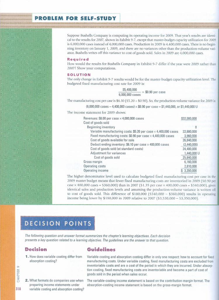
The higher denominator level used to calculate budgeted fixed manufacturing cost per case in the2009 master budget means that fewer fixed manufacturing costs are inventoried in 2009 ($0.90 peTcase x 400,000 cases = 5360,000) than in 2007 ($].35 per case x 400,000 cases = $540,000), givenidentical sales and production levels and assuming the production-volume variance is written offto cost of goods sold. This difference of $180,000 ($540,000 - $360,000) results in operatingincome being lower by $180,000 in 2009 relative to 2007 ($3,530,000 - $3,350,000).

$32,000,000

o22,880,0003,960,000

26,840,00012,440,000124,400,0001,440,000 U

25,840,0006,160,0002,810,000

$ 3,350,000

Variable costing and absorption costing differ in only one respect how to account for fixedmanufacturing costs. Under variable costing, fixed manufacturing costs are excluded frominventoriable costs and are a cost of the period in which they are incurred. Under absorp-tion costing, fixed manufacturing costs are inventoriable and become a part of cost ofgoods sold in the period when sales occur.

The variable-costing income statement is based on the contribution-margin format. Theabsorption-costing income statement is based on the gross-margin format.

Guidelines

Revenues: $8.00 per case x 4,000,000 casesCost of goods sold

Beginning inventoryVariable manufacturing costs: $5.20 per case x 4,400,000 casesFixed manufacturing costs: SO.90per case x 4,400,000 casesCost of goods available for saleDeduct ending inventory: $6.10 per case x 400,000 casesCost of goods sold {at standard costslAdjustment for variances

Cost of goods soldGross marginOperating costsOperating income

SOLUTIONThe only change in Exhibit 9-7 results would be for the master-budget capacity utilization level. Thebudgeted fixed manufacturing cost rate for 2009 is:

$5,400,000 $090= . per case6,000,000 cases

The manufacturing cost per case is $6.10 (55.20 + $0.90). So, the production-volume variance for 2009 is:

16,000,000cases ~ 4,400,000 cases I x $0.90 per case = $1,440,000, or $1,440,000 U

The income statement for 2009 shows:

Suppose Bushells Company is computing its operating income for 2009. That year's results are identi-cal to the results for 2007, shown in Exhibit 9-7, except that master-budget capacity utilization for 2009is 6,OOO,QOO cases instead of 4,000,000 cases. Production in 2009 is 4,400,000 cases. There is no begin-ning inventory on January L 2009, and there are no variances other than the production-volume vari-ance. Bushells writes off this variance to cost of goods sold. Sales in 2009 are 4,000,000 cases.

RequiredIlow would the results for Bushells Company in Exhibit 9·7 differ if the year v·.:ere2009 rather than20D?? Show your computations.

1. How does variable costing differ fromabsorption costing?

2. What formats do companies use whenpreparing income statements undervariable costing and absorption costing?

Decision

3. How do the level of sales and the levelof production affect operating incomeunder variable costing and absorptioncosting?

4. Why might managers build upfinished goods inventory if they useabsorption costing?

5. How does throughput costing differfrom variable costing andabsorption costing?

6. What are the various capacity levelsa company can use to compute thebudgeted fixed manufacturingcost rate?

7. What are the major factors managersconsider in choosing the capacitylevel to compute the budgeted fixedmanufacturing cost rate?

8. Should a company with high fixedcosts and unused capacity raiseselling prices to try to fully recoupits costs?

9. How does the capacity level chosento compute the budgeted fixedoverhead cost rate affect theproduction-volume variance?

Under variable costing, operating income is driven by the unit level of sales. Underabsorption costing, operating income is driven by the unit level of production, the unit levelof sales, and the denominator level.

When absorption costing is used, managers can increase current operating income byproducing more units for inventory. Producing for inventory absorbs more fixedmanufacturing costs into inventory and reduces costs expensed in the period. Critics ofabsorption costing label this manipulation of income as the major negative consequenceof treating fixed manufacturing costs as inventoriable costs.

Throughput costing treats all costs except direct materials as costs of the period in whichthey are incurred. Throughput costing results in a lower amount of manufacturing costsbeing inventoried than either variable or absorption costing.

Capacity levels can be measured in terms of capacity supplied-theoretical capacityor practical capacity. Capacity can also be measured in terms of output demanded-normalcapacity utilization or master-budget capacity utilization.

The major factors managers consider in choosing the capacity level to compute thebudgeted fixed manufacturing cost rate are (a) effect on product costing and capacitymanagement, {bl effect on pricing decisions, lc} effect on performance evaluation,Idl effect on financial statements. lei regulatory requirements, and If I difficulties in forecast-ing chosen capacity-level concepts.

No, companies with high fixed costs and unused capacity may encounter ongoing andincreasingly greater reductions in demand jf they continue to raise selling prices to try tofully recoup variable and fixed costs from a declining sales base. This phenomenon iscalled the downward demand spiral.

When the chosen capacity level exceeds the actual production level, there will be anunfavorable production-volume variance; when the chosen capacity level is less than theactual production level, there will be a favorable production-volume variance.

APPENDIX: BREAKEVEN POINTS IN VARIABLECOSTING AND ABSORPTION COSTING

Breakevenoccurs when the target operating income is $0. In our Stassen illustration for 2007 (seeExhibit 9-2. p. 299):

G= 1$12.000+S10,800)+$0 $22,800$100 -($20 + $19) $61

= 374 units (rounded up to the nearest unit)

Chapter 3 introduced cost-volume-profit analysis. If variable costing is used, the breakeven point[that's where operating income is $0) is computed in the usual manner. There is only onebreakeven point in this case, and it depends on (1) fixed (manufacturing and operating) costsand (2) contribution margin per unit.

The formula for computing breakeven point under variable costing is a special case of themore-general target operating income formula from Chapter 3 (p. 66):

Let Q = Number of units sold to earn the target operating income

Then Q = Total fixed costs + Target operating incomeContribution margin per unit

Proofof break even point:

Revenues, $100 x 374 unitsVariable costs, $39 x 374 unitsContribution margin, $61 x 374 unitsFixed costsOperating income

$37,40014.58622.81422.800

S14

,<•,;;"'<"o!:-5''"o,Q..

"o"a~.-<••,o

'"•~'

Operatingincome is not $0 because the breakeven number of units is rounded up to 374 from 373.77. 319

Operating income is not $0 because the breakeven number of units is rounded up to 2S4 from 283.70.

[Fixed manufacturing x (Brea~eve~ sales _ Units )]

cost rate In units produced

16,15517,145

12,19016,210

16,1965 14

17,127$ 18

$28,400

$33,300

5,39610,800

6,32710,800

$ 9,9402,250 U

$11,6554,500 U

Revenues, $100 x 284 unitsCost of goods sold

Cost of goods sold at standard cost, $35 x 284 unitsProduction-volume variance, $15 x (800 - 650) units

Gross marginOperating costs

Variable operating costs, $19 x 284 unitsFixed operating costs

Operating income

Revenues, $100 x 333 unitsCost of goods sold

Cost of goods sold at standard cost, S35 x 333 unitsProduction-volume variance, $15 x (800 - 500) units

Gross marginOperating costs

Variable operating costs, $19 x 333 unitsFixed operating costs

Operating income

Proof of breakeven point:

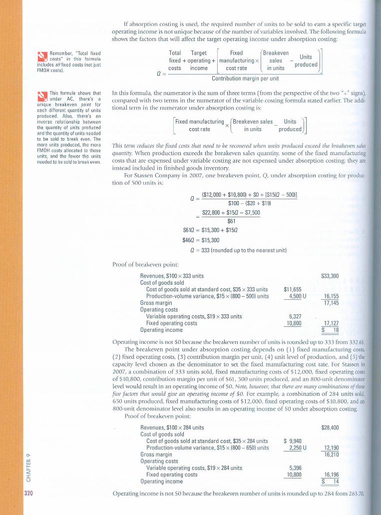
If absorption costing is used, the required number of units to be sold to earn a specific largetoperating income is not unique because of the number of variables involved. The following formulashows the factors that will affect the target operating income under absorption costing:

This tenn reduces the fixed costs that need to be recovered when units produced exceed the breakeven salesquantity. \-"hen production exceeds the breakeven sales quantity, some of the fixed manufacturingcosts that are expensed under variable costing are not expensed under absorption costing; they areinstead included in finished goods inventOI)'.

For Stassen Company in 2007, one breakeven point, Q, under absorption costing for produc-tion of 500 units is:

In this formula, the numerator is the sum of three terms (from the perspective of the two "+" signs),compared with two terms in the numerator of the variable-costing formula stated earlier. The addi·tional term in the numerator under absorption costing is:

0= 1$12,000 + $10,800) + $0 + [515(0 - 5001]$100 - ($20 + $191

522,800 + $150 - $7,500$61

S610 = $15,300 + $150

$460 = $15,300

o = 333 (rounded up to the nearest unitl

~~:~ + o;:;;~~g + [man~~:~~ur;ng x [Br:::::en - U~its dJ]costs income cost rate in units pro uce

O=~~~~~~~~~~~~~~--------~Contribution margin per unit

Operating income is not $0 because the breakeven number of units is rounded up to 333 from 332.61.The breakeven point under absorption costing depends on (1) fixed manufacturing costs,

(2) fixed operating costs, (3) contribution margin per unit, (4) unit level of production, and (5) thecapacity level chosen as the denominator to set the fixed manufacturing cost rate. For Stassen in2007, a combination of 333 unils sold, fixed manufacturing costs of 5 12,000, fixed operating costsof $lO,SOO, contribution margin per unit of $61, 500 units produced, and an SOO-unit denominatorlevel would result in an operating income of $0. Note, however, that there are many combinations ofllwsefive factors Ihal would give an operating il1come of $0. For example, a combination of 2S4 units sold,650 units produced, fixed manufaauring costs of $12,000, fixed operating costs of $lO,SOO, and anSOO-unit denominator level also results in an operating income 6f $0 under absorption costing.

Proof of break even point:

~~ Remember, "Total fixedM!l costs" in this formulaincludes aI/fixed costs (not justFMOH costs).

~, This formula shows thatIII!l under AC, there's aunique breakeven point foreach diflerent quantity of unitsproduced. Also, there's aninverse relationship betweenthe quantity of units producedand the quantity of units neededto be sold to break even. Themore units produced, the moreFMQH costs allocated to thoseunits, and the fewer the unitsneeded to be sold to break even.

320

Suppose actual production in 2007 were equal to the denominator level, 800 units, and therewereno units sold and no fixed operating costs. AlIlhe units produced would be placed in inven-wry, so all the ftxed manufacturing costs would be included in inventory. There would be noproduction-volume variance. Under these conditions, the company could break even with no saleswhatsoever! In contrast, under variable costing, the operating loss vvould be equal to the fixed man~ufacturingcosts of $12,000.

TERMS TO LEARNThischapter and the Glossary at the end of the book contain definitions of:

absorptioncosting (p.1961 normal capacity utilization Ip. 3101directcosting(p.19BI practical capacity Ip. 3101downwarddemandspirallp. 3111 super-variable costing (p. 3051master-budgetcapacity utilization (p. 3101 theoretical capacity (p. 3091

throughput costing (p. 3051variable costing (p. 1961

PH Grad,Assist

Prentice Hall Grade Assist (PHGAIYour professor may ask you to complete selected exercises and problems in Prentice HallGradeAssist IPHGA).PHGAis an online tool that can help you master the chapter's topics.It provides you with multiple variations of exercises and problems designated by the PHGAicon. You can rework these exercises and problems-each time with new data-as manytimes as you need. You also receive immediate feedback and grading.

ASSIGNMENT MATERIAL

Questions

9·1 Differences in operating income between variable costing and absorption costing are duesolely to accounting for fixed costs. Do you agree? Explain.

9·2 Why is the term direct costing a misnomer?9-3 Do companies in either the service sector or the merchandising sector make choices about

absorption costing versus variable costing?9-4 Explain the main conceptual issue under variable costing and absorption costing regarding

the timing for the release of fixed manufacturing overhead as expense.9·5 "Companies that make no variable-cost/fixed-cost distinctions must use absorption costing,

and those that do make variable-cost/fixed-cost distinctions must use variable costing." Doyou agree? Explain.

9·6 The main trouble with variable costing is that it ignores the increasing importance of fixedcosts in manufacturing companies. Do you agree' Why?

9·7 Givean example of how, under absorption costing, operating income could fall even thoughthe unit sales level rises.

9·8 What are the factors that affectthe breakeven point under lal variable costing and (bl absorp-tion costing?

9-9 Critics of absorption costing have increasingly emphasized its potential for leading to unde·sirable incentives for managers. Give an example.

9-10 What are two ways of reducing the negative aspects associated with using absorption cost-ing to evaluate the performance of a plant manager?

9·11 What denominator-level capacity concepts emphasize the output a plant can supply' Whatdenominator-level capacity concepts emphasize the output customers demand for productsproduced by a plant?

9-12 Describe the downward demand spiral and its implications for pricing decisions.9-13 Will the financial statements of a company always differ when different choices atthe start of

the accounting period are made regarding the denominator·level capacity concept?9-14 What is the IRS's requirement for tax reporting regarding the choice of a denominator-level

capacity concept?9·15 "The difference between practical capacity and master·budget capacity utilization is the best

measure of management's ability to balance the costs of having too much capacity and hav-ing too little capacity." Do you agree? Explain. 321

Exercises

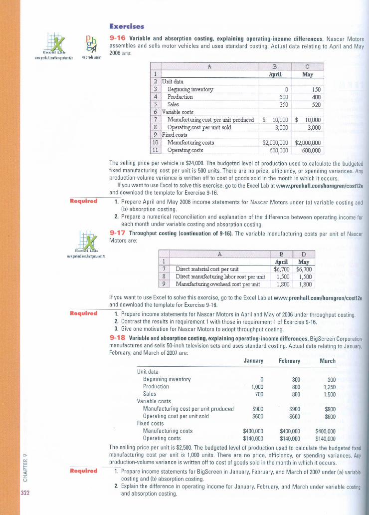
9~16Variable and absorption costing, eXplaining operating· income differences. Nascar Motorsassembles and sells motor vehicles and uses standard costing. Actual data relating to April and May2006 are:

A B C1 ril Ma2 Unit data3 Beginning invento", 0 1504 Production 500 4005 Sales 350 5206 Variable costs7 Manufacturing cost per unit produced $ 10,000 $ 10,0008 Operating cost per unit sold 3,000 3,0009 Fri:edcosts10 Manufacturing costs $2,000,000 $2,000,00011 Operating costs 600,000 600,000

The selling price per vehicle is $24,000. The budgeted level of production used to calculate the budgetedfixed manufacturing cost per unit is 500 units. There are no price, efficiency, or spending variances. Anyproduction-volume variance is written off to cost of goods sold in the month in which it occurs.

If you wantto use Excel to solve this exercise, go to the Excel Lab at www.prenhall.com/horngren/cDst12e__ ._anddownload the template for Exercise 9-16.

R ••• ulr.d 1. Prepare April and May 2006 income statements for Nascar Motors under (a) variable costing andIb) absorption costing.

2. Prepare a numerical reconciliation and explanation of the difference between operating income foreach month under variable casting and absorption casting.

9-17 Throughput costing (continuation of 9-16). The variable manufacturing costs per unit of NascarMotors are:

A B D1 ril Ma7 Direct material cost per unit $6,700 $6,7008 Direct manufacturing labor cost per unit 1,500 1,5009 Manufacturing overhead cost per unit 1,800 1,800

.equl.e"

If you want to use Excel to solve this exercise, go to the Excel Lab at www.prenhall.com/horngren/cost12eand download the template for Exercise 9-16.--------

1. Prepare income statements for Nascar Motors in April and May of 2006 under throughput costing.2. Contrast the results in requirement 1 with those in requirement 1 of Exercise 9-16.3. Give one motivation for Nascar Motors to adopt throughput costing.

9-18 Variable and absorption costing, explaining operating-income differences. BigScreen Corporationmanufactures and sells 50-inch television sets and uses standard costing. Actual data relating to January,February, and March of 2007 are:

January February March

$900$600

3001,2501,500

300800800

ssooSGOO

$900$600

o1,000

700

•••• ulr.d

Unit dataBeginning inventoryProductionSales

Variable costsManufacturing cost per unit producedOperating cost per unit sold

Fixed costsManufacturing costs $400,000 $400,000 $400,000Operating costs $140,000 $140,000 $140,000

The selling price per unit is $2,500. The budgeted level of production used to calculate the budgeted fixedmanufacturing cost per unit is 1,000 units. There are no price, efficiency, or spending variances. Anyproduction-volume variance is written off to cast of goods sold in the month in which it occurs.-------

1. Prepare income statements for BigScreen in January, February, and March of 2007 under (a) variablecosting and (b) absorption costing.

2. Explain the difference in operating income for January, February, and March under variable costingand absorption costing.

'"'"w•..•••«:I:v

322

R•••ulr.d

January February March

Direct material cost per unit S500 $500 $500Direct manufacturing labor cost per unit 100 100 100Manufacturing overhead cost per unit 300 300 300

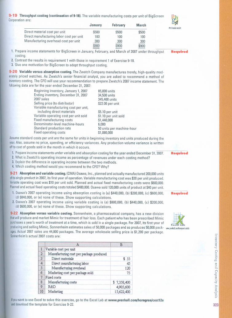
$900 $900 $9001. Prepare income statements for BigScreen in January, February, and March of 2007 under throughput

costing.2. Contrastthe results in requirement 1 with those in requirement 1 of Exercise 9-18.3. Give one motivation for BigScreen to adopt throughput costing.

9-19 Throughput costing (continuation 019-18). The variable manufacturing costs per unit of BigScreen I?hCorporation are: 5J1

85,000 units34.500 units345,400 units$22.00 per unit

9-20 Variable versus absorption costing. The Zwatch Company manufactures trendy, high-quality mod-erately priced watches. As Zwatch's senior financial analyst, you are asked to recommend a method ofinventory costing. The CFO will use your recommendation to prepare Zwatch's 2007 income statement. Thefollowingdata are for the year ended December 31,2007:

Beginning inventory, January 1, 2007Ending inventory, December 31, 20072007 salesSelling price Ita distributorlVariable manufacturing cost per unit,

including direct materials $5.10 per unitVariable operating cost per unit sold $1.10 per unit soldFixed manufacturing costs $1,440.000Denominator-level machine· hours 6,000Standard production rate 50 units per machine-hourFixed operating costs $1,080,000

Assumestandard costs per unit are the same for units in beginning inventory and units produced during theyear.Also, assume no price, spending, or efficiency variances. Any production-volume variance is writtenoffto cost of goods sold in the month in which it occurs .

1. Prepare income statements under variable and absorption costing for the year ended December 31,2007.2. What is Zwatch's operating income as percentage of revenues under each costing method?3, Explain the difference in operating income between the two methods.4. Which costing method would you recommend to the CFD' Why?

9·21 Ahsorption and variable costing. (CMA) Dsawa, Inc., planned and actually manufactured 200,000 unitsofitssingle product in 2007, its first year of operation. Variable manufacturing cost was $20 per unit produced.Variableoperating cost was $10 per unit sold. Planned and actual fixed manufacturing costs were $600,000.Plannedand actual fixed operating costs totaled S400,000. Dsawa sold 120,000 units of product at $40 per unit.

I. Osawa's 2007 operating income using absorption costing is lal $440,000. (b) $200,000. (c) $600,000 .Idl S840.000, or lei none of these. Show supporting calculations.

1. Osawa·s 2007 operating income using variable costing is la} $800,000, (bl $440.000, (cl $200,000,ldl $600,000, or lei none of these. Show supporting calculations.

• equlred

•••• ul •• d

323

$ 5545

12075

$ 7,358,4004,905,600

15,622,400

A1 Variable cost per IlIlit2 ManufllCturing cost per pllCkogeplOdm:ed3 Direct materials4 Direct manufacturing labor5 ManufllCturing overhead6 Marketing cost per pllCkogesold7 Fixedcosts8 ManufllCturing costs9 R&D10 Marketing

9·22 Absorption versus variable costing. Sannenheim, a pharmaceutical company, has a new divisionthat will produce and market Mimic for treatment of hair lass. Each patient who has been prescribed Mimicpurchasesa year's worth of treatment at a time, which is sold in a single package. For 2007, its first year ofproducingand selling Mimic, Sonnenheim estimates sales of 50,000 packages and so produces 50,000 pack-ages.Actual 2007 sales are 44,800 packages. The average wholesale selling price is $1,200 per package.Sonnenheim'sactual 2007 costs are:

If you want to use Excel to solve this exercise, go to the Excel Lab at www.prenhall.com/horngren/cost12eanddownload the template for Exercise 9-22.