exergy methods for the generic analysis and optimization ... · exergy methods for the generic...

Exergy Methods for the Generic Analysis and Optimization of Hypersonic Vehicle Concepts

Kyle Charles Markell

Thesis submitted to the Faculty of the

Virginia Polytechnic Institute and State University

in partial fulfillments of the requirement for the degree of

Master of Science

In

Mechanical Engineering

Dr. Michael von Spakovsky, Chair

Dr. Walter O’Brien

Dr. Michael Ellis

Dr. David Moorhouse

February 7, 2005

Blacksburg, Virginia

Keywords: hypersonics, scramjet, exergy, optimization

Copyright 2005, Kyle Charles Markell

2

Exergy Methods for the Generic Analysis and Optimization of Hypersonic Vehicle Concepts.

by Kyle Charles Markell

Abstract

This thesis work presents detailed results of the application of exergy-based methods to

highly dynamic, integrated aerospace systems such as hypersonic vehicle concepts. In particular,

an exergy-based methodology is compared to a more traditional based measure by applying both

to the synthesis/design and operational optimization of a hypersonic vehicle configuration

comprised of an airframe sub-system and a propulsion sub-system consisting of inlet, combustor,

and nozzle components. A number of key design and operational decision variables are

identified as those which govern the hypersonic vehicle flow physics and thermodynamics and

detailed one-dimensional models of each component and sub-system are developed. Rates of

exergy loss as well as exergy destruction resulting from irreversible loss mechanisms are

determined in each of the hypersonic vehicle sub-systems and their respective components.

Multiple optimizations are performed for both the propulsion sub-system only and for the

entire hypersonic vehicle system for single mission segments and for a partial, three-segment

mission. Three different objective functions are utilized in these optimizations with the specific

goal of comparing exergy methods to a standard vehicle performance measure, namely, the

vehicle overall efficiency. Results of these optimizations show that the exergy method presented

here performs well when compared to the standard performance measure and, in a number of

cases, leads to more optimal syntheses/designs in terms of the fuel mass flow rate required for a

given task (e.g., for a fixed-thrust requirement or a given mission).

In addition to the various vehicle design optimizations, operational optimizations are

conducted to examine the advantage if any of energy exchange to maintain shock-on-lip for both

design and off-design conditions. Parametric studies of the hypersonic vehicle sub-systems and

components are also conducted and provide further insights into the impacts that the design and

operational decision variables and flow properties have on the rates of exergy destruction.

iii

Acknowledgements

This thesis is the product of a great deal of hard work and dedication by many persons. I

would first like to thank my advisor Dr. Michael von Spakovsky for giving me the opportunity to

perform this research, for his faith in my abilities, and for his understanding of the decisions that

were made regarding this thesis. Secondly, I would like to thank my partner in crime for the past

year and a half, Keith Brewer. Keith’s assistance and collaboration on model development and

results generation was invaluable and genuinely appreciated.

Many thanks to Dr. Walter O’Brien, Dr. Michael Ellis, and Dr. David Moorhouse for

serving on my committee, for any input they may have provided throughout the duration of this

work, and for taking time to make draft corrections.

Special thanks to Dr. David Riggins at the University of Missouri-Rolla for his expertise

in hypersonic propulsion and providing many valuable modeling suggestions. Dr. Riggins

prompt responses to the plethora of emails and his willingness to help were greatly appreciated.

This work was conducted under the sponsorship of the U.S. Air Force Office of Scientific

Research. I would like to thank Dr. David Moorhouse, Dr. Jose Camberos, and others at the Air

Force Research Laboratory (AFRL) for their help and guidance on this project and for ultimately

giving me experience through the summer research program at AFRL.

The MooLENI optimization software was provided by the Laboratory of Industrial

Energy Systems (LENI) at Ecole Polytechnique Federale de Lausanne (EPFL) and for that I am

grateful.

I would briefly like to show my appreciation for all my friends from home and to new

friends made in Blacksburg. Even when times were tough, you all manage to keep things

enjoyable and interesting (albeit sometimes too interesting!!). Many thanks to my girlfriend

Lauren for her understanding and generosity and for keeping me focused on my work (and for

those amazing colored drawings!!).

Finally, I would thank my parents for encouraging my decision to further my education,

for their constant support, and of course let’s not forget their financial support at times.

Kyle Charles Markell

iv

Table of Contents

ABSTRACT ii

AKNOWLEDGEMENTS iii

TABLE OF CONTENTS iv

LIST OF FIGURES vii

LIST OF TABLES xi

NOMENCLATURE xiii

CHAPTER 1 INTRODUCTION 1

1.1 General Background/History of Hypersonic Vehicles 1

1.1.1 Hypersonic Flight- What is it? and Why is it Important 2

1.1.2 Advancements and Milestones in Hypersonic Flight 4

1.2 Hypersonic Vehicle Design Challenges 8

1.2.1 Hypersonic Vehicle versus Conventional Aircraft 8

1.2.2 Ramjet versus Scramjet Engines 9

1.2.3 The Need for a Unified Approach to Hypersonic Vehicle Sythesis\Design 10

1.3 Thesis Objectives 11

CHAPTER 2 LITERATURE REVIEW 14

2.1 Synthesis/Design Analysis and Optimization of High Performance Aircraft 14

2.1.1 Subsonic/Supersonic Advanced Fighter Concepts 14

2.1.2 Hypersonic Vehicle Concepts 17

2.2 Exergy-Based Methods in the Design/Analysis of Hypersonic Vehicles 25

2.2.1 Work Potential/Thrust Potential Methods 26

2.2.2 Exergy Methods for System-Level Multidisciplinary Analysis 33

2.2.3 Additional Exergy/Available Energy Research in Advanced Aircraft Analysis 36

CHAPTER 3 HYPERSONIC AIRBREATHING PROPULSION TECHNICAL BACKGROUND 38

3.1 Fundamental Definitions and Relations 38

3.2 Shock/Expansion Overview 45

v

3.2.1 Oblique Shock Theory 45

3.2.2 Gradual Compressions 50

3.2.3 Prandtl Meyer Flow 52

3.3 Hypersonic Vehicle and Component Description/Investigation 54

3.3.1 Inlet Compression and Isolator Components 55

3.3.2 Combustion Component 63

3.3.3 Expansion Component 67

CHAPTER 4 COMPREHENSIVE SUB-SYSTEM AND COMPONENT MODELS 69

4.1 Propulsion Sub-system Description 69

4.1.1 Inlet Component Description and Modeling 69

4.1.2 Combustor Component Description and Modeling 80

4.1.3 Nozzle Component Description and Modeling 94

4.2 Airframe Sub-system Description and Modeling 98

4.2.1 Vehicle Volume and Center of Gravity Estimation 99

4.2.2 Force Accounting and Moment Trim 100

4.2.3 Wing and Elevon Details 104

4.2.4 Mass Fraction and Weight Estimation 107

4.2.5 Airframe Sub-system Constants and Constraints 109

CHAPTER 5 SYNTHESIS/DESIGN OPTIMIZATION PROBLEM DEFINITION AND STRATEGY 111

5.1 Problem Definition 111

5.2 Optimization Technique 113

5.2.1 Evolutionary Algorithms (EAs) 115

5.2.2 MooLENI Evolutionary Algorithm 117

5.2.3 QMOO Test Problem 118

5.3 Design Problem Simulation and Coupling to EA 119

CHAPTER 6 RESULTS AND DISCUSSION 121

6.1 Preliminary Analysis Using Exergy Mehtods 121

6.2 Hypersonic Vehicle Component Parametric Studies 124

6.3 Scramjet Engine Only Optimizations and Study 134

6.4 Single Mission Segment Optimizations and Partial Mission Optimizations 145

vi

CHAPTER 7 CONCLUSION 160

APPENDIX A 163

APPENDIX B 164

APPENDIX C 169

REFERENCES 170

VITA 176

vii

List of Figures

Figure 1-1 Conceptual scramjet powered hypersonic vehicles (Anderson [3]) 5

Figure 1-2 Artist’s rendition of the X-43A hypersonic experimental vehicle in flight 7

Figure 1-3 The actual X-43A hypersonic vehicle during ground testing 7

Figure 2-1 Representation of baseline configuration defined by Bowcutt [36]. Configuration shows independent and dependent variables. 18

Figure 2-2 Representation of the optimal (a) Mach 10 cruise scramjet integrated waverider, (b) Mach 10 accelerator scramjet integrated waverider, and (c) Mach 8 cruise scramjet integrated waverider determined by O’Neil and Lewis [41] 23

Figure 2-3 Loss of available gas specific power during F-5E area intercept mission (Roth and Marvis [15]) 29

Figure 2-4 Thrust potential and losses versus axial distance for engine flowfield (Riggins, McClinton, and Vitt [10]) 31

Figure 3-1 Forces acting on an aerospace vehicle in flight 39

Figure 3-2 Standard day geometric altitude versus flight Mach number trajectories for constant dynamic pressure (Heiser et al. [1]) 41

Figure 3-3 Equilibrium ratio of specific heats of air as a function of static temperature and static pressure (Heiser et al. [1]) 42

Figure 3-4 Equilibrium mole fraction composition for several constituents of air as a function of temperature. Static pressure fixed at 0.01 atm (Heiser et al. [1]) 43

Figure 3-5 Wedge shock 46

Figure 3-6 Corner shock 46

Figure 3-7 Oblique shock diagram 47

Figure 3-8 Shock angle versus deflection angle 49

Figure 3-9 Abrupt compression of flow 51

Figure 3-10 Gradual compression of flow 51

Figure 3-11 Prandtl-Meyer expansion 52

viii

Figure 3-12 Generic propulsion sub-system terminology/components 54

Figure 3-13 External oblique shock wave compression component 56

Figure 3-14 Mixed external and internal compression component 56

Figure 3-15 Mass flow spillage and area definitions 59

Figure 4-1 A physical representation of the inlet compoent(front undersurface of the vehicle). The decision and operational variables that govern the flow characteristics throughout the inlet are displayed along with the flow velocity vector from freestream to inlet exit 70

Figure 4-2 Inlet interface and vehicle surface definitions along with some basic area and height representations. 71

Figure 4-3 Close up view of the cowl oblique shock and inlet throat region 74

Figure 4-4 Conceptual diffuser used to approximate the irreversibility rate due to skin friction 75

Figure 4-5 Isolated solver description used to calculate combustor entrance properties 76

Figure 4-6 Oblique shock tailoring with energy exchange 79

Figure 4-7 Combustor component schematic with station numbers 81

Figure 4-8 Mixing layer differential element 83

Figure 4-9 Axial growth of the mixing and combustion efficiencies for the combustor component 87

Figure 4-10 Isobaric batch reaction of stoichiometric hydrogen and air mixture. Initial conditions are: P = 2 atm, T = 1500 K (Heiser et al. [1]) 93

Figure 4-11 Nozzle component schematic including station numbers and other geometric parameters 96

Figure 4-12 Reference points for vehicle volume calculation 99

Figure 4-13 Five panels used to estimate the center of gravity. Each panel has its own centroid marked by a bullet. The actual vehicle surface is displayed in light, small dashed lines 100

Figure 4-14 Airframe and propulsive forces acting on the hypersonic vehicle 102

Figure 4-15 Plan view of vehicle showing wing and elevon concepts 104

ix

Figure 4-16 Diamond airfoil cross-section used to describe the wing and elevon. A given angle-of-attack and freestream properties produce a pressure distribution as shown. The airfoil thickness and chord length are shown as well 105

Figure 5-1 Mission profile by segment 112

Figure 5-2 Woods function contour plot with x3 = x4 =1 119

Figure 6-1 Optimal combustor length design problem 122

Figure 6-2 Optimal combustor lengths predicted by engine and thermodynamic effectiveness 124

Figure 6-3 Specific exergy destruction versus specific thrust for a range of ramp lengths and forebody angles with the fixed design decision variables values listed in Table 6-2 126

Figure 6-4 Specific exergy destruction versus specific thrust for a range of combustor lengths and nozzle expansion angles with the fixed design decision variable listed in Table 6-2 127

Figure 6-5 Specific exergy destruction versus the specific thrust for a range of nozzle expansion angles and percent cowl lengths with fixed design decision variable values listed in Table 6-2 128

Figure 6-6 The effect of design decision variable cowl% on the nozzle upward suface force and nozzle moment. 129

Figure 6-7 Specific exergy destruction versus the compression efficiency for a range of ramp lengths and forebody angles with the fixed design decision variable values listed in Table 6-2 129

Figure 6-8 Specific exergy destruction versus the kinetic energy efficiency for a range of ramp lengths and forebody angles with the fixed design decision variable values listed in Table 6-3 130

Figure 6-9 Rate of exergy destroyed by combustor loss mechanisms at M5 = 3.2 and over a range of combustor entrance temperatures (T5) and pressures (P5). Molecular weight and specific heat ratio are fixed 131

Figure 6-10 Rate of exergy destroyed by combustor loss mechanisms at M5 = 3.2 and over a range of combustor entrance temperatures (T5) and pressures (P5). Molecular weight and specific heat ratio changes are included in the combustor model 132

x

Figure 6-11 Specific exergy destruction of the propulsion sub-system components over a range of flight Mach numbers. Energy exchange included in the propulsion sub-system 137

Figure 6-12 Specific exergy destruction of propulsion system components over range of flight Mach numbers. No energy exchange in propulsion system 138

Figure 6-13 Rate of exergy destruction of the propulsion sub-system components for each of the optimal flight Mach number scramjet engines 141

Figure 6-14 Exergy destruction due to individual loss mechanisms for each of the optimal flight Mach number scramjet engines 142

Figure 6-15 3D CAD representation of a typical Mach 10 hypersonic cruise vehicle 152

Figure A-1 Optimal inlet component configurations for the scramjet engine (propulsion sub-system) only optimizations 163

Figure B-1 Optimal Mach 8 cruise vehicles for the single segment optimizations using the objective functions ηo and Exdest . Both the vehicle plumes and centers of gravity are shown in the figure 164

Figure B-2 Optimal Mach 8-10 accelerator vehicles for the single segment optimizations using the objective functions ηo and Exdest . Both vehicle plumes and centers of gravity are shown in the figure 165

Figure B-3 Optimal Mach 8-10 accelerator vehicles for the single segment optimizations using the objective functions ηo and Exdest + Exloss. Both vehicle plumes and centers of gravity are shown in the figure 166

Figure B-4 Optimal Mach 10 cruise vehicles for the single segment optimization using the objective functions ηo and Exdest . Both vehicle plumes and centers of gravity are shown in the figure 167

Figure B-5 Optimal Mach 10 cruise vehicles for the single segment optimization using the objective functions ηo and Exdest + Exloss. Both vehicle plumes and centers of gravity are shown in the figure 168

Figure C-1 Optimal partial mission vehicles for objective functions ηo and Exdest + Exloss 169

xi

List of Tables

Table 3-1 Gradual compression example results 51

Table 5-1 Mission specifications 113

Table 5-2 Woods function optimization results 118

Table 5-3 Design decision variables and limits 120

Table 5-4 Operational decision variables and limits 120

Table 6-1 Comparison of optimal combustor models 124

Table 6-2 Design decision variable fixed values and ranges for component audits 125

Table 6-3 Combustor effects due to molecular weight/specific heat ratio changes 134

Table 6-4 Scramjet engine with and without energy exchange 135

Table 6-5 Optimal Mach 10 scramjet configurations 139

Table 6-6 Optimal design decision variables and parameters for optimal scramjet engines 140

Table 6-7 Energy and exergy based optimizations for a scramjet engine with fixed thrust 144

Table 6-8 Partial mission specifications 146

Table 6-9 Design variable values for single segment optimizations 147

Table 6-10 Calculated optimal parameter values for single mission segment optimizations 149

Table 6-11 Mission segment fuel mass fractions 153

Table 6-12 Optimal design decision variable values for the partial mission 155

Table 6-13 Optimal operational decision variable values for the partial mission 155

Table 6-14 Calculated optimal parameter values at each segment of the partial mission 156

Table 6-15 Vehicle optimum fuel mass flow rate comparison 157

xii

Table 6-16 Comparison of initial feasible vehicle and final optimal vehicle using the exergy objective function 158

Table 6-17 Comparison of initial feasible vehicle and final optimal vehicle using the overall efficiency objective function 158

xiii

Nomenclature

A Area, fit parameter F Force, streamthrust

B Fit paramter fst Stoichiometric fuel-to-air ratio

CD Drag coefficient GHz Gigahertz

CL Lift coefficient g Acceleration of gravity

Cp Pressure coefficient H, h Height, enthalpy

Cm Mixing constant H2 Hydrogen

Cf Skin friction coefficient H2O Water

CR Contraction ratio hpr Fuel lower heating value (LHV)

cp Constant pressure specific heat

Isp Specific impulse

cv Constant volume specific heat ICR Internal contraction ratio

c.s. Control surface L Lift, length

D Drag Lm Length for minor mixant to be depleted

Dh Hydraulic diameter M Mach number

E Energy MHD Magnetohydrodynamics

Ex, ex Exergy MB Megabytes

m& Mass flow rate S, s Entropy, planform area

xiv

m Mass T Thrust, static temperature

N2 Nitrogen t Time, thickness

n Load factor U, u Velocity

nm Nautical miles V Velocity

n& Molar flow rate ∀ Volume

O2 Oxygen W, w Weight, work

P Static pressure, power X Length, distance

Pr Prandtl number xcg Axial location of the center of gravity

Q , q Heat ycg Vertical location of the center of gravity

q0 Dynamic pressure y Fuel-to-air axial velocity ratio, mole fraction

R Specific gas constant, range z Elevation

RAM Random Access Memory

Rex Reynolds number

r Recovery factor

xv

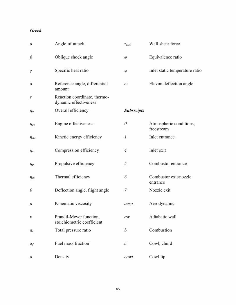
Greek

α Angle-of-attack τwall Wall shear force

β Oblique shock angle φ Equivalence ratio

γ Specific heat ratio ψ Inlet static temperature ratio

δ Reference angle, differential amount

ω Elevon deflection angle

ε Reaction coordinate, thermo-dynamic effectiveness

ηo Overall efficiency Subsrcipts

ηee Engine effectiveness 0 Atmospheric conditions, freestream

ηKE Kinetic energy efficiency 1 Inlet entrance

ηc Compression efficiency 4 Inlet exit

ηp Propulsive efficiency 5 Combustor entrance

ηth Thermal efficiency 6 Combustor exit/nozzle entrance

θ Deflection angle, flight angle 7 Nozzle exit

µ Kinematic viscosity aero Aerodynamic

ν Prandtl-Meyer function, stoichiometric coefficient

aw Adiabatic wall

πc Total pressure ratio b Combustion

πf Fuel mass fraction c Cowl, chord

ρ Density cowl Cowl lip

xvi

comb Combustor opt Optimal

c.v. Control volume p Pressure

des Destruction ramp1 (r1) First inlet ramp

elev Elevon ramp2 (r2) Second inlet ramp

fb Forebody s Surface, shaft

f Friction, fuel surf Surface

fric Friction t Total

g Gas vap Vaporization

ht Heat transfer veh Vehicle

inc. comb. Incomplete combustion w wall

irr Irreversibility

ic Internal compression Superscripts

M Mixing * Reference conditions

mix Mixing, mixture

need Required amount

nozz Nozzle

1

Chapter 1

Introduction

The topic of and research in airbreathing propulsion via ramjet and scramjet engines is far

from novel, dating back many decades1. These engines are attractive as propulsive devices

because of their ability to sustain high speed atmospheric flight. Fluctuations in interest in and

research on ramjet and scramjet engines have occurred over the past half century. However a

rebirth of activity in recent year has occurred because the significant performance improvements

promised by airbreathing propulsion have become attainable through the advancement of the

underlying technologies. Therefore, this introductory chapter is dedicated to the explanation and

importance of hypersonic flight and ramjet and scramjet engines as well as the presentation of

some hypersonic flight milestones. This chapter also presents some of the design challenges

associated with hypersonic vehicles and, finally, the objectives of this thesis are given.

1.1 General Background/History of Hypersonic Vehicles

It is important to understand what is really meant by the term hypersonic and what the

significance of hypersonic flight truly is. A clear depiction of what a hypersonic vehicle may

look like is essential to the comprehension of the material presented in this thesis and, therefore,

a few hypersonic vehicle concepts are presented in this section. Furthermore, it is interesting to

see and serves the purpose of describing the advancements and milestones in hypersonic flight in

order to establish a mental picture progression of the field and possibly some of the lessons

learned.

1 In fact, the notion of using a ramjet engine as a propulsive device dates back to the early 1900’s [1].

2

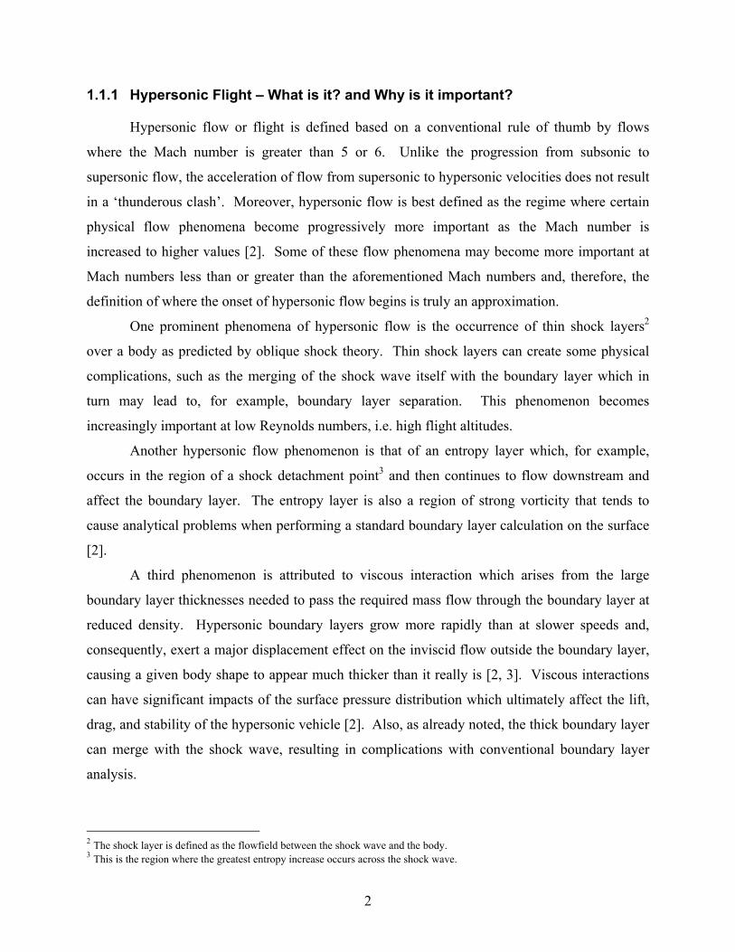
1.1.1 Hypersonic Flight – What is it? and Why is it important?

Hypersonic flow or flight is defined based on a conventional rule of thumb by flows

where the Mach number is greater than 5 or 6. Unlike the progression from subsonic to

supersonic flow, the acceleration of flow from supersonic to hypersonic velocities does not result

in a ‘thunderous clash’. Moreover, hypersonic flow is best defined as the regime where certain

physical flow phenomena become progressively more important as the Mach number is

increased to higher values [2]. Some of these flow phenomena may become more important at

Mach numbers less than or greater than the aforementioned Mach numbers and, therefore, the

definition of where the onset of hypersonic flow begins is truly an approximation.

One prominent phenomena of hypersonic flow is the occurrence of thin shock layers2

over a body as predicted by oblique shock theory. Thin shock layers can create some physical

complications, such as the merging of the shock wave itself with the boundary layer which in

turn may lead to, for example, boundary layer separation. This phenomenon becomes

increasingly important at low Reynolds numbers, i.e. high flight altitudes.

Another hypersonic flow phenomenon is that of an entropy layer which, for example,

occurs in the region of a shock detachment point3 and then continues to flow downstream and

affect the boundary layer. The entropy layer is also a region of strong vorticity that tends to

cause analytical problems when performing a standard boundary layer calculation on the surface

[2].

A third phenomenon is attributed to viscous interaction which arises from the large

boundary layer thicknesses needed to pass the required mass flow through the boundary layer at

reduced density. Hypersonic boundary layers grow more rapidly than at slower speeds and,

consequently, exert a major displacement effect on the inviscid flow outside the boundary layer,

causing a given body shape to appear much thicker than it really is [2, 3]. Viscous interactions

can have significant impacts of the surface pressure distribution which ultimately affect the lift,

drag, and stability of the hypersonic vehicle [2]. Also, as already noted, the thick boundary layer

can merge with the shock wave, resulting in complications with conventional boundary layer

analysis.

2 The shock layer is defined as the flowfield between the shock wave and the body. 3 This is the region where the greatest entropy increase occurs across the shock wave.

3

The most significant aspect of hypersonic flow is the very high temperatures that can

occur within the hypersonic boundary layers and in the nose region of blunt bodies. Extreme

temperatures tend to cause dissociation of the gas molecules and possibly ionization within the

gas and, therefore, the proper inclusion of chemically reacting effects is vital to the calculation of

an accurate shock layer temperature [2, 3]. In some instances, temperatures as high as 10,000 K

or more4 occur in the shock layer or nose region of a hypersonic vehicle, especially during

atmospheric reentry. Like viscous interaction, high temperature chemically reacting flows can

have an influence on lift, drag, and moments on a hypersonic vehicle [2]. The most dominant

aspect of high temperature hypersonic flows is the large convective heat transfer rates to the

surface and possibly rather large radiative heating, both of which have a substantial influence on

material selection.

A final characteristic of hypersonic aerodynamics is low-density flows that occur at

extreme altitudes. Under these conditions, the aerodynamic concepts, equations, and results

based on the assumption of a continuous medium (i.e. continuum) begin to break down and,

consequently, methods from kinetic theory must be used to predict the aerodynamic behavior [2].

Additionally, an altitude can be reached where the conventional ‘no-slip’ condition begins to fail

and the gas temperature at the surface of the vehicle does not equal the surface temperature of

the material.

The development of aviation and aircraft has been continuously driven by the urge to fly

faster and at higher elevations and attain greater flight ranges. To continue this trend, the

development of hypersonic vehicles and the employment of ramjet and scramjet engines

becomes ever more important. These vehicles and engines offer the potential to reduce the cost

and increase the dependability of transporting payloads5 to Earth orbits [1].

For example, consider the case of a rocket where, typically, greater than 60% of the

takeoff weight is oxidizer (oxygen) and less than 5% of the takeoff weight is payload. This large

fraction of oxygen reduces the weight fraction available for empty weight (including structures,

propulsion, controls, etc.) which compromises ruggedness and flexibility [1]. If ramjet or

scramjet engines are substituted for rockets, the oxidizer no longer needs to be carried along (i.e.

these engines are air breathers) and is beneficial because

4 These temperatures are about twice the surface temperature of the sun. 5 In general terms, a payload could be a radar antenna, satellite, weapons for delivery, etc.

4

1. The takeoff weight fraction of the payload can be increased substantially.

2. The weight saved by leaving the oxygen behind could be used to make the vehicle (rocket)

smaller while increasing the empty weight fraction and thereby improving the ruggedness

and flexibility.

3. More fuel can be used to attain a greater range for payload delivery.

4. The reduced vehicle size and weight and the increased payload-to-takeoff weight ratio can

help reduce payload delivery costs significantly.

Additionally, ramjet and scramjet offer the potential for higher sustainable velocities and

ultimately faster delivery of the payload.

A few scramjet powered hypersonic vehicle concepts are depicted in Figure 1-1,

including a strike/reconnaissance vehicle and space access vehicle. The strike/reconnaissance

vehicle could be manned or unmanned and would have the ability to complete a mission much

faster and more efficiently then presently possible. This concept of vehicle may be likened to the

SR-71 Blackbird, which was a fairly high supersonic reconnaissance aircraft (attained flight

speeds of Mach 3) that flew a few thousand successful missions without being shot down. The

space vehicle concept is similar to that proposed by the United States National Aero-Space

Program (NASP) which was a joint program between the Department of Defense and NASA.

The goal of the NASP program was to develop and demonstrate the feasibility of a piloted,

horizontal takeoff and landing aircraft that utilized conventional airfields, accelerated to

hypersonic speeds, achieved orbit in a single stage, delivered useful payloads to space, returned

to Earth with propulsive capability, and had the operability, flexibility, supportability, and

economic potential of airplanes [1]. Another capability of hypersonic vehicles is hypersonic

transport. These are contemporary ideas for hypersonic vehicles to cruise at Mach 7 to 12 and

carry people from New York to Tokyo in less than two hours [2].

1.1.2 Advancements and Milestones in Hypersonic Flight

The notion of using ramjet engines as propulsive devices, as already mentioned, has

been recognized since the early 1900s. However, it wasn’t until 1946 when the first pure ramjet

propulsion of a piloted aircraft took place; two ramjet engines were mounted on the wingtips of a

Lockheed F-80. Then in 1949 the first piloted ramjet engine and airframe integrated aircraft, the

Leduc 010, achieved successful ramjet propulsion and reached a Mach number of 0.84.

5

Figure 1-1. Conceptual scramjet powered hypersonic vehicles (From Anderson Jr., J. D., Fundamentals of Aerodynamics, 3rd Edition, McGraw-Hill, New York, 2001 [3]; reprinted by permission of The McGraw-Hill Companies).

Shortly thereafter, the U.S. Air Force sponsored the Lockheed Aircraft Company X-7 and X-7A

supersonic reusable pilotless flight research program. These vehicles were boosted by a solid

rocket to ramjet takeover velocities and then propelled into sustained flight by ramjets. This

program provided much significant ramjet performance information for Mach numbers up to

approximately 4.3. Also during this timeframe, the use of ramjets for missile propulsion became

6

more attractive because of the ability to achieve greater range for the same propellant weight and

because these systems were relatively simple with low initial costs. [1]

The first object of human origin to achieve hypersonic flight was that of a slender,

needle-like rocket called the WAC Corporal. This rocket was mounted on the top of a V-2

rocket and served as a second stage to the V-2, ultimately detaching, igniting, and attaining a

flight velocity of over 5000 mph. This was, of course, followed by the space age which began in

1961 when Russia’s Flight Major Yuri Gagarin became the first human in history to experience

hypersonic flight. Gagarin’s orbital craft, the Vostok I, was launched into orbit, attained free

flight around the earth and returned safely. Later that year Alan Shepard became the second man

in space by virtue of a suborbital flight over the Atlantic Ocean where he entered the atmosphere

at a speed above Mach 5.

The Hypersonic Research Engine (HRE) program was implemented by NASA in 1964 to

develop scramjet engines. The goal of the HRE program was to test a complete, regeneratively

cooled, flightweight scramjet engine on the X-15A-2 rocket research airplane. The X-15A-2

flew several times, achieving a maximum flight Mach number of 6.72 while having a dummy

ramjet attached to its ventral fin. This program was ended prematurely though because of

damage sustained to the rocket during its record breaking flight. In more recent times (early

1990s), the Russian Central Institute of Aviation Motors designed and launched a subscale, dual

mode, ramjet and scramjet airbreathing engine mounted on the nose of a rocket for captive

testing. This project not only sustained scramjet operation for 15 seconds, it also demonstrated

ramjet to scramjet transition under realistic flight conditions. [1, 2]

The most recent demonstration of hypersonic flight and scramjet engines took place twice

over the past year. Two successful flights of a subscale, unpiloted hypersonic vehicle, named the

X-43A, demonstrated the capability of attaining high Mach number flight using air-breathing

engines. The X-43A is a hypersonic aircraft developed under NASA’s Hyper-X program. This

program aimed to flight validate key propulsion and related technologies for air-breathing

hypersonic aircraft and ultimately sought to expose the promise to increase payload capacities

and reduce costs for future space and air travel. The latest flight brought to an end the eight year,

$200 million plus program that incorporated three test flights. A depiction of the X-43A in flight

in given in Figure 1-2 and the actual vehicle used in the test flights is shown in Figure 1-3.

7

Figure 1-2. Artist’s rendition of the X-43A hypersonic experimental vehicle in flight. Photo taken from

the website http://www.drfc.nasa.gov/Gallery/Photo/X-43A/HTML/index.html.

Figure 1-3. The actual X-43A hypersonic vehicle during ground testing. Photo taken from the website http://www.drfc.nasa.gov/Gallery/Photo/X-43A/HTML/index.html.

The X-43A is approximately 12 ft in length with a span of about 5 ft and is powered by a

hydrogen fueled scramjet engine. For all test flights, the X-43A was mounted on the front of a

booster rocket in which the rocket itself was mounted on a B-52B launch aircraft. The B-52B

carried the rocket and X-43A to a given altitude and then launched the booster rocket. The

booster rocket then took the X-43A to its desired test altitude and speed where at that point the

X-43A separated from the rocket and flew for several minutes. The first test flight took place in

June, 2001 but came to an abrupt end when the rocket and test vehicle had to be destroyed in

mid-flight. The second test flight took place in March, 2004 where the X-43A was deployed at

approximately 95,000 ft and successfully maintained a test flight Mach number of 7 under 10

8

seconds of scramjet engine operation. The final test flight occurred in November, 2004 where

the X-43A separated from the rocket at around 110,000 ft. and cruised at Mach 9.6 (a little less

than 7,000 mph) for 20 seconds of scramjet engine supplied power. The final test flight

experienced approximately one-third hotter temperatures than the Mach 7 flight.

1.2 Hypersonic Vehicle Design Challenges

There are many design challenges associated with achieving hypersonic airbreathing

propulsion because of the large range of flight operating conditions experienced and the highly

integrated nature of the entire vehicle. Therefore, this section compares hypersonic vehicles with

conventional high performance aircraft, describes hypersonic propulsion systems and their

integration into the airframe, and also discusses the need for a common metric in hypersonic

vehicle synthesis/design.

1.2.1 Hypersonic Vehicle versus Conventional Aircraft

Conventional subsonic and supersonic aircraft are designed such that the components for

providing lift, propulsion, and volume (i.e. the wings, engines, and fuselage, respectively) are not

strongly coupled to one another. The components are separate and distinct, i.e. each treated as a

separate aerodynamic body and, when combined to form the entire aircraft, only interact

moderately. Moreover, these components can be designed separately and still provide the

necessary flight performance. The planform area of the wing supplies the lift necessary for flight

and the engines contain rotating machinery to decelerate (compress) and accelerate (expand) the

freestream flow. In addition, subsonic and supersonic aircraft operate over a fairly narrow flight

Mach number range6.

In contrast to conventional aircraft synthesis/design, the aerodynamic surfaces and the

propulsive devices of a hypersonic vehicle are highly integrated. In fact, the entire undersurface

of the vehicle serves as part of the scramjet engine. Compression of the freestream flow takes

6 The statements made in this paragraph are completely consistent for the design of commercial and military transport aircraft but, to some point, are less applicable to advanced fighter aircraft design. Although advanced fighter aircraft have large, distinct wings for production of lift, they typically have portions of their engines integrated within the airframe which consequently results in some coupling of the components. However, advanced fighters are not nearly integrated to the degree of hypersonic vehicle configurations.

9

place on the front undersurface of the vehicle and is accomplished through a series of oblique

shock waves generated as a result of flow deflection. Hydrogen fuel is burned in the supersonic

combustor and is also used to cool vehicle surfaces. The combusted gases are expanded using

the aft undersurface of the vehicle as an expansion nozzle. Most of the vehicle lift is produced

by the high pressures on the compression and expansion surfaces and, therefore, large, distinct

wings are not necessary for the production of lift. In addition, forces and moments change rather

significantly in a nonlinear fashion with angle of attack. These are just a few reasons for the

highly coupled aerodynamic and propulsion sub-systems of a hypersonic vehicle, i.e. changes to

the propulsion sub-system inherently affect the vehicle aerodynamics. Furthermore, hypersonic

vehicles are designed to traverse the atmosphere over rather large flight conditions (e.g., Mach 0

– 15) and, thus, need to be synthesized/designed to operate efficiently over these flight ranges.

Hypersonic vehicles will ultimately incorporate both ramjet and scramjet propulsion in the

vehicle, which adds further complexities to the synthesis/design. Finally, unlike conventional

aircraft, hypersonic vehicles experience the various phenomena described in Section 1.1.1.

Capitalizing on vehicle surfaces for compression and expansion, as explained above, is

essential to the success of the hypersonic vehicle synthesis/design. It was discovered in early

hypersonic tests that making the hypersonic engines axisymmetric and attaching them to the

vehicle using pylons or struts can produce enough external drag on the pylon and cowl to

virtually cancel the internal thrust as well as producing internal flowfields that are difficult to

manage [1].

1.2.2 Ramjet versus Scramjet Engines

Although ramjets can operate at subsonic flight speeds, they are predominately used for

supersonic flight, specifically in the approximate Mach number range of 3 to 6. The freestream

flow is compressed via a diffuser and is usually accomplished in several steps. The supersonic

flow is initially decelerated by one or more oblique shock waves generated by the forebody of

the vehicle or diffuser, further decelerated in a convergent duct, and then transformed into

subsonic flow through a normal shock wave system. The subsonic flow may be further

decelerated by a divergent duct to Mach numbers of about 0.2 to 0.3 where fuel is injected and

burned in the combustor which typically contains a flameholder to stabilize the flame. The

10

burned gases are accelerated/expanded in a convergent-divergent nozzle and are exhausted into

the atmosphere at supersonic speeds to provide the engine thrust.

At flight Mach numbers of about 6 and greater, the conversion of the freestream kinetic

energy to internal energy via the compression system results in rather large combustor entrance

pressures, temperatures, and densities. So pronounced is the effect that it is no longer

advantageous to decelerate the flow to subsonic speeds. Adverse consequences can include

pressures too high for practical burner structural design, excessive performance losses due to the

normal shock system, excessive wall heat transfer rates, and combustion conditions that lose a

large fraction of the available chemical energy to dissociation [1].

To avoid these problems, the flow is only partially compressed and decelerated using a

supersonic combustion ramjet (i.e. scramjet) where the flow entering the combustor is

supersonic. However, in contrast to ramjets, the scramjet engine diffuser takes greater advantage

of the inevitable compression by the vehicle surface and the main compression mechanism is the

oblique shock waves generated from the vehicle forebody and compression ramps. The diffuser

is strictly convergent and, therefore, the flow entering the combustor is supersonic. Emphasis is

placed upon mixing in the combustor because the supersonic flow throughout the combustor

produces short available combustion times. Scramjet combustors will more than likely use

hydrogen as fuel whereas ramjets typically burn some form of hydrocarbon fuel. The burned

gases are then accelerated/expanded using only a divergent nozzle which tends to be the

afterbody surface of the vehicle.

Note that, for both of these engines, it is convenient to use the outside surface of the

vehicle as the boundary of the engine. In addition, both of these engines are capable of

producing large amounts of thrust in their respective flight regimes. Unfortunately, both ramjet

and scramjet engines are incapable of developing static thrust and, therefore, cannot accelerate a

vehicle from a standing start.

1.2.3 The Need for a Unified Approach to Hypersonic Vehicle Synthesis/Design

Conventional aircraft systems and subsystems traditionally have been designed relying

heavily on rules-of-thumb, individual experience, and rather simple, non-integrated trade-off

analysis. There are methods for the synthesis/design of all the conventional aircraft systems and

subsystems. However, they are highly dependent on the evolutionary nature of vehicle

11

development. In addition, there is a plethora of existing databases for all of the systems which

can be used for synthesis/design.

As described in previous sections, hypersonic vehicles are extremely complex and highly

integrated vehicles. These vehicles may contain many new subsystems and revolutionary

concepts for which there is no existing database to support an evolutionary synthesis/design

approach. As a result of the integrated nature of hypersonic vehicle subsystems, a simple trade-

off analysis becomes virtually impossible. Many of the classical techniques are based upon

simplifying assumptions that were implemented in the original derivation and, therefore, may not

be applicable during the synthesis/design of these vehicles. In addition, traditional analysis

techniques such as trajectory optimization or range performance may no longer produce an

acceptable solution.

Therefore, the departure from existing databases and experience levels requires the need

for a unified approach and common metrics in the synthesis/design of hypersonic vehicles with

the ultimate hope of achieving an optimal synthesis/design. As stated by Moorhouse [4]:

The need is for a methodology that can support the design of the complete vehicle

as a system of systems in a common framework. All aspects in terms of common

metrics must be considered in order to conduct credible trades. The vision is to

develop such a methodology that will support all required levels of design activity

in a natural fashion, from the conceptual comparisons through to the final

configuration, and lead to a true system-level optimized design.

In other words, the lack of a common metric renders it quite difficult to make comparisons and

trades between vehicle subsystems (i.e. components) and various vehicle syntheses/designs while

searching for the optimal solution.

1.3 Thesis Objectives

The reasons for a unified approach to hypersonic vehicle design have already been

presented and therefore a common metric is now required. Moorhouse et al. [4-6], Cambersos et

al. [7, 8], Riggins et al. [9-13], Roth et al. [14, 15], Figliola et al. [16, 17], Paulus and Gaggioli

[18], Bejan [19, 20], Curran et al. [21, 22], and Czyz [23] have proposed that the second law of

12

thermodynamics and exergy-based7 methods will allow more complete system integration and

facilitate the connection of all traditional results into a synthesis/design framework with a

common metric. Therefore, the work conducted over the past year and a half at Virginia Tech

and the Air Force Research Laboratory under the sponsorship of the AFOSR has aimed at

extending those ideas and applying them to the conceptual design of a hypersonic vehicle

configuration.

The specific goal of the work proposed for this thesis research is model with sufficient

detail a hypersonic vehicle and demonstrate the use of exergy-based methods8 in obtaining

optimal synthesis configurations and designs (geometries). The major objectives envisioned for

this thesis are as follows:

• Gain a fundamental understanding of how a hypersonic vehicle system and its sub-systems

operate and a thorough comprehension of the fundamental phenomena present in each

individual sub-system.

• Determine the key geometric parameters that drive the flow physics/thermodynamics and the

various component performances and in turn use these parameters as the design decision

variables.

• Create sufficiently accurate and detailed physical, thermodynamic, and aerodynamic models

for the components and sub-systems of interest and describe their connectivities.

• Determine the irreversible loss mechanisms in each component and develop accurate

methods to calculate the entropy generated or exergy destroyed from each loss mechanism.

• Define and choose the desired hypersonic vehicle performance measures.

• Define and use an optimization tool coupled with the component models to find the set of

decision variables that optimizes a set of desired objection functions.

• Document and analyze the results for the various optimizations and other analyses of the

hypersonic vehicle system.

It is apparent from the objectives stated above that a great deal of time and effort is to be put

forth in developing realistic, sufficiently accurate component models that sufficiently describe 7 Exergy is defined as the largest amount of energy that can be transferred from a system to a weight in a weight process while bringing the system to mutual stable equilibrium with a notional reservoir [24]. Also note that in the literature the terms “availabililty” [25] and “available energy” [24] are used synonymously with “exergy”. This is true up to a point but the more general of these concepts is the “available energy” of Gyftopoulos and Beretta [24] which includes the other two as special cases. 8 Although the term “2nd Law methods” is often used in the literature to be synonymous with “exergy methods”, this is imprecise because “exergy” is in fact a concept which embodies both the 2nd and 1st Laws of thermodynamics (e.g., see [24]).

13

the flow characteristics and irreversibilites throughout the vehicle. It is imperative to do so

because: (a) there are no analytical tools available to perform the calculations and analysis

needed for this thesis work and (b) it is assumed simplistic component models may provide

inaccurate information and ultimately lead to erroneous optimal synthesis/design conclusions.

Additionally, to achieve the aforementioned objectives some sort of mission will need to be

defined for the hypersonic vehicle.

14

Chapter 2

Literature Review

Many documents and papers have been examined which pertain to the topic of this

research to provide a background in hypersonic vehicles and scramjet engines, to assist in the

development of the analytical system and sub-system models, and allow means of comparison

and validation of the models and performance measurements. However, the main focus of this

work pertains to optimization and exergy methods for synthesis/design9 of hypersonic vehicles

and, therefore, this chapter is dedicated to the presentation of work in these and closely related

areas.

2.1 Synthesis/Design Analysis and Optimization of High Performance Aircraft

Although high performance aircraft and their analysis have been present for quite

sometime, the use of optimization methodologies in the synthesis/design of these systems

appears to be fairly modern, most likely driven by the increase in computational power. In fact,

only a sparse amount of literature was discovered on the topic of total vehicle synthesis/design

using optimization. Therefore, the discussion in this section will provide a sufficient description

of the strategies undertaken by others, models they have employed, and the results of their

analyses and optimizations.

2.1.1 Subsonic/Supersonic Advanced Fighter Concepts

The synthesis/design of advanced fighter aircraft has been accomplished, for quite some

time, by conventional methods such as rules-of-thumb, individual experience, and fairly non- 9 Note that synthesis refers to changes in system configuration while design here refers exclusively to, for example, the nominal (full load or design point) capacity, performance, and geometry of a given component or technology.

15

integrated, simple trade-off analysis. However, the need for more complex, efficient, and cost

effective aircraft systems calls for a more integrated, interdisciplinary approach to the

synthesis/design analysis and optimization of these systems.

This integrated, interdisciplinary approach to synthesis/design was accomplished by

Rancruel [26] and Rancruel and von Spakovsky [27-29] via a large scale decomposition

methodology for the synthesis/design and operation which ensures the demands made by all sub-

systems are accommodated in a way which results in the “optimal”10 vehicle system for a given

set of constraints (e.g. a mission, an environment, etc.). The decomposition methodology is

based on the concept of “thermoeconomic isolation” [27, 30]; and conceptual, time, and physical

decomposition were used to solve the system-level as well as unit-level sub-system optimization

problems.

The main objective of Rancruel’s and von Spakovsky’s work was to demonstrate the

feasibility of using a physical decomposition approach called Iterative Local-Global

Optimization (ILGO) for the preliminary synthesis/design optimization of an Advanced Tactical

Fighter Aircraft. ILGO is a decomposition strategy developed by Muñoz and von Spakovsky

[31-33] in which highly coupled, highly dynamic energy systems are decomposed to arrive at the

solution of the overall synthesis/design optimization problem and sub-system integration is

facilitated. The Advanced Tactical Fighter Aircraft was decomposed into six sub-systems,

namely, a propulsion sub-system, a fuel-loop sub-system, a vapor compressoion and PAO loops

sub-system, an environmental control sub-system, an airframe11 sub-system, and a

permanent/expendable payload and equipment group sub-system. Of these, only the first five

sub-systems were allowed optimization degrees of freedom totaling almost 500. The vehicle

optimization defined was dynamic and highly non-linear with a mix of discrete and continuous

decision variables. ILGO was employed for dynamically optimizing in an integrated fashion

consistent with the optimum for the vehicle as a whole each of the sub-systems’

syntheses/designs while taking into account the optimal behavior of each sub-system at off-

design.

10 The term “optimal” is used here in an engineering and not a strictly mathematical sense even though mathematical optimization and decomposition are used in the synthesis/design process. Improved synthesis/designs and not establishing whether or not the Kuhn-Tucker conditions for global optimality have been met is the focus of this type of methodological approach. 11 Note that the airframe sub-system is a non-energy based sub-system.

16

Another objective was to gain a fundamental understanding of how a high performance

aircraft system and its sub-systems operate and in the process as create physical, thermodynamic,

and aerodynamic models of the components, sub-systems, and couplings between sub-systems

involved. These models and computational tools were then used to optimize the system locally

(i.e. at the component and sub-system levels) and globally (i.e. at the system level). Finally, an

attempt was made to gain some insights into the usefulness of 1st and 2nd Law quantities for

optimization purposes.

In the actual application given in this reference, the fighter aircraft system’s

synthesis/design was optimized over an entire flight mission consisting of fourteen separate

mission segments such as take-off, subsonic cruise/climb, loiter, combat, supersonic

cruise/climb, etc. The mission profile and the requirements/constraints of the mission segments

were based upon the Request for Proposal for an Air-to-Air Fighter (AAF) given by Mattingly,

Heiser, and Daley [34]. The airframe sub-system was based upon techniques and data provided

by Raymer [35] and Mattingly, Heiser, and Daley [34]. The airframe sub-system supplied the

lift over the entire mission while the propulsion sub-system modeled using an industry engine

deck provided the necessary vehicle thrust as well as power and mass flow to the remaining sub-

systems.

ILGO was then used to decompose and optimize the various sub-systems and overall

system to arrive at a minimum fighter aircraft weight at take-off (gross take-off weight).

Minimization of the thrust-to-weight ratio at take-off inherently led to the minimum gross take-

off weight. The “global optimum” value for the gross take-off weight of the aircraft system was

reached in seven iterations of ILGO. In the analysis, the final gross take-off weight was reduced

by roughly 28% from the first iteration of the ILGO process. In the work done by Mattingly,

Heiser, and Daley [34], a “best” gross take-off weight for the AAF in which only the engine

design was “optimized” was determined to be 23,800 lb. The work on the whole vehicle done by

Rancruel and von Spakovsky led to an optimum gross take-off weight of 22,396 lb, i.e. a 1404 lb

(5.9%) lighter aircraft. Rancruel and von Spakovsky attribute this result to the integrated

optimization of the aerodynamics, engine, and other sub-systems. The optimum solution also

had an 11% lighter weight of fuel and 6.7% lower thrust-to-weight ratio at take-off in

comparison with the work done by Mattingly et al.

17

2.1.2 Hypersonic Vehicle Concepts

A marginal amount of literature was discovered on the topic of the optimization of

hypersonic vehicles. One such paper was written by Bowcutt [36] in which the optimization of

the aeropropulsive performance of a hypersonic cruise and accelerator vehicle was developed.

The hypersonic vehicle optimization approach used in the paper was based on four key elements:

1. Define a baseline configuration (see Figure 2-1).

2. Determine the fundamental geometric parameters of the baseline that drive the physics and

component performance.

3. Develop parametric performance models or analysis tools for all vehicle components of

interest.

4. Use an optimization tool to find the set of geometric parameters that maximizes or

minimizes a desired objective function.

Bowcutt first defined a baseline configuration and selected the geometric parameters that

were believed to govern the aerodynamic and propulsion physics of the simple baseline

configuration. The baseline geometry was then parameterized so that the shape, size, and

orientation of components could be altered in search of an arrangement that optimizes a

parameter of interest (i.e. objective function). A hypersonic configuration of rectangular

planform with a bottom integrated scramjet engine was chosen as the baseline. Five independent

variables and three dependent variables were chosen for the analysis. The independent variables

were the axial location of the cowl lip (Xcowl), the forebody compression angle (δfb), the

isentropic compression ramp angle (δramp), the engine cant angle (δcowl), and the nozzle chordal

angle (δnozz)(see Figure 2-1). The dependent variables, required to meet constraints, were the

upper body bump height (hu), wing size, and elevon deflection angle (δelev) (see Figure 2-1).

Bowcutt imposed a few important constraints on both the cruise and the acceleration

vehicle. One constraint was to keep body volume constant for all perturbed geometries. This

was accomplished by positioning of the upper body bump height. Pitching moments were

trimmed to zero using the elevon and lift was required to equal the weight for all flight

conditions. Finally, the cruise vehicle required an equal balance of thrust and drag.

18

Figure 2-1. Representation of baseline configuration defined by Bowcutt [36]. Configuration shows independent and dependent variables.

Component performance models for the inlet, combustor, nozzle, and external

aerodynamics (wing and fuselage) were developed12. All models ignored the effects of skin

friction and heat transfer on vehicle performance and operability. The inlet was designed as a

two-shock-plus isentropic ramp, mixed external and internal compression system (see, e.g.

Figure 3-14). The shock-on-lip condition is maintained to ensure full mass capture, and uniform

flow is delivered to the combustor. The combustor is modeled using the one-dimensional

conservation equations (e.g., see Equations (3.5) – (3.7)), and it is assumed that hydrogen,

oxygen, nitrogen, and water are the only chemical species, i.e. dissociation and chemical

equilibrium are ignored. Hydrogen fuel is injected parallel to the combustor walls at specified

conditions, the equivalence ratio is set to one except for cruise, and the combustor length is

always set to fifteen times the inlet throat height. The nozzle is designed via ideal nozzle

expansion analysis and the nozzle portion of the cowl is 15% of the total nozzle length. External

aerodynamics (including wing, elevon) are analyzed using shock-expansion theory13 for lift,

drag, and moment coefficient predictions.

Bowcutt chose to use a non-liner simplex method14 for function minimization developed

by Nelder and Mead [37]. Optimizations were performed for both the acceleration and cruise

vehicles at Mach 15 conditions. Effective specific impulse was selected as the objective function

for the accelerator because maximizing this function will minimize the fuel fraction required to

accelerate to a desired velocity. Therefore, the accelerator design problem was described as 12 These main components of a hypersonic vehicle are described in some detail in Section 3.3 and may need to be referenced for assistance on the topics discussed in this chapter. 13 Oblique shock and Prandtl-Meyer expansion theories are thoroughly presented in Section 3.2. 14 This method is used extensively in hypersonic aerodynamics. It only requires an ability to numerically evaluate the function to be optimized and it handles a relatively large number of independent variables efficiently.

δelev

Xcg, Zcg

Xu, hu

δramp δnozz

δcowl

δfb

Xcowl

19

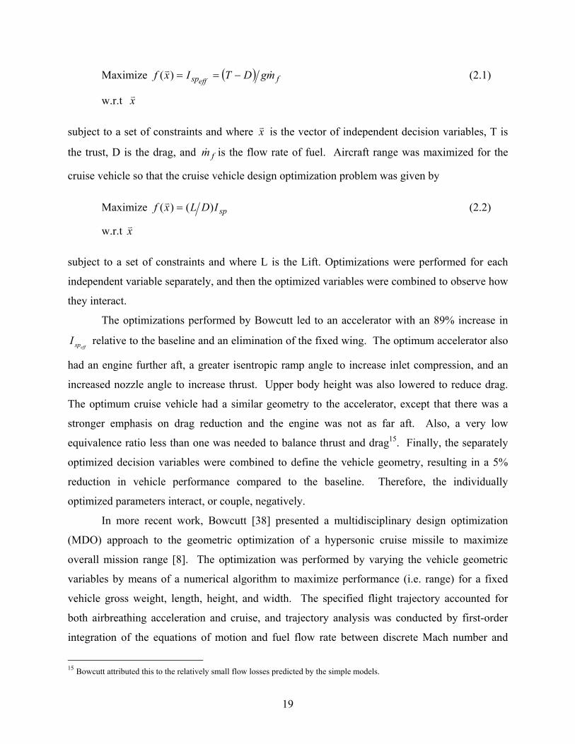
Maximize ( ) fsp mgDTIxfeff

&v −==)( (2.1)

w.r.t xv

subject to a set of constraints and where xv is the vector of independent decision variables, T is

the trust, D is the drag, and fm& is the flow rate of fuel. Aircraft range was maximized for the

cruise vehicle so that the cruise vehicle design optimization problem was given by

Maximize spIDLxf )()( =v (2.2)

w.r.t xv

subject to a set of constraints and where L is the Lift. Optimizations were performed for each

independent variable separately, and then the optimized variables were combined to observe how

they interact.

The optimizations performed by Bowcutt led to an accelerator with an 89% increase in

effspI relative to the baseline and an elimination of the fixed wing. The optimum accelerator also

had an engine further aft, a greater isentropic ramp angle to increase inlet compression, and an

increased nozzle angle to increase thrust. Upper body height was also lowered to reduce drag.

The optimum cruise vehicle had a similar geometry to the accelerator, except that there was a

stronger emphasis on drag reduction and the engine was not as far aft. Also, a very low

equivalence ratio less than one was needed to balance thrust and drag15. Finally, the separately

optimized decision variables were combined to define the vehicle geometry, resulting in a 5%

reduction in vehicle performance compared to the baseline. Therefore, the individually

optimized parameters interact, or couple, negatively.

In more recent work, Bowcutt [38] presented a multidisciplinary design optimization

(MDO) approach to the geometric optimization of a hypersonic cruise missile to maximize

overall mission range [8]. The optimization was performed by varying the vehicle geometric

variables by means of a numerical algorithm to maximize performance (i.e. range) for a fixed

vehicle gross weight, length, height, and width. The specified flight trajectory accounted for

both airbreathing acceleration and cruise, and trajectory analysis was conducted by first-order

integration of the equations of motion and fuel flow rate between discrete Mach number and

15 Bowcutt attributed this to the relatively small flow losses predicted by the simple models.

20

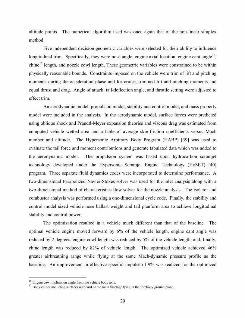
altitude points. The numerical algorithm used was once again that of the non-linear simplex

method.

Five independent decision geometric variables were selected for their ability to influence

longitudinal trim. Specifically, they were nose angle, engine axial location, engine cant angle16,

chine17 length, and nozzle cowl length. These geometric variables were constrained to be within

physically reasonable bounds. Constraints imposed on the vehicle were trim of lift and pitching

moments during the acceleration phase and for cruise, trimmed lift and pitching moments and

equal thrust and drag. Angle of attack, tail-deflection angle, and throttle setting were adjusted to

effect trim.

An aerodynamic model, propulsion model, stability and control model, and mass property

model were included in the analysis. In the aerodynamic model, surface forces were predicted

using oblique shock and Prandtl-Meyer expansion theories and viscous drag was estimated from

computed vehicle wetted area and a table of average skin-friction coefficients versus Mach

number and altitude. The Hypersonic Arbitrary Body Program (HABP) [39] was used to

evaluate the tail force and moment contributions and generate tabulated data which was added to

the aerodynamic model. The propulsion system was based upon hydrocarbon scramjet

technology developed under the Hypersonic Scramjet Engine Technology (HySET) [40]

program. Three separate fluid dynamics codes were incorporated to determine performance. A

two-dimensional Parabolized Navier-Stokes solver was used for the inlet analysis along with a

two-dimensional method of characteristics flow solver for the nozzle analysis. The isolator and

combustor analysis was performed using a one-dimensional cycle code. Finally, the stability and

control model sized vehicle nose ballast weight and tail planform area to achieve longitudinal

stability and control power.

The optimization resulted in a vehicle much different than that of the baseline. The

optimal vehicle engine moved forward by 6% of the vehicle length, engine cant angle was

reduced by 2 degrees, engine cowl length was reduced by 5% of the vehicle length, and, finally,

chine length was reduced by 82% of vehicle length. The optimized vehicle achieved 46%

greater airbreathing range while flying at the same Mach-dynamic pressure profile as the

baseline. An improvement in effective specific impulse of 9% was realized for the optimized

16 Engine cowl inclination angle from the vehicle body axis. 17 Body chines are lifting surfaces outboard of the main fuselage lying in the forebody ground plane.

21

vehicle over the baseline during the acceleration portion of the mission. Finally, trim drag was

lowered by 13% overall.

Research similar to that of Bowcutt has been embarked upon by O’Neil and Lewis [41]

as well as Takashima and Lewis [42]. However, their work focused on optimization with a

different approach to coupled vehicle-airframe problems. They made use of an inverse analytical

method for hypersonic waverider18 design which reduced calculation requirements by using

known flowfields. In the inverse method, desired uniform flowfield conditions at the entrance to

the combustor were specified (the desired shape of the inlet curve was also known), and then

streamlines were traced forward from the inlet curve to the bow shock to produce the shape of

the forebody undersurface that results in the desired conditions. The upper surface was

generated by freestream streamlines traced rearward from the undersurface streamline/shock

intersection. The known generating flowfields in these studies were produced via the method of

osculating cones19.

In general, the component models developed by O’Neil and Lewis and Takashima and

Lewis were essentially the same, with some subtle differences. Two-dimensional planar inlet

ramps were incorporated into the designs with all shocks focused on the cowl lip (similar design

to that shown in Figure 2-1). A variable cowl was assumed to translate at off-design conditions

to maintain both the shock-on-lip condition and shock cancellation at the inlet throat. A quasi-

one-dimensional combustor that included area variation, heat addition, friction, mass injection,

molecular weight variation, and specific heat variation was based upon Shapiro’s influence

coefficients [43] to determine the flow properties. The equations were solved step by step from

combustor entrance to exit using a fourth-order Runge-Kutta technique. The nozzle was

designed for isentropic flow using the two-dimensional method of characteristics and frozen

chemical kinetics was assumed throughout the nozzle. Surface forces were predicted by shock-

expansion theory and also a hybrid of tangent-wedge and tangent-cone methods.

O’Neil and Lewis, like Bowcutt and others, applied the non-linear simplex method as the

optimization scheme. They optimized conically-derived waveriders integrated with scramjet

engines for cruise conditions at flight Mach numbers 8-10 and for acceleration at flight Mach

18 A waverider is essentially any vehicle which uses its own shock wave to increase lift-to-drag ratios and improve overall performance. In these studies, the waverider is considered the forward portion of the vehicle, i.e. upper and lower forebody. 19 In this method, multiple cones are used to design non-axisymmetric shock patterns allowing greater flexibility in the vehicle design. A designer may use varying conical shock shapes for different portions of the vehicle to improve performance.

22

number 10, 12, 14, i.e. the vehicle was optimized for individual mission segments of cruise or

acceleration and not across an entire mission of segments. The parameters that remained fixed

throughout the optimization were flight Mach number, combustor entrance pressure and

temperature, combustor equivalence ratio, and vehicle length, density, and wall temperature.

Fifteen decision design variables were implemented for the cruise optimization and fourteen for

acceleration optimization and were constrained to fall within realistic limits. Behavioral

constraints were also imposed on the vehicle design. The cruise and accelerator vehicles were

optimized by essentially using Equations (2.2) and (2.1), respectively. However, penalties were

included in the objective functions when L = W and T = D were not satisfied for cruise and when

L = W was not satisfied for acceleration.

One result of the cruise optimization was that as the flight Mach number increased, the

vehicle planform shape became more pointed and the upper surface cross-sectional shape

changed from flat for the Mach 8 configuration to more pointed for the Mach 10 vehicle (see

Figure 2.2). Engine size increased with increasing Mach number in order to match the thrust to

drag which, consequently, decreased the lift-to-drag ratio. Other results of the cruise

optimization were a decrease in specific impulse with increasing Mach number and the majority

of vehicle lift was produced by the forebody and outboard20 surfaces of the vehicle. In

comparison with the Mach 10 cruise vehicle, the optimal Mach 10 accelerator had a significantly

larger engine span (i.e. width) and vehicle volume than the optimal cruiser (see Figure 2-2). The

engine was located much farther forward for the accelerator which resulted in a considerable

increase in nozzle length. The primary lifting surfaces for the accelerator vehicles were the ramp

and nozzle (the outboard surfaces were quite small). When comparing all three accelerators, it

was found that all three geometries were relatively similar. However, effective specific impulse

decreased and lift-to-drag ratio increased with an increase in Mach number.

Takashima and Lewis chose to use a sequential quadratic programming method for

optimization. A design was optimized for maximum range along a constant dynamic pressure

trajectory starting from Mach 6 and ending at Mach 10 cruise. For comparison purposes, a

design was also optimized for maximum cruise range for a fixed Mach 10 cruise condition. A

total of eighteen decision design variables were implemented to define the vehicle geometry,

20 In the case, forebody includes the undersurface forward of the ramp and the complete upper surface. Outboard refers to the section of the undersurface outboard of the engine and downstream from the start of the ramp.

23

many subjected to geometric constraints. Both design vehicles were subjected to the same

constraints over the entire mission, including the same initial weight.

Figure 2-2. Representation of the optimal (a) Mach 10 cruise scramjet integrated waverider, (b) Mach 10 accelerator scramjet integrated waverider, and (c) Mach 8 cruise scramjet integrated waverider determined by O’Neil and Lewis [41].

To compare the performance of the two designs, the hypersonic range for the optimized

Mach 10 cruise-range design was calculated along the same trajectory as the optimized total-

range Mach 6-10 vehicle. A significant result of the comparison was that the maximum range of

the total-range vehicle was only approximately 1% less than the maximum range the of cruise-

range design. However, the optimal total-range vehicle covered an 11.5% greater distance

during the acceleration phase and the optimal cruise-range vehicle covered a 2.6% greater

24

distance at the cruise condition. The geometries of both vehicles were relatively similar. The

largest differences were the compression surface lengths, top surface angles, and forebody

angles. A final result, in general, was that optimized accelerators had a greater engine width than

corresponding optimized cruise designs.

The most recent publication (January 2004) in the area of hypersonic vehicle

optimization addressed the issue of system level optimization of high speed tactical weapons.

Baker et al. [44] developed the Integrated Hypersonic Aeromechanics Tool (IHAT) system

which is a multidisciplinary analysis and optimization toolset designed to address the issues of

high fidelity analysis and consideration of interdisciplinary interactions for high speed tactical

weapons. The IHAT system, constructed in multiple builds, addresses many relevant disciplines

important for high speed weapons in an integrated manner. Modules included in IHAT are

geometry, aerodynamics, propulsion, trajectory, thermal, structural, stability and control, sensors,

lethality, and cost index models. The modules are “glued together” using an Integration Core

Module which is responsible for coordinating the execution of the IHAT system and ensuring

that all modules are executed in order and required data is transferred. The four types of IHAT

runs currently supported by the IHAT system are single point analysis, parametric trade studies,

discrete trade studies, and optimization.

The geometry module is responsible for maintaining and updating a parametric geometry

module of the configuration being analyzed. This module includes a finite element mesh used by

the thermal and structural modules, a surface/volume mesh used by the aerodynamics module,

and basic parameters such as volumes and flowpath areas. The aerodynamics module computes

aerodynamic performance of the vehicle over the expected flight mission. The aerodynamics

module implements a variable-fidelity approach with options ranging from simple surface-

inclination methods to complete simulation of the Navier-Stokes equations. The IHAT

propulsion module has the capability of computing propulsive performance of solid rocket

boosters, ramjets, scramjets, dual combustion ramjets, or non-axisymmetric scramjets. The

output of the propulsion module is a database of propulsive efficiency (i.e. thrust, fuel flow rate,

specific impulse) as functions of flight condition and throttle setting. The propulsion and

aerodynamic modules are used interactively to perform trajectory simulation and optimization.

The best overall performance is obtained via the trajectory module once the aerodynamic and

propulsion module are available. Several optimization options are available: minimize fuel burn,

25

maximize range, and minimize time to target. Constraints, such as dynamic pressure and

acceleration limits, may be imposed on the trajectory. The thermal and structural modules are

responsible, respectively, for computing the aerodynamic and propulsive heating environment as

well as the thermal response of vehicle insulation and determining the structural sizing required

for the vehicle to withstand load conditions.

The IHAT system implements nested optimizations, with the most successful being

surrogate-based optimization (SBO). The SBO strategy creates a response surface, i.e. a ‘trust

region’, over a portion of the design space and then applies conventional gradient-based

optimization methods to find the optimum of the approximation. The trust region is then updated

and the process is repeated to convergence.

A sample application was conducted using the IHAT system, more specifically, a system-

level analysis and optimization of the Air Launched Low Volume Ramjet (ALVRJ). The

ALVRJ was a previously built and tested vehicle that incorporated many of the features of a high

speed tactical missile and served as a verification and validation test case. Six decision design

variables were used in the sample application; each constrained to avoid excessively large

perturbations from nominal values. The objective function was a simple weight-based metric

termed the “Weight Margin”. The Weight Margin was essentially equal to the weight of the

payload that could be carried by the vehicle.

The most significant result was an approximate doubling of the weight margin after six

iterations of the global optimization. The weight available for payload was approximately 15%

of total vehicle weight for the baseline vehicle and 30% for the optimized vehicle. The most

significant differences between the baseline and optimized vehicle configuration were that the

optimal vehicle had a smaller booster and ramjet combustor, a longer fuel tank, and a somewhat

reduced diameter.

2.2 Exergy-Based Methods in the Design/Analysis of Hypersonic Vehicles.

The need for a unified framework in the synthesis/design of high performance aircraft

was presented in Section 1.2.It is envisioned that this unified methodology will support all levels

of synthesis/design, lead to innovative configurations which maximize overall system efficiency

26

and minimize energy waste, and ultimately provide a true system-level optimized

synthesis/design. A fair amount of work has made strides towards realizing a unified

methodology for high performance aircraft systems. Specifically, exergy, work potential, and

thrust potential methods have shown much promise in satisfying the aforementioned needs.

Therefore, this section is dedicated to illustrating the usefulness of the methods.

2.2.1 Work Potential/Thrust Potential Methods

The concept of thermodynamic work potential21, based upon the first and second law of

thermodynamics, has been shown to hold promise as a universal figure of merit to gauge the

performance of propulsion systems [9-12, 14, 15, 45]. Unlike conventional component

performance measurements, i.e. component efficiencies, work potential methods applied to

propulsion system performance analysis readily lead to generalized representations of engine

component performance that are directly comparable to one another. Work potential serves as a

basis for developing comprehensive loss accounting systems as well as providing a basis for

relating losses directly to vehicle weight, fuel weight, and cost.

Roth [45] and Roth and Mavris [14, 15], exergy, gas horsepower, and thrust potential

have shown considerable promise as work potential figures of merit for propulsion system design

and analysis. As indicated earlier, exergy is a thermodynamic property which describes the

maximum theoretical work that can be obtained from a system in taking it from an initial state to

mutual stable equilibrium with the environment. Exergy measures loss relative to the absolute

limits of thermodynamics. Gas specific horsepower, on the other hand, is defined by Roth as the

ideal work that would be obtained by isentropic expansion of a high-enthalpy gas to atmospheric

pressure through an imaginary turbine. Gas specific horsepower is a specific case of exergy and

measures losses relative to an ideal Brayton cycle. Finally, thrust potential is defined by Riggins

[9-12] as the overall vehicle net thrust work obtainable if the flow of a high-enthalpy gas at the

station of interest is expanded isentropically to the exit area of the engine. The difference

between each of these figures of merit is in their definition of useful work potential and,

therefore, a loss defined by one figure of merit may not be considered a loss by the other figures

of merit.

21 In general, work potential is the ability of some energy source (energy content of fuel) to produce useful physical work (thrust power). The second law of thermodynamics places an upper bound on the maximum work that can be extracted from a fuel.

27

Roth and Mavris have pointed out that the application of work potential as a tool for

vehicle analysis requires two significant considerations. First, the analysis must be able to

accommodate the wide operating range typical to vehicle operation. Second, the reference

condition for the dead state22 used in vehicular applications must be allowed to ‘float’23. They

attribute these considerations to the fact that most vehicles operate over a wide variety of

ambient conditions and throttle settings when performing their function.

Roth [45] and Roth and Mavris [15] present the general methodology for construction of

detailed loss management models as a four step process. However, an initial step, step “0”,

requires the explicit definition of loss in a way most suited to the analysis at hand, i.e. choose a

figure of merit. The four steps are defined as follow:

1. Identify explicitly all loss mechanisms that are significant to the operation of the vehicle.

2. Create a mathematical representation of each loss source, i.e. develop a differential loss

management model.

3. Integrate the differential loss model through time over a single vehicle mission or duty

cycle to obtain loss chargeable to each loss mechanism.

4. Assign chargeability for each loss to its underlying source.

The first step partitions losses into three general categories: propulsion-chargeable loss, vehicle-

chargeable loss, and work storage mechanisms where vehicle and propulsion-chargeable losses

can be broken down into more specific classes of loss mechanisms according to the desired level

of analysis fidelity. The second step requires application of energy balances in the form of a

thermodynamic cycle analysis to yield the detailed information on the thermodynamic state at

each engine station and operating condition. Second law analysis can be used in conjunction

with the supplied information to determine the work potential at every engine station and

operating condition. Step 3 results in an analytical description of all losses and useful work

transfer occurring in each component of every vehicle sub-system during the vehicle mission.

Finally, step four allocates each loss to the factor(s) that drive it and, therefore, a thermodynamic

cost of each design decision can be understood.

22 Reference state used to determine the value of the exergy, i.e. the state of the “notional reservoir”. 23 This, however, is debatable since the “dead state” is only a reference state which means that the value of “exergy” (or work potential) as any thermo-physical property can only be determined in relative terms, i.e. relative to a given reference state. Thus, the need to vary the “dead state” throughout the mission seems to make little sense from a purely thermodynamic point of view.

28

Roth and Mavris demonstrated the proposed loss management methods on a lightweight

fighter aircraft powered by two J85-GE-21 (gas turbine) engines. In order to demonstrate these

methods, a cycle and installation model of the engines and a mission analysis model were

developed24. The mission considered was a simple subsonic area intercept, consisting of

maximum power take-off and climb, subsonic cruise, combat, and loiter. The figure of merit

chosen to measure loss of thermodynamic work potential for this application was gas specific

horsepower.

During the mission, instantaneous propulsion sub-system and aerodynamic performance

were calculated at every flight condition and the power required to overcome each loss

mechanism was also calculated. The result of this analysis was a set of data tables for propulsion

and aerodynamic losses. These tables displayed the horsepower required to overcome a

particular loss mechanism as a function of altitude and Mach number over the “flight envelope”.

The propulsion sub-system loss plots revealed that inlet losses were only significant at high

Mach numbers and turbomachinery losses were greatest at high dynamic pressure conditions.

Nozzle and afterbody drag losses were also larger at high dynamic pressure conditions. Exhaust

residual kinetic energy was highest at low altitudes and had little dependence on Mach number.

The aerodynamic sub-system loss plots showed contours of power required having a marked

dependence on dynamic pressure and these plots appeared to be qualitatively similar. However,

fuselage wave and skin friction drag and induced drag were the dominant aerodynamic loss

mechanisms. These loss plots provided much useful information because they quantified all

losses, losses which were readily comparable to one another.

When the instantaneous losses were integrated over the entire mission (see Figure 2-3), it

was revealed that total propulsion power loss during climb and combat was much higher than

during cruise. Aerodynamic drag power loss was also greatest during climb and combat.

Residual kinetic energy left in the exhaust stream was by far the dominant gas-specific power

loss during the mission (47% of all losses) (see Figure 2-3). Roth attributed this as a natural

consequence of the thermodynamic cycle on which the J85 engine operates. It was also shown

that the engine component losses decreased in magnitude from the back to the front of the

engine. Finally, it was noted that total loss chargeability’s were equivalent to total fuel mass

24 These models were developed based upon available manufacturer’s published data and using well-known cycle, propulsion installation, and mission analysis tools.

29

chargeability’s because the fuel used to offset each source of loss must be proportional to the loss

in work potential itself.

Figure 2-3. Loss of available gas specific power during F-5E area intercept mission. From Roth and Mavris [15]; reprinted by permission of author’s.

Roth also derived a series of relationships linking classical efficiency-based performance

metrics to modern measures of work potential [14]. The most common component efficiencies

(nozzle gross thrust coefficient, inlet pressure recovery, compressor and turbine adiabatic

efficiency, etc.) were derived in terms of the three previously mentioned work potential

measures. The classical efficiency-based performance metrics were also compared and

contrasted with the work potential figures of merit to highlight the strengths and weaknesses of

each method.

Riggins [11] and Riggins, McClinton, and Vitt [10] pioneered the analysis of scramjet

engines via thrust potential and exergy methods. They developed a method that allowed the

calculation of the lost scramjet engine thrust or thrust potential caused by different loss

mechanisms (i.e. irreversibilities) in one-dimensional or multi-dimensional flowfields and

defined an engine effectiveness parameter to be used in the optimization of engine components.

Riggins argued that the ability of the engine to develop thrust efficiently is the ultimate measure

of engine performance and, therefore, all proposed methods for evaluating scramjet engine

30

performance at high Mach numbers must consequently define an engine efficiency whose

numerator is vehicle thrust or thrust work delivered to the vehicle.

In these investigations, flow losses (irreversibilities) were produced by friction/viscous

effects, shocks, heat diffusion, Rayleigh losses, fuel-air mixing, and non-equilibrium kinetics.

The evaluation of the thrust losses caused by these loss mechanisms was based upon the

principle that the lost thrust work as measured from that of the reversible engine is recoverable

by an additional isentropic expansion of the actual nozzle exit flowfield. This method, referred

to as the lost-thrust method, was applied to engines with uncoupled losses and coupled losses.

However, coupled losses required a complete differential description of the entropy distribution

throughout the engine. It was shown that the lost thrust contributions summed exactly to the

difference in thrust between the reversible flowfield and the actual flowfield. The lost-thrust

method was used to calculate the lost stream thrust by an additional isentropic expansion

utilizing the relation

Rs

e

erirr

eAA ∆

= (2.3)

where e refers to the actual nozzle exit area and er refers to the effective nozzle exit area. For a

known amount of irreversibility and nozzle exit area, Equation (2.3) was applied to determine the

effective nozzle exit area required to recover the lost thrust. Coupled loss mechanisms required

the exit nozzle to be differentially expanded for each separate differential irreversibility increase,

moving from the rear to the front of the engine. The lost-thrust method provided a rigorous

identification and ranking of components in which propulsive losses occurred and also the

engine location of these propulsive losses.

In [10], Riggins, McClinton, and Vitt demonstrated these methods (lost-thrust and thrust

potential) for the analysis of thrust losses in a scramjet engine using a one-dimensional cycle

code with detailed second law (irreversibility) accounting. The analysis was implemented on a

generic hypersonic engine configuration, which include inlet/forebody, combustor, and nozzle, at

flight Mach number 12 conditions and fixed fuel injection conditions. As a result, the actual

thrust potential, the various loss thrust increments, and the ideal thrust potential were plotted (see

Figure 2-4) versus axial engine distance. From this figure, it was evident the incomplete

combustion losses were by far the largest loss mechanism followed by mixing losses. It was also

31

shown that when the thrust losses caused by irreversibilities were added to the actual thrust

potential, the sum recovered exactly the corresponding reversible flow.

Figure 2-4. Thrust potential and losses versus axial distance for engine flowfield. From Riggins, McClinton, and Vitt [10]; reprinted by permission of the American Institute of Aeronautics and Astronautics, Inc.

An overall engine thrust effectiveness parameter was also presented in [10] and was

defined as the ratio of the actual net thrust across the engine to the ideal engine net thrust. The

methods developed in this reference eliminated the need to actually compute a reversible high-

enthalpy flowfield25 and, therefore, evaluation of the ideal engine net thrust was relatively

straightforward. The engine effectiveness parameter was developed to evaluate and compare

scramjet engine thrust performance.

Riggins also illustrated and clarified issues relating to the thrust-potential and exergy

methods (when applied to high-speed aerospace engines) using simple one-dimensional steady

flows with friction, Rayleigh heat addition, and incomplete combustion losses [9, 12]. It was

shown that a conventional exergy-based rational efficiency26 yielded less effective design

information than the thrust-potential method. This was attributed to the fact that the

25 This is based upon slowing the flow reversibly to Mach zero before heat addition. 26 The rational efficiency of an engine component was defined as the ratio of the exergy exiting the component to the total exergy entering the component. This rational efficiency was developed in earlier work by Curran and Murphy [23] as an exergy-based measure of engine performance. However, this measure appears more appropriate for stationary engines than aerospace engines. An exergy-based measure which does work well for aerospace engines, the thermodynamic effectiveness [24], is given in Chapter 6 of this thesis (Section 6.1).

32

conventional exergy method did not account for the degree of nozzle expansion and the open

nature of the Brayton cycle (essential cycle of a scramjet engine). Additionally, an engine-based

exergy27 was developed to account for the open nature of the aerospace engine cycle.

In these references, a component design problem was posed using both the exergy-based

rational efficiency and thrust-potential-based engine effectiveness. The design challenge was to

find the combustor length of a high speed engine (scramjet engine) that optimizes the

performance of the vehicle. A simplified scramjet with a steady flow of air at flight Mach 12

conditions was illustrated in this example (see Figure 6-1). An isentropic inlet and nozzle of

equal area ratios and a constant area combustor with Rayleigh heat addition and high skin

friction were implemented in the model. Although the total energy expended was held constant,

the actual heat released was determined by using an exponential combustion efficiency

distribution. The nature of this function allowed the ongoing friction, at some point, to negate

the benefit of the progressively smaller amounts of heat release and arrive at an optimal

combustor length. The engine effectiveness parameter predicted an optimal combustor length of

0.46 m and was maximized at the engine axial station where the sum of the lost thrust caused by

irreversiblities was minimized. The rational efficiency predicted an optimal combustor length of

0.952 m, approximately twice the length predicted utilizing the thrust effectiveness. The exergy-

based method optimal combustor length also produced approximately 20% less net engine thrust.

A comparison of component losses using the aforementioned methods was performed on

a simple one-dimensional flow (standard air) through a 10-m long constant area adiabatic duct

with friction. The duct was arbitrarily sectioned into an upstream component Y and downstream

component Z, with component Y being one-third of the duct length. Exergy losses and stream

thrust losses were both measured from the duct inflow values. Component Y had a stream thrust

loss of 50.6 N and an exergy loss of 174 kJ/kg. Component Z had a stream thrust loss of 88 N

and an exergy loss of 168 kJ/kg. It was therefore shown that the exergy method did not correctly

rank components (as to largest performance losses) and yielded no useful propulsive

information.

A final measure of the issues involved with assessing component performance losses was

illustrated by revisiting the optimal combustor length problem. The combustor length was fixed

27 Whether or not the quantity so defined is “exergy” is problematic. However, a discussion of the details of this quantity is beyond the scope of this thesis.

33

at 1 m and the combustor was divided into two separate components in a similar manner as the

duct problem. A design problem was to identify the component in which the greatest frictional

losses occurred and then optimize that component by eliminating skin friction within that

component; ultimately seeing which method (rational efficiency or thrust-potential) resulted in a

more optimal engine (greater thrust). Exergy losses caused by friction were greatest in

component Y and thrust losses caused by friction were greatest in component Z. Elimination of

the skin friction within the identified component led to the optimal engines for both methods.

The thrust-potential method produced an engine with 20% more engine net thrust than the

rational efficiency method. This clearly illustrated that the thrust-potential method in

conjunction with the lost-thrust method provided accurate information in terms of identifying

component losses for high speed engine applications, whereas the rational efficiency method did

not.

Riggins, Taylor, and Homan [13] continued and extended work on these methods,

specifically towards the auditing and optimization of high speed vehicles. A theory was

developed for the detailed characterization of high-speed vehicle performance in terms of

irreversibility, combustion, and flow area relief/flow angularity. A full performance audit,

performance losses and gains, was completed in representative scramjet-powered vehicle

simulations. As done in earlier work, it was shown that losses can be stripped out of individual

streamtubes to yield reversible forces and performance lost by a particular component. Some

major findings in this work was that the combustor was the main source of irreversible entropy

production for the entire vehicle, wake mixing cannot be ignored in vehicle optimization, and

vehicle vertical forces are not significantly affected by irreversible entropy production.

2.2.2 Exergy Methods for System-Level Multidisciplinary Analysis

Moorehouse [4] has proposed the need for a unifying framework and a set of metrics to

facilitate system-level analysis and optimization of aerospace vehicles (with focus on hypersonic

vehicles) and suggested that exergy-based methods show potential to do so. It was postulated

that exergy-based methods would allow more complete system integration, manage the

connection of all traditional results into a design framework with a common metric, and permit

explicit trades between dissimilar technologies in a system context. It was also suggested that a

34

minimum exergy destruction solution via system-level analysis should, ideally, be the same as

the more traditional minimum weight solution.

In [4], the development of a systems-level approach for vehicle synthesis/design in

exergy terms is illustrated. It is shown that mission requirements can be stated in terms of work

to be accomplished; and, thus, total mission requirements can be defined as an energy (exergy)

problem. Consequently, each sub-system of a vehicle can be analyzed as a component in finding

the most efficient way to accomplish that work.

Moorhouse illustrated the synthesis/design process by creating a ‘business case’ that the

work to be done is composed of work the customer wants to purchase plus the overhead work.

The customer work is defined as the work necessary to deliver a specified payload to a certain

altitude and velocity and maintain a power supply to accomplish what is required. The rate of

doing customer work is written as

UDPdt

dEW

dtdw

ppw

pc ++= (2.4)

where the first term on the right hand side represents the work required to generate the specific

energy of some payload weight, the second term is the power supply required by the payload,

and the last term is the work to overcome drag chargeable to the payload. The weight specific

energy was defined as the total of kinetic plus potential energies per unit of weight, i.e.

gUhEw 22+= . Integration of Equation (2.4) over a total mission represents the quantity of

work to be considered as a fixed requirement. The overhead work, as defined by Moorhouse, is

the work that has to be done carrying the weight of the vehicle plus the required fuel throughout

the mission.

The rate of doing overhead work is expressed as

DUdt

dEW

dtdw wo += (2.5)

where W is the sum of all vehicle components except for the payload. The customer pays for

both the mission plus the overhead work done, which is accomplished using the exergy of the

fuel burned.

At the system level, the conservation of energy in the time interval dt is shown to be

35

oc dwdwHdW +=−η (2.6)

The energy content per weight of the fuel, H , and the overall system efficiency, η , were

incorporated into Equation (2.6). The overall efficiency introduces consideration of the first and

second laws of thermodynamics as well as that of all components of the vehicle. Moorhouse

explains that Equations (2.4)-(2.6) represent the balance between the work achieved from the

exergy of the fuel and the changes in payload and aircraft specific energy plus the exergy

destroyed to overcome drag, i.e. mission work. The synthesis/design problem posed is to

minimize the overhead work and maximize the overall system efficiency through the use of

exergy as the common currency.

Moorhouse, Hoke, and Prendergast [6] applied these methods (i.e. the exergy process) to

the design of the inlet of a hypersonic vehicle. The addition of a ‘device’ was considered to

maintain the inlet shock focused on the cowl lip to avoid problems of mass spillage or shock

ingestion. The device used the concept of energy addition/extraction with the inlet flow in order

to tailor the Mach number and shock angle. The device was incorporated to avoid the weight

and complexity of a movable inlet system.

In this analysis, a nominal inlet Mach number and ramp angle were specified. Then, for

incoming flow over a range of Mach numbers, the heat input required to achieve the nominal

Mach number was found using Rayleigh line analysis. Thermal energy was exchanged with a

notional thermal reservoir in order to achieve the required heat addition/extraction. The thermal

reservoir was examined for cases of constant temperature and a linear profile (to approximate

ideal heat exchange). The entropy generation rates (exergy destruction rates) were calculated for

both the energy exchange process and the shock process.

From this analysis it was shown that exergy destruction was much greater when thermal

energy shock tailoring was incorporated as opposed to an inlet with no thermal energy exchange.

There was an exergy benefit if the heat exchange process was close to ideal heat exchange. Even

though the no “energy exchange” process had less exergy destruction, the affects of mass

spillage or shock ingestion were not considered in this analysis and would ultimately need to be

taken into account during a complete system analysis. Also, the large changes in the

thermodynamic properties of the inlet flow as a result of energy exchange would need to be

36

considered, i.e. the effects on combustion performance. Finally, the weight consideration of

adding such a device to a vehicle was demonstrated by Moorhouse, Hoke, and Prendergast.

2.2.3 Additional Exergy/Available Energy Research in Advanced Aircraft Analysis

A fair amount of work on exergy methods applied to high performance aircraft analysis

has been presented in the literature. Although many of these works are directed towards specific

vehicle components or systems, the methodologies undertaken and the results of these analyses

have presented valuable insights into exergy methods for aerospace applications.

Ravichandran and Murthy [46] engaged in a generalized available energy analysis of a

scramjet combustor. The performance of a scramjet combustor was established in terms of four

available energy utilization effectiveness parameters based on available energy or exergy.

Ultimately, these parameters were a measure of how well the energy input into the combustor

was converted into the scramjet engine thrust work. One parameter referred solely to the

combustor, while the other three were based on thrust generation by a nozzle attached to the

combustor. Parameters such as combustor entrance Mach number, combustor equivalence ratio,

heat loss fraction, and friction and shock loss fraction were varied to evaluate the trends of the

available energy effectiveness parameters, i.e. scramjet engine performance.

Another analysis of scramjet engines using exergy methods was conducted by Brilliant

[47]. In this work, performance of scramjet systems were predicted using energy balances and

then exergy calculations were performed for the end states obtained from the conventional

anaylsis. Various exergy measures were plotted for the inlet, combustor, and nozzle as a

function of flight Mach number and the trends of these figures were analyzed. Brilliant

attributed a greater understanding of the interactions of the components to the use of the exergy

analysis.

Camberos and Moorhouse [7] have proposed a methodology to incorporate the second

law of thermodynamics into existing computational fluid dynamics (CFD) algorithms. The

objectives included the development of the theoretical framework for calculating local and global

entropy generation rates, entropy-based numerical metrics, and residuals. Also, the approach

taken was to formalize the entropy and entropy generation equation into a form appropriate for

the unstructured Euler/Navier-Stokes solver. The theoretical expressions were to be coded and

then validated and tested by comparing the induced drag of two wing planforms [17]. Camberos

37

and Moorhouse presented an example of the significance of using second law analysis for the

design of planforms. It was stated that classical lifting-line theory predicts that a planform with

elliptical lift distribution will minimize induced drag and recent work has shown that explicit

consideration of entropy generated in the wake shows that a parabolic lift distribution will

minimize induced drag. Also, when using CFD methods, it was emphasized that separation of

the numerical entropy generation from the physical model needs consideration.

Camberos [8] has also worked on quantifying irreversible losses for

magnetohydrodynamic (MHD) flow simulation. The appropriate equations for MHD fluid flow

were first developed and then were supplemented with the entropy and exergy balance equations.

The inclusion of the second law into this complex physical process was to complement and assist

the development of a unified approach to multidisciplinary optimization with minimum entropy

generation (minimum exergy destruction) as the objective function.

Aside from hypersonic vehicle related topics, Figliola, Tipton, and Li [16] applied an

exergy approach to the decision-based design of integrated thermal aircraft systems.

Specifically, both a traditional energy-based approach and an exergy-based approach were

utilized in the design of the environmental control system (ECS) of an advanced aircraft.

Analytical models of the ECS were developed for both methods and compared to assess the

ability of each method to suggest optimal design paths. Multiobjective optimization tradeoff

studies between design weight and entropy generated were used to determine the optimal design

points. As a result, the two analyses provided similar but different decision solutions.

Paulus and Gaggioli [18] have proposed a method for creating overall objective functions

and weighting factors for a light experimental aircraft. Bejan [19, 20] has presented a constructal

theory for the energy systems of aircraft, one example being the derivation of a complete

structure of a heat exchanger for an ECS based upon exergy methods. Others who have applied

work potential and exergy methods to high-performance aircraft are Czysz and Murthy [23],

Curran and Craig [22], and Curran and Murphy [21].

38

Chapter 3

Hypersonic Airbreathing Propulsion Technical Background

The purpose of this chapter is to facilitate and supplement the remainder of the work in

this thesis. The fundamental features of hypersonic flight and hypersonic vehicles along with a

moderately comprehensive vehicle component description and investigation is presented in this

chapter. Relevant equations of compressible fluid mechanics and thermodynamics which will be

referred to throughout this thesis are briefly presented and discussed.

3.1 Fundamental Definitions and Relations

A good place to begin the discussion of the fundamental definitions and equations of

hypersonic flight is a description of the forces acting on an aerospace vehicle in flight.

Figure 3-1 depicts the system of forces acting on the aerospace vehicle as it carries out some

flight trajectory. It is evident from this figure that the instantaneous installed engine thrust (T)

and vehicle drag (D) are parallel to the instantaneous vehicle velocity (V), and the vehicle lift (L)

is perpendicular to the instantaneous vehicle velocity. The weight (W) or gravitational force is

directed towards the center of the Earth. The vehicle flight path angle (θ ) is defined as the angle

between the vehicle velocity and the horizontal.

Application of Newton’s second law of motion along an axis parallel to the instantaneous

velocity multiplied by the instantaneous velocity leads to the following energy balance on the

aircraft:

{ }

+=−

2

2Vdtd

gW

dtdhWVDT (3.1)

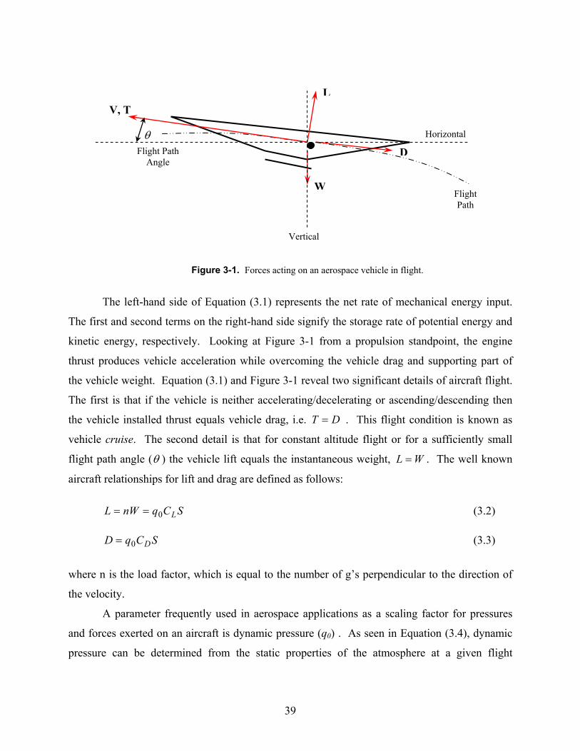
39

Figure 3-1. Forces acting on an aerospace vehicle in flight.

The left-hand side of Equation (3.1) represents the net rate of mechanical energy input.

The first and second terms on the right-hand side signify the storage rate of potential energy and

kinetic energy, respectively. Looking at Figure 3-1 from a propulsion standpoint, the engine

thrust produces vehicle acceleration while overcoming the vehicle drag and supporting part of

the vehicle weight. Equation (3.1) and Figure 3-1 reveal two significant details of aircraft flight.

The first is that if the vehicle is neither accelerating/decelerating or ascending/descending then

the vehicle installed thrust equals vehicle drag, i.e. DT = . This flight condition is known as

vehicle cruise. The second detail is that for constant altitude flight or for a sufficiently small

flight path angle (θ ) the vehicle lift equals the instantaneous weight, WL = . The well known

aircraft relationships for lift and drag are defined as follows:

SCqnWL L0== (3.2)

SCqD D0= (3.3)

where n is the load factor, which is equal to the number of g’s perpendicular to the direction of

the velocity.

A parameter frequently used in aerospace applications as a scaling factor for pressures

and forces exerted on an aircraft is dynamic pressure (q0) . As seen in Equation (3.4), dynamic

pressure can be determined from the static properties of the atmosphere at a given flight

Flight Path Angle

θ

V, T L

D

W

Vertical

Horizontal

Flight Path

40

elevation and knowledge of the velocity or Mach number of the atmosphere as seen from the

moving vehicle such that

22

2000

200

0MpV

qγρ

== (3.4)

The dynamic pressure has proven to be valuable for calculating the forces exerted on

conventional aircraft, specifically the lift and drag (Eqs. (3.2) and (3.3)). It is also effective in

determining forces experienced by hypersonic vehicles with the most popular method being the

modified Newtonian theory [2, 3]. The modified Newtonian theory predicts pressure coefficients

and local surface static pressures of inviscid hypersonic flows through a local surface inclination

method.

The fact that dynamic pressure is a significant parameter in vehicle surface force

determination leads to two critical implications. Structural forces and vehicle drag can become

quite excessive if the dynamic pressure is too large. Secondly, if dynamic pressure is too small,

the wing area required for sustained flight may become unreasonably large. Therefore,

hypersonic vehicles are essentially designed to operate within a fairly narrow range of 0q ,

approximately 2000,90000,20 mN− , and the tendency is to fly the vehicles along the

trajectory of their highest allowable 0q . [1]

Standard day altitudes versus Mach number trajectories for the aforementioned dynamic

pressure design range are provided in Figure 3-2. These trajectories can be generated in a

straightforward fashion by selecting desired combinations of dynamic pressure and Mach

number, using Equation (3.4) to calculate the static pressure, and then obtaining altitude by

interpolation of the table in Appendix B of [1].

There are a few notable attributes of constant dynamic pressure trajectories and

Figure 3-2 worth emphasizing. First, truly enormous flight altitudes would be required for

hypersonic vehicles if it were not for the exponential decrease of static pressure with altitude [1].

Second, freestream mass flow per unit area is proportional to dynamic pressure at a given Mach

number. Therefore, it is imperative that hypersonic vehicles are flown at as high a dynamic

pressure as other considerations will allow in order to maintain mass flow and engine thrust [1].

Finally, if small dynamic pressure trajectories are chosen, the freestream static pressure may be

41

excessively low resulting in unreasonable inlet compression ratios for proper operation of the

combustor. As previously mentioned, small 0q trajectories may also require large wing or

lifting surface areas.

Figure 3-2. Standard day geometric altitude versus flight Mach number trajectories for constant dynamic pressure. From Heiser et al. [1]; reprinted by permission of the American Institute of Aeronautics and Astronautics, Inc.

It is of significance to be aware of the general behavior of air because it is the essential

fluid upon which airbreathing engines depend. Therefore, an issue that is not trivial to

hypersonic flight is the equilibrium behavior of air and the validity of the ideal gas assumption.

The importance of this issue takes affect at high static temperatures and low static pressures, both

of which are commonplace to hypersonic flight.

By definition, an ideal gas is a substance, at relatively high T and sufficiently low P,

which behaves as a single-phase fluid in which each molecule is so weakly coupled to the other

molecules that it hardly experiences their presence [24]. The departure of a gas from ideal

behavior can be estimated from the compressibility factor, where it is customary to use reduced

values of temperature, pressure, and volume in the expression for compressibility factor. It is

proposed that as long as the reduced pressure is less than about 2.0 and the reduced temperature

is greater than about 1.8, the compressibility factor will be within a few percent of unity

(substance exhibits ideal-gas behavior) [1]. In [1] it is suggested that the reduced pressure

42

should never exceed 2.68, the reduced temperature should never be less than 1.64, and the worst

combination of them should never occur due to the nature of the compression process (P and T

increase simultaneously) [1]. Thus, based on known conditions for hypersonic aircraft, it a

reasonable assumption that air behaves as an ideal-gas for the analysis of this thesis.

The significance of the ideal-gas behavior assumption is that specific heats of constant

pressure and volume (consequently, the specific heat ratioγ ) are functions of temperature only.

It also permits application of the ideal gas equation of state, which will be presented shortly.

Figure 3-3 presents the equilibrium ratio of specific heats of air as a function of temperature and

pressure. The figure makes it evident that for the temperature range of air pertinent to this thesis,

ideal-gas behavior is a valid assumption. It also shows that at lower temperatures (below about

500 K), air can be approximated as a perfect gas, meaning specific heats are a weak function of

temperature and are conceivably constant.

Figure 3-3. Equilibrium ratio of specific heats of air as a function of static temperature and static pressure. From Heiser et al. [1]; reprinted by permission of the American Institute of Aeronautics and Astronautics, Inc.

The equilibrium behavior of several major constituents of air as a function of static

pressure and temperature are presented in Figure 3-4. A static pressure of 0.01 atm was chosen

because this is approximately the lowest pressure expected to be found in the hypersonic flight

envelope. Similar results would occur at higher static pressures; however, the higher pressures

merely delay the onset of dissociation of the constituents.

43

Figure 3-4. Equilibrium mole fraction composition for several constituents of air as a function of temperature. Static pressure fixed at 0.01 atm. From Heiser et al. [1]; reprinted by permission of the American Institute of Aeronautics and Astronautics, Inc.

It can be seen in Figure 3-4 that the dissociation of molecular oxygen ( 2O ) into atomic

oxygen (O ) is the principal chemical reaction. It is also evident that the dissociation of

molecular nitrogen ( 2N ) into atomic nitrogen ( N ) as well as the formation of nitric oxide ( NO )

is practically insignificant. For the air temperature range of interest in this thesis work (less than

2000 K), dissociation of air will be assumed irrelevant.

Finally, a presentation of the governing and supporting equations is fundamental to any

analysis. The finite control volume governing equations are presented because this analysis

approach was essential to the thesis work. The governing balances of mass, momentum, energy,

and entropy are given in Equations (3.5) to (3.8), respectively.

∑ ←=q

qmdtdm

& (3.5)

( )∑ ∫∫∫∫∫ ⋅+∀=svc

dAVVVddtdF ρρ

..

(3.6)

∑ ∑

+++++∀−−= ←←←→

k qq

qqqks gz

VhmQQPW

dtdE

2

2

00 &&&&& (3.7)

44

∑ ∑ +++= ←←←

k qirrqq

k

k SsmT

QT

QdtdS &&

&&

0

0 (3.8)

In the above equations, the subscript q refers to any bulk-flow port (inlet or exit) where mass

flow crosses the control volume boundary. The subscript 0 refers to interactions with the

environment and the subscript k refers to interactions with other systems. The left-hand side of

Equation (3.6) represents the sum of all forces acting on the control volume whereas the right-

hand side represents the rate of increase of linear momentum within the control volume added to

the net rate of linear momentum crossing the control volume boundary. In Equation (3.7), the

first and second term on the right-hand side signify the transfer of energy by means of a work

interaction. The third and fourth terms represent the transfer of energy by means of a heat

interaction and the last term denotes the transfer of energy by bulk-flow. It is important to note

that work interactions do not appear in the entropy balance because work involves a transfer of

energy only with no entropy.

Two supporting equations that are utilized frequently in the control volume analysis are

the ideal gas equation of state and the enthalpy relation for an ideal gas, i.e.

RTP ρ= (3.9)

dTTcdh p )(= (3.10)

The equation of state (EOS) is convenient for relating properties at a given equilibrium state.

Equation (3.10) shows that the specific heat at constant pressure and, consequently, the specific

enthalpy are functions of temperature only as well.

Two other equations that are extremely convenient for a point-to-point analysis of

hypersonic flows are that of total temperature and total pressure. The expression for total

temperature and total pressure derived from energy and momentum balances are [3]

−+= 2

211 MTTt

γ (3.11)

45

12

211 −

−+= γ

γγ MPPt (3.12)

where it obvious that they are both strong functions of Mach number. Total temperature is a

fixed property of constant energy flows of perfect gases and total pressure is a fixed property of

constant energy isentropic flows of perfect gases. As will be seen in the next section, changes in

total pressure are directly linked to changes in entropy.

3.2 Shock/Expansion Overview

Shock and expansion processes are quite prevalent during high speed vehicle flight, and it

is, therefore, of utmost importance to have a good understanding of how these mechanisms work

and where and why they arise. It is also critical to understand these mechanisms because the

performance of hypersonic vehicles depends largely upon them, as will be seen in later chapters.

Thus, the following three sections make an attempt to provide a detailed explanation and

discussion of the aforementioned processes.

3.2.1 Oblique Shock Theory

A complete and thorough comprehension of the shock wave process and its ramifications

on flow properties is essential to a study of compressible flow. The shock process represents an

abrupt change in fluid properties in which finite variations in pressure, temperature, and density

occur over a shock thickness comparable to the mean free path of the gas molecules involved

[48]. The shock process itself is adiabatic, thermodynamically irreversible; and mass,

momentum, and energy are conserved throughout the process. Two types of shock waves occur in supersonic compressible flow. The first type is a

normal shock wave which is effectively a plane shock normal to the direction of flow.

Therefore, changes in the flow properties occur only in the direction of flow. The second type

occurs when a compression shock wave is inclined at an angle to the flow direction. This is

referred to as an oblique shock wave. The oblique shock wave process results in a change in

flow direction across the wave. Consequently, a second momentum equation is needed for

derivation of the oblique shock equations. For both types of shocks waves, the shock is assumed

46

thin enough so that there is no area change across the wave [48]. A detailed description of only

the oblique shock wave is given below because it is somewhat more complex and is the

predominant shock wave found throughout the vehicle analysis. Normal shocks are handled in a

very similar fashion.

An oblique shock must occur when a supersonic stream is forced to undergo a finite

change in flow direction into itself due to the presence of a body in the flow and the stream is

unable to gradually adjust to the presence of the body. There are two main types of oblique

shocks referred to throughout this paper. One type occurs during the presence of a wedge in a

supersonic stream (Figure 3-5) and the other is a result of supersonic compression in a corner

(Figure 3-6). For small flow deflection angles, the oblique shock wave remains attached to

either the apex of wedge (Figure 3-5) or to the compression corner (Figure 3-6). The flow after

the shock is uniform and parallel to the body’s surface, with the flow having been turned through

the wedge half-angle or corner deflection angle, both of which are defined by the symbol θ (see

Figure 3-7). These angles are considered synonymous because one can simply imagine the

corner deflection to be a wedge half-angle.

Figure 3-7 provides a more physical representation of the flow characteristics of an

oblique shock wave. As can be seen from this diagram, the upstream (state 1) and downstream

(state 2) velocities are broken down into their components tangential and normal to the oblique

shock. From the geometry of the oblique shock wave and the definition of Mach number,

βsin11 MM n = (3.13)

Figure 3-6. Corner shock

Oblique Shock

Figure 3-5. Wedge shock

Oblique Shock

47

βcos11 MM t = (3.14)

( )θβ −= sin22 MM n (3.15)

( )θβ −= cos22 MM t (3.16)

whereθ is the local flow deflection angle andβ is the oblique shock angle. The deflection angle

and shock angle are related by the θ - β - M correlation (Equation (3.17)) which specifiesθ as a

unique function of 1M andβ , i.e

( ) 22cos

1sincot2tan 21

221

++

−=

βγβ

βθM

M (3.17)

For a known upstream Mach number 1M and deflection angleθ , Equation (3.17) can be solved

iteratively or by using a root finder to calculate the shock angle. The equations of continuity,

momentum, and energy can be written for uniform, supersonic flow over the control surface

indicated by the red dashed lines in Figure 3-7.

Figure 3-7. Oblique shock diagram

The application of these equations leads to two important results, namely, the Mach

number (and velocity) components tangential to the wave are equal, nMM n 21 = , and the total

222 ρTP c.s.

tM 2 nM 2

2MtM1 nM1

1M β

θ

111 ρTP

48

temperature remains constant throughout the shock process, 21 tt TT = . This simply means that

an oblique shock acts as a normal shock for the component normal to the wave. Algebraic

manipulation of the continuity, momentum, and energy equations along with the perfect gas

equation of state leads to relations for the pressure and temperature ratios across the shock as

well as an equation for the downstream normal Mach number as a function of the upstream

normal Mach number [3]. They are

1

12

12

21

21

22

−−

−+

=

n

n

nM

MM

γγ

γ (3.18)

22

21

1

2

1

1

n

n

M

MPP

γ

γ

+

+= (3.19)

22

21

1

2

211

211

n

n

M

M

TT

−+

−+

=γ

γ

(3.20)

With knowledge of the upstream Mach number 1M and deflection angleθ , Equations (3.13),

(3.17) and (3.18) produce the downstream normal component of the Mach number, nM 2 . Thus,

equations (3.19) and (3.20) can be easily solved to obtain the pressure and temperature ratios

across the wave. This process can be repeated for multiple-shock mechanisms with the local

deflection angleθ and shock angleβ measured from the previous deflection angle (surface

angle).

Now, the perfect gas expression for the change in entropy across the shock and an

entropy balance over the control surface gives the irreversibility of the shock process which can

then also be related to total pressure losses across the shock wave, namely,

−

=−=

1

2

1

212 lnln

PP

RTT

csss pirr (3.21)

49

−=

−

1

2ln12

t

t

PP

Rss (3.22)

A few other characteristics of the oblique shock equations are worth mentioning here and

can be seen in Figure 3-8 which shows the variation of shock wave angle with flow deflection

angle for a given Mach number. A more detailed depiction of Figure 3-8 for numerous Mach

numbers can be found in Appendix C of [48].

For a given 1M and θ , two solutions ofβ are possible (as seen in Figure 3-8). There

may be a weak shock, with 2M either supersonic or slightly less than 1, or a strong shock, with

2M subsonic [48]. In both cases, the supersonic flow is turned through the same angle,

however, the strong shock is accompanied by a much larger pressure ratio. When a wedge or

airfoil travels through the atmosphere at supersonic velocities with an attached oblique shock,

only the weak solution is found to occur because large pressure differences cannot be supported

[48].

Figure 3-8. Shock angle versus deflection angle

Another characteristic of the oblique shock equations (also seen in Figure 3-8) is that

large turning anglesθ can produce no solution. These conditions result in a shock that is no

longer attached to the apex of the wedge or the expansion corner as seen in Figures 3-5 and 3-6.

The detached shock is a curve with the shock strength diminishing progressively from that of a

90

β (deg)

250

Strong Shock Solution

Weak Shock Solution

θ (deg)

12=M

50

normal shock at the former attachment point to that of a Mach wave far from the body [48].

Therefore, a detached shock produces the entire range of shock solutions for a given Mach

number. Subsonic flow occurs in the vicinity of the wedge apex or compression corner and

supersonic flow occurs farther back along the wedge or farther out in the flow around the corner.

Due to the non-uniformity of the flow properties, it is highly undesirable to have detached shocks

occur anywhere throughout the hypersonic vehicle flowpath.

Oblique shock reflections and conical shock waves are two other types of supersonic

flow phenomena. The dynamics of these processes will not be discussed here, but further

discussion of these topics can be found in [48]. 3.2.2 Gradual Compressions

As discussed in the previous section, an oblique shock occurs when a supersonic stream

undergoes a sudden change in flow direction. However, supersonic compression in a more

gradual fashion can approach an isentropic process. Allowing supersonic flow to pass through

several weak oblique shocks rather than one strong shock reduces the total pressure losses

(entropy rise) for a given change in flow direction [48]. In the limit, as the number of oblique

shocks gets larger and larger, with each shock turning the flow through a smaller and smaller

angle, the oblique shocks approach Mach waves28 [48]. Therefore, a smooth turn will result in a

continuous compression in the vicinity of the wall. However, the compression waves converge

away from the wall and form a finite oblique shock wave with flow characteristics of those

already discussed in section 3.2.1. A comparison of abrupt compression and gradual compression can be seen in Figures 3-9

and 3-10. These figures will be used to conduct a simple example to evaluate and compare the

final flow properties (Mf, Tf, Pf) as well as the entropy increases for one, two, and three flow

deflections (θ ’s). For all cases, the properties at state 1 are 71 =M , ,1000 21 mNP =

KT 2501 = and the total deflection angle is o12=θ . Application of Equations (3.13) through

(3.21) for the given state 1 conditions along with the aide of Figures 3-9 and 3-10 lead to the

results presented in Table 3-1.

28 Mach waves are infinitesimal disturbances which combine to form shock waves or which individually are capable of producing expansions.

51

Figure 3-9. Abrupt compression of flow.

Figure 3-10. Gradual compression of flow.

It is quite evident from Table 3-1 that as the number of shock increase and the individual

flow deflection angles decrease, the irreversibility (entropy increase) becomes considerably less.

This consequently results in smaller total pressure losses described by Equation (3.22). It can

also be seen that multiple weaker shocks produce a greater final Mach number and pressure and

a slightly lower temperature.

Table 3-1. Gradual compression example results.

Case 1θ 2θ 3θ fM ( )KT f ( )2mNPf ( )KkgJsirr ⋅

1 12 0 0 4.89 466.4 5530 136.1 2 6 6 0 5.13 431.2 5854 40.34 3 4 4 4 5.18 423.8 5943 18.68 4 4 2 6 5.17 426.2 5929 25.09

The results presented in Table 3-1 emphasize why designers of supersonic and

hypersonic inlets would love to have the compression process carried out via isentropic

compression waves. However, it is very difficult to achieve such a compression in real life

because the contour of the compression surface must be quite precise and is only a point design

1θ

1M

fM

1M

1θ2θ

3θ

fM

52

for the given upstream Mach number. Therefore, off-design Mach numbers will result in shocks

for even the best-designed compression contour [3].

3.2.3 Prandtl Meyer Flow

In contrast to oblique shock waves as discussed in section 3.2.1, an expansion wave is

formed when a supersonic flow is turned away from itself. The expansion wave is a two-

dimensional mechanism that typically occurs during supersonic flow over a convex corner or at

the exit of an under-expanded supersonic nozzle [48]. Figure 3-11 depicts an expansion fan

emanating from a sharp convex corner. An expansion fan is simply a continuous expansion

region which can be visualized as an infinite number of Mach waves (weak flow disturbances).

Since the expansion occurs across a continuous succession of Mach waves, and since 0=ds

for each Mach wave, the expansion is isentropic [3]. Also, in contrast to the oblique shock wave,

an expansion fan results in an increased flow velocity and a decrease in pressure and temperature

after the expansion. However, it can be seen in Figure 3-11 that the supersonic flow is still

turned through the local deflection angle θ .

Figure 3-11. Prandtl-Meyer expansion.

Through a geometrical construction of the infinitesimal changes across an infinitesimally

weak wave (in the limit, a Mach wave) and after substantial algebraic and trigonometric

manipulation, the main relationships between flow deflection and Mach number can be

determined and are given in Equations (3.23) and (3.24), namely,

2

2

TP

2M1

1

TP

θ

1M

Expansion Fan

53

( ) ( ) 1tan111tan

11 2121 −−−

+−

−+

= −− MMMγγ

γγν (3.23)

( ) ( )12 MM ννθ −= (3.24)

Equation (3.23) is known as the Prandtl-Meyer function, and it represents the angle through

which a stream, initially at Mach 1, must be expanded to reach a supersonic Mach number M

[48]. It is the key to the calculation of changes across an expansion wave.

For a problem that requires the solution of the properties at state 2 from the known

properties at state 1 and the known deflection angle θ as described in Figure 3-11, a

straightforward analysis procedure is described as follows:

1. For the given 1M , calculate ( )1Mν from Equation (3.23)

2. Using the known θ and the value of ( )1Mν obtained in step 1, solve for ( )2Mν from

Equation (3.24).

3. Obtain 2M through iteration of Equation (3.23) or from tables provided.

4. Total pressure and temperature are constant across the expansion fan because of its

isentropic definition. Therefore, using 1M and 2M the pressure and temperature

ratios can be determined from

1

22

21

1

2

211

211

−

−+

−+

=

γγ

γ

γ

M

M

PP

(3.25)

22

21

1

2

211

211

M

M

TT

−+

−+

=γ

γ

(3.26)

It is evident that, unlike the oblique shock ratios for pressure and temperature (Equations (3.19)

and (3.20)), the normal components of the upstream and downstream are not needed for the

expansion fan pressure and temperature ratio calculation.

A more detailed description of the derivation of Equations (3.23) and (3.24) along with

extensive tables for the Prandtl-Meyer function can be found in [3, 48].

54

3.3 Hypersonic Vehicle and Component Description/Investigation

Before a rigorous discussion of the hypersonic vehicle system and component models is

presented, a general discussion of the major hypersonic components along with synthesis/design

and performance considerations is undertaken. A complete understanding of the geometrical

configuration of the vehicle and components is essential to understanding the behavior of

hypersonic airbreathing engines. This section attempts to provide a portrait of how hypersonic

airbreathing engines operate and of present synthesis/design and performance issues.

It is important to be able to visualize the hypersonic vehicle engine flowpath to properly

understand the distinction between the individual components. A generic representation of the

scramjet propulsion system is, therefore, depicted in Figure 3-12. As seen in this figure and as

mentioned in Chapter 1, the vehicle undersurface operates as the engine, i.e. thrust providing

mechanism. Depending on individual preferences and designs, the propulsion system may

consist of three to five separate sub-systems (the engine cowl is not a sub-system). The three

main sub-systems are the inlet, combustor, and nozzle. The aircraft forebody can be either

included as a propulsion component or be charged to the airframe sub-system (aerodynamics), a

topic of detailed investigation [49-52]. This is attributed to the function of the forebody to

provide pre-compression as well as an adequate amount of vehicle lift. The isolator is usually

disregarded when performing an analysis solely on the scramjet operation of a hypersonic

vehicle. However, it is a significant component of hypersonic vehicles that incorporate the dual-

mode combustion system, i.e. both ramjet and scramjet operation. Although an isolator is not

included in the system models of Chapter 4, a brief discussion of isolator performance is

presented in this section.

. Figure 3-12. Generic propulsion sub-system terminology/components.

5431 2

61 – Forebody 2 – Inlet 3 – Isolator

4 – Combustor 5 – Nozzle/Aftbody 6 – Engine Cowl

Vehicle

55

Efficient operation of the individual components and interactions among the components

displayed in Figure 3-12 are crucial to overall scramjet propulsion system performance. The

combination of forebody and inlet must efficiently compress the air to a suitable Mach number

and pressure to allow for both auto-ignition and effective combustion of the fuel. The inlet must

accomplish all of this all while providing uniform combustor entrance flow (as uniform as

possible) and avoiding high static temperatures. Depending on injector location, non-uniform

flow to the combustor may cause ignition problems. Excessive static temperatures can result in

the onset of dissociation (see Figure 3-4), which significantly reduces the combustion heat

release [21]. A lower static temperature can be generated while achieving a desired static

pressure level by utilizing a more efficient compression process composed of mainly isentropic

turning and weak shocks. In contrast, a compression via stronger shock waves is much less

efficient and thus results in greater static temperatures. For a given static pressure, entering the

combustor at a lower static temperature ultimately produces a lower combustion temperature and

consequently less chemical dissociation occurs [21]. However, it should not go without saying

that too low of a combustion temperature can have negative effects on the auto-ignition of the

fuel. Any dissociation that may occur could, ideally, be recombined to recapture the dissociation

energy by means of an equilibrium expansion process. Conversely, hypersonic vehicle

synthesis/designs generally require rapid initial area expansion, producing a rapid decrease in

static pressure freezing any chemical processes [21]. The dissociation energy is therefore lost

from the propulsion cycle, and, thus, the net thrust is reduced [21].

3.3.1 Inlet Compression and Isolator Components

The goal in the design of any hypersonic inlet is to provide an efficient compression

process, deliver nearly uniform flow and desirable static properties to the combustor, generate

low drag, and provide these characteristics over a wide range of flight and engine operating

conditions [21]. Due to the wide range of flight conditions to be encountered, the chosen

configuration must simultaneously satisfy numerous interrelated and sometimes conflicting

design requirements. The design of hypersonic inlets is greatly influenced and complicated by

vehicle and flight constraints - i.e. mass capture and contraction limits, starting limits, boundary

layer separation, and others.

56

Once again, a physical representation of some typical inlet geometries is imperative to

understanding compression component analysis. Two common configurations are depicted in

Figures 3-13 and 3-14. Figure 3-13 demonstrates an inlet compression system that is solely

comprised of external oblique shock waves. The internal flow downstream of the final oblique

shock is uniform and parallel to both the vehicle and engine cowl. A mixed external and internal

oblique shock wave system, shown in Figure 3-14, is employed to achieve desired combinations

of compression and flow turning. In contrast to external compression systems, mixed

compression systems can result in configurations with the cowl parallel to the freestream flow

and, generally speaking, allow a system of weaker shocks. An ideal compression system would

be that of a continuously curved surface that results in infinitesimal compression waves (Section

3.2.2), culminating with isentropic pressure increase. Other configurations include inlet

sidewalls and strut-like structures. A more detailed explanation of inlet configurations can be

found in [1, 21].

Figure 3-13. External oblique shock wave compression component.

Figure 3-14. Mixed external and internal compression component.

Cowl

Vehicle

Oblique Shock Waves

Streamlines M0

Cowl Oblique Shock Waves

Streamlines

Vehicle

M0

57

It should be evident that understanding oblique shock characteristics is imperative

because they provide the main mechanism for compression. An important design trait of a

hypersonic inlet is the ‘shock-on-lip’ condition. As shown in Figures 3-13 and 3-14, the external

oblique shock waves are ‘focused’ on and terminate at the lip of the engine cowl. This condition

permits 100% mass capture, avoids flow spillage, and prevents shock ingestion. Shock ingestion

could be detrimental to effective combustion and, thus, should be avoided at all costs. Flow

spillage may be either beneficial or detrimental, depending on engine operating conditions.

Given that hypersonic engines operate over a large flight envelope, compression systems

seldom operate at their synthesis/design point. Inlets operating at ‘off-design’ require means of

controlling and tailoring oblique shocks to avoid unfavorable flow conditions. To some degree,

this can be accomplished through a variable-geometry compression system. However, the large

operating range inhibits its effectiveness. Therefore, additional means of controlling the inlet

shock system are necessary, i.e. thermal energy exchange with flow, off-cowl energy deposition,

or MHD29.

Work by Moorhouse, Hoke, and Prendergast [6] demonstrated the use of a thermal

energy exchange with the inlet flow in order to tailor the inlet shock position and maintain an

inlet design Mach number under off-design conditions. This simplified methodology is

employed in this thesis work (see Chapter 4) because it readily adaptable to one-dimensional

analysis. The maintaining of an inlet design Mach number allows the satisfaction of the ‘shock-

on-lip’ condition for fixed geometries over the entire flight range. However, the energy

exchange may cause unsatisfactory changes to the freestream static pressure and temperature.

This issue will be touched upon further in the individual component models of Chapter 4.

Extensive research has been performed on off-cowl local energy deposition and MHD

sub-systems [53]. Local energy deposition in essence creates a heated region upstream and

slightly below the cowl lip, thus, elevating the region’s temperature and pressure. This results in

inlet flow deflection and increased mass flow capture, creating a ‘virtual cowl’. The possible

mechanisms of energy addition are plasmas, laser or electron beams, microwave energy, etc.

[53]. MHD generated power can also be used to create a ‘virtual cowl’ that would increase mass

capture and possible engine thrust. One use of MHD generated power would be to extract

29 Magnetohydrodynamics is the study of the interaction of a magnetic field and an electrically conducting fluid. It can be also defined as the study of plasma motion and dynamics in the presence of a magnetic field.

58

energy from high temperature regions downstream of the combustor and add that energy

upstream of the inlet to optimize inlet performance [53]. These methods of shock system control

are far from trivial and are practically impossible to model in a one-dimensional analysis.

Therefore, even though energy addition/subtraction for creating the virtual cowl are used in this

thesis work, the methods used to practically achieve this are not considered.

Mass Flow Capture

Inlet mass flow capture is vital to engine operation and overall hypersonic vehicle

performance. As previously stated, 100 % mass flow capture occurs at the ‘shock-on-lip’

condition. When inlets shocks stand out in front of the cowl lip, mass flow escapes under the

cowl and the engine is not operating at 100 % mass flow capture. This phenomenon, known as

spillage, is demonstrated in the inlet of Figure 3-15. Spillage is defined as the difference

between the airflow that could pass through the area obtained by projecting the end point of the

cowl lip axially to the freestream flow, referred to as 1A , and the throughflow area of the

freestream flow 0A that actually enters the physical opening [19]. The spillage in Figure 3-15 is

therefore 01 AA − .

At large hypersonic flight altitudes where the density is quite low, mass flow spillage

may be highly undesirable. Mass flow spillage may also be undesirable during hypersonic

acceleration where thrust requirements are rather large. Higher density, lower flight altitudes

may require some spillage, but it does not go without a penalty. Mass flow spillage results in

additional drag around the spillage area and, therefore, higher than necessary equivalence ratios30

may be required in the combustor in order to produce the extra thrust to compensate for the drag.

Accurately predicting and calculating mass flow spillage in the context of one-

dimensional analysis can be difficult. Consequently, the modeling done in this thesis work aims

at maintaining the ‘shock-on-lip’ condition at all flight conditions for 100 % mass flow capture

and is done so via means described in the individual component models of Chapter 4.

30 The equivalence ratio is defined as the ratio of the actual fuel-to-air ratio to the stoichiometric fuel-to-air ratio. It is commonly used to indicate quantitatively whether a fuel-oxidizer mixture is rich, lean, or stoichiometric.

59

Figure 3-15. Mass flow spillage and area definitions.

Inlet Flow Starting and Contraction Limits

Scramjet inlets must operate in started mode for proper operation of the vehicle. Starting

limits refer to the degree of acceptable internal contraction that an inlet may possess to ensure

that the flow phenomena in the internal portion of the inlet do not alter the capture characteristics

of the inlet. An inlet will self-start at a certain internal contraction depending upon the

freestream conditions and the inlet geometry. With use of Figure 3-15, the inlet internal

contraction ratio is defined as 32 AA where 2A is the area between the vehicle undersurface and

the cowl lip and 3A is the area at the inlet throat. Preliminary estimates of the internal

contraction ratio that will self-start can be approximated by the Kantrowitz limit given by [21].

)1(2

1

21

222

111

22

1

22

22

23

2 1

)1(21

2)1()1(1 −

+

−−

+

−+

−−

+

+−

+=

γγ

γγγ

γ

γ

γγγ

γγ M

MMM

MAA

Kantrowitz(3.27)

2M here is the Mach number of the inlet flow where internal contraction begins. Although not

immediately evident from Equation (3-27), the allowable starting contraction ratio increases as

Mach number increases. Experimental data suggest that the Kantrowitz limit becomes

conservative at higher Mach numbers and internal contraction ratios as high as 2 to 3 can be

tolerated [21].

An inlet can be unstarted either by overcontracting to the point where the flow chokes at

the inlet throat, having sufficiently distorted flow at the inlet face, or by raising the back pressure

M0

Streamlines

2A

3A

1A 0A Vehicle

60

beyond the level that can be sustained by the inlet [21]. When inlet unstart occurs, boundary

layer separation may occur, creating undesirable flow characteristics. Mass flow spillage may

also occur, depriving the engine of the airflow necessary for thrust. Finally, fuel control systems

may be unable to properly adjust to the rapidly changing combustor entrance conditions [1]. For

these reasons, inlet unstart must be avoided by any means necessary.

Since overcontraction is an area of concern, correlations for maximum contraction ratios

have been developed via experimental analysis. The contraction ratio is defined as, with the aid

of Figure 3-15, the ratio of freestream capture area to the inlet throat area, 30 AA . An empirical

fit to experimental data is given in [21] as

2000

3 65.352.005.0MMA

A+−= (3.28)

and is applicable to the Mach number range of 105.2 0 << M . Non-uniform flowfields at the

inlet throat have an affect on the maximum contraction ratio; and, thus, the inlet throat profile

should be as uniform as possible to operate at high contraction ratios.

Boundary Layer Friction and Separation

The development of the boundary layer within an inlet substantially affects the overall

performance and operability of the inlet at hypersonic speeds [21]. The boundary layer serves as

an additional compression mechanism of the captured flow, along with oblique shocks and area

change. Issues briefly addressed are that of boundary layer friction and separation.

Friction within the boundary layer provides viscous dissipation of the flow and, therefore,

a loss mechanism with which it must be reckoned. However, rigorous modeling within the

framework of one-dimensional flow cannot be done. Heiser and Pratt [1] employs a method of

separating out the oblique shock wave system analysis from the frictional analysis and a method

somewhat similar to that is used in the system models of Chapter 4. Experimental studies have

shown that viscous compression at leading edges is appreciable at hypersonic speeds. However,

it is not as significant as the other mechanisms previously discussed [21].

Boundary layers are subjected to high adverse pressure gradients due to the desire to

compress the captured air in a relatively short length. These adverse pressure gradients adjacent

to the vehicle surfaces, stemming from oblique shock waves, may cause separation, depending

61

on shock and boundary layer strength. The main mechanism for separation is that the cumulative

upstream viscous forces have dissipated the momentum necessary for the boundary layer to

overcome the imposed pressure rise [1]. Boundary layers more than likely will reattach with the

consequence of a region of reversed and recirculating flow and a zone of high heat transfer near

the reattachment point. Turbulent boundary layers can sustain much larger pressure gradients

and are, therefore, more resistant to separation than laminar boundary layers. Turbulent

boundary layers, unfortunately, increase frictional losses and heat transfer. Therefore, it is

highly desirable to design an inlet knowing where boundary layer transition will occur.

An increase in drag, much stronger than skin friction drag, is another consequence of

separation. The separated region is unstable with large distortion which can lead to flow

blockage and uncertainty downstream of the separation. These undesirable characteristics of

separated flow are just a few reasons why boundary layer separation should be avoided on

hypersonic vehicles.

Inlet Isolator

Isolators are needed during the low Mach number (ramjet mode) portion of the flight

regime where subsonic combustion is expected. Isolators are usually constant area ducts that

contain a shock train (normal or oblique) to provide a mechanism for a supersonic flow to slow

to subsonic speeds and adjust to a static back pressure higher than its inlet static pressure. They

also contain the high pressure produced by the large pressure rise in the subsonic combustor and

prevent inlet unstart. Shock trains in constant area ducts have the characteristic that the

maximum static pressure rise they can generate is exactly the same as that which would exist

behind a normal shock wave at the inlet throat [1]. The synthesis/design and operation of a dual-

mode scramjet requires an isolator at low speeds without penalizing scramjet performance at

hypersonic speeds.

Inlet Constraints and Performance Measures

In addition to being able to address the wide array of synthesis/design issues, the

hypersonic vehicle inlet is subject to constraints for proper operation of the scramjet engine. The

main constraints imposed on the inlet are restrictions on the flow static conditions at the inlet

exit/combustor entrance. Suitable pressures and temperatures are necessary for auto-ignition of

the fuel in the combustor and to provide reasonable combustion reaction rates. If the pressure

62

and temperature are too low, the length of the combustor required to complete the reaction and

consume the available fuel will be excessive. Curran and Murphy [21] and Heiser and Pratt [1]

suggest a commonly applied rule of thumb of 0.5 atm. for the minimum pressure and 10 atm. for

the maximum at the inlet exit/combustor entrance interface. However, it is highly unlikely that

inlet exit pressures will ever be anywhere near the maximum allowed value because compression

to rather high pressures would almost certainly cause the inlet flow to go subsonic. These same

researchers state that a minimum temperature of 1100 K must be provided by the inlet to ensure

auto-ignition and a maximum of approximately 1700 K to prevent excessive dissociation in the

exhaust flow. Other literature references [41, 54] assert pressures between 0.25 – 1 atm. and

temperatures in the range of 1000 to 2000 K must be provided to the combustor by the inlet

compression system. Other constraints are the starting and contraction limits already discussed

and flow turning restrictions to prevent boundary layer separation.

There are an abundance of parameters that have been formulated for the quantitative

evaluation of compression component performance, each with its own rational. Three of the

more accepted and more widely applied of these in hypersonic compression systems are total

pressure ratio, kinetic energy efficiency, and adiabatic compression efficiency which are

expressed as

1

20

23

0

3

211

211

0

3

−

−+

−+

==

γγ

γ

γ

πM

M

PP

PP

t

tc (3.29)

2

0

2exp

V

VidealKE =η (3.30)

( )

−

−−−=

11

211 2

0 ψηγη KE

c M (3.31)

The total pressure ratio is defined as the ratio of the total pressure at the entrance to the

combustor divided by the total pressure of the freestream flow. The kinetic energy efficiency is

defined as the ratio of the square of the velocity that the compression system exit flow would

achieve if it were isentropically expanded to the freestream static pressure to the square of the

63

freestream velocity [1]. Kinetic energy efficiency is a direct measure of the preservation of

kinetic energy, the most important quantity in scramjet propulsion for thrust production. The

kinetic energy efficiency is near 1 at most large Mach numbers; therefore, at least three

significant figures are needed to insure acceptable accuracy. Finally, it is shown in Equation

(3.31) that the adiabatic compression efficiency is a function of the flight Mach number, kinetic

energy efficiency, and ψ , which is the inlet static temperature ratio.

3.3.2 Combustion Component

The development of a hypersonic vehicle utilizing air-breathing engines suggests the

injection and burning of hydrogen fuel in a supersonic airstream and a thorough understanding of

the means by which this can be accomplished. Supersonic combustion is preferred at increased

Mach numbers because higher levels of performance can be attained. The primary function of

the combustor is to burn the fuel in order to release energy to the flow, which can then be

expanded via the nozzle to produce vehicle thrust. The combustion of the fuel may take place in

constant area ducts or ducts with some area relief (divergent sections) to prevent the thermal

choking of the flow. The effects of reaction and heat release from combustion at greater

hypersonic Mach numbers are less pronounced than at lower hypersonic Mach numbers. The

energy from heat release may be only a relatively small portion of the total enthalpy of the

working fluid at higher hypersonic Mach numbers whereas at lower hypersonic Mach numbers

the kinetic energy of the air and the potential combustion heat release are roughly equal [21].

Large heat loads occur in the combustor at hypersonic velocities; and, therefore, a

thermally balanced combustor is required to avoid material limits. The main mechanism used

for combustor wall cooling is to circulate fuel behind the walls and allow the fuel to act as a heat

sink. Thus, fuel injection characteristics are directly determined by system cooling requirements.

Allowing the coolant to be raised to its highest possible temperature without avoiding material

limits makes best use of each unit of coolant. The more thermal energy each unit of fuel used as

coolant can absorb, the less likelihood of having to ‘waste’ fuel because the equivalence ratio

exceeds 1 [1]. One benefit of using hydrogen as the fuel is that hydrogen is far superior as an

engine coolant to typical hydrocarbon fuels because of its ability to absorb more energy per unit

mass. Another benefit is that hydrogen’s large energy release per unit mass, kgkJ954,119 ,

offers the potential of flight to freestream Mach numbers of 15 and beyond. There are a few

64

disadvantages of using hydrogen as a fuel as well. The low density of liquid hydrogen requires

large storage tanks and storage of liquid hydrogen is accomplished through cryogenic systems

that are often costly and quite complex.

The combustion component tends to be the one in the hypersonic vehicle with the largest

destruction exergy, i.e. flow losses. Consequently, combustion system synthesis/design has the

greatest impact on vehicle performance over the vehicle’s operating range. Flow losses

occurring in the combustor arise from fuel-air mixing, non-equilibrium chemical kinetics,

injector and wall drag, and heat transfer across a finite temperature difference. Accurate

methods of predicting these losses and their individual effect on hypersonic propulsion and thrust

production are of the utmost importance.

Optimal combustor synthesis/designs are based, as a minimum, on the engine thrust

potential [21]. The concept of thrust potential was presented and more thoroughly discussed

earlier in Section 2.2.1. Briefly, thrust potential is the thrust generated by an ideal expansion of

combustor exit conditions. It is often non-dimensionalized by an ideal thrust to form an

effectiveness parameter which in turn can be used for engine analysis and synthesis/design. For

example, the effectiveness parameter can be implemented to compare competing fuel injection

concepts or to determine optimal combustor lengths.

Fuel Injection and Fuel-Air Mixing

The efficiency and effectiveness of fuel injection to a large degree determines the net heat

release achieved in scramjet combustion [21]. The extent of fuel-air mixing achieved reflects the

efficiency while a more effective injection strategy translates into a greater thrust potential, i.e. a

minimization of combustor exit streamthrust losses incurred during mixing. The combustion

efficiency is critically related to the degree of fuel-air mixing and ultimately the feasibility of

hypersonic propulsion. Therefore, it is advantageous to understand some fundamental

implications of the various fuel injection strategies and their associated benefits and

disadvantages.

A wide array of fuel injection strategies have been proposed and examined throughout

the literature [1, 21, 55-57]. A few of these strategies have also been studied to predict mixing

efficiency and the losses associated with mixing and their inherent affect on thrust potential [56,

57]. A few injection/mixing techniques are parallel stream mixing, normal fuel injection via wall

jets, and in-stream injectors (e.g., angled ramp injectors).

65

The mixing of air and fuel in parallel streams is one injection technique proposed for

scramjet engines. The fuel and air velocities can either be equal or of different magnitude. If the

velocities are equal there is no lateral transport of momentum and only a lateral transport of mass

due to molecular diffusion. Unequal velocities in the two streams produce mass transfer through

diffusion and lateral momentum transfer from the faster to the slower stream, resulting in a shear

and mixing layer. Although parallel injection is beneficial in terms of fuel momentum addition,

it results in non-efficient mixing and unreasonably long combustor lengths. A further increase in

the velocity difference between the two streams can reduce convective times and axial distance

required for mixing to be completed [1]. However, detrimental consequences such as increased

drag and viscous dissipation are more than likely to occur. In the end, shear layer mixing

(parallel streams) cannot meet the stoichiometric requirements for optimal combustion [1].

Mixing with normal fuel injection by means of wall jets is another technique investigated

for scramjet propulsion. Normal injection minimizes intrusion in the combustor flowpath and

increases local mixing of fuel and air but, unfortunately, creates a relatively complex flow

structure in the vicinity of the jets. A detached normal shock wave forms just upstream of the jet

and, as a result, leads to boundary layer separation [1]. Inherently, total pressure losses arise

from the normal shock wave and boundary layer separation which lead to a decrease in overall

cycle efficiency. Normal injection reduces the mixing transition distance, i.e. ‘jump-starts’ the

mixing, and causes a greater initial growth of the mixing efficiency but weakens the far-field

mixing characteristics in such a way that approximately the same length combustor is required

for complete mixing as with the parallel configuration [1]. An increase in efficiency may

possibly be realized through an optimization of wall jet injection angle and jet spacing.

A final injection strategy examined is in-stream injection, usually31 through axial vortex

mixers termed hypermixers. The design objective of these devices is to create axial vortices32 to

sweep through and entrain the central fuel jet, successfully leading to enhanced near-field and

downstream mixing and lower total pressure losses. Fairly recent research has shown that the

addition of streamwise (axial) vorticity in supersonic flow can increase mixing rates, as much as

sixty percent [1]. One typical type of hypermixer is that of wall-mounted inclined ramps aligned

with the flow, i.e. injectors pointing downstream. These configurations make use of an oblique

31 Other in-stream injection techniques have been investigated such as strut-like injectors with configurations similar to the wing/airfoil geometry of conventional aircraft. 32 This is in opposition to lateral vortices, which are the predominant vortex structures found in parallel and normal fuel injection.

66

shock or expansion fan to produce the necessary axial vorticity. A significant increase in the

near-field, fuel-air mixing and combustion has been shown in a study comparing near-field

mixing for a parallel-injected jet with and without passage of the jet through an oblique shock

[1]. Although there may be a gain in mixing enhancement, it should not be overlooked that an

additional total pressure loss occurs due to the oblique shock.

After examination of the various mixing strategies, it should be apparent that shear layers

created by parallel injected streams and the use of lateral vortices cannot sufficiently achieve

near-field mixing to required stoichiometric proportions of air and hydrogen. However, valuable

insights and concepts have been clarified that may be utilized in future work.

Dual-Mode Combustion Component

As noted in Chapter 1 of this thesis, sustained flight over a large range of Mach numbers

requires hypersonic vehicles to be able provide subsonic combustion for flight Mach numbers

less than about 5, and supersonic combustion for flight Mach numbers greater than about 6 or 7.

For this to be achieved and to avoid having to carry two different engines, it is desirable to have

subsonic flow, when necessary, in the combustor without area constrictions either upstream or

downstream of the burner33 as required by a purely ramjet engine. Heiser and Pratt [1] credits

E.T. Curran and F.D. Stull with developing the concept of a dual-mode combustion system in

which both subsonic and supersonic combustion can be made to occur within the same scramjet

engine geometry.

When operating in ramjet mode, the flow is made subsonic at the combustor entrance by

means of the isolator, which has already been described in Section 3.3.1. Instead of two physical

throats, a choked34 thermal throat is provided by the dual-mode combustor which thereby chokes

the flow and fixes a large burner entry back pressure [1]. This back pressure produces a normal

shock train to form in the isolator and, therefore, results in subsonic flow delivered to the

combustor. The choked thermal throat is brought about by choosing the right combinations of

area distribution, fuel-air mixing, and combustion [1]. This thermal throat also allows the

subsonic flow to be accelerated to supersonic velocities.

Since in scramjet mode the desired flow is to be supersonic at the combustor entrance,

there is no apparent need for an inlet isolator. Even though the flow anywhere within the engine 33 Burner and combustor are used synonymously throughout this discussion. 34 Choked refers to conditions in the flow where the Mach number equals one, M = 1.

67

is ideally neither choked nor subsonic, if the area increase in the burner is not sufficient to relieve

the thermal occlusion resulting from heat addition to a supersonic stream, an adverse pressure

gradient arises [1]. Boundary layer separation may occur as a result of these pressure gradients

which allow the pressure rise to propagate upstream and, if not contained, cause engine unstart.

This phenomenon can be contained once again through the isolator.

Transition between these two operating modes (ramjet and scramjet) adds further

complexities to the design of dual-mode combustion systems. General one-dimensional analysis

of dual-mode systems has led to the conclusion that a constant area combustor in conjunction

with a constant area isolator is not a good combination for these configurations [1]. Instead, a

burner with some area relief (increasing area) coupled with a constant area isolator provides the

means to allow a useful operating range for mode transition [1].

3.3.3 Expansion Component

The expansion component, i.e. the nozzle, functions to expand the high pressure and high

temperature gas mixture exiting from the combustor to local atmospheric pressure and accelerate

the flow to high exit velocities to generate thrust35. Potential energy is converted to kinetic

energy during the expansion process and the shape of the expansion component determines the

angle of the gross thrust vector relative to the vehicle’s flight direction. Two important factors of

hypersonic nozzle design are efficient generation of thrust and the aerodynamic stability of the

vehicle. These issues are significant because the nozzle ‘works’ on the total flow through the

engine and the high surface pressure forces and thrust direction encompass a substantial portion

of vehicle trim [21].

Performance of the expansion component is influenced by the loss mechanisms occurring

in the component. The main loss mechanisms found in expansion components are skin friction,

heat loss, failure to recombine dissociated species, and flow divergence and under-expansion

losses. The most complex loss mechanisms are dissociation losses, which result from the flow

freezing in the rapid expansion process and consequently prevent energy addition by the

recombination of free radicals produced by the combustion process [21]. Dissociation tends to

be more prevalent at higher Mach number flight where combustor exit static temperatures are

usually higher. Therefore, it is easy to see that dissociation losses are directly related to the 35 Moreover, it functions to capitalize on the thrust potential of the flow leaving the combustor.

68

efficiency of the compression component. Skin friction and heat transfer are much larger in the

first half of the nozzle, therefore, it would be beneficial to form laminar flow within this region

to reduce both of these losses. Flow divergence losses are a result of the streamlines at the

nozzle exit being at different angles relative to the flight path and under-expansion losses arise

by not expanding the flow to ambient pressure. Nozzle performance can be very sensitive to

both of these last two design consideration [21].

One typical measure of nozzle performance is the gross thrust coefficient, sometimes

referred to as CFG. It is defined as the actual gross thrust of the stream tube at the exit plane of

the nozzle divided by the equilibrium ideal thrust of the flow-path stream tube expanded to the

local atmospheric pressure [1, 21]. A well-designed nozzle would have a gross thrust coefficient

of about 0.96, with a practical upper limit of about 0.97 [21]. Other performance measures are

the total pressure ratio, Equation (3.29), as well as a parameter similar to the kinetic energy

efficiency termed the velocity coefficient. The velocity coefficient is simply the ratio of the

actual average total velocity at the exit of the expansion sub-system to the ideal total velocity [1].

Due to the tight integration of the airframe and engine, hypersonic vehicles

synthesis/designs use two-dimensional expansion as opposed to axisymmetric or circular

expansion. A reason for this is because circular nozzles are comparatively heavy and are not

easily adaptable to variable geometry [1]. Also typical of hypersonic scramjet engines, optimal

exhaust areas are approximately 1.5 to 2.0 times the freestream engine capture areas [21]. A

final nozzle design constraint is that the initial nozzle expansion is limited to a maximum value

of somewhere around 18 degrees [58-60].

Although expansion components are simpler than other vehicle components in the sense

that the number of synthesis/design requirements to be met are fewer, their performance

throughout the entire flight regime is very important to overall vehicle system performance.

69

Chapter 4

Comprehensive Sub-system and Component Models

Realistic component models are necessary to adequately describe the flow physics and

predict the performance of a hypersonic vehicle over a rather large range of operating conditions.

Therefore, an appreciable amount of time was dedicated to developing and validating the

individual component models presented in detail in this chapter. A variety of analysis techniques

were utilized throughout the model development, ranging from simple geometric relations to

oblique shock and Prandtl Meyer expansion theories to more advanced differential ‘marching’

schemes. The objective of this chapter is to provide a rather rigorous description of the

hypersonic vehicle systems and sub-systems and the equations governing the analysis.

4.1 Propulsion Sub-system Description

The propulsion sub-system of a hypersonic vehicle, as noted in Chapter 3, is comprised

of three main components; specifically the inlet, combustor, and nozzle. This analysis excludes

an isolator model because the hypersonic vehicle undergoes supersonic combustion at all

operating conditions, i.e. ramjet operation omitted. The propulsion sub-system components are

presented in the manner in which flow proceeds through the engine. A sufficient number of

figures are included to provide a more detailed physical representation of components, analysis

methods, etc. and to supplement the discussion that follows.

4.1.1 Inlet Component Description and Modeling

A mixed external and internal compression component is implemented to model the inlet

component. The main mechanism for compression, as noted in Chapter 3, is a direct result of the

oblique shocks produced from flow turning. Skin friction drag is included on the vehicle inlet

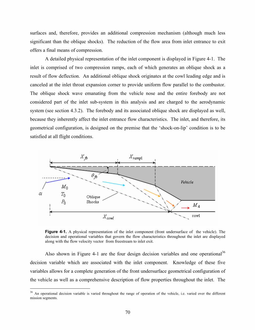
70

surfaces and, therefore, provides an additional compression mechanism (although much less

significant than the oblique shocks). The reduction of the flow area from inlet entrance to exit

offers a final means of compression.

A detailed physical representation of the inlet component is displayed in Figure 4-1. The

inlet is comprised of two compression ramps, each of which generates an oblique shock as a

result of flow deflection. An additional oblique shock originates at the cowl leading edge and is

canceled at the inlet throat expansion corner to provide uniform flow parallel to the combustor.

The oblique shock wave emanating from the vehicle nose and the entire forebody are not

considered part of the inlet sub-system in this analysis and are charged to the aerodynamic

system (see section 4.3.2). The forebody and its associated oblique shock are displayed as well,

because they inherently affect the inlet entrance flow characteristics. The inlet, and therefore, its

geometrical configuration, is designed on the premise that the ‘shock-on-lip’ condition is to be

satisfied at all flight conditions.

Figure 4-1. A physical representation of the inlet component (front undersurface of the vehicle). The decision and operational variables that govern the flow characteristics throughout the inlet are displayed along with the flow velocity vector from freestream to inlet exit.

Also shown in Figure 4-1 are the four design decision variables and one operational36

decision variable which are associated with the inlet component. Knowledge of these five

variables allows for a complete generation of the front undersurface geometrical configuration of

the vehicle as well as a comprehensive description of flow properties throughout the inlet. The

36 An operational decision variable is varied throughout the range of operation of the vehicle, i.e. varied over the different mission segments.

71

four design decision variables are: forebody axial length ( )fbX , first-ramp axial length ( )1rampX ,

axial location of the cowl lip from the front of the vehicle ( )cowlX , and forebody deflection

angle ( )fbθ . The sole operational decision variable is the angle-of-attack ( )α which influences

the initial forebody compression, i.e. it is necessary for determination of the forebody oblique

shock angle.

From this point forward the freestream will be termed station ‘0’, the inlet entrance

interface will be termed station ‘1’, and the inlet exit interface will be termed station ‘4’. These

stations can be seen by referring to Figures 4-2. Also presented in this figure are the three

relevant flow areas encountered in the inlet. The term totalA represents, with the shock on lip, the

total capture area of freestream flow and also the location of the engine cowl from the reference

line37. The area where internal compression begins is signified by icA and the symbol throatA

represents the inlet throat38 area. An example of what is referred to as a ramp (or forebody)

height ( )1ramph is given as well in Figure 4-2 because it will be referred to in the solution

procedure description.

Figure 4-2. Inlet interface and vehicle surface definitions along with some basic area and height representations.

The total vehicle contraction ratio and the inlet contraction ratio are given by Equations

(4.1) and (4.2), respectively. As mentioned in Section 3.3.1 of this thesis, theoretical and

37 The reference line is the line which separates the upper surface of the vehicle from the lower surface of the vehicle. 38 The throat area is the minimum flow path area encountered in the propulsion system. It also equals the combustor area if the combustor is non-divergent.

72

experimental limits have been developed for the minimum internal contraction ratio needed for

inlet self-starting and the maximum allowable contraction ratio.

throattotal AACR = (4.1)

throatic AAICR = (4.2)

The height of the first inlet ramp, for example, can be calculated as follows

( )111 tan rampfbrampramp Xh θθ += (4.3)

where it needs to be emphasized that, for successive inclination angles, the following angle is

measured from the previous angle.

Inlet Solution Procedure

The solution procedure taken to provide a complete description of the flow properties

throughout the inlet and allow for the calculation of the front undersurface geometry and other

necessary parameters is a relatively straightforward process. The solution procedure for the

oblique shock wave system and geometry calculation is described first and then the method for

incorporating skin friction into the inlet component is presented.

The steps taken to solve the oblique shock wave system and its associated geometry for

the hypersonic vehicle at ‘on design’ conditions are as follows:

1. With knowledge of the freestream properties ( )0000 ,,, uPTM ,α , and fbθ , calculate the

forebody oblique shock angle, fbβ , the flow properties downstream of the shock39, and

the

irreversiblility associated with the shock process using Equations (3.13)-(3.21).

2. Calculate the total capture area, totalA , from the relationship

( )αβ −= fbcowltotal XA tan (4.4)

and then the captured mass flow rate is easily computed.

39 The flow properties downstream of the forebody oblique shock wave are those of the physical inlet entrance.

73

3. Determine the height of the forebody, fbh , from Equation (4.3) with the variables

fbX and fbθ .

4. The oblique shock angle emanating from the first inlet ramp can now be obtained from

basic geometry

fbfbcowl

fbtotal

XXhA

θβ −

−

−= −1

1 tan (4.5)

and the corresponding first inlet ramp angle, 1θ , is produced by direct application of

Equation (3.17).

5. Once again, calculate the downstream properties and the irreversibility associated with

the shock using Equations (3.13)-(3.21).

6. Repeat step 3 to determine the height of the first inlet ramp.

7. Repeat steps 4 and 5 for the second inlet ramp and then step 3 for the second inlet ramp

as well.

8. With knowledge of the forebody deflection angle, both inlet ramp angles, and the Mach

number just upstream of the cowl shock, the cowl shock angle needed to produce/return

parallel flow to the combustor, 3β , is calculated from Equation (3.17).

9. Two separate expressions can be written for throatA and to ensure that the shock

emanating from the cowl lip is canceled at the expansion corner, the expressions must be

set equal to one another. The second inlet ramp axial length that satisfies this condition is

( )( )213

3112 tantan

tanθθθδ

δ+++

−+−−−=

fb

cowlrampfbrampfbthroatramp

XXXhhAX (4.6)

where the angle 3δ is defined in Figure 4-3.

10. Step 3 is used to find the second ramp height and steps 4 and 5 are repeated for the cowl

oblique shock. The throat area is calculated by subtracting the forebody and ramp

heights from the total capture area. The total inlet length is calculated by summing the

forebody axial length with the two ramp axial lengths.

74

Figure 4-3. Close up view of the cowl oblique shock and inlet throat region.

11. With a complete description of the flow properties throughout the inlet as well as the inlet

configuration now known, the positive vertical (y-direction) pressure forces on both inlet

ramps and the negative vertical pressure force on the inside of the cowl extending into

the inlet can be calculated. These pressure forces along with their corresponding location

of action (assumed to be center of each segment) are passed on to the aerodynamic

program.

These 11 steps were developed to provide the most straightforward method (for the work in this

thesis) for solving the oblique shock system and are by no means the only, or for that matter the

best, method to design an inlet or solve the shock system.

Skin friction affects on compression are predicted using a method similar to that

described in Section 3.3.1 where the oblique shock system is separated out from the friction

analysis. The method used to capture skin friction affects in this inlet model was suggested by

Riggins [58]. A conceptual diffuser40 of contraction ratio throatAA1 and surface area equal to the

inlet surface area (length of both inlet ramps) is employed in conjunction with the flow

properties at the inlet entrance (station 1) to determine the rate of irreversibility produced by the

friction, frictirrS& (see Figure 4-4). The diffuser, using a differential ‘marching’ scheme41, solves

the following equations provided by Shapiro [43]

40 A conceptual (i.e. imaginary) diffuser is used in this analysis as a means to separate out the frictional affects on the flow from the oblique shock system affects on the flow. 41 A step by step evaluation of the governing equations, i.e. an explicit solution procedure.

75

x

surff

x

xx

xx

x

x AdAC

M

MM

AdA

M

M

MdM 2

12

11

12

11

2

22

2

2

−

−+

+−

−+

−=

γγγ

(4.7)

( )( ) x

surff

x

x

xxx AdAC

MM

AdA

MTdT 4

121

11

2

4

2 −

−−

−=

γγ (4.8)

( )[ ]

( ) x

surff

x

xx

xx

x

x AdAC

MMM

AdA

MM

PdP 4

1211

1 2

22

2

2

−

−+−

−=

γγγ (4.9)

xxp P

dPTdT

cds

γγ 1−

−= (4.10)

The friction irreversibility value along with the properties exiting the inlet exit interface (station

4) is then passed to a separate solver to produce the flow properties at the entrance to the

combustor, station ‘5’. To clarify this statement, station 4 is the actual physical exit of the inlet

component. Station 5 coincides with this physical location, however, the properties at station 5

are ‘adjusted’ (using the known rate of irreversibility produced from friction) from the properties

at station 4 to reflect the affects of friction on the inlet flow. A depiction of the diffuser and the

solver are presented in Figures 4-4 and 4-5 to supplement the discussion.

Figure 4-4. Conceptual diffuser used to approximate the irreversibility rate due to skin friction.

wallτ

dPPdTT

x

x

++

dMMdAA

x

x

++

x

x

PT fricirrS&

x

x

MA

1

1

MA

1

1

PT

throatA

dx

76

Figure 4-5. Isolated solver description used to calculate combustor entrance properties.

The total temperature at station 5 is equal to that at station 4 and the total pressure loss as

a result of the irreversibility due to friction is calculated from

−=

4

5lnt

tirr

PP

Rm

S fric

&

&

(4.11)

The area of the solver is taken to be that of the inlet throat area. Since the mass flow rate, area,

and total pressure and temperature at station 5 are known, the relationship

( ) ( )γγγγ

2212555 2

115

5−+

−+= MMA

RT

Pm

t

t& (4.12)

can be used to set up a sixth order polynomial (when 4.1=γ ) for the Mach number at station 5.

The polynomial is solved using a root finder and only one of the six roots is an acceptable

solution (does not contain an imaginary part, is not negative, and is not a subsonic Mach

number). Once the correct Mach number is chosen,

−+= 2

55 2115 MTTt

γ (4.13)

1255 2

115−

−+= γ

γγ MPPt (4.14)

fricirrS&

5

5

5

5

uPTM

Solver

4

4

4

4

uPTM

77

are used to determine the pressure and temperature at the combustor entrance.

The total rate of entropy generated by the inlet component is given by

31−+= shocksirrfricirrinletirr SSS &&& (4.15)

which is a sum of the two loss mechanisms found in the inlet; friction and shocks. In addition,

the necessary geometric parameters are passed to the aerodynamic program to calculate the

vehicle volume and center of gravity.

Inlet Constraints and Constants

The flow of air through the inlet is considered a perfect gas with a constant specific heat

ratio of 4.1=γ and a specific gas constant of KkgJR ⋅= 2.288 . This results in a constant

pressure specific heat for the inlet of KkgJc p ⋅= 1009 . Another parameter that is at a fixed

value throughout the inlet is the skin friction coefficient, and it is set at 00123.0=fC . This

value was taken from [1] as an average of the Mach 6 and 10 turbulent skin friction coefficients

and is comparable to value Riggins [58] employed ( 001.0=fC ) in his analyses.

There are several constraints imposed on the inlet component, including constraints on

the geometry and on flow properties. One geometric constraint is the axial position of the cowl

lip, cowlX , and it must fall in the range

211 ramprampfbcowlrampfb XXXXXX ++<<+ (4.16)

to ensure there is no internal ramp. This must be avoided because, if it were to occur, the second

ramp shock could not be focused on the cowl lip and the shock would be ingested into the

combustor. A second geometric constraint is applied to prevent the front undersurface of the

vehicle from becoming unreasonably large and is represented as

vehramprampfbinlet LXXXX 85.021 ≤++= (4.17)

where vehL is the total vehicle length. Constraints are also applied to the minimum and

maximum oblique shock angles that can occur from flow deflection. The minimum shock angle

constraint is imposed to prevent either of the ramp angles from falling below o1 . The maximum

78

shock angle constraint avoids unattainable solutions or strong shock solutions (refer to Figure 3-

8) and is therefore set to keep an individual ramp less than o20 . A final geometric constraint

limits the angle in which the flow can be turned back as a result of the cowl shock (to avoid a

strong shock) and the limit depends on the Mach number just upstream of the cowl shock ( o28 to o38 for allowable inlet Mach number range).

There are three fairly significant flow property constraints which must be met at the exit

of the inlet/entrance to the combustor. The three constraints are

0.42.2 5 ≤≤ M (4.18)

25 50600 mNP ≥ (4.19)

KT 20005 ≤ (4.20)

It is important that these constraints are satisfied to prevent the Mach number from going

subsonic for short combustors and also to ensure auto-ignition of the fuel and reasonable reaction

times (refer to Section 3.3.1).

Inlet Off-Design Considerations

The oblique shock system solution procedure is, as mentioned, for a vehicle design flight

conditions. When the fixed geometry vehicle is at off-design, the oblique shock system changes.

In other words, a vehicle with fixed geometry and at Mach 8 flight conditions will not have the

same shock structure (i.e. angles) as the Mach 10 flight conditions. Therefore, to ensure the

‘shock-on-lip’ condition over all flight conditions, some additional ‘device’ is required to tailor

the oblique shock structure.

The method used in this thesis work to focus the oblique shocks on the cowl lip over the

flight envelope is the concept of thermal energy exchange developed by Moorhouse, Hoke, and

Prendergast [6]. As mentioned earlier, this simplified method is readily adaptable to one-

dimensional analysis. Energy exchange is required at two places: in front of the forebody

oblique shock and in front of the first ramp oblique shock. The energy exchange process in front

of the forebody oblique shock and the first ramp oblique shock is demonstrated in Figure 4-6.

79

Figure 4-6. Oblique shock tailoring with energy exchange.

A design Mach number is chosen for the design flight conditions and equals 9=designM

for this analysis unless otherwise stated. The cross-sectional area of the energy exchange control

volume equals the freestream capture area, totalA (see Figure 4-1). For a given freestream Mach

number 0M , the thermal energy required to achieve the design Mach number is found using

( )00 ttp TTcmQ b −=↔ && (4.21)

where the total temperature exiting the energy exchange control volume is obtained from

−+

−+

+

+=

20

22

20

22

2

20

211

211

11

0

0

M

M

M

M

MM

TT designdesign

designt

t bγ

γ

γγ

(4.22)

For freestream Mach numbers less than the design Mach number, thermal energy must be

extracted to achieve the design value and, conversely, thermal energy must be added to the flow

at Mach numbers greater than the design value. Once btT 0 is calculated, the temperature and

pressure exiting the control volume are determined from Equations (3.11) and (3.19). The

entropy generated from this process is calculated by applying an entropy balance (Equation

(3.8)) to the control volume shown in Figure 4-6.

80

A vehicle with fixed geometry (fixed values of fbcowltotal XA θ,, ) may inevitably require

a different angle-of-attack ( )α at off-design flight conditions and, in accordance with

Equation (4.4), consequently results in a different forebody oblique shock angle. Therefore, a

design Mach number different from that presented above is necessary to maintain the shock-on-

lip condition.

The same methodology is applied to the energy exchange process before the first inlet

ramp shock. However, to maintain both ramp shocks focused on the cowl lip, the Mach number

before the first inlet ramp shock must be the same over all flight conditions. Equations (4.21)

and (4.22) are once again applied along with Equations (3.11) and (3.19) to determine the

required energy exchange and the flow properties before the shock.

The need for a device to tailor the oblique shock system is just one example of the

complexity of hypersonic vehicle systems and it also demonstrates the interrelated nature of the

propulsion and aerodynamic systems.

4.1.2 Combustor Component Description and Modeling

A constant area combustor, equal to the inlet throat area, allows air entering at station 5 to

react with hydrogen fuel which results in combustion products which exit the combustor at

station 6. The combustion process takes place within a mixing layer where the air and hydrogen

have sufficiently mixed to combustible proportions. Realistically, variations of the flow

properties of the combustion products exiting the combustion would occur. However, the

combustor model used in this thesis work assumes that the mixing layer occupies the entire

combustor area to provide uniform combustor exit flow properties. Heat loss through the

combustor walls and drag due to skin friction and injectors are included in the model. Figure 4-7

shows a simple sketch of the combustor along with the only design decision variable associated

with the combustor component, the combustor length.

The combustion of air with hydrogen fuel is governed for this analysis by the overall

reaction and the stoichiometric reaction mechanism, and are represented as, respectively,

( ) 2222222 76.376.3 aNdHcOObHNOaH +++→++ (4.23)

OHOH 222 21 →+ (4.24)

81

This combustion model, as can be seen from Equation (4.23), captures the affect of incomplete

combustion but it does not, however, include species dissociation. Species dissociation is not

included in the combustor (or nozzle) because finite-rate kinetics is quite difficult to model and

since we are simulating and mathematically optimizing the vehicle over a mission, finite-rate

kinetics may present a rather large computational burden, which is unacceptable for the purposes

of this analysis.

Figure 4-7. Combustor component schematic with station numbers.

Combustor Constraints and Constants

The constant pressure specific heat, pc , is held constant throughout the combustor and is

calculated using (for example, for air at the combustor entrance, station 5)

( ) ( )55 2279.021.0 TcTcc

NO ppp += (4.25)

Therefore, the ratio of specific heats,γ , is constant throughout the combustor as well42.

Likewise, the skin friction coefficient is fixed at a value of 015.0=fC , as suggested by Riggins

[58]. The skin friction coefficient is set to a relatively high value to capture the affects of drag

caused by the combustor walls and the intrusive injectors. Additionally, the molecular weight

and specific gas constant of the combustor flow are held constant at values equal to that of air,

i.e. their changes are of secondary importance.

42 Note that the effect of this assumption of constant specific heats is examined numerically in Chapter 6.

Air

combL

2H

wallτ

wallQ&

Mixing Layer

(5) (6)

82

Hydrogen fuel is injected into the combustor at a o45 angle in order to achieve adequate

mixing with the air. Fuel injection conditions are set to the following:

4.1,101325,600,0.1 22222 ==== HHHH mNPKTM γ

In reality, the temperature of the fuel being injected into the combustor would be determined

from the heat removed from the combustor and nozzle. However, for this analysis, the injection

temperature is fixed, and instead the mass flow rate necessary to complete the required cooling is

calculated (discussed shortly). The constant pressure specific heat of hydrogen is determined

from [43]

dTcTT

cH

HtHH

T

Tp

HtHp ∫−

=2

22

222

1 (4.26)

where 2HT is the fuel injection temperature and 2HtT is the total temperature of the injected fuel.

The heat of reaction43 for hydrogen and the stoichiometric fuel/air ratio are, respectively,

kgkJhpr 954,119= and 0294.0=stf .

Other than the length constraint placed on the decision variable combL , there are only two

additional constraints placed on the combustor component. The first is that the flow through the

combustor must remain supersonic at all operating conditions. The second is that the combustor

length cannot be longer than the length for the minor mixant44 to be depleted. This is undesirable

because the combustor, as modeled for this work, allows no further combustion once the minor

mixant is depleted.

Combustor Solution Procedure

The combustor component is solved in a differential ‘marching’ fashion from combustor

entrance to exit. A differential element of the mixing layer, dx, is depicted in Figure 4-8 where

the upstream control volume face is labeled ‘x’ and the downstream control volume face is

labeled ‘x+dx’. It is shown that at each differential step the change in Mach number,

43 The heat of reaction is equivalent to the lower heating value (LHV) at standard conditions. 44 Defined as either fuel or air, depending on whether the overall equivalence ratio is less than or greater than 1.

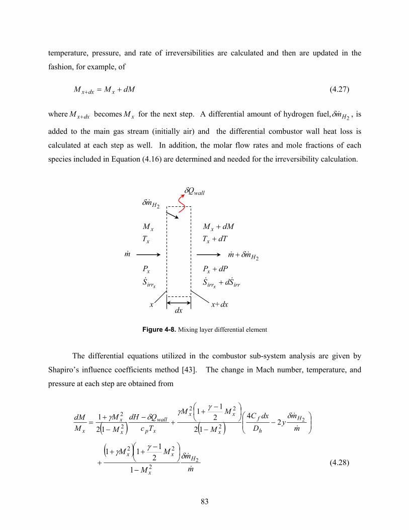
83

temperature, pressure, and rate of irreversibilities are calculated and then are updated in the

fashion, for example, of

dMMM xdxx +=+ (4.27)

where dxxM + becomes xM for the next step. A differential amount of hydrogen fuel, 2Hm&δ , is

added to the main gas stream (initially air) and the differential combustor wall heat loss is

calculated at each step as well. In addition, the molar flow rates and mole fractions of each

species included in Equation (4.16) are determined and needed for the irreversibility calculation.

Figure 4-8. Mixing layer differential element

The differential equations utilized in the combustor sub-system analysis are given by

Shapiro’s influence coefficients method [43]. The change in Mach number, temperature, and

pressure at each step are obtained from

( ) ( )

−

−

−+

+−

−

+=

mm

yD

dxC

M

MM

TcQdH

MM

MdM H

h

f

x

xx

xp

wall

x

x

x &

&22

4

122

11

121

2

22

2

2 δγγ

δγ

( )

mm

M

MMH

x

xx

&

&2

2

22

12

111 δγγ

−

−++

+ (4.28)

wallQδ

xirr

x

S

P&

m&

dx

2Hmm && δ+

x

x

TM

dTT

dMM

x

x

++

irrirr

x

SdS

dPP

x&& +

+

2Hm&δ

x x+dx

84

( )( )

−

−

−−

−

−

−=

mm

yD

dxC

MM

TcQdH

MM

TdT H

h

f

x

x

xp

wall

x

x

x &

&22

4

121

11

2

4

2

2 δγγδγ

( ) ( )

mm

MMM H

x

xx&

&2

2

22

111 δγγ

−

+−− (4.29)

( )[ ]

( )

−

−

−+−

−

−−=

mm

yD

dxC

MMM

TcQdH

MM

PdP H

h

f

x

xx

xp

wall

x

x

x &

&22

4

1211

1 2

22

2

2 δγγδγ

m

m

M

MMH

x

xx

&

&2

2

22

12

112 δγγ

−

−+

− (4.30)

where the hydraulic diameter of a rectangular duct per unit width, hD , and the hydrogen-to-main

stream axial velocity ratio, y, are defined as

1

2+

=x

xh A

AD (4.31)

throatx AA = (4.31a)

and x

x

u

uy H2= (4.32)

Note the dH and wallQδ are non-rate quantities with the former explained immediately below

and the latter in the section Combustor Wall Heat Loss Model. In addition, the first group of

terms on the right hand side of Equations (4-28) to (4-30) represents the influence of energy

addition from fuel and convective heat loss on the main stream Mach number, temperature, and

pressure. The second group of terms represents the influence of drag due to wall skin friction,

injectors45, and mass addition on the main stream Mach number, temperature, and pressure. The

final group of terms represents the affect of mass addition on the aforementioned properties.

A term common to Equations (4-28) to (4.30) is an energy term defined by

45 In the combustor model used in this analysis, the drag to injectors is directly incorporated into the skin friction coefficient for simplicity. Another term, however, can be included in the second group on the right hand side of Equations (4.28) to (4.30). See Shapiro [43] for more details.

85

( )m

muTTcdhdH Hx

txppr HH &

&2

22 2

2 δ

+−−= (4.33)

that includes enthalpy changes due to both chemical reaction and temperature difference between

the injection total temperature, 2HtT , and main stream mixture temperature, xT . The amount of

fuel absorbed into the mixing layer at each step and the amount of energy released each step are

predicted by mixing efficiency and combustion efficiency models, both of which are described

shortly.

The combustor component model implemented in this analysis requires two major

assumptions regarding the injection of the fuel. First, fuel mass addition (mixing) and

combustion are assumed to commence immediately downstream of the combustor entrance

interface, i.e. combustion ignition delay and injector position are ignored. Second, fuel is

assumed to be injected (absorbed) continuously along the combustor duct length and into the

mixing layer. Both of these approximations create a simplified model of a real injection process.

Mixing and Efficiency Models

As previously mentioned, the hydrogen fuel is injected into the combustor and then

incremental amounts are absorbed into the mixing layer as the flow proceeds from combustor

entrance to combustor exit. The mass flow rate of the unabsorbed hydrogen stream at any axial

combustor location is calculated in [1] as

( ) ( )( )xfmxm MstairH ηφ −= 152&& (4.34)

with knowledge of the mixing efficiency, Mη , the equivalence ratio φ , and the stoichiometric

fuel-to-air ratio, stf . With the mass flow rate of the unabsorbed hydrogen stream known at

stations x and x+dx, the amount of fuel absorbed into the mixing layer each step is given by

dxxx HHH mmm

+−=

222&&&δ (4.35)

Equation (4.34) reveals the need for a mixing efficiency to be defined as a function of axial

combustor length. A study of chemical kinetics in scramjet burners suggests an exponential

86

function representation for the mixing efficiency [55]. The mixing efficiency model used is

taken from [1] in this analysis and is defined as

( ) A

LAx

Me

exm

−

−

−

−=

11η (4.36)

where A is a fit parameter that represents near-field mixing and mL is the distance for minor

mixant to be mixed to stoichiometric proportion (depleted). The fit parameter A typically varies

in the range 1 to 5 and for this analysis it is chosen to be 5.4=A [56, 57]. If the equivalence

ratio is less than or equal to unity, the fuel is considered the minor mixant and if the equivalence

ratio is greater than unity, the air is considered the minor mixant. The axial distance at which the

minor mixant is depleted is given by the relations

φ72.1179.0 ebCL mm ≅ 1≤φ (4.37)

φ204.1333.3 −≅ ebCL mm 1>φ (4.38)

where throatAb = and the mixing constant is mC . The mixing constant is reported to vary from

values of 25 to 60 and is chosen to be 47=mC for this analysis [61]. It is evident from

Equation (4.36) that the mixing efficiency equals unity when combustor length equals the length

for the minor mixant to be depleted, i.e. 1=Mη when mcomb LL = . The exponential nature of

the mixing efficiency, along with the combustion efficiency (defined below), is illustrated in

Figure 4-9 for an example combustor length of 1 m (assumes 1=mL as well).

A combustion efficiency model is required to calculate the incremental energy release by

the fuel per step in Equation (4.33). As seen in Figure 4-9, the combustion efficiency is also an

exponential function, however, it grows at a slower rate than the mixing efficiency and attains a

value of 9.0=bη at a value of 1=Mη . The relations for the combustion efficiency model and

the incremental energy release at a given axial location are described by, respectively,

( ) mLBx

b ex−

−= 1η (4.39)

87

( ) ( ) prbprbpr hxhdxxdh ηη −+= (4.40)

The coefficient B is once again a fit parameter and is chosen to be 3.2=B to provide the

characteristics displayed in Figure 4-9.

0 0.1 0.2 0.3 0.4 0.5 0.6 0.7 0.8 0.9 10

0.1

0.2

0.3

0.4

0.5

0.6

0.7

0.8

0.9

1

Combustor Length (m)

Effi

cien

cy

MixingCombustion

Figure 4-9. Axial growth of the mixing and combustion efficiencies for the combustor component.

Combustor Wall Heat Loss Model

The total enthalpies encountered in the combustor during hypersonic flight demands the

need for combustor wall cooling to avoid material temperature limits. This is accomplished by

using the fuel to be injected into the combustor as the coolant and, thereby, preventing excessive

energy ‘waste’. Before the amount of fuel necessary for cooling can be calculated, an estimate

of the convective wall heat transfer must be provided.

The technique used in this thesis work to estimate the convective wall heat transfer is the

Eckert Reference Enthalpy Method [1]. This method is based upon the premise that the overall

effects of a variable property boundary layer can be replaced by those of a constant property

boundary layer whose properties reflect that of an average reference enthalpy and temperature.

A significant restriction on this method is that it cannot be applied when species dissociation

occurs.

The first step in the Eckert reference enthalpy method is to solve for the reference

enthalpy from

88

2

22.02

2* ewe u

rhh

h ++

= (4.41)

where the recovery factor r is determined from the relationship

2

2e

eaw

uhh

r−

= (4.42)

In Equations (4.41) and (4.42) the subscript e refers to the undisturbed flow at the outer edge of

the boundary layer at the combustor entrance, i.e. station 5 while w refers to the conditions at the

wall and aw refers to adiabatic wall. The adiabatic wall enthalpy and the enthalpy at the

combustor entrance need to be determined for calculation of the recovery factor and are done so

by knowledge of the total temperature and static temperature, respectively. The maximum

combustor wall temperature desired is set to KRTw 7.10881960 == o for this analysis. This

temperature (Tw) is used to obtain the wall enthalpy and is used in conjunction with the recovery

factor and station 5 properties to compute the reference enthalpy (Equation (4.41)). Iteration is

then utilized to obtain the reference temperature T* which is required to determine the convective

wall heat flux from the following:

( )

5152 *** RePr

0287.0

x

waweewall

RT

hhuPq

−=& (4.43)

***Re

µRTLuP combee

x = (4.44)

31*Pr r= (4.45)

The reference Prandtl number and the convective wall heat transfer relations, given by Equations

(4.44) and (4.45), respectively, assume turbulent flow at the combustor entrance. It is apparent

that the reference Prandtl number is simply a function of the recovery factor and the convective

wall heat transfer is a function of both reference and combustor entrance conditions. The units

of the heat flux wallq& in Equation (4.43) are 2mW . Therefore, to obtain the differential heat

89

loss per step ( )wallQδ on a per unit mass basis in Equations (4.28) to (4.30), Equation (4.43)

must be divided by the combustor entrance mass flow rate and then multiplied by the differential

surface area46 ( )12 += xsurf AdxdA . Additionally, the reference kinematic viscosity required for

calculation of the reference Reynolds number is given by the correlation [1]

( )111

1046.1 *

*6*

23

+= −

TTµ (4.46)

Although the Eckert Reference Enthalpy Method is based upon combustor entrance and

reference conditions, it provides a reasonable approximation to the convective wall heat loss.

Available experimental and analytical data support this statement and estimate that convective

heat transfer values based on the Eckert method are very likely to be within 10 to 20 percent of

the correct value [1].

With knowledge of the total heat removal rate and the hydrogen fuel injection

temperature, KTH 6002 = , the mass flow rate necessary to cool the combustor surfaces can be

determined. In this thesis, hydrogen is assumed to be stored in a liquid state and heated to a

vapor state, as a result of combustor heat absorption, before being injected into the combustor.

The relation

( ) ( ) ( )100400100400210022 tan −+−++−=

HHHliq pvappvapkvappfc cTchTTch

( )40026002−+ Hp Tc

H (4.47)

is used to calculate the amount of thermal energy that is absorbed by each unit mass of fuel in

going from storage conditions to injection conditions. Equation (4.47) is the sum of the enthalpy

of vaporization of hydrogen, kgkJhvap 3.454= , and all the sensible enthalpy increases over a

given temperature range. The specific heats used in Equation (4.47) are averaged over the

temperature range in the adjacent parenthesis. The vaporization temperature of liquid hydrogen

is known to be KTvap 35.20= . Therefore, the mass flow rate needed for cooling is determined

from

46 This is for a rectangular duct per unit width.

90

fc

wallH h

Qm

need

&&

5.12 = (4.48)

where wallQ& is the heat flux wallq& multiplied by the wall surface area and the factor of 1.5 is

added to the numerator to account for heat removal in the nozzle, i.e. nozzle heat loss is assumed

to be 50 percent47 of combustor the heat loss. Realistically, an iterative scheme between the

combustor and nozzle would be required to properly thermally balance the vehicle. However,

doing so for the work done in this thesis would potentially produce a computational burden in the

optimization process which would be unacceptable at this juncture48. If the needed mass flow

rate predicted by Equation (4.48) is greater than that determined from the equivalence ratio, the

extra mass flow of hydrogen is assumed to be re-circulated back to the storage tank.

Irreversibilities Due to Loss Mechanisms

There are four major loss mechanisms attributed to the combustor component in this

thesis. These loss mechanisms are friction, heat transfer across a finite temperature difference,

fuel/air mixing, and incomplete combustion49. Each individual loss mechanism creates an

irreversible increase in entropy, which is calculated at every differential step (dx). The relations

for the rate irreversibility increases due to friction, heat transfer, incomplete combustion, and

mixing are given respectively, as

xx

surfxfirr AT

dAuCmSd fric 2

2&& = (4.49)

−=

wHwallirr TT

QSdht

11

2

&& δ (4.50)

−=

xHprHirr TT

dhmSdcombinc

11

22

&& (4.51)

47 The value is assumed based upon individual component assessment. 48 In effect more computing power in the form, for example, of a distributed set of PC workstations would be required for the large-scale optimization used here. As is, only a single PC workstation was available for this work. 49 The unburned fuel taken into account with the combustion efficiency is a loss but not a loss mechanism which results in an increased entropy generation.

91

∑

+−−= +

j

x

dxxpjirr

x

prH

w

wallirr T

TcmSd

Tdhm

TQ

Sdjfricmix

1ln2 &&

&&& δ

−− ++

x

dxx

j

j

x

dxxx

xR

PP

R lnln (4.52)

where xj is the mass fraction calculated from

MWMWy

x jjj = (4.53)

using the mole fraction yj and the molecular weights of each constituent and the main gas stream

(MWj and MW, respectively). The rates of irreversibility increases predicted by Equations (4.49)

to (4.52) are all in units of KkW and are updated each step as shown in Equation (4.27). The

rate of irreversibility produced by heat transfer is calculated by drawing a control volume

containing the combustor walls only. Incomplete combustion losses are obtained by drawing a

control volume around the fuel stream and main stream (mixing layer) interface. The mixing

losses are determined from an entropy balance (Equation (3.8)) on a differential element of the

main stream. The sum of all these losses results in the total rate of irreversibility produced by

the combustor, i.e.

mixcombinchtfrictcomb irrirrirrirrirr SSSSS &&&&& +++= (4.54)

It is evident from Equation (4.52) that the mass flow rates and mass fractions of each constituent

( thj ) must be determined for prediction of mixing losses. Additionally, the molar flow rates of

each constituent entering the combustor must be computed for equations to follow and this is

done from knowledge of the corresponding mass flow rates and molecular weights. The mass

flow rate of hydrogen is known at both x via the mixing model and x + dx via the assumption that

all the hydrogen entering the mixing layer is consumed50. Therefore, the molar flow rates are

known as well and are used to calculate the reaction coordinate rate [24], i.e.

εν &&& +=inout HH nn

22 (4.55)

50 The reasonableness of this last assumption is discussed following Equation (4.59)

92

From the assumption of complete combustion, outHn

2& is zero and from the mixing model,

dxxxin HHH nnn

+−=

222&&& (4.55a)

Thus, from the reaction mechanism 1=ν for hydrogen and the reaction coordinate rate is

1

22

−

−= + xdxx HH nn &&

&ε (4.55b)

As a result, the remaining constituent molar flow rates and the mole fraction of each constituent

are given by

( )ε&&& 5.022

−+=+ xdxx OO nn (4.56)

xdxx NN nn

22&& =

+ (4.57)

ε&&& 122 +=+ xdxx OHOH nn (4.58)

∑= j

j

jj

n

ny

1&

& (4.59)

where once again the stoichiometric coefficients of oxygen and water are taken from Equation

(4.24). The combustor exit flow mole fractions are passed to the nozzle sub-system along with

the flow properties and necessary geometric parameters for nozzle evaluation.

Finally, an explanation is in order regarding the assumption of complete combustion used

to calculate the mole flow rates in Equations (4.55) to (4.58), i.e that all the hydrogen entering a

differential element is consumed. In terms, of equilibrium, it turns out that for the typical range

of temperatures (1000 K to 4000 K) and pressures (100,000 N/m2 – 600,000 N/m2) involved at

the combustor entrance, the deviation of equilibrium from complete combustion of H2 is about

4.5% at a maximum and usually much less than this (on the order of tenths of a percent of less)

towards the lower end up the above mentioned ranges of temperature and pressure. As to non-

equilibrium or kinetic considerations, the deviations from complete combustion depend of

course, on residence times which for the conditions see by the combustor are probably on the

93

order of 10-4 seconds. As can be seen from Figure 4.10 [1], the reaction rates for the species

involved are on the order of 10-5 seconds at 1500 K which leads to the reasonable assumption

that the kinetic results must also be fairly close to those for the complete combustion of H2. In

fact, at temperatures much close to the low end of our range (i.e. to 1000 K), the deviations can

be important but due to the goal of the modeling being done here, i.e. that of vehicle

optimization, they are not taken into account in the calculation of the reacted species mole flow

rates.

Where non-equilibrium effects are considered is in the use of the combustion efficiency

schedule given in Figure 4-9 and appearing in Equation (4.40) and in the calculation of the rate

of entropy generation for incomplete combustion, Equation (4.51).

Figure 4-10. Isobaric batch reaction of stoichiometric hydrogen and air mixture. Initial conditions are: P = 2 atm, T = 1500 K. From Heiser et al. [1]; reprinted by permission of the American Institute of Aeronautics and Astronautics.

94

4.1.3 Nozzle Component Description and Modeling51

The combustor exit conditions at station 6, equivalent to the nozzle entrance conditions,

are expanded to the nozzle component exit plane, labeled station ‘7’ (see Figure 4-11), to provide

the vehicle thrust. The nozzle sub-system is modeled with ‘frozen’ chemical kinetics, i.e.

recombination and dissociation of species exiting the combustor are ignored. The two loss

mechanisms incorporated into the nozzle sub-system are friction and heat transfer at a finite

temperature difference. A physical representation of the nozzle sub-system is displayed in

Figure 4-11.

Two design decision variables are assigned to the nozzle component. One of those is the

nozzle expansion angle, nozzθ , which, as shown in Figure 4-11, is simply the angle between the

vehicle aftbody and the combustor reference line. The other decision variable is the extcowl%

and is defined by

nozz

cowlextcowl L

Lnozz=% (4.60)

which is merely the ratio of the length that the cowl extends into the nozzle to the total nozzle

length. The length of the nozzle is fixed by the previously determined inlet and combustor

lengths and the overall vehicle length.

Only two constraints are imposed on the nozzle component for this analysis. The nozzle

expansion angle cannot be larger than o18 because undesirable, two-dimensional boundary layer

separation effects manifest beyond this limit [58, 60]. Also, the nozzle exit area referenced from

the cowl reference line (i.e. excluding plume area) must be less than 2.5 times the inlet capture

area. This constraint is aimed at preventing excessive nozzle exit areas and possibly

overexpansion.

The same differential ‘marching’ scheme as used in the combustor is employed in the

nozzle analysis, except with slight variations in the differential equations. The change in Mach

number, total pressure, and total temperature at each step are governed by

51 The nozzle component model presented here was developed as part of the M.S. thesis work [62] of K. M. Brewer at Virginia Tech who has worked in collaboration with me on the developing the hypersonic vehicle model. His work is ongoing with an anticipated completion date of May 2005.

95

+

++−

−

−+

=h

fxt

tx

xx

x

x DdxCM

TdTM

AdA

M

M

MdM

x

22

2

2

22

11

211

γγ

γ

(4.61)

+−=

h

f

t

tx

t

tD

dxCTdTM

PdP

xx

42

2γ (4.62)

xp

wall

xt

tTc

Q

MTdT

x

δγ

−

−+

=2

211

1 (4.63)

The skin friction coefficient in Equations (4.61) to (4.63) is held constant at 005.0=fC as

suggested by Riggins [58]. The specific heat ratio is calculated based upon the chemical

composition and properties of the combustor exit flow and is held constant at that value. The

specific heat is also determined from the chemical composition, however, it is adjusted each step

based upon the local temperature, xT . Also, in Equations (4.61) to (4.63), it is important to

include the additional area resulting from the exhaust plume when calculating area changes. On

a similar note, an appropriate hydraulic diameter must be specified as a function of nozzle

length, i.e. it changes when the cowl extension portion ends. The nozzle hydraulic diameter is

defined as

x

xh A

AD inner +

=12

(4.64)

for the portion of the nozzle which contains the cowl extension and as

xh AD outer 4= (4.65)

for the portion of the nozzle where the plume exists.

The nozzle component also makes use of the Eckert reference enthalpy method to predict

nozzle heat losses (see the combustor component) and maintains the same maximum wall

temperature as that used by the combustor. However, it has been determined that this method

96

over-predicts the heat loss by a rather substantial portion52. This is because, in reality, the heat

loss in a nozzle is greatest in the vicinity of the combustor exit and drops off considerably as the

flow is expanded to nozzle exit conditions. Therefore, to compensate for this decline in heat loss

a simple assumption is made based on Riggins [58] that the heat loss is half of that provided by

the Eckert Method. This is consistent with the assumption made in the combustor where the

nozzle heat loss is taken into account when determining the mass flow rate of fuel needed for the

vehicle surface cooling. Again, as mentioned earlier, this is to avoid a possibly significant

computational burden which would be imposed by iterating between the nozzle and combustor.

Figure 4-11. Nozzle component schematic including station numbers and other geometric parameters.

The shape of the exhaust plume as seen in Figure 4-11 is determined from the

combination of Newtonian and Modified Newtonian theories [63]. The location of the plume

‘line’ is where, at each step, the exhaust pressure xP equals the pressure outside the plume,

termed xouterP . The pressure outside the plume is given by

52 This statement has been substantiated in private discussions with Riggins [58] and through component investigations.

97

( )

+= plumecowlp

cowlcowlouter MC

MPP

comxθγ

γ,,

21

2 (4.66)

where the compressible pressure coefficient is defined for the Newtonian and Modified

Newtonian theories, respectively, as

( )plumepcomC θ2sin2= (4.67)

( ) ( )

( )( )

−

+−−

−−

+=

−1

112

1241sin2 21

2

22

2

2

γγγ

γγγ

γ

θ γγ

cowl

cowl

cowl

cowl

plumep

MM

MM

C com (4.68)

It is apparent that the pressure coefficient predicted by the Newtonian theory is a more general

approximation and is a function of the plume angle only. Also, in Equations (4.66) to (4.68) the

subscript cowl53 refers to the freestream conditions under the cowl and outside the plume.

Matching the inner and outer plume pressures can be a rather troublesome task. At large

ratios of cowlPPx (encountered in regions close to the combustor exit), the plume angle required

(as determined from Equations (4.66)-(4.68), to equate the inner and outer plume pressures

becomes larger (sometimes much larger) than o90 . This is deemed undesirable because it

inhibits the nozzle solution procedure significantly54. Therefore, to correct this difficulty, the

plume angle is fixed at o75 when the aforementioned pressure ratio is greater than the ratio that

would produce a plume angle greater than o75 . To determine these limiting pressure ratios over

various ranges of cowlM , Equation (4.66) is used in conjunction with Equation (4.67) for

o75=plumeθ . The Newtonian pressure coefficient is chosen because it is not a function of either

the specific heat ratio or cowlM . When cowlPPx is less than the limiting pressure ratio, an

iterative solution procedure is employed to find the plume angle which equates the inner and

outer plume pressures.

53 These conditions are not the same as that of station 0 because of the oblique shock under the cowl (see Figure 4-1). 54 In fact, it prohibits the convergence of the plume angle at values of about 90°.

98

The rate of irreversibility due to the nozzle loss mechanisms is calculated in a manner

different from the combustor. An entropy balance is applied over a control volume

encompassing the entire nozzle and is written as

w

wallj

jj

j

jjmixirr TQ

PP

RsysymSnozz

&&& +

−−= ∑∑

6

7

11log

67 (4.69)

where the mole fractions of each constituent remain constant throughout the nozzle and the

irreversibility is in units of KkW .

The nozzle component model, like that for the inlet component, calculates the vertical

surface forces which will be used by the airframe sub-system for lift prediction. Also, the

moment produced by the vertical surface forces is determined with knowledge of the vehicle

center of gravity. As a result of the high pressures exiting the combustor, the nozzle, without a

cowl extension, produces rather large force and moment values. Therefore, the design decision

variable extcowl% is included to allow a greater flexibility regarding the production of forces and

moments. This topic is also touched upon in the airframe sub-system discussion.

4.2 Airframe Sub-system Description and Modeling55

The airframe sub-system performs many tasks to determine whether the generated

vehicle configuration is acceptable for given flight conditions. One main function is to calculate

the external vehicle surface forces (i.e. non-propulsive forces) and determine the total pitching

moment as a result of these forces and the propulsive forces. The airframe sub-system must

provide a means to trim the pitching moments during all flight conditions. Another main

function of this sub-system is to estimate the lift needed from additional planform area, which for

this thesis work is a wing. Vehicle volume and weight estimations are also made, both of which

play an important role in predicting vehicle trim and wing size. Finally, the airframe sub-system

ensures that the thrust required to perform a specified mission is provided.

55 The airframe sub-system model presented here is the combined effort of the M.S. thesis work of K. M. Brewer at Virginia Tech and me. His work is at present on-going with an anticipated completion date of May 2005.

99

4.2.1 Vehicle Volume and Center of Gravity Estimation

The determination of the vehicle volume and center of gravity is essential to the

computation of pitching moments and vehicle weight. Vehicle volume is calculated by

integration of line segments to find the area under the curve and the center of gravity is estimated

by dividing the vehicle into a series of ‘panels’. A complete hypersonic vehicle sketch (side

view only) is provided in Figure 4-12 to supplement the discussion of vehicle volume calculation

and to show an example center of gravity position. Figure 4-13 displays the vehicle broken

down into ‘panels’ to provide a simple means of estimating the center of gravity.

Once the forebody and inlet geometry is established, the vehicle volume per unit width

can be calculated. As seen in Figure 4-12, six line segments are created, for example, 12 , 13 ,

etc.; and the equation for each line segment is determined. Each equation is then integrated over

its appropriate ‘x’ distance to find the area under the line segment. Knowledge of the six areas

permits the calculation of vehicle volume per unit width. The mathematical representation of the

volume per unit width (i.e. area) is given by

( ) ( ) ( ) ( ) ( )∫ ∫ ∫ ∫ ∫−−−−=∀2

1

3

1

4

3

5

4

2

6

6245341312

x

x

x

x

x

x

x

x

x

xveh dxxfdxxfdxxfdxxfdxxf (4.70)

where 12f , 34f , etc. are the equations of the lines.

Figure 4-12. Reference points for vehicle volume calculation.

The centroid of the vehicle is determined by a technique known as the method of

composite areas [64]. Since this analysis assumes a homogeneous distribution of vehicle weight

100

(fuel evenly distributed throughout body as well), the center of gravity ( )cgcg yx , coincides with

the centroid of the vehicle. Figure 4-13 displays the five panels (A, B, C, D, E) used in the

centroid calculation with each panel being either a triangle or a rectangle. The coordinates of the

vehicle center of gravity are defined as

i

iicg A

xAx ∑= (4.71a)

i

iicg A

yAy ∑= (4.71b)

where subscript i represents an individual panel and yx, define the location of each panels

centroid as shown in Figure 4-13 for panel A.

Figure 4-13. Five panels used to estimate the center of gravity. Each panel has its centroid marked by a bullet. The actual vehicle surface is displayed as light, small dashed lines.

4.2.2 Force Accounting and Moment Trim

The force accounting system utilized in this thesis is known as the ‘ramp-to-tail’ method

[21]. A method such as this is used to ensure that all forces are taken into account and no force

is ‘double-booked’ (i.e. counted more than once). There are various other force accounting

methods, each possessing their own strengths and weaknesses [49-52]. An airframe/propulsion

interface is developed to divide the pressure and shear forces acting on the vehicle surfaces into

those charged to propulsion and those charged to the airframe sub-system. Figure 4-14

AyE

D

C

BA

•

•

• • •

Ax

101

illustrates all the surface forces acting on the vehicle and shows the airframe surfaces in blue and

the propulsion surfaces in red.

As seen in Figure 4-14, the airframe surface forces include both pressure and friction

forces whereas the propulsive surface forces are from pressure only56. The aerodynamic forces

are broken down into x and y-components, depending on the local inclination angle, to predict

vehicle lift and drag. Only the y-components of the propulsion forces are needed for lift

prediction while the x-components (i.e. drag) are incorporated into the streamthrust difference

between propulsion sub-system entrance and exit, i.e. 17 FF − . Once all surface forces are

known, the lift, drag, and thrust of the vehicle can be determined from

( ) ( ) αα sincos ∑ ∑∑∑ +−+= xxyy fpfpveh FFFFL (4.72)

( ) ( ) αα cossin ∑ ∑∑ ∑ +++= xxyy fpfpveh FFFFD (4.73)

( ) αcos17 FFTveh −= (4.74)

where the subscript f represents friction, p pressure, and the forces are positive in the direction of

the reference axis in Figure 4-14. The minus sign is applied to Equation (4.72) because the sum

of all y-component forces act in the negative lift direction. However, the sum of all the x-

component forces act in the positive drag direction. The lift is calculated in the direction

perpendicular to the freestream flow and the drag is calculated in the direction parallel to the

freestream flow. The lift and drag directions are not the same as the x and y direction. This can

be seen in Figure 4-14 and, hence, the necessity for the cosine and sine terms in Equations (4.72)

to (4.74).

All the surface forces shown in Figure 4-14 are assumed to act at the center of the

appropriate surface segment. The interior cowl pressure force, occurring in both the inlet and the

nozzle, acts at the center of the cowl portion the projects into those components. The

streamthrust forces, 1F and 7F , are assumed to act at the midpoint of the inlet entrance area and

the nozzle exit area. The shear forces on the aerodynamic surfaces are determined from

56 The propulsion shear forces are a much smaller percentage of the total propulsion surface forces than compared to the airframe forces.

102

surff ACuF 221 ρτ = (4.75)

where local flow properties are used and are considered constant over the entire surface. Also,

the skin friction coefficient for the aerodynamic surfaces is fixed at 001.0=fC [58]. Finally,

the vehicle weight acts at the center of gravity computed by Equation (4.71) and the angle-of-

attack and vehicle flight angle are needed to compute the x and y-components of the weight

force.

Figure 4-14. Airframe and propulsive forces acting on the hypersonic vehicle.

The propulsion pressure forces are determined, as already noted, in the inlet and nozzle

components. The pressure and shear forces on the vehicle upper surface, forebody, and exterior

cowl surface are calculated in the airframe sub-system model. The forebody flow properties are

obtained in step 1 of the Inlet Solution Procedure section of the inlet component discussion.

With these flow properties and geometry known, the forebody pressure and friction forces are

easily obtained. The flow properties and forces underneath the cowl are obtained in a similar

fashion. However, the flow deflection angle is simply equal to the angle-of-attack. Finally, the

upper surface flow properties and forces are calculated with knowledge of the angle-of-attack as

well as the total capture area and nozzle exit area (measured from the cowl reference line).

These two areas permit the calculation of the upper surface deflection angle topθ from simply

103

geometry. Depending on the magnitudes of α and topθ , the flow either passes through an

oblique shock wave or an expansion wave. More specifically, if topθα > , the freestream flow

undergoes a Prandtl-Meyer expansion governed by Equations (3.23) to (3.26) and if topθα < ,

the freestream flow passes through an oblique shock wave governed by Equations (3.13) to

(3.20). Additionally, if an expansion occurs over the upper surface, then an oblique shock

emanates from the vehicle tail to return the flow to its original direction.

The moments resulting from the x and y-components of each force are determined with

knowledge of the forces location of action and the center of gravity. Clockwise moments are

considered positive and counter-clockwise moments are negative. The moment from the

forebody pressure force, for example, and the total pitch moment are given by

( ) ( )fbcgfbcgfbfbfb xxFyyFMypxpp −+−= (4.76)

∑ ∑+=fp FFpitch MMM (4.77)

where the total pitch moment must be trimmed (i.e. balanced) to provide stable flight. The pitch

moment is balanced in this thesis work by an elevon placed near the rear of the vehicle

(discussed in the next section). Note that the vehicle weight does not add to the pitch moment

because it is assumed to act at the vehicle’s center of gravity. Also, the nozzle moment (and

force) is calculated in the nozzle component at each differential step because of the large

variation of pressure over the nozzle surfaces, i.e. a more accurate moment calculation is

acquired.

The rate of irreversibility produced by the airframe sub-system result from oblique

shocks and aerodynamic drag. It is assumed in this analysis that the pressure drag (known as

wave drag) is reversible while the viscous dissipation resulting from friction produces the drag

irreversibility. The entropy generated by friction drag, given in Equation (4.78), is simply a

function of the friction force and the local temperature and velocity [65]. Equation (4.79)

provides the total irreversibility generated by airframe sub-system.

T

uFS f

irrfric =& (4.78)

104

∑ ∑+= shocksfricaero irrirrirr SSS &&& (4.79)

The shock irreversibility is that produced by the forebody oblique shock, exterior cowl oblique

shock, upper surface oblique shock, and the tail oblique shock. In calculating this value, the

same mass flow rate as that captured by the propulsion sub-system is used. The units of

Equation (4.79) are once again KkW .

4.2.3 Wing and Elevon Details

To approximate the additional lifting surface required and the trim balance moment,

fairly simplified wing and elevon models were developed. A wing, assumed to be independent

of the vehicle body, is incorporated as the additional lifting surface in this thesis work because it

provides a straightforward means for approximating the lift and drag coefficients. In reality, the

additional lifting surface may be a blended extension of the vehicle body outboard of the

propulsion sub-system (see Chapter 1) and therefore not a true wing. A plan view of the wing

and elevon concepts used in this analysis is given in Figure 4-15.

Figure 4-15. Plan view of vehicle showing wing and elevon concepts.

The wing and elevon are assumed to be of a simple delta configuration with a 5%

thickness-to-chord ratio (t/c) diamond airfoil cross-section [66, 67]. The wing is attached to the

vehicle body at a zero degree inclination angle and is assumed to be positioned such that its

105

center of pressure is in line with the vehicle center of gravity and, therefore, does not contribute

to the vehicle pitching moment. The elevon’s center of pressure is assumed to be located two

meters from the tail of the vehicle to be able, if necessary, to provide rather large trim balance

moments. The diamond airfoils are assumed to be inviscid and, therefore, shock-expansion

theory57 is implemented in the calculation of the lift and drag coefficients. A schematic of the

diamond airfoil cross-section is given in Figure 4-16 at some fixed angle-of-attack which, along

with the freestream flight conditions, allows the pressure distribution shown in the figure to be

calculated.

Figure 4-16. Diamond airfoil cross-section used to describe the wing and elevon. A given angle-of-attack and freestream properties produce a pressure distribution as shown. The airfoil thickness and chord length are shown as well.

The freestream flow is initially deflected into itself by an angle εα + on the bottom

surface of the airfoil, thereby passing through an oblique shock wave. The Mach number and

pressure downstream of the shock (c) are obtained from the oblique shock relations provided in

Chapter 3. The flow is then expanded through an angle ε2 where the Prandl-Meyer expansion

relations are used to determine the Mach number and pressure at location d. The flow is then

either shocked or expanded back to its original direction, depending on the magnitude of the

angle-of-attack. The freestream flow can be either initially compressed or expanded on the top

surface (a), once again depending on the magnitude of the angle-of-attack. If compressed, the

57 Shock-expansion theory exactly predicts the lift and drag coefficients of inviscid diamond airfoils [3].

106

flow deflection angle, as seen in Figure 4-16, is equal to the quantity αε − and otherwise, the

flow expands through the angle εα − . Like the bottom surface, the flow then expands through

an angle ε2 to conditions at b and then shocked back to the freestream flow direction. Also like

the bottom surface, oblique shock and Prandtl-Meyer relations are used to determine the Mach

number and pressure at both a and b.

Once the pressures at a, b, c, and d are determined, the lift and drag per unit span can be

calculated and used to determine the lift and drag coefficients for the diamond airfoil. For the

condition εα > , the lift and drag coefficients are given as

( ) ( )

−

−++

−= εαεαγ

coscos2

0020 P

PPP

PPcM

lC adbcL (4.80)

( ) ( )

−

−++

−= εαεαγ

sinsin2

0020 P

PPP

PPcM

lC adbcD (4.81)

where the chord length c, represented by the dashed line in Figure 4-16, is determined from

trigonometric relations and is written as

( )( ) 212cos12 επ −−= lc (4.82)

Equations (4.80) to (4.82) are developed using the assumption that the maximum airfoil

thickness occurs at 50% of the chord length. The term l is the length of each of the four surfaces

of the diamond airfoil. Equations (4.80) and (4.82) are almost identical for the condition αε >

with some subtle differences in signs.

Instead of using the flight angle-of-attack for calculation of the lift and drag coefficients,

the elevon iterates through a range of positive and negative deflection angles (relative to the

freestream) to see if the pitch moment determined by Equation (4.77) can be trimmed. An

elevon area needs to be specified to calculate the lift and drag of the elevon, which for this thesis

work is given by Equation (4.83) where the control volume requirement 04.0=elevV [36].

−

=

veh

cg

vehelevelev

LxLV

S1

(4.83)

107

The calculated lift and drag of the elevon is not in the same direction as the lift and drag of the

vehicle and, therefore, it must be resolved into the appropriate direction. The elevon deflection

angle is given by the symbol ω .

For all flight conditions considered in this thesis work, the total lift must equal the

instantaneous weight of the vehicle, i.e. vehtotal WL = 58. The total lift is the sum of the lift

provided by the vehicle body and that provided by the wing and elevon. After calculation of the

vehicle lift from Equation (4.72) and the lift of the elevon at the required deflection angle, the lift

needed from the wing is

elevvehtotalwing LLLL −−= (4.84)

which can then by used with the dynamic pressure and lift coefficient to determine the wing

planform area wingS . Finally, the total drag is given by

elevwingvehtotal DDDD ++= (4.85)

which is, once again, in the direction parallel to the freestream velocity. Equation (3.3) is used to

obtain the drag of the wing and elevon.

4.2.4 Mass Fractions and Weight Estimation

A simplified approach is applied in this thesis work to estimate the empty mass of the

vehicle, the amount of fuel needed for each mission segment, and consequently the overall

vehicle weight. This is necessary because of the lack of analytical relations available for

hypersonic vehicle weight estimation which is unlike the case for subsonic or supersonic aircraft.

The empty mass of the vehicle is determined from an investigation of potential hypersonic

vehicle designs presented in [21] and also in [36, 41, 42]. The empty mass of the vehicle is

chosen to be kgme 5000= per unit width for this work, and it is assigned to a vehicle area59 (i.e.

volume per unit width) of 225 m .

58 This statement is true for level flight. If the vehicle is at some angle of attack or climb angle, the weight must be resolved into the lift and drag directions. The resolved lift component of weight must then equal the total lift. 59 This area was determined through an evaluation of different vehicle configurations and was deemed an appropriated average value of the area.

108

In order to determine the overall vehicle weight at the beginning of the total mission, an

estimate must be made of the fuel consumed during each individual mission segment. The

fraction of the initial aircraft mass that must be fuel in order to accomplish a given mission

segment is known as the fuel mass fraction and is defined as [1]

i

final

i

finalif m

mmmm

−=−

= 1π (4.86)

The ratio ifinal mm is derived for a hypersonic cruise aircraft and a transatmospheric vehicle in

[1]. However, the equation presented for the transatmospheric vehicle is not in terms of desired

quantities and, therefore, is re-derived to reflect the equation given for the hypersonic cruise

aircraft. The fraction of the initial mass remaining at the end of a mission segment for a cruise

vehicle and a vehicle that climbs and accelerates are given respectively, as

−=

D

Lpro

i

final

CCh

Rgm

m

η

0exp (4.87)

( )

−++

−

−=pro

ifinalL

Difinal

i

final

h

zzRCCg

uu

mm

η

22exp

22

(4.88)

where 0η is the overall efficiency (see Equation (6.5)), g0 is the acceleration of gravity, and the

initial and final velocity and elevation as well as the range R are obtained from the definition of

the mission segment. However, Equations (4.87) and (4.88) require an estimation of the vehicle

lift-to-drag ratio and the overall vehicle efficiency oη . It is apparent that as engine overall

efficiency and lift-to-drag ratio increase, the fuel mass fraction decreases and as range increases

the fuel mass fraction increases. Once all the fuel mass fractions are obtained for the desired

mission segments, the initial mass (mass at the beginning of the mission) of the vehicle is

estimated by

109

( )∑−=

f

ei

mm

π1 (4.89)

which is simply the combination of the empty mass and the fuel mass. Obviously, if the initial

mass fraction does not match what is determined at the end of the mission, the mission must be

flown again to close the loop.

4.2.5 Airframe Sub-system Constants and Constraints

Like the propulsion sub-systems, the airframe sub-system uses constant values of the

specific heat ratio and constant pressure specific heat which are fixed at 4.1=γ and

KkgJc p ⋅= 1009 . Also, as previously mentioned, the skin friction coefficient on the vehicle

(not wing or elevon) surfaces is held at 001.0=fC . Finally, the vehicle is assumed to fly at a

fairly high constant dynamic pressure trajectory of 20 000,85 mNq = for the reasons mentioned

in Section 3.1 and the vehicle length is set to mLveh 24= .

One of the main airframe constraints is placed on the minimum and maximum allowable

wing planform area. For this work, the vehicle body width is assumed to be 4 m, therefore, the

total vehicle volume is 396 m . The minimum planform area is zero (no wing) and the maximum

planform area must be less or equal to 10% of the total volume60, i.e 22 6.90 mSm wing ≤≤ .

Since the wing area is calculated from the required wing lift at all mission segments (i.e. wingS is

an operational decision variable), the constraint vehtotal WL = is guaranteed at all flight

conditions.

Another constraint that must be included is the limit on the maximum elevon deflection

angle. This is necessary because as ∞→0M or 00 →P , the turning angle predicted by

Equation (3.23) approaches a finite value of o4.130 [48]. For example, following steps 1 and 2

of Section 3.2.3, an 71 =M gives ( ) o911 =Mν and, therefore, permits only a maximum elevon

60 The maximum constraint on the wing planform area was set to prevent unrealistically large planform areas when considering the entire three-dimensional vehicle. For example, if a wing planform area of 10% the total volume is needed to provide the remaining vehicle lift on a per unit width basis, then on a three-dimensional basis all the vehicle forces are 4 times as large (including vehicle weight) and consequently 4 times the wing planform area is needed to provide the remaining lift (i.e. 40% of the total volume).

110

deflection angle of o4.39=ω . As the freestream Mach number increases, the maximum elevon

deflection angle decreases. Thus, constraints are placed on the maximum elevon deflection

angle as a function of the freestream Mach number to avoid the breakdown of the Prandlt-Meyer

relations given in Equations (3.23) and (3.24).

A final constraint is placed on the amount of thrust produced by the vehicle. For cruise

missions, the vehicle thrust must equal the total vehicle drag, i.e. totalveh DT = . For acceleration

and climb missions, the vehicle thrust must equal that calculated from Equation (3.1). To

balance the thrust and drag or to obtain the desired thrust, iteration of the equivalence ratio

(adjusts amount of fuel injected into the combustor) is required. Each time the equivalence ratio

is changed a new pitching moment, wing area, and total drag is determined where they must all

satisfy individual constraints. As one can imagine, it can be quite difficult (if not impossible) or

time consuming to exactly balance the thrust and drag or obtain the desired thrust. Therefore,

this work uses a simplified approach to solving this problem. An initial equivalence ratio is set

to allow the calculation of the vehicle thrust and total drag. If totalveh DT > , the equivalence ratio

is decreased by increments of 1.0=φ until vehtotal TD > , then the equivalence ratio is increased

by increments of 02.0=φ until once again totalveh DT > . At this point the thrust and drag are

considered balanced. If initially the vehtotal TD > , the equivalence ratio is first increased and

then decreased in the same manner. The same approach applies in determining the necessary

thrust for acceleration and climb except now comparisons are made between the vehicle thrust

and the thrust predicted by Equation (3.1). This process is referred to as the throttling of the

thrust and in doing so, the equivalence ratio is limited to the range 0.20 ≤≤ φ with the upper

limit due to the hydrogen self-ignition criterion [54].

111

Chapter 5

Synthesis/Design Optimization Problem Definition and Strategy

In order to make strides towards achieving the thesis objectives set forth in Chapter 1, it

is quite evident that individual component analyses and single point optimizations (i.e. at a fixed

Mach number) will be required. However, to further demonstrate the utility of exergy methods

for determining hypersonic vehicle configurations, a complete hypersonic mission should be

specified. Therefore, this chapter presents the overall syntheis/design task at hand and discusses

the optimization approach that was implemented to achieve this design task.

5.1 Problem Definition

The synthesis/design optimization problem proposed here the integrated synthesis/design

optimization of the two sub-systems presented in Chapter 4 and their associated components, all

of which are part of a hypersonic airbreathing vehicle concept. The airframe and propulsion sub-

systems are the only two sub-systems considered, as opposed to the several optimized by

Rancruel [26] and Rancruel and von Spakovsky [27-29], because there is currently insufficient

information in the literature in regards to the other sub-systems that will be incorporated into

hypersonic airbreathing vehicles. Nonetheless, these are the two main sub-systems of a

hypersonic vehicle, providing the necessary lift and thrust to carry out a desired mission; and,

therefore, they are sufficient for performing preliminary analyses and optimizations as well as

demonstrating theory.

The mission is the set of conditions under which the hypersonic vehicle must be

synthesized/designed. The mission was developed in joint collaboration with Dr. D. Moorhouse

[68] at the Air Force Research Lab (AFRL) at Wright Patterson Air Force Base in order to

112

demonstrate the ability of the hypersonic vehicle to perform cruise and accelerations over a

rather large range of Mach numbers. It is emphasized that this is a purely arbitrary, empirical

mission defined to exercise the methodology of this thesis work. A general description of the

overall mission is displayed in Figure 5-1 along with a more detailed description in Table 5-1.

The mission has a total of 7 different mission segments consisting of a combination of cruises,

climbs, accelerations/decelerations as well as a turn. Only the hypersonic spectrum of flight is

considered in this mission; modeling of the hypersonic vehicle at subsonic, supersonic, and

transition from supersonic to hypersonic is not considered. To do so would require modeling of

a dual-mode scramjet engine as well as many other complexities and considerations associated

with hypersonic vehicles at these flight regimes.

Figure 5-1. Mission profile by segment.

As seen in Figure 5-1 and Table 5-1, the high speed climb to Mach 8 begins at Mach 6

for this work and is considered the lower limit of hypersonic flight. For all climb and

acceleration (or descend and decelerate) mission segments, the flight Mach number

(consequently the freestream flight properties) is taken to be the average of the initial and final

Mach numbers for that segment. The elevation range shown in Figure 5-1 corresponds to that

determined by the constant dynamic pressure trajectory of 20 000,85 mNq = throughout the

mission.

Payload Operation

Hypersonic

High Speed Climb to Mach 8

Mach 6 Cruise

Subsonic/Supersonic

Descend & Deceleration

23 km

30 km Mach 10 Cruise Acceleration Mach 8-10

Mach 8 Cruise

5000 nm

180º Turn

113

Table 5-1. Mission specifications.

Segment Description

1 Accelerate and climb from Mach 6 to Mach 8, t ≤ 90 s

2 Mach 8 cruise for 1500 nm



5 Perform a 180º, 2g sustained turn at Mach 10

6 Descend and decelerate to Mach 6 flight conditions


Before attempting to optimize a hypersonic vehicle over the complete mission described

in Figure 5-1 and Table 5-1, single flight Mach number optimizations for cruise and accelerating

vehicles will be performed to ensure the component models described in Chapter 4 are

functioning properly. Additionally, a partial mission comprised of three mission segments will

be optimized before the entire mission61 to make certain a solution can be found, primarily

because of the high non-linearity between sub-systems and strict constraints required by the

vehicle. This partial mission will also be useful to ensure that all the necessary parameters are

passed from mission segment to mission segment, to give some idea of the time required for

optimization, and ultimately to debug and correct any problems encountered in the models or

optimization process. Finally, this partial mission will be able to demonstrate the applicability of

exergy measures in hypersonic vehicle configuration optimization.

5.2 Optimization Technique

Prior to the optimization of any type of system, complete engineering system models

must be developed which typically begins with the selection of a number of degrees of freedom

(decision variables) represented by parameters which will be varied within acceptable limits

during the optimization process. These independent decision variables, hereby represented by a

vector xr , are then used to create two systems of equations to represent the model of the system,

i.e. 61 Note that only the individual mission segments and the partial mission comprised of three mission segments are used in this thesis work. The entire mission will be utilized in the thesis work of K. M. Brewer [62] scheduled for completion in May 2005.

114

( )( )( )

( )

03

2

1

=

=

xh

xh

xh

xh

H

nvvM

vv

vv

vv

v and

( )( )( )

( )

03

2

1

≤

=

xg

xgxgxg

G

nvv

M

vv

vv

vv

v (5.1)

The vector of equality constraints Hv

is composed of sub-vectors ihv

each of which

mathematically describes a phenomenon or set of phenomena (e.g., those in the inlet or

combustor) usually within the realm of a particular discipline. The elements of the sub-vectors

ihr

are known as the state equations. The vector of inequality constraints Gr

represents natural or

artificial limitations imposed upon the system. [26]

With engineering system and sub-system models in hand, optimization subject to a

desired set of constraints can now be performed. The system and sub-system models describe

the set of nonlinear constraints implemented in the formulation of the optimization problem. The

optimization problem is generally expressed as

Minimize or Maximize a function ( )xf v (5.2)

with respect to xv and subject to the following equality and inequality constraints:

( ) 0=xH vv (5.3)

( ) 0≤xG vv (5.4)

All equality constraints are active by definition whereas an inequality constraint 0≤jg is active

if 0=jg . The function ( )xf r is called the objective function. Three different objective

functions are used for vehicle synthesis/design optimization in this thesis work, namely, the

overall efficiency (Equation (6.5)) which is based on 1st Law considerations only, the rate of

exergy destruction (Equation (6.3)), and the rate of exergy destruction plus the rate of exergy

fuel loss (Equation (6.6)).

As a whole, the hypersonic vehicle system described in this thesis work can be viewed as

an energy conversion system. Unfortunately, energy conversion system models have a number

115

of characteristics which make them difficult to optimize. A few reasons for these difficulties are

presented by Leyland and are given as follows [69]:

1. Energy conversion system models are highly non-linear and, therefore, relatively robust

optimization tools must be used to optimize them.

2. Energy conversion system models often have a number of integer variables and even

combinatorial62 ones which cause the model to become discontinous and disjoint.

Therefore, the optimal surface does not have smooth derivates (the optimal surface has

jumps in it) and there are several completely different feasible regions, each having its own

“global” optimum and with no easy route for passing from one region to another.

3. From the viewpoint of an optimization algorithm, energy conversion system models must

often be treated as ‘black boxes’ – a set of parameters are presented as inputs and the black

box provides a number of outputs. Thus, derivatives of the outputs with respect to the

inputs and any extra information about the form of the model are usually not available.

If standard nonlinear programming techniques such as gradient-based methods (which are based

on assumptions of continuity in the optimal surface) are used to optimize such systems, they will

be insufficient and in most cases find a relative optimum closest to the starting point (i.e. a local

optimum).

To combat the aforementioned problems, a number of methods have been developed by

means of specialized search schemes. These types of algorithms specialize in performing a

complete search of the entire synthesis/design space and as a consequence are referred to as

global search algorithms [26]. One of the most popular and most developed methods for global

searches are Evolutionary Algorithms (EAs), also referred to as Genetic Algorithms (GAs).

An Evolutionary Algorithm is implemented in this work as the means of optimization.

The remainder of this section briefly discusses EAs, then describes the specific EA used in this

work, and finally a simple test problem is presented to demonstrate the EAs operation.

5.2.1 Evolutionary Algorithms (EAs)

Evolutionary Algorithms are based on the principles of genetics and Darwin’s theory of

natural selection. The basic elements of natural genetics – crossover, mutation, and selection – 62 For example, choosing which members of a set of possible components should be used.

116

are used in the genetic search procedure. The EA begins with an initial set of solutions, referred

to as the population, and the solutions from that population are used along with the

aforementioned operations to create a new population that will hopefully be ‘better’ than the old

population. This process is continuously repeated with the ultimate goal of obtaining the global

optimum.

Leyland [68] provides a brief discussion of the terminology used in EAs which

essentially describes how they operate. A population of individuals (possible solutions to the

problem) is evolved toward the solution of an optimization problem by means of operations

(mentioned above) on the population which produce new individuals and also by removing

unpromising individuals from the population. The population evolves toward a better solution

essentially by how the operators act on the population and how the individuals are removed from

the population. As previously noted, crossover and mutation are two natural genetic processes.

Crossover involves selecting two (or more) individuals from a population and creating a child (or

children) that is some way resembles it parents (selected individuals). The parents can be chosen

from the better parts of the population to ensure the children reflect the best of the current

population. The ‘better’ parts of the population are determined from the fitness of an individual,

i.e. the more suitable they are the better chances they have of reproducing. The fitness can often

be a direct reflection of an individuals objective function value. Diversity – the spread of a

population in the search space- is a characteristic of the population which assures that the

algorithm does not converge too quickly and get trapped in a local (non-global) optimum.

Generational, elitist, and steady-state EAs are three ways an individual can be removed

from a population. The population is processed a generation at a time in generational EAs, i.e. a

number of children equal to the size of the population is generated and completely replace the

existing population. In elitist EAs, the generation structure is generally retained, however, a few

of the very best individuals in the population are also retained from generation to generation.

Finally, steady-state EAs remove the generation structure of the algorithm and individuals are

added to and removed from the population as necessary; often based upon some form of elitism.

In general, properly conditioned EAs are robust optimizers that will solve most classes of

problems and, if given enough time, will find a good solution to almost any problem.

Additionally, EAs require no supplementary knowledge of the solution space (i.e. derivatives)

and require no initial ‘guess’ of the decision variables, whereas gradient-based methods do

117

require knowledge of derivatives and a ‘baseline’ set of decision variables values. Since EAs

work with a population of potential solutions, a single optimization run can return a range of

solutions, illustrating either a range of separate choices in a multi-modal problem or illustrating a

trade-off between objectives in a multi-objective problem [69]. One drawback to EAs is that

they tend to be computationally expensive (i.e. require long convergence times) and an

optimization problem, if it is not difficult to solve, can be solved quicker by gradient-based

methods; provided, of course, that it can solve it at all which oftentimes is not the case. Another

possible drawback to EAs is that multiple runs of the same optimization problem will often result

in different solutions to the problem due to the random nature of the search process. This,

however, can be overcome to a large extent by coupling the EA to a gradient-based method

which takes the solution developed by the EA and converges it towards the “global” solution.

This is the approach which was used in Munoz and von Spakovsky [32] and in Rancruel and von

Spakovsky [27, 28] with great success. Unfortunately, due to software integration and license

issues, it was not possible to couple the two types of optimization algorithms in this thesis work.

5.2.2 MooLENI Evolutionary Algorithm

The optimization tool implemented in this work is MooLENI, or more specifically, the

queueing multi-objective optimizer (QMOO). QMOO is an EA developed by Geoff Leyland and

Adam Molyneaux at the Laboratoire d’Energetique Industrielle (Laboratory of Industrial Energy

Systems, LENI) at the Ecole Polytechnique Federale de Lausanne (EPFL). QMOO was

developed at LENI for the optimization of energy conversion system problems.

QMOO is a steady-state EA; individuals are added to the population when they are ready

and are removed from the population when they are found lacking. QMOO is extremely elitist –

it has a single population that contains only the best individuals found thus far. Therefore,

QMOO converges rapidly but has trouble preserving diversity. To preserve diversity, QMOO

divides the population into groups in parameter space and then allows these groups to evolve

somewhat independently. QMOO also uses cluster analysis techniques to identify separate local

optima simultaneously and to also give it a higher chance of finding the global optimum.

Additionally, QMOO uses an algorithm flexible queue-based structure which makes it easy to

parallelize. Finally, QMOO is a rapid and robust optimizer that requires little tuning to the

specific problem at hand.

118

To obtain a more detailed description of the QMOO algorithm, acquire more information

of evolutionary algorithms, or to see various applications of QMOO, the reader is referred to the

doctoral dissertation of Geoff Leyland [69].

5.2.3 QMOO Test Problem

To demonstrate the operation of QMOO, a rather simple test problem is conducted using

a rather complex objective function. The test problem used here is known as the Woods function

and is considered an appropriate function when testing, for example, the robustness and speed of

algorithms of this nature. The optimization problem is defined as follows:

Minimize ( ) ( ) ( ) ( ) ( )2322

342

122

12 1901100 xxxxxxxf −+−+−+−=v

( ) ( )[ ] ( )( )118.19111.10 422

42

2 −−+−+− xxxx (5.5)

where 50,,,50 4321 ≤≤− xxxx (5.6)

It is apparent from a quick examination of the Woods function that the minimum value of ( )xf v

is 0 when 4321 xxxx === . QMOO was executed three times for the Woods test problem and

was discontinued when the objective function value became less than ( ) 510−=xf v . The results

of the three optimizations are given in Table 5-2 and a contour plot of the Woods function is

given in Figure 5-2 to display the optimal region. QMOO performed quite well in optimizing the

Woods function: however, it did require a varying amount of function evaluations to arrive

below the above limit. The optimizations took approximately 30 seconds to 1 minute on a 2.79

GHz Pentium 4 processor with 512 MB of RAM.

Table 5-2. Woods function optimization results.

Run Evaluations ( )xf 1x 2x 3x 4x

1 15,000 4E-6 1.0004 1.0008 0.9995 0.9992

2 11,700 8E-6 0.9999 0.9997 1.0000 1.0003

3 3,500 8E-6 1.0002 1.0003 1.0002 1.0003

119

Figure 5-2. Woods function contour plot with x3 = x4 = 1.

5.3 Design Problem Simulation and Coupling to EA

The mathematical models (component models) for this work are coded using MATLAB

software and make extensive use of function m-files in the programming. The optimization

software MooLENI is also coded in MATLAB. A single simulation of the hypersonic vehicle

model on a 2.79 GHz Pentium 4 processor with 512 MB of RAM requires anywhere from 10 to

30 seconds to complete depending on whether an accelerator or cruise vehicle is being throttled.

The hypersonic vehicle model and QMOO are coupled such that the optimizer generates

values of the decision variables and then passes them to the vehicle model where, if all

constraints are satisfied, an objective function value is calculated and passed back to the

optimizer63. If a constraint is violated anywhere throughout the hypersonic vehicle model, the

objective function is set to an extreme value so that the optimizer recognizes that the

combination of decision variables is undesirable. The 7 design decision variables implemented

in this work are cowlnozzfbcombrampcowlfb andLXXX %,,,,,, 1 θθ and the 2 operational decision

variables which vary from one mission segment to another are wingSandα (refer to the

component models for descriptions). The limits placed upon the design and operational decision 63 Note that the objective function is the only value passed to the optimizer, i.e. the optimizer has knowledge of only the decision variable values and the corresponding objective function values.

A - 10 B - 110 C - 210 D - 310 E - 410 F - 510 G - 610 H - 710 I - 810 J - 910

120

variables during the optimizations conducted in this thesis work are presented in Tables 5-3 and

5-4.

Table 5-3. Design decision variables and limits.

Decision Variables Imposed Limits

fbX vehfbveh LXL 65.035.0 ≤≤

cowlX vehcowlveh LXL 77.045.0 ≤≤

1rampX vehrampveh LXL 33.002.0 1 ≤≤

combL vehcombveh LLL 33.002.0 ≤≤

fbθ oo 61 ≤≤ fbθ

nozzθ oo 188 ≤≤ nozzθ

cowl% 25.0%0 ≤≤ cowl

Table 5-4. Operational decision variables and limits.

Operational Variables Imposed Limits

α oo 51.0 ≤≤ α

wingS 6.90 ≤≤ wingS

The wing planform area is allowed to vary over the mission (from one segment to

another) because initial optimization runs with a fixed planform area (determined from the first

mission segment) resulted in no solutions even after 1 million function evaluations. The need for

the wing planform area as an operational variable is most likely attributed to: (a) a hypersonic

vehicle may need a morphing wing structure to successfully fly a mission or (b) more exact

methods are required to predict surface forces (i.e. lift and drag).

121

Chapter 6

Results and Discussion

This chapter first presents the results of a preliminary analysis using exergy methods for

optimal combustor length prediction. Next a number of individual hypersonic vehicle

component investigations were conducted to gain insights into the hypersonic vehicle and its

relation to exergy destruction. The results of those investigations are presented and discussed

following the preliminary analysis. This is followed by the presentation of the propulsion sub-

system optimization results which are given along with a fixed geometry propulsion sub-system

analysis in order to investigate the trends of the propulsion system operating at different flight

Mach numbers. Finally, individual mission segment optimizations as well as partial mission (a

three segment mission) optimizations are presented and discussed, specifically looking at the use

of exergy measures in the optimization of hypersonic vehicle configurations.

6.1 Preliminary Analysis Using Exergy Methods

As a first investigation into the usefulness of exergy methods for hypersonic vehicle

synthesis/design, the simple design problem proposed by Riggins [9, 12] and previously

discussed in Section 2.2.1 is examined. The objective of this problem is to determine the optimal

combustor length of a scramjet engine which provides the best performance (i.e. thrust). The

simple scramjet engine along with some parameter values used in this problem are shown Figure

6-1. The scramjet engine is comprised of an isentropic inlet and nozzle (both of the same area

ratios) and a constant cross-sectional area combustor where Rayleigh heat addition takes place

and there is relatively high skin friction. The heat released into the flow is some fraction of the

total energy expended ( endexpQ∆ ) determined from an exponential combustion efficiency

schedule (a function of combustor length). An optimal combustor length can be determined

122

because there is some point in which the additional heat release associated with additional

combustor length is negated by the friction associated with that additional combustor length.

Figure 6-1. Optimal combustor length design problem

In the work done by Riggins [9, 12], a rational exergy efficiency based on earlier work by

Curran and Murthy [23] and a thrust-potential based engine effectiveness were both used to

predict the optimal combustor length to the above problem. It was shown that the rational

exergy efficiency significantly over-predicted the optimal combustor length64 and produced

much less thrust. In this investigation, the optimal combustor length predicted by the engine

effectiveness was compared to the optimal combustor length predicted by the thermodynamic

effectiveness which is based upon both the 1st and 2nd Laws of thermodynamics. The thrust-

potential-based engine effectiveness ( )xeeη and the thermodynamic efficiency ( )xε are defined

respectively, as

( ) ( ) ( ) ( )( )000

000APumAPumAPumAxPxum

xeee

eeeee

idealideal +−++−+

=&&

&&η (6.1)

64 As noted in Chapter 2, the rational efficiency proposed by Curran and Murthy [23] is more appropriate for stationary engines than for aerospace engines. In fact, it is completely inappropriate for the latter.

(e)

Combustor Shear

Optimal Combustor Length = ??

5.0 m

0.8 m2

11.0 m

kPaPKT

M

120012

0

0

0

===

endexpQ∆

02.0=fC KkgJQ endexp ⋅=∆ 1000000

Contraction Ratio = 20

123

( ) ( )

( ) ( )

−

−=

xTT

xQ

xsTx

trelease

irr

0

0

11

δε (6.2)

where the term PAum +& is the streamthrust. In Equation (6.2) the entropy generated is a result

of friction and Rayleigh heat addition and the heat released is once again determined from a

combustion efficiency schedule. In this same equation, the denominator of the ratio on the right

is the work or exergy equivalent form of the heat released. The engine effectiveness at a given

station is defined as the ratio of the net engine thrust assuming an isentropic expansion process to

the nozzle exit area to the net ideal engine thrust [9, 12]. The thermodynamic effectiveness is a

measure of the work (exergy) required by the actual process to the largest work (exergy)

available from the energy source for the process [24].

A one-dimensional code was developed to model the design problem making use of

isentropic flow relations, total temperature and pressure relations (Equations (3.11) and (3.12)),

and the one-dimensional governing equations (Equations (3.5) to (3.8)). The flow properties

predicted by the equations in this model were in good agreement with the flow properties

predicted by a model developed by Riggins [58]. A comparison of the flow properties

throughout the scramjet engine with a 1.0 m length combustor (5 < x < 6) is made between the

two models in Table 6.1.

The good agreement of these properties allows an exact prediction of the optimal

combustor length using the engine effectiveness as suggested by Riggins [9, 12]. Figure 6-2

shows that the engine effectiveness predicts an optimal combustor length of mLoptcomb 46.0=

with a corresponding thrust of 5950 N. Figure 6-2 also shows that the thermodynamic

effectiveness described by Equation (6.2) very nearly predicts the same optimal combustor

length and thrust. The optimal combustor length is found to be mLoptcomb 44.0= using the

thermodynamic effectiveness and the thrust is 5948 N. This result demonstrates, as an initial

investigation, that exergy methods may indeed have some promise in hypersonic vehicle

synthesis/design and furthermore demonstrates the inappropriateness of the rational exergy

efficiency proposed by Curran and Murphy.

124

Table 6.1 Comparison of optimal combustor models.

Riggins Model Based on eeη Thesis Model Based on ε

x (m) M T (K) P (N/m2) u (m/s) M T (K) P (N/m2) u (m/s)

0 11.97 200 1000 3400 12 200 1000 3402.3

5.0 6.22 679 70900 3255.4 6.26 674.4 70417 3259.2

6.0 1.72 4346 647223 2283 1.73 4342 645804 2288.3

11.0 5.12 1107 5496 3423 5.11 1115.2 5541 3423.9

Figure 6-2. Optimal combustor lengths predicted by engine and thermodynamic effectiveness.

6.2 Hypersonic Vehicle Component Parametric Studies

An assortment of hypersonic vehicle component investigations were conducted to

provide insights into the relationship between the design decision variables and the rate of exergy

destruction and thrust as well as other performance measures. The rate of exergy destruction is

directly proportional to the rate of entropy generation (i.e. irreversibility) and is given by the

Gouy-Stodola theorem as

125

irrdes STxE &&0= (6.3)

where the proportionality factor 0T is simply the “dead state” (environment) absolute

temperature65 [65]. It is worth mentioning that the results presented in this section are a

reflection of the methods chosen to model each component and, therefore, different hypersonic

vehicle models may produce varying results. However, this does not undermine the fact that

much knowledge can be gained from these parametric studies.

Specific thrust66 versus specific exergy67 destruction as a function of the design decision

variables is plotted in Figures 6-3 to 6-5. For these trade studies, the flight Mach number and the

design Mach number were fixed at 9, i.e. no energy exchange with the freestream flow occurred.

Table 6-2 displays the values of the design decision variables used in these studies as well as the

respective ranges over which they were varied. The ranges of the the forebody deflection angle

and the first ramp length were limited to those specified in Table 6-2 in order to avoid violating

the constraints imposed upon the inlet component, i.e. minimum/maximum inlet exit Mach

number, minimum inlet exit pressure, etc. The forebody length and cowl position were not

varied because: (a) it was difficult to find a range for which these variables, in combinations with

each other and the other inlet design decision variables, satisfied all inlet constraints (with the

remaining design decision variables fixed) and (b) no observable trends occurred when these

variables were varied in conjunction with each other or another inlet design decision variable.

Table 6-2. Design decision variable fixed values and ranges for component audits.

Design

Variable fbX cowlX 1rampX fbθ α nozzθ combL cowl%

Fixed

Value 8.4 13.5 2.75 2.0 1.0 18.0 0.5 0.125

Range

__ __ 2.7 – 3.5 1.75 – 6.25 __ 8.0 – 18.0 0.5 – 1.5 0 – 0.25

65 Once again it is noted that the “dead state”, from a thermodynamic point of view, does not have to “float” for aerospace applications because the “dead state” is only a reference state which means that the value of “exergy” as any thermodynamic property can only be determined in relative terms, i.e. relative to a reference state. 66 Specific thrust is the thrust divided by the mass flow rate of air. 67 Specific exergy destruction is the rate of exergy destruction divided by the mass flow rate of air.

126

Figure 6-3 displays the effect that the forebody angle and first ramp length have on the

specific thrust and the specific exergy destruction of the propulsion sub-system. In this figure,

the point of greatest temperature and pressure ratio and lowest inlet exit Mach number occurs at

5.3,5.6 1 == rampfb Xθ and the point of smallest temperature and pressure ratio and largest inlet

exit Mach number occurs at 7.2,75.1 1 == rampfb Xθ . It is apparent that, at a fixed fbθ , an

increase in 1rampX produces an increase in specific thrust and an appreciable increase in specific

exergy destruction. Figure 6-3 also shows that at the longest 1rampX , an increase in fbθ results

in a decrease in specific exergy destruction. However, as 1rampX becomes smaller, the affect of

a decrease in specific exergy destruction from an increase in fbθ becomes less (even to the point

where an increase in specific exergy destruction occurs). Finally, Figure 6-3 reveals: (a) two

different geometries produce that same specific thrust; however, one destroys more specific

exergy than the other and (b) the geometry producing the largest specific thrust does not produce

the largest specific exergy destruction.

Figure 6-3. Specific exergy destruction versus specific thrust for a range of ramp lengths and forebody angles with the fixed design decision variables values listed in Table 6-2.

127

Figures 6-4 and 6-5 demonstrate the effects of combustor length, nozzle expansion angle,

and percent cowl on the specific thrust and propulsion sub-system specific exergy destruction.

As one would expect, an increase in combL causes a substantial increase in the specific exergy

destruction. In addition, an increase in combL (for a given nozzθ ) produces an increase in specific

thrust because a longer combustor permits a more complete combustion which, in turn, allows

for greater expansion through the nozzle (since the Mach number is closer to 1). Therefore, from

the standpoint of Figure 6-4, it appears beneficial to have the shortest combustor and the largest

nozzθ to produce a given specific thrust. Also, from these figures, it is apparent that nozzθ and

cowl% have minimal influence on the propulsion system specific exergy destruction. A larger

nozzθ produces a larger specific thrust while a smaller cowl% produces a larger specific thrust.

Although it may seem best to operate the vehicle without any cowl extension into the nozzle, an

extension may be needed to help reduce the large nozzle surface forces and moments inflicted

upon the vehicle. This trend is shown in Figure 6-6 where the larger cowl extensions act to

counterbalance the surface forces and moments.

Figure 6-4. Specific exergy destruction versus the specific thrust for range of combustor lengths and nozzle expansion angles with the fixed design decision variable values listed in Table 6-2.

128

The inlet compression efficiency and inlet kinetic energy efficiency are plotted with the

specific exergy destruction as a function of forebody angle and ramp length in Figures 6-7 and

Figure 6-8. Kinetic energy efficiency and compression efficiency are defined in Equations

(3.30) and (3.31), respectively. From examining Figure 6-7, it appears that at a given fbθ , it

would be more reasonable to have a smaller 1rampX because there is not much gain in

compression efficiency with a longer 1rampX while there is a rather large increase in specific

exergy destruction. Of course, this all depends on the thrust demands of the hypersonic vehicle

(refer to Figure 6-3).

Figure 6-5. Specific exergy destruction versus the specific thrust for a range of nozzle expansion angles and percent cowl lengths with fixed design decision variable values listed in Table 6-2.

Figure 6-8 also reveals that a smaller 1rampX for a given fbθ is more desirable in terms

of kinetic energy efficiency. Also, shown in Figure 6-8 is the fact that at o25.3=fbθ the largest

kinetic energy efficiency occurs for all ramp lengths. Although the scale depicted for the kinetic

energy efficiency may seem inconsequential, small changes in the kinetic energy efficiency

represent rather appreciable changes in inlet performance. A conclusion to be drawn from

Figures 6-3 and 6-7 is that for certain required vehicle specific thrust the combination of the

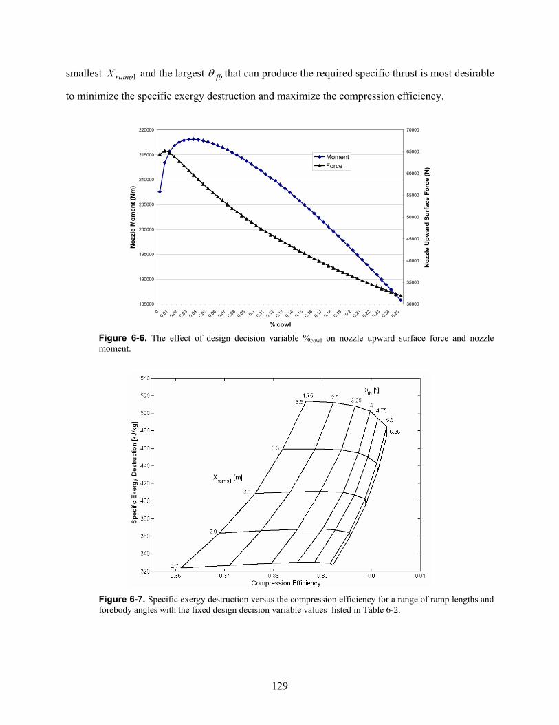
129

smallest 1rampX and the largest fbθ that can produce the required specific thrust is most desirable

to minimize the specific exergy destruction and maximize the compression efficiency.

185000

190000

195000

200000

205000

210000

215000

220000

00.0

10.0

20.0

30.0

40.0

50.0

60.0

70.0

80.0

9 0.1 0.11

0.12

0.13

0.14

0.15

0.16

0.17

0.18

0.19 0.2 0.2

10.2

20.2

30.2

40.2

5

% cowl

Noz

zle

Mom

ent (

Nm

)

30000

35000

40000

45000

50000

55000

60000

65000

70000

Noz

zle

Upw

ard

Surf

ace

Forc

e (N

)

MomentForce

Figure 6-6. The effect of design decision variable %cowl on nozzle upward surface force and nozzle moment.

Figure 6-7. Specific exergy destruction versus the compression efficiency for a range of ramp lengths and forebody angles with the fixed design decision variable values listed in Table 6-2.

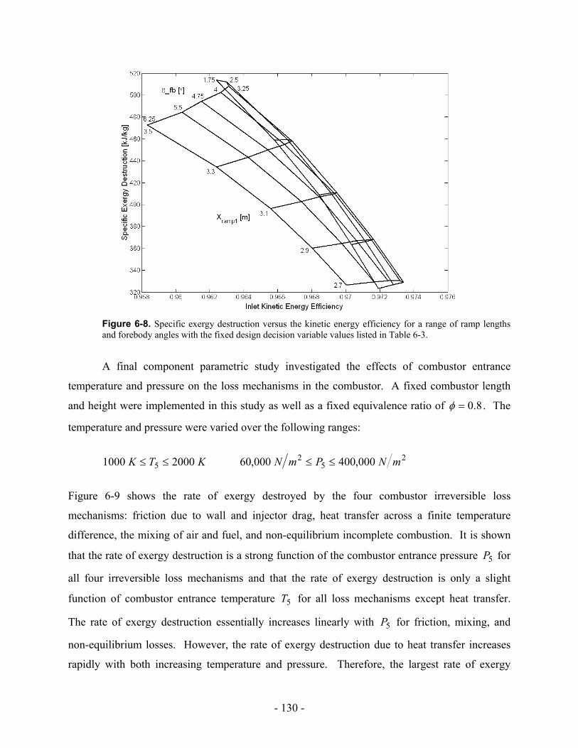
- 130 -

Figure 6-8. Specific exergy destruction versus the kinetic energy efficiency for a range of ramp lengths and forebody angles with the fixed design decision variable values listed in Table 6-3.

A final component parametric study investigated the effects of combustor entrance

temperature and pressure on the loss mechanisms in the combustor. A fixed combustor length

and height were implemented in this study as well as a fixed equivalence ratio of 8.0=φ . The

temperature and pressure were varied over the following ranges:

25

25 000,400000,6020001000 mNPmNKTK ≤≤≤≤

Figure 6-9 shows the rate of exergy destroyed by the four combustor irreversible loss

mechanisms: friction due to wall and injector drag, heat transfer across a finite temperature

difference, the mixing of air and fuel, and non-equilibrium incomplete combustion. It is shown

that the rate of exergy destruction is a strong function of the combustor entrance pressure 5P for

all four irreversible loss mechanisms and that the rate of exergy destruction is only a slight

function of combustor entrance temperature 5T for all loss mechanisms except heat transfer.

The rate of exergy destruction essentially increases linearly with 5P for friction, mixing, and

non-equilibrium losses. However, the rate of exergy destruction due to heat transfer increases

rapidly with both increasing temperature and pressure. Therefore, the largest rate of exergy

- 131 -

destruction due to heat transfer occurs at the highest combustor entrance temperature and

pressure (as expected from the combustor wall heat loss model of Section 4.1.2). Figure 6-9 also

reveals that non-equilibrium incomplete combustion losses are by far the most dominant loss

mechanism and heat transfer losses destroy the least rate of exergy.

Figure 6-9. Rate of exergy destroyed by combustor loss mechanisms at M5 = 3.2 and over a range of combustor entrance temperatures (T5) and pressures (P5). Molecular weights and specific heat ratio are fixed.

The results shown in Figure 6-9 are for a combustor entrance Mach number of 2.35 =M .

The aforementioned process was repeated for combustor entrance Mach numbers of

7.37.25 andM = as well and produced results exactly similar to those shown in Figure 6-9

except that magnitude of the exergy destruction rates varied (smaller at 2.7, larger at 3.7).

As mentioned in Section 4.1.2, the combustor model developed for this thesis does not

include the affects of molecular weight changes and specific heat ratio changes as more fuel is

being burned. Therefore, it was deemed important to account for molecular weight and specific

heat ratio changes in the combustor model in order to make comparisons of the flow properties

- 132 -

and irreversibilities with the combustor model that does not consider these changes. In order to

account for molecular weight and specific heat ratio changes and also their affects on the flow

properties, the mole fractions of each constituent in Equation (4.23) were calculated at each

combustor differential step and two additional terms were added to Equations (4.28) to (4.30)

(refer to [43]).

The above parametric study was repeated with molecular weight and specific heat ratio

changes in the combustor model for the same combustor geometry, equivalence ratio, and

combustor entrance ranges of temperature and pressure. The results of this study are shown in

Figure 6-10 where exergy destruction rates are once again plotted versus temperature and

pressure.

Figure 6-10. Rate of exergy destroyed by combustor loss mechanisms at M5 = 3.2 and over a range of combustor entrance temperatures (T5) and pressures (P5). Molecular weight and specific heat ratio changes are included in the combustor model.

As shown in Figure 6-10, the rates of exergy destruction due to friction and non-

equilibrium incomplete combustion increase linearly with pressure and are only slightly affect by

- 133 -

temperature. This happens to be the same trend previously depicted in Figure 6-9 for friction

and non-equilibrium incomplete combustion losses. It appears from a comparison of Figures 6-9

and 6-10 that accounting for molecular weight and specific heat ratio changes results in an

increase in frictional losses and decrease in mixing losses. It can also be seen from a comparison

of these two figures that heat transfer exergy destruction rates are identical for both combustor

models. This is once again attributed to the combustor wall heat loss model utilized in this work.

Finally, Figure 6-10 reveals that exergy destruction rates due to fuel/air mixing are affected

significantly by the inclusion of molecular weight and specific heat ratio changes in the

combustor model. At higher combustor entrance temperatures, the trend is essentially the same

as that shown in Figure 6-9; but as 5T decreases an increase in 5P tends to have a less significant

affect on the exergy destruction rates. In fact, at a low 5T there is not much difference in exergy

destruction rates for mixing at low or high 5P .

To further investigate this issue, three sets of combustor entrance properties (station 5)

were applied to a constant geometry and constant equivalence ratio combustor in order to

observe the influence molecular weight and specific heat ratio changes had on combustor exit

flow properties (station 6) and irreversibilities (i.e. entropy generation). The results of this

investigation are displayed in Table 6-3 where combustor B accounts for molecular weight and

specific heat ratio changes in the model. It can be seen that for all three sets of combustor

entrance conditions there are appreciable differences in the exit properties of the two combustor

models. From Table 6-3 it appears that a larger combustor entrance pressure results in a larger

difference between the exit pressures for combustors A and B. It is also evident from Table 6-3

the modifications applied to combustor model B result in significant changes to the entropy

generation rates from friction and mixing and these changes become more pronounced as the

combustor entrance Mach number increases. Combustor model B has only slight differences in

entropy generation rates due to non-equilibrium combustion compared to combustor model A

and there is no difference in entropy generation rates due to heat transfer between the two

models. In the end, combustor model B predicts about 5-10% smaller entropy generation rates

than combustor model A. Also, it can be concluded that a longer combustor for model B is

needed to obtain relatively similar combustor exit flow properties as determined from combustor

model A.

- 134 -

Table 6-3. Combustor affects due to molecular weight/specific heat ratio changes.

Station Comb. A Comb. B Comb. A Comb. B Comb. A Comb. B

5 2.5 2.5 3.2 3.2 3.9 3.9 M

6 1.171 1.660 1.567 2.009 1.751 2.241

5 1700 1700 1400 1400 1100 1100 T (K)

6 3222.8 2816.8 3089.4 2733.2 3020.5 2614.6

5 300000 300000 225000 225000 150000 150000 P

(N/m2) 6 895240 558950 692880 482760 561720 389360

5 1995 1995 2318 2318 2504 2504 u (m/s)

6 1288.1 1889.9 1693.9 2252.7 1882.7 2460.1

Friction 18.07 31.396 30.079 50.452 36.794 61.769

HT 4.294 4.294 4.305 4.305 3.452 3.452

Mixing 64.742 40.659 72.952 38.272 74.01 30.235

Irre

vers

ibili

ties

S irr

(kW

/K)

Inc. Comb. 181.79 177.17 184.99 180.09 161.72 155.63

The accuracy achieved with combustor model B is not without drawbacks. Each

combustor computation took approximately 0.5 seconds longer for combustor model B on a

single AMD Athlon 2.08 GHz processor with 992 MB of RAM. This doesn’t present much of a

problem for single point analysis. However, it may cause an additional computational burden

during optimizations because of the sheer number of runs (discussed shortly) and also because of

the throttling process of the vehicle.

6.3 Scramjet Engine Only Optimizations and Study

A study of a fixed geometry scramjet engine was conducted over a range of flight Mach

numbers in order to gain insights into the operation of the scramjet engine and the exergy

destruction of the propulsion sub-system components. This study investigated both a scramjet

engine that implemented energy exchange (see Section 4.1.1) with the freestream flow to

maintain the shock-on-lip condition and a scramjet engine with no energy exchange which

accounted for mass flow spillage at Mach numbers below the design value.

- 135 -

An approximation was utilized to determine that last streamline captured by the inlet and

calculate the mass flow spillage. First, the sum of the forebody and two ramp angles was

averaged to obtain an average flow angle. Next, a line was traced forward from the cowl lip at

the average flow angle until it intersected the forebody oblique shock (refer to Figure 3-15).

Finally, the area 0A was calculated which ultimately allowed for the calculation of the mass flow

spillage.

The scramjet engine used in this study operated at an equivalence ratio of 8.0=φ and a

design Mach number of 9=designM . Additionally, the flight Mach number range was

1170 toM = . The results of the analysis of the scramjet engine with and without energy

exchange are given in Table 6-4 and Figures 6-11 and 6-12.

Table 6-4. Scramjet engine with and without energy exchange.

0M 5M 5T

(K) 5P

(N/m2) Thrust

(N) airm&

(kg/s) Spillage

(kg/s)

←Q

(J/kg)

7 3.458 688.4 132130 92577 159.13 __ -61751

8 3.458 899.9 132080 68951 139.12 __ -33083

9 3.458 1141.6 131760 53061 123.22 __ 0

10 3.458 1413.8 130160 41993 109.38 __ 37504

Ene

rgy

Exc

hang

e

11 3.458 1716.3 129960 34444 99.128 __ 79430

7 3.133 808.4 106540 60758 108.81 50.32 __

8 3.343 953.3 114140 54921 113.5 25.26 __

9 3.458 1141.6 131760 53061 123.22 __ __

10 3.726 1259.6 115210 41795 109.38 __ __

No

Ene

rgy

Exc

hang

e

11 3.952 1392.2 104250 33810 99.128 __ __

The combustor entrance Mach number, temperature, and pressure for both the scramjet

engine with and without energy addition are given in Table 6-4. It shows that the scramjet

engine with energy exchange ( ←Q& ) maintains the same 5M for all flight Mach numbers (due

to the same inlet shock structure) and allows a small variation in 5P . This may be beneficial

- 136 -

from the standpoint that a scramjet combustor could be designed to operate for specific entrance

conditions. The scramjet engine that permits mass flow spillage has an appreciable variation in

both 5M and 5P over the flight Mach number range but has a much smaller variation in 5T in

comparison with the scramjet engine with energy exchange.

Table 6-4 also shows that at flight Mach numbers below the design value there are

significant losses in thrust due to mass flow spillage (which is approximately 30% of the

maximum capture value at 70 =M ). However, at 870 andM = there is power required to

operate some ‘device’ in order to exchange the required ←Q& which could negate some of the

additional thrust power achieved by using this device. For example, the thrust power at 70 =M

for the scramjet with energy exchange is kWPthrust 856,193= and equals kWPthrust 227,127=

for the scramjet without energy exchange. At this flight Mach number, the additional amount of

fuel required to operate this device is calculated from

−= ←

bairf T

TQmexm f

0

012&& (6.4)

where the exergy content of hydrogen fuel is kgkJex f 575,116= and it is assumed in

Equation (6.4) that twice as much energy is needed to operate the device as that being exchanged

with the flow (for illustration purposes). Therefore, the power required to operate the device is

determined to be kWPdevice 467,12= . One can, thus, be concluded that even though power is

needed to operate the device there is still a rather large benefit in terms of thrust power produced

for the scramjet engine with energy exchange.

At flight Mach numbers above the design value there is not much gain in thrust using the

energy exchange (while the device consumes power). However, this analysis did not account for

effects on the combustor from shock ingestion. Therefore, it may or may not be beneficial to

utilize energy exchange with the freestream flow at flight Mach numbers above the design value.

Figures 6-11 and 6-12 display the specific exergy destruction of each of the propulsion

sub-system components for the fixed geometry scramjet with and without ←Q& . The specific

exergy destruction of the inlet remains relatively constant over the flight Mach number range for

the scramjet with ←Q& . The specific exergy destruction of the inlet is smaller without ←Q& than

- 137 -

with ←Q& below the design Mach number and is larger without ←Q& than with ←Q& above the

design Mach number.

0

10

20

30

40

50

60

70

80

6 7 8 9 10 11 12

Flight Mach Number

Spec

ific

Exer

gy D

estr

uctio

n (k

J/kg

*K)

300

350

400

450

500

550

600

650

Spec

ific

Exer

gy D

estr

uctio

n (k

J/kg

*K)

(Com

bust

or &

To

tal)

InletEnergy AdditionNozzleCombustorTotal

Figure 6-11. Specific exergy destruction of the propulsion sub-system components over a range of flight Mach numbers. Energy exchange included in the propulsion sub-system.

The hypersonic vehicle propulsion system (i.e. scramjet engine) was optimized at flight

Mach numbers of 12,10,8,60 andM = and a fixed angle of attack of o0=α and equivalence

ratio of 7.0=φ . These optimizations were performed to investigate if any decision design

variable or other parameter trends exist between optimal scramjet engines at different flight

Mach numbers. The objective function maximized in these optimizations was the vehicle overall

efficiency, defined as

prf

o hmTu&

0=η (6.5)

- 138 -

which is a standard 1st Law based efficiency and is an indicator of how well the engine uses the

energy originally deposited in the fuel tanks [1]. The vehicle overall efficiency is often further

broken down into a thermal and propulsive efficiency68 defined by [1]

( )

( )

−+

⋅−+

=⋅=

221

221

20

27

0

20

27

uufm

Tufh

uuf

airpr

ptho

&

ηηη (6.6)

where f is the fuel/air ratio, u0 is the freestream velocity, and u7 is the velocity exiting the engine.

Also, note that these optimizations assume that the design Mach number is equivalent to the

flight Mach number.

0

20

40

60

80

100

120

6 7 8 9 10 11 12

Flight Mach Number

Spec

ific

Exer

gy D

estr

uctio

n (k

J/kg

*K)

0

100

200

300

400

500

600

700

Spec

ific

Exer

gy D

estr

uctio

n (k

J/kg

*K)

(Com

bust

or &

To

tal)

InletNozzleCombustorTotal

Figure 6-12. Specific exergy destruction of propulsion system components over range of flight Mach numbers. No energy exchange in propulsion system.

68 Thermal and propulsive efficiency calculations are only given in this section. They are not given in the last two sections of this chapter because when the airframe was incorporated into the optimizations unreasonable values were obtained for these to efficiencies. This was assumed to be a result of the fact that Equation (6.6) is not completely applicable to this work (see derivation of Equation (6.6) in [1]) and possibly due to the vehicle throttling method.

- 139 -

Anywhere from three to five optimization runs were made for each flight Mach number

depending on the precision of the objective function values. All optimizations were run to

40,000 function evaluations which took a few hours per run on a 2.79 GHz Pentium 4 processor

with 512 MB of RAM. In general, per flight Mach number, each optimization resulted in

relatively the same objective function value. However, the values of the design decision

variables for a given Mach number were not the same for each optimal solution. An example of

this is shown in Table 6-5 for the optimal Mach 10 solutions. The conclusion form this table is

that there are most likely quite a few configurations that produce relatively the same objective

function value (the inverse of Equation (6.5)). This implies that, for engine only optimizations,

the optimizer does a fairly good job of arriving at a solution in a region more than likely near the

global optimum but has trouble arriving exactly at it. This is not surprising since it is the nature

of EAs to get close but not exactly there. Thus, it would be beneficial to couple a gradient-based

method to the evolutionary algorithm to assist in arriving at the global optimum.

Table 6-5. Optimal Mach 10 scramjet configurations.

Run Obj. Fun. fbX cowlX 1rampX fbθ nozzθ combL cowl%

1 1.6225 8.4730 13.208 2.8042 3.3705 18.000 1.2080 0.0059

2 1.6049 8.5737 12.864 2.5221 5.0793 17.985 1.1000 0.0005

3 1.6274 8.5120 13.169 3.2046 4.8805 18.000 0.7267 0.0014

Nonetheless, a comparison of the optimal scramjet engines was made to investigate

trends and differences of design decision variables, other parameters, and exergy destruction

rates. To make a fair comparison, it was assumed that the global optimum was the minimum

objective function value for each flight Mach number. The results of the optimizations are

shown in Table 6-6 and Figures 6-13 and 6-14.

Table 6-6 lists the optimal values of the design decision variables for the optimal scramjet

engine at all four flight Mach numbers. Also listed in this table are the inlet length, overall

efficiency, thrust, contraction ratio, and air mass flow rate (listed in this order in Table 6-6).

Some noticeable trends for the optimal scramjet engines are as follows:

1. As 0M increases, fbX increases slightly and both cowlX and 1rampX decrease rather

substantially (relative to its overall magnitude). Consequently, these trends result in a

- 140 -

decrease in inlet length ( inletX ) as 0M increases. In fact, not only does the inlet length

become smaller as flight Mach number increases, the entire inlet itself becomes much

smaller. This can be seen in Appendix A where the optimal scramjet engine inlets at each

0M are drawn.

2. As 0M increases, both fbθ and CR increase significantly in order to compress the higher

Mach number flow to acceptable combustor entrance conditions.

Table 6-6. Optimal design decision variables and parameters for optimal scramjet engines.

Mach Number 6 8 10 12

Obj. Function 3.3948 1.9894 1.6049 1.4840

fbX 8.4005 8.4924 8.5737 8.7359

cowlX 16.285 13.633 12.865 12.154

1rampX 4.4432 3.0330 2.5222 1.9822

fbθ 1.8772 2.8273 5.0794 5.3887

nozzθ 17.942 17.811 17.985 17.993

combL 1.2519 1.1418 1.1000 1.0500

Des

ign

Dec

isio

n V

aria

bles

cowl% 0.0001 0.0003 0.0005 0.0002

inletX 17.769 14.442 13.444 12.622

oη 0.2942 0.5026 0.6243 0.6738

thη 0.2603 0.4692 0.5659 0.5888

pη 1.1304 1.0716 1.1033 1.1443

Thrust (N) 120430 79902 61681 40882

CR 9.6109 15.599 25.403 31.699 Oth

er P

aram

eter

s

airm& (kg/s) 296.61 154.91 121.15 89.895

3. combL decreases slightly as 0M increases (discussed more shortly). Therefore, this trend

along with the trends mentioned in 1. result in an increase in nozzle size as 0M increases.

- 141 -

4. The design variables nozzθ and cowl% are essentially at their maximum and minimum

allowable values, respectively, for all flight Mach numbers. This is because the

combination of these two variables, as mentioned, produces the largest thrust (refer to

Figure 6-5).

5. Even though the overall efficiency oη increases with increasing 0M , the thrust produced

by the engine decreases significantly. This is mainly the direct result of the high mass flow

rates at the low Mach numbers. Also, notice that there is an extreme jump in oη from the

optimal Mach 6 engine to the optimal Mach 8 engine. The low oη at Mach 6 is believed to

be a direct reflection of the fact that Mach 6 is sometimes considered the lower end of the

scramjet operating range. Not shown in Table 6-6 is the fact that as the flight Mach

number increases, the optimal scramjet engine operates at a higher combustor Mach

number, pressure, and temperature. Since differential changes in these properties in the

combustor are larger at higher combustor entrance conditions, a smaller combustor length

is needed as 0M increases in order to slow the flow down to its minimum allowable value

(essentially Mach 1).

0

20000

40000

60000

80000

100000

120000

6 8 10 12

Flight Mach Number

Exer

gy D

estr

uctio

n (k

W)

InletCombustorNozzleTotal

Figure 6-13. Rate of exergy destruction of the propulsion sub-system components for each of the optimal flight Mach number scramjet engines.

- 142 -

The exergy destroyed by each propulsion sub-system component for all four optimal

scramjet engines is displayed in Figure 6-13. Figure 6-14 is a more detailed breakdown of

Figure 6-13 where the exergy destroyed by each of the propulsion sub-system irreversible loss

mechanisms is shown69. Figure 6-13 shows that the exergy destroyed by the inlet component

decreases as the flight Mach number increases. This is what one would expect because the inlet

decreases in size with increasing 0M . The nozzle component shows a trend opposite to that of

the inlet, i.e. nozzle exergy destruction increases with flight Mach number. This is also as

expected because not only does the nozzle increase in size as 0M increases but the nozzle heat

loss rate also increases. Finally, Figure 6-13 shows that, in general, the combustor and total

exergy destruction both increase as 0M increases up to Mach 10. However, this could just be a

result of the assumptions made in this investigation. Even though combustor length decreases

slightly as 0M increases, the combustor exergy destruction should be expected to increase

because of operating at a larger Mach number, pressure, and temperature (refer to Figures 6-9

and 6-10).

0

10000

20000

30000

40000

50000

60000

6 8 10 12

Flight Mach Number

Exer

gy D

estr

uctio

n (k

W)

Inlet FrictionInlet ShocksComb FrictionComb Heat TransferComb MixingComb Non-EquilibriumNozzle

Figure 6-14. Exergy destruction due to individual loss mechanisms for each of the optimal flight Mach number scramjet engines.

69 The nozzle losses are not, in this case, broken down into heat transfer and friction losses. Refer to Section 4.1.3 for an explanation of the nozzle irreversibility calculation.

- 143 -

A final propulsion sub-system study completed for this work (and the most recent study

for this thesis work) was a comparison of the optimal scramjet engines determined from two

different objective functions. One objective function utilized in this investigation is the overall

efficiency given by Equation (6.5) which is maximized (or its inverse minimized). The second

optimization problem is

Minimize lossfueldes xExExf &&v +=)( (6.7)

where the second term on the right hand side of Equation (6.7) is the lost rate of exergy in

unburned fuel out the back of the vehicle (due to mixing losses). The purpose of the two

optimizations is to determine which objective function produces an engine (propulsion sub-

system) which consumes the least amount of fuel.

To make a justifiable comparison between these two objective functions, the engine was

required to produce 70,000 N of thrust. Therefore, this analysis allowed for throttling of the

equivalence ratio in order to provide the required thrust (explained in Section 4.2.5).

Additionally, the analysis was conducted for a flight Mach number of 80 =M and an angle-of-

attack of o0=α . A few optimization runs were made for both objective functions and the

optimal solution was simply the solution with the lowest objective function value. Each

optimization was run until it appeared to have converged70 to a solution which typically took

anywhere from 15,000-30,000 function evaluations. This resulted in computational times of

approximately 10-15 hours on a 2.79 GHz Pentium 4 processor with 512 MB of RAM.

The results of this analysis are given in Table 6-7 where the design decision variables are

shown along with the engine operating mass flow rate of fuel, the equivalence ratio, and the

vehicle volume produced by this engine. For this thesis work, Equation (6.5) is referred to as a

1st Law based objective function and Equation (6.7) as a 1st/2nd Law based objective function71.

Table 6-7 reveals that there are similarities between the design variables determined from the

optimization of the 1st and 1st/2nd Law objective functions. In fact, these similarities result in two

vehicles with almost identical volumes. Additionally, the two optimizations produced engines

70 The optimizations were stopped if the objective function value did not change for a few thousand evaluations. 71 In reference to the 1st and 2nd Laws of Thermodynamics.

- 144 -

that both operate at the same equivalence ratio and consume almost the same amount of fuel

(about a 1.5% difference between the two).

Table 6-7. Energy and exergy based optimizations for a scramjet engine with fixed thrust.

Obj. Function fbX cowlX 1rampX fbθ nozzθ

1st Law 8.6114 13.652 2.9049 4.6026 17.066

1st/2nd Law 8.4019 13.895 3.1784 4.5669 17.549

combL cowl% fm& (kg/s) φ veh∀ (m2)

1st Law 1.1148 0.0016 2.6363 0.5 26.039

1st/2nd Law 1.1523 0.0113 2.6754 0.5 26.025

The results of this analysis show that exergy methods possess the ability to determine the

optimal scramjet engine, i.e. the scramjet engine that consumes the least amount of fuel to

produce a required thrust. This can be concluded because the 1st Law objective function directly

minimizes fm& (the numerator is a fixed constraint in this analysis) and the 1st/2nd Law objective

function produces effectively the same fuel flow rate. It is also reasonable to conclude that if the

optimizer used work were coupled to an effective gradient-based search algorithm which could

focus in more precisely on the “global” optimum given the results of the EA for both objective

functions that the objective functions would produce fuel consumption rates ever closer to each

other. This is because the maximum power (ideal power) the engine is capable of producing is

equal to the sum of the thrust power, exergy destruction rate, and fuel exergy loss rate, i.e.

lossfueldesthrustff xExEPexm &&& ++= (6.8)

Since the thrust power is a fixed constraint, minimization of the exergy destruction rate and

exergy loss rate ultimately minimizes the fuel flow rate required to produce the necessary thrust.

An advantage of using the exergy-based measure given by Equation (6.7) for this

problem is that a detailed breakdown of all of the losses produced by each of the propulsion sub-

system loss mechanisms (for example, see Figure 6-14) can be used to provide insight into where

the largest improvements in engine performance can be realized. These improvements in engine

performance (by reduction of certain losses) ultimately allow a smaller mass flow rate of fuel to

- 145 -

be consumed to produce a fixed thrust. The vehicle overall efficiency provides no such insights

as to where improvements in the engine can be made to further reduce the amount of fuel being

consumed to produce the fixed thrust.

6.4 Single Mission Segment Optimizations and Partial Mission Optimizations

Single mission segment (i.e. single Mach number) optimizations and a partial mission

(consisting of three contiguous mission segments) optimization were performed for three

different objective functions. These optimizations were performed utilizing the entire hypersonic

vehicle model, i.e. propulsion sub-system and airframe sub-system. The single mission segment

optimizations correspond to each of the three segments (i.e. legs) of the partial mission. The

partial mission implemented for this thesis is given in Table 6-8. This partial mission was

deemed sufficient for verifying the proper operation of all the models and to seek solutions to all

three of the objectives72.

Table 6-8 shows that single mission segment optimizations were conducted for Mach 8

and Mach 10 cruise and Mach 8-10 acceleration where the flight Mach number is taken to be

90 =M . Both cruise mission segments required that DT = and the acceleration mission

segment required a certain thrust determined from Equation (3.1). The hypersonic vehicle was

required to have a fuel mass fraction of 15.0=fπ for the single segment cruise optimizations

and a fuel mass fraction of 10.0=fπ for the single segment acceleration optimizations73.

Additionally, the hypersonic vehicle operated at a design Mach number of 9=designM for all

single segment optimizations.

The two objective functions initially used to optimize all three single mission segments

were the vehicle overall efficiency and the total rate of exergy destruction, given by Equations

(6.5) and (6.3), respectively. The vehicle overall efficiency was maximized and the total rate of

exergy destruction was minimized for all optimizations. A third objective function implemented

in these optimizations was that defined by Equation (6.7) (for reasons to be discussed shortly).

72 As noted earlier a complete mission (see Figure 5-1) will be presented at the completion of the thesis work of K. M. Brewer anticipated for May 2005. 73 These two fuel mass fractions are arbitrarily chosen for this analysis.

- 146 -

Table 6-8. Partial mission specifications.

Segment Description




Several runs74 of the optimizer were performed for the each of the single segments using

the two initial objective functions. Only two runs of the optimizer were performed for both the

Mach 10 cruise segment and the Mach 8-10 acceleration segment using the objective function

defined by Equation (6.7) (due to time constraints). Once again, the minimum (or maximum,

depending on objective function) objective function value for each of the single segments was

assumed to be the “global” optimum for comparison and analysis purposes.

All of the single segment optimizations were carried out on a 2.79 GHz Pentium 4

processor with 512 MB of RAM. It took anywhere from 50,000-800,000 function evaluations

for the optimizer to find an initial feasible solution (i.e. a solution that does not violate any

constraints), which in of itself many hours75. Once a feasible solution was found, the

optimizations were carried out until the objective function did not change for at least 30,000

function evaluations76. A complete optimization of a single mission segment (one run of the

optimizer) typically took a day and a half. Unlike that for the propulsion sub-system

optimizations, each optimization run of a single segment did not produce relatively the same

objective function value, especially for the optimization of oη . It was concluded that the

optimizer for some of these runs was more than likely getting stuck at a local optimum. As

mentioned earlier, the coupling of a gradient-based method to the optimizer could alleviate this

problem. However, it was also concluded with some confidence that the lowest optimum value

of each objective function found for these single mission segment optimizations was either a

“global” optimum or a very good local optimum.

The results of single segment optimizations for all three objective functions are shown in

Tables 6-9 and 6-10. More specifically, Table 6-9 reveals the optimal values of the design

74 Usually 3-5 runs depending on the precision of the objective function values. 75 This problem was to be due to the fact that the optimizer generates random numbers to 16 significant digits. 76 It is possible but not probable that many evaluations later the optimizer may find a better solution. However, numerous tests revealed no evidence of this. Additionally, excessive computational times would occur for many more function evaluations.

- 147 -

decision variables (i.e. optimal vehicle configurations) determined by each objective function

and Table 6-10 displays values of calculated parameters such as exergy destruction rates, mass

flow rates, wing planform areas, vehicle volumes, etc. (parameters of interest).

Table 6-9. Design variable values for single segment optimizations.

Mach

#

Obj.

Funct. fbX cowlX 1rampX fbθ α nozzθ combL cowl%

0η 8.5303 12.619 2.4418 2.5501 1.7227 17.512 0.8933 0.0207 8

desxE& 8.4284 14.313 3.1839 1.0000 0.9547 15.524 0.5000 0.0736

0η 8.6716 13.616 3.2772 1.4914 1.2096 17.999 0.9451 0.0009

desxE& 8.4101 13.441 2.7657 1.0365 2.2349 17.335 0.5007 0.0860 8-10

lossfueldes xExE && + 8.5617 12.603 2.6580 1.0000 1.1521 12.8238 0.8802 0.2432

0η 8.4094 11.969 2.4620 1.7887 1.2450 15.842 0.7017 0.0136

desxE& 8.5113 14.267 3.0703 1.2493 0.9818 16.057 0.5003 0.2272 10

lossfueldes xExE && + 8.4127 13.265 3.2994 1.0577 1.7537 15.537 0.7775 0.2019

Table 6-9 shows that all optimizations resulted in vehicles in which the forebody length is

relatively close to its minimum allowable value of 4.8=fbX . In addition, the cowl position

always fell within 50-60% of the total vehicle body length. Optimal vehicle configurations tend

to have relatively small forebody deflection angles and angles-of-attack and rather large

expansion angles (in most cases). One significant finding in these optimizations and shown in

Table 6-9 is that minimization of the total rate of exergy destruction (Equation (6.3)) always

resulted in a vehicle with a combustor length essentially at its minimum allowable value of

5.0=combL . This obviously occurred because the combustor component exergy destruction

rates dominate the exergy destruction rates of the other components and because the shortest

combustor ultimately destroys the lease amount of exergy (this topic is revisited shortly since it

points to a deficiency in Equation (6.3) as the objective function). Another interesting result of

the optimizations shown in Table 6-9 is that optimal hypersonic vehicle configurations at these

- 148 -

flight Mach numbers have rather short combustors in terms of percent vehicle length (usually

less than 5% of vehL )77.

To obtain a better picture of the differences in the vehicle configurations predicted by

each of the objective functions, side portraits of the vehicle at each Mach number and for each

objective function are provided in Appendix B. For all the figures, the optimal vehicle

determined by the objective function 0η is plotted in blue. For Figures B-1, B-2, and B-4, the

optimal vehicle determined by the objective function desxE& is plotted in red. The optimal

vehicle determined by the objective function lossfueldes xExE && + is plotted in red in Figures B-3

and B-5. It can be seen from Figures B-1 and B-4 that the objective functions 0η and desxE&

produce much different Mach 8 and Mach 10 cruise vehicles. The cruise vehicles determined

from the optimization of desxE& tend to be much more slender and have larger inlets and smaller

nozzles. The accelerator vehicle configurations are very similar for these two objective

functions. Figure B-5 shows that minimization of lossfueldes xExE && + results in a more slender

vehicle as well when compared to the vehicle predicted by maximization of 0η . In addition, the

accelerator vehicles determined from 0η and lossfueldes xExE && + are fairly different (unlike the

case between 0η and desxE& ).

In the end, the optimal hypersonic vehicle configurations determined from minimization

of exergy destruction rates (Equation (6.3))or exergy destruction and exergy fuel loss rates

(Equation (6.7)) are smaller, more slender vehicles than optimal vehicles predicted by

maximization of the vehicle overall efficiency (Equation (6.5)). In addition, the center of gravity

of all the vehicles is more or less in the same location. These two statements are verified in the

figures in Appendix B and in Table 6-10.

Table 6-10 shows that short combustor lengths predicted by the exergy destruction

objective function resulted in a vehicle that consumes a considerable amount of more fuel for all

three single segments (this trend was also verified to occur for the partial mission). This was due

to the fact that the shorter combustors did not produce any significant combustion; and,

therefore, to produce appreciable thrust, the engine had to operate at higher equivalence ratios

77 This was true for all other optimization runs as well.

- 149 -

(even though the vehicles were smaller and more slender and less thrust was needed to balance

the drag or obtain the required thrust). Again, all of this points to a deficiency in Equation (6.3)

as the objective function.

Table 6-10. Calculated optimal parameter values for single mission segment optimizations.

Mach # 8 8-10 10

Obj.

Funct. 0η desxE& 0η desxE&

lossfuel

des

xE

xE&

& + 0η desxE&

lossfuel

des

xE

xE&

& +

airm& (kg/s) 121.82 119.56 105.20 95.084 92.460 84.700 96.134 84.944

fm& (kg/s) 0.6438 0.7021 1.8533 2.6801 1.6288 0.6963 0.9032 0.6983

φ 0.18 0.2 0.6 0.96 0.6 0.28 0.32 0.28

wingS (m2) 5.4834 0.0507 0.5028 0.0002 0.5025 9.2679 0.0097 0.0082

ω (°) 3.8000 4.8500 4.8800 4.7300 2.9100 4.8800 5.8200 4.8300

Inlet 9544.9 8377.1 9597.0 6380.7 9590.0 9337.6 6712.7 7909.4

Comb. 29467 16853 60714 23235 54782 32670 20575 32521

Nozzle 2251.5 1001.3 3912.4 2001.3 3939.7 5069.3 1838.9 3918.8

Aero* 9635.1 8320.1 9568.2 9587.1 9450.0 10652 9801.06 10094

Nrg* 563.02 552.61 0 0 0 277.33 314.77 278.1

Exe

rgy

Des

truc

tion

(kW

)

Total 51461 35104 83792 41203 75737 58007 39242 54722

veh∀ (m2) 26.171 18.750 23.966 22.856 18.351 24.052 19.735 21.081

cgx (m) 13.640 13.634 13.742 13.974 13.269 13.690 13.648 13.633

cgy (m) -0.0112 -0.2744 -0.0764 0.0645 -0.1537 0.1235 -0.2668 -0.0607

oη 0.4732 0.2015 0.5794 0.3780 0.5073 0.4422 0.1810 0.2886

lossfuelxE& 1515.8 23974 26951 213238 24891 2098.2 39064 2812.2

Thrust (N) 15212 7061.5 47493 44812 36549 12217 6487.6 7997.2

* Nrg refers to the the rate of exergy destruction resulting from the energy exchange with the inlet component flow. Aero refers to the airframe sub-system.

A breakdown of the exergy destruction rates of each component or sub-system (along

with that due to energy exchange) is given in Table 6-10. The table reveals that, in comparison

with the 0η objective function, the objective function desxE& did produce vehicles with smaller

- 150 -

components/sub-system exergy destruction rates. In fact, the total exergy destruction rates were

approximately 32% less for the optimal desxE& cruise vehicles and almost 50% less for the

optimal desxE& accelerator (compared to the optimal 0η vehicles). For the optimal 0η cruise

vehicles, however, the fuel exergy loss rates were only about 5% of the optimal desxE& vehicles

and for the optimal 0η accelerator, the fuel exergy loss rates were approximately 13% of the

optimal desxE& vehicle.

A comparison of the results of the 0η and desxE& optimizations provides much insight

with the conclusion that minimization of the exergy destruction rate is simply insufficient in

determining a hypersonic vehicle configuration that consumes the least amount of fuel to

produce the thrust for a given mission. It was recognized that not only is minimization of the

exergy destruction rate desirable, but so is minimization of the fuel exergy loss rate in unburned

fuel and, therefore, must be included in the objective function.

Table 6-10 reveals that minimization of lossfueldes xExE && + resulted in a Mach 10 cruise

vehicle that consumes essentially the same amount of fuel as the optimal 0η Mach 10 cruise

vehicle. The sum of the exergy destruction and exergy loss for the optimal lossfueldes xExE && +

vehicle is only about 4% less than that for the optimal 0η vehicle. Further investigation of Table

6-10 reveals that the optimal 0η vehicle produces substantially more thrust power (at Mach 10,

smu 2.30230 = ) than the optimal lossfueldes xExE && + vehicle. The previous two statements

along with Equation (6.8) point to the fact that the optimal 0η vehicle should actually consume

more fuel than the optimal lossfueldes xExE && + vehicle. The fuel mass flow rates predicted by

Equation (6.8) and using the values from Table 6-10 are skgm f 7410.00 =⇒ &η and

skgmxExE ffueldes loss 6143.0=⇒+ &&& . These flow rates78 compared to those for fm& in Table

6-10 show that the fuel mass flow rate determined by the hypersonic vehicle model does not

always correspond exactly to that required in Equation (6.8). It is understood that these

discrepancies are probably due to a number of things such as assumptions made in component

78 The tabulated mass flow rates are the mass flow rates required to produce the thrust power and overcome the rates of exergy destruction and fuel exergy loss listed in Table 6-10, i.e. these mass flow rates are more representative of the truth.

- 151 -

models, vehicle throttling methods, inexact prediction of the irreversibilities, etc. However,

these discrepancies do not undermine the comparison of these two optimal vehicles and, if

anything, substantiate the fact the optimal lossfueldes xExE && + vehicle consumes less fuel at Mach

10 cruise.

A comparison is also made in Table 6-10 between the optimal accelerator vehicles

determined from the vehicle overall efficiency and the exergy destruction and exergy fuel loss

objective functions. Table 6-10 shows that the optimal lossfueldes xExE && + accelerator has lower

exergy destruction rates and fuel exergy loss rates as well as smaller thrust power production.

Consequently, this vehicle consumes an appreciable less amount of fuel (about 12% less) than

the optimal overall efficiency vehicle. For the accelerator vehicle, the sum of the exergy

destruction and fuel exergy loss for the optimal lossfueldes xExE && + vehicle is approximately 10%

less than that for the optimal 0η vehicle. Once again using Table 6-10 along with Equation (6.8)

(at Mach 9, smu 1.27120 = ), the mass flow rates for the two objective functions are

skgm f 9728.10 =⇒ &η (6.5% larger than in the Table 6-10) and

skgmxExE ffueldes loss 6324.1=⇒+ &&& (0.2% larger than in the Table 6-10). This again further

emphasizes the fact that the optimal lossfueldes xExE && + accelerator consumes less fuel than the

optimal 0η vehicle .

A few other interesting results can be seen in Table 6-10. For example, the table shows

that using either of the exergy objective functions results in a vehicle requiring almost no

additional planform area to provide the necessary vehicle lift whereas the vehicle overall

efficiency objective function sometimes results in a vehicle with considerable planform areas. It

also appears that for all the optimal vehicles, the elevon deflection angle is rather minimal and

the center of gravity of the vehicles tend to be along the vehicle reference axis at a location

almost always near 57% of vehL . Finally, it is shown that cruise vehicles operate at rather low

equivalence ratios.

After analyzing the results of the single segment optimizations it can be concluded that

minimization of the exergy destruction and fuel exergy loss rates minimizes the amount of fuel

consumed by a hypersonic vehicle for a given mission beyond that which maximization of the

- 152 -

vehicle overall efficiency achieves. It can further be concluded from these analyses that the

acceleration segment of the partial mission will most likely dictate the vehicle design because

this is where the largest rates of exergy destruction and fuel exergy loss occur.

Lastly, a three-dimensional solid model for a typical Mach 10 hypersonic cruise vehicle

is given in Figure 6-15 to provide a clearer image of the hypersonic vehicle configurations

implemented in this thesis work.

Figure 6-15. 3D CAD representation of a typical Mach 10 hypersonic cruise vehicle.

With the partial mission defined in Table 6-8, an estimation was made of the initial total

mass (empty mass + fuel mass) of the hypersonic vehicle using Equations (4.86)-(4.89). In

determining the fuel mass fractions for each mission segment, the initial and final velocity and

elevation were determined from knowledge of the constant dynamic pressure trajectory. Also,

prediction of the estimated fuel mass fractions required estimation of the vehicle overall

efficiency and lift-to-drag ratio of the vehicle. For this analysis, the vehicle average overall

efficiency and lift-to-drag ratio were estimated to be 35.00 =η and 0.4=DL over the whole

mission. Based on these values, the fuel mass fractions for each of the mission segments are

given in Table 6-11. In addition to these fuel mass fractions, a fuel mass fraction of 06.0=fπ

was added to the vehicle to represent some amount of fuel that is required to return the vehicle to

its origin (or destination). Therefore, it is evident that for this partial mission analysis, the

- 153 -

hypersonic vehicle requires an estimated 30.69% of its initial mass to be fuel. Once a vehicle

volume is determined, the estimated initial mass of the vehicle can be calculated79.

Table 6-11. Mission segment fuel mass fractions.

Segment Fuel Mass Fraction, fπ

0 0.1025

1 0.0419

2 0.1025

∑2

0fπ 0.2469

At the end of each mission segment, the mass flow rate of fuel required for that segment

is known. Therefore, with knowledge of both the mission segment time and fuel flow rate, the

mass of the vehicle at the end of each mission segment can be determined. This updated vehicle

mass becomes the mass for the next mission segment. At the end of the mission, the amount of

fuel needed to complete the mission is known and can be compared to the initial prediction.

Realistically, if there is an appreciable percent difference between the initial prediction and the

calculated value, the mission would be re-run with the same vehicle but now using the calculated

total fuel mass fraction. This iterative process would be repeated until convergence. However,

to reduce the computational burden, this method was not incorporated for this thesis work. The

consequences of doing so are discussed following Table 6-15 below where a comparison of the

initial total fuel mass fraction and the calculated total fuel mass fraction will be given in the

mission results.

All of the partial mission optimizations were carried out on a single AMD Athlon 2.08

GHz processor with 992 MB of RAM. It took anywhere from 200,000 function evaluations to

sometimes over 1 million function evaluations to find an initial feasible solution. Once an initial

feasible solution was found, the optimizations were carried out until the objective function value

did not change for several thousand evaluations. However, the optimizations were only

discontinued at this point if the objective function had already progressed through a series of

minimizations. Usually less than 20,000 function evaluations were conducted once an initial

79 Note that the empty mass of the vehicle is scaled based upon the vehicle volume. See Section 4.2.4.

- 154 -

feasible solution was found80. This was because computational times became quite excessive.

The first few thousand evaluations, once an initial solution was found, proceeded relatively

quickly. However, as more and more feasible solutions were discovered, the computational

times became much larger. Typically, after 8,000 function evaluations past the initial feasible

solution, computational times became around 9-12 hours per 1,000 evaluations. For this reason,

the optimizations were ended if the objective function value did not change for several thousand

evaluations.

Optimizations were once again conducted using the same three objective functions as in

the single segment optimizations. The results of the mission optimizations are given in

Tables 6-12, 6-13, and 6-14. Table 6-12 presents the optimal design decision variables, Table 6-

13 the operational decision variable values in each of the mission segments, and Table 6-14

displays other optimal parameter values which were deemed pertinent to the following

discussion. Results are presented for the desxE& objective function in all three tables to further

emphasize its inability to provide more desirable configurations, i.e. it predicts instead shorter

combustor lengths and larger fuel consumption rates. Consequently, further comparisons with

the other two objective functions are not included in the remaining discussion.

It can be seen that, as with the optimal single mission segment vehicles, the optimal

mission vehicles have forebody lengths that are relatively close to the minimum value and the

cowl position falls within the same range described earlier. The optimal mission vehicles also

have small forebody angles and seem to require, in general, small nozzle expansion angles when

optimized for a mission. Table 6-12 shows that the optimal lossfueldes xExE && + vehicle has a

substantially larger combustor length and nozzle cowl extension than the optimal 0η vehicle.

Some of these traits can be seen in Appendix C where the optimal 0η vehicle is plotted in blue

and the optimal lossfueldes xExE && + vehicle is plotted in red. It is shown that the optimal

lossfueldes xExE && + vehicle is more slender and has a slightly larger inlet and a smaller nozzle.

Since the vehicle is more slender, the vehicle volume is less (length the same), and it

consequently has a smaller empty mass as shown in Table 6-14.

80 The optimizations progressed much more rapidly for the mission than for the single segment.

- 155 -

Table 6-12. Optimal design decision variable values for the partial mission.

Objective

Function fbX cowlX 1rampX fbθ nozzθ combL cowl%

0η 8.4371 13.186 3.2913 1.2179 15.835 0.6385 0.0010

desxE& 8.5021 13.667 2.7605 1.0017 15.889 0.5067 0.0115

lossfueldes xExE && + 8.8604 13.959 3.2978 1.0176 14.106 0.8240 0.1610

Table 6-13 shows that the optimal 0η vehicle fly’s at larger angles-of-attack throughout

the mission. It also shows that the optimal 0η vehicle requires much larger planform areas to

provide the necessary lift at each mission segment. It is concluded from these results and the

results of the single mission segment optimizations that the optimal vehicles have small angles-

of-attack because of their influence on the performance of the inlet component.

Table 6-13. Optimal operational decision variable values for the partial mission.

Objective

Function α wingS

0 1 2 0 1 2

0η 1.7724 1.2 0.9 7.2033 5.7615 9.3670

desxE& 1.4453 0.8 0.8 7.6983 9.2350 0.4869

lossfueldes xExE && + 1.1933 0.4 0.3 0.7908 3.2372 0.5065

Table 6-14 reveals that the optimal lossfueldes xExE && + vehicle consumes less fuel at each

of the mission segments in comparison to the optimal 0η vehicle. It consumes approximately

6%, 17%, and 2% less for mission segments 0, 1, and 2, respectively, and for the entire mission it

consumes about 6.5% less (70 kg). Table 6-14 also shows that both optimal vehicles require a

larger mass flow rate of fuel than that which is being injected into the combustor to cool the

combustor and nozzle surfaces (a result of larger heat loads at higher Mach numbers) for the

Mach 10 cruise segment. The additional 6% of initial vehicle weight carried during the mission

provides enough extra fuel to allow the necessary cooling for both vehicles. It is apparent that

vehicle cooling requirements are a serious hypersonic vehicle synthesis/design consideration.

- 156 -

Table 6-14. Calculated optimal parameter values at each segment of the partial mission.

Obj.

Funct. oη

lossfuel

des

xE

xE&

& + desxE&

Segment 0 1 2 0 1 2 0 1 2

airm& (kg/s) 109.35 96.875 86.004 115.67 102.47 90.961 111.91 99.138 88.005

fm& (kg/s) 0.5779 2.3892 0.7070 0.5434 1.9856 0.6944 0.7228 2.7943 0.8269

needfm& (kg/s) 0.5012 0.7416 0.9995 0.4996 0.7473 0.9997 0.1998 0.2942 0.3917

emptym (kg) 4374.4 3568.6 4093.5

fuelm (kg) 445.50 215.03 433.1 418.91 178.70 425.39 556.21 251.49 506.56

φ 0.18 0.84 0.28 0.16 0.66 0.26 0.22 0.96 0.32

Inlet 10372 9251.9 8267.1 10411 9286.2 8296.9 7950.2 7091.6 6336.2

Comb 24540 48843 30544 25121 52162 31638 17306 22535 19833

Nozzle 2403.5 4215.1 4161.2 1836.2 3255.9 3229.5 1098.8 1821.0 1947.5

Aero* 8669.9 9420.1 10171 8504.7 9302.4 9874.7 8534.7 9343.4 9915.9

Nose 505.42 15.282 128.28 534.64 44.161 111.66 517.25 24.824 157.92

Nrg

*

Ramp 0 50.931 97.277

0 120.61 132.51

0 71.299 63.704

Exe

rgy

Des

truc

tion

(kW

)

Total 46492 71794 53368 46409 74173 53284 35407 40889 38254

lossfuelxE& (kW) 2018.4 97165 4697.6 1515 53687 3922.4 23935 228780 33461

Thrust (N) 12748 50511 10521 7845.2 39996 5666.0 9174.4 46302 7520.9

oη 0.4418 0.4779 0.3750 0.2892 0.4554 0.2056 0.2545 0.3747 0.2295

veh∀ (m2) 21.872 17.843 20.467

calcfπ 0.0815 0.0393 0.0792 0.0912 0.0389 0.0926 0.1029 0.0465 0.0937

* Nrg refers to the rate of exergy destruction resulting from the energy exchange with the inlet component flow. Aero refers to the airframe sub-system.

The values of the thrust power (at Mach 8, smu 5.24020 = ) and rates of exergy

destruction and fuel exergy loss given in Table 6-14 were once again used in conjunction with

Equation (6.8) to calculate the mass flow rate of fuel required to supply the thrust power and

overcome exergy destruction rates and fuel exergy loss. These calculated mass flow rates are

compared to the model mass flow rates for both optimal vehicles in Table 6-15. It is apparent

that once again there are some discrepancies in these values but, if anything, only substantiate

the conclusions already drawn.

- 157 -

Table 6-15. Vehicle optimal fuel mass flow rate comparison.

Segment lossfueldes xExE && + 0η

Calculated fm& Model fm& Calculated fm& Model fm&

0 0.4998 0.5434 0.6045 0.5779

1 1.9475 1.9856 2.5437 2.3892

2 0.5529 0.6944 0.6836 0.7070

Table 6-14 also shows that the optimal lossfueldes xExE && + vehicle has less rates of exergy

destruction in only the nozzle component and the airframe sub-system only in comparison with

the optimal 0η vehicle. In fact, the optimal lossfueldes xExE && + vehicle has a larger rate of exergy

destruction during the acceleration segment and only slightly lower rates of exergy destruction

during both cruise segments. However, the rates of fuel exergy loss for the optimal

lossfueldes xExE && + vehicle are approximately 25%, 45%, and 17% less for segments 0, 1, and 2,

respectively. It is worth noting that even though the sum of the exergy destruction and fuel

exergy loss rates are smaller for the optimal lossfueldes xExE && + vehicle, it still is less efficient

transforming energy in the fuel tank to useful propulsive work.

For the partial mission analysis, minimizing the rates of exergy destruction and fuel

exergy loss produce a more optimal vehicle in terms of fuel consumption than maximizing the

vehicle overall efficiency. This is because the vehicle overall efficiency is only concerned with

production of vehicle thrust and does not account for the additional degrees of freedom of the

airframe sub-system (see [70]). The exergy-based measure does account for the degrees of

freedom of the airframe by calculating the rates of exergy destruction produced by external

aerodynamic surface shear forces. Since all the vehicle losses are determined in terms of a

common metric (i.e. exergy destruction rates), the losses occurring in the vehicle sub-systems

and components can be compared to identify the location of where the largest improvements in

vehicle performance can be made.

Tables 6-16 and 6-17 show the effectiveness of the optimizations performed using the 0η

and lossfueldes xExE && + for the partial mission. More specifically, these tables show a comparison

of the initial solution found by the optimizer and the final optimal solution for both objective

- 158 -

functions (as given in Table 6-14). Table 6-16 reveals that the for lossfueldes xExE && + objective

function significant decreases in the fuel consumption rates and fuel exergy loss rates have been

accomplished through optimization and appreciable decreases in exergy destruction rates have

occurred as well. Table 6-17 shows that for the 0η objective function fuel mass flow rates

decreased substantially and the vehicle overall efficiency increased significantly at each mission

segment.

Table 6-16. Comparison of initial feasible vehicle and final

optimal vehicle using the exergy objective function.

Objective Function

lossfuel

des

xE

xE&

& +

Initial Value Final Value Obj. Funct. Value 368764 232990

0 0.8184 0.5434 1 3.0613 1.9856 fm&

(kg/s) 2 1.0012 0.7473 0 9108.3 1515 1 152900 53687 lossfuelxE&

(kW) 2 16439 3922.4 0 53691 46492 1 76533 74173 totaldesxE&

(kW) 2 60089 53284

Table 6-17. Comparison of initial feasible vehicle and final optimal vehicle using the overall efficiency objective function.

Objective Function oη

Initial Value Final Value Obj. Funct. Value 3.5720 2.317

0 0.7156 0.5779 1 2.7241 2.3892 fm&

(kg/s) 2 0.8898 0.7070 0 0.2608 0.4418 1 0.3771 0.4779 oη 2 0.2020 0.3750

It can be seen it Table 6-14 that the actual total fuel mass fraction (sum of segments 0, 1,

and 2) is less than that predicted in Table 6-11 for both vehicles (10% less for the optimal

lossfueldes xExE && + vehicle and 20% less for the optimal 0η vehicle). Therefore, the iterative

process described earlier would be beneficial for obtaining more exact values in Table 6-14.

This iterative process could have some impacts on the final results shown in Table 6-14

- 159 -

depending on the magnitude of the difference between the actual fuel mass fraction and the

estimated fuel mass fraction. Impacts such as larger/smaller planform areas could conceivably

require larger/smaller thrust requirements which ultimately influence fuel consumption rates.

However, even a 10% error (or possibly more) like that encountered in this thesis work may only

slightly influence the planform size and, consequently, may produce no change in the fuel

consumption rates (due to the throttling process used in this thesis work). Nonetheless, the

iterative process is worth considering for future mission optimizations.

Finally, a number of simplifications were made to the sub-system and component models

to achieve the desired objectives within the context of one-dimensional analysis and as a result of

computational restrictions. This thesis work strived towards the development and presentation of

theory (i.e. demonstration of methodology) and not the prediction of ‘exact’ vehicle operating

conditions, parameter values, etc. Therefore, the reader should take caution when considering

the conclusions and some of the parameter values presented in the tables with respect to real

hypersonic vehicles.

- 160 -

Chapter 7

Conclusions

A number of conclusions can be drawn from the various parametric studies and

optimizations performed as well as from the work that led up to the production of the results in

Chapter 6. The main conclusions derived from the results of this research are summarized as

follow:

1. Hypersonic aircraft systems are highly dynamic, integrated vehicles which are subjected

to a wide array of flight conditions. Sufficiently accurate physical, thermodynamic, and

aerodynamic models are required to predict the performance of these systems over the

flight spectrum with any confidence. Sufficiently accurate models were developed for

this thesis work which permitted good predictions of performance as well as of

irreversibilities due to the various hypersonic vehicle system loss mechanisms.

2. The evolutionary algorithm (EA) optimization software utilized in this thesis work had a

number of benefits and drawbacks. The EA required no initial guess of the design

decision variables and possessed the ability to optimize the large-scale hypersonic vehicle

mission problem. However, long computational times, which, of course, are the nature of

the EA optimization approach, occurred for both single mission segment and partial

mission optimizations, suggesting that more computational power may be needed in the

future. Furthermore, re-optimizing only sometimes repeated the previous solution

sufficiently well to validate it as the best to be found. As previously mentioned, this

particular problem can be alleviated to a large extent through the coupling of a gradient-

based method with the evolutionary algorithm, i.e. by feeding the final solution of the EA

to the gradient-based method so that it can use this solution as its initial point and zoom

in on what is thought to be the “global” solution.

- 161 -

3. Scramjet engine investigations show that as expected the combustor component is the one

with the largest rates of exergy destruction. Consequently, the design of the combustor

component requires a great deal of attention, especially focusing on providing efficient

mixing and burning at high flow velocities. It was shown that the combustor irreversible

loss mechanisms are largely affected by combustor entrance properties and, therefore, an

inlet must provide desirable conditions to the combustor over a large range of flight

conditions.

4. Optimizations on a fixed-geometry scramjet engine only were conducted over a range of

Mach numbers in order to determine the effects of maintaining the shock-on-lip condition

at design and off-design through energy exchange with the free stream at two-points prior

to the entrance of the engine inlet. These results were then compared with the

performance of the same engine without energy exchange. The results seem to indicate

that even with a device which provides or extracts energy from the free stream at an

efficiency of only 50%, that the benefits in terms of thrust gain are quite substantial over

those for an engine without such a device.

5. Optimizations were performed for the propulsion sub-system only at a number of flight

Mach numbers using the overall vehicle efficiency as the objective function. These

optimizations revealed a number of trends, most notably, a decrease in the inlet

component size as the flight Mach number increased and a rather large increase in the

overall vehicle efficiency as the flight Mach number increased. Another result of these

optimizations was an appreciable increase in the rate of exergy destruction as the flight

Mach number increased from Mach 6 to Mach 12.

6. An exergy-based method (i.e. the thermodynamic effectiveness) was shown to be able to

predict essentially the same optimal combustor length as a thrust-based measure (i.e. the

engine effectiveness) in terms of thrust production. The application of this exergy-based

method to the design optimization of a hypersonic propulsion sub-system only resulted in

a scramjet engine configuration that consumed the least amount of fuel to maintain a

given thrust. Thus, minimization of the rate of exergy destruction due to the irreversible

loss mechanisms present in the engine and the rate of fuel exergy loss due to incomplete

mixing gave a scramjet configuration that effectively consumed the same amount of fuel

- 162 -

as a scramjet that was optimized for minimum fuel usage. The use of a gradient-based

method coupled to the EA would have only further confirmed this result by producing

identical fuel consumption rates for the two optimal engines.

7. Single mission segments and a partial, three-segment mission were optimized for three

different objective functions; namely, the overall vehicle efficiency, 0η , the rate of

exergy destruction desxE& , and the rate of exergy destruction plus fuel exergy loss

lossfueldes xExE && + . It was shown for both single mission segment optimizations and the

partial mission optimization that desxE& produced undesirable optimal configurations

because of its tendency to arrive at a vehicle configuration with the smallest allowable

combustor length. However, adding the rate of fuel exergy loss to the rate of exergy

destruction, i.e. lossfueldes xExE && + , resulted in an optimal vehicle for the partial mission

that consumed less fuel than the optimal partial mission vehicle determined from the 0η

optimization. In fact, a 6.5% smaller amount of fuel was consumed by the optimal

lossfueldes xExE && + vehicle in comparison with the optimal 0η vehicle. It was further

concluded that a larger savings in fuel consumption more than likely will be realized

when these two objective functions are evaluated for a more complete mission (e.g., the

one given in Figure 5.1).

8. This thesis work presented one of the first known totally integrated hypersonic vehicle

concept optimizations throughout a hypersonic mission. An exergy-based measure

produced a more optimal vehicle in terms of fuel consumption than a standard hypersonic

vehicle performance measure (the vehicle overall efficiency). This is because the overall

efficiency is only concerned with thrust production and does not consider the additional

degrees of freedom of the airframe sub-system. The exergy-based measure does account

for the airframe sub-system degrees of freedom through calculation of surface shear force

exergy destruction rates. Additionally, quantifying all the vehicle losses in terms of rate

of exergy destruction provides a common metric for the vehicle designer to identify

where the largest improvements in vehicle performance can be made which ultimately

result in a lower amount of fuel consumption.

- 163 -

Appendix A

Figure A-1. Optimal inlet component configurations for the scramjet engine (propulsion sub-system) only optimizations.

- 164 -

Appendix B

Figure B-1. Optimal Mach 8 cruise vehicles for the single segment optimizations using the objective functions ηo and Exdest . Both the vehicle plumes and centers of gravity are shown in the figure.

- 165 -

Figure B-2. Optimal Mach 8-10 accelerator vehicles for the single segment optimizations using the objective functions ηo and Exdest . Both vehicle plumes and centers of gravity are shown in the figure.

- 166 -

Figure B-3. Optimal Mach 8-10 accelerator vehicles for the single segment optimizations using the objective functions ηo and Exdest + Exloss. Both vehicle plumes and centers of gravity are shown in the figure.

- 167 -

Figure B-4. Optimal Mach 10 cruise vehicles for the single segment optimization using the objective functions ηo and Exdest . Both vehicle plumes and centers of gravity are shown in the figure.

- 168 -

Figure B-5. Optimal Mach 10 cruise vehicles for the single segment optimization using the objective functions ηo and Exdest + Exloss. Both vehicle plumes and centers of gravity are shown in the figure.

- 169 -

Appendix C

Figure C-1. Optimal partial mission vehicles for objective functions ηo and Exdest + Exloss.

- 170 -

References

[1] Heiser, W. H., and Pratt, D. T., Hypersonic Airbreathing Propulsion, AIAA, Inc., Washington, D.C., 1994.

[2] Anderson Jr., J. D., Hypersonic and High Temperature Gas Dynamics, AIAA, Inc., Reston, VA, 1989.

[3] Anderson Jr., J. D., Fundamentals of Aerodynamics, 3rd Edition, McGraw-Hill, New York, 2001.

[4] Moorhouse, D. J., “Proposed System-Level Multidisciplinary Analysis Technique Based on Exergy Methods”, Journal of Aircraft, Vol. 40, No. 1, January-February 2003.

[5] Moorhouse, D. J., and Suchomel, C. F., “Exergy Methods Applied to the Hypersonic Vehicle Challenge”, AIAA Paper No. 2001-3063, 2001.

[6] Moorhouse, D. J., Hoke, C. M., and Prendergast, J. P., “Thermal Analysis of Hypersonic Inlet Flow with Exergy-Based Design Methods”, International Journal of Applied Thermodynamics, Vol. 5, No. 4, December 2002.

[7] Camberos, J. A., and Moorhouse, D. J., “Modeling Aerospace Vehicle Systems Based on Minimum Exergy Destruction”, First International Conference on Grand Challenges for Modeling and Simulation, draft version.

[8] Camberos, J. A., “Quantifying Irreversible Losses for Magnetohydrodynamic (MHD) Flow Simulation”, AIAA Paper 2003-3647, 2003.

[9] Riggins, D. W., “High-Speed Engine/Component Performance Assessment Using Exergy and Thrust-Based Methods”, NASA Contractor Report 198271, 1996.

[10] Riggins, D. W., McClinton, C. R., and Vitt, P. H., “Thrust Losses in Hypersonic Engines Part 1: Methodology”, Journal of Propulsion and Power, Vol. 13, No. 2, March-April 1997.

[11] Riggins, D. W., “Thrust Losses in Hypersonic Engines Part 2: Applications”, Journal of Propulsion and Power, Vol. 13, No. 2, March-April 1997.

[12] Riggins, D. W., “Evaluation of Performance Loss Methods for High-Speed Engine and Engine Components”, Journal of Propulsion and Power, Vol. 13, No. 2, March-April 1997.

[13] Riggins, D. W., Taylor, T., and Homan, K., “The Detailed Auditing and Optimization of High Speed Vehicle Performance in Terms of Irreversibility and Heat”, Summer Research Presentation at Air Force Research Laboratories, July 2004.

- 171 -

[14] Roth, B. A., “A Work Potential Perspective of Engine Component Performance”, AIAA Paper 2001-3300, 2001.

[15] Roth, B. A., and Mavris, D. N., “Generalized Model for Vehicle Thermodynamic Loss Management”, Journal of Aircraft, Vol. 40, No. 1, January-February 2003.

[16] Figliola, R. S, Tipton, R., and Li, H., “Exergy Approach to Decision-Based Design of Integrated Aircraft Thermal Systems”, Journal of Aircraft, Vol. 40, No. 1, January-February 2003.

[17] Figliola, R. S., Stewart, J., Nomura, S., and Camberos, J. A., “An Exergy Based Methodology for Aircraft Systems Integration: Wing Aerodynamics Assessment”, Summer Research Presentation at Air Force Research Laboratories, July 2004.

[18] Paulus Jr., D. M., and Gaggioli, R. A., “Rational Objective Functions for Vehicles”, AIAA Paper No. 2000-4852.

[19] Bejan, A., “Architecture From Exergy-Based Global Optimizaiton: Tree-Shaped Flows and Energy Systems for Aircraft”, AIAA Paper No. 2000-4855, 2000.

[20] Bejan, A., “Constructal Theory: Tree-Shaped Flows and Energy Systems for Aircraft”, Journal of Aircraft, Vol. 40, No. 1, January-February 2003.

[21] Curran, E. T., and Murthy, S. N. B., Scramjet Propulsion, Progress in Astronautics and Aeronautics, Vol. 189, AIAA, Inc., Reston, VA, 2000.

[22] Curran, E. T., and Craig, R. R., “The Use of Stream Thrust Concepts for the Approximate Evaluation of Hypersonic Ramjet Engine Performance”, Air Force Aero-Propulsion Laboratory, Tehcnical Report AFAPL-TR-73-38, July 1973.

[23] Czysz, P., and Murthy, S. N. B., “Energy Analysis of High-Speed Flight Systems”, High Speed Flight Propulsion Systems, edited by S. N. B. Murthy and E. T. Curran, Progress in Astronautics and Aeronautics, Vol. 137, AIAA, Inc., Reston, VA, 1991.

[24] Gyftopoulos, E. P., and Beretta, G. P., Thermodynamics: Foundations and Applications, Macmillan Publishing Co., New York, 1991.

[25] Moran, M. J., Availability Analysis: a Guide to Efficient Energy Use, ASME Press, New York, New York, 1989.

[26] Rancruel, D., 2002, Decomposition Strategy Based on Thermoeconomic Isolation Applied to the Optimal Synthesis/Design and Operation of an Advanced Figther Aircraft System, Department of Mechanical Engineering, Virginia Polytechnic Institute and State University, M.S. Thesis.

- 172 -

[27] Rancruel, D. F., and von Spakovsky, M. R., “Use of a Unique Decomposition Strategy for the Optimal Synthesis/Design and Operation of an Advanced Fighter Aircraft System”, 10th AIAA/ISSMO Multi-disciplinary Analysis and Optimization Conference, Albany, New York, 2004.

[28] Rancruel, D. F. and von Spakovsky, M. R., “Decomposition with Thermoeconomic Isolation Applied to the Optimal Synthesis/Design of an Advanced Fighter Aircraft System, International Journal of Thermodynamics, Vol. 6, No. 3, September 2003.

[29] Rancruel, D. F., and von Spakovsky, M. R., “A Decomposition Strategy Applied to the Optimal Synthesis/Design and Operation of an Advanced Fighter Aircraft System: A Comparison with and without Airframe Degrees of Freedom”, International Mechanical Engineering Congress and Exposition, New York, New York, 2003.

[30] von Spakovsky, M. R., and Evans, R. B., “Engineering Functional Analysis (Part 1)”, Journal of Energy Resources Technology, Vol. 115, No. 2, June 1993.

[31] Munoz, J. R., and von Spakovsky, M. R., “The Application of Decomposition to the Large Scale Synthesis/Design Optimization of Aircraft Energy Systems”, International Journal of Applied Thermodynamics, Vol. 4, No. 2, June 2001.

[32] Munoz, J. R., and von Spakovsky, M. R., “A Decomposition Approach for the Large Scale Synthesis/Design Optimization of Highly Coupled, Highly Dynamic Energy Systems”, International Journal of Applied Thermodynamics, Vol. 4, No.1, March 2001.

[33] Munoz, J. R., and von Spakovksy, M. R., “Decomposition in Energy System Synthesis/Designs Optimization for Stationary and Aerospace Applications”, AIAA Journal of Aircraft, Vol. 39, No. 6, 2003.

[34] Mattingly, J. D., Heiser, W. H., and Daley, D. H., Aircraft Engine Design, AIAA, Inc., Washington, D.C., 1987.

[35] Raymer, D. P., Aircraft Design: A Conceptual Approach, 3rd Edition, AIAA, Inc., Reston, VA, 1999.

[36] Bowcutt, K., “Hypersonic Aircraft Optimization Including Aerodynamic, Propulsion, and Trim Effects”, AIAA Paper No. 92-5055, 1992.

[37] Nelder, J. A., and Mead, R., “A Simplex Method for Function Minimization”, Computer Journal, Vol. 7, January 1965.

[38] Bowcutt, K., “Multidisciplinary Optimization of Airbreathing Hypersonic Vehicles”, Journal of Propulsion and Power, Vol. 17, No. 6, November-December 2001.

[39] Gentry, A. E., Smyth, D. N., and Oliver, W. R., “The Mark IV Supersonic-Hypersonic Arbitrary-Body Program”, AFFDL-TR-73-159, Vols. 1, 2, and 3, November 1973.

- 173 -

[40] Reddecliff, J. M., and Weber, J. W., “Development and Demonstration of a Hydrocarbon Scramjet Propulsion System”, AIAA Paper No. 98-1613, 1998.

[41] O’Neil, M. K., and Lewis, M. J., “Design Tradeoffs on Scramjet Engine Integrated Hypersonic Waverider Vehicles”, Journal of Aircraft, Vol. 30, No. 6, November-December 1993.

[42] Takashima, N., and Lewis, M. J., “Optimization of Waverider-Based Hypersonic Cruise Vehicles with Off-Design Considerations”, Journal of Aircraft, Vol. 36, No. 1, January-February 1999.

[43] Shapiro, A. H., The Dynamics and Thermodynamics of Compressible Fluid Flow, Volume 1, The Ronald Press Company, New York, 1953.

[44] Baker, M. L., Munson, M. J., Duchow, E., Hoppus, G. W., and Alston, K. Y., “System Level Optimization in the Integrated Hypersonic Aeromechanics Tool (IHAT)”, AIAA Paper No. 2004-618, 2004.

[45] Roth, B. A., 2000, A Theoretical Treatment of Technical Risk Management in Modern Propulsion System Design, Department of Aerospace Engineering, Georgia Institute of Technology, Ph.D. Dissertation.

[46] Ravichandran, M., and Murthy, S. N. B., “Generalized One-Dimensional Available Energy Analysis of Scram Combustor”, AIAA Paper 96-3138, 1996.

[47] Brilliant, H. M., “Analysis of Scramjet Engines Using Exergy Methods”, AIAA Paper 95-2767, 1995.

[48] John, J. E. A., Gas Dynamics, 2nd Edition, Prentice Hall, Upper Saddle River, NJ, 1984.

[49] Lehrach, R.P.C., “Thrust/Drag Accounting for Aerospace Plane Vehicles”, AIAA Paper No. 87-1966, 1987.

[50] Numbers, K., “Hypersonic Propulsion System Force Accounting”, AIAA Paper No. 91-0228, 1991.

[51] Perkins Jr., S. C., and Dillenius, M. F. E., “Estimation of Additive Forces and Moments for Supersonic Inlets”, AIAA Paper No. 91-0712, 1991.

[52] Sullins, G. A., and Billig, F. S., “Force Accounting for Airframe Integrated Engines”, AIAA Paper No. 87-1965, 1987.

[53] Macheret, S. O., Shneider, M. N., and Miles, R. B., “Scramjet Inlet Control by Off-Body Energy Addition: a Virtual Cowl”, AIAA 2003-32, 2003.

[54] Huber, P. W., Schexnayder Jr., C. J., and McClinton, C. R., “Criteria for Self-Ignition of Supersonic Hydrogen-Air Mixtures”, NASA Technical Paper 1457, 1979.

- 174 -

[55] Jachimowski, C. J., “An Analytical Study of the Hydrogen-Air Reaction Mechanism with Application to Scramjet Combustion”, NASA Technical Paper 2791, 1988.

[56] Riggins, D. W., and McClinton, C. R., “Analysis of Losses in Supersonic Mixing and Reacting Flows”, AIAA Paper No. 91-2266, 1991.

[57] Riggins, D. W., McClinton, C. R., Rogers, R. C., and Bittner, R. D., “A Comparative Study of Scramjet Injection Strategies for High Mach Number Flows”, AIAA Paper No. 92-3287, 1992.

[58] Riggins, D. W., Private Communication, July 2003 - July 2004.

[59] Small, W. J., Weidner, J. P., and Johnston, P. J., “Scramjet Nozzle Design and Analysis as Applied to a Highly Integrated Hypersonic Research Airplane”, NASA Technical Note D-8334, November 1976.

[60] Stalker, R. J., and Morgan, R. G., “Supersonic Hydrogen Combustion with a Short Thrust Nozzle”, Combustion and Flame, Vol. 57, Issue 1, July 1984.

[61] Pulsonetti, M. V., Erdos, J., and Early, K., “An Engineering Model for Analysis of Scramjet Combustor Performance with Finite Rate Chemistry”, AIAA Paper No. 88-3258, 1998.

[62] Brewer, K. M., 2005, Exergy Methods for Mission-Level Analysis and Optimization of Generic Hypersonic Vehicle Concepts, Department of Mechanical Engineering, Virginia Polytechnic Institute and State University, M.S. Thesis.

[63] Chavez, F. R., and Schmidt, D. K., “Generic Hypersonic Vehicle Performance Model”, Interim Task Report, NASA-CR-192953, April 1993.

[64] Pytel, A., and Kiusalaas, J., Engineering Mechanics: Statics and Dynamics, HaperCollins College Publishers, New York, 1994.

[65] Bejan, A., Entropy Generation Minimization: The Method of Thermodynamic Optimization of Finite-Sized Systems and Finite-Time Processes, CRC Press, Inc., Boca Raton, FL, 1996.

[66] Jernell, L. S., “Comparison of Two-Dimensional Shock-Expansion Theory with Experimental Aerodynamic Data for Delta-Planform Wings at High Supersonic Speeds”NASA Technical Note D-7583, June 1974.

[67] Wood, R. M., and Miller, D. S., “Impact of Airfoil Profile on the Supersonic Aerodynamics of Delta Wings”, Journal of Aircraft, Vol. 23, No. 9, September 1986.

[68] Moorhouse, D. J., Private Communication, June 2003-August 2004

[69] Leyland, G. B., 2002, Multi-Objective Optimisation Applied to Industrial Energy Problems, Department of Mechanical Engineering, University of Auckland, M.S. Thesis.

- 175 -

[70] Periannan, V., 2005, Investigation of the Effects of Different Objective Functions/Figures of Merit on the Analysis and Optimization of High Performance Aircraft System Synthesis/Design, Department of Mechanical Engineering, Virginia Polytechnic Institute and State University, M.S. Thesis.

- 176 -

Vita

Kyle Charles Markell was born in Palmerton, Pennsylvania on July 12, 1979. He attended

high school at Lehighton Area High School about 20 miles north of Allentown, PA. After his

glorious high school days, he ventured on to State College, PA in June of 1997 where he

attended The Pennsylvania State University (GO LIONS!!). Four and a half years and multiple

miserable football seasons later, he graduated with a Bachelor of Science degree in Mechanical

Engineering. He began his graduate studies at Virginia Tech University in January of 2003

where he quickly realized that Blacksburg wasn’t as warm in the winter as he anticipated. While

at Virginia Tech he had the opportunity to work at the Air Force Research Laboratory at Wright

Patterson Air Force Base in Dayton, OH for two summers. Upon completion of his Master of

Science in Mechanical Engineering he will be working in the Mechanical, Electrical and Reactor

Activity, Surface Ship Power Plant Section at Bechtel Bettis, Inc. in Pittsburgh, PA.

exergy methods for the generic analysis and optimization ... · exergy methods for the generic...

Documents