1

Exercise 2. Building a Base Map of the San Marcos

Basin

GIS in Water Resources

Fall 2011

Prepared by David R. Maidment

Goals of the Exercise

Computer and Data Requirements

Procedure for the Assignment

1. Creating a Geodatabase

2. Displaying Streams and Watersheds

3. Selecting the Watersheds in the San Marcos Basin

4. Creating a San Marcos Basin Boundary

5. Selecting the San Marcos Flowlines

6. Adding Attributes to the Flowlines

7. Creating a Point Feature Class of Stream Gages

8. Creating a Chart and Layout

9. Overlaying the Edwards Aquifer

Summary of items to be turned in

Goals of the Exercise

This exercise is intended for you to build a base map of geographic and streamflow data

for a watershed using the San Marcos Basin in South Texas as an example. The base map

comprises watershed boundaries and streams from the National Hydrography Dataset

Plus (NHDPlus). A geodatabase is created to hold all these primary data layers and a

method for creating relationships inside the geodatabase is also illustrated. In addition,

you will create a point Feature Class of stream gage sites by inputting latitude and

longitude values for the gages in an Excel table that is added to ArcMap and the

geodatabase. The table is used to create an XY Event and a Point Feature Class. You also

compare the locations of the San Marcos basin surface boundaries, and the Edwards

aquifer subsurface boundaries.

Computer and Data Requirements

To complete this exercise, you'll need to run ArcGIS 10 from a PC. At the University of

Texas, the computers in ECJ 3.400 and ECJ 3.402 have ArcGIS version 10 installed on

them. At Utah State University the software is installed in ENGR 305, in the College of

Engineering PC lab. The room for the software at the University of Nebraska is

Nebraska Hall, Engineering computer lab N16 SEC. You may also use the desktop

software packages for ArcGIS 10 that have been obtained for you to use from ESRI.

2

The HUC boundaries are a subdivision of the US made by the US Geological Survey to

show major and minor river basins. There are 2-, 4-, 6-, and 8-digit HUC boundaries,

where the larger the number is the smaller the area. The HUC8 boundaries are the basic

ones. Each of the 21 Hydrologic Regions in the US are shown below and for this exercise

we will focus on Water Resources Region 12, which contains most of Texas.

The NHDPlus data for the United States can be downloaded over the internet:

NHDPlus http://www.horizon-systems.com/NHDPlus/

Get the NHDPlus data for Region 12:

http://www.horizon-systems.com/NHDPlus/data.php

For those ambitious students that would like the experience of downloading NHDPlus

data for themselves, follow the instructions in this section. Otherwise, skip ahead to the

Procedure for the Assignment Section where you will find a zipped file with all the

necessary data.

Follow the link to get NHDPlus data, and click on the Region 12 location in the map (or

another region if you want a different area of the country).

There you will download the following files and save them in a directory of your

choosing:

- Region 12, Version 01_01, Catchment Flowline Attributes

- Region 12, Version 01_01, National Hydrography Dataset

3

Don’t download the grid files because they are not needed for this exercise and they are

huge in size.

After extracting the zipped files, you should have something similar to the following:

4

Watershed Boundary DataSet These data can be obtained from

http://www.ncgc.nrcs.usda.gov/products/datasets/watershed/ At the time of writing in

September 7, 2011, this web site is disabled and it comes back with a message: “This site

is temporarily offline for maintenance. Please check back at a later time.”. Its unclear in

what form this site may return. If it works as it used to, then you would Click on

“Obtain Data” at this address, and then in colorful display that follows, go to the top left

and say “Get Data”. To get the data for Texas, select “Quick State” in the box on the

lower left, and then select TX Texas in the drop-down menu that follows.

5

At Step 2, select 12 Digit Watershed Boundary Dataset 1:24,000

At Step 3, just leave the options as the standard ones: Geographic coordinates in NAD83

datum in one ESRI Shape File

6

At Step 4, fill in the delivery information:

Then go to Step 5 and the estimated download time is given. When the file is ready, you

get an email message, and then you download the resulting file via a web link. In this

case, the compressed file was 74MB in size. I saved this file into a folder called WBD

And when unzipped, this creates a folder called hydrologic_units, whose contents look

like:

7

These are shape files for the 12 Digit Watershed Boundary Dataset for Texas.

Procedure for the Assignment

Logon to the computer of your choice and make a directory in your workspace for this

exercise. The needed files can be downloaded as

http://www.ce.utexas.edu/prof/maidment/giswr2011/Ex2/Ex2Data.zip This file is

156MB and the total file space used for this exercise is a little more than 1GB. Use

Windows Explorer to create a folder called Ex2, and within this location Unzip the file to

get the following Data folder:

Containing:

In the HydrologicUnits directory that normally comes with the NHD file download, I

have changed the content and replaced the NHD Catchments with the Watershed

Boundary Dataset 12-digit watersheds.

8

Creating a Geodatabase

What we are going to do first is to create a geodatabase to store the information for this

exercise and the information products that we create in it. Before we get started,

however, let’s use Windows Explorer to create a folder called Soln beside the Data

folder.

In order to create and work with information in this folder, we are going to use

ArcCatalog, which is like a Windows Explorer application for ArcGIS that helps you to

manage files.

From the menu on the PC, go to ArcGIS and then select ArcCatalog10

In ArcGIS 10, you have to create a formal pointer to the folders that you want to work

with, so let’s do that by clicking on the Connect to Folder icon

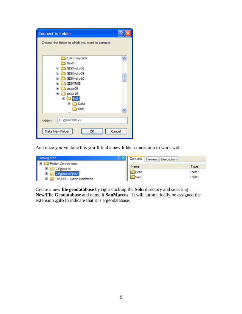
And in the resulting dialog box, connect to the Ex2 folder

9

And once you’ve done this you’ll find a new folder connection to work with:

Create a new file geodatabase by right clicking the Soln directory and selecting

New/File Geodatabase and name it SanMarcos. It will automatically be assigned the

extension .gdb to indicate that it is a geodatabase.

10

Right click on the new SanMarcos geodatabase and select New/Feature Dataset.

Name the new feature dataset Basemap, and hit Next to set the projection and map

extent.

Select Import from the choices in the menu displayed.

11

We will import the coordinate system, so select Import and then navigate to the

NHDPlus data that was just downloaded. Select the nhdflowline shapefile.

Hit Add to select this horizontal coordinate system. Hit Next and leave the Vertical

Coordinate system set at None.

12

Hit Next and leave the default XY Tolerances as they are, then hit Finish to complete

the specification of the spatial reference of the feature dataset. If you right click on the

resulting Basemap feature dataset and open Properties, and tab to XY Coordinate

System, you’ll see the coordinate system is GCS_North_America_1983. This means

that the coordinate system is in geographic coordinates using the North American Datum

of 1983. You’ll learn about the delights of this marvelous coordinate system in our next

class!

What we’ve done in ArcCatalog is to create a receptacle for the datasets for the San

Marcos basin that we are now going to compile.

Displaying Streams and Watersheds

13

Open ArcMap, either by using the same process as you used before to open ArcCatalog

from the Start menu, or directly from within ArcCatalog by hitting the ArcMap symbol

button. Close ArcCatalog since we won’t be using it again for a while.

Hit Cancel on the window within the ArcMap display and

use the button in the ArcMap menu bar to add some data. Use the up arrow

navigate to the Data folder for this purpose.

We will first add the subbasin and flowlines layers. The NHDflowline.shp shapefile is

located in the Hydrography folder and the wbdhu12_a_tx.shp shapefile is located in

HydrologicUnits folder. Please note that in this HydrologicUnits folder I have

substituted the Watershed Boundary Dataset HUC12 watersheds (wbdhu12_a_tx) for the

normal HUC8 watershed files that come with the NHDPlus dataset. NHDPlus is being

updated to include the HUC12 watersheds but that work is not complete yet.

14

You might get a map that shows up as below with arbitrarily selected colors for the

watersheds and streams.

15

To recolor the watersheds (wbdhu12_a_tx), click on their symbol in the Table of

Contents on the left side of the ArcMap display, select a nice green color in the Symbol

Selector, and then click ok!

Similarly, click on the symbol for the streams, and select a nice blue for symbolizing

rivers . Now right click on the wbdhu12_a_tx layer and select Zoom to Layer

16

And you’ll see a nice new map with green watersheds and blue rivers and streams. All is

right in the world!!

You can see the watersheds that are roughly in the outline of Texas and the NHD stream

network that covers Water Resource region 12. As you move the pointer around the map

display you’ll see the location in decimal degrees shown in the lower right hand corner of

17

ArcMap. The map extent of a data set is the combination of two pairs of coordinates, one

on the lower left and the other on the upper right of the map that measure, respectively,

the West, South, East and North extents of the map information.

Use File/Save As to save the ArcMap document as Ex2.mxd (to save your own

customized colors).

To Be Turned In: Screen capture the resulting map display and include it in your

solution. What is the map extent in decimal degrees of these data?

Selecting the Watersheds in the San Marcos Basin

The HUC12 Watershed, and NHDflowlines feature classes cover a large region and we

only want to work in the San Marcos Basin. We'll use ArcMap to identify the San Marcos

SubBasin and to create new feature classes using pertinent portions of the feature classes

for Region 12.

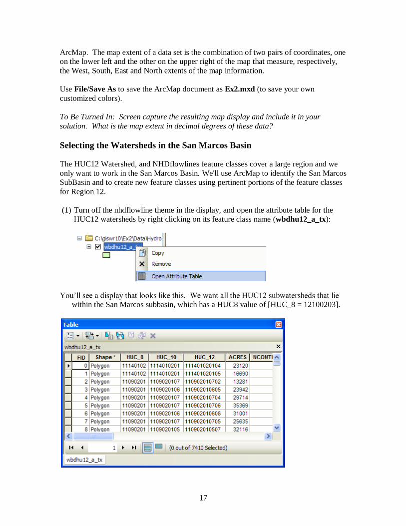
(1) Turn off the nhdflowline theme in the display, and open the attribute table for the

HUC12 watersheds by right clicking on its feature class name (wbdhu12_a_tx):

You’ll see a display that looks like this. We want all the HUC12 subwatersheds that lie

within the San Marcos subbasin, which has a HUC8 value of [HUC_8 = 12100203].

18

At the top left corner of the Table, click on the Select by Attributes tool

Click on “HUC8”, “=”, Get Unique Values and then type 12100203 in the Go To box,

double click on the resulting ‘12100203’ to form the expression

"HUC_8" = '12100203'

In the selection window. Be careful about how you do this since the form of the

expression is important. Click Apply and Close the Select by Attributes window.

Once you’ve executed this query, you’ll see that 32 HUC12 subwatersheds are selected,

and if you hit the “Selected” button at the bottom of the Table, you’ll see the selected

records, and also their highlighted images in the map.

19

If you hit the Zoom to Select button in the table, you can see the selected features up

close. You can use the map navigation tools in the ArcMap toolbar to move you map

around and resize it. Pretty cool!!

20

(2) Make sure that Arc Catalog is closed or the next steps may not work. In ArcMap,

Right Click on the watersheds layer (wbdhu12_a_tx) and select Data/Export Data

to produce a new theme. If you get a message saying you can’t do this, it means that

you haven’t shut down Arc Catalog before trying the data export. Close Arc Catalog

and repeat the export steps if this happens

21

Be sure to navigate to where you established the SanMarcos geodatabase earlier and

don’t just accept the default geodatabase presented to you, which is somewhere deep

in the file system that you may never find again! Browse inside your geodatabase to

the Basemap Feature dataset (you’ll have to change the Save as Type to File and

Personal Geodatabase feature classes first), name this new feature class as

Watershed and save it in the geodatabase as a File and Personal Geodatabase

feature class.

22

You will be prompted to whether add this theme to the Map, click Yes. In ArcMap, Use

Selection/Clear Selected Features to clear the selection you just made.

And then Zoom to Layer to focus in on your selected Watersheds. You can click off the

little check mark by the nhdflowlines layer so that you just see the watersheds displayed.

23

Lets make our basin a bit more interesting. Right click on the Watersheds feature class,

and select Properties/Symbology. Use HUC-10 as the Value Field, hit Add All Values to

give each HUC-10 watershed a different color. Hit Apply to get this color scheme

applied to the map.

24

Lets focus on the Watersheds feature class by turning off the display of the other feature

classes. Click on the little symbol to the left of the feature class name in the Table of

Contents area and make wbdhu12_a_tx and nhdflowline not Not Visible.

And you’ll get this nicely colored map of the watersheds and subwatersheds of the San

Marcos basin.

Notice that the 32 HUC-12 subwatersheds have been grouped into five watersheds within

the San Marcos subbasin (I am here using the Watershed Boundary Set nomenclature to

refer to the drainage area hierarchy in its formal sense).

Highlight the Watershed feature class in the Table of Contents, and go up near the top of

the San Marcos Basin, select the Identify tool, and click on one of the HUC-12

subwatersheds. You’ll see its attributes pop up. Notice how the hierarchy of numbers for

the HUC_8, HUC_10, and HUC_12 attributes.

25

Use File/Save to save your Ex2.mxd map file with the new information that you’ve

created.

Creating a San Marcos Basin Boundary

It is useful to have a single polygon that is the outline of the San Marcos Basin. Click on

the Search button in ArcMap and within the Search box that opens up on the right

hand side of the ArcMap display, click on Tools and then type Dissolve. You will see

the autocomplete tool gives you several options and select dissolve (data management)

26

You’ll see a Dissolve tool window appear. You can drag and drop the Watershed

feature class from the Table of Contents into the Input Features area of this window.

Navigate to the BaseMap feature dataset and type Basin as the name of your Output

Feature Class. Click on HUC_8 as your Dissolve_Field. This means that all

Watersheds with the same HUC8 number (12100203) will be merged together. Hit Ok to

execute the function.

There’ll be no apparent activity for a while and then you’ll see the Basin feature

27

Lets alter the map display to make the Basin layer just an outline. Click on the Symbol

for the Basin layer and select Hollow for the shape, Green for the Outline

Color and 2 for the Outline Width.

And you’ll get a very nice looking map of the San Marcos Basin with its constituent

subdrainage areas.

Click on the Catalog window in ArcMap and navigate to your newly created Basemap

feature dataset. Notice how you’ve now got the Watershed and Basin feature classes

that you’ve just created stored inside it.

28

Resave your ArcMap file Ex2.mxd.

To be turned in: A screen capture of the San Marcos basin with its HUC-10 and HUC-12

watersheds and subwatersheds.

Selecting the San Marcos Flowlines

Click on the symbol to the left of nhdflowline in the Table of Contents to make the

flowlines visible again.

29

Now we can create a layer with just the flowlines in the San Marcos Basin. In ArcMap,

use Select/Select by Location to select the features from nhdflowline as the Target

Layer and Basin as the Source Layer, and use the Spatial Selection Method “Target

layer(s) features are within the Source layer feature”. This selects all the streams in the

San Marcos Basin.

Right click on the nhdflowlines feature class and select Data/Export Data

30

Save the selected features as Flowline in the BaseMap feature dataset and add it as a

layer to the map. Remove the old nhdflowline and wbdhuc12_a_tx themes from your

map display by right clicking on the Layer name and selecting Remove.

Right click on the Watershed feature class and under Properties/Symbology, assign a

Single Symbol for the features and select that Symbol to be Hollow

If necessary, change your symbology so that your flowlines are colored in blue. We want

to have our streams looking liking real map streams!

Now you’ve got a map where you can see your flowlines within the areas they drain.

Very nice!

31

Lets add a basemap to give this data a sense of spatial context.

Choose the Topographic Base Map from the ones offered:

32

Don’t worry about warning messages about changes in coordinate systems that you may

see here.

That looks very cool!! You can see where the San Marcos basin lies in between Austin

and San Antonio.

Save the Ex2.mxd file again.

Now let’s look at some summary statistics of the flowlines. Open the Attribute table

Right click on the LengthKm field and select Statistics

33

From this display, you can see the statistics of the LengthKm of the Flowlines. There are

555 flowlines whose average length is 3.40 km and the total length is 1888 km. You can

do the same query on the Acres attribute of the Watershed feature class to get watershed

areas. (1 acre = 0.0040469 km2).

To be turned in: How many HUC12 subwatersheds are there in the San Marcos Basin?

What is their average area in acres and in km2? What is the total area of this basin in

km2? What is the ratio of the length of the streamlines to the area of the HUC12

subwatersheds (called the drainage density) in km-1

?

Adding Attributes to the Flowlines

Now we will use the flowline attributes table to symbolize the flowlines based on their

mean annual flow. Add the table flowlineattributesflow.dbf to your ArcMap display.

34

Lets zoom into our Flowlines and use the Inquiry button in the Tools menu to see

the attributes of one of them. You’ll see there is a number called the COMID that

uniquely identifies each flowline feature in the NHD. In this case, COMID = 1628231.

This is an arbitrary integer that describes one stream segment in the NHD. You’ll also

see the ReachCode = 12100203000200 in this case. This means that this is segment 200

within HUC8 Subbasin = 12100203. You’ll also see reference here to GNIS, which is

the Geographic Names Information System, the official set of names for things in the

United States. We have systems for everything!

35

If you open the Attributes table of FlowLineAttributesFlow.dbf, you’ll see that it also has

a COMID field and lots of tabular attributes that tell you more about the properties of the

flowline. We’ll use COMID as a key field to link the two attribute tables and transfer

mean annual flow attributes to the Flowline feature class. Just for fun, I’ve use the

“Select by Attributes” tool in the Table to select the record in the

FlowLineAttributesFlow.dbf table that tells us more about this particular stream with

‘COMID’ = 1628231. It has a Mean Annual Flow of (MAFLOWU) of 3.82 cfs, a

corresponding flow velocity of 0.95 ft/s. These are very useful data for water flow

computations.

36

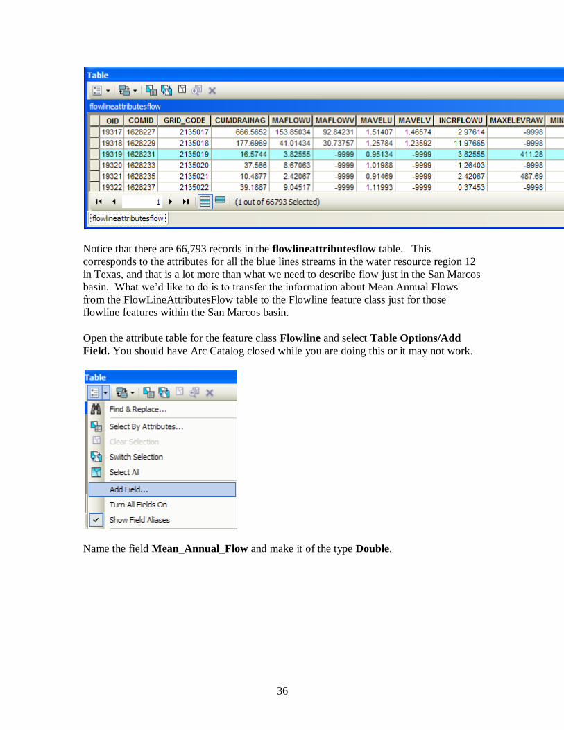
Notice that there are 66,793 records in the flowlineattributesflow table. This

corresponds to the attributes for all the blue lines streams in the water resource region 12

in Texas, and that is a lot more than what we need to describe flow just in the San Marcos

basin. What we’d like to do is to transfer the information about Mean Annual Flows

from the FlowLineAttributesFlow table to the Flowline feature class just for those

flowline features within the San Marcos basin.

Open the attribute table for the feature class Flowline and select Table Options/Add

Field. You should have Arc Catalog closed while you are doing this or it may not work.

Name the field Mean_Annual_Flow and make it of the type Double.

37

This creates a new field at the right hand end of the attributes table that has <null entries>

in it for the moment. Notice that there are 555 features in the flowline feature class.

Now we will join the Flowline layer with the flowlineattributesflow table based on

COMID. Right click on the Flowline layer and select Joins and Relates/Join.

38

Select the COMID field and the flowlineattributesflow table as the one you are going to

join to

Say no to creating an index.

Now when you open the Flowline attribute table, at the right hand end of the table, you

will find the information contained in the flowlineattributesflow table has been joined to

the existing features. Scroll over to the column labeled

flowlineattributesflow.MAFLOWU. This field contains the Mean Annual Flow for each

reach. It is estimated by averaging the mean annual runoff over the drainage area above

this reach. If you look at your COMID’s and several rows look the same, it is because

your display width for the field is not wide enough to display all the integers in the

COMID. Drag the dividing line to the right of the field header COMID to the right and

you’ll see unique COMID values. All is well! Notice that in this joined table, we’ve

only got 555 records with flow values in them, not the 66, 793 values we had earlier.

39

We can set the value of our new field Mean_Annual_Flow by using the field calculator.

Scroll back to the column we created, called Mean_Annual_Flow, and right click on the

column label to select the field calculator.

40

Set this field equal to [flowlineattributesflow.MAFLOWU]. This populates the Mean

Annual Flow field with the appropriate value.

Now we can remove the join by right clicking on the Flowline feature class and selecting

Joins and Relates/Remove All Joins.

Now our attribute table for SanMarcos_flowlines has a field called Mean_Annual_Flow

with the values populated.

41

We can use this field to symbolize the flowlines. Right click on Flowlines and select

properties. In the properties menu, select the Symbology tab. Change the Symbology to

display graduated symbols for the Mean_Annual_Flow field and hit OK. Click on the

Template symbol to change the color of the lines from the arbitrary one selected by the

symbol editor.

The result is a map displaying the relative flow of the streams and rivers in the San

Marcos basin. This is a much more instructive map that shows the main rivers of the

San Marcos basin, the Blanco, San Marcos Rivers along the main steam, and Plum Creek,

a tributary coming in from the North near the downstream end of the basin.

42

Use the Inquiry tool to find out the names of the various rivers in the map display.

Right click in the grey area to the right of the existing toolbars to open the Draw toolbar

and select a label:

And add a label to show Plum Creek:

43

To be turned in: a screen capture of the San Marcos Basin and streams. Add labels to

show the San Marcos River, the Blanco River and Plum Creek.

Resave your Ex2.mxd file.

Creating a Point Feature Class of Stream Gages

Now you are going to build a new Feature Class yourself of stream gage locations in the

San Marcos basin. I have extracted information from the USGS site information at

http://waterdata.usgs.gov/tx/nwis/si

44

(a) Define a table containing an ID and the long, lat coordinates of the gages

The coordinate data is in geographic degrees, minutes, & seconds. These values need to

be converted to digital degrees, so go ahead and perform that computation for the 8 pairs

of longitude and latitude values. This is something that has to be done carefully because

any errors in conversions will result in the stations lying well away from the San Marcos

basin. I suggest that you prepare an Excel table showing the gage longitude and latitude

in degrees, minutes and seconds, convert it to long, lat in decimal degrees using the

formula

Decimal Degrees (DD) = Degrees + Min/60 + Seconds/3600

Remember that West Longitude is negative in decimal degrees. Shown below is a table

that I created. Be sure to format the columns containing the Longitude and Latitude

data in decimal degrees (LongDD and LatDD) so that they explicitly have Number

format with 4 decimal places using Excel format procedures. Format the column

SITEID as Text or it will not retain the leading zero in the SiteID data. Add the

additional information about the USGS SiteID, SiteName and Mean Annual Flow

(MAF). Note the name of the worksheet that you have stored the data in. I have called

mine Latlong. Close Excel before you proceed to ArcMap.

(b) Creating and Projecting a Feature Class of the Gages

(1) Open ArcMap and the Ex2.mxd file you created in the first part of this exercise.

Select the add data button and navigate to your Excel spreadsheet

45

Double click on the spreadsheet to identify the individual worksheet within the

spreadsheet that you want to add to ArcMap (it’s a coincidence that they have the same

name in this example and that is not necessary in general).

Hit Add and your spreadsheet will be added to ArcMap. Pretty cool!! Its always been a

struggle to add data from spreadsheets before and it seems like at ArcGIS 10, they have

gotten this right.

Now we are going to convert the tabular data in the spreadsheet to points in the ArcMap

display.

(2) Right click on the new table, LatLong, and select Display XY Data

46

(3) Set the XY Table to latlong, the X Field to LongDD (or Longitude), the Y Field to

LatDD (or Latitude), Hit Edit to change the spatial coordinate system, and then Import,

and get the coordinate system from the feature dataset Basemap, and you should end up

with a display that looks like the one below. Click on the Show Details button to see

details of the Geographic Coordinate System. We’ll learn about these in our next lecture!

47

Hit OK, to complete it and you’ll get a warning message about your table not having an

ObjectID. Just hit Ok and move on. Hit Ok to add the points and voila! Your gage

points show up on the map right along the San Marcos River just like they should.

Magic. I remember the first time I did this I was really thrilled. This stuff really works.

I can create data points myself! If you don’t see any points, don’t be dismayed. Check

back at your spreadsheet to make sure that the correct X field and Y field have been

selected as the ones that have your data in decimal degrees.

Click on the point symbol under the legend label latlong event and recolor and resize the

points so that they show up more clearly. You’ll see that you have 3 sites on Plum

Creek, 3 sites on the San Marcos River, and two sites on the Blanco River, an upstream

tributary of the San Marcos River.

48

What you have created is called an “event” which means that it is a graphical display in

the ArcMap window of latitude and longitude points that are stored in a table. It is not a

real feature class yet.

Resave your Ex2.mxd file. When I was preparing the exercise, I had a crash in the next

step in ArcMap, so be sure your work is saved at this point!

(4) Now, we’ll make a feature class out of the points. Right click on the latlong

Events layer and select Data/Export Data

49

And export the data into the Basemap feature dataset as the feature class

MonitoringPoint. Say Yes when you are asked if you want to add the points to your

map, and now you’ve got a new feature class in the Basemap feature dataset with your

points in the same projection as the other features in Basemap (ArcGIS does the map

projection automatically as part of the data export process).

Remove the Latlong table and the Latlong Event layers from the ArcMap display and

recolor and resize the MonitoringPoint features so that you can see them easily.

50

Open the attribute Table of the new MonitoringPoint feature class, and you can see on

the right hand side, a new field called Shape that was added when the feature class was

formed. This is where the geographic coordinates of the points are stored in a way that

ArcMap can readily visualize them.

51

In ArcMap, open an ArcCatalog window using the button and expand the contents of

your BaseMap feature dataset. The MonitoringPoint feature class now resides there.

(5) Close the ArcCatalog window and Save your Ex2.mxd ArcMap document.

Labeling the Gages in View

Right click on the MonitoringPoint feature class and select Properties.

52

Click on the Labels tab and from the drop down menu select the label field name to be

SiteName. Change the size of your font to 12 point type.

Right click on the MonitoringPoint feature class again and select Label Features.

53

You can now create a view like this:

Creating a Chart and Layout

(1) Open ArcMap to create a chart of the mean annual flow of the San Marcos gages. The

Mean Annual Flow at the gages is recorded in the column labeled MAF in the

attribute table. Open the MonitoringPoint attributes table and make a chart using the

tools available in ArcMap. Click on the Table Option and select Create Graph

54

Select Graph Type as Horizontal Bar, MAF as the Value Field, GageNo as the X

field, click off the Add to Legend, Select a Custom Color of blue, and hit Next

55

In the next window, change the chart title, Left axis property to leave SITENAME

blank, and Bottom axis property to Mean Annual Flow (cfs)

56

It took me several attempts to get this result but it looks quite nice I think.

In ArcMap prepare a layout showing a map of the drainage area, the graph of its

annual flows at each gage. Move your graph off to one side of your display, and under

View, select Layout View. You’ll see a new window appear and a map pop up in it

57

Resize the map so it doesn’t take up all the page, and then right click on your Chart and

say Add to Layout. Resize the chart so it is comparable in size to the map. Use the

Insert toolbar in ArcMap to add a Title, North Arrow and Scale bar to your Layout.

58

You can right click on the Title to get its Properties and then use Change Symbol to get

a new text size. You can right click on the Scale bar, select Properties and then

Division Units to select the distance units you want. Here is what I got when I did all

this. Pretty cool!

59

You can import Excel chart and worksheet from the Insert/Object... option in

ArcMap. If necessary resize the original chart or table smaller so that it can be displayed

in the layout. You'll see in the chart that the flow in the San Marcos River at Luling and

Ottine is much higher than in the upstream stations. That is because of the cumulative

effect upstream at Luling and because Plum Creek joins the San Marcos River just

upstream of Ottine.

60

Save your Ex2.mxd file.

To be turned in: a layout showing the base map, and chart for the San Marcos River

flows

Overlaying the Edwards Aquifer

The Edwards aquifer is one of the most critical water resources of Central Texas. It is the

main source of water supply for San Antonio, the 10th largest city in the United States.

The Edwards aquifer is recharged by infiltration from rivers crossing its outcrop area. To

determine where the San Marcos River crosses, the outcrop area, I obtained a coverage of

the Edwards aquifer from the Texas Natural Resource Information System

(http://www.tnris.state.tx.us/)

The Edwards aquifer coverage from TNRIS is in Decimal Degree coordinates. This is the

Edwards shapefile that you copied from the zip file at the beginning of the exercise.

Open the ArcCatalog window within ArcMap using the button. Right click on the

Basemap Feature Dataset and select Import/Feature Class (single).

Navigate to the Edwards shape file in the dataset supplied for the Exercise, and name the

Output Feature Class Aquifer.

61

This will not only do the conversion from shapefile to feature class, but also add the new

feature class to your map.

Right click on the Aquifer feature class and select Properties. Click on its Symbology tab

and Label the theme using the attribute Aquifer. This attribute has three values: 1 for

outcrop, 2 for downdip and 0 for holes within the outer boundary of the aquifer. Classify

the values with Unique Value and color them appropriately.

You'll see that as the San Marcos River flows South East towards the Gulf Coast and it

crosses first the outcrop and then the downdip portions of the Edwards aquifer. The

downdip region is where the aquifer dips below the land surface and is shielded from the

surface rivers by overlying hydrogeological units of low permeability. The Edwards is a

62

fissured limestone aquifer whose fissures lie along its Southwest to Northeast orientation,

so its flow moves in that direction, transverse to the direction of flow in the San Marcos

basin. It is thus quite possible for water to drain from the San Marcos river into the

Edwards aquifer and then reappear as a spring further North in another river. Zoom in to

the region where the aquifer crosses the San Marcos basin for a closer look.

To be turned in: Between which two gaging stations does the Edwards aquifer outcrop

area occur? What is the difference in mean annual flow at these two gages? Comment on

these data. Do they seem correct to you?

Summary of Items to be Turned in:

1. Screen capture the resulting map display and include it in your solution. What is the

map extent in decimal degrees of these data?

2. A screen capture of the San Marcos basin with its HUC-10 and HUC-12 watersheds

and subwatersheds.

3. How many HUC12 subwatersheds are there in the San Marcos Basin? What is their

average area in km2? What is the total area of HUC12 subwatersheds in this basin in

km2? What is the ratio of the length of the streamlines to the area of the HUC12

subwatersheds (called the drainage density) in km-1

?

4. A screen caputre of the San Marcos Basin and streams. Add labels to show the San

Marcos River, the Blanco River and Plum Creek.

5. A layout showing the base map, and chart for the San Marcos River flows.

6. Between which two gaging stations does the Edwards aquifer outcrop area occur?

What is the difference in mean annual flow at these two gages? Comment on these data.

Do they seem correct to you?