Exercise 1

MEASUREMENT OF VIBRATION PARAMETERS

1. Aim of the experiment

Analysis of the methods of measurement of mechanical vibration parameters and the measurement

apparatus.

2. Theoretical introduction

Mechanical vibrations are such a kind of motion, where a body (mass) moves between two extreme

edges crossing the equilibrium position. The vibrations appearing in machines and other technical

devices are an effect of driving forces, e.g., the pressure of combustion gases on the piston, or resistance

forces, and also impacts or changes of the load and external conditions. Apart from forced vibrations

connected with motion of machines, there can also occur self-excited vibrations, which appear, e.g.,

during the operation of cutting tools.

Excessive vibrations cause faster wear of machines, material fatigue, noise, and they exert a

hazardous influence on people. Such vibrations are often a symptom of the machine failure.

Practical applications of vibrations are, for instance, shakers, pneumatic drills, exciters for the

investigations of durability and modal analysis, pattern sources of vibrations for the sensor calibration.

2.1. Measurement of vibrations

The aims of the measurement of vibrations are as follows:

• to control if amplitudes of vibrations of a given frequency do not exceed permissible values,

• to identify the reasons of excessive vibrations in given parts of the machine,

• to isolate or to damp vibrations,

• to monitor the dynamical state of machines,

• to acquire the experimental data for the numerical verification of models of structures.

During the measurement of oscillations, we usually record values of the displacement x, the velocity v

and the acceleration a as a function of time. Among these data, the following relationship holds:

dt

dxv = ;

2

2

dt

xd

dt

dva == . (1.1)

Theoretically, it is enough to measure one of the above values, and the remaining variables can be

calculated as an integral or a time derivative. In the case of harmonic vibrations with the frequency ω,

the displacement, the velocity and the acceleration are given as:

txx ωcos0= ; txv ωω sin0−= ; txa ωω cos0

2−= . (1.2)

The above-mentioned calculations can be easily made analytically. These calculations can be carried out

directly during the measurement by means of electrical systems for integration or differentiation of the

signal. Thus, it seems to be no matter which variable characterizing the oscillations will be directly

measured. However, it is not quite right, because experimental electrical integration or differentiation

processes decrease the accuracy of the amplitude calculation and cause some phase shift between the

measured and output signal. Therefore, we should take care to which mechanical quantity the electrical

signal, obtained from the sensor, is proportional during electrical measurements of mechanical quantities.

z2 z1 z2

x

UG

+x

E1 E2

z1

Uout=E1-E2

z2 z2

-x

Core

The most often used sensors in the measurement of mechanical vibrations are:

• inductive transformer sensors, which give the signal proportional to the displacement,

• electro-dynamic sensors, delivering the signal proportional to the velocity,

• seismic, piezoelectric sensors giving the signal proportional to the acceleration value.

2.1.1. Measurement of vibrations with difference transformer sensors

In transformer sensors with variable mutual inductance, the dependence of the electromotive force

(induced from the primary coil winding to the secondary coil winding) on the mutual inductance

coefficient is used in measurements. The sensor shown in Fig. 1.1 has one primary winding z1 and two

secondary windings z2 (of the same number of coils) coiled round a cylindrical isolating sleeve. The

windings are connected against each other (a push-pull system). A ferromagnetic core moves inside the

sleeve. This core is connected through the pivot with a vibrating object. The primary winding is supplied

with sinusoidal voltage of the frequency varying from 5 Hz to 50 Hz.

Fig. 1.1. Inductive transformer sensor

The electromagnetic force induced in the secondary coils is equal to:

dt

dze

Φ−= 22 . (1.3)

The part Φ0 of the magnetic flux Φ, which is generated by the primary coil winding of z1 coils, is

associated with the coils z2 of both secondary windings. The part Φ’ of this flux is associated with the

upper coil winding, whereas the part Φ’’ is associated with the lower coil winding. In these coil windings

of z2 coils, the electromotive forces arise:

)'( 021 Φ+Φ= zE ω ; )''( 022 Φ+Φ= zE ω . (1.4)

In the case of the central position of the core, we have Φ’ = Φ’’ = Φ1. Since the windings are push-

pull connected, thus we have Uout = E1 - E2 = 0. The displacement of the core, e.g., upwards, causes an

increase ∆Φ of the magnetic flux Φ’, penetrating the upper coil winding. Simultaneously, the magnetic

flux Φ’’, penetrating the lower coil winding, decreases by a value ∆Φ, thus we have:

Φ’ = Φ1 + ∆Φ, and Φ’’ = Φ1 – ∆Φ.

The sensor output voltage Uout is equal to:

1 2 22outU E E zω= − = ∆Φ . (1.5)

The change of the magnetic flux is as follows:

1 11

1 2 1 2

RIz IzIz

R R R R

µ

µ µ µ µ

∆∆Φ = − = , (1.6)

where:

∆Rµ – change of magnetic resistances of the windings Rµ2 and Rµ1, caused by a displacement of the core

from the central position x,

I – current in the primary winding; ω – pulsation of the current I, (ω=2πf , f – frequency of the current supplying the winding).

The change of the magnetic resistance (reluctance) ∆Rµ is proportional to the core displacement x:

0

1 2

Rk x

R R

µ

µ µ

∆= . (1.7)

Finally, we obtain:

0 1 22outU k z z Ix kxω= = . (1.8)

Inductive differential sensors are characterised by high precision and sensitivity, because they can

have a large number of coils in their winding.

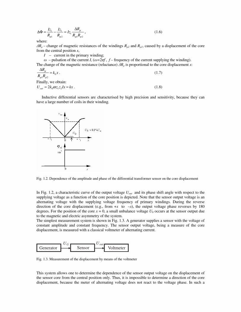
Fig. 1.2. Dependence of the amplitude and phase of the differential transformer sensor on the core displacement

In Fig. 1.2, a characteristic curve of the output voltage Uout and its phase shift angle with respect to the

supplying voltage as a function of the core position is depicted. Note that the sensor output voltage is an

alternating voltage with the supplying voltage frequency of primary windings. During the reverse

direction of the core displacement (e.g., from +x to –x), the output voltage phase reverses by 180

degrees. For the position of the core x = 0, a small unbalance voltage U0 occurs at the sensor output due

to the magnetic and electric asymmetry of the system.

The simplest measurement system is shown in Fig. 1.3. A generator supplies a sensor with the voltage of

constant amplitude and constant frequency. The sensor output voltage, being a measure of the core

displacement, is measured with a classical voltmeter of alternating current.

Generator Sensor VoltmeterUoutUG

Fig. 1.3. Measurement of the displacement by means of the voltmeter

This system allows one to determine the dependence of the sensor output voltage on the displacement of

the sensor core from the central position only. Thus, it is impossible to determine a direction of the core

displacement, because the meter of alternating voltage does not react to the voltage phase. In such a

system, for unequivocal measurement of the displacement, we can employ a half of the sensor

measurement range – one of the branches of the characteristic curve (see Fig. 1.2).

UG

UG

U1 U2 U

x

Uout

W DF FD

G

Fig. 1.4. Block scheme of the sensor with phase-sensitive rectification

0

Measurement range

of the sensor

x

U

∆x

∆U

Transformer sensors usually work in the system shown schematically in Fig. 1.4. The generator G

supplies the sensor and the phase-sensitive rectifier DF with the voltage of constant amplitude and

frequency. The amplifier W is designed to amplify the output voltage Uout from the sensor. In the phase-

sensitive rectifier DF, the voltage from the amplifier is rectified, taking into account the phase of this

voltage with respect to the voltage UG from the generator. This voltage assumes positive and negative

values, depending on the direction of the sensor core displacement from the central position, but it

contains unwanted “pulsations” of the generator voltage frequency. The low-pass filter FD “lets through”

only the signals of low (in comparison with the frequency of the generator) frequencies. In the signal

from the rectifier, there exists a low frequency of the envelope of the core displacement signal. For

proper mapping of the core motion, the frequency of the generator should be several times higher than

the frequency of measured vibrations.

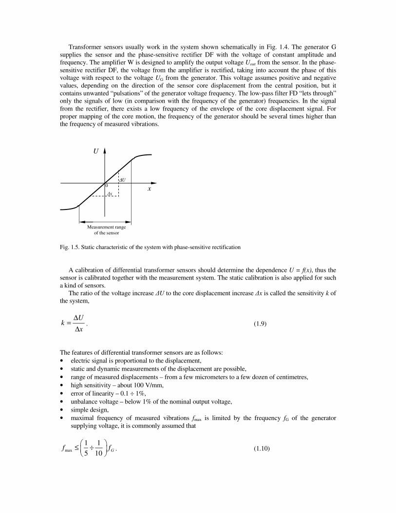
Fig. 1.5. Static characteristic of the system with phase-sensitive rectification

A calibration of differential transformer sensors should determine the dependence U = f(x), thus the

sensor is calibrated together with the measurement system. The static calibration is also applied for such

a kind of sensors.

The ratio of the voltage increase ∆U to the core displacement increase ∆x is called the sensitivity k of

the system,

x

Uk

∆

∆= . (1.9)

The features of differential transformer sensors are as follows:

• electric signal is proportional to the displacement,

• static and dynamic measurements of the displacement are possible,

• range of measured displacements – from a few micrometers to a few dozen of centimetres,

• high sensitivity – about 100 V/mm,

• error of linearity – 0.1 ÷ 1%,

• unbalance voltage – below 1% of the nominal output voltage,

• simple design,

• maximal frequency of measured vibrations fmax is limited by the frequency fG of the generator

supplying voltage, it is commonly assumed that

max

1 1

5 10Gf f

≤ ÷

. (1.10)

The movable mandrel, connected with the sensor core, comes in contact with the vibrating object.

Thus, object vibrations with respect to the reference system, where the housing of the sensor is fixed,

are measured. Under real conditions of the vibration measurement, it is difficult to obtain an

unmovable reference system, which limits applications of these sensors.

2.1.2. Measurement of vibrations with electro-dynamic sensors

The operating principle of electromagnetic sensors comes from the electromotive force E induced

in the winding moving in the field of the permanent magnet:

BlvE = , (1.11)

where:

B – induction generated by the permanent magnet,

l – winding length (depends on the number of coils),

v – velocity of the winding in the magnetic field (relative velocity of the coil winding and the

magnet).

By means of electro-dynamic sensors, the velocity of vibrations can be measured directly. These

sensors are the so-called generating sensors, i.e., they do not require a power supply, and they generate

the electromotive force themselves.

Usually, the coil winding in electro-dynamic sensors moves with respect to the magnet, but there

are also solutions with a movable magnet. In both cases, the electromotive force is proportional to the

relative velocity of the coil winding and the magnet.

Electro-dynamic sensors are designed to measure relative vibrations and absolute vibrations

(seismic). The seismic sensor is a one-degree-of-freedom system possessing a seismic mass m, a

spring of the rate k and a viscous damper of the damping coefficient c. The housing of such a sensor is

fixed to the vibrating object (Fig. 1.6). The equation of motion of the mass m can be formulated from

the d’Alembert principle:

( ) ( ) 0mx c x y k x y+ − + − =&& & & . (1.12)

Fig. 1.6. Design and model of the mechanical system of the seismic electro-dynamic sensor

The output (measured) signal usually depends on the relative motion z(t) (Fig.1.6b) of the mass and

the housing:

b)

z(t)

k

m

c

x(t)

y(t)

Object under analysis

a)

E=Blv

winding

magnet

spring

)()()( tytxtz −= (1.13)

where:

x(t) – coordinate describing the mass motion with respect to the unmovable coordinate system (with

respect to the Earth),

y(t) – coordinate describing the sensor housing motion, i.e., the motion of the object under

investigation.

Hence, equation of motion (1.12) can be rewritten as:

mz cz kz my+ + = − &&&& & , (1.14)

or in the form:

yzzhz &&&&& −=++ 22 α , (1.15)

where:

m

k=α – angular natural frequency of vibrations,

m

ch

2= – coefficient of viscous damping related to the mass,

α

εh

= – dimensionless coefficient of damping. (1.16)

If the excitation of vibrations has the harmonic character described by the function y=y0 sinωt, then

the solution to Eq. (1.15) consists of two components: the transient one with the frequency of damped

vibrations 22

h−= αλ , disappearing with velocity and depending on the damping coefficient ε, and

the second component representing steady-state vibrations:

)sin(0 ϕω −= tzz . (1.17)

The amplitude z0 and the phase of relative vibrations (phase shift angle) are determined by the

relations:

2222

2

00

)2()( ωωα

ω

hyz

+−= ;

22

2

ωα

ωϕ

−=

harctg . (1.18)

The sensitivity k of the transducer is defined by the amplitude ratio, according to the formula:

2222

2

0

0

)2()( ωωα

ω

hy

zk

+−== . (1.19)

The diagram of the amplitude ratio (Eq. (1.19)) as a function of the forcing frequency (or the ratio

ω/α) has multiple applications, because:

a) characteristics of the sensor are identical, regardless of the fact if we consider the amplitudes of

displacement, velocity or acceleration, as:

2

0

2

0

0

0

0

0

ω

ω

ω

ω

y

z

y

z

y

z== , (1.20)

where: z0 , z0ω, z0ω2 – amplitudes of displacement, velocity and acceleration of the coil winding

vibration with respect to the magnet (the housing),

y0, y0ω, y0ω2 – amplitudes of displacement, velocity and acceleration of the housing vibration,

0

30

60

90

120

150

180

0 1 2 3 4 5 6 7 8ω/ αω/ αω/ αω/ α

ϕϕϕϕ absolute vibrations

relative vibrations ε=0,6

ε=0,2

ε=0,2

0

1

2

3

4

0 1 2 3 4 5 6 7 8ω/αω/αω/αω/α

k, k 1

relative vibrations

absolute vibrations

ε=0,2

ε=0,6

ε=0,2

b) characteristics allow us to correct quickly the measurement error, introduced by the sensor, in

dimensionless units or in %.

For the absolute motion x of the mass m, the transfer coefficient 1 0 0k x y= and phase shift angle ϕ

are defined by the following relations:

2222

24

0

01

)2()(

)2(

ωωα

ωα

h

h

y

xk

+−

+== ;

22

2

ωα

ωϕ

−

−=

harctg . (1.21)

Fig. 1.7. Frequency, amplitude and phase characteristics of the seismic sensor

The sensor does not introduce an error only in the case of z0/y0 = 1 (Fig. 1.7). In fact, it takes place when

the frequency of measured vibrations ω is at least three times higher than the natural frequency α. Then,

the seismic mass is practically unmovable with respect to the ground. We can obtain a larger range of the

flat amplitude characteristic curve by an appropriate selection of damping. The most proper is the

coefficient of damping ε = h/α ≈ 0.6. Taking under consideration a correction of the amplitude and a

correction of the phase shift angle, we can extend the sensor measurement range to the region of

frequencies even lower than the natural frequency α.

The sensor should give a non-deformed view of measured vibrations, i.e., deformations of the

amplitude and phase should not occur. The main reason of non-linear deformations of complex time

histories of vibrations (containing different frequencies) is a phase shift. For example, the analysed

signal

(Fig. 1.8) contains the second harmonic, which is reconstructed by the sensor with a different phase

shift than the first one, which introduces a non-linear deformation of the signal.

-1,5 0U -1

-0,5

0

0,5

1

1,5

2

-1 0 1 2 3 4 5 6 7 8 t

v

t 1 = φ 1 / ω 1

t 2 = φ 2 / ω 2

2nd harmonic1st harmonic

Fig. 1.8. Influence of the phase shift in the electro-dynamic sensor on non-linear deformations

The features of seismic electro-dynamic sensors:

• electric signal is proportional to the velocity of vibrations, thus dynamic calibration is required

for them,

• they do not require the reference system (they are mounted directly on the object),

• they do not require the power supply,

• they have a simple design,

• it is possible to obtain high sensitivity by increasing the number of winding coils,

• small coil winding resistance (about 10 kΩ), which enables operation with an arbitrary voltmeter

device,

• large size, relatively large mass (about 0.5 kg),

• necessity of determining the frequency of measured vibrations in order to consider a correction of

sensor indications,

• in typical sensors, the natural frequency is 10 ÷ 20 Hz.

The electrical damping is performed by means of eddy (Foucault) currents. They are induced

during the motion in a copper cylinder which is located in the same air gap. The additional correction

winding makes a change of the damping coefficient (in order to compensate the temperature influence)

possible and enables the compensation of static deflection of springs during the vibration measurement

along the vertical direction.

Fig. 1.9. Seismic electro-dynamic sensor, type PR9266: 1 – permanent magnet,

2 – measurement coil winding, 3 – damping winding, 4 – correction winding,

5 – membrane spring, 6 – stop, 7 – housing, 8 – shielding cable

5 7 3 1 5 9

6 8 4 2 6

-1,5

-1

-0,5

0

0,5

1

1,5

-1 0 1 2 3 4 5 6 7 8 t

v 1st harmonic

2nd harmonic

The basic technical data of the sensor type PR9266 (Fig. 1.9):

• size: diameter – about 58 mm, height – 101 mm;

• mass – 490 g;

• mass of the movable system of the sensor – 21 g;

• resonance frequency (without damping) along the horizontal direction – about 12 Hz;

• frequency range of the measurement – 10 ÷ 1000 Hz;

• damping coefficient – about 0.6;

• nominal sensitivity – 30 mV/mm⋅s-1;

• resistance of the measurement coil winding – 2100 Ω.

2.1.3. Electro-dynamic sensor of relative vibrations

In relative vibration sensors, the mandrel of the movable system (it is usually the coil winding) is in

contact with the vibrating object under investigation. The housing of the sensor has to be mounted in

the reference system, which is usually unmovable, and then vibrations of the object with respect to the

reference system are measured.

Fig. 1.10. Electro-dynamic

sensor, type PR9267

(Philips):

1 – permanent magnet, 2 –

measurement coil winding,

3 – housing, 4 –

membranes,

5 – rubber ring, 6 –

connecting cable, 7 –

spring, 8 – stops, 9 –

springs connection,

10 – tightener, 11 – rubber

rings, 12 – tightener, 13 –

nut, 14 – movable mandrel

The basic technical data of the sensor type PR9267 (Fig. 1.10):

• frequency range of the measurement – 0 ÷ 1000 Hz;

• maximal amplitude of measured vibrations – ± 1mm, short time – ± 2 mm;

• maximal acceleration of measured vibrations – 10 g (98.1 m/s-2

);

• minimal velocity of measured vibrations – 0.05 mm/s;

• nominal sensitivity – 30 mV/mm s-1

;

• mass – 580 g;

• mass of the movable system of the sensor – 37 g.

Some examples of the vibration measurement with the relative vibration sensor are shown in Fig.

1.11. If the frequency of the reference system vibrations is low in comparison with the frequency of

measured vibrations, then an error resulting from the motion of the housing can be small. In such a

case, the sensor can be kept, for instance, in hand.

14 13 12 11 10 9 4 8 8 4

7 5 1 2 3 5 6

Fig. 1.11. Examples of applications of the electro-dynamic sensor of relative vibrations

2.1.4. Measurement of vibrations with piezoelectric sensors

The principle of operation of piezoelectric sensors is based on the piezoelectric effect, which is

typical of some kinds of crystals, e.g. quartz (SiO2). This effect was discovered by the Curie brothers in

1880 and it consists in the appearance of electric charges on crystal faces deformed by the mechanical

load.

Fig. 1.12. Piezoelectric effect in the quartz Fig. 1.13. Piezoelectric effects:

crystal grid longitudinal, transversal and shearing

Electric charges arise in the piezoelectric material subject to compression, bending and shearing stresses.

Piezoelectric sensors are applied in the measurement of forces, accelerations and pressures.

The sensor shown in Fig.1.14 consists of two plates made of a piezoelectric material, on which the mass

m is located. This mass is subject to the pressure from a spring of the rate k in order to ensure the

constant inertia force F = ma during the measurement. Thin metal electrodes (usually made of gold) are

designed for collecting electric charges from faces of the piezoelectric element. The stiffness of the

housing is much higher than the stiffness of the spring, thus it has no influence on the sensor operation.

a) b) c)

Fig. 1.14. Piezoelectric acceleration sensor: a) scheme, b) equivalent mechanical model,

c) equivalent electrical model

+ + + + +

- - - - - + + + +

- - - - + + + + +

- - - - -

q ~ a + C R

Uout

_

Piezoelectric base

mass

seismic mass

mass of the base

k1

k2

k3

piezoelectric

plates

ms

mp

ms

mp

k

Force Force

xa

yak =

][Hzf

If the inertia force, e.g., caused by vibrations, acts on the sensor, then the electric charge q,

proportional to this force, arises on piezoelectric faces and it is a measure of the acceleration, according

to the formula:

kmakFq == . (1.22)

The piezoelectric sensor generates a signal if a variation in the load appears. The piezoelectric

acceleration sensor, whose design and equivalent model is shown in Fig. 1.14, can be treated as a one-

degree-of-freedom spring-mass system with weak damping. This system can be described by the second

order differential equation having the following solution:

2222

24

1

)2()(

)2(

ωωα

ωα

h

h

a

ak

x

y

+−

+== , (1.23)

where:

ay – acceleration of the seismic mass,

ax – acceleration of the sensor housing (measured acceleration),

ω – angular frequency of measured vibrations,

α – natural frequency of vibrations of the spring-mass system.

During a sudden pitch in the excitation, a capacity discharge occurs in the RC circuit due to the internal

resistance R of the sensor. Such a discharge has an exponential character with the time-constant T = RC

(Fig. 1.16a), according to the formula:

RC

t

eQq−

⋅= (1.24)

Fig. 1.15. Characteristic curve of the piezoelectric sensor

In Fig. 1.16b, a response (output signal) to the rectangular excitation is shown.

Fig. 1.16. a) discharge

curve, b) response to the

rectangular excitation

For piezoelectric sensors made of quartz, the time-constant of the sensor intrinsic discharge is very

large, i.e., 102÷10

4 s, because the resistance of quartz is about 10

12 Ω and the capacity about 10

-12 F. It

allows one to measure quasi-static vibrations of the frequency 10-2

Hz, which gives a wide application

range of piezoelectric sensors. Their employment in the full range of frequencies depends on the input

resistance of the measurement apparatus. The addition of the apparatus input resistance causes a change

of the sensor time-constant.

Fig. 1.17. Piezoelectric sensor charcteristic

In practice, the upper range of the measured frequency of vibrations amounts to 0.3 ÷ 0.5 × of the

resonance frequency – then the error does not exceed 12%. For the frequency f = 0.3 × of the resonance

frequency, the error is about 10%

(Fig. 1.17) and the lower frequency range is limited by electric parameters of the sensor and devices

directly connected to it.

If the sensors have large internal capacity, then they can be connected directly to the measurement

system (an oscilloscope, an analyser) characterised by high input impedance (> 1MΩ). Usually this

capacity is small (10-12

F). In order to measure a signal coming from the sensor without deteriorating its

properties, amplifiers are applied.

There are two basic types of piezoelectric transducers, namely:

1) with a charge output – characterised by high output impedance of the piezoelectric element; they

usually require an external charge or a voltage amplifier for further use of the signal,

2) with an internal amplifier – with a built-in self-contained system supplied externally. They are

characterised by low output impedance. Each manufacturer gives them their own name, e.g.

PIEZOTRON® (Kiestler), ICP

® – Integrated Circuit Piezoelectric (PCB Piezotronics),

DELTATRON® (Brüel & Kjær), ISOTRON

® (Endevco)

In Fig. 1.18, a scheme of the measurement system: sensor – cable – voltage amplifier (or other devices of

high output impedance) is shown. High resistance between the mass and the signal (>1012

Ω) has been

assumed. For the opened (unloaded) system, the output voltage of the transducer is given by the relation:

0

1

0 1 2 3 4 5

RCtQeq

/−=

q

t / T

a)

t

t

∆V

1% ∆V

t0 t0+0,01RC

0

b)

useful range

0,3 fr fr

< 10% < 10%

1

1C

qU = , (1.25)

where: q – electric charge [pC], C1 – internal capacity of the sensor (crystal) [pF].

Fig. 1.18. Scheme of the system: a) with a voltage amplifier, b) with a charge amplifier

The voltage, which is measured by the instrument, depends on the capacity of the cable and the input

capacity of the system connected with the sensor:

321

2CCC

qU

++= , (1.26)

where: C2 – capacity of the cable [pF], and, C3 – input capacity of the amplifier or the measuring

instrument [pF].

The dependence of the system voltage sensitivity on the total capacity is seriously limited by the

length of the connecting cable. Such a cable has to be dry and clean as well. In case of measurements in

wet conditions, the connections of the cable to the sensor and the measuring instrument should be sealed.

In the charge amplifier (Fig. 1.18b), the capacitor Cf is located in the feedback circuit. The resistance

of insulation (between the signal and the mass) is large (>1012 Ω) and it is not shown in Fig. 1.18b. The

amplifier output voltage amounts to:

)1(321

2−−++

=ACCCC

qAU

f

(1.27)

where: A – voltage gain of the amplifier with the opened feedback loop.

Since A is very large (about 105), so we have Cf(A-1)>>(C1+C2+C3). The output voltage depends on

the ratio of the charge and the capacity Cf of the feedback capacitor only, thus an influence of the cable

capacity can be neglected.

fC

qU −≈2 (1.28)

In charge amplifiers, there are some limits as far as the cable length is concerned, because the noise

on the amplifier output depends directly on the ratio of the total system capacity (C1 + C2 + C3) and the

feedback capacity Cf. Additionally, due to high impedance of the piezoelectric sensor, special cables of a

U2 U1

C1 C2 C3 C1 C3

U2

Piezoelectric el.

Charging type sensor

cable

Charging amplifier

cable

Piezoelectric el.

Charging type

sensor

Output of the amplifier or the

reading instrument

q

+

C

A

q

+

C2

a) b)

low level of noise are required in order to limit charge variations during the motion (e.g., under bending,

compression or tension) and to reduce the noise caused by electromagnetic disturbances.

Fig. 1.19. Badly and well fixed cable

The system shown in Fig. 1.20 consists of an IEPE type sensor, supplied with voltage from 18V to

30V, a circuit for direct current feeding and a decoupling capacitor (that cuts off a constant component of

the polarization voltage). We obtain an output signal for the measurement or the analysis.

IEPE type sensor

cable

18÷30V

Direct

current

source

Decoupling

capacitor

C

signal

mass

Fig. 1.20. Example of the slotted section of the sensor with integrated electronics

The features of piezoelectric sensors with integrated electronics are as follows:

• they do not require any special cables – a typical double conductor or a concentric cable is good

enough,

• constant sensitivity, independent of the cable length,

• supply from the current source allows us to apply the same double conductor cable also for

sending the signal from the sensor,

• low output impedance – below 100 Ω,

• compact design,

• lower cost of the measurement in comparison with an external amplifier,

• limited range of temperatures (<1250C for typical structures, < 150

0C for special structures).

At present, piezoelectric acceleration sensors are most often applied in vibration measurements due to

their numerous advantages. Since they have no movable parts, they are durable. They are relatively

cheap, reliable in use and easy to calibrate. Such sensors can operate in a wide range of frequencies.

They can be mounted along an arbitrary direction and they allow us to measure vibrations of small

objects due to their small size and mass.

In most sensors produced currently, the piezoelectric shearing effect is employed, e.g. type Shear®

(PCB), or Planar Shear, DeltaShear®, ThetaShear

(Brüel & Kjær). In Fig. 1.21, some examples of these

design solutions are presented.

bad well

Adhesive tape

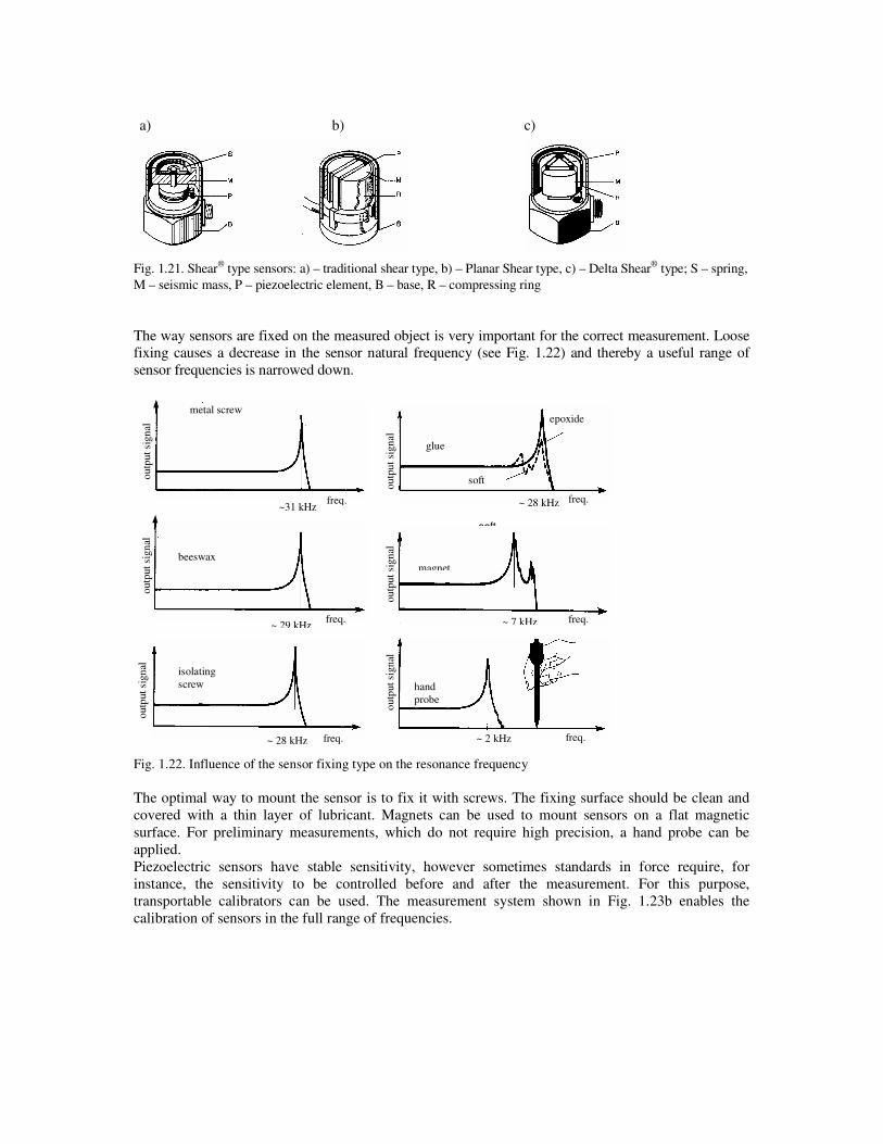
Fig. 1.21. Shear® type sensors: a) – traditional shear type, b) – Planar Shear type, c) – Delta Shear

® type; S – spring,

M – seismic mass, P – piezoelectric element, B – base, R – compressing ring

The way sensors are fixed on the measured object is very important for the correct measurement. Loose

fixing causes a decrease in the sensor natural frequency (see Fig. 1.22) and thereby a useful range of

sensor frequencies is narrowed down.

Fig. 1.22. Influence of the sensor fixing type on the resonance frequency

The optimal way to mount the sensor is to fix it with screws. The fixing surface should be clean and

covered with a thin layer of lubricant. Magnets can be used to mount sensors on a flat magnetic

surface. For preliminary measurements, which do not require high precision, a hand probe can be

applied.

Piezoelectric sensors have stable sensitivity, however sometimes standards in force require, for

instance, the sensitivity to be controlled before and after the measurement. For this purpose,

transportable calibrators can be used. The measurement system shown in Fig. 1.23b enables the

calibration of sensors in the full range of frequencies.

a) b) c)

klej

soft

epoxide

~ 7 kHz

magnet

~31 kHz

~ 2 kHz

hand

probe

outp

ut

sign

al

outp

ut

sign

al

outp

ut

sign

al

outp

ut

sign

al

outp

ut

sign

al

outp

ut

sign

al

freq.

freq.

freq.

freq.

freq.

freq.

~ 28 kHz

~ 28 kHz

~ 29 kHz

beeswax

isolating

screw

glue

epoxide

soft

metal screw

Fig. 1.23. Test

of the sensor

sensitivity: a)

with a

transportable

calibrator, b) by

determining the

frequency

characteristics

with a

calibrating

exciter

(Brüel&Kjær)

Some

modern piezoelectric transducers are available with the TEDS (Transducer Electronic Data Sheet)

function implemented. The built-in memory system in the transducer contains the information about

the transducer – its name tag, sensitivity and the expiration date of the calibrating data. In the

measurement system, the detection of data and their introduction into the system take place

automatically.

3. Measurement devices

During the measurements, the following instruments are used:

1. displacement measurement: a micrometer screw, a differential transformer inductive sensor with a

measuring instrument, a voltmeter, an oscilloscope.

2. velocity measurement: a seismic electro-dynamic sensor with a vibration measuring instrument, an

oscilloscope.

3. acceleration measurement: a seismic piezoelectric sensor with a vibration measuring instrument, a

table for calibrating sensors, an oscilloscope.

The lab test consists in the measurement of vibration parameters of various objects. Before the

measurements, the calibration of sensors and the measurement system should be carried out.

4. Experiment

During the experiment, students are to perform the measurements of vibrations of the object indicated.

For this purpose, students should:

a) select an appropriate sensor,

b) draw a table of measurements,

c) carry out the calibration of the sensor,

d) conduct the measurements of vibration parameters (amplitude and frequency),

e) consider a correction for the electro-dynamic sensor.

5. Report

The report on the experiment should contain:

1) Scheme of the measurement system.

2) Table with the measurement results for the object investigation.

3) Conclusions.

References

amplifier

analyser

tested sensor

calibrating sensor

exciter

a) b)

1. Parszewski Z.: Dynamika i drgania maszyn, WNT, Warszawa 1992.

2. Hagel R., Zakrzewski J.: Miernictwo dynamiczne, WNT, Warszawa 1984.

3. Szumielewicz B., Słomski B., Styburski W.: Pomiary elektroniczne w technice, WNT, Warszawa

1982.

4. Cempel C.: Podstawy wibroakustycznej diagnostyki maszyn, WNT, Warszawa 1982.

5. Engel Z.: Ochrona środowiska przed drganiami i hałasem, PWN, Warszawa 1993.

6. Catalogues of the Philips Company.

7. Catalogues of the Brüel & Kjær Company.