Executive Summary of Biomagnification Teaching and Learning Unit You are what you eat but don’t excrete: Graphing toxic biomagnification

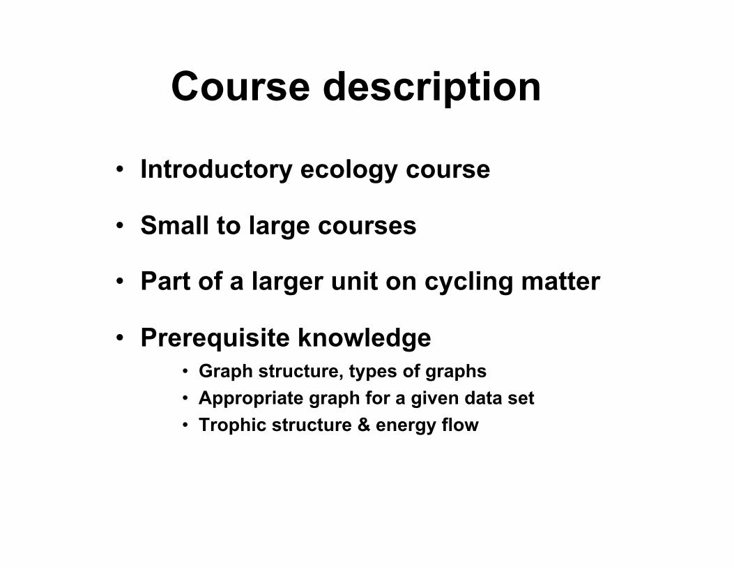
Contributors: Jon Akin, Terry Davin, Win Everham, Evelyn Gaiser, Amanda McConney (facilitator), Courtney Richmond Course description: This unit is intended for a 100- or 200-level introductory general ecology course and is designed to be part of a larger unit on cycling matter. The unit activities could be used for higher level courses with the use of the additional background information. The activities are suitable for small to large class sizes and should take a little more than two 50 minute class meetings. Students’ prerequisite knowledge should include a general understanding of trophic structure and energy flow, graph structure, different types of graphs, and selecting the appropriate graph for a given data set. Learning goals/objectives: By the end of this unit, students will be able to:

• Interpret graphs and draw conclusions from them • Describe the process of biomagnification • Analyze graphs to identify factors that influence the process of biomagnification • Apply the law of conservation of matter to biomagnification

Rationale for Instructional Approach: Our intention was to develop a unity that fostered critical thinking, understanding of the scientific process, and enhanced the students’ abilities to be critical consumers of scientific information. One skill associated with these goals is the ability to interpret graphs. We choose to imbed this skill within a unit on biomagnification, and to use this context to illustrate the complexity of ecological systems. Brief Description of the TL Unit: In this TL Unit, students learn to interpret graphs based on real world data. After a brief Pretest and review of Pretest concepts to identify prior knowledge of graphs and biomagnification, students complete a Think-Pair-Share activity to analyze a complex graph containing actual data. A Minute Paper assessment of the Think-Pair-Share activity provides the opportunity for students to analyze a second graph with different data but the same conceptual framework. Students then complete a two-stage Jigsaw which will further develop their ability to interpret graphs. The first stage consists of students in groups of three, where each student is a unique expert on one of three topics. The three topics deal with factors that influence biomagnification (Physiological factors, Community factors, and Landscape factors). Each expert student will teach their peers about that topic. The groups are then given a Case Study to analyze in Stage 2, with the goal of answering questions and coming to consensus for a report back to the whole class. As a wrap up, the instructor facilitates a review engaging all groups in the discussion of the common trends among the Case Studies, the factors that affect biomagnification, and the concept of persistence in the environment. Assessments include a Pretest, a Minute Paper from the Think-Pair-Share activity, Extended Response Case Study Questions, and Posttest exam questions. How does the TL Unit address active learning? In this unit, the student is actively engaged in learning during the majority of instruction. Students are engaged in a Think-Pair-Share using a graph to introduce the concept of complexity in real world systems. As experts in the Jigsaw, the students teach their peers and answer questions based on an analysis of Case Study graphs.

Biomagnification Teaching and Learning Unit You are what you eat but don’t excrete: Graphing toxic biomagnification

Course level and size: This unit could be taught in a 100 or 200 level introductory general ecology course and is designed to be part of a larger unit on cycling matter. The unit activities could be used for higher level courses with the use of the additional background information. The activities can be used in a small or large class. Authors: Jon Akin, Terry Davin, Win Everham, Evelyn Gaiser, Amanda McConney (facilitator), Courtney Richmond Keywords: trophic structure, energy flow, bioaccumulation, biomagnification, toxicity, persistence, interpreting graphs Description: This TL Unit is designed for two fifty minute classes with a Pretest given before the first class. Students learn to interpret graphs based on real world data using a Think-Pair-Share activity, a two-stage Case Study / Jigsaw and a wrap-up to review the common trends among the three case studies, the factors that affect biomagnification, and the concept of persistence in the environment. Assessments include a Pretest, a Minute Paper from the Think-Pair-Share activity, extended response Case Study questions, and posttest exam questions. Learning goals/objectives: By the end of this unit student will be able to:

• Interpret graphs • Describe the process of biomagnification • Analyze graphs to identify factors that influence the process of biomagnification • Apply the law of conservation of matter to biomagnification

Instructional Design Note: Items in bold type are handout materials found in the ‘Worksheets’ section of the Biomagnification TL Unit

Day before unit starts 1. Administer Pretest to find out how much students know about graphs and

biomagnification. 2. Handout Expert Reading Jigsaw Topics

• Physiological Factors Influencing Biomagnification • Community Factors Influencing Biomagnification • Ecosystem and Landscape Factors Influencing Biomagnification

Important to think of the classroom mechanics of assigning groups so that the group work on Day 1 will have mixed groups of three students, each one a unique ‘expert’ within the group on one of the three topics.

Day 1 1. Review Pretest with whole class guided discussion 2. Think-Pair-Share and Minute Paper for students to turn in or review in class.

3. Jigsaw Stage 1 – Mixed groups of student experts from the three different topics teach their peers about that topic.

4. Handout Case Studies for homework reading. Each group will have one of the three different Case Studies.

• Case Study 1: Mercury Contamination in Lake Victoria • Case Study 2: Cadmium Concentrations in Harbor Porpoise • Case Study 3: Mercury Bioaccumulation in Fish

Day 2 Begin day in mixed groups

1. Jigsaw Stage 2 - Mixed groups apply knowledge to analyze new graphs in case studies

2. Report out • Selected groups report their analyses • All three case studies are reported

3. Wrap up with whole class group discussion • Summarize the three case studies • Common trends in all case studies? • What would lead to an organism having a higher concentration of toxins in

their tissues? • What would happen if one of these organisms died?

TL Unit Extensions

Use local case studies with graphs from local data. Supplement the unit with lab activities involving graph creation from data. Formalize the Wrap-up session with students writing answers to the questions.

Assessments

1. Pretest 2. Minute Paper 3. Case Study Extended Response Questions 4. Posttest Exam Questions

References

Johansen, P., 1997. Heavy metals in Greenland, an evaluation of data. In Thorling, L.B. and Hansen, J.C. (Eds.): Food Tables for Greenland. Inussuk-Arctic Research Journal 4: 57-71.

May, J.T., Hothem, R.L., Alpers, C.N., & Law, M.A., 1999. Mercury bioaccumulation in fish in a region affected by historic gold mining: the South Yuba River, Deer Creek, and Bear River Watersheds, California.

Heavy Metal Website Resources Mercury resources Mercury Policy Project http://www.mercurypolicy.org/ This site has an extensive list of current event topics related to mercury including scientific reports, legislation, and histories of mercury pollution. Agency for the Toxic Substances and Disease Registry http://www.atsdr.cdc.gov/tfacts46.html Part of the CDC, this agency deals with toxic chemicals and diseases related to the toxic substances. This is the Fact sheet for Mercury. Mercury Contamination from Historic Gold Mining in California http://ca.water.usgs.gov/mercury/fs06100.html From the United States Geological Service, this site has some nice maps of gold mining in California and some images showing the fate of mercury in nature. Mercury Research at the USGS http://minerals.usgs.gov/mercury/ Another USGS site, this contains a number of links to federal research involving mercury and the environment. EPA: Mercury http://www.epa.gov/mercury/ From the EPA, this site has information about environmental and health effects of mercury. Mercury, Food Webs, and Marine Mammals: Implications of Diet and Climate Change for Human Health http://ehp.niehs.nih.gov/members/2005/7603/7603.html A paper from Environmental Health Perspectives on mercury, marine mammals and human health. Cadmium Resources Agency for the Toxic Substances and Disease Registry http://www.atsdr.cdc.gov/tfacts5.html Part of the CDC, this agency deals with toxic chemicals and diseases related to the toxic substances. This is the Fact sheet for Cadmium. Cadmium Information and Statistics http://minerals.usgs.gov/minerals/pubs/commodity/cadmium/ From the USGS, this site gives a history of cadmium use in the US and some links to publications on cadmium.

All the Information on Cadmium http://www.cadmium.org/environment.html As the name implies, all types of information about Cadmium Heavy Metals Heavy Metals – Lenntech http://www.lenntech.com/heavy-metals.htm Lenntech is a company involved in water purification. This is a site that describes a number of heavy metals and their effects on the environment. Fish Advisories EPA Fish Advisories http://epa.gov/waterscience/fish/states.htm From this site you can determine if there are any fish advisories in your area and what kind of advisory has been issued. National Listing of Fish Advisories http://map1.epa.gov/scripts/.esrimap?name=Listing&Cmd=StContacts This page contains links to federal, state, tribal and Canadian fish advisories.

Biomagnification: you are what you eat but don’t excrete

Jon Akin Terry Davin Win Everham Evelyn Gaiser Amanda McConney: Facilitator Courtney Richmond

Course description

•  Introductory ecology course

•  Small to large courses

•  Part of a larger unit on cycling matter

•  Prerequisite knowledge •  Graph structure, types of graphs •  Appropriate graph for a given data set •  Trophic structure & energy flow

Teaching challenges

•  Understanding the scientific process

•  Critical thinking skills

•  Ability to interpret graphs

•  Critical consumers of scientific information

Student learning objectives

By the end of this unit, the student will be able to:   Interpret graphs and draw conclusions from them

 Describe the process of biomagnification

 Analyze graphs to identify factors that influence the process of

biomagnification

 Apply the law of conservation of matter to biomagnification

Sequence of events Day 0 • Pre-test

Day 1 • Review Pre-test •  Introducing complexity with a graph •  Jigsaw

  Stage 1: Expert Groups   Stage 2: Mixed Groups

Day 2 • Case studies: graph analysis * •  Report back to class •  Wrap up

Later • Post-test

http://www.ainc-inac.gc.ca/ncp/pub/pdf/bio/ch3-4_e.pdf

PRE-TEST Learning objectives addressed: •  interpret graphs & draw

conclusions

•  describe biomagnification

Day 1

• Guided review based on results of pre-test •  think-pair-share to introduce complexity with a

graph

Day 1

•  Jigsaw stage 1: experts review factors that influence biomagnification

•  Organismal factors •  Community factors

•  Landscape factors •  Jigsaw stage 2: mixed groups - experts peer

teach

Day 2

•  Jigsaw stage 3: mixed groups analyze case studies

•  Case study 1 •  Case study 2 •  Case study 3

Student Directions

1.  Refresh your expertise on the factors that influence biomagnification

(organismal ,community, landscape) 2.  Discuss your case study with your group 3.  Come to a consensus on the case study

questions 4.  Be prepared to report to the class

(assign spokesperson)

Case study 1

Click for graphs

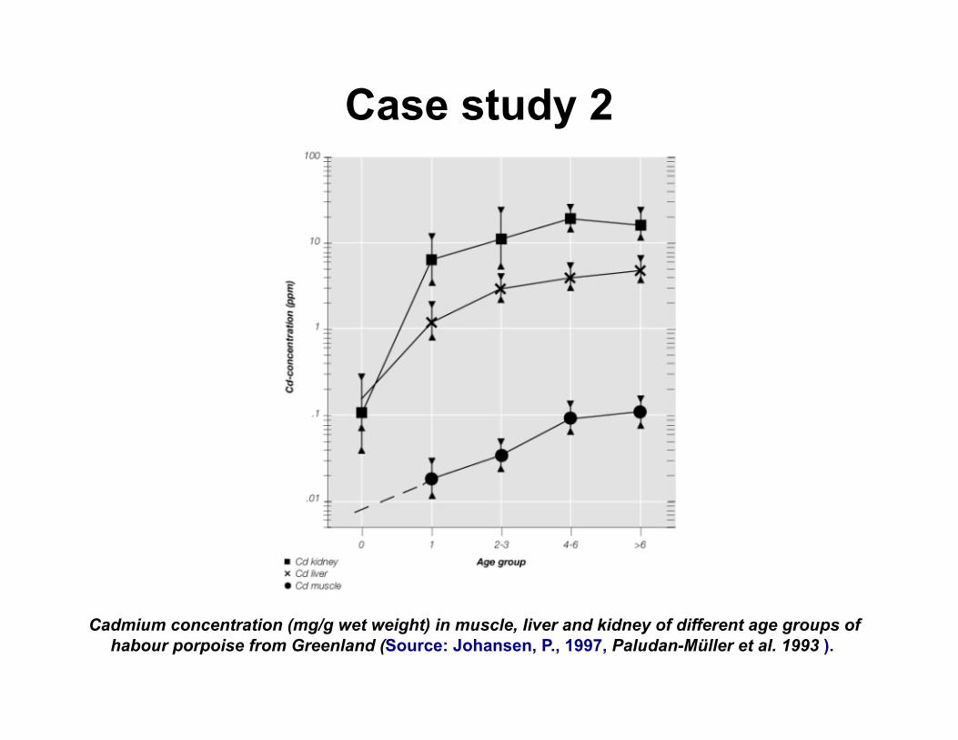
Case study 2

Cadmium concentration (mg/g wet weight) in muscle, liver and kidney of different age groups of habour porpoise from Greenland (Source: Johansen, P., 1997, Paludan-Müller et al. 1993 ).

Case study 3

Day 2: wrap-up

•  Common trends among case studies •  Overview of factors that affect biomagnification •  There is no away (persistence in the environment)

Assessments

•  Pre-test (formative) •  Post-test (summative) •  Think-pair-share (formative, not graded) •  Graded exam question(s)

Feedback

•  Please make any editorial comments on the material & return to the team

•  Did we ask the right questions on the pre-test? •  Did the handouts have enough information for

the tasks? •  Should the pre-test and post-tests be identical?

•  Timing of post-test administration

Pretest Biomagnification: You are what you eat- but don’t excrete

1. What does the arrangement of the

bottom of the graph – “trophic level” mean?

a. As you go from left to right the organisms are feeding at higher positions in the food chain

b. Higher trophic levels indicates smaller organisms

c. Trophic levels indicate the position in the ecosystem: lower level organisms live at the bottom of the lake, higher level organisms at the surface of the lake

d. The consumers are to the left and the producers to the right

2. What would be the approximate

average concentration of PCBs in a fish at trophic level 3?.

a. 0 b. 1 ng/g c. 10 ng/g d. 100 ng/g

3. What is the general trend in this

graph? a. There is no change in PCB

concentration between trophic levels.

b. Higher trophic levels have higher concentrations of PCBs

c. Lower trophic levels have higher concentrations of PCBs

4. Biomagnification is: a. As you go up a food chain the organisms tend to get larger b. The increased toxin concentrations in the tissues of organisms at higher trophic levels is

because they are bigger and eat more. c. The increased toxin concentrations in the tissues of organisms higher on the food chain is

because they are eating organisms that have higher concentrations. d. Toxins are microscopic, but their effects are “magnified” by living things.

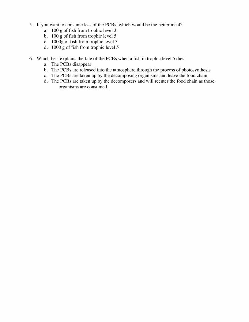
5. If you want to consume less of the PCBs, which would be the better meal? a. 100 g of fish from trophic level 3 b. 100 g of fish from trophic level 5 c. 1000g of fish from trophic level 3 d. 1000 g of fish from trophic level 5

6. Which best explains the fate of the PCBs when a fish in trophic level 5 dies:

a. The PCBs disappear b. The PCBs are released into the atmosphere through the process of photosynthesis c. The PCBs are taken up by the decomposing organisms and leave the food chain d. The PCBs are taken up by the decomposers and will reenter the food chain as those

organisms are consumed.

Posttest Biomagnification: You are what you eat- but don’t excrete.

(two versions – mix and match)

1. What does the arrangement of the bottom of the graph – “trophic level” mean?

a. As you go from left to right the organisms are feeding at higher positions in the food chain

b. Higher trophic levels indicates smaller organisms c. Trophic levels indicate the position in the ecosystem: lower level organisms live at the

bottom of the lake, higher level organisms at the surface of the lake d. The consumers are to the left and the producers to the right

2. What would be the approximate average concentration of DDT in a fish at trophic level 3?

a. 0 ppm b. 5 - 10 ppm c. 10 – 40 ppm d. 75 ppm

3. What is the general trend in this graph?

a. There is no change in DDT concentration between trophic levels. b. Higher trophic levels have higher concentrations of DDT c. Lower trophic levels have higher concentrations of DDT

4. Biomagnification is: a. As you go up a food chain the organisms tend to get larger b. The increased toxin concentrations in the tissues of organisms at higher trophic levels is

because they are bigger and eat more.

Data in figure from: Enger, E., F.C. Ross and D. B. Bailey (2005). Concepts in biology. 11th ed. Boston: McGraw Hill., p. 298

c. The increased toxin concentrations in the tissues of organisms higher on the food chain is because they are eating organisms that have higher concentrations.

d. Toxins are microscopic, but their effects are “magnified” by living things.

5. If you want to consume less DDT, which would be the better meal? a. 100 g of fish from trophic level 2 b. 100 g of fish from trophic level 4 c. 1000g of fish from trophic level 2 d. 1000 g of fish from trophic level 4

6. Which best explains the fate of the DDT when a fish in trophic level 4 dies?

a. The DDT disappears b. The DDT is released into the atmosphere through the process of photosynthesis c. The DDT is taken up by the decomposing organisms and leave the food chain d. The DDT is taken up by the decomposers and will reenter the food chain as those

organisms are consumed.

Alternative Pretest Questions

1. What are trophic levels?

2. Estimate the average DDT concentration in ppm for a fish from trophic level 3 and explain your reasoning.

3. Describe the general trend in the graph. What is happening to the concentration of DDT as the

trophic level increases?

4. Define biomagnification.

4. Explain why it would be safer to eat a fish from trophic level 2 than from trophic level 4, even if they were the same size.

6. What happens to the DDT when a fish from trophic level 4 dies?

Answers: 1. Correct answer is A. “As you go from left to right the organisms are feeding at higher positions in

the food chain”. Trophic level is a measure of position in the food chain,. Producers (photosynthesizing organisms) are at the lowest trophic levels. Secondary or tertiary consumers, that feed on other heterotrophs, are toward the top of food chains and are therefore at higher trophic levels.

2. Correct answer is C “20-40 ppm”. This data has more variance, particularly in trophic level 3, but

the average concentration should be identifiable as less than half way up the y – axis.

3. Correct answer is B. “Higher trophic levels have higher concentrations of DDT”. The general trend is an upward slope, or a positive correlation. As the trophic level increases, the concentration of DDT is higher. The large variance in trophic level 3 may be confusing, but the average concentration of 4 is clearly higher than 2.

4. The correct answer is C. “The increase in concentration of a toxin in the tissue of organisms higher

on the food chain because they are eating organisms that have higher concentrations.” Organisms higher on the food change do tend to be bigger and life longer, accumulating more toxins, but biomagnification refers to the increasing concentrations resulting from each higher trophic level feeding on more concentrated tissue.

5. The correct answer is A. “100 g of fish from trophic level 3” It is safer to feed from a lower trophic

level because, on average, the tissue is less concentrated in the toxin, and therefore you will take less into your body.

6. The correct answer is D. “The DDT is taken up by the decomposers and will reenter the food chain

as those organisms are consumed.” Some complex organic toxins might eventually be broken down, but others, and all elemental materials (lead, mercury, cadmium, etc), can not be broken down. They may be sequestered in sediments, but they may reenter the food chain through uptake by autotrophs or consumption of decomposing organisms.

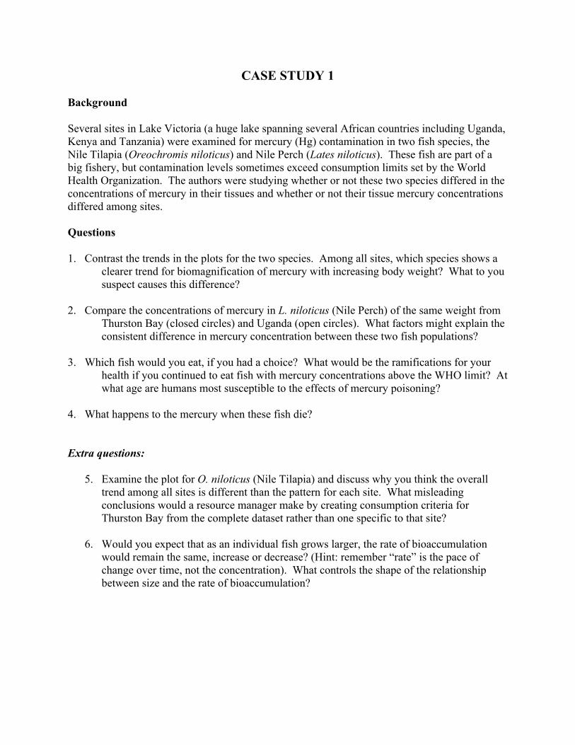
CASE STUDY 1 Background Several sites in Lake Victoria (a huge lake spanning several African countries including Uganda, Kenya and Tanzania) were examined for mercury (Hg) contamination in two fish species, the Nile Tilapia (Oreochromis niloticus) and Nile Perch (Lates niloticus). These fish are part of a big fishery, but contamination levels sometimes exceed consumption limits set by the World Health Organization. The authors were studying whether or not these two species differed in the concentrations of mercury in their tissues and whether or not their tissue mercury concentrations differed among sites. Questions 1. Contrast the trends in the plots for the two species. Among all sites, which species shows a

clearer trend for biomagnification of mercury with increasing body weight? What to you suspect causes this difference?

2. Compare the concentrations of mercury in L. niloticus (Nile Perch) of the same weight from

Thurston Bay (closed circles) and Uganda (open circles). What factors might explain the consistent difference in mercury concentration between these two fish populations?

3. Which fish would you eat, if you had a choice? What would be the ramifications for your

health if you continued to eat fish with mercury concentrations above the WHO limit? At what age are humans most susceptible to the effects of mercury poisoning?

4. What happens to the mercury when these fish die? Extra questions:

5. Examine the plot for O. niloticus (Nile Tilapia) and discuss why you think the overall trend among all sites is different than the pattern for each site. What misleading conclusions would a resource manager make by creating consumption criteria for Thurston Bay from the complete dataset rather than one specific to that site?

6. Would you expect that as an individual fish grows larger, the rate of bioaccumulation would remain the same, increase or decrease? (Hint: remember “rate” is the pace of change over time, not the concentration). What controls the shape of the relationship between size and the rate of bioaccumulation?

Campbell, L.M., J.S. Balirwa, D.G. Dixon and R.E. Hecky. 2004. Biomagnification of mercury in fish from Thruston Bay, Napoleon Gulf, Lake Victoria (East Africa. African J Aquatic Science 29(1): 91-96

CASE STUDY 2 Background Trace heavy metals, such as cadmium (Cd), occur naturally in the Earth's crust but human activities such as mining, industrial use, sewage disposal, and hydro-projects have greatly increased the mobilization and bioavailability of metals. Moreover, this has increased the chances for organisms to be exposed to harmful heavy metal concentrations. While natural baseline levels of trace heavy metals in air, soil, rivers, lakes, and oceans are usually low, trace heavy metals can become toxic to many living organisms at sufficiently high concentrations. The major source of human exposure to trace heavy metals in the environment is from food. The graph below is from a study which examined cadmium levels in Greenland marine organisms, including marine mammals. They found an overall trend of higher cadmium levels in the tissues of organisms at higher trophic levels, with the highest Cd concentrations in seabirds, seals, whales and polar bears. Within any one species, Cd concentrations are lowest in muscles, intermediate in the liver and highest in the kidneys.

Questions

1. Why do older porpoises have greater concentrations of cadmium in their tissues than younger porpoises?

2. Why does the rate of cadmium accumulation level off as a porpoise ages? Should the concentration ever decrease with age? If not, explain the apparent decrease in kidney concentrations between the ages 4-6 and age 6.

3. How would the type of tissue sampled affect a resource manager’s conclusions about heavy metal toxicity in porpoise populations? Would it matter what age class of porpoise was sampled if kidney concentrations were used? What if muscle concentrations were used instead: would this affect the conclusions drawn from the data?

4. What happens to the cadmium if a shark consumed an aging porpoise and subsequently died?

Figure 5. Cadmium concentration (µg/g wet weight) in muscle, liver and kidney of different age groups of habour porpoise from Greenland ( from Paludan-Müller et al. 1993).

Source: Johansen, P., 1997. Heavy metals in Greenland, an evaluation of data. In Thorling, L.B. and Hansen, J.C. (Eds.): Food Tables for Greenland. Inussuk-Arctic Research Journal 4: 57-71

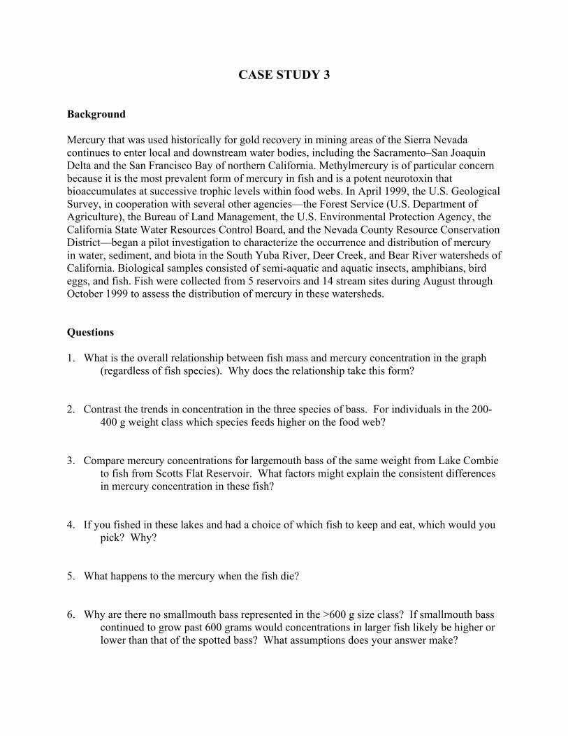
CASE STUDY 3 Background Mercury that was used historically for gold recovery in mining areas of the Sierra Nevada continues to enter local and downstream water bodies, including the Sacramento–San Joaquin Delta and the San Francisco Bay of northern California. Methylmercury is of particular concern because it is the most prevalent form of mercury in fish and is a potent neurotoxin that bioaccumulates at successive trophic levels within food webs. In April 1999, the U.S. Geological Survey, in cooperation with several other agencies—the Forest Service (U.S. Department of Agriculture), the Bureau of Land Management, the U.S. Environmental Protection Agency, the California State Water Resources Control Board, and the Nevada County Resource Conservation District—began a pilot investigation to characterize the occurrence and distribution of mercury in water, sediment, and biota in the South Yuba River, Deer Creek, and Bear River watersheds of California. Biological samples consisted of semi-aquatic and aquatic insects, amphibians, bird eggs, and fish. Fish were collected from 5 reservoirs and 14 stream sites during August through October 1999 to assess the distribution of mercury in these watersheds. Questions 1. What is the overall relationship between fish mass and mercury concentration in the graph

(regardless of fish species). Why does the relationship take this form?

2. Contrast the trends in concentration in the three species of bass. For individuals in the 200-400 g weight class which species feeds higher on the food web?

3. Compare mercury concentrations for largemouth bass of the same weight from Lake Combie to fish from Scotts Flat Reservoir. What factors might explain the consistent differences in mercury concentration in these fish?

4. If you fished in these lakes and had a choice of which fish to keep and eat, which would you

pick? Why? 5. What happens to the mercury when the fish die? 6. Why are there no smallmouth bass represented in the >600 g size class? If smallmouth bass

continued to grow past 600 grams would concentrations in larger fish likely be higher or lower than that of the spotted bass? What assumptions does your answer make?

May, J. T., R.L. Hothem, C.N. Alpers and M.A. Law. 2000. Mercury Bioaccumulation in Fish in a Region

Affected by Historic Gold Mining: The South Yuba River, Deer Creek, and Bear River Watersheds, California 1999, USGS Report 00-367.

Community factors influencing biomagnification Expert Group __ Several population or community factors may influence the concentrations of toxins in a given species or individual, independent of the general trend of higher trophic level organisms having higher concentrations of toxins. Age, size, and feeding behaviors all influence food sources, and therefore ingestion, of toxins. In general, larger organisms feed higher on the food chain, though there are many exceptions. Since most organisms get larger through their life span, older organisms will tend to be larger, feed higher on food chains, and have higher concentrations of toxins found in their food supply. Older organisms have also been living and eating longer, giving them more time to accumulate toxins. Some organisms go through significant changes through their life histories, perhaps changing their place in a food chain from, for example, a larval to an adult stage. Omnivores naturally shift among food sources from different trophic levels. Individuals within a species may vary in their primary food source in the same system, resulting in variation within the population. Finally, some members of the biotic community, decomposers, may play roles in the availability of toxins. For example, mercury exists in different forms in the ecosystem, and some forms are more easily taken up by organisms than other forms. Some forms of mercury are less abundant and may reside in sediments, thereby kept out of the food chain. Bacteria play a role in changing mercury to a form more easily absorbed by and therefore more likely to accumulate in organisms, increasing the potential that mercury will be magnified up the food chain. The bacteria convert mercury under anoxic (low oxygen) conditions. Therefore, both the members of the biotic community and abiotic environmental conditions can influence the degree of biomagnification in a given situation. Expert Discussion – Guiding question

1. For your topic, list at least five factors or conditions that might create complexity, or cause the expected relationship between trophic levels and biomagnification to vary.

Physiological factors influencing biomagnification Expert Group __ Several factors at the physiological level of the organisms may influence the concentrations of toxins in a given species or individual, independent of the general trend of higher trophic level organisms having higher concentrations of toxins. These may include where the toxin is stored in the organism, the toxic response of the organism, and possible multiple pathways for ingestion of the toxin. Most toxins have a particular point in the body where they are stored, such as in fat tissue, or in an organ like the liver. Therefore, if the entire organism is not consumed, only a portion of the toxin in the prey may move up the food chain. Also, when we sample only particular tissues without taking this differential storage into consideration, we can underestimate toxin concentrations. Toxins accumulate in organisms through both direct and indirect pathways. Primary producers may directly assimilate the toxins from the soil (i.e., rooted plants) or water (i.e., algae). Consumers may assimilate toxins directly through respiration (e.g. fish accumulate toxins through their gills as they respire) or indirectly through consumption of contaminated prey. Once heavy metal toxins are assimilated, they are not excreted and instead accumulate as the organism ages. As toxin concentrations increase in the body, organisms are increasingly susceptible to disease, neurotoxic damage, organ failure and a variety of other health problems depending on the particular toxin. Older cohorts within a population feed higher on the food web, and may therefore experience increased mortality rates as a result of prior exposure. Mercury (Hg) is a heavy metal that can damage the nervous system. In areas where humans regularly consume fish or birds highly contaminated with mercury, neurotoxicological effects of poisoning have been well documented. For pregnant women that ingest contaminated foods, the developing nervous system of the fetus may be particularly susceptible to damage from mercury. Mothers with no symptoms of mercury poisoning may give birth to infants with severe disabilities, or may expose infants to mercury through breast feeding. These effects extend beyond childbirth; children exposed to mercury while in utero have been shown to score lower on standardized tests and to experience delayed development. Cadmium (Cd) accumulates in the human kidneys, and low level exposure over long periods can result in kidney damage. Cadmium has also been shown to produce osteomalacia in children, a painful bone disorder similar to rickets. Cadmium is also a carcinogen. Expert Discussion – Guiding question

1. For your topic, list at least five factors or conditions that might create complexity, or cause the expected relationship between trophic levels and biomagnification to vary.

Ecosystem and landscape factors influencing biomagnification Expert Group __ Several landscape or ecosystem-level factors may influence toxin concentrations in an individual or species, independent of the general trend of higher trophic level organisms having higher concentrations of toxins. The location of toxin sources influences their distribution across the landscape; sources can be either “point source” (having identifiable points of origin, such as in a storm drain or factory drain pipe) or “nonpoint source” (diffuse points of origin, such as runoff from land or atmospheric deposition). The highest toxin concentration will be found closest to a source, with higher concentrations near point sources compared to nonpoint sources. Plants and animals living close to toxin sources are likely to have higher toxin concentrations compared to organisms living further from these sources. Plants and animals can also change the way a toxin is spread across the landscape. For example, wetland plants and sediments surrounding a body of water can absorb toxins entering in runoff before they reach the water body itself, in a process known as “buffering”. A buffered lake, therefore, should have lower toxin concentrations in its waters compared to a lake without these buffers. The organisms living in a buffered lake should have lower toxin concentrations in their tissues than organisms from an unbuffered lake. Even a lake with a point source of a toxin could have low toxin concentrations in its waters if it is surrounded by buffering plants and sediments. Therefore, one must take multiple factors into account when considering the likelihood of high toxin concentrations and biomagnification in a landscape or ecosystem. Two toxins that are unevenly spread across the landscape are cadmium (Cd) and mercury (Hg). Cadmium enters the environment from both natural and anthropogenic (human-caused) sources. The natural sources of Cd include the weathering and mining of rocks and minerals that contain cadmium. Anthropogenic sources of Cd include the mining and electroplating industries, which either use or produce Cd, as well as cigarette smoke. Cadmium enters water bodies or the atmosphere as a result of these sources, and organisms are exposed directly in the water, through inhalation, exposure from atmospheric deposition on soils or other surfaces, or through the consumption of plants or animals that have accumulated Cd in or on their tissues. Mercury (Hg) is emitted into the atmosphere through anthropogenic sources, such as manufacturing or burning coal for fuel, and from natural sources, such as volcanoes. Atmospheric Hg can be transported over a range of distances, potentially resulting in deposition on local, regional, continental and/or global scales. The availability of Hg for uptake by organisms is dependent upon the conversion of inorganic Hg into methylmercury by bacteria. Once Hg is converted into methylmercury, it can accumulate up the food chain in fish, fish-eating animals, and people. Expert Discussion – Guiding question

1. For your topic, list at least five factors or conditions that might create complexity, or cause the expected relationship between trophic levels and biomagnification to vary.

Think-Pair-Share Activity Intraspecific variation in response to toxins

Mercuryconcentrationsvs.lengthinwalleyefromSouthManistiqueLakeFrom:Fishcontaminantmonitoringprogram:reviewandrecommendations.2003.Report

preparedbyExponent(Bellevue,WA)fortheMichiganDepartmentofEnvironmentalQuality,Lansing,Michigan,Doc.no.8601969.00105010103BH29.

Thinkaboutyouranswerstothesequestions,thenturntoyourneighborandshareyouranswers 1. Describe the overall trend, if any, of mercury concentration with fish length.

2. If you saw a trend in the data, what could explain the trend?

3. How much mercury is there in a walleye fish that is 18 inches long?

4. Why might different fish of the same size have different mercury concentrations?

Minute paper topics

1. Compare the graph above to the one in the Pretest. How do these data fit into the pattern you saw in the Pretest graph?

2. If you worked for the Environmental Protection Agency and you had to tell people how much walleye they could safely eat, how would you decide what size of fish is safe?

3. Would you get a very different dose of mercury if you ate the same mass of fish from a lower trophic level than walleye? Explain your reasoning?

Examples of topics students should cover in their minute papers

1. They should identify the difference between this graph, which shows data for only one species, and the Pretest graph which shows many trophic levels. They should discuss variability within a species, and should be able to say that despite intraspecific variation, the pattern of biomagnification across trophic levels is strong enough to be evident despite this variability.

2. This question should elicit answers that discuss skepticism in specific “safe” levels of mercury as measured by a size or weight of fish one can eat. The conservative answer would state that if limits are to be set, one should err on the side of caution and suggest that people eat less, or smaller, fish. An observant student would notice that the scatter in the data are sufficient to warrant skepticism about setting limits based on fish size. Looking at the walleye graph, fish between about 16 and 22 inches can have any of a number of mercury concentrations. It’s not clear that a 16” fish is any more likely to have less mercury than a 22” fish.

3. For this question, students would need to think back to the Pretest graph and put this graph into that context. They would have to recall trophic levels and how biomagnification works from that exercise. What should be different in their answer, now that they’ve seen the walleye graph, is a discussion of intraspecific variation and how that can “blur” the otherwise clear pattern of biomagnification with trophic level. Asking this question at this point allows the instructor to make sure students don’t see this intraspecific variability and think it translates into NO pattern with trophic level. This gives the instructor the chance to point out how biomagnification is a strong enough process that it’s clearly visible despite variability at the level of the species or population.

Biomagnification unit Instructor’s Manual – answers to questions

Pretest

1. Correct answer is A. “As you go from left to right the organisms are feeding at higher positions in the food chain”. Trophic level is a measure of position in the food chain. Producers (photosynthesizing organisms) are at the lowest trophic levels. Secondary and tertiary consumers, which both feed on other heterotrophs, are toward the top of food chains and are therefore at higher trophic levels.

2. Correct answer is C “10 ng/g”. From the trophic level three position on the x-axis,

extend a line straight up to the response curve line, the blue line on the graph. The lines will intersect at approximately 10.

3. Correct answer is B. “Higher trophic levels have higher concentrations of PCBs”. The

general trend is an upward slope, or a positive correlation. As the trophic level increases, the concentration of PCBs is higher. Although there is some variation in the individual data points, the trend is clear.

4. The correct answer is C. “The increase in concentration of a toxin in the tissue of

organisms higher on the food chain because they are eating organisms that have higher concentrations.” Organisms higher on the food chain do tend to be bigger and live longer, thereby accumulating more toxins, although this is not what is known as biomagnification. Biomagnification refers to the increase in toxin concentrations with increases in trophic level, which results from each higher trophic level feeding on tissues with greater toxin concentrations.

5. The correct answer is A. “100 g of fish from trophic level 3” It is safer to feed from a

lower trophic level because, on average, the tissue is less concentrated in the toxin, and therefore you will take less into your body. In addition, a smaller mass of fish will yield a lower total amount of toxin ingested.

6. The correct answer is D. “The PCBs are taken up by the decomposers and will reenter the

food chain as those organisms are consumed.” Some complex organic toxins might eventually be broken down, but others, and all elemental materials (lead, mercury, cadmium, etc), can not be broken down. They may be sequestered in sediments, but they may reenter the food chain through uptake by autotrophs or consumption of decomposing organisms. It is important to stress in subsequent discussions that toxins may move through food chains but are not “lost” to the system.

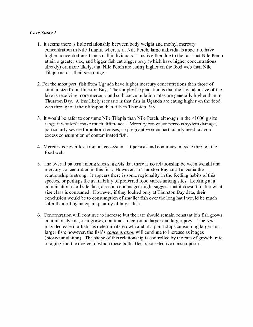
Case Study 1

1. It seems there is little relationship between body weight and methyl mercury concentration in Nile Tilapia, whereas in Nile Perch, large individuals appear to have higher concentrations than small individuals. This is either due to the fact that Nile Perch attain a greater size, and bigger fish eat bigger prey (which have higher concentrations already) or, more likely, that Nile Perch are eating higher on the food web than Nile Tilapia across their size range.

2. For the most part, fish from Uganda have higher mercury concentrations than those of

similar size from Thurston Bay. The simplest explanation is that the Ugandan size of the lake is receiving more mercury and so bioaccumulation rates are generally higher than in Thurston Bay. A less likely scenario is that fish in Uganda are eating higher on the food web throughout their lifespan than fish in Thurston Bay.

3. It would be safer to consume Nile Tilapia than Nile Perch, although in the <1000 g size

range it wouldn’t make much difference. Mercury can cause nervous system damage, particularly severe for unborn fetuses, so pregnant women particularly need to avoid excess consumption of contaminated fish.

4. Mercury is never lost from an ecosystem. It persists and continues to cycle through the

food web. 5. The overall pattern among sites suggests that there is no relationship between weight and

mercury concentration in this fish. However, in Thurston Bay and Tanzania the relationship is strong. It appears there is some regionality in the feeding habits of this species, or perhaps the availability of preferred food varies among sites. Looking at a combination of all site data, a resource manager might suggest that it doesn’t matter what size class is consumed. However, if they looked only at Thurston Bay data, their conclusion would be to consumption of smaller fish over the long haul would be much safer than eating an equal quantity of larger fish.

6. Concentration will continue to increase but the rate should remain constant if a fish grows

continuously and, as it grows, continues to consume larger and larger prey. The rate may decrease if a fish has determinate growth and at a point stops consuming larger and larger fish; however, the fish’s concentration will continue to increase as it ages (bioaccumulation). The shape of this relationship is controlled by the rate of growth, rate of aging and the degree to which these both affect size-selective consumption.

Case Study 2

1. As the porpoise ages, all the cadmium it consumes remains in its body and is not excreted. In this way, cadmium bioaccumulates over time. In addition, as the porpoise ages, presumably it is also growing, and, if larger porpoise eat relatively larger prey items (that themselves have higher cadmium concentrations than smaller individuals) then the rate of increase in cadmium concentration will also increase (biomagnification).

2. Metals should continue to accumulate at a constant or exponential rate as an organism ages through bioaccumulation and biomagnification. A leveling off suggests either that the organism has stopped increasing the size of prey consumed (because its own growth rate has dropped) or it is translocating the metals to another part of the body. The apparent decrease in kidney concentrations between ages 4-6 is suggestive of the latter (i.e., muscle concentrations continue to increase) although the error bars are large enough that there may actually be no difference between these two age classes.

3. Yes, it matters what type of tissue is used in analysis. The size distribution of the sampled population also matters. If the only measurements were of muscle concentrations in younger animals, a manager might conclude that there was no problem. If kidney and liver levels were used in progressively older animals, the manager might conclude that the animal is not increasing its health risk over time. In the latter case, the manager would be overlooking the translocation or life-history change in allocation of increasingly larger amounts of metals to muscle tissue as the animal ages.

4. The cadmium is released back into the environment upon decay to be taken up again by other organisms or is directly consumed by scavenging animals or microbes. It is not lost from the environment.

Case Study 3

1. The graph shows that as fish increase in size, mercury concentration also increases. This is likely due to the fact that mercury consumed by prey and taken in through the gills is not lost as fish age (bioaccumulation) and, also, that as the fish ages, it continues to eat larger and larger prey which themselves have higher and higher concentrations in their own tissues (biomagnification). The trend should not decrease (this would suggest losses through egestion or excretion which is not physiologically probable) and the rate should continue to increase as the fish grows.

2. Mercury concentrations increase with size in all species. However, for each size class

there is a predictable and different range of concentrations among the three species. In the 200-400 g size class, largemouth bass have the lowest concentrations, smallmouth bass the next highest and spotted bass the highest mercury concentrations. This would suggest that uptake is faster in the spotted and smallmouth bass than the largemouth bass, perhaps because the former are eating larger prey (such as other small fish) than the largemouth bass (perhaps relying on invertebrate prey at this point in the life cycle).

3. Fish from Lake Combie have much higher concentrations than those of the same weight

in Scotts Flat Reservoir. Either fish from Scotts Flat are exposed to lower overall mercury concentrations than those in Lake Combie or they are eating lower on the food web, perhaps because that habitat supports more invertebrate (or smaller) consumer prey items.

4. It would be better to eat smaller fish, in general, than larger ones and better to avoid

spotted bass altogether as they can have concentrations above the FDA action level even in the smallest size classes.

5. The mercury is released back into the environment as the fish decays and re-enters the

food web through indirect or direct consumption. It is never lost from the system and continues to accumulate regardless of the current loading rate.

6. This mass (600 g) may be the largest attainable size for most smallmouth bass, or the

concentrations of mercury in their tissue is lethal at that level and so no fish above this size survive. If smallmouth bass continued to grow over 600 grams in weight, they would likely have even greater mercury concentrations in their tissues than the spotted bass. This assumes that the linear rate of increase continues throughout the life of the fish. This assumption would be true if the fish continued to eat larger and larger prey as they grow.

Posttest

1. Correct answer is a. “As you go from left to right the organisms are feeding at higher positions in the food chain”. Trophic level is a measure of position in the food chain. Producers (photosynthesizing organisms) are at the lowest trophic levels. Secondary and tertiary consumers, which both feed on other heterotrophs, are toward the top of food chains and are therefore at higher trophic levels.

2. Correct answer is c: “10-40 ppm”. These data have a good deal of variation in DDT

concentrations, particularly in trophic level 3, but the average concentration should be identifiable as less than half way up the y – axis.

3. Correct answer is b. “Higher trophic levels have higher concentrations of DDT”. The

general trend is an upward slope, or a positive correlation. As the trophic level increases, the concentration of DDT is higher. The large variance in trophic level 3 may be confusing, but the average concentration of 4 is clearly higher than 2.

4. The correct answer is c. “The increase in concentration of a toxin in the tissue of

organisms higher on the food chain because they are eating organisms that have higher concentrations.” Organisms higher on the food chain do tend to be bigger and live longer, thereby accumulating more toxins, although this is not what is known as biomagnification. Biomagnification refers to the increase in toxin concentrations with

increases in trophic level, which results from each higher trophic level feeding on tissues with greater toxin concentrations.

5. The correct answer is a. “100 g of fish from trophic level 3” It is safer to feed from a

lower trophic level because, on average, the tissue is less concentrated in the toxin, and therefore you will take less into your body. In addition, a smaller mass of fish will yield a lower total amount of toxin ingested.

6. The correct answer is d. “The DDT is taken up by the decomposers and will reenter the

food chain as those organisms are consumed.” Some complex organic toxins might eventually be broken down, but others, and all elemental materials (lead, mercury, cadmium, etc.), cannot be broken down. They may be sequestered in sediments, but they may also reenter the food chain through uptake by autotrophs or consumption of decomposing organisms.