Excusing Selfishness in Charitable Giving:

The Role of Risk

Christine L. Exley ∗

September 7, 2015

Abstract

Decisions involving charitable giving often occur under the shadow of risk. A common

finding is that potential donors give less when there is greater risk that their donation will

have less impact. While this behavior could be fully rationalized by standard economic

models, this paper shows that an additional mechanism is relevant: the use of risk as an

excuse not to give. In a laboratory study, participants evaluate risky payoffs for themselves

and risky payoffs for a charity. When their decisions do not involve tradeoffs between money

for themselves and the charity, they respond very similarly to self risk and charity risk. By

contrast, when their decisions force tradeoffs between money for themselves and the charity,

participants act more averse to charity risk and less averse to self risk. These altered

responses to risk bias participants towards choosing payoffs for themselves more often,

consistent with excuse-driven responses to risk. Additional results support the existence of

excuse-driven types.

Keywords: charitable giving; prosocial behavior; altruism; risk preferences

∗Exley, Harvard Business School; clexley@hbs.edu. Acknowledgements: I gratefully acknowledge fundingfor this study from the NSF (SES # 1159032), the Stanford Economics Department, the Stanford Center onPhilanthropy and Civil Society, and the Stanford Institute for Economic Policy Research via the E.S. Shaw& B.F. Haley Fellowship. For helpful advice, I would like to thank participants at the Stanford Institute forTheoretical Economics Workshops, the Experimental Sciences Association Annual Conferences, the StanfordBehavioral Seminars and Lunches, as well as the editor, three anonymous referees, B. Douglas Bernheim, KatherineCoffman, Lucas Coffman, Paul J. Healy, Muriel Niederle, Alvin Roth, Charles Sprenger, and Stephen Terry.

1

1 Introduction

In the United States, 1 in 4 adults volunteer and 1 in 2 adults give to charities for an estimated

combined value of $500 billion dollars per year.1 An established literature documents potential

motives for such giving; for instance, people feel good about themselves when they help others

(Andreoni, 1989, 1990), value appearing nice to others (Harbaugh, 1998a; Benabou and Tirole,

2006; Ariely et al., 2009), and desire to conform with social norms (Andreoni and Bernheim,

2009).2 These motives, as well as standard economic models, may easily explain a common

finding in charitable giving: individuals give less when when there is a greater risk that their

donation will have less impact (Brock et al., 2013; Krawczyk and Lec, 2010).3 In this paper,

however, I investigate whether an additional mechanism is relevant: do people use the risk that

their donation may have less than the desired impact as an excuse not to give?

Given how often people are asked to give – over 50% of adults report being asked more

than three times within the past year – reluctant individuals may desire an excuse not to give.4

Previous literature in fact demonstrates a large scope for motivations broadly related to excuses.

For instance, people often behave more selfishly when they can avoid learning how their decisions

affect others (Dana et al., 2007; Bartling et al., 2014; Grossman, 2014), develop self-serving biases

(Konow, 2000; Haisley and Weber, 2010), or rely on the possibility that their decisions did not

influence the outcome (Dana et al., 2007; Andreoni and Bernheim, 2009; Linardi and McConnell,

2011; Falk and Szech, 2013).5 People also achieve more selfish outcomes by delegating decisions

to others (Hamman et al., 2010; Coffman, 2011; Bartling and Fischbacher, 2012), or by avoiding

situations that involve giving decisions (Dana et al., 2006; Broberg et al., 2007; Andreoni et al.,

2011; Lazear et al., 2012; DellaVigna et al., 2012).6

This paper differentiates itself from existing literature by documenting self-serving responses

1http://www.volunteeringinamerica.gov/infographic.cfm, http://www.givingusareports.org/.2For an overview of these reasons as well as others, see surveys in Vesterlund (2006) and Andreoni (2006).3While Brock et al. (2013) and Krawczyk and Lec (2010) involve objective risk in a dictator game, other

studies document reduced giving in response to other types of risk or uncertainty, involving performance metrics(Yoruk, 2013; Meer, 2014; Brown et al., 2014; Karlan and Wood, 2014), the use of donations (Gneezy et al., 2014;Batista et al., 2015), and the recipient of donations (Small and Loewenstein, 2003; Fong and Oberholzer-Gee,2011; Li et al., 2013).

4Results are from a Google Consumer Survey I ran in Sept. - Nov. 2014. 505 individuals answered “Withinthe past year, approximately how many times have you been asked - whether in person or via other means, suchas emails or social media - to donate money to a charity?” 51% of respondents answered 3 or more times.

5van der Weele et al. (2014) documents a limitation of these results in the context of reciprocal behavior.Some of this work also ties into image motivation that often leads people to behave more selfishly when there isless observability of their action, such as discussed in Harbaugh (1998b,a); Andreoni and Petrie (2004); Benabouand Tirole (2006); Andreoni and Bernheim (2009); Ariely et al. (2009); Lacetera and Macis (2010); Linardi andMcConnell (2011); Exley (2014). There is also a relatedly rich literature in psychology on moral licensing (seeMerritt et al. (2010) for a nice overview).

6Moreover, Andreoni and Rao (2011) and Castillo et al. (2014) show that asking people to give increasesdonations. Oberholzer-Gee and Eichenberger (2008) finds that just the option to avoid giving decisions – bychoosing to play a lottery instead of a dictator game – can also lead to reduced giving.

2

to objective risk in a social setting absent other factors, such as image concerns (Andreoni and

Bernheim, 2009), information acquisition (Dana et al., 2006), ambiguity (Haisley and Weber,

2010), or actions of others (Falk and Szech, 2013). In exploiting a within-subject experimental

design, this paper also provides evidence for an individual level of consistency in self-serving

tendencies. Motivated by related policy questions, this paper somewhat less commonly focuses

on charitable giving decisions, but as verified in an additional study involving payoffs for other

participants instead of a charity, it seeks to contribute to the broader other-regarding literature.

To begin, this paper conducts a laboratory study that allows for the needed control to isolate

excuse-driven responses to risk from other responses to risk. Participants make a series of binary

decisions between risky and riskless payoffs that may benefit themselves or the American Red

Cross. A risky payoff is a lottery that yields a non-zero amount with probability P and $0 with

probability 1 − P . A risky payoff is a “charity lottery” or a “self lottery” if the corresponding

outcome is given to the American Red Cross or the participant, respectively.7 A riskless payoff

yields a non-zero amount with certainty. A riskless payoff is a “charity-certain amount” or “self-

certain amount” if it is given to the American Red Cross or to the participant, respectively. In

other words, participants face four types of binary decisions that vary according to the involved

payoffs - {self lottery, charity lottery} X {self-certain amount, charity-certain amount}.Notice that participants do not face tradeoffs between payoffs for themselves and the charity

when deciding between: (i) self lotteries and self-certain amounts, or (ii) charity lotteries and

charity-certain amounts. In this no self-charity tradeoff context, excuses not to give are irrelevant

as participants never decide whether or not to give - i.e., they cannot give in (i) or are forced to

give in (ii). By contrast, participants always face tradeoffs between payoffs for themselves and

the charity when deciding between: (iii) self lotteries and charity-certain amounts, or (iv) charity

lotteries and self-certain amounts. In this self-charity tradeoff context, excuses not to give may

be relevant. Changes in responses to risk across these contexts can thus exhibit the extent to

which excuse-driven risk preferences influence charitable giving decisions.

Figure 1 shows the main results of my study by plotting how lottery valuations change as the

probability P of the non-zero payment increases, i.e., as risk decreases. For ease of comparison,

note that the lottery valuations are scaled as percentages of the corresponding riskless lottery

valuations. In the no self-charity tradeoff context, participants’ responses to risk in self lotteries

and charity lotteries are nearly indistinguishable. From P = 1 to P = 0.5, or in response

to 50% risk of a zero-dollar outcome, participants reduce their valuations by about 50% for

both self lotteries and charity lotteries. These equivalent responses likely result in part from a

normalization, detailed later in the design, that ensures participants are indifferent between the

nonzero payoffs in the self lotteries and charity lotteries. Absent this normalization, different

7In this study, a charity lottery does not involve (any chance of) payoffs to the participants. This is differentthan incentivizing charitable giving by entering donors into a lottery that may financially benefit themselves, suchas in Landry et al. (2006).

3

responses to risk in self lotteries and charity lotteries may have resulted from participants valuing

money for themselves and the charity differently. While an emerging literature considers how

individuals’ responses to risk may differ over their own money and others’ money, this is the first

study, to my knowledge, to show equivalent responses to risk in self lotteries and charity lotteries

when corresponding payoffs are normalized.8

In the self-charity tradeoff context, by contrast, participants’ responses to self risk and charity

risk diverge. Consistent with excuse-driven risk preferences, participants act both more averse

to charity risk and less averse to self risk. In response to 50% risk, participants reduce their

valuations by only 40% for self lotteries but by 60% for charity lotteries. The most stark findings,

however, occur with the introduction of even small risk. From P = 1 to P = 0.95, or in response

to only 5% risk of a zero-dollar outcome, participants’ valuations for charity lotteries decrease by

32% in the self-charity tradeoff context. The reduction is four times larger than the corresponding

8% decrease in the no self-charity tradeoff context. That is, participants appear to overweight

the possibility that charity lotteries yield zero-dollar payoffs, using it as an excuse to choose self

certain-amounts over charity lotteries.

Figure 1: Preview of Results

No Self-Charity Tradeoff

010

2030

4050

6070

8090

100

Valu

atio

n as

% o

f Ris

kles

s Lo

ttery

0 .1 .2 .3 .4 .5 .6 .7 .8 .9 1Probability P of Non-Zero Payment

Self Lottery

Charity Lottery

Expected Value

Self-Charity Tradeoff

010

2030

4050

6070

8090

100

Valu

atio

n as

% o

f Ris

kles

s Lo

ttery

0 .1 .2 .3 .4 .5 .6 .7 .8 .9 1Probability P of Non-Zero Payment

Self Lottery

Charity Lottery

Expected Value

I infer from the observed treatment effects that individuals exhibit excuse-driven risk prefer-

ences. By exploiting the within-subject design of this study, additional results provide evidence

for excuse-driven types of participants and hence contribute to limiting the scope for non-excuse-

driven explanations. First, participants who appear more selfish in riskless decisions are more

8For instance, related literature includes (Andersson et al., 2013, 2014; Bolton and Ockenfels, 2010; Brennanet al., 2008; Chakravarty et al., 2011; Eriksen et al., 2014; Guth et al., 2008). More specific to the charitablegiving domain, although not risk, Exley and Terry (2015) and Bernheim and Exley (2015) show that behavioralmotivations, involving reference-dependent behavior or norms, differ when earning money for oneself as opposedto for a charity.

4

likely to also exhibit excuse-driven risk preferences in risky decisions. Second, participants with

excuse-driven risk preferences are more likely to engage in other excuse behavior in a separate

incentivized “moral wiggle room” task, as developed in Dana et al. (2007). While excuse-driven

risk preferences involve unambiguously selfish decisions – by choosing self payoffs over charity

payoffs more often – excuse-driven behavior in the moral wiggle room task involves avoiding

information on whether or not decisions are selfish.

In an additional study, I test whether my results are more broadly relevant to prosocial

behavior, as opposed to just charitable giving. I find strong evidence for excuse-driven risk

preferences when participants decide between payoffs for themselves and payoffs for another

study participant, as opposed to payoffs for a charity.

This paper proceeds as follows. Section 2 overviews the predictions according to the channels

through which risk influences giving, Section 3 details the experimental design, Section 4 describes

the results, and Section 5 concludes by highlighting further avenues for research.

2 Predictions

To determine through which channels risk influences charitable giving decisions, I elicit partici-

pants’ valuations of various self lotteries and charity lotteries. Participants receive the outcomes

of self lotteries; the American Red Cross (ARC) receives the outcomes of charity lotteries. A

“self lottery,” denoted by P s, yields $10 for a participant with probability P and $0 for a partic-

ipant with probability 1− P . A “charity lottery,” denoted by P c, yields $X for the charity with

probability P and $0 for the charity with probability 1− P . To ensure that charity lotteries are

comparable to self lotteries, I determine participant-specific X values such that participants are

indifferent between themselves receiving $10 with certainty and the charity receiving $X with

certainty. In other words, if (U, V ) represents a bundle where a participant receives $U and the

charity receives $V, then this study will yield valuations for:

P (10, 0) + (1− P )(0, 0)︸ ︷︷ ︸P s: self lottery with probability P

and P (0, X) + (1− P )(0, 0)︸ ︷︷ ︸P c: charity lottery for probability P

where

(10, 0) ∼ (0, X), and P ∈ {0.05, 0.1, 0.25, 0.5, 0.75, 0.9, 0.95}.

Valuations of self lotteries are denoted as Y j(P s), and valuations of charity lotteries are de-

noted as Y j(P c). The superscript j indicates whether lottery valuations are self-dollar valuations

(j = s) or charity-dollar valuations (j = c). Self-dollar valuations are in dollars given to par-

ticipants, and charity-dollar valuations are in dollars given to the charity. The resulting four

types of lottery valuations, summarized in Table 1 and explained below, allow me to distinguish

5

Table 1: Types of Lottery Valuations Resulting from Binary Decisions

Self-CertainAmount

Charity-CertainAmount

Self Lottery Y s(P s) Y c(P s)

Charity Lottery Y s(P c) Y c(P c)

No Self-Charity Tradeoff ContextSelf-Charity Tradeoff Context

between three channels through which risk may influence giving.

In the no self-charity tradeoff context, valuations result from decisions involving no tradeoffs

between payoffs for the participants and the charity. Y s(P s) is the valuation such that par-

ticipants are indifferent between themselves receiving $Y s(P s) with certainty and themselves

receiving the outcome of P s. Y c(P c) is the valuation such that participants are indifferent be-

tween the charity receiving $Y c(P c) with certainty and the charity receiving the outcome of P c.

In the self-charity tradeoff context, valuations result from decisions involving tradeoffs between

payoffs for the participants and the charity. Y c(P s) is the valuation such that participants are

indifferent between the charity receiving $Y c(P s) with certainty and themselves receiving the

outcome of P s. Y s(P c) is the valuation such that participants are indifferent between themselves

receiving $Y s(P c) with certainty and the charity receiving the outcome of P c.

Since self-dollar valuations and charity-dollar valuations are elicited in different units, I con-

sider valuations scaled as a percentage of the riskless lottery valuation. Self-dollar valuations

(Y s(P s) or Y s(P c)) are scaled as percentages of $10 being given to the participants. Charity-

dollar valuations (Y c(P c) or Y c(P s)) are scaled as percentages of $X being given to the charity.

In the following predictions and discussion of my results, I assume linear utility in payoffs as

doing so allows for such rescaling. However, my results are robust to interpretations that do not

rely on this rescaling.9

Since participant-specific X values imply (10, 0) ∼ (0, X), several models imply that partic-

ipants should be indifferent between charity lotteries and self lotteries as they merely introduce

the same 1− P probability of a $0 outcome. That is:

P (10, 0) + (1− P )(0, 0)︸ ︷︷ ︸P s: self lottery with probability P

∼ P (0, X) + (1− P )(0, 0)︸ ︷︷ ︸P c: charity lottery for probability P

, ∀P. (1)

For instance, this indifference is directly implied by the independence axiom, as in von

Neumann-Morgenstern expected utility, and corresponds with what I define as standard risk

preferences.

9See footnote 19 for more complete discussion in light of my empirical findings.

6

Prediction 1 (Standard Risk Preferences) All else equal, if participants have standard

risk preferences for some probability P , then

Y s(P s) = Y c(P s) = Y c(P c) = Y s(P c).

By contrast, if participants have what I define as charity-specific risk preferences, the indif-

ference shown in relation 1 may not hold. For instance, in his theory of good intentions, Niehaus

(2014) proposes that individuals may receive a “warm glow” or good feeling from thinking they

did good. In some cases, such warm glow giving could cause participants to hold optimistic

beliefs about the impact of their donations and respond less to different charity risk levels. More

generally, charity-specific risk preferences may result if participants’ risk preferences or behavioral

responses to risk differ for self payoffs and charity payoffs.

Prediction 2 (Charity-Specific Risk Preferences) All else equal, if participants have charity-

specific risk preferences for some probability P , then

Y s(P s) = Y c(P s) 6= Y c(P c) = Y s(P c).

By contrast, excuse-driven risk preferences allow for the possibility that the same charity lot-

tery or the same self lottery may be valued differently depending on whether the context permits

excuses not to give. In the no self-charity tradeoff context, participants never trade off payoffs for

themselves with payoffs for the charity, so excuse-driven risk preferences are not relevant. How-

ever, in the self-charity tradeoff context, participants must trade off payoffs for themselves with

payoffs for the charity, so excuse-driven risk preferences would bias them towards choosing pay-

offs for themselves. When participants decide between charity lotteries and self-certain amounts,

they may overweight the possibility that charity lotteries yield zero-dollar charity payoffs as an

excuse to choose the self-certain amounts over charity lotteries. A resulting increased aversion

to charity risk would yield lower charity lottery valuations relative to those in the no self-charity

tradeoff context. Alternatively, when participants decide between self lotteries and charity-certain

amounts, they may favor the possibility that self lotteries yield non-zero self payoffs as an excuse

to choose self lotteries over charity-certain amounts. A resulting decreased aversion to self risk

would yield higher self lottery valuations relative to those in the no self-charity tradeoff context.

Prediction 3 (Excuse-Driven Risk Preferences) All else equal, if participants have excuse-

driven risk preferences for some probability P , then

Y s(P s) = Y c(P c),

but

Y c(P s) > Y s(P s) and Y c(P c) > Y s(P c).

7

3 Data and Design

There are two versions of my study. While Section 3.1 highlights my main study that involves

charitable giving decisions, Section 3.2 details a modified version of the study that involves giving

to another participant in the study, as opposed to a charity.

3.1 Charitable Giving Study

From November 2013 - January 2014, I recruited one-hundred undergraduate students to partic-

ipate in one of five study sessions via the Stanford Economics Research Laboratory. Each study

session adhered to the following design.

After participants listen to instructions and correctly answer several understanding questions,

they complete thirty price lists.10 Each price list involves a series of binary decisions, from

which one randomly selected decision is implemented for payments and added to their minimum

participation fee of $20.11 After participants complete these price lists, they answer several follow-

up questions, which include demographic questions and moral wiggle room questions described

later (see Section 4.3). Participants are then paid in cash and exit the study. All decisions in

this study remain anonymous. Participants complete this study on laptops, via an online survey

platform called Qualtrics, in the Stanford Economics Research Laboratory.

Participants first complete a “normalization” price list that determines participant-specific

X values such that they are indifferent between $10 for themselves and $X for the charity.

Participants are unaware that their choices in the normalization price list determine the non-zero

payoff they will later face in decisions involving charity lotteries. Instead, in the normalization

price list, they are just asked to make sixteen binary decisions between two Options (A and B).12

Option A always involves the participants receiving $10 with certainty. However, as they proceed

down the sixteen rows of the price list, Option B increases from the charity receiving $0, $2, ...,

to $30 with certainty. See Appendix A.1 for a screenshot of the normalization price list.

From participants’ decisions in the normalization price list, I estimate participant-specific X

values as follows. Assume a participant switches from choosing Option A to Option B on the ith

row, and that this corresponds to the charity receiving $Bi. It then follows that Bi−1 ≤ X ≤ Bi,

10If they incorrectly answer a question, they are redirected to answer it again until they provide the correctanswer. At this time, they may also ask any questions to the study leader.

11Implementing payoffs from one row of multiple price lists (MPLs) is a common experimental procedure thatis incentive compatible if one assumes sufficiently narrow framing, or as discussed in Azrielli et al. (2014), if oneassumes dominated lotteries are never chosen. Also, if one considers this payment mechanism a compound lottery,then my observed treatment effects are difficult to rationalize since any given decision has less than a 0.2 percentchance of being implemented.

12Nonetheless, imagine that participants could forecast this feature of the study. Unless a participant derivesdisutility from the charity receiving higher donations, there is no motivation to make choices such that X wouldbe underestimated. On the other hand, if participants overestimate X, then this would bias my results againstbeing able to find evidence for excuse-driven risk preferences, as discussed in footnote 13.

8

and I estimate X as its upper bound of Bi. I choose the upper bound as overestimations of X

bias my results against finding evidence for excuse-driven risk preferences.13

There are two cases where X cannot be accurately estimated in my data. The first case

involves “multiple switch points.” Although Option A is fixed and Option B increases as a par-

ticipant proceeds down the rows of the price list, a participant may choose Option B on row i

but may not choose a higher valued Option B on some later row i + j, implying a violation of

monotonicity in preferences. Only one participant has multiple switch points in the normaliza-

tion price list, and this participant will be excluded from the remaining analysis. The second

case involves “censored X values,” which occur if a participant never chooses Option B, or al-

ways chooses $10 for themselves over the charity receiving any amount up to $30. Forty-two

participants (out of the one-hundred participants) have censored X values. This occurrence is

comparable to Engel (2011)’s meta study finding that 36% of dictators never give any positive

amount – which normally could be as little as $1 – to their recipients in dictator games. My main

results exclude participants with censored X values, although my results are robust to including

this group by assuming their X values are equal to their lower bound of $30.

Therefore, my main results are likely most relevant among a population interested in donating

to the charity in this study, i.e., the American Red Cross. This explanation is bolstered by

participants’ decisions in a second price list that serves as a buffer between the normalization

task and valuation tasks. Participants complete the second price list immediately after the

normalization price list, and it only differs by replacing the $10 payoff for participants in Option

A with a $5 payoff for participants. In return, I find that 69% of participants with censored X

values are also unwilling to give up $5 for themselves in order for the charity to receive $30. Even

among participants without censored X, Figure 2 shows that 87% of these participants have X

values that exceed $10 - i.e., they are only willing to give up $10 for themselves in exchange for

the charity receiving more than $10. The average X value is correspondingly $17.30.14

After completing the first and second price lists, participants complete twenty-eight price lists

that provide data on their lottery valuations. In each of the “valuation” price lists, participants

make twenty-one binary decisions between two Options (A and B). In a given price list, Option

A is constant across all rows, and always involves a self lottery or a charity lottery. Recall that

self lotteries yield $10 for the participants with probability P and $0 otherwise, while charity

lotteries yield $X for the charity with probability P and $0 otherwise. On the other hand, Option

13 In particular, excuse-driven risk preferences imply that participants act more averse to risk in charity lotteries,or that valuations of charity lotteries significantly decrease as the probability P decreases. My estimation of Xassumes that participants value the charity lottery with P = 1 at $10 for themselves. If they instead valued thecharity lottery with P = 1 higher than $10 for themselves, then the drop in their valuations of charity lotteriesas P decreases would be underestimated.

143% of the participants seem oddly “too prosocial,” as their X values are $6. In this case, a seemingly dominantoption would be for them to choose $10 for themselves, as they could then donate $6 to the charity (after thestudy) and still have $4 remaining for themselves. Such decisions could be explained, however, from them desiringto appear prosocial to the experimenter or having high transaction costs of donating to the charity.

9

Figure 2: Distribution of X

Mean = 17.3

Median = 16.0

05

1015

20Pe

rcen

t

0 5 10 15 20 25 30Value of X

Each bar shows the percent of the participants with a given X value, where X is estimated for each participantssuch that they are indifferent between themselves receiving $10 and the charity receiving $X, or (10, 0) ∼(0, X). The results include data for the 57 participants in my main subsample (i.e., excludes participantswith X values that were censored or resulted from decisions with multiple switch points).

B always involves either a self-certain amount or a charity-certain amount that increases as they

proceed down the rows of the price list. Self-certain amounts yield $0, $0.50, ..., or $10 to the

participants with certainty, while charity-certain amounts yield $0, $X20

, ..., or $X to the charity

with certainty.

Notice that the payoff recipients for the lotteries and certain amounts correspond with the

desired two-by-two design previously displayed in Table 1: {self lottery, charity lottery} X {self-

certain amount, charity-certain amount}. There are correspondingly four “blocks,” each with 7

price lists. Price lists within a block only differ according to the probability P involved in the

lottery, where P ∈ {0.95, 0.90, 0.75, 0.50, 0.25, 0.10, 0.05}. Participants complete all price lists

in one block, then all price lists in another block, and so on. Blocks are presented in a randomly

determined order for each participant. Appendices A.3 - A.6 show example price lists from each

block.

From participants’ decisions in a valuation price list, I estimate their corresponding lottery

valuations as follows. Imagine that participants switch from choosing a lottery in Option A to

some certain amount in Option B on the ith row. Since the certain amount in Option B always

increases as participants proceed down the rows, their valuations fall between Bi−1 and Bi. I

then follow previous literature by estimating their valuations as the midpoint - i.e., Bi−1+Bi

2.15

15I do not choose the midpoint in my previous estimation of X, since as explained in footnote 13, choosing theupper bound of X biases my results against finding evidence for excuse-driven risk preferences. Since participants

10

As with the normalization price lists, decisions from the valuation price lists may involve

censoring problems and/or multiple switch points. While censoring remains a concern for partic-

ipants with censored X values, it turns out not to be a concern for participants without censored

X values.16 Multiple switch points occur for less than 1% of the valuation price lists, which is

significantly less than the typical 15% observed in the literature.17 My main analysis will follow

Meier and Sprenger (2010), among many others, by including these observations under the as-

sumption that their first switch point is their true switch point. However, my results are also

robust to excluding any participant or observation that involves multiple switch points in the

valuation price lists.

3.2 Partner Study

To test the robustness of my results to prosocial behavior more generally, I replicate my study in

an environment where participants make decisions between payoffs for themselves and payoffs for

another participant in the study. In March of 2014, I recruited forty-four undergraduate students

to participate in one of two study sessions via the Stanford Economics Research Laboratory. The

design features of this study only differ from Section 3.1 in two ways. First, I assign half of the

participants to the Left Group and the remaining half of the participants to the Right Group,

according to the side of the lab in which they are seated. Instead of one randomly selected decision

being implemented for each participant, only one randomly selected decision is implemented for

each participant in the randomly selected group (i.e., the Left Group or the Right Group).

Second, instead of choosing between self payoffs and charity payoffs, participants choose

between self payoffs and partner payoffs. Partner payoffs involve payoffs given to participants’

partners, who are randomly and anonymously selected to be another participant not in their

group (i.e., participants in the Left Group have partners in the Right Group, and vice versa).

When participants make decisions involving their partner, note that these decisions should not

be influenced by realized reciprocity since only a decision made by a participant or a decision

made by a participant’s partner will be implemented.

face the estimated X in the study, I cannot consider other estimations of X. However, I can consider otherestimations of the lottery valuations, and my results are robust to instead considering the upper bound.

16In over 96% of the valuation price lists, participants without censored X values switch from choosing OptionA to Option B. In the remaining less than 4% of cases, participants always choose Option A and I assumethe valuation is then the maximum certain amount offered. This approach can be explained by the followingexample. Consider a participant who always chooses a self lottery (say, $10 for themselves with 95% chance and$0 otherwise) over any charity certain amount (up to $X for the charity). Then, the self lottery valuation isweakly greater than $X for the charity. Monotonic preferences, however, imply the participant values the selflottery weakly less than $10 for themselves, and hence weakly less than $X for the charity (from the normalizationtask). It thus follows that the self lottery valuation is $X for the charity.

17This lower occurrence of multiple switch points likely results from my design following Andreoni and Sprenger(2011) by providing clarifying instructions before price lists and preselecting Option A in the first row of eachprice lists over the $0 certain amount in Option B (see Appendix A for corresponding screenshots of instructions).

11

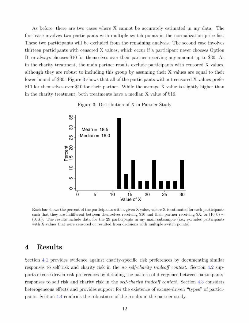
As before, there are two cases where X cannot be accurately estimated in my data. The

first case involves two participants with multiple switch points in the normalization price list.

These two participants will be excluded from the remaining analysis. The second case involves

thirteen participants with censored X values, which occur if a participant never chooses Option

B, or always chooses $10 for themselves over their partner receiving any amount up to $30. As

in the charity treatment, the main partner results exclude participants with censored X values,

although they are robust to including this group by assuming their X values are equal to their

lower bound of $30. Figure 3 shows that all of the participants without censored X values prefer

$10 for themselves over $10 for their partner. While the average X value is slightly higher than

in the charity treatment, both treatments have a median X value of $16.

Figure 3: Distribution of X in Partner Study

Mean = 18.5Median = 16.0

05

1015

2025

3035

Perc

ent

0 5 10 15 20 25 30Value of X

Each bar shows the percent of the participants with a given X value, where X is estimated for each participantssuch that they are indifferent between themselves receiving $10 and their partner receiving $X, or (10, 0) ∼(0, X). The results include data for the 29 participants in my main subsample (i.e., excludes participantswith X values that were censored or resulted from decisions with multiple switch points).

4 Results

Section 4.1 provides evidence against charity-specific risk preferences by documenting similar

responses to self risk and charity risk in the no self-charity tradeoff context. Section 4.2 sup-

ports excuse-driven risk preferences by detailing the pattern of divergence between participants’

responses to self risk and charity risk in the self-charity tradeoff context. Section 4.3 considers

heterogeneous effects and provides support for the existence of excuse-driven “types” of partici-

pants. Section 4.4 confirms the robustness of the results in the partner study.

12

4.1 Evidence against Charity-Specific Risk Preferences

The left panel of Figure 1 plots the self lottery and charity lottery valuations in the no self-charity

tradeoff context. With respect to participants’ valuations of self lotteries, they appear more risk

seeking with low probabilities (high risk) and risk averse with high probabilities (low risk). The

corresponding inverse-S pattern of valuations as a function of risk is a standard empirical finding

and replicates results from previous studies on risk. For instance, as shown in Appendix Figure

B.1, estimates of cumulative prospect theory parameters for the self lottery data are very similar

to previous studies.18

With respect to the comparison of responses to risk in self and charity payoffs, Appendix

Tables B.1 and B.2 confirm that the differences between valuations for charity lotteries and self

lotteries are not statistically different on average nor do they exceed more than a few percentage

points at any given probability level. These results also hold on a decision level; when considering

an individuals’ self and charity lottery valuations for a given probability, 42% are exactly the

same, and 83% differ by no more than ten percentage points.

4.2 Evidence for Excuse-Driven Risk Preferences

The right panel of Figure 1 plots the self lottery and charity lottery valuations in the self-charity

tradeoff context. Participants’ responses to charity risk and self risk now diverge by fifteen

percentage points on average. Appendix Tables B.3 and B.4 confirm this difference overall and

at the various probability levels. These results also hold on a decision level; when considering an

individuals’ self and charity lottery valuations for a given risk level, 78% are not the same, and

54% differ by more than ten percentage points.

To show that the observed divergence is consistent with excuse-driven risk preferences, con-

sider the difference-in-differences estimates from Equation 2. The dependent variable Yli is an

individual i’s valuation of a particular lottery l. While the coefficient on charity li captures

whether or not there are significant differences between charity and self lottery valuations in the

no self-charity tradeoff context, the coefficients on tradeoff li and charity*tradeoff li indicate the

extent to which there are excuse-driven risk preferences.

Yli = β0 + β1charityli + β2tradeoffli + β3charity*tradeoffli

+

(∑P

λP +∑i

µi

)+ εli (2)

where

18This observed pattern is more broadly consistent with models that allow for curvature via probability weight-ing functions (Prelec, 1998) or utility functions that are concave and convex over different ranges (Holt and Laury,2002).

13

Yli ≡ valuation of a lottery l (as a % of corresponding riskless lottery valuation)

charityli ≡ indicator for charity lottery

tradeoffli ≡ indicator for lottery being elicited in self-charity tradeoff context

charity*tradeoffli ≡ interaction variable of charity li and tradeoff li

λP ≡ probability fixed effect, P ∈ {0.95, 0.9, 0.75, 0.5, 0.25, 0.1 } (P=0.05 excluded)

µi ≡ individual fixed effect (individual i = 1 excluded)

Column 1 of Table 2 displays the corresponding regression results with no controls. To begin,

note that the coefficient on charity li is not statistically different than zero, consistent with the

lack of evidence for charity-specific risk preferences. However, the coefficient on tradeoff li shows

that participants’ self lottery valuations are about five percentage points higher on average in the

self-charity tradeoff context. Participants appear to overweight the possibility that self lotteries

yield non-zero-dollar payoffs, using it as an excuse to choose self lotteries over charity certain-

amounts more often than their non-excuse-driven risk preferences would imply. Additionally, the

sum of the coefficients on tradeoff li and charity*tradeoff li shows that participants’ charity lottery

valuations are about ten percentage points lower in the self-charity tradeoff context. Participants

appear to overweight the possibility that charity lotteries yield zero-dollar payoffs, using it as

an excuse to choose self certain-amounts over charity lotteries more often than their non-excuse-

driven risk preferences would imply.

Columns 2 - 4 confirm the robustness of the results to the inclusion of individual fixed effects

regardless of whether or not observations or participants with multiple switch points are excluded,

and Column 5 finds similar results with probability fixed effects. Column 6 shows that the results

hold with interval regressions, where the dependent variables are the upper and lower bounds of

the lottery valuations, as opposed to the midpoint of the range implied by participants’ price lists

decisions. While Columns 1 - 6 exclude participants with censored values of X, Column 7 shows

that the results are even larger when considering Tobit regressions that include participants with

censored values of X - i.e., individuals who are never willing to give up $10 for themselves in

exchange for the charity receiving any certain amount up to $30. As these individuals could

be considered the most selfish in this study, this larger finding could in part result from more

selfish individuals being more excuse-driven. The possibility for such heterogeneous effects, or

excuse-driven types of individuals, is further explored in the next section.

These results show that participants appear to use risk, regardless of whether it is charity

risk or self risk, as an excuse not to give. While the charity risk results may be more similar to

typical charitable giving decisions, the self risk results highlight a key advantage of the laboratory

environment as they serve as an useful robustness check of excuse-driven risk preferences. For

instance, contrary to the study instructions and the adhered policy of no deception in the Stanford

14

Table 2: Lottery Valuations

Regression: Ordinary Least Squares Interval TobitDV: Yl Y lower

l , YlY upperl

1 2 3 4 5 6 7charity 0.06 0.06 0.25 -0.44 0.06 0.23 1.30

(0.82) (0.82) (0.88) (0.83) (0.82) (0.87) (0.80)

tradeoff 5.30∗∗ 5.30∗∗ 5.58∗∗∗ 4.94∗∗ 5.30∗∗ 6.81∗∗∗ 27.50∗∗∗

(2.02) (2.02) (2.04) (2.21) (2.02) (2.31) (3.59)

charity*tradeoff -15.09∗∗∗ -15.09∗∗∗ -15.69∗∗∗ -14.51∗∗∗ -15.09∗∗∗ -16.53∗∗∗ -47.44∗∗∗

(3.40) (3.40) (3.50) (3.81) (3.41) (3.77) (5.29)

I(P = 0.95) 70.38∗∗∗

(1.87)

I(P = 0.90) 66.32∗∗∗

(1.76)

I(P = 0.75) 54.67∗∗∗

(1.46)

I(P = 0.50) 36.44∗∗∗

(1.18)

I(P = 0.25) 18.14∗∗∗

(1.09)

I(P = 0.10) 6.01∗∗∗

(0.63)

Constant 51.79∗∗∗ 51.79∗∗∗ 51.89∗∗∗ 51.85∗∗∗ 15.80∗∗∗ 51.83∗∗∗ 50.50∗∗∗

(0.96) (0.61) (0.63) (0.62) (1.36) (0.97) (0.80)Ind FE no yes yes yes no no noObs with MSP yes yes no no yes yes yesInd with MSP yes yes yes no yes yes yesCensored X no no no no no no yesObservations 1596 1596 1576 1400 1596 1596 2772Subjects 57 57 57 50 57 57 99

∗ p < 0.10, ∗∗ p < 0.05, ∗∗∗ p < 0.01. Standard errors are clustered at the individual level and shown inparentheses. The dependent variables are lottery valuations Yl - i.e., self-dollar valuations of self lotteries(Y s(P s)) or charity lotteries (Y s(P c)), and charity-dollar valuations of self lotteries (Y c(P s)) or charitylotteries (Y c(P c)). Valuations in self-dollars are scaled as percentages of $10, and valuations in charity-dollars are scaled as percentages of $Xi. The results are from regressions of Equation 2. Probability fixedeffects are shown when included, and “Ind FE” indicates whether or not individual fixed effects are included.“Obs with MSP” and “Ind with MSP” indicate whether or not observations with, or individuals that haveobservations with, multiple switch points are included. When observations involving multiple switch pointsare included, the first switch point is assumed. “Censored X” indicates whether or not participants withcensored X values are included. Note that 1 participant is always excluded because their X value resultedfrom decisions with multiple switch points.

15

Economics Research Laboratory, participants could believe that the experimenter will resolve

charity lotteries or distribute outcomes of charity lotteries in a manner biased against the charity

receiving its payoffs. Alternatively, participants may believe there is some additional risk in how

charities will use any donations they receive. Neither of these possibilities, however, can explain

why participants use self risk, not just charity risk, as an excuse not to give.

These results are robust to several other considerations as well. First, Appendix Tables

B.5 and B.6 confirm these results when separately looking at charity lottery valuations or self

lottery valuations. Second, Appendix Tables B.7 and B.8 provide evidence for excuse-driven risk

preferences when separately considering valuations elicited in self-dollars or charity-dollars as to

avoid the need to rescale valuations.19 Third, Appendix Table B.9 shows that the results are

robust to the order in which participants value charity lotteries or self lotteries, and the difference-

in-differences estimations ease other framing effects that may arise from the multiple price list

elicitations procedure.20 Fourth, similar findings are observed when considering decision level

results, as shown by the fraction of lottery valuations that fall below or exceed their expected

value in Appendix Figure B.2.

4.3 Evidence for Excuse-Driven Types of Participants

This section investigates the possibility of excuse-driven “types” of participants.21 Documenting

the existence of such types may help to unify the literature on excuse-driven behavior and to

limit the scope for non-excuse-driven explanations.

To begin, it is useful to note that there is an individual-level of consistency in excuse-driven

behavior across lottery valuations: participants who appear to use self risk as an excuse not to

give, by acting less averse to self risk in the self-charity tradeoff context, also appear to use charity

risk as an excuse not to give, by acting more averse to charity risk in the self-charity tradeoff

context.22 On one extreme, Figure 4 displays the valuations for a participant without excuse-

driven risk preferences: this participant always responds to self risk and charity risk in the same

19By only comparing valuations in self dollars to each other, or only comparing valuations in charity dollarsto each other, rescaling of valuations is not needed but I still find evidence for excuse-driven risk preferences.For self-dollar valuations, excuse-driven risk preferences are only relevant for the charity lotteries and wouldimply lower valuations for charity lotteries, as confirmed in Appendix Table B.7. For charity-dollar valuations,excuse-driven risk preferences are only relevant for self lotteries and would imply higher self lottery valuations,as confirmed in Appendix Table B.8.

20For instance, Castillo and Eil (2014) show that multiple price lists can cause people to act more or less averseto risk depending on the status quo, such as the fixed option in a price list. While participants may act less averseto risk since this study always fixed the risky payoff in Option A, such a level effect would be accounted for inthe difference-in-differences estimations.

21Previous literature that considers whether there exists “giving types” includes De Oliveira et al. (2011);Carpenter and Myers (2010).

22Consider the difference in a participant’s valuations of a lottery in the no self-charity tradeoff context andself-charity tradeoff context to indicate the extent to which their valuation of that lottery is self-serving. Thereis a strong positive rank correlation across nearly all pairwise comparisons of these differences.

16

manner across both contexts. By contrast, Figure 5 displays valuations for a participant with

clear excuse-driven risk preferences: this participant almost always acts less averse to self risk

and more averse to charity risk in the self-charity tradeoff context. The majority of participants,

without censored X values, appear to similarly exhibit excuse-driven risk preferences to varying

degrees: for 65% of the participants, the average difference in their lottery valuations across

contexts is in a self-serving direction that ranges from just under 1 to 42 percentage points.

Figure 4: Example Participant without Excuse-Driven Risk Preferences

Valuations ofCharity Lotteries

010

2030

4050

6070

8090

100

Valu

atio

n as

% o

f Ris

kles

s Lo

ttery

0 .1 .2 .3 .4 .5 .6 .7 .8 .9 1Probability P of Non-Zero Payment

No Self-Charity Tradeoff

Self-Charity Tradeoff

Expected Value

Valuations ofSelf Lotteries

010

2030

4050

6070

8090

100

Valu

atio

n as

% o

f Ris

kles

s Lo

ttery

0 .1 .2 .3 .4 .5 .6 .7 .8 .9 1Probability P of Non-Zero Payment

No Self-Charity Tradeoff

Self-Charity Tradeoff

Expected Value

In the left panel, the no self-charity tradeoff data indicate the charity-dollar valuations of charity lotteries,Y c(P c); the self-charity tradeoff data indicate the self-dollar valuations of charity lotteries, Y s(P c). In theright panel, the no self-charity tradeoff data indicate the self-dollar valuations of self lotteries, Y s(P s); theself-charity tradeoff data indicate the charity-dollar valuations of self lotteries, Y c(P s). Valuations in self-dollars are scaled as percentages of $10, and valuations in charity-dollars are scaled as percentages of $Xi.The Expected Value line indicates the expected value for a lottery given the probability P .

In addition to an individual-level consistency across lottery valuations, selfish participants

may be more likely to exhibit excuse-driven risk preferences. In this study, participants’ level of

selfishness is indicated by their X values – i.e., how much does the charity have to receive such

that they are willing to give up $10 for themselves. To consider whether participants’ X values

correspond with the extent of their excuse-driven behavior, I interact the main treatment effects

with (X − X), where X is the average X value among the participants. As shown in Column

2 of Table 4, participants with higher X values have a significantly larger tendency to exhibit

excuse-driven risk preferences. A one dollar increase in a participant’s X value corresponds with,

in self-charity tradeoff context, a $1.11 increase in self lottery valuations and a $0.45 decrease in

their charity lottery valuations, on average.

To consider an arguably more demanding test for excuse-driven types of participants, I ex-

amine whether excuse-driven risk preferences in lottery valuations correlate with excuse-driven

behavior in a separate task that replicates a “moral wiggle room” task developed in Dana et al.

(2007).23 The moral wiggle room task involves two important features. First, behavior in this

23The moral wiggle room task in my study closely follows two treatments from Dana et al. (2007) - i.e., their

17

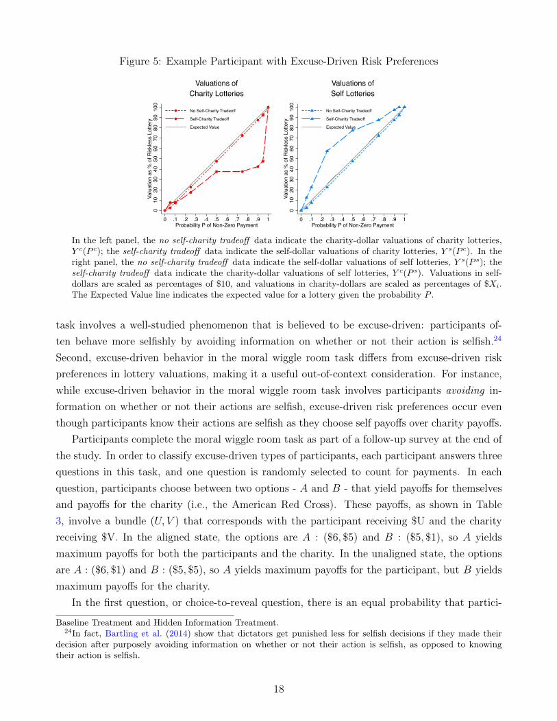
Figure 5: Example Participant with Excuse-Driven Risk Preferences

Valuations ofCharity Lotteries

010

2030

4050

6070

8090

100

Valu

atio

n as

% o

f Ris

kles

s Lo

ttery

0 .1 .2 .3 .4 .5 .6 .7 .8 .9 1Probability P of Non-Zero Payment

No Self-Charity Tradeoff

Self-Charity Tradeoff

Expected Value

Valuations ofSelf Lotteries

010

2030

4050

6070

8090

100

Valu

atio

n as

% o

f Ris

kles

s Lo

ttery

0 .1 .2 .3 .4 .5 .6 .7 .8 .9 1Probability P of Non-Zero Payment

No Self-Charity Tradeoff

Self-Charity Tradeoff

Expected Value

In the left panel, the no self-charity tradeoff data indicate the charity-dollar valuations of charity lotteries,Y c(P c); the self-charity tradeoff data indicate the self-dollar valuations of charity lotteries, Y s(P c). In theright panel, the no self-charity tradeoff data indicate the self-dollar valuations of self lotteries, Y s(P s); theself-charity tradeoff data indicate the charity-dollar valuations of self lotteries, Y c(P s). Valuations in self-dollars are scaled as percentages of $10, and valuations in charity-dollars are scaled as percentages of $Xi.The Expected Value line indicates the expected value for a lottery given the probability P .

task involves a well-studied phenomenon that is believed to be excuse-driven: participants of-

ten behave more selfishly by avoiding information on whether or not their action is selfish.24

Second, excuse-driven behavior in the moral wiggle room task differs from excuse-driven risk

preferences in lottery valuations, making it a useful out-of-context consideration. For instance,

while excuse-driven behavior in the moral wiggle room task involves participants avoiding in-

formation on whether or not their actions are selfish, excuse-driven risk preferences occur even

though participants know their actions are selfish as they choose self payoffs over charity payoffs.

Participants complete the moral wiggle room task as part of a follow-up survey at the end of

the study. In order to classify excuse-driven types of participants, each participant answers three

questions in this task, and one question is randomly selected to count for payments. In each

question, participants choose between two options - A and B - that yield payoffs for themselves

and payoffs for the charity (i.e., the American Red Cross). These payoffs, as shown in Table

3, involve a bundle (U, V ) that corresponds with the participant receiving $U and the charity

receiving $V. In the aligned state, the options are A : ($6, $5) and B : ($5, $1), so A yields

maximum payoffs for both the participants and the charity. In the unaligned state, the options

are A : ($6, $1) and B : ($5, $5), so A yields maximum payoffs for the participant, but B yields

maximum payoffs for the charity.

In the first question, or choice-to-reveal question, there is an equal probability that partici-

Baseline Treatment and Hidden Information Treatment.24In fact, Bartling et al. (2014) show that dictators get punished less for selfish decisions if they made their

decision after purposely avoiding information on whether or not their action is selfish, as opposed to knowingtheir action is selfish.

18

pants face payoffs in the unaligned state or in the aligned state. While participants are not told

which state they are in, they may reveal their state, for free, before choosing between A and B.

Choosing to reveal their state allows participants to ensure their preferred payoffs for themselves

and the charity. However, excuse-driven participants in the moral wiggle room task may choose

not to reveal their state; in doing so, they can then choose A without knowing whether or not A

is selfish. Studies documenting excuse-driven behavior in the moral wiggle room task typically

document such avoidance leading to an increase in overall selfish behavior.25

In the second question, or revealed-unaligned-state question, participants know they are in

the unaligned state and must choose between A and B. In this case, choosing A is selfish since

it results in lower charity payoffs in exchange for higher self payoffs.

In the third question, or revealed-aligned-state question, participants know they are in the

aligned state, and then must choose between A and B. In this case, choosing A is not selfish as

it yields the highest payoffs for both the participants and the charity.

Table 3: Moral Wiggle Room Payoffs

Unaligned State Aligned StateA (6,1) (6,5)

B (5,5) (5,1)

The bundle (U, V ) corresponds with theparticipant receiving $U and the charityreceiving $V.

While the aggregate results detailed in Appendix C provide evidence for excuse-driven be-

havior in the moral wiggle room task, I turn to individual level results to classify participants

according to their behavior in the moral wiggle room task. Aside from one participant (out

of the one-hundred), all participants are classified into one of the following three categories.26

First, 44% of the participants are selfish-types as they choose the selfish option A in the revealed-

unaligned-state question. These participants also choose the (potentially) selfish option A in the

choice-to-reveal question. Second, 35% of the participants are generous-types as they choose

the fair option B in the revealed-unaligned-state, and indicate that they place some value on

the charity payoffs in the choice-to-reveal question by choosing to reveal their state. Note that

conditional on participants revealing their state in the choice-to-reveal question, I do not classify

them according to their decision after the revelation; while I could classify whether participants

25In Dana et al. (2007), when their participants know they are in the unaligned state, only 26% chose theselfish option A. However, when their participants could choose whether or not to reveal their state, 63% of theirparticipants in the unaligned state chose the selfish option A. Dana et al. (2007) explain this behavior by pointingto moral wiggle room, as half of their participants chose not to reveal their state, and among that half, 100%choose the selfish option A.

26The one unclassified participant chose B in the choice-to-reveal state without revealing their state first. Thischoice guarantees themselves their lowest payoff and may or may not give the charity its lowest payoff as well.

19

who learn they are in the unaligned-state as choosing the selfish option or not, I could not make

the same classification for participants who learn they are in the aligned-state. Third, 20% of the

participants are wiggler-types as they choose the fair option B in the revealed-unaligned-state,

but instead choose the potentially selfish option A in the choice-to-reveal question after choosing

not to reveal their state. That is, wiggler-types, or those susceptible to excuse-driven behavior

in the moral wiggle room task, only choose the potentially selfish option when they can and

do avoid free information on whether or not their choice is selfish. Among participants in my

main subsample (as relevant later in Table 4), the relative representation of types changes to

selfish-types (23%), generous-types (51%), and wiggler-types (25%).27

Both generous-types and wiggler-types choose the fair option B in the revealed-unaligned-

state question. Wiggler-types, however, avoid learning their state in the choice-to-reveal question

and choose the potentially selfish option A. If there is an individual-level of consistency in excuse-

driven behavior out-of-sample, then wiggler-types should be more likely to exhibit excuse-driven

risk preferences than generous-types.

As shown in the third column of Table 4, wiggler-types are more likely to exhibit excuse-

driven risk preferences, particularly with respect to using charity risk as an excuse not to give.28

In self-charity tradeoff context, they have significantly lower charity lottery valuations and quali-

tatively, although not significantly, higher self lottery valuations. Similar results may be expected

for selfish-types, particularly in light of the earlier finding shown in Column 2: individuals with

higher X values show a greater tendency to exhibit excuse-driven behavior. While qualitatively

consistent with this possibility, the binary classification of selfish-types does not significantly

correspond with more excuse-driven behavior. This may in part be explained by the somewhat

surprising finding of an insignificant correlation between participants’ values of X and classifica-

tions as selfish-types. There is also an insignificant correlation between participants’ values of

X and classifications as wiggler-types, which suggests that these two characteristics may inde-

pendently be important predictors of excuse-driven behavior. The fourth column of Table 4 in

fact confirms that the same results hold even when there are interactions of the treatment effects

with (X− X), wiggler-types, and selfish-types. As a matter of interest, no significant interaction

effects are observed when the treatment effects are instead interacted with an indicator for a

participant’s sex or stated degree of how favorably they view the American Red Cross.

27Relatively fewer selfish-types results from my main subsample excluding participants with censored X values,who also have more selfish decisions in the moral wiggle room task.

28The results are robust to excluding the one unclassified participant from the moral wiggle room task as well.

20

Table 4: Examining Heterogeneous Effects

Regression: Ordinary Least SquaresDV: Yl

1 2 3 4charity 0.06 0.06 0.10 0.09

(0.82) (0.80) (1.26) (1.23)

tradeoff 5.30∗∗ 5.30∗∗∗ 3.15 3.15(2.02) (1.82) (2.83) (2.38)

charity*tradeoff -15.09∗∗∗ -15.09∗∗∗ -9.02∗ -9.02∗∗

(3.40) (3.18) (4.55) (3.90)

(X − X) -0.11 -0.11(0.13) (0.13)

charity* (X − X) 0.26∗ 0.26∗

(0.13) (0.13)

tradeoff* (X − X) 1.11∗∗∗ 1.11∗∗∗

(0.31) (0.31)

charity*tradeoff* (X − X) -1.56∗∗∗ -1.56∗∗

(0.57) (0.59)

wiggler -0.62 -0.62(2.17) (2.21)

charity*wiggler 0.90 0.89(1.65) (1.60)

tradeoff*wiggler 4.47 4.45(4.54) (3.99)

charity*tradeoff*wiggler -13.48∗∗ -13.45∗∗

(6.46) (5.28)

selfish 2.68 2.67(2.54) (2.49)

charity*selfish -1.14 -1.13(2.17) (2.10)

tradeoff*selfish 4.59 4.63(5.25) (5.09)

charity*tradeoff*selfish -12.10 -12.16(9.78) (10.04)

Constant 51.79∗∗∗ 51.79∗∗∗ 51.33∗∗∗ 51.33∗∗∗

(0.96) (0.96) (1.30) (1.30)Observations 1596 1596 1596 1596Subjects 57 57 57 57

∗ p < 0.10, ∗∗ p < 0.05, ∗∗∗ p < 0.01. Standard errors are clustered at the individual level and shown in parentheses.The dependent variables are lottery valuations Yl - i.e., self-dollar valuations of self lotteries (Y s(P s)) or charitylotteries (Y s(P c)), and charity-dollar valuations of self lotteries (Y c(P s)) or charity lotteries (Y c(P c)). Valuationsin self-dollars are scaled as percentages of $10, and valuations in charity-dollars are scaled as percentages of $Xi.The results are from regressions of Equation 2 modified to include the shown interactions. (X−X) is a participant’sX minus the average X. selfish is an indicator for choosing A in the revealed-unaligned state. wiggler is an indicatorfor choosing B in the revealed-unaligned-state but A in the choice-to-reveal question after choosing not to revealtheir state. For observations involving multiple switch points, the first switch point is assumed. Participants withcensored X values or X values that resulted from decisions with multiple switch points are excluded.

21

4.4 Replication of Results in Partner Study

In the partner study, payoffs benefit another participant in the lab as opposed to the charity.

Results may therefore differ from the above discussed charity study due to several reasons –

perhaps most notably if excuse-driven behavior is only relevant to charitable giving and not

prosocial behavior more broadly. Additionally, while the partner version eliminates differences

in how payments to oneself and others are being distributed, it also introduces role-uncertainty

(Iriberri and Rey-Biel, 2011) as participants do not know if their decisions or their partners’

decisions will be implemented for payment.

As shown in Figure 6 and Appendix Table B.10, evidence for excuse-driven risk preferences

is similar, and if anything, larger in the partner study. In the no self-partner tradeoff context,

participants respond very similarly to risk. By contrast, in the self-partner tradeoff context,

participants act more averse to partner risk and less averse to self risk. Table 5 provides evidence

for excuse-driven risk preferences when pooling data from the charity study and partner study,

and as shown in Column 2, finds qualitatively but not significantly larger evidence for excuse-

driven risk preferences in the partner study. Moreover, as shown in Columns 3 and 4 of Table

5, it remains true that participants with higher values of X are more likely to exhibit a stronger

tendency for excuse-driven behavior.

Figure 6: Lottery Valuations in Partner Study

No Self-Partner Tradeoff

010

2030

4050

6070

8090

100

Valu

atio

n as

% o

f Ris

kles

s Lo

ttery

0 .1 .2 .3 .4 .5 .6 .7 .8 .9 1Probability P of Non-Zero Payment

Self Lottery

Partner Lottery

Expected Value

Self-Partner Tradeoff

010

2030

4050

6070

8090

100

Valu

atio

n as

% o

f Ris

kles

s Lo

ttery

0 .1 .2 .3 .4 .5 .6 .7 .8 .9 1Probability P of Non-Zero Payment

Self Lottery

Partner Lottery

Expected Value

In the left panel, the estimates are valuations in the no self-partner tradeoff context : the self lottery dataindicate the self-dollar valuations of self lotteries, Y s(P s); the partner lottery data indicate the partner dollarvaluations of partner lotteries, Y p(P p). In the right panel, the estimates are valuations in the self-partnertradeoff context : the self lottery data indicate the partner dollar valuations of self lotteries, Y p(P s); thepartner lottery data indicate the self-dollar valuations of partner lotteries, Y s(P p). Valuations in self-dollarsare scaled as percentages of $10, and valuations in partner-dollars are scaled as percentages of $X. TheExpected Value line indicates the expected value for a lottery given the probability P . The results includedata for the 29 participants in my main subsample (i.e., excludes participants with X values that were censoredor resulted from decisions with multiple switch points). For observations involving multiple switch points,the first switch point is assumed.

22

Table 5: Lottery Valuations in Charity Study and Partner Study

Regression: Ordinary Least SquaresDV: Yl

1 2 3 4other 0.68 0.06 0.68 0.10

(0.69) (0.82) (0.69) (0.83)

tradeoff 6.94∗∗∗ 5.30∗∗ 6.94∗∗∗ 5.77∗∗∗

(1.77) (2.01) (1.59) (1.85)

other*tradeoff -17.60∗∗∗ -15.09∗∗∗ -17.60∗∗∗ -15.80∗∗∗

(2.87) (3.39) (2.62) (3.21)

partner-study -2.10 -2.18(1.70) (1.70)

other*partner-study 1.84 1.72(1.47) (1.54)

tradeoff*partner-study 4.87 3.48(3.92) (3.49)

other*tradeoff*partner-study -7.44 -5.34(6.20) (5.56)

(X − X) 0.05 0.07(0.10) (0.11)

other* (X − X) 0.11 0.10(0.10) (0.10)

tradeoff* (X − X) 1.17∗∗∗ 1.14∗∗∗

(0.27) (0.27)

other*tradeoff* (X − X) -1.77∗∗∗ -1.73∗∗∗

(0.45) (0.44)

Constant 51.08∗∗∗ 51.79∗∗∗ 51.08∗∗∗ 51.82∗∗∗

(0.80) (0.96) (0.80) (0.96)Observations 2408 2408 2408 2408Subjects 86 86 86 86

∗ p < 0.10, ∗∗ p < 0.05, ∗∗∗ p < 0.01. Standard errors are clustered at the individuallevel and shown in parentheses. The dependent variables are lottery valuationsYl - i.e., in the charity-study: self-dollar valuations of self lotteries (Y s(P s)) orcharity lotteries (Y s(P c)), and charity-dollar valuations of self lotteries (Y c(P s))or charity lotteries (Y c(P c)); and in the partner-study: self-dollar valuations of selflotteries (Y s(P s)) or partner lotteries (Y s(P p)), and partner-dollar valuations of selflotteries (Y p(P s)) or partner lotteries (Y p(P p)). Valuations in self-dollars are scaledas percentages of $10, and valuations in charity-dollars or partner-dollars are scaledas percentages of $X. The results are from regressions of Equation 2 modified toinclude the shown interactions and modified such that charity is replaced by other(an indicator for charity or partner). (X−X) is a participant’s X minus the averageX. partner-study is an indicator for the partner study. For observations involvingmultiple switch points, the first switch point is assumed. Participants with censoredX values or X values that resulted from decisions with multiple switch points areexcluded.

23

5 Conclusion

In examining how individuals respond to risk in charitable giving decisions, this study documents

a novel pattern of behavior. When participants cannot use risk as an excuse not to give, in the

no self-charity tradeoff context, they respond very similarly to risk in self lotteries and charity

lotteries. However, when participants may use risk as an excuse not to give, in the self-charity

tradeoff context, they act more averse to charity risk and less averse to self risk.

This excuse-driven interpretation is bolstered by documenting an individual level of consis-

tency in excuse-driven behavior. Participants’ extent of excuse-driven risk preferences is strongly

correlated with their level of selfishness, and engagement in excuse-driven behavior in a moral

wiggle room task, as developed in Dana et al. (2007). In an additional study, excuse-driven

risk preferences are similarly strong when participants decide between payoffs for themselves and

payoffs for another study participant.

As the observed excuse-driven risk preferences yield violations of transitivity29, these results

may be most easily rationalized with a menu-dependent model that allows for different responses

to risk depending on whether or not the environment permits excuses.30 Another possibility

may involve fleshing out models where individuals infer their type based off of their own past

behavior, but their inference about their prosocial tendencies is less informative in the presence

of risk.31

Other fruitful avenues for future work may involve testing related policy implications. The

evidence for excuse-driven types of individuals, in particular, indicates that charities may be able

to exploit the heterogeneity in the types of potential donors when determining how to target

fundraising requests. Potential implications for nonprofit organizations may also relate to other

avenues for excuse-driven behavior in charitable giving; for instance, Exley (2015) demonstrates

how individuals may use lower charity performance metrics as excuses not to give.

29 For instance, 72% of participants have lower self-dollar valuations of charity lotteries, Y s(0.95c), than compa-rable self-dollar valuations of self lotteries Y s(0.95s), which implies 0.95c ≺ 0.95s. By contrast, 63% of participantsdo not have lower charity-dollar valuations of charity lotteries Y c(P c) than comparable charity-dollar valuationsof self lotteries Y c(0.95s), which implies 0.95c � 0.95s. Assuming transitivity yields this particular preferencereversal for 42% of the participants. A similarly high level of preference reversals exist for lottery valuations thatexhibit the largest amount of excuse-driven risk preferences.

30One possibility may involve temptation models, such as Gul and Pesendorfer (2001), if “not giving” is classifiedas a tempting good. Interestingly though, previous literature, such as Andreoni et al. (2011), also discusses how“giving” may be considered a tempting good.

31That is, if individuals update both on their prosocial and risk preferences, then the strength of either signalmay be reduced, such as when individuals may update on both their greedy and prosocial preferences in Benabouand Tirole (2006).

24

References

Andersson, Ola, Hakan J Holm, Jean-Robert Tyran, and Erik Wengstrom. 2013.

“Risking other people’s money: Experimental evidence on bonus schemes, competition, and

altruism.” IFN Working Paper.

Andersson, Ola, Hakan J Holm, Jean-Robert Tyran, and Erik Wengstrom. 2014.

“Deciding for others reduces loss aversion.” Management Science.

Andreoni, James. 1989. “Giving with Impure Altruism: Applications to Charity and Ricardian

Equivalence.” The Journal of Political Economy, 1447–1458.

Andreoni, James. 1990. “Impure Altruism and Donations to Public Goods: A Theory of

Warm-Glow Giving.” The Economic Journal, 100(401): 464–477.

Andreoni, James. 2006. “Chapter 18 Philanthropy.” In Applications. Vol. 2 of Handbook on the

Economics of Giving, Reciprocity and Altruism, , ed. Serge-Christophe Kolm and Jean Mercier

Ythier, 1201 – 1269. Elsevier.

Andreoni, James, and B. Douglas Bernheim. 2009. “Social Image and the 50–50 Norm: A

Theoretical and Experimental Analysis of Audience Effects.” Econometrica, 77(5): 1607–1636.

Andreoni, James, and Charles Sprenger. 2011. “Uncertainty Equivalents: Testing the

Limits of the Independence Axiom.” NBER Working Paper No. 17342.

Andreoni, James, and Justin M. Rao. 2011. “The power of asking: How communication

affects selfishness, empathy, and altruism.” Journal of Public Economics, 95: 513–520.

Andreoni, James, and Ragan Petrie. 2004. “Public goods experiments without confiden-

tiality: a glimpse into fund-raising.” Journal of Public Economics, 88: 1605–1623.

Andreoni, James, Justin M. Rao, and Hannah Trachtman. 2011. “Avoiding the ask:

A field experiment on altruism, empathy, and charitable giving.” NBER Working Paper No.

17648.

Ariely, Dan, Anat Bracha, and Stephan Meier. 2009. “Doing Good or Doing Well? Image

Motivation and Monetary Incentives in Behaving Prosocially.” American Economic Review,

99(1): 544–555.

Azrielli, Yaron, Christopher P. Chambers, and Paul J. Healey. 2014. “Incentives in

Experiments: A Theoretical Analysis.” Working Paper.

Bartling, Bjorn, and Urs Fischbacher. 2012. “Shifting the Blame: On Delegation and

Responsibility.” Review of Economic Studies, 79(1): 67–87.

25

Bartling, Bjorn, Florian Engl, and Roberto A. Weber. 2014. “Does willful ignorance

deflect punishment? – An experimental study.” European Economic Review, 70(0): 512 – 524.

Batista, Catia, Dan Silverman, and Dean Yang. 2015. “Directed Giving: Evidence from

an Inter-Household Transfer Experiment.” Journal of Economic Behavior & Organization.

Benabou, Roland, and Jean Tirole. 2006. “Incentives and Prosocial Behavior.” American

Economic Review, 96(5): 1652–1678.

Bernheim, B. Douglas, and Christine L. Exley. 2015. “Understanding Conformity: An

Experimental Investigation.” Working Paper.

Bolton, Gary E., and Axel Ockenfels. 2010. “Betrayal aversion: Evidence from brazil, china,

oman, switzerland, turkey, and the united states: Comment.” American Economic Review,

628–633.

Brennan, Geoffrey, Luis G. Gonzalez, Werner Guth, and M. Vittoria Levati. 2008.

“Attitudes toward private and collective risk in individual and strategic choice situations.”

Journal of Economic Behavior & Organization, 67(1): 253–262.

Broberg, Tomas, Tore Ellingsen, and Magnus Johannesson. 2007. “Is generosity invol-

untary?” Economics Letters, 94(1): 32–37.

Brock, J. Michelle, Andreas Lange, and Erkut Y. Ozbay. 2013. “Dictating the Risk:

Experimental Evidence on Giving in Risky Environments.” American Economic Review,

103(1): 415–437.

Brown, Alexander L., Jonathan Meer, and J. Forrest Williams. 2014. “Social Distance

and Quality Ratings in Charity Choice.” NBER Working Paper Series.

Carpenter, Jeffrey, and Caitlin Knowles Myers. 2010. “Why volunteer? Evidence on the

role of altruism, image, and incentives.” Journal of Public Economics, 94(11-12): 911 – 920.

Castillo, Marco, and David Eil. 2014. “Taring the Multiple Price List: Imperceptive Prefer-

ences and the Reversing of the Common Ratio Effect.” Working Paper.

Castillo, Marco, Ragan Petrie, and Clarence Wardell. 2014. “Fundraising through online

social networks: A field experiment on peer-to-peer solicitation.” Journal of Public Economcis,

29–35.

Chakravarty, Sujoy, Glenn W. Harrison, Ernan E. Haruvy, and E. Elisabet Rut-

strom. 2011. “Are you risk averse over other people’s money?” Southern Economic Journal,

77(4): 901–913.

26

Coffman, Lucas C. 2011. “Intermediation Reduces Punishment (and Reward).” American

Economic Journal: Microeconomics, 3(4): 1–30.

Dana, Jason, Daylian M. Cain, and Robyn M. Dawes. 2006. “What you don’t know won’t

hurt me: Costly (but quiet) exit in dictator games.” Organizational Behavior and Human

Decision Processes, 100: 193–201.

Dana, Jason, Roberto A. Weber, and Jason Xi Kuang. 2007. “Exploiting moral wig-

gle room: experiments demonstrating an illusory preference for fairness.” Economic Theory,

33(67–80).

DellaVigna, Stefano, John List, and Ulrike Malmendier. 2012. “Testing for Altruism and

Social Pressure in Charitable Giving.” Quarterly Journal of Economics, 127(1): 1–56.

De Oliveira, Angela, Rachel T.A Croson, and Catherine Eckel. 2011. “The giving type:

Identifying donors.” Journal of Public Economics, 95(5): 428–435.

Engel, Christoph. 2011. “Dictator games: a meta study.” Experimental Economics, 14(4): 583–

610.

Eriksen, Kristoffer, Ola Kvaløy, and Miguel Luzuriaga. 2014. “Risk-taking with Other

People’s Money.” Working Paper.

Exley, Christine L. 2014. “Incentives for Prosocial Behavior: The Role of Reputations.” Work-

ing Paper.

Exley, Christine L. 2015. “Using Charity Performance Metrics as an Excuse Not To Give.”

Working Paper.

Exley, Christine L., and Stephen J. Terry. 2015. “Wage Elasticities in Working and Vol-

unteering: The Role of Reference Points in a Laboratory Study.” Working Paper.

Falk, Armin, and Nora Szech. 2013. “Organizations, Diffused Pivotality and Immoral Out-

comes.” IZA Discussion Paper 7442.

Fong, Christina M., and Felix Oberholzer-Gee. 2011. “Truth in giving: Experimental

evidence on the welfare effects of informed giving to the poor.” Journal of Public Economics,

95: 436–444.

Gneezy, Uri, Elizabeth A. Keenan, and Ayelet Gneezy. 2014. “Avoiding overhead aversion

in charity.” Science, 346(6209): 632–635.

Grossman, Zachary. 2014. “Strategic ignorance and the robustness of social preferences.”

Management Science, 60(11): 2659–2665.

27

Gul, Faruk, and Wolfgang Pesendorfer. 2001. “Temptation and Self-Control.” Economet-

rica, 69(6): 1403–1435.

Guth, Werner M., Vittoria Levati, and Matteo Ploner. 2008. “On the social dimension

of time and risk preferences: An experimental study.” Economic Inquiry, 46(2): 261–272.

Haisley, Emily C., and Roberto A. Weber. 2010. “Self-serving interpretations of ambiguity

in other-regarding behavior.” Games and Economic Behavior, 68: 614–625.

Hamman, John R., George Loewenstein, and Roberto A. Weber. 2010. “Self-Interest

through Delegation: An Additional Rationale for the Principal-Agent Relationship.” American

Economic Review, 100(4): 1826–1846.

Harbaugh, William T. 1998a. “The Prestige Motive for Making Charitable Transfers.” The

American Economic Review, 88(2): pp. 277–282.

Harbaugh, William T. 1998b. “What do donations buy?: A model of philanthropy based on

prestige and warm glow.” Journal of Public Economics, 67(2): 269 – 284.

Holt, Charles, and Susan Laury. 2002. “Risk Aversion and Incentive Effects.” The American

Economic Review, 92(5): 1644– 1655.

Iriberri, Nagore, and Pedro Rey-Biel. 2011. “The role of role uncertainty in modified

dictator games.” Experimental Economics, 14(2): 160–180.

Karlan, Dean, and Daniel H. Wood. 2014. “The effect of effectiveness: donor response to aid

effectiveness in a direct mail fundraising experiment.” NBER Working Paper Series, Working

Paper 20047.

Konow, James. 2000. “Fair Shares: Accountability and Cognitive Dissonance in Allocation

Decisions.” The American Economic Review, 90(4): 1072–1092.

Krawczyk, Michal, and Fabrice Le Lec. 2010. “‘Give me a chance!’ An experiment in social

decision under risk.” Experimental Economics, 13(4): 500–511.

Lacetera, Nicola, and Mario Macis. 2010. “Social image concerns and prosocial behavior:

Field evidence from a nonlinear incentive scheme.” Journal of Economic Behavior and Orga-

nization, 76(2): 225 – 237.

Landry, Craig, Andreas Lange, John A. List, Michael K. Price, and Nicholas G.

Rupp. 2006. “Toward an understanding of the economics of charity: Evidence from a field

experiment.” The Quarterly Journal of Economics.

28

Lazear, Edward P., Ulrike Malmendier, and Roberto A. Weber. 2012. “Sorting in

experiments with application to social preferences.” American Economic Journal: Applied

Economics, 4(1): 136–163.

Linardi, Sera, and Margaret A. McConnell. 2011. “No excuses for good behavior: Volun-

teering and the social environment.” Journal of Public Economics, 95: 445–454.

Li, Sherry Xin, Catherine Eckel, Philip J. Grossman, and Tara Larson Brown. 2013.

“Who’s in Charge? Donor Targeting Enhances Voluntary Giving to Government.” Working

paper.

Meer, Jonathan. 2014. “Effects of the price of charitable giving: Evidence from an online

crowdfunding platform.” Journal of Economic Behavior & Organization, 103: 113–124.

Meier, Stephan, and Charles Sprenger. 2010. “Present-Biased Preferences and Credit Card

Borrowing.” American Economic Journal: Applied Economics, 2(1): 193–210.

Merritt, Anna C., Daniel A. Effron, and Benoıt Monin. 2010. “Moral Self-Licensing:

When Being Good Frees Us to Be Bad.” Social and Personality Psychology Compass, 4(5): 344–

357.

Niehaus, Paul. 2014. “A Theory of Good Intentions.” Working Paper.

Oberholzer-Gee, Felix, and Reiner Eichenberger. 2008. “Fairness in Extended Dictator

Game Experiments.” The B.E. Journal of Economic Analysis & Policy, 8(1).

Prelec, Drazen. 1998. “The Probability Weighting Function.” Econometrica, 66(3): 497–527.

Small, Deborah A., and George Loewenstein. 2003. “Helping a Victim or Helping the

Victim: Altruism and Identifiability.” Journal of Risk and Uncertainty, 26(1): 5–16.

Tversky, Amos, and Daniel Kahneman. 1992. “Advances in Prospect Theory: Cumulative

Representation of Uncertainty.” Journal of Risk and Uncertainty, 5: 297–323.

van der Weele, Joel J., Julija Kulisa, Michael Kosfeld, and Guido Friebel. 2014.

“Resisting Moral Wiggle Room: How Robust Is Reciprocal Behavior?” American Economic

Journal: Microeconomics, 6(3): 256–264.

Vesterlund, Lise. 2006. “Why do people give?” In The Nonprofit Sector: A Research Handbook,

2nd Edition. , ed. Walter W. Powell and Richard Steinberg, 568–87. New Haven, CT:Yale

University Press.

Yoruk, Baris K. 2013. “Charity Ratings.” Working Paper.

29

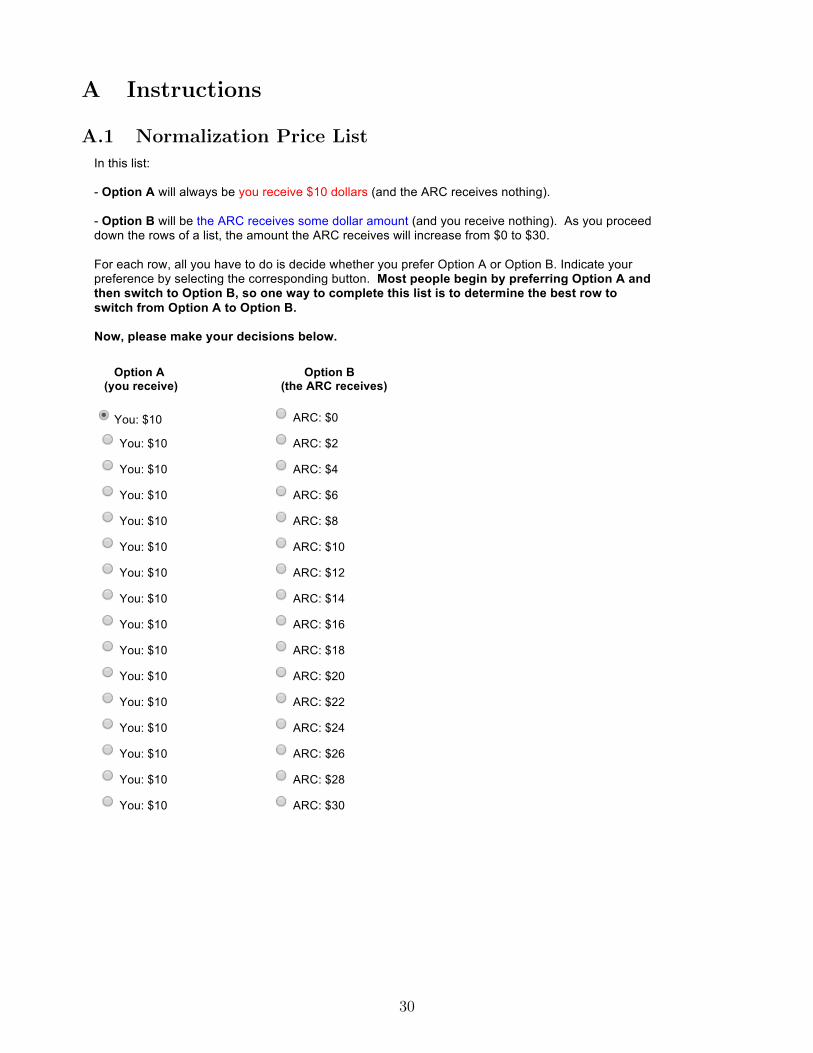
A Instructions

A.1 Normalization Price ListBlock 1, List 1 In this list: - Option A will always be you receive $10 dollars (and the ARC receives nothing). - Option B will be the ARC receives some dollar amount (and you receive nothing). As you proceed down the rows of a list, the amount the ARC receives will increase from $0 to $30. For each row, all you have to do is decide whether you prefer Option A or Option B. Indicate your preference by selecting the corresponding button. Most people begin by preferring Option A and then switch to Option B, so one way to complete this list is to determine the best row to switch from Option A to Option B. Now, please make your decisions below. Option A (you receive)

Option B (the ARC receives)

You: $10 ARC: $0

You: $10 ARC: $2

You: $10 ARC: $4

You: $10 ARC: $6

You: $10 ARC: $8

You: $10 ARC: $10

You: $10 ARC: $12

You: $10 ARC: $14

You: $10 ARC: $16

You: $10 ARC: $18

You: $10 ARC: $20

You: $10 ARC: $22

You: $10 ARC: $24

You: $10 ARC: $26

You: $10 ARC: $28

You: $10 ARC: $30

!!!!!

30

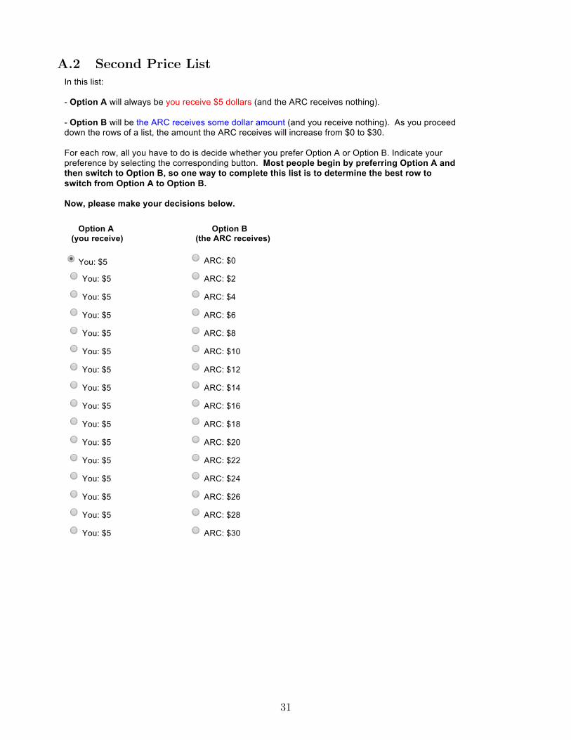
A.2 Second Price List Block 1, List 2 In this list: - Option A will always be you receive $5 dollars (and the ARC receives nothing). - Option B will be the ARC receives some dollar amount (and you receive nothing). As you proceed down the rows of a list, the amount the ARC receives will increase from $0 to $30. For each row, all you have to do is decide whether you prefer Option A or Option B. Indicate your preference by selecting the corresponding button. Most people begin by preferring Option A and then switch to Option B, so one way to complete this list is to determine the best row to switch from Option A to Option B. Now, please make your decisions below. Option A (you receive)

Option B (the ARC receives)

You: $5 ARC: $0

You: $5 ARC: $2

You: $5 ARC: $4

You: $5 ARC: $6

You: $5 ARC: $8

You: $5 ARC: $10

You: $5 ARC: $12

You: $5 ARC: $14

You: $5 ARC: $16

You: $5 ARC: $18

You: $5 ARC: $20

You: $5 ARC: $22

You: $5 ARC: $24

You: $5 ARC: $26

You: $5 ARC: $28

You: $5 ARC: $30

!!!

!!!!!

31

A.3 Valuation Price List: Example from Self Dollar Valuation of Self

Lottery, Y s(P s), BlockBlock 2, List 1

In this list: - Option A will always be you receive $10 dollars with probability 95%, and $0 otherwise (and the ARC receives nothing). - Option B will be you receive some dollar amount (and the ARC receives nothing). As you proceed down the rows of a list, the amount you receive will increase from $0 to $10. For each row, all you have to do is decide whether you prefer Option A or Option B. Indicate your preference by selecting the corresponding button. Most people begin by preferring Option A and then switch to Option B, so one way to complete this list is to determine the best row to switch from Option A to Option B. Now, please make your decisions below. Option A (you receive)

Option B (you)

You: $10 with probability 95%, and $0 otherwise You: $0

You: $10 with probability 95%, and $0 otherwise You: $0.50

You: $10 with probability 95%, and $0 otherwise You: $1

You: $10 with probability 95%, and $0 otherwise You: $1.50

You: $10 with probability 95%, and $0 otherwise You: $2

You: $10 with probability 95%, and $0 otherwise You: $2.50

You: $10 with probability 95%, and $0 otherwise You: $3

You: $10 with probability 95%, and $0 otherwise You: $3.50

You: $10 with probability 95%, and $0 otherwise You: $4

You: $10 with probability 95%, and $0 otherwise You: $4.50

You: $10 with probability 95%, and $0 otherwise You: $5

You: $10 with probability 95%, and $0 otherwise You: $5.50

You: $10 with probability 95%, and $0 otherwise You: $6

You: $10 with probability 95%, and $0 otherwise You: $6.50

You: $10 with probability 95%, and $0 otherwise You: $7

You: $10 with probability 95%, and $0 otherwise You: $7.50

You: $10 with probability 95%, and $0 otherwise You: $8

You: $10 with probability 95%, and $0 otherwise You: $8.50

You: $10 with probability 95%, and $0 otherwise You: $9

You: $10 with probability 95%, and $0 otherwise You: $9.50

You: $10 with probability 95%, and $0 otherwise You: $10

32

A.4 Valuation Price List: Example from Charity Dollar Valuation of

Charity Lottery, Y c(P c), BlockBlock 3, List 1

In this list: - Option A will always be the ARC receives $20 dollars with probability 95%, and $0 otherwise (and you receive nothing). - Option B will be the ARC receives some dollar amount (and you receive nothing). As you proceed down the rows of a list, the amount the ARC receives will increase from $0 to $20. For each row, all you have to do is decide whether you prefer Option A or Option B. Indicate your preference by selecting the corresponding button. Most people begin by preferring Option A and then switch to Option B, so one way to complete this list is to determine the best row to switch from Option A to Option B. Now, please make your decisions below. Option A (the ARC receives)

Option B (the ARC receives)

ARC: $20 with probability 95%, and $0 otherwise ARC: $0

ARC: $20 with probability 95%, and $0 otherwise ARC: $1

ARC: $20 with probability 95%, and $0 otherwise ARC: $2

ARC: $20 with probability 95%, and $0 otherwise ARC: $3

ARC: $20 with probability 95%, and $0 otherwise ARC: $4

ARC: $20 with probability 95%, and $0 otherwise ARC: $5

ARC: $20 with probability 95%, and $0 otherwise ARC: $6

ARC: $20 with probability 95%, and $0 otherwise ARC: $7

ARC: $20 with probability 95%, and $0 otherwise ARC: $8

ARC: $20 with probability 95%, and $0 otherwise ARC: $9

ARC: $20 with probability 95%, and $0 otherwise ARC: $10

ARC: $20 with probability 95%, and $0 otherwise ARC: $11

ARC: $20 with probability 95%, and $0 otherwise ARC: $12

ARC: $20 with probability 95%, and $0 otherwise ARC: $13

ARC: $20 with probability 95%, and $0 otherwise ARC: $14

ARC: $20 with probability 95%, and $0 otherwise ARC: $15

ARC: $20 with probability 95%, and $0 otherwise ARC: $16

ARC: $20 with probability 95%, and $0 otherwise ARC: $17

ARC: $20 with probability 95%, and $0 otherwise ARC: $18

ARC: $20 with probability 95%, and $0 otherwise ARC: $19

ARC: $20 with probability 95%, and $0 otherwise ARC: $20

33

A.5 Valuation Price List: Example from Self Dollar Valuation of

Charity Lottery, Y s(P c), BlockBlock 4, List 1

In this list: - Option A will always be the ARC receives $20 dollars with probability 95%, and $0 otherwise (and you receive nothing). - Option B will be you receive some dollar amount (and the ARC receives nothing). As you proceed down the rows of a list, the amount you receive will increase from $0 to $10. For each row, all you have to do is decide whether you prefer Option A or Option B. Indicate your preference by selecting the corresponding button. Most people begin by preferring Option A and then switch to Option B, so one way to complete this list is to determine the best row to switch from Option A to Option B. Now, please make your decisions below. Option A (the ARC receives)

Option B (you)

ARC: $20 with probability 95%, and $0 otherwise You: $0

ARC: $20 with probability 95%, and $0 otherwise You: $0.50

ARC: $20 with probability 95%, and $0 otherwise You: $1

ARC: $20 with probability 95%, and $0 otherwise You: $1.50

ARC: $20 with probability 95%, and $0 otherwise You: $2

ARC: $20 with probability 95%, and $0 otherwise You: $2.50

ARC: $20 with probability 95%, and $0 otherwise You: $3

ARC: $20 with probability 95%, and $0 otherwise You: $3.50

ARC: $20 with probability 95%, and $0 otherwise You: $4

ARC: $20 with probability 95%, and $0 otherwise You: $4.50

ARC: $20 with probability 95%, and $0 otherwise You: $5

ARC: $20 with probability 95%, and $0 otherwise You: $5.50

ARC: $20 with probability 95%, and $0 otherwise You: $6

ARC: $20 with probability 95%, and $0 otherwise You: $6.50

ARC: $20 with probability 95%, and $0 otherwise You: $7

ARC: $20 with probability 95%, and $0 otherwise You: $7.50

ARC: $20 with probability 95%, and $0 otherwise You: $7.50

ARC: $20 with probability 95%, and $0 otherwise You: $8

ARC: $20 with probability 95%, and $0 otherwise You: $8.50

ARC: $20 with probability 95%, and $0 otherwise You: $9

ARC: $20 with probability 95%, and $0 otherwise You: $9.50

ARC: $20 with probability 95%, and $0 otherwise You: $10

34

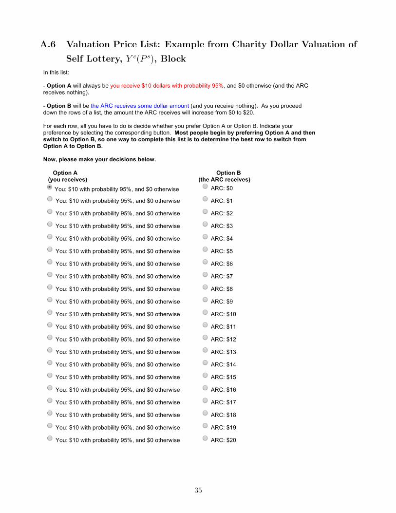
A.6 Valuation Price List: Example from Charity Dollar Valuation of

Self Lottery, Y c(P s), Block!Block 5 List 1

In this list: - Option A will always be you receive $10 dollars with probability 95%, and $0 otherwise (and the ARC receives nothing). - Option B will be the ARC receives some dollar amount (and you receive nothing). As you proceed down the rows of a list, the amount the ARC receives will increase from $0 to $20. For each row, all you have to do is decide whether you prefer Option A or Option B. Indicate your preference by selecting the corresponding button. Most people begin by preferring Option A and then switch to Option B, so one way to complete this list is to determine the best row to switch from Option A to Option B. Now, please make your decisions below. Option A (you receives)

Option B (the ARC receives)

You: $10 with probability 95%, and $0 otherwise ARC: $0

You: $10 with probability 95%, and $0 otherwise ARC: $1

You: $10 with probability 95%, and $0 otherwise ARC: $2

You: $10 with probability 95%, and $0 otherwise ARC: $3

You: $10 with probability 95%, and $0 otherwise ARC: $4

You: $10 with probability 95%, and $0 otherwise ARC: $5

You: $10 with probability 95%, and $0 otherwise ARC: $6

You: $10 with probability 95%, and $0 otherwise ARC: $7

You: $10 with probability 95%, and $0 otherwise ARC: $8

You: $10 with probability 95%, and $0 otherwise ARC: $9

You: $10 with probability 95%, and $0 otherwise ARC: $10

You: $10 with probability 95%, and $0 otherwise ARC: $11

You: $10 with probability 95%, and $0 otherwise ARC: $12

You: $10 with probability 95%, and $0 otherwise ARC: $13

You: $10 with probability 95%, and $0 otherwise ARC: $14

You: $10 with probability 95%, and $0 otherwise ARC: $15

You: $10 with probability 95%, and $0 otherwise ARC: $16

You: $10 with probability 95%, and $0 otherwise ARC: $17

You: $10 with probability 95%, and $0 otherwise ARC: $18

You: $10 with probability 95%, and $0 otherwise ARC: $19

You: $10 with probability 95%, and $0 otherwise ARC: $20

!

35

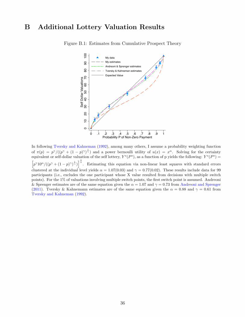
B Additional Lottery Valuation Results

Figure B.1: Estimates from Cumulative Prospect Theory

010

2030

4050

6070

8090

100

Self

Dol

lar V

alua

tions

0 .1 .2 .3 .4 .5 .6 .7 .8 .9 1Probability P of Non-Zero Payment

My dataMy estimatesAndreoni & Sprenger estimatesTversky & Kahneman estimatesExpected Value

In following Tversky and Kahneman (1992), among many others, I assume a probability weighting function

of π(p) = pγ/((pγ + (1 − p)γ)1γ ) and a power bernoulli utility of u(x) = xα. Solving for the certainty

equivalent or self-dollar valuation of the self lottery, Y s(P s), as a function of p yields the following: Y s(P s) =[pγ10α/((pγ + (1− p)γ)

1γ )] 1

α

. Estimating this equation via non-linear least squares with standard errors

clustered at the individual level yields α = 1.07(0.03) and γ = 0.77(0.02). These results include data for 99participants (i.e., excludes the one participant whose X value resulted from decisions with multiple switchpoints). For the 1% of valuations involving multiple switch points, the first switch point is assumed. Andreoni& Sprenger estimates are of the same equation given the α = 1.07 and γ = 0.73 from Andreoni and Sprenger(2011). Tversky & Kahnemann estimates are of the same equation given the α = 0.88 and γ = 0.61 fromTversky and Kahneman (1992).

36

Figure B.2: Decision Level Results

No Self-Charity Tradeoff

.3.4

.5.6

Frac

tion

of V

alua

tions

Charity Lottery Self Lottery

< Expected Value> Expected Value

Self-Charity Tradeoff

.3.4

.5.6

Frac

tion

of V

alua

tions

Charity Lottery Self Lottery

< Expected Value> Expected Value

The error bars show the confidence interval for two standard errors. The calculations for the no self-charitytradeoff context result from the charity-dollar valuations of charity lotteries, Y c(P c), and the self-dollarvaluations of self lotteries, Y s(P s). The calculations for the self-charity tradeoff context result from theself-dollar valuations of charity lotteries, Y s(P c), and the charity-dollar valuations of self lotteries, Y c(P s).Valuations in self-dollars are scaled as percentages of $10, and valuations in charity-dollars are scaled aspercentages of $Xi. The results include data for the 57 participants in my main subsample (i.e., excludesparticipants with X values that were censored or resulted from decisions with multiple switch points). Forthe 1% of valuations involving multiple switch points, the first switch point is assumed.

37

Table B.1: Lottery Valuations in No Self-Charity Tradeoff Context

Regression: Ordinary Least Squares Interval TobitDV: Yl Y lower

l , YlY upperl

1 2 3 4 5 6 7charity 0.06 0.06 0.24 -0.44 0.06 0.23 1.28

(0.82) (0.82) (0.87) (0.83) (0.83) (0.87) (0.80)

I(P = 0.95) 79.17∗∗∗

(1.71)

I(P = 0.90) 74.04∗∗∗

(1.80)

I(P = 0.75) 60.33∗∗∗

(1.69)

I(P = 0.50) 38.46∗∗∗

(1.49)

I(P = 0.25) 18.64∗∗∗

(1.02)

I(P = 0.10) 6.14∗∗∗

(0.85)

Constant 51.79∗∗∗ 51.79∗∗∗ 51.88∗∗∗ 51.85∗∗∗ 12.25∗∗∗ 51.83∗∗∗ 50.50∗∗∗

(0.96) (0.41) (0.44) (0.41) (1.43) (0.97) (0.80)Ind FE no yes yes yes no no noObs with MSP yes yes no no yes yes yesInd with MSP yes yes yes no yes yes yesCensored X no no no no no no yesObservations 798 798 792 700 798 798 1386Subjects 57 57 57 50 57 57 99

∗ p < 0.10, ∗∗ p < 0.05, ∗∗∗ p < 0.01. Standard errors are clustered at the individual leveland shown in parentheses. The dependent variables are lottery valuations Yl in the no self-charitytradeoff context - i.e., self-dollar valuations of self lotteries (Y s(P s)), and charity-dollar valuations ofcharity lotteries (Y c(P c)). Valuations in self-dollars are scaled as percentages of $10, and valuationsin charity-dollars are scaled as percentages of $Xi. The results are from regressions of Yli =β0 + β1charityli + (

∑P λP +

∑i µi) + εli, where Yli is the valuation of a lottery l by individual

i (in the case of the Tobit regression, this involves the upper and lower bounds of Yli); charity liis an indicator for charity lotteries; λP are fixed effects for lotteries with probability P ∈ {0.95,0.9, 0.75, 0.5, 0.25, 0.1} (P=0.05 excluded); µi are fixed effects for individual i (individual i = 1excluded). Probability fixed effects are shown when included, and “Ind FE” indicates whether or notindividual fixed effects are included. “Obs with MSP” and “Ind with MSP” indicate whether or notobservations with, or individuals that have observations with multiple switch points, respectively,are included. When observations involving multiple switch points are included, the first switchpoint is assumed. “Censored X” indicates whether or not participants with censored X values areincluded. Note that 1 participant is always excluded because their X value resulted from decisionswith multiple switch points.

38

Table B.2: (Self - Charity) Lottery Valuations in No Self-Charity Tradeoff Context

Regression: Ordinary Least Squares TobitDV: Dl Dl

1 2 3 4I(P = 0.95) -1.84∗ -1.84∗ -1.65∗ -2.58∗∗∗

(0.95) (0.95) (0.97) (0.86)

I(P = 0.90) -3.60∗∗∗ -3.60∗∗∗ -3.25∗∗ -3.21∗∗∗

(1.26) (1.26) (1.33) (1.02)

I(P = 0.75) -3.03∗∗ -3.03∗∗ -2.40∗ -4.75∗∗∗

(1.32) (1.32) (1.38) (1.23)

I(P = 0.50) 0.70 0.82 1.90 -0.61(1.73) (1.69) (1.57) (1.53)

I(P = 0.25) 2.11∗ 2.23∗ 2.50∗ 0.35(1.18) (1.20) (1.30) (1.22)

I(P = 0.10) 2.72 2.00 3.50∗∗ 1.97(1.86) (1.71) (1.57) (1.29)

I(P = 0.05) 2.54∗∗ 2.23∗∗ 2.50∗∗ 2.05∗∗

(1.12) (1.10) (1.19) (0.93)Ind FE no no no noObs with MSP yes no no yesInd with MSP yes yes no yesCensored X no no no yesObservations 399 393 350 693Subjects 57 57 50 99

∗ p < 0.10, ∗∗ p < 0.05, ∗∗∗ p < 0.01. Standard errors are clustered at the individual level and shownin parentheses. The dependent variables are differences in lottery valuations DP in the no self-charitytradeoff context - i.e., self-dollar valuations of self lotteries minus charity-dollar valuations of charity lotteries(Y s(P s) − Y c(P c)). Valuations in self-dollars are scaled as percentages of $10, and valuations in charity-dollars are scaled as percentages of $Xi. The results are from regressions of DPi =

∑P λP + εi, where

DPi is the difference in lottery valuations for probability P by individual i; λP are fixed effects for lotterieswith probability P ∈ {0.95, 0.9, 0.75, 0.5, 0.25, 0.1, 0.05}. Probability fixed effects are shown, and “IndFE” indicates whether or not individual fixed effects are included. “Obs with MSP” and “Ind with MSP”indicate whether or not observations with, or individuals that have observations with, multiple switch pointsare included. When observations involving multiple switch points are included, the first switch point isassumed. “Censored X” indicates whether or not participants with censored X values are included. Notethat 1 participant is always excluded because their X value resulted from decisions with multiple switchpoints.

39

Table B.3: Lottery Valuations in Self-Charity Tradeoff Context

Regression: Ordinary Least Squares Interval TobitDV: Yl Y lower

l , YlY upperl

1 2 3 4 5 6 7charity -15.04∗∗∗ -15.04∗∗∗ -15.49∗∗∗ -14.95∗∗∗ -15.04∗∗∗ -16.28∗∗∗ -46.64∗∗∗

(3.22) (3.22) (3.31) (3.61) (3.23) (3.56) (5.12)

I(P = 0.95) 61.60∗∗∗

(3.05)

I(P = 0.90) 58.60∗∗∗

(2.79)

I(P = 0.75) 49.01∗∗∗

(2.29)

I(P = 0.50) 34.41∗∗∗

(2.04)

I(P = 0.25) 17.63∗∗∗

(1.86)

I(P = 0.10) 5.88∗∗∗

(1.25)

Constant 57.09∗∗∗ 57.09∗∗∗ 57.51∗∗∗ 56.79∗∗∗ 24.65∗∗∗ 58.62∗∗∗ 78.52∗∗∗

(2.01) (1.61) (1.65) (1.81) (3.13) (2.32) (3.46)Ind FE no yes yes yes no no noObs with MSP yes yes no no yes yes yesInd with MSP yes yes yes no yes yes yesCensored X no no no no no no yesObservations 798 798 784 700 798 798 1386Subjects 57 57 57 50 57 57 99

∗ p < 0.10, ∗∗ p < 0.05, ∗∗∗ p < 0.01. Standard errors are clustered at the individual level and shown inparentheses. The dependent variables are lottery valuations Yl in the self-charity tradeoff context - i.e.,charity-dollar valuations of self lotteries (Y c(P s)), and self-dollar valuations of charity lotteries (Y s(P c)).Valuations in self-dollars are scaled as percentages of $10, and valuations in charity-dollars are scaled aspercentages of $Xi. The results are from regressions of Yli = β0 + β1charityli + (

∑P λP +

∑i µi) + εli,

where Yli is the valuation of a lottery l by individual i (in the case of the Tobit regression, this involvesthe upper and lower bounds of Yli); charity li is an indicator for charity lotteries; λP are fixed effectsfor lotteries with probability P ∈ {0.95, 0.9, 0.75, 0.5, 0.25, 0.1} (P=0.05 excluded); µi are fixed effectsfor individual i (individual i = 1 excluded). Probability fixed effects are shown when included, and“Ind FE” indicates whether or not individual fixed effects are included. “Obs with MSP” and “Ind withMSP” indicate whether or not observations with, or individuals that have observations with, multipleswitch points are included. When observations involving multiple switch points are included, the firstswitch point is assumed. “Censored X” indicates whether or not participants with censored X values areincluded. Note that 1 participant is always excluded because their X value resulted from decisions withmultiple switch points.

40

Table B.4: (Self - Charity) Lottery Valuations in Self-Charity Tradeoff Context

Regression: Ordinary Least Squares TobitDV: Dl Dl

1 2 3 4I(P = 0.95) 21.32∗∗∗ 20.97∗∗∗ 18.90∗∗∗ 43.71∗∗∗

(4.01) (4.18) (4.31) (3.93)

I(P = 0.90) 21.27∗∗∗ 20.76∗∗∗ 19.35∗∗∗ 44.08∗∗∗

(3.90) (3.94) (4.25) (3.90)

I(P = 0.75) 18.42∗∗∗ 18.75∗∗∗ 18.50∗∗∗ 42.88∗∗∗

(3.97) (4.03) (4.42) (4.01)

I(P = 0.50) 16.84∗∗∗ 17.27∗∗∗ 17.60∗∗∗ 40.05∗∗∗

(3.77) (3.89) (4.19) (4.14)

I(P = 0.25) 14.87∗∗∗ 15.50∗∗∗ 15.35∗∗∗ 38.18∗∗∗

(3.99) (4.07) (4.42) (4.33)

I(P = 0.10) 9.25∗∗∗ 10.51∗∗∗ 9.50∗∗∗ 33.79∗∗∗

(3.31) (3.41) (3.47) (4.33)

I(P = 0.05) 3.29 3.44 5.45∗ 28.59∗∗∗

(3.00) (3.05) (3.19) (4.34)Ind FE no no no noObs with MSP yes no no yesInd with MSP yes yes no yesCensored X no no no yesObservations 399 386 350 693Subjects 57 57 50 99

∗ p < 0.10, ∗∗ p < 0.05, ∗∗∗ p < 0.01. Standard errors are clustered at the individual level and shownin parentheses. The dependent variables are differences in lottery valuations Dp in the self-charity trade-off context - i.e., charity-dollar valuations of self lotteries minus self-dollar valuations of charity lotteries(Y c(P s) − Y s(P c)). Valuations in self-dollars are scaled as percentages of $10, and valuations in charity-dollars are scaled as percentages of $Xi. The results are from regressions of DPi =

∑P λP + εi, where

DPi is the difference in lottery valuations for probability P by individual i; λP are fixed effects for lotterieswith probability P ∈ {0.95, 0.9, 0.75, 0.5, 0.25, 0.1, 0.05}. Probability fixed effects are shown, and “IndFE” indicates whether or not individual fixed effects are included. “Obs with MSP” and “Ind with MSP”indicate whether or not observations with, or individuals that have observations with, multiple switch pointsare included. When observations involving multiple switch points are included, the first switch point isassumed. “Censored X” indicates whether or not participants with censored X values are included. Notethat 1 participant is always excluded because their X value resulted from decisions with multiple switchpoints.

41

Table B.5: Charity Lottery Valuations

Regression: Ordinary Least Squares Interval TobitDV: Yl Y lower

l , Y upperl Yl

1 2 3 4 5 6 7tradeoff -9.79∗∗∗ -9.79∗∗∗ -9.98∗∗∗ -9.57∗∗∗ -9.79∗∗∗ -9.72∗∗∗ -19.91∗∗∗

(1.89) (1.89) (1.94) (2.13) (1.90) (1.95) (2.00)

I(P = 0.95) 66.97∗∗∗

(2.42)

I(P = 0.90) 63.36∗∗∗

(2.19)

I(P = 0.75) 52.28∗∗∗

(1.85)

I(P = 0.50) 33.51∗∗∗

(1.41)

I(P = 0.25) 15.35∗∗∗

(1.19)

I(P = 0.10) 4.47∗∗∗

(0.67)

Constant 51.85∗∗∗ 51.85∗∗∗ 52.13∗∗∗ 51.41∗∗∗ 18.14∗∗∗ 52.05∗∗∗ 51.75∗∗∗

(0.83) (0.94) (0.96) (1.06) (1.66) (0.87) (0.80)Ind FE no yes yes yes no no noObs with MSP yes yes no no yes yes yesInd with MSP yes yes yes no yes yes yesCensored X no no no no no no yesObservations 798 798 788 700 798 798 1386Subjects 57 57 57 50 57 57 99

∗ p < 0.10, ∗∗ p < 0.05, ∗∗∗ p < 0.01. Standard errors are clustered at the individual level and shownin parentheses. The dependent variables are charity lottery valuations Yl - i.e., charity-dollar valuationsof charity lotteries (Y c(P c)), and self-dollar valuations of charity lotteries (Y s(P c)). Valuations in self-dollars are scaled as percentages of $10, and valuations in charity-dollars are scaled as percentages of$Xi. The results are from regressions of Yli = β0 + β1tradeoffli + (

∑P λP +

∑i µi) + εli, where Yli is the

valuation of a lottery l by individual i (in the case of the Tobit regression, this involves the upper andlower bounds of Yli); tradeoff li is an indicator for valuations occurring in the self-charity tradeoff context ;λP are fixed effects for lotteries with probability P ∈ {0.95, 0.9, 0.75, 0.5, 0.25, 0.1} (P=0.05 excluded);µi are fixed effects for individual i (individual i = 1 excluded). Probability fixed effects are shown, and“Ind FE” indicates whether or not individual fixed effects are included. “Obs with MSP” and “Ind withMSP” indicate whether or not observations with, or individuals that have observations with, multipleswitch points are included. When observations involving multiple switch points are included, the firstswitch point is assumed. “Censored X” indicates whether or not participants with censored X values areincluded. Note that 1 participant is always excluded because their X value resulted from decisions withmultiple switch points.

42

Table B.6: Self Lottery Valuations

Regression: Ordinary Least Squares Interval TobitDV: Yl Y lower

l , Y upperl Yl

1 2 3 4 5 6 7tradeoff 5.30∗∗ 5.30∗∗ 5.56∗∗∗ 4.94∗∗ 5.30∗∗ 6.90∗∗∗ 28.68∗∗∗

(2.02) (2.02) (2.03) (2.21) (2.02) (2.34) (3.85)

I(P = 0.95) 73.79∗∗∗

(1.87)

I(P = 0.90) 69.28∗∗∗

(1.86)

I(P = 0.75) 57.06∗∗∗

(1.71)

I(P = 0.50) 39.36∗∗∗

(1.68)

I(P = 0.25) 20.92∗∗∗

(1.47)

I(P = 0.10) 7.54∗∗∗

(1.09)

Constant 51.79∗∗∗ 51.79∗∗∗ 51.84∗∗∗ 51.85∗∗∗ 13.51∗∗∗ 51.83∗∗∗ 50.51∗∗∗

(0.96) (1.01) (1.01) (1.11) (1.39) (0.97) (0.80)lnsigmaConstant 3.50∗∗∗

(0.02)Ind FE no yes yes yes no no noObs with MSP yes yes no no yes yes yesInd with MSP yes yes yes no yes yes yesCensored X no no no no no no yesObservations 798 798 788 700 798 798 1386Subjects 57 57 57 50 57 57 99

∗ p < 0.10, ∗∗ p < 0.05, ∗∗∗ p < 0.01. Standard errors are clustered at the individual level and shownin parentheses. The dependent variables are self lottery valuations Yl - i.e., self-dollar valuations of selflotteries (Y s(P s)), and charity-dollar valuations of self lotteries (Y c(P s)). Valuations in self-dollars arescaled as percentages of $10, and valuations in charity-dollars are scaled as percentages of $Xi. Theresults are from regressions of Yli = β0 + β1tradeoffli + (

∑P λP +

∑i µi) + εli, where Yli is the valuation

of a lottery l by individual i (in the case of the Tobit regression, this involves the upper and lower boundsof Yli); tradeoff li is an indicator for valuations occurring in the self-charity tradeoff context ; λP are fixedeffects for lotteries with probability P ∈ {0.95, 0.9, 0.75, 0.5, 0.25, 0.1} (P=0.05 excluded); µi are fixedeffects for individual i (individual i = 1 excluded). Probability fixed effects are shown, and “Ind FE”indicates whether or not individual fixed effects are included. “Obs with MSP” and “Ind with MSP”indicate whether or not observations with, or individuals that have observations with, multiple switchpoints are included. When observations involving multiple switch points are included, the first switchpoint is assumed. “Censored X” indicates whether or not participants with censored X values are included.Note that 1 participant is always excluded because their X value resulted from decisions with multipleswitch points.

43

Table B.7: Lottery Valuations in Self Dollar Valuations

Regression: Ordinary Least Squares Interval TobitDV: Yl Y lower

l , Y upperl Yl

1 2 3 4 5 6 7tradeoff -9.74∗∗∗ -9.74∗∗∗ -9.90∗∗∗ -10.01∗∗∗ -9.74∗∗∗ -9.51∗∗∗ -18.67∗∗∗

(1.79) (1.79) (1.83) (1.98) (1.79) (1.84) (1.79)

I(P = 0.95) 64.78∗∗∗

(2.47)

I(P = 0.90) 60.29∗∗∗

(2.40)

I(P = 0.75) 49.50∗∗∗

(2.10)

I(P = 0.50) 32.59∗∗∗

(1.53)

I(P = 0.25) 15.13∗∗∗

(1.28)

I(P = 0.10) 4.56∗∗∗

(0.72)

Constant 51.79∗∗∗ 51.79∗∗∗ 51.97∗∗∗ 51.85∗∗∗ 19.39∗∗∗ 51.82∗∗∗ 50.49∗∗∗

(0.96) (0.89) (0.91) (0.99) (1.62) (0.97) (0.79)Ind FE no yes yes yes no no noObs with MSP yes yes no no yes yes yesInd with MSP yes yes yes no yes yes yesCensored X no no no no no no yesObservations 798 798 788 700 798 798 1386Subjects 57 57 57 50 57 57 99

∗ p < 0.10, ∗∗ p < 0.05, ∗∗∗ p < 0.01. Standard errors are clustered at the individual level and shownin parentheses. The dependent variables are lottery valuations elicited in self-dollar valuations Yl - i.e.,self-dollar valuations of self lotteries (Y s(P s)), and self-dollar valuations of charity lotteries (Y s(P c)).Valuations in self-dollars are scaled as percentages of $10. The results are from regressions of Yli = β0 +β1charityli + (

∑P λP +

∑i µi) + εli, where Yli is the valuation of a lottery l by individual i (in the case

of the Tobit regression, this involves the upper and lower bounds of Yli); tradeoff li is an indicator forvaluations occurring in the self-charity tradeoff context ; λP are fixed effects for lotteries with probability P∈ {0.95, 0.9, 0.75, 0.5, 0.25, 0.1} (P=0.05 excluded); µi are fixed effects for individual i (individual i = 1excluded). Probability fixed effects are shown, and “Ind FE” indicates whether or not individual fixedeffects are included. “Obs with MSP” and “Ind with MSP” indicate whether or not observations with, orindividuals that have observations with, multiple switch points are included. When observations involvingmultiple switch points are included, the first switch point is assumed. “Censored X” indicates whether ornot participants with censored X values are included. Note that 1 participant is always excluded becausetheir X value resulted from decisions with multiple switch points.

44

Table B.8: Lottery Valuations in Charity Dollar Valuations

Regression: Ordinary Least Squares Interval TobitDV: Yl Y lower

l , Y upperl Yl

1 2 3 4 5 6 7tradeoff 5.24∗∗ 5.24∗∗ 5.41∗∗∗ 5.38∗∗ 5.24∗∗ 6.73∗∗∗ 27.77∗∗∗

(1.97) (1.97) (1.98) (2.18) (1.98) (2.28) (3.75)

I(P = 0.95) 75.99∗∗∗

(1.74)

I(P = 0.90) 72.35∗∗∗

(1.57)

I(P = 0.75) 59.85∗∗∗

(1.33)

I(P = 0.50) 40.29∗∗∗

(1.24)

I(P = 0.25) 21.14∗∗∗

(1.40)

I(P = 0.10) 7.46∗∗∗

(1.12)

Constant 51.85∗∗∗ 51.85∗∗∗ 52.04∗∗∗ 51.41∗∗∗ 12.27∗∗∗ 52.08∗∗∗ 51.89∗∗∗

(0.83) (0.99) (0.99) (1.09) (1.29) (0.88) (0.82)Ind FE no yes yes yes no no noObs with MSP yes yes no no yes yes yesInd with MSP yes yes yes no yes yes yesCensored X no no no no no no yesObservations 798 798 788 700 798 798 1386Subjects 57 57 57 50 57 57 99

∗ p < 0.10, ∗∗ p < 0.05, ∗∗∗ p < 0.01. Standard errors are clustered at the individual level and shownin parentheses. The dependent variables are lottery valuations elicited in charity-dollar valuations Yl -i.e., charity-dollar valuations of charity lotteries (Y c(P c)), and charity-dollar valuations of self lotteries(Y c(P s)). Valuations in charity-dollars are scaled as percentages of $Xi. The results are from regressionsof Yli = β0 + β1tradeoffli + (

∑P λP +

∑i µi) + εli, where Yli is the valuation of a lottery l by individual

i (in the case of the Tobit regression, this involves the upper and lower bounds of Yli); tradeoff li is anindicator for valuations occurring in the self-charity tradeoff context ; λP are fixed effects for lotteries withprobability P ∈ {0.95, 0.9, 0.75, 0.5, 0.25, 0.1} (P=0.05 excluded); µi are fixed effects for individuali (individual i = 1 excluded). Probability fixed effects are shown, and “Ind FE” indicates whether ornot individual fixed effects are included. “Obs with MSP” and “Ind with MSP” indicate whether or notobservations with, or individuals that have observations with, multiple switch points are included. Whenobservations involving multiple switch points are included, the first switch point is assumed. “CensoredX” indicates whether or not participants with censored X values are included. Note that 1 participant isalways excluded because their X value resulted from decisions with multiple switch points.

45

Table B.9: Examining Ordering Effects

Regression: Ordinary Least SquaresDV: Yl

Charity Lotteries First Valued in Self Lotteries First Valued inSelf-Charity Tradeoff Context: Self-Charity Tradeoff Context:

Yes No Yes Nocharity 1.01 -1.25 -0.17 0.30

(1.21) (1.00) (0.99) (1.36)

tradeoff 5.38∗ 5.19∗ 4.61 6.07∗∗

(2.86) (2.81) (3.16) (2.48)

charity*tradeoff -16.88∗∗∗ -12.63∗∗ -14.43∗∗ -15.83∗∗∗

(4.53) (5.22) (5.44) (4.00)

Constant 50.73∗∗∗ 53.26∗∗∗ 51.80∗∗∗ 51.79∗∗∗

(0.97) (0.61) (0.90) (0.84)Ind FE yes yes yes yesObs with MSP yes yes yes yesInd with MSP yes yes yes yesCensored X no no no noObservations 924 672 840 756Subjects 33 24 30 27

∗ p < 0.10, ∗∗ p < 0.05, ∗∗∗ p < 0.01. Standard errors are clustered at the individual level and shown inparentheses. The dependent variables are lottery valuations Yl - i.e., self-dollar valuations of self lotteries(Y s(P s)), charity-dollar valuations of charity lotteries (Y c(P c)), charity-dollar valuations of self lotteries(Y c(P s)), and self-dollar valuations of charity lotteries (Y s(P c)). Valuations in self-dollars are scaled aspercentages of $10, and valuations in charity-dollars are scaled as percentages of $Xi. The results arefrom regressions of Equation 2. “Ind FE” indicates whether or not individual fixed effects are included.“Obs with MSP” and “Ind with MSP” indicate whether or not observations with, or individuals that haveobservations with, multiple switch points are included. When observations involving multiple switch pointsare included, the first switch point is assumed. “Censored X” indicates whether or not participants withcensored X values are included. Note that 1 participant is always excluded because their X value resultedfrom decisions with multiple switch points.

46

Table B.10: Lottery Valuations in Partner Study

Regression: Ordinary Least Squares Interval TobitDV: Yl Y lower

l , Y upperl Yl

1 2 3 4 5 6 7charity 1.90 1.90 1.90 1.67 1.90 1.90 -0.02

(1.24) (1.24) (1.24) (1.29) (1.24) (1.24) (1.53)

tradeoff 10.17∗∗∗ 10.17∗∗∗ 10.37∗∗∗ 11.59∗∗∗ 10.17∗∗∗ 12.07∗∗∗ 20.20∗∗∗

(3.41) (3.41) (3.39) (3.51) (3.42) (3.88) (3.99)

charity*tradeoff -22.54∗∗∗ -22.54∗∗∗ -22.61∗∗∗ -23.65∗∗∗ -22.54∗∗∗ -24.32∗∗∗ -35.60∗∗∗

(5.25) (5.25) (5.28) (5.57) (5.27) (5.72) (5.40)

I(P = 0.95) 65.80∗∗∗

(2.25)

I(P = 0.90) 61.51∗∗∗

(2.29)

I(P = 0.75) 50.28∗∗∗

(2.16)

I(P = 0.50) 35.24∗∗∗

(1.59)

I(P = 0.25) 17.07∗∗∗

(1.20)

I(P = 0.10) 5.95∗∗∗

(0.65)

Constant 49.69∗∗∗ 49.69∗∗∗ 49.72∗∗∗ 50.17∗∗∗ 16.00∗∗∗ 49.69∗∗∗ 49.64∗∗∗

(1.42) (0.84) (0.83) (0.86) (1.79) (1.42) (1.10)Ind FE no yes yes yes no no noObs with MSP yes yes no no yes yes yesInd with MSP yes yes yes no yes yes yesCensored X no no no no no no yesObservations 812 812 810 756 812 812 1176Subjects 29 29 29 27 29 29 42

∗ p < 0.10, ∗∗ p < 0.05, ∗∗∗ p < 0.01. Standard errors are clustered at the individual level and shown in parentheses.The dependent variables are lottery valuations Yl - i.e., self-dollar valuations of self lotteries (Y s(P s)), partner-dollar valuations of partner lotteries (Y p(P p)), partner-dollar valuations of self lotteries (Y p(P s)), and self-dollarvaluations of partner lotteries (Y s(P p)). Valuations in self-dollars are scaled as percentages of $10, and valuationsin charity-dollars are scaled as percentages of $X. The results are from regressions of Equation 2 modified suchthat charity is replaced by partner. Probability fixed effects are shown when included, and “Ind FE” indicateswhether or not individual fixed effects are included. “Obs with MSP” and “Ind with MSP” indicate whetheror not observations with, or individuals that have observations with, multiple switch points are included. Whenobservations involving multiple switch points are included, the first switch point is assumed. “Censored X”indicates whether or not participants with censored X values are included. Note that 2 participants are alwaysexcluded because their X values resulted from decisions with multiple switch points.

47

C Additional Moral Wiggle Room Task Results

Table C.1 shows the percentages of participants choosing A across the three questions. First,

consider the cases where the state is always revealed - i.e., in the revealed-aligned-state question

or revealed-unaligned-state question. When payoffs are aligned, 100% of participants choose the

dominant optionA, or their choices implyA : ($6, $5) � B : ($5, $1). When payoffs are unaligned,

only 44% choose the now selfish option A, or their choices imply A : ($6, $1) � B : ($5, $5). This

shows that most participants are willing to sacrifice some of their own payoffs in return for higher

charity payoffs.

To begin considering if participants are more likely to choose the selfish option in the choice-to-

reveal question, let us first abstract away from whether or not participants reveal their state.32

For participants in the aligned state, their choices are nearly identical to their choices in the

revealed-aligned-state question: 97.96% choose A. However, for participants in the unaligned

state, their choices become substantially more selfish compared to their choices in the revealed-

unaligned-state question: 68.63% choose A. As shown in the third row of Table C.1, 68.63% of

the participants choosing the selfish option is significantly larger than the 39.22% of the same

participants who choose the selfish option in the revealed-unaligned-state question (a t-test rejects

the equality of these percentages with p < 0.0001).

Table C.1: Percentage of Participants Choosing A According to Their State and Question Asked

Revealed-State Choice-to-RevealQuestions Question

For participants in:Aligned State 100.00% 97.96%A : ($6, $5), B : ($5, $1) (n=100) (n=49)

Unaligned State 44.00% 68.63%A : ($6, $1), B : ($5, $5) (n=100) (n=51)

Unaligned State* 39.22% 68.63%A : ($6, $1), B : ($5, $5) (n=51) (n=51)

The bundle (U, V ) corresponds with the participant receiving $U andthe charity receiving $V. n denotes the relevant sample size for each cell.In the third row, * indicates that the sample is restricted to participantswho had the aligned state payments of A : ($6, $1) and B : ($5, $5) inthe choice-to-reveal question.

As shown in Table C.2, the increased selfish behavior in the choice-to-reveal question seems

to result from participants avoiding information about whether or not their choice of A is selfish.

32For participants who choose to reveal their state, the survey software, Qualtrics, randomly assigns them toone of the two states. For participants who do not choose to reveal their state, I replicate what Qualtrics wouldhave done by randomly assigning them to one of the two states.

48

For participants in the unaligned state, 54.90% choose to not reveal their state, and among these

participants, 100% choose the selfish option A. Similarly, for participants in the aligned state,

55.10% chose not to reveal their state, and among these participants, 96.30% choose A. While

choosing A is not selfish in the aligned state, it provides the same evidence for excuse-driven

behavior; from the perspective of the participants, they choose A which maximizes their payoffs

while avoiding information on whether or not A also maximizes the charity’s payoffs.

Table C.2: Percentage of Participants Choosing A in Choice-to-Reveal Question

Among participants whoChoose No Reveal Choose Reveal

Aligned State 96.30% 100.00%A : ($6, $5), B : ($5, $1) (n=27) (n=22)

Unaligned State 100.00% 30.43%A : ($6, $1), B : ($5, $5) (n=28) (n=23)

The bundle (U, V ) corresponds with the participant receiving $U andthe charity receiving $V. n denotes the relevant sample size for each cell.This data is only from the choice-to-reveal question, where participantscould choose to reveal their state or choose not to reveal their state,before choosing A or B.

49