excitation of the primary tropospheric chemical mode in...

JOURNAL OF GEOPHYSICAL RESEARCH, VOL. 105, NO. D20, PAGES 24,647-24,660, OCTOBER 27, 2000

Excitation of the primary tropospheric chemical mode in a global three-dimensional model

Oliver Wild Michael J. Prather

Earth System Science, University of California, Irvine

Abstract. Coupling of local chemical processes over the globe by atmospheric transport leads to the existence of chemical modes that are a fundamental characterization of global atmospheric chemistry and provide a true description of the atmospheric response to small changes in trace-gas emissions. Such coupled chemistry-transport modes in global tropospheric chemistry are an inherent feature of three-dimensional chemical transport models (CTMs). In CTMs these modes cannot be solved for explicitly, as they have been for the case of low-order, fully linearized systems, but they are investigated here through a series of perturbation experiments. When using meteorological fields that recycle every year, the long-lived modes are readily seen as seasonal decay patterns that e-fold each year. An important application of chemical modes is the study of how emissions of CO and NO excite perturbations to the CH4-1ike mode, the longest-lived (primary) mode found in tropospheric chemistry (i.e., with fixed stratospheric composition). Perturbation experiments are conducted with the University of California, Irvine, three-dimensional tropospheric CTM to identify this primary tropospheric mode and to determine its five-dimensional structure. The previous demonstrations of a long-lived chemical mode with 1.5 times the lifetime of CH4 are corroborated. The ability of emissions of CO and NO to excite this mode is then demonstrated, and a quantitative evaluation of the indirect effect of CO emissions on the greenhouse gases CH4 and tropospheric O• is made, showing that 100 kg of CO is equivalent to 5-6 kg of CH4 emissions.

1. Introduction

The chemical composition of the atmosphere is controlled by many natural processes that add, remove, and transform the key constituents. Trace gases may be introduced by direct emissions or by chemical formation processes, may be transported short distances or around the globe, and may be removed by insitu chemical trans- formations or by deposition to the surface. Spatial and temporal variations are natural features of chemical species in the global atmosphere. Coupling between photochemical and transport processes leads to the existence of global, chemical modes (i.e., specific spatial and temporal variations) that are fundamental characteris- tics of the atmospheric system [Prather, 1994]. These natural chemical modes are defined as general solutions to the linearized continuity equations, and they are re-

X Now at the Frontier Research System for Global Change, Yokohama, Japan.

Copyright 2000 by the American Geophysical Union.

Paper number 2000JD900399. 0148-0227 / 00 / 2000 JD900399509.00

vealed in the atmosphere as five-dimensional patterns, varying with three spatial dimensions, time, and chemical species. Each mode describes a particular combination of chemistry and transport and gives rise to a specific pattern of variation in species concentrations, with amplitudes and distribution controlled by the coupling involved. Each has a characteristic timescale (an e-folding decay time) defined by the respective eigen- value. The ensemble of modes defines the entire system, although the number of modes in a global, 3-D annual cycle of tropospheric chemistry is too large to compute. The theory of modes is detailed by Prather [1996], and additional box-model examples of the CH4- CO-OH system are given by Daniel and Solomon [1998] and Manning [1999].

Knowledge of these natural modes can help in predic- tion of the atmosphere's response to changing anthropogenic emissions. Most human perturbations to the chemical composition of the atmosphere over the past several decades may be described by excitation of a linear combination of the chemical modes, each of which decays with its characteristic e-folding time. The lifetime of the longest-lived, excited mode provides a bet- ter measure of the duration of the chemical perturbation than the steady state lifetimes of individual compo-

24,647

24,648 WILD AND PRATHER: TROPOSPHERIC CHEMICAL MODES IN 3-D MODELS

nents of the system [Prather, 1994]. In simple systems with few components and a limited number of degrees of freedom, the modes can be solved for analytically, as demonstrated for box models of the CH4-CO-OH system. This paper extends these studies to the global, three-dimensional, tropospheric chemistry system, determining the primary, decadal-scale mode through numerical perturbation experiments. The stratosphere is fixed, and thus century-scale perturbations (associated primarily with N20) do not arise. Using the Universi- ty of California, Irvine (UCI), chemical transport model (CTM), we map the seasonal and spatial variation of the many chemical species that are part of this mode and calculate an e-folding time of 14.2 years compared with the global atmospheric lifetime for CH4 of 9.7 years. Additional numerical experiments show how this mode is excited by the short-lived species NO and CO, re- vealing those parts of the atmosphere that are most or least sensitive to emissions in terms of global chemical perturbations.

In section 2 we describe the UCI tropospheric CT- M used in these studies and briefly evaluate its perfor- mance in simulating the chemistry of the current troposphere by comparing it with recent measurements. In section 3 we identify the primary mode present in this tropospheric chemical system and characterize both s- patial and seasonal variations of the key atmospheric species. We show how this mode may be excited by emissions of CH4, CO, and NOx in section 4 and then quantify the indirect climate forcing that the seeming- ly short lived, radiatively inactive gas CO may have through its excitation of the greenhouse gases CH4 and tropospheric O3 in the long-lived, primary mode. A summary and future directions for chemical mode studies are given in section 5.

2. The U CI CTM

2.1. Model Description

The UCI CTM is the latest in a generation of models developed at UCI based on meteorological fields from the Goddard Institute of Space Sciences (GISS) general circulation model (GCM). Previous versions of the model have been used to study the dynamics of the troposphere [Prather et al., 1987], the distributions and correlations of stratospheric trace gases [Hall and Prather, 1995; Avallone and Prather, 1997], and the impact of cometary water on the stratosphere [Hannegan et al., 1998]. The model uses meteorological fields from the new GISS II • GCM that have been tested for tracer

transport in both troposphere [Rind and Lerner, 1996; Koch and Rind, 1998] and stratosphere [Hall et al., 1999]. The tropospheric version at UCI uses 3-hour averaged fields with a horizontal resolution of 4 ø latitude x 5 ø longitude, and a vertical resolution of nine levels from the surface to 10 hPa, with six to eight levels in the troposphere. Advection is calculated using

the Prather scheme conserving second-order moments [Prather, 1986]. Entraining and nonentraining convective mass fluxes are supplied as 3-hour averages from the meteorological fields. The height of the boundary layer is diagnosed from the fields, and a bulk-mixing scheme is applied, mixing the full depth of the layer every CTM time step.

A detailed tropospheric chemical scheme has been included in the model using the ASAD modular chemistry package [Carver et al., 1997], with a fast implicit solver for the chemical equations. The scheme includes an ex- plicit treatment of inorganic HOx/Ox/NOx chemistry and methane oxidation and a lumped "family" treatment of hydrocarbon oxidation for the representative species butane, propene, xylene, and isoprene. A total of 32 species are considered, with 25 species transported and seven reinitialized to local steady state at each time step. Reaction rates are based on the recommendation- s of DeMote et al. [1997] and Atkinson et al. [1997], with additional rates from Hough [1991] and from the Leeds University Master Chemical Mechanism (MCM) [Jenkin et al., 1997].

Photolysis rates are calculated using the Fast-J photolysis scheme [Wild et al., 2000], which has an on-line treatment of molecular and aerosol absorption and scat- tering. Ozone, temperature, surface albedo, and cloud optical depth are supplied from the CTM or meteorological fields every 3 hours; the optical depth is appor- tioned between different water droplet sizes and phas-

Table 1. Global Annual Emission Rates of Trace Gases

Used in the University of California, Irvine, Chemical Transport Model

Trace Gas Source Resolution Annual Flux

NO•,, Tg N yr -1 industrial a 1 ø x 1 ø 20.97 soil b 1 ø x 1 ø 5.48 bioburn c 4 ø x 5 ø 11.64

lightning d 5.00 aircraft e 1 ø x 1 ø 0.51

CO, Tg yr -1 industrial c 4 ø x 5 ø 390.90 wood fuel c 4 ø x 5 ø 128.80 bioburn c 4 ø x 5 ø 517.40 ocean f 1 ø x 1 ø 13.00

CH4, Tg yr -• all sources g 1 ø x 1 ø 490.00 NMHC, Tg yr -1 industrial h 1 ø x 1 ø 109.37

isoprene i 1 ø x 1 ø 569.00

a Benkovitz et al. [1996]. b Yienger and Levy [1995]. ½ Wang et al. [1998]; J. Logan (personal communication,

1997). dBased on Price and Rind [1992]. e Baughcum et al. [1996]. f Bates et al. [1995]. g Fung et al. [1991]. hpiccot et al. [1992]. i Guenther et al. [1995].

WILD AND PRATHER: TROPOSPHERIC CHEMICAL MODES IN 3-D MODELS 24,649

es depending on the cloud type. This allows the full variability of photolysis rates to be captured on short timescales, as cloud and aerosol fields vary. Fast-J is a significant step forward coupling ozone, aerosols, and clouds in global CTMs, although it still does not ad- dress the problems of partial cloud cover in a grid cell.

Emissions of trace species are taken from the Global Emissions Inventory Activity inventories at 1 ø x 1 ø resolution, (see Table 1), and mapped onto the CTM grid. Information on gradients within the model grid cells is provided as moments in the lowest CTM level. Addi- tional emissions for CO and biomass burning sources at 4 ø x 5 ø resolution are from Wang et al. [1998] (J. Lo- gan, personal communication, 1997). Diurnal variations are provided for industrial and biogenic sources; seasonal variations are provided for soil emissions, methane, and biomass burning sources. A source of NO from lightning, 5 Tg N yr -1, is included based on the parameterization of Price and Rind [1992] but using the vertical mass flux from the meteorological fields to define deep convective events and to distribute the source proportionally. A source of NO from aircraft, 0.5 Tg N yr -1, at 1 ø x 1 ø by 1-km resolution is included from the NASA 1992 emissions data set for subsonic aircraft

[Baughcum et al., 1996]. Dry deposition is treated by using 1-m deposition ve-

locities based on Hough [1991] and vegetation type taken from the 1 ø x 1 ø vegetation and cultivation data sets of Mathews [1983]; correction of deposition velocities to the center of the lowest model level is based on the K-

theory of Isaksen et al. [1985]. Wet deposition, through removal of a fraction of soluble species from wet convective updrafts, is based on Balkanski et al. [1993]. Washout, or below-cloud scavenging, is treated with a simple first-order removal lifetime [Logan et al., 1981], increasing with altitude and reflecting the solubility of the species.

Calculation of the tropospheric chemical tendencies under stratospheric conditions is unnecessary here and can produce so,ne undesired numerical artifacts, es- pecially in stratosphere-troposphere exchange fluxes. Thus the U CI CTM carries a synthetic O3-1ike tracer which is used to distinguish instantaneously between stratospheric and tropospheric "air" for each 3-D grid cell. This approach allows for separate chemical treat- ments and works particularly well in the case of tropopause folds for which no clear tropopause height can be defined. The additional tracer, "Synoz", is forced with a stratospheric source in the uppermost CTM level and is removed in the lowest 2 km of the model by resetting it to 30 ppbv. This technique is described in detail by McLinden et al. [2000]. The 120-ppbv isopleth of the annually repeating distribution of the tracer is used to define the tropopause. Below this isopleth, tropospheric chemistry is applied; above, the effects of stratospheric chemistry are simulated by imposing a first-order decay on many species to ensure that they are not returned

to the troposphere. A source of ozone is supplied in the highest layer, 475 Tg yr -1 (as for Synoz), based on our assessment of tracer correlations in the midlati-

tude stratosphere [Murphy and Fahey, 1994; McLinden et al., 2000], and a source for the NO v species, 0.45 Tg N yr -1, is likewise injected with an HONO2:NOx ratio of 4:1. Since there is no chemistry applied when the $ynoz tracer exceeds 120 ppbv, this technique ensures control of the global, annual mean net stratospheric influx of NOx, HONO2, and 03.

This numerical study of tropospheric chemical modes requires some computationally necessary compromises along with strict control of the degrees of freedom. With multiyear integrations required, we chose to increase the grid size of the CTM to 8 ø x 10 ø by combining variables at 4 ø x 5 ø, a large saving in computational time without significant loss of accuracy. The single year of GCM meteorological fields has been repeated for multiyear runs, thus providing a clear e-folding of the primary mod- e and avoiding the noise caused by interannual variability. A fixed, parameterized stratospheric chemistry is used to ensure that the primary mode reflects only the chemistry of the troposphere; with full stratospheric chemistry the primary mode would be dominated by N20, which has a century-long timescale, much greater than any of the species important in tropospheric chemistry [Prather, 1998]. This mode study requires that all tropospheric species be driven with flux boundary conditions, as use of fixed mixing ratio conditions would prevent derivation of the correct modes.

2.2. Model Evaluation

A brief characterization of the model is made by comparing the simulation for circa 1990 conditions against surface and profile measurements. The GISS IF fields used here represent a typical meteorological year rather than a specific year, and therefore this evaluation focus- es on observational monthly statistics, where available. The physical schemes used to derive the meteorology in the GISS II • GCM have been assessed by Rind and Lerner [1996]. While the main features of the tropospheric circulation are well reproduced, the model tends to overpredict the degree of tropospheric-stratospheric exchange due to the rather oversimplified stratospheric circulation when considering only nine vertical lay- ers [Rind et al., 1999]. The cloud coverage is consistent with the International Satellite Cloud Climatology Project (ISCCP) cloud climatology, and the mean optical depths, used by the photolysis scheme, are similar. In the following chemical evaluation the concentrations of long-lived species are initialized in the CTM with zonal mean concentrations taken from the Cambridge 2-D model [Law and Pyle, 1993], and results are pre- sented from the third year of the model simulation, by which time the initialization, except for the mean CH4 concentration, has little influence.


60

40

20

0

60

•> 40 o

• 20

= 60

•o 40 o

2O

0

6O

4O

2O

0

Point Barrow, 70N

I I I I I I I I l I I I

Mauna Loa, 20N

Natal, 6S

Cape Grim 41S

1 2 3 4 5 6 7 8 9 101112

Month

60

40

20

0

60

40

20

0

60

40

20

0

60

40

20

0

ß ß ß ß ß ß H:ohe•npe•isse•nb•erg,,48•N • , , Barbados, 13N

I I I I I I I I i I I

Samoa, 14S

ß ß ß ß .. ., ß ß I I I I I I I I i I I

South Pole, 90S

1 2 3 4 5 6 7 8 9 101112

Month

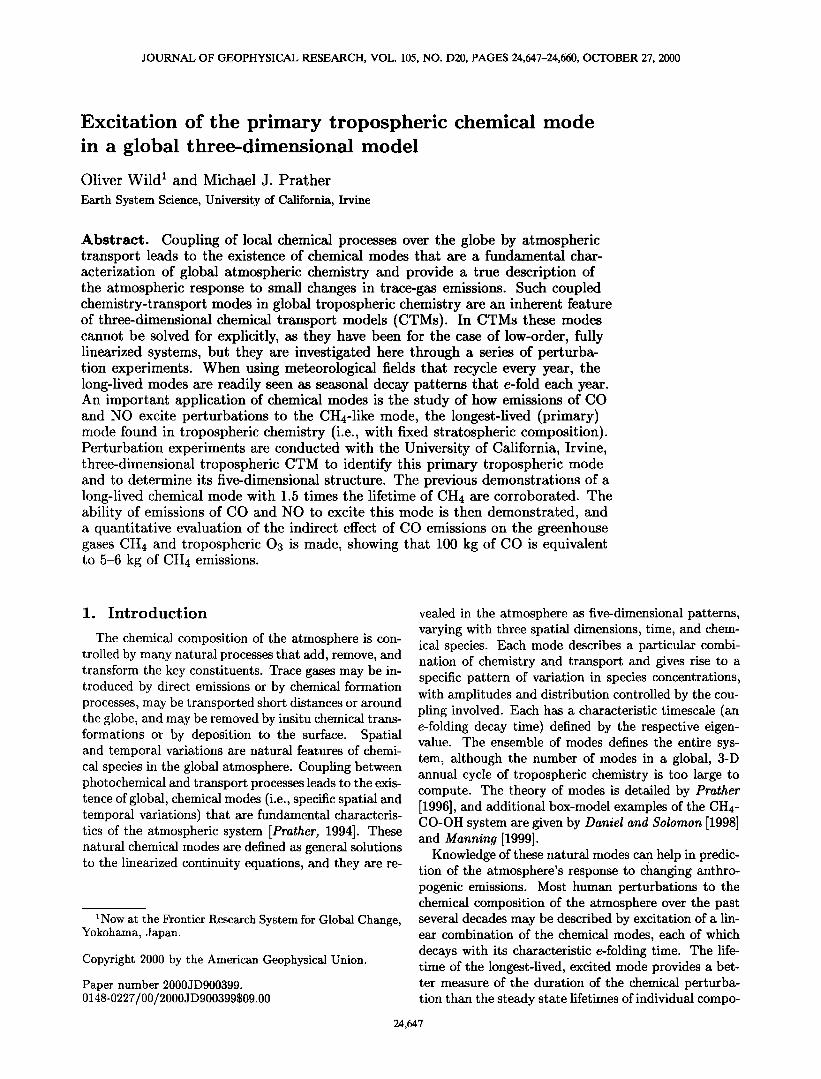
Figure 1. Monthly-mean modeled (solid lines) and observed (dots) mixing ratios of 03 at surface measurement sites. All observational data are from Oltmans and Levy [1994], with the exception of Hohenpeissenberg [Logan, 1999] and Natal [Kirchhoff and Rasmussen, 1990].

250 ,250

200 ß ß ß ß i 200 Mace Head, ß ß ß ß ß ß ß ß ß 150 100 • ß• ! 150 100

50 Point Barrow, 71N ] 50 200 ' ' ' ' ' ' ' • ' ' , '•200 ' ' ' '

ß ß ß ß ß t 150 Mauna Loa, 150

100 '""'----•"'• - -'-' 50 i Bermuda, 32N t 50 150 I' ' ' ' ' • ' ' ' ' ' '1 100 , Ascension, 7S t 80 Samoa, 14S

•100 • •-e-.__ t 60 50i .• 40

600 ', ', : I,, , , • , , , 100

500 Cuiaba, 16S ß ß I 80 Cape Grim, 400 60 3OO

200 ß • e•,ß t 40 100 ß e--'• • 20

I o 0 i ;• :• • • • -• l• 9 101112 Month

1 2 3 4 5 6 7 8 9 101112

Month

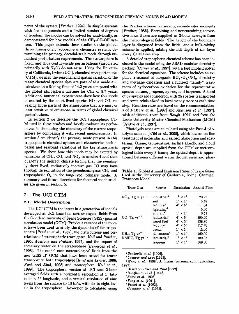
Figure 2. Monthly-mean modeled (solid lines) and observed (dots) mixing ratios of CO at surface measurement sites. All observational data are from Novelli et al. [1992], except for Cuiba [Kirchhoff et al., 1989].


Monthly-mean surface mixing ratios of ozone are shown in Figure 1; the solid lines represent modeled values, and the dots are mean mixing ratios over a number of years for selected measurement stations collated by Logan [1999]. The distribution and seasonality of ozone are reproduced well in tropical and equatorial regions, but the agreement is less good at higher latitudes in each hemisphere, where there is a tendency to overpredict the surface concentrations, particularly in spring when the cross-tropopause flux is at a maximum. Al- though use of the Synoz tracer allows the total flux of ozone into the troposphere to be well constrained, the * ...... ] and spatial ,rar;o*;•,• of the flux ;• •;,,• by transport in the tropopause region, and this is appar- ently too great in polar regions in the meteorological fields used. A separate problem, the overestimation of ozone concentrations by about 10-15 ppbv in continen- tal Europe, is probably due to the lack of a sub-grid- scale treatment of urban plumes, which leads to overestimation of the chemical ozone production efficiency per molecule of NOz [e.g., Jacob et al., 1993].

The distribution and seasonality of (JO are relatively well reproduced by the model, as shown in Figure 2. The high-latitude discrepancies seen in the ozone distribution are less pronounced here due to the negligible contribution of stratospheric air to CO abundance. The

measurements at Mace Head, Ireland, are sensitive to meteorological differences between the GISS fields and the real climate because of the position of the site immediately to the west of major European sources. Cui- ba, in the Amazon rain forest, sees extremely high CO mixing ratios in the spring due to biomass burning, and though the CO concentrations modeled at the peak of the burning season are rather low, as would be expected at the coarse resolution used in these studies, the seasonality of burning is well reproduced.

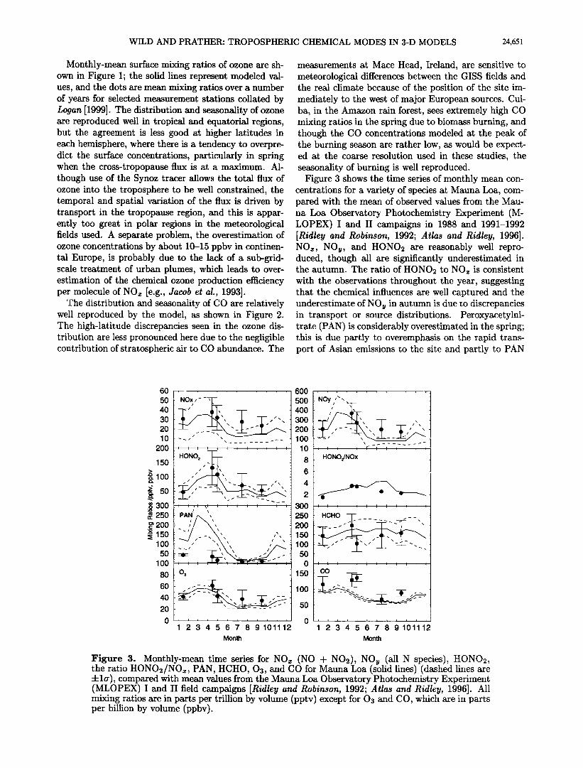
Figure 3 shows the time series of monthly mean concentrations for a variety of species at Mauna Loa, com- •J with the mean n• r•hq•rv•r] v•l,,•.• [rr•rn the Mau-

na Loa Observatory Photochemistry Experiment (M- LOPEX) I and II campaigns in 1988 and 1991-1992 [Ridley and Robinson, 1992; Atlas and Ridley, 1996]. NOx, NOy, and HONO2 are reasonably well reproduced, though all are significantly underestimated in the autumn. The ratio of HONO2 to NO• is consistent with the observations throughout the year, suggesting that the chemical influences are well captured and the underestimate of NOy in autumn is due •o discrepancies in transport or source distributions. Peroxyacetylni- trate (PAN) is considerably overestimated in the spring; this is due partly to overemphasis on the rapid transport of Asian emissions to the site and partly to PAN

60

50

40

30

20

10

200

150

100 { 5o o 300

• 250 • 200

._

.x_ :• 150

100

50

100

80

60

40

20

0

Month

6OO

5OO

4OO

3OO

2OO

IO0

10

8

6

4

2

3OO

25O

:00

5O

O0

5O

0

50

O0

50

t I I I I I I I { I I I

...• '• • /- --

I I t t t i t I I i i I

co

1 2 3 4 5 6 7 8 9 101112

Month

Figure 3. Monthly-mean time series for NOx (NO + NO•), NOy (all N species), HONOr, the ratio HONO•/NO•, PAN, HCHO, O•, and CO for Mauna Loa (solid lines) (dashed lines are :kla), compared with mean values from the Mauna Loa Observatory Photochemistry Experiment (MLOPEX) I and II field campaigns [Ridley and Robinson, 1992; Atlas and Ridley, 1996]. All mixing ratios are in parts per trillion by volume (pptv) except for O• and CO, which are in parts per billion by volume (ppbv).


t2 12[

10

Summer ..... -• Winter

0 100 200 300 400 500 600 700 800 0 100 200 300 400 500 600

PAN Mixing Ratio /pptv PAN Mixing Ratio /pptv 70O t00

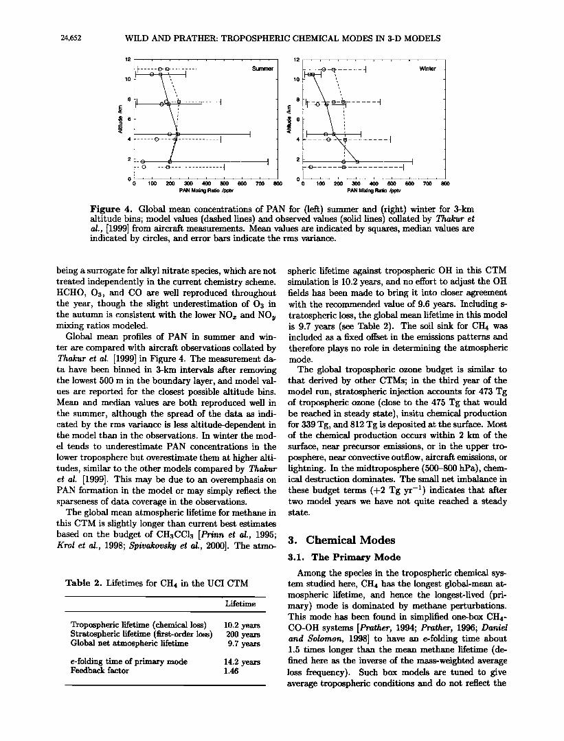
Figure 4. Global mean concentrations of PAN for (left) summer and (right) winter for 3-kin altitude bins; model values (dashed lines) and observed values (solid lines) collated by Thakur et al., [1999] from aircraft measurements. Mean values axe indicated by squares, median values are indicated by circles, and error bars indicate the rms vaxiance.

being a surrogate for alkyl nitrate species, which axe not treated independently in the current chemistry scheme. HCHO, 03, and CO are well reproduced throughout the year, though the slight underestimation of O3 in the autumn is consistent with the lower NOx and NOy mixing ratios modeled.

Global mean profiles of PAN in summer and winter are compared with aircraft observations collated by Thakur et al. [1999] in Figure 4. The measurement data have been binned in 3-km intervals after removing the lowest 500 m in the boundary layer, and model values are reported for the closest possible altitude bins. Mean and median values axe both reproduced well in the summer, although the spread of the data as indicated by the rms vaxiance is less altitude-dependent in the model than in the observations. In winter the model tends to underestimate PAN concentrations in the

lower troposphere but overestimate them at higher alti- tudes, similar to the other models compaxed by Thakur et al. [1999]. This may be due to an overemphasis on PAN formation in the model or may simply reflect the sparseness of data coverage in the observations.

The global mean atmospheric lifetime for methane in this CTM is slightly longer than current best estimates based on the budget of CH3CCI3 [Prinn et al., 1995; Krol et al., 1998; $pivakovsky et al., 2000]. The atmo-

Table 2. Lifetimes for CH4 in the UCI CTM

Lifetime

Tropospheric lifetime (chemical loss) Stratospheric lifetime (first-order loss) Global net atmospheric lifetime

e-folding time of primary mode Feedback factor

10.2 years 200 years 9.7 years

14.2 years 1.46

spheric lifetime against tropospheric OH in this CTM simulation is 10.2 years, and no effort to adjust the OH fields has been made to bring it into closer agreement with the recommended value of 9.6 yeaxs. Including s- tratospheric loss, the global mean lifetime in this model is 9.7 years (see Table 2). The soil sink for CH4 was included as a fixed offset in the emissions patterns and therefore plays no role in determining the atmospheric mode.

The global tropospheric ozone budget is similax to that derived by other CTMs; in the third year of the model run, stratospheric injection accounts for 473 Tg of tropospheric ozone (close to the 475 Tg that would be reached in steady state), insitu chemical production for 339 Tg, and 812 Tg is deposited at the surface. Most of the chemical production occurs within 2 km of the surface, neax precursor emissions, or in the upper troposphere, near convective outflow, aircraft emissions, or lightning. In the midtroposphere (500-800 hPa), chemical destruction dominates. The small net imbalance in

these budget terms (+2 Tg yr -1) indicates that after two model years we have not quite reached a steady state.

3. Chemical Modes

3.1. The Primary Mode

Among the species in the tropospheric chemical system studied here, CH4 has the longest global-mean atmospheric lifetime, and hence the longest-lived (primary) mode is dominated by methane perturbations. This mode has been found in simplified one-box CH4- CO-OH systems [Prather, 1994; Prather, 1996; Daniel and Solomon, 1998] to have an e-folding time about 1.5 times longer than the mean methane lifetime (defined here as the inverse of the mass-weighted average loss frequency). Such box models axe tuned to give average tropospheric conditions and do not reflect the


lOO

• o

ß CH 4

. • CO

.

, i :I. i i i i i i i i

80

60

40

20

o

3.0

2.0

1.0

0.5

0

-5.0e-4

-1.0e-3

-1.5e-3

-2.0e-3 0 1 2 3 4 5 6 7 8 9 10

Emissions Year of Run Period

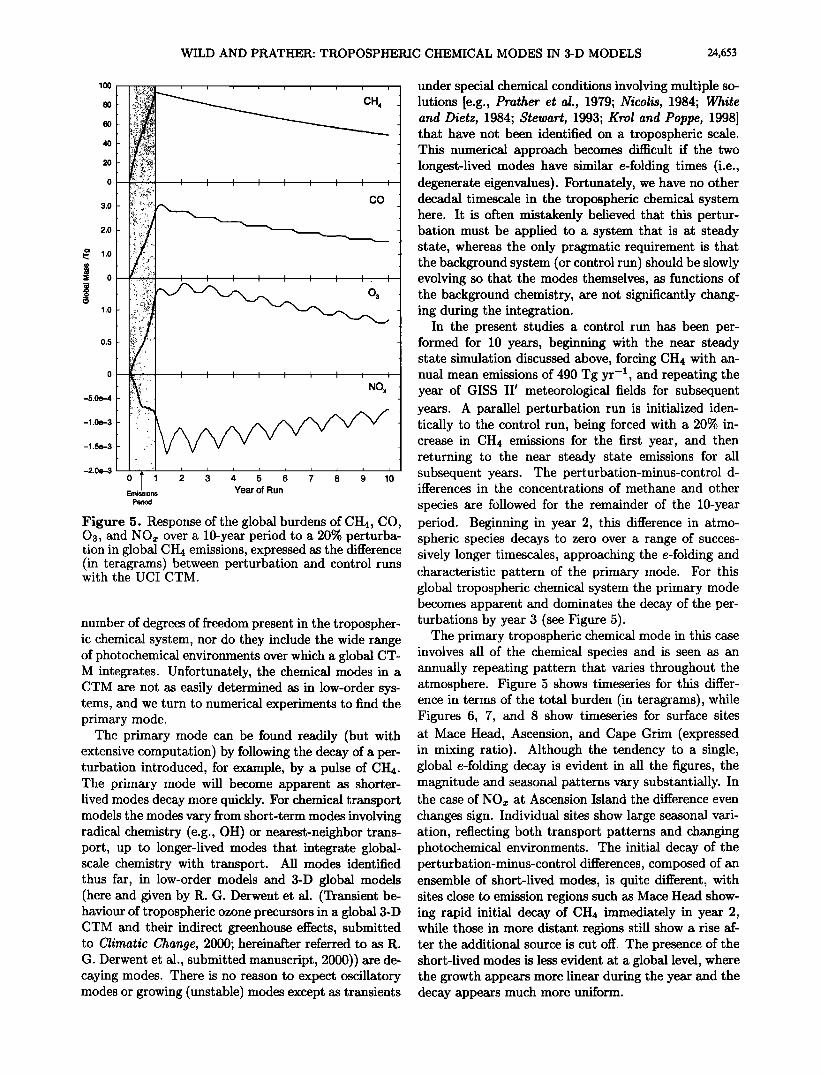
Figure 5. Response of the global burdens of CH4, CO, Oa, and NOx over a 10-year period to a 20% perturbation in global CH4 emissions, expressed as the difference (in teragrams) between perturbation and control runs with the U CI CTM.

number of degrees of freedom present in the tropospheric chemical system, nor do they include the wide range of photochemical environments over which a global CT- M integrates. Unfortunately, the chemical modes in a CTM are not as easily determined as in low-order systems, and we turn to numerical experiments to find the primary mode.

The primary mode can be found readily (but with extensive computation) by following the decay of a perturbation introduced, for example, by a pulse of CH4. /'1-• 1 .11

zne primary mode wm become apparent as shorter- lived modes decay more quickly. For chemical transport models the modes vary from short-term modes involving radical chemistry (e.g., OH) or nearest-neighbor transport, up to longer-lived modes that integrate global- scale chemistry with transport. All modes identified thus far, in low-order models and 3-D global models (here and given by R. G. Derwent et al. (Transient be- haviour of tropospheric ozone precursors in a global 3-D CTM and their indirect greenhouse effects, submitted to Climatic Change, 2000; hereinafter referred to as R. G. Derwent et al., submitted manuscript, 2000)) are decaying modes. There is no reason to expect oscillatory modes or growing (unstable) modes except as transients

under special chemical conditions involving multiple solutions [e.g., Prather et al., 1979; Nicolis, 1984; White and Dietz, 1984; Stewart, !993; Krol and Poppe, 1998] that have not been identified on a tropospheric scale. This numerical approach becomes difficult if the two longest-lived modes have similar e-folding times (i.e., degenerate eigenvalues). Fortunately, we have no other decadal timescale in the tropospheric chemical system here. It is often mistakenly believed that this perturbation must be applied to a system that is at steady state, whereas the only pragmatic requirement is that the background system (or control run) should be slowly evolving so that the modes themselves, as functions of the background chemistry, are not significantly changing during the integration.

In the present studies a control run has been per- formed for 10 years, beginning with the near steady state simulation discussed above, forcing CH4 with annual mean emissions of 490 Tg yr -•, and repeating the year of GISS IY meteorological fields for subsequent years. A parallel perturbation run is initialized iden- tically to the control run, being forced with a 20% increase in CH4 emissions for the first year, and then returning to the near steady state emissions for all subsequent years. The perturbation-minus-control d- ifferences in the concentrations of methane and other

species are followed for the remainder of the 10-year period. Beginning in year 2, this difference in atmospheric species decays to zero over a range of succes- sively longer timescales, approaching the e-folding and characteristic pattern of the primary mode. For this global tropospheric chemical system the primary mode becomes apparent and dominates the decay of the perturbations by year 3 (see Figure 5).

The primary tropospheric chemical mode in this case involves all of the chemical species and is seen as an annually repeating pattern that varies throughout the atmosphere. Figure 5 shows timeseries for this difference in terms of the total burden (in teragrams), while Figures 6, 7, and 8 show timeseries for surface sites at Mace Head, Ascension, and Cape Grim (expressed in mixing ratio). Although the tendency to a single, global e-folding decay is evident in all the figures, the

the case of NOx at Ascension Island the difference even changes sign. Individual sites show large seasonal variation, reflecting both transport patterns and changing photochemical environments. The initial decay of the perturbation-minus-control differences, composed of an ensemble of short-lived modes, is quite different, with sites close to emission regions such as Mace Head showing rapid initial decay of CH4 immediately in year 2, while those in more distant regions still show a rise after the additional source is cut off. The presence of the short-lived modes is less evident at a global level, where the growth appears more linear during the year and the decay appears much more uniform.


80

70

60

50

40

3O

20

10

0

1.0

0.8

0.6

0.4

• 0.2 o

,e 0

•_• 0.20

0.15

0.10

0.05

0

0

-0.001

-0.002

-0.003

-0.004

-0.005 0 I 2 3 4 5 6 7 8 9 10


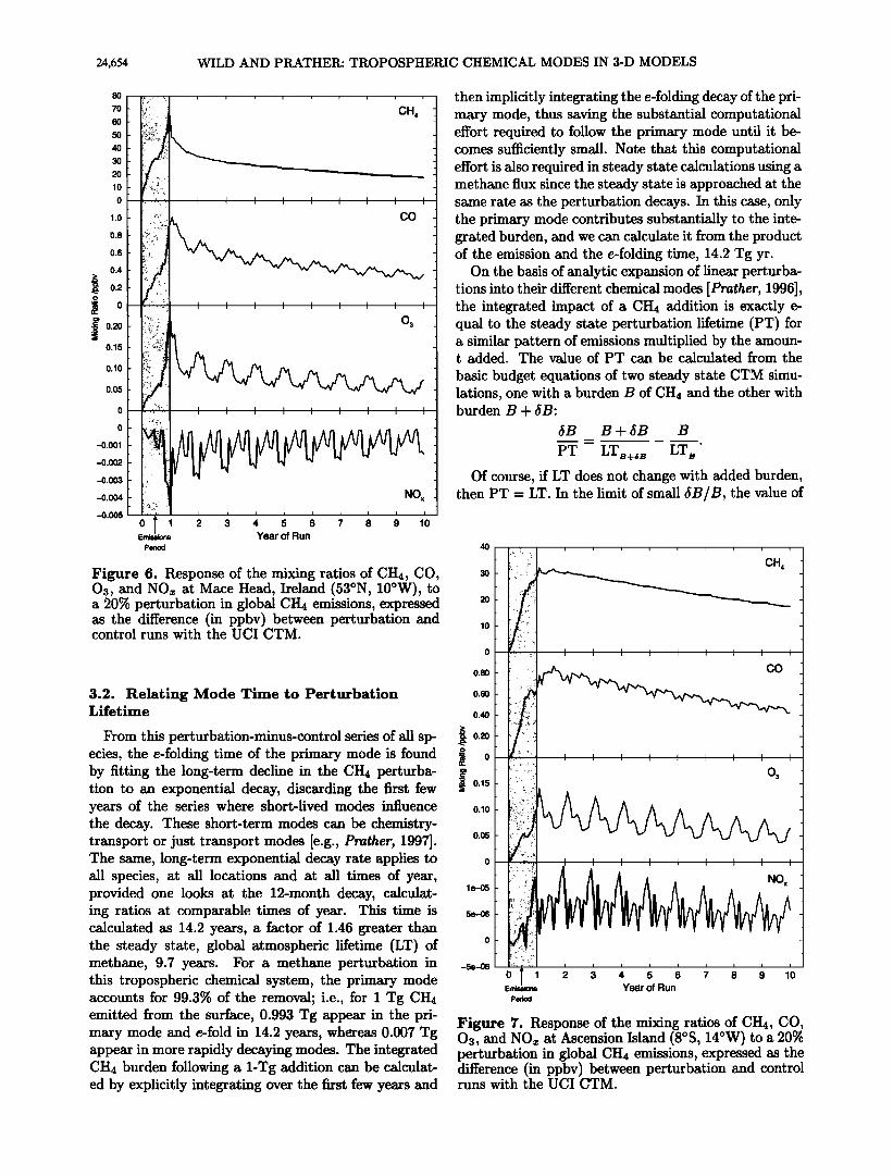
Figure 6. Response of the mixing ratios of CH4, CO, 03, and NOx at Mace Head, Ireland (53øN, 10øW), to a 20% perturbation in global CH4 emissions, expressed as the difference (in ppbv) between perturbation and control runs with the U CI CTM.

3.2. Relating Mode Time to Perturbation Lifetime

From this perturbation-minus-control series of all species, the e-folding time of the primary mode is found by fitting the long-term decline in the CH4 perturbation to an exponential decay, discarding the first few years of the series where short-lived modes influence the decay. These short-term modes can be chemistry- transport or just transport modes [e.g., Prather, 1997]. The same, long-term exponential decay rate applies to all species, at all locations and at all times of year, provided one looks at the 12-month decay, calculating ratios at comparable times of year. This time is calculated as 14.2 years, a factor of 1.46 greater than the steady state, global atmospheric lifetime (LT) of methane, 9.7 years. For a methane perturbation in this tropospheric chemical system, the primary mode accounts for 99.3% of the removal; i.e., for I Tg CH4 emitted from the surface, 0.993 Tg appear in the primary mode and e-fold in 14.2 years, whereas 0.007 Tg appear in more rapidly decaying modes. The integrated CH4 burden following a 1-Tg addition can be calculated by explicitly integrating over the first few years and

then implicitly integrating the e-folding decay of the primary mode, thus saving the substantial computational effort required to follow the primary mode until it becomes sufficiently small. Note that this computational effort is also required in steady state calculations using a methane flux since the steady state is approached at the same rate as the perturbation decays. In this case, only the primary mode contributes substantially to the integrated burden, and we can calculate it from the product of the emission and the e-folding time, 14.2 Tg yr.

On the basis of analytic expansion of linear perturbations into their different chemical modes [Prather, 1996], the integrated impact of a CH4 addition is exactly e- qual to the steady state perturbation lifetime (PT) for a similar pattern of emissions multiplied by the amoun- t added. The value of PT can be calculated from the

basic budget equations of two steady state CTM simulations, one with a burden B of CH4 and the other with burden B + 5B'

5B B + 5B B

PT LT•+• LT• Of course, if LT does not change with added burden,

then PT - LT. In the limit of small jB/B, the value of

4O

3O

20

10

0

0.80

0.60

0.40

'•. 0.20

• o

x 0.15

0.10

0.05

0

I e-05

0

-5e-06 0 1 2 3 4 5 6


7 8 9 10

Figure ?. Response of the mixing ratios of CH4, CO, Os, and NO• at Ascension Island (8øS, 14øW) to a 20% perturbation in global CH4 emissions, expressed as the difference (in ppbv) between perturbation and control runs with the UCI CTM.


2O

0

0.80

0.60

0.40

• 0.20

{ o

.•- 0.15

0.10

0.05

0

1 e-04

-le-04

-2e -04

0 T 1 2 3 4 5 6 7 8 9 10 Emjss•ns Year of Run

Period

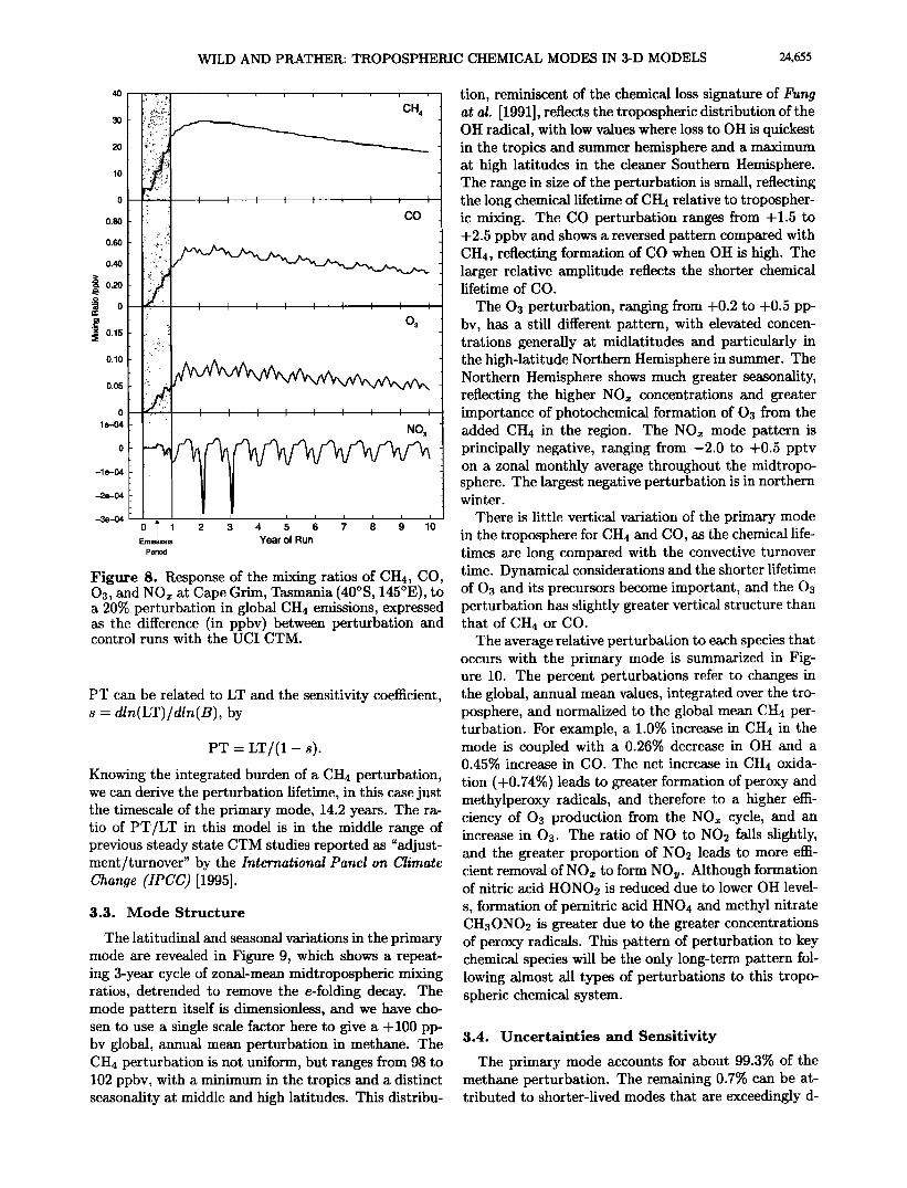
Figure 8. Response of the mixing ratios of CH4, CO, 03, and NOx at Cape Grim, Tasmania (40øS, 145øE), to a 20% perturbation in global CH4 emissions, expressed as the difference (in ppbv) between perturbation and control runs with the U CI CTM.

PT can be related to LT and the sensitivity coefficient, s - dln(LT)/dln(B), by

PT- LT/(1 - s).

Knowing the integrated burden of a CH4 perturbation, we can derive the perturbation lifetime, in this case just the timescale of the primary mode, 14.2 years. The ratio of PT/LT in this model is in the middle range of previous steady state CTM studies reported as "adjust-

Chage (IPCC) [1995].

3.3. Mode Structure

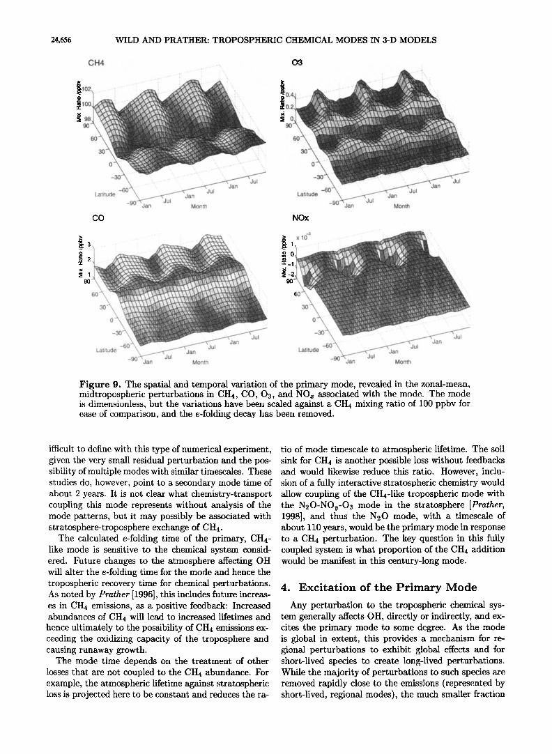
The latitudinal and seasonal variations in the primary mode are revealed in Figure 9, which shows a repeating 3-year cycle of zonal-mean midtropospheric mixing ratios, detrended to remove the e-folding decay. The mode pattern itself is dimensionless, and we have cho- sen to use a single scale factor here to give a +100 ppbv global, annual mean perturbation in methane. The CH4 perturbation is not uniform, but ranges from 98 to 102 ppbv, with a minimum in the tropics and a distinct seasonality at middle and high latitudes. This distribu-

tion, reminiscent of the chemical loss signature of Fung at al. [1991], reflects the tropospheric distribution of the OH radical, with low values where loss to OH is quickest in the tropics and summer hemisphere and a maximum at high latitudes in the cleaner Southern Hemisphere. The range in size of the perturbation is small, reflecting the long chemical lifetime of CH4 relative to tropospheric mixing. The CO perturbation ranges from +1.5 to +2.5 ppbv and shows a reversed pattern compared with CH4, reflecting formation of CO when OH is high. The larger relative amplitude reflects the shorter chemical lifetime of CO.

The 03 perturbation, ranging from +0.2 to +0.5 pp- by, has a still different pattern, with elevated concentrations generally at midlatitudes and particularly in the high-latitude Northern Hemisphere in summer. The Northern Hemisphere shows much greater seasonality, reflecting the higher N Ox concentrations and greater importance of photochemical formation of 03 from the added CH4 in the region. The N Ox mode pattern is principally negative, ranging from -2.0 to +0.5 pptv on a zonal monthly average throughout the midtroposphere. The largest negative perturbation is in northern winter.

There is little vertical variation of the primary mode in the troposphere for CH4 and CO, as the chemical lifetimes are long compared with the convective turnover time. Dynamical considerations and the shorter lifetime of 03 and its precursors become important, and the 03 perturbation has slightly greater vertical structure than that of CH4 or CO.

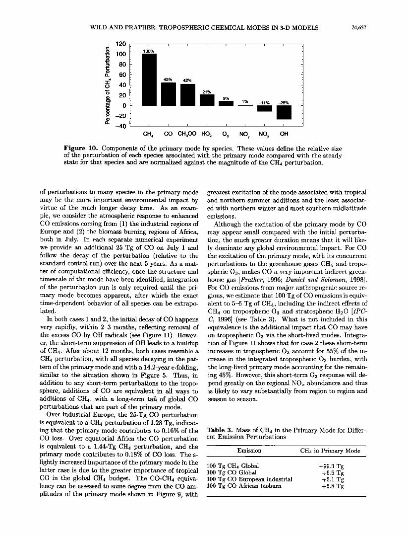
The average relative perturbation to each species that occurs with the primary mode is summarized in Fig- ure 10. The percent perturbations refer to changes in the global, annual mean values, integrated over the troposphere, and normalized to the global mean CH4 perturbation. For example, a 1.0% increase in CH4 in the mode is coupled with a 0.26% decrease in OH and a 0.45% increase in CO. The net increase in CH4 oxida-

tion (+0.74%) leads to greater formation of peroxy and methylperoxy radicals, and therefore to a higher efficiency of 03 production from the NO• cycle, and an increase in 03. The ratio of NO to NO2 falls slightly, and the greater proportion of NO2 leads to more effi- cient removal of NOz to form NO u. Although formation of nitric acid HONO2 is reduced due to lower OH level- s, formation of pernitric acid HNO4 and methyl nitrate CH3ONO2 is greater due to the greater concentrations of peroxy radicals. This pattern of perturbation to key chemical species will be the only long-term pattern following almost all types of perturbations to this tropospheric chemical system.

3.4. Uncertainties and Sensitivity

The primary mode accounts for about 99.3% of the methane perturbation. The remaining 0.7% can be at- tributed to shorter-lived modes that are exceedingly d-


CH4 .. ,, 03

100 •¾' • ........ •:.?....•-;,½•:ii:•-,.,•-:•. :':•-:..•',•.• ....... .•%•-[ •,

0 '• • • •".? '.' ...... ß ' • ß ' ß

-90 Jan Jul -90 Jan Jut Month Month CO NOx

Latitude Jul

-90 jan•• •Jul Jan Month

-3

• x 10 • 1 ._o 0

•-1

9O

Latitude

• 'Jan

\ •..•"••a• 'Jut -90 Jan Jul Month

Figure 9. The spatial and temporal variation of the primary mode, revealed in the zonal-mean, midtropospheric perturbations in CH4, CO, 03, and NOx associated with the mode. The mode is dimensionless, but the variations have been scaled against a CH4 mixing ratio of 100 ppbv for ease of comparison, and the e-folding decay has been removed.

ifficult to define with this type of numerical experiment, given the very small residual perturbation and the possibility of multiple modes with similar timescales. These studies do, however, point to a secondary mode time of about 2 years. It is not clear what chemistry-transport coupling this mode represents without analysis of the mode patterns, but it may possibly be associated with stratosphere-troposphere exchange of CH4.

The calculated e-folding time of the primary, CH4- like mode is sensitive to the chemical system considered. Future changes to the atmosphere affecting OH will alter the e-folding time for the mode and hence the tropospheric recovery time for chemical perturbations. As noted by Prather [1996], this includes future increases in CH4 emissions, as a positive feedback: Increased abundances of CH4 will lead to increased lifetimes and hence ultimately to the possibility of CH4 emissions ex- ceeding the oxidizing capacity of the troposphere and causing runaway growth.

The mode time depends on the treatment of other losses that are not coupled to the CH4 abundance. For example, the atmospheric lifetime against stratospheric loss is projected here to be constant and reduces the ra-

tio of mode timescale to atmospheric lifetime. The soil sink for CH4 is another possible loss without feedbacks and would likewise reduce this ratio. However, inclu- sion of a fully interactive stratospheric chemistry would allow coupling of the CH4-1ike tropospheric mode with the N20-NOy-03 mode in the stratosphere [Prather, 1998], and thus the N20 mode, with a timescale of about 110 years, would be the primary mode in response to a CH4 perturbation. The key question in this fully coupled system is what proportion of the CH4 addition would be manifest in this century-long mode.

4. Excitation of the Primary Mode

Any perturbation to the tropospheric chemical system generally affects OH, directly or indirectly, and ex- cites the primary mode to some degree. As the mode is global in extent, this provides a mechanism for regional perturbations to exhibit global effects and for short-lived species to create long-lived perturbations. While the majority of perturbations to such species are removed rapidly close to the emissions (represented by short-lived, regional modes), the much smaller fraction


120

lOO 80

60

40

20

o

-20

-40

45% 42%

21%

9%

• 1% - 11% -26%

CH 4 CO CH3OO HO 2 0 3 NOy NO x OH

Figure 10. Components of the primary mode by species. These values define the relative size of the perturbation of each species associated with the primary mode compared with the steady state for that species and are normalized against the magnitude of the CH4 perturbation.

of perturbations to many species in the primary mode may be the more important environmental impact by virtue of the much longer decay time. As an example, we consider the atmospheric response to enhanced CO emissions coming from (1) the industrial regions of Europe and (2) the biomass burning regions of Africa, both in July. In each separate numerical experiment we provide an additional 25 Tg of CO on July 1 and follow the decay of the perturbation (relative to the standard control run) over the next 5 years. As a mat- ter of computational efficiency, once the structure and timescale of the mode have been identified, integration of the perturbation run is only required until the primary mode becomes apparent, after which the exact time-dependent behavior of all species can be extrapo- lated.

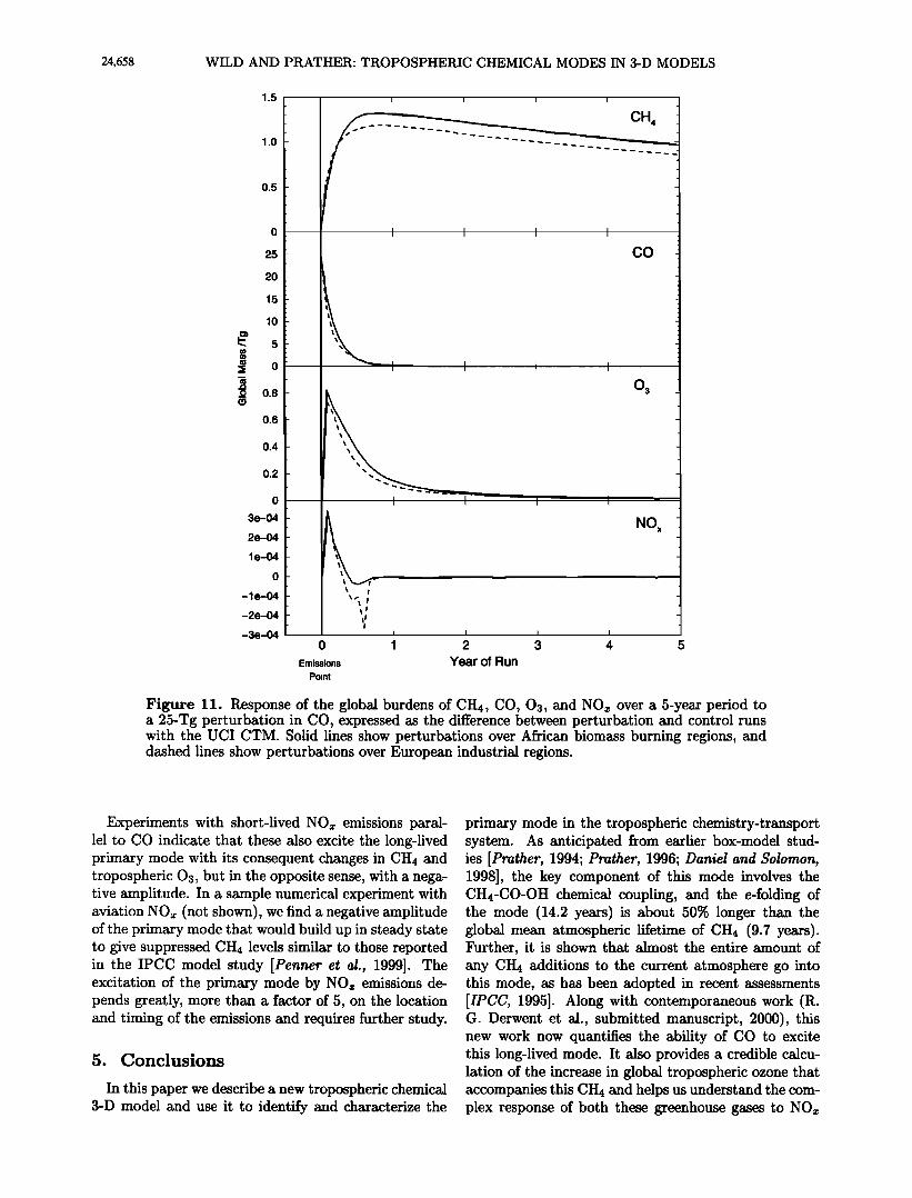
In both cases 1 and 2, the initial decay of CO happens very rapidly, within 2-3 months, reflecting removal of the excess CO by OH radicals (see Figure 11). Howev- er, the short-term suppression of OH leads to a buildup of CH4. After about 12 months, both cases resemble a CH4 perturbation, with all species decaying in the pattern of the primary mode and with a 14.2-year e-folding, similar to the situation shown in Figure 5. Thus, in addition to any short-term perturbations to the troposphere, additions of CO are equivalent in all ways to additions of CH4, with a long-term tail of global CO perturbations that are part of the primary mode.

Over industrial Europe, the 25-Tg CO perturbation is equivalent to a CH4 perturbation of 1.28 Tg, indicat- ing that the primary mode contributes to 0.16% of the CO loss. Over equatorial Africa the CO perturbation is equivalent to a 1.44-Tg CH4 perturbation, and the primary mode contributes to 0.18% of CO loss. The s- lightly increased importance of the primary mode in the latter case is due to the greater importance of tropical CO in the global CH4 budget. The CO-CH4 equiva- lency can be assessed to some degree from the CO amplitudes of the primary mode shown in Figure 9, with

greatest excitation of the mode associated with tropical and northern summer additions and the least associat-

ed with northern winter and most southern midlatitude

emissions.

Although the excitation of the primary mode by CO may appear small compared with the initial perturbation, the much greater duration means that it will likely dominate any global environmental impact. For CO the excitation of the primary mode, with its concurrent perturbations to the greenhouse gases CH4 and tropospheric 03, makes CO a very important indirect greenhouse gas [Prather, 1996; Daniel and Solomon, 1998]. For CO emissions from major anthropogenic source regions, we estimate that 100 Tg of CO emissions is equivalent to 5-6 Tg of CH4, including the indirect effects of CH4 on tropospheric 03 and stratospheric H20 [IPC- C, 1996] (see Table 3). What is not included in this equivalence is the additional impact that CO may have on tropospheric 03 via the short-lived modes. Integra- tion of Figure 11 shows that for case 2 these short-term increases in tropospheric 03 account for 55% of the increase in the integrated tropospheric 03 burden, with the long-lived primary mode accounting for the remaining 45%. However, this short-term 03 response will de- pend greatly on the regional N Ox abundances and thus is likely to vary substantially from region to region and season to season.

Table 3. Mass of CH4 in the Primary Mode for Differ- ent Emission Perturbations

Emission CH4 in Primary Mode

100 Tg CH4 Global 100 Tg CO Global 100 Tg CO European industrial 100 Tg CO African bioburn

+99.3 Tg +5.5 Tg +5.1 Tg +5.8 Tg


1.5

1.0

0.5

o

25

20

15

lO

e: 5

• 0

._o 0.8

0.6

0.4

0.2

0

3e-04

2e-04

le-04

0

-le-04

-2e-04

-3e-04 0 1 2 3 4 5

Emissions Year of Run Point

Figure 11. Response of the global burdens of CH4, CO, 03, and NOx over a 5-year period to a 25-Tg perturbation in CO, expressed as the difference between perturbation and control runs with the U CI CTM. Solid lines show perturbations over African biomass burning regions, and dashed lines show perturbations over European industrial regions.

Experiments with short-lived NOx emissions parallel to CO indicate that these also excite the long-lived primary mode with its consequent changes in CH4 and tropospheric 03, but in the opposite sense, with a negative amplitude. In a sample numerical experiment with aviation NO• (not shown), we find a negative amplitude of the primary mode that would build up in steady state to give suppressed CH4 levels similar to those reported in the IPCC model study [Penner et al., 1999]. The excitation of the primary mode by NO• emissions depends greatly, more than a factor of 5, on the location and timing of the emissions and requires further study.

5. Conclusions

In this paper we describe a new tropospheric chemical 3-D model and use it to identify and characterize the

primary mode in the tropospheric chemistry-transport system. As anticipated from earlier box-model studies [Prather, 1994; Prather, 1996; Daniel and Solomon, 1998], the key component of this mode involves the CHa-CO-OH chemical coupling, and the e-folding of the mode (14.2 years) is about 50% longer than the global mean atmospheric lifetime of CH4 (9.7 years). Further, it is shown that almost the entire amount of any CH4 additions to the current atmosphere go into this mode, as has been adopted in recent assessments [IPCC, 1995]. Along with contemporaneous work (R. G. Derwent et al., submitted manuscript, 2000), this new work now quantifies the ability of CO to excite this long-lived mode. It also provides a credible calculation of the increase in global tropospheric ozone that accompanies this CH4 and helps us understand the com- plex response of both these greenhouse gases to NO•


additions as shown in the recent international aviation

assessment [Penner et al., 1999]. Modes are a natural property of the atmospheric

chemical system, and as such they exist in the real atmosphere as well as in the simplified system of a CTM. However, they will not be easy to discern, because interannual variability in atmospheric circulation will slightly alter the year-to-year patterns and because the constant variation in the terrestrial sources of trace gases provides continual excitation of the full range of modes. In addition, coupling of the tropospheric chemical system with stratospheric chemistry through the effects of CH4 on stratospheric O3 and thence on N20 and tropospheric UV will lead to the presence of a century-scale mode. Nevertheless, the long-lived CH4-1ike mode is expected to dominate the tropospheric system and may provide an important tool for assessing the impact that mankind has, and will continue to have, on the atmosphere.

Acknowledgments. This research was supported through grants to UCI from the Atmospheric Chemistry Pro- grams of the NSF and NASA, the Atmospheric Effects of Aviation Program of NASA, and the Chemistry and Circu- lation Occultation Spectroscopy Investigation from NASA. The authors thank the two reviewers for their careful read-

ing of the manuscript.

References

Atkinson, R., D.L. Baulch, R.A. Cox, R.F. Hampson, J.A. Kerr, M.J. Rossi, and J. Troe, Evaluated kinetic, photochemical and heterogeneous data for atmospheric chemistry: Supplement V, IUPAC subcommittee on gas kinetic data evaluation for atmospheric chemistry, J. Phys. Chem. Reft Data, 26, 521-1011, 1997.

Atlas, E.L., and B.A. Ridley, The Mauna Loa Observatory Photochemistry Experiment: Introduction, J. Geophys. Res., 101, 14,531-14,541, 1996.

Availone, L.M., and M.J. Prather, Tracer-tracer correlation- s: Three-dimensional model simulations and comparisons to observations, J. Geophys. Res., 102, 19,233-19,246, 1997.

Balkanski, Y.J., D.J. Jacob, G.M. Gardiner, W.C. Grau- stein, and K.K. Turekian, Transport and residence times of tropospheric aerosols inferred from a global three-dimensional simulation of 210-Pb, J. Geophys. Res., 98, 20,573-20,586, 1993.

Bates, T.S., K.C. Kelly, J.E. Johnson, and R.H. Gammon, Regional and seasonal variations in the flux of oceanic carbon monoxide to the atmosphere, J. Geophys. Res., 100, 23,093-23,101, 1995.

Baughcum, S.L., T.G. Tritz, S.C. Henderson, and D.C. Pick- ett, Scheduled civil aircraft emission inventories for 1992: Database development and ana!ysis, NASA CR-J 700, 72 pp., 1996. .•, •

Benkovitz, C.M., M.T. Scholtz, J. Pacyna, L. Tarrason, J. Dignon, E.C. Voldner, P.A. Spiro, J.A. Logan, and T.E. Graedel, Global gridded inventories of anthropogenic e- missions of sulfur and nitrogen, J. Geophys. Res., 101, 29,239-29,253, 1996.

Carver, G.D., P.D. Brown, and O. Wild, The ASAD atmospheric chemistry integration package and chemical reaction database, Cornput. Phys. Commun., 105, 197-215, 1997.

Daniel, J. S., and S. Solomon, On the climate forcing of carbon monoxide, J. Geophys. Res., 103, 13,249-13,260, 1998.

DeMore, W.B., S.P. Sander, D.M. Golden, R.F. Hampson, M.J. Kurylo, C.J. Howard, A.R. Ravishankara, C.E. Kolb, and M.J. Molina, Chemical kinetics and photochemical data for use in stratospheric modeling, JPL Publ. 97-J, 269 pp., 1997.

Fung, I., J. John, J. Lerner, E. Matthews, M. Prather, L.P. Steele, and P.J. Fraser, Three-dimensional model synthe- sis of the global methane cycle, J. Geophys. Res., 96, 13,033-13,065, 1991.

Guenther, A., et al., A global model of natural volatile organic compound emissions, J. Geophys. Res., 100, 8873- 8892, 1995.

Hall, T.M., and M.J. Prather, Seasonal evolution of N20, 03, and CO2: Three-dimensional simulations of stratospheric correlations, J. Geophys. Res., 100, 16,699-16,720, 1995.

Hall, T.M., D.W. Waugh, K.A. Boering, and R.A. Plumb, Evaluation of transport in stratospheric models, J. Geo- phys. Res, 10•, 18,815-18,839, 1999.

Hannegan, B., S. Olsen, M. Prather, X. Zhu, D. Rind, and J. Lerner, The dry stratosphere: A limit on cometary water influx, Geophys. Res. Left., 25, 1649-1652, 1998.

Hough, A.M., Development of a two-dimensional global tropospheric model: Model chemistry, J. Geophys. Res., 96, 7325-7362, 1991.

International Panel on Climate Change, Climate Change 199•{: Radiative Forcing of Climate Change and an E- valuation of the IPCC IS9œ Emission Scenarios, edited by J. T. Houghton et al., Cambridge Univ. Press, New York, 1995.

International Panel on Climate Change, Climate Change 1995: The Science of Climate Change, edited by J. T. Houghton et al., Cambridge Univ. Press, New York, 1996.

Isaksen, I.S.A., O. Hov, S.A. Penkett, and A. Semb, Model analysis of the measured concentration of organic gases in the Norwegian Arctic, J. Atmos. Chem., 3, 3-27, 1985.

Jacob, D.J., J.A. Logan, G.M. Gardner, R.M. Yevich, C.M. Spivakovsky, and S.C. Wofsy, Factors regulating ozone over the United States and its export to the global atmosphere, J. Geophys. Res., 98, 14,817-14,826, 1993.

Jenkin, M.E., S.M. Saunders, and M.J. Pilling, The tropospheric degradation of volatile organic compounds: A protocol for mechanism development, Atmos. Environ., 31, 81-104, 1997.

Kirchhoff, V.W.K.H., and R.A. Rasmussen, Time variations of CO and ozone concentrations in a region subject to biomass burning, J. Geophys. Res., 95, 7521-7532, 1990.

Kirchhoff, V.W.K.H., A.W. Setzer, and M.C. Peteira, Biom- ass burning in Amazonia: Seasonal effects on atmospheric O3 and CO, Geophys. Res. Left., 16, 469-472, 1989.

Koch, D., and D. Rind, XøBe/7Be as a tracer of stratospheric transport, J. Geophys. Res., 103, 3907-3917, 1998.

Krol, M., and D. Poppe, Nonlinear dynamics in atmospheric chemistry rate equations, J. Atmos. Chem., 29, 1-16, 1998.

Krol, M., P.J. van Leeuwen, and J. Lelieveld, Global OH trend inferred from methylchloroform measurements, J. Geophys. Res., 103, 10,697-10,711, 1998.

Law, K.S., and J.A. Pyle, Modeling trace gas budgets in the troposphere, 1, Ozone and odd nitrogen, J. Geophys. Res., 98, 18,377-18,400, 1993.

Logan, J. A., An analysis of ozonesonde data for the troposphere: Recommendations for testing 3-D models and development of a gridded climatology for tropospheric o- zone, J. Geophys. Res., 104, 16,115-16,149, 1999.

Logan, J.A., M.J. Prather, S.C. Wofsy, and M.B. McElroy,


Tropospheric chemistry: A global perspective, J. Geo- phys. Res., $6, 7210-7254, 1981.

Manning, M.R., Characteristic modes of isotopic variations in atmospheric chemistry, Geophys. Res. Left., 26, 1263- 1266, 1999.

Mathews, E., Global vegetation and land use: New high resolution data bases for climate studies, J. Clim. Appl. Meteorok, 22, 474-487, 1983.

McLinden, C.A., S. Olsen, B. Hannegan, O. Wild, M.J. Prather, and J. Sundet, Stratospheric ozone in three- dimensional models: A simple chemistry and the cross- tropopause flux, J. Geophys. Res., 105, 14,653-14,665, 2000.

Murphy, D.M., and D.W. Fahey, An estimate of the flux of stratospheric reactive nitrogen and ozone into the troposphere, J. Geophys. Res., 99, 5325-5332, 1994.

Nicolis, G., Bifurcations and symmetry-breaking in far- from-equilibrium systems -- Towards a dynamics of com- plexity, Adv. Chem. Phys., 55, 179-199, 1984.

Novelli, P.C., L.P. Steele, and P.P. Tans, Mixing ratios of carbon monoxide in the troposphere, J. Geophys. Res., 97, 20,731-20,750, 1992.

Oltmans, S. J., and H. Levy, Surface ozone measurements from a global network, Atmos. Environ., 28, 9-24, 1994.

Penner, J.E., D.H. Lister, D.J. Griggs, D.J. Dokken, and M. McFarland (Eds.), Aviation and the Global Atmosphere, 373 pp., Cambridge Univ. Press, New York, 1999.

Piccot, S.D., J.L. Watson, and J.W. Jones, A global inventory of volatile organic compound emissions from anthropogenic sources, J. Geophys. Res., 97, 9897-9912, 1992.

Prather, M. J., Numerical advection by conservation of second-order moments, J. Geophys. Res., 91, 6671-6681, 1986.

Prather, M.J., Lifetimes and eigenstates in atmospheric chemistry, Geophys. Res. Lett., 21, 801-804, 1994.

Prather, M. J., Timescales in atmospheric chemistry: The- ory, GWPs for CH4 and CO, and runaway growth, Geo- phys. Res. Left., 23, 2597-2600, 1996.

Prather, M. J., Timescales in atmospheric chemistry: CH3Br the ocean, and ozone depletion potentials, Global Bio- geochem. Cycles, 11, 393-400, 1997.

Prather, M. J., Timescales in atmospheric chemistry: Cou- pled perturbations to N20, NO v and 03, Science, 279, 1339-1341, 1998.

Prather, M.J., M.B. McElroy, and S.C. Wofsy, Stratospheric chemistry: Multiple solutions, Geophys. Res. Left., 6, 163-164, 1979.

Prather, M., M. McElroy, S. Wofsy, G. Russell, and D. Rind, Chemistry of the global troposphere: Fluorocarbons as tracers of air motion, J. Geophys. Res., 92, 6579-6613, 1987.

Price, C., and D. Rind, A simple lightning parameterization for calculating global lightning distributions, J. Geophys. Res., 97, 9919-9933, 1992.

Prinn, R.G., R.F. Weiss, B.R. Miller, J. Huang, F.N. Alyea, D.M. Cunnold, P.J. Fraser, D.E. Hartley, and P.G. Sim- monds, Atmospheric trends and lifetime of CH3CC13 and global OH concentrations, Science, 269, 187-192, 1995.

Ridley, B. A., and E. Robinson, The Mauna Loa Observa- tory Photochemistry Experiment, J. Geophys. Res., 97, 10,285-10,290, 1992.

Rind, D., and J. Lerner, Use of on-line tracers as a diagnostic tool in general circulation model development, 1, Horizontal and vertical transport in the troposphere, J. Geophys. Res., 101, 12,667-12,683, 1996.

Rind, D., J. Lerner, K. Shah, and R. Suozzo, Use of on-line tracers as a diagnostic tool in general circulation model development, 2, Transport between the troposphere and stratosphere, J. Geophys. Res., 10•, 9151-9167, 1999.

Spivakovsky, C.M., et al., Three-dimensional climatological distribution of tropospheric OH: Update and evaluation, J. Geophys. Res., 105, 8931-8980, 2000.

Stewart, R.W., Multiple steady states in atmospheric chemistry, J. Geophys. Res., 98, 20,601-20,611, 1993.

Thakur, A. N., H. B. Singh, P. Mariani, Y. Chen, Y. Wang, D. J. Jacob, G. Brasseur, J.-F. Mfiller, and M. Lawrence, Distribution of reactive nitrogen species in the remote free troposphere: Data and model comparisons, Atmos. Env- iron., 33, 1403-1422, 1999.

Wang, Y.H., D.J. Jacob, and J.A. Logan, Global simulation of tropospheric O3-NOx-hydrocarbon chemistry, 1, Model formulation, J. Geophys. Res., 103, 10,713-10,725, 1998.

White, W.H., and D. Dietz, Does the photochemistry of the troposphere admit more than one steady-state?, Nature, 309, 242-244, 1984.

Wild, O., X. Zhu, and M.J. Prather, Fast-J: Accurate simulation of in- and below-cloud photolysis in tropospheric chemical models, J. Atmos. Chem., in press, 2000.

Yienger, J.J., and H. Levy II, Empirical model of global soil- biogenic NOx emissions, J. Geophys. Res., 100, 11,447- 11,464, 1995.

M. J. Prather, Earth System Science, University of Cali- fornia, Irvine, Irvine, CA 92697. ([email protected])

O. Wild, Institute for Global Change Research (Yoko- hama), Frontier Research System for Global Change, 3173- 25 Showa-machi, Kanazawa-ku, Yokohama, Kanagawa 236- 0001, Japan. ([email protected])

(Received March 16, 2000; revised June 8, 2000; accepted June 29, 2000.)

excitation of the primary tropospheric chemical mode in...

Documents