GEOFIZIKA VOL. 35 2018

DOI: 10.15233/gfz.2018.35.11 Original scientific paper

Exchange of dense water between the open North Adriatic and the Croatian coastal sea:

Explicitly solving a nonlinear problem

Mirko Orlić

Andrija Mohorovičić Geophysical Institute, Department of Geophysics, Faculty of Science, University of Zagreb, Zagreb, Croatia

Received 26 June 2018, in final form 13 December 2018

It has been known for a while that there are two sites of wintertime dense water formation in the North Adriatic – one in the open sea and the other in the Croatian coastal sea. Recently, it has been established that dense water is trans-ported between the two basins, with both directions of the transport being pos-sible. Here, a simple two-box model is developed in order to interpret the finding. The model allows for surface heat loss from the two basins and for an advective exchange of heat between the basins. Explicit solution is obtained, not only for the original, nonlinear problem but also for a simplified, linearized problem, when the initial temperature difference between the two basins vanishes. More-over, the effect of the initial temperature difference is explored with the linear-ized model. The solutions point to a continuous temperature decrease in the two basins, with the temperature differences tending to limiting values. The tem-poral variability is controlled by the initial temperature differences, surface heat fluxes and basin dimensions and it suggests that the sum of surface heat loss and advective heat gain in one basin tends to become equal to the sum of surface and advective heat losses in the other basin. The solutions also indicate that the sign of the temperature difference between the two basins could be positive or negative, implying that the cold, dense water could be transported either way. Finally, an index, incorporating the initial temperatures, the surface heat flux-es and the basin depths, is proposed with the aim of quantifying relative impor-tance of the two North Adriatic sites of dense water formation for each particu-lar winter.

Keywords: dense water formation, advection, two-box model, North Adriatic

1. Introduction

The Adriatic dynamics is subjected to considerable seasonal variability: the sign of surface buoyancy flux changes in March/April and September/October (Supić and Orlić, 1999) and circulation varies between predominantly estuarine

160 M. ORLIĆ: EXCHANGE OF DENSE WATER BETWEEN THE OPEN NORTH ADRIATIC ...

in the spring/summer seasons and generally anti-estuarine in the autumn/win-ter seasons (Orlić et al., 2006). It is well known that surface buoyancy loss oc-curring after the September/October switch results in dense water being formed in the North Adriatic, that a fraction of the water subsequently recirculates around the Jabuka Pit, and that another fraction overflows the Palagruža Sill and eventually sinks into the South Adriatic Pit (e.g., Orlić et al., 1992). It is also known that dense water can be found in the deep layers of the Croatian inland sea in summer, being a remnant of the water produced by vigorous surface buoy-ancy forcing during the previous winter (Viličić et al., 2008). Recently, it has been established that the two basins – the open North Adriatic and the Croatian coastal sea – are sites not only of dense water formation but also of an interbasin exchange of the water, with direction of the transport depending on conditions in a particular year. Thus, both the data collected in the winter 2011/2012 (Mihanović et al., 2013) and the corresponding numerical modeling results (Janeković et al., 2014) pointed to an outward dense water transport. On the other hand, the empirical and modeling results related to the winter 2014/2015 revealed transport that was inward-bound (Vilibić et al., 2018). The findings imply that a relationship exists between the surface buoyancy forcing, the pro-cess of dense water formation in the two basins, and the way the dense water is exchanged between the basins.

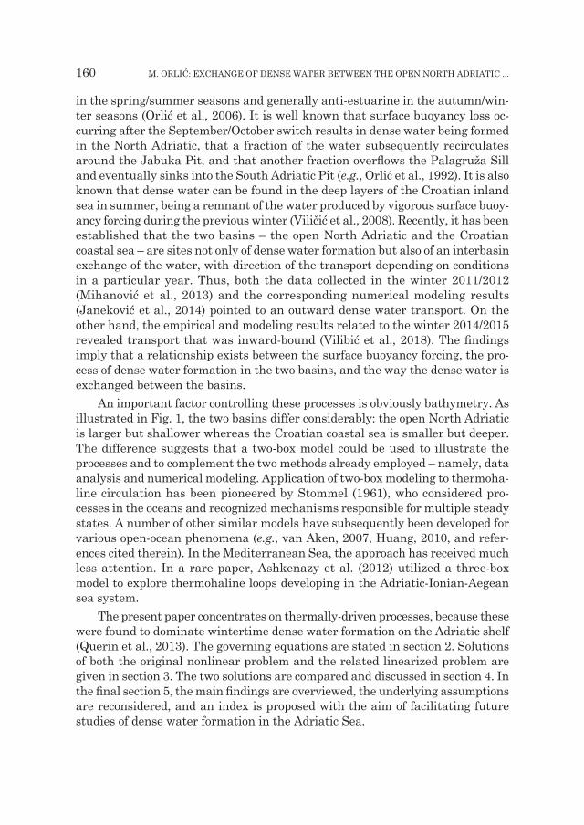
An important factor controlling these processes is obviously bathymetry. As illustrated in Fig. 1, the two basins differ considerably: the open North Adriatic is larger but shallower whereas the Croatian coastal sea is smaller but deeper. The difference suggests that a two-box model could be used to illustrate the processes and to complement the two methods already employed – namely, data analysis and numerical modeling. Application of two-box modeling to thermoha-line circulation has been pioneered by Stommel (1961), who considered pro-cesses in the oceans and recognized mechanisms responsible for multiple steady states. A number of other similar models have subsequently been developed for various open-ocean phenomena (e.g., van Aken, 2007, Huang, 2010, and refer-ences cited therein). In the Mediterranean Sea, the approach has received much less attention. In a rare paper, Ashkenazy et al. (2012) utilized a three-box model to explore thermohaline loops developing in the Adriatic-Ionian-Aegean sea system.

The present paper concentrates on thermally-driven processes, because these were found to dominate wintertime dense water formation on the Adriatic shelf (Querin et al., 2013). The governing equations are stated in section 2. Solutions of both the original nonlinear problem and the related linearized problem are given in section 3. The two solutions are compared and discussed in section 4. In the final section 5, the main findings are overviewed, the underlying assumptions are reconsidered, and an index is proposed with the aim of facilitating future studies of dense water formation in the Adriatic Sea.

GEOFIZIKA, VOL. 35, NO. 2, 2018, 159–175 161

2. Governing equationsThe Adriatic basins are schematized as illustrated in Fig. 2. Subscripts 1

and 2 indicate larger/shallower and smaller/deeper basins, respectively. The basin lengths are denoted by L and their depths by H, whereas widths of the two

Figure 1. Top: Position of three profiles (a, b and c) extending from the Italian to the Croatian coast of the North Adriatic. In the inserted figure, the open North Adriatic is marked on the left and the Croatian coastal sea is indicated on the right. Bottom: Depths along the three profiles. Also shown is the average depth (heavy black line).

162 M. ORLIĆ: EXCHANGE OF DENSE WATER BETWEEN THE OPEN NORTH ADRIATIC ...

basins are presumed to be similar. It is further assumed that the basins lose heat to the atmosphere at constant (and negative) rates Q1 and Q2; this mimics the surface heat loss that is pronounced in the Adriatic from October to February. Moreover, the basins are allowed to exchange heat by advection, which is re-lated to the transport U+ directed from basin 1 to basin 2 and the transport U– directed from basin 2 to basin 1; the former transport may overlay or underlie the latter one and the two compensate each other. Consequently, temperatures T1 and T2 of the two basins are determined by:

C dTdt

QL

T T11

11

2 1= + -( )l (1a)

C dTdt

QL

T T22

22

1 2= + -( )l (1b)

where C1 = ρ0cpH1 and C2 = ρ0cpH2 are the heat capacities, with ρ0 denoting the sea density and cp the specific heat at constant pressure, whereas l is a variable depending on either of the two interbasin transports:

l r r= =+ -0 0c U c Up p

Assuming that the transports depend on the absolute value of the temperature difference between the basins:

U U T T+ -= = -k 1 2

Figure 2. Two boxes schematizing the North Adriatic – its open part (basin 1) and the Croatian coastal waters (basin 2). All the symbols are defined in the text.

GEOFIZIKA, VOL. 35, NO. 2, 2018, 159–175 163

where k is a parameter to be discussed later, in section 4, it is straightforward to show that equations (1) imply:

d T T

dtT T T T Q

CQC

1 21 2 1 2

1

1

2

2

-( )+ - -( ) = -d � (2)

where:

dk=

+( )H L H LH H L L1 1 2 2

1 2 1 2

The solution for the temperature difference could be obtained from (2), sub-ject to the appropriate initial condition. The two temperatures could then be determined from the following equations:

T QCtC L

T T dt K11

1 1 12 1 1

1= + ò -( ) +l (3a)

T QCtC L

T T dt K22

2 2 21 2 2

1= + ò -( ) +l (3b)

which are easy to get from (1). Constants K1 and K2 are defined by the initial conditions [T1(t = 0) = T10, T2(t = 0) = T20].

3. Solutions

3.1. Solution of nonlinear problem

Equation (2) could be written in a slightly different way:

d T T

dtT T T T Q

C1 2

1 2 1 21

11

-( )+ - -( ) = -( )d W (4)

where parameter W is defined as follows:

W = =

QCQC

Q HQ H

2

2

1

1

2 1

1 2� (5)

If it is assumed that the initial temperature difference equals zero (T10 – T20 = 0), the solution of equation (4) depends on parameter W because the sign of the temperature difference is then controlled by the sign of the equation’s right-hand side. In the case W ≤ 1, equation (4) could be transformed to:

d T T

dtT T Q

C2 1

2 12 1

11

-( )+ -( ) = -( )d W � (6a)

164 M. ORLIĆ: EXCHANGE OF DENSE WATER BETWEEN THE OPEN NORTH ADRIATIC ...

whereas in the case W ≥ 1, equation (4) reads:

d T T

dtT T Q

C1 2

1 22 1

11

-( )+ -( ) = -( )d W � (6b)

Both variants (6) are of the type dx/dt + ax2 = b (or dx/dt = b – ax2), with a and b being positive constants, and are therefore reminiscent of an equation often considered by theorists of nonlinear systems (e.g., Drazin, 1992). Explicit solu-tions of equations (6) are possible and, subject to the above stated initial condi-tion, they read:

T TQ

CQC

t2 11

1

1

1

1 11- =

-( ) -( )æ

è

çç

ö

ø

÷÷

£W W

Wd

dtanh ,� � (7a)

T TQ

CQC

t1 21

1

1

1

1 11- =

-( ) -( )æ

è

çç

ö

ø

÷÷

³W W

Wd

dtanh ,� � (7b)

Temperatures in the two basins could be obtained from equations that follow from (3). In the case W ≤ 1 they are:

T Q

CtH L

T T dt K11

1 1 12 1

211= + ò -( ) +

k

T Q

CtH L

T T dt K22

2 2 22 1

221= - ò -( ) +

k

whereas in the case W ≥ 1 they read:

T Q

CtH L

T T dt K11

1 1 11 2

212= - ò -( ) +

k

T QCtH L

T T dt K22

2 2 21 2

222= + ò -( ) +

k

By allowing in the previous equations for (7) and by determining the constants K11, K21, K12 and K22 from the assumed initial conditions (T10 = T20 = T0), it follows for the case W ≤ 1:

TQ C L C LC C L C L

t C LC L C L

QC1

1 1 1 2 2

1 1 1 2 2

2 2

1 1 2 2

1

1

1=

+( )+( )

-+

-( )W W

dtanhh

dQC

t T1

10

1W -( )æ

è

çç

ö

ø

÷÷+ (8a)

TQ C L C LC C L C L

t C LC L C L

QC2

1 1 1 2 2

1 1 1 2 2

1 1

1 1 2 2

1

1

1=

+( )+( )

++

-( )W W

dtanhh

dQC

t T1

10

1W -( )æ

è

çç

ö

ø

÷÷+ (8b)

GEOFIZIKA, VOL. 35, NO. 2, 2018, 159–175 165

and for the case W ≥ 1:

TQ C L C LC C L C L

t C LC L C L

QC1

1 1 1 2 2

1 1 1 2 2

2 2

1 1 2 2

1

1

1=

+( )+( )

++

-( )W W

dtanhh

dQC

t T1

10

1 -( )æ

è

çç

ö

ø

÷÷+

W (8c)

TQ C L C LC C L C L

t C LC L C L

QC2

1 1 1 2 2

1 1 1 2 2

1 1

1 1 2 2

1

1

1=

+( )+( )

-+

-( )W W

dtanhh �

dQC

t T1

10

1 -( )æ

è

çç

ö

ø

÷÷+

W (8d)

With this the nonlinear problem is solved.

3.2. Solution of linearized problemIt is of some interest to consider also an approximate solution of the problem

stated above. The approximation rests on the linearization of the nonlinear term in (4): d eT T T T T T1 2 1 2 1 2- -( ) = -( )with the linear fit being the best if:

- -

-

ò - -( ) - -( )éë ùû -( ) ®T T

T T

max

max

T T T T T T d T T min1 2

1 2

1 2 1 2 1 22

1 2d e

implying that: e d= -

34 1 2T T max

Equation (4) then transforms to:

d T T

dtT T Q

C1 2

1 21

11

-( )+ -( ) = -( )e W (9)

which, subject to the condition according to which the initial temperature differ-ence equals T10 – T20, gives:

T T QC

e T T et t1 2

1

110 201 1- = -( ) -( ) + -( )- -

eW e e (10)

Temperatures in the two basins could then be determined from simplified equations (3):

T Q

CtC L

T T dt K11

1 1 12 1 1= + ò -( ) +

l

T Q

CtC L

T T dt K22

2 2 21 2 2= + ò -( ) +

l

166 M. ORLIĆ: EXCHANGE OF DENSE WATER BETWEEN THE OPEN NORTH ADRIATIC ...

where it has to be taken into account that l = r0cpke/d for the linearized problem. By allowing for (10) and the initial temperatures equaling T10 and T20, it follows:

TQ C L C LC C L C L

t Q C LC C L C L1

1 1 1 2 2

1 1 1 2 2

1 2 2

1 1 1 2 21 1=

+( )+( )

++( )

-( )W

eW --( ) - +

-( ) -( ) +- -e C LC L C L

T T e Tt te e2 2

1 1 2 210 20 101

TQ C L C LC C L C L

t Q C LC C L C L1

1 1 1 2 2

1 1 1 2 2

1 2 2

1 1 1 2 21 1=

+( )+( )

++( )

-( )W

eW --( ) - +

-( ) -( ) +- -e C LC L C L

T T e Tt te e2 2

1 1 2 210 20 101 (11a)

TQ C L C LC C L C L

t Q LC L C L

e21 1 1 2 2

1 1 1 2 2

1 1

1 1 2 21 1=

+( )+( )

-+( )

-( ) - -W

eW ett tC L

C L C LT T e T( ) + +-( ) -( ) +-1 1

1 1 2 210 20 201 e

TQ C L C LC C L C L

t Q LC L C L

e21 1 1 2 2

1 1 1 2 2

1 1

1 1 2 21 1=

+( )+( )

-+( )

-( ) - -W

eW ett tC L

C L C LT T e T( ) + +-( ) -( ) +-1 1

1 1 2 210 20 201 e (11b)

This completes the solution of the linearized problem. In the special case T10 = T20 = T0, this solution could be compared to the previously obtained solution of the nonlinear problem. In that case, it is easy to show that equation (10) and the definition of e imply:

T T

QCmax1 2

1

1

4 13

1- =-( )

£W

dW,�

T TQ

Cmax1 21

1

4 13

1- =-( )

³W

dW, �

which enables the maximum absolute value of the temperature difference to be estimated. The estimation appears to be acceptable also for the non-zero initial temperature difference when the latter is relatively small.

4. Results and discussion

As is always the case with explicit solutions, their main advantage is that it is easy to analyze the dependence of the solutions on the controlling parameters. In the present case, the basin dimensions are estimated at H1 = 40 m, H2 = 80 m, L1 = 150 km and L2 = 50 km so as to roughly correspond to the North Adriatic dimensions. The surface heat fluxes are allowed to extend over a range of values: Q1 between –150 W/m2 and –100 W/m2 (in accordance with the results obtained by Supić and Orlić, 1999) and W from 0.5 to 1.5 (which implies Q2 = WQ1H2/H1 that varies between –450 W/m2 and –100 W/m2). The sea density r0 is assumed

GEOFIZIKA, VOL. 35, NO. 2, 2018, 159–175 167

to equal 103 kg/m3 whereas the specific heat at constant pressure cp is taken as 4×103 J/(kg °C). For the initial conditions, a typical average value for the sum-mertime Adriatic is chosen for both basins (T10 = T20 = T0 = 20 °C) or just for the first basin (T10 = 20 °C) while it is slightly varied for the second basin (T20 = 18 °C and T20 = 22 °C). Finally, special care is needed while selecting k – the param-eter that defines the dependence of the transports on the absolute value of the temperature difference between the two basins. If it is assumed that currents change relatively slowly, over a time interval considerably exceeding the inertial period, it may be expected that the pressure gradient is balanced by the Coriolis acceleration and friction. Consequently, the following is valid:

c c c kg g=+

- ´( )ff r

f r2 2

where c is the current, cg is the geostrophic current, k is the unit vector directed vertically upwards, f is the Coriolis parameter, and r is the coefficient of friction (originally introduced by Guldberg and Mohn, 1876, 1880). The cross-isobar com-ponent of the current then depends on the coefficient of friction: if the coefficient

Figure 3. Temperature difference (T2 – T1) as a function of time, obtained with both the nonlinear and linearized models when the initial difference vanishes. Surface heat flux equals –100 W/m2 above the first basin and –100 W/m2, –200 W/m2 and –300 W/m2 (corresponding to W = 0.5, 1 and 1.5, respectively) above the second basin. All the other parameters are defined in the text.

168 M. ORLIĆ: EXCHANGE OF DENSE WATER BETWEEN THE OPEN NORTH ADRIATIC ...

vanishes, there is no such component; if the coefficient is close to the Coriolis parameter, the component equals |cg|/2 and is directed from the higher pressure towards the lower pressure. In the latter case one gets k close to 0.1 m2/(s °C) when invoking the thermal wind equation, if the depth is of O(102 m), the dis-tance between the two boxes is of O(105 m), the Coriolis parameter equals 10–4 1/s, the coefficient of thermal expansion is 2×10–4 1/°C, and the acceleration due to gravity is approximated at 10 m/s2. Because, however, parameter k is estimated on the basis of a simplified dynamics, a more general discussion would necessi-tate the parameter to be varied to some extent – or even to be obtained through an inversion of the empirical data.

The discussion of the present results will first concentrate on their variabil-ity related to the changes of two parameters (Q1 and W), with the other param-eters having the values given above. Figure 3 shows how the temperature dif-ference (T2 – T1), obtained as a solution of both the nonlinear and linearized problems, evolves from zero, if Q1 = –100 W/m2 and W = 0.5, 1 and 1.5 (correspond-ing to Q2 = –100 W/m2, –200 W/m2 and –300 W/m2, respectively). It is obvious that the solution of the linearized problem closely follows the solution of the nonlinear problem. Moreover, it is evident that both solutions heavily depend on the parameter W: if W < 1, basin 1 is colder than basin 2 and, therefore, the cold, dense water is transported from basin 1 to basin 2; if W = 1, the temperature difference vanishes and no transport develops between the basins; if W > 1, basin 2 is colder than basin 1 and, consequently, the cold, dense water is transported from basin 2 to basin 1. Finally, it is manifest that the temperature difference tends to a maximum or minimum value. The nonlinear model implies the follow-ing extremes:

Figure 4. Extreme value of the temperature difference T2 – T1 (°C) as a function of the surface heat fluxes above the first basin (Q1) and the second basin (Q2, defined by parameter W such that Q2 = WQ1H2/H1 = 2WQ1 for the present selection of H1 = 40 m and H2 = 80 m). The value was obtained with the nonlinear model. Positive value of the difference implies transport of cold, dense water from the first basin to the second basin whereas negative value of the difference indicates transport in the opposite direction.

GEOFIZIKA, VOL. 35, NO. 2, 2018, 159–175 169

Figure 5. Temperatures of the two basins (T1 and T2) as functions of time, obtained with nonlinear model (top) and linearized model (bottom) when the two initial temperatures equal 20 °C. Surface heat flux equals –100 W/m2 above the first basin and –100 W/m2, –200 W/m2 and –300 W/m2 (cor-responding to W = 0.5, 1 and 1.5, respectively) above the second basin. All the other parameters are defined in the text.

T TQ

Cmax2 11

1

11-( ) =

-( )£

W

dW,�

T TQ

Cmin2 11

1

11-( ) = -

-( )³

W

dW,�

and the linearized model gives similar values. For our selection of controlling parameters, the extremes are illustrated in Fig. 4 and it is obvious that they reach ± 3 °C. The transports corresponding to these extremes amount to 0.3 m2/s in both directions.

The solutions enable not only the temperature difference but also the tem-peratures of the two basins (T1 and T2) to be computed. Figure 5 shows the tem-peratures corresponding to the Q1 and W values given above, when the initial

170 M. ORLIĆ: EXCHANGE OF DENSE WATER BETWEEN THE OPEN NORTH ADRIATIC ...

temperatures of the two basins are equal. Again, it is clearly visible that the solu-tions of nonlinear and linearized problems are similar. Both sets of solutions reveal a temporal decrease of the basin temperatures. Moreover, the sign of the tem-perature difference between the two basins depends on the parameter W, as was also observed by considering the difference itself. The fact that the temperature difference tends to a limiting value while the basin temperatures continue to de-crease indicates that the sum of surface heat loss and lateral heat gain in one basin tends to become equal to the sum of surface and lateral heat losses in the other basin. The typical e-folding time t is, according to the nonlinear model:

td W

W=-( )

£C

Q1

1 11,�

td W

W=-( )

³C

Q1

1 11,�

and very similar according to the linearized model. Thus, for example, with Q1 = –100 W/m2, W = 0.5 or W = 1.5, and the other parameters as given above, the time equals 3.4 months.

In order to illustrate a possible effect of temperature-related preconditioning of dense water formation, also shown are the temperature differences (Fig. 6)

Figure 6. Temperature difference (T2 – T1) as a function of time, obtained with the linearized model when the initial temperature of the first basin equals 20 °C and the initial temperature of the second basin is 22 °C (left) or 18 °C (right). Surface heat flux equals –100 W/m2 above the first basin and –100 W/m2, –200 W/m2 and –300 W/m2 (corresponding to W = 0.5, 1 and 1.5, respectively) above the second basin. All the other parameters are defined in the text.

GEOFIZIKA, VOL. 35, NO. 2, 2018, 159–175 171

and the temperatures of the two basins (Fig. 7) obtained as solutions of the lin-earized problem when the initial temperature of the first basin (T10) equals 20 °C and the initial temperature of the second basin (T20) is either 22 °C or 18 °C. The influence of initial conditions is most obvious for the cases for which the tem-perature difference changes sign, within the time interval t0 defined by:

te

eW

eW

0

1

110

20

10

1

1

11 1

1=

-( ) + -æ

èç

ö

ø÷

-( )ln

QC

T TT

QC

Figure 7. Temperatures of the two basins (T1 and T2) as functions of time, obtained with linearized model when the initial temperature of the first basin equals 20 °C and the initial temperature of the second basin is 22 °C (top) or 18 °C (bottom). Surface heat flux equals –100 W/m2 above the first basin and –100 W/m2, –200 W/m2 and –300 W/m2 (corresponding to W = 0.5, 1 and 1.5, respectively) above the second basin. All the other parameters are defined in the text.

172 M. ORLIĆ: EXCHANGE OF DENSE WATER BETWEEN THE OPEN NORTH ADRIATIC ...

For Q1 = –100 W/m2, T20/T10 = 1.1 combined with W = 1.5 or T20/T10 = 0.9 combined with W = 0.5, and the other parameters as given above, the time interval equals 1.9 months. Otherwise, the temperatures and related differences tend to the previously obtained limiting values, more slowly if the initial temperature dif-ferences and the surface heat fluxes are opposed than if they act in the same sense.

5. ConclusionA simple model, allowing for the surface heat loss from two basins and for

an advective exchange of heat between the basins, has been formulated. Ex-plicit solution has been obtained, not only for the original, nonlinear problem but also for a simplified, linearized problem, when the initial temperature difference between the two basins vanishes. Moreover, the effect of initial temperature difference has been explored with the linearized model. The solutions point to a continuous temperature decrease in the two basins, with the rate of decrease depending on the initial temperature difference, surface heat losses and basin dimensions. The solutions also indicate that the sign of the temperature differ-ence between the two basins could be positive or negative, implying that cold, dense water could be transported either way. Additionally, the solutions reveal that there is a tendency for the temperature difference to stabilize while the temperatures themselves decrease, thus suggesting that the combined surface heat loss and advective heat gain in one basin come close to the combined surface and advective heat losses in the other basin.

There are several ways to improve the present model, even while retaining the two-box geometry. One way is to allow for the surface water fluxes and the corresponding salinity changes. In so far as the surface fluxes are kept fixed and the equation of state is assumed to be linear, this would result in equations that are equivalent to the present ones, with the surface heat fluxes and temperatures being substituted by the surface buoyancy fluxes and densities, respectively. The equivalence of the equations means, of course, that the solutions obtained could also be applied to that case. Additionally, the generalized equations would allow salinity-related preconditioning of dense water formation to be allowed for, by imposing non-zero initial difference between salinities and therefore between densities of the two basins in accordance with the recent finding of Mihanović et al. (2018). Another way to improve the present model is to introduce the surface heat flux that depends on the sea temperature. The data provided by Supić and Orlić (1999) suggest that Q1 and Q2 in equations (1) could be substituted by Q1* – nT1 + mdT1/dt and Q2* – nT2 + mdT2/dt, respectively (where Q1* and Q2* are the temperature-independent contributions to the surface heat flux whereas n and m are constants that quantify the temperature dependence of the flux). This could result in some novel findings. On the other hand, the temperature-depen-dent terms appear to be relatively unimportant if the time scale considered is

GEOFIZIKA, VOL. 35, NO. 2, 2018, 159–175 173

small when compared to the reference time scales C1/n and C2/n and if the ratios m/C1 and m/C2 are small. On the basis of available Adriatic data, n is estimated at about 2.5 W/(m2 °C) whereas m is found to be close to 3.3×107 J/(m2 °C). For the basin depths considered here, this implies that the reference time scales amount to 2–4 years and that the above mentioned ratios do not surpass 0.1–0.2.

The present model could be further generalized by addition of the third box so as to allow not only for interaction of the open North Adriatic with the Croa-tian coastal sea but also for their interaction with the South Adriatic and East Mediterranean Seas. In this way it would be possible to consider the influence of replenishment of the open North Adriatic and the Croatian coastal sea on dense water formation. Having in mind, however, that the third box would be much larger than the two boxes already considered, it could be expected that the e-folding time characterizing the Adriatic-Mediterranean system would be much larger than the e-folding time characteristic of the intra-Adriatic system. The large response time has already been observed: Orlić et al. (2006) recorded sur-face inflow to the Adriatic in May 2003 that was related to surface cooling of the Adriatic and relatively warm conditions prevailing in the East Mediterranean in the winter 2002/2003. This strongly suggests that the response of a large system to the forcing is slower than the response of a small system and that the two-box approximation utilized here is reasonable if the time interval considered does not surpass a season or so and if the change of the Adriatic dynamics in September/October is pronounced.

Sensitive dependence of the present solutions on the initial temperatures, surface heat losses and basin dimensions implies that an index could be useful in documenting year-to-year variability of dense water formation in the North Adriatic. While estimating the index under real-world conditions, one has to take into account that initial temperatures vary in space, that surface heat fluxes vary in both space and time and that the depths are not uniform. A possibility would be to define the index P in the following way:

(12)

with the integration being carried out over the sea surface Si, the volume Vi, and the time interval Q. The index combines the ratio of surface heat loss per unit depth between the two basins and the ratio of initial temperatures. Its applica-tion to the Adriatic would benefit from the Croatian coastal sea (i = 2) being relatively well defined by the chain of islands and therefore from an easy deter-mination of the corresponding surface and volume. More care would be needed while determining the surface and volume of the open North Adriatic (i = 1) and particularly its southeast boundary. As for the integration over time, it could be

174 M. ORLIĆ: EXCHANGE OF DENSE WATER BETWEEN THE OPEN NORTH ADRIATIC ...

performed from the beginning of the cooling season (usually October, t = 0) until its culmination (typically February, t = Θ). The index definition (12) could be extended by substituting the surface heat flux and temperature by the surface buoyancy flux and density, respectively, but the surface area over which the river inflows are distributed would need to be carefully considered. Finally, the index could be estimated for a number of years with the aim of checking wheth-er it is a useful indicator of the way the dense water is transported between the open North Adriatic and the Croatian coastal sea, an inward (outward) transport being expected for small (large) values of the index if replenishment of the two basins is of secondary importance.

Acknowledgment – I am indebted to Maja Bubalo and Iva Međugorac for their help with the figures. This work has been fully supported by Croatian Science Foundation under the project HRZZ-IP-2013-2831 (CARE).

References

Ashkenazy, Y., Stone, P. H. and Malanotte-Rizzoli, P. (2012): Box modelling of the Eastern Mediter-ranean Sea, Physica A, 391, 1519–1531, DOI: 10.1016/j.physa.2011.08.026.

Drazin, P. G. (1992): Nonlinear systems. Cambridge University Press, Cambridge, 317 pp.Guldberg, C. M. and Mohn, H. (1876): Études sur les mouvements de l’atmosphère, Première partie.

A. W. Brøgger, Christiania, 39 pp.Guldberg, C. M. and Mohn, H. (1880): Études sur les mouvements de l’atmosphère, Deuxième partie.

A. W. Brøgger, Christiania, 53 pp.Huang, R. X. (2010): Ocean circulation – Wind-driven and thermohaline processes. Cambridge Uni-

versity Press, Cambridge, 791 pp.Janeković, I., Mihanović, H., Vilibić, I. and Tudor, M. (2014): Extreme cooling and dense water for-

mation estimates in open and coastal regions of the Adriatic Sea during the winter of 2012, J. Geophys. Res., 119, 3200–3218, DOI: 10.1002/2014JC009865.

Mihanović, H., Vilibić, I., Carniel, S., Tudor, M., Russo, A., Bergamasco, A., Bubić, N., Ljubešić, Z., Viličić, D., Boldrin, A., Malačič, V., Celio, M., Comici, C. and Raicich, F. (2013): Exceptional dense water formation on the Adriatic shelf in the winter of 2012, Ocean Sci., 9, 561–572, DOI: 10.5194/osd-9-3701-2012.

Mihanović, H., Janeković, I., Vilibić, I., Kovačević, V. and Bensi, M. (2018): Modelling interannual changes in dense water formation on the northern Adriatic shelf, Pure Appl. Geophys., 175, 4065–4081, DOI: 10.1007/s00024-018-1935-5.

Orlić, M., Gačić, M. and LaViolette, P. E. (1992): The currents and circulation of the Adriatic Sea, Oceanol. Acta, 15, 109–124.

Orlić, M., Dadić, V., Grbec, B., Leder, N., Marki, A., Matić, F., Mihanović, H., Beg Paklar, G., Pasarić, M., Pasarić Z. and Vilibić, I. (2006): Wintertime buoyancy forcing, changing seawater properties, and two different circulation systems produced in the Adriatic, J. Geophys. Res., 111, C03S07, 1–21, DOI: 10.1029/2005JC003271.

Querin, S., Cossarini, G. and Solidoro, C. (2013): Simulating the formation and fate of dense water in a midlatitude marginal sea during normal and warm winter conditions, J. Geophys. Res., 118, 885–900, DOI: 10.1002/jgrc.20092.

Stommel, H. (1961): Thermohaline convection with two stable regimes of flow, Tellus, 13, 224–230, DOI: 10.1111/j.2153-3490.1961.tb00079.x.

Supić, N. and Orlić, M. (1999): Seasonal and interannual variability of the northern Adriatic surface fluxes, J. Marine Sys., 20, 205–229, DOI: 10.1016/S0924-7963(98)00083-9.

GEOFIZIKA, VOL. 35, NO. 2, 2018, 159–175 175

van Aken, H.M. (2007): The oceanic thermohaline circulation – An introduction. Springer, New York, 326 pp.

Vilibić, I., Mihanović, H., Janeković, I., Denamiel, C., Poulain, P.M., Orlić, M., Dunić, N., Dadić, V., Pasarić, M., Muslim, S., Gerin, R., Matić, F., Šepić, J., Mauri, E., Kokkini, Z., Tudor, M., Kovač, Ž. and Džoić, T. (2018): Wintertime dynamics in the coastal northeastern Adriatic Sea – The NAdEx 2015 experiment, Ocean Sci., 14, 237–258, DOI: 10.5194/os-14-237-2018.

Viličić, D., Orlić, M. and Jasprica, N. (2008): The deep chlorophyll maximum in the coastal north-eastern Adriatic Sea, July 2007, Acta Bot. Croat., 67, 33–43.

SAŽETAK

Razmjena guste vode između otvorenog Sjevernog Jadrana i hrvatskog obalnog mora: eksplicitno rješavanje nelinearnog problema

Mirko Orlić

Već je neko vrijeme poznato da se gusta voda stvara zimi u Sjevernom Jadranu u dva područja – na otvorenom moru i u hrvatskom obalnom moru. Nedavno je utvrđeno da dolazi i do transporta guste vode između ta dva područja, pri čemu su moguća oba smjera transporta. U ovom je članku razvijen jednostavan model dvije kutije radi interpretacije tih nalaza. Model uvažava gubitak topline s površine dvaju područja te advektivnu razm-jenu topline između područja. Dobivena su eksplicitna rješenja, ne samo za izvorni, nelin-earni problem nego i za pojednostavljeni, linearizirani problem, za slučaj kad iščezava početna razlika temperatura između dva bazena. Osim toga, razmotren je i utjecaj početne razlike temperatura pomoću lineariziranog modela. Rješenja ukazuju na kontinuirano smanjenje temperature u dva područja, pri čemu razlika temperatura teži graničnoj vri-jednosti. Takva je vremenska promjenjivost određena početnom razlikom temperatura, površinskim protocima topline i dimenzijama bazena te sugerira da se suma površinskog gubitka topline i advektivnog primitka topline u jednom bazenu s vremenom približava sumi površinskog i advektivnog gubitka topline u drugom bazenu. Rješenja također po-kazuju da predznak temperaturne razlike između dva bazena može biti pozitivan ili negativan, što znači da hladna, gusta voda može biti transportirana u oba smjera. Napo-sljetku, predložen je indeks koji uključuje početne temperature, površinske protoke topline i dubine bazena i koji bi trebao omogućiti da se kvantificira relativna važnost dvaju sjevernojadranskih područja stvaranja guste vode za svaku pojedinu zimu.

Ključne riječi: stvaranje guste vode, advekcija, model dvije kutije, Sjeverni Jadran

Corresponding author’s address: Mirko Orlić, Andrija Mohorovičić Geophysical Institute, Department of Geophys-ics, Faculty of Science, University of Zagreb, Horvatovac 95, HR-10000 Zagreb, Croatia; tel: +385 1 4605 930; e-mail: morlic@gfz.hr

This work is licensed under a Creative Commons Attribution-NonCommercial 4.0 Interna-

tional License.