Exchange Economiesand Networks

Networked LifeCSE 112

Spring 2005Prof. Michael Kearns

Market Economies• Suppose there are a bunch of different goods

– wheat, rice, paper, raccoon pelts, matches, grain alcohol,…– no differences or distinctions within a good: rice is rice

• We may all have different initial amounts or endowments– I might have 10 sacks of rice and two raccoon pelts– you might have 6 bushels of wheat, 2 boxes of matches– etc. etc. etc.

• Of course, we may want to exchange some of our goods– I can’t eat 10 sacks of rice, and I need matches to light a fire– it’s getting cold and you need raccoon mittens– etc. etc. etc.

• How should we engage in exchange?• What should be the rates of exchange?• These are among the oldest questions in economics

Cash and Prices• Suppose we introduce an abstract good called cash

– no inherent value– simply meant to facilitate trade, encode exchange rates

• And now suppose we introduce prices in cash– i.e. rates of exchange between each “real” good and

cash

• Then if we all believed in cash and the prices…– we might try to sell our initial endowments for cash– then use the cash to buy exactly what we most want

• But will there really be:– others who want to buy all of our endowments? (demand)– others who will be selling what we want? (supply)

Mathematical Economics• Have k abstract goods or commodities g1, g2, … , gk• Have n consumers or players• Each player has an initial endowment e = (e1,e2,…,ek)

> 0• Each consumer has their own utility function:

– assigns a personal valuation or utility to any amounts of the k goods

– e.g. if k = 4, U(x1,x2,x3,x4) = 0.2*x1 + 0.7*x2 + 0.3*x3 + 0.5*x4

– here g2 is my “favorite” good --- but it might be expensive– generally assume utility functions are insatiable

• always some bundle of goods you’d prefer more

– utility functions not necessarily linear, though

Market Equilibrium• Suppose we post prices p = (p1,p2,…,pk) for the k goods• Assume consumers are rational:

– they will attempt to sell their endowment e at the prices p (supply)– if successful, they will get cash e*p = e1*p1 + e2*p2 + … + ek*pk– with this cash, they will then attempt to purchase x = (x1,x2,…,xk)

that maximizes their utility U(x) subject to their budget (demand)– example:

• U(x1,x2,x3,x4) = 0.2*x1 + 0.7*x2 + 0.3*x3 + 0.5*x4• p = (1.0,0.35,0.15,2.0)• look at “bang for the buck” for each good i, wi/pi:

– g1: 0.2/1.0 = 0.2; g2: 0.7/0.35 = 2.0; g3: 0.3/0.15 = 2.0; g4: 0.5/2.0 = 0.25– so we will purchase as much of g2 and/or g3 as we can subject to budget

• Say that the prices p are an equilibrium if there are exactly enough goods to accomplish all supply and demand steps

• That is, supply exactly balances demand --- market clears

The Phone Call from Stockholm• Arrow and Debreu, 1954:

– There is always a set of equilibrium prices!– Both won Nobel prizes in Economics

• Intuition: suppose p is not an equilibrium– if there is excess demand for some good at p, raise its price– if there is excess supply for some good at p, lower its price– the “invisible hand” of the market

• The trickiness:– changing prices can radically alter consumer preferences

• not necessarily a gradual process; see “bang for the buck” argument

– everyone reacting/adjusting simultaneously– utility functions may be extremely complex

• May also have to specify “consumption plans”:– who buys exactly what from whom– example:

• A has Fruit Loops and Lucky Charms, but wants granola• B and C have only granola, both want either FL or LC (indifferent)• need to “coordinate” B and C to buy A’s FL and LC

Remarks• A&D 1954 a mathematical tour-de-force

– resolved and clarified a hundred of years of confusion– proof related to Nash’s; (n+1)-player game with “price player”

• Actual markets have been around for millennia– highly structured social systems– it’s the mathematical formalism and understanding that’s new

• Model abstracts away details of price adjustment process– modern financial markets– pre-currency bartering and trade– auctions– etc. etc. etc.

• Model can be augmented in various way:– labor as a commodity– firms producing goods from raw materials and labor– etc. etc. etc.

• “Efficient markets” ~ in equilibrium (at least at any given moment)

Network Economics• All of what we’ve said so far assumes:

– that anyone can trade (buy or sell) with anyone else– wheat bought from Nikhil is the same as wheat bought from Elliot– equivalently, exchange takes place on a complete network– global prices must emerge due to competition

• But there are many economic settings in which everyone is not free to trade with everyone else– geography:

• perishability: you buy groceries from local markets so it won’t spoil• labor: you purchases services from local residents

– legality:• if one were to purchase drugs, it is likely to be from an acquaintance (no

centralized market possible)• peer-to-peer music exchange

– politics:• there may be trade embargoes between nations

– regulations:• on Wall Street, certain transactions (within a firm) may be prohibited

A Network Model of Market Economies

• Still begin with the same framework:– k goods or commodities– n consumers, each with their own endowments and utility functions

• But now assume an undirected network dictating exchange– each vertex is a consumer– edge between i and j means they are free to engage in trade– no edge between i and j: direct exchange is forbidden

• Note: can “encode” network in goods and utilities– for each raw good g and consumer i, introduce virtual good (g,i)– think of (g,i) as “good g when sold by consumer i”– consumer j will have

• zero utility for (g,i) if no edge between i and j• j’s original utility for g if there is an edge between i and j

Network Equilibrium

• Now prices are for each (g,i), not for just raw goods– permits the possibility of variation in price for raw goods– prices of (g,i) and (g,j) may differ– what would cause such variation at equilibrium?

• Each consumer must still behave rationally– attempt to sell all of initial endowment, but only to NW

neighbors– attempt to purchase goods maximizing utility within budget– will only purchase g from those neighbors with minimum price

for g

• Market equilibrium still always exists!– set of prices (and consumptions plans) such that:

• all initial endowments sold (no excess supply)• no consumer has money left over (no excess demand)

A Preferential Attachment Modelfor Buyer-Seller Networks

• Probabilistically generates a bipartite graph• Buyers and sellers added in pairs at each time step

– buyers: start with 1 unit of cash, have utility only for wheat– sellers: start with 1 unit of wheat, have utility only for cash

• All edges between buyers and sellers• Each new party will have links back to extant graph

– note: generates bipartite trees – larger generates cyclical graphs

• Distribution of new buyer’s links:– with prob. 1 – : extant seller chosen w.r.t. preferential

attachment– with prob. : extant seller chosen uniformly at random– is pure pref. att.; is “like” Erdos-Renyi model

• So () characterizes distribution of generative model

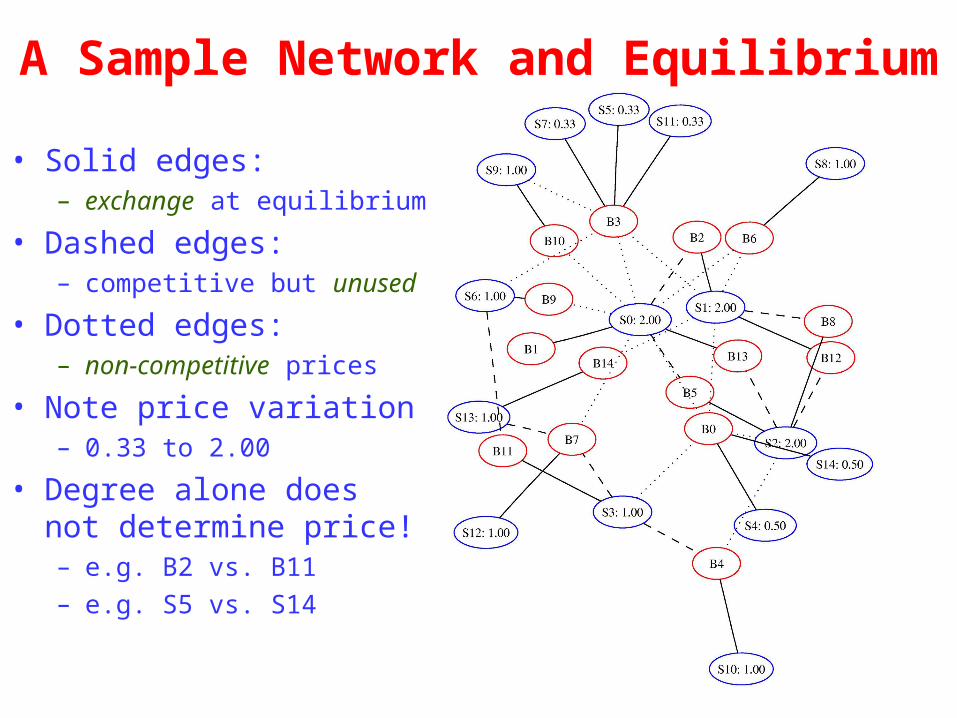
A Sample Network and Equilibrium

• Solid edges:– exchange at equilibrium

• Dashed edges:– competitive but unused

• Dotted edges:– non-competitive prices

• Note price variation– 0.33 to 2.00

• Degree alone does not determine price!– e.g. B2 vs. B11– e.g. S5 vs. S14

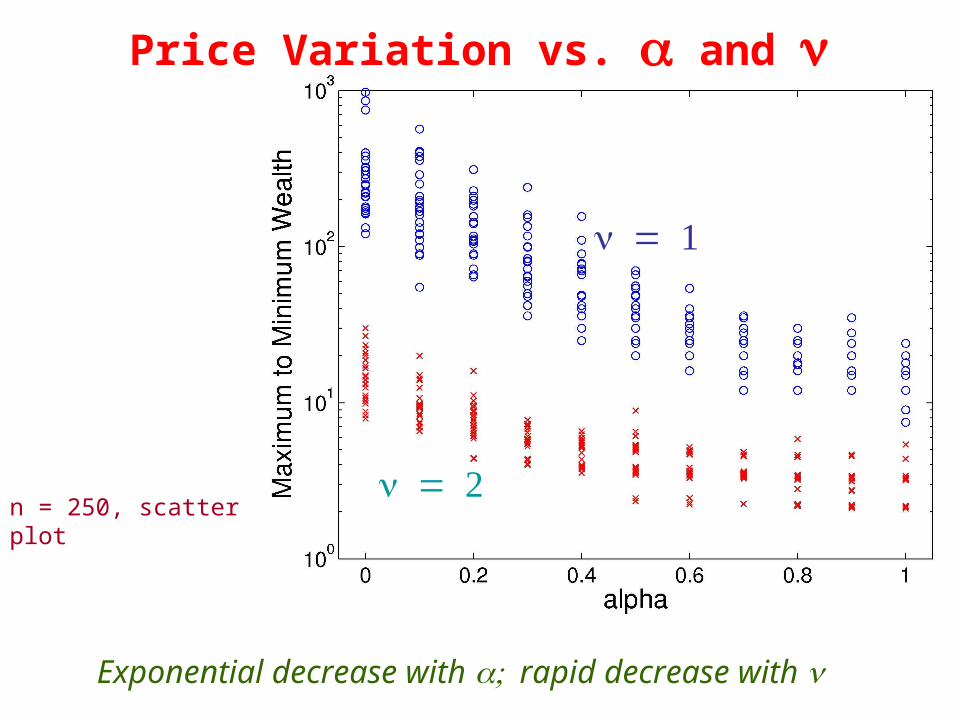
Price Variation vs. and

n = 250, scatter plot

Exponential decrease with rapid decrease with

(Statistical) Structure and Outcome

• Wealth distribution at equilibrium:– Power law (heavy-tailed) in networks generated by preferential attachment – Sharply peaked (Poisson) in random graphs

• Price variation (max/min) at equilibrium: – Grows as a root of n in preferential attachment– None in random graphs

• Random graphs result in “socialist” outcomes– Despite lack of centralized formation process

• Price variation in arbitrary networks:– Characterized by an expansion property– Connections to eigenvalues of adjacency matrix– Theory of random walks– Economic vs. geographic isolation

U.N. Comtrade Data Network

USA: 4.42Germany: 4.01Italy: 3.67France: 3.16Japan: 2.27

Full Network

sorted equilibrium prices

vertex degree

pri

ce

European Union Network

USA: 4.42Germany: 4.01Italy: 3.67France: 3.16Japan: 2.27

Full Network EU network

sorted equilibrium prices

vertex degree

pri

ce

EU: 7.18USA: 4.50Japan: 2.96

Network Exchange Experiments:

Tuesday, April 12• Participation mandatory• Each of you will be assigned a role as either a “buyer” or “seller”• Will play two rounds of 25 minutes each• Endowments: In each round, you will be issued either

– 10 units of cash (buyers)– 10 units of wheat (sellers)

• Write your name on each unit of your endowment• In the first round, you are permitted to trade only with your Lifester neighbors

– so at the end, you should hold only units from your initial endowments or from your neighbors

• In the second round, you are permitted to trade with anyone in the class• Utilities: Your score for each round is the number of units you hold of the other good

– buyer’s score = number of units of wheat held– seller’s score = number of units of cash held

• At the end of each round, turn in an envelope with your name & containing your holdings

• Cash (real) prizes:– $25 to party accumulating greatest wealth (amount of other good) in two rounds– $25 to party outperforming equilibrium predictions by the greatest amount– split in case of ties