excel for chemists a comprehensive guide - 2nd edition
TRANSCRIPT

Excel@ for Chemists
Second Edition
Excel for Chemists: A Comprehensive Guide. E. Joseph BilloCopyright 2001 by John Wiley & Sons, Inc.
ISBNs: 0-471-39462-9 (Paperback); 0-471-22058-2 (Electronic)

ExcePfor Chemists A Comprehensive Guide
Second Edition
E. Joseph Billo Department of Chemistry
Boston College Chestnut Hill, Massachusetts
8 WILEY-VCH New York l Chichester l Weinheim l Brisbane l Singapore l Toronto
Excel for Chemists: A Comprehensive Guide. E. Joseph BilloCopyright 2001 by John Wiley & Sons, Inc.
ISBNs: 0-471-39462-9 (Paperback); 0-471-22058-2 (Electronic)

Copyright 2001 by John Wiley and Sons, Inc., New York. All rightsreserved.
No part of this publication may be reproduced, stored in a retrieval systemor transmitted in any form or by any means, electronic or mechanical,including uploading, downloading, printing, decompiling, recording orotherwise, except as permitted under Sections 107 or 108 of the 1976United States Copyright Act, without the prior written permission of thePublisher. Requests to the Publisher for permission should be addressed tothe Permissions Department, John Wiley & Sons, Inc., 605 Third Avenue,New York, NY 10158-0012, (212) 850-6011, fax (212) 850-6008, E-Mail:[email protected].
This publication is designed to provide accurate and authoritativeinformation in regard to the subject matter covered. It is sold with theunderstanding that the publisher is not engaged in rendering professionalservices. If professional advice or other expert assistance is required, theservices of a competent professional person should be sought.
ISBN 0-471-22058-2.
This title is also available in print as ISBN 0-471-39462-9.
For more information about Wiley products, visit our web site atwww.Wiley.com.

SUMMARY OF CONTENTS
PART I Chapter 1 Chapter 2
PART II Chapter 3 Chanter 4 Chapter 5 Chapter 6 Chapter 7 Chapter 8
PART III Chapter 9 Chapter 10 Chapter 11 Chapter 12
PART IV Chapter 13 Chapter 14 Chapter 15 Chapter 16 Chapter 17 Chapter 18 Chapter 19
PART V Chapter 20 Chapter 21 Chapter 22 Chapter 23
PART VI Appendix A Appendix B Appendix C Appendix D Appendix E Appendix F Appendix G
Preface . . . . . . . . . . . . . . . . . . . . . . . . . . . . . . . . . . . . . . . . . . . . . . . . . . . . . . . . . . . . . . . . . . . . . . . ..~...... xix Preface to the First Edition .................................................... xxi Before You Begin
... ............................................................... xx111
THE BASICS Working with Excel ................................................................ 3 Creating Charts: An Introduction ........................................... 47
ADVANCED SPREADSHEET TOPICS Creating Advanced Worksheet Formulas ............................... 59 Creating Array Formulas ...................................................... 91 Advanced Charting Techniques ............................................ 109 Using Excel’s Database Features ........................................... 133 Importing Data into Excel ..................................................... 147 Adding Controls to a Spreadsheet ........................................ 159
SPREADSHEET MATHEMATICS Some Mathematical Tools For Spreadsheet Calculations ....... .169 Graphical and Numerical Methods of Analysis .................... ..19 3 Linear Regression ................................................................ 207 Non-Linear Regression Using the Solver ............................... 223
EXCEL VISUAL BASIC MACROS Visual Basic for Applications: An Introduction ..................... .241 Programming with VBA ....................................................... 251 Working with Arrays in VBA ............................................... 279 Creating Command Macros .................................................. 291 Creating Custom Functions .................................................. 299 Creating Custom Menus and Menu Bars ............................... 309 Creating Custom Toolbuttons and Toolbars ........................... 317
SOME APPLICATIONS Analysis of Solution Equilibria ............................................. 329 Analysis of Spectrophotometric Data .................................... 339 Calculation of Binding Constants .......................................... 349 Analysis of Kinetics Data ...................................................... 373
APPENDICES Selected Worksheet Functions by Category ............................ 391 Alphabet ical List of Selected Worksheet Functions. ............... .397 Selected Visual Basic Keywords by Category ........................ .417 Alphabe tical List of Selected Visual Basic Keywords ............. ,421 Shortcut Keys for PC and Macintosh ..................................... 441 Selected Shortcut Keys by Category ...................................... 457 About the CD-ROM That Accompanies This Book ................ .463
INDEX ................................................................................ 469
V

CONTENTS
Preface . . . . . . . . . . . . . . . . . . . . . . . . . . . . . . . . . . . . . . . . . . . . . . . . . . . . . . . . . . . . . . . . . . . . . . . . . . . . . . . . . . . . . . . . . . . . . . . . . . . . . . . . xix Preface to the First Edition . . . . . . . . . . . . . . . . . . . . . . . . . . . . . . . . . . . . . . . . . . . . . . . . . . . . . . . . . . . . . . . . . . . . . . . . . . . . xxi Before You Begin
. . . . . . . . . . . . . . . . . . . . . . . . . . . . . . . . . . . . . . . . . . . . . . . . . . . . . . . . . . . . . . . . . . . . . . . . . . . . . . . . . . . . . . . . . . xx111
PARTI: THE BASICS 1
Chapter 1 Working with Excel ..................................................................... 3 The Excel Document Window ......................................................................... 3
Changing What Excel Displays .................................................................. 4 Moving or Re-Sizing Documents (Windows) . . . . . . . . . . . . . . . . . . . . . . . . . . . . . . . . . . . . . . . . . . . . . . 5 Moving or Re-Sizing Documents (Macintosh) ............................................. 5
Navigating Around the Workbook .................................................................. 5 Selecting Multiple Worksheets ................................................................... 6 Changing Worksheet Names ..................................................................... 6 Rearranging the Order of Sheets in a Workbook ......................................... 6
Navigating Around the Worksheet .................................................................. 7 Selecting a Range of Cells on the Worksheet .............................................. 7 Selecting Non-Adjacent Ranges ................................................................. 8 Selecting a Block of Cells ........................................................................... 8
Entering Data in a Worksheet ......................................................................... 9 Entering Numbers .................................................................................. 10 How Excel Stores and Displays Numbers ................................................. 10 Entering Text .......................................................................................... 11 Entering Formulas .................................................................................. 11 Adding a Text Box .................................................................................. 12 Entering a Cell Comment ........................................................................ 12 Editing Cell Entries ................................................................................. 13
Excel’s Menus: An Overview ......................................................................... 13 Shortcut Menus ...................................................................................... 15 Menu Commands or Toolbuttons? ............................................................ 15
Opening, Closing and Saving Documents ....................................................... 15 Opening or Creating Workbooks ............................................................. 15 Using Move, Copy or DeleteSheet .......................................................... 16 Using Close or Exit/Quit ....................................................................... 16 Using Save or Save As ........................................................................... 16 The Types of Excel Document ................................................................. 17 Using Save Workspace ........................................................................... 17
Printing Documents ...................................................................................... 18
vii
Excel for Chemists: A Comprehensive Guide. E. Joseph BilloCopyright 2001 by John Wiley & Sons, Inc.
ISBNs: 0-471-39462-9 (Paperback); 0-471-22058-2 (Electronic)

Excel for Chemists
Using Page Setup .................................................................................. 18 Using Print Preview . .............................................................................. 19 Using Print ............................................................................................ 19 Printing a Selected Range of Cells in a Worksheet ..................................... 20 Printing Row or Column Headings for a Multi-Page Worksheet ................ 21
Editing a Worksheet ..................................................................................... 21 Inserting or Deleting Rows or Columns .................................................... 21 Using Cut, Copy and Paste ..................................................................... 22 Using Paste Special ................................................................................ 22 Using Paste Special to Transpose Rows and Columns .............................. 23 Using Clear ............................................................................................ 24 Using Insert .......................................................................................... 24 To Copy, Cut or Paste Using Drag-and-Drop Editing ............................... 24 Duplicating Values or Formulas in a Range of Cells .................................. 25 Absolute, Relative and Mixed References ................................................ 26 Relative References When Using Copy and Cut ........................................ 27 Using AutoFill to Fill Down or Fill Right ................................................ 27 Using AutoFill to Create a Series .............................................................. 28
Formatting Worksheets ................................................................................. 29 Using Column Width and Row Height . . . . . . . . . . . . . . . . . . . . . . . . . . . . . . . . . . . . . . . . . . . . . . . . . . . . 29 Using Alignment ................................................................................... 30 Using Font ............................................................................................. 31 The Alternate Character Set ..................................................................... 32 Entering Subscripts and Superscripts ....................................................... 33 Using Border and Patterns ...................................................................... 33 Using the Format Painter Toolbutton ....................................................... 34
Number Formatting ...................................................................................... 35 Using Excel’s Built-in Number Formats . . . . . . . . . . . . . . . . . . . . . . . . . . . . . . . . . . . . . . . . . . . . . . . . . . . . 35 Custom Number Formats . . . . . . . . . . . . . . . . . . . . . . . . . . . . . . . . . . . . . . . . . . . . . . . . . . . . . . . . . . . . . . . . . . . . . . . . 36 Variable Number Formats . . . . . . . . . . . . . . . . . . . . . . . . . . . . . . . . . . . . . . . . . . . . . . . . . . . . . . . . . . . . . . . . . . . . . . 38 Conditional Number Formats . . . . . . . . . . . . . . . . . . . . . . . . . . . . . . . . . . . . . . . . . . . . . . . . . . . . . . . . . . . . . . . . . . 38 Using the Number Formatting Toolbuttons .............................................. 39 Formatting Numbers Using “Precision as Displayed” ................................ 39
Protecting Data in Worksheets ....................................................................... 40 Using Protection .................................................................................... 40 Protecting a Workbook by Making it Read-Only ....................................... 40
Controlling the Way Documents Are Displayed .............................................. 41 Viewing Several Worksheets at the Same Time ......................................... 41 Using New Window and Arrange .......................................................... 41 Different Views of the Same Worksheet ................................................... 42 Using New Window ............................................................................... 43 Using Split . . . . . . . . . . . . . . . . . . . . . . . . . . . . . . . . . . . . . . . . . . . . . . . . . . . . . . . . . . . . . . . . . . . . . . . . . . . . . . . . . . . . . . . . . . . . . 43 Using Freeze panes ................................................................................ 44
Copying from Excel to Microsoft Word .......................................................... 44 Using Copy and Paste ............................................................................. 45

Contents ix
Making a “Screen Shot” (Macintosh) ......................................................... 45 Making a “Screen Shot” (Windows) .......................................................... 46
Useful References ......................................................................................... 46
Chapter 2 Creating Charts: An Introduction .............................................. 47 Only One Chart Type Is Useful for Chemists .................................................. 47 Creating a Chart ........................................................................................... 47
Creating a Chart Using the ChartWizard .................................................. 47 Activating, Resizing and Moving an Embedded Chart .............................. 50
Formatting Charts: An Introduction ............................................................... 50 Using the Chart Menu ............................................................................. 50 Using Chart Type ... to Switch From One Chart Type to Another ................ 51 Using Chart Options ... to Add Titles, Gridlines or a Legend ...................... 51 Using Location ... to Move or Copy an Embedded Chart ........................... 51
Formatting the Elements of a Chart ................................................................ 51 Selecting Chart Elements ......................................................................... 52 Formatting Chart Elements ...................................................................... 52
PART II: ADVANCED SPREADSHEET TOPICS . . . . . . . . . . . . . . . . . . . . . . . . . . . . . . . . . . . . . . . . . 57
Chapter 3 Creating Advanced Worksheet Formulas .................................... 59 The Elements of a Worksheet Formula ........................................................... 59
Operators ............................................................................................... 59 Absolute, Relative and Mixed References ................................................. 60 Creating and Using 3-D References .......................................................... 60 Creating and Using External References ................................................... 61 Creating an External Reference by Selecting ............................................. 62 Creating an External Reference by Using Paste Link .................................. 62 The External Reference Contains the Complete Directory Path ................... 62 Updating References and Re-Establishing Links ....................................... 62
Entering Worksheet Formulas ....................................................................... 63 Using Names Instead of References ................................................................ 64
Using Define Name ................................................................................ 64 Using Create Names ............................................................................... 65 Using the Drop-Down Name List Box ...................................................... 67 Entering a Name in a Formula by Selecting .............................................. 67
Using Apply Names ............................................................................... 68
Using Paste Name .................................................................................. 68
Deleting Names ...................................................................................... 68
Changing a Name ................................................................................... 69 Names Can Be Local or Global ................................................................. 69
The Label ... Command ............................................................................ 70
Excel Will Create Labels Automatically .................................................... 71
Worksheet Functions: An Overview ............................................................... 71
Function Arguments ............................................................................... 72

X Excel for Chemists
Math and Trig Functions ............................................................................... 72 Functions for Working with Matrices ....................................................... 73
Statistical Functions ...................................................................................... 73 Logical Functions ......................................................................................... 73
The IF Function ....................................................................................... 73 Nested IF Functions ................................................................................ 74 AND, OR and NOT .................................................................................... 76
Date and Time Functions ............................................................................... 76 Date and Time Arithmetic ....................................................................... 78
Text Functions .............................................................................................. 78 The LEN, LEFT, RIGHT and MID Functions .................................................. 78 The UPPER, LOWER and PROPER Functions ................................................ 79 The FIND, SEARCH, REPLACE, SUBSTITUTE and EXACT Functions.. ............ .79 The FIXED and TEXT Functions ................................................................ 80 The VALUE Function ................................................................................ 81 The CODE and CHAR Functions ................................................................. 81
Lookup and Reference Functions ................................................................... 81 The VLOOKUP and HLOOKUP Functions ..................................................... 82 The LOOKUP Function .............................................................................. 82 The INDEX and MATCH Functions ............................................................. 82 Using Wildcard Characters with MATCH, VLOOKUP or HLOOKUP ................ 83 The OFFSET Function .............................................................................. 83
Using Insert Function .................................................................................... 83 A Shortcut to a Function .......................................................................... 85
Creating “Megaformulas” .............................................................................. 85 Troubleshooting the Worksheet ..................................................................... 87
Error Values and Their Meanings ............................................................ 87 Examining Formulas ............................................................................... 87 Finding Dependent and Precedent Cells ................................................... 88 Using Paste List ...................................................................................... 88
Useful References ......................................................................................... 89
Chapter 4 Creating Array Formulas ............................................................ 91 Using Array Formulas .................................................................................. 91
Array Constants . . . . . . . . . . . . . . . . . . . . . . . . . . . . . . . . . . . . . . . . . . . . . . . . . . . . . . . . . . . . . . . . . . . . . . . . . . . . . . . . . . . . . 93 Editing or Deleting Arrays ...................................................................... 94 Formulas That Return an Array Result ..................................................... 94 Creating a Three-Dimensional Array on a Single Worksheet ...................... 95
Evaluating Polynomials or Power Series Using Array Formulas ...................... .96 Using the ROW Function in Array Formulas .............................................. 97 Using the INDIRECT Function in Array Formulas ....................................... 97
Using Array Formulas to Work With Lists ...................................................... 97 Counting Entries in a List Using Multiple Criteria ..................................... 98

Contents xi
Counting Common Entries in Two Lists ................................................... 99 Counting Duplicate Entries in a List ........................................................ 100 Counting Unique Entries in a List ........................................................... 101 Indicating Duplicate Entries in a List ....................................................... 101 Returning an Array of Unique Entries in a List ........................................ 103
Using an Array Formula to Sort a 1-D List ..................................................... 104 Using an Array Formula to Sort a 2-D List ..................................................... 105
Chapter 5 Advanced Charting Techniques ................................................ 109 Good Charts vs. Bad Charts .......................................................................... 109 Charts with More Than One Data Series ........................................................ 110
Plotting Two Different Sets of Y Values in the Same Chart ...................... .llO Plotting Two Different Sets of X and Y Values in the Same Chart.. ........... .lll Another Way to Plot Two Different Sets of X and Y Values.. .................... .112
Extending a Data Series or Adding a New Series ............................................ 114 The Copy and Paste Method ................................................................... 114 The Drag and Drop Method ................................................................... 114 The Color-Coded Ranges Method ........................................................... 114 Using Source Data ... in the Chart Menu .................................................. 116 Editing the SERIES Function in the Formula Bar ....................................... 116
Customizing Charts ..................................................................................... 116 Plotting Experimental Data Points and a Calculated Curve ...................... .116 Adding Error Bars to an XY Chart ........................................................... 118 Adding Data Labels to an XY Chart ........................................................ 120 Charts Suitable for Publication ............................................................... 121
Changing the Default Chart Format .............................................................. 121 Logarithmic Charts ...................................................................................... 122 3-D Charts ................................................................................................... 123
Using Excel’s Built-in 3-D Chart Format .................................................. 123 Charts with Secondary Axes ......................................................................... 124 Getting Creative with Charts ........................................................................ 126
A Chart with an Additional Axis ............................................................ 127 A Chart with an Inset ............................................................................. 129
Linking Chart Text Elements to a Worksheet ................................................. 130 To Switch Plotting Order in an XY Chart ....................................................... 131 Some Chart Specifications (Excel 2000) .......................................................... 132
Chapter 6 Using Excel’s Database Features ................................................ 133 The Structure of a List or Database ................................................................ 133 Sorting a List ............................................................................................... 133
Sorting According to More Than One Field ............................................. 135 Sort Options .......................................................................................... 135
Using AutoFilter to Obtain a Subset of a List ................................................. 136 Using Multiple Data Filters .................................................................... 138
Defining and Using a Database ..................................................................... 138

Xii Excel for Chemists
Creating a Database ............................................................................... 138 Defining a Database ............................................................................... 139 Adding or Deleting Records or Fields ..................................................... 139 Updating a Database Using Data Form ................................................... 139 Finding Records That Meet Criteria ........................................................ 141 Defining and Using Selection Criteria ...................................................... 141 Using Multiple Criteria .......................................................................... 142 Special Criteria for Text Entries ............................................................... 143 Extracting Records ................................................................................. 144
Using Database Functions ............................................................................ 145
Chapter 7 Getting Data into Excel ............................................................. 147 Direct Input of Instrument Data into Excel .................................................... 147 Transferring Files from Other Applications to Excel ...................................... 147
Using the Text Import Wizard ................................................................ 147 Using Text to Columns ........................................................................... 151
From Hard Copy (Paper) to Excel ................................................................. 151 Using a Scanner to Transfer Numeric Data to Excel .................................. 151 Using a Scanner to Transfer Graphical Data to Excel ................................ 154
Selecting Every Nth Data Point ..................................................................... 154 Using AutoFill ....................................................................................... 154 Using the Sampling Tool ........................................................................ 155 Using a Worksheet Formula ................................................................... 157
Chapter 8 Adding Controls to a Spreadsheet ............................................ 159 You Can Add Option Buttons, Check Boxes, List Boxes and Other Controls to a Worksheet ............................................................... 159 How to Add a Control to a Worksheet .......................................................... 160
Control Properties ................................................................................. 161 A List Box on a Worksheet ........................................................................... 163 A Drop-down List Box on a Worksheet ......................................................... 163 Option Buttons and a Drop-down List Box .................................................... 165
PART III: SPREADSHEET MATHEMATICS . . . . . . . . . . . . . . . . . . . . . . . . . . . . . . . . . . . . . . . . . . . . . . 167
Chapter 9 Some Mathematical Tools for Spreadsheet Calculations .......... ..16 9 Looking Up Values in Tables ........................................................................ 169
Getting Values from a One-Way Table .................................................... 169 Getting Values from a Two-Way Table .................................................... 170
Interpolation Methods: Linear ...................................................................... 171 Table Lookup with Linear Interpolation .................................................. 171
Interpolation Methods: Cubic ....................................................................... 173 Numerical Differentiation ............................................................................ 175
First and Second Derivatives of a Data Set ............................................... 175 Derivatives of a Function ........................................................................ 178
Numerical Integration .................................................................................. 179

Contents
An Example: Finding the Area Under a Curve ......................................... 180 Differential Equations .................................................................................. 182
Euler’s Method ...................................................................................... 183 The Runge-Kutta Methods ..................................................................... 184
Arrays, Matrices and Determinants ............................................................... 186 An Introduction to Matrix Algebra .......................................................... 187
Polar to Cartesian Coordinates ..................................................................... 189 Useful Reference .......................................................................................... 191
Chapter 10 Graphical and Numerical Methods of Analysis.. ...................... .193 Finding Roots of Equations ........................................................................... 193
The Graphical Method ........................................................................... 193 The Method of Successive Approximations . . . . . . . . . . . . . . . . . . . . . . . . . . . . . . . . . . . . . . . . . . . . . 194 The Newton-Raphson Method ................................................................ 196
Solving a Problem Using Goal Seek ............................................................... 198 Solving a Problem by Intentional Circular Reference ...................................... 201 Solving Sets of Simultaneous Linear Equations .............................................. 203
Cramer’s Rule ........................................................................................ 204 Solution Using Matrix Inversion ............................................................. 205
Chapter 11 Linear Regression .................................................................... 207 Least-Squares Curve Fitting .......................................................................... 207
Least-Squares Fit to a Straight Line ......................................................... 208 The SLOPE, INTERCEPT and RSQ Functions .............................................. 208 Linear Regression Using LINEST ............................................................. 209 Least-Squares Fit of y = mx + b ............................................................... 211 Regression Line Without an Intercept ...................................................... 211 Weighted Least Squares ......................................................................... 212
Multiple Linear Regression ........................................................................... 212 Linear Regression Using a Power Series .................................................. 214 Linear Regression Using Trendline ......................................................... 214 Linear Regression Using the Analysis ToolPak ........................................ 216
Using the Regression Statistics ...................................................................... 218 Testing Whether an Intercept Is Significantly Different from Zero ............ .218 Testing Whether Two Slopes Are Significantly Different .......................... 219 Testing Whether a Regression Coefficient Is Significant . . . . . . . . . . . . . . . . . . . . . . . . . . . . 220 Testing Whether Regression Coefficients Are Correlated .......................... 220 Confidence Intervals for Slope and Intercept ........................................... 221 Confidence Limits and Prediction Limits for a Straight Line .................... .221
Useful References ........................................................................................ 222
Chapter 12 Non-Linear Regression Using the Solver .*~****...~.~.....*.....*.**~~.,~. 223 Non-Linear Functions *~*..***~*...~~*..*~**.*.,..*~....~..**~~~***....*.~*......~~**.***~...,*‘...~...~ 223 Using the Solver Qo Perform Non-Linear Least-Squares Curve Fitting.. . . . . . . . . . . . .224
Using the Solver for Optimization . . . . . . . . . . . . . . . . . . . . . . . . . . . . . . . . . . . . . . . . . . . . . . . . . . . . . . . . . . . 224

Xiv Excel for Chemists
Using the Solver for Least-Squares Curve Fitting . . . . . . . . . . . . . . . . . . . . . . . . . . . . . . . . . . . . . 224 Using the Solver: An Example . . . . . . . . . . . . . . . . . . . . . . . . . . . . . . . . . . . . . . . . . . . . . . . . . . . . . . . . . . . . . . . . 225 Comparison with a Commercial Non-Linear Least-Squares Package ........ .230 Solver Options ....................................................................................... 231 The “Use Automatic Scaling” Option is Important for Many Chemical Problems ............................................................................................... 233
Statistics of Non-Linear Regression ............................................................... 233 A Macro to Provide Regression Statistics for the Solver ............................ 235 Using the SolvStat Macro ....................................................................... 236 An Additional Benefit from Using the SolvStat Macro .............................. 237
Useful References ........................................................................................ 238
PART IV: EXCEL VISUAL BASIC MACROS . . . . . . . ..*.*.*........**.........*...........* 239
Chapter 13 Visual Basic for Applications: An Introduction .......................... 241 Visual Basic Procedures and Modules ........................................................... 241
There are Two Kinds of Macros .............................................................. 241 The Structure of a Sub Procedure ........................................................... 242
The Structure of a Function Procedure ................................................... 242 The Visual Basic Editor ................................................................................ 243 Getting Started: Using the Recorder to Create a Sub Procedure ..................... ,245
The Personal Macro Workbook ............................................................... 247 Running a Sub Procedure ...................................................................... 247
Assigning a Shortcut Key to a Sub Procedure .......................................... 248 Getting Started: Creating a Simple Custom Function ...................................... 248
Using a Function Macro ....................................................................... 249 Renaming a Macro ....................................................................................... 250 How Do I Save a Macro? .............................................................................. 250
Chapter 14 Programming with VBA ........................................................... 251 Creating Visual Basic Code ........................................................................... 251
Entering VBA Code ............................................................................... 251 Making a Reference to a Cell or Range of Cells ........................................ 252 Making a Reference to the Active Cell or a Selected Range of Cells ........... ,253 Making a Reference to a Cell Other Than the Active Cell .......................... 253
References Using the Union or Intersect Method .................................. 253 Getting Values from a Worksheet ........................................................... 254 Sending Values to a Worksheet ............................................................... 254
Components of Visual Basic Statements ........................................................ 254 Operators .............................................................................................. 254 Variables and Arguments ....................................................................... 255
Objects, Properties and Methods ................................................................... 255 Objects .................................................................................................. 256 Some Useful Objects .............................................................................. 257 “Objects“ That Are Really Properties ....................................................... 257

Contents
You Can Define Your Own Objects ......................................................... 257 Properties .............................................................................................. 257 Some Useful Properties ......................................................................... 258 Using Properties .................................................................................... 258 Methods ................................................................................................ 258
Some Useful Methods ............................................................................ 258
Two Ways to Specify Arguments ............................................................ 259
Arguments With or Without Parentheses ................................................ 260
Some Useful Functions ........................................................................... 260
Using Worksheet Functions with VBA .................................................... 260
Some Useful VBA Commands ............................................................... 261
VBA Data Types .......................................................................................... 261
The Variant Data Type ......................................................................... 262
String Data Types ................................................................................ 263
The Boolean (Logical) Data Type .......................................................... 264
Declaring Variables or Arguments in Advance ........................................ 264
Specifying the Data Type of an Argument ............................................... 264
Specifying the Data Type Returned by a Function Procedure .................. 264 Program Control .......................................................................................... 265
Decision-Making (Branching) ................................................................. 265 Logical Operators .................................................................................. 266
Looping ...................................................................................................... 267
For-Next Loops ................................................................................ 268
For Each...Nex t Loops ....................................................................... 268
Do While...Loo p .................................................................................. 268 Exiting from a Loop or from a Procedure ................................................. 269
Subroutines ................................................................................................. 269
Scoping a Subroutine ............................................................................. 270
Interactive Macros ....................................................................................... 270
MsgBox ............................................................................................... 270
MsgBox Return Values ......................................................................... 272
InputBox ............................................................................................. 272
Testing and Debugging ................................................................................ 273 Tracing Execution .................................................................................. 274
Stepping Through Code ......................................................................... 274
Adding a Breakpoint .............................................................................. 275
Examining the Values of Variables .......................................................... 276
Using Conditional Watch ....................................................................... 278
Useful References ........................................................................................ 278
Chapter 15 Working with Arrays in VBA ................................................... 279
Visual Basic Arrays ...................................................................................... 279 Dimensioning an Array .......................................................................... 279 Use the Name of the Array Variable To Specify the Whole Array ............. .279

Xvi Excel for Chemists
Multidimensional Arrays ....................................................................... 279 Returning the Dimensions of an Array .................................................... 279 Dynamic Arrays .................................................................................... 279 Preserving Values in Dynamic Arrays ..................................................... 280
Working With Arrays in Sub Procedures: Passing Values From Worksheet to VBA Module .......................................... 282
Using a Loop to Transfer Values from a Worksheet to A VBA Array ........ ,282 A Range Specified in a Sub Procedure Can Be Set Equal to an Array Variable ..................................................... 283 Some Worksheet Functions Used Within VBA Create an Array ............... .283 An Array of Object Variables .................................................................. 284
Working With Arrays in Sub Procedures: Passing Values From VBA Module to Worksheet ........................................... 285
Using a Loop to Transfer Values from a VBA Array to a Worksheet ...... ..28 5 Equating a Worksheet Range To an Array Variable .................................. 285 A l-Dimensional Array Assigned To a Worksheet Range Can Cause Problems ............................................................................. 286 Speed Differences in Reading or Writing Arrays Created by Two Different Methods ......................................................... 288
Working With Arrays In Function Procedures: From Worksheet To Module ......................................................................... 288
A Range Passed to a Function Procedure Automatically Becomes an Array ........................................................... 288 Passing an Indefinite Number of Arguments Using the ParamArray Keyword ......................................................... 289 Returning an Array of Values as a Result ................................................. 289
Chapter 16 Creating Command Macros ....................................................... 291 Creating Advanced Macros in VBA ............................................................... 291 Creating a Simple Sub Procedure to Format Text as a Chemical Formula.. .... ..29 1
Adding Enhancements to the ChemicalFormat Macro .............................. 292 Adding More Enhancements ................................................................. 293
Creating a Sub Procedure to Apply Data Labels in a Chart ............................. 295
Chapter 17 Creating Custom Functions ...................................................... 299 A Custom Statistical Function ....................................................................... 299 A Function That Takes an Optional Argument ............................................. 302 A Function That Takes an Indefinite Number of Arguments ......................... 303 Providing a Description for a Function in the Paste Function Dialog Box ................................................................... 306 Assigning a Custom Functionto a Function Category ..................................... 307 Creating Add-In Function Macros ............................................................... 307
How to Create an Add-In Macro ............................................................. 307 How to Protect an Add-In Workbook ...................................................... 307

Contents XVii
Advantages and Disadvantages of Using Function Macros . . . . . . . . . . . . . . . . . . . . . . . . . . . 308
Chapter 18 Creating Custom Menus and Menu Bars ................................... 309 Modifying Menus or Menu Bars ................................................................... 309
Adding or Removing a Menu Command ................................................. 309 Creating A New Menu Bar ..................................................................... 310 Adding a Custom Menu to a Menu Bar ................................................... 311 Adding a Custom Menu Command to a Menu ........................................ 312
Modifying Menus or Menu Bars by Using Visual Basic . . . . . . . . . . . . . . . . . . . . . . . . . ..*...... 313 Adding a Menu Command by Means of an Auto Open Macro.. . . . . . . . . . . . . . . .313 - Adding a Menu Command by Means of an Event-Handler Procedure . . . . . .314
Chapter 19 Creating Custom Tools and Toolbars ........................................ 317 Customizing Toolbars .................................................................................. 317
Moving and Changing the Shape of Toolbars .......................................... 317 Activating Other Toolbars ...................................................................... 318 Adding or Removing Tool buttons from Toolbars .................................... 319 Creating a New Toolbar ........................................................................ 320
Creating Custom Toolbuttons ....................................................................... 321 The NumberFormatConvert Macro ......................................................... 323 The FullPage Macro ............................................................................... 324
Creating a Custom Toolbutton Image ............................................................ 325 How to Add a ToolTip to a Custom Button .................................................... 326 Creating Toolbuttons or Toolbars by Means of a Macro .................................. 326
PART V: SOME APPLICATIONS . . . . . . . . . . . . . . . . . . . . . . . . . . . . . . . . . . . . . . . . . . . . . . . . . . . . . . . . . . . . . . 327
Chapter 20 Analysis of Solution Equilibria . . . . . . . . . . . . . . . . . . . . . . . . . . . . . . . . . . . . . . . . . . . . . . . . 329 Species Distribution Diagrams ...................................................................... 329 Analysis of Titration Data ............................................................................. 332 Simulation of Titration Curves Using a Single Master Equation ..................... .337
Chapter 21 Analysis of Spectrophotometric Data ........................................ 339 Calibration Curves for Spectrophotometry .................................................... 339 Analysis of Spectra of Mixtures ..................................................................... 341
Applying Cramer’s Rule to a Spectrophotometric Problem ...................... ,341 Solution Using Matrix Inversion . . . . . . . . . . . . . . . . . . . . . . . . . . . . . . . . . . . . . . . . . . . . . . . . . . . . . . . . . . . . . 343
Deconvolution of Spectra ............................................................................. 344 Mathematical Functions for Spectral Bands ............................................. 344 Deconvolution of a Spectrum: An Example .............................................. 345 Tackling a Complicated Spectrum ........................................................... 347
Chapter 22 Calculation of Binding Constants ............................................. 349 Determination of Binding Constants by pH Measurements ............................. 350
Experimental Techniques ....................................................................... 350 Separation of Overlapping Protonation Constants for a Polyprotic Acid ... .351

. . . XVlll Excel for Chemists
Two Overlapping Protonation Constants of N-(2=Aminoethyl)-1,4- diazacycloheptane ................................................................................. 352 Three Overlapping Protonation Constants of a Polyamine Using Least- Squares Curve Fitting and the Solver ...................................................... 356
Determination of Binding Constants by Spectrophotometry ........................... 359 Experimental Techniques ....................................................................... 361 Calculations .......................................................................................... 361 Determination of Two Overlapping Protonation Constants of 4,5- Dihydroxyacridine ................................................................................. 361 The Bjerrum pH-Spectrophotometric Method .......................................... 365
Determination of Binding Constants by NMR Measurements ........................ ,368 Experimental Techniques ....................................................................... 368 Calculations .......................................................................................... 369 Monomer-Dimer Equilibrium ................................................................. 369
Chapter 23 Analysis of Kinetics Data .......................................................... 373 Experimental Techniques ............................................................................. 373 Analysis of Monophasic Kinetics Data ........................................................... 373
First-Order Kinetics ............................................................................... 373 Reversible First-Order Reactions ............................................................. 376 When the Final Reading Is Unknown ...................................................... 376 Second-Order Kinetics ........................................................................... 378 Pseudo-First-Order Kinetics ................................................................... 378
Analysis of Biphasic Kinetics Data ................................................................ 379 Concurrent First-Order Reactions ........................................................... 379 Consecutive First-Order Reactions .......................................................... 379 Consecutive Reversible First-Order Reactions ......................................... 383
Simulation of Kinetics by Numerical Integration ............................................ 386
PART VI: APPENDICES ~.........~.................................~..........~..~~~.....~.~~~~~.... 389
Appendix A Selected Worksheet Functions by Category ............................ 391 Appendix B Alphabetical List of Selected Worksheet Functions ................ .397 Appendix C Selected Visual Basic Keywords by Category ........................ .417 Appendix D Alphabetical List of Selected Visual Basic Keyword ............... .421 Appendix E Shortcut Keys for PC and Macintosh ..................................... 441 Appendix F Selected Shortcut Keys by Category ...................................... 457 Appendix G About the CD-ROM That Accompanies This Book ................ .463
INDEX . . . . . . . . . . . . . . . . . . . . . . . . . . . . . . . . . . . . . . . . . . . . . . . . . . . . . . . . . . . . . . . . . . . . . . . . . . . . . . . . . . . . . . . . . . . . . . . . . 469

PREFACE
Since the publication of the first edition of this book in 1997, two new versions of Excel for the PC have appeared: Excel 97 and Excel 2000 (the corresponding Macintosh versions are Excel 98 and Excel 2001). This second edition of Excel fir Chemists has been revised and updated, not only to take into account the changes that were made in Excel 97 and Excel 2000, but also to incorporate much new material.
The material concerning charts has been changed extensively to reflect the changes that were made to the ChartWizard. The chapters on programming with VBA have been revised, and the chapters on creating command macros and custom functions using VBA have been completely re-written.
There are three completely new chapters in this edition:
l Array formulas are now covered in depth in a separate chapter, rather than being discussed in the chapter on Excel formulas.
0
0
Creating a worksheet with controls, such as option bu list box, is now covered in depth in a separate chapter.
ttons, check boxes or a
Using arrays in VBA is now covered in depth in a separate chapter.
In addition, an extensive list of shortcut keys - over 250 shortcut keys for PC or Macintosh - has been provided in the appendix.
Much of the material in this book has been incorporated in a course titled “Excel for Scientists and Engineers” that has been presented to over 1300 scientists in the past four years - not only chemists, but also scientists in many other disciplines. Many changes in this edition were made in light of the experience gained in teaching these courses.
January 2001 E. Joseph Billo Department of Chemistry
Boston College Chestnut Hill, Massachusetts
xix

PREFACE TO THE FIRST EDITION
Most chemists deal with numbers on a daily basis. They record, calculate, summarize, graph, and report numerical data. Much of this work is done with the aid of a spreadsheet program on a personal computer. Many chemists use spreadsheet programs to record data in tabular form, but few have learned to take advantage of the tremendous scientific calculating power that is contained within the current versions of these programs. The aim of this book is to show you, a professional chemist, how to use the premier spreadsheet program, Microsoft Excel, to handle chemical calculations, from the relatively simple to the highly complex.
For example, you may need to
l talc elements elemental
:ulate the percentages of carbon, hydrogen, in a new ly synthesized compound in order analysis with the theoretical values
test various rate laws for a chemical reaction to see which equation best
nitrogen, oxygen, and other to compa .re the results of an
fits the observed data
l create a chart of the concentration of the acid-base forms of a new radiopharmaceutical as a function of pH, to illustrate the species distribution near pH 7
l resolve a UV spectrum into its individual Gaussian components in order to obtain the absorbance contribution of a shoulder peak
l apply linear regression to tensile strength data of polymer samples, to determine the effect of composition and molding conditions
l calculate a binding constant for a host-guest complex from the shift of NMR line position with changes in concentration of the guest molecule
l perform non-linear least-squares curve fitting to obtain the pKa values of a polyprotic acid from a titration curve
Microsoft Excel can perform all these calculations, and more. You may have access to commercial software programs designed for some of these situations, but often you’ll find that these programs don’t handle the data you want to treat, or the model you want to fit, in exactly the right way. My purpose in writing this book is to demonstrate that it’s relatively easy to “program” Excel to perform the calculations or other data manipulation needed for your specific application. Furthermore, if you use a range of commercial programs to perform data
xxi

Xxii Excel for Chemists
analysis, you’ll have to learn (and remember) the commands and idiosyncrasies of each program.
This book is divided into four parts. Part I covers the basics of spreadsheet operations - entering data, cutting and pasting, formatting, creating charts, and so on. Part II shows how to use Excel’s wide range of worksheet functions to perform sophisticated chemical calculations, how to create macros to automate spreadsheet tasks or to carry out repetitive calculations, and how to customize menus or toolbars to suit your own particular needs. Part III covers mathematical techniques that are particularly useful in a spreadsheet environment - matrix mathematics, numerical differentiation and integration, basic statistics, graphical and numerical methods of analysis - and shows how you can apply them easily using Excel. Part IV applies the techniques introduced in Parts I, II and III to a wide range of chemical problems.
The intent of this book is not simply to provide a series of templates that can be applied to particular situations (although there are lots of useful spreadsheet templates, macros and other tools on the disk that accompanies this book), but to show how you can create your own spreadsheets or macros to solve completely different chemical problems.
ACKNOWLEDGMENTS
Lev Zompa, University of Massachusetts-Boston, for spectrophotometric data used in Chapter 19.
Ross Kelly, Boston College, and Steve Bell, ICI Australia, for NMR data used in Chapter 20.
Allan D. Waren, Cleveland State University, for discussion about the Solver algorithms, and Edwin Straver, Frontline Systems Inc., for information about the inner workings of the Solver.
Dick Stein, University of Massachusetts-Amherst, and Stan Israel, University of Massachusetts-Lowell, for guidance on polymer databases.
Kavitha Srinivas, Boston College, for guidance about statistics.
Kenneth Kustin, Brandeis University, and Richard Haack, G. D. Searle Inc., Skokie IL, for reading the manuscript and offering helpful comments.
Barbara Goldman, executive editor, Camille Pecoul Carter, managing editor, Brenda Griffing, copy editor and Perry King, associate editor, electronic services, for their assistance and guidance during the publishing process.
My wife, Joanne, for encouragement and patience during the two years it took to write this book.
E. Joseph Billo Chestnut Hill, Massachusetts

BEFORE YOU BEGIN
MACINTOSH AND WINDOWS VERSIONS 0~ EXCEL This book is intended both for users of Excel for the Macintosh and for users
of Excel for Windows. There are very few differences between the Mac and PC versions of Excel. I’ve tried to provide even-handed treatment to users of either type of computer. As you read through this book you’ll see illustrations taken from Excel for the Macintosh and from Excel for Windows.
The small differences that do exist between Mac and Windows versions of Excel are mostly in the keystrokes that are used to perform some Excel operations. I’ve -“piggybacked” these different instructions within a particular section. For example, in the sections on array formulas, you’ll read “to enter an array formula, press COMMAND+ENTER (Macintosh) or CONTROL+SHIFT+ ENTER (Windows)“. These keystroke differences are also listed in Appendices E and F.
In the rare cases of instructions that are markedly different depending on whether you are using Excel for Windows or Excel for the Macintosh, I’ve placed those instructions in separate sections.
WHICH VERSION OF EXCEL ARE You USING? This book is for users of Excel 2000 for Windows or Excel 2001 for Macintosh,
as well as for those using Excel 97 (the previous version for PC users) or Excel 98 - (the previous Macintosh version). The majority of worksheet functions, menu commands, toolbuttons and dialog boxes are identical or near-identical in all four versions. For the most part, you can follow the instructions no matter which version you’re using. In a very few cases, you’ll find instructions specifically for Excel 97/98 only.
TYPOGRAPHIC CONVENTIONS As you read through this book, you’ll see several different fonts and
capitalization styles within the text. Here are the conventions that I’ve used.
l Names of keyboard keys are in ALL CAPS: TAB, SHIFT, CONTROL, OPTION, SHIFT, COMMAND, RETURN. (In Windows, the key is CTRL, but in this book CONTROL is used for both Windows and Macintosh.)
. . . xx111

Excel for Chemists
Menu headings and menu commands are in boldface type: File, Format, Delete....
Dialog box titles and options are in Title Case: “The Rename Sheet dialog box...“, “... press Cancel”.
Occasionally, menu commands and dialog box options are combined for clarity and conciseness: ‘I... use Paste Special (Values)...“.
Cell references are in Geneva font: “In cell A9 . ..‘I.
Worksheet functions and macro functions are in Geneva: SUM, ACTIVATE.
General (i.e., placeholder) arguments in functions or in text are in Geneva italic; required arguments are in bold italic: LI N EST( known_y’s, known-x’s, const, stats).
Specific arguments in functions or in text are in Geneva, not italic: ACTIVATE(SourceSheet), ‘I... to copy the SourceSheet, you must . . ..‘I.
Visual Basic statements are in Geneva; VBA reserved words are bold: For Counter = Start To End Step Increment.
SPECIAL FEATURES IN THIS BOOK This book has a number of features that you should find useful and helpful.
There are over 50 Excel Tips to simplify and improve the way you use Excel. For example:
Excel Tip. To Fill Down a value or formula to the same row as an adjacent column of values, select the source cell and double-click on the Fill Handle.
Throughout the book you’ll see “How-To” Boxes that outline, in a clear and systematic manner, how to accomplish certain complex tasks. For example:
To Creak a Chatit yvith,~,& Secondary Y Axis :. (two diffeknt kF -Axis sca& and &&me X Axis)“” “‘!
1. Select’ all data series to’be plotted (the X Axis data series, two Y Axis data serie& .’ :
2CreateanXYchart.’ ,:, :, : ,: ; :
3,. Click. on th?., data series whg~e axis you want ,to ch’&ge. _. ,” j
4.’ Choose Selected Data Se&&. from the FoAat n&k ,and choose th& ; Axis tab (see Figure $49). ” ”
5. Press the S@ondary’Axis btitton. A preview. of t&combination chart will be displayed. If the .chart is ,suitable, p&&@$ OK button, ;’ 1.

Before You Begin
THE CD-ROM The CD-ROM that accompanies this book contains most of the worksheets
that are discussed in the book. The files are in Excel 97 format, so that they can be opened using either Excel 97/98 or Excel 2000/2001. The document names have .xls file extensions, so that they are compatible with Macintosh users can delete these file extens ions if they wish.
Excel for Windows.
The files on the CD-ROM are contained in the Excel for Chemists folder and are read-only. To work with a document and save the changes, you must first copy the files to your hard drive. If you are using a PC, you can run the INSTALL.EXE file on the CD and unzip the files to your hard drive. If you are a Macintosh user, copy the Excel for Chemists folder to your system.
If you have trouble, please contact John Wiley’s tech support system at (212) 850-6753.
A complete list of all files on the CD-ROM, with short descriptions, is in Append ixG.

INDEX
SYMBOLS AND NUMBERS space (intersection operator) 60 & (concatenation operator) 59
(union operator) 59 I (range operator) 59 3-D chart format, built-in 123 3-D charts 123 3-D formula 61 3-D references, creating and using 60
A Al-style reference 4 absolute references 26,60 Across Worksheets (Fill submenu) 26 activating an embedded chart 50 ActiveCell 252, 257
making reference to 253 ActiveChart property 296 ActiveSheet property 257, 286, 295 ActiveWindow property 257 ActiveWorkbook property 257 Add keyword 313 Add Watch... (Debug menu) 276 Add-in function macros, creating 307 Add-in workbook, protect 307 adding
custom menu command 312 menu command 309 new data series in chart 114 text box 12 toolbutton to toolbar 319
additional axis, chart with 127 Address property 257 Advanced Filter (Data menu) 137 Alignment (Format menu) 30
vertical 30 alternate character set 32 ampersand 59 analvsis of
spectra of mixtures 341 titration data 332
Analysis Toolpak, 216 AND (worksheetfunction) 76 AND criterion (database) 142 Application object 257 Apply... (Name submenu) 68 area under curve 180 argument
array as, in Function procedure 288
declaring in advance (WA) 264 function 72 optional 72 parentheses with (VBA) 260 placeholder 85 specifying data type of (WA) 264 two ways to specify (VBA) 259 variables and (WA) 255
arithmetic operator 11,59 hierarchy of 11
Arrange... (Window menu) 41,42 array constant 93 array formula 91
evaluating polynomial 96 evaluating power series 96 INDIRECT function in 97 ROW function in 97 to sort 1-D list 104 to sort 2-D list 105
Array keyword 289, 301 array
of object variables 284 of unique entries in list 103 of values as result, returning 289 three-dimensional 95
array result, formulas that return 94 array variable 283
equating range to 285
469
Excel for Chemists: A Comprehensive Guide. E. Joseph BilloCopyright 2001 by John Wiley & Sons, Inc.
ISBNs: 0-471-39462-9 (Paperback); 0-471-22058-2 (Electronic)

470 Excel for Chemists
use name of 279 built-in names 139 arrays 186
deleting 94 dimensioning 279 dimensions of, returning 279 editing 94 in Sub procedures 282,285 multidimensional 279 passing values from VBA 285 some worksheet functions create 283
speed differences in reading or writing 288 in function procedures 288
VBA 279 arrays, (VBA) 281
dynamic 279 preserving values in 280
arrow keys 7 As keyword 264,280 ASCII code 32 assignment statement (VBA) 255 Auditing (Tools menu) 88 Auto Open macro, adding menu
command by means of 313 AutoFill, using 154
to create series 28 to fill down or fill right 27
AutoFilter (Filter submenu) 136 automatic scaling (Solver) 233 axes, secondary, charts with 124
B binding constants, determination of
by NMR measurements 368 by pH measurements 350 by spectrophotometry 359
block If (VBA) 265 block of cells, selecting 8 Boolean (logical) data type (VBA) 264 Border (Format menu) 33 branching (VBA) 265 break expression (VBA) 278 breakpoint, adding (VBA) 275
C Calculation tab (Tools menu) 199 calibration curve 339 Call Command 270 Caller Function 283, 324 Cancel button 9 Cartesian coordinates, polar to 189 cell
comment, entering 12 link 159,160,162 reference area 4,67 making reference to (VBA) 252
Cells method 253, 285 Cells... (Format menu) 30,32,35 Changing Cell (Solver) 224 changing name 69 changing what Excel displays 4 CHAR (worksheetfimtion) 81 character, type-declaration (VBA) 261 character set, alternate 32 Characters method 292 chart
3-D 123 adding data labels to XY chart 120 adding error bars to XY chart 118 creating 47 customizing 116 formatting 50 logarithmic 122 options 51 Paste Special dialog box for 113 plotting data points and calculated curve 116
plotting two different sets of x and y values 111
plotting two different sets of y values 110
specifications 132 switch plotting order in XY 131 text elements, linking to worksheet 130
with additional axis 127

Index 471
with inset 129 with more than one data series 110 with secondary axes 124
chart elements formatting 51 selecting 52
chart, embedded 47 activating 50 moving 50 resizing 50
chart format 3-D, using Excel’s built-in 123 changing default 121
Chart menu using Source Data... in 116 using 50 using Chart Type... in 51
commands (VBA) 261 concatenation operator 59 conditional number format 38 conditional watch (VBA) 278 confidence intervals 221 constants, array 93 constraints (Solver) 228 convert formula to value 22 control properties 160,161,162 Controls keyword 314 controls, add to worksheet 159 Copy (Edit menu) 22,45 Copy and Paste method
extend data series in chart 114 Copy method 259
COPY
Chart Wizard 47 ChartWizard method 260 Check box 159,162
add to worksheet 159 CheckSpelling method 260 circular reference 201 Clear Formats toolbutton 24 Clear (Edit menu) 24 Clear Print Area (File menu) 20 Close (File menu) 16 closing documents 15 CODE (worksheetfunction) 81 collection of objects (WA) 256 colon (range operator) 59 color-coded ranges method 114 column headings, printing 21 Column Width... (Format menu) 29 Columns method 284 columns, deleting 21
inserting 21 transpose rows and 23
Columns, Text to 151 ColumnWidth property 257 Combo box 160,162 comma (union operator) 59 comma-delimited text file 148 CommandBars keyword 314
of worksheet, make 6 of multiple worksheets, make 6 relative references when using 27 using Drag-and-Drop editing 22 from Excel to Microsoft Word 44
Count property 284 counting common entries in lists 99
duplicate entries in list 100 entries in list using multiple criteria 98
unique entries in list 101 Cramer’s rule 204,341 Create (Name submenu) 65 creating
chart 47 database 138 workbooks 15
criteria defining and using 141 finding records that meet 141 multiple 142 special, for text entries 143
cubic interpolation 173 cursor movement, keys for 7 curve fitting
by least-squares 207 least-squares and Solver 356 using Solver for least-squares 224

472 Excel for Chemists
curve, area under 180 data set, first and second derivatives of custom button, how to add tooltip to 175
326 custom form 159 custom function
creating simple 248 providing description for 306 statistic al 299 to function category, assigning 307 with indefinite number of arguments 303
with optional argument 302 custom menu command to menu,
adding 312 Custom menu to menu bar, adding
311 custom toolbar 320 custom toolbut ton
image 325 creating 321
Customize... (Tools menu) 14,310, 311,312
customizing charts 116 customizing toolbars 317 Cut (Edit menu) 22
relative references when using 27 using Drag-and-Drop editing 22
Cut method 259 CVErr keyword 304
D Data Analysis (Tools menu) 216 data filters, using multiple 138 data form, updating database using
139 data labels
in chart, adding with WA 295 adding to XY chart 120
data point, selecting every Nth 154 data series
adding new 114 extending 114 charts with more than one 110
data type (VBA) 261 Boolean (logical) (VBA) 264 returned by function procedure 264 of an argument. specifying (VBA) 264
string (VBA) 263 variant (VBA) 262
data entering 9 protecting in worksheets 40
database criteria, using multiple 142 functions 145 adding records or fields 139 defining and using 138,139 deleting records or fields 139 extracting records 144 fields, adding or deleting 139 records, adding or deleting 139 records, extracting 144 selection criteria, defining and using 141
sorting, more than one field 135 special criteria for text entries 143 structure of 133 text entries, special criteria for 143 updating using data form 139
DATE (worksheetfunction) 77 date and time arithmetic 78 date functions 76 date system 76 dates, formatting symbols for 38 DAVERAGE (worksheetfunction) 145 DAY (worksheetfunction) 77 DCOUNT (worksheetfunction) 145 Debug toolbar (VBA) 275 debugging (VBA) 273 decision-making (branching) (VBA)
265 declaring variables or arguments in
advance (VBA) 264 deconvolution of spectrum 344,345

Index 473
default chart format, changing 121 Define (Name submenu) 64 defining
database 138,139 name, 68
deleting arrays 94 name 68 rows or columns 21 toolbutton from toolbar 319
Deming regression 299 dependent
cell 88 sheet 61
derivatives of function 178 of data set 175
description for custom function, providing 306
determinant 186,187 diagonal matrix 187 differential equations 182 differentiation, numerical 175 Dim statement 264,279,301,305 dimensions of an array, returning 279 display options 4 distribution diagrams 329 DMAX (worksheetfunction) 145 DMIN (worksheetfunction) 145 Do...While loop 268 document
closing 15 controlling display of 41 moving 5 names, restrictions on opening 15 printing 18 re-sizing s 5 saving 15 types of 17 window 3
Drag-and-Drop editing, using 24
using to extend data series in chart 114
drop-down list box 160,162,163,165 drop-down name list box, using 67 DSTDEV (wouksheetfinction) 145 DSUM (worksheetfunction) 145 duplicate entries in list, counting 100 duplicate entries in list, indicating 101 duplicating values or formulas 25 dynamic array (VBA) 279,281
preserving values in 280
E Edit Button Image... 325 Edit Directly in Cell 13,63 editing
arrays 94 cell entries 13 worksheet 21
editor, VBA 243 ellipsis 14 embedded chart 47
activating 50 moving 50 resizing 50
End method 282 Enter button 9 entering
cell comment 12 data in worksheet 9 formulas 11 numbers 10 text 11
equations, finding roots of 193 Erase toolbutton 24 error bars, adding to XY chart 118 error values 87 Euler’s method 183 event-handler procedure (VBA) 314
adding menu command by means of 314
EXACT (worksheetfunction) 79 examining
formula 87

474 Excel for Chemists
macro step by step 274 ExecuteExcel4Macro method 325 execution, tracing (VBA) 274 Exit Exit Exit Exit Exit Exit
( File menu Do 269 For 269 Function Sub 269 File menu
16
269
( exiting
16
from loop (VBA) 269 from procedure (VBA) 269
extend selection 8 data series in chart 114
extensions, filename 17 external reference 62 xxtract range 144 extract a record from a database 144
F FALSE (worksheetjimction), use with
array formulas 99 Fill Down, using AutoFill to 27 fill handle 27 Fill Right, using AutoFill to 27 FillDown method 259 filters, data, using multiple 138 FIND (worksheetjiuzction) 79 finding
dependent and precedent cells 88 records that meet criteria 141
first derivative of data set 175 FIXED (worksheetfinction) 80 Font property 257 Font (Format menu) 31 footer 18 For Each...Next loop 268 For...Next loop 268 form, custom 159 Format Cells dialog box 33 Format Painter toolbutton 34 formats, number
built-in 35 conditional 38 custom 36 variable 38
formatting chart elements 51 numbers using “Precision as Displayed” 39
worksheets 29 Formatting toolbar 317 formula
array, using 91 duplicating 25 elements of worksheet 59 entering 11 entering name in, by selecting 67 examining 87 that return array result 94 worksheet, entering 63
fraction, entering 10 Freeze Panes (Window menu) 44 function
arguments 72 category, assigning custom function to 307
macro, using 249 macros, creating add-in 307
Function procedure creating simple 248 specifying data type returned 264 structure of 242
function, derivatives of 178 function, shortcut to 85 functions
database 145 date 76 for working with matrices 73 logical 73 lookup and reference 81 math and trig 72 statistical 73 text 78 time 76 worksheet 71

Index
functions (WA) 260
G global minimum 225 Goal Seek... (Tools menu) 198,340 Greek characters 31 Gran plot 333 gridlines 19,33 Group box 159,162
H hard copy, to Excel from 151 header 18 Hide (Window menu) 41 hiding cells 40 hierarchy
of arithmetic operations 11 of objects 256
HLOOKUP (worksheet$uzction) 82 HOUR (worksheetfimtion) 77
I IF (worksheetfunction) 73
nested 74 If...Then 265 image, toolbutton, creating custom 325 indefinite number of arguments,
passing 289 INDEX (worksheetfimction) 82,171 indicating duplicate entries in list 101 INDIRECT (worksheetfimction) 97
using in array formulas 97 InputBox 270, 272 Insert (Edit menu) 24 Insert Function, using 83 inserting
rows or columns 21 VBA module sheet 243
inset, chart with 129 Integer data type (WA) 263 integration, numerical 179 interactive macros (VBA) 270 INTERCEPT (worksheetfunction) 208,375
475
intercept regression line without 211 confidence intervals for 221
interpolation cubic 173 linear 171 linear, table lookup with 171
Intersect method 253 Intersection operator 60 IsMissing keyword 302
K keys for cursor movement 7 kinetics
analysis of biphasic 379 analysis of monophasic 373 concurrent first-order reactions 379 consecutive first-order reactions 379 consecutive reversible first-order reactions 383
first-order 373 pseudo-first-order 378 reversible first-order 376 second-order 378 simulation of, by numerical integration 386
L Label... (Name submenu) 70 labels, Excel will create automatically
71 LARGE (worksheetfimction), use with
array formulas 103 LBound Function 280 least squares
weighted 212 least-squares curve fitting 207
using Solver for 224,356 LEK (worksheetfunction) 78 LEN (worksheetfinction) 78 line continuation character (VBA) 251 linear interpolation 171
table lookup with 171 using; power series 214

476 Excel for Chemists
linear regression using LINEST 209 using Analysis Toolpak 216 using Trendline 214 multiple 212
LINEST (worksheetjimtion) 209,340, 356,383
used within VBA 283 linking (see external reference) links, re-establishing 62 list box 160,162
on worksheet 163 add to worksheet 159
list(s) counting common entries in two 99 counting duplicate entries in 100 counting entries in, using multiple criteria 98
counting unique entries in 101 indicating duplicate entries in 101 returning array of unique entries in 103
sorting 133 sorting according to more than one field 135
structure of 133 using array formula to sort 1-D 104 using array formula to sort 2-D 105 using array formulas to work with 97
using autofilter to obtain subset of 136
Location.. ., using to move or copy embedded chart 51
local minimum 225 lock cells 40 logarithmic charts 122 logical
functions 73 operator 59 operators (VBA) 266
Logical data type (VBA) 263 Long data type (VBA) 263 looking up values in tables 169
LOOKUP (worksheetjimction) 82 Lookup & Reference functions 81 lookup in table, with linear
interpolation 171 Loop, Do While... (VBA) 268 loop, exiting from (VBA) 269 Loop, For Each...Next (VBA) 268 Loop, For...Next (VBA) 268 looping (VBA) 267 LOWER (worksheetfirnction) 79
M macro
interactive (VBA) 270 regression statistics for Solver 235 renaming 250 saving 250 two kinds of 241 using SolvStat 236 Workbook, Personal 247
MacroOptions keyword 306 margins 19,324 marquee 22 MATCH (worksheetfinction) 82,171 Math & Trig functions 72 matrix 186
algebra, introduction to 187 diagonal 187 functions for working with 73 inversion 205,343 linear equations 205 square 187 transpose of 189 vector multiplication of 188
Maximum Change parameter 199 Maximum Iterations parameter 199 MDtlERM (worksheetfunction) 189,343 MINVERSE (worksheetfbnction) 189,343 MMULT (worksheetfunction) 188,343 megaformulas 85 menu 13
adding custom command to 312 commands, dimmed 14

477
custom, adding to menu bar, 311 modifying 309 modifying by using VBA 313 shortcut 15
menu bar adding custom menu to 311 creating new 310 modifying 309 modifying by using VBA 313
menu command adding by means of Auto-Open macro 313
adding by means of event-handler procedure 314
adding or removing 309 custom, adding to menu 312
MenuBars keyword 313 Menultem keyword 313 Menus keyword 313 Merge Cells option 31 methods (VBA) 255,258 MID (worksheetjimction) 78 MINUTE (worksheetfunction) 77 MINVERSE used within VBA 283 mixed references 26,60 MMULT used within VBA 283 modules, VBA 241,243 monomer-dimer equilibrium 369 MONTH (worksheetfunction) 77 Move or Copy Sheet (Edit menu) 16 Moving
documents 5 embedded chart 50 sheets 6,16 toolbars 317
MsgBox 270,272 return values (WA) 272
multidimensional arravs 279 multiple
correlation coefficient 221 criteria 142 linear regression 212
multiplication, matrix 188
N name box 4,67 name
built-in 139 changing 69 changing worksheet 6 deleting 68 document, restrictions on in formula, entering by selecting 67 instead of references 64 local or global 69 worksheet-level 69,71
Name (Insert menu) 64 nested IF functions 74 New (File menu) 15 new window 41,43 Newton-Raphson method 196 NMR measurements 368 non-adjacent ranges, selecting 6,8 non-linear
224 least-squares curve fitting
non-linear regression, statistics of 233 NOT (worksheetjimction) 76 NOW (worksheetfirnction) 77 Nth data point, selecting every 154 number formats 10
built-in 35 conditional 38 custom 36 variable 38
number formatting 35 symbols 37 symbols for dates 38 toolbuttons 39
NumberFormat property 257 numbers
nu
entering 10 how Excel stores a merical differentiation 175 integration 179
nd displays 10
0 object variables, array of 284

478
objects (WA) 255,256,257 collection of (VBA) 256
OFFSET (worksheetfinction) 83 one-way table, getting values from 169 opening
documents 15 workbooks 15
operator arithmetic 11,59 concatenation 59 intersection 60 logical 59 range 59 reference 59 text 59 Union 59
operators (WA) 254 logical 266
optimization, using Solver for 224 Option Base statement 279 option button 159,162
add to worksheet 159,165 option, use automatic scaling 233 Optional keyword 302 options, Solver 231 OR (worksheetfinction) 76 OR criterion (database) 142
P Page Break (Insert menu) 20 Page Setup... (File menu) 18 ParamArray keyword 289, 303 partial derivative of function 175 passing values from worksheet to VBA
module 282 Paste (Edit menu) 22,45 Paste Function toolbutton 249 Paste Link, creating external reference
62 Paste List 88 Paste (Name submenu) 68 Paste Special... (Edit menu) 22 Paste Special... (Chart menu) 113 Paste Values 22
Excel for Chemists
toolbutton 22 Paste, using Drag-and-Drop editing 22 Patterns 33,37 Personal Macro Workbook 247,321 pH-spectrophotometric method,
Bjerrum 365 placeholder argument 85 plotting order in XY chart, switch 131 plotting
two different sets of x and v values 111
two different sets of y values 1 polar to Cartesian coordinates 189
10
polynomials, evaluating using array formula 96
polyprotic acid calculation 351 pooled standard deviation 222 portrait orientation 18 power series
evaluating using array formula 96 linear regression using 214
“Precision as Displayed”, formatting 39 Preserve keyword 281 preserving values in dynamic arrays
280 Print (File menu) 19 Print Preview (File menu) 19 printing
selected range of cells in worksheet 20
documents 18 row or column headings 21
Print Area see Built-in names - Print Titles see Built-in names - Private statement 270 procedure (WA)
exiting from 269 procedure, Function
creating simple 248 specifying data type returned by 264
structure of 242 procedure, S u b
assigning shortcut key to 248

Index 479
running 247 structure of 242 using Recorder to create 245
procedures, VBA 241 program control (WA) 265 Project Explorer 243 PROPER (worksheetjimctiun) 79 properties (VBA) 255,257,258 Properties . . . (Tools menu) 307 protecting
workbook by making it read-only 40
data in worksheets 40 Protection (Format menu) 40 protonation constants
separation of overlapping 351,356, 362
Public statement 270
Q Quick Watch... (Debug menu) 276 Quit (File menu) 16
R RlCl-style reference 4,65 Range object 253,258 range
of cells in worksheet, printing 20 operator 59 making reference to (VBA) 252,253 selecting 7
read-only, protecting workbook 40 Record New Macro (Macro submenu)
245 Recorder 245 records that meet criteria, finding 141 ReDim keyword 281,301,305 reference
3-D, creating and using 60 absolute 26,60 circular 201 external 61,62 mixed 26,60 operator 59
RlCl-style 4 relative 26,60 relative, when using Copy and Cut 27
updating 62 reference (VBA)
to cell or range of cells 252 to other than active cell 253 to active cell 253 using union or intersect method 253
regression coefficient, testing 220 line without intercept 211 multiple linear 212 non-linear 224 statistics 218 statistics 218 statistics for Solver 235 statistics of non-linear 233
relative references 26,60 Remove Split (Window menu) 44 removing
menu command 309 toolbutton from toolbar 319
renaming macro 250 worksheet 6
REPLACE (worksheet function) 79 resizing
embedded chart 50 documents 5
return value (VBA) 260 MsgBox 272
returning array of values as result 289 RIGHT (worksheetfunction) 78 roots of equations, finding 193
by graphical method 193 method of successive approximations 194
by Newton-Raphson method 196 ROW (worksheetfunction) 97
in array formulas 97 row headings, printing 21

480
Row Height... (Format menu) 29 rows and columns, transpose 23 Rows method 284 rows
deleting 21 inserting 21
RSQ (worksheet function run macro 248 Runge-Kutta methods
) 208
184,386
S Sampling tool 155 Save (File menu) 16 Save As... (File menu) 16 Save Workspace... (File menu) 17 saving
documents 15 macro 250
scanner to transfer data to Excel 151, 154
scoping subroutine (WA) 270 screen shot, making 45 scroll bar 160,162 SEARCH (worksheetfunction) 79 second derivative of data set 175 secondary axes, charts with 124 Select 252 Select All Sheets (shortcut menu) 6 Select Case 265, 294 selecting
block of cells 8 range of cells 7 chart elements 52 every Nth data point 154 multiple worksheets 6 non-adjacent ranges 8
Selection 252, 257 selection
extend 8 non-adjacent 6
separator bar inserting between toolbuttons 319
serial value, date 76 SERIES (worksheetfunction) 116
Excel for Chemists
series, AutoFill to create 28 Set Command 257,284 Set Print Area (File menu) 20 Set Print Area toolbutton 20 sheet
dependent 61 module 243 source 61 tab 5
sheets in workbook rearranging order of 6
shortcut key, assigning to Sub procedure 248
shortcut menus 15 Simpson’s method 179 simulation of titration curves 337 simultaneous linear equations, solving
sets of 203 single quote 61 SLOPE (worksheet jimction) 208,375 slope of function 175,178 Solver (Tools menu) 224
for optimization 224 options 231 least-squares curve fitting and 224, 356.357,363,370,377,385,387
macro to provide regression statistics for 235
Solvstat macro 236 sort 133
1-D list 104 2-D list 105 by more than one field 135 case-sensitive 135 options 135
Sort (Data menu) 133 Sort method 259 Source Data.. . (Chart menu) 116 source sheet 61 space character (intersection operator)
59 species distribution diagrams 329 specifications, chart 132 specifications, worksheet 132

Index 481
spectra, deconvolution of 344 spectral bands
mathematics .l functions for 344 spectrophotometry
calibration curves for 339 binding constants by 359
spinner 160,162 Split (Window menu) 43 split screen 43 square matrix 187 standard deviation 207
pooled 220 Standard toolbar 317 statistical functions 73 statistics
non-linear regression 233 regression 218
status bar 4 STDEV (worksheetfunction) 73 stepping through code (VBA) 274 Stop Recording 246 straight line, least-squares fit to 208 String data type (VBA) 263 structure of list or database 133 Sub procedure
assigning shortcut key to 248 running 247 structure of 242 using Recorder to create 245 arrays in, working with 282
subroutine, scoping (VBA) 270 subroutines (VBA) 269 subscripts, entering 33 subset of list
using AutoFilter to obtain 136 SUBSTITUTE (worksheetjimction) 79 superscripts, entering 33 symbol
date formatting 38 number formatting 37
syntax 11
T tab scroll buttons 5
table lookup with linear interpolation 171 getting values from two-way 170 looking up values in 169
Target Cell (Solver) 224 testing
and debugging (VBA) 273 regression coefficient 220 intercept is zero 218 two slopes 219
TEXT (worksheetfunction) 80 text
file, comma-delimited 148 entering 11 functions 78 Import Wizard 147 operator 59
Text Box toolbutton 12 Text to Columns... (Data menu) 151 time functions 76 titration curves
simulation of 337 analysis of 332
TODAY (worksheetfunction) 77 Toggle Breakpoint toolbutton (VBA)
275 Tool, sampling 155 toolbar
activating 318 adding tool buttons 319 by means of macro, creating 326 changing shape of 317 creating new 320 custom 320 customizing 317 floating 317 Formatting 317 moving 317 removing tool buttons 319 Standard 317
Toolbars (View menu) 318 toolbutton
adding ToolTip to custom 326 adding to toolbars 319

482
by means of macro, creating 326 Clear Formats 24 creating custom image 325 creating custom 321 custom, how to add tooltip to 326 Erase 24 Format Painter 34 number formatting 39 removing from toolbars 319 Set Print Area 20 Text Box 12
ToolTip, how to add to custom button 326
tracing execution (VBA) 274 transpose of matrix 189 transpose rows and columns 23 TRANSPOSE (worksheetfinction) 189
used within VBA 283 Trendline, linear regression using 214 trigonometric function 72 troubleshooting worksheet 87 TRUE (worksheetfimction), use with
array formulas 99 two kinds of macros 241 type-declaration character (VBA) 261 TypeName keyword 295 types of Excel document 17
U UBound Function 280,303 Unhide (Window menu) 247 Union method 253
references using (VBA) 253 union operator 59 unique entries in list
counting 101 returning array of 103
updating database using Data Form 139
updating references 62 UPPER (worksheetfiuzction) 79 Use Automatic Scaling option 233
Excel for Chemists
V VALUE (worksheetfunction) 81 Value property 257 values
from one-way table, getting 169 from two-way table, getting 170 in tables, looking up 169 duplicating 25 getting from worksheet (VBA) 254
values, passing from VBA module to worksheet 254,285
from worksheet to VBA module 282 variables (VBA)
and arguments 255 declaring in advance 264 examining values of 276
Variant data type 261, 262, 264 VBA array 279
using loop to transfer values to worksheet from 285
using loop to transfer values from worksheet to 282
VBA code, creating 251 editor 243 modules 241 procedures 241 statements, components of 254
vector multiplication of matrix 188 viewing several worksheets at same
time 41 VLOOKUP (worksheetfunction) 82,169
W weighted least squares 212 wildcard characters, using with
MATCH, VLOOKUP or HLOOKUP 83 windows, arrange 42 Wizard
Chart 47 Text Import 147
workbook creating 15

Index 483
navigating 5 opening 15 Personal Macro 247 protecting by making read-only 40
workbook-level name 69,71 Workbook BeforeClose event
procedure 315 Workbooks collection object 256 worksheet formula
elements of 59 entering 63
worksheet functions 71 using with VBA 260
worksheet different views of same 42 editing 21 formatting 29 getting values from (WA) 254 make copy of 6 names, changing 6 navigating 7 protecting data in 40 sending values to (VBA) 254 troubleshooting 87
worksheet-level name 69,71 worksheets, Fi .I1 Across comm
make copy of multiple 6 .and 26
selecting multiple 6 viewing several at same time 41
Worksheets collection object 256
X x values, two different sets in same
chart 111,112 XY chart, switch plotting order in 131
Y y values, two different sets in same
chart 110,111,112 YEAR (worksheetfinction) 77

PART I
THE BASICS
Excel for Chemists: A Comprehensive Guide. E. Joseph BilloCopyright 2001 by John Wiley & Sons, Inc.
ISBNs: 0-471-39462-9 (Paperback); 0-471-22058-2 (Electronic)

WORKING WITH EXCEL
This chapter covers the basics of working with Excel: navigating around the worksheet, entering values and formulas, and formatting and editing a work- sheet. If you are an experienced Excel user, you can probably skip this chapter; however, even experienced users may find a few useful tips in this chapter.
THE EXCEL DOCUMENT WINDOW An Excel workbook is a document that appears in its own document window.
Although you can have several workbooks open at the same time, and can see
Figure l-l. The Excel 2000 for Windows document window.
Excel for Chemists: A Comprehensive Guide. E. Joseph BilloCopyright 2001 by John Wiley & Sons, Inc.
ISBNs: 0-471-39462-9 (Paperback); 0-471-22058-2 (Electronic)

4 Excel for Chemists
them all displayed on the screen simultaneously, only one workbook can be the active workbook. The default Excel 2000 workbook contains three worksheets; only one worksheet in the workbook can be the active worksheet.
An Excel worksheet consists of 256 columns (labeled A, B, C, . . . IV) and 65,536 rows (labeled 1, 2, 3, . ..). The rows and columns define cells (Al, H27, etc.), which constitute the worksheet. Information can be entered into a cell from the keyboard after the cell has been selected, usually with the mouse pointer. Data can also be entered into a cell, or many cells, by calculation. The Excel 2000 for Windows document window is shown in Figure l-l. Depending on your monitor, your screen may show a different number of rows or columns.
Reading from the top down you’ll see the application title bar, the menu bar (with File, Edit, View, etc. menus), the Standard toolbar (with New, Open and Save toolbuttons), the Formatting toolbar (with Bold, Italic and Alignment toolbut- tons, for example), the formula bar, the rows and columns of cells, the sheet tabs and the horizontal scroll bar and, at the bottom, the status bar. The formula bar contains the Name Box or cell reference area (displaying the cell reference of the currently selected cell) and the editing area. As you enter values at the keyboard, they appear in the editing area of the formula bar. When you begin to type an
entry, the Enter and Cancel buttons appear.
The Excel 2001 for the Macintosh document window is almost identical (al- though the menu bar and toolbars are somewhat different).
CHANGING WHAT EXCEL DISPLAYS
You can display or not display most components of the Excel window, such as menubars, scrollbars, the formula bar, gridlines, row and column headers.
To turn off the display of the scrollbars, the formula bar, gridlines, row and column headers, or to restore them if they are missing, choose Options... (Excel for Windows) or Preferences... (Excel for the Macintosh) from the Tools menu and choose the View tab; then check or uncheck the appropriate box.
Choose Toolbars from the View menu to display the submenu of available toolbars. The Standard and Formatting toolbars are the default toolbars, but you can display other toolbars by choosing them from the submenu. To learn more about customizing toolbars, see Chapter 19.
If you choose Options... from the Tools menu and choose the General tab, you can change several default settings that will apply to all future workbooks, such as the number of sheets in a new workbook. You can also switch from us- ing Al-style references in formulas to RlCl-style references; the labels in the col- umn header row of each worksheet change from A, B, C, . . . to 1,2,3, . . . . Formu- las using RlCl-style references will not be discussed in this book.
If you place the tip of the mouse pointer on one of the toolbuttons, a yellow ScreenTip box appears, describing the button’s function. You can deactivate ScreenTips by choosing Toolbars from the View menu, then Customize... from

Chapter 1 Working with Excel 5
the submenu to display the Customize dialog box. Choose the Options tab and de-select the Show ScreenTips On Toolbars check box.
MOVING 0~ RE-SIZING DOCUMENTS (EXCEL FOR WINDOWS)
To change the size of a workbook or worksheet, click and drag any of its borders or corners; the mouse pointer changes shape when you click on a border or corner. You can adjust the document to any size you desire. If you click on the Minimize button (the “underline” symbol in the upper right corner of the document) the document will be minimized so that only the title bar is visible. To restore it to its full size, click the Maximize button (the open square in the up- per right comer of the title bar) .
To change the position of a document within the Excel window, click on the title bar and drag the document. It can even extend off-screen.
MOVING OR RE-SIZING DOCUMENTS (EXCEL FOR THE MACINTOSH)
To change the size of a workbook or worksheet, click and drag the lower right corner of the document. You can adjust the document to any size you de- sire. To restore it to its full size, click the Maximize button, the open square in the upper right corner of the title bar, or anywhere in the title bar.
To change the position of a document within the Excel window, click on the title bar and drag the document.
NAVIGATINGAROUNDTHEWORKBOOK The default Excel 2000 workbook contains three worksheets. If you want a
workbook with more than three sheets, you can insert additional worksheets, or choose Options.. . from the Tools menu and choose the General tab, change the Sheets In New Workbook default, then create a new workbook.
To select a worksheet, simply click on the sheet tab. If the workbook con- tains a large number of worksheets, the tab for the sheet that you want to select
may not be visible. Use the tab scroll buttons to the left of the sheet tabs to scroll through the sheet tabs. From left to right, these four buttons allow you to jump to the first sheet tab, scroll toward the first sheet tab, scroll toward the last sheet tab, or jump to the last sheet tab. When the desired sheet tab is visible, click on it.
Excel Tip. To display a shortcut menu thaf lists all sheets in the workbook, right-click on any of the tab scroll buttons (Excel for Windows) or hold down the CONTROL key and click on any of the tab scroll buttons (Excel for the Macin- tosh). You can then select the desired sheet.

6 Excel for Chemists
SELECTING MULTIPLE WORKSHEETS
To select multiple worksheets, select the sheet at one end of the range, move to other end of the range, hold down the SHIFT key and select the sheet at the other end of range. All the sheet tabs in the range will be selected.
To select all the sheets in a workbook, you can right-click on any sheet tab (Excel for Windows) or hold down the CONTROL key and click on any sheet tab (Excel for the Macintosh); this displays a shortcut menu that will allow you to Select All Sheets.
To make a non-adjacent selection (e.g., Sheet1 and Sheet3), hold down the CONTROL key (Windows) or the COMMAND key (Macintosh) while selecting.
CHANGING WORKSHEET NAMES
When you create a new workbook, the sheet tabs have the names Sheet Sheet2, etc. To rename a sheet, double-click on the sheet tab. The sheetname w be highlighted and you can enter a more descriptive name, as, for example, Figure l-2. Click outside the sheet tab to exit from edit mode.
3, ill in
Figure 1-2. Descriptive sheet names are helpful.
REARRANGING THE ORDER OF SHEETS IN A WORKBOOK
To move a sheet, just click and drag the sheet tab. The mousepointer shape becomes an icon showing a sheet at the end of the arrow pointer (Figure l-3). An arrow above the sheet tab indicates where the copy will be inserted.
Figure 1-3. Moving a sheet tab.
To make a copy of a worksheet, hold down the CONTROL key (Excel for Windows) or the OPTION key (Excel for the Macintosh) while dragging the sheet tab. A small + sign appears in the icon.
Excel Tip. To make copies of multiple sheets, select the sheets, begin dragging, then hold down the CONTROL key.

Chapter 1 Working with Excel 7
You can also choose Move or Copy Sheet... from the Edit menu to move a worksheet. In addition to moving sheets within the active workbook, this menu command allows you to move one or more worksheets to another workbook.
NAVIGATINGAROUNDTHEWORKSHEET You can move around a worksheet either by means of the mouse or by using
keystrokes.
Use the arrows in the vertical and horizontal scroll bars (the gray bars on the right edge and at the bottom of the window) to scroll through the worksheet. A single click of the mouse on an arrow moves the worksheet one row or column. The position of the scroll box (the white square in the gray bar) indicates the posi- tion of the window relative to the worksheet. You can also scroll through the worksheet by clicking on an arrow and holding down the mouse button, by dragging the scroll box with the mouse, or by clicking in the gray space on either side of the scroll box. Table l-l lists keystroke commands for cursor movement.
Table l-l. Keys for Cursor Movement
Arrow keys Move left, right, up, down one cell
RETURN Move down one cell
TAB
HOME
END
Move right one cell
Move to the beginning of a row
Move to the end of a row
PAGE UP
PAGE DOWN
Move to the top of the window
Move to the bottom of the window
CONTROL+(arrow key)* Move, in the direction of the arrow, to the end of a block of cells (a range of cells con- taining values and bounded by empty cells).
*On the Macintosh, use either CONTROL+(key) or COMMANDt(key).
SELECTING A RANGE OF CELLS ON THE WORKSHEET
You can select a range of cells on the worksheet in several ways:
l Click on the cell in one comer of the range, hold down the mouse but- ton and drag to the cell in the opposite corner of the range. The range of cells will be highlighted. The size of the selection (e.g., 10R x 3C) is displayed in the Reference Area of the formula bar.
l Select the cell in one corner of the range, move to the cell in the other corner of the range, hold down the SHIFT key and select the cell in the opposite comer of the range. The range of cells will be highlighted.

8 Excel for Chemists
l Select a complete row or column of cells by clicking on the row or col- umn heading. The row or column will be highlighted.
SELECTING NON-ADJACENT RANGES
To select non-adjacent ranges, select the first range, then hold down the CONTROL key (Windows) or the COMMAND key (Macintosh) while selecting the second range. Both cell ranges will be highlighted (Figure l-4).
::.::._. .__:, .‘. ::.. :,:.:. : :..,:.‘.’ 0.4724 :’ .,.’ .::.‘/:‘;,:, :::..::.: ,, ..,. :::. :,,::
:.:‘:::“::~~c::~.:~ ,,,_: _, ,,,,,., .:.:.,.. _... _., .,, ,,A .:. ::. : .,,,,., .;,.:.:,: :...: c ‘: ‘y.., I .,, . . j. L I ..,; ; ::::, :y.;. .,.. \.., . ...::: ‘:‘. .’ ‘, ~.‘.:.~~~::~+~~~,; ,’ :,/:.: ;$:$;:,‘, j:j? ‘:‘: “:j::j.{‘.: _: . . : .:;.:::::..: .:: ,:: :::, :..; .,. ,, ,.,:y : ;I’::: ” n.36y9 ~~~
:: ‘.‘. ;.., $,,::::;i:;,“” : ., ,.:. .: :x ‘.A:: ;,:j :, ;,q:. : :. :.: .+Q: ,. ,,;,..,:v “, .:: ,,,>j n,2865 ” .~~~:~~~~~~~,~~ g:c:.‘:~ _‘. .& g ,:
Figure l-4. Selecting non-adjacent ranges.
To extend the range of a cell selection you just made, hold down the SHIFT key, select the last cell in the selection and drag to include the additional cells. Alternatively, hold down the SHIFT key and use any of the arrow keys to extend the selection.
SELECTING A BLOCK OF CELLS
A block of cells is a range of cells containing values and bounded by empty cells. There are several ways to select cells within a block:
l Use CONTROL+SHIFT+(arrow key) to select in the appropriate direc- tion.
0 Select a cell at a boundary of the block (at the top, bottom or side of the block). Move the mouse pointer over the edge of the selected cell until the pointer changes to the arrow pointer (Figure l-5 Left). Hold down the SHIFT key and double-click on the bottom edge of the selected cell to select all cells in the column from the top to the bottom of the block, as shown in Figure l-5 Right. You can select cells from top to bottom, from bottom to top, from left to right or from right to left within a block. You can also select multiple columns or rows in the same way.

Chanter 1 Working with Excel 9
pKs (317 nm) pKa [407 nm)
,,...... .,.._ i.. . . . ..,,L.. ,,,,.,. ,.._ . . . . ,.. . . . . . . . ., : :: . . . . . . . . . . .,.,. ,. ., ., . . . . ,. .,. ., ., .c:. . . ., ,.,.,., ,. ,.,., ; L . . :: 7.01 1.:. ': ::. . . _. ,A:, .A,... . . . . .,. i. . . 7.12 . . . .A.... A. i.. . . ./. ,. .,A . . . ,A: 'I . . . . . . .._L ., ,A ,a.. ..i,. . . . . . .:... ., . . . . . . . . n.... r:. . . . . . . . . 7ak
..,. . . .,.... . . . . . . . . :,:, :"
7'00 6.99
6'98 7.04
7'00 7.01
6'96 7.02'
6'96 6.97
6.95 6.98
. 6.916
Figure l-5 . Using the Drag-and-Drop edge. Right: selecting the l!f
ointer to select a block of data. Left: selecting a cell
down the SHIFT key. lock of data by double-clicking while holding
ENTERING DATA IN A WORKSHEET To enter a value in a worksheet cell, select the cell with the mouse pointer,
which appears as a large open cross when it passes over cells. Clicking on the desired cell highlights it, indicating that this is theactive cell, the cell in which you can now enter a value. As you type in a value, the characters appear in the for- mula bar and the active cell. You can complete the entry in several ways.
l Press the Enter button
lected.
in the formula bar. The cell remains se-
l Press the RETURN key (Macintosh) or the ENTER key (Windows). This moves the selection to the cell below (although you can change the de- fault option so that the selection is not moved).
To cancel the entry and revert to the original contents of the cell, press the
Cancel button or the ESC key.
Excel Tip. To enter the same value in a range of cells, select the range of cells, type the value, then press COMMAND+RETURN or CONTROL+ RETURN (Macintosh) or CONTROL+ ENTER (Windows).

10 Excel for Chemists
Entered
*enters current year
Figure 1-6. Number formats recognized by Excel.
ENTERING NUMBERS
Excel has a remarkable ability to recognize the format of the value that you have entered: as a number, a percent, a debit value, as currency, in scientific no- tation, as a date or time, or even as a fraction. The number will be displayed in the cell in the proper format, but the number equivalent of the value will appear in the formula bar. Figure l-6 illustrates number formats recognized by Excel.
If you enter a fraction less than 1, such as l/3, it will be interpreted as a date (“3-Jan”). To prevent Excel from converting the fraction to a date, enter a zero and a space before the fraction (0 l/3). The zero indicates that the entry is a number, and the value will appear in the formula bar as 0.333333333333333.
HOW EXCEL STORES AND DISPLAYS NUMBERS
Excel can accept numbers in the range from +lE-307 to +9.99999999999999E+307.
Excel stores numbers with 15-significant-figure accuracy. These are dis- played in the formula bar and used in all calculations, no matter what number formatting has been applied. Thus the fraction l/3 appears in the formula bar as 0.333333333333333, and n: as 3.14159265358979.
Excel switches between floating-point and scientific notation for best display of values. The formula bar can display numbers up to 21 characters, including the decimal point. Thus lE-19 entered on the keyboard will appear as 0.0000000000000000001 (21 characters) in the formula bar, while lE-20 will ap- pear as lE-20. Similarly, lE20 appears as 100000000000000000000, while lE21 appears as lE21. Since a total of 21 characters can be displayed, the number of significant figures determines the magnitude of a number less than 1 that can be

Chapter 1 Working with Excel 11
displayed in non-E format in the formula bar. Thus 1.2345E-15 appears as 0.0000000000000012345, while 1.23456E-15 is displayed as 1.23456E-15.
ENTERING TEXT
If you enter text characters (any character other than numbers, the decimal point, or the characters +, -, *, /, *, $, %) in a cell, Excel will recognize the entry as text. For example, Chestnut Hill MA 02167-3860 is a text entry. A cell can hold up to 255 characters of text. You can distinguish text entries from number entries in the following way: in a cell that has not been alignment-formatted (e.g., left, centered, right, etc.), text entries are left-aligned, and numbers are right-aligned. Of course, if you format the alignment of a cell to be right-aligned, its value will be right-aligned whether the value is a number or text.
Sometimes it is necessary to enter a number or a date as a text value. To do this, begin the entry with a single quote.
ENTERING FORMULAS
Instead of entering a number in a cell, you can enter an equation (called a formula in Microsoft Excel) that will calculate and display a result. Usually for- mulas refer to the contents of other cells by using cell references, such as A2, a ref- erence to a cell, or B5:B12, a reference to a range of cells. The value displayed in a cell containing a formula will be automatically updated if values elsewhere in the worksheet are changed. Formulas can contain values, arithmetic operators and other operators, cell references, the wide range of Excel’s worksheet func- tions, and parentheses.
The rules for writing formulas (the syntax) are as follows:
A formula must begin with the equal sign (=).
The arithmetic operators are addition (+), subtraction (-), multiplication (*), division (/) and exponentiation (/‘). Other types of operator are described in Chapter 3.
Parentheses are used in the usual algebraic fashion to prevent errors caused by the hierarchy of arithmetic operations (multiplication or divi- sion is performed before addition or subtraction, for example).
Some examples of simple formulas:
=A1+273.15
=A2”2+13*A2-5
Adds 273.15 to the value in cell A 1
Evaluates the function x2 + 13x - 5, where the value of x is stored in cell A2.
=SUM(B3:B47) Sums the values contained in cells 83 through B47

12 Excel for Chemists
Finds one of the roots of the quadratic equation whose co- efficients a, b and c are stored in cells C2, C3 and C4 respec- tively.
Excel formulas are discussed in much greater detail in Chapter 3.
Excel Tip. Formulas that return the wrong result because of errors erarchy of calculation are common. When in doubt, use paren theses.
in the hi-
ADDING A TEXT BOX
You can add visible comments or other information to a worksheet by typing them into one or more worksheet cells. Another way to add comments, in a much more flexible form, is by using a text box.
To create a text box, press the Text Box toolbutton 2 . The mouse pointer lIi’lil will change to a crosshair. Position the crosshair pointer where you want to place the text box, and click and drag to outline it (the text box can be moved and sized later). An empty text box will be displayed with a blinking text cursor. Type the desired text within the box.
Text box input has many features of a simple word processor: you can Cut, Copy or Paste text, make individual portions of text bold, italic or underlined, use different font styles, etc., as shown in Figure 1-7. The text within the box can be formatted with the Alignment toolbuttons or with the Alignment command.
Figure 1-7. A text box.
To move a text box, click the mouse pointer anywhere within the text box and drag it to its new position. To re-size a text box, select it (black handles will appear), then place the mouse pointer over one of the black handles and click and drag to move the border of the box. If you hold down the CONTROL key while dragging, the text box will align with the cell gridlines.
ENTERING A CELL COMMENT
You can attach comments to a cell, for documentation purposes, in the form of a comment. A comment appears on the worksheet in a small box similar to a ToolTip. A small red triangle in the upper right corner of the cell indicates that the cell contains a comment. When the mouse pointer is moved over a cell that contains a cell comment, the cell comment appears.

Chapter 1 Working with Excel 13
To add a comment to a cell, choose Comment... from the Insert menu. Enter the text of the comment in the box (Figure l-8). To exit, simply click on any cell outside the comment box. To edit a comment, select the cell containing the comment, then choose Edit Comment.. . from the Edit menu. To delete a com- ment, select the cell containing the comment, then choose Clear from the Edit menu, and choose Comments from the submenu.
Comment indicators are not printed when you print a worksheet. You can turn screen display of comments and/or comment indicators on or off by choos- ing Options from the Tools menu, choosing the View tab and pressing the ap- propriate button in the Comments category.
Figure 1-8. A cell comment.
EDITING CELL ENTRIES
You can edit cell entries in one of two ways - either in the formula bar or by using the Edit Directly In Cell feature. When you select a cell that contains an entry, the contents of the cell appear in the formula bar. As soon as you begin to enter a new value, the old value disappears. To make minor editing changes in the old entry, place the mouse pointer in the text at the point where you want to edit the entry. The mouse pointer becomes the vertical insertion-point cursor. You can now edit the text in the formula bar using the Copy, Cut, Paste or De- lete commands or keys. Complete the entry using the Enter button in the for- mula bar, or by pressing the Enter key on the keyboard.
To use the Edit Directly In Cell feature, double-click on the cell. The text can now be edited in the cell in the same way as in the formula bar.
You can format individual characters in a cell using Bold, Italic, Underlined, etc., or with different fonts, by highlighting the character(s) in the formula bar, then applying the formatting.
EXCEL’S MENUS: AN OVERVIEW In Excel 2000 for Windows, the Worksheet Menu Bar has the following pull-
down menus: File, Edit, View, Insert, Format, Tools, Data, Window and Help. The File, Edit, Format and Window menus are discussed in this chapter. Com- mands in other menus will be discussed in later chapters.

14 Excel for Chemists
Figure 1-9. The Options tab of the Customize dialog box allows you to specify how tool- bars and menus are displayed.
A significant change was made in the appearance of Excel’s menus in Excel 2000. The default for menus is that they display recently used commands first, with a drop-down button at the bottom of the menu to display the remaining commands. If you prefer to work with “old style” menus, choose Customize... from the Tools menu, choose the Options tab and uncheck the Menus Show Re cently Used Commands First box (Figure l-9).
The default for toolbars is that the Standard and Formatting toolbars share one row. A button allows you to expand the toolbar to display the remaining toolbuttons. If you prefer to have “old style” toolbars, uncheck the Standard And Formatting Toolbars Share One Row box as well.
The way in which a command appears in a menu provides information about its form or availability:
0 A menu command with an ellipsis (...), such that the command opens a dialog box to obtain
as Save As..., indicates user input.
l Many Excel menus contain submenus, indicated by the ) symbol at the right edge of the menu.
l Some menu commands are dimmed (i.e., appear as gray characters) when the menu command is unavailable. Others appear on the menu only when they are available.

Chapter 1 Working with Excel 15
l Some menu commands change the text of their command depending on circumstances. For example, if you use Comment to add a com- ment to a cell, the command changes to Edit Comment so that you can edit the text of the comment.
l Some menu commands are preceded by a check mark if the choice has been selected previously. To remove the selection, depending on the command you either click on the check mark or select the command again.
SHORTCUT MENUS
Excel also provides “context-sensitive” shortcut menus. If you press the right mouse button (Windows) or press COMMAND+OPTION (Macintosh) while you select a worksheet element with the mouse pointer, a menu is displayed contain- ing commands that apply to the selection. For example, if you select a column while holding down the right mouse button, a shortcut menu containing editing and formatting commands appropriate for a column appears.
MENU COMMANDS OR TOOLBUTTONS?
Many menu commands can be carried out by using toolbuttons. Toolbuttons are more convenient; they often combine a whole series of actions - menu selec- tion plus dialog box options - into a single click of the mouse button.
Some buttons mentioned in this chapter don’t appear on either the Standard or Formatting toolbar. To make them available for use, you can display other toolbars, or you can customize a toolbar (see Chapter 19).
OPENING, CLOSING AND SAVING DOCUMENTS Most menu commands for managing documents are in the File menu. For
the most part, the menu is similar to the File menu in other Windows or Macin- tosh applications, with New . . . . Open . . . . Close, Save, Save As . . . . Page Setup . . . . Print Preview..., Print... and Exit (Windows) or Quit (Macintosh) commands. The Save Workspace... command is specific to Excel.
OPENING OR CREATING WORKBOOKS
Use the Open... command to locate and open an existing document; use New... to create a new document. New... displays a dialog box in which you have a choice of opening either a new worksheet or any of the built-in or user- created template sheets.
To open an existing workbook or worksheet from the desktop, simply dou- ble-click on it. This will open the document (and will start Excel as well if it wasn’t already running). If you start Excel first, it will open a new blank work- book.

16 Excel for Chemists
Figure l-10. The Move or Copy Sheet dialog box.
USING MOVE OR COPY OR DELETE SHEET The default Excel 2000 workbook contains three worksheets, but you can add
or remove sheets. Three Excel commands permit you to add or remove sheets from a workbook. removes the active
The Delete Sheet command in the Edit menu permanently sheet from the workbook. To add a worksheet to a work-
book, use the Worksheet command in the Insert menu (you can also insert a chart sheet). To move or copy sheets within a workbook, or from one workbook to another, use the Move or Copy Sheet... command (Figure l-10) in the Edit menu.
USING CLOSE OR EXIT/QUIT You can Close a document either with the Close command from the File
menu or, more conveniently, by using the Close button on the document title bar. You will be asked if you want to save changes.
If you hold down the SHIFT key while you pull down the File menu, the Close command becomes Close All. That way you can close all open Excel documents at once.
When you use the Exit command (Windows) or the Quit command (Macin- tosh), you close all open documents (you will be asked if you want to save changes) and then exit from Excel.
USING SAVE OR SAVE AS... When you Save a newly created workbook, the Save dialog box will prompt
you to assign a name to the document. Excel for Windows automatically ap- pends a three-letter filename extension (e.g., .xls) to identify the file format type.

Chapter 1 Working with Excel 17
Earlier versions of Excel for Windows limited document names to a maxi- mum of eight characters, and no spaces were allowed. In Excel 2000, document names can be much longer: the complete path to the file, including drive letter, server name, folder path, file name and the three-character file name extension, can contain up to 218 characters. File names can include spaces but not any of the following characters: slash (/), backslash (\), greater-than sign (>), less-than sign (<), asterisk (*), question mark (?), quotation mark (“), pipe symbol ( I), colon (:), semicolon (;). Sheetnames can include most of the preceding characters, but can’t include question mark (?), colon (:), backslash (\) or asterisk (*) (wildcard characters or file delimiters).
In Excel 2001 for the Macintosh, names can have up to 31 characters; upper- or lowercase, and spaces are allowed. Any keyboard character except the colon (:) can be used in a filename.
You can use Save As... to create a backup copy of a worksheet by giving the copy a different name.
THE TYPES OF EXCEL DOCUMENT
Excel uses a variety of file formats for its documents. Table l-2 lists the file- name extensions used by Excel for Windows. Excel for the Macintosh assigns a specific name or appends a descriptor to some, but not all, of the file types.
Table 1-2. Excel for Windows Filename Extensions and Macintosh Eauivalents
Filename extension File tvne Macintosh eauivalent
.XLA Add-in macro
.XLB
.XLC
.XLM
.XLS
.XLS
.XLT
.XLW
Toolbar configuration Excel 4.0 chart Excel 4.0 macro Excel 4.0 worksheet Excel workbook
Template Worksgace configuration
Appends “Add-In” to filename
Filename is “Excel Toolbars (n)“* No identifier No identifier No identifier No identifier No identifier
Proposes “RESUME” as filename
* n indicates Excel version.
USING SAVE WORKSPACE... You can use Save Workspace if you have to interrupt your work, when you
have several workbooks open at once. The Save Workspace command saves the current configuration of the workspace. Excel for the Macintosh proposes the filename RESUME& When you open the RESUME file, the workbooks will be restored to their former size and position on screen.

18 Excel for Chemists
PRINTING DOCUMENTS Menu commands for printing documents are located in the File menu.
USING PAGE SETUP... The Page Setup dialog box contains four tabs: Page, Margins,
Header/Footer, Sheet. Use the Page tab to choose Portrait or Landscape orientation (Figure l-11). Use the Margins tab (Figure 1-12) to change margins; use the Header/Footer tab to select header or footer text from a list of built-in options or create a custom header or footer. Use the Sheet tab of the Page Setup dialog box to enter a Print Area (range of cells that will be printed) or Rows to repeat at top (row or rows that will be printed at the top of each printed page), or to turn on or turn off the printing of gridlines, row and column headings, etc.
In Excel 2000, the default header and footer, which will be printed on every page unless you choose otherwise, are Sheetname and Page #, respectively. To enter a different header or footer, choose the Header/Footer tab in the Page Setup dialog box, which will display list boxes with a wide range of built-in for- mats for header and footer. You can also create custom headers or footers by pressing the Custom Header... or Custom Footer... button. The Header or Footer dialog boxes are identical; each enables you to enter filename, sheetname,- number, date, time or other information.
page
Figure l-11. The Page Setup dialog box showing the Page tab.

Chapter 1 Working with Excel 19
Figure l-12. The Page Setup dialog box, showing (Left) the Margins tab and (Right) the Header/Footer tab.
To squeeze the maximum amount of worksheet information on a single page, you may want to decrease the margin widths. The default margin values are 0.75 inch left and right and 1 inch top and bottom. If you set the margins to zero, the header and footer information will still be printed, usually right on top of data in your worksheet, so delete the header and/or footer information by choosing “(none)” from the list box.
You can choose Print Row And Column Headings and/or Print Cell Grid- lines by choosing the Sheet tab. If you de-select Cell Gridlines, they will still be displayed on the screen but they will not be printed. If you turn off screen dis- play of gridlines by choosing the Display command from the Options menu (de- scribed later), the Cell Gridlines check box will also be cleared in the Page Setup dialog box and gridlines will not be printed.
You may need to use Print Black and White if your worksheet uses color. Colors may be printed as various patterns by your printer; to remove the pat- terns and produce text in cells in black and white, check the Print Black and White Cells box.
USING PRINT PREVIEW Print Preview is useful in other ways besides showing what your finished
worksheet will look like when printed . If you preview your worksheet and then return to the document window, page breaks will be displayed on the worksheet as dashed lines, to assist you in adjusting column widths, for example, before printing.
USING PRINT... If you choose the Print command and simply press the OK button, Excel will
print the rectangular array of sheets that includes all filled cells. It’s a good idea

20 Excel for Chemists
If you choose Print Preview or Page Setup, Excel displays the automatic page breaks as dashed lines in the worksheet. You can also insert a forced page break if you want to print a portion of a worksheet page. To insert a horizontal page break, select an entire row as if you were going to insert a row. Then choose Page Break from the Insert menu. The page break will be inserted im- mediately above the row selected. Excel displays forced page breaks as dashed lines that are heavier than the dashed lines used to indicate automatic page breaks. A forced vertical page break is inserted in a similar fashion; the page break is inserted immediately to the left of the selected column. If you want to insert both a vertical and a horizontal page break, select a single cell within the worksheet; the page breaks will be immediately above and to the left of the cell.
PRINTING A SELECTED RANGE OF CELLS IN A WORKSHEET
To print a selected range of cells within a worksheet, first select (highlight) the range to be printed, then choose Print... from the File menu. Then press the Selection button in the Print What category box in the lower left corner of the dialog box. The selected range will be printed, but the selection will not be “re- membered” the next time you print.
To set a range of cells to be printed each time you choose Print, you must use Set Print Area. You can do this in at least three different wavs:
l Choose Page Setup from the File menu, and choose the Sheet tab. Click in the Print Area text box to select it. Now select the range of cells that you want to print (you can move the dialog box out of the way if necessary), and press the OK button. To cancel a Print Area se- lection, delete the text within the Print Area text box.
l First, select the range of cells to be printed, then choose Print Area from the File menu, and choose Set Print Area from the submenu. The range to be printed will be indicated by Page Break lines. Choose Remove Print Area from the submenu to cancel the Print Area.
l Use the Set Print Area toolbutton = . In Chapter 19 you’ll learn how liiii to install the Set Print Area Toolbutton on a toolbar.
If the Print Area you selected requires more than one page, you can choose Page Setup and change the value in the Reduce/Enlarge box to less than 100%. Sheets printed with values less than about 60% are difficult to read, though. To obtain the appropriate reduction value automatically, after you’ve selected the area to be printed, choose the Page tab and press the Fit To 1 Pages Wide By 1 Tall button.

Chapter 1 Working with Excel 21
PRINTING ROW OR COLUMN HEADINGS FOR A MULTI-PAGE WORKSHEET
If you are printing a multi-page worksheet, you can duplicate row or column headings automatically on each printed page. Choose Page Setup... from the File menu, and choose the Sheet tab, as in Figure l-12 (Right). Select the Rows To Repeat At Top or the Columns To Repeat At Left text box by clicking the cur- sor in it. Now select the range of cells that you want to print on every page as a title (you can move the dialog box out of the way if necessary). Then click the OK button. The headings will appear at the top or left of each printed page.
You can use commands in the Edit menu to modify the arrangement of val- ues in a worksheet.
INSERTING OR DELETING ROWS OR COLUMNS
To insert an entire row of blank cells, click on a row heading, which selects an entire row. Then choose Rows from the Insert menu. A new row will be in- serted above the row you selected. (Insertion occurs above or to the left of the selected row or column, respectively.) Multiple rows or columns can be inserted in a similar fashion, by selecting as many rows or columns as you want to insert.
To insert an extra cell or cells within a row or column, select the cell range above or to the left of which you want to insert cells, then choose Insert.... (Note that Insert has become Insert... because the Insert dialog box will be displayed.) Excel usually makes a pretty good guess whether the cells should be shifted to the right or down to make the proper insertion, but always check to make sure. Then click OK in the dialog box (Figure 1-13).
When worksheet
inserting partial rows or columns, take care that other parts of the do not become mis-aligned.
Figure l-13. The Insert Cells.. . dialog box.

22 Excel for Chemists
Complete rows or columns are deleted in a similar manner. Click on the row or column header to select the rows or columns to be deleted, then choose Delete from the Edit menu. To delete cells within a row or column, select them with the mouse, then choose Delete.... You will be asked whether the cells should be moved up or to the left. When deleting partial rows or columns, take care that other parts of the worksheet do not become mis-aligned.
USING CUT, COPY AND PASTE Single cells, ranges of cells, or whole rows or columns can be copied or cut
from the worksheet and inserted or pasted into other locations. In general the destination must be the same size as the copied or cut cells. First, select the cell or range of cells that you wish to copy or cut. Then choose Copy or Cut from the Edit menu, or press the Copy &J or Cut x toolbutton, or press CONTROL+C
(Copy) or CONTROL+X (Cut). A marquee (a dashed line) will appear around the selected cells and a copy of the cells is placed on the Clipboard. Next, select the destination range. You can now transfer the copy to the destination by choosing
Paste from the Edit menu, by pressing the Paste toolbutton or by pressing CONTROL +v.
Excel Tip. It’s much better to select a single cell, then Paste, instead of se- lecting a destination range that is the same size as the copied or cut range. The selected cell will be the upper left corner of the pasted range of cells.
You can also Copy or Cut text in the formula bar and Paste it in a worksheet cell. Select the text to be copied or cut, then press the Copy or Cut toolbutton or choose the appropriate command from the Edit menu. Complete the operation by clicking the Enter button in the formula bar. Then Paste in the desired cell.
Excel Tip. Use the ESC key to cancel a Copy or Cut operation.
USING PASTE SPECIAL... When you Copy a cell and Paste it, Excel transfers the cell’s contents, format
and any comment. You can choose to transfer only some of these cell attributes by using Paste Special.... The Paste Special dialog box (Figure 1-14) permits you to paste only Formulas, Formats or Comments. In addition, you can convert formulas to constants by choosing Values.
Excel Tip. You can use the Paste Values 12 toolbutton instead of the Paste lY?lrl Special... menu command. See Chapter 19 for instructions on how to make this button, and many others, available.
If you press one of the Operation buttons in the Paste Special dialog box, the value in the destination cell will be added to, subtracted from, multiplied by or divided by the value in the copied cell.

Chapter 1 Working with Excel 23
Figure 1-14. The Paste Special dialog box.
If the cell in either the source or the destination contains a formula, then the formula will be enclosed in parentheses and joined to the contents of the destina- tion cell by the arithmetic operator. Relative references in the source will be changed in the same way as in a normal Paste operation. You can also Copy cells that contain formulas and press both the Values button and one of the Op- eration buttons to either Add, Subtract, Multiply or Divide.
If you check the Skip Blanks check box, only non-blank cells in the source will be pasted.
USING PASTE SPECIAL TO TRANSPOSE ROWS AND COLUMNS
If values in the source range are arranged in rows, you can convert the data to column format, or vice versa, as shown in Figure 1-15.
First Copy the cells, then select a cell or range in which you want the trans- posed values to be placed. Choose Paste Special and check the Transpose box, then press OK.
Figure l-15. Rows and columns trans osed. (Left) Before using and (Right) after using Paste Special (Transpose P .

24 Excel for Chemists
USING CLEAR When you choose Clear from the Edit menu, a submenu is displayed with
All, Formats, Contents, Comments. If you choose Formats from the submenu, for example, you can remove only formats from selected cells. Choosing Con- tents will delete the cell value but not the format.
Excel Tip. The easiest way to clear a range of cells is to use the Erase tool #.
To remove only formattingfi-om a cell, use the Clear Formats button u &. See Chapter 19 for instructions on how to make these buttons available.
USING INSERT If you Copy a cell or range, then select a cell, range, row or column to speci-
fiy the destination, then click on the Insert menu, the Cells... menu command becomes Copied Cells.. . . A dialog box will ask whether you want to shift cells down or to the right. If you decide that it’s easier to insert new rows or columns first, then Copy and Paste, you’ll have to clear the clipboard before Copied Cells... becomes Cells . . . . You can do this either (i) by selecting an empty cell and pressing DELETE, (ii) by choosing Clear... from the Edit menu, then exiting from the dialog box by pressing the Cancel button or, most conveniently, (iii) by pressing ESC.
To Copy, CUT OR PASTE USING DRAG-AND-DROP EDITING You can also Copy, Cut or Paste using Excel’s “Drag-and-Drop” method.
With this method you Cut and Paste a selection by using only the mouse pointer.
To Copy the selection instead of cutting, hold down CONTROL (Windows) or OPTION (Macintosh) while dragging. A small plus sign will appear near the ar- row pointer.
To Insert the selection, hold down the SHIFT key while dragging. The inser- tion point of the selection will be indicated by a horizontal or vertical bar as you drag (Figure 1-17).

Chapter 1 Working with Excel 25
Figu re l-16. Cutting and Pasting cells using Drag-and-Drop edi ting.
Figure l-17. Inserting cells using SHIFT+ Drag-and-Drop.
Excel Tip. To use this method, Drag and Drop must be “turned on”. Choose Options from the Tools menu, choose the Edit tab and check the Allow Cell Drag And Drop box.
DUPLICATING VALUES OR FORMULAS IN A RANGE OF CELLS
To duplicate a value or formula in one cell into a range of cells, highlight the cell whose value you want to duplicate, plus cells below or to the right of where you want the value duplicated. Then choose Fill from the Edit menu and choose Down, Right, Up or Left from the submenu.
If the cell contains a number or a text label, the value will be duplicated in

26 Excel for Chemists
the rest of the cells. If the cell contains a formula, the formula will be copied into the selected cells, except that Microsoft Excel uses relative referencing when formu- las are copied. For example, if cell A2 contains the formula =A1 +l , and Fill Down is used to copy the formula into a range of cells below cell A2, the formula copied into cell A3 will be =A2+1, and so on.
Cell references are adjusted when you Insert or Delete rows or columns, too. If you Insert a new column to the left of column A in the preceding example, the formula in cell 82, which used to be cell A2, will read =B 1+ 1.
To use the Across Worksheets option in the Fill submenu, you must have selected multiple sheets beforehand. Select adjacent or non-adjacent sheets in the same way you select cells. To select an adjacent range of worksheets click on the tab of the first sheet, then hold down the SHIFT key and click on the tab of the last sheet in the range. To select non-adjacent sheets, hold down the CONTROL key (Windows) or the COMMAND key (Macintosh) while selecting. When you choose Across Worksheets from the submenu, the Fill Across Worksheets dialog box (Figure l-18) will appear; you can choose to fill Contents, Formats or both.
Figure l-18. The Fill Across Worksheets dialog box.
ABSOLUTE, RELATIVE AND MIXED REFERENCES
To keep the address of a cell fixed when you use the Fill commands, precede both its letter and number designation by a dollar sign (e.g., $B$l ). Thus the formula =A1 +$B$l in cell A2, when filled down, yields =A9+$B$l in cell Al 0 (Figure 1-19). You will find this absolute cell addressing useful if you wish to use numerical constants in formulas. Occasionally it is useful to use mixed references. A relative reference in a formula, such as Al, becomes A2, A3, etc., as you Fill Down a formula into cells below the original formula. An absolute reference such as $A$1 remains $A$1 as you Fill Down. A mixed reference is a reference such as A$1 or $A1 ; the row or the column designation, respectively, will remain con- stant when you Fill Down or Fill Right.

Chapter 1 Working with Excel 27
1.003 lslO4 1.005 1.006
1 ,,13,1 1 a07 i 9, ,=A8+$B$l
*=A9+$B$l
Figure l-19. Two views of the same worksheet, showing formulas (left) and values (right). The formula in cell A2 has been filled down into A3:AlO.
RELATIVE REFERENCES WHEN USING COPY AND CUT
If you Copy and Paste a formula, its references will be transferred using rela- tive referencing. Thus, if you Copy the formula =A1 +I from cell A2 and Paste it in cell Al 0, the formula in cell Al 0 will be =A9+1. If you Copy the formula from cell A2 and Paste it in cell C2, the formula in cell C2 will be =Cl +I. (This is probably not the formula you want.)
On the other hand, if you Cut the formula in cell A2 and Paste it anywhere in the worksheet, it will still be the formula =A1 +I .
Thus the difference (with respect to cell references) between Copy and Paste and Cut and Paste is that Cut adjusts relative references so that they still refer to the original cells, while Copy does not adjust relative references, with the result that they refer to different cells.
The best way to copy a formula to a different row and column without alter- ing relative references is to Copy it from the formula bar, click the Enter box to complete the Copy operation, then Paste in the destination cell.
USING AUTOFILL TO FILL DOWN OR FILL RIGHT
Excel’s AutoFill feature lets you Fill Down or Fill Right simply by using the mouse pointer. To use AutoFill, select a cell by clicking on it. You will see a small black square on the lower right corner of the selected cell. Position the mouse pointer exactly over the small black square (the fill handle, or AutoFill handle). The mouse pointer becomes a small black cross. Click and drag in the usual way to select a range of cells. If the cell contains a formula, it will be dupli- cated to the rest of the range just as if you had used Fill Down or Fill Right. If the cell contains a number or a text label, the value will be duplicated in the rest of the cells. With AutoFill you can also Fill Up and Fill Left.

28 Excel for Chemists
Excel Tip. To Fill Down a value or formul~ to the same row as an adjacent column of values, select the source cell and double-click on thefill handle.
USING AUTOFILL TO CREATE A SERIES
AutoFill provides an additional feature: you can use it to create a series. There are three ways to create a series. For example, to create the series 1,2,3, . . . in column A, you can either:
l Enter the value 1 in cell Al, enter the formula =A1 +1 in cell A2 and then use Fill Down to create the series. You can then use Copy and Paste Special (Values) to convert the formulas to values.
l Use Series... from the Fill submenu of the Edit menu. With Series (Figure l-20) you enter the start value, the end value and the incre- ment.
Figure l-20. The Series dialog box.
Use AutoFill. This is by far the simplest, most convenient method. If you select a cell containing a number formatted as a date or time, or a text label containing a number, and use AutoFill to fill a range of cells, AutoFill creates a series using the selected cell as the starting value.
For example, if you select a cell displaying -1 and use AutoFill
toFill Right, the series, 30-Janf 310Jani 1 -Feb[ 2-Feb will be created. The value of the series being entered in the active cell is displayed in the Reference box of the formula bar as you move the AutoFill handle. If you select two or more cells, AutoFill will create a series based on the cells you select, as shown in the second and third examples of Figure 1-21.

Chapter 1 Working with Excel 29
--I-. .:.‘.I Januaru ,2 i
c - - ! IFebruaru
y lr 3.1 March 4 lAwi .5 : tiay 6. June
-.‘7 ‘Jul y 3 ,August
- : 1. ,” trJl I 1
3
Compound 2 Experi menta k&xAated
Compound 3 Ex p&i mental
Figure l-21. Some exam les of the use of AutoFill to produce a series. (Above) cells se- lected or, and (Below) series produced by AutoFill. P
Excel Tip. To use AutoFill to fill a cell range by copying the same cell con- tents to all the cells in the range (in other words, to prevent AutoFillfrom cre- ating a series), hold down the CONTROL key (Windows) or COMMAND key (Macintosh) as you position the black cross pointer over the fill handle. A small plus sign will appear to the right of the black cross pointer. Click and drag in the usual way to fill rather than create a series.
You can use commands from the Format menu to change and improve the appearance of the worksheet and to modify the way number values are dis- played.
USING COLUMN WIDTH... AND ROW HEIGHT... When Excel creates a blank worksheet, all rows are the same default height,
all columns the same width. You can change the width of columns, or the height of rows, to improve the appearance of a worksheet or to eliminate wasted space so that you can get more information on a single page. You can also hide rows or columns by reducing their height or width to zero. The data they contain will still be still there, but it will be hidden.
To change the width of a cell or column, choose Column from the Format menu, then choose Width from the submenu. You can enter the new width of

30 Excel for Chemists
the column; one unit corresponds to the width of one character of the current font. Column widths can also be changed by choosing Autofit Selection from the submenu. You can adjust the column width to fit a single selected cell or to be the best fit to the widest entrv in a whole column.
You can also change the column width by using the mouse pointer. Place the cursor on the separator bar between column headings, on the right of the column whose width you want to change. The cursor changes to a double-headed arrow:
w. Click the mouse button and drag to the right or left to change column width. The column width is displayed in an “InfoBox” as you drag the separator bar .
Excel Tip. To adjust several columns at a time to the same width, select the columns, then perform the column width adjustment with the mouse pointer on any of the selected columns. When you release the mouse button, all the col- umns will have the adjusted width. You can also get a “best fit” simply by dou- ble-clicking on the row or column separator. To adjust several rows or columns at once, select the columns, then double-click on any row or column separator.
USING ALIGNMENT... The Alignment command provides a number of formatting options for the
alignment of values in cells. Choose Cells... from the Format menu and choose the Alignment tab. There are option buttons for both horizontal and vertical alignment (Figure l-22). The Vertical orientation options are useful if you want
Figure 1-22 The Alignment dialog box.

Chapter 1 Working with Excel 31
to add a text label to a narrow data column. The Orientation “inclinometer” al- lows you to display text on an angle.
To use the Merge Cells option, select the columns across which you want the text to be centered, as indicated in Figure l-23. (The text can be in any of the se- let ted cells .)
Figure l-23. Using Merge and Center .
use
Alternatively, for the mos
the alignment toolbuttons
t common horizontal a - 7 m w--w
-E!l 1-m a to
.lignment op tions you can
format cells left, centered, right or centered across selected cells.
You can also format text entries in cells so that the text wraps and is dis- played in more than one line (Figure l-24). Excel breaks the text at a space char- acter. Text can be both aligned vertically and wrapped.
Figure l-24. Examples of using Wrap Text
When you select a text box, the Alignment dialog box has a slightly different form. The Automatic Size check box, when selected, fits the borders to the text.
USING FONT... The Font tab in the Format Cells dialog box allows you to format individual
cells in any of the installed fonts (Figure l-25). In addition, you can format indi- vidual characters in various font styles or sizes, or as strikethrough, superscript or subscript characters. You can also insert Greek letters in text labels, as shown in Figure 1-7, by using the Symbol font.

32 Excel for Chemists
Figure l-25. The Font dialog box.
THE ALTERNATE CHARACTER SET
There is another way to enter some useful characters. From the keyboard, you can enter symbols that are in the so-called alternate character set. In Excel for the Macintosh these characters are obtained by pressing OPTION+(key) or OPTION+SHIFT+(key). The characters produced may be different for each differ- ent font. The ones shown in Figure l-26 are obtained with the Geneva font, the default font for Excel for the Macintosh.
Figure l-26. Special characters in Excel for the Macintosh by using the OPTION key.
In Excel for Windows, the characters are obtained by holding down the ALT key and typing the four-digit ASCII code for the character, using the numeric key- pad. The range of useful characters obtainable in this way is rather limited. Table l-3 gives some characters for Macintosh; for characters obtained using Arial, one standard font for Excel 2000 for Windows, use the ASCII codes shown in paren- theses in Table l-3.

Chapter 1 Working with Excel 33
Table 1-3. Some Useful Alternate Characters*
0 OPTION+s
A OPTION+j
7c OPTION+p
C OPTION+w
(0223)
. 7 OPTION+/ (0247)
= OPTION+x
<< OPTION+\ (0171)
< OPTION+, (comma)
4 OPTION+v
- OPTION+5 0 OPTION+SHIFT+8 (0176)
2
I A
OPTION+d
OPTION+m (0181)
OPTION+P
OPTION+z
OPTION++ (plus) (0177)
OPTION+=
OPTION+SHIFT+\ (0187)
OPTION+. (period)
OPTION+b
OPTION+A (0197)
OPTION+SHIFT+9 (0225)
*For Macintosh. Four-digit ASCII codes in parentheses are for Windows.
If you use a different font, you’ll have to experiment to see what alternate characters are produced.
ENTERINGSUBSCRIPTSANDSUPERSCRIPTS You can enter subscripts and superscripts in text, as in Figure l-27. First,
highlight the characters to be subscripted or superscripted. Choose the Font tab in the Format Cells dialog box, check the Subscript or Superscript check box (see Figure l-25), press the OK button, then enter the text by pressing the ENTER key or the Enter button.
> 1 , i . y . . . . . . . . . . . . . . . . . . . . . . . . . .’ ,, .,.,. . . . . . . . . . . . . . . . . . . . . . . ,. . . . . . . . . . . . . . . . . . . . . . . . . . . . . . . . . . . 1. /Chemical formulas with subscripts . . . . . . ..I. A.. ‘....“.““...! 2 1 C,2H220, 1 a.. h . . . . . . . . . . . A,... ,$ 3.. 1 BaC12~2H2t-J . . . . . . . . . . . .:. 4 [H2S04 + 2NaOH = Na$Q + 2HzCl A...,.. ,A< . . . . . . -.rru....l
Figure l-27. Subscripts in Excel.
USINGBORDERANDPATTERNS The Border tab in the Format Cells dialog box allows you to place a border
around one or more sides of a selected cell or range. This is useful if you want to emphasize comments, instructions or values. The Patterns tab is used to change the background color or pattern of cells.
The Border option is often used to underline headings, or in a sheet in which the gridlines have been removed, to create a custom form. Figure l-28 illustrates

34 Excel for Chemists
BOSTON COLLEGE DATE 6/5/l 996 OFFICE OF THE UNIVERSITY REGISTRAR CHESTNUT HILL, MASSACHUSETTS 02167 ACADEMIC YEAR 1 9 9 6
SEMESTER 96s
COURSE CH 222 01 INTRO/INORGANIC CHEM
INSTRUCTOR BILLO, E JOSEPH
MEETING PLACE
Figure l-28. Using Border to create a custom report form.
a portion of a template sheet produced in this way. To remove gridlines, choose Options from the Tools menu and choose the View tab, then uncheck the Grid- lines check box.
The built-in template sheets provided with Excel 2000 (“Spreadsheet Solu- tions”) are good examples of the use of Border and Patterns to create custom forms.
USING THE FORMAT PAINTER TOOLBUTTON
The Format Painter toolbutton ‘g’ Q copies and pastes formats from one cell or range to another cell or range. To use it, do the following:
l Select the range with the desired format(s).
l Click the Format Painter toolbutton (this copies the format).
l Click on a cell or drag across a range of cells to paste the format(s).
Excel Tip. To use the the Format Painter button to “paint I’ a format on a se- ries of non-adjacent cells or ranges, select the cell with the desired format, then double-click on the Format Painter button. This will keep the button in the “pressed” position, allowing you to click on several cells or ranges to paste the
format. When you’re done, click once on the button to return it to the “un- pressed ” state.

Chapter 1 Working with Excel 35
The formatting described in the preceding sections - bold text, italic text, alignment of text, adjusting column widths, etc. - is sometimes referred to as stylistic formatting. In addition, it is possible to change the way number values are displayed in cells. This type of formatting, called number formatting, is de- scribed in the following sections.
USING EXCEL’S BUILT-IN NUMBER FORMATS
To change the way a number is displayed in a cell, choose Cells... from the Format menu and choose the Number tab to display the number format catego- ries - Number, Currency, Date, Time, Percentage, Scientific, etc. For example, selecting a cell and then choosing Number from the list of categories will display the value in the cell to two decimal places (the default); you can change the num- ber of displayed decimal places using the Decimal Places box. You can also dis- play values as percentages or in exponential notation, as indicated in Figure l-29.
If you choose the Custom category you will see the number formatting code that was applied to the cell. If you scroll through the list of codes, you’ll see that many of them are quite complex (Figure l-30). For the meaning of the built-in number format code symbols, see Table l-4 or go to “Number Format Codes” in Excel’s On-Line Help.
Figure l-29. The Number Format dialog box.

36 Excel for Chemists
Figure l-30. The Number Format dialog box showing number formatting codes.
CUSTOM NUMBER FORMATS
You can create custom number formats. First, choose the Custom category from the list of numbers formats. This will display the list of (so far) built-in number formats. To add a new, user-defined number format (it will be added at the bottom of the list), type the format in the Type box. For example, if you want to display numbers to four decimal places, type 0.0000 in the Type box. The new format will be stored in the list of formats so that you can apply it to other cells; the format will be available in all sheets in the workbook.
Table l-4 lists the formatting symbols you can use to create your own custom formats.
To format a column of social security numbers, enter the format OOO-OO- 0000, which will display the number 12545842 as e.g., 012-54-5842. To for- mat a column of telephone numbers, use the custom format (###) ##I#-####. This will format a cell entry such as 6175523619 in the format (617) 552- 3619. The format #.??????? was used to format the table of atomic weight values shown in Figure 1-31, so that they are aligned on the decimal. (Note that, since the format contains seven ? symbols and the atomic weight of Na has only six digits to the right of the decimal point, there is an additional space to the right of the number.)

Chapter 1 Working with Excel 37
Figure l-31. Values aligned on the decimal point by using the ? formatting symbol.
You can create some fairly sophisticated number formats. For example, the format $#.O,, (dollar sign, number sign, period, zero, comma, comma) formats financial entries rounded to millions, with one decimal; the value 21180000 is displayed as $2 1.2.
You can use number formatting to add units to a number value. For exam- ple, the format #” g” appends the grams unit g to a number value; the value 50 is displayed as 50 g, as shown in Figure 1-32.
.
Figure l-32. Units added to a value by means of number formatting.
Table 1-4. Number Formatting Svmbols # 0
?
0 /
E0
/
“text”
@
[RED1
Placeholder for digit. Placeholder for digit. Displays an extra zero if the number has fewer digits than the number of zeros specified in the format. Placeholder for digit. Same as #, except that numbers are aligned on the decimal point. Also used when formatting a number as a fraction. Thousands separator (if used with #, 0 or ?). Used alone, it rounds and truncates to the thousands place (millions place if two commas are used, etc.) Converts to percent . Converts to scientific format. Use E- to include sign with nega- tive exponents only, E+ to include sign with both positive and negative exponents. Converts to a fraction. Usually used in the form # ??/?? or ##/##. The number of ? or # symbols determines the act u- racy of the display. Text characters can be included in a format by enclosing them in double quotes. Although you can usually get away without the quotes, it’s safer to use them. Text placeholder. If the cell contains a text entry, the text is displayed in the format where the @ symbol appears. Displays the characters in the cell in red. You can also use [BLUE], [GREEN], [YELLOW], etc.

38 Excel for Chemists
As you saw earlier, Excel recognizes the format of data typed into cells. If you enter a value such as 6/23/00 and then choose Cells... from the Format menu, choose the Number tab and choose the Custom category, you’ll see that Excel has recognized the value as a date and applied the m/d/yy number for- mat. Now choose the format d-mmm-yy from the menu and observe the Sample display at the top of the dialog box. The data is displayed as 2 3-J u n - 00.
You can create custom date formats by using the year, month and day for- mats listed in Table l-5. Day or month formats can have one-, two-, three- or four-letter formats; year formats can have either two- or four-letter formats. For example, the number format dddd, mmmm d, yyyy applied to a date entered as 8/3/38 will display Wednesday, August 3, 1938.
Table 1-5. Date Formatting Symbols
d Displays the day as a number without leading zeros (1-31)
m Displays the month as a number without leading zeros (1-12)
dd Displays the day as a number with leading zeros (01-31)
mm Displays the month as a number with leading zeros (01-12)
ddd Displays the day as an abbreviation (Sun-Sat)
mmm Displays the month as an abbreviation (Jan-Dee)
dddd Displays the day as a full name (Sunday-Saturday)
mmmm Displays the month as a full name (January-December)
YY Displays the year as a two-digit number, e.g., 97
Displays the year as a four-digit number, e.g., 1997
VARIABLE NUMBER FORMATS
Different number formats can be applied to positive, negative, zero and text values entered into a cell. A complete format consists of four sections, separated by semicolons, for positive, negative, zero and text values, respectively. If only one number format is specified, it applies to all values. If two number formats are specified, then the first one applies to positive numbers and zero, the second to negative numbers. For example, the format $#,###;[Red]$#,### formats positive amounts in black, Excel’s default color, and negative amounts in red.
CONDITIONAL NUMBER FORMATS
Conditional number formats can be created by using the syntax [condition, value] format statement. Condition is one of the symbols c, >, =, >=, <=, o; value may be any number. Format statement may be any built-in or custom format. For example, the number format [>I] “Number too large” accepts any input less than 1 but otherwise issues an error message.

Chapter 1 Working with Excel 39
Several conditions may be combined using semicolons. The number format
[>999]#.##,,%;#” ppm”
displays the values 110 and 21560 as 110 ppm and 2.16%, respectively.
USING THE NUMBER FORMATTING TOOLBUTTONS
You can also format number values in cells by using the number formatting toolbuttons shown following.
28 ,ou
+ .#
Increases the number of decimal places.
Decreases the number of decimal places.
0 I ‘0 Formats the number in percent style, with no decimal places.
Formats the number in currency style, with two decimal places.
I Formats a number with commas and two decimal places.
Excel Tip. There isn’t a toolbutton to format number values in exponential format. Apply exponential format conveniently by using the shortcut key se- quence CONTXOL+SHIFT+! See Appendix E for a complete list of shortcut keys .
FORMATTING NUMBERS USING “PRECISION AS DISPLAYED”
To permanently change all values stored on a worksheet to their displayed values, use the Precision As Displayed option. Once this command has been in- voked, you can’t restore the original values.
To apply Precision As Displayed, choose Options from the Tools menu and choose the Calculation tab. Check the Precision as Displayed box (shown in Fig- ure 10-7) then press OK. Because this is an irreversible change, Excel asks you to confirm the change.
To change only a selected range of values to “precision as displayed”, use the FIXED worksheet function (see “Text Functions” in Chapter 3).
Excel Tip. You can apply the same formatting to multiple worksheets simply by grouping the sheets (click on the first sheet tab in the range of sheets to be formatted, then hold down the SHIFT key and click on the last sheet in the range). When you apply the desired formatting to the active sheet it will be ap- plied to all sheets in the group.

40 Excel for Chemists
PROTECTINGDATAINWORKSHEETS Sometimes you’ll want to protect data in a worksheet, either from changes by
other users, or changes entered accidentally by yourself.
USING PROTECTION You can protect either a whole workbook or a worksheet within a workbook.
Within a worksheet, you can lock cells so that they cannot be changed, and you can hide cells so that the user can’t view the cell contents.
The process for doing this is somewhat complicated. First you select cells to be locked and/or hidden, and set their status using the Protection tab of the Cells... command in the Format menu. Then you put the status into effect by choosing the Protection command in the Tools menu.
Before you begin, it’s important to know that when a new worksheet is opened, the status of all cells in the document is Locked. Thus if you select a range of cells to be locked, and set the status using Protect Sheet..., you will find that all cells in the document are locked.
To lock only a limited range of cells in a document (as you will most often want to do), you must first set the status of all the cells in the document to Un- locked and then select the range of cells that you want to be locked.
To Lock a Range of Cells in a New Document
1 . Select all cells in the document by clicking on the row/column header button in the upper left corner of the worksheet.
2. Choose Cells...from the Format menu and choose the Protection tab, uncheck the Locked option, and press the OK button. This un- protects all cells in the worksheet.
3 . Now select the range of cells that you want to protect. Choose Cells. g .from the Format menu, choose the Protection tab, check the Locked option, and press the OK button.
4 . Choose Protection from the Tools menu and choose Protect Sheet... from the submenu. You can enter a password if you wish (Figure l-33). If you merely want to prevent yourself from making accidental changes, no password is necessary. If you want to pro- tect the document from changes by others, you need a password;
I make sure that you will be able to retrieve it when you need it. I
PROTECTING THE CONTENTS OF A WORKBOOK BY MAKING IT A READ-ONLY WORKBOOK
If you make a workbook read-only, users can view formulas in cells, and change values and formulas, but the changes cannot be saved.

Chapter 1 Working with Excel 41
Figure l-33. The Protect Sheet with Password dialog box.
To make a workbook read-only, the document should be closed. In the Win- dows Start menu, choose Programs, and then Windows Explorer. In the Explor- ing window, open the drive or folder that contains the file and select the docu- ment name. Choose Properties from the File menu, choose the General tab, and check the Read-only check box.
To make a Macintosh document read-only, select the name or icon of the document on the desktop. Choose Get Info from the File menu, and check the Locked check box.
CONTROLLING THE WAY DOCUMENTS ARE DISPLAYED Use the Window menu to switch between one Excel document and another.
All open documents are listed at the bottom of the Window menu; the active document is indicated with a check mark.
Use Hide to hide a workbook. Most commonly you’ll use Hide with work- books that contain macros. A macro is still “active” even when it’s hidden.
To hide a worksheet in a workbook, choose Sheet from the Format menu and choose Hide from the submenu.
VIEWING SEVERAL WORKSHEETS AT THE SAME TIME
Although only one worksheet at a time can be the active window, Excel pro- vides a number of ways to examine data in several different worksheets, or dif- ferent areas of the same worksheet, at the same time.
USING NEW WINDOW AND ARRANGE... If you have more than one document open, you can view them simultane-
ously in a number of ways. One way is to re-size and move the documents so that the desired part of each can be seen at the same time. Another way is to use

42 Excel for Chemists
the New Window and Arrange... commands in the Window menu. The latter method can be used to view multiple documents, or multiple sheets in the same workbook, as described in the following paragraph.
To view multiple worksheets in the active workbook, choose New Window. A second window will be opened for the active workbook. If, for example, the workbook is named Lookup, the windows will be named Lookup:1 and Lookup:2. Activate each window in turn and click on the sheet that you want to display. Now choose Arrange... from the Window menu, Excel displays the Arrange Windows dialog box (Figure l-34). You can arrange the windows horizontally (one above the other) or vertically (side by side). (The active document will be on top or on the left, respectively.) If you have created a separate chart sheet from data in a worksheet, Arrange... provides a convenient way to work with a sheet and observe changes in the associated chart. With Arrange..., chart docu- ments are reduced in size so that the whole chart appears in the window; work- sheet documents are not reduced in size. Figure l-35 illustrates a work- sheet/chart combination displayed using the Arrange (V ‘ertical) option.
Figure l-34. The Arrange Windows dialog box.
With three open documents, the Tiled option arranges the documents with the active sheet occupying the left half of the screen; the other two sheets each occupy one-quarter of the screen, one above the other. With four documents Tiled, each occupies one-quarter of the screen. Click on any document to make it the active sheet. Double-click anywhere on the solid border between the win- dows to undo the arrangement.
DIFFERENT VIEWS OF THE SAME WORKSHEET
As your worksheets get larger and more complicated, it becomes impossible to view all of a single worksheet at one time, or even all cells in one row or col- umn at one time. Excel provides several convenient ways to display separate portions of a single worksheet on the screen at the same time, so that you can view one part while entering or changing data in another part.

Chapter 1 Working with Excel 43
$ File Edit Formula Format Data Options Macro Window
.;‘:: .: 1 : ..:..j. ,,,, :: C;“::‘:.. :... .: ,.:. ; :. J- ,&,;,:,:;:j,; i_. 1 I::,, ;, ,,‘#:j:j:j.‘.:’ ,,,I .:y:: ““. rs UProtonation Constants of ?,!GDiamino~cridine-
PH
Figure l-35. Two windows arranged vertically .
USING NEW WINDOW When you choose New Window, a second window of the active document is
opened. You can then re-size and move the windows so that the desired parts of the worksheet can be seen at the same time. This is useful if you want to Cut or Copy several cell ranges and then Paste them into another area of a worksheet, but the two areas of the worksheet are far apart.
Excel Tip. You can set diflerent display options for the two windows. Display values in one window and formulas in another to see the effect of changes.
USING SPLIT SCREENS
To use the Split feature to split a document window horizontally into two windows, select an entire row as if you were going to insert a row. Then choose Split from the Window menu. This creates a split in the window, above the se- lected row, with each part of the window displaying the active document. Each part of the document now has its own scroll bar, and you can scroll one part of the document while the other part remains fixed. A vertical split is accomplished in the same way.
You can also split the document window by placing the mouse pointer on either split button (the small rectangles at the right end of the horizontal scroll bar and at the top of the vertical scroll bar), then click and drag the button.
The document window can be split both horizontally and vertically, by first selecting a single worksheet cell, then choosing Split, as illustrated in Figure l-36.

44 Excel for Chemists
To remove a split, choose Remove Split from the Window menu, or slide the split button back to its original position.
Excel Tip. To remove a split from a window, it’s not necessary to slide the split button back to its original position at the top or left-hand side of the scroll bar. Just place the pointer on the split button and double-click.
USING FREEZEPANES Freeze Panes can be used to create a similar split document window, but the
upper or left part of the window is fixed and cannot be scrolled. Split panes are useful to display fixed row or column headings (or both) while scrolling through the rest of the worksheet.
To use the Freeze Panes feature to split a document window horizontally into two windows, select an entire row as if you were going to insert a row. Then choose Freeze Panes from the Window menu. To split the window both horizontally and vertically, select the cell whose upper left corner defines the lo- cation of the split, then choose Freeze Panes.
Grade! Sheet . . ,. Hour Exams
Oral Final Name *1 =2 *3 : repart. Paper Exam : Total
w. .-.
~~~
28 13 43, 20 40 51 65.0 22 14 40 17.5 ‘40’ I.56 63.2
30’ 17.5 ’ ‘59 63.8 10 IHAPPERSBACH. Bill 28 12 45
I
11 ‘1.1.. HOGAN, Derek ’ 11 37 17 37 20 50 ” 60 73.7 --
20 45 58 66.7 1 12 lLAROZl, Patrick 11 27 12 38
Figure l-36. A document with a two-way split.
COPYINGFROM: EXCEL TOMICROSOFTWORD Very likely you will want to copy information from Excel and paste it into a
Word document. You may want to copy a range of cells, a chart, or even an im- age of an Excel dialog box.
There are three ways to copy from Excel to Word: by using Copy and Paste, by using the Camera icon on the toolbar or by making a “screen shot”. Each pro- duces a different “product”. The first two can be linked dynamically to the source worksheet.

Chapter 1 Working with Excel 45
USING COPY AND PASTE If you Copy a portion of a spreadsheet and Paste it into Microsoft Word, the
copied data will appear in the Word document as a table (Figure l-37). Dotted lines will indicate the table cells on the screen, but these do not appear in the printed document. Data in individual cells in the table can be selected and ed- ited.
To copy a chart, select the chart by clicking in the chart border. Then choose Copy from the Edit menu. A marquee will appear around the chart. Activate the Word document, position the cursor where you want the chart to appear in the document, then choose Paste. The appearance of the copied chart will be a little different, depending on whether you copied a chart in a chart sheet or an embedded chart. Most noticeably, the copy of an embedded chart will have a border; to remove the border from the chart before copying, choose Object... from the Format menu, then choose the Patterns tab, then Border = None.
If you hold down the SHIFT key while choosing the Edit menu, the Copy command will be replaced by Copy Picture.... This will allow you to copy a simple image of selected cells or a chart.
When pasted, the chart in the Word document will be the same size that it was on the screen. To re-size it, click on it. Black handles will appear. Selecting one of the handles and dragging it crops the image; selecting a handle and drag- ging while pressing SHIFT re-sizes the image. To re-size the image to a desired size, display the ruler and scroll the page until the image is adjacent to the ruler, then re-size.
Excel Tip It’s generally a good idea to postpone copying until the size and proportions of a chart in an Excel document have been changed to exactly the way you want the chart to appear in the Word document. If a pasted chart has to be reduced signifi’cantly in size to fit on a page, the axis labels, text characters and data markers may become unreadably small.
QUIZ # 12 3 4 5 6 7 8 9 101112
AGRAWAL, Sunda 5 4 2 5 4 2 5 1 2 3 4 2 ALI, M Saqwat 0 2 0 2 3 2 0 ALVARADO, Annelise 5 5 5 5 5 4 5 5 4 5 5 5 AMATO, John 2 4 2 2 2 2 4 3 1 1 2 1 ANTOINE, Mark 2 2 3 2 5 0 3 1 1 2 4 3 ATKINSON, Gordon 3 5 3 3 2 5 3 2 3
Figure l-37. Portion of a worksheet after Copy and Paste.
MAKING A “SCREEN SHOT” (MACINTOSH)
You can take a picture of the whole Excel screen (a “screen shot”), then use familiar graphic editing tools to select any portion of it. You’ll need to have the SimpleText utility available.

46 Excel for Chemists
First, arrange the window as desired. Then press COMMAND+SHIFT+3 (you’ll hear the “shutter” sound). A screen shot of the complete document win- dow will be placed in the hard disk, numbered consecutively Picturel, etc. When you open PictureN, you will start the SimpleText utility; the cursor will be a crosshair. Click and drag the cursor to select the desired portion of the image, or select the whole image using Select All from the Edit menu, then Copy. Fi- nally, activate the Word document and Paste. The graphic object (see e.g., Figure 1-38) can be re-sized as described earlier. The data are not dynamically linked to the source worksheet.
If you press COMMAND+SHIFT+4, the mouse pointer will become a cross- hair. You can now select a rectangular area of the screen. When you release the mouse button, you’ll hear the shutter sound; again, the image will be saved on the hard disk.
With CAPS LOCK on, COMMAND+SHIFT+4 creates a picture file of a window, such as a dialog box.
To copy the image to the Clipboard instead of saving it to the hard disk, hold down the CONTROL key as you select the screen or window.
,,' 2 D prototi fit ._ . . 3. ; K,
4m.o2 _..i. :. v. c. .,.. ,, . . . . . :,:. -“12 \, i&l I = '7.715 '.
, ,5 I de1 ta2 =” 9-sss I
,, 6 . .
Figure l-38. Portion of a worksheet copied as a “screen shot”.
MAKING A “SCREEN SHOT” (WINDOWS)
To make a screen shot of the entire screen, press the Print Screen key, or, to make a screen shot of the active window, press ALT+Print Screen. Then activate Microsoft Word and Paste the graphic (which was captured on the Clipboard) into your Word document. You can move or re-size the graphic in Microsoft Word. To crop a portion of the graphic, you’ll have to import the Clipboard con- tents into a graphics program such as Paintbrush or Photoshop.
USEFUL REFERENCES
John Walkenbach, Microsoft@ Excel 2000 Bible, IDG Books Worldwide, San Mateo, CA, 2000.
John Walkenbach, Excel 2000 Formulas, IDG Books Worldwide, San Mateo, CA, 2000.

2 CREATING CHARTS:
AN INTRODUCTION
Nothing can be as helpful as displaying data in graphical form. With Excel you can quickly and easily create a chart, simply by selecting the data to be plotted and choosing the way you want the data to be displayed; Excel does the rest. In this chapter you’ll learn the basics of creating Excel charts.
ONLY ONE CHART TYPE Is USEFUL FOR CHEMISTS Excel 2000 provides a gallery of 14 standard chart types - bar charts,
column charts, line charts and pie charts, among others. Since Excel originated as a financial tool, most of the chart types are those that are useful for displaying financial and related information - a bar chart to show sales figures for each business quarter, a line chart to show stock values each day over a one-month period, etc. Only one kind of chart, the XY or scatter plot, is of general usefulness for displaying scientific data. It is the only one in which numeric values are used along both axes. All other charts plot the numeric y values vs. equal ~crements on the X Axis and use the x values only for labels (called categories by Excel). The line chart, which looks like an XY chart, is actually only a bar chart of y values with the y values (the tops of the bars) shown as marker points connected by straight lines.
CREATING A CHART There are two ways to create a chart: either as a separate chart sheet in a
workbook, or as a chart embedded in a worksheet, so that you can see both the data and the chart at the same time. An embedded chart is useful if you want to see how a curve changes as you ch ange its parameters. As you change the values in worksheet cells, the chart will update automatically.
CREATINGACHARTUSINGTHECHARTWIZARD
You canuse the Chart Wizard toolbutton to create a chart. To use the Chart Wizard, first select the data to be plotted, e.g., a column of x values and a column Of Y values The data can be in rows or columns. If the rows or columns
Excel for Chemists: A Comprehensive Guide. E. Joseph BilloCopyright 2001 by John Wiley & Sons, Inc.
ISBNs: 0-471-39462-9 (Paperback); 0-471-22058-2 (Electronic)

48 Excel for Chemists
are not adjacent, hold down the CONTROL key (Windows) or COMMAND key (Macintosh) while selecting the separate rows or columns of data. Then press the Chart Wizard toolbutton (alternatively, you can press the Chart Wizard button first and select the data range later). The first of a series of four dialog boxes will appear. The first Chart Wizard dialog box (Figure 2-1) lets you select the desired chart format. There are tabs for two categories: Standard Types and Custom Types (Custom Types are discussed in Chapter 5). When you select a chart type from the Chart Type category box, the chart subtypes will be displayed on the right. There are five subtypes of XY Scatter chart: marker points with no connecting lines, marker points connected by straight lines, straight lines with no marker points, points connected by a smooth curve and a smooth curve with no marker points.
Figure 2-1. The first Chart Wizard dialog box: choosing chart type.
In general, the Smooth Curve options are not useful, especially if you are plotting data that obeys a particular mathematical relationship, or data with some experimental scatter. To produce a chart with a smooth calculated curve through, experimental data points, see “Plotting Experimental Data Points and a Calculated Curve” in Chapter 5.
The second dialog box (Figure 2-2) displays a preview of the chart and allows you to enter or change the range of data to be plotted. The second and subsequent dialog boxes also provide the Cancel and Back buttons, in case you want to change what you’ve already selected.

Chapter 2 Creating Charts 49
Figure 2-2. The second Chart Wizard dialog box: a preview of the chart.
The third dialog box (Figure 2-3) allows you to add or change titles, chart axis labels, gridlines, legend or data labels. (All of these can be added or removed after the chart has been completed.)
: : : I : : . : : + $crico 1 g,: z1.j ,,... ::: p S&c+ :.+: : :‘:j: i ..? ,:., I,, 1.1 q / &brie?; ti:! :.j I’.*,. ,:: ;.: $. :.$,i : .,:3 : : :.: x : .::,: : :,: Y :,:,:.: ? I,: : : : :,: : i.; j :.:::< . : :.: Figure 2-3. The third Chart Wizard dialog box: adding or removing chart elements.

50 Excel for Chemists
re Z-4. The fourth Chart Wizard dialo box: ermining the location of the completed c ft art.
The fourth dialog box allows you to create the chart either as a new chart sheet, which will be inserted in the workbook, or as an embedded chart on a worksheet (Figure 2-4).
ACTIVATING, RE-SIZING AND OVING AN EMBEDDED CHART
YOU To activate (select) simply click once
an embedded chart the chart. When
for mov~g, re-sizing or selected, an embedded
formatting, chart has
black ~‘handles” at the sides and corers. In earlier versions of Excel you double-clicked on a chart to activate it but, beginning with Excel 97, only a single click is necessary to activate an embedded chart.
To move an embedded chart, place the mouse pointer anywhere inside the click and drag the chart to its new location. To change the size of the
chart, click on one of the handles, then drag to move that edge or corner inward or ou ard.
ATTING~HARTS: A INTR~IXJCTI~N Excel scales and formats each newly created chart automatically* It does a
good job, but usually there is plenty of room for improvement. Excel provides a wide range of tools for rnodi~~g a chart. A few of these are discussed in this chapter, and further details are provided in Chapter 5, “Advanced Charting Techniques”.
Chart formatting is accomplished by using ~0~~~ in the Chart rnmu in the Chart Menu Bar, or by using the Format command in the Edit menu in the Chart Menu Bar.
USING THE CHART MENU
When you activate an embedded chart (by clicking on it) or switch to a chart sheet, the Worksheet Menu Bar is replaced by the Chart Menu Bar. The first four commands in the Chart rn~u - Chart Type..., Source Data..., Chart

Chapter 2 Creating Charts 51
Options..., L~c~ti~n~.. - co~espond to the four dialog boxes of the Chart izard. You c these to modify a chart that you’ve already
created.
T TYPE,.. IN THE CHART MENU
If you treated a chart as an XY Scatter for examplefl you can change it to another chart format by choosing Chart e... from the Chart menu, then choosing any of the other chart types Fifteen standard ty es, as well as a
tom types, such as a comb~ation L~e~Colu~ chart, are available*
e chart, choose Char ptions... from the choose the Titles tab. The result~g dial ox, identical to F re 2-3 but mw
ions, lets you add text f e chart title or t en you enter text in the Chart Title input ox, for example, the
title text will appea n the sample chart. Excel wraps the text if it is too long e way you can add or remove gridlines or a legend.
T OR VICE VERSA
If you create embedded would like to convert sheet, simply activate the chart, choose Locatian,.. the As New Sheet option button, then press OK. The
converted into a ch rt on a separate chart sheet. put a copy of an embedded chart on a separate chart sheet, first make a c follow the same procedure.
OR ING TH The various component that make up a chart -Plot Areas Axes, Data
eries, Arrows, Text, Gridlines, etc. - are the cheat ~Ze~~~~~~ The F~rrn~t allows you t ustomize any of these chart elements the w and style of es, the color and shape of plotting s rical r of axes, etc.

52 Excel for Chemists
SELECTING CHART ELEMENTS
Select a particular chart element by clicking once on it with the mouse pointer. The selected element will be indicated by the appearance of “handles”; in addition, the name of the chart element will appear in the Name Box (the cell reference area of the formula bar). It’s a good idea to look at the text in the Name Box when you choose a chart element, just to make sure that you’ve selected the correct chart element.
Ercel Tip. Sometimes it’s di~cult to select a chart element by clicking on i t (for example, if two chart elements are almost superimposed~. Instead of selecting with the mouse pointer, you can use the up and down arrows on t h e keyboard to select chart elements. This allows you to select each chart element in turn (Chart, Plot, Axis, Series 1, etc.); the name of the selected chart element is displayed in the reference area of the formula bar. By using the left and right arrows, you can select related chart elements within a group (e.g., Series 1 Point 1, Series 1 Point 2, etc.).
FORMATTING CHART ELEMENTS
Once the desired chart element has been selected, choose Format from the Chart Menu Bar. In Excel 2000 there is a single context-sensitive menu command in the Format menu, which appears as Selected Axis..., Selected Data Series..., etc., depending on which chart element is selected.
When you choose the command, a dialog box will appear with the formatting possibilities for the selected chart element. There are different Patterns dialog boxes or tabs (for Chart, Plot, Series, Axis, Arrow, Gridline, Text, etc.), different Font dialog boxes or tabs (for Chart, Axis, Text, etc.) and so on. For example, with a Series selected, Patterns permits you to change or remove the plotting symbol or the line. With an Axis selected, you can use the Patterns tab (Figure 2-5) to change the style or weight of the axis, change or remove or add major and minor Tick Marks, and change or remove the Tick Labels.
Excel 7’ip. If you double-click on a chart element you will go directly to the Format dialog box for that element.
With an axis selected, the Scale tab (Figure 2-6) enables you to change the scale range and where the X Axis crosses the Y Axis, for example. The Number tab (not shown) permits you to use the same number formats available for worksheet cells in the Format Cells... command to change the number formatting of the axis labels.
Excel Tip. You can also number-format chart axes by using number-
formatting toolbuttons, such as increase Decimal td$ or Decrease Decimal .001 + ma

Chapter 2 Creating Charts 53
Figure 2-5. The Patterns dialog box for axes.
Figure 2-6. The Scale dialog box for axes.
Occasionally you will need to change the axis scales. Excel always creates axis scales that include zero, but this is not suitable for every case, as in Figure 2- 7, where the wavelength data ranged from 350 nm to 850 nm.

54 Excel for Chemists
0.40
(I.35
0.30
g Ei 0.25
e 0.20 0
i 0.15
0.10
0.05
0.00
0 200 400 600 800
Wave~e~g~~, nm
Figure 2-7. An XY chart as originally created by Excel.
Figure 2-8. The Format Axis dialog box.

Chapter 2 Creating Charts 55
To modify the X Axis scale, first select the axis by clicking on it. Black “handles” will appear at the ends of the axis. Then choose Selected Axis... from the Format menu and choose the Scale tab. Enter 350 (the lowest x value) for the new value of Map, and 850 (the largest x value) for the new value of Maximum, as in Figure 2-8, and press OK.
0.40
0.35
0.30 0) g 0.25 a
g 0.20
9 0.15
0.10
0.05
0.00
350 450 550 650
Wavelength, nm
750
Figure 2-9. The chart in Figure 2-7 after adjustment of the scale of the X Axis.
Figure 2-9 shows the same chart after the horizontal axis scale has been adjusted.
Mrhen you change a value in any of the five input boxes in the Scale tab, the Auto check box next to the entry becomes unchecked. When Excel creates a chart, it automatically scales the axes to conform with the data but does not adjust any of the axis parameters for which Auto is unchecked.

PART II
ADVANCED SPREADSHEET
TOPICS
Excel for Chemists: A Comprehensive Guide. E. Joseph BilloCopyright 2001 by John Wiley & Sons, Inc.
ISBNs: 0-471-39462-9 (Paperback); 0-471-22058-2 (Electronic)
3 CREATING
ADVANCED WORKSHEET FORMULAS
This chapter shows you how to use Excel’s wide range of worksheet functions to construct sophisticated worksheet formulas. In addition, you’ll learn how to use named references in formulas, which makes constructing complicated formulas an easier and more error-free task. You’ll also learn techniques of formula editing and worksheet troubleshooting.
THEELEMENTSOFAWORKSHEETFORMULA A worksheet formula consists of some or all of the following: values, cell
references, operators and worksheet functions.
OPERATORS
Worksheet operators are either arithmetic, text, logical or reference operators.
The arithmetic operators for addition, subtraction, multiplication, division and exponentiation are familiar ones and have already been mentioned in Chapter 1.
There is only one text operator: the & (ampersand ) symbol. It is used to concatenate text, or text and variables. For example, if cell G256 contains the value 2001, the formula =“Chemical Inventory for ‘l&G256 displays Chemical Inventory for 2001. You’ll encounter many other uses of the & operator in the chapters that follow.
The logical operators compare two values and produce a logical result, either TRUE or FALSE. The logical operators are the following: = (equal to), > (greater than), < less than), >= (greater than or equal to), C= (less than or equal to) and <> (not equal to). Note that >=, c= and <> must be typed as shown, or Excel will not recognize them as operators and will produce an “Error in formula” message. In worksheet formulas, FALSE can be represented by zero and TRUE by any non-zero value.
There are three reference operators: the range operator (colon), the union operator (comma) and the intersection operator (space). The range operator produces a reference that includes all the cells between and including the two references, e.g., G3:L3. The union operator produces a reference that includes the
59
Excel for Chemists: A Comprehensive Guide. E. Joseph BilloCopyright 2001 by John Wiley & Sons, Inc.
ISBNs: 0-471-39462-9 (Paperback); 0-471-22058-2 (Electronic)

60 Excel for Chemists
Figure 3-l. A single cell reference (F5) produced by the intersection operator.
two references, e.g., G3,L3. More than one union operator can be used in a single reference. The intersection operator produces a reference to the cells common to two references. For example, the reference F4:F6 E5:15 refers to cell F5, as illustrated in Figure 3-1. The intersection operator is particularly useful when used with named references (see “Using Create Names” later in this chapter).
ABSOLUTE, RELATIVE AND MIXED REFERENCES
Cell references can be absolute, relative or mixed. A relative reference, such as Al, becomes Bl , Cl, and so on, as you Fill Down a formula into cells below the original formula. An absolute reference such as $A$1 remains $A$1 as you Fill Down. A mixed reference is a reference such as A$1 or $Al; use mixed reference style if you want to control how the reference is changed as a formula is duplicated using Fill Down or Fill Right. In the first case the row designation will remain constant when you Fill Down or Fill Right; in the second case the column designation will remain constant. For example, the reference $02 becomes $D3 when duplicated to the cell in the next row down;, it remains $D2 when duplicated to the cell in the next column to the right, however.
Excel Tip. You can use F4 (Windows) or COMMAND+T (Macintosh) to toggle between cell reference types. Select the cell reference by double-clicking on it in the formula bar (or just put the insertion point cursor anywhere in the reference), then press F4 to cycle through the formats, in the sequence: relative (e.g., A I), absolute (e.g., $A$7), mixed (e.g., A$7), mixed (e.g., $A 7). If you are typing a formula, you can use F4 after typing the cell reference; Excel converts the reference to the immediate left of the insertion point.
CREATING AND USING 3-D REFERENCES
You can create references that extend across several worksheets in a workbook. If you visualize a workbook as consisting of many worksheets stacked one above the other, a 3-D reference refers to a range of cells extending vertically. For example, you could calculate a total in the same cell, e.g., cell Dl, on each of 12 sheets, and then calculate a grand total, the sum of the values in cell Dl of all 12 sheets, on a summary sheet, e.g., Sheet13, by using the 3-D formula =SUM(Sheetl:Sheetl2!Dl). You can enter a 3-D reference by typing it or by selecting.
There are two ways you can enter a 3-D reference by selecting. Follow either of the procedures in the following box.

Chapter 3 Creating Advanced Worksheet Formulas 61
Many worksheet functions can be used in a 3-D formula, for example AND, AVEDEV, AVERAGE, COUNT, COUNTA, DEVSQ, LARGE, MAX, MEDIAN, MIN, OR, PRODUCT, SMALL, STDEV, SUMSQ, VAR.
Excel Tip If you want to insert rows or columns in a 3-O range such as Sheetl:Sheet72!07:ElO, be sure to group all of the sheets in that range before inserting.
CREATING AND USING EXTERNAL REFERENCES
External references are used to establish links between documents. You can create a link between worksheets within the same workbook, or between worksheets in different workbooks. By linking worksheets, you can utilize the data from one worksheet in a formula in another worksheet, merge data from several worksheets in a summary sheet, or simplify a complicated model by breaking it up into manageable portions.
Linked worksheets are linked dynamically; that is, when you make changes in a source worksheet, the changes automatically occur in the dependent sheet.
Links between worksheets are established by means of external references. An external reference is simply a reference that includes the filename of the source worksheet, separated from the reference or name by an exclamation point, e.g., =SheetName!CellReference if the link is between sheets in the same workbook or [WorkbookName]SheetName!CellReference if the link is between sheets in different workbooks.
If either the workbook name or the sheet name contain spaces, the [WorkbookNamelSheetName must be enclosed in single quotes (e.g., =‘[logTplot.xls]Phase diagram data’!$A$l).
Since these external references are generally long and complicated, you should never attempt to type an external reference in a formula. Instead, enter the reference by selecting.

62 Excel for Chemists
There are two ways to enter an external reference in a formula. With the first method, you begin typing the formula in the destination cell, then enter the external reference by selecting the appropriate range in the source document. With the second method, you copy the range in the source document, then use Paste Special... to paste it into the formula in the destination cell. These two methods are described in the following sections.
CREATING AN EXTERNAL REFERENCE BY SELECTING
To enter a reference from a source document into a formula in a dependent document, first select the cell where the value is to be entered and begin typing the formula. At the point in the formula where you want to enter an external reference, click on the sheet tab of the source (use the Window menu to switch to the source document if the source sheet is in a different workbook) and select the cell containing the value to be entered (let’s say it’s in cell H12 of the worksheet Expt #XVIII-32). When you press the Enter button, Excel returns you to the dependent document, and the formula =‘Expt #XVW32’!$H$12 is entered in the cell.
CREATING AN EXTERNAL REFERENCE BY USING PASTE LINK
To use this method, Copy the cell or range in the source document, then switch to the destination. Select the cell or range where the contents are to be pasted, choose Paste Special... from the Edit menu and press the Paste Link button.
This method can be used only to create a link from a cell or range in the source to a cell or range in the destination; it cannot be used to insert an external reference in a formula.
THE EXTERNAL REFERENCE CONTAINS THE COMPLETE DIRECTORY PATH
When the source sheet is not open, the external reference displays the complete path of the directory or folder containing the sheet (e.g., ‘Macintosh HD:Lecture and Laboratory:CH351 Lecture:AII 95F: Homework Grades 95F’!$A$3:$Y$57).
UPDATING REFERENCES AND RE-ESTABLISHING LINKS
If you open a dependent worksheet before opening its source document or documents, you’ll get an “Update references to unopened documents?” message. If you press the Yes button, the data must be updated and there can be a delay, depending on the size and complexity of the documents. If you press No, you’ll get either whole columns of #VALUE! error values, or even worse, values that are not updated. So it’s advisable to open all source documents before beginning to open dependent documents. For the same reason, always save the source worksheet before saving the dependent sheet linked to it.

Chapter 3 Creating Advanced Worksheet Formulas 63
If you edit a source worksheet, the cell references in the dependent worksheet will be updated, provided the dependent worksheet is open. The same is true if you change the name of a source document or move it to a different directory. If you rename or move a source document while the dependent document is closed, references will not be updated and you’ll get a “Can’t find document” message, and will have to re-establish the links between the documents.
ENTERINGWORKSHEETFORMULAS There are a number of useful techniques that you can use for entering
worksheet formulas or editing formulas that you have entered in worksheet cells.
To edit a formula in a cell, you can simply select the cell and then edit the formula in the formula bar.
Alternatively, you can use Excel’s Edit Directly In Cell feature: use function key F2 (Windows) or COMMAND+U (Macintosh) or double-click on the cell to enter edit mode. Excel uses colors to show range references in formulas and the corresponding ranges on the worksheet. You can use the right and left arrow keys to move through the formula, or CONTROL+(arrow key) to jump to the next element of the formula, or CONTROL+SHIFT+(arrow key) to select the next element of the formula.
Type formulas in lowercase to facilitate detection of typographical errors. When you enter a formula, Excel converts functions and cell references to uppercase. If you type the formula =offset($d$l,5,1), Excel will convert it to =OFFSET($D$1,5,1) when you enter the formula; but if you type “ofsett” instead of “offset”, Excel won’t recognize it and will display the error message #NAME?. When you examine the formula, you’ll easily see that the incorrect function name remained in lowercase letters.
Enter cell or range references in formulas by selecting, not by typing. This makes it less likely that you will enter an incorrect reference (e.g., C25 instead of 625) and also makes entering complicated references (such as external references) much easier.
If complicated formulas contain terms identical to those used in other cells, you can Copy that part of the formula and Paste it into the new formula. IIere’s one method: before beginning to type the new formula, select the cell containing the formula you want to copy, In the formula bar, highlight the part of the formula you want to copy, Copy it, then click the Check Box in the formula bar. Now select the cell into which you want to type the new formula, type the new formula until you reach the part that you’ve copied, then Paste in the formula fragment.
Excel Tip. To select (highlight) a word or reference for editing in the formula bar, double-click on it.

64 Excel for Chemists
USING NAMES INSTEAD 0~ REFERENCES A name can be applied to a cell, a range of cells, a value or a formula. Most
often you’ll use names for cell references. Using names makes it easier to create and to decipher complex formulas. For example, the formula
=pKa+LOG(base/acid) is easier to understand than the formula
=$E$l +LOG(B2/C2) The Name submenu of the Insert menu contains several commands for
working with names: Define . . . . Paste . . . . Create . . . . Apply . . . . and Label . . . . You will probably find Define... and Create... most useful. Use Define... to assign a single name to a cell or range; use Create... to create names for several cells or ranges, based on row and/or column titles.
USING DEFINE NAME
To assign a name to a cell reference, first select the cell or range. Then choose Define... from the Name submenu to display the Define Name dialog box (Figure 3-2). Excel will propose a name in the Name box, using text from the cell immediately above or to the left of the selected cell. The absolute reference of the selected cell will appear in the Refers To box. Edit the name if desired, then press OK .
The first character of a name must be a letter. Subsequent characters can be letters or numbers or the period or underline character. Spaces are not allowed (the space character is the intersection operator); Excel will substitute an underline character for a space in any name that it proposes based on text in worksheet cells.
Figure 3-2. The Define Name dialog box.

Chapter 3 Creating Advanced Worksheet Formulas 65
To indicate breaks between words in a name, use a period or underline character, or use capitalization.
Names that look like references (e.g., Al), will not be accepted by Define Name. Since Excel can also use the RlCl reference style, the letters R and C cannot be used as names.
Instead of a reference, you can type a numeric value or a formula in the Refers To box. You can use named formulas to simplify long worksheet formulas by assigning names to parts of the formula. See “Returning an Array of Unique Entries in a List” in Chapter 4 or “A Drop-down List Box on a Worksheet” in Chapter 8 for examples of this technique.
USING CREATE NAMES
You’ll find Create Names very useful if you have worksheets with constants or other values arranged in a table format, as in Figure 3-3. This command allows you to assign names to ranges en masse.
Figure 3-3. A table of constants and names.
To assign names to cells, select the cells to be named and the adjacent cells containing the names. Choose Name from the Insert menu and choose Create... from the submenu. Excel displays the Create Names box; in Figure 3-4 the Left Column check box is checked, indicating that Excel proposes to use text in the cells in the left column for names. Press the OK button. The names will be assigned to the appropriate cells.
Figure 3-4. The Create Names dialog box.
Names can be enclosed in parentheses for clarity in the worksheet, as in Figure 3-5; the parentheses will be ignored in creating the names. Here the cells F4:G9 are selected and Excel proposes to use names in the Right Column. Equal signs and colons are also ignored, as in Figure 3-6.

66 Excel for Chemists
nitial ,Concentktio~ of aedach.3HBr. M setion factor C
e-
J%ncentration of titrant f&OH, M cali bration factor
Figure 3-5. An example of selecting cells for Create Names.
Figure 3-6. Another example of selecting cells for Create Names.
If the data table is a two-dimensional one, as in Figure 3-7, cells are referenced both by row and by column. Excel proposes the row and column titles as names, as shown in the Create Names dialog box of Figure 3-8. Excel will apply the name max to the range F5:15, the name band1 to the range F5:F7, etc. The intersection operator (the space character) can then be used to identify the named variables. For example, band3 A 0 refers to cell H6.
,.,.,. .,. .,...,.,...,.,.,... ,.,.,.,. .,.,.,.,.,. ,.,.,.,.,. .,. .,. .,.“,.,\ ,. .,...,.,.,...,.,. ..,.,., . . . . .,...,.,.,.:.,.:.,. ,.,.,.,.,.,.,.,.,.,.,., .,
Figure 3-7. A two-dimensional data table for Create Names.
Figure 3-8. The Create Names dialog box.

Chapter 3 Creating Advanced Worksheet Formulas 67
USING THE DROP-DOWN NAME LIST BOX
You can also d .efine a name by using the Name box (the cell reference area in the formula bar). Simply select the cell or range on the sheet ( the range will be displayed in the Name box), click the cursor in the Name box (the typing area will be highlighted), type the name, then press ENTER. (Excel does not propose a name based on a text label above or to the left of the selected range, as it does when you use Define Name or Create Names; you have to type in the name yourself .)
You can use the Name box to jump to a cell or range that has previously been
assigned a name. Use the button to actuate the drop-down Name list (Figure
3-9) and select the desired name from the list; when you release the mouse button the cell or range will be highlighted. (You can also type into the Name box the name of the cell or range to which you want to move.)
ENTERING A NAME IN A FORMULA BY SELECTING
Earlier in this chapter it was recommended that you enter cell or range references in formulas by selecting, not by typing. If a name has been assigned to a cell or range, Excel will enter the name in the formula, rather than the reference, when you click on the cell or range.
AutsJpen,FulLSheet - AutoApen3etPrintArea - BarID - CellType - ChangeCase - char . Check.Margin - CheckFwDocument - Chem.Formula.Convert - Cleat-All - cd
Figure 3-9. The drop-down Name list.

68 Excel for Chemists
Figure 3-10. The Apply Names dialog box.
USING APPLY NAMES
Use Apply Names (Figure 3-10) if you have created a spreadsheet with formulas using cell references and now want to replace the cell references with names. First, use Define Name or Create Names to assign names to the references. Then choose Apply Names. The names that you have assigned will be shown in the list box. The Ignore Relative/Absolute box should usually be checked. Select a name from the list and press OK. All cells containing the reference will be replaced by the name.
Excel Tip. You can select more than one name at a time porn the list box. In Excel for Windows, press the CONTROL key and then click on the names you want to select. In Excel for the Macintosh, press the COMMAND key and click on the names you want to select.
USING PASTE NAME
The Paste Name command allows you to select a variable name from the list of names in the worksheet and Paste it into a cell or formula. There doesn’t seem to be any advantage to this command over simply typing in the name, or selecting the,named cell or range.
DELETING NAMES
The Create Names dialog box lists all names that have been assigned in the workbook, even if they are no longer used or valid. If you have removed an unwanted name by deleting the cell, row or column in which it was located, the reference to that name in the Refers To box will be #REF!. Use the Delete button to delete unwanted or invalid names from the list.

Chapter 3 Creating Advanced Worksheet Formulas 69
Figure 3-11. The Replace dialog box. CHANGING A NAME
You can easily change all occurrences of a name in a spreadsheet by using Replace... from the Edit menu. The Replace dialog box (Figure 3-11) asks you to specify the search text and the replacement text. Select Look At Part; otherwise the only cells modified will be those that contain the search text and nothing else.
The Match Case box is not checked when the dialog box is initially displayed, but because this default option can often cause problems, it’s usually a good idea to check it. In the example of Figure 3-11, where CL is changed toC - acid, unless the Match Case box is checked, all occurrences of the letters “cl” will be replaced, including in text entries such as NaC104.
Although all occurrences of the name are changed in the worksheet, the name definition in the Define Name box is not changed, so you’ll have to change it there also. Until you do so, all formulas containing the changed name will display the #NAME? error value. Note that when you change CL to C acid in the Define - Name dialog box, the old name CL will remain in the list until you delete it.
NAMES CAN BE LOCAL OR GLOBAL
When you assign a name to a cell or range in a workbook, the name is a global or workbook-level name. The name can be used in all sheets in the workbook.
0
fc
If you want to create a name that is a local or worksheet-level name, that i S, ne that is available onlv in a narticular sheet, vou can do so as described in tl le Dllowing box.
J I ’ J
I To Assign a Local or Worksheet-Level Name to a Cell or Range
1. First select the cell or range. (In this example Sheet1 is the active sheet.) 2. Choose Define... from the Name submenu to display the Define Name
,dialog box. Excel will propose a name in the Name box,
3. Edit the name by typing e.g., Sheet1 1 before the name. 4. Press OK.

70 Excel for Chemists
Figure 3-12. A sheet-level name in the Define Name dialog box.
If, for example, the name that you had assigned to a cell in Sheet1 was Total, the name must be edited in the Names In Workbook box to appear as Sheetl!Total. However, you can still use the name Total in your formulas in Sheetl.
A sheet-level name appears in the Define Name dialog box only when that sheet is the active sheet, with the sheetname shown on the right side of the list box, as in Figure 3-12. The name appears in the drop-down Name list box (in the formula bar) for that sheet, but does not appear when the drop-down list is selected in other sheets.
You can define the same worksheet-level name in a range of sheets, each sheet having its own value for the named reference. You can define the name by foll .owing the procedure in the preceding box, once for each sheet, or you can use the method described in the box on the next page to assign the name in all sh .ee ts at once.
If you use Move or Copy Sheet... in the Edit menu to create a copy of a sheet that has defined names, the copy will have the same names but they will be local.
THE LABEL... COMMAND
The Label... command was introduced in Excel 97. It also allows you to use names (except that they’re called labels) in formulas. It is intended primarily to label rows and column headings of tables. The Label... command doesn’t provide any features that are not available by using Define Name or Create Name, and in fact is much less versatile than using names.
To use the Label... command, you select the range that contains the text labels, not the cells containing values, then choose Label... from the submenu. Excel

Chapter 3 Creating Advanced Worksheet Formulas 71
displays the Label Ranges dialog box, where you specify either Row Labels or Column Labels.
Labels are worksheet-level, not global.
To Assign the Same Worksheet-Level Name to the Same Cell or Range in Several Sheets
1. Group the worksheets (select the first sheet in the ratige, then hold down the SHIFT key and select the last sheet in the range).
2. Select the cell that you want to contain the name, and .type the name. The text will be entered in that cell in all of the grouped sheets.
3. Select the cell or range that you want to name and the adjacent cell containing the name.
4. Use Create Names to assign the name to the cell or range in the range of selected sheets. This procedure will assign a global name in the workbook but will “overwrite” this global name with a local name in all of the selected sheets except the active sheet.
5. Use Define Name to change the global name to a local natits in the active sheet, as described in the preceding box.
6. Choase Define Name and delete the global name, if you wish.
EXCEL WILL CREATE LABELS AUTOMATICALLY
You can use range labels in formulas without ever assigning names or labels; Excel will search through the active sheet to find suitable text labels and will use the labeled cells in your formulas. For example, in the worksheet containing the table shown in Figure 3-7, you could use the expression band1 max in a formula, even though you had not assigned range names or range labels.
If you use this automatic feature of Excel, make sure that you haven’t used the same label text (e.g., max) elsewhere in the worksheet.
WORKSHEET FUNCTIONS: AN OVERVIEW Even though Excel is primarily a business tool, it provides a wide range of
functions that are useful for scientific calculations. There are over 300 worksheet functions, organized in ten categories: Database, Date & Time, Engineering, Financial, Information, Logical, Lookup & Reference, Math & Trig, Statistical and Text. This chapter provides examples using selected worksheet functions from the Date & Time, Logical, Lookup & Reference, Math & Trig, Statistical and Text function categories. Database functions are described in Chapter 6. Excel’s Engineering functions are available only when you load the Analysis ToolPak Add-In; they include functions to perform conversions from one number system to another (e.g., decimal to hexadecimal) and functions to operate on complex numbers.

72 Excel for Chemists
Appendix A lists selected worksheet functions in the Database, Date & Time, Information, Logical, Lookup & Reference, Math & Trig, Statistical, Lookup & Reference, and Text categories. Appendix B provides an alphabetical list of these worksheet functions along with the required syntax, some comments on the required and optional arguments, one or more examples and a list of related functions.
FUNCTION ARGUMENTS
Most worksheet functions require one or more arguments: the values that the function uses to calculate a return value. The arguments are enclosed in parentheses following the function name, e.g., SQRT( 125) or SUM($F$3:$F$28) or SUBSTITUTE(PartNumber, “-1995”, “-1996”). A few functions, such as PI() or NOW(), do not require arguments, but the must still be provided.
opening and closing parentheses
Function arguments are either required or optional. In the following sections of this chapter and in the appendices, required arguments are shown in bold and optional arguments in non-bold text, in accordance with Microsoft’s convention.
When an optional argument is omitted, a default option for that argument is used, so you need to know what is assumed when the argument is omitted. For example, the worksheet function LOG(number, base) returns the logarithm of a number to a particular base. If the optional argument base is omitted, the function returns the base-10 logarithm.
Most arguments must be of a particular data type (number, text, reference, array, logical or error). Most argument names indicate the data type that is required, by using the words number, text, reference, etc., or by appending -num or -number, etc. to the argument name. For example, the syntax of the SUBSTITUTE function is SUBSTITUTE(text, old text, new fext, - - instance-num) The first three arguments must be text, the fourth must be a number. Some functions can operate on arguments of any data type, indicated by the use of value as an argument name.
In every case, a function can use a must contain a value of the correct data
cell reference
type-
as an argument, but the cell
MATH AND TRIG FUNCTIONS Excel’s mathematical and trigonometric functions (50 of them in Excel 2000)
include functions that correspond to the following “scientific calculator” functions:
4x, log x, In x, Z, ex, 7c, sin x, cos x and tan x. See Appendix A for a complete listing.

Chapter 3 Creating Advanced Worksheet Formulas 73
FUNCTIONS FOR WORKING WITH MATRICES
Excel provides functions for the manipulation of arrays or matrices: TRANSPOSE(array) returns the transpose of an array, MDETERM(array) returns the matrix determinant of an array, MINVERSE(array) returns the matrix inverse of an array, M MU LT( array I, array2) returns the matrix product of two arrays and SUMPRODUCT(array1, array2, . ..) returns the sum of the products of corresponding array elements. These functions are discussed more fully in Chapter 9.
STATISTICALFUNCTIONS Excel 2000 provides 78 statistical functions, including functions that return the
mean, median, maximum and minimum values, average deviation, standard
deviation, variance, n th quartile and rank. Many of these functions are described in Appendices A and B.
A statistical function of considerable use for chemists is LINEST (linear estimation). It returns the least-squares regression parameters of the linear function that best describes a data set. LINEST is discussed in detail in Chapter 11.
LOGICALFUNCTIONS Logical functions allow you to use different formulas in a cell, depending on
the values in other cells. The logical functions provided with Excel are IF, AND,
OR and NOT. The latter three are almost always used in combination with the IF function, as are the comparison operators.
THE IF FUNCTION
The syntax of the IF function is IF(logica/ - test, value if true, - - value-if-fake). Logica/Jest is an expression that evaluates to either TRUE or FALSE, e.g., B3cC3, SUM(F3:F28)oO, etc. Since FALSE can be represented by 0 and TRU E by any non-zero value, the formula =IF(G27, value-if-true, value-if-false) tests whether G27 is non-zero or zero.
If value if true or value if fake is omitted, the IF function returns TRUE or -- -- FALSE in place of the missing expression. To avoid this, use a null string (““) instead of omitting the expression.
A common use of an IF function is to prevent the display of error values when values are missing or inappropriate. In the table shown in Figure 3-13, the following formula is used in cell C4 to calculate the percentage change in freshman chemistry enrollment from one year to the next:
=1 00*( 840B3)/B3
but if the formula is filled down to cells in which both operands are missing, as in row 17 of Figure 3-13, the formula returns the #DIV/O! error message.

74 Excel fo lr Chemists
Chem I %‘Ch&ge
328 -'lci
1994 255 255 329 414
1995 1996 1997 1998 481 16
8
2003 2004
Figure 3-13. A worksheet displaying error values.
If the formula is replaced by
=IF(B4<>0,1 OO*(B4-B3)/B3,““)
the calculation is not performed for cells in which the operand in column B is missing, as shown in Figure 3-14. Note that the formula =I F( B4,100*( 840
B3)/B3,““) is equivalent.
NESTED IF FUNCTIONS
IF functions can be nested. Most commonly a second IF function is used for value-if-fake. Up to seven IF functions can be nested. The following formula performs different operations depending on whether C3-B3 is positive, zero or negative.
=IF(C3-B3>0, C3-B3, IF(C3-B3=0, C3, “unable to calculate”))
Nested IF functions allow you to calculate, in one cell, values that require different formulas depending on the value in one or more different cells. Otherwise you’d have to enter a different formula for each separate case and manually select the cells in which it was to be entered.

Chapter 3 Creating Advanced Worksheet Formulas 75
Figure 3-14. Display of error values suppressed by using an IF function.
EXAMPLE. In the titration of a weak acid with a strong base, four different
equations for the pH of the solution are required: at V = 0, pH = J/CHAKa ; before the equivalence point, pH = pKa + log (CA/CHA); at the equivalence point, pH =
14 - dCHAKa and after the equivalence point, pH = 14 - pOH. You can calculate the pH of the solution by entering different formulas into cells in a column labeled “pH”, as follows: for the initial point of the titration, =-LOG(SQRT(C acid*lOA- - pKa); for the remaining points before the equivalence point, =pKa+LOG(A/HA); at the equivalence point, =14-(-LOG(SQRT(A*l O*-(14-pKa)))); beyond the equivalence point, =I 4-(-LOG((C-base*V-base-V-O*C_acid)/V-tot)).
The following formula, using nested IF statements, calculates the pH using a single equation (the formula is entered all in one cell, of course):
=IF(V-base=O,-LOG(SQRT(C-acid*lOA-pKa)), IF(HA>O,pKa+LOG(A/HA),
IF(C base*\/ base>\/ 0°C acid,140(-LOG((C base*\/ base- V-O*C_acid)/V_tot)),- 14-(-LOG(SQRT(A*l&-( 14.pka)))))))
Here, combining the calculations into a single expression makes for a more compact spreadsheet, and doesn’t require you to decide which cells require which formula. The downside is that it’s a pretty complicated formula. If you are relatively new to Excel, you’ll probably find it easier to break such calculations up into parts, each in a different row or column of your worksheet.

76 Excel for Chemists
AND, OR AND NOT
The AND and OR functions are similar to the comparison operators - they produce a logical result, either TRUE or FALSE, and are almost always used in conjunction with IF. AND and OR can take up to 30 arguments. AND(logical7, /ogica/Z,...) returns TRUE if all of its logical arguments are TRUE; OR(logical7, logicali?,...) returns TRUE if at least one of its logical arguments is TRUE.
EXAMPLE. The following formula (all in one cell, of course) calculates the pKa
values of a diprotic weak acid from the pH and the parameter n-bar (symbolized by Kin printed equations; see, e.g., Chapter 22) using one of two different formulas, one if Z is between 1.2 and 1.8, the other if n is between 0.2 and 0.8; otherwise the formula returns ‘I”.
=IF(AND(n~bar>l.2,n~bar4.8),pH+LOG((n~bar-1)/(2-n~bar)), IF(AND(n~bar>0.2,n~barcO.8),pH+LOG((n_bar)/(l -n-bar)),““))
The NOT function reverses the logical value of its argument. For example, the formula
returns value-if-true if logical-expression does not return an error value.
You can use OR to test whether a value is equal to one of the values in an array. For example, the formula
=OR(month={“Jan”,“Feb”,“Mar”,“Apr”,”May”,”J~n”,“J~~“,“A~g”,”~ep”,
“Oct”,“Nov”,“Dec”})
returns TRUE if month contains the value Oct.
It’s better to restrict use of this approach to arrays entered within formulas. If you define an array of months of the year elsewhere and use a formula such as =OR(month=array), you must remember to enter the formula as an array formula, that is, by pressing COMMAND+ENTER (Macintosh) or CONTROL+SHIFT+ENTER
(Windows). Otherwise the formula returns FALSE unless month=Jan. You can find out much more about array formulas in the following chapter.
DATE AND TIME FUNCTIONS Excel records dates and times by means of a serial value. There are two
different serial value systems - the 1900 Date System, used by Excel for Windows, and the 1904 Date System, used by Excel for the Macintosh. In Excel for Windows, a date is calculated as the number of days elapsed since the base date, January 1,190O; in Excel for the Macintosh, the base date is January 1,1904. Thus in Excel for Windows, July 1, 2001 is represented as the serial value 37073, the number of days elapsed since the base date. Dates can extend to the year 9999 but not prior to 1900 (or prior to 1904 in Excel for the Macintosh).

Chapter 3 Creating Advanced Worksheet Formulas 77
Times are represented by the decimal part of the serial number. You can use either number formlatting or worksheet functions to convert these date serial values into comprehensible dates.
As you’ve already seen, dates and times can be entered into worksheet cells using any one of several convenient formats: July 1 can be entered as 7-1,7/l, July 1, Jul 1 or 1 July, among others. All these date entries produce the date 7 / 1 /x x x x in the formula bar (xxxx is the four-digit year) and the displayed date 1 -Jul. Excel enters the current year unless a different year is specified. If you enter the year, either as a two-digit or four-digit number, Excel displays the date in a different format, as e.g., 7/1/xx.
If you enter a two-digit year between 00 and 29, Excel assumes the 21St century; thus, 7/4/H appears in the formula bar as 7/4/2018.
Times are also recognized by Excel. If you enter 10:00 in a cell, it will be recognized as a time, and 10:00:00 AM will appear in the formula bar. Excel assumes a 24-hour clock (military time) unless you indicate differently. You can use AM/PM or am/pm designations with times. Even “2 p” can be used to enter 2:00 PM in a cell.
Excel Tip. Enter the current date in a worksheet by using CONTROL+ (semicolon) (Windows) or COMMAND+(hyphen) (Macintosh); to enter the time use CONTROL+(colon) (Windows} or COMMAND+(semicolon) (Macintosh). The date appears in the format mm/dd/yy but can be formatted otherwise.
Dates can also be entered using the worksheet functions DATE(yy,mm,dd), TODAY0 or NOW(). DATE is used to enter the serial value of any date. The function TIME(hh, ~t)lt), ss) performs the same function for a particular time.
TODAY()and NOW0 return the serial value of today’s date, or date and time, respectively. TODAY0 returns an integer number (date only) while NOW0 produces a number with decimal (date and time). Both functions return the serial value at the time the function was entered; this value is not updated continuously but is updated each time the worksheet is recalculated.
There are two additional functions for entering dates and times. DATEVALUE(text) and TIMEVALUE(text) convert text arguments into date serial values. For example, TIMEVALUE(“8:30 PM”) returns the value 0.85416667.
The following worksheet functions operate on the date serial value to return a date or time: YEAR(value), MONTH(value) and DAY( value). Value can be a serial value, a cell reference or a date as text. MONTH returns a number between 1 and 12, DAY a number between 1 and 31. The text function TEXT can also be used to format a date serial value; any custom date format can be applied (see “The FIXED and TEXT Functions” later in this chapter).
The HOUR( value), MINUTE( value) and SECOND( value) functions are similar to the DAY, MONTH and YEAR functions.

78 Excel for Chemists
The WEEKDAY(va/ue) function returns a number from 1 to 7 representing the day of the week (Sunday = 1, Monday = 2, etc.).
DATE AND TIME ARITHMETIC
If you keep in mind that Excel stores dates and times as date serial numbers, performing date or time arithmetic is simple. For example, in a kinetics experiment you may have a table of times at which data points were recorded at irregular intervals (Figure 3-15). To analyze the data you need the elapsed time from tinitial. Subtracting the time values from the initial value yields numbers
that are decimal fractions of a day and are converted into minutes by multiplying by 24 x 60. The formula in cell B2 is =(A2-$A$2)*1440.
Figure 3-15. Calculating elapsed times
If you enter 10 AM in cell Al of a worksheet, and =A1 +3 in cell Bl, you may at first be confused when cell Bl displays 10:00 AM. But remember that you’ve added three days, not three hours; if you apply the date format m/d/yy to the cell, you’ll see that you’ve calculated a date three days from the current date. If you change the formula to =A1+3:00, you get an “Error in formula” message. That’s because 3:00 is not a numerical value. To obtain the desired result, 1:00
PM, use the formula =A1+“03:00”. Excel recognizes that 03:OO is text and evaluates it just as it would if you’d typed it into a cell.
TEXT FUNCTIONS Excel provides a wide range of worksheet functions that operate on text. You
are already familiar with the & operator, to concatenate text or text and values. Most of Excel’s text functions select or modify one or more characters within a text string.
THE LEN, LEFT, RIGHT AND MID FUNCTIONS
The LEN(text) function returns the number of characters in a text string.

Chapter 3 Creating Advanced Worksheet Formulas 79
The LEFT(text, num characters) function returns the leftmost character or - characters in a text string. For example, LEFT(“02167-3860”,5) returns 02167.
If num characters is omitted, the value 1 is assumed. The RlGHT(fext, - num-characters) function is similar. If cell B7 contains a nine-digit number, then RIGHT(B7,4) returns the last four digits of the number.
The syntax of the MID function is MID(text, start-num,
num-characters); it returns a specific number of characters from a specified position in a text string. For example, if cell AI contains H2S04, the expression MID(AI,3,1) returns S.
THE UPPER, LOWER AND PROPER FUNCTIONS
Three functions change the case of a text string: the U PPER( text) and LOWER(text) functions do what their names suggest; the PROPER(texf) function capitalizes the first letter in each word of a text string, as illustrated in column B of Figure 3-16.
THE FIND, SEARCH, REPLACE, SUBSTITUTE AND EXACT FUNCTIONS
F I N D ( find - text, within-text, start-at-num) and SEARCH(find-text, within-text, start-at-num) are similar. Each returns the position number of find text within the text string within text. FIND is case-sensitive, SEARCH is not. - - For example, if cell A4 contains toluene, 2-chloro-, the expression FIND(“,“,A4,1)
returns the value 8. Unless the optional starting position is specified, the functions begin at position 1.
The following two functions are complementary: REPLACE(fexf, start-num, num-characfers, new text) and SUBSTITUTE(fexf, - old-text, new-text, instance num). -
REPLACE
string. Note syntax is simil
EXAMPLE: if 2002.
replaces unspecified characters at a specified position that, except for the inclusion of a fourth argument, ar to that of the MID function.
within a text new-text, its
cell Al contains the text 2001, REPLACE(A1, 3, 2, ” 02”) returns
SUBSTITUTE replaces specific characters within a string. For example, if cell Al contains Et and cell Bl contains (C2H5) then SUBSTITUTE( “Et3N”, Al, Bl)
returns the text (C2H5)3N. If the optional argument instance-num is specified, only that instance of old-text will be replaced. If instance-num is omitted, all instances of o/d text will be replaced. -
EXACT(text1, text2) returns TRUE if the two strings are identical, FALSE
otherwise. EXACT is case-sensitive. Simple comparison of strings is not case-

80 Excel for Chemists
sensitive. For example, the formula =(“Name”=“NAME”) returns TRUE. Use EXACT if you want to make a case-sensitive comparison of two strings.
EXAMPLE. The following formula reformats a list of names in which the original names, in column A of Figure 3-16, are in the form LAST - NAME,FlRST - NAME; the reformatted names are in column B.
=PROPER(RIGHT(Al ,LEN(AI)-FIND(“,“,Al))&” ‘I& LEFT(A1 ,FIND(“,“,Al)-1))
The function FIND(“,“, Al) returns the position of the comma in the string. The first names and/or initials are obtained using the RIGHT function; the number of characters to be returned is equal to the length of the string minus the position number of the comma. A space is concatenated, then the last name is obtained using the LEFT function. The PROPER function is used to change the case of the string.
Kathy E Carrestcr cl’&r L Laklis ” Benito A Pedrcm Walid Soussane Paul “W&d&c k yc&9g!F~~... 1
Figure 3-16. A list of names reformatted using text functions.
THE FIXED AND TEXT FUNCTIONS
There are two functions that permit you to apply number formatting to values in formulas.
FIXED(number, decimals, no comma - - logical) formats a number as text with a specified number of decimal places, with or without commas.
TEXT( value, format-text) converts a number to text and formats it, using the same number formatting symbols used the Format menu.
EXAMPLE. When text and a number value are concatenated, the number can no longer be formatted by using menu commands or tool buttons. For example, if cell AI contains today’s date (e.g., July 1 2001), then the formula
-“Today is “&Al -
displays the result “Today is 37073”, probably not the result that you intended. The formula
=“Today is “&TEXT(AI ,“mm/dd/yyyy”)
displays the result “Today is 07/01/2001 ‘I.

Chapter 3 Creating Advanced Worksheet Formulas 81
THE VALUE FUNCTION
Occasionally, number values will be entered in cells as text. When these text values are used in formulas, Excel normally evaluates them as numbers, and calculates the desired result. In the rare instance where Excel does not perform this conversion, VALUE( text) can be used to convert a text argument to a number.
THE CODE AND CHAR FUNCTIONS
CODE( text) and CHAR(number) perform opposite functions. CODE returns the numeric code (either Macintosh character codes or ANSI character codes for Windows) for a single character or the first character in a text string. CHAR returns the character corresponding to the character code. For example, CODE(“a”) returns 97, CHAR(36) returns $.
CHAR(10) is the line feed character, CHAR(13) is the carriage return (the 91 symbol you see when you choose Show 91 from the View menu in Microsoft Word). Use one of these characters to insert a line break in text within a formula: CHAR( 10) in Excel for Windows, CHAR(13) in Excel for the Macintosh.
EXAMPLE. The formula (all in one cell, of course)
=“Missing Reports as of “&TEXT(NOW(),“h AM/PM mmm dd, yyyy”)
&CHAR( 1 O)S”(X = a report that has not been received”&CHAR(l O)&” or was returned for recalculation )”
in an Excel for Windows worksheet produces the text displayed in Figure 3-17. To enable the line breaks, you must choose Cells... in the Format menu, choose the Alignment tab and check the Wrap Text box.
If you merely use Wrap Text in Alignment from the Format menu, Excel will decide where to break the text. By using CHAR(10) or CHAR(13), you get to decide where to break the text.
Missing Reports as of 9 AM Dec. 15, 1994. = a report that has not been received or was returned for recalculation )
Figure 3-17. Text with line breaks inserted.
Excel Tip. The following formula will produce the correct line break character when used in either Excel for Windows or Excel for the Macintosh:
=“first text line”&CHAR( l0+3*(INFO(“system”)=“mac”))&“second line”
LOOKUP AND REFERENCE FUNcTI0Ns There are several functions for obtaining values from a table, based on
position or value.

82 Excel for Chemists
THE VLOOKUP AND HLOOKUP FUNCTIONS
The function VLOO K U P( lookup - value, array, column index - - num, match-type-logica/) looks for a match in the first column of a two-dimensional array and returns a value offset by index-num across the row in which the match was found. Lookup - value is the value to be found in the first column of array. A column-index-num of 2 returns a value from column 2 of array. If match-type-logica/ is TRUE or omitted, VLOOKUP returns the largest array value that is less than or equal to lookup-value. The array must be in ascending order. If match - type - logica/ is FALSE, VLOOKUP returns an exact match or, if one is not found, the #N/A! error value. The array can be in any order.
When you use VLOOKUP, you must always “look up” in the first column of the table, and retrieve associated information from columns to the right in the same row; you cannot use VLOOKUP to “look up” to the left.
The function H LOO KU P (lookup - value, array, row index num, - - match-type- logical) is similar to VLOOKUP, except that it “looks up” in the first row of the array and returns a value from a specified row in the same column.
THE LOOKUP FUNCTION
The function LOOKU P( lookup - va/ue,/ookup - vector,resu/t - vector) has . s - I- - I two svntax 1 forms: vector and array. The vector form of LOOKUP looks in a one- row or one-column range (known as a vector) for a value and returns a value from the same position in another one-row or one-column range. The values in lookup - vector must be sorted in ascending order. If LOOKUP can’t find lookup - value, it returns the largest value in lookup vector that is less than or - equal to lookup- value.
The array form of LOOKUP is similar to VLOOKUP or HLOOKUP in that it automatically looks in the first column or row of an array, but is limited to returning a value from the same position in the last column or row. Go to Excel’s On-line Help for more details.
Excel Tip. Use the vector form of LOOKUP (instead 05 e.g., VLOOKUP) when you ,need to return a valuefiom a column to the left of the column containing the lookup values, or when your lookup values are in a column and your return values are in a row.
THE INDEX AND MATCH FUNCTIONS
The INDEX and MATCH functions are, in a sense, mirror images. The function INDEX(array, row num, column num, area-num) returns a single value from within a one-or two-dimensional range of cells, based on a specified position in the array. Non-adjacent selections are permitted; they are handled by area-num. See Appendix B for details.

Chapter 3 Creating Advanced Worksheet Formulas 83
The function MATCH( lookup-value, array, match-type-num) returns the relative position of a value in a one-dimensional array. If match- type-num = 1, MATCH returns the position of the largest array value that is less than or equal to lookup - value. The array must be in ascending order. If match - type - num = -1, MATCH returns the position of the smallest value that is greater than or equal to lookup - value. The array must be in descending order. If match - type - num = 0, MATCH returns the position of the first value that is equal to lookup value. The - array can be in any order. If no match is found, #N/A! is returned.
For an example of using VLOOKUP and MATCH, see “Looking Up Values in Tables” in Chapter 9.
USING WILDCARD CHARACTERS WITH MATCH, VLOOKUP OR
HLOOKUP
You can use wildcard characters with the MATCH function. If your lookup values are text and match-type is set to 0, lookup-value can contain the asterisk (*) and question mark (?) wildcard characters. A question mark matches any single character, an asterisk matches any sequence of characters.
These wildcard characters can also be used with HLOOKUP and VLOOKUP, although this capability does not seem to be mentioned anywhere in Microsoft’s documentation.
THE OFFSET FUNCTION
The OFFSET(reference, rows, columns, height, width) function returns a reference offset from a given reference in a one- or two-dimensional range of cells. Thus, although INDEX and OFFSET are similar, INDEX returns only a single value from a one- or two-dimensional range of cells, while OFFSET can return a reference to a range of cells.
The reference argument can be a reference to a single cell or a range. If reference is a range of cells and the optional arguments height and width are omitted, then OFFSET returns a reference of the same dimensions as reference. To select a single cell, the formula =OFFSET(reference, rows, columns, 1, 1) must be used.
For an example of using OFFSET, see “A Drop-down List Box on a Worksheet” in Chapter 8.
USING INSERT FUNCTION Because Excel provides such a wide range of functions, it is sometime difficult
to remember them, or to enter their arguments correctly. You can use Excel’s Insert Function to paste a function in a cell, or within a formula that you’re typing in the formula bar. To access Paste Function, press the ~~ button or choose Func-
tion... from the Insert menu to display the Paste Function dialog box (Figure 3-18).

84 Excel for Chemists
Figure 3-18. The Paste Function Step 1 dialog box.
In the dialog box you must first select a function category in the box on the left; Excel will display all the functions in that category in the Function Name box on the right. When you select a function, its name and syntax appear at the bottom of the dialog box. When you press the OK button, the Step 2 dialog box (Figure 3-19) will be displayed.
Figure 3-19. The Paste Function Step 2 dialog box.
The Step 2 dialog box presents information about each argument as you enter it: a description of the argument, and whether it is required or optional (the names of required arguments are in bold; optional arguments are non-bold).
As you enter each argument, its value is displayed in the text box on the right. Use TAB to move to the next argument. If you need information about a

Chapter 3 Creating Advanced Worksheet Formulas 85
particular argument (the effect of entering either TRUE or FALSE for a logical argument, for example), press the Help button. When you press Finish, or RETURN or ENTER, the function is entered into the worksheet cell.
Excel Tip. When selecting functions in the Paste Function dialog box, as long as the All category is selected, if you type a letter, the first function beginning with that letter is selected from the list offinctions. For example, if you type the letter D, the DATEfunction is selected. You can type several letters in succession to zero in on the function you want. If you type R, the RANDfunction is selected, but ifyou type R-O- W (rapidly), you will select the ROWfunction. If you type a string of letters that doesn’t correspond to any function, you’ll get a beep.
As you become familiar with the range of functions provided by Excel, you will probably type most of them directly, rather than using the Function Wizard.
A SHORTCUT TO A FUNCTION
Most often you’ll know what function you want to enter, in which case it’s much faster to type in the function and its arguments instead of using Paste Function.
Occasionally you will not be sure of the arguments and their proper order. If you type the function name in a worksheet cell and then press CONTROL+A, you will go directly to the Step 2 dialog box. You can then enter values for the function’s arguments.
If you type the function name in a worksheet cell and then press CONTROL+SHIFT+A, Excel will paste dummy arguments, called placeholder arguments, and add the closing parenthesis. For example, after entering =LINEST, press CONTROL+SHIFT+A. The function will be completed and will appear as follows:
=LINEST(known-y’s,known-x’s,const,stats) The first placeholder argument is selected (highlighted) so that you can enter
a value. After entering it, double-click on the next argument to select it.
As you become more experienced in constructing worksheet formulas, you will probably create more and more complicated ones. You can simplify a complicated calculation by performing it in steps, with intermediate calculations in separate cells of the worksheet. You can even hide the rows or columns containing the intermediate stages of the calculation. But there are advantages to constructing a single “megaformula” in which all the intermediate calculations are combined in a single formula. You’ll use less memory and, more importantly, recalculation of the worksheet will take less time.
You saw some examples of megaformulas earlier in this chapter. A good way to begin to construct a megaformula is to break the calculation into steps and store

86 Excel for Chemists
the results in separate cells. When the formulas are working correctly, you can combine them all in a single cell by copying and pasting. Here’s an example: a list of names was imported into Excel from a word processing document. The first few entries are shown in Figure 3-20. You want to create a column in Excel containing the last names, and a second column containing the first names and initial, if any.
The formulas to accomplish this are the following (the values returned by the formulas are shown in Figure 3-21): in cell B4, use the formula =LEN(A4)- LEN(SUBSTITUTE(A4,” “,“I’)) to determine the number of spaces in the text. In cell C4, use =SUBSTITUTE(A4,” “,“*‘I ,B4) to substitute a marker character for the last space in the name. (SUBSTITUTE accepts the optional argument instance-number, which specifies the instance of find-text that is to be substituted.) In cell 04, use =FIND(“*” ,C4) to find the location of the marker character, which immediately precedes the last name portion of the string. In cell E4, use =RIGHT(A4,LEN(A4)-D4) to return the last name.
Figure 3-20. Portion of text imported from Microsoft Word.
: . ..‘l 6,:r, Ci ndy A. Bronstei n 2 Cindy A.*Brmstei n S Ermstei n
:7,;:,, Ming-Hwang Chung r 1 I%ng-tkmg”Chung ,:
11 Chung Figure 3-21. Portion of worksheet to parse test into separate columns.
Finally, combine the formulas: first, Copy the formula in cell D4 from the formula bar (don’t include the equal sign) and press the Enter button; then select cell E4; in the formula bar, select D4 in the formula and Paste the formula fragment. You can now delete the formula in cell D4. Repeat the process for the formulas in cells C4 and B4, pasting them into the formula in E4. The final megaformula is
=RIGHT(A4,LEN(A4)-FIND(“*“,SUBSTITUTE(A4,” “,“*“,LEN(A4)- II "'1 LEN(SUBSTITUTE(A4,” , )))))
A similar formula is used to return the first name plus initial. Finally, Delete columns B-D.
A formula can contain up to 1024 characters, so your megaformulas can be quite complicated.

Chapter 3 Creating Advanced Worksheet Formulas 87
TROUBLESHOOTINGTHEWORKSHEET Inevitably, your worksheet formulas will at times contain errors. Earlier in
this chapter you learned some of the ways to prevent or discover errors while entering formulas. But even if a formula is syntactically correct, it may produce an error when it is evaluated. This section provides some techniques and tips for tracking down errors in your spreadsheets.
ERROR VALUES AND THEIR MEANINGS
Excel displays an error value in a cell if the formula can’t be evaluated. The error values, which are #DIV/O!, #N/A, #NAME?, #NULL!, #NUM!, #REF! and #VALUE!, can give you a good idea of what caused the error. They are listed here in the approximate order of freauencv with which thev are encountered.
1 I I J J
#DIV/O! is displayed if a formula uses a cell containing zero as divisor, or if the cell is blank.
#NAME? is displayed when you use a name that Excel doesn’t recognize. Most often this occurs when you misspell a name or function, or when you enter a name without having defined it. It will also happen when you enter a text argument in a formula and forget to enclose the text in quotes, or when you use a worksheet function in a formula and forget to include the parentheses and/or arguments.
#REF! is displayed when a formula refers to a cell that has been deleted or is beyond the range of a reference used as an argument in a function.
#VALUE! is displayed when the wrong type of argument is used in a function.
#N/A is displayed when certain built-in functions (especially HLOOKUP, VLOOKUP or MATCH) contain incorrect arguments.
#NUM! is displayed when a number supplied to a function is not a valid argument, e.g., SQ RT( - 1) .
#NULL! is displayed if you have used the intersection operator to specify an intersection of two references that do not intersect.
EXAMINING FORMULAS
When you see an error value displayed in a cell, you’ll need to examine the formula. There are several things you can do to track down the error. The error value displayed can suggest a good place to begin For example, if the error value is #NAME?, you most likely have misspelled a variable name or function, or entered a variable name that has not yet been defined.
To track down the source of an error in a lengthy, complicated formula, examine the value of individual references, names, functions or function arguments.

88 Excel for Chemists
Excel Tip. To view the current value of a variable or function in a statement in the formula bar, highlight it (e.g., by double-clicking) and press F9 (Windows) or COMMAND+= (Macintosh). The value of the selected portion of the formula will be displayed. Click on the Cancel box in the formula bar or press Undo to restore the statement; otherwise the selected portion of the formula will be permanently replaced by the numerical value.
FINDING DEPENDENT AND PRECEDENT CELLS
To audit the logic of a complicated worksheet, you may want to find all cells that contain formulas that refer to a given cell (dependent cells) or all cells that are referred to by the formula in a given cell (precedents). You can search backward or forward, finding the direct precedents, then the cells that are referred to by those cells, and so on.
First, choose Auditing from the Tools menu. The Auditing submenu (Figure 3-22) allows you to trace precedents, dependents or errors. Figure 3-23 illustrates a typical display when a cell is selected and Trace Precedents is chosen.
1 rbar Figure 3-22. Excel 2000 Auditing submenu.
Figure 3-23. Trace Precedents display.
USING PASTE LIST
The Paste List command is useful for worksheet auditing and error tracing. It produces a list of all names used in the worksheet, with their references.

Chapter 3 Creating Advanced Worksheet Formulas 89
Select the upper-left comer of the range in which you want the list to appear; make sure that nothing will be over-written by the list. Choose Name... from the Insert menu and choose Paste... from the submenu, then press the Paste List button.
Figure 3-24 shows an example of a list of names produced by Paste List. Inspection of the list shows that the names log - pcKw and pcKw are duplicates. Of course, it’s permissible to assign more than one name to the same reference, but in general it’s not good programming practice.
Sorting the list according to reference makes it easier to find duplications.
=‘S beet =‘S beet
‘!$c;$7 y$c;$g.
‘!$G$6 ‘!$G$9 ‘!$E$l3:$i$43
=‘Sheet 1 ‘!$8$13:$8$43 =‘Sheet l”!$b$l3:$D$43 =‘Sheet 1 ‘!$A$l3:$A$43
Figure 3-24. Using Paste List to audit a worksheet.
USEFUL REFERENCE
Microsoft Excel 97 Worksheet Function Reference, Microsoft Press, Redmond WA, 1997.

4 CREATING ARRAY FORMULAS
Array formulas are undoubtedly Excel’s most powerful formulas. With array formulas, you can accomplish things in Excel that you can’t accomplish otherwise. This chapter illustrates the point by means of some case studies.
USINGARRAYFORMULAS In Excel, the terms range, array and matrix are essentially identical. They all
simply refer to a range of cells in a worksheet. They can either be one- or two- dimensional.
Array formulas can simplify worksheets, as illustrated in the following four examples, where absorbance values from a first-order rate process are fitted to the equation A,,lc = Age -& . The worksheet calculates the sum of squares of residuals, which was minimized by changing A0 and k to obtain the least-squares best fit of the calculated absorbance to the experimental values. The values of A0
and k obtained in this way were 0.85503 and 0.49537, respectively.
To calculate the sum of squares of the residuals, ~(&,sd-Ac&2, you could use the (non-array) approach shown in the worksheet of Figure 4-1.
The sum-of-squares calculation can also be done by using an array formula, shown in the second example (Figure 4-Z). The formula in cell D10 is an unusual
‘.!I 113: .,‘I ., ‘. .,’ . . c ‘, ..:. ... ,.. : ‘. .‘.
91
Excel for Chemists: A Comprehensive Guide. E. Joseph BilloCopyright 2001 by John Wiley & Sons, Inc.
ISBNs: 0-471-39462-9 (Paperback); 0-471-22058-2 (Electronic)

92 Excel for Chemists
one, {=SUM((CS:Cl O-B5:Bl O)A2)} in which a range is subtracted from a range. Normally a formula such as this would produce a #VALUE! error, but if it is entered as an array formula, by pressing CONTROL+SHIFT+RETURN or COMMAND+RETURN (Macintosh) or CONTROL+SHIFT+ENTER (Windows), it will be evaluated correctly. Excel indicates that the formula is an array formula by enclosing it in braces. Don’t type the braces as part of the formula; they are added automatically by Excel.
The third example shows how using names for the AObsd and Acalc ranges simplifies the array formula and makes it much more self-documenting. The formula in cell Dl 0 is
{=SUM((A-talc-A_obsd)*2)}
The cell ranges B3:B8 and C3:C8 were defined as A obsd and A - - talc, respectively.
Figure 4-2. Using an array formula to calculate a sum of squares.
1 0.521 0.521 0.3'17 - cr.317
. . . . ,2
3 0.19% o,,.93
., 4 0.118
Q . . , , 8
5 Q.670 ..72
0.3'17 - cr.317 . . . .
o,,.93 Q . . , , 8 ., ..72
C(difference)2 = 5.98E-06 equation usedin cell D10: {=SUM[[ Amxalc- AAbsd)“2))
Figure 4-3 Using named arrays in an array formula to calculate a sum of squares.

Chapter 4 Creating Array Formulas 93
Figure 4-4. Using an arra P
formula to calculate a sum of squares. Intermediate ormulas have been eliminated.
In the two array examples shown in Figures 4-2 and 4-3, the array calculations are carried out just as if separate formulas had been produced using the Fill Down or Fill Right commands. The values of A talc and A obsd in the - - same row are subtracted.
In the final example, shown in Figure 4-4, the column of A,alc values has been eliminated and A-talc is obtained from the formula =A-O*EXP(-k*t). All the intermediate calculations have been compressed into a single formula in cell DIO, leaving only the raw data.
ARRAY CONSTANTS
In the same way that a worksheet formula can contain a simple constant, e.g., the value 3 in the formula =3*Al+AZ, an array formula can contain an array constant. An array constant is included in a formula by enclosing the array of values in braces. In this case you must type the braces. When you enter the completed array formula by pressing CONTROL+SHIFT+ENTER, Excel automatically provides braces around the whole formula.
Within an array, values in the same row are separated by commas, and rows of values are separated by semicolons. For example, the array constant (2,3,4; 3, 2, -1; 4,3,7) represents a 3 x 3 array
Array constants can contain number or text values, but they cannot contain references. Individual text values in an array constant must be enclosed in quotes.
An array constant is usually incorporated in a worksheet formula, e.g.,
=MATCH(char,{188,193,170,163,162,176,164,166,165,187},0).
An array constant can be entered as a named variable in the Define Name dialog box, as shown in Figure 4-5.

94 Excel for Chemists
Figure 4-5. An array constant entered as a named variable.
EDITING OR DELETING ARRAYS
Since a single formula is entered in all the cells of an array, you can’t change or delete part of an array; if you try, you’ll get a “Cannot change part of an array” message.
To edit an array formula, simply select any cell in the array. Then edit the formula in the formula bar. When you begin to edit, the braces surrounding the formula will disappear. To re-enter the edited formula, press CONTROL+SHIFT+ENTER. The formula will be entered into all of the cells originally selected for the array.
Although you can’t change part of an array’s formulas or values, you can format individual cells. You can also Copy values from individual cells of an array and Paste them elsewhere.
You can select individual values in an array by using the INDEX function, but this is a “read-only” option. If you need to be able to change individual values in an array, you should enter the values in a range of worksheet cells, rather than as an array.
Excel Tip. To select an entire array range (in order, for example, to Clear it), select any cell in the array, then press CONTROL+/.
FORMULAS THAT RETURN AN ARRAY RESULT
You can also create array formulas that return an array of different values in a selected range of cells. Formulas that operate on matrices, described in Chapter 9, are examples of formulas that return an array.

Chapter 4 Creating Array Formulas 95
To use a worksheet formula that returns an array result, you must first select a suitable range of cells, with dimensions (R x C) large enough to accommodate the returned array, then type the formula in the formula bar, and finally enter the formula by pressing CONTROL+SHIFT+ENTER. Excel will indicate that the formula is an array formula by enclosing it in braces and will enter the array formula in all the selected cells.
A few of Excel’s worksheet functions are array functions, that is, they return arrays as results. One of these, the LINEST statistical function, is described in Chapter 11.
CREATING A THREE-DIMENSIONAL ARRAY ON A SINGLE
WORKSHEET
It’s possible to create an array with three dimensions by entering an array formula in each cell of a rectangular range of cells. The following example illustrates the use of a three-dimensional array to calculate an “error surface” curve such as the one shown in Figure 5-16. The error-square sum, i.e., the sum of the squares of the residuals, x(yobsd - ~~~1~)~ for a one-dimensional array of data points, was calculated for each cell of a two-dimensional array of trial values. The “best” values of the independent variables are those which produce the minimum error-square sum.
The spreadsheet shown in Figure 4-6 contains kinetic data obtained for the reaction sequence A + B * C. The concentration of the intermediate species B was measured at time intervals from 0 seconds to 100 seconds (only a portion of the data table in rows 4 and 5 is shown); the t and [B&d values were defined as named ranges t and B-obs. [B],,lc values were obtained from the equation
kl [Bl = No R Kklf -e-k2fl
which can be found in any standard text on chemical kinetics. The error-square sum was calculated for a range of trial values of kl and k2 using an array
formula.
The following array formula is entered in cell Cl 0:
{=SUM((B~obs-(C$9/($BlO-C$9)*(EXP(-C$9*t)-EXP(-$Bl O*t))))A2)}
(note the use of mixed addressing), and then filled into the range Cl O:K22 by using AutoFill.
A 3-D chart of the values is shown in Figure 5-16.

96 Excel for Chemists
t,sec 0 2 4 6 8 IO ‘, 12 14 16 ] 18 [ BIdEd Q.OQ2 0.169 0.292 0.387 0.445 0.476: 0.498 0.499 Cl.493 0.479
.I5
a
0.020
0.025 0.0’30 0.035 0.040 0.045 0.050 Q.055 tl.060 0.065 Ml70 0.075 #.O#Q
0.833 0.829 0.505 0.481 0.311 0.273 0.201 a.154 0.144 #.#9# 0.121 #.#63 0.122 #.#6# 0.138 Q.074 0.164 0.099
0.198 0.131 0.236 0.169 0.277 0.209 0.319 0.252
At minimum: -
kl trial values 0.080 O.tlib 0.100 0.1’1 O’~0.120~b.130 O.ld 0.839 #.86# 0.889 0.922 '0.958 0.995 I.034
0.5~~ 0.475 0.483 ,,$,.5?5 #.553 : 0.584 ,,JJ.617 " 0.2257 0.256 '0.266 0.284
#.I30 0.122 #.3!7 0.333 0.361'.
#:I27 0.140 #.I+ iI& 0.206 1
#.b6#"#.#4# #.#i# Cr.693 #.llk : 0.049 #.#Tfl Q.Q.29, ,#.#I4 Oy#li 0.017 0.030 '0.048 0.069  0.005 #.### b.004 ,itil~';#.#31 ,#b5# #.#35 #.#1'5 @3## i.til# 0.020 'ti.oqi #.#52 0.058 ii.037 .#;.ti28 #.#i9 ti.037 0.050
. . . . 0.067 .' -. - --~ ~ ~~~
#.#9,? 0.067 0.057 #.05-Y t 0.064 Cl.076 0.092
0.126 0.102 Q.092 #.#?I '#.!97 Cr.108 #.223 0.166 '0.142 0.130 0.129 0.134 0.144 '0.159 0.209 0.184 .#.I72 #.I69 0.174 : 0.184 0.197
I I
kl =. 0.10 k2 = 0.05
Figure 4-6. Spreadsheet implementation of a three-dimensional array.
EVALUATINGPOLYNOMIALSORPOWERSERIES USINGARRAYFORMULAS
You can evaluate series functions, for example
ln(1 + x) = x - x2/2 + x3/3 - x4/4 + . . .
or N!=lx2x3x4 . ..xN
in a single cell, instead of calculating individual terms in separate cells and then summing, by using an array formula. (Of course, Excel already provides the LN
and FACT worksheet functions; the above are only used as examples.)
Let’s begin with a simple example, the evaluation of N!, and evaluate it for N = 10. You could use an array constant as shown in the following example:
=PRODUCT({1,2,3,4,5,6,7,8,9,10})
The formula is an array formula; in order to get the correct answer, you must remember to press CONTROL+SHIFT+ENTER.

Chapter 4 Creating Array Formulas 97
USING THE ROW FUNCTION IN ARRAY FORMULAS
Entering an array as an explicit array of constants, as in the preceding example, is not very convenient. Nor does it provide the generality needed for more complicated examples. To generate an array of integers for use in array formulas, use the ROW worksheet function. When used in an array formula, the expression R 0 W ( 1 : 1 0) , evaluates to the array of numbers {I ;2;3;4;5;6;7;8;9;10}. Thus the formula to evaluate N! could have been entered as follows:
=PRODUCT(ROW(l :I 0)).
The problem with this formula is that if you insert a row above the row containing the formula, the formula becomes =PRODUCT(ROW(2:11)). You can prevent this by using the INDIRECT worksheet function, described next.
USING THE INDIRECT FUNCTION IN ARRAY FORMULAS
The INDIRECT function creates a reference specified by a text string. In the example just referred to, the formula
=PRODUCT(ROW(INDIRECT(“1:10”)))
will not change if rows are inserted.
Often, you’ll want to use a variable number of terms in your array formula. You can do this by using INDIRECT. In the following example we want to evaluate N!, where cell Al contains the value for N. In this example let’s assume that cell Al contains 20. We use the formula
=PRODUCT(ROW(INDIRECT(“l: “&Al)))
The text argument of the indirect worksheet function evaluates to ” 1 :20”, and the expression ROW(INDIRECT(“1 :“&Al)) evaluates to
{1;2;3;4;5;6;7;8;9;10;11;12;13;14;15;16;17;18;19;20}
USING ARRAYFORMULAS ~0 WORK WITH LETS As well as the use of array formulas themselves, you’ll see that the following
are invaluable when developing array formulas to operate on lists: 0 use names in formulas
l logical operators
l the INDIRECT worksheet function 0 the F9 key to display the value returned by a formula: to display the array produced by an expression, highlight the expression in the formula bar and press F9 (Windows) or COMMAND+= (Macintosh).
In the examples that follow, we will build up the array formula step by step, to show how it works.

98 Excel for Chemists
USING MULTIPLE CRITERIA TO COUNT ENTRIES IN A LIST
Excel’s COUNTIF and SUMIF worksheet functions can return a value based only on a single criterion. For example, consider a database, the first portion of which is shown in Figure 4-7. You could use COUNTIF to return the number of students in the Chem 1 class whose major is biology, or the number whose year of graduation (YOG) is 96, but you can’t use COUNTIF to find out how many students are biology majors and are in the class of 96. You can construct an array formula that will do this.
ANSARTO, Newman
Figure 4-7. Using an array formula to count using multiple criteria.
A good way to construct a complicated formula such as this one is to proceed step by step, making sure that each part of the formula works properly before proceeding to the next step. The following example illustrates this procedure.
First, use Create Names to assign the names Name, YOG, Major and Grade to the values in columns A, B, C and D, respectively.
We’ll begin the development of our formula by creating a formula to count the number of students whose year of graduation is 1996. Enter the formula =YOG in any worksheet cell. Only one value can be displayed in the cell, but if you highlight Y OG in the formula bar and press the F9 key (Windows) or COMMAND+= (Macintosh), the array of values will be displayed (only the first portion of the array is shown):
={96;97;94;97;97;97;97;97;97;97;97;97;96;97;97;96;97;97;97;97;96
Don’t forget to press the Cancel button in the formula bar or use Undo before continuing, to revert back to the original formula.
Now, change the formula to the logical expression =(YOG=96). Once again, highlight the formula and use function key F9 to display the result in the formula bar (only the first portion of the array is shown):
{TRUE;FALSE;FALSE;FALSE;FALSE;FALSE;FALSE;FALSE;FALSE;FALSE;

Chapter 4 Creating Array Formulas 99
Earlier we learned that FALSE can be represented by zero and TRUE by any non-zero value. If a logical expression is included in an arithmetic operation, FALSE becomes zero and TRUE becomes 1. Thus we can convert the array of TRUE and FALSE values to l’s and O’s by the expression =(YOG=96)*1. Again, use function key F9 to display the array of values:
{1;0;0;0;0;0;0;0;0;0;0;0;1;0;0;1;0;0;0;0;1;0;0;0;0;0;0;0;0;0;0;1; 0;1;1;0;1;1;1;0;0;0;0;0;0;1;0;1;1;0;0;1;0;0;0;0;0;0;0;0;0;0;0;0; 0;0;0;1;0;0;0;0;0;0;0;0;0;1;0;0;1;0;1;0;1;0;1;0;1;1;0;0;0;0;0;0; 0;1;0;0;0;0;1;0;0;0;1;0;0;1;1;0;0;0;0;0;0;0;0;0;1;1;0;1;0;0;0;0; 0;0;1;0;1;1;1;1;0;0;0;0;0;0;0;0;1;0;1;0}
To find the number of students whose YOG = 96, we simply have to sum this array of l’s and 0’s. The formula =SUM((YOG=96)*1) is an array formula and you must remember to press CONTROL+SHIFT+ENTER.
By now you have probably figured out how to create a formula that handles multiple criteria. Our goal was to find how many students were biology majors in the class of 96. The formula is
=SUM((YOG=96)*(Major=“BioIogy”))
Notice that multiplying the two logical expressions has the effect of converting the result to a number, making it unnecessary to multiply by 1.
COUNTING COMMON ENTRIES IN TWO LISTS
A similar approach can be used to find the number of entries in one list that appear in another list. In the following example, ClassList is the class roster of students who took Chemistry for Non-Science Majors Part I; ClassList is the class roster for Part II. Part I is not a pre-requisite for Part II, and many students leave after taking only Part I, while other students take only Part II. How many students took both Part I and Part II?
A portion of ClassList is shown in Figure 4-8. Each student has a unique ID number. Thus to find the number of students in ClassList that appear in ClassList2, we can simply find how many ID numbers in ClassList (with N rows) are also found in ClassList (with M rows).
Once again, we begin by using the Create Names dialog box to assign the name ID1 to the range of values in column A of ClassListl, and the name ID2 to the range of values in column A of ClassList2.
To find how many ID values in ClassList are identical to ID values in ClassList2, we create a matrix of logical values of size N x M, by means of the expression IDl=TRANSPOSE(ID2)), then convert the TRUE and FALSE values to l’s and O’s by multiplying by 1, the l’s occurring when IDl=ID2.
To find the number of values that are common to the two lists we simply need to sum the cells in the matrix. The complete formula is thus
=SUM(l*(IDl=TRANSPOSE(lD2)))

100 Excel for Chemists
46457849 Adams 83677323 Afayi
54029952 Bakaymanno Berkeley 49295168 Earros 48984878 ‘Barr08
01624248 Bilcrdeau
Figure 4-8. Using an array formula to find the number of common entries in two lists.
Again, this formula is an array formula, so you must use CONTROL+SHIFT+ENTER to enter it.
If the lists did not have ID numbers, a similar formula combining the last name (e.g., LNI) and first name (e.g., FNI) into a single string
=SUM(l*(LNl&FNl=TRANSPOSE(LN2&FN2)))
would accomplish the same result.
COUNTING DUPLICATE ENTRIES IN A LIST
You may want to find the number of duplicate entries in a list. Figure 4-9 shows a sample list, Rangel, with six entries in column A.
The following expression, used in the formula in cell B3, entered as an array formula, returns the number of duplicate entries in a list:
SUM(l*( Range1 =TRANSPOSE(Rangel)))-ROWS(Range1)
Figure,4-9. Using array formulas to find the number of duplicate or unique entries in a list.

Chapter 4 Creating Array Formulas 101
The expression 1*( Range1 =TRANSPOSE(Rangel)) creates an 2-D array of l’s and O’s, the l’s corresponding to instances of duplicate entries. Summing this expression returns the total number of matches. Since we’re comparing a list with itself, all the diagonal elements of the array will be l’s, and so we need to subtract the size of the list, which we do by using ROWS(Range1).
COUNTING UNIQUE ENTRIES IN A LIST
Instead of counting the number of duplicates in a list, you may want to find the number of unique entries. The following expression, used in cell B4 of Figure 4-9:
SUM(1*(ROW(INDIRECT(“l:“&COUNTA(Rangel)))=MATCH(Rangel ,Rangel ,O)))
when entered as an array formula, returns list. Here’s how i .t works. The expression
the number of unique entries in the
MATCH(Range1 ,Rangel,O)
compares the individual values in the array Range1 (the lookup value) to the - same array (the lookup-array) and returns the relative position in the array. In this example, the array
{1;2;3;2;5;1}
is returned. The expression
ROW(INDIRECT(“1:“&COUNTA(Rangel)))
generates an array of integers, in this case
{1;2;3;4;5;6}
Comparing the two arrays returns TRUE for the unique items only, and multiplying the array of TRUE and FALSE values by 1 produces an array of l’s and O’s, in this case { 1; 1; 1 ;O; 1 ;O}. Finally, summing the array of l’s and O’s returns the number of unique items in the list. Once again, the formula is an array formula and must be entered using CONTROL+SHIFT+ENTER.
INDICATING DUPLICATE ENTRIES IN A LIST
Instead of simply returning the number of duplicate entries in a list, you probably want to know which entries are duplicates and where they are located in the list. Part of a list of addresses is shown in Figure 4-10; the complete list contains over 100 entries. The list contains many duplicates; an array formula can be used to identify them.
The following formula in cell B2 of Figure 4-10 (List is in column A, beginning in cell A2), when filled down, returns the text “Duplicate in row” N:
=lF(MAX(ROW(List)*(A2=List))=ROW(),””,”Duplicate in row “&MAX(ROW(List)*(A2=List)))

102 Excel for Chemists
562% Manzanita Ave Apt 84
‘KC? Briarbend Dr 1639 Olympia Fields St 14333 Diplomat Dr 5Q00 Fah Mdws Apt 1’37 328 Ii Y&At ” 12 Dodge St L 15140 El Cameno Real Dr 23407 Western Ave 107 Ledgewood Dr 12 Dodge St 1491 1 Eleanor Ave 107 Ledgewood Dr 94051 Doyle P&t Rd 4903 Evergreen St 3529 S Chase Ave 6147 Fairway Dr 423 N Columbus St 72? Briarbend Dr
2925 Imperial Ct 11 1 Ashford Dr 56 Summit Ave
5705 Nkthfield Rd 17614N 131st Dr 17614N 131st Dr 4903 Evergreen St
Duplicate in row 21 ,, Duplicate in rbw 80 Duplicate in row 98
Duplicate in row 13 Dupl’icate in row 104
Duplicate in row 72
Duplicate in row 86 Duplicate in row 72 Duplicate i’n row 59 Duplicate in row 31
Duplicate in row 33 Duplicate in row 45
. . Duplicate in row 30 DupIic3te in row 76 Duplkte in row 37 Duplicate in r&d 120 Duplicate in row 95 Duplic& in row 84 D’upl ic3ti i n’rck+ 1 1 8 Duplicate in row 30
Figure 4-10. Using an array formula to identify duplicate entries in a list.
Here’s how the formula works. The expression
MAX( ROW( List)*(A2=List))
returns the largest row number of a row where the list entry in cell A2 matches an entry in the list. This formula is “forward-looking”; that is, it lists only entries that are “ahead” of the examined entry, because the MAX worksheet function is used. If desired, a comparable “backward-looking” formula can be constructed.

Chapter 4 Creating Array Formulas 103
The IF function was incorporated because if the simple expression is used, a list entry will always “find itself”. Including the IF function ignores the case where the row number of the examined entry equals the row number of the element in the array.
RETURNING AN ARRAY OF UNIQUE ENTRIES IN A LIST
Instead of simply returning the number of unique entries in a list, you can create an array formula to return the array of unique values in the example in Figure 4-9.
Let’s create the formula in a stepwise fashion. To simplify the formulas, we’ll use Define Name to create named formulas (see “Using Create Names” in Chapter 3). These formulas will be located in the Define Name dialog box, not in worksheet cells.
The expression
=ROW(Rangel)
returns the array of row numbers of the list Rangel, namely {3;4;5;6;7;8}. We’ll combine this with an expression we used in an earlier section in this chapter
=ROW(INDIRECT(“l :“&COUNTA(Rangel)))=MATCH(Rangel ,Rangel,O)
which returns the array {TRUE;TRUE;TRUE;FALSE;TRUE;FALSE} of unique items in the list. We’ll name this formula UniqLogicals.
Multiplying the two expressions
=ROW(Rangel)*UniqLogicals
returns the array {3;4;5;0;7;0} containing the row numbers of the unique entries. We’ll name this formula UniqRows.
The formula
=SUM(l *UniqLogicals)
returns the number of unique items; call this formula CountUniq.
To generate the series of integers { 1;2;3;4} we use the formula
=ROW(INDIRECT(“l :“&CountUniq))
which we name Series.
Now we’ll use the preceding in the LARGE function to obtain the array of row numbers of the unique items. The syntax of LARGE is LARGE(array,k) where k is a value used to return the k-th largest value in the array. Thus the formula
=LARGE(UniqRows,Series).
returns the array {7;5;4;3); we’ll name this formula UniqArrayRows.

104 Excel for Chemists
Figure 4-11. Using an ar
w]lAble . . . . :ray formula to display unique entries in a list.
The array is then used in the INDIRECT function to create an array of RlCl- style addresses. The INDIRECT function takes a second optional argument, a logical value that specifies the type of reference (FALSE if an RlCl-style reference). The formula is
=INDIRECT(“R”&UniqArrayRows&“C”&COLUMN(RangeI),0)
This expression, when filled down in a range of cells, returns the unique items in the list, as shown in Figure 4-11.
The single worksheet formula (all in one cell, of course)
=INDIRECT(“R”&LARGE(ROW(RangeI)*(ROW(INDIRECT(”I :“&COUNTA (RangeI)))=MATCH(RangeI ,RangeI ,O)),ROW(INDIRECT(“I:“&SUM(I* (ROW(INDIRECT(“I:“&COUNTA(RangeI)))=MATCH(RangeI ,RangeI ,O)))))) &“C”&COLUMN(RangeI),O)
is equivalent to the preceding formula using names.
USING ANARRAYFORMULATOSORTA 1-D LIST You can use the LARGE worksheet function in an array formula to sort a list
of number values automatically by means of an array formula, rather than manually by using the Sort... command.
For example, let’s imagine that you import a list of numerical data each day and paste them into Sheet1 of a workbook. The list must then be sorted in descending order. By means of the following array formula, the list can automatically appear on e.g., Sheet2 of the workbook, sorted in descending order:
=LARGE(List,ROW()-I)
In the preceding formula, the raw data in Sheet1 was named List; the formula was entered in row 2 of Sheet2 and filled down into sufficient rows to accommodate the sorted list.
A #NUM! error value is returned if the formula is filled into more rows than are required by the raw data; the formula
=lF(ISERROR(LARGE(List,ROW()-I)),””,LARGE(List,ROW()-I))
suppresses the display of this error.

Chapter 4 Creating Array Formulas 105
USING ANARRAYFORMULATOSORTA 2-D LIST Sorting a multi-column list using the LARGE function is only slightly more
complicated, provided there are no duplicate entries in the column on which the sort is performed. You can use the MATCH and INDEX functions to return the values in the same row as the “sortkey” value. Figure 4-12 illustrates a portion of a list of polymer research samples and some of their physical properties. The columns in this raw data table were assigned the names SampleNumber, FormulationType, etc.
The column headings were copied and pasted into row 1 of another worksheet. In this second worksheet, the table of data was sorted by means of the following formulas, using the data in column J as the “sortkey”.
The formula in cell J 2
=LARGE(MeltingPoint,ROW()-1)
sorts the melting point values in ascending order; ROW()-1 must be used, since the table begins in row 2. The following formula in cell A2 (and similar formulas in cells B2 through 12)
=INDEX(SampleNumber,MATCH(J2,MeItingPoint,O))
returns the appropriate values in the same row as the sortkev value. AA A
F-: W
K 4 e f II Icr % t $ . .
1.497 .I .502 1 .stirJ 1,.5a3 1.496 1.497 1 .Scrl 1 .SQti 1.496 I.500 1.504 1.498 1.495 1.499 ,,
2.88 107 16.9 209 2:94 1’ i 5 ‘i 4.2 208
. . . ” 2.89 ..‘j& ” 13.8 207 2.94 1 11 13.9 205 2.88 i 1’4 ” 1 4:4 215 2.92 112 15.6 212 2.9i 1’13’ ‘. 16.3 185’ 2.87 109 16.7 174 2.89 110 17.4 218 2.94 107 15.3 210 2.89 106 i 6.7 215 2.89’ ,113 1 3.‘1”’ ‘21’2
91976 91977.’ 91978’ 1.105
1 .‘I 1 7 2.8 2.9
‘2.k 1.181 1.172 1.174 1.184 1.135 1.143 1.148
2.2 2.1 3.4 3.6 3.7 3.4 1 .I 39 3.0 1.178 2.9 1.177
Figure 4-12. A multi-column list.

106 Excel for Chemists
92351 u 1 1 .# ._ . . 915% T 14.6 91977.‘. R ‘14.6 92135 T 1 1.5 92135 T 1 1 .5 92135’ T 1 1 .5 92007 A 13.6 92007 A 13.6
1.165 : 1.498 1 .I35 1.497 1.149 1.502 I .I48 1.504 1.148 I.504 1 l 14# I.504 1 .I74 1.501 . . 1 .I74 1.501
“I 6.7”’ 2%~ . . . . 15.4’ 232 . . . . 1.1 .r 16.9 231 17.4 17.4”
218 218
>I 7.4 218 14.4 215 ._.., . . . . . . 14.4 215
Figure 4-13. Using an array formula to sort a multi-column list.
This formula works fine as long as the table does not contain duplicate values of the sortkey. However, in this example there are many sets of duplicate melting point values, the first occurring in rows 5,6 and 7. The MATCH function then returns the first occurrence of a match and as a result, all rows having duplicate sortkeys will display the same information in the associated cells, as illustrated in Figure 4-13.
Where the raw data table contains duplicate values of the sortkey, a more complicated formula is required. The following formula in cell A2 (and similar formulas in cells 82 through 12) returns the correct values in the same row as the sortkey value. Let’s examine the formulas in row 5, the first row showing duplicate values of the sortkey in column J.
{=IF(COUNTIF($J$l :J4,J5),INDEX(SampleNumber,LARGE(ROW($B$2:$B$30) *(MeltingPoint=J5),COUNTIF($J$l :$J$3O,J5)-COUNTlF($J$l :J4,J5))1), INDEX(SampleNumber,MATCH(J5,MeltingPoint,O)))}
Here’s how this formula works. The expression
COUNTIF($J$l:J4,JS)
calculates the number of duplicate sortkey values (here MeltingPoint is the sortkey) that appear ahead of the current value; if zero, the final part of the formula is used; this is the value if false of the IF function. This expression --
INDEX(SampleNumber,MATCH(J5,MeltingPoint,O))
is identical to the simple formula described earlier for the case of no duplicate sortkey values.

Chapter 4 Creating Array Formulas 107
On the other hand, if there are duplicate sortkey values, which of the several rows of va .lues to use. The expression
we have to calculate
ROW($B$2:$B$30)*(MeltingPoint=J5)
returns the array of row numbers for which the melting point matches the sorted value in cell J5, i.e.,
{0;0;0;0;0;0;0;0;0;0;12;0;0;0;0;0;0;19;0;0;0;0;0;25;0;0;0;0;0}
The expression
COUNTIF($J$l :$J$3O,J5)-COUNTIF($J$l :J4,J5)
calculates the total number of duplicates of the melting point value, minus the number of duplicates already encountered, and is thus the k value to use in the LARGE function (in this example, the expression returns 3 in row 5,2 in row 6,1 in row 7). Combining these two expressions returns the row number of the row that contains the appropriate information. We must subtract 1 to obtain the number to use in the INDEX function, since the array begins in row 2.
Finally, so that the formula can be filled down into many rows, where there may not be sufficient values to fill, an additional IF statement is used to suppress the #N/A error value.
{=IF( J~z”“,““, IF(COUNTIF($J$1:J4,J5),INDEX(SampleNumber,LARGE(ROW ($B$2:$B$30)*(MeltingPoint=JS),COUNTIF($J$l :$J$30,J5)-COUNTIF ($J$l :J4,J5))-1),INDEX(SampleNumber,MATCH(J5,MeItingPoint,O))))}

5 ADVANCED CHARTING TECHNIQUES
This chapter shows several ways to plot multiple data series, and how to customize charts, create charts with multiple axes and link spreadsheet data to chart text.
GOODCHARTSVS.BADCHARTS Most charts produced by chemists are XY charts. Unless you choose one of
the “smoothed lines” options, Excel connects plotted points by straight-line segments; thus, a chart of data that should produce a smooth curve might look like the “bad chart” shown in Figure 5-1.
2 4 PH 6 8
Figure 5-1. An example of a bad chart.
109
Excel for Chemists: A Comprehensive Guide. E. Joseph BilloCopyright 2001 by John Wiley & Sons, Inc.
ISBNs: 0-471-39462-9 (Paperback); 0-471-22058-2 (Electronic)

110 Excel for Chemists
0
2 4 PH 6 8
Figure 5-2. Smooth curves are produced by using small increments between data points.
To produce a smooth curve, you need to use small x increments between points. Figure 5-2 is an example of the use of small charting increments to produce smooth curves. If you want to minimize the number of calculations, you can limit your use of small plotting increments to regions where the curvature is changing rapidly.
CHARTS WITH MORE THAN ONE DATA SERIES Excel can plot several data series in the same chart (the upper limit is 255 data
series in a chart; see “Some Chart Specifications” at the end of this chapter). If the values in the data series are similar in magnitude, then plotting two or more sets of data is not any different from plotting one set. If the numbers are very different (for example, if one set of y values is in the range l-10 and the other set is in the range O.OOl~.O~O), you must use a chart with a secondary axis (see “Charts with Secondary Axes” later in this chapter).
PLOTTING TWO DIFFERENT SETS OF Y VALUES IN THE SAME CHART If more than two columns (or rows) of data are selected for plotting, Excel
uses the leftmost column or uppermost row as the independent variable (plotted on the X Axis) and the remaining rows or columns as the dependent variables (plotted on the Y Axis). Figure 5-3 illustrates one column of 3t: data and two columns of y data to be selected for a chart. If the data series are non-adjacent,

Chapter 5 Advanced Charting Techniques 111
Figure 5-3. Spreadsheet layout for two Y data series.
hold down the CONTROL key (Windows) or the COMMAND key (Macintosh) while you select the separated columns of data. (Excel will always use the leftmost column or uppermost row for the x values, though.)
Excel uses a different shape and color for the plotting symbols in each data series. You can change the plotting symbols or remove them if you customize the chart. Figure 5-4 illustrates the two data series from the spreadsheet of Figure 5-3.
50
40
B- 30
20
IO
0
0 5 IO 15
X
Figure 5-4. Chart with one X and two Y data series.
PLOTTING TWVO DIFFERENT SETS OF X AND Y VALUES IN THE SAME CHART
To plot two sets of x, y data on a single chart, use the data layout shown in Figure 5-5.
A chart produced from the two data series in the spreadsheet of Figure 5-5 is shown in Figure 5-6.

112 Excel for Chemists
Figure 5-5. ~~re~~sheet layout for two X and two V data series.
50
45
40
35
30
* 25
20 15
10
5
0
0 5 10 15
x
Figure 5-6, Chart with two X and two Y data series
BENT SETS OF X
of x, y data on a single chart is by To use this approach, select the X an
and use the Chart Wizard to svelte a chart. Nexl, select the

Chapter 5 Advanced Charting Techniques 113
. 4 20
Figure 5-7. Using Paste Special... for charts to a dd a data series.
values (Al 1 :B16) and Copy, then click on the chart to activate it, then choose Paste Special... from the Edit menu to display the Paste Special dialog box for charts (Figure 5-8). Choose the Add Cells As New Series and X Values In First Column options, then press OK.
This approach has little to recommend it for simple charts, but it is useful to be able to Copy data ranges from widely separated areas of a worksheet and Paste them into a chart.
Figure 5-8. The Paste Special dialog box for charts.

114 Excel for Chemists
EXTENDING A DATA SERIES 0~ ADDING A NEW SERIES Occasionally you may want to add additional data points to a data series in a
chart, or add a new series. Of course you can simply delete the chart and create a new one. But it’s possible to add new data to an existing chart. You can use one of the following methods, depending on the type of chart and the layout of the data on the worksheet.
THECOPYANDPASTEMETHOD (F~REMBEDDEDCHART~~R~EPARATECHART~HEETS)
Highlight the range of data to be added to the chart and Copy. Switch to the chart sheet or activate an embedded chart by clicking on it. Paste the data. The new data will be added to the chart.
Excel usually does an excellent job of understanding how new data should be added to the chart, adding new data points to an existing series or adding a new series, as required. Excel will assume that the new data are additional data points in an existing series if you select additional cells in the same rows or columns as the original x values and y values; if you select new rows or columns that align with the original x values, the new data will be assumed to be new data series. Occasionally Excel will display the Paste Special dialog box, to ask you how the data should be added to the chart.
You can control how the data is added to the chart by choosing Paste Special... instead of Paste from the Edit menu. This allows you to add new data as new points or as a new series, independent of how the new selection aligns with the original data.
THE DRAG-AND-DROP METHOD (FOR EMBEDDED CHARTS ONLY)
Highlight the range of data to be added to the chart. Using Drag-and-Drop, drag the new data to the chart. When the mouse pointer passes over the chart, the gray border indicating the selected cells will show that they will be added to the chart; a small plus sign will appear near the arrow pointer, indicating that you are adding a copy of the selected cells to the chart. Release the mouse button. The new data will be added to the chart.
THE COLOR-CODED RANGES METHOD
(FOR EMBEDDED CHARTS ONLY)
First, click on the outer border of the chart to select the Chart Area. All data series in the chart will be indicated on the worksheet by means of color-coded ranges: purple for x values, blue for y values, as shown in Figure 5-9. (If you selected cells containing labels for the columns, they will be color-coded green.)
To extend the range of all existing series, drag either of the handles down, as

Chapter 5 Advanced Charting Techniques 115
shown in Figure 5-10. To add a new Y data series, drag the y values handle to the right.
This method can be used only for embedded charts with data in adjacent ranges of cells. A chart with data in nonnadjacent ranges does not display color- coded ranges when you click on the plot area.
To operate on a single data series, click on the series. The color-coded range of x values and a single color-coded range of y values will be displayed. To extend the data series, you have to drag the handle for the x values (the purple handle) down, then repeat for the y values. You can’t add a new data series by dragging the y values handle (the blue h~dle) to the right.
Figure 5-9. Chart s~~w~~~ color-coded ranges.
re 5-10. Using the color-coded ranges to extend data series in a chart.

116
USING SOURCE DATA... IN THE CHART MENU
Excel for Chemists
(FOR EMBEDDED CHARTS 0~ SEPARATE CHART SHEETS)
First, switch to the chart sheet or activate an embedded chart by clicking on it. Choose Source Data. l . from the Chart menu. Choose the Data Range tab if you want to change the range of several data series all at once; choose the Series tab if you want to operate on just one series, or add a new series. To change just one data series, select Series 1 (for example); cell references to the Name (the text that will be used as the legend), the x values and the y values are displayed in separate text input boxes. You can enter or edit these references by typing, or by selecting. For example, use the TAB key to select the X Values input box. The worksheet will be displayed with a marquee around the x values data series. Select the new range with the mouse. Tab to the Y Values input box, and repeat, then press OK.
EDITING THE SERIES FUNCTION IN THE FORMULA BAR (FOR EMBEDDED CHARTS OR SEPARATE CHART SHEETS)
First, switch to the chart sheet or activate an embedded chart by clicking on it. Click on the desired data series in the chart. The definition of the data series, in the format =SERI ES( ~~~~, x~v~~~~s-~e~, y-v~~~es-~ef, ~~o~-o~~~~, for example =SERI ES(“Series2”, S~eet4!$A$~ :$A$1 1, S~eet4!$C$~ :$C$I I, 2) will appear in the formula bar. Edit the references for both X and Y values to include the additional data points. Sometimes this is the fastest way.
CUSTOMIZING CHARTS The following sections illustrate some ways to to improve the appearance or
usefulness of a chart.
PLOTTING EXPERIMENTAL DATA POINTS
AND A CALCULATED CURVE
Plotting experimental data points and a smooth calculated curve is one of the most common applications of custom formatting. To do this you need to plot tyvo y data series - the experimental data points and a series of points to describe the calculated curve. The yobsd data should be formatted as a series of symbols with no connecting line, the ycalc data as a line with no symbols, as in Figure 5-11. To generate a smooth calculated curve, you’ll need to have the ~~~1~ points fairly close together~ But since having too many points can slow recalculation of a worksheet, you should try to strike a balance between the two requirements.
Of course, to plot a calculated curve you need to have an equation that fits the data. It may be the least-squares straight line (obtained from LINEST) that best fits the data, or a curve produced by an equation appropriate for the data.

Chapter 5 Advanced Charting Techniques
6000
117
5000
4000
E z 3000
d
2000
1000
0
Methane Hydrate
0 20 40 60
T, “C
Figure 5-11. Chart with Y&d and Ycalc*
Figure 5-12. Spreadsheet for plotting yobsd and Ycalc.

118 Excel for Chemists
Figure 5-12 illustrates a portion of a data table showing experimental data era~re, pressure) for a phase diagram and part of the table of calcu-
lated pressure values, where the pressure was calculated ~s~g the theoretical relationship P = A * EX~(B/(T + 273)). Since the experimental temperature data points were in e approximate range O-50 degrees, a series of temperature values
increments of 2) for the calculated curve was created, beginning in row 22. The values of the parameters A and B were obtained from a least-squares fit of the experimental data to the straight-1~~ relationship Ink“ =
0 AN x!f CHART
ars are often an important part of the add error bars to either the Y dure for adding error bars in
since this is what you’ll almost always be doin

Chapter 5 Advanced Charting Techniques 119
. >* _... . :“~*~#l
, . . . . I
0.50 19 ..+ .1 . _,. I,. . . ,. ., I .r , ‘/ \ .,. .., , / /. 5 I _ -- I . i. . t CLQO 152 0.00145 1
1 . . .
Figure 5-13m Spreadsheet layout, with standard deviations, for a chart with error bars.
Figure 5-13 shows a spreadsheet containing kinetic data for an acid-catalyzed reaction, together with standard deviations of the k,bsd values.
Begin by creat~g and formatt~g an XY chart of the data (in this example, kObsd and kcalc plotted vs. [H+]); then select the kobsd data series, to which error bars are to be added, by clicking on the data series. Now choose Selected Data Series... from the Format menu and choose the Y Error Bars tab (Figure 5-M). The
box provides several ways to. specify the ma itude of the error bars: a specified number of chart divisions, e.g., 5 (the same value for each data post), a specified percentag , e.g., 5%, of the value of each data point, a s
Figure 5-14. The Error Bars dialog box,

120 Excel for Chemists
of standard deviations (but this standard deviation is the standard deviation calculated from the table of y values, not the standard deviations of individual data points), or Custom. Custom allows you to specify the magnitude of error bars according to values in a range of worksheet cells; this is the option to use if you’ve calculated standard deviations (or other measures of scatter) for each data point in your worksheet. Even though Both (above and below) is one of the four types of error bar options, if you choose Custom you’ll have to specify the range of standard deviations twice, so don’t even bother to click on the Both icon. Click in the Plus input box and then select the range of standard deviations in the worksheet. Repeat for the Minus input box, then click OK.
Figure 5-15 shows the formatted chart (k,bsd data points and kc,lc line) with error bars corresponding to rt: 1 o.
0.0035
0.0030
0.0025 r
iii 0.0020 2
3 0.0015 2
0.0010
0 0.5 I 1.5 2
[ti+]/10-3 rvl
Figure 5-15. Chart with error bars.
ADDING DATA LABELS TO AN XY CHART
Data labels are text boxes associated with each data point of a chart series. You can choose to have either the label (the X value) or the value (the Y value) displayed as the data label. Neither of these two options is too useful, but you can manually edit the Data Label text to provide more useful information.
To add data labels to a particular series in a chart, activate the chart and click on the series. Choose Selected Data Series... from the Format menu and choose the Data Labels tab. Choose either the Value option or the Label option, then press OK.

Chapter 5 Advanced Charting Techniques 121
To edit the text of a particular data label text, click once on the label to select all the data labels for a particular series, then a second time to select a single data label, then a third time to begin editing the text.
You can format data labels either singly or as a group. Click once on a label to select all the data labels for a particular series, then a second time to select a single data label. The Format Data Labels dialog box has tabs for Patterns, Font, Number and Ali~ment. The Alignment tab allows you to position the data label either Above, Below, Center, Left or Right.
CHARTS SUITABLE FOR PUBLICATION
To produce a suitable ycalc curve, you’ll need to make sure that the x values are close enough together to produce a smooth curve. You can choose a sufficiently small increment for x to produce a smooth curve over the whole range of x, or you can manually insert smaller x increments only in regions whose curvature requires them.
Usually XY charts for publication in journals have a border around the chart area. To add a border, select the Plot area by clicking anywhere within it, then choose Patterns from the Format menu and choose Border = Automatic.
Publication-quality charts typically have data point symbols that are about 1/50th of the size of the chart. Since Excel’s plotting symbols are 2 mm in size, irrespective of the size of the chart, it follows that the chart size should be about 100 mm, or 4 inches. The chart can be measured directly on the screen with a ruler and sized with the size box.
To copy a chart from Excel to Microsoft Word as a simple graphic object, first select the chart, then hold down the SHIFT key while clicking on the Edit menu. The Copy command will now be Copy Picture... When you choose the Copy Picture... command you can specify Size As Shown on Screen.
CHANGINGTHEDEFAULTCHARTFORMAT Excel 2000 uses the column chart type as the default chart format, but you can
change the default to any of the other built-in chart formats (most likely you’d want the XY chart type to be the default). You can also set your own chart format as the default, and thus convert the Chart Wizard from a four-step wizard to a one-step wizard, so that by simply pressing the Chart Wizard’s Finish button in the Chart Wizard Step 1 of 4 dialog box, you can go directly to the completed chart.
Use the procedure in the following box to define a make that the default format. The new chart format wil all subsequent sessions of Excel.
You can add any number of different chart formats formats and convert a chart from one format to another.
custom char t format and 1 remain in e ffect through
to the list of user-defined

122 Excel for Chemists
The procedure for deleting unwanted chart formats is shown in the box below.
LOGARITHMICCHARTS In the Scale tab of the Format Axis dialog box, you will see an option to
convert the axis (either the X Axis or the Y Axis) to a logarithmic scale. However, this option is limited; the M~imum and Maximum of the scale must be powers of 10, that is, values such as 0.01 or 1 or 10 or 1000. If your y values range from e.g., 90 to 115, and you choose the Logarithmic Scale option, the Y Axis will extend from 10 to 1000 and your data will be an almost horizontal line in the middle of the chart.

Chapter 5 Advanced Charting Techniques 123
3-D CHARTS When a dependent variable z depends on the values of two independent
variables x and y, you can display the relationship grap~cally using a 3-D chart.
USING EXCEL~S BUILT-IN 3-D CHART FORMAT
The 3-D Surface chart type in Excel’s gallery of charts is not a true 3-D chart, but rather a Line chart in two dimensions. The X and Y axes are Categories - only the Z axis is proportional to the data plotted. Thus if you attempt to produce a 3-D chart using Excelf you’ll have to take this limitation into accost and work within it. The values on the X and Y axes must be equally spaced. Since only one Z axis value can be charted for any pair of X and Y Axis values, you can’t produce a plot of a closed surface, such as a sphere. But this type of chart can be useful, for example, to show the effect of ch~g~g turo variables on the yield of a process.
180

124 Excel for Chemists
Figure 54.7. The 3-D View dialog box.
ere are two useful format options wife the subgallery of 3-D charts: the 3- D Surface chart and the Wireframe chart. The 3-D Surface chart uses colors to indicate areas on the s ce with different ranges of Z axis values. The 3-D Wireframe chart is identical except that colors are not used. Figure 5-16 shows an
You can change the view of a 3-D chart by choosing 3-D View... from the Chart menu (Figure 5-17). Use the Rotation, E ation and Perspective buttons to view the chart from different angles. Often a ore pleasing or informative chart can be produced by changing the view. To return to the original viewing angle, press the Default button.
CHARTSWI HSECONDARYAXES You’ve seen how Excel can plot more than one set of y data on a single chart.
owever, all the data series are plotted on a single Y Axis scale. Adding a secondary axis permits the graphing of sets of data with different X and/or Y Axis scales. For plotting scientific data, we’ll be ~terested in produc charts with two different Y Axis scales plotted using the sa Axis, or h two different Y Axis scales and two different X Axis scales. e sec~~d~~ Y Avis is plotted along the right side of the chart, the sec~~d~~ X Avis along the top of the chart.
To produce primary Y Axis
XY scatter chart with one X Axis scale and o Y Axis scales (a and a secondary Y Axis along
the the
right-had side, as illustrated in Figure 5-H), y data series, then desi~ate one
you first create the chart using of the y d ata series as the series
to be plotted on the sec~~d~~y ibis* The procedure is describe in the follow~g box.

Chapter 5 Advanced Charting Techniques 125
14.00
12.00
10.00
8.00 x n
6.00
4.00
2.00
0.00
0.11
0.10
0.09
0.08
0.07
0.06
0.05
0.04
0.03
0.02
0.01
0.00
-0.01
0.00 20.00 40.00 60.00 80.00 100.00
Volume of Base, ml
Figure S-18. Chart with two Y Axis scales.

126 Excel for Chemists
Figure S-19. The Axis tab of the Format Data Series dialog box.
To produce an XY chart with two different X axes and two different Y axes, you must create a chart with one set of x and y data series, then paste the second set of data in the chart, then designate the series to be plotted on the secondary Y Axis and the secondary X Axis, as described in the following box.
GETTING CREATIVE WITH CHARTS Sometimes you may want to create a type of chart that is not “built in”. With a
little ingenuity you can create some useful charts. The example below illustrates how technical users can improvise to add more information to an XY plot in Excel.

Chapter 5 Advanced Charting Techniques 127
A CHART WITH AN ADDITIONAL AXIS
Figure 5-20 shows an Arrhenius plot, in which kinetics data is plotted in the form In k vs. l/T. It is common in such plots to provide, for clarity, an additional X-axis scale showing the actual temperatures used. Often this additional X-axis scale is displayed along the bottom of the chart, sometimes it is placed at the top, as shown here. It isn’t possible to provide an additional scale like this using the tools provided by the Chart Wizard, but it can be done by “hand crafting”. The upper scale is a “fake” scale - the Tick Marks are a data series, the Tick Mark Labels are data labels.
Figure 5-21 shows the area of a worksheet conta~ing the chart data, the cells producing the calculated curve and the cells containing the data that create the upper X-axis tick marks (values in columns C and D in each case). The chart was created by selecting the experimental data points (EDlO), then using the Chart Wizard to create the chart. This data series (Series 1) was formatted to display marker points and no line. Next the cells containing the values for the calculated curve were selected (C15:D16), copied, and pasted on the chart using Paste Special, specifying Add Cells As New Series and X Values In First Column. This data series (Series 2) was formatted to display a line with no marker points.
12
8
J-9 K 340 320 300 280
decomposition of N205
0028 0.0030 0.0032 0.0034 0~0036 0.0038
l/T, K-’
Figure 5-20. A chart with an additional axis.

128 Excel for Chemists
The third data series in C2OD30 produces the tick marks. (To understand how these tick marks are created, remember that when Excel creates a line in an XY chart it simply connects numerical x,y coordinates with straight lines.) Since the maximum value in the Y-axis was 12, pairs of values were entered in column D (12 and 11.8, the latter having been found by trial and error to give a tick mark of suitable length). The empty rows between pairs are necessary, otherwise the tick marks would be connected to each other by a line, making a “sawtooth” pattern.
The tick marks were added to the chart by copying the table of tick mark values (C2O:D30), then using Paste Special to add the new series (Series 3)‘ then formatting the series to remove the marker points and change the color of the line to black.
~.~#3145 8.513 O.QQ3247 7.2tl8
298 / 346 Q.003356 5.846
i i * ,
0.0#3333~ j\_t 12 (/ 0.003333' 1 1' 8 ‘
'IUltl3125 * " ‘12 320 ' ' ' O.#Q3125 1'1 8 l
\ / i
.
12
Figure 5-21. Worksheet layout to produce a chart with an additional axis.

Chapter 5 Advanced Charting Techniques 129
Finally, the tick mark labels were added by adding data labels, either values (y values) or labels (x values), to this series. (It doesn’t matter whether you display values or labels, since you’re going to change them anyway.) Now edit the data labels individually by clicking on them, then replacing the original text with the desired text. Change the Alignment of the data labels to Above.
When this approach is applied to Series 3 to provide Tick Mark Labels, you’ll get two superimposed data labels at each x value (for example, 12 and 11.8 if you chose to display values.) This means that you’ll have to select one of the two labels and delete it, then select the other label and edit it. A better way to add the data labels is to add a fourth data series with a single point for each tick mark; in this example, select C20:D20,C23:D23,C26:D26,C29:029 and Copy, add this as a new series, Series 4, using Paste Special, then format the series to set both Line and Marker to None. Then add data labels, either values (Y values) or labels (X values), to this series. Change the Alignment of the data labels to Above. Edit the data labels ~dividually, replacing them with the desired text.
A CHART WITH AN INSET On the screen, you can easily create a chart with a smaller inset chart by
superimposing the smaller chart on the main chart, but it’s a little more difficult to transfer the result to paper. Once you’ve positioned the inset chart on the main chart, if you try to use Excel’s Copy command, you can select and copy only one or the other of the two charts. There are two ways to produce a graphic conta~~g both charts: you can either make a “screen shot” (see “Making a ‘Screen Shot’” in Chapter 1) of the two superimposed charts, or you can copy the inset chart as a picture and paste it on the main chart.
0.0
-1.5 rrl u 1 -2.0
8 Q: -2.5 v
1 -3.0
5tlOQO 100000
Timegxonds
Figure 5-22 A chart with an inset.

130 Excel for Chemists
Here‘s how to create a chart with an inset, similar to the example shown in Figure 5-22, which illustrates the separation of the two first-order rate constants of .k a consecutive process A -+ B + C.
LINKING~HART TEXT ELEMENTSTOA WORKSHEET Any text element in a chart can be linked to a worksheet cell, causing the text
in the worksheet to be displayed in the chart. (Some of this can be done automatically, as, for example, category labels.) But chart titles or unattached text boxes can also be linked to the worksheet. In this way titles can be generated automatically, or explanatory notes in text boxes can include information that will change as the data in the worksheet is modified.
Basically, to link a chart text element to a worksheet cell, you enter a formula as the chart text. The syntax of the formula is:
= worksheet-name!abso/ute cell_reference.
Follow the procedure outlined in the box on the following page. The formula entered as chart text mustbe only a cell reference. If you want
the chart text to be text concatenated with a number, e.g. to produce a title such as Half-wave Potential = -O.M/, where the potential is a value in cell 82 of the worksheet, the complete formula =“Half-wave potential = “&B2&“V” must appear in the worksheet cell.

Chapter 5 Advanced Charting Techniques 131
To SWITCHPLOTTINGORDERINANXYCHART The Chart Wizard always uses the leftmost column (of those that you
selected) for the x values when it creates an XY chart. To change the plotting order, so that values from a column other than the leftmost one are used as the x values, you must first create a chart in the normal way, then either:
l Click on the desired data series in the chart. The series formula will appear in the formula bar, e.g.,
=SERIES(,Demol !$A$1 :$A$1 1 ,Demol !$B$l :$B$l 1 ,I).
Manually edit the data series to reverse the X and Y values in the series, e.g.,
=SERIES(,Demol !$B$t :$B$l 1 ,Demol !$A$1 :$A$1 I ,I)
l Choose Source Data... from the Chart menu and choose the Series tab. The Series dialog box displays the range of x values and y values for a selected series. Enter the new ranges for x and y and press OK.

132 Excel for Chemists
SOME CHART SPECIFICATIONS (EXCEL 2000)
Maximum number of... Charts linked to a worksheet Worksheets referred to by a chart Data series in one chart Data points in a data series
Limited by available memory 255 255 32,000 for 2-D charts 4,000 for 3-D charts
Data points for all data series in one chart 256,000

6 USING EXCEL’S DATABASE FEATURES
This chapter demonstrates how to create and use a database on an Excel worksheet. Although database software such as Filemaker or Access is superior to Excel, it is sometimes useful to be able to combine the features of a database with Excel’s superior calculation and data analysis features.
THESTRUCTUREOFALISTORDATABASE A rectangular range of data in an Excel worksheet can be used as a list or
database. A database consists of a number of records, each of which can contain a number of fields. For example, a compilation of physical properties of organic compounds, such as the one in the CRC Handbook of Chemistry and Physics, is a database; the row of data for a particular compound is a record and the values for the melting point, boiling point, solubility, etc. are the data fields within the record. In Excel, a list or database must be arranged in tabular form, with row or column labels; that’s the only requirement.
Most fields in a database will contain values that have been entered as text, numbers or dates. A database may also contain calculated fields, containing values that are calculated by using Excel formulas.
SORTINGALIST One of the most common operations performed on a list is sorting it in
increasing or decreasing order with respect to the value in one of its fields. Use the Sort... command in the Data menu to do this.
Figure 6-1 illustrates a portion of a list of the elements, together with their symbols, atomic weights and electronic configurations. The list (which was imported into Excel by using a scanner, as described in Chapter 7) is arranged in order of increasing atomic number. It may seem redundant to include a column of atomic numbers in the list, but this column is necessary if you want to return the sorted list to its original order.
To sort the list according to any of its fields, select the complete list (be sure to select all rows and columns, or the list may become irreversibly scrambled).
133
Excel for Chemists: A Comprehensive Guide. E. Joseph BilloCopyright 2001 by John Wiley & Sons, Inc.
ISBNs: 0-471-39462-9 (Paperback); 0-471-22058-2 (Electronic)

134 Excel for Chemists
Figure 6-1. A portion of a list of atomic weights and symbols of the elements.
For a large list such as this one, it’s convenient to use one of the methods for selecting a block of cells described in Chapter 1: select the first row of cells and press CONTROL+SHIFT+(down arrow) or place the mouse pointer on the bottom edge of the selected row, hold down the SHIFT key and double-click to select all cells to the bottom of the block. Then choose Sort... from the Data menu to display the Sort dialog box.
To choose the field to sort by (sometimes called a sortkey), choose the field name from the Sort By list box (Figure 6-2) or type a reference in the input box; for example, to sort by atomic symbol, you can either choose symbol (field names are not case-sensitive) or enter $B$3 in the Sort By input box. Then press OK. Figure 6-3 shows a portion of the list, sorted in ascending order according to col- umn 1. If the list is not sorted as you want it, press the Undo button or choose Undo Sort from the Edit menu.
Figure 6-2. The Sort dialog box.

Chapter 6 Using Excel’s Database Features 135
A f El ‘1. c .I. :
a. I ..,. E .“: 3 ,. Name Symbol At, Num, Mwt, Elec I Canfig I
.I.:, 4'1'.. Acti ni u m AC 89 [227].[Rn] 732 6dl 5. 'Aluminum Al 13 26.9815 6. Americium 95
)Ne] 392'3~1 Am [243j [Rn] 732 5f7
.y. 1 Antimony Sb 51 ,3Y Argon
121.75' :'[I%]'592 4610 5~3 Ar 18 39.948 [Ne] 3~2.3~6
.-!!iL~ Arsenic A3 33 74.9216 . . [Ar] 492'361'0 4~3'
Figure 6-3. Portion of a list sorted according to element name.
SORTING ACCORDING TO MORE THAN ONE FIELD
As you can see from the Sort dialog box, it is possible to sort by up to three separate fields. For example, you can sort a list of chemistry students by descending order according to year of graduation (freshman, sophomore, junior, senior) and by ascending order alphabetically within each year.
SORT OPTIONS
Pressing the Options... button in the Sort dialog box displays the Sort Options dialog box and allows you to change the default sorting options.
Excel assumes that your data fields are in columns and sorts your list by rearranging rows. If you want to sort a list horizontally (i.e., to rearrange the columns of the list rather than the rows) press the Sort Left to Right button in the Orientation box (Figure 6-4).
You can choose case-sensitive sorting, in which lowercase letters follow uppercase letters in an ascending sort (AaBbCc..., not ABC...abc...). If you choose this option, the sortkeys will also be case-sensitive.
The Sort Options dialog box contains four lists for custom sorts (other than ascending or descending). For example, you can sort in the order Jan, Feb, Mar, Apr, etc. You can create a custom sort order for your own specialized application (go to “Creating a custom sort order” in Excel’s On-line Help for details).
Figure 6-4. The Sort Options dialog box.

136 Excel for Chemists
USING AUTOFILTER TO OBTAIN A SUBSET OF A LIST Often you’ll want to examine a subset of a list - only records for which one
or more data fields match certain criteria. The process of abstracting a subset of a list is known as using a data filter or querying the database. The AutoFilter command makes it easy to obtain a subset of a list.
Figure 6-5 illustrates a portion of a list of polymer research samples and some of their physical properties. To use AutoFilter, first select the complete list or a partial area to be examined; if the list is separated from the rest of the worksheet data by blank cells, you need only select any cell within the list. Choose Filter from the Data menu and then choose AutoFilter from the submenu. Excel adds drop-down arrow buttons to row 1, which ideally should contain column labels.
To use a data filter on molecular weight (column B), click the arrow button in that column. Excel displays a drop-down list of all values in the column, plus “Custom...“. To display all records that match one of the values in the selected field, you can select it from the list. To perform other logical comparisons, choose Custom... to display the Advanced Filter dialog box (Figure 6-6).
Click the comparison operator drop-down arrow and choose >. TAB over to the text box and enter 12, then press the OK button. The records in the list for samples with molecular weight greater than 12 kD are displayed (Figure 6-7).
1.497 2.88 110 : 232 15:4 1 1.502 2.88 110 16.9 231 1.5m 2.88 1'07 16.9 2tic I.503 2.94 115 14.2 208 I
:'.x 91976 14.6 2.4 1.135 ,. 91977 i4.6 2.3 1.149' fl4' 91978 Ii.5 '2.6 1.m ':5 91979 12.0 2.8 1.117
6 91980 12.8 2.9 'i .I #I' -7. 91981. 12.2 2.6. 1.172 '8 92007 13.6 2.2 .-'I.174
13.6" '~ " 9.'. 92039 2.1 I.184 ':I.0 92071 "14.5 3.4 1.135 ,:.l.lI;, 92 i 03 15.2 '3.6 '1.143 42 $21351 11.5"' 3.7 1.148
3 ."I 3 921 67 'I 2:o " 3.4 : 'I .I 39 14 92199, "12.8 3.0 1 .'I is
92231 12.2 "' "' yl$ 2.9 1.1 77
Figure 6-5. A portion of a list with AutoFilter buttons displayed.
1.496 2.8'9 ': I'd"' 13.8 207 i .49j '2..;.g4 'I 'ii. '13.9 205
, .ol 2.8.Ei. 114 i4.4 215 'I.500 " 2.92 1 1"2 15.6' 212
"~ 1.496 2.9'1 1'1 3 16.3 185' .,. ,. . .
1.498 2.94 107 15.3 210 i._i L , , 49 5' .// 2y89 .i o ~. .v. ./. 16.7 .‘21 5
1.499 2.89 113 13.1 212 1

Chapter 6 Using Excel’s Database Features 137
Figure 6-6. The Advanced Filter dialog box.
To restore the complete list, simply choose AutoFilter from the Data menu again. Notice that the AutoFilter command is checked, indicating that the list has been filtered.
You can add a second data filter on data in the same field using the Advanced Filter dialog box. The second filter can be either an And filter (e.g., samples with molecular weight greater than 12 kD and less than 15 kD) or an Or .
frlt er.
Figure 6-7. A portion of a list that has been filtered.

138 Excel for Chemists
3:,. 91977. 14.6 2.3 1.149 : i.502 25 92358 13.0 3.0' l.i86' 1.500
Figure 6-8. A list that has been filtered on two fields.
USING MULTIPLE DATA FILTERS
You can also add a second filter by querying data in a second field. For example, you can display all samples with melting point greater than 215OC. Figure 6-8 shows the subset of records having both molecular weight greater than 12 kD and melting point greater than 215OC.
To “undo” a particular filter, click the drop-down list button in that column and choose “(All)” from the list.
Although only three records are displayed, you can’t calculate the average molecular weight of the three samples by entering the formula =AVERAGE() in a worksheet cell and selecting the displayed cells in column B that contain the molecular weight information. The range entered by selecting will be (in this example) B2:825, and the average will not be the desired one. The most convenient way to apply SUM, AVERAGE, STDEV, etc., to a subset is to Copy the desired cells, Paste them in a convenient location and then perform the calculation.
DEFINING AND USING A DATABASE Excel provides a number of menu commands and functions that permit you
to use a list as a database. You can use menu commands to find records in the database that match criteria that you define, or you can use worksheet functions to extract numerical information from a database.
CREATING A DATABASE
To use Excel’s database commands and functions, your list must meet the following requirements.
0 The list must be in column format: each column in the list is a field in the database, each row in the list is a record in the database.
l The top row of the list must contain the field names, which you will use to identify the information stored in each field.

Chapter 6 Using Excel’s Database Features 139
l If you leave at least one blank column and one blank row between the list and other data on the worksheet, Excel can detect and select the list automatically. If you want to use this automatic feature, however, you cannot have blank rows or columns within the list.
DEFINING A DATABASE
For Excel to recognize a list as a database, simply place the mouse pointer anywhere in the list. Alternatively, you can assign the range name Database to the list. This also permits Excel to detect the database automatically. Or you can use a reference to the desired range of cells, as illustrated in some of the examples that follow.
To assign the range name Database to the list, select the entire range of cells in the list, including the field names. Then choose Set Database from the Data menu (available in Excel 97 only). Excel assigns the name Database to the selected range. You can also define a database by assigning the name Database to the selected range of cells by using Define Name. You can define only one list in a worksheet as Database; if you have more than one list in a worksheet, you will have to redefine the database range in order to switch databases.
Excel Tip. The name Database is one of Excel’s built-in names. Excel recognizes the name Database as the reference to use in database functions. Other built-in names include Criteria, Extract, Print-Area, Print-Titles . Don’t use any of these names as variable names except within the context of their normal use.
ADDING OR DELETING RECORDS OR FIELDS
You can add new records to a database either by inserting new rows within the database or by entering new information below the last existing record. If you insert additional rows within the range, Excel updates the definition of the range name Database to conform to the new range. If you enter information below the last row of the defined range, you will have to redefine the range of the database by using the Set Database command (Excel 97) or by using Define Name.
If you prefer to keep the database records in the order of their entry, you can include a dummy row at the end of the database, and always insert new rows just above the dummy row. You can add new data fields (columns) in exactly the same way. Alternatively, you can use Excel’s Data Form to add new records.
UPDATING A DATABASE USING DATA FORM
A convenient way to edit existing records or enter new data in a database is by using Excel’s Data Form. The database range must already have been defined, either by using Set Database or by selecting a cell within the block of cells that comprise,the database. Choose Form... from the Data menu. The Data Form dialog box will appear, with the name of the worksheet in the title bar, as in Figure 6-9.

140 Excel for Chemists
Figure 6-9. The Data Form dialog box.
Each field name in the database appears in the dialog box, along with the entries from the first record in the database. The current record and the number of records in the database are displayed in the upper right comer of the dialog box. Entries in editable fields display their values in a text entry box, while values that do not appear in a text box are either in calculated fields or in fields whose contents are protected.
To move from record to record, use either the Find Prev and Find Next buttons, the up and down arrow keys, or the scroll bar. The first field of each record is highlighted. Move forward from field to field within a record by using the TAB key. You can also select a field for editing by clicking the mouse pointer in it.
Edit characters in a text box in the usual way. Once a change has been made in a field, the Restore button is enabled; you can use it to restore the original data if you spot an error in the new text. To edit a single field in all records, tab forward to that field or click the mouse pointer in it; then use the up or down arrow keys to move to the same field in other records.
To add a new record, press the New button or drag the scroll button to the bottom. New Record will be displayed in the upper right corner of the dialog box. The new record will be added to the bottom of the database. Formulas of calculated fields are also included in the new record. If the new record will overwrite existing information outside the database, you’ll get the “Cannot extend database” message.
The range name Database will be updated automatically when you add or remove records.

Chapter 6 Using Excel’s Database Features 141
FINDING RECORDS THAT MEET CRITERIA
You can use Advanced Filter... from the Filter... submenu to display only records that match selection criteria, or to write them to another location in the worksheet.
To use Advanced Filter you must create a Criteria range somewhere on your worksheet, as shown in Figure 6-10, 6-11, 6-12 or 6-13. You can give it a range name if you wish, by using Define Name. Any name is acceptable, but Criteria is best because Excel will recognize it. You can also establish an Extract range (see “Extracting Records” later in this chapter) and give it the name Extract. You do not need to assign the name Database to the list to be filtered. Just select any cell within the list and Excel will recognize the range as a list.
Now choose Advanced Filter... from theFilter... submenu of the Data menu. Excel will display the Advanced Filter dialog box (Figure 6-10). If you selected a cell within the list, the reference to the list will appear in the List Range box. If you had assigned the name Criteria to the criteria table, the reference will appear in the Criteria Range box.
You can choose to Filter The List In-Place or Copy To Another Location. Filter The List In-Place hides the rows in the list that do not meet the criteria; Copy To Another Location copies the rows that meet the criteria to another location in the worksheet or to another worksheet (see “Extracting Records” later in this chapter).
Figure 6-10. The Advanced Filter dialog box.
DEFINING AND USING SELECTION CRITERIA
You define selection criteria by setting up a table in the worksheet with one or more field names in a row and the desired criteria below the field names. The Criteria field names must be the same as the database field names. For example, in Figure 6-11, the range K2:K3 is a criteria range to select all records having molecular weight greater than 12 kD. Now select the range of cells containing the field name and the criterion and use Define Name to assign the name

142 Excel for Chemists
2 Mdecular Weight [kD) 3 d2 I
Figure 6-11. A simple criteria table.
Criteria to the selected range of cells. (Unfortunately, there is no Set Criteria command in the Excel 97 Data menu.) At any time, only one range in a worksheet can be defined as the Criteria range.
It’s good practice to copy the complete row of database field names and use it to create a Criteria range, as in Figure 6-12. You can then enter single or multiple criteria in the appropriate cells.
USING MULTIPLE CRITERIA
You can select records on the basis of two or more criteria. Multiple criteria can be combined to produce a logical AND, a logical OR, or a combination of AND and OR.
If you enter two criteria in the same row, you have created an AND criterion (e.g., molecular weight >12 kD and melting point >215OC). If you enter two criteria in separate rows, you have created an OR criterion (e.g., molecular weight > 12 kD or melting point c200°C) as illustrated in Figure 6-13.
If the AND criteria apply to the same field (e.g., all samples with molecular weight >12 kD and <13 kD), you must duplicate the field name in the Criteria range (see Figure 6-14).
Figure 6-12. Criteria tables are best made by copying the row of database field names.

Chapter 6 Using Excel’s Database Features 143
Figure 6-13. A criteria table with OR logic.
Figure 6-14. A criteria table with AND logic applied to the same field.
SPECIAL CRITERIA FOR TEXT ENTRIES
When you use a number value in a Criteria range, Excel returns only the records that match the field value exactly. But when you use a text value as a criterion, Excel returns all records that contain text values in the specified field that begin with the text value. For example, in a database of alumni information (LastName, FirstName, StreetAddress, City, State, ZIP, YearOfGraduation, etc.), using the letter N as criterion in the LastName criteria field will return all names that begin with N.
You can use wildcard characters in text criteria. The ? wildcard character represents any single character, the * character represents any number of characters. Thus, for example, the criterion *phen* will extract, from a database of chemicals, any entry that contains the character string “phen”, such as phenol, l,lO-phenanthroline and benzophenone.
To extract only the records that have an exact match between a text criterion and a field value, enter the criterion in the form

144 Excel for Chemists
=“cTiterionfext”
where criterion text is the text string you want to find. -
EXTRACTING RECORDS
To extract a copy of all records that meet specified criteria, first define Database and Criteria ranges as described earlier. Then do the following to create a destination range for the extracted records: Copy the database field names and Paste them in a suitable area of the worksheet as labels for the extracted information. Select the row of field names and enough empty rows below the column labels for the extracted information; define this range as the Extract range by assigning the name Extract to the selected range of cells using Define Name.
Now choose Advanced Filter... from theFilter... submenu of the Data menu. Excel will display the Advanced Filter dialog box (Figure 6-10). Press the button for Copy To Another Location and, if you have assigned the name Extract, Excel will automatically enter the reference to the Extract range; otherwise, enter a reference in the input box. When you press OK, the records that meet the criteria will be copied to the Extract range (Figure 6-15). (Remember that all cells from the bottom of the Extract range to the bottom of the worksheet will be cleared.)
Excel Tip. Be sure to select a range of empty cells as the Extract range. lfyou select only the field names as the Extract range, the Extract command will clear all cells below the Extractfield names to the bottom of the worksheet, regardless of whether values are extracted into them, erasing any previous information. The Undo command cannot be used to reverse the action and restore the missing information.
r s ‘P ii * E ‘P m B r .,. .i/ . . . . . . . . . . . . . . . . . . . . . . . . . . . . . i. . . . . .
- . . s jj ‘P l z u Q ‘C * ‘C t
& . . ,. ., . . . . ../ . . . . ,.
H 4 5
f ‘C + ; t d ,. . . . . . . . . . . . . . . . . . . . . . . . . . . ‘:,.
3
E
3
c5 mc
b
3
5
E .,. ., ., ,. .., . . . . . . . . . . . . . . . . ,.
5 m
F G 44 ‘C
0 c . . . . . . . . . . . . . . . . . . . . . . . . . . . . . . . . . . . . . . . . . . ,
u L E ‘C d
F ‘C r e r . . . . . . . . . . . . . . . . . . . . . ., ,..,.,. .,.,... .,.
15.4 i 232 ,..,i. LV... . . . ../. .i ,.,... .,., ,c,.,.> ,.,.,., .,., . . . ..a . . . ..A cv. A.. 4 . . ..,. . . 16.9 j 231 13.0 i 218
Figure 6-15. An extract of a database.

Chapter 6 Using Excel’s Database Features 145
Figure 6-16. An extract containing only selected fields.
You can create an Extract range that contains only selected fields of each record. Only the fields included in the Extract range will be returned, as shown in Figure 6-16.
USING DATABASE FUNCTIONS There are 12 databasefirnctions that return information about the records in a
database: DAVERAGE, DCOUNT, DCOUNTA, DGET, DMAX, DMIN, DPRODUCT, DSTDEV, DSTDEVP, DSUM, DVAR and DVARP. Some of these are particularly useful and are described here. See Microsoft Excel Worksheet Function Reference or Excel’s On-Line Help for further information.
DAVERAGE returns the average of the values in the specified field of all records that match the criteria.
DMAX or DMIN returns, respectively, the maximum or minimum value in the specified field of all records that match the criteria.
DSTDEV returns the standard deviation of the values in the specified field of all records that match the criteria.
All 12 database functions have the syntax (database, field, criteria). Database is either the reference to the database or the name assigned to it. Field is either the name of the field, as text, or a number indicating the position of the field within the database. Criteria is either the reference to the criteria range or the name assigned to it.
EXAMPLE. To obtain the average refractive index of all samples in the database that have molecular weight greater than 12 and melting point greater than 215, enter the database function DAVERAGE(Database, 5, Criteria). The formula returns the value 1.49948135, the average for the three samples that were extracted in the example shown in Figure 6-15.

146 Excel for Chemists
You can use the formula =DAVERAGE(Database,“Refractive Index”, Criteria) in place of the formula =DAVERAGE(Database, 5, Criteria). The field name must be identical to the field name in the database range. If the name used in the function is not identical to the name of one of the fields in the database, you’ll get the #VALUE! error value.

7 IMPORTING DATA INTO EXCEL
Since you use Excel largely for the analysis of experimental data, the problem of how to get that data into Excel is crucial. Certainly you don’t want to spend time transcribing data from a piece of paper into an Excel worksheet. There are several ways of transferring data to Excel. In order of decreasing preference, they are:
0
0
0
directly from an instrument to an Excel worksheet
from a data file on a diskette, or from a data file received electronically, to an Excel worksheet
from data on paper, via a scanner, to an Excel worksheet
DIRECTINPUTOFINSTRUMENT DATA INTOEXCEL Software programs are available to accept data from instruments and
transfer it in real time to Excel. For example, SoftwareWedge (TAL Technologies, Inc., 2027 Wallace St., Philadelphia PA 19130) captures RS-232 serial I/O data, parses and filters it to user specifications, and transfers it to Excel for Windows via DDE (Dynamic Data Exchange). Data can be received from several serial ports simultaneously. The user can also define output strings, which can be sent to an instrument to control it directly from Excel. Discussion of this and similar software is beyond the scope of this book; specific information can be obtained from the manufacturer.
TRANSFERRING DATAFILES FR~MOTHERAPPLICATIONSTO EXCEL
Most modern instruments are controlled by a computer and can write a data file to disk. Many are interfaced to external PCs. Here’s how to import spectrophotometric data, saved to disk as a text file, into Excel.
USING THE TEXT IMPORT WIZARD
This example involves data from a Hewlett-Packard diode-array spectrophotometer interfaced to a PC; the values were collected between 350 and
147
Excel for Chemists: A Comprehensive Guide. E. Joseph BilloCopyright 2001 by John Wiley & Sons, Inc.
ISBNs: 0-471-39462-9 (Paperback); 0-471-22058-2 (Electronic)

148 Excel for Chemists
Figure 7-l. Portion of a comma-delimited text file imported into Excel without parsing.
820 nm at 2 nm intervals and saved to disk as a comma-delimited text file (Figure 7-l). Each data record consists of (wavelength, comma, absorbance). We’d like to read the data file into Excel and get the data fields into separate columns. (Data from a PC disk can be read by most Macintosh computers.)
If you use the Open command in Excel’s File menu to open a text file, Excel will display the Text Import Wizard to allow you to parse the data. Either Delimited or Fixed Width text files can be parsed. The Fixed Width option is useful for columnar data separated by spaces, as illustrated in Figure 7-2.
1' l..ICHlllOl 1 LGENERALCHEMLABI M2-5 1 LGENERALCHEMLABI T#45-1145 CH11102 1 LGENERALCHEM'LAB 1
Cti11103 1 "+,,,'CH11104 .‘, ..: 1 LGENERALCHEM LAB I W2-5 '5 CHl i 10'5 1 LGEtihiitHEM LAB'I"" TH 8 4%:'11 45'
Figure 7-2. A fixed-width text file imported into Excel without parsing.
Figure 7-3. The Text Import Wizard Step 1 dialog box with preview of data to be parsed.

Chapter 7 Importing Data Into Excel 149
The Text Import Wizard usually recognizes whether the text file is Delimited or Fixed Width and displays the choice in the Step 1 dialog box, shown in Figure 7-3. You can override Excel’s choice and manually select either the Delimited or the Fixed Width option.
If you chose Delimited in Step 1, the Step 2 dialog box allows you to select the type of delimiter and to see a preview of the parsed data (Figure 7-4).
If you chose Fixed Width in Step 1, the Step 2 dialog box (Figure 7-5) will display a ruler on which you can position vertical bars indicating the field widths. Click and drag on a delimiter bar to reposition it, double-click on a bar to remove it or cli
Figure 7-4. The Text Import Wizard Step 2 dialog box with preview of data fields.
CHEM LAB i )J 2-5
Figure 7-5. The Text Im and column &
ort Wizard Step 2 dialog box showing ruler reak delimiters.
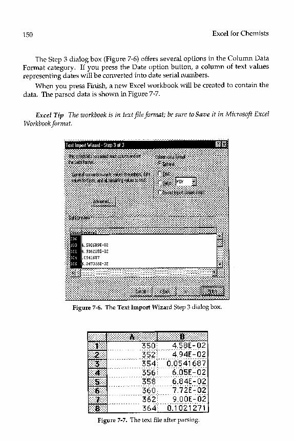
150 Excel for Chemists
The Step 3 dialog box (Figure 7-6) offers several options in the Column Data Format category. If you press the Date option button, a column of text values representing dates will be converted into date serial numbers.
When you press Finish, a new Excel workbook will be created to contain the data. The parsed data is shown in Figure 7-7.
Excel Tip The workbook is in textfile format; be sure to Save it in Microsoft Excel Workbook format.
Figure 7-6. The Text Import Wizard Step 3 dialog box.
354 0.0541687 3516 '6.1lSE-'ti'2 I 353 6.#4E-tl2 360' 7.72& (j2 I 362 'XQOE-02 _. .i._. . ...' ... 364' O.lti?b7i I
Figure 7-7. The text file after parsing.

Chapter 7 Importing Data Into Excel 151
USING TEXT TO COLUMNS
The Convert Text to Columns Wizard allows you to parse text within Excel. The Wizard is actuated by means of the Text to Columns... command in the Data menu.
The Text to Columns dialog boxes are essentially identical to those of the Text Import Wizard (see Figure 7-8). The data to be parsed must be in a single column.
Figure 7-8. The Text to Columns Step 1 dialog box with preview of data to be parsed.
The Step 3 dialog box contains an input box (not present in the Text Import Wizard) that allows you to specify where you want the parsed data to be placed. The default option overwrites the original data column.
FROMHARDCOPY (I%PER)T~ EXCEL Occasionally you’ll have data in hard copy tabular form (from a book, report,
correspondence, etc.). Unless the data set is very small, in which case it will be more efficient to enter the data manually, you’ll want to use some semi- automatic way to import the data from paper copy to Excel.
USING A SCANNER TO TRANSFER NUMERIC DATA TO EXCEL
You can use a scanner and a software program that performs optical character recognition to create a data file from hard copy. Once imported into Excel, the data may have to be manipulated to get it into a useable form. The following example shows how to record a simple Excel macro for converting scanned data with blank lines and other undesired features into useful columnar data.
Figure 7-9 shows scanned spectral data (absorbance values at 10 nm intervals from 500 nm to 680 nm for a metal ion at varying concentrations of a ligand)

152 Excel for Chemists
Figure 7-9. Spectral data imported from a monograph. (D. J. Leggett, Computational Methodsfir the Determination of Formation Constants, Plenum Press, New York, 1985)
copied from a monograph and imported into Excel. Because the data in the original copy was double-spaced, the scanner put the data in alternate rows of the spreadsheet. The data consists of (i) in Row 1, Row 9, etc., a row of data giving concentrations and path length, not necessary in our data table, (ii) in Row 3, Row 11, etc., eight values of absorbance measurements (for 500-570 nm) for one concentration of ligand, (iii) in Row 5, Row 13, etc., a second eight values of absorbance (580-660 nm), and in Row 7, Row 15, etc., the final two values of absorbance (670 and 680 run).
Of the 120 lines in data in the sheet, more than half need to be deleted. With a little bit of experience in recording macros, you can manually fix up the first lines of the data set while recording a macro, then let the macro do the rest. Chapter 13 provides information on how to record a macro. Here’s how to handle this example.
1. Before turning on the recorder, select the first row of data (Row 1).
2. Choose Record New Macro... from the Macro menu, and CONTROL+a (Windows) or OPTION+COMMAND+a (Macintosh) as the shortcut key.
3. Press the Relative Reference button.
4. Perform the following operations: (i) Delete the first two rows, (ii) Cut the second row of data and Paste it at the end of the first row of data, (iii) Cut the third row of data (two cells) and Paste at the end of the first row of data, (iv) select five rows and Delete, (v) select the next row of data, so that the previous operations will be repeated on the correct row when automated by using the macro.
5. Press the Stop Recording button or choose Stop Recording from the Macro submenu.
The recorded macro is shown in Figure 7-10.

Chapter 7 Importing Data Into Excel 153
Sub Macro1 () Macro1 Macro Macro recorded 2/8/00 by Dr. Billo Keyboard Shortcut: Option+Cmd+a
ActiveCell.Rows(“I :2”).EntireRow.Select Selection.Delete Shift:=xlUp ActiveCell.Offset(2, O).Range(“Al :Hl “).Select Selection.Cut ActiveCell.Offset(-2, 8).Range(“Al “).Select ActiveSheet.Paste ActiveCell.Offset(4, -8).Range(“Al :Bl “).Select Selection.Cut ActiveCell.Offset(-4, 1 G).Range(“Al “).Select
ActiveSheet.Paste ActiveCell.Offset(l , O).Rows(“l :!Y’).EntireRow.Select
Selection.Delete Shift:=xlUp ActiveCell.Rows(“l :I”).EntireRow.SeIect
End Sub
Figure 7-10. Recorded macro, with comments added.
0.8
0.7
0.6
0.5
0.4
0.3
0.2
01 .
Figure 7-11. Reformatted data.
00 l------ I I I
.
500 550 600 650
Figure 7-12. Chart created from imported data.

154 Excel for Chemists
The macro can be actuated by using CONTROL+a. If the cursor is placed on the first line of the original data, and CONTROL+a pressed, the data is automatically formatted and the cursor moved down to the next row. Thus, repeatedly pressing CONTROL +a will successively format each line of data.
Alternatively, the macro can be modified to go through the data table until all rows have been processed. To achieve this result, simply add the line of code
If ActiveCeli.Value c> “” Then GoTo Top
at the end and Top: at the beginning of the code. The complete data table is thus processed by a single CONTROL+a keystroke. A spreadsheet fragment showing some of the reformatted data is shown in Figure 7-11; Figure 7-12 is a chart of a portion of the imported data.
USING A SCANNER TO TRANSFER GRAPHICAL DATA TO EXCEL
You can use a scanner to convert graphs from strip chart recorders, published graphs or spectra, to digitized x, y data. Special software (e.g., Un- Scan-It from Silk Scientific, Inc., Orem UT 84059) is available for this purpose. First you scan the image using a scanner. Then you import the scanned image into the digitizing program. The program converts the scanned image into an x,y ASCII file.
SELECTINGEVERYNTH DATA POINT If you have imported a data file with a large number of data records (e.g.,
8000 data points) you may wish to work with a reduced data set, say, every fiftieth point. The following sections describe three ways you can create such a list: by using AutoFill to Fill Down a pattern, by using Excel’s Sampling tool, or by using a worksheet formula.
USING AUTOFILL
As you saw in Chapter 1, you can use AutoFill to Fill Down a pattern of selected cells. You can use this feature to select every Nth value in a range.
To create a list containing, for example, every tenth data point from the spectrophotometer data shown in Figure 7-7 (the complete data set covers the range 300-820 nm with an absorbance measurement every 2 nm), use the following procedure:
l In cell Cl, enter the formula =Al, and in Dl enter the formula = Bl. This will copy the first line of x,y data.
l Select (highlight) the range Cl :Dl 0 (1 row of values and 9 rows of empty cells).
l Use AutoFill to fill this pattern down to the end of the data, in row 236. This will return every 10th line of ~,y values.

Chapter 7 Importing Data Into Excel 155
0 While the range is still highlighted, Copy the values and Paste Special (Values). This is necessary because we are going to Sort the values in the next step.
While the range is still highlighted, choose Sort... from the Data menu and choose Ascending. This will cause the values to rise to the top of the range. Note that this procedure succeeds only because the x values are increasing monotonically. If neither the x values nor the y values change monotonically, add an adjacent column of integers 1, 2, 3,... and use this as the sortkey.
USING THE SAMPLING TOOL
You can use Excel’s Sampling tool, part of the Analysis ToolPak, to select every Mh value from a range. The Analysis ToolPak, which provides a range of statistical tools that you can use, is accessed by choosing Data Analysis... from the Tools menu. But since the Analysis ToolPak is an Add-In, the Data Analysis... command may not be present in the Tools menu (it’s normally located at the bottom of the menu). If the command is not present, choose Add- ins... from the Tools menu to display the Add-ins dialog box, check the box for Analysis ToolPak and press OK (Figure 7-13). You should now see the Data Analysis... command in the Tools menu. Choosing the Data Analysis... command displays the Data Analysis dialog box (Figure 7-14). Choose Sampling from the list of statistical tools to display the Sampling dialog box (Figure 7-15).
In the Input Range box, enter the range of x values. A deficiency of the Sampling tool is that it can sample in only one range at a time; if you have a column of x values and a column of y values, you’ll have to perform the sampling operation twice.
ternet Assistant WA
Figure 7-13. The Add-Ins dialog box.

156 Excel for Chemists
Two-F& With Replication mva: Two-Factor Without Replication
Figure 7-14. The Data Analysis dialog box.
Figure 7-15. The Sampling dialog box.
The Sampling tool can perform either random or periodic sampling. Press the button for periodic sampling and enter 10 as the value for the period.
There are three output options: sending the results to a new worksheet ply, to a new workbook, or to a specified range of cells on the active sheet. For this

Chapter 7 Importing Data Into Excel 157
example, we’ll send the result to start destination for the x values.
column C in the active sheet, so enter Cl as the
Finally, repeat the whole process to sample the range of y values.
USING A WORKSHEET FORMULA
Using the Sampling tool would be laborious if you needed to sample a data file with, for example, 17 columns: a column of x values and 16 columns of associated y values. You’d have to use the Sampling tool 17 times. In a case like this it would be preferable to have a formula, using relative references, that could be entered once, filled down to sample the column of x values, then filled right to create formulas that would sample each of the columns of y values. The following formulas illustrate how to do this.
Any of the four worksheet formulas described below can be used to select every Nth data point from a data table. All four utilize the INDEX(array, row - num,column - num) function to select an element from the array of data, but they use different methods to calculate the pointers row num and column num - - into the reference that contains the data.
l The first method uses names for the x and y data ranges; a separate worksheet formula must be entered for each column of data. The worksheet formula
=INDEX(XData,Nth*(ROW()-ROW(XData))+l)
when entered in cell T5 of Figure 7-16 and filled down yields the results shown in Figure 7-13. A similar formula is entered in cell U5 and filled down. XData and YData were defined as named ranges; the variable Nth contains the value 5.
l The second method uses a single worksheet formula that employs a mixed reference. The formula can then be copied into multiple columns. The formula
=INDEX(R$5:R$18,Nth*(ROW()-ROW(R$S:R$18))+1)
was entered in cell T5; then Fill Right was used to insert it into cell U5 to vield the formula
Upon application of Fill Down, the values shown in Figure 7-16 are produced.
l The third method uses an array formula that, because it involves both rows and columns, must be entered into the complete range of cells. The following array formula was entered in cells T5 :U7:
{=INDEX(Data,Nth*(ROW()-MIN(ROW()))+l ,COLUMN()-MIN(COLUMN())+l)}

158 Excel for Chemists
l The fourth method uses an array formula that can be entered into a single row of cells (here T5:U5) and then copied into the complete range of cells using either Fill Down or AutoFill:
{=INDEX(Data,Nth*(ROW()-ROW(Data))+l ,COLUMN()-MIN(COLUMN())+l)}
Figure 7-16. Using a worksheet formula to select every Nth data point.

8 ADDING CONTROLS
TO A SPREADSHEET
You can create what Microsoft calls a “custom form”. A custom form is a worksheet with one or more of the controls that are normally found in a dialog box - for example, option buttons to turn options on or off, or a list box to display a list from which the user can select an item. Thus you can create a user-friendly document that has many of the features usually found only in dialog boxes.
Most, but not all, of the controls that you have seen in Excel’s dialog boxes can be installed on a worksheet. These controls return a value to a worksheet cell (the cell link). You can then use this value in worksheet formulas.
YOUCAN ADDOPTION BUTTONS, CHECK BOXES, LIST BOXESANDOTHERCONTROLSTOAWORKSHEET
The controls that can be installed on a worksheet to return a value to a worksheet cell are an option button, a check box, a list box, a drop-down list box (somet~es called a combo box), a scroll bar and a spinner. In addition, you can install a group box, which does controls, usually option buttons.
not return a value but is used to group related
OPTION BUTTON
An option button is used to select one of a group of options. When related option buttons are placed within a group box, only one button of the group can be selected. Use option buttons when only one of several possibilities is allowed at any given time.
CHECK BOX
A check box is used to turn an option on or off. Use check boxes when several possibilities are allowed at any given time.
159
Excel for Chemists: A Comprehensive Guide. E. Joseph BilloCopyright 2001 by John Wiley & Sons, Inc.
ISBNs: 0-471-39462-9 (Paperback); 0-471-22058-2 (Electronic)

160 Excel for Chemists
LIST BOX
A list box displays a list of items. Several of the items in the list are visible in the box; the user scrolls up or down to display the rest of the list, then chooses an item.
COMBO BOX
A drop-down list box (combo box) displays a list of items. Initially only one item is visible in the window; the user presses the drop-down button to display the rest of the list, then chooses an item.
SCROLL BAR
A scroll bar, with buttons and a slider, permits the user to increase or decrease a value in a worksheet cell. Maximum and minimum values can be set for the value returned by the scroll bar. A Scroll Bar can be installed either horizontally or vertically.
SPINNER
A spinner is a button with an up arrow and a down arrow that permits the user to increase or decrease a value in a worksheet cell. Maximum and minimum values can be set for the value returned by the spinner.
HOW TOADDACONTROLTOAWORKSHEET Adding a control to a worksheet is a three-step process: first, you display
the Forms toolbar (Figure 8-l); then you use the Forms toolbar to draw the desired control; finally, you set the control properties. For example, for a list box, the control properties are (i) the range of values to be displayed in the list and (ii) the cell link, the cell to which the list box returns a value. Follow the procedure in the following box.
Figure 8-l. The Forms toolbar

Chapter 8 Adding Controls to a Spreadsheet 161
Each control has a title, e.g., Check Box 1, associated with it. The titles are numbered sequentially as you add them; for example, if you add a list box, then three option buttons, then a check box, they will have titles Option Button 2, Option Button 3, Option Button 4, Check Box 5 (the list box doesn’t have a title that you can see). You can select the title text and change it.
Almost always you will place several related option buttons within a group box and link each option button to the same cell. (The best pr~edure the group box first, then add the option buttons wi .thin the group box.)
is to add
Table 8-l provides details on control properties.
CONTROL PROPERTIES
You set the properties of a control by choosing Control,., from the Format menu or Format Control... from the shortcut menu to display the Format Control dialog box for the specific control, then choose the Control tab. Some control properties function only when the control is used with a macro. You can set these control properties but they will have no effect on a control installed on a worksheet.

162 Excel for Chemists
Table 8-l. Control Properties
Check Box Cell Link: a reference to a cell that returns the state of the check box: TRUE if the box is checked, FALSE if unchecked. This logical argument can be used in a formula.
Option Button Cell Link: a reference to a cell that returns the number of the option button that is selected. Only one option button within a group box can be selected (pressed) at any time. The cell link re- turns the number of the option button within the group (e.g., 1, 2 or 3) not the number that appeared in the original title (e.g., Option Button 7, Option Button 8, Option Button 9).
List Box Input Range: a reference to a range of cells whose values will be displayed in the list box.
Cell Link: a reference to a cell that refurns a value that is the relative position of the selected item in the list. This value can then be used in a formula to return a result based on the selected item in the list.
Selection Type: you must use Single when a list box is installed on a worksheet.
Combo Box Input Range: a reference to a range of cells whose values will be displayed in the drop-down list box.
Cell Link: a reference to a cell that returns the relative position of the selected item in the list.
Scroll Bar Minimum Value: the minimum value that the scroll bar can re- turn (corresponds to the top of a vertical scroll bar or the left end of a horizontal scroll bar).
Maximum Value: the rn~~ value that the scroll bar can return (corresponds to the bottom of a vertical scroll bar or the right end of a horizontal scroll bar).
Incremental Change: the amount the scroll slider button moves when an arrow at either end of the scroll bar is clicked. The de- fault value is 1.
Page Change: the amount the scroll slider button moves when you click between the scroll button and one of the scroll arrows. The default value is 10.
Cell Link: a reference to a cell that returns the current value of the scroll bar. This number can be used in a formula to return a result based on the position of the scroll slider button in the scroll bar.
Spinner ?he control properties for a spinner are the same as those for a scroll bar, but spinners do not have a Page Change property.

Chapter 8 Adding Controls to a Spreadsheet 163
A LIST BOX ON A WORKSHEET As a simple first exercise, we’ll create a list box that displays a list of
items. The list that will be displayed consists of the names of the months of the year. When you select a particular month from the list, the list box returns a number from 1 to 12, the relative position of the selected item in the list.
First, create a range of cells containing the list to be displayed. Fill the range Al :A1 2 (use a different worksheet than the one where you’re going to install the list box) with the text January, February, etc. You can use AutoFill to do this.
To install the list box on a worksheet, follow the procedure outlined earlier in this chapter. First, display the Forms toolbar. Click on the List Box bu~on (second from the right in the top row in Figure 8-l) and use the mousepointer to draw the outline of a list box. While the list box is still selected (has handles around it), choose Control... from the Format menu. In the Input Range box, enter the external reference to the range of cells containing the list to be displayed. In the Cell Link box, enter a cell reference, e.g., C5, then press OK.
To make the list box active, click on any cell in the worksheet. The handles around the list box will disappear.
Figure 8-2. A list box installed on a worksheet. The cell link is cell C5.
The list box should now display the months of the year, as shown in Figure 8-2. When you select an item from the list, the Cell Link will return the number of the selected item. You can use the cell link value in a formula.
To select the list box for moving or re-sizing, click on it once while holding down the CONTROL key.
A DROP-DOWN LIST BOX ON A WO~SHEET Figure 8-3 shows a drop-down list box that is used to display a subset of a
list. This drop-down list box displays, from a list of names and telephone

164 Excel for Chemists
numbers, the subset of names that begin with a particular letter or string. The user can display all the names that begin with the letter “D”, or “McD”, for example. VVhen the user chooses a name from the subset displayed in the drop- down list box, that person’s telephone number is displayed in a cell.
The advantage of using the drop-down list box rather than a simple list box is that the box automatically sizes to fit the number of values displayed.
In this example names, addresses and telephone numbers are listed in columns A, B and C of the worksheet. The range A2:Al39 was assigned the name Names, C2:C139 the name Phones. The list of names was sorted in alphabetical order.
Figure 8-3 shows the list box displaying the sublist of names beginning with the letter D. To select the subset to be displayed, the user enters a letter or string in cell F2.
The reference SubListStart, in cell G2, contains the formula =~ATCH(Letter&“*“,Names,O)
This formula returns the relative position of the first item in the list that matches the input string. In our example, the first name that begins with D is the 35th item in the list in column A. The reference SubListLength, in cell H2, contains the array formula
{=SUfVl(l *(LEFT(Names,LEN(Letter))=Letter))} This formula returns the number of items in the list that match the input
string. These two formulas are combined in the formula =OFFSET($A$l ,SubListStart,O,SubListLength,l)
to return a reference to the cells containing the sublist. This formula was entered as a named formula (using Define Name) and given the name DropList. In fact, all the formulas in this example can be entered as named formulas.
Figure 8-3. A drop-down list box displaying a subset of a list. The cell link is cell 12.

Chapter 8 Adding Controls to a Spreadsheet 165
F~ally, using Control... from the Format menu, DropList was entered as the reference for the Input Range of the list box and cell 12 as the Cell Link.
The formula to return the telephone number corresponding to the name selected from the list box
=INDEX(Telephones,SubListStart+CellLink-I)
was entered in cell H6. Figure 8-4 illustrates the final result.
Telephone a: 555-5618
Figure 8-4. A drop-down list box used to return a telephone number.
OPTION BUTTONS AND A DROP-DOWN LIST Box This example illustrates the use of option buttons in comb~ation with the
drop-down list of the preceding example. The option buttons are used to specify whether to display the address or telephone number corresponding to the selected name.
Two option buttons were positioned inside a group box (see Figure 8-5) and the titles “Option Button 2” and “Option Button 3” were changed to “Address” and “Phone”, respectively. The Cell Link for the two buttons was cell J 2, which was given the name Colu~nOffset.
Figure 8-5. A drop-down list box used to return address or telephone number.

166 Excel for Chemists
ColumnOffset is used in the following formula, in cell L8, to specify whether to return either the address (in column B of the range DirectoryTable, or the telephone number in column C of DirectoryTable:
=INDEX(DirectoryTable,SubListStart+CeIILink-1 ,ColumnOffset+l)

PART III
SPREADS1 IEET MATHEMATICS
Excel for Chemists: A Comprehensive Guide. E. Joseph BilloCopyright 2001 by John Wiley & Sons, Inc.
ISBNs: 0-471-39462-9 (Paperback); 0-471-22058-2 (Electronic)

9 SOME MATHEMATICAL TOOLS
FOR SPREADSHEET CALCULATIONS
This chapter describes some mathematical methods that are useful for spreadsheet calcula~ons. For the most part, they are methods that are applicable to tables or arrays of data.
LOOKING UP VALUES IN TABLES The VLOOKUP(/ookup value, - array, co/umnJ7dex~num,
match- type-logical) worksheet function is useful for obtaining values from tables This section shows how to use VLOOKUP to obtain a value both from a one-way table and a two-way table.
GETTING VALUES FROM A ONE-WAY TABLE
The spreadsheet shown in Figure 9-1, containing a list of element symbols and atomic weights, is part of a one-way table (the table entries extend down to row 110). In a one-way table, the lookup values occupy a single row or column of the table (here, the lookup values are found in column B).
We want to obtain the atomic weight of a particular element from the table, in order to use it in a formula. The formula =VLOOKUP(symbol,$B$2:$D$110,2,O) returns the atomic weight corresponding to symbol. The formula =VLOOKUP(symbo~,$B$2:$D$l10,3,0) returns the electron configuration.
1.00797 131 4.0026 ls2 , I/ ". .
LI . 6.939 [He] 231 : ? < Be 9.0122 [He] Z&ii ‘ ~ E 10.811 [He] 2kiipl c 12.01115 [He] 292 2p2
Figure 9-l. Portion of a data table of the elements.
169
Excel for Chemists: A Comprehensive Guide. E. Joseph BilloCopyright 2001 by John Wiley & Sons, Inc.
ISBNs: 0-471-39462-9 (Paperback); 0-471-22058-2 (Electronic)

170 Excel for Chemists
Figure 9-2. Portion of a data table of the elements.
Mien you use VLOOKUP, you must always “look up” in the first column of the defined database and retrieve associated ~formation from a column to the right in the same row; you cannot VLOOKUP to the left, for example. In the table shown in Figure 9-2, you cannot use VLOOKUP to return the element name corresponding to symbol. If you want to perform a lookup to the left of, or above, the lookup value, you can either construct your own lookup-type function using the MATCH function (see later in this chapter) or use the LOOKUP function.
GETTING VALUES FROM A TWO-WAY TABLE
A two-way table has two lookup values, usually in the lef~ost column and in the top row. The value to be returned from the table is the value located at the intersection of the row and column containing the two lookup values.
Once again we cm use VLOOKUP to obtain the value from the table. In the preceding example, the value used for the column-index-num argument of VLOOKUP was the fixed value 2, because we are always going to be returning a value from column 2 of array. In the two-way table example shown in Figure 9-3, column-index-n~rn is a variable; we must determine by means of an expression the column from which the desired value is to be returned. The MATC t-l expression can be used to obtain the relative column number in the table corresponding to the lookup value.
To find the value in the table for T = 950°F and P = 5000 psia, the expression
=VLOOKUP(B44,$A$4:$P$34,~ATC~(B4~,$B$3:$P$3,1)+1 ,I)
where the T and P lookup values are entered in cells B44 and 845 respectively, returns the value 0.035 for the viscosity. The same formula, using names instead of references,
=VLOOKUP(T,T-Table,~ATC~(P,P-Ro~,l)+l ,l)
returns the value for the viscosity.

z c3
m
i*J
‘u
0 r cl
cn
ee
I?
F .::::.
.s
:: .,:
.*.
A::
:;‘i::
;:...
fgg
T.&J
/
p .,.
,.:
: :, ‘:’ . . ::
.: ,. .: . . . .
y . . . ..:
. . $g
gg
:::@
$g>
&: :.s
.:::.;
. . . . . >
.,:.:.
:c
g&
ri~~~
,.i @
“#
@J
figj

172 Excel for Chemists
Iookup~value. The x values in the array must be in ascending order. Thus, for any lookup value, you can use MATCH to find the pointer to the position of ~0, the value of x in the table that is less than or equal to the lookup value, and then use this pointer in the INDEX function to return values for x0, xl, yo and ~1, as in the following formulas:
position
x0
Xl
YO =INDEX(YValues,position)
Y-l
The preceding formulas were applied in the example shown in Figure 9-4, to perform table lookup with linear interpolation in the simple data table in A5:B8. The intermediate values shown in B13:BW in Figure 9-5 were used to develop, in a stepwise manner, the follow~g ~terpolation formula used in B18.
=y~O+(LookupValuemx~O)*(y~l~y~O)/(x~l~x~O)
A chart of the data with some interpolated values is shown in Figure 9-6.
Figure 9-4. Data table for interpolation.
Figure 9-5. Intermediate values for stepwise development of interpolation formula.

Chapter 9 Some Ma~ematical Tools for Spreadsheet Calculations 173
700
600
500
400
300
200
100
Figure 9-6. Chart showing some interpolated values
The formulas for the ~termediate values in B13:B17 can be copied and pasted into the interpolation formula in B18 to create a single “megaformula” (all in one cell, of course):
=INDEX(YValues,MATCH(LookupValue,XValues,l))+(LookupValue-lNDEX( XValues,MATCH(LookupValue,XValues,l)))*(lNDEX(YValues,MATCH( LookupValue,XValues,l)+l)-INDEX(YValues,MATCH(LookupValue, XValues,l)))l(lNDEX(XValues,MATCH(LookupValue,XValues,l)+l)- lND~X(XValues,MATCH(LookupValue,XValues,~)))
If the x values in the data table are in descending order, the match-type argument in the MATCH function must be changed to -1.
INTERP~LAT~~NMETH~DS: CUBIC Simple linear interpolation is not always adequate for data tables with
extensive curvature. Cubic i~~e~p~~~~i~# uses the values of four adjacent data points to evaluate the coefficients of the cubic equation y = a + bx + CA? + dx3.
A compact and elegant implementation of cubic ~terpolation in the form of an Excel 4.0 Macro Language custom function was provided by Or& A slightly modified version, in VBA (Visual Basic for Applications) language, is provided here (Figure 9-7). The syntax of the custom function is Cubiclnterp(~~~~~-x~, known_ys, x-value).
William J. Orvis, Excel 4 for Scientists alzd ~~gi~eers~ Sybex Inc,, Alameda, CA, 1993.

174 Excel for Chemists
Function Cubiclnterp(XValues, YValues, X) ’ Performs cubic interpolation, using an array of XValues, YValues. ’ The XValues must be in ascending order. ’ Based on XLM code from “Excel for Chemists”, page 239, ’ which was based on W. J. On/is’ code. Row = App~icat~on.Mat~h(X, XValues, 1)
If Row c 2 Then Row = 2 If Row > XValuesCount - 2 Then Row = XValues.Cou~t - 2
Forl=Row~~ToRow+2 Q=l
ForJ=Row-1 ToRow+ If I <> J Then Q = Q * (X - XValues(J)) / (XValues(l) - XValues(J))
Next J Y = Y + Q * YValues(l)
Next I Cubiclnterp = Y End Function
Figure 9-7. Cubic interpolation function macro.
The cubic interpolation function can be used to produce a smooth curve through data points. Figure 9-8 illustrates a portion of a spreadsheet with experimental spectrophotometric data taken at 5 nm intervals in columns A and B (the data are in rows 6-86), and a portion of the interpolated values, at 1 nm intervals, in columns C and D. The formula in cell D24 is
= Cubiclnterp ($A$6:$A$86,$B$6:$B$86,C24)”
The smoothed curve through the data points is illustrated in Figure 9-9.
Figure 9-8. kterpolation by using a cubic interpolation unction macro.

Chapter 9 Some Mathematical Tools for Spreadsheet Calculations 175
0.600
s 0.590
i 0.580
5: 0.570
0.600
Q) 0.590 ii! 2 0.580
ti 2 0.570
a 0.560
0.550 390 400 410
Wavelength, nm
420
a 0.560
0.550
Wavelength, nm
420
Figure 9-9. (Left) Chart created using data points onl r
. interpolated using a cubic
(Right) Chart with smooth curve interpo ation function.
The cubic interpolation function forces the curve to pass through all the known data points. If there is any experimental scatter in the data, the result will not be too pleasing, A better approach for data with scatter is to find the coefficients of a least-squares line through the data points, as described in Chapter 11 or 12.
NUMERICAL DIFFERENTIATION The process of finding the derivative or slope of a function is the basis of
di~~~~ti~Z ~~1~~1~s. Since you will be dealing with spreadsheet data, you will be concerned not with the algebraic differentiation of a function, but with obtaining the derivative of a data set or the derivative of a worksheet formula by numeric methods.
Often a function depends on more than one variable. The p~~ti~Z d~ri~~ti~e of the function F(x,y,z), e.g., SF/&x, is the slope of the function with respect to x, while y and z are held constant.
FIRST AND SECOND DERIVATIVES OF A DATA SET
The simplest method to obtain the first derivative of a function represented by a table of x, y data points is to calculate Ay/Ax. The first derivative or slope of the curve at a given data point x~, yn can be calculated using either of the following formulas:
4! slope = ti = Yn+l -Yn %z+l -%I
(9-2)
slope = Yn - Yn-1 x7-l - %-1
P-3)

176 Excel for Chemists
Figure 9-10. First derivative of titration data, near the end-point.
The second derivative, d2y/dx 2, of a data set is calculated in a similar manner, namely by calculating A(Ay/~) /AX.
Calculation of the first or second derivative of a data set tends to emphasize the “noise” in the data set; that is, small errors in the measurements become relatively much more important.
Points on a curve of X, y values for which the first derivative is either a maximum, a minimum or zero are often of particular importance and are termed critical points.
The spreadsheet shown in Figure 9-10 uses pH titration data to illustrate the calculation of the first derivative of a data set .
1.500 2.000 2.500
V, mL
Figure 9-11. First derivative of titration data, near the end-point.

Chapter 9 Some Mathematical Tools for Spreadsheet Calculations 177
Figure 9-12. Second derivative of titration data, near the end-point.
Since the derivative has been calculated over the finite volume AV = V,+l - Vn, the most suitable in Figure 9-10, is:
volume to use when plotting the ApH/AV values, as shown
V v,+1+ vn
average = 2 P-4)
The maximum in ApH/AV indicates the location of the inflection point of the titration (Figure 9-11). The second derivative, A( ApH/AV) /AV, which is calculated by means of the spreadsheet shown in Figure 9-12, can be used to locate the inflection point more precisely. The second derivative passes through zero at the inflection point. Linear interpolation can be used to calculate the point at which the second derivative is zero (Figure 9-13).
2000 r
V, mL
Figure 9-13. Second derivative of titration data, near the end-point.

178 Excel for Chemists
There are more sophisticated equations for numerical differentiation. These equations use three, four or five points instead of two points to calculate the derivative. Since they usually require equal intervals between points, they are of less generality. Their main advantage is that they minimize the effect of “noise”.
DERIVATIVES OF A FUNCTION
The first derivative of a formula in a worksheet cell can be obtained with a high degree of accuracy by evaluating the formula at x and at x + AX. Since Excel carries 15 significant figures, AX can be made very small. Under these conditions AF/Ax approximates d.F/dx very well.
The spreadsheet fragment shown in Figure 9-14 illustrates the calculation of the first derivative of a function (F = x3 - 3x2 - 130x + 150) by evaluating the function at x and at x + Ax. Here a value of Ax of 1 x 10mg was used; alternatively Ax could be obtained by using a worksheet formula such as =I E-9*x. For comparison, the first derivative was calculated from the exnression from diffeiential calculus: F’ = 3x2 - 6x - 130.
1
The Excel formulas in cells B12, Cl 2, D12 and El 2 are
= t*xA3+u*xA2+v*x + w
= t*(x+delta)A3 +u*(x+delta)A2 +v*(x+delta) + w
Figure 9-14. Calculating the first derivative of a function.

Chapter 9 Some Mathematical Tools for Spreadsheet Calculations 179
=(C12-B12)Melta
=3*t*xA2+2*u*x+v
Figure 9-15 shows a chart of the function and its first derivative.
800
600
400
4s z 200 ‘CI
ti 0 u,
-200
-400
-600
IL I. I I -10 -5 0
X
Figure 945. The function F = x3 - 3x2 - 130x + 150 and its first derivative.
NUMERICAL INTEGRATION A common use of numerical integration is to determine the area under a
curve. We will describe three methods for determining the area under a curve: the rectangle method, the trapezoid method and Simpson’s method. Each involves approximating the area of each portion of the curve delineated by adjacent data points; the area under the curve is the sum of these individual segments.
The simplest approach is to approximate the area by the rectangle whose height is equal to the value of one of the two data points, illustrated in Figure 9- 16.
As the x increment (the interval between the data points) decreases, this rather crude approach becomes a better approximation to the area. The area under the curve bounded by the limits xinitial and xfinal is the sum of the individual rectangles, as given by equation 9-5.
area = Z y&i+1 - xi) P-5)

180 Excel for Chemists
10 I
Simpson’s Rule method
7
6
* 5
-
1.5 2
X
1 Figure 9-16. Graphical illustration of methods of calculating the area unaer a curve.
2.5
For a better approximation you can use the average of the two y values as the height of the rectangle. This is equivalent to approximating the area by a trapezoid rather than a rectangle. The area under the curve is given by equation 9-6 .
area = C yi +:i+l (Xi+1 - Xi) P-6)
Simpson’s rule approximates the curvature of the function by means of a quadratic equation. To evaluate the coefficients of the quadratic requires the use of the y values for three adjacent data points. The x values must be equally spaced.
area = c Yi + 4Yi+l + Yi+2
6 (Xi+1 - Xi) P-7)
AN EXAMPLE: FINDING THE AREA UNDER A CURVE
The curve shown in Figure 9-17 is the sum of two Gaussian curves, with position and standard deviation of = 90, CT = 10 and ~=130, CT = 20, respectively. The equation used to calculate each Gaussian curve is
Y= expf -(x - p)2/202]
cn/5i P-8)

Chapter 9 Some Mathematical Tools for Spreadsheet Calculations 181
50 100 150 200
X
Figure 9-17. A curve that is the sum of two Gaussian curves.
The area of each Gaussian curve is equal to 1.000; thus the total area under the curve shown in Figure 9-17 is 2.000. The Excel formula used to calculate y is as follows (m is the position u and s is the standard deviation 0):
=EXP(-O.~*((X-curvl m)!curvl s)/\2)/(SQRT(Z*Pl())*curvl s)+EXP(- 0.5” ((x-curv2 m)/curv2 s)A2)/(SQRT(2*Pl())*cu~2 s)
The area under the curve, between the limits x = 50 and x = 200, was calculated by using each of the preceding equations (9-5, 9-6 and 9-7): the rectangular approximation, the trapezoidal approximation and Simpson’s rule. In each case a constant x increment of 10 was used. A portion of the spreadsheet is shown in Figure 9-18.
The formulas in row 9, used to calculate the area increment, are as follows:
=I O”F9 (rectangular approximation)
=I O*(F8+F9)/2 (trapezoidal approximation)
=I O*(F8+4*F9+F10)/6 (Simpson’s rule)
CL00562 ii.05621 " __ CL03 0.02507 0.25073 ty.15 a.04259 ._ 0.4259+,, 0.33
054 347 ;, 834‘ .,
0.08#07 0.24751 '0.37'687
cm3067 0.30673 0.36633 0.30464
Figure 9-18. Portion of a spreadsheet for calculating the area under a curve.

182 Excel for Chemists
The area increments were summed and the area under the curve, calculated by the three methods, is shown in Figure 9-19. All three methods of calculation appear to give acceptable results in this case.
Figure 9-19. Area under a curve, calculated by three different methods.
DIFFERENTIAL EQUATIONS Certain chemical problems, such as those involving chemical kinetics, can be
expressed by means of differential equations. For example, the coupled reaction scheme
kl k3 A-Be c
k2 k4 results in the simultaneous equations
aA1 - = -kl[A] + k;lfB] dt
dEBI - = kl[A] - k2[B] - k$B] + k4[C] dt
4Cl - = k$B] - k&] dt
To “solve” this system of simultaneous equations, we want to be able to calculate the value of [A], [B] and [C] for any value of t. For all but the simplest of these systems of equations, obtaining an exact or analytical expression is difficult or sometimes impossible. Such problems can always be solved by numerical methods, however. Numerical methods are completely general. They can be applied to systems of differential equations of any complexity, and they can be applied to any set of initial conditions. Numerical methods require extensive calculations but this is easily accomplished by spreadsheet methods.
In this chapter we will consider only ordinary differential equations, that is, equations involving only derivatives of a single independent variable. As well, we will discuss only initial-value problems - differential equations in which ~formation about the system is known at t = 0. Two approaches are common: Euler’s method and the Runge-Kutta (RK) methods.

Chapter 9 Some Mathematical Tools for Spreadsheet Calculations 183
EULER’S METHOD
Let us use as an example the simulation of the first-order kinetic process A --I, B with initial concentration Co = 0.2000 mol/L and rate constant k = 5 x 10” WI s l We’ll simulate the change in concentra~on vs. time over the interval from t =
0 to t = 600 seconds, in increments of 20 seconds.
The differential equation for the disappearance of A is d[A]/dt = -k[A]. Expressing this in terms of finite differences, the change in concentration A[A] that occurs during the time interval from t = 0 to t = At is A[A] = -k[A]At. Thus, if the concentration of A at t = 0 is 0.2000 M, then the concentration at t = 0 + At is [A] = 0.2000 - (5 x 10*3)(0.2000)(20) = 0.1800 M. The formula in cell 87 is
=B6-k*BG*DX.
The concentration at subsequent time intervals is calculated in the same way.
The advantage of this method, known as Euler’s method, is that it can be easily expanded to handle systems of any complexity. Euler’s method is not particularly useful, however, since the error introduced by the approximation d[A]/dt = A[A]/At is compounded with each additional calculation. Compare the Euler’s method result in column B of Figure 9-20 with the analytical expression for the concentration, [A]t = [A]Oewkt, in column C. At the end of approximately one half-life (seven cycles of calculation in this example), the error has already increased to 3.6%. Accuracy can be increased by decreasing the size of At, but only at the expense of increased computation. A much more efficient way of increasing the accuracy is by means of a series expansion. The Runge- Kutta methods, which we describe next, comprise the most commonly approach.
0.1482 0.1341
Figure 9-20. Euler’s method.
used

184 Excel for Chemists
THE RUNGE-KUTTA METHODS
The Runge-Kutta methods for numerical solution of the differential equation dy/dx = F(x, y) involve, in effect, the evaluation of the differential function at intermediate points between xi and xi+l. The value of yi+l is obtained by appropriate summation of the intermediate terms in a single equation. The most widely used Runge-Kutta formula involves terms evaluated at xi, xi + Ax/2 and xi + AX. Thefourth-order Runge-Kutta equations for dy/dx = F(x, y) are
Tl + 2T2 + 2T3 + T4 Yi+l = yi +
6 (9-9)
where Tl = F (xi yi) AX (9-10)
T2 F( Ax Tl - - xi+- ,yi+- Ax 2 2 >
T3 Ax T2 - - F( xi +-, yi +- 2 2 ) AX
(9-11)
(9-12)
T4 = F (Xi + AX, J/i + T3) AX (9-13)
If more than one variable appears in the expression, then each is corrected by using its own set of T1 to T4 terms.
The spreadsheet in Figure 9-21 illustrates the use of the RK method to simulate the first-order kinetic process A + B with initial concentration [A]0 = 0.2000 and rate constant k = 5 x 10m3. Th e 1 d’ff erential equation is d[A]f/dt = -k[A]t. This equation is one of the simple form dy/dx = F(y), and thus only the yi terms of T1 to T4 need to be evaluated. The RK terms (note that T1 is the Euler method term) are shown on the following page.
.., . , , , . , . , , , : , . . ‘.
___31
” : ,,’ , , ,,I,’ ‘, : . , : ; . ,, ‘:.,,. . . . “ .
.’ k
‘,.. 1 : EF
: : : . . 1
: . , , , , ‘,. . . . : , , , : ,’ . . ,‘,
c.1, .’ . , . ” : . ‘.‘..
,‘, , . . . . : : y.,.,
..i , : . : . ..l .(. . : . : : . : . , . ,
, . . / ::‘, , , . I , , . , . : .’ &ye-K&a +im
: ,:.. :, .: . . ., ,’ ,2’, ::, . , j: , : ,‘, : . .V’ . , , ,.. .'.' ..” . , rate constant= 5.OE-03 k) '. ,. ':', ,. .., ;. '.. ,'d 3 . . time increment= 20 WO
" . . . . c,, 4"' " . . ',,. . . ,, : ; I.: : " 'T ., .:
TA2 TA3 TA4
-0.0200 -0.0190 -0.0191 -0.0181 -0.0172 -0.0172 -0.0164
-0.0164 -0.0156 -0.0156 -0.0148
ml e’[-kt) 0.2000 0.2000 tl.1810 0.1810 0.1637 0.1637 0.1482 0.1482
.-l;~:@:‘. 30 -0.0148 -0.0141 -0.0141 -0.0134 0.1341 0.1341 qjj/i/:g 1 00 -0.0134 -0.0127 -0.0128 -0.0121 0.1213 0.1213 ;1_2i.::" 1 20 -~Jjl 21 -0.0115 -0.0116 -0.0110 0.1098 0.1098 ,.,,.:“:p&~:~;: 1 40 -O.#llO -0.0104 -0.0105 -0.0099 0.0993 0.0993 + " " "
Figure 9-21. The Rung-Kutta method.

Chapter 9 Some Mathematical Tools for Spreadsheet Calculations 185
l-1 = -kfA]t Ax (9-14)
l-2 = -k([A]t + Q/2) Ax (9-15)
T3 = -k([A]t + 7’2/2) Ax (9-16)
T4 = -k([A]t + I-3) Ax (9-17)
The RK equations in cells 87, C7, 07, E7 and F7, respectively, are:
=-k*FG*DX
=-k*( FG+TAI l2)“DX
=-k*( F6+TA2/2)*DX
=-k*(FG+TA3)*DX
If you use the names TAl ,..*, TA4, TBl,..., TB4, etc., you’ll find that (i) the nomenclature is expandable to systems requiring more than one set of Runge- Kutta terms, (ii) the names are accepted by Excel, whereas Tl is not a valid name, and (iii) you can use AutoFill to generate the column labels TAI ,..., TA4.
Compare the RK result in column F of Figure 9-21 with the analytical expression for the concentration, [A]t = [A]gemkt, in column G. After one half-life (row 13) the RK calculation differs from the analytical expression by only 0.00006%. (Compare this with the 3.6% error in the Euler method calculation at the same point.) Even after 10 half-lives (not shown), the RK error is only 0.0006%.
If the spreadsheet is constructed as shown in Figure 9-21, you can’t use a formula in which a name is assigned to the concentration array in column F. This is becasue the formula in 87, for example, will use the concentration in F7 instead of the required F6. An alternative arrangement that permits using a name for the concentration [A]t is shown in Figure 9-22. Each row contains the concentration at the beginning and at the end of the time interval. The name A t -
Figure 9-22. Alternative spreadsheet layout for the Runge-Kutta method.

186 Excel for Chemists
can now be assigned to the array of values in column B; the former formulas (now in cells C7-G7) contain A-t in place of F6, and cell B7 contains the formula =G6.
In essence, the fourth order Runge-Kutta method performs four calculation steps for every time interval. In the solution by Euler’s method, decreasing the time increment to 5 seconds, to perform four times as many calculation steps, still only reduces the error to 0.9% after 1 half-life.
ARRAYS,MATRICES ANDDETERMINANTS Spreadsheet calculations lend themselves almost automatically to the use of
arrays of values. As you‘ve seen, arrays in Excel can be either one- or two- dimensional. For the solution of many types of problem, it is convenient to manipulate an entire rectangular array of values as a unit. Such an array is termed a rn~~~i~. (In Excel, the terms “range”, ” array ” and “matrix” are virtually interchangeable.) An m x n matrix (m rows and n columns) of values is illustrated on the following page-

Chapter 9 Some Mathematical Tools for Spreadsheet Calculations 187
:
Qn2 *.*
. : 0
arnn
The values comprising the array are called matrix elements. Mathematical operations on matrices have their own special rules.
A s9~~~e rn~t~i~ has the same number of rows and columns. If all the elements of a square matrix are zero except those on the main diagonal (all,
a22,-9, @nn ), the matrix is termed a diagonal matrix. A diagonal matrix whose diagonal elements are all 1 is a unit matrix.
A matrix which contains a single column of m rows or a single row of n columns is called a nectar.
A determinant is simply a square matrix. There is a procedure for the numerical evaluation of a determinant, so that an N x N matrix can be reduced to a single numerical value. The value of the determinant has properties that make it useful in certain tests and equations. (See, for example, “Solving Sets of Simultaneous Linear Equations” in Chapter 10.)
AN INTRODUCTION TO MATRIX ALGEBRA
Matrix algebra provides a powerful method for the manipulation of sets of numbers. Many mathematical operations - addition, subtraction, multiplication, division, etc. - have their counterparts in matrix algebra. Our discussion will be limited to the manipulations of square matrices. For purposes of illustration, two 3 x 3 matrices will be defined, namely
and
s
V
Y
t 1 I 2
w = 0
z 3
0
3
2
2
3
1 1
The following examples illustrate addition, subtraction, multiplication and division using a constant.
Addition or subtraction of a constant:

188 Excel for Chemists
Multiplication or division by a constant: qA =
Addition or subtraction of two matrices (both must contain the same number of rows and columns):
A+B=
Performing matrix algebra with Excel is very simple. Let’s begin by assuming that the matrices A and B have been defined by selecting the 3R x 3C arrays of cells containing the values and naming them by using Define Name. To add a constant (e.g., 3) to matrix A, simply select a range of cells the same size as the matrix, enter the formula =A+3, then press COMM~N~+R~TU~ or C~NTR~L+SHI~+RETU~ (Mac~tosh) or CONTROL+SHI~+ENTER (Widows). Subtraction of a constant, multiplication or division by a constant, or addition of two matrices also is performed by using standard Excel algebraic operators.
Multiplication of two matrices can be either SC~Z~~ multiplication or ~~c~~~ multiplication. Scalar multiplication of two matrices consists of multiplying correspond~g elements, i.e.,
Thus it’s clear that both matrices must have the same dimensions m x n. Scalar multiplication is commutative, that is, A*B = B*A
The vector multiplication of two matrices is somewhat more complicated:
AwB= ~~ % ~I*[~ ; :;;[
ar+bu+cx as+bv+cy at+bw+cz
dr+eu+ fx ds+ev+fi dt+ew+ fz gr+hu+ix gs+hv+iy gt+hw+iz
]
Vector multiplication is not commutative, that is A*B # B-A.
Vector multiplication can be accomplished easily by the use of one of Excel’s worksheet functions for matrix algebra, ~~~LT( ~~~~~~7, ~~f~~x2). For the matrices A and B defined above,

Chapter 9 Some Mathematical Tools for Spreadsheet Calculations 189
Two matrices can be B has columns.
vector-multiplied when A has the same number of rows
B-A =
Vector multiplication of two matrices is possible only if the matrices are conformable, that is, if the number of columns of A is equal to the number of rows of B. The opposite condition, if the number of YOWS of A is equal to the number of columns of B, is not equivalent. The following examples, involving multiplication of a matrix and a vector, illustrate the possibilities:
MMULT (4 x 3 matrix, 3 x 1 vector) = 3 x 1 result vector MMULT (4 x 3 matrix, 1 x 4 vector) = #VALUE! MMULT (1 x 4 vector, 4 x 3 matrix) = 1 x 4 result vector
and The transpose of a matrix, indicated by a columns of a matrix are interchanged, i.e.,
d
e
f
prime (‘), is produced when rows
The transpose is obtained by using the worksheet function TRA~SPOSE(a~~ay) or the Transpose option in the Paste Special... menu command (see “Using Paste Special to Transpose Rows and Columns” in Chapter 1) .
The process of rna~ri~ i~~e~si~~ is analogous to obtaining the reciprocal of a number a. The matrix relationship that corresponds to the algebraic relationship a x (l/a) = 1 is
AA-l-1 -
where A-l is the inverse matrix and I is the unit matrix. The process for inverting a matrix “manually” (i.e., using pencil, paper and calculator) is complicated, but the operation can be carried out readily by using Excel’s worksheet unction M~~V~RSE(a~~ay). The inverse of the matrix B above is:
The “pencil-and-paper” evaluation of a determinant of N also complicated, but it can be done simply by using the MDETERM(array). ,The function returns a single numerical and thus you do not have to use ~O~TRO~+S~~~T+E~TE determinant of B, represented by 1 B I, is 12.
rows x N colu worksheet fu
i value, not an Ii. The value
mns is nction array, of the

190
POLARTOCARTESIANCOORDINATES
Excel for Chemists
You may occasionally need to chart a action that involves angles. Instead the familiar Cartesian coordinate system (x, y and z coordinates), such often use the polar coordinate system, in which the coordinates are two
angles, 8 and (p, and a distance r. The two coordinate systems are related by the equations x = r sin 8 cos +, y = r sin 0 sin Q, 2 = OS 8. Angle 8 is the angle between the vector r and the Cartesian z axis is the angle between the projection of r on the X, y plane and the x axis. Since Excelk trigonometric functions only consider X- and y axes, the simplified relationships are, for angles inthex,yplane:x=rcos~,y=rsinQ.
As an example of transformation of polar to Cartesian coordinates, we’ll graph the wave unction for the d~2-~2 orbital in the X, y plane. The angular component of the wave unction in the X, y plane is
(9-18)
and Q, can be equated to the radial vector r for the conversion of polar to Cartesian coordinates.
In the spreadsheet fragment shown in Figure 9-23, column A contains angles from 0 to 360 in 2-degree increments.. Column B converts the angles to radians (required by the COS worksheet function) using the relationship = A4 * P I () / 18 0 in row 4. The formulas in cells C4,04 and E4 are:
=SQRT( 1 ~I( 1 ~~P~()))*COS(Z*
=c4*cos(E34)
=C4*SIN(B4).
The chart of the x and y values is shown in Figure 9-24.
Figure 9-23, Converting from polar to Cartesian coordinates

Chapter 9 Some Mathematical Tools for Spreadsheet Calculations 191
Figure 9-24. Angular wave function for dx2 - y2 orbital.
USEFUL REFERENCE K. Jeffrey Johnson, ~#~e~~~~~ Me~~~~s in C~rnis~~, Marcel Dekker, New
York, 1980.

10 GRAPHICAL AND NUMERICAL
METHODS OF ANALYSIS
In this chapter you’ll learn how to use graphical and numerical methods to solve chemical problems. The methods described range from the simple (finding the roots of a polynomial from a graph of the function) to the complex (using matrix methods to solve sets of simultaneous equations). Excel does most of the work, though, by virtue of its graphing capabilities and built-in numerical analysis capabilities.
FINDING ROOTS OF EQUATIONS Sometimes a chemical problem can be reduced algebraically, by pencil and
paper, to a polynomial expression for which the solution to the problem is one of the roots of the polynomial. Almost everyone remembers the quadratic formula for the roots of a quadratic equation, but finding the roots of a more complicated polynomial is more difficult. We begin by describing three methods for finding the real roots of a polynomial.
THE GRAPHICAL METHOD
The roots of a polynomial y = F(x) are the values of x that make F(x) = 0. One simple way to find those values is to create a spreadsheet table of x and corresponding y values, then create a chart from the values. The x values where the curve crosses the x axis (where y = 0) are the roots of the equation. Figure lo- 1 is a graph of the function y = x 3 - 3x2 -13x + 15 for which the roots are 5,l and -3. The roots can’t be read from this chart with any degree of accuracy, but it’s a simple matter to create a chart of the region immediately around an intersection point and get a much more precise value. In general, though, the main use of this method is to gain an idea of the approximate value of the roots.
How many real roots does a given polynomial have? Generally, in chemical problems, x represents a quantity that can only be positive, such as a concentration or an equilibrium constant. Descartes’ Rule of Signs states that for any polynomial F(X) written in decreasing powers of X, the number of positive
193
Excel for Chemists: A Comprehensive Guide. E. Joseph BilloCopyright 2001 by John Wiley & Sons, Inc.
ISBNs: 0-471-39462-9 (Paperback); 0-471-22058-2 (Electronic)

194 Excel for Chemists
600 -
400 --
200 --
I
-10
Figure 10-l. Graph of the equation y =x3 - 3xL -13x + 15. The roots are 5,l and -3.
roots of the equation F(x) = 0 is equal to the number of changes in sign between the coefficients of adjacent terms, or is less than this number by some positive even integer. For example, for the cubic equation x3 + (2.29 x 102)x2 - (2.29 x 101)x -(9.14 x 10-l) = 0, there is one change in sign, between the x2 term and the x term. Thus there is only one positive root of the equation. Almost always, in chemical problems, such a polynomial will have only one positive real root, and this one root will be the solution to the problem.
THE METHOD OF SUCCESSIVE APPROXIMATIONS
The graphical method can give us only an approximate idea of the roots of a polynomial. To obtain a more accurate numerical result, the roots of y = F(x) can easily be obtained by trial and error, finding the values of x that make the function y equal to zero.

Chapter 10 Graphical and Numerical Methods of Analysis 195
As an example, let’s calculate the solubility of barium carbonate in pure water. Barium carbonate, BaC03, is a sparingly soluble salt with KsP = 5.1 x 10mg:
BaC03(s) = Ba2+ + C032- Ksp = [Ba2+][C032-] (10-l)
If the hydrolysis of the carbonate ion to form bicarbonate is taken into account (equation 10-2, Kb = 2.1 x 10⁴), solving the system of mass- and charge-balance
co 32- + Hz0 = OH- + HC03- Kb [OH-I WC03-1
Ico32-l (10-2)
equations leads to the following pseudo-quadratic expression, in which x is the solubility of barium carbonate.
x2 -$$+d$, = 0 (10-3)
Inserting the values of the constants, you can write
x2 - lOxlO--V~2 - 51x10-9 - 0 . . - (10-4)
You can locate the positive root in a systematic fashion by changing the value of x in increments and observing the value of the function y. When y exhibits a sign change, you’ll know that it has passed through zero. Then decrease the size of the increment and repeat the process. In this way you can determine the value of x to any desired degree of accuracy.
You can start with any value of X. Eventually you’ll get the right answer. But if you use an educated guess, you’ll get there sooner. Since the Ksp of BaC03 is
-8.57E-09 . . . . . . . . . . . . . . . . . . . . . . . . . . . . . . . -7.64E-09
1 JOE- 04 : - 1 &5E- 09 .., ,.,. . . . . . . . . . . . . . . . . . . . ..,,.. ,, . . . . ..,.. ,., ..,.,, . ..' ,.,. ,, ., ., ..,. 1.30E-04 3.98E-ltl ./ ..L, . . . . . . . . ..,..,A ,,
.,:. . . _r ,‘.. : ,: " ,,.: ,.,. .:.. 1.8tlE-04 ; 1.39E-08
Figure 10-2. Stage 1 in solution by successive approximations

196 Excel for Chemists
. . . . . y..:.: . . . . : ;..y.:. : 8 : . . ..,.. :._. t-l 1.21 E-04 - 1.4fiE-09 ..,‘I”;:#-& :.. , ‘.22E- o4 ., ,“.’ 26.E- erg
04 : -#.fi#E- IO I
Figure 10-3. Stage 2 in solution by successive approximations
Figure 10-4. Stage 3 in solution by successive approximations
5.1 x 10e9, and the solubility can be approximated bydKsp, use 7 x 10B5 as the initial guess. The solubility, as carbonate hydrolyzes to bicarbonate, will be higher than this, so increase it in increments of 1 x 10W5.
Open a new worksheet and label cell Al “X”. Label cell Bl “Y”. Enter 7E-5 in
cell A2, 8E-5 in cell A3, then use Autofill to Fill Down about 10 cells. In cell B2 enter the formula =A2*2-1 .OE-6*SQRT(A2)-5.1 E-9, and use AutoFill to Fill Down. The result is shown in Figure 10-2. The function y changes sign between rows 7 and 8 (between x = 1.2E-04 and 1.3E-04). Now repeat the process beginning with x = 1.2E-04 and using a smaller increment. To do this, Copy cells A7:B7 and Paste into cell C7:D7. In cell C8 enter 1.21 E-04. Select C7:C8 and use AutoFill to Fill Down about 10 cells, then use AutoFill to Fill Down column D. The result is shown in Figure 10-3. The sign change occurs between rows 15 and 16.
THE NEWTON-RAPHSON METHOD
Instead of simply changing the value of A: in regular increments until the function y approaches zero, the Newton-Raphson method uses the slope of the function at an initial estimate of the root, xl, to obtain an improved estimate of the root, x2. Figure 10-5 illustrates a chart of the function y = 3x3 + 2.5x2 - 5x - 11, between x = 0 and x = 6. The value x = 5 has been chosen as an initial estimate for finding a root of the function. Here’s how an improved estimate for the root is calculated. The slope of the curve at xl is the first derivative of the function, dy/dx. The improved estimate of the root is given by ~2 = xl - (yl/slope). The process is repeated until no appreciable change in x occurs.

Chapter 10 Graphical and Numerical Methods of Analysis 197
In pencil-and-paper calculations, the slope of the function would be obtained by calculating its first derivative, i.e., dy/dx = 9x2 + 5x - 5 in this particular case. In spreadsheet calculations, however, the slope is conveniently obtained by numerical differentiation, i.e., slope = Ay/Ax. The procedure is as follows: (i) for an initial guess value of x, the increment Ax is obtained by multiplying x by a suitable small number, e.g., 0.0000001; (ii) the function y increases by the corresponding amount Ay; (iii) the slope of the function at a particular x value is thus Ay/Ax; (iv) this slope m is used with the coordinates of the initial guess value to calculate the x value where the slope straight line intersects the x axis at y=O. Steps (ii)- are repeated, using the new value of x, until convergence is reached.
f
1 2 3 4 5 6
-100
X
Figure 10-5. The Newton-Raphson method used to obtain a root of the equation y = 3x3 + 2.5x2 -5x - 11.

198 Excel for Chemists
Figure 10-6. Calculation of a root of a function by the Newton-Raphson method.
The method is illustrated in Figure 10-5 and in the spreadsheet fragment shown in Figure 10-6. The formulas in cells C29, D29, E29, F29 and G29 are, respectively,
c29: =3*B29”3+25*B29”2-5*B29-11 (the function y)
D29: =B29+0.0000001 *B29 (increment x by a small amount AX)
E29: =3*D29A3+2.5*D29”2-5*D29-11
F29: =( E29-C29)/( D29-B29)
G29: =( F29*B29429)/F29
(this is y + Ay)
(m = Ilx/ Ay)
ok3v = (m*xokryold) m
Since Ax can be made very small, the slope calculated this way will be an excellent approximation to the true slope. The Newton-Raphson method usually converges rapidly.
If a function has more than one real root, the particular root to which the Newton-Raphson method converges will depend on the initial estimate chosen. Thus, to obtain a particular root, some guidance must be provided by the user.
SOLVINGAPROBLEMUSINGGOALSEEK... Excel provides a built-in way to perform Newton-Raphson approximations:
the Goal Seek command in the Tools menu. Goal Seek varies the value of a selected cell (the changing cell) to make the value of another cell (the farget ceEl) reach a desired value.
To illustrate, let’s repeat the calculation of the solubility of barium carbonate. Goal Seek allows you to obtain the same result much more easily. Open a new worksheet and in cell Al enter the value 1. In cell Bl , enter the formula =AlA2 - 1 .OE-6*SQRT(Al)-5.1 E-9. The task now will be to use Goal Seek... to find the value in cell Al that makes the function (in Bl) equal to zero.

Chapter 10 Graphical and Numerical Methods of Analysis 199
The accuracy of the result will depend on the magnitude of the Maximum Change parameter, which you can adjust by choosing Options...(Windows) or Preferences.. . (Macintosh) from the Tools menu and then choosing the Calculation tab (Figure 10-7). The default value is 0.001 You’ll see in a moment that adjusting the Maximum Change parameter is critical when you are using Goal Seek. But for now, set the value of Maximum Change to lE-12.
Choose Goal Seek from the Tools menu. As shown in Figure 10-8, enter $B$l in the Set Cell box (the cell reference will appear there if you selected that cell before choosing Goal Seek...). Put the cursor in the To Value box and enter the desired value, zero. Put the cursor in the By Changing Cell box and enter $A$1 by selecting the cell or by typing. Then click on OK.
After a few iteration cycles the Goal Seek Status dialog box (Figure 10-9) is displayed.
Adjusting the Maximum Change parameter is critical when using Goal Seek. That’s because Excel stops iterating when the change in the result is less than the Maximum Change parameter. Therefore the Maximum Change parameter needs to be adjusted to be much less than the value of the function. Table 10-l illustrates the importance of adjusting the Maximum Change parameter. For most chemical calculations it’s a good idea to set Maximum Change to lE-12 or lE-15 as a matter of course.
Figure 10-7. The Calculation Options dialog box.

200 Excel for Chemists
Figure 10-B. The Goal Seek dialog box.
Figure 10-9. The Goal Seek Status dialog box.
Table 10-l. The Effect of Setting the Maximum Change Parameter
Maximum Final value Value Trial change of F(X)” ofx
1 1 .OOE-03 5E-04 2.22E-02
2 LOOE-06 6E-07 7.82E-04 3 LOOE-09 3E-10 1.30E-04 4 l.OOE-12 2E-13 1.281E-04
5 l.OOE-15 4E-17 1.281E-04 * The final value of the function depends to some extent on the starting value of x.
For problems requiring the variation of two or more parameters, that is, varying the values of several cells to make the value of another cell reach a desired value, you must use the Solver, which is described in detail in Chapter 12.

Chapter 10 Graphical and Numerical Methods of Analysis 201
SOLVINGAPROBLEMBYINTENTIONALCIRCULAR REFERENCE
When a formula refers to itself, either directly or indirectly, it creates a circular reference. If a circular reference occurs, Excel issues a “Cannot resolve circular references” message and displays a zero value in the cell.
Usually circular references occur unintentionally, because the user incorrectly entered a cell reference in an equation. But occasionally a problem can be solved by intentionally creating a circular reference.
To illustrate the use of an intentional circular reference, let’s return to an earlier example in this chapter: finding one of the roots of a cubic equation by using the Newton-Raphson method. In Figure 10-6 the successive approximations were generated in successive rows in the worksheet by filling down the formulas, and the calculations were deemed to have reached convergence when the cell values no longer changed.
The whole process can be set up to happen automatically by creating an intentional circular reference. The calculation is illustrated in Figure 10-11. The cells in rows 28 and 29 of Figure 10-6 were copied and pasted into rows 3940 of Figure 10-11. Then the initial value 5 in cell B40 was replaced by the formula =G40. In this way the improved estimate of x was entered as the start value of the process.
. . Figure 10-11. Calculation of a root of a function by the Newton-Ra hson method
(before creating intentional circular reference P .
When you press ENTER, the “Cannot resolve circular references” message is displayed. To force Excel to evaluate the circular reference, using the results of the previous calculation cycle as start values for the next cycle, choose Options...from the Tools menu and choose the Calculation tab. Check the Iteration box and enter 0.000001 in the Maximum Change box. (The default settings are Maximum Iterations = 100 and Maximum Change = ,001.) When you press the OK button the circular reference will be evaluated. The results of the calculations are shown in Figure 10-12.
Figure 1042. Finding a root by the Newton-Raphson method and circular reference.

202 Excel for Chemists
Another example of a problem that can be solved by intentional circular reference and iteration is the calculation of the pH of a solution of a weak acid. Combining the equations for mass balance and K,, we obtain the following equation for the [H+] of a weak acid of concentration C mol/L.
[H+l = +a CC - [H+l) (10-5)
Provided the extent of dissociation is small (i.e., [H+]ccC), the [H+] term can be neglected and the equation reduces to:
[H+] = 4Ka C (10-6)
The majority of weak acid problems can be solved using the approximate equation. However, if the extent of dissociation is relatively large (typically, greater than lo%), the [H+] term cannot be neglected and equation 10-5, when multiplied and rearranged, yields a quadratic equation. These problems are usually solved by using the quadratic formula, but an alternative approach is to use the method of successive approximations. An initial estimate of [H+], obtained from equation 10-6, is subtracted from C, as in equation 10-5, to obtain an improved value of [H+]. The process is repeated until there is no further significant change in [H+]. Each cycle of calculation is referred to as an iteration.
As an example of a weak acid problem that can readily be solved by circular reference and iteration, consider the calculation of the pH of a 0.1000 M solution of sodium bisulfate, NaHS04. The bisulfate ion is a relatively strong weak acid with K, = 1.2 x 10⁻². (Roughly speaking, weak acids with K, values greater than low4 will require the quadratic or successive approximations approach.) The spreadsheet fragment in Figure lo-13 illustrates a case of a cell that contains a circular reference. Cell C5 contains the formula =SQRT($C$3*(AS-CS)).
An equivalent circular reference, in which a cell refers to itself indirectly, is shown in Figure 10-14. Cell C5 contains the formula =SQRT($C$3*B5) and cell 85 contains the formula =A5-C5.
Figure 10-13. Circular reference. Cell c5 refers to itself.
A ‘El’ .’
‘. 42 .’ .’ ./.
3 Bisulfate ion Ka = 1.20E-02
4 [HA][initial) [HA][final) [H+l Y ” “’ ,5 0.1 0 II7084 0.02916
Figure 10114. Circular reference. Cell c5 refers to a cell that refers to c5.

Chapter 10 Graphical and Numerical Methods of Analysis 203
If the expression =SQRT($C$3*(AMX)) is typed into cell C5 in Figure lo- 14, the “Cannot resolve circular references” message is displayed; when you click on OK in the dialog box, a zero value is displayed in the cell.
Choose Options... from the Tools menu and choose the Calculation tab. Check the Iteration box and enter 0.000001 in the Maximum Change box.
When you press the OK button, the worksheet will be recalculated until (in this case) the change in the cells is less than 0.00001.
For many chemistry calculations, this limit will not be sufficiently small. You will often need to reduce the Maximum Change parameter; you will rarely have to increase the Maximum Iterations parameter.
The current iteration number is displayed in the formula bar. To terminate calculations, press COMMAND+(period) or ESC (Macintosh) or ESC (Windows).
SOLVING SETS OF SIMULTANEOUS LINEAR EQUATIONS Sometimes a chemical system can be represented by a set of n linear
equations in n unknowns, i.e.,
allxl + a12x2 + a13x3 + l ** = Cl
a2lX-l + a22X2 + a23X3 + l ** = c2
anlxl + a,2q + a,3q + l = cn (10-7)
where xl , x2 , x3 , . . . are the experimental unknowns, c is the experimentally measured quantity, and the aii are coefficients. The equations must be linearly independent; in other words, no equation is simply a multiple of another. These equations can be represented in matrix notation by
AX=C (10-8)
A familiar example is the spectrophotometric determination of the concentrations of a mixture of n components by a bsorba .nce different wavelengths. The coefficients aii are the E, the mol
measurements a .ar absorptivities
tn of
the components at different wavelengths (for simplicity, the cell path length, usually 1.00 cm, has been omitted from these equations). For example, for a mixture of three species P, Q and R, where absorbance measurements are made at hi, h2 and h3, the equations are:
+‘I + $$Ql + +I = &I
&;2[Pl + 4t2[Ql + &;2[Rl = Ah2
&;3P’l + EhQ,ral + &;3Wl = Ah3
Thus nine coefficients are required for the determination of three unknown concentrations.

204 Excel for Chemists
CRAMER’S RULE
According to Cramer’s rule, a system of simultaneous linear equations has a unique solution if the determinant D of the coefficients is non-zero.
a11 a12 a13 D= a21 a22 a23
a31 a32 a33
Thus, for example, for the set of equations
2x+y-z=o X-y+z=6
x+2y+z=3
the determinant is 1
-1 2
-1 1 1
The coefficients and constants lend themselves readily to spreadsheet solution, as illustrated in Figure 10-15.
Using the formula =MDETERM(A2:C4), the value of the determinant is found to be -9, indicating that the system is soluble.
Figure 10-X. Spreadsheet data for three equations in three unknowns.
Figure 1046. The determinant for obtaining x.
The x values that comprise the solution of the set of equations can be calculated in the following manner: xk is given by a quotient in which the denominator is D and the numerator is obtained from D by replacing the kth column of coefficients by the constants cl, ~2, . . . . The unknowns are obtained readily by copying the coefficients and constants to appropriate columns in another 1ocationG.n the sheet. For example, to obtain X, the determinant is shown in Figure lo-16 and x = 2 is obtained from the formula

Chapter 10 Graphical and Numerical Methods of Analysis 205
=MDETERM(A8:Cl O)/MDETERM(A2:C4)
Y = -1 and z = 3 are obtained from appropriate forms of the same formula.
SOLUTION USING MATRIX INVERSION
If equation 10-8 is multiplied by the inverse of A, we obtain the relationship
X = A-1 C (10-9) In other words, the solution matrix is obtained by multiplying the matrix of constants by the inverse matrix of the coefficients. To return the solution values shown in Figure 1047, the array formula
{=MMULT(MINVERSE(A2:C4),D2:D4)} was entered in cells E2:E4.
w “..” L Li .:.. ,. _ . . ,. ,.,.,.,. . . . . . . . . . . . . ,., .,. ..,.,., . . . . . . ,., ,./, . . ,.,. .,., . . ..,.. /
.j. __‘.’
-i!!!kA ,, ..,..
:. .z. ,‘..,, : ., ,. .!. ,I.. ~... ..iL ,.,. ,, 3.A .-.... ,, ,.,,....,..... 3.=
Figure 10-W. Solving a set of simultaneous equations by means of matrix methods.

11 LINEAR REGRESSION
Excel provides several ways to find the coefficients that provide the best fit of a function to a set of data points - a process sometimes referred to as curve fitting. The “best fit” of the curve is considered to be found when the sum of the squares of the deviations of the data points from the calculated curve is a minimum. In the field of statistics, finding the least-squares best-fit parameters that describe a data set is known as regression analysis. In this chapter you’ll learn how to perform simple and multiple linear regression
LEAST-SQUARES CURVE FITTING Regression analysis is a statistical technique used to determine whether
experimental variables are interdependent and to express quantitatively the relationship between them, and the degree of correlation. For most chemical systems, the mathematical form of the equation relating the dependent and independent variables is known; the goal is to obtain the values of the coefficients in the equation - the regression coelycicients. In other cases, the data may be fitted by an empirical fitting function such as a power series, simply for purposes of graphing or interpolation. In any event, you must provide the form of the equation; regression analysis merely provides the coefficients.
A secondary but no less important goal is to obtain the standard deviations* of the regression parameters, and an estimate of the goodness of fit of the data to the model equation.
The method of least squares yields the parameters that minimize the sum of squares of the residuals (the deviation of each measurement of the dependent variable from its calculated value).
N
Ssresid = C(Yobsd - Yca1cj2 n=l
(11-l)
In Chapters 11 and 12, the symbol CT is used for the population standard deviation (i.e., when the sample size is large) and the symbol s for the sample standard deviation (when the sample size is small).
207
Excel for Chemists: A Comprehensive Guide. E. Joseph BilloCopyright 2001 by John Wiley & Sons, Inc.
ISBNs: 0-471-39462-9 (Paperback); 0-471-22058-2 (Electronic)

208 Excel for Chemists
Linear regression is not restricted merely to straight-line relationships, but refers to any relationship that is linear in the coefficients, that is, any relationship of the form y = a0 + alq + a2x2 + a3x3 + . . . . The xi can be different independen variables (e.g., pressure, temperature, time) or functions of a single independent variable (e.g., [H+], [H+12, [H+J3).
LEAST-SQUARES FIT TO A STRAIGHT LINE
One of the most common methods of treating a set of X, y data points is to draw a straight line through them. Although it is relatively easy to draw a straight line through a series of points if they all fall on or near the line, it becomes a matter of judgment if the data are scattered. The method of least- squares provides the best method for objectively determining the best straight line through a series of points. In its simplest form, the least-squares approach assumes that all deviations from the line are the result of error in the measurement of the dependent variable y. Excel provides several worksheet functions that return regression parameters of the least-squares best fit of the straight line y = mx + b to a data set.
THE SLOPE, INTERCEPT AND RSQ FUNCTIONS
The worksheet functions SLOP E( known-ys, known-xs) and INTERCEPT(known-ys, known-xs) return the slope, m, and intercept, b, respectively of the least-squares straight line through a set of data points. For example, Figure 1 l-l illustrates some spectrophotometric calibration curve data (concentration of potassium permanganate standards in column B, absorbance of the standards in column C). The formula =SLOPE(C4:C8,B4:B8) in cell Cl0 was used to obtain the slope of the straight-line calibration curve. The SLOPE and INTERCEPT functions should be used with some caution, since they do not provide a measure of how well the data conforms to a straight line relationship.
-Es . . . .
m .., . . E ..' . . 1. 1. .,. . 1 Calibration curw of pta++ium permanganate solutions
2 3 &an Rbs R&ifk~ ” . . ‘ 4 ,. 0.000E+00 0 .QQQ 0 .QQ2 . . .
5 1.029E-04 0.257 0.258 , b . 2.05#E-04 0.518 0.513 ,7, 3.087E-04 0.771 0.769 8 4.116E-04 1.021 1.025 :q ~ ,,,l, .p (, slope = 2.484E+03
, 1.1 intercept= 0.0022 12
Figure 11-1. Using SLOPE and INTERCEPT functions.

Chapter 11 Linear Regression 209
1.200
E 1 .ooo c
% 0.800 In -z a 0.600 E
f 0.400 z s 0.200
0.0000 0.0001 0.0002 0.0003 0.0004
Concentration of KMn04, M
0.0005
Figure 11-2. Least-squares best fit line through data points of a calibration curve.
At the least, a chart of the data should be produced for visual inspection of the fit, as illustrated in Figure 11-2. You can also use the RSQ(known-ys, known - xs) worksheet function to return R2, the square of the correlation coefficient, to provide information about the goodness of fit to the straight line.
Column D in Figure 11-l contains the absorbance values calculated from the slope and intercept; for example, cell D4 contains =$C$l O*B4+$C$ll.
LINEAR REGRESSION USING LINEST
The worksheet function LINEST performs linear regression analysis on a set of x,y data points. (LINEST stands for LINear ESTimation, not LINE STraight.) The general form of the linear equation that can be handled by LINEST is
Y = rnlxl + m2x2 + m3x3 + . . . + b (11-2)
LINEST returns the array of regression parameters rnn, . . . . m2, ml, b. The syntax is LINEST(known-ys, kno wn-xs, const-logical, sta tsJogicaI) . If const-logical is TRUE, 1 or omitted, the regression parameters include an intercept b; if const-logicalis FALSE or 0, the fit does not include the intercept b. If stats logical is TRUE or 1, LINEST returns an array of regression statistics in - addition to the regression coefficients m,, . . . . ml and b. The layout of the array of returned values is shown in Figure 11-3. A one-, two-, three-, four-, or five-row array may be selected.

210 Excel for Chemists
Figure 11-3. Layout of regression results and statistics returned by LINEST.
Mathematical relationships between the regression parameters are given below (N = number of data points, k = number of regression coefficients to be determined):
df (degrees of freedom) = N - k (11-3)
ss regression = aY mean - yca1cj2 (H-4)
Ssresiduals = &Iobsd - Yca1cJ2 (11-5)
R2 Ssresid = bss regression
F= ss regression
SSresid/df
(11-6)
(11-7)
swi.4 = %esid N - (11-8)
The coefficient of determination, X2 (or the correlation coefficient, R), is a measure of the goodness of fit of the data to (in this case) a straight line. If x and y are perfectly correlated (i.e., the difference between yobsd and YcaIc is zero) then lx2 = 1. In contrast, an X2 value of zero means that there is no correlation between x and y. A value of RZ of less than 0.9 corresponds to a rather poor fit of data to a straight line.
The SE(y) parameter, the standard error of the y estimate, is sometimes referred to as the RMSD (root-mean-square deviation).
The F-statistic is used to determine whether the proposed relationship is significant (that is, whether y does in fact vary with respect to x). For most relationships observed in chemistry, a relationship will unquestionably exist. If it is necessary to determine whether the variation of y with x is statistically significant, or merely occurs by chance, you can consult a book on statistics.
The regression coefficients, the standard deviations of the coefficients and R2, the coefficient of determination, are the statistical parameters of most interest to chemists.

Chapter 11 Linear Regression 211
LEAST-SQUARES FIT OF y = mx + 6
A common application of LINEST is to find the best straight line through a set of data points, i.e., to find the regression parameters m and b of the best straight line y = mx + b through the data points.
To use the LINEST function for this example, select an array two columns wide and one to five rows deep (depending on the regression parameters that you want returned). The array of regression parameters and statistics returned by LINEST when a 3R x 2C array is selected is shown in Figure 11-4. Then enter the LINEST function, followed by the appropriate values for known ys and - known xs. Enter TRUE or 1 for constant logica/ and for stats logica/. Since - - - LINEST is an array function, after typing the closing parenthesis of the function, press COMMAND+RETURN (Macintosh) or CONTROL+SHIFT+ENTER (Windows). The regression parameters and statistics are returned, as shown in Figure 11-5. The returned values were formatted to display an appropriate number of significant figures.
Figure 11-4. Table of regression statistics returned by LINEST for slope and intercept of a straight line.
Figure 11-5. Slope and intercept of a straight line, with regression statistics.
REGRESSION LINE WITHOUT AN INTERCEPT
If the LINEST argument const logicalis set to FALSE, the m coefficient of the - line of the form y = mx that best fits the data is returned. Applying the LINEST function to the permanganate data yields the parameters shown in Figure 11-6.
2.491E+Q3" '0"
Figure 11-6. Slope of a straight line through the origin, with regression statistics.

212 Excel for Chemists
WEIGHTED LEAST-SQUARES
If the y values to be fitted range over several orders of magnitude, it is sometimes advisable to use a weighting factor in the error in the measurement is proportional to the ma
regression gnitude of
Otherwise, if the the measurement,
the residuals of the largest measurements wil .l have an overwhelming effec t on the sum of squares. The weighting factor W is applied to each data point, so that the sum of squares is calculated according to equation 11-9.
weighted SSr-sid = n - Y&2 (11-9) n=l
Some weighting functions that are often used include W, = l/y, and W, =
l/Y 2 12 ’
Weighting of the regression data can also be used if each yn is an average of Jn observations. In this case the weighting factor is Wn = Jn.
MULTIPLE LINEAR REGRESSION As is clear from equation 11-2, LINEST can be used to find the least-squares
coefficients for equations involving more than one x variable. In the example that follows, LINEST was used to find the correlation between the wavelength of the visible absorption band of square-planar copper(I1) complexes of peptide, amino acid and polyamine ligands and the identity of the four ligand donor groups coordinated to the copper(I1) ion. According to the “rule of average environment”, vmax, the frequency or energy of the absorption band (as wavenumber), can be expressed as the sum of the ligand-field contributions of the four individual donor atoms in the complex. The wavenumber, in reciprocal centimeters, is used instead of wavelength since vrnax is roportional to the ligand-field splitting caused by the donor atoms; vrnax = 10 f /hmax The donor atoms considered in the study consisted of N(amino), kI(peptide), O(carboxylate), O(peptide), Hz0 and OH-. Preliminary analysis indicated that the ligand-field strengths of O(peptide), Hz0 and OH- are identical, and these were combined in the treatment that follows. Thus
4
Vmax = x Tljvi (1140)
i=l
and the regression equation 1s
halt = vpq + vp2 + vyq + vqnq (1141)

Chapter 11 Linear Regression 213
Figure U-7. Data table for multiple linear regression analysis of spectra of copper(I1) complexes by LINEST. Ligand abbreviations: GG, glycylgl glycmate; en, eth lenediamine; dien, diethylenetriamine; Y
cinate; Ga, glycinamide; gly,
K ,2-DAP, 1,2-diaminopropane;
tetmeen, tetramet ylethylenediamine. Data from E. J. Billo, Inorg. Nucl. Chem. Lett. 1974, 10,613.
where the ni are the numbers of each type of donor atom in the complex (n4 = total number of O(peptide), H20, OH- donor atoms). The ni are the independent variables and the vi are the regression coefficients to be determined.
The data table (Figure 11-7) has been compressed by hiding rows containing some of the less interesting data. To obtain the regression parameters, a 3R x 4C array was selected on the spreadsheet and the formula =LINEST(G5:G37,65:E37,0,1) was entered. Since an array is to be returned, the array formula was entered by using C OMMAN D+ENTER (Macintosh) or CONTROL+SHIFT+ENTER (Windows). The array of returned values is shown in Figure 11-8.
The regression parameters can be used to predict the absorption maxima of other complexes, as illustrated in Figure 11-9.

214 Excel for Chemists
Figure 11-8. Regression results and statistics returned by LINEST.
Figure 11-9. Using LI N EST results to predict other values.
MULTIPLE LINEAR REGRESSION USING A POWER SERIES
LINEST can also be used to find the regression coefficients for equations of higher order. It is sometimes convenient, in the absence of a suitable equation, to fit data to a power series. The equation can then be used for data interpolation. Often a power series y = a + bx + cx2 + dx3 is sufficient to fit data of moderate curvature. The lowest order polynomial that produces a satisfactory fit should be used; if there are N data points, the highest order polynomial that can be used is of order (N - 1).
The example presented in Figure 11-10 fits the solubility of oxygen in water as a function of temperature over the range 0-1OOOC. Columns for the T2 and Tz independent variables were inserted and the solubility data in column D were fitted to a cubic equation using LINEST.
The regression parameters returned by LI NEST are shown in Figure 11-11. All four parameters seem to be significant, since the standard deviations are, at the most, less than 5% of the parameter value.
Figure 11-12 shows the fit of the polynomial to the data points. Except for the data points for 80°C and above, the deviation of the calculated line from the data points is less than 2% .
MULTIPLE LINEAR REGRESSION USING TRENDLINE
You can also fit a least-squares line to data points such as those shown in Figure 11-12 by adding a trendline to a chart. You can choose from a menu of

215
Figure 11-10. Fitting @ solubility in water by a power series. (Data reprinted with permission from CRC Handbook of Chemistry and PIzysics. Copyright CRC Press, Boca
Raton FL.)
Figure 11-11. Least-squares parameters of a power series for 02 solubility in water.
mathematical functions - linear, logarithmic, polynomial, power, exponential - as curve-fitting functions.
To add a trendline, select the chart by clicking on it, then choose Add Trendline... from the Chart menu. If the chart has several data series, either select the desired data series before choosing Add Trendline... or choose the desired data series from the Based On Series box.
Choose the Type tab and then choose the appropriate fitting function from the gallery of functional forms. (Depending on the data in the series, the exponential, power or logarithmic choices may not be available.) If you choose the polynomial form you can select the order of the polynomial by using the spinner. If you choose 3, for example, Excel will fit a polynomial of order three

216 Excel for Chemists
0.008
0.007 I
m 0.006 I
= 0.005 -% m 2 0.004 *- - .- s 0.003
z 0.002
0.001
0 0 20 40 60 80 100
T,"C
Figure 11-12. Fitting 02 solubility in water by a power series.
(i.e., a cubic equation) to the data points. The maximum order is a polynomial of order six.
Now choose the Options tab and check the boxes for Display Equation On Chart and Display R-squared Value On Chart; then press OK. Excel displays the trendline on the chart as a heavy solid line and the equation (with the least squares coefficients) and R2 value as a title on the chart.
If you want to use the coefficients for calculations, you’ll have to copy them from the chart and paste them into worksheet cells. Usually the coefficients as displayed in the chart are not precise enough for calculations, but you can number-format the text to display more figures before copying the coefficients.
MULTIPLE LINEAR REGRESSION USING THE ANALYSIS TOOLPAK
Linear regression can also be performed using the Add-In package called the Analysis ToolPak. Choose Data Analysis... from the Tools menu; if the Data Analysis... command is not present in the Tools menu, you must use the Add- Ins... command in the Tools menu to install it.

Chapter 11 Linear Regression 217
Figure 1143. The Regression dialog box.
After you choose Data Analysis... from the Tools menu, choose Regression from the Analysis Tools list box. The Regression dialog box (Figure 11-13) will prompt you to enter the range of dependent variable (y) values and the range of independent variable (x) values, as well as whether the constant is zero, whether the first cell in each range is a label, and the confidence level desired in the output summary. Then select a range for the summary table. You need select only a single cell for this range; it will be the upper left corner of the range. You can also request a table of residuals and a normal probability plot. If you select a cell or range such that the summary table would over-write cells containing values, you will get a warning message.
In contrast to the results returned by LINEST, the output is clearly labeled, and additional statistical data is provided. Regression data for the example shown in Figure 11-1 is shown in the three tables of Figure 11-14. Three tables are produced: regression statistics, analysis of variance, and regression coefficients. (The coefficients table has been broken into two parts to fit the page.)
The major limitation of the regression tool is that, unlike LINEST, it is not a function. With LINEST, the returned values are dynamically linked to the original data and are updated if the raw data is changed. With the Regression tool, the values are calculated from the raw data and entered into worksheet cells; they do not change if you change the input data.

218 Excel for Chemists
1 Observations
Figure 11-14. Data obtained by usin (from top) Regression 8
Regression from the Analysis ToolPak: tatistics, Analysis of Variance, Regression
Coefficients and Statistics.
USING THE REGRESSION STATISTICS Regression statistics can be used to make decisions concerning the value or
significance of regression coefficients - for example, whether the least-squares slopes of two lines are identical. This statistical procedure is known as hypothesis testing. The most common procedure is to set up a null hypothesis: for example, that the difference between the two slopes is zero. The answer - yes or no - must be stated within the context of a stated level of uncertainty. A confidence level of 95% is most commonly used; if the confidence level chosen (e.g., 99%) is too stringent, then a significant difference may be missed, while if the confidence level is too low (e.g., 50%) an insignificant difference may be accepted as real.
The t-test is used to test a null hypothesis. The computed t-statistic (calculated using one of the relationships given below) is compared with the value found in a table of t values corresponding to the appropriate number of degrees of freedom and at the desired confidence level. If the computed t-statistic exceeds the value from the table, the null hypothesis is rejected.
TESTING WHETHER AN INTERCEPT IS SIGNIFICANTLY DIFFERENT FROM ZERO
For the permanganate calibration curve example examined earlier in this chapter, the intercept was found to be 0.0022 absorbance units with a standard

Chapter 11 Linear Regression 219
t-Table for Various Levels of Probability
I
: :. : : : : _, .:::::.>: :, .’ .‘.,:‘::‘.. .‘,“:::.‘., ‘,:: .,,: ~: . . . . . . . . . . .
{,,j:..:::..; ,,,,:,.j::“’ ,::’ :::: :,I, ;,,:,;: : ;__ ::i::::.:,i’:‘.::I.,I’i’i:iii.
:.:.: ” :. . ..’ ‘., : ” ;‘,::,, 1. .:..:c’:‘:::. ,‘::;:;;:js:‘j: ‘.:::‘..: .:‘.:::.:.,:“:::::
“:::’
,.:j’.i:ii: :,,,::::, ,,::::::::::,,: ;l’l;::,;ii:::.:.. :::: ,:s.:::::::: ,’ ,::.::,:,:::: ,/:::.::: :::j .>: ._ “:..:.:.. ,:::::: :.. .::.
.::.::. :( :.:.. :. :. :. I...
“‘:lli,:il:,j,.‘:::f: ,,:::: :. .::::: . . . . . . :y,’ .: .,... ::::.i ._.:, I;;:‘:..
::::, :;., ::.,:,,::: df
..:: ‘.::::” : :..: __,,,,,,, ,,,,.:: il:i,,[Ijll;~~o~~~...~‘::i’:l.i~~li’i:lli~i.I:::I:li~,.~:.””’ ‘Z” :.,,.:,... :,:::,.::..:, ‘:,
.::::: : ,.::. . ..., ,:,, ..: ~ ,:::,:,,,,, ~,iii-:ll,ii;~,~a~~~‘~:~~‘~i~:~.:iiii::~:i::ii:~i.iii:::~~~~:’:~::-‘~~‘.~~::iiii”’
,,),,,_ ,,~,~:,,ai~ii:ii:II;:~~-I~~~.~~~~~~~~~~~~~~~/~,~;:_: ,::, ;,:$jj;
“““‘c) ‘,f::: ,,,,,,,,,; :
: : : : : : I _.; ;; ” “” ‘:‘:
,;‘;;:Gj, :: ,,;‘:::.,::., ,, ,, jj, :,. .;;;.::;;;i,.:i; :.:: .::::-;ii. :::i’llilli:,“,::‘.:‘I ..>: : : ,:,.:. ,_ . ...,:::,:: ,,,,, ,, ,:i,:i:i:~:;r.:i:.:l.::.,‘~~, .:::, ;:,; :Ijjj.j.j:::::.:j,::.~~,.~:~:~:,:~~~:.:.~~::~~:~~~,~~::~::,~~~~~:.,:: : .:... : :j::,j,.~,~~~:~ ,. ,,:,::,::::::. : ‘.’
~/K’.:L: ” ”
1 6.31 12.70 " 63.70
2 2.92 4.30 9.92 I 4 3 2.35 2.13 2.78 3.18 4.60 5.84
I 5 2.02 2.57 4.03 I 10 15 1.81 1.75 2.23 213 . 2.65 3.17
I 20 30 1.72 1.70 2.09 2.04 2.84 2.75 I 60 00 1.67 1.64 2.00 i . 96 2.58 2.66
Figure 11-15. An abbreviated t-table.
deviation of 0.0030. Here it is obvious that the postulated zero intercept lies within the confidence interval for the intercept. But consider another case, where LINEST returns b = 0.0011 and ob = 0.0005; this calibration curve also contained N = 5 data points. Is the intercept statistically different from zero?
To test whether the intercept b is equal to a given value bo, compute the t-statistic
b - bg t=------- Ob
(11-12)
and compare it to the t distribution with dfdegrees of freedom (for a straight line, df = N - 2 degrees of freedom).
For the second calibration curve
t= 0.0011-0 = 22
0.0005 ' (1143)
If you consult a table of t values in a statistics text (a portion of such a table is shown in Figure ll-15), you will find, for 95% probability and 3 degrees of freedom, that t = 3.18. Since the calculated t-statistic is less than t-critical from the table, the intercept value of 0.0011 does not differ significantly from zero.
TESTING WHETHER TWO SLOPES ARE SIGNIFICANTLY DIFFERENT
To test whether the slopes of two different straight lines are equal, use the following equation:
t = m2-m1 <r&pooled)
(11-14)

220 Excel for Chemists
The pooled estimate of the standard deviation of the slope is given as follows, provided the number of data points is large:
o&pooled) = j/02ml + 0~~2 (11-15)
If the numbers of data points for each line, nl and 722, are not large, then you must use the following equation to calculate the pooled estimate of the standard deviation:
s&pooled) =
(nl - 2) SE2yl + (n2 - 2)
(m-2) +@2--2) (11-16)
where S2Xl, the variance of the x-values in data set 1, is given by:
s2 1 zq2 - ((&)2 /q>
x = (n1 - 1)
(1147)
The variance can easily be obtained using the Excel function VAR. Equation 11-16 for the pooled estimate of the standard deviation is implemented, for example, by using the Excel formula
=((N.1-2)*SEY1~2+(N.2-2)*SEY2~2)/(N.l+N.2-4)*(1/((N.l- l)*varl)+l/((N.2-l)*var2))
where N.l, SEYl and varl are the number of data points, the standard deviation of y and the variance of the x values of data set number 1, respectively.
TESTING WHETHER A REGRESSION COEFFICIENT IS SIGNIFICANT
In a multiple linear regression model using an empirical equation, you may want to know whether individual coefficients are significant, that is, whether they are useful in predicting the dependent variable. As in the preceding examples, if the standard deviation of the coefficient is small relative to the coefficient, the coefficient is clearly significant, while if the standard deviation of the coefficient is larger than the coefficient itself, it is clear that the coefficient is much less significant.
If you divide the coefficient by its standard deviation, the result is the t- statistic for that coefficient. The t-statistic is used to test hypotheses about the value of the coefficient. In a multiple regression model, the value of a,/~, shows the relative importance of each term in the model.
TESTING WHETHER REGRESSION COEFFICIENTS ARE CORRELATED
Occasionally, in a multiple linear regression model using an empirical equation, two or more independent variables are correlated among themselves, that is, one independent variable is a linear function of another independent variable. Intercorrelated variables are said to exhibit multicollinearity. A non- chemical example of multicollinearity might exist in the relationship between

Chapter 11 Linear Regression 221
sales of a product and the demographics of the customer base. Perhaps it is found that both educational level and family income are good predictors of sales of the product, yet it is clear that these two independent variables are strongly correlated.
If two independent variables are perfectly correlated (i.e., one is an exact linear function of the other) then LINEST will return #NUM! in all cells. If they are only approximately correlated, then LINEST will return regression parameters that can be very misleading: R2 can be very close to 1, but the coefficients may have no meaning. The standard errors of one or more of the coefficients will probably be fairly large.
The Analysis ToolPak provides a convenient method for determining the correlation between independent variables. Choose Correlation from the Analysis Tools list box. The dialog box will prompt you to enter the range of independent variables; the dependent variables are not included. The output from Correlation, applied to the independent variable data from Figure 11-9, is shown in Figure 11-16. The output is a symmetrical matrix of correlation coefficients. The diagonal elements (correlation of a variable with itself) are all 1. The off-diagonal elements indicate the degree of correlation of two different independent variables. Unless a value is very close to 1.0, there is no significant correlation between independent variables.
Figure 1146. Degree of correlation of independent variables from the Analysis ToolPak.
CONFIDENCE INTERVALS FOR SLOPE AND INTERCEPT
The confidence limits for the slope of a straight line are given by m t ts,, where t is obtained from the t-table for the desired confidence level and (n - 2) degrees of freedom. Similarly the confidence limits for the intercept are b * tsb. Using the linest results for the permanganate calibration curve, shown in figure 11-5, and using t = 3.18 for 95% confidence level, the 95% confidence limits for the slope are 2.484 x 10 3 2 (3.18)(1.17x 1O1) or (2.484 & 0.037) x 103.
CONFIDENCE LIMITS AND PREDICTION LIMITS FOR A STRAIGHT LINE
The upper and lower confidence limits for ycalc at a particular value of x are given by equation 11-18. The confidence limits for YcaIc are calculated by using a value of the t-statistic for a particular number of degrees of freedom and a particular probability level. Often the 90% probability level is used.

222 Excel for Chemists
Ycalc 2 tr\l- 2 (U-18)
The t, limits can be calculated using the Excel formula
=SQRT(SUM(d.sq)/(N-2))*SQRT(1/N+((X-X_bar)*2)/((ND1)*VAR(X)))
where d.sq is the residual squared, N is the number of observations, X-bar is the mean of the x-values, and VAR(X) returns the variance of the x-values.
The upper and lower prediction limits are given by the equation
Ycalc * tN - 2 p& +iL+(fI;g2* (11-19)
which differs from equation 11-18 only in the extra 1 within the square root term. The prediction limits describe the confidence limits for predicting a single y- value for a particular x-value. The prediction limits contain two sources of error: the error in estimating ycalc and the error associated with a single measurement.
Very commonly, as in the calibration curve example, we use the measured y- value to estimate an x-value. Once the slope and intercept of a straight-line calibration curve have been established, it is easy to calculate an x-value (e.g., a concentration) from a measured y-value. The estimation limits of the estimated x- value are given by the equation
1 Xmeas * tN-2- b
1 + 1 + (Ymeas +I2
’ b2C(xi - 5?)2 (U-20)
IfY meas is an average of M readings, then the equation becomes
Xmeas 2 tN - 2
USEFUL REFERENCES David G. Kleinbaum and Lawrence L. Kupper, Applied Regression Analysis
and Other Multivariable Methods, Duxbury Press, Belmont, CA, 1978.
J. C. Miller and J. N. Miller, Statistics for Analytical Chemistry, 3rd ed., Ellis Horwood, New York, 1993.

12 NON-LINEAR REGRESSION
USING THE SOLVER
In this chapter you’ll learn how to use the Solver, Excel’s powerful optimization package, to perform non-linear least-squares curve fitting.
NON-LINEAR FUNCTIONS The function
Y = F(q, 3% 0.•/ a01 al, a21 4 (12-1)
where y and xl, x2, . . . are the dependent and independent variables, respectively, and ao, al, a2, . . . are coefficients, can be either linear or non-linear in the coefficients. A linear function is one of the type
y = a0 + alZl + a2Z2 + a3Z3 + l -0 (12-2)
where the Z’s are functions of the independent variables xi. The word “linear” in
linear regression does not mean that the function is a straight line, but that the partial derivatives with respect to each coefficient are not functions of other coefficients.
An example of a function that is linear in the coefficients is
Y = a0 + ap + a2x2 + a3x3 (12-3)
and it should be clear from reading Chapter 11 that LINEST can be used to obtain the regression coefficients for a data set that can be described by such an equation. However, if the function is one such as
Y = exp(a0 + alx) (12-4)
or
Y = exp(-alx) - exp(-a2x) (12-5)
then it is not linear in the coefficients, since the equation cannot be rearranged to obtain an expression containing separate aiZi terms. Some non-linear equations can be transformed into a linear form. Equation 12-4, for example, can be
223
Excel for Chemists: A Comprehensive Guide. E. Joseph BilloCopyright 2001 by John Wiley & Sons, Inc.
ISBNs: 0-471-39462-9 (Paperback); 0-471-22058-2 (Electronic)

224 Excel for Chemists
transformed by taking the logarithm to the base e of each side, to yield the equation
InY = a() + ap (12-6)
which is linear. Others, such as equationl2-5, cannot be converted into a linear form and are said to be intrinsically non-linear.
USINGTHESOLVERTOPERFORM NON-LINEAR LEAST-SQUARE~CURVEFITTING
There are many published computer programs and commercial software packages that perform non-linear regression analysis, but you can obtain the same results very easily by using the Solver. When applied to the same data set, the Solver gives the same results as commercial software packages.
USING THE SOLVER FOR OPTIMIZATION
The Solver is an optimization package that finds a maximum, minimum or specified value of a target cell by varying the values in one or several changing cells. It accomplishes this by means of an iterative process, beginning with trial values of the coefficients. The value of each coefficient is changed by a suitable increment, the new value of the function is calculated and the change in the value of the function is used to calculate improved values for each of the coefficients. The process is repeated until the desired result is obtained. The Solver uses gradient methods or the simplex method to find the optimum set of coefficients.
With the Solver you can apply constraints to the solution. For example, you can specify that a coefficient must be greater than or equal to zero, or that a coefficient must be an integer. Solutions to chemical problems will rarely use the integer option, and although the ability to apply constraints to a solution may be tempting, it can sometimes lead to an incorrect solution.
The Solver is an Add-In, a separate software package. To save memory, it may not automatically be opened whenever you start Excel. If the Solver Add-in has already been opened, you will see the Solver... command in the Tools menu. If not, open the Solver Add-In by choosing Add-ins... from the Tools menu, check the box for the Solver, then press OK.
The Solver code is not written by Microsoft, but instead is a product of Frontline Systems Inc. (P.O. Box 4288, Incline Village, NV 89450, www.frontsys.com). Essentially the same code is used in Microsoft Excel Solver, in the Lotus l-2-3 Solver, and in the Quattro Pro Solver.
USING THE SOLVER FOR LEAST-SQUARES CURVE-FITTING
To use the Solver to perform multiple non-linear least-squares curve fitting, follow the procedure outlined in the accompanying box.

Chapter 12 Non-Linear Regression Using the Solver 225
The target cell and the changing cells must be on the active sheet. Your model can involve external references to values in other worksheets or workbooks, however.
Since the Solver operates by a search routine, it will find a solution most rapidly and efficiently if the initial estimates that you provide are close to the final values. Conversely, it may not be able to find a solution if the initial estimates are far from the final values. To ensure that the Solver has found a gEobaI minimum rather than a local minimum, it’s a good idea to obtain a solution using different sets of initial estimates.
The least-squares regression coefficients that it returns may be slightly different, depending on the starting values that you provide.
USING THE SOLVER: AN EXAMPLE
The following example illustrates the ease with which the Solver can be used to perform non-linear least-squares curve fitting. Here we analyze kinetics data (absorbance vs. time) from a biphasic reaction involving two consecutive first- order reactions (A =A B r= C) to obtain two rate constants and the molar absorptivity of the intermediate species B.
The equations for the concentrations of the species A, B and C in a reaction sequence of two consecutive first-order reactions can be found in almost any kinetics text. The expression for [B]t is
kl Plt = IA10 m bpW1~) -exp(--k2W (12-7)
where [A]0 is the initial concentration of the reactant species and kl and k2 are the rate constants. This is an example of an intrinsically non-linear equation.

226 Excel for Chemists
A stopped-flow spectrophotometer was used to obtain the kinetics data* for the reaction of a nickel(I1) complex NiL2 2+ of a substituted bidentate diamine ligand (L = tetmeen = 2,3-dimethyl-2,3-diaminobutane) with cyanide ion. The reaction is biphasic; one diamine l&and is replaced by two cyanide ligands, then the second diamine ligand is replaced:
NiLz2+ + 2CN- + NiL(CN)z + L (12-8)
NiL(CN)z + 2CN- + Ni(CN)42- + L (12-9)
The species NiL(CN)z , which is formed and then decays during the reaction,
absorbs at 243 nm, where NiLp2+, Ni(CN)d2-, CN- or L does not absorb appreciably. The stopped-flow data (measured manually from an oscilloscope trace used to collect the data) are shown in columns A and B of Figure 12-1.
In the expression for [B]t (equation 12-7), [A]0 is the initial concentration of
the reactant species NiLz2+, and kl and k2 are the rate constants for reactions in equations 12-7 and 12-8. We use [B]t together with Beer’s law to write
A&d = &b[Blt (12-10)
where Aobsd is the measured absorbance, E is the molar absorptivity of the intermediate species NiL(CN)z, and b is the path length of the stopped-flow cell. The parameters E, kl and k2 are the regression parameters that we want to obtain by non-linear least-squares curve fitting.
In Figure 12-1, columns C and D contain the concentration of the intermediate species B and the absorbance, calculated using equations 12-9 and 12-10, respectively. The formulas in cells C 12 and D 12 are (the optical path length was 0.4 cm):
=C-A*k-1 *(EXP(-k-2*t)-EXP(-k-1 *t))/(k 1 -k-2) and -
=0.4*E B*C12 -
In column E the squares of the residuals are calculated. The sum of squares is obtained in cell E27, using the X tool (select cell E27, click twice on the X tool).
The changing cells (B8, E5, E6) and the target cell (E27) are shown in bold. Initial values, estimated from the data, were 3000,l and 0.2, respectively.
To use the Solver, choose Solver... from the Formula menu. First you may see displayed the message box shown in Figure 12-2. This is only an advisory message, not an error message. Press OK. The Solver Parameters dialog box (Figure 12-3) will then be displayed.
From J. C. Pleskowicz and E. J. Billo, Inorg. Chim. Acta 1985,99,149.

Chapter 12 Non-Linear Regression Using the Solver 227
,./,.A .v..... . . . . . . . . . .,.A.,. .,. .,.,: ,.. x .A_. Rate of l&s&ion of Ni&tmeen)Z2+ vith Cyeriide _. ,:, .:.,. .,. . . . . . . . . . . . . . n............... /...A........ ,...,/...: v.... :..<..c . . ..A... . . .v ..A .‘. ..A . . . . . ;..: . . . . . ..A . . ,........,..., .,...A ..+A. ..A.. . . . . . . . . . . . :.,.: .,.,. ., ,.,/ ,.,., ._ ._,,,.,.,.,. p,.:., ,. .,.,.,. ., _,.,. q ,.,.,.: .,.,.,.,.,.,.,.,..., :.,,:. .,.,.,.,.,.,.: ,.,.,...,.,..... . . ., ,. .,: .,., ,.: ,/./. . . . . . . . . . . . . . . . ,,,.,,,.,.,.,..r.... . . . . . . . . . . . . . ., ,,.,.,.,.: .,......... :. ,_ . . . . . . . . . . . . . . . . . . . . .,l,. .,.,.,...,.,... . . . . . . . ., .,.,.,.,... . . . . . . . . ., . . Stopped-flaw rUCL ,.,.. i .,...,. I . . . . . . . . . . ,. ,...,....... . . . . . . . . . . . . . . . . . .,. .,.,...,...,. . . . . . . . . . . . . .._ . . . . . ..A. .,A.... A.......... ..v . . . . . .,. *1?3-3 [page 72) . . . .I,. .A.. . . ,. ,. .,. .,.,.,...,.,.,: . . . ., .,.,.,.,. .,. .,. . . . . . . . . . . . . . ..,......,.,. . . . ,.,.,.,.,.,.,.,.,.,...,... . . . . . . . . . . . . . . “~.....,.,.‘..” .,.,.,. . . . . I . . . . . . .,., ,.,.........,.,.,.,.,.,....... . . . . . . ,.,.,.,.,. . . . . . . . . . . . . . . . . Date :
2
Operator: i i tc!Mk &#mt&nt$.- .,..... .,. 1 JA Tyrell
. . . . . . . . . . . . . . . . . . . . . . . ., _. ,. .,...,. .,., ,, ,.,.,...,. . . . ..) .,_.,. .,.,. . . ..,.. . . . . . . . . . . . . . .,..,.......... .., . . . . . . . . . . . . ,. . . . . . .: . . . . . . . . . . . . . . . . . . . . . . . . . . . . . . . . . . . . .,.... . . . . . . . . . . . . . . . . . ...\.. . .I.‘. . . . . . .: .._ j . ,,,, . . . . . . . . . . . . . . .,. . . . . . . . . . . . . ,....,...,...,.,. . . . . . . .,.,.,.,.,.,., ..,... .,... ..‘....~............,.,...,.,..... .,..... . . . . . . . . . . . . . . . . . . . . . . . . . . . . . . ,...................... . . . . . . . . . . . . . . . . . . . . . . . . . . Wavelegth : / 243 nm i :: ., 1 1 sml i... i. 6 A., ,.,.,.,., i... . . . ,., ,C., ..A ,.,.A.... i. . . . i, .,.....,., .A.,. ,A ; ,A.. ..A., ,.,.,v .,.,.,. . . . . . ..C . . . . . . . i,.......,.,.. ,c. . . .,...A.. ,.. . . . i., . .., ,. ,. . . . . kl ,.i, ,., ,,:. .,.... 2. .A...... ,C..., . ..Y.. ,......LV.. :. . . . ..I. _., ,.,.,i.,.,., . . . . . . . ..v..... . . . . . . . i.2 :j.. . . . A. i,.,.,.,.,.... ..A . . ..A.. Cum : !4.00E-05 0,200 .,....... . . . . . . . . . . . ,.,. ~,. .,. . . . . . . . . . . . . . . ,, ,,.,. .,...,. . . . .,,.....,. .,. i ,.,... .,... ., . . . . . . . . . . . . . . .,.,.,...,. . . . . . . . . . . . . . .
;[c,A) i k2; $ .,, .,...,. .,. .,. . . . . . . . ., . . ,, . . . . . .,...,. .,.,., .,.,..... . . . .,.,. . . . . ,., .,.,.,.,... .,.,... :j.. . . . .,. .,. .,. ,.. .,.... ._ _, _..._.A... ~...,.,.,.,..,... . . . . z.....: A.,.. . . . ..A. . . . . . . . . . . . . . . . . . . . . .,.,.,... . . . . . . . . . . . . . . . . . . . . . . . . . . . . .
E[A): i,O .~.~A~. .A . . . . . . . . . ..i. i.i......L.... c. ..i .A..... i.... . . . . .A .j.. . . . . ..i A.. AC.. . . .A..... . . . . . . . . . . ..v..... . . . . . . . . . . . . . . . . . . . . ..~...~ :;. ,...A ..,...,i.,...,.... .., ,.... . . . . . . . . . . . . . . . . . . . . ,......i i.. L. . i ,.,.. .,..: ,.,., . . . . . . . . i
. . .A .A.... .P. .~./V.~.i. 2.. .A... . . . . . . . . . . . A. .A.. ..e ..i.. . . . . . . .c..... . . . . L.. . . . . ..I... E@l . . . . . . . . . .../. ~ . . . . . . . . . . . . . . . . . . . . . . . . . . . . . . . . . . . . . . . . *... . . . . . ., ,., ,. ,.,...,..... . . . . . . . . i 3 .~~~,~~,3,.,,,',,~E~) / ,.. . . . . . . . . . . . . . . .,.,..... .,.,....... . .,.,. .,.. _, ,.,.,. . . . . . . . . . . . . . . . . . /. . . . . . ._.,.. . . . ,.... ,., ,. . . . . .../..... . . . . . . . ,.,. . . . . . . . . ,.:; ..,...........,.....,. ,. ,. .,. .,.,. .,.,., ..,.... . . . . . ~ . . . . . . . . . . . .,.,/., . . . . . . . . . . . . . . . . ,.,., I . . . . . . . . . .,.,.,.... . . . . . . . . . . . . ,,., .,. .,.,.,... . . . . . . . . . . . . . . . . . . . . . . . . . . .,.,.,.,.,.,.,. . . . .,......., EO3 . a A...... . . . . . . . . . . . . . . . i.... L , “. .‘ . . . . ~~~~~..~.~~~... .. . . . . . . . . . ~....~................__._... . ..~ . . . . . ..,_,_.._...,.,.................,..,..,.......~,~.~.~.~........ '; . . . . . . .
t ' sec ! A(&-d) I; . . . . . . . . 1.1........... . . . .._.......__.......n~~.~....~... . . . .L........ e .C..........._,._ L...i..,...,..........i....................,..C........... . . ..C..L_.C i; . . . . . . . . . . . . . . . . . . . . . . . . . . . . ..a .LLLC ,.............L.LI.\. . . . . . . . . . .
[Bl : &al&b) 3 a*2 .,. . . . . . . . . ,.,. . . . .,.,.. ,. ..# . . . . . .,.,.............,....., .~ . . . . . . . . . . . . . . . .,... .,...,., &zz .:,:~;::'"" .,.,.,.........../ . . . . .,.......,.,............... . . . . . .,... . . . . . . . . I. .,. ,.,.,.,, .,.,.,.,.........,.,.,...,...,.,. .,.,.,.,... . . . . ../ . . . . . . . . . . . . . . . . .,... . . . . . . . . . . . . . ..ji ,.,..., t ..,.,.,...,.,. . . . . . . . . . . . . . . . . . . .,.,.,.,.,.,.,.,.,.,. .,..... . . . . . . . . . . . . . . . . . . . . . . . . . . . .,., .,... .j .,... .,.,... . . . . . . . . . . . . . . . . . . . . . . . . .,...,.,. . . . . ... .,.,.,.,.,.,.,... ... ... .,.,. .,.,...,.......,..., .,.I.... . . . ..A... . ..A 5.. r,....,.. . ..A . . . . , ,.,. ,.~,. . . . . . . , , . . . . . . ,,.,.,., . . . ..a , . . . ..A . . . . . .A .,.C,.,.,.,.,.,..... . ..A. . ..$ . . .,.,.,.,.,.,.,._ . . . . . . . . . ,. .,...,.,.,...,. ., ,.,,... . . . . . .,.,. . . . . . .,. . ., ,A.....*....... :; .A.../ .A... . . . . . .,.,...A.... . ..A. . . . . . . . . . . ..A Y.. . . . .,. /.. . . . .,.. . . .,,., /* ,..... . . . .,.. ,.,.,...,., .., ..,. ,..., ., . . . . . . . .,.,.,.,....... 02 . i 0.0047 ii 7.10E-#G i 0,00#5 1 1;&5
. . . . . . . . ,.,.,., ..v...v.. . ..A.. h. ..A. . . ..v . . . ..A. . . 2 ..A . . . . . . . . . . .A. . . . . . ,a i..., . . . . . . . . . .A.. iv.. . . ,c. 6.. ..,.... . . . . . .,...... v . . . . . i . . . . ..A./ . ..A .A "f.. . . . . . . . . . .I... . . . ..v... . . . 2.. . . . . . . . . . . . . . .,....................~. ~.~.~A..~ . . . .,.,.,.. ,...,...,
cl6 . .i . . . . . . . . . . . . . . . . . . . . . . . . P -0 1 29 i , ,6gE-05 ~ . . . . o;;.@+i3 . . . . . . . . . . . . . . . . . i . . . . . . . g...5El-5
. ..I. . . .../ . . . . . . . ,.A....... . ..A .,.,.,.,.,.,. . . . ., . . . . . . . .,. . . . . . . . . . . . . . . . . .,...,.,.,.,.,,.A. . ../ . . . . . . . . . . . . .,., . . . .,.,.,.,. .,.,. .,.,., :i,. . . . . . . . . . . . . . . . . . . . . . . . . . . . . . . . . . . . . . . . . . . . . . . . . . . . . . . . . . . j . . : .,... . . . . . . . ,. ., ,. .,. .,.,.,...,. . . . . . . . . . . . . . . . . . . . . . . . . . . . . . . . . . . . . . . . . . . . . . . . . . . . . . . . . . . . ., ,.,. j :.,.....,..... .,.......,. . . . . . . . . . . . .,. .,.,...,.......,.,.,.....,. .,. . I,. .,.,.,.,. . . . . . . . . . . . . . . . . . . 10 . i o.ojlj3 i 'v~'~25E-05 i 0.0271 : 1 .2E-04
'....."...~.~..,.,...............................................~..~.... _..../ ~ . . . . . . . . . . . . . . . : ..I .,.......................................... jl.. ,., ,.,...,.A A... . . ,..i.Y .A.., ,Y........,....... ,....... . . . . . . . . . . . ..A.. ,...........: ..,. ,.. . . . . ,.A .,.,...i,., ,A.,., ,. 2.. . . . . ..i.......... ,.,.A. ..i. . . .A. .A.. . . . . . i .,..., i. ,L..., .A... . . . ..A.. / i.., . . . . . . ..C.....A..Y . . . . . . . . . . ,. ..,.,., A... . ..A. . . . 14 . : 0.0188 : 2,55E-05 ; 0.0306 1.4E-04
18 . 1.4E-04 2.2 j ~. ~ . . . . . .,.,. . . . . . . . . . . . ., .,... . I ., . . . . . ,... .,,..... . . . . . . . . . . . . . . . . . . . . . . . . . ..~ 0.#203 0,032~ i 1.3E-04 .,.,.........,.,..............................,.,.,.,.,.,............ . . . . . . . . . . . . . . . . . . . . . . . . . _ :: ..,......,....,.,.,,.,.,.,.,.,,..,, . . . . . . . . . . . . . . . . . . . . . . . . . . . . . . . . . . . . . . . . . . . . . . . . . . . . . . . . . ...‘.. : ~........,.......,..,....,.,.,.,.,.,.,.,.,.,.,.,....,...., . . . . . . . . . . . . . . . . . ...* I~ ..,,.,.. . .,. F . . . . . . . . . . . . . . . . . . . . . . . . . . . . . . . . . . . . . . .,.,. . . . . . . . . . . . . . . . . . . . . . . . . . . . . . . . . . . . .,. 26 . i 0.0208 i 2,60E-05 f 0.0312 h l.jE-04 3.0 0.0205 i 2.5#E-05 i fJ#299 ; #.9E-05 . . . . . . . . . . . ., ,. ,A. . . . . . . . . . .A.. . . > . . . . . . . . ., L.. I . . . . . . . . . . .: : . . . . . . . . . . . . . . . . . . . . . . . . . . . . . . . . . . . . . . . . . . . . . . . . . . . . . . . . . . . . . .,..._ .,. _......,...,.... . . . . . . . . . . t . . . . . . ,.,.,.,. . . . . . . . . . . . . . . . . . . . .,... .,.,.,...,.,.,...,...,.,... ,,. . . , . . . . . . . . . . . . :.... . . . . . ., . . ,..17..,..,.r,. .,.,.,,.,.,..., .,. . . .,.,. .,..,....................., .,.,. .,. .,. :. ,,.,....... . . . . . . . . . . . . . . . ..A. *.,.,.,v.., . . . . . ..A .,.....A. . . . ,A. .,v,.,...,. .A... . . . . . 4.0 I 0.#17# i 2.l~E-05 i 0.0259 i 6.5~~05
50 . i 0.0149 i 1 l 8 1 E-05 I . ..A... . ..A... . . . ..A. A.. . . . . ..A. I.3 . . . . ..A... .A,. . . . . . . . . . ,. . . . . . . . j . . . . . . . . . . . . . . . . . . . .,. . . . . . . . . . . . . . . . .,., .,. ,....,......,.,...., . . . . . .,.. ,.,.. .,.,.,.,.,.,.,.,.,..,.,.,.... .A. ~ ..,,,...._._.. . . . . . . . . . . . . . . . . . . . . . . . . . .,,.....,,.............. . ml2 !..T ,.,.,.,.,.,.,...,....... f ...C,.,..,.,.,...,... 4.,!%-~5 . . . . . . . . . . . .~ ,.,.,.,.......,.,.,.: ~ .,.,.,.,. .,...,.,...........,...,....,.........,......... _ ,, ,, .I . . . ..A .,.A. . ..A.. ..I. . . . . . . . . . . . . . . . . . . . . . 60 . I &Ojl# i 1.49E-05 1 0.0179 1 3,7E-05 . . . . ..._....,,,,....,.,,..,., ,........,..,,,,...... ,,,,i ,.,.......,..,.... ,,, . . . . . . . . . . . . . . . . . . . . . . . . . . . . . . . . . . . . . . . i :............................................,.................. ;. . . . . 70 / 0.0090
,. ., . . . . . . . . . . . . . . . . . . . .f . . . . . . . . . . . . . . . . . . . . . . . . . . . . . . . I 1.23E-05 i 0.0147 i 3.3E-05 . . . .A. . . . ,, . . . . . . ., .A . . . I. .__._..,. ,., . . . . . . . . . . . . . .;:. ,. .,..,.._....................., . . . . . . . . $. ., . . . . . . . . . . . . . . ,.,,. . . . . . . . . . ,.,,..,,.. .__. . . . . . . . . ; :,,..... . ...,... ..,.._...A.. . . . .
8.0 i 0.0070 i l.OlE-05 :; 0.0121 1 2.6E-05 . . . . . . . . . . . . . . . . . . . . . . . . . . . . . . . . . . . . . . . . . . . . ..t................. I.. . . . . . . . . ,........ $. . . . . . . . . . . . . ,,........_.,_. .,"..".,............,........~; . ..‘. . . . . .,.. . . . . . . . . . . . . . . . . . . . . . . ~ .,., . . . . . . . . . . . . . $ . . . . , .., . . . . . . . . . . . . . . . . . . . . . . . . . . . . . . . . . . . . . . . . . . . . . 90 j 0.0052 j #.26E-06 i o.oogg [ 2.2~~rj5 ,. . ..__..... i.. ,___ .A . . . . . ,,.;,,, I;.0 /
. ..__... ,,.,,, > ,...... ..,._..A.. ..,,,,._..,......\ 3.. ,,.,.,..........................,.. . . . . ,.... ., ,.., . . . ..;;. . . . . . . . . . . . ..A ,., ..,.... .A.. . ..A.. . . . . . .:; . . . . 2. . . . . . . . ,, . ..A.. . . . . . . . .A .., . . .A I. . . . 0.0038 ; 6*76E-06 i OjJ~#l 1 l.gE-05
Figure 12-1. The spreadsheet before optimization of coefficients by the Solver.
Figure 12-2. The initial Solver message.

228 Excel for Chemists
Figure 12-3. The Solver Parameters dialog box.
To solve the problem:
1. In the Set Cell box, type E27, or select cell E27 with the mouse. (If you selected E27 before running the Solver, $E$27 will appear in the Set Cell box.)
2. You want to minimize the sum of squares, so press the Min button.
3. Select cells B8 and E5:E6 so that they appear in the By Changing Cells box.
4. Do not enter any constraints.
5. Press the Solve button.
As the problem is set up and solved, messages will appear in the status bar at the bottom of the screen. The value of the target cell is displayed in the status bar after every iteration. In a few seconds the Solver finds a solution and displays the completion dialog box. You have the options of accepting the Solver’s solution or restoring the original values. Press the Accept Solver Solution button. The spreadsheet will be displayed with the final values of the target cells (Figure 12-4).
Excel Tip. Don’t introduce constraints (e.g., to force a constant to be greater than or equal to zero) if you’re using the Solver to obtain the least-squares bestfit. The solution will not be the “global minimum” of the error-square sum, and the regression coeficients may be seriously in error.
Excel Tip. Discontinuous functions in your Solver model can cause problems. They can be either discontinuous mathematicalfunctions such as TAN, which has a discontinuity at n/2, or worksheet functions that are inherently “discontinuous”, such as 16 ABS, /NT, ROUND, CHOOSE, LOOKUP, HLOOKlJPor VLOOKU?

Chapter 12 Non-Linear Regression Using the Solver 229
There are some additional controls in the Solver Parameters dialog box:
The Add..., Change... and Delete buttons are used to apply constraints to the model. Since the use of constraints is to be avoided, these buttons are not of much interest.
Pressing the Guess button will enter references to all cells that are precedents of the target cell. In the example above, pressing the Guess button enters the cell references A$12:B$26, $B$6, $B$8, $E$5, $E$6 in the By Changing Cells box.
The current Solver model is automatically saved with the worksheet. The Reset All button permits you to “erase” the current model and begin again.
. . . . . . .,
R&k mwt~#t$.’ ,. I ., ,.. . . . . ,. I. ,, .,,,.. I. ,, ,,..,..
Figure 12-4. Regression coefficients (in bold) returned by the Solver.

230 Excel for Chemists
Excel Tip. I$ after you’ve made changes to a worksheet, a Solver model that had previously converged to a reasonable solution refuses to converge, and all attempts to find the problem have failed, use the Reset All button to erase the current model. Then re-enter references to the Target Cell and the Changing Cells. This maw solve J
the problem.
The fit of the curve to the data points is shown in Figure 12-5.
0.025
E c 0.020
E 5 0.015
b E d
0.010
5 2 Oa005
0.000
0 2 4 6
Time, seconds
8 1
Figure 12-5. Curve calculated from the coefficients obtained by the Solver.
COMPARISON WITH A COMMERCIAL NON-LINEAR LEAST-SQUARES PACKAGE
In Figure 12-6, the Solver results are compared with the results obtained by using NLLSQ, a commercial non-linear regression analysis program (CET Research, Inc., Norman, OK 73070). It is clear that the Solver provides results that are essentially identical to those from the commercial software package. The slight differences (ca. 0.001% or less) arise from the fact that the coefficients are found by a search method; the “final” values will differ depending on the convergence criteria used in each program.
Other software packages that can be used to perform non-linear regression analysis are MathCad (MathSoft, Inc., 201 Broadway, Cambridge, MA 02139) and MatLab (Mathworks Inc., 24 Prime Park Way, Natick, MA 01760).

Chapter 12 Non-Linear Regression Using the Solver 231
Figure 12-6. Comparison of regression coefficients.
A major disadvantage of the Solver is that it does not provide the standard deviations of the coefficients. This problem is addressed later in this chapter (see “Statistics of Non-linear Regression”).
SOLVER OPTIONS
The Options button in the Solver Parameters dialog box activates the Solver Options dialog box (Figure 12-7) and allows you to control the way Solver attempts to reach a solution. The default values of the options are shown in the dialog box.
The Max Time and Iterations parameters determine when the Solver will return a solution or halt. If either Max Time (100 seconds) or Iterations (100) is exceeded before a solution has been reached, the Solver will pause and ask if you want to continue. For most simple problems, these limits will not be exceeded. In any event, you don’t need to adjust Max Time or Iterations, since if either parameter is exceeded, the Solver will pause and issue a “Continue anyway?” message.
Both the Precision and Tolerance options apply only to problems with constraints. The Precision parameter determines the amount by which a constraint can be violated. The Tolerance parameter is similar to the Precision parameter, but applies only to problems with integer solutions. Since adding constraints to a model that involves minimization of the error-square sum is not recommended, neither the Precision nor the Tolerance parameter is of use in non-linear regression analysis.
The Convergence parameter was introduced in Excel 97; in earlier versions it was fixed and could not be changed by the user. Unlike the Maximum Change parameter in the Calculations Options dialog box (see Chapter 10, Figure lo-7), which is an absolute convergence limit, the Solver’s Convergence parameter is relative; the Solver will stop iterating when the relative change in the target cell value is less than the number in the Convergence box for the last five iterations. Thus you don’t have to scale the convergence limit to fit the problem, as is required with the Maximum Change parameter in the Calculations Options dialog box.

232 Excel for Chemists
Figure 12-7. The Solver Options dialog box.
If the function is linear, checking the Assume Linear Model box will speed up the solution process.
If the Show Iteration Results box is checked, the Solver will pause and display the result after each iteration.
The Use Automatic Scaling option should be checked if there are large differences in magnitude between the Target Cell and the Changing Cells - for example, if you are varying internuclear bond distance (on the order of 10v9 m) to obtain a minimum value of bond energy (on the order of lo5 J).
The Estimates, Derivatives and Search parameters can be changed to optimize the solution process. The Search parameter specifies which gradient search method to use: the Newton method requires more memory but fewer iterations, the Conjugate method requires less memory but more iterations. The Derivatives parameter specifies how the gradients for the search are calculated: the Central derivatives method requires more calculations but may be helpful if the Solver reports that it is unable to find a solution. The Estimates parameter determines the method bv which new estimates of the coefficients are obtained from previous values; the-Quadratic method may improve results if the system is highly nonlinear.
The current Solver model is automatically saved with the worksheet. The Save Model... and Load Model... buttons permit you to save multiple Solver models.

Chapter 12 Non-Linear Regression Using the Solver 233
THE “USE AUTOMATIC SCALING” OPTION IS IMPORTANT FOR MANY CHEMICAL PROBLEMS
For some chemical models the Solver may refuse to converge satisfactorily. This may occur when there is a large difference in magnitude between changing cells, or between changing cells and the target cell - for example, if you are varying an equilibrium constant with magnitude 1 x lOlo to minimize the sum of squares of residuals. The Solver may “refuse” to vary one or more changing cells or vary them by only an insignificant amount. You can probably overcome this problem by checking the Use Automatic Scaling option in the Solver Options dialog box.
STATISTICS OF NON-LINEAR REGRESSION As you’ve seen, the Solver finds the set of least-squares regression
coefficients very quickly and efficiently. However, it does not provide the standard deviations of the coefficients. Without these, the Solver’s solution is essentially useless. The following illustrates how to obtain the standard deviations of the regression coefficients after obtaining the coefficients by using the Solver.
The standard deviation of the regression coefficient ai is given by’
oi = 43 SE(y) (12-11)
where Pii-’ is the ifh diagonal element of the inverse of the Pij matrix,
N
Pij = c SF, 6F, 6 6 ai aj
(1242)
?Z=l
6F,/&i is the partial derivative of the and
function with respect t0 ai evaluated at xn
(12-13)
The quantities SSresi& N and k are as defined in Chapter 11.
The 6F/&i terms can be calculated for each data point by numerical differentiation. The term ai is varied by a small amount from its optimized value while the other aj terms are held constant. The differential SF/&i = AF/hi = (F new - FopWhew - aopt) is calculated for each data point. Since Excel carries 15 significant figures, the change in ai can be made very small, so that SF/hi =
K. J. Johnson, Numerical Methods in Chemistry, Marcel Dekker, New York, 1980, p. 278.

234 Excel for Chemists
AF/bi . This process is repeated for each of the k regression coefficients. Then the cross-products (FF/Gai)(GF/hj) are computed for each of the N data points and the C(GF/Gai)(FF/&j) terms obtained. The Pij matrix of C(6F/&i)(6F /Saj) terms is constructed and inverted. The terms along the main diagonal of the inverse matrix are then used with equation 12-11 to calculate the standard deviations of the coefficients. This method may be applied to either linear or non-linear sys terns.
To illustrate the procedure, the method is applied to a small data set shown in Figure 12-8. The formula Y = 5*X + 3 + O.l*(05RAND()) was used to generate Y(data) in column B, with a small amount of experimental “noise” provided by the RAND0 function. A linear function was chosen to permit comparison of the standard deviations returned by LINEST with those provided by this method. Because the test equation is a simple linear one, the 6F/6ai values @y/6, and 6y/& in columns H and I of Figure 12-8) are very close to simple integer values. This is not the case when the procedure is applied to more complicated functions.
Compare the standard deviations using the forgoing procedure (cells L24
and M24 in Figure 12-9) with those obtained from LINEST, which are shown in row 32 of Figure 12-10. Once again, it should be made clear that a linear problem was chosen to permit comparison between the standard deviations of the regression coefficients and those from LINEST.
J- aJ El 1 cl a’ ,’ I E F :;. i . . ~l4il-J I , 1 mmml# tir m~#hm?$? 2GiPMrd Awi#h5P# 4?fsvkwr P#r#m*er$ . . . . . ..".....................................................................................................................~........................................................~...................... 21 1. RyesicK parms &tained using &Aver by minimizing Ld z [cell II 17). i : : m.............. . . . . . . . . . . . . . . . . . . . . . . . . . . . . . . . . . . . . . . . . . . . . . . . . . . . . . . . . . . . . . . . . . . . . . . . . . . . . . . . . . . . . . . . . . . . . . . . . . . . . . . . . . . . ..*............. . . . . ..O.....................~...................... 3 2.
: . Ccrpq 8s Paste Y(calc) values to save them as Ycfixed) in column E. i . . . . . . . . . . . . . . . . . . . . . . . . . . . . . . . . . . . . . . . . . . . . . . . . . . . . . . . . . . . . . . . . . . . . . . . . . . . . . . . . . . . . . . . . . . . . . . . . . . . . . . . . . . . . . . . . . . . . . . . . . ..................................................................................
4 3. Solver lparms Copied and Pasted to another location to use as WIH to vary &?l D21). P,......................... . . . . . . . . . . . . . . . . . . . . . . . . . . . . . . . . . . . . . . . . . . . . . . . . . . . . . . . . . . . . . . . . . . . . . . . . . . . . . . . . . . . . . . . . . . . . . . . . . . . . . . . . . . . . . . . . . . . . . . . . . . . . . . . . . . . . . . . . . . . ..... . . . . . . . . . . . . . . . . . . . . . . . . . . . . . . . 5 4. Equations for CW%rn and W/Z?b entered. Cell F12 contains (El 2-C12~/~$C$19-$C$Zl>. . . . . . . . . . . . . . tit
. . . . . . . . . . . . . . . . . . . . . . . . . . . . . . . . . . . . . . . . . . . . . . . . . . . . . . . . . . . . . . . . . . . . . . . . . . . . . . . . . . . . . . . . . . . . . . . . . . . . . . . . . . . . . . . . . . . . . . . . .........................~ . . . . . . . . . . . . . . . . . . . . . . . . . . . . . . . . . . . . . . . . . . . . . They should display #DI%%! initially. !
: : : .
7 5. [W!arn) obtained bg multipyinq parm value by’ 1 .OOOOOl~.
: : n........... . . . . . . . . . . . . . . . . . . . . . . . . . . . . . . . . . . . . . . . . . . . . . . . . . . . . . . . . . . . . . . . . . . . . . ..*.....................~................*....*.....................~
i . . . . . . . . . . . . . . . . . . . ..+......................
i . . . . . . . . . . . . . . . . . . ..*................................ . . . . . . . . . . . . . . . . . . . . . . . . . . . . . . . . . . . . . . . . . . . . . . . . . .,..,,,.............................,..............,.,,,,..........,......................... 8 6. Save column of W/am values [Copy & Paste Values), then restore original parm value. ~,,..................................,..,,....,,,,,.................................. . . ..Y.....,...............V........... . . . . . . ..Y.....................~..... . . . . . . . . . . ..+a...................... 9 7. Repeat process to obtain (W/tib] i
: : : : : I : : . . . e . . . . . . . . . . . . . . . . . . . . . . . . . . . . . . . . . . . . . . . . . . . . . . . . . . . . . . . . . . . . . . . . . . . . . . . . . . . . . . . . . . . . . . . . . . . . . . . . . . . . . . . . . . . . . . . . . . . . . . . . . . .................................................................................. la
: : : : : : : ! Saved Values u,.....................+....-..........*...* . . . . . . . . . ..*.........~.**..................~...*.............~..*~.......*..........~..~...*.................~ t It x &data)~Y[calc] 1 dz
. . . . . . . . . . . . . . . . . . . ..~...................... a( fixed&W hm)/ [W hb) KW hrn): (IbY hb) . . . . . . . . . . . . . . . . . . . . . . . . . . . . . . . . . . . . . . . . . . . . . . . . . . . . . . . . . . . . . . . . . . . . . . . . . . . . . . . . . . . . . . . . . . . . . . . . . . . . . . . . . . . . . . . . . . . . . . . . ......................................................................................
,l:ii,, 0 i 5.026 i 5.008 i 3.5E-04 i 5.008 i #DIV/O! i ?N’/#! i O.#OOO i 1 .Cl#OO ,*....................~.....................*.....................~.....................* . ..*.*...............~.....................~.....................~.....................~...................... _.13_ 1 f 7.965 i 8.006 ; l&E-03 i 8.006 i #DI’A’O! i *DIV~O! i 1 .OOOO : 1 DO00 ..,.,,.,,......,......~...,.........................................~......................~...........,,,,,,,.,,,,,.....................~......................~......................:...................... ,14.,, 2 i 11.012 : II.004 i 6.5E-05 i Il.004 t #DIV(O! i ?Nv’/O! i 2.0000 ; 1 .OOOO . . . . . . . . . . . . . . . . . . . ..~.....................~.....................~.....................~ ,....................~.....................~.....................~.....................*......................
15 3 i 14.033 i 14.002 ; 9.4E-04 : 14.002 i ~DIV~O! i ?z+UO! I 3.0000 i 1 .OO#O ~.~.~.~.~.~.~.~.~.~.~........................................................................~..................................................................~...~.........~........~...................... 16 4 i 16.984 f 17.001 ! 2.9E-04 i 17.001 ! %I’&%! i ?N’/O! : 4.0000 I 1 .OO#O . . . . . . . . . . . . . . . . . . . . ..~.....................~.....................~ . . . . . . . . . . . . . . . . . . . ..~.....................~.....................~.....................~.....................~...................... ‘11 N=5 ; : , J+;3.3E-03; : : : : : : : : : . . . ” “’ ““~~“~~““““~.“:““““““““‘.....~..~.~~~ . . . . . . . . . . . . . . . . . . . . . . . . . . . . . . . . . . . . . . ..~.*~*~*.......~...~.~~*.*~~**.........*~.~~.*~**~~~...~.*.***~**~.~~~~~**...~~*.~**.~*~.*.*..~*.....**..~.~**
t.8, : I Ivazlw5 tblw Sdrer: i : : :
: : : : . . . . . . . . . . . . . . . . . . . . . . ..*.....................~.....................~.....................~.....................*.....................~.....................~ . . . . . . . . . . . . . . . . . . . ..*...................... *
: : 2.99831 i 5.00755 i : : : : : : : : : . . . . . . . . ..““............~....................................................................... . . . . . . . . . . . . . . . . . . . . . . . . . . . . . . . . . . . . . . . . . . . . . . . . . . . . . . . . . . . . . . . . . . . . . . . . . . . . . . . . . . . . . . . . . . . . . . . . . . . . . . . . . . . . . . . . 20 : !h3lk5 ib rary: f
: : : : : : : : : . . . . ,.....................+.....................+ . . . . . . . . . . . . . . . . . . . ..v............. . . . . ..*.....................~.....................*..................... +.....................+......................
Figure 12-8. Method for obtaining regression statistics of coefficients obtained by the Solver (part 1).

Chapter 12 Non-Linear Regression Using the Solver 235
,‘::N, :,, ,,,k
1 Standard Dcriatims of Salver Paramctcrs [cmtinued) . . . . . . ..I....................................................................................................................................................... 2 8. Calculate the [W#?Irn), (WlBbj products and E terms. ~............................................................. . . . . . . . . . ..y....... . . . . . . . . . . . . . . . . . . . . . . . . . . . . . . . . . . ..~.................................... -3 f pwhl~~ . . . . . . . . . . . . . . . . . . . . . . . . . . . . . . . . . . ..+........ i [‘by t#m)[W tab] : . . . . . . . . . . . . . . [jWW”z . . . . . . . . . . . . . . . . . . . . . . . . . . . . . . . . . . . . . . . . . . . . . . . . . . . . . . . . . . . . . . . . . . . . . . . . . . . . . . . . . . . . . . . . . . .
c 4Am : : : 0 . : : 0 . : . . . . . . . . . . . . . . . . . . . . . . . . . . . . . . . . . . . . . . . . . . . . . . . . . . . . . . . . . . . . . . . . . . . . . . . ..~.............................................~ 1 . . . . . . . . . . . . . . . . . . . . . . . . . . . . . . . . . . . . ; 5,. : : . 1 : : 1 : : 1 . . . . . . . . . . . . . . . . . . . . . . . . . . . . . . . . . . ..~.......................................................*.............................*...................................
#y . : 4 f : : 2 : 1
7f-J . . . . . . . . . . . . . . . . . . . . . . . . . . . . . . . . . . . . . . . . . . . . . . . . . . . . . . . . . . . . . . . . . . . . . . . ..~.............................................~ . . . . . . . . . . . . . . . . . . . . . . . . . . . . . . . . . . . . : : 9 : 3 : . : : 1 . . . . . . . . . . . . . . . . . . . . . . . . . . . . . . . . . . ..~.........................................................................................................................
8 " :
9 16 i : : 4 . : 1 . . . . . . . . . . . . . . . . . . . . . . . . . . . . . . . . . . . . . . . . . . . . . . . . . . . . . . . . . . . . . . . . . . . . . . . ..~.............................................~.................................... : : . . . . . . . . . . . . . . . . . . . . . . . x=f 38 i . AT 5 . . . . . . . . . . ..~.........................................................................................................................
3 : : : : : . . . . . . . . . . . . . . . . . . . . . . . . . . . . . . . . . . . . . . . . . . . . . . . . . . . . . . . . . . . . . . . . . . . . . . . . . ..*.............................................~.................................... 1 1 9. Construct m&ix from the Z: terms & obtain inwrse matrix. . . . . . . . . . . . . . . . . . . . . . . . . . . . . . . . . . . ..~......................................................................................................................... 1.2 : Matrix (:P) : : : . . . . . . . . . . . . . . . . . . . . . . . . . . . . . . . . . . . . . . . . . . . . . . . . . . . . . . . . . . . . . . . . . . . . . . . . . .
30 i IQ - . . . . . . . . . . . . . . . . . . . . . . . . . . . . . . . . . . . . . . . . . . . . . . . . . . . . . . . . . . . . . . . . . . . . . . ..*............................................. , . . . . . . . . . . . . . . . . . . . . . . . . . . . . . . . . . . . . 5 . . . . . . . . . . . . . . . . . . . . . . . . . . . . . . . . . . . .
lrwerse matrix (P-1) i P .*.....*....*,.,*.*.**..,..,........ . . . . . . . . . . . ..**..*...............*... lb , 0.1 : -0.2 . . . . . . . . . . . . . . . . . . . . . . . . . . . . . . . . . . . . . . . . . . . . . . . . . . . . . . . . . . . . . . . . . . . . . . ..~............................................. . . . . . . . . . . . . . . . . . . . . . . . . . . . . . . . . . . . . . 17. -0.2 i 0.6 . . . . . . . . . . . . . . . . . . . . . . . . . . . . . . . . . . . ..Y . . . . . . . . . . . . . . . . . . . . . . . . . . . . . . . . . . . .
J 8: y : . : . . . . . . . . . . . . . . . . . . . . . . . . . . . . . . . . . . . ..A . . . . . . . . . . . . . . . . . . . . . . . . . . . . . . . . . . . . . . . . . . . . . . . . . . . . . . . . . . . . . . . . . . . . . . . . . . . . . . . . . . . . . . . . . . . . . . . . . . . . . . . . . . . . . . . . . . . . . . . . .
1% IO. Calculate skdard deviatioi of the parms using &EIy) . . . . . . . . . . . . . . . . . . . . . . . . . . . . . . . . . . . . . . . . . . . . . . . . . . . . . . . . . . . . . . . . . . . . . . . . . . . . . . . . . . . . . . . . . . . . . . . . . . . . . . . . . . . . . . . . . . . . . ..g . . . . . . . . . . . . . . . . . . . . . . . . . . . . . . . . . . , z!Qt, 1 8r i,i terms from inverse matrix. : : . . . . . . . . . . . . . . . . . . . . . . . . . . . . . . . . . ..~.~.*.....................~~..~......................~.......~~..~........~..~.~...............~..~.............~......~~. ;21 , : : i 0.033048’336 i . . . . . . . . . . . . . . . . . . . . . . . . . . . . . . . . . . . . . . . . . . . . . . fW# . . . . . . . . . . . . . . . . . . . . . . . ..A.............................................*....................................
22 iFormula used:-JICdzi(N-2)] '.....................................:...............,....................~..... i . . . . . . . . . . . . . . . . . . . . . . . . . . . . . ,2zs* : : . u(m) I u(b)
. . . . . ..**.................................... : : . . . . . . . . . . . . . . . . . . . . . . . . . . . . . . . . . . ..*......................................................................................................................... 24 ~O.cr1045099i 0.025599596 i r.........................................................................*.............................................*....................................
25] iFormula used:SQRT(P-lii)*SE(y)
Figure 12-9. Method for obtaining re f So
ression statistics of coefficients obtained by the ver (part 2).
A MACRO TO PROVIDE REGRESSION STATISTICS FOR THE SOLVER The preceding example illustrates the steps in the application of the method.
The procedure is cumbersome to apply in practice. The macro SolvStat.xls on the diskette that accompanies this book was written to perform the calculations. It returns the standard deviations of the coefficients, the correlation coefficient and the SE(y) or RMSD; it can be applied to linear or non-linear regression.
f .. .., .‘M,.
.,:: :
z!i,cll friwm 1 hs+i!E'+,- . . . . . . . . . . . . . . . . . . . . . . . . . . . . . . . . . . . ..~................................................................................... 31 .!s-aeYs i 2.99831 : 5 m755 . . . . . . . . . . . . . . . . . . . . . . . . . . . . . . . . . . . . . . . . . . . . . . . . . . . . . . . . . . . . . . . . . . . . . . . ..~..............................................
.32 s?miws i 0.01045099 : 0.025599596 .,..................................~.......................................,.,............,.,.......................... 33 rf) p J 2zi'llDr' ! 0.999964 i 0.033048936
Figure 12-10. Comparison of regression statistics returned by LINEST.
To calculate the standard deviations of regression coefficients obtained by using the Solver, the macro uses the same approach outlined in the preceding example- The Ssresidualsl Ssregression and SE(y) are calculated from the known

236 Excel for Chemists
y’s and calculated y’s. The partial differentials &y/&i for each of the k regression coefficients are calculated for all N data points by a procedure similar to that used in the Newton-Raphson method of Chapter 10. A table of products of partial differentials is created and used to create a k x k matrix, and the matrix is inverted. Then equation 12-11 is sued to calculate the standard deviations, using the diagonal elements of the inverted matrix. Finally, the standard deviations, the correlation coefficient and SE(y) are returned to the source worksheet.
USING THE SOLVSTAT MACRO
The SolvStat.xls macro is an Auto Open macro; when you Open the document; it will appear on screen and then Hide itself. It installs a new menu command, Solver Statistics..., directly under the Solver... command in the Tools menu. If the Solver Add-In has not been loaded, the Solver Statistics... command will be at the top of the menu. The command will remain in the menu until you exit from Excel.
When you choose the Solver Statistics... command, a sequence of four dialog boxes will be displayed, and you will be asked to select four cell ranges: (i) the yohsd data, (ii) the ycalc data, (iii) the Solver coefficients, (iv) a 3R xnC range of cells to receive the statistical parameters. The Step 1 dialog box is shown in Figure 12-11. The y values can be in row or column format. The Solver coefficients can be in non-adjacent cells.
The array of results returned by the macro is similar to that returned by LINEST, as shown in Figure 12-12.
Figure 12-U. SolvStat.xls Step 1 of 4 dialog box.
Figure 12-12. Layout of regression parameters and statistics returned by the SolvStat macro.

Chapter 12 Non-Linear Regression Using the Solver 237
$D .41. : ::.... - : 42 .,: 1Lx3 q4 ::’
- ‘45
46
47
Carnpwkwb of result3 from the Wvler and
kl 0 63877 0.63878 . . . . std.dev. of kl 0.04967 0.04965
k2 0.285394 0.285392
std.dev. of k2 0.01989 0.01987
c 2526.43 2526.39
std.dev. of c 144.18 144.07
cm-. cwff. A2 0 2964 0.9964
I m ‘1 = 2 .O62OE-O6 2 .O62OE-06 -I
Figure 12-13. Regression parameters returned by the SolvStat macro .
The parameters parm(1) to parm(n) are not calculated by the macro; they are echoed simply to indicate which standard deviation is associated with which coefficient (since the Solver coefficients can be in non-adjacent cells).
If the SolvStat.xls macro is used with the kinetics data of Figure 12-3, the regression parameters shown in Figure 12-13 are returned. The values in rows 42, 44 and 46 can be used to compare the results of the SolvStat macro and a commercial statistical software package.
AN ADDITIONAL BENEFIT FROM USING THE SOLVSTAT MACRO
There is an additional major advantage in using the Solver Add-in and the SolvStat.xls macro, even for functions that are linear or can be rearranged to a linear form. For example, if the function is
abx Y -- -
1 + bx (12-14)
it can be re-cast as a linear function by taking the reciprocal of each side and rearranging to give
1 1 1 - -- - Y abx +a
(12-15)
Plotting l/y vs l/x will yield a straight line with slope l/ah and intercept l/a. LINEST can be used to provide the regression coefficients l/ah and l/a, and their associated standard deviations. The coefficients a and b can be obtained from the regression coefficients (a = l/intercept, b = intercept/slope). However, relationships dealing with the propagation of error must be used to calculate the

238 Excel for Chemists
standard deviations of a and b from the standard deviations of l/a and l/ah. In contrast, when the Solver is used the expression does not need to be rearranged, ycalc is calculated directly from equation 12-14, the Solver returns the coefficients a and b, and SolvStat.xls returns the standard deviations of a and b.
USEFUL REFERENCE James F. Rusling and Thomas F. Kumosinski, Nonlinear Computer Modeling of
Chemical and Biochemical Data, Academic Press, San Diego, CA, 1996.

PART IV
EXCEL VISUAL BASIC
MACROS
Excel for Chemists: A Comprehensive Guide. E. Joseph BilloCopyright 2001 by John Wiley & Sons, Inc.
ISBNs: 0-471-39462-9 (Paperback); 0-471-22058-2 (Electronic)

13 VISUAL BASIC FOR APPLICATIONS:
AN INTRODUCTION
In early spreadsheet programs, a macro was simply a string of keystrokes that could be recorded, saved and repeated to automate a simple keyboard operation. In Microsoft Excel, macros are written in a complete programming language that provides the capability to perform iterative calculations, or to take different actions based on the results of logic functions.
Macro programming was introduced in Excel 4.0. A macro written in Excel 4.0 Macro Language (XLM) is a series of statements or commands on an Excel macro sheet, which looks much like an Excel worksheet, with rows and columns. Macro statements in XLM can use any of Excel’s but in addition there are over 400 macro functions that
worksheet functions, can be used. Macros
written in XLM can still be run in Excel 2000.
Beginning with Excel 5.0, Microsoft introduced a new macro language for Excel - Microsoft Visual Basic for Applications, or VBA. The VBA language and programming environment was changed considerably in Excel 97/98, and changed somewhat more in Excel 2000/2001.
VISUALBASIC PROCEDURESANDMODULES VBA macros are usually referred to as procedures. They are written or
recorded on a module sheet. A single module sheet can contain many procedures.
THERE ARE TWO KINDS OF MACRO:
SUB PROCEDURES AND FUNCTION PROCEDURES
You can create two different kinds of macro: Sub procedures, often called command macros, and F u n c t i o n procedures, called function macros, custom function macros, or user-defined functions. Although these procedures can use many of the same set of VBA commands, they are distinctly different.
Sub procedures can automate any Excel action. For example, a command macro might be used to create a report by opening a new worksheet, copying selected ranges of cells from other worksheets and pasting them into the new worksheet, formatting the data in the new worksheet, providing headings and
241
Excel for Chemists: A Comprehensive Guide. E. Joseph BilloCopyright 2001 by John Wiley & Sons, Inc.
ISBNs: 0-471-39462-9 (Paperback); 0-471-22058-2 (Electronic)

242 Excel for Chemists
printing the new worksheet. Command macros are not associated with a particular cell of a worksheet; command macros are usually “run” by selecting Macro from the Tools menu. They can also be run by means of an assigned shortcut key, by being called from another macro, or in several other ways.
Function procedures augment Excel’s library of built-in functions. A function macro is used in a worksheet in the same way as, for example, the SQRT function. It is entered in a single cell of a worksheet, performs a calculation and returns a single result (or an array result) to the cell in which it is located. For example, a custom function macro named ALPHA can be used to calculate a,, the
fraction of an acid-base species in one of its protonated forms HiX at a particular pH. The function takes three arguments: the pH of the solution, the range of pKa values of the weak acid and the coefficient j. This function is
useful in constructing distribution diagrams, titration curves, and so on.
Both kinds of macro can incorporate decision-making, branching, looping, subroutines and many other aspects of programming languages.
THESTRUCTUREOFASUBPROCEDURE
The structure of a Sub procedure is shown in Figure 13-1. The procedure begins with the keyword Sub and ends with End Sub. It has a ProcedureName, a unique identifier that you assign to it. (The name can be a long one, since you never have to type it.) A Sub procedure has the possibility of using one or more arguments (see “Using Subroutines” in Chapter 14), but for now we will not create Sub procedures with arguments. Empty parentheses are required if a Sub procedure uses no arguments.
Sub ProcedureName(Argument1, . ..) VBA statements
End Sub
Figure 13-1. Structure of a Sub procedure.
THE STRUCTUREOFAFUNCTIONPROCEDURE
The structure of a Function procedure is shown in Figure 13-2. The procedure begins with the keyword Function and ends with End Function. It has a FunctionName, a unique identifier that you assign to it. (The name should be long enough to indicate the purpose of the function, but not too long, since you will probably be typing it in your worksheet formulas.) A Function procedure usually takes one or more arguments; the names of the arguments should also be descriptive. Empty parentheses are required if a Fu net ion procedure takes no arguments.
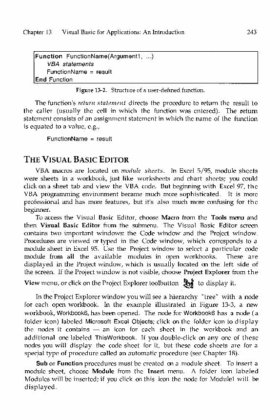
Chapter 13 Visual Basic for Applications: An Introduction 243
Function FunctionName(Argument1, . ..) VBA statements FunctionName = result
End Function
Figure 13-2. Structure of a user-defined function.
The function’s return statement directs the procedure to return the result to the caller (usually the cell in which the function was entered). The return statement consists of an assignment statement in which the name of the function is equated to a value, e.g.,
FunctionName = result
THE VISUAL BASIC EDITOR VBA macros are located on module sheets. In Excel 5/95, module sheets
were sheets in a workbook, just like worksheets and chart sheets; you could click on a sheet tab and view the VBA code. But beginning with Excel 97, the VBA programming environment became much more sophisticated. It is more professional and has more features, but it’s also much more confusing for the beginner.
To access the Visual Basic Editor, choose Macro from the Tools menu and then Visual Basic Editor from the submenu. The Visual Basic Editor screen contains two important windows: the Code window and the Project window. Procedures are viewed or typed in the Code window, which corresponds to a module sheet in Excel 95. Use the Project window to select a particular code module from all the available modules in open workbooks. These are displayed in the Project window, which is usually located on the left side of the screen. If the Project window is not visible, choose Project Explorer from the
View menu, or click on the Project Explorer toolbutton to display it.
In the Project Explorer window you will see a hierarchy “tree” with a node for each open workbook. In the example illustrated in Figure 13-3, a new workbook, Workbook6, has been opened. The node for Workbook6 has a node (a folder icon) labeled Microsoft Excel Objects; click on the folder icon to display the nodes it contains - an icon for each sheet in the workbook and an additional one labeled ThisWorkbook. If you double-click on any one of these nodes you will display the code sheet for it, but these code sheets are for a special type of procedure called an automatic procedure (see Chapter 18).
Sub or Function procedures must be created on a module sheet. To insert a module sheet, choose Module from the Insert menu. A folder icon labeled Modules will be inserted; if you click on this icon the node for Module1 will be displayed.

244 Excel for Chemists
Figure 13-3. The Visual Basic Editor’s Project Explorer window.
Figure 13-4. The Visual Basic Editor’s Properties window.

Chapter 13 Visual Basic for Applications: An Introduction 245
To change the name of the module from Module1 to a more descriptive one, choose Properties Window from the View menu, or click on the Properties Window toolbutton. In the Properties Window (Figure 13-4), highlight the name Module1 and type the new name.
GETTINGSTARTED:USINGTHERECORDER TOCREATEASUBPROCEDURE
Excel provides the Recorder, a useful tool for creating command macros. When you choose Macro from the Tools menu and Record New Macro... from the submenu, all subsequent menu and keyboard actions will be recorded until you press the Stop Macro button or choose Stop Recording from the Macro submenu. The Recorder is sufficient for creating simple macros, but you can’t use it to incorporate logic, branching or looping. After using the Recorder to create some simple macros, you’ll view it as simply a tool to create fragments of macro code for incorporation into more complex macros. Macros that involve only the use of menu or keyboard commands can be created using the Recorder.
The Recorder creates Visual Basic commands. You don’t have to know anything about Visual Basic to record a command macro in Visual Basic. This provides a good way to gain some initial familiarity with Visual Basic.
To illustrate the use of the Recorder, we’ll record the action of applying scientific number formatting to a number in a cell. First, select a cell in a worksheet and enter a number. Now choose Macro from the Tools menu, then Record New Macro... from the submenu. The Record Macro dialog box (Figure 13-5) will be displayed.
The Record Macro dialog box displays the default name that Excel has assigned to this macro: Macrol, Macro2, etc. Change the name in the Macro Name box to ScientificFormat (no spaces are allowed in a name). The “Store
Figure 13-5. The Record Macro dialog box.

246 Excel for Chemists
Macro In” box should display This Workbook; if not, choose This Workbook. Enter “e” in the box for the shortcut key, then press OK. The Macro Stop toolbar will appear (Figure 13-6), indicating that a macro is being recorded. If the Macro Stop toolbar doesn’t appear, you can always stop recording by using the Tools menu: in the Macro submenu the Record New Macro... command will be replaced by Stop Recording.
Figure 13-6. The Macro Stop toolbar.
Now choose Cells... from the Format menu, choose the Number tab and choose Scientific number format, then press OK. Finally, press the Macro Stop button.
To examine the macro code that you have just recorded, choose Macro from the Tools menu and Visual Basic Editor from the submenu. Click on the node for the module in the active workbook. This will display the code module sheet containing the Visual Basic code. The macro should look like the example shown in Figure 13-7.
Sub ScientificFormat()
’ Macro1 Macro ’ Macro recorded 7/12/2000 by E. J. Bill0
Selection.NumberFormat = “O.OOE+OO”
End Sub
Figure 13-7. Macro for scientific number-formatting, recorded in VBA.
This macro consists of a single line of code. You’ll learn about Visual Basic code in the chapters that follow.
To run the macro, enter a number in a cell, select the cell, then press the shortcut key combination that you designated when you recorded the macro. The number should be displayed in the cell in scientific format.
Excel Tip. If you have trouble locating the code module containing your macro, here’s what to do “when all else fails”: choose Macro from the Tools menu and Macros . . . from the submenu. Highlight the name of the macro in the Macro Name list box, and press the Edit button. This will display the code module sheet containing the Visual Basic code.

Chapter 13 Visual Basic for Applications: An Introduction 247
THE PERSONAL MACRO WORKBOOK
The Record Macro dialog box allows you to choose where the recorded macro will be stored. There are three possibilities in the “Store Macro In” list box: This Workbook, New Workbook and Personal Macro Workbook. The Personal Macro Workbook (PERSONAL.XLS in Excel for Windows, or Personal Macro Workbook in Excel for the Macintosh) is a workbook that is automatically opened when you start Excel. Since only macros in open workbooks are available for use, the Personal Macro Workbook is the ideal location for macros that you want to have available all the time.
Normally the Personal Macro Workbook is hidden (choose Unhide... from the Window menu to view it). If you don’t yet have a Personal Macro Workbook, you can create one by recording a macro as described earlier, choosing Personal Macro Workbook from the “Store Macro In” list box.
RUNNING A SUB PROCEDURE
In the preceding example, the macro was run by using a shortcut key. There are a number of other ways to run a macro. One of the most common is to use the Macro dialog box. Again, enter a number in a cell, select the cell, then choose Macro from the Tools menu and Macros... from the submenu. The Macro dialog box will be displayed (Figure 13-8). This dialog box lists all macros in open workbooks. To run the macro, select it from the list, then press the Run button.
Figure 13-B. The Macro dialog box.

248 Excel for Chemists
Here are some (but not all) of the ways to run a command macro:
from the Macro dialog box, as described in this chapter
l by means of a shortcut key, as described in this chapter
l by means of a custom menu command, as described in Chapter 18
by means of a custom button on a toolbar, as described in Chapter 19
by means of a button on a worksheet, as described in Chapter 8 0 as a subroutine called by another macro, as described in Chapter 15
l by means of an automatic procedure (Excel 5/95) or event-handler procedure (Excel 97) , as described in Chapter 18
ASSIGNING A SHORTCUT KEY
TO A SUB PROCEDURE
If you didn’t assign a shortcut key to the macro when you recorded it, but would like to do so “after the fact”, choose Macro from the Tools menu and Macros... from the submenu. Highlight the name of the macro in the Macro Name list box, and press the Options... button. You can now enter a letter for the shortcut key: CONTROL+(key) or SHIFT+CONTROL+(key) in Excel for Windows, OPTION+COMMAND+(key) or SHIFT+OPTION+COMMAND+(key) in Excel for the Macintosh.
GETTING STARTED: CREATING A SIMPLE CUSTOM FUNCTION
As a simple first example of a Function procedure, we’ll create a custom function to convert temperatures in degrees Fahrenheit to degrees Celsius.
Fu net ion procedures can’t be recorded; you must type them on a module sheet. You can have several macros on the same module sheet, so if you recorded the ScientificFormat macro earlier in this chapter, you can type this custom function procedure on the same module sheet. If you do not have a module sheet available, insert one by choosing Module from the Insert menu.
Type the macro as shown in Figure 13-9. DegF is the argument passed by the function from the worksheet to the module (the Fahrenheit temperature); the single line of VBA code evaluates the Celsius temperature and returns the result to the caller (in this case, the worksheet cell in which the function is entered).
Function FtoC(DegF) FtoC = (DegF - 32) * 5 / 9
End Function Figure 13-9. Fahrenheit to Celsius custom function.

Chapter 13 Visual Basic for Applications: An Introduction 249
USING A FUNCTION MACRO
A custom function is used in a worksheet formula in exactly the same way as any of Excel’s built-in functions. You can enter it in a formula by using Paste Function, or by typing it. The workbook containing the custom function must be open.
Touse Paste Function, follow the procedure described in Chapter 3. Select the worksheet cell or the point in a worksheet formula where you want to enter the function (e.g., cell 82 in Figure 13-10). Choose Function... from the Insert
menu or press the Paste Function toolbutton j$m to display the Paste Function dialog box. Scroll through the Function Category list and select the User Defined category. The FtoC function will appear in the Paste Function list box. When you press OK, the Formula Palette (the Paste Function Step 2 of 2 dialog box) will be displayed. Enter the argument, or click on the cell containing the argument to enter the reference (cell A2 in Figure 13-lo), then press the OK button.
Figure 13-10. A custom function.
You can also type the function name, with or without the opening parenthesis, and then press CONTROL+A or CONTROL+SHIFT+A, as described in Chapter 3. The function placeholder argument will be displayed, highlighted so that you can enter a value or reference (Figure 13-11).
Figure 13-11. Entering a custom function by using CONTROL+SHIFT+A.
Unfortunately, if you’re entering the custom function in a different workbook than the one that contains the custom function, the function name must be entered as an external reference, e.g. PERSONAL.XLS!FtoC. This can make typing the function rather cumbersome, and means that you’ll probably enter the function by using Excel’s Paste Function. But, see “Creating Add-In Function Macros” in Chapter 17 for a solution to the problem.

250 Excel for Chemists
RENAMING A MACRO To rename a Sub procedure, access the Visual Basic Editor and click on the
module containing the macro. The name of the macro is in the first line of code, immediately following the Sub keyword. Simply edit the name.
How Do I SAVE A MACRO? A macro is part of a workbook, just like a worksheet or a chart. To save the
macro, you simply Save the workbook.

14 PROGRAMMING WITH VBA
This chapter provides an overview of macro programming using VBA. If you are familiar with programming in other versions of BASIC or in FORTRAN, many of the programming techniques described in this chapter will be familiar.
CREATING VISUAL BASIC CODE VBA has a wide range of commands, functions and methods that can be used
to create custom applications, and this tends to make VBA confusing for the beginner (or even the non-beginner). This chapter covers the basics that you will need to get started.
ENTERING VBA CODE
use When you type VBA . code in a module, it’s TAB to indent related lines for easier reading.
good programming practice to
As you type your VBA code, Excel checks each line for errors. A line that contains one or more errors will be displayed in red, or another color if previously specified. Variables usually appear in black. Other colors are also used: comments (see later) are usually green and VBA keywords (Fu net i o n , Range, etc.) usually appear in blue.
You can enter numbers in E format but they will automatically be converted to floating point. You can’t enter numbers as percentages; the percent symbol has another meaning in VBA (see “VBA Data Formats” later in this chapter).
If you type a long VBA expression, it will not wrap to the next line but will simply disappear off the screen. You will have to insert a line-continuation character (a space followed by the underscore character followed by RETURN) to cause a line break in a line of VBA code, as in the following example:
ReturnValu = InputBox(“Enter validation code number”, -
“Validation of this copy of SOLVER.STATS”)
The line-continuation character can’t be used within a string.
Several VBA statements can be combined in one line by separating them with colons. For example, the procedure in Figure 14-1 can be replaced by the more compact one in Figure 14-2 or even by the one in Figure 14-3.
251
Excel for Chemists: A Comprehensive Guide. E. Joseph BilloCopyright 2001 by John Wiley & Sons, Inc.
ISBNs: 0-471-39462-9 (Paperback); 0-471-22058-2 (Electronic)

252 Excel for Chemists
Sub MultiBeeper For x = ITo 10 Beep Next End Sub
Figure 14-l. A simple VBA Sub procedure.
Sub MultiBeeper For x = 1 To 10: Beep: Next End Sub
Figure 14-2. A Sub procedure with several statements combined.
Sub MultiBeeper : For x = 1 To 10: Beep: Next : End Sub
Figure 14-3. A Sub procedure in one line.
MAKING A REFERENCE TO A CELL OR RANGE OF CELLS
One of the most important things you’ll need to master is the technique of making a reference to a cell or range of cells. In brief, you’ll need to be able to send values from a worksheet to a module sheet so that you can perform operations on the worksheet data, and you’ll need to be able to send the results back from the module sheet to the worksheet.
You can reference a particular cell or range within a worksheet in a number of ways: by selecting a cell or range by using the Select keyword, by using the Selection or ActiveCell keywords, or by using the Range method or the Cells method.
Don’t use the Select keyword unless you actually need to select cells in a worksheet. For example, to copy a range of cells from one worksheet to another, you could use the statements shown in Figure 14-4, and in fact this is exactly the code you would generate using the Recorder. But you can do the same thing much more efficiently, and without switching from one worksheet to another, by using the code shown in Figure 14-5.
Range(“D1 :D2O”).Select Selection.Copy Sheets(“Sheetl!Y’).Select Range(“A1 “).Select ActiveSheet.Paste
Figure 14-4. VBA code fragment by the Recorder.
, Range(“p1 :D20”).Copy (Sheets(“Sheet1 V’).Range(“Al ‘I))
Figure 14-5. A more efficient way to accomplish the same thing, without selecting cells.

Chapter 14 Programming with VBA 253
MAKING A REFERENCE TO THE ACTIVE CELL
OR A SELECTED RANGE OF CELLS
You may wish to create a macro that operates on the contents of a user- selected cell or range. To do this you can use either the ActiveCell keyword or the Selection keyword.
Note the difference between the active cell and the selection: Selection can be a range of cells or a single cell; ActiveCell (always a single cell) refers to the cell in the upper-left corner of a range if applied to a range of cells.
MAKING A REFERENCE TO A CELL OTHER THAN THE ACTIVE CELL
Instead of a macro that gets the contents of the active cell or a selection, you may want to create a macro that copies values from specified rows and columns in a worksheet, independent of where the cursor has been “parked” by the user. To accomplish this, you can use either the Range method or the Cells method to make a reference to a cell or range. The syntax of the Cells method is Cells(mv, column). The first two of the following refer to cell 83, the next two to the range B3:E27.
Range(“B3”)
Cells(3,2)
Range(“B3:E27”)
Range(Cells(3, 2), Cells(27, 5))
The preceding examples are “absolute” references, since they always refer to B3 or B3:E27. You can also use what could be called a “computed” reference, in which the reference depends on the value of a variable. The Cells method is conveniently used in this way. For example, the expression
Cells(x,2)
allows you to select any cell in column B, depending on the value assigned to the variable x. The Range method can be used in a similar way by using the concatenation operator, e.g.,
Range(“B” & x)
REFERENCES USING THE UNION OR INTERSECT METHOD
VBA can create references by using methods that are the equivalents of the union operator or intersection operator described in Chapter 3. The Union method creates a reference that includes multiple selections, e.g., Al ,B5 or G3:L3,G5:L5. The syntax of the Union method is Union(range1, range2). The Intersect method creates a reference that is common to two references (e.g.,

254 Excel for Chemists
F4:F6 E5:15). The syntax of the Intersect method is Intersect(range1, range2). Both range7 and range2 must be Range objects.
GETTING VALUES FROM A WORKSHEET
To transfer values from worksheet cells to a procedure, use a reference to a worksheet range in an assignment statement, like the following.
variable1 = ActiveCelLValue
QZ = Worksheets(“Sheet1 “).Range(“AS”).Value
The Value keyword can usually be omitted:
MyVal = Range(“A” & x)
CellVal = Cells(StartRow+x,StartCol)
The corresponding rather than its value.
Form u I a property is used to obtain the formula in a cell,
SENDING VALUES TO A WORKSHEET
To send values from a module sheet back to a worksheet, simply use an assignment statement like the following. Numbers, text, the contents of a VBA variable, even a worksheet formula can be entered into worksheet cells or ranges.
Cells(1, 2).Value = 5
Range(“E1 “).Value = “Jan.-Mar.”
Worksheets(“Sheet1 “).Range(“Al”) = variable2
Cells(1, 3) = ” =sum(Fl:FlO)”
CREATING VISUAL BASIC CODE: COMPONENTS OF VISUAL BASIC STATEMENTS
VBA macro code consists of statements. Statements are constructed by using VBA commands, operators, variables, functions, objects, properties or methods. (VBA Help refers to keywords such as Beep, Do or Exit as statements, but here they’ll be referred to as commands, and we’ll use “statement” in a general way to refer to a line of VBA code.)
OPERATORS
VBA operators include the arithmetic operators (+, -, *, /, *), the text concatenation operator (&), the comparison operators (=, c, >, c=, >=, o) and the Boolean or logical operators, which are discussed later.

Chapter 14 Programming with VBA 255
Excel Tip. Be sure to leave a space on either side of the concatenation operator; otherwise it will be mistaken for a type-declaration character (see “VBA Data Types ” later in this chapter).
VARIABLES AND ARGUMENTS
or Variables
references. are the names you create to indicate the storage locations of values
Arguments are variables that are passed from a worksheet to a procedure, for example.
The value of a variable is determined by an assignment statement. An assignment statement assigns the result of an expression to a variable or object; the form of an assignment statement is:
variable = expression
In an Excel worksheet, you have to use Define Name or Create Name to assign a name to a variable, but variable names in VBA a re automatica .llY assigned as you type the VBA code in a module. There are just a few rules for naming variables or arguments:
l You can’t use any of the VBA reserved words, such as Function, Range or Value.
l The first character must be a letter.
l A name cannot contain a space or a period.
l The type-declaration characters (%, $, #, !, &) cannot be embedded in a name.
You can use either upper- or lowercase letters. If you change the case of a variable name in the line you are currently typing (e.g., from variable1 to Variablel), VBA will change all instances of the old form of the variable to the new form.
You should make variable names as descriptive as possible, but avoid overly long names which are tedious to type. You can use the underscore character to indicate a space between words (e.g., formula-string). Don’t use a period to indicate a space, since VBA reserves the period character for use with objects. The most popular form for variable names uses upper- and lowercase letters (e.g., FormulaString).
OBJECTS,PROPERTIESANDMETHODS VBA is an object-oriented programming language. Objects in Microsoft Excel
are the familiar components of Excel, such as a worksheet, a chart, a toolbar or a range. Objects have properties and methods associated with them. Objects are the nouns of the language, properties are the adjectives, and methods are the verbs.

256 Excel for Chemists
OBJECTS
Some examples of VBA objects are the Workbook object, the Worksheet object, the Chart object and the Range object. A complete list of objects in Microsoft Excel is listed in Excel’s On-line Help. You can also use the Object Browser to see the complete list of objects. To display the Object Browser dialog box, choose Object Browser from the View menu.
There is a hierarchy of objects. You specify the object by specifying its location in a hierarchy, separated by periods, e.g.,
Workbooks(“Book1 “).Worksheets(“Sheet3”).Range(“E!Y’)
Figure 14-6 shows an abbreviated hierarchical list of the most useful objects.
You can also refer to collections of objects. A collection is a group of objects of the same kind. A collection has the plural form of the object’s name (e.g., Worksheets). Worksheets refers to all worksheets in a particular workbook. To reference a particular worksheet, you use the reference Worksheets(NameText); for example, Worksheets(“Spectrum1 ‘I).
To distinguish a particular collection of worksheets in a particular workbook, use the period operator to connect object names. For example, to refer to the Worksheet Spectrum1 in the Workbook Deconvolution, use the reference Workbooks(“Deconvolution”).Worksheets(”Spectruml ‘I). To refer to a particular cell within the worksheet, use
Workbooks(“DeconvoIution”).Worksheets(”Spectruml “).Range(“ES”)
If Deconvolution is the only open workbook, and Spectrum1 is the active sheet, you can omit references to them and simplv use the reference Range(“E5”).
Application MenuBar Menu Menultem
ToolBar ToolbarButton
Workbook Chart Axis AxisTitle
GridLines
TickLabels
etc.
Worksheet PageSetup
Range Areas
etc.
Figure’14-6. Partial list of objects, arranged in hierarchical order.

Chapter 14 Programming with VBA 257
SOME USEFUL OBJECTS
The objects you probably will use most often in the beginning are the Workbook object, the Worksheet object and the Range object. (For reasons that will become clear in a while, there is no Cell object.) Later you may use the Dialog, MenuBar, ToolBar or Chart objects and the objects they in turn contain.
“OBJECTS” THAT ARE REALLY PROPERTIES
Although ActiveCell and Selection are properties, not objects, you can treat them like objects. (ActiveCell is a property of the Application object, or the ActiveWindow property of the Application object.) The Application object has the following properties that you can treat just as though they were objects: the ActiveWindow, ActiveWorkbook, ActiveSheet, ActiveCell, Selection and ThisWorkbook properties. Since there is only one Application object, you can omit the reference to Application and simply use ActiveCell.
YOU CAN DEFINE YOUR OWN OBJECTS
VBA allows you to equate a variable to an object, but the variable does not automatically become an object. If you then attempt to use the variable in an expression that requires an object, you’ll get an “Object required” error message. The Set command lets you define a variable or property as an object. The following example makes the InputBox method return an Object (so that you can use its Address property in addition to its Value property, for example):
Set known Ys = Application.lnputBox (“Select the-range of Y values”, “STEP 1 OF 2”, , , , , , 8)
PROPERTIES
Objects have properties that can be set or read. Some properties of the Range object are the ColumnWidth property, the NumberFormat property, the Font property, the Value property. A property is connected to the object it modifies by a period, e.g.,
CelFmt = Range(“ES”).NumberFormat
returns the number formatting of cell E5 and assigns it to the variable CelFmt, and
Range(“E5”). NumberFormat = “0.000”
sets the number formatting of cell E5. (Some properties, such as Column or Count, are read-only.)
Properties can also modify properties.

258 Excel for Chemists
SOME USEFUL PROPERTIES
There is a large and confusing number of properties: VBA Help lists a total of 486 property names. The list of properties belonging to the Range object alone contains more than 40 entries. Some of the most useful properties of the Range object are listed in Table 14-1.
Table 14-l. Some Useful VBA Pronerties
Column
ColumnWidth Count Font Formula Name NumberFormat Row
RowHeight Text Value
Returns a number corresponding to the first column in the range. Returns or sets the width of all columns in the range. Returns the number of items in the range. Returns or sets the font of the range. Returns or sets the formula. Returns or sets the name of the range. Returns or sets the format code for the range. Returns a number corresponding to the first row in the range. Returns or sets the height of all rows in the range. Returns or sets the text displayed by the cell. Returns or sets the contents of the cell or range.
USING PROPERTIES
In a VBA macro, many times you’ll need to determine the value or state of an object’s property, or change it. There are two kinds of property: read-only and read-write. Properties can have values that are numeric, string or logical.
To return an object’s property, use the following syntax:
VariableName = ObjectName. PropertyName
To set an object’s property (only if it is a read-write property, of course), use the following syntax:
ObjectName. PropertyName = expression
For example, to change the background color of a range of cells to blue, use the statement
Range(“A5:ES’).Interior.Colorlndex = 8
METHODS
Objects also have methods. Methods can operate on an object or on a property of an object. Some methods that can be applied to the Range object are the

Chapter 14 Programming with VBA 259
Copy method, the Cut method, the FillDown method or the Sort method. For example,
Range(“A1 :El “).Clear
clears the formulas and formatting in the range Al : E 1.
SOME USEFUL METHODS
VBA Help lists 267 methods. Many of them correspond to familiar menu commands. For example, Copy, C u t , C I ea r and Sort can be performed on a range of cells. Some useful VBA methods are listed in Table 14-2.
Table 14-2. Some Useful VBA Methods Activate Activates an object (sheet, etc.). Clear Clears an entire range. Close Closes an object.
COPY Copies an object to a specified range or to the Clipboard. cut Cuts an object to a specified range or to the Clipboard. FillDown Copies the cell(s) in the top row into the rest of the range. Select Selects an object.
TWO WAYS TO SPECIFY ARGUMENTS
VBA methods usually take one or more arguments. The Sort method, for example, takes 10 arguments. The syntax of the Sort method is
object.Sort(keyl, orderl, key2, order2, key3, order3, header, orderCustom, ma tchcase, orientation)
The object argument is required; all other arguments are optional.
You can specify the arguments of a method in two ways. One way is to list the arguments in order as they are specified in the preceding syntax, i.e.,
Selection.Sort Range(“A2”), 1
(In the preceding example, only the arguments key1 and order1 were specified; the remaining arguments are optional and were not required.)
The second way is to use the name of the argument as it appears in the preceding syntax, with the := operator, to specify the value of the argument. The arguments can appear in any order, as in the following (all in one line of code, of course):
Selection.Sort Key1 :=Range(“A2”), Order1 :=xlAscending, Key2:=Range(“B2”), Order2:=xlAscending, Key3:=Range(“C2”), Order3:=xIDescending, Header :=xlGuess, OrderCustom:=l, MatchCase:=False, Orientation:=xlTopToBottom

260 Excel for Chemists
ARGUMENTS WITH OR WITHOUT PARENTHESES
As well as performing an action, methods create a return value. The return value can be either True or False. Even the ChartWizard method creates a return value: True if the chart was created successfully, False if the method failed. Usually you aren’t interested in these return values.
An example of a method that creates a useful return value is the CheckSpelling method. The CheckSpelling method has the following v
syntax:
Application.CheckSpeIling(word)
If you use this method, you’ll need the return value (either True or False > determine whether the word is spelled correctly.
If you want to use the return value of a method, you must enclose
to
the arguments of the method in parentheses. If the arguments are not enclosed in parentheses, then the return value will not be available for use. Put another way, the expression
result = Application.CheckSpelling(ActiveCell.Value)
does not produce a syntax error, while the expression
result = ApplicationXheckSpelling ActiveCell.Value
does give a syntax error.
SOME USEFUL FUNCTIONS
The functions available in VBA are similar to the functions available in Excel itself. There are 108 VBA functions listed in VBA Help. Table 14-3 lists some of the more useful ones for numerical calculations.
USING WORKSHEET FUNCTIONS WITH VBA
Many useful worksheet functions do not have a VBA equivalent. To use them, use the syntax
Application.WorksheetFunction
and supply arguments for the function just as you would in a worksheet. For example, to use the FIND function in VBA, use the code
AppIication.Find(find_text,wifhin_text,start_num)
e-g=,
Application.Find(“]“,Range(“Al ‘I), 1)

Chapter 14 Programming with VBA 261
Table 14-3. Some Useful VBA Functions
Abs Returns the absolute value of a number. Asc Returns the character code of a character. Chr Returns the character corresponding to a code.
ExP Returns e raised to a power. Fix Returns the integer part of a number (truncates). Int Returns the integer part of a number (rounds down).
IsArray Returns True if the variable is an array.
IsNull Returns True if the expression is null (i.e., contains no valid data).
Is N u me r i c Returns True if the expression can be evaluated to a number.
LBound
LCase Left
Len
Log Mid Right RTrim
Sqr Str UBound
UCase
Returns the lower limit of an array dimension.
Converts a string into lowercase letters. Returns the leftmost characters of a string. Returns the length (number of characters) in a string.
Returns the natural (base-e) logarithm of a number.
Returns a specified number of characters from a string. Returns the rightmost characters of a string. Returns a string without trailing spaces. Returns the square root of a number.
Converts a number to a string. Returns the upper limit of an array dimension. Converts a string into uppercase letters.
SOME USEFUL VBA COMMANDS
Commands in VBA are similar to commands in BASIC or FORTRAN. Table 14-4 lists some of the most useful VBA commands.
VBA DATATYPES VBA uses a range of different data types. Table 14-5 lists the built-in data
types.
Unless you declare a variable’s type, VBA will use the Variant type. You can save memory space if your procedure deals only with integers, for example, by declaring the variable type.
You can also declare a variable’s type by appending a type-declaration character to the variable name, a technique from older versions of BASIC. The type-declaration characters include % for integer variables and $ for string variables.

262 Excel for Chemists
Table 14-4. Some Useful VBA Commands
Beep
Dim
Do...Loop
Else
Elself
End
End If
Exit
For Each...Next
For...Next
Function
GoSub...Return
GoTo
If...Then...Else
On...GoSub
On...GoTo
Select Case
Set
stop
Sub
Until
While
With...EndWith
Makes a “beep” sound.
Declares an array (see Chapter 15) and allocates storage for it.
Delineates a block of statements to be repeated.
Optional part of If...Then structure.
Optional part of If...Then structure.
Terminates a procedure.
Terminates block of statements begun by If.
Exits a Do..., For . . . . Function... or Sub... structure.
Delineates a block of statements to be repeated.
Delineates a block of statements to be repeated.
Marks the beginning of a Function procedure.
Delineates a subroutine.
Unconditional branch.
Delineates a block of conditional statements.
Branch to one of several specified subroutines.
Branch to one of several specified lines.
Executes one of several blocks of statements.
Assigns an object reference to a variable or property.
Stops execution.
Marks the beginning of a Sub procedure.
Optional part of Do...Loop structure.
Optional part of Do...Loop structure.
Delineates a block of statements to be executed on a single object.
THE VARIANT DATA TYPE
The Variant data type is the default data type in VBA. Like Excel itself, the Variant data type handles and interconverts between many different kinds of data: integer, floating point, string, etc. The Variant data type automatically chooses the most compact representation. But if your procedure deals with only one kind of data, it will be more efficient and usually faster to declare the variables as, for example, Integer.

Chapter 14 Programming with VBA
Table 14-5. VBA’s Built-in Data Tvnes 3 Data t e
Logical 2 bytes True or False
Integer 2 bytes -32,768 to 32,767
Long integer 4 bytes -2,147,483,648 to 2,147,483,647
263
Single precision 4 bytes
Double precision 8 bytes
-3.402823E38 to -1.401298E-45 for negative values; 1.401298E-45 to 3.402823E38 for positive values
-1.79769313486232E308 to 4.94065645841247E-324 for negative values; 4,94065645841247E-324 to 1.79769313486232E308 for positive values
Currency 8 bytes -922,337,203,685,477.5808 to 922,337,203,685,477.5807
Date
Object
String
Variant
8 bytes
4 bytes
1 byte/character
16 bytes + 1 byte/character
Any Object reference
Any numeric value up to the range of a Double or any text
STRING DATA TYPES
Strings can be stored either as variable-length strings (the default data type) or as fixed-length strings. To declare a string variable as fixed-length, use the statement in a Dim statement (more about the Dim statement in Chapter 15)
String * length
For example, the following statement sets aside storage for a two- dimensional array of names and addresses, containing fixed-length strings of 32 characters:
Dim AddressList(4,500) As String * 32
If a string of length less than 32 characters is assigned to the array AddressList, trailing spaces are added to fill out the string length. If a string of more than 32 characters is assigned to Addresslist, the string will be truncated.

264 Excel for Chemists
THE BOOLEAN (LOGICAL) DATA TYPE
A logical variable can have only the value True or True and Fal se are often implied; thus the expressions
False. The keywords
If (j > N) = True Then ALPHA = “n/a”
and
If (j > N) Then ALPHA = “n/a”
are equivalent.
You can use other data types as Boolean variables. When a variable is used in a logical expression, zero is converted to False while any non-zero value is converted to True. Thus the expression
If j Then expression
tests for a non-zero value of the variable j.
When Boolean variables are converted to other data types, False becomes zero but True is converted to -1.
DECLARING VARIABLES OR ARGUMENTS IN ADVANCE
VBA uses the Va r i a n t data type as the default data type for variables and arguments. The Variant data type permits Excel to switch between floating- point, integer and string variables as required.
You can force a particular variable or argument to take a specified data type. For variables, use the Dim statement, e.g.,
Dim ChemFormula As String
SPECIFYING THE DATA TYPE OF AN ARGUMENT
You can specify the data type of an argument passed to a Function procedure by using the As keyword in the Function statement. For example, if the Fun ction procedure MO decimals (an integer), then the
IWt has two arguments, formula (a string) and statement
Function MolWt (formula As String, decimals As Integer)
declares the type of each variable. If an argument of an incorrect type is supplied to the function, a #VALUE! error message will be displayed.
SPECIFYING THE DATA TYPE RETURNED BY A FUNCTION PROCEDURE
You can also specify the data type of the return value. If none is specified, the Variant data type will be returned. In the example of the preceding section, MolWt returns a floating-point result. The Variant data type is satisfactory;

Chapter 14 Programming with VBA 265
however, if you wanted to specify double precision floating-point, use an additional As Type expression in the statement, e.g.,
Function MolWt (formula As String, decimals As Integer) As Double
PROGRAMCONTROL If you are familiar with computer languages such as BASIC or FORTRAN,
you will find yourself quite comfortable with most of the material in this section.
DECISION-MAKING (BRANCHING)
VBA supports If... Then and If...Then...Else or Elself structures, very similar to the Excel worksheet function IF. In addition, VBA provides the Select Case decision structure, similar to the ON value GOT0 statement in BASIC.
The If...Then statement can be on a single line: If (x = j) Then numerator = 10 * (logbeta - pH * x)
or it can be followed by multiple statement lines as in Figure 14-7, (the Block If statement).
If (pKa logical log beta
= False) Then = logbeta + pKs_or-logKs(x)
denom = denom + 10 * (logbeta - pH * x) etc.
End If
Figure 14-7. Example of VBA If...End If structure.
If...Then...Else or Elself structures are also possible. For example:
If LogicalExpression Then statement Else statement
or, as illustrated in Figure 14-8, you can employ several logical expressions.
If LogicalExpression Then statements
Elself LogicalExpression Then statements
Elself LogicalExpression Then statements etc.
End If
Figure 14-B. The VBA If...Elself...End If structure.

266 Excel for Chemists
The Select Case statement provides an efficient alternative to the series of Elself conditionN statements when conditionN is a single expression that can take various values. The syntax of the Select Case statement is illustrated in Figure 14-9.
TestExpression is evaluated and used to direct program flow to the appropriate Case. ExpressionListN can be a single value, a list of values separated by commas or a range of values. The optional Case Else statement is executed if TestExpression doesn’t match any of the values in any of Expression List N.
The example shown in Figure 14-10 illustrates the use of Select Case to calculate the pKa value of a polyprotic acid. Since data at or near the equivalence points cause large calculation errors, the pKa is calculated only for n-bar values in the range 0.2 - 0.8, 1.2 - 1.8, 2.2 - 2.8 or 3.2 - 3.8. The expression used to calculate the pKa from the n-bar parameter depends on the number of protons
bound, i.e., on the value of n-bar. The Select Case statement is used to direct program flow to the appropriate expression.
Note that a range of values is indicated by using the To keyword.
Select Case TestExpression Case Expression List 1 statements Case ExpressionList statements Case ExpressionList statements Case Else statements
End Select
Figure 14-9. The VBA Select Case structure.
LOGICAL OPERATORS l 1 You are already familiar with the And and Or operators, but VBA provraes
in addition the Xor (exclusive or) operator. The operators have the following syntax:
expression 1 And expression2 T r u e if both expressions are Tr u e .
expression 1 Or expression2 True if either expression is True.
expression1 Xor expression2 True if one expression is True, the other False.

Chapter 14 Programming with VBA
NBar=(ZP*CR+CA+COH-CH-CNa)/CR
Select Case NBar Case 3.2 To 3.8
pK = pH + Application.Log((NBar - 3) / (4 - NBar)) Case 2.2 To 2.8
pK = pH + Application.Log((NBar - 2) / (3 - NBar)) Case 1.2 To 1.8
pK = pH + Application.Log((NBar - 1) / (2 - NBar)) Case 0.2 To 0.8
pK = pH + Application.Log((NBar) / (1 - NBar)) Case Else
PK = II II
End Select
End Sub
267
Figure 14-10. An example of the Select Case structure.
The preceding expressions must evaluate to True or False; that is, they must be logical expressions. The logical operators are almost always used in combination with If statements.
More than one And or Or can be combined in a single statement. For example
If Char = II ” Or Char = II*” Or Char = ‘I,” Or Char = I’(” 0 r Char = ‘1/11 T h e n . . .
evaluates to True if any one of the logical expressions is T r u e .
Parentheses are often necessary to control the logic of the expression. For example, each of the expressions
If (expression1 And expression2) Or expression3 Then . . .
If expression1 And (expression2 Or expression3) Then...
has eight different possible combinations of expressionl, expression2 and expression3; two of them give different outcomes depending on which expression is used.
LOOPING The loop structures in VBA are similar to those available in other
programming languages.

268 Excel for Chemists
FOR...NEXT LOOPS
The syntax of the For...Next loop is given in Figure 14-11.
For Counter = Start To End Step Increment statements
Next Counter
Figure 14-U. The VBA For...Next structure.
Both Step Increment in the For statement, and Counter following the N ex t are optional. If Increment is omitted, it is set equal to 1. Increment can be negative.
FOR EACH...NEXT LOOPS
The For Each...Next loop structure is similar to the For...Next loop structure, except that it executes the statements within the loop for each object within a group of objects. Figure 14-12 illustrates the syntax of the statement.
For Each Element In Group statements
Next Element
Figure 14-12. The VBA For Each...ln...Next structure.
An important point: the For..Each . ..Next loop returns an object variable in each pass through the loop. You can access or use all of the properties or methods that apply to Element. For example, in a loop such as
For Each ccl In Selection
the variable ccl is an object that has all the properties of a cell (a Range object): Value, Formula, NumberFormat, etc.
DO WHILE... LOOP
The Do While...Loop is used when you don’t know beforehand how many times the loop will need to be executed. The syntax is shown in Figure 14-13.
Do While LogicalExpression statements
LOOP
Figure 14-13. The VBA DO While...Loop structure.
Do statements
LOOD While LoaicalExDression
Figure 14-14. Alternate form of DO While...Loop structure.

Chapter 14 Programming with VBA 269
An alternate format of this type of loop places While LogicalExpression at the end of the loop, as exemplified in Figure 14-14.
Note that this form of the Do While structure executes the loop at least once.
EXITING FROM A LOOP OR FROM A PROCEDURE
Often you use a loop structure to search through an array or collection of objects, looking for a certain value or property. Once you find a match, you don’t need to cycle through the rest of the loops. You can exit from the loop using the Exit For (from a For...Next loop or For Each...Next loop) or Exit Do (from a Do While... loop). The Exit statement will normally be located within an If statement. For example,
If CellContents.Value c= 0 Then Exit For
Use the Exit Sub or Exit Function to exit from a procedure. Again, the Exit statement will normally be located within an If statement.
Exit statements can appear as many times as needed within a procedure.
SUBROUTINES Although all Sub procedures are subroutines, by “subroutine” we mean a
subprogram that is called by another VBA program. It’s good programming practice to break up a complicated task into simpler tasks and write subroutines to do each task. The separate subroutines are called by a main program.
There are several ways to execute a subroutine within a main program. The two most common are by using the Call command, or by using the name of the subroutine. These are illustrated in Figure 14-15. MainProgram calls subroutines Task1 and Task2, each of which requires arguments.
Sub MainProgram etc. Call Task1 (argument1 ,argument2) etc Task2 argument3,argument4 etc End Sub
Sub Task1 (ArgNamel ,ArgName2) etc End Sub
Sub Task2(ArgName3,ArgName4) etc End Sub
Figure 14-15. A main program illustrating the different syntax of subroutine calls.

270 Excel for Chemists
The two methods use different syntax if the subroutine requires arguments. If the Call command is used, the arguments must be enclosed in parentheses. If only the subroutine name is used, the parentheses must be omitted. Note that the variable names of the arguments in the calling statement and in the subroutine do not have to be the same.
SCOPING A SUBROUTINE
A subroutine can be Public or Private. Public subroutines can be called by any subroutine in any module. The default for any Sub procedure is Public. A Private subroutine can be called only by other subroutines in the same module. To declare the subroutine Task3 as a private subroutine, use the statement
Private Sub Task30
INTERACTIVEMACR~S VBA provides two built-in dialog boxes for display of messages or for input,
MsgBox and InputBox.
MSGBOX
The Msg Box dialog box allows you to display a message, such as “Please wait...” or “Access denied”. The box can display one of three message icons, and there are many possibilities in the number and function of buttons that can be displayed.
The syntax of MsgBox is
Msg Box (prompt text, - buttons, title text, - helpfile, context)
where prompt- text is the message displayed within the box, buttons specifies the buttons to be displayed and tit/e text is the title to be displayed in the Title - Bar of the box. For information about helpfile and context, refer to Microsoft Excel Visual Basic Reference.
For example, the VBA expression
MsgBox “You entered ” & incr & ‘7’ & Chr(13) & Chr(13) & _
“That value is too large.” & Chr(13) & Chr(13) & “Please try again.“, 64
produces the message box shown in Figure 14-16.
The value of buttons determines the type of message icon and the number and type of response buttons; it also determines which button is the default button. The possible values are listed in Table 14-6. The values of buttons are built-in constants - for example, the value 64 for buttons can be replaced by the

Chapter 14 Programming with VBA 271
Figure 14-16. A Msgbox display.
variable name vblnformation. (For a complete list of names of these built-in constants, refer to Microsoft Excel Visual Basic Reference.) The values 0 - 5 specify the number and type of buttons, values 16 - 64 specify the type of message icon, and values 0, 256, 512 specify which button is the default button. You can add together one number from each group to form a value for buttons. For example, to specify a dialog box with a Warning Query icon, with Yes, No and Cancel buttons, and with the No button as default, the values 32 + 3 + 256 = 291. The same result can be obtained by using the expression
buttons = vblnformation + vbYesNoCancel + vbDefaultButton2
and using the variable buttons in the MsgBox function.
Table 14-6. Values for the buttons Parameter of M sg Box
buttons Description Display OK button only. Display OK and Cancel buttons. Display Abort, Retry and Ignore buttons. Display Yes, No and Cancel buttons. Display Yes and No buttons. Display Retry and Cancel buttons.
16 Display Critical Message icon. 32 Display Warning Query icon. 48 Display Warning Message icon. 64 Display Information Message icon
0 First button is default. 256 Second button is default. 512 Third button is default.

272 Excel for Chemists
MSGBOX RETURN VALUES
MsgBox returns a value that indicates which button was pressed. This allows you to take different actions depending on whether the user pressed the Yes, No or Cancel buttons, for example. To get the return value of the Message Box, use an expression like
RtnValu = MsgBox (prompt text, - buttons, title text, - helpfile, context)
The return values of the buttons are as follows: OK, 1; Cancel, 2; Abort, 3; Retry, 4; Ignore, 5; Yes, 6; No, 7.
INPUTBOX
The InputBox allows you to pause a macro and request input from the user. There are both an InputBox Function and an InputBox method.
The syntax of the InputBox Function is
InputBox(prompt text, - tit/e text, - default, x-position, y-position, helpfile, context)
where prompt-text and tit/e-text are as in MsgBox. Default is the expression displayed in the input box, as a string. The horizontal distance of the left edge of the box from the left edge of the screen, and the vertical distance of the top edge from the top of the screen are specified by x - position and y position, - respectively. For information about helpFile and context, refer to Microsoft Excel Visual Basic Reference.
If the user presses the OK button or the RETURN key, the Input Box function returns as a value whatever is in the text box. If the Cancel button is pressed, the function returns a null string. The following example produces the input box shown in Figure 14-17.
ReturnValu = InputBox(“Enter validation code number”, - “Validation of this copy of SOLVER.STATS”)
Figure 14-17. An InputBox display.

Chapter 14 Programming with VBA 273
The syntax of the InputBox method is
0 bject.lnputBox (prompt text, tit/e-text, default, x-position, y-position, helpfile, context, type-num)
The differences between the InputBox function and the InputBox method are the following: (i) default can be any data type and (ii) the additional argument type-num specifies the data type of the return value. The values of type - num and the corresponding data types are listed in Table 14-7. Values of type num can be added together. For example, to specify an input dialog box that would accept number or string values as input, use the value 1 + 2 = 3 for type num. -
Table 14-7. ImutBox Data Tvne Values
type num - 0 1 2 4 8 16 64
Data type Formula Number String Logical Reference (as a Range object) Error value Arrav
TESTING Am DEBUGGING When an error occurs during execution of a procedure, VBA will stop
execution and display a run-time error message. There are a large number (over 50) of informative run-time error messages. These error messages are for the most part self-explanatory. Here are some examples:
Subscript out of range Attempted to access an element of an array outside its specified dimensions.
Property or method not found Object does not have the specified property or method.
Argument not optional A required argument was not provided.
The line of code in which the error occurred will be highlighted, usually in yellow (see Figure 14-18). As a rule, after you have corrected the error in your VBA code, the line will still be highlighted, and you won’t be able to run the macro. Press F5 to force the procedure to run.

274 Excel for Chemists
TR
” ‘. ” : .,, .A,, . . .: .., ., L ,,..., .i : . . ..:
.::::x .,.. . . . . . . .., .: . . .
j j ;,i:; i
I JisDlavHeadinas = Falsle ‘.“..‘.,..‘. i i.. . .; ..’ . . ,._.,._. ‘..,I :
. DisdavFmmulaBar = False
Figure 14-18. VBA code with a highlighted line.
ACING EXECUTION
When your program produces an error during execution, or executes but doesn’t produce the correct answer, it is often helpful to execute the code one statement at a time and examine the values of selected variables during execution. If your procedure contains logical constructions (If or Select Case, for example), simply stepping through code will allow you to verify the logic.
STEPPING THROUGH CODE
To step through the code of a Sub procedure, follow the steps in the following box. There are two ways you can begin the process.
As you step through the code, the next statement to be executed is j
highlighted, as shown in Figure 14-18. Use the Step Into toolbutton :F ,.z. or
press F8 to step through the procedure. Press F5 to run the macro from the current line.

Chapter 14 Programming with VBA 275
Figure 14-19. The VBA Debug toolbar.
ADDING A BREAKPOINT
A breakpoint allows you to halt execution at a specified line of code, rather than having to step through the code from the beginning. There are several ways to add a breakpoint:
l Opposite the line of code where you want to set the breakpoint, click in the gray bar on the left side of the VBA module sheet. The line of code will be highlighted (usually in red-brown) and a breakpoint indicator, a large dot of the same color, will be placed in the margin (see Figure 14-20).
l Place the cursor in the line of code where you want to set a breakpoint. $Jg&g@j
Press the Toggle Breakpoint button ~~~~ on the Debug toolbar. ,, .&>,.,.~& $y$&&<~~. l Insert a Stop statement in the VBA code. See Appendix D for details.
l Enter a break expression in the Add Watch dialog box (see “Examining the Values of Variables” later in this chapter).
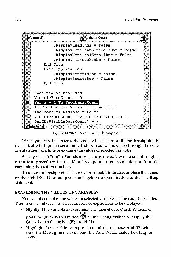
276 Excel for Chemists
Figure 14-20. VBA code with a breakpoint.
When you run the macro, the code will execute until the breakpoint is reached, at which point execution will stop. You can now step through the code one statement at a time or examine the values of selected variables.
Fu Since you can’t “run” a Functi
nction procedure is to add on a
procedure, the only way to step through a breakpoint, then recalculate a formula
containing the custom function.
To remove a breakpoint, click on the breakpoint indicator, or place the cursor on the highlighted line and press the Toggle Breakpoint button, or delete a Stop statement.
EXAMINING THE VALUES OF VARIABLES
You can also display the values of selected variables as the code is executed. There are several ways to select variables or expressions to be displayed:
l Highlight the variable or expression and then choose Quick Watch... or <:I ~:>.*Q.?.$~~..j, ) $$%$~~?~~~,y press the Quick Watch button ~~~ on the Debug toolbar, to &splay the ;\r 3 (.:&pr.:. ( $.> Quick Watch dialog box (Figure 14-21).
l Highlight the variable or expression and then choose Add Watch... from the Debug menu to display the Add Watch dialog box (Figure 14-22).

Chapter 14 Programming with VBA 277
To see the values of the selected variables or expressions, you must be in Step mode. The variables will be listed in the Watches pane (Figure 14-23), which is usually located below the Code window. The current values of the variables will be displayed as you step through the code.
Figure 14-21. The VBA Quick Watch dialog box.
Figure 14-22. The VBA Add Watch dialog box.
Figure 14-23. The VBA Watches pane.

278 Excel for Chemists
To remove a variable or expression from the Watches pane, select it in the Watches pane, choose Edit Watch from the Debug menu, then press DELETE.
Watch expressions are not saved with your code.
USING CONDITIONAL WATCH
A conditional watch expression causes VBA to enter break mode only when a variable changes in value or when an expression evaluates to Tr u e .
To establish conditional watch expressions, choose Add Watch from the Debug menu and press the appropriate Watch Type button (see Figure 14-22). There are three possibilities, which are indicated by different icons in the Watches pane:
bd Watch expression (current value is displayed in the Watches pane when VBA enters break mode)
Conditional break expression (break occurs when expression is True)
& Conditional break expression (break occurs when expression changes)
Excel Tip. You can adjust the widths of the Expression, Value and Context columns in the Watches pane by placing the mouse pointer on the separator bar
to the left of the Value or Context header; the pointer will change to the e pointer shape, and you can drag the separator bar to adjust the column width.
USEFUL REFERENCES Microsoft Excel Visual Basic Reference, 2nd edition, Microsoft Press, 1995. A useful reference - the same information as On-line Help.
Reed Jacobson, Microsoft Excel 2000 Visual Basic for Applications : Fundamentals, Microsoft Press, Redmond, WA, 1999.
John Walkenbach, Excel 2000 Programming for Windows for Dummies, IDG Books Worldwide, San Mateo, CA, 1999. A good book for beginners in VBA programming.
John Walkenbach, Microsoft@ Excel 2000 Power Programming with VBA, IDG Books Worldwide, San Mateo, CA, 1999.

15 WORKING WITH ARRAYS IN VBA
Many scientists make extensive use of arrays in their calculations. Because arrays in VBA can be quite confusing, this chapter provides detailed coverage of this important topic.
VISUAL BASIC ARRAYS If you’re familiar with other programming languages you are probably
familiar with the concept of an array. An array is a collection of related variables denoted by a single name, such as Sample. You can then specify any element in the array by using an index number: Sample(l), Sample(Y), etc.
DIMENSIONING AN ARRAY
The Dim statement is used to declare the size of an array. Unless specified otherwise, VBA arrays begin with an index of 0. The statement
Dim Sample( 10)
establishes array storage for 11 elements, Sample(O) through Sample(l0).
You can specify the lower bound of an array in the Dim statement. For example,
Dim Sample (1 To 10)
allows you to specify any value, even negative values, for the lower or upper bounds of an array. Alternatively, you can use the Option Base 1 statement, which specifies that all arrays begin with a lower index of 1. The Opt ion Base 1 statement is used at the module level: that is, it must appear in a module sheet ahead of any procedures.
Excel Tip. Since worksheet ranges, worksheet functions and worksheet arrays use (or assume) a lower array index of 1, you should always include the Option Base I statement at the beginning of each code module that uses arrays.
Several variables can be dimensioned in a single Dim statement.
279
Excel for Chemists: A Comprehensive Guide. E. Joseph BilloCopyright 2001 by John Wiley & Sons, Inc.
ISBNs: 0-471-39462-9 (Paperback); 0-471-22058-2 (Electronic)

280 Excel for Chemists
It’s considered good programming practice to put the Dim statements at the beginning of the procedure.
USE THE NAME OF THE ARRAY VARIABLE
TO SPECIFY THE WHOLE ARRAY
You can refer to the complete array by using the array variable name in your code. Sometimes the array name can be used with parentheses, other times without parentheses.
MULTIDIMENSIONAL ARRAYS
Arrays can be multidimensional. Excel permits arrays with up to 60 dimensions; one-, two- and three-dimensional arrays are common. To create a 2- D array with dimensions 2 x 500, use the statement
Dim Spectrum (2,500)
Since multidimensional arrays such as the one above can use up significant amounts of memory, it’s important to define the data type of the variable. The complete syntax of the Dim statement is
Dim VariableName(Lower To Upper) As Type
The optional Lower To can be omitted. Type can be Integer, Single, Double, Variant, etc. See the complete list of data types in “VBA Data Types” in chapter 13.) A Variant array can hold values of different data types (e.g., 1.173 and “Billo, E. Joseph”).
mu Several variables can be dimensioned in a single Dim statement, but there
st be a separate As Type for each variable.
RETURNING THE DIMENSIONS OF AN ARRAY
Use the LBound and UBound functions to obtain the dimensions of an array during execution of your procedure. The LBound function returns the lower index
previously, of an array. For example, for the array Sample described LBound(Sample) returns 1 and UBound(Sample) returns 10.
The complete syntax of LBound and UBound is LBound dimension). For the array Spectrum dimensioned thus:
Dim Spectrum (2,500)
,(arrayname,
the statement UBound(Spectrum,l) returns 2 and UBound(Spectrum,2) returns 500 .
DYNAMIC ARRAYS
If you don’t know what array size you will need to handle a particular

Chapter 15 Working with Arrays in VBA 281
problem, you can create a dynamic array. This will allow you to declare a variable as an array but set its size later. Dimension the array using the Dim command, using empty parentheses; use the ReDim command later to specify the array size, e.g.,
Dim MeanX(), MeanY()
‘Get number of cells to use in calculation Ncells = XValues.Count ReDim MeanX(Ncells), MeanY(Ncells)
You can also use the ReDim command to change the nurnber of dimensions of an array.
The ReDim command can appear more than once in a procedure.
PRESERVING VALUES IN DYNAMIC ARRAYS
You can also use the ReDim statement to re-size an existing array during execution of the code. For example, your procedure initially may need an array of 5 x 2000 elements, but later, during execution on a particular data set, a much smaller number of array elements may be needed. You can free up memory by re- sizing the array during execution. However, the ReDim statement re- initializes the array (numbers are set to zero, strings to null, objects to Nothing, for example). You can preserve the values in an existing array by using the Preserve keyword, e.g.,
Dim MeanX(), MeanY()
ReDim Preserve MeanX(Ncells / 2), MeanY(Ncells / 2) But, there’s a limitation. Only the upper bound of the last dimension of a
multidimensional array can be changed. Thus, the following code is valid:
Dim BothMeans(2, 1000)
ReDim Preserve BothMeans(2,Ncells / 2)
but the following code will generate a run-time error:
Dim BothMeans(lOO0, 2)
ReDim Preserve BothMeans(Ncells / 2, 2)
If you use Preserve, you can’t use the ReDim command to change the number of dimensions of an array.

282 Excel for Chemists
WORKING WITH ARRAYS IN SUB PROCEDURES: PASSING VALUES FROM WORKSHEET TO VBA MODULE
There are at least two ways to get values from a worksheet into a VBA array. You can either set up a loop to read the value of each worksheet cell and write the value to the appropriate element of an array, or you can assign the VBA array to a worksheet range. These two methods are described next. There is a definite difference with respect to speed. (See “Speed Differences in Reading or Writing Arrays Created by Two Different Methods” later in this chapter.)
USING A LOOP TO TRANSFER VALUES
FROM A WORKSHEET TO A VBA ARRAY
The Sub procedure shown in Figure 15-1 reads values from worksheet cells and writes them to elements of a VBA array by means of a loop. Either the Cells method or the Range method can be used; in the example that follows, the Range method is used, with the concatenation operator, to access the appropriate cell in the range. In this example the values to be copied are in column A, beginning in row 2. To illustrate an additional point, the values extend down to a row that must be determined by the VBA code.
The code to obtain the row number of the last-used row in the block of cells in column A was obtained by using the Recorder to record the VBA code corresponding to CONTROL+SHIFT+(down arrow).
Sub ArrayDemo () ‘Reads values from column A, beginning in row 2, ‘into a VBA array. I++++++++++++++++++++++++++++++++++++++++ Dim TestArray LastRow = Range(“A2”).End(xlDown).Row NCells = LastRow - 1 ReDim TestArray(NCells) For x = 2 To LastRow TestArray(x - 1) = Range(“A” & x) Next x MsgBox “First array element = ” & TestArray(1) & Chr(13) & _ “Last array element = ” & TestArray(NCells) End Sub
Figure 15-l. Reading values into a VBA array.

Chapter 15 Working with Arrays in VBA 283
A RANGE SPECIFIED IN A SUB PROCEDURE
CAN BE SET EQUAL TO AN ARRAY VARIABLE
If a variable in a VBA Sub procedure is set equal to a range of cells in a worksheet, that variable becomes an array. No Dim statement is necessary. Thus the following expression in Figure 15-2 creates a VBA array called TestArray:
TestArray = Range(“A2:AlO”)
The worksheet array can be a range reference or a name that refers to a reference. Thus, if the name XRange had been assigned to the range ” A2 : A 10 ‘I, then the following expression would also create a VBA array called TestArray:
TestArray = Range(“XRange”)
A one-row or one-column reference becomes a one-dimensional array; a rectangular range becomes a two-dimensional array of dimensions a rray(ro ws, columns).
The lower index of these arrays is always 1. Although arrays created within VBA have a lower array index of zero unless specified otherwise (by means of the Option Base 1 statement, for example), when you transfer a range of cells from a worksheet to VBA, an array is created with lower arrav
J
index of 1.
Sub ArrayDemo ‘Reads values from column A, beginning in row 2, ‘into a VBA array. I++++++++++++++++++++++++++++++++++++++++ TestArray = Range(“A2:AlO”) MsgBox “Fifth array element = ” & TestArray(5, 1) Msg Box “Now changing first array element to zero.” TestArray(5, 1) = 0 Msg Box “Confirming that first array element = ” & TestArray(5, 1) MsgBox “Please examine first array element on worksheet.” End Sub
Figure 15-2. Another way to create a VBA array.
SOME WORKSHEET FUNCTIONS USED WITHIN VBA
CREATE AN ARRAY
If you use a worksheet function within VBA that returns an array, the lower array index will be 1. Such worksheet functions include: LINEST, TRANSPOSE, MINVERSE, MMULT. Other functions that return arrays include the VBA function Caller when used with a menu command or toolbutton.

284 Excel for Chemists
Note that the values in the range of cells have not been transferred to a VBA array; the VBA variable simply “points” to the range on the worksheet.
AN ARRAY OF OBJECT VARIABLES There is an important difference between equating a range of cells in a
worksheet to a simple variable in VBA, thus:
ar = Range(“A2:Bg”)
or equating a range of cells in a worksheet an object variable by using the Set command, thus:
Set ar = Range(“A2:Bg”)
Equating a variable in VBA to a worksheet range automatically creates an array in VBA in which each array element contains the value stored in the cell. Using the Set command to equate an object variable in VBA to a worksheet range automatically creates an array of “cell” objects in VBA. If you change the value of one of the array elements by means of your VBA code, the value in that cell in the worksheet will change, as illustrated by the Sub procedure in Figure 15-3.
For an array of object variables, you must use a different approach to obtain the upper or lower bounds of the array indices, thus:
ar.Rows.Count
or
ar.Columns.Count.
Sub ArrayDemo2aO ‘Reads values from column A, beginning in row 2, ‘into a VBA array of object variables. I++++++++++++++++++++++++++++++++++++++++++ Set TestArray = Range(“A2:AlO”) ,MsgBox “Fifth array element = ” & TestArray(5) MsgBox “Now changing fifth array element to zero.” TestArray(5) = 0 Msg Box “Confirming that fifth array element = ” & TestArray(5) MsgBox “Please examine fifth array element on worksheet.” lend Sub
Figure 15-3. Creating an array of object variables.

Chapter 15 Working with Arrays in VBA 285
WORKINGWITHARRAYSIN SUB PROCEDURES: PASSING VALUESFROM A VBA MODULE TO A WORKSHEET
There are at least two ways to send values from a VBA array to a worksheet. You can either set up a loop and write the value of each array element to a worksheet cell, or you can assign the value of the VBA array to the value of a worksheet range.
USING A LOOP TO TRANSFER VALUES
FROM A VBA ARRAY TO A WORKSHEET
To write the value of each array element to a worksheet cell, you can use either the Cells method or the Range method. In the example shown in Figure 15-4, the Cells method is used.
Sub ArrayDemo ‘Demo to illustrate writing array values to a sheet ‘by means of a loop. I++++++++++++++++++++++++++++++++++++++++++ D i m TestArray( 10) ‘Puts the numbers 11, 12, 13... in a VBA array. For x = 1 To 10: TestArray = 10 + x: Next ‘Then writes the array elements to cells Dl :DlO. For x = 1 To 10 Cells(x, 4).Value = TestArray Next x End Sub
Figure 15-4. Passing values from a VBA array to a worksheet.
This method is straightforward, although sometimes not as convenient the method that follows.
as
EQUATING A WORKSHEET RANGE TO AN ARRAY VARIABLE
In the example shown in Figure 15-5, a 2-D range on a worksheet becomes an array in VBA. Then the array elements are written back to the worksheet with a single line of code.
This is much more convenient than the loop method, where two nested loops would be required to read or write a 2-D range. However, a problem arises when you use this method with a 1-D range, as described next.

286 Excel for Chemists
Sub ArrayDemo ‘Demo to illustrate writing array values to a sheet ‘by writing the array. I++++++++++++++++++++++++++++++++++++++++++ TestArray = ActiveSheet.Range(“Al:B5000”) Range(“D1 :E5000”) = TestArray End Sub
Figure 15-5. Another way to write values from a VBA array to a worksheet.
A&DIMENSIONALARRAYASSIGNEDTOAWORKSHEETRANGE CAN CAUSE PROBLEMS
Arrays can cause some confusion when you write the array back to a worksheet by assigning the value of the array to a worksheet range.
VBA considers a one-dimensional array to have the elements of the array in a row. This can cause problems when you select a range of cells in a column and assign an array to it, as in the Sub procedure shown in Figure 15-6.
Sub ArrayDemo ‘Illustrates that 1-D VBA arrays have elements in a row, ‘not a column. ‘Was supposed to put the numbers 11, 12, 13... in El :ElO. ‘But instead writes element(l) in all cells. I++++++++++++++++++++++++++++++++++++++++++ D i m TestArray( 10) ‘Puts the numbers 11, 12, 13... in a VBA array. For x = 1 To 10: TestArray = 10 + x: Next ‘Then writes the array elements to cells E1:ElO. Range(“E1 :El O”).Value = TestArray End Sub
Figure 15-6. From a VBA array to a worksheet: the row-column problem.
If you run the preceding Sub procedure, you will find that cells El througn El 0 will all contain 11, the first element of the array. However, if you write the array to a row of cells instead of a column, thus:
Range(“E1 :Nl”).Value = TestArray
each cell of the range will receive the correct array value.
There are at least three ways to “work around” this problem caused by “horizontal” and “vertical” arrays. One way is to use a loop to write the elements of the array to individual worksheet cells in a column (Figure 15-7), instead of using the more convenient procedure of assigning the array variable to a range of cells in the worksheet.

Chapter 15 Working with Arrays in VBA
Sub ArrayDemoG() ‘One method to “work around” the row-column problem: ‘write the array elements using a loop. I+++++++++++++++++++++++++++++++++++++++++++++++ Dim TestArray(l0) ‘Puts the numbers 11, 12, 13... in a VBA array. For x = 1 To 10: TestArray = IO + x: Next ‘Then writes the array elements to cells El :ElO. DestRow = 0 : DestCol = 5 For x = 1 To 10 CeIIs(DestRow + x, DestCol) = TestArray Next End Sub
287
Figure 15-7. One method to “work around” the row-column problem.
A second way is to specify both the row and the column dimensions of the array, so as to make it an array in a column, as illustrated in the Sub procedure shown in Fiare 15-8.
Sub ArrayDemo ‘Second method to “work around” the row-column problem: ‘specify the row and column dimensions. I+++++++++++++++++++++++++++++++++++++++++++++++ ‘Puts the numbers 11, 12, 13... in a VBA array. Dim TestArray(l0, 1) For x = 1 To 10: TestArray(x, 1) = 10 + x: Next ‘Then writes the array elements to cells El:ElO. Range(“E1 :El O”).Value = TestArray End Sub
Figure 15-8. A second way to “work around” the rowxolumn problem.
A third way is to use the TRANSPOSE worksheet function (Figure 15-9):
Sub ArrayDemo Another method to “work around” the row-column problem: use Transpose. Note that Transpose creates a l-base array. +++++++++++++++++++++++++++++++++++++++++++++++ Dim TestArray(l0) ‘Puts the numbers 11, 12, 13... in a VBA array. For x = 1 To 10: TestArray = IO + x: Next NewArray = Application.Transpose(TestArray) Range(“E1 :El O”).Value = NewArray End Sub
Figure 15-9. A third way to “work around” the row-column problem.

288 Excel for Chemists
SPEED DIFFERENCES IN READING OR WRITING ARRAYS
CREATED BY TVVO DIFFERENT METHODS
There is a marked difference in the speed of execution of the two methods of reading or writing arrays just described. When you are writing values from a VBA array to a range of worksheet cells, assigning the array name to the range reference, as illustrated by Sub procedure ArrayDemo4, is much faster than using a loop, as in ArrayDemo3. The same is true when you are reading worksheet cells into a VBA array. However, VBA code that involves accessing the individual array elements (such as s umming or comparing all the elements of an array) executes much faster when the cell values have been read into elements of a VBA array that was declared by means of a Dim statement. Thus if your arrays are large, the method you use to “create” the array should be guided by what you intend to do with the array.
WORKING WITH ARRAYS IN FUNCTIONPROCEDURES: FROMWORKSHEET To MODULE
an You can create Function
array as a result. procedures that use arrays as arguments, or return
A RANGE PASSED TO A FUNCTION PROCEDURE
AUTOMATICALLY BECOMES AN ARRAY
If a range argument is passed in a function macro, the range automatically becomes an array in the VBA procedure. No Dim statement is necessary. Thus the expression
Function Deming(XValues, Yvalues)
passes the worksheet ranges XValues and Yvalues to the VBA procedure where they become arrays.
A one-row or one-column reference becomes a one-dimensional array; a rectangular range becomes a two-dimensional array of dimensions array(rows, columns).
The Function procedure in Figure 15-10 is identical to Excel’s INDEX worksheet function: it passes a range and a number as arguments and returns the xth element of the array.
The name of the array in the procedure must be the name of the placeholder argument of the function.

Chapter 15 Working with Arrays in VBA
IFunction ArrayDemog(ArrayRef, x) (‘Shows how to pass an array as an argument. I+++++++++++++++++++++++++++++++++++++++++++++++ ArrayDemo = ArrayRef(x) End Function
Figure 15-10. Passing an array as an argument in a Function procedure.
PASSING AN INDEFINITE NUMBER OF ARGUMENTS
USING THE PARAMARRAY KEYWORD
Occasionally a Function procedure needs to accept an indefinite number or arguments. The SUM worksheet function is an example of such a function; its syntax is =SUM(numberl ,number2,...). To allow a Function procedure to accept an indefinite number of arguments, use the ParamArray keyword in the argument list of the function, as in the following expression
289
Function ConcatenateSpeciaI(ParamArray String1 0)
Only one argument can follow the Pa r a m Array keyword, and it must be the last one in the function’s list of arguments. The argument declared by the Pa ra m Ar r ay keyword is an array of Variant elements. Empty parentheses are required.
Interestingly, even if you use the Option Base 1 statement, the lower bound of the array is zero.
Elements in the array of arguments passed using the Pa r a m Array keyword can themselves be arrays.
RETURNING AN ARRAY OF VALUES AS A RESULT
There are seve ral ways to enable a Function proced values. The most obvious is to assemble the va .lues in
ure to return an array of arrav and return the
array. The procedure shown in Figure 15-11 illustrates a function that returns an array of values: the letters a, b, c and d in a 2 x 2 array. The function requires no arguments. The user must select a 2 x 2 range of cells, enter the function and press, CONTROL+SHIFT+ENTER.
A second approach is to use the Array keyword. The Array function returns a variant that contains an array. In the Sub procedure shown in Figure 15-12, the variable MyArray contains an array of text values, but an array can contain text, number values, the value of a VBA variable, even a Range reference.
To use this function the user must select a horizontal range of cells, enter the function, and press CONTROL+SHIFT+ENTER.

290 Excel for Chemists
Function ArrayDemo 10 ‘Shows one way to return an array of values: ‘Create an actual array by using the Dim statement. I+++++++++++++++++++++++++++++++++++++++++++++++ Dim ReturnValu(2, 2) ReturnValu(1, 1) = “a” ReturnValu(1, 2) = “b” ReturnValu(2, 1) = “c” ReturnValu(2, 2) = “d” ArrayDemo 1 = ReturnValu() End Function
Figure 1541. A Function procedure that returns an array.
Function ArrayDemo 20 ‘Shows another way to return an array of values: the Array keyword ‘Array returns a single variable of Variant type ‘that contains an array. ‘Only 1 -dimensional array, though. I+++++++++++++++++++++++++++++++++++++++++++++++ MyArray = Array(“Jan”, “Feb”, “Mar”, “Apr”, “May”, “Jun”, _ II Jul II “Aug”, “Sep”, “Ott”, “Nov”, “Dee”) ArrayDemo 1 = MyArray End Function
Figure 1542. Using the Array keyword in a Function procedure.
The A r ray keyword can accommodate only a one-dimensional array. To use this approach to return a two-dimensional array, you can create an array of arrays, as illustrated in Figure 15-13. This function returns the letters a, b, c and d in a 2 x 2 array.
Function ArrayDemo 30 ‘Shows another way to return a 2-D array of values. ‘Use the Array function in a nested fashion.
, ArrayDemo 3 = Array(Array(“a”, “b”), Array(“c”, “d”)) End Function
Figure 1543. Using the Array keyword to return a 2-D array.
In each of the preceding examples, you must select an appropriate range of cells to contain the result, enter the function, and press CONTROL+SHIFT+ENTER (Excel for Windows) or CONTROL+SHIFT+RETURN (Excel for the Macintosh).

16 CREATING COMMAND MACROS
A command macro (a Sub procedure) can automate any sequence of actions that can be performed by the use of menu commands or keystrokes. Many simple but useful command macros can be created entirely by using the Recorder, as described in Chapter 13. But command macros can also carry out much more complicated actions. In this chapter we’ll look at some examples of creating more advanced Sub procedures.
CREATING ADVANCED MACROS IN VBA There are literally hundreds of VBA objects, properties and methods, and
this can be confusing for the beginner. Chapter 14 focused on the basic tools needed to create macros to automate chemical worksheet calculations: how to transfer values from a sheet to a VBA module, how to perform calculations within a VBA module, how to perform logical branching and iterative looping, and how to send values back from a VBA module to a worksheet. In this chapter we’ll use these tools to create some useful Sub procedures.
CREATINGA SUB PROCEDURE TOFORMATTEXTASACHEMICALFORMULA
As a first example, we’ll create the ChemicalFormat macro to format text in a selected cell as a chemical formula. The macro will be a simple one. It will examine each character of a text string; if the character is a number, the character will be subscripted. You’ll find this macro useful if you label rows or columns in your worksheets with chemical formulas, such as “CH,CH=CH,” or “moles of H,PO,“; the macro will be a real timesaver.
We need to accomplish four steps in this procedure: (i) obtain the contents of the active cell, (ii) set up a loop so that we can examine each character in turn, (iii) test to see if the character is a number and (iv) subscript the character.
The code required for the first three steps was described in Chapter 14. We’ll (i) use the ActiveCell keyword to obtain the string, (ii) use For... Next to create a loop and the Mid function to access each character within the
291
Excel for Chemists: A Comprehensive Guide. E. Joseph BilloCopyright 2001 by John Wiley & Sons, Inc.
ISBNs: 0-471-39462-9 (Paperback); 0-471-22058-2 (Electronic)

292 Excel for Chemists
loop and (iii) use an If statement to test each character. The only bit of code we’ll need that wasn’t described in Chapter 14 is the code to subscript a character. You could spend some time looking in the VBA On-line Help, but a much easier way to obtain the correct code is to use the Recorder. Simply turn an the Recorder, perform the action of subscripting a character, then go to the Visual Basic Editor and examine the recorded code. You’ll find that the expression to subscript specified characters in a text string in the active cell uses the Characters(start, length) method to specify the characters:
object.Characters(start, /ength).Font.Subscript = True
Simply Copy the code fragment and Paste it into your macro.
The complete macro is shown in Figure 16-l. Right now you’ll have to use the Macro Run dialog box to run the macro, which isn’t very convenient. Of course you could assign a shortcut key to the macro, as described in Chapter 13. In Chapter 19 you’ll learn how to create a custom toolbutton and assign the macro to it.
Sub ChemicalFormat () For x = 1 To Len(ActiveCell) char = Mid(ActiveCell, x, 1) If Asc(char) >= 48 And Asc(char) c= 57 Then ActiveCell. Characters(Start:=x, Length:=l).Font.Subscript = True - Next x End Sub
Figure 16-1. A simple Sub procedure to format text as a chemical formula.
ADDING ENHANCEMENTS TO THE CHEMICALFORMAT MACRO
The simple macro in Figure 16-1 formats the text in a single cell. We’d like our macro to be able to format text in a single cell or in a range of cells. To do this, we simply need to add an outer For..Each...Next loop. We’ll add the lines of code
For Each ccl In Selection
and
Next ccl
at the beginning and the end, respectively, of the original macro, and change three instances of ActiveCell to tel. Note that in the For Each ccl In Selection loop shown in Figure 16-2, the variable ccl is an object variable; thus we can use the code
cel.Characters(Start:=x, Length:=l).Font.Subscript = True

Chapter 16 Creating Command Macros 293
In addition, the macro subscripts every number character in a string. We’d like our macro to be able to handle formulas of hydrates (e.g., CuS04m5H,0) or other text strings containing numbers that should not be subscripted, such as “CaSOJ/2H,O” or “H,PO, (85%)“. The Sub procedure in Figure 16-2 includes code that handles these situations, by using a logical variable FirstFlag. Number characters are subscripted only when FirstFlag = True, and FirstFlag is set to False when any of the special characters are encountered while looping through the string.
Sub ChemicalFormatZ() For Each ccl In Selection FirstFlag = True
For x = 1 To Len(cel) char = Mid(cel, x, 1) If IsNumeric(char) Or char = ‘7 Then
If FirstFlag = True Then GoTo EndLoop If char = ‘7 Then GoTo EndLoop cel.Characters(Start:=x, Length:=l).Font.Subscript = True
Else FirstFlag = False If char = ” ” 0 r char = “*‘I 0 r Asc(char) = 165 0 r char = ‘I,” - Or char = “(” Or char = ‘7” Then FirstFlag = True
End If EndLoop: Next x Next ccl End Sub
Figure 16-2. The ChemicalFormat macro with some additional features added.
Some examples of text formatted by using the ChemicalFormat macro are shown in Figure 16-3.
Figure 16-3. Some examples of formatting with the ChemicalFormat macro.
ADDING MORE ENHANCEMENTS
Finally, we’d like our macro to be able to format text in a worksheet cell or range, in a chart title, or in a textbox. As well, we don’t want the macro to crash

294 Excel for Chemists
Sub ChemicalFormat3() ‘Formats text, e.g., H2S04, as a chemical formula (subscripts numbers). ‘Operates on a cell, a range of cells, text in a chart, or a textbox. ‘Last modified g/22/00 ‘MAKE SURE WE ARE ON A WORKSHEET OR CHART SHEET If TypeName(ActiveSheet) <> “Worksheet” And TypeName(ActiveSheet) <> “Chart” Then Beep:-Exit Sub ‘GO TO CORRECT CODE FOR SELECTION TO BE FORMATTED Select Case TypeName(Selection) Case “Range” ‘FORMAT TEXT IN A CELL OR RANGE
For Each ccl In Selection Call DoFormat(cel.Value, ccl) Next ccl Exit Sub
Case “AxisTitle” ‘FORMAT TEXT IN A CHART Call DoFormat(SeIection.Characters.Text, Selection) Exit Sub
Case “ChartTitle” ‘FORMAT TEXT IN A CHART Call DoFormat(Selection.Characters.Text, Selection) Exit Sub
Case “TextBox” ‘FORMAT TEXT IN A TEXT BOX Call DoFormat(Selection.Characters.Text, Selection) Exit Sub
End Select End Sub
~Sub DoFormat(FormulaString, FormulaObject) FirstFlag = True
For x = 1 To Len(FormulaString) char = Mid(FormulaString, x, 1) If IsNumeric(char) Or char = ‘I.” Then
If FirstFlag = True Then GoTo EndLoop If char = ‘I.” Then GoTo EndLoop
~ FormulaObject.Characters(Start:=x, Length:=l).Font.Subscripl = True ~ Else
~ FirstFlag = False
If char = ” ” 0 r char = “*‘I 0 r Asc (char) = 165 0 r char = “)I’ - Or char =
~ End If “(” Or char = ‘7” Then FirstFlag = True
, EndLoop: Next x End Sub
Figure 16-4. The ChemicalFormat macro with some additional features added.

Chapter 16 Creating Command Macros 295
if we attempt to run it when no sheet is active, for example. The Sub procedure shown in Figure 16-4 uses the VBA keywords TypeName(ActiveSheet) and TypeName(Selection) to determine that the correct kind of sheet is active and that an appropriate selection has been made, before attempting to format the selection.
To develop the code to handle text in a chart or in a text box, a one-line Sub procedure containing either
Msgbox TypeName(ActiveSheet)
Msgbox TypeName(Selection)
was used to display the keywords associated with selected chart elements or a text box. Again, this was faster and more convenient than looking in reference books or using the On-line Help. Once the correct keywords had been found, i t was a relatively simple matter to modify ChemicaIFormat2 to handle text in different environments.
The inner-loop code in Figure 16-2 was used as a general subroutine (now called DoFormat) to examine the text, find the number characters and format them. The main program simply ensures that a worksheet or chart is active, determines the kind of text to be formatted, then calls the subroutine. The subroutine call passes two arguments, a simple variable containing the text to be examined (FormulaString) and an object variable containing the text to be subscripted (FormulaObject).
Since several different kinds of text were to be formatted, a Select Case construction was used. As it turned out, the same syntax is used to subscript text in a chart or in a text box. Nevertheless, the original Select Case structure was left in place.
CREATINGA SUB PROCEDURE TO APPLY DATALABELSINACHART
As described in Chapter 5, the Data Labels tab in the Format Data Series dialog box allows you to add data labels to a chart (to each data point in an XY chart, or to each column in a column chart, for example). But only the x values or the y values can be used as labels. You’d probably like to use some other text as data labels. You can do this manually, by adding the data labels, then manually editing each one to enter the text you want. A macro will make the task much easier.
In the following section we will develop a Sub procedure to assign text values in a range of cells as the data labels for a chart. Here’s how we’ll proceed: we’ll use the Recorder to obtain the code for adding data labels,

296 Excel for Chemists
selecting a data label and entering text. We’ll use this code as a framework cn which to construct our macro.
The code shown in Figure 16-5 was obtained when the Recorder was used to record the following actions: selecting a chart, selecting a data series, choosing Selected Data Series from the Format menu and applying data labels, selecting a data label, and typing the text “abc” in place of the original label. In this Sub procedure we have almost all the code we need to create the initial version of our macro.
Sub Macro1 () Macro recorded g/25/00 by Dr. Billo
ActiveSheet.ChartObjects(“Chart l”).Activate ActiveChart.SeriesCollection(l).Select ActiveChart.SeriesCollection(l).ApplyDataLabels Type:=xlDataLabelsShowValue, AutoText:=True, LegendKek=False ActiveChart.SeriesCollection(l).DataLabels.Select ActiveChart.SeriesCollection(l).Points(4).DataLabel.Select Selection.Characters.Text = “abc” Selection.AutoScaleFont = False With Selection.Characters(Start:=l, Length:=3).Font
.Name = “Geneva”
.FontStyle = “Regular”
.Size = 10
.Strikethrough = False
.Superscript = False
.Subscript = False
.OutlineFont = False
.Shadow = False Underline = xlUnderlineStyleNone Colorlndex = xlAutomatic
End With ActiveChart.ChartArea.Select
End Sub
Figure 16-5. Macro1 recorded.
In the first version of our macro, the chart must be the active document, and the user must have selected the data series to which the data labels are to be attached before running the macro. In a later version we’ll allow the user to select the data series while the macro is running.
The four lines of code from M acre 1 that we’ll use (after modifying them) are as follows:
ActiveChart.SeriesCollection(l).ApplyDataLabels Type:=xlDataLabelsShowValue, AutoText:=True, LegendKeF=False
ActiveChart.SeriesCollection(l).DataLabels.Select

Chapter 16 Creating Command Macros 297
ActiveChart.SeriesCollection(l).Points(4).DataLabel.Select
Selection.Characters.Text = “abc”
To complete our macro, we’ll need to add some code (i) so that the user can specify a range of cells that contain the labels, (ii) to set up a loop so that we can loop through all the data points and (iii) to change SeriesCollection( 1) to the general case.
To specify the range of cells to use as data labels, we’ll use the lnpu t Box method. We’ll define the range as an object variable, so that we can use a For...Each...Next loop. For a code example, see “You Can Define Your Own Objects” in Chapter 14. To convert SeriesCollection(1) into the general case, remember that a specific item in a collection can be referred to by its index number or by its name. We’ll use the code
SeriesName = Selection.Name
and
ActiveChart.SeriesCollection(SeriesName)
to specify the selected data series.
After the macro was completed, some testing revealed that in most cases, the code containing the Select keyword could be eliminated. The completed macro is shown in Figure 16-6.
Sub Labeler1 () ’ Get the name of the chart data series. SeriesName = Selection.Name
’ Input the range of cells to be used as labels. Set LabelRange = Application.lnputBox(“Select the range of cells containing the labels”, “DATA LABELER STEP 1 OF l”, , , , , , 8)
’ Apply the standard data labels. ActiveChart.SeriesCollection(SeriesName).ApplyDataLabels Type:=xlDataLabelsShowValue, AutoText:=True, LegendKey:=False -
’ Set up a loop to replace data labels with new ones. X =l For Each ccl In LabelRange
ActiveChart.SeriesCollection(SeriesName).Points(x). _ Datatabel. Characters.Text = cel.Value
X =x+1 Next ccl End Sub
Figure 16-6. The completed DataLabeler macro.

298 Excel for Chemists
A more sophisticated version of the macro can be found on the CD-ROM that acompanies this book.

17 CREATING CUSTOM FUNCTIONS
Chapter 13 provided an introduction to Sub procedures and Fu net i o n procedures. By now it should be clear that a Sub procedure (a command macro) is a computer program that you “run”; it can perform actions such as formatting, opening or closing documents, etc. A Function procedure (a user-defined function) is a computer program that calculates a value and returns it to the cell in which it is typed. A Function procedure cannot change the worksheet environment ( e.g., it can’t make a cell Bold).
The following sections provide some examples of more advanced custom functions.
A CUSTOMSTATISTICALFUNCTION One of the underlying assumptions of the least squares method is that there
is no error in the measurement of the independent variable (the y values). This assumption is often not valid, and one of the most obvious cases of this is found in method-comparison analysis. A typical example of method-comparison analysis involves the comparison of two different instruments, a current production instrument and an improved model. Measurements made on a series of samples with the two instruments, and plotted by using current instrument readings as the x values and new instrument readings as the y values, should ideally result in a straight line of unit slope and zero intercept. The actual slope and intercept of the line can provide estimates of the proportional and constant error between the two methods.
It is obvious that there is error in both the x and the y values. Calculation of the least-squares slope and intercept by “standard” methods is clearly not valid. In the custom function that follows, the method of Deming is used to calculate the regression parameters for the straight line y = mx + b. The Deming regression calculation assumes Gaussian distribution of errors in both x and y values and uses duplicate measurements of x values (and of y values) to estimate the standard errors. A portion of a data table is shown in Figure 17-1.
299
Excel for Chemists: A Comprehensive Guide. E. Joseph BilloCopyright 2001 by John Wiley & Sons, Inc.
ISBNs: 0-471-39462-9 (Paperback); 0-471-22058-2 (Electronic)

300 Excel for Chemists
II 44.35 23.45 29.45 46.70 48.05 27 65 27.30 27.05 26.90
Y
24 95 26.55 21.70 22.20 44.60 44 .## 29 .m 30 .uo 47.45 47.20 26.45 27.25
Figure 17-I. Portion of data table to calculate Deming regression parameters.
The equations*for the Deming slope and intercept are
m=U+ u +(1/h) r
and b=ij -mf-
where u - s; -(l/A)s; -
2rsxsy
h s 2
- t?X -
S2 eY
X and f are the means and $1 S;are the variances of the xmean and ymean
values, respectively, Y is the Pearson correlation coefficient and Szx and Szy are
the error variances of the x values and y values, respectively, calculated from the equation
se = Z(difference between duplicates)2
2N
* See, for example, I? J. Cornbleet and N. Gochman, Clin. Chem. 1979,25,432.

Chapter 17 Creating Custom Functions 301
Deming Regression Calculates Deming regression parameters for Y = mX + b Equations from Cornbleet & Gochman, Clin. Chem. 1979, 25, 432. Copyright 1997 by E. J. Bill0 Begun WI O/97. Last modified 1 O/3/00
Qnction Deming(XValues, Yvalues) Xm MeanX(), MeanY() Get number of cells to use in calculation loop \Icells = XValues.Count 3eDim MeanX(Ncells / 2), MeanY(Ncells / 2)
Step thru pairs of cells, calculating sums for statistics talcs :or x = 2 To Ncells Step 2
MeanX(x I 2) = (XValues(x - 1) + XValues(x)) I 2 MeanY(x / 2) = (Yvalues(x - 1) + Yvalues(x)) / 2 SumX = SumX + MeanX(x / 2): SumY = SumY + MeanY(x / 2) SumX2 = SumX2 + (MeanX(x / 2)) * 2 SumY2 = SumY2 + (MeanY(x / 2)) A 2 SumXY = SumXY + MeanX(x / 2) * MeanY(x I 2) SumDeltaX2 = SumDeltaX2 + (XValues(x - 1) - XValues(x)) * 2 SumDeltaY2 = SumDeltaY2 + (Yvalues(x - 1) - Yvalues(x)) * 2
Vext
Calculate some intermediate statistical quantities <Bar = SumX / N: YBar = SumY / N 5x2 = (N * SumX2 - SumX A 2) / (N * (N - 1)) Sy2 = (N * SumY2 - SumY A 2) / (N * (N - 1)) Sdx2 = SumDeltaX2 / (2 * N) Sdy2 = SumDeltaY2 / (2 * N) *Pearson = (N * SumXY - SumX * SumY) / Sqr((N * SumX2 - SumX * 2) * (N * SumY21 SumY * 2))
Calculate quantities that are specific to the Deming calculation ambda = Sdx2 I Sdy2 J = (Sy2 - Sx2 / lambda) / (2 * rPearson * Sqr(Sx2) * Sqr(Sy2)) Slope = U + Sqr(U A 2 + 1 / lambda) ntercept = YBar - Slope * XBar
Ieming = Array(Slope, Intercept) End Function
Figure 17-2. A Function procedure to calculate Deming regression parameters.

302 Excel for Chemists
The macro listing is shown in Figure 17-2. The two arguments used by the macro are a range of cells containing pairs of x measurements on a given sample and a corresponding range of pairs of y measurements.
Within the procedure, the major part of the code is virtually identical to the code that would be used to obtain the usual least-squares regression parameters for y = mx + b, namely, obtaining the sum of x values, the sum of squares of x values, etc. The difference is that pairs of values are used; the mean value of each pair of x values or of y values is used as the independent variable or dependent variable, respectively, and the estimate of the standard errors for the two sets of data is obtained from the differences between pairs.
Near the end of the code some calculations that are specific to the Deming equations are performed. The function returns an array of two values, the slope and intercept of the Deming regression. Since an array is returned, the user must press CONTROL+SHIFT+ENTER (Windows) or CONTROL+SHIFT+RETURN (Macintosh).
This function could be located in the Statistical category, rather than in the User Defined category. See “Assigning a Custom Function to a Function Category” later in this chapter.
A CUSTOMFUNCTIONTHATTAKES ANOPTIONALARGUMENT
A custom function can have optional arguments. Use the Optional keyword in the list of arguments to declare an optional argument. The optional argument or arguments must be last in the list.
You will need to determine the presence or absence of optional arguments in a procedure by using the IsMissing keyword. As well, you may need to provide a default value if an argument is omitted.
In the example shown in Figure 17-3, the custom function MolWt calculates the formula weight of a compound from formula (a text string in a cell). The formula weight is calculated in the subroutine Parse (not shown), which returns FW, the formula weight, and NumDecimals, the number of decimal places allowed in the result, based on the atomic weights used. The user can specify, by the optional argument decimals, the number of decimal places to be displayed in the returned value. If the optional argument decimals is not supplied, the function returns the value of FW, but if decimals is supplied, the worksheet function FIXED is used to set the number of decimal places in the result.
The MolWt function can be found on the CD-ROM that acompanies this book.

Chapter 17 Creating Custom Functions 303
Function MolWt(formula As String, Optional decimals) ’ If decimals is omitted, returns value as a number. ’ If decimals is specified, returns value as text, ’ formatted with specified number of decimals. ’ Maximum number of decimal places allowed is determined in subroutine ’ by decimal places of atomic weights.
Call Parse(formula, FW, NumDecimals) If IsMissing(decimals) Then MolWt = FW: Exit Function If NumDecimals < decimals Then MolWt = Application.Fixed(FW, NumDecimals): Exit Function MolWt = Application.Fixed(FW, decimals) End Function
-
Figure 17-3. A Function procedure with an optional argument.
A CUSTOM FUNCTION THAT TAKES AN INDEFINITE NUMBER OF ARGUMENTS
Many of Excel’s worksheet functions can accept an indefinite number arguments. The SUM function is an example of such a function; its syntax 1s
=SUM(numberl ,number2,...). To create a custom function with an indefinite number of arguments, use the Pa ram Array keyword. An argument declared with ParamArray is an array of Variants, and each element of the array can itself be an array.
The next example shows a custom function that accepts a number of worksheet ranges as arguments and combines them into a single array. This custom function is designed to be used with Excel’s LINEST function (see Chapter 11). LINEST requires that the known x’s argument be a contiguous range of cells; you can’t use a non-adjacent selection as the argument, even if the ranges are enclosed in parentheses. But when you perform multiple linear regression using several columns of x values, oftentimes those columns of x values are not contiguous, as illustrated in Figure 17-4. The expression =LINEST(E4:E13,(A4:A13,C4:C13),1 ,I) returns the #REF! error message. You could rearrange the worksheet to have all the columns of x values adjacent, but with the custom function shown in Figure 17-5 you can combine the separated ranges into a single array and use it as the known x’s argument of LINEST. -
Since LINEST requires that there be the same number of values for each independent variable, we first check to make sure that each range in the array of arguments has the same number of rows. An interesting point: although we specified 0 lower array
ption index
UBound(rng) iS
Base 1, the ParamArray keyword produces an array whose is zero. Thus we must loop from 0 to UBound(rng). Note that
the number of elements in the array, while

304 Excel for Chemists
rng(z).Columns.Count returns the number of columns in an individual element in the array.
Figure 17-a. LINEST fails when used with a non-adjacent selection of known-x’s
If an array element is not the correct size, we need to return an error value. Use the CVE r r keyword to return a worksheet error value that Excel can handle appropriately. The error values are listed in Appendix D.
After checking all the elements in the array, we assemble them into the final array of dimensions XSize rows by YMax columns, and return the array to the worksheet.
Now the LI N EST expression
=LINEST(E4:E13,MakeArray(A4:A13,C4:C13),1 ,I)
returns the correct result. You can use names for cell ranges in the MakeArray function, e.g.,
=LINEST(YValues,MakeArray(Xvaluesl ,Xvalues2),1 ,l.

Chapter 17 Creating Custom Functions 305
Option Base 1
Function MakeArray(ParamArray rng()) ’ Combines individual I-D or 2-D arrays into a final 2-D array. ’ In this version all individual arrays must be vertical. ’ All individual arrays must have same number of rows.
Dim Result0 As Variant Dim XSize As Integer, YSize As Integer, YMax As Integer
’ Z index is used to select within array of arrays. ’ x and y are column & row indices of individual arrays.
’ First, calculate size of final array. ’ And check to make sure all arrays contain same number of rows. ’ Despite use of Option Base 1, LBound = 0 XSize = rng(O).Rows.Count ‘returns “Base 1” value YMax = 0 For z = 0 To UBound(rng) YSize = rng(z).CoIumns.Count ‘returns “Base 1” value If XSize <> rng(z).Rows.Count Then MakeArray = CVErr(xlErrRef): _ Exit Function
YMax = YMax + YSize Next z ReDim Result(XSize, YMax)
’ Now combine each individual array into final array. YStart = 0 For z = 0 To UBound(rng) YSize = rng(z).CoIumns.Count For y = 1 To YSize For x = 1 To XSize Result(x, YStart + y) = rng(z)(x, y) Next x, y YStart = YStart + YSize Next z MakeArray = Result End Function
Figure 17-5. A Function procedure to combine arrays.

306 Excel for Chemists
PROVIDINGADESCRIPTIONFORA CUSTOMFUNCTION IN THE PASTE FUNCTION DIALOG Box
When you use Paste Function to enter a function, the function’s description appears at the bottom of the dialog box. For a custom function, the default description is “Choose the Help button for Help on this function and its arguments”, but you can provide a custom description for your custom function. There are two ways to do this: you can use the Macro dialog box (normally used only for Sub procedures), or you can write and run a simple one-line VBA Sub procedure. Either way, the description becomes part of Excel and does not need to be entered each time you start Excel.
To use the Macro dialog box to enter a description, carry out the steps in the following box.
To Provide a Description for a Custom Function
1. Choose Macro from the Tools menu and Macros,,. from the submenu.
2. Type the name of the custom function in the Macro Name box.
3. Press the Options... button to display the Macro Options dialog box.
4. Type the description in the Description box, then press OK.
To enter a description by means of VBA code, type and run a Sub procedure similar to the one shown in Figure 17-6.
Sub CustomFunctionDescription() Application.MacroOptions macro:=“FtoC”, Description:= - “Converts Fahrenheit temperature to Celsius” End Sub
Figure 17-6. A Sub procedure to add a function description.
For Excel’s built-in functions, the Formula Palette (Step 2 of Paste Function) provides help information about each argument as you begin to enter it. There’s no way to provide similar information about arguments in the Formula Palette for custom functions. But since the same description text appears in the Step 1 and the Step 2 dialog boxes, you can provide information about the arguments in the description. Unfortunately the limit for Description is 255 characters. You can provide line breaks in the text by using Chr(l0) or Chr(l3), but the Formula Palette can only display two lines of text.

Chapter 17 Creating Custom Functions 307
ASSIGNINGACUSTOMFUNCTION TOAFUNCTIONCATEGORY
Initially, your custom function will be located in the User Defined category in the Paste Function dialog box. You can specify the category in which function will be located, by typing and running a Sub procedure similar to one shown in Figure 17-7. The category values are listed in Appendix D.
the the
Sub CustomFunctionDescription() ApplicationJVfacroOptions macro:=“FtoC”, Category:=3 End Sub
Figure 17-7. A Sub procedure to change function category.
CREATING ADD-IN FUNCTION MACROS Saving a custom function as an Add-In is by far the most convenient way to
use it. Here are some of the advantages:
l An Add-In custom function is listed in the Paste Function list box without the workbook name preceding the name of the function, making it virtually indistinguishable from Excel’s built-in functions.
l If the Add-In workbook is placed in the Excel Startup folder, the Add-In will be available every time you start Excel.
l An Add-In workbook can be hidden so it can’t be viewed by the user.
HOW TO CREATE AN ADD-IN MACRO
To save a workbook as an Add-In, choose Save As... from the File menu. Choose Microsoft Excel Add-In from the Save File As Type drop-down list box, then press OK. In Excel for Windows, Add-In macros are automatically given the filename extension .xla.
Your custom functions will now be indistinguishable from Excel’s built-in functions. By giving them names using lower-case letters, you can distinguish them from Excel’s built-in functions.
Command macros can also be saved as Add-Ins.
HOW TO PROTECT AN ADD-IN WORKBOOK
To protect an Add-In workbook, activate the Visual Basic Editor. Choose Properties... from the Tools menu and choose the Protection tab. Check the Lock Project For Viewing box, enter a password, and Save the workbook.
308
ADVANTAGESANDDISADVANTAGES 0~ USING FUNCTION MACROS
Excel for Chemists
Some function macros perform calculations that could be performed by using a worksheet formula or formulas, while in other cases implementing the function on the worksheet is impossible (when looping or branching is required, for example).
The main advantage of using a custom function instead of worksheet formulas is minimization of errors occurring when formulas are entered. The main disadvantage is that custom functions are slower than worksheet formulas. For example, in a sheet that uses worksheet formulas to calculate the four alpha values for phosphoric acid in 0.1 pH increments from pH 0 to 14 (calculation of 564 cells) using worksheet formulas (see Chapter 20), there was no detectable delay when the sheet was recalculated. On the same PC, when the ALPHA function was used, it took three seconds to recalculate the sheet.

18 CREATING CUSTOM MENUS
AND MENU BARS
In this chapter you’ll learn how to add a new command to a menu, how to add a new menu to a menu bar and how to create a whole new menu bar with separate menus and commands. In this way you can add new capabilities to Excel or even create a complete custom application.
In earlier versions of Microsoft Excel, menu bars contained only menus, and toolbars only toolbuttons. Beginning with Excel 97, toolbuttons and menu items are both members of the class of CommandBarButton objects. Command bars can contain buttons or menus or both. In general, however, mixing buttons and menu commands on the same toolbar doesn’t seem to be a good idea, so this chapter deals exclusively with menus and Chapter 19 with toolbars.
MODIFYING MENUS OR MENU BARS You can modify existing menus or menu bars by using the Customize
command in the Tools menu. Each version of Excel has used a different method to customize menus: Excel 5/95 used the Menu Editor to modify menus, Excel 97 displayed a customizable copy of the menu bar in which to make changes, but in Excel 2000 menus are customized in exactly the same way as toolbars - by dragging the menu command to the desired place on the menu bar.
ADDING OR REMOVING A MENU COMMAND
You can add any of Excel’s built-in menu commands to a menu, or remove menu commands that you don’t use. The procedures in the following boxes cover these possibilities.
Some commands in the list of commands in the Commands tab have an icon beside them, others don’t. Commands with an icon are toolbuttons, and those without an icon are menu commands.
309
Excel for Chemists: A Comprehensive Guide. E. Joseph BilloCopyright 2001 by John Wiley & Sons, Inc.
ISBNs: 0-471-39462-9 (Paperback); 0-471-22058-2 (Electronic)

310 Excel for Chemists
To Add a Built-in Menu Command to a Menu
1. The toolbar that contains the menu to be customized must be visible. 2. Choose Customize. l . from the Tools menu, or choose Toolbars.., from
the View menu and choose Customize.. ., or right-click on any toolbar and choose Customize... from the shortcut menu.
3. (This step necessary only in Excel 97/98.) Choose the Toolbars tab, then check the box for, or double-click on, the Worksheet Menu Bar or Chart Menu Bar to display a customizable copy of the menu bar.
4. Choose the Commands tab.
5. In the Categories box, choose the desired category, then choose the new command from the list in the Commands box and drag it to the desired location in the copy of the menu. The mouse pointer will display a large “X” beside the mouse pointer image if the mouse pointer is over a location at which the command cannot be installed, If the command can be installed, there will be a small ‘T’.
CREATING A NEW MENU BAR
In previous chapters you learned how to create usefulsub procedures. You may find that you use a particular macro so often that it would be more convenient to have it on one of Excel’s drop-down menus, rather than having to “run” it by means of the Run command from the Macro menu. Running a command macro by means of an Excel menu command makes the custom command accessible to Excel users who are not familiar with the use of macros.
If you have written a number of related macros, you may even decide to create a custom menu bar with several custom menus, each containing custom commands. While both “Custom Menu Command” and “New Menu” can be

Chapter 18 Creating Custom Menus and Menu bars 311
found in Customize, there’s no “New Menu Bar”. That’s because menu bars are really toolbars. To create a new menu bar, you simply create a new toolbar and place menus on it instead of toolbuttons.
You can install either custom menus or any of Excel’s built-in menus on your custom menu bar. To install custom menus, follow the procedure in the following box; to install any of Excel’s built-in menus, follow the same procedure but choose “Built-in Menus” from the Categories box. You can apply the same methods used for custom menus to add commands to, remove commands from, or rename the built-in menus. Menus installed on a custom menu bar are displayed with a drop-down arrow next to the menu name. Figure 18-1 shows such a custom menu bar.
Figure 18.1 A custom menu bar with three menus: Excel’s built-in File and Edit menus and a custom menu.
ADDING A CUSTOM MENU TO A MENU BAR
To add a custom menu to a menu bar, use the procedure in the following box
To Add a Custom Menu to a Menu Bar
1. The toolbar that contains the menu to be customized must be visible,
2. Choose Customize.. . from the Tools menu, or choose Toolbars... from the View menu, or right-click on any toolbar and choose Customize.. . from the shortcut menu.
3. (This step necessary only in Excel 97/98.) Choose the Toolbars tab, then check the box for, or double-click on, the Worksheet Menu Bar or Chart Menu Bar to display a customizable copy of the menu bar.
4. Choose the Commands tab. 5. Scroll through the Categories box and choose “New Menu”.
6. Select New Menu and drag it to the desired location on the toolbar. 7. Right-click on the custom menu item to display the shortcut menu.
Type the name of the new menu in the Name input box (the default text is “New menu”).

312 Excel for Chemists
Excel Tip: If you add a built-in menu to a toolbar and make changes to the menu, the changes will also appear in the built-in menu on the menu bar. Thus if you want a modified File menu on a custom menu bar, you should add a custom menu, rename it File, and then add the desired menu commands.
ADDING A CUSTOM MENU COMMAND TO A MENU
To add a custom menu command to a menu, use the procedure in the following box.
When you exit from Excel, any changes you made to the menu bars or toolbars are saved, and this menu bar/toolbar configuration will be displayed the next time vou start Excel.

Chapter 18 Creating Custom Menus and Menu bars 313
MODIFYING MENUS 0~ MENU BARS BY USING VBA You can also modify existing menus or menu bars by using Visual Basic.
If you create a macro to be used by other people, you can make it easy for them to use the macro by installing a custom menu command. As well, you can install the new menu command by means of an automatic procedure, so that all the users have to do is open the macro document. There are two ways you create an automatic procedure: by creating an Auto-Open macro in a module sheet, or by creating a Workbook Open event procedure. These are described in the - sections that follow.
In contrast to changes to menus made by using the Customize... command, menus and menu commands installed by using VBA are not saved when you quit Microsoft Excel.
ADDING A MENU COMMAND BY MEANS OF AN AUTO OPEN MACRO -
In Excel 5/95, any macro with the name Auto Open will be run - automatically whenever the workbook containing that macro is opened. You can still employ Auto Open procedures in Excel 97 or Excel 2000. -
To install a new menu command whenever Excel is started, create an Auto Open procedure in the Personal Macro Workbook. To install a new menu - command when a particular workbook is opened, create an Auto-Open procedure in that workbook. Use the MenuBars and Menus VBA keywords to specify where the new Menultem is to be added, with the Add keyword. The syntax of the Add method is:
MenuItems.Add(caption, onAction, shortcutKey, before)
The text of the menu item that will appear in the menu is Caption. The name of the macro that runs when the new menu item is selected is OnAction. ShortcutKey is available only for Macintosh. If Before, which specifies the position in the menu, is omitted, the command is added at the end of the menu.
Figure 18-2 illustrates an Auto Open procedure that installs a new menu - command in the Tools menu and assigns the Sub procedure named CommandHandler to it. To install your own custom menu command in a menu, replace Tools, New Menu Item and CommandHandler with the name of the menu, the text of your menu command and the name of your macro.
Menu commands installed by this method remain in the menu until you exit from Excel.
Sub AUTO-OPEN0 MenuBars(“Worksheet”).Menus(“Toois”).MenuItems.Add Caption:=“New Menu Item”, OnAction:=“CommandHandler”, Before:=1 End Sub
Figure 18.2 An Auto Open Sub procedure to install a custom menu command. -

314 Excel for Chemists
ADDING A MENU COMMAND
BY MEANS OF AN EVENT-HANDLER PROCEDURE
Event-handler procedures were introduced in Excel 97; they can be used in Excel 97 or Excel 2000. Event-handler procedures provide more versatility than the automatic procedures provided with Excel 5/95.
Event-handler procedures are not written in the usual VBA modules, but in the code modules associated with a worksheet or workbook. For example, to install a new menu command when a particular workbook is opened, put the event-handler procedure in the code window for ThisWorkbook (use the Project Explorer to locate the node for ThisWorkbook, then click on it to display the Code window).
Use the CommandBars VBA keyword to specify where the new Control is to be added, with the Add keyword. The syntax of the Add method is:
Controls.Add(Type, Id, Parameter, Before, Temporary)
Type is msoControlButton. Id and Parameter can be omitted; see VBA On-line Help for an explanation of the use of these arguments. If Before, which specifies the position in the menu, is omitted, the command is added at the end of the menu. Set Temporary to True to make the custom menu command temporary; temporary menu commands remain in the menu until you exit from Excel.
Private Sub Workbook-Open0 This procedure installs a new menu command ‘at the top (the default position) of the Tools menu.
Set NMC = Application.CommandBars(“Tools”).Controls.Add - (Type:=msoControlButton, temporary:=True)
NMC.Caption = “New Menu Command...” NMC.OnAction = “MyProcedure”
End Sub
Figure 18.3. An event-handler procedure to install a custom menu command.
Figure 18-3 illustrates a Workbook - Open procedure that installs a new menu command in the Tools menu and assigns the Sub procedure named MyProcedure to it. In the preceding code, replace New Menu Command... and MyProcedure with the text of your menu command and macro name. In this example, MyProcedure, which simply beeps ten times, is a Sub procedure located in a module sheet (Figure 18-4).
Sub MyProcedure For x = 1 To IO: Beep: Next
IEnd Sub I Figure 18.4. The Sub procedure that runs when the custom menu command is chosen
from the Tools menu.

Chapter 18 Creating Custom Menus and Menu bars 315
Private Sub Workbook-Open0 This procedure installs a new menu command ‘immediately below the Goal Seek command in the Tools menu ‘with a separator bar below it.
posn = Application.CommandBars(“Tools”).Controls _ (“Goal Seek...“).lndex
Set NMC = Application.CommandBars(“Tools”).Controls.Add _ (Type:=msoControlButton, before:=posn + 1, temporary:=True)
NMC.Caption = “New Menu Command...” NMC.OnAction = “MyProcedure”
Set NMC = Application.CommandBars(“Tools”).Controls.Add (Type:=msoControlButton, before:=posn + 2, temporary:=True) -
NMC.Caption = “J’
End Sub
Figure 18.5. An event-handler procedure to install a custom menu command.
You may want to install a new menu command immediately above or below a menu command that is already present in the menu. Since menus can be customized, you shouldn’t use a numerical value for the position; instead, determine the position of the command programmatically. Use the Index property as shown in Figure 18-5.
Use Caption = “2 (the hyphen) to insert a separator bar, with Or-Action:=“” or omitted.
From the preceding examples it should be clear that you can create automatic procedures that install a menu command when a particular workbook is opened and remove the menu command when that workbook is closed (using the Workbook-BeforeClose event procedure). Or you can install a command when a particular worksheet is activated and remove it when that worksheet is deactivated.

19 CREATING CUSTOM TOOLBUTTONS
AND TOOLBARS
In this chapter you’ll learn how to customize Excel’s built-in toolbars and how to create new toolbuttons to simplify some of the operations that you perform often.
CUSTOMIZING TOOLBARS Some of the toolbuttons on Excel’s toolbars are not very useful for scientists.
You can remove the toolbuttons you don’t use, giving a less cluttered workspace and providing room for other, more useful toolbuttons.
MOVING AND CHANGING THE SHAPE OF TOOLBARS
Excel’s toolbars are usually located along the edges of the screen, most commonly along the top edge. Excel initially displays the Standard and Formatting toolbars, which provide tools for common Excel actions. There are a number of other toolbars provided with Excel, including the Chart, Drawing and Forms toolbars. You can also create custom toolbars, containing the tools you use most.
A toolbar can be moved from its position at the top of the screen and placed anywhere on the screen. Simply drag the move handle (located at the left side of a docked toolbar) to another location. A toolbar that is moved from a position along the edge of the screen is called a floating toolbar. It appears in its own window, with a title bar and a Close box (a title bar, Close box and a Size box in the Macintosh version of Excel). If you change the height or width of a floating toolbar, the tools are automatically rearranged to fit the new shape. If a floating toolbar (Figure 19-1) is dragged near the edge of the screen, Excel places it in a toolbar dock There are four toolbar docks, one along each of the edges of the Excel application window.
If a toolbar does not fill the whole window (from left to right or vertically, depending on its orientation) the toolbar dock is visible as the extra blank space at either side of the toolbar, separated from the toolbar by the toolbar border.
317
Excel for Chemists: A Comprehensive Guide. E. Joseph BilloCopyright 2001 by John Wiley & Sons, Inc.
ISBNs: 0-471-39462-9 (Paperback); 0-471-22058-2 (Electronic)

318 Excel for Chemists
Figure 19-1. The Excel 2000 Standard toolbar.
Excel Tip. A toolbar that contains a drop-down list box, such as the cannot be placed in a vertical position in the leff or right toolbar docks.
Style box,
ACTIVATING OTHER TOOLBARS
You can display a toolbar by choosing Toolbars from the View menu, then checking the box for the desired toolbar in the submenu. You can also display a toolbar by choosing Customize... from the Tools menu, choosing the Toolbars tab (Figure 19-2) and checking the box for the desired toolbar.
Remove a toolbar by choosing Toolbars from the View menu and unchecking the box for the toolbar, or by dragging the toolbar from the toolbar dock and then pressing the Close box. You can have several toolbars in the Excel window at once.
Excel Tip. Right-click on any toolbar (Windows) or hold down the CONTROL key and click on any toolbar (Macintosh) to display the Toolbar shortcut menu.
Figure 19-2. Displaying a built-in toolbar with the Toolbars dialog box.

Chapter 19 Creating Custom Tools and Toolbars 319
ADDING OR REMOVING TOOLBUTTONS FROM TOOLBARS
Removing seldom-used toolbuttons from a toolbar provides a less cluttered working environment and makes room for other, more useful tools. To delete a toolbutton from a toolbar or to add a built-in toolbutton to a toolbar, follow the procedures in the following boxes.
To Delete a Toolbutton from a Toolbar
1. Choose Toolbars from the View menu and choose Customize..., or choose Customize... from the Tools menu, or right-click on a toolbar and choose Customize... from the shortcut menu.
2, Drag the toolbutton off the toolbar (when you click on it, the toolbutton outline is highlighted) and release the mouse button. The toolbutton will disappear.
4 4
To Add a Built-in Toolbutton to a Toolbar To Add a Built-in Toolbutton to a Toolbar
1. Choose Toolbars from the View menu and choose Customize..., 1. Choose Toolbars from the View menu and choose Customize..., or choose Customize... from the Tools menu, or right-click on a or choose Customize... from the Tools menu, or right-click on a toolbar and choose Customize... from the shortcut menu. toolbar and choose Customize... from the shortcut menu.
2. Choose the Commands tab. 2. Choose the Commands tab.
3. Select the desired toolbutton from the various categories (Figure 3. Select the desired toolbutton from the various categories (Figure 19-3). Drag the toolbutton to the desired place on the toolbar. 19-3). Drag the toolbutton to the desired place on the toolbar. Spaces between toolbuttons may be added or removed by using Spaces between toolbuttons may be added or removed by using the procedure in the following box. the procedure in the following box.
I ” I ”
The built-in Microsoft Excel toolbars can be restored to their “factory- installed” condition by using the Reset button in the Toolbars tab of the Toolbars dialog box (Figure 19-2). Individual toolbuttons can be restored by following the procedure described earlier. Custom toolbars cannot be reset.
Toolbuttons can be organized into logical groups by grouping them together using separator bars.
To Insert or Remove a Separator Bar Between Toolbuttons
1. Choose Toolbars from the View menu and choose Customize..,, or choose Customize... from the Tools menu, or right-click on a toolbar and choose Customize,., from the shortcut menu,
2. Right-click on the button to the left of which you want to insert or remove a separator bar, to display the shortcut menu.
3. Choose Begin a Group. 9

320 Excel for Chemists
Figure 19-3. Using the Customize dialog box.
CREATING A NEW TOOLBAR
There are two ways to create a custom toolbar. One way is to modify an existing toolbar (such as the Standard toolbar). The other way is to create a new toolbar and then proceed to add built-in tools, as described earlier, or custom toolbuttons, as described later in this chapter. This way you can leave the Standard and Formatting toolbars (for example) unmodified and display your own custom toolbar. To create a new toolbar, use the procedure in the following box.
To Create a Custom Toolbar
1. Choose Toolbars from the View menu and choose Customize.L., or choose Customize.*. from the Tools menu, or right-click on a toolbar and choose Customize.., from the shortcut menu,
2. Choose the Toolbars tab.
3. Press the New... button. Enter a name for the custom toolbar (see Figure 19-4), then press OK. The (empty) custom toolbar will appear.

Chapter 19 Creating Custom Tools and Toolbars 321
Figure 19-4. Naming a custom toolbar with the New Toolbars dialog box.
CREATING CUSTOM TOOLBUTTONS Some of your macros will be written for a very specific purpose, such as to
prepare a specialized report. The workbook containing the macro will be opened only when you want to assemble the report. Other macros automate tasks that you perform often, and you’ll want to have them available whenever you’re using Excel. These macros should be saved in the Personal Macro Workbook. To make a command macro even easier to use, you can add a custom toolbutton to a toolbar and assign the macro to it. The three macros described in this section - the NumberFormatConvert macro, the FullPage macro and the ChemicalFormat macro - are particularly convenient to use when they are assigned to a button.
Figure 19-5. A custom toolbutton that can be placed on a toolbar.

322 Excel for Chemists
The NumberFormatConvert macro toggles a number between floating-point and scientific formats. The FullPage macro sets margins to zero and deletes the header and footer, to provide maximum space on a page for printing the spreadsheet. The ChemicalFormat macro converts text in a cell to a chemical formula (e.g., H2S04 becomes H2SO4).
The Macros category in the Commands tab (Figure 19-5) contains a custom toolbutton that can be assigned to a macro by following the procedure in the following box.
1 To Add a Custom Toolbutton to a Toolbar
and Assign a Macro to It
1. Choose Toolbars from the View menu and choose Customize..., or choose Customize... from the Tools menu, or right-click on a toolbar and choose Customize... from the shortcut menu.
3. Scroll through the Categories box and choose Macros,
4. Select the “happyface” toolbutton (you’ll create a new image for it later) and drag it to the desired location on the toolbar.
5. Now right-click on the custom button to display the shortcut menu, and choose Assign Macro.... In the Assign Macro dialog box (Figure 19-6), select the name of the macro to be assigned to the toalbutton. Click the OK button.
Figure 19-6. Assigning a macro to a toolbutton.

Chapter 19 Creating Custom Tools and Toolbars 323
Excel Tip. When you place a custom toolbu tton on a toolbar, you don ‘t have to assign a macro to it right away. Later, ifyou click a custom toolbutton that doesn’t have a macro assigned to it, the Assign to Tool dialog box will appear.
THE NUMBERFORMATCONVERT MACRO In scientific spreadsheet computing, it’s common to convert numbers from
floating-point format to scientific, and vice versa. Although Excel provides toolbuttons in the Formatting toolbar to format numbers with Currency, Percent or Comma format, there isn’t a toolbutton for Scientific format. The macro listing in Figure 19-7 toggles a number between Floating Point or General format and Scientific format.
THE MACRO After getting the number format of the active cell (or top left cell of a range
selection), the macro examines each character of the format. If characters corresponding to percent, currency, date or time formats are found, nothing is done. If an “E” is found, the range is formatted “General”. If none of these characters is found, the number format is changed to the default Scientific format, O.OOE+OO.
Sub NumberFormatConvert() ’ Toggles between floating point and scientific number formats ’ Begun 3/21/97. Last modified 6/30/00
‘Check for a document If TypeName(ActiveSheet) c> “Worksheet” Then Beep: Exit Sub ‘If not worksheet, exit. If TypeName(Selection) c> “Range” Then Exit Sub
‘Get number format of cell fmt = ActiveCelLNumberFormat
‘Examine each character of number format For x = 1 To Len(fmt) c= Mid(fmt, x, 1)
If c = “%’ Or c = “$” Then Exit Sub If c = llmll Or c = IId” 0 r c = lfiyl' Or c = llhll 0 r c = “~1’ _
Then Exit Sub If c = “El’ Then Selection.NumberFormat = “General”: Exit Sub
Next
‘All others get scientific number format ISelection.NumberFormat = “O.OOE+OO” IEnd Sub
Figure 19-7. Simple number-formatting macro to assign to a toolbutton.

324 Excel for Chemists
Writing a macro that performs Floating Point/Scientific number formatting and returns a number with the same number of significant figures as in the original number is much more difficult. You may wish to try to write one.
THE FULLPAGE MACRO
The FullPage macro maximizes the space on a page that is available for printing a worksheet, by eliminating margins, header and footer. To do this by using menu commands requires choosing Page Setup from the File menu, setting Left Margin, Right Margin, Top Margin and Bottom Margin to zero, choosing Header and deleting the header text, then choosing Footer and deleting the footer text. The FullPage macro was written to do this at the click of a toolbutton; the listing is shown in Figure 19-8.
THE MACRO
Two custom toolbuttons, a FullPage(Portrait) toolbutton and a FullPage(Landscape) toolbutton, were created and positioned on the left side of the Standard toolbar. The FullPage macro was assigned to both buttons, as described earlier.
When either button is pressed, the macro uses Application.Caller to determine which button was pressed. ApplicationXaller returns a two- element array, the button position and the toolbar name. These are used to obtain the button caption text.
Sub FullPage ()
Get info about which button pressed WhichButton = Application.Caller ButtonPosition = WhichButton( 1) BarName = WhichButton(2) ButtonCaption = CommandBars(BarName). Controls(ButtonPosition).Caption
‘Use Excel4Macro command since it executes MUCH faster than the VBA equivalent If ButtonCaption = “Full Page (Portrait)” Then ExecuteExcel4Macro (“PAGE.SETUP(““““,““““,0,0,0,0,,,1 ,1 ,l)“) ‘Double quotes needed Else ExecuteExcel4Macro (“PAGE.SETUP(““““,““““,O,0,0,0,,,1 ,l ,2)“) End If
End Sub
Figure 19-8. FullPage Landscape and Portrait macros to assign to toolbar buttons.

Chapter 19 Creating Custom Tools and Toolbars 325
This macro uses the ExecuteExcel4Macro method. The Excel 4 Macro PAGE.SETUP executes much faster than its VBA equivalent.
The button caption text is used to set the orientation argument (the eleventh argument) in the Excel 4 Macro to 1 (for Portrait) or 2 (for Landscape). The first six arguments set the header and footer to null, and the margins to zero.
CREATING A CUSTOM TOOLBUTTON IMAGE Use the Button Editor to edit an existing toolbutton image or create a new
one. First, choose Toolbars from the View menu and choose Customize... from the shortcut menu. Right-click on the toolbutton image you wish to edit to display the Toolbars shortcut menu. Choose Edit Button Image... from the shortcut menu to display the Button Editor (Figure 19-9).
The button image will be displayed in the Picture area, 16 pixels wide by 15 pixels high. You can add or remove pixels from the image. Click on any pixel in the Picture area to add a pixel of a selected color. Click a second time if you want to remove that color. Make the background color “Erase”. This will provide a gray background identical to the rest of the button.
To edit large toolbuttons, choose Toolbars from the View menu and check the Large Buttons check box. Then display the button image to be edited. The pixel area displayed is 24 pixels wide by 23 high.
Figure 19-9. The Button Editor dialog box.

326 Excel for Chemists
The Move buttons allow you to shift the image up, down, left or right, but only if the background is “Erase”. If you want to create a new picture, press the Clear button before you begin. You will start with a complete “Erase” background. The Preview window shows the appearance of the toolbutton image.
lbuttons were cr for the Full Page Portrait
Chemical Form and Toggle Between Floa
Scientific b ‘i macros. The Chemical Format macro is described in Chapter 16.
Module sheets containing these macros should be saved in the Personal Macro Workbook.
HOW TOADD A TOOLTIP TOA CUSTOMBUTTON If you create a custom toolbutton by dragging the Custom button onto a
toolbar, the ToolTip message is simply “Custom”. You can add your own ToolTip text. Figure 19-10 shows a custom ToolTip message displayed with the Full Page Landscape toolbutton. To add or change ToolTip text, use the procedure in the following box
Figure 1940. A ToolTip for a custom toolbutton.
To Add a ToolTip to a Custom Toolbutton
I, Choose Toolbars from the View menu and choose Customize..., or choose Customize.l. from the Tools menu, or right-click on a toolbar and choose Customize,., from the shortcut menu.
2. Right-click on the custom button to display the shortcut menu.
3. In the Name box, type the ToolTip text.
CREATINGTOOLBUTTONSORTOOLBARS BY MEANS OFAMACRO
You can use VBA to create and manipulate toolbuttons or toolbars. Refe Excel’s On-line Help for more information.
Nr to

PART V
SOME APPLICATIONS
Excel for Chemists: A Comprehensive Guide. E. Joseph BilloCopyright 2001 by John Wiley & Sons, Inc.
ISBNs: 0-471-39462-9 (Paperback); 0-471-22058-2 (Electronic)

20 ANALYSIS OF
SOLUTION EQUILIBRIA
In this chapter you’ll learn how to calculate species distributions of polyprotic weak acid species, how to apply Gran’s method for the estimation of end-points in titrations and a general method for the calculation of titration curves.
SPECIES DISTRIBUTION DIAGRAMS To illustrate the variation in composition of an aqueous solution of a
polyprotic weak acid species, it is useful to plot a species distribution curve such as the one for citric acid shown in Figure 20-l . The parameter plotted versus pH for each species is a, the fraction of the total citric acid concentration in the form of a particular species.
100%
Figure 20-l. Species distribution diagram for citric acid.
329
Excel for Chemists: A Comprehensive Guide. E. Joseph BilloCopyright 2001 by John Wiley & Sons, Inc.
ISBNs: 0-471-39462-9 (Paperback); 0-471-22058-2 (Electronic)

330 Excel for Chemists
For a weak acid HKA, the fraction of the acid in the form containing j protons is:
WjAl aj = [HKA]T (20-l)
For example, the expression for a0 for the Cit3- species is:
[Cit3-] ao = [HsCit]T (20-2)
The equations that follow use protonation constants rather than dissociation constants. The stepwise protonation constant KH of a weak base species B is the equilibrium constant for the following reaction (charges are omitted for clarity):
B + H+ + HB
H F-W Kl = [B ] [H+]
and in general:
KH wp1 j = [Hi-lB ] [H+]
KH values are typically much greater than 1 and are often reported as 1ogKH values. Ka values are typically very small, and are often reported as pK, values
(-log&). Since KH is the reciprocal of K,, it follows that numerically, 1ogK Hm 1s identical to pKa for a given conjugate acid/conjugate base equilibrium.
It is also convenient to use the cumulative protonation constant pi for the overall reaction
B+jH + + H*B J
Pj = wp1
IB I w+1j The relationship between K’s and pi is:
HH H pi = K1 K 2 l ~*Kj
The expression for the aj value for a particular protonated species is easily calculated from the expression
Pi W+l’ aj = K
z pi tH+lj , - I O -
(20-3)
where PO = 1. Thus the expression for a2 for citric acid is:

Chapter 20 Analysis of Solution Equilibria 331
HH +2 a2 =
K1 K2 [H I
1+ KBH+] + KFKy[H+12 + KyKFK3”[H+j3 (20-4)
The custom function ALPHA provides a convenient way to calculate alpha values for polyprotic species, and thus to construct distribution diagrams. The macro is shown in Figure 20-2. The syntax of the function is ALP HA(j, pH,
pKs or - - log&s, pKa - logical). Either pK, values or lo@? values can be used.
If pKa values are used, pKa - logical is TRUE; if logKH values are used, pKa - logical
is FALSE or omitted.
‘ALPHA Function ‘Written by E. J. Billo Begun I/25/96 Last Modified 217196
Function ALPHA& pH, pKs_or_logKs, pKa-logical) ‘pKa logical: or - TRUE if table of pKs - - IogKs is pKa values I FALSE if table of pKs or - - IogKs is IogK values N = pKs or logKs.Count If (j < O)&<j > N) Or (pH = “‘I) Or (N = 0) Then ALPHA = “n/a”: GoTo 1000 logbeta = 0 denom = 1 numerator = 1 If (pKa - logical = False) Then ‘Calculation using protonation constants
Forx=l TON logbeta = logbeta + pKs_or-logKs(x) denom = denom + 10 * (logbeta - pH * x) If (x = j) Then numerator = 10 A (logbeta - pH * x) Next
Else ‘Calculation using dissociation constants For x = N To 1 Step -1 logbeta = logbeta + pKs_or-logKs(x) denom = denom + 10 A (logbeta - pH * (N - x + 1)) If (N - x + 1 = j) Then numerator = 10 A (logbeta - pH * (N - x + 1)) Next
End If ALPHA = numerator / denom 1000 End Function
Figure 20-Z. The ALPHA custom function

332 Excel for Chemists
ANALYSIS OF TITRATION DATA The location of the end-point of a titration by using either the first or second
derivative of the titration data was discussed in Chapter 9. These methods use only the data points near the end-point. Another approach, Gran’s method, makes use of the complete data set. It is useful when either (i) the inflection at the end-point is poorly defined or (ii) data at the end-point is missing.
Consider an acid-base titration. At any oint before the end-point, the concentration of unreacted H+ is given by l(rP Ii . Thus, to estimate the volume required to reach the end-point, it is merely necessary to plot 10-PH versus titrant volume V and extrapolate to 10-PH = 0. If dilution by the titrant is important, then the function lo-PH should be multiplied by (VI-J + V)/Vo, where Vo is the initial volume.
A similar approach can be used with other electrodes. In the following example, the titration of a chloride sample with standard silver nitrate, the potential of a silver electrode in combination with a saturated calomel reference electrode was used to follow the course of the titration. The potential of the electrode pair is a direct measure of the free chloride ion concentration: as the chloride ion concentration decreases, the potential increases. The titration results are shown in Figure 20-3.
400
350
0
25.00 30.00 35.00
Volume of 0.1000 M Ag
Figure 20-3. Potentiometric titration curve of chloride titrated with silver ion.

Chapter 20 Analysis of Solution Equilibria 333
The chloride ion concentration at any point on the titration curve can be calculated from equation 20-5, which can be derived from the Nernst equation.
[Cl-] = antilog [
- (E - offset)1 slope 1
(20-5)
Ofiet is used to scale the E values into a more convenient range and can be
any potential value; slope is the Nernst slope, theoretically 59.2 mV at 25°C.
Figure 20-4 shows the titration data V and E; column C contains the formula =l O*(-( E-offset)/slope) Figure 20-5 shows the linear relationship between the Gran function (column C in Figure 20-4) and the volume.
The end-point is considered to be the volume where the straight-line portion of the Gran plot crosses the x axis. You can make an expanded chart of the titration data near the end-point and estimate the end-point reading visually. From Figure 20-6 the end-point can be estimated to be approximately 32.82 mL.
point of a Titration of Chloride with
Unreacted chloride calculated from:
370 : Q.OO
Figure 20-4. Gran’s method calculations.

334 Excel for Chemists
90 .
80 .
70 .
r 6.0 E 50 . 5
- 40 u - - 30 .
20 .
10 .
00 .
25.00
1 .oo
0.80
z 0.60
E 5 - 0.40
u - 0.20
30.00
Volume of 0.1000 M AgN03
Figure 20-S. Gran plot.
35.00
3 .o e
32.5 \ 33.0 -0.20
Volume of 0.1000 M AgN03
Figure 20-6. Using a Gran plot for graphical estimation of end-point.
Alternatively the end-point can be obtained algebraically. LINEST was used to obtain the slope and intercept of the straight-line portion of the data, shown in Figure 20-7 (the last five rows of data points were not included). The intercept is 44.44 and the slope is -1.35.

Chapter 20 Analysis of Solution Equilibria 335
Figure 20-7. Slope and intercept of Gran plot.
To obtain the end-point volume, the value of V where [Cl-] = 0, you need to calculate the x intercept. The x intercept = -intercept/slope = 32.83 mL, the end- point volume for the titration.
A second example illustrates how to obtain an end-point that was missed. To determine the concentration of a weak base compound, a known excess of HCl was added to a solution of the compound, and a micrometer syringe buret. was used to back-titrate the excess acid with standard base. Unfortunately the student doing the titration did not take small increments near the inflection point (which was not very pronounced, in any case), and the result shown in Figure 20- 8 was obtained.
Nonetheless, the end-point can be estimated by using Gran’s method. From the pH measurements, the concentration of free [H+] was calculated using the relationship [H+] = lo-PH, as illustrated in Figure 20-9. The data, when plotted
(Figure 20-lo), gave an excellent straight line with R2 (omitting the last four data points) of 0.99993. The end-point volume was calculated to be 0.722 mL.
7.00 -
6.00 -
5.00 -
0.00 ’ I I
0.000 0.500 1.000
Volume of 0.1000 M NaOH
Figure 20-8. Acid-base titration with “missed” end-point.

336 Excel for Chemists
Figure 20-9. Gran’s method calculations.
0.0016 r
0.0014 n n
\
0.0012 - . =
0.0010 - \.
y 0.0008 - \,
= 0.0006 -
\.
0.0004 - \.
0.0002 - \. \
\ 0.0000 ' I "m.m-b-m
0.000 0.500 1.000
Volume of 0.1000 M NaOH
Figure 2040. Gran plot to obtain “missed” end-point.

Chapter 20 Analysis of Solution Equilibria 337
SIMULATION OF TITRATION CURVES USING A SINGLE MASTER EQUATION
In calculating titration curves, separate equations for different regions of the curve (“before the equivalence point”, “at the equivalence point”, “after the equivalence point”, etc.) are often employed. This section illustrates how to use a single “master” equation to calculate points on a titration curve. Instead of calculating pH as a function of the independent variable V, it is convenient to use pH as the independent variable and V as the dependent variable. The species distribution at a particular pH value is calculated from the [H+], and the volume of titrant required to produce that amount of each species is calculated. For example, in the titration of a weak monoprotic acid HA, we can calculate the concentration of A- at a particular pH and then calculate the number of moles of base required to produce that amount of A-. In general (J -j) moles of base per mole of acid are required to produce the species HiA from the original acid species HJA.
We start with the relationship:
(initial moles of available protons) - (moles of titrant base added) =
(moles of bound protons) + (moles of [H+]) (20-6)
Then in the general case, for CH moles of strong acid + CHA moles of weak acid HJA in an initial volume Vo, titrated with V milliliters of standard base of concentration COH, the relationship is:
CH +JCHA + [OH-] (Vo + V) - COHV = jC[HjA] + [H+] (Vo + V) (20-7)
From equation 20-7, after rearrangement, we obtain equation 20-8. (The [OH-] is an indicator of one of the sources of protons, namely H20.) The [HiA] values are calculated employing the usual a factors, from K’s and [H+].
v,alc = CH + J CHA + [OH-] (Vo + v) - [H+l(Vo + v) - jC[H$l
COH (20-8)
Equation 20-8 permits the calculation of all points on a titration curve by means of a single equation. As written, it handles strong acids, weak acids or mixtures, and it is readily expanded to handle mixtures of polyprotic acids.
Figure 20-11 illustrates a portion of a spreadsheet for the calculation of the titration curve of 2.500 mmol of a weak acid (p& = 5) with 0.1000 M strong base. The volume required to obtain a given pH value was calculated for pH values from 3 to 12 in increments of 0.20. The formula used to calculate V in cell C9 is
=(CHA+l O”-(pKw-AS)*(V - 0)-l O”(-AS)*(V - O)-BS*CHA)/COH.
The terms in the formula are in the same order as those in equation 20-8.
The titration curve is shown in Figure 20-12.

338 Excel for Chemists
PH. alpha1 Y~calc) . . 3.00 9.9E-01 0
I 3.50 9.7E-01 0.61
4.50 7.6E-01 5.99 ..5..oo 5.OE-01
.’ , 2 .50 ,,
5.50 ‘, ‘. 2.4E-01 "" 18.99 ., TIE-02 22.73 . . . . . 3 ., E-02 24 .23 ; """""' "
. . 9.9E-03 24 .ik
24 .CJ& ” ”
25.00" l.OE-05 25.0% " "
IO.50 3.2&06 '.
25.16
1 .Oh6 ':' 25.50' "' ' 3.2E-07 ' 26.58
. . G ‘.30 l no. . . ..’
Figure 20-11. Spreadsheet for weak acid-strong base titration curve.
12.00
10.00
8.00
=I= e 6.00
0.00 0 IO 20
Volume, mL
30
Figure 2042. Weak acid-strong base titration curve.

21 ANALYSIS OF
SPECTROPHOTOMETRIC DATA
In this chapter you’ll learn how to handle calibration curves that are not straight lines, how to analyze the spectra of mixtures of components and how to deconvolute a spectrum into its individual absorption bands.
CALIBRATIONCURVESFORSPECTROPHOTOMETRY Linear calibration lines can be handled quite easily by using LINEST.
However, when a calibration curve is not linear, the problem is a little more difficult. The calibration curve in Figure 21-1 shows readings on a series of sodium standards, made using a CIBA-Corning Model 410 flame photometer. The calibration line is noticeably curved.
300
250
200
m z 150
100
10 20 30
p.p.m. Na
Figure 21-l. Flame photometry calibration curve.
339
Excel for Chemists: A Comprehensive Guide. E. Joseph BilloCopyright 2001 by John Wiley & Sons, Inc.
ISBNs: 0-471-39462-9 (Paperback); 0-471-22058-2 (Electronic)

340 Excel for Chemists
One way to handle a curved calibration line is to fit the line to a power series. A cubic equation (y = a + bx + cx2 + dx3) is usually sufficient to fit a case such as Figure 21-1. (In any event, since there are only six known points, you couldn’t use a polynomial with more than five adjustable parameters.) You can use either LINEST or the Solver to obtain the coefficients of the power series. Figure 21-2
shows a spreadsheet in which LINEST is used to find the regression coefficients for the equation Rdg = a + b x ppm + c x (ppm)2 + d x (ppm)3.
In this case either
Rdg=a+bxppm+cx(ppm)2+dx(ppm)3
with a = 0.079, b = 13.28, c = -0.193 and d = 0.00141-or
Rdg = b x ppm + c x (ppm)2 + d x (ppm)3
with b = 13.30, c = -0.195 and d = 0.00144 give excellent fits to the data points.
To obtain concentration information (x) from a flame photometer reading (y), it is necessary to find the value of x that gives the observed value of y. The Goal Seek command in Tools menu performs this task very conveniently (see “Solving a Problem Using Goal Seek...” in Chapter 10).
An even simpler way to obtain concentration values from flame photometer readings is use LINEST or the Solver to fit the data to a power series, but using the concentration values as the y (dependent) variables and the readings as the independent variables. In this way you will obtain a polynomial such as
ppm=a+bxRdg+cx(Rdg)2+dx(Rdg)3

Chapter 21 Analysis of Spectrophotometric Data 341
Figure 21-3. Alternate approach.
from which the concentration can be calculated directly. Figure 21-3 illustrates this approach.
Thus the equation
ppm = -0.00812 + 0.07725 x Rdg + (4.096 x 10e5) x Rdg2 + (3.7565 x 10D7) x Rdg3
yields the concentration directly.
ANALYSIS OF SPECTRA OF MIXTURES A common analytical problem in spectrophotometry is the analysis of a
mixture of components. If the spectra of the pure components are available, the spectrum of a mixture can be analyzed to determine the concentrations of the individual components. If the mixture contains N components, then absorbance measurements at N suitable wavelengths are necessary to solve the set of N linear equations in N unknowns.
APPLYING CRAMER’S RULE TO A SPECTROPHOTOMETRIC PROBLEM
As a simple example of the analysis of mixtures, consider an aqueous solution containing a mixture of Co2+, Ni2+ and Cu2+, to be analyzed by spectrophotometric measurements at three different wavelengths. The spectra of the individual ions and of a mixture are shown in Figures 21-4 and 21-5. The most suitable wavelengths for analysis are 394,510 and 808 nm (determined from an examination of Figure 21-4 and the data table). The molar absorptivities of the three species at these wavelengths are shown in Figure 21-6, together with absorbance readings for a mixture of the three ions, measured in a l.OO-cm cell.

342 Excel for Chemists
1.0
0.9 -
0.8 -
Q) 0.7 -
i 0.6 -
- 2 0.4 a
0.3
0.2
0.1
0.0
350 450 550 650
Wavelength, nm
750
Figure 21-4. S ectra of Co2+ Ni2+ and Cu2+ ’ ions in aqueous solution (standards). (gpectrophotoketric data provided by Dr. Lev Zompa.)
1.8
1.6
1.4
Q) 1.2 z z 1.0
i 0.8
2 0.6
0.4
0.2
0.0 I I I I I
350 450 550 650 750
Wavelength, nm
Figure 21-5. Spectrum of a mixture of Co2+, Ni2+ and Cu2+ ions in aqueous solution.

Chapter 21 Analysis of Spectrophotometric Data 343
Molar Absorptivity. M” cm-! h!#XKUXF ,., . . . . L ,i.....,.. ., ,. . . ,,.. .,,_ ...., .A ,,.. ,. ,A.,... ,..., i . . ., ,. ,., ., .,.,., ,. ., ( .,.,.,. .,., .,. / ,. ._ . . .,., ,. ,. ., w- Coz1+ ’ MiZ+ CuZ+ i (absorbance) i__iL_ . . . ‘i ., i... . . .._. . . . .._...f._ _...._ ‘.. ..... _......_ ..‘. ..L. . . . . . . . . . . ii ., . . . . ,: ,, .. . . . ..., i..,..:. .. . . . . . . __i.. 394 Q.845 510
0.995 : 6.868 0.188 ,; .' " 6.450
'Q 1.5' 'Ij &j gg " : " " Q.388 . . . . ,. . . . ,. ,/. ,, . . . . . . . ., ,. ,,,,, ,, ., ,. ,. . . ,,./,/. ,,. . . . ... . . . . . . . . . . ,.. . . ,,, .,,. i ,,.. . . . .
808 _. 0.469 :, 1.179 ; 15.Q52 : 1.696
Figure 21-6. Data table for the determination of a mixture of Co2+, Ni2+ and Cu2+ ions .
Figure 21-7. The determinant for calculating Co2+.
Following the Cramer’s rule procedures described in Chapter 9, we construct the determinant to determine Co2+ concentration shown in Figure 21-7.
Then the formula
=MDETERM(O15:Q17)/MDETERM(05:Q7)
yields the value 0.05328 M for the Co2+ concentration. From similar formulas, [Ni2+] = 0.1125 M and [Cu2+] = 0.1022 M.
SOLUTION USING MATRIX INVERSION
A set of simultaneous linear equations can also be solved by using matrices, as shown in Chapter 9. The solution matrix is obtained by multiplying the matrix of constants by the inverse of the matrix of coefficients. Applying this simple solution to the spectrophotometric data used above, the inverted matrix is obtained by selecting a 3R x 3C array of cells, entering the array formula
=MINVERSE(05:Q7)
The inverted matrix is shown in Figure 21-8.
The solution matrix is obtained by selecting a 3R x 1C array, then entering the array formula
=MMULT(038:Q40,R%R7) The single array formula
=MMULT(MINVERSE(05:Q7),R5:R7)
accomplishes the same result. The solution matrix is shown in Figure 21-9.

344 Excel for Chemists
Figure 21-8. The inverted matrix.
Figure 21-9. The solution matrix.
DECONVOLUTIONOFSPECTRA The resolution of a complex absorption spectrum into individual absorption
bands may be necessary if information about the position, height or width of individual bands is required. There are a number of computer programs designed for the deconvolution of spectra, but you can do a reasonable job with Excel.
The procedures described next were developed for the deconvolution of electronic absorption spectra (UV-visible spectra) but are equally applicable to the deconvolution of infrared, Raman or NMR spectra. UV-visible spectra differ from vibrational spectra in that the number of bands is much smaller and the bandwidths are much wider. Band shape may also be different. UV-visible spectra are also usually recorded under conditions of high resolution and high signal-to-noise ratio. Spectra from older instruments usually require manual digitization from a spectrum on chart paper, at e.g., 10 nm intervals. With the widespread use of computer-controlled instruments, it is a simple matter to obtain a file of spectral data at, e.g., 1 nm intervals. In fact, it may be necessary to reduce the size of the data set to speed up calculations.
MATHEMATICAL FUNCTIONS FOR SPECTRAL BANDS*
A symmetrical spectral band is described by three parameters: position (wavelength or frequency corresponding to the absorption maximum), intensity (absorbance or molar absorptivity at the band maximum) and width (usually the bandwidth at half-height). The band shape functions most commonly used for deconvolution are the Gaussian function and the Lorentzian function. Both are symmetrical functions. UV-visible spectra generally have a Gaussian band shape. The Lorentzian function is useful for the simulation of NMR spectra. The
* I?. PelikSn, M. te Spectroscopy, CR 8
an and M. LiBka, Applications of Numerical Methods in Molecular ress, Boca Raton FL, 1993.

Chapter 21 Analysis of Spectrophotometric Data 345
log-normal band function has been applied to unsymmetrical spectral band shapes.
Many spectral bands can be closely approximated by a Gaussian line shape when the independent variable v is in energy units, e.g., cm-l. The absorbance A at a wavenumber v is given by equation 21-1, where Amax is the band maximum, vrnax is the wavenumber of the band maximum and Av is the half-width.
A =A max exP - (4 ln 2) (V - Vmax12
Av2 1 (21-1)
The corresponding equation for a Lorentzian line shape is given by equation 21-2.
A - - A max
’ + 4 6) - Vmaxj2
Av2
(21-2)
For unsymmetrical bands, the equation for the log-normal line shape is
A = Amaxexp {-$[h ((v-iyx’2 %+1)12} (21-3)
for the region v > vmax - (Axp / ($ - 1)) and A = 0 elsewhere. The asymmetry parameter p is given by:
P VR - Vmax - - Vmax - VL
(21-4)
where VR and VL are the right- and left portions of the half-width.
A simpler form of the Gaussian band shape, where o is simply treated as an adjustable parameter, is given in equation 21-5. This is the equation that will be used in the following treatment. By using an embedded chart to compare calculated and experimental data, you can fairly easily find a set of Amax, Vmax and o values that approximate the band shape, to use as initial guesses for the deconvolution procedure outlined in the box on the following page.
A =A maxexp - [
(v - Vmaxj2
02 1 (21-5)
DECONVOLUTION OF A SPECTRUM: AN EXAMPLE
The spreadsheet shown in Figure 21-10 illustrates the deconvolution of the UV-visible spectrum of a mixed-ligand complex of nickel(I1). Four bands are apparent in the spectrum, one a weak shoulder lying between relatively intense

346 Excel for Chemists
bands at approximately 350 and 550 run. The fourth band appears only as the tail of a fairly intense band lying at longer wavelengths.
The formulas in cells Cl 0 (converting wavelength h to wavenumber v) and D-l 0 (calculating the Gaussian band profile of band 1) are:
=I OOOOIAI 0
=bandl A-O*EXP(-(((Cl O-band1 max)/bandl s)*2)/2)
The Solver was used to vary the values in cells D4:F6 and G4:G5 to make cell 17 a minimum. Because the data did not permit a complete resolution of band 4, cell G6, the bandwidth parameter for band 4, was held constant at the reasonable value of 1.5. The results are shown on the spreadsheet. The resolved spectrum (solid line), with the four bands (broken lines), is shown in Figure 21-11.
The h,ax values for bands 2 and 4, from other experimental measurements, are 445 and 880 nm, respectively.

Chapter 21 Analysis of Spectrophotometric Data 347
TACKLING A COMPLICATED SPECTRUM
For a complicated spectrum, it may be helpful to operate on a reduced-size data set. Many spectrometers record absorbance readings at 1-nm intervals; a complete UV-visible spectrum (200-700 nm) contains 500 data points. If the spectrum contains eight bands, you’re performing calculations on more than 4000 cells. Start with a data set consisting of every 10th data point, for example. After you have achieved a reasonably good fit to this data set, use these values as initial parameters for the complete data set.
It may be necessary to first minimize portions of the spectrum separately.
. .
b=5cm,c= OAl252 PI, pH = lr,Ai)
hTGm A-
s
- - -. band1 I band2 band3 ” ” 29.25 22.72 : 18.56 ,.... ,.. 1.12 0.15 '1 0.87
I.60 1.54 1.38 342 :: 440 539 . . . . . . .
.: . . . . : _i.
-
,,,.. ., ,. ” IL-l 6 .‘, . . (bandwidth) ,..
l-
. . . . (TI aq$m?,y. ;. 33.33 32% 31.25 30.77 . . 30.30
0.0148
.:.‘..;,’ .’ .4.:.,.;:y:
. . . .’ ‘. ?zE ,:: id”2
0.043 0.191 0.007 0.512 #.###
/ 0.714 #'.0#0 'ti.903 s.##'l .., ,... I.046 #.### 1.118 'ti.### I.109 #.ti#l
0.043 #.### #.### . . 0.191 #.### #.### . . . . . ..' 0.512 0.000 0.000 #."4'4 %.' #.### #.### . . 0.903 0.000 G #.###
29.85 29.41
0 .### 0 .###
1.046 #.### #.### l.ll# #.### #.### I.109 #.### #.### . . I.028 #.### a.ooo . . . . . . . . . . 0.896 #.### #.### 0.737 o.oa1 : #.6## #.429 ~ 0.003 #.### . . 0.210 #.#I# #.#cr# Q.08~' : 0.025 #.###
28.99 0 .### 28.57 28.17 27.78 27.03
0 .### 0 .### . . . ._ .._ 0 .### .,, . . . 0 .###
I.028 #.### ./ ,, 0 .#96 0 .### 0.738 #.### . . 0.432 #.##i" 0.220 #.##I 0.1'144 #.###
26.32 25.64
Figure 2140. Deconvolution of the UV-visible spectrum.

348 Excel for Chemists
1 .ooo
g 0.800
s e 0.600 :
2 0.400
0.200
300 400 500 600
Wavelength, nm
700
Figure 21-11. Deconvoluted spectrum.

22 CALCULATION
OF BINDING CONSTANTS
The measurement of binding constants (also called stability constants or formation constants) is of interest in many areas of chemistry. Quantitative information concerning the products of acid-base, metal-l&and or enzyme- substrate interactions is invaluable in analytical chemistry, ~dustrial process chemistry, biochemistry, etc.
A wide range of experimental methods has been applied to the determination of binding constants. Three methods of most common use - potentiometry, spectrophotometry and NMR - are described here. The wide range of experimental methods has produced a wide range of types of experimental data and methods of calculation. Many “canned” computer programs are available, but for the occasional user, or for greater flexibility in tackling a non-standard situation, Microsoft Excel provides an ideal tool for the calculation of binding constants.
The binding constants (illustrated here as metal-ligand formation constants) may be either step~ise f~~rn~ti~~ c~~st~~ts K, (equation 22-l) or c#m~l~tive fu~~~tiu~ c~~st~~ts h (equation 22-2). Charges have been omitted for clarity.
ML,-1 + L-” ML, K n = IML~l/([ML~nll M (22-l)
M + nL--” ML, Pn = IMbzlm4 Pm (22-2)
The relationship between stepwise and cumulative formation constants is
I2 P n= rIK n e-g*, p3 = K1&$3 (22-3)
1
Writing the equilibrium constant as a cumulative equilibrium constant does not indicate that two or more ligands are added simultaneously. All association reactions occur in a stepwise manner, although in a few cases the successive reactions overlap extensively.
349
Excel for Chemists: A Comprehensive Guide. E. Joseph BilloCopyright 2001 by John Wiley & Sons, Inc.
ISBNs: 0-471-39462-9 (Paperback); 0-471-22058-2 (Electronic)

350 Excel for Chemists
DETERMINATION OF BINDING CONSTANTS BY PH MEASUREMENTS
The majority of ligands are weak bases. In aqueous solution the l&and base can be protonated, and thus metal-ligand complex formation involves competition between proton and metal ion for the ligand base. The progress of this competition reaction can be monitored by means of pH measurements. This
method was pioneered by Bjerrum.* Advantages of the method include its precision and its applicability to a wide range of metal ions and ligands. Because potentiometry measures the activity of a species, three kinds of constant can be identified:
activity-product (thermodynamic) constants, e.g., Ka = (H+) {A) / (HA)
concentration-product constants, e.g., K, = [H+] [A] / [HA]
mixed or Bronsted constants, e.g., Ka = {I-I+} [A] / [HA].
EXPERIMENTAL TECHNIQUES
The most common procedure is to carry out the measurements in the form of a titration. Most commonly a solution containing metal-ion, ligand and acid is titrated with base. Occasionally, when the rate of attaining equilibrium in the system is slow, a “batch” method is adopted: individual solutions of appropriate concentrations are prepared, sealed, placed in a const~t-temperature bath and allowed to reach equilibrium, at which time the final pH measurements are made.
The following provides a brief description of a typical experimental set-up and methods for the determination of metal-ligand binding constants using the pH titration method.
PROCEDURE. Appropriate volumes of ligand solution, metal-ion solution, acid and distilled water are pipetted into a titration cell, usually a double-walled beaker through which thermostatted water is flowed. The solution is stirred magnetically and blanketed with nitrogen to prevent reaction with carbon dioxide (and occasionally oxygen). Increments of titrant (usually standard base) are added and the pH is recorded after the addition of each increment.
ACTIVITY COEFFICIENT CORRECTIONS. To eliminate uncertainties arising from activity constant variations, it is common practice to keep activity coefficients constant by use of a “background electrolyte” or “constant ionic atmosphere” (e.g., 0.10 M NaClO4). Since the glass electrode measu es (for practical purposes) hydrogen ion activity, i.e., pHmeas = -log(H+} = -log[H+]y+, it is necessary to convert activity to concentration in the calculations that follow. The relationship of equation 22-4 may be used, where the activity correction C =
log Y+*
* J. Bjerrum, Metal Ammine Formation in Aqueous Solution, I? Haase and Son, Copenhagen, 1941.

Chapter 22 Calculation of Binding Constants 351
-log [H+] = pHmeas + C (22-4)
The correction factor C may be determined from pH measurements on appropriate acid solutions, or calculated using the Debye-Huckel equation. For aqueous solutions at 25OC and ionic strength of 0.10, the correction factor is often taken to be -0.10 (calculated from the Debye-Huckel equation). Experimentally measured values are similar. For the calculation of [OH-], the concentration- product value of K, must be used; at 25OC and I = 0.10, p&, = 13.75.
SEPARATION OF OVERLAPPING PROTONATION CONSTANTS FOR A POLYPROTIC ACID
In the case of a polyprotic acid for which the individual ionizations are well separated (ideally, by at least 3 log units), values for the individual constants can be calculated from data points in the appropriate regions of the titration curve. If the individual ionizations overlap, the Bjerrum fi (n-bar) method may be used. This mathematical approach was introduced by Bjerrum for the calculation of stability constants of metal-ligand complexes, but it can also be applied to the determination of proton-ligand equilibrium constants.
The equilibrium constants to be determined in this example are protonation constants, introduced in Chapter 20. The protonation constant KH of a base L is the reciprocal of the acid dissociation constant K, for the corresponding conjugate acid HL. For a polyprotic acid, the general expression for the protonation constant is given by equation 22-5.
H,.-IL + H + + H,L KH n = FwlImz-&I w+11 (22-5)
Protonation constants lend themselves much more re ladily to the system .atic treatment of equilibria than do dissocia tion constants. Thus, for example, the
definition of nH, the average number of protons bound per ligand, leads to the
general expression (22-6) for a ligand base L derived from an acid of general formula HJL. The p’s are cumulative protonation constants (see Chapter 20).
n [HL] + 2 [HzL] + l .0 py [H+] + 24HlH+J2 + ... +# [H+]I
H =[L]+[HL]+[H2L]+*ae = 1 + $I [H+] + c[H+12 + .** + pr” [H+]l (22-6)
To apply the fiH method to the determination of protonation constants, the
quantity YiH , the average number of protons bound, can be defined as (total
available protons - free hydrogen-ion)/total ligand. At any point in a titration, the stoichiometric concentration of available protons is equal to the sum of the concentrations of dissociable protons from the ligand, from added strong acid and of hydrogen ions arising from the dissociation of water, less the concentration of added strong base. For the titration of an acid of general

352 Excel for Chemists
formula HjL of concentration CL plus added strong acid of concentration CA, titrated with standard sodium hydroxide:
jj J ‘CL -t CA + [OH-] - [Na+] - [H+] H CL
(22.7)
The quantity nH is a normalized variable; for an acid of stoichiometry HJL, it
can have values 0 ‘?iH < J. A plot of;, vs. pH is termed the formation curve or
formation function. If protonation equilibria are well separated (by at least 3 log units), then the titration curve will exhibit a “break” between the two regions and the protonation constants can be calculated separately, using equation 22-8:
KH . I
ii H-’ /+l - -
(j-H ) IH+l (22-8)
If two equilibria overlap, the constants can be obtained from the slope and
intercept of a straight-line transformation of the n H
expression. If three or more
equilibria overlap, either multiple linear regression or the Solver can be used to obtain the constants.
TWO OVERLAPPING PROTONATION CONSTANTS OF N-(2-AMINOETHYL)-1,4-DIAZACYCLOHEPTANE
The triamine N -(2-aminoethyl)-1,4-diazacycloheptane (aedach) was
n HNwNcH2cH2NH2 N-(2-aminoethyl)-1,4-diazacycloheptane
s~~esized as a potential ligand for complexation of nickel(I1) in a square-pl~ar environment. The titration curve of ~-(2-am~oethyl)-1,4-diazacycloheptane
with standard NaOH is shown in Figure 22-l. Two protonation equilibria overlap strongly in the pH 9-11 region, while the third protonation constant is much lower, occurring in the pH 34 region. The first two protonation constants are normal for aliphatic amines, while the third demonstrates the strong base-weakening effect of charge repulsion by the protonated primary and secondary arnines.
It is clear that log I+!? H
and log K2 cannot be calculated individually using
equation 22-8. Instead, the general expression 22-6 fern, can be used to obtain .&A
22-9:

Chapter 22 Calculation of Binding Constants 353
; = @[H+] + 24H[H+12
H 1 + ~[H+] + 4H[H+12 (22-9)
Then, rearranging in the form y = mx + b, results in equation 22-10. This equation can be employed, either graphically or by linear regression, to provide the
constants py and efrom the slope and intercept.
AH H [II+] c2 - AH) p2
H
[H+] (l-“~) = t1 +H ) + p1
11.000
10.000
9.000
8.000 L ;3 7.000 0
r 6.000 a,
5.000
4.000
2.000
(22-10)
0.00 1 .oo 2.00 3.00
moles base added / moles aedach
Figure 22-l. Titration curve of aedach*3HBr
THE SPREADSHEET
The constants table from the spreadsheet is shown in Figure 22-2. The names applied to the cell references are shown in column F of the data table; Create Names was used to assign names to the references.
A portion of the data table of the spreadsheet is shown in Figure 22-3. Columns A and B contain the experimental data. The expressions used in columns C, D and E are, respectively:

354 Excel for Chemists
moles base added/moles aedach =v*CB/(V-O*CL)
PH corr =pH+C-
n H
=(3*CL*V-O/(V-O+v)+lO”-(pcKw-
-1 OhpH - corr)/(CL*V-O/(V-O+v))
The plot ofi H as a fiction of pH is shown in Figure 22-4. Since K3 H does
not overlap with the other protonation constants, the following expression, entered in column F, can be used to calculate it:
=LOG((n bar-2)/(3-n-bar))+pH_corr -
pH cwrection factor C ~~~~~~tr~ti#~ of titrant hlailH; Fd But-et cali bratim factw
Figure 22-2. Constants table of the spreadsheet.
Figure 22-3. Portion of the spreadsheet for calculating the protonation constants of aedach.

Chapter 22 Calculation of Binding Constants 355
3.000
2.500
2.000 b
9 1.500 c
1.000
0.500
0.000 I
2.000 7.000 12.000
pH(corr)
Figure 22-4. n H as a function of pH
AA
1 E10*(2-nbar)*[H+]/(l-nbar)
Figure 22-5. Linear transformation of the formation function equation used to obtain P 1
and c from the slope and intercept.

356 Excel for Chemists
The overlapping protonation constants KY and $ were resolved by using equation 2240. The following scaled expressions were employed, to eliminate clutter on the y- and x axis labels:
=1 E-9*n_bar/(( 1 -n-bar)*1 OApH-corr)
=l E+10*(2=n_bar)*l OApH-corr/(l-n-bar)
The chart (Figure 22-5) is used only to verify that the transformed data fit a linear LINEST was used to obtain the constants from the slope and relationship.
intercept of the regression line.
Figure 22-6. Slope and Intercept using LINEST.
From the slope and intercept of Figure 22-6, the values log $ = 10.06 k 0.005
and log e = 9.22 =t 0.005 were obtained. The “literature” values, calculated from
the same data using a FORT~N program, are 10.10 t 0.008 and 9.22 t O.Ol.*
THREE OVERLAPPING PROTONATION CONSTANTS OF A POLYAMINE USING LEAST-SQUARES CURVE FITTING AND THE SOLVER
There are a number of computer programs available for the determ~ation of stability constants from pH titration data. The most general of these perform a least-squares fit of the data to a calculated titration curve. The programs are able to handle protonated complexes, pol~uclear systems, etc. In this example least- squares curve fitting is applied to a somewhat simpler case, a polyprotic acid in which the equilibria overlap extensively. The method is that used in the
computer program SCOGS* (Stability constants Qf Generalized species) and described in Chapter 20, namely using pH as the independent variable to calculate the volume of titrant. Then the Solver is used to minimize the sum of squares of residuals (V,,lc - Vobsd) to find the best values of the set of equilibrium constants used to generate the curve.
The example used here is the determination of the protonation constants of 3,2,3-tet (1,5,8,12-tetraazadodecane, H2N(CH2)3NH(CH2)2NH(CH2)3NH2). The tetraprotonated amine was titrated with standard base. It can be seen from the titration curve shown in Figure 22-7 that while one proton is much more acidic
* B. N. Pate1 and E. J. Billo, ~~~~g. N~cZ. Gwen. ~~~. 1977,13,335. I. G. Sayce, T~~~~~~ 1968, 25,1397.

Chapter 22 Calculation of Binding Constants 357
than the others and dissociates in the region from pH 4 to pH 6, the acidities of the other three protons are similar, so that three of the protonation regions overlap.
You can use equation 22-11 to calculate the volume of titrant as a function of the measured pH, then use the Solver to minimize the sum of squares of residuals Vexptl - Vc,lc.
Vcalc CA +JC$, + [OH-] (Vo + V) - [H+] (Vi + V) - jxHjL
CB
I
(22-l 1)
I
8.000
Ip 7.000
6.000
0.000 0.500 1 .ooo 1.500 2.000 2,500 3.000 3.500 4.000
Moles base added/ mole 3,2,3-tet
Figure 22-7. Titration curve of 3,2,3-tet. The line is calculated using the four protonation constants found by using the Solver.
THE SPREADSHEET
The spreadsheet header table is shown in Figure 22-8. Create Names was used to assign the names in cells D3:D9 to cells C3:C9. Figure 22-9 shows a small portion of the data (entered in columns A and C) and the corrected volume and pH values. Vcorr is obtained by multiplying the nominal volume by the buret calibration factor, and pH corr by adding the correction factor C to the measured PH. Columns of ~te~ediate calculations are illustrated in Figure 22-10.

358 Excel for Chernists
Figure Z-8. Data header table for the titration of protonated 3,2,3-tet with standard base
Expressions for the denominator of the a expressions, for a4 and for V,,lc are as follows:
=1 +l O”(logK1 H-pH)+l O”(logK1 H+logK2H=2*pH)+l O”(logK1 H+logK2H +logK3H-3*pH) +l O”(logK1 H+logK2H~logK3H+logK4H-4*pH)
=I ~(IogKl H~logK2H+logK3H+logK4H~4*pH)/de~om
=(CA+lO”-(pKw-pH)*(V-O+v) -1 O”(-pH)*(V-O+v)- (G12+2*H12+3*112+4*J12) *CL)/CB
Figure 22-9. Portion of the spreadsheet data table.
Figure 22-10. Portion of the spreadsheet showing intermediate calculations and the sum of squares of residuals.
The standard deviations shown in Fi re 22-11 were obtained by using the SolvStat.xls macro described in Chapter 12.

359 Chapter 22 Calculation of Binding Constants
Figure 22-11. The final values of the ~rotonation constants of 3,2,3-tet.
DETERMINATION OF BINDING CONSTANTS BYSPECTROPHOTOMETRY
The spectrophotometric method is the method of choice for the chemist with an occasional or one-time need to determine a binding constant. The basic concept is obvious, the apparatus is widely available and (usually) the chemist is experienced in the technique. By contrast, the potentiometric method requires significant preparation and familiarization before reliable results can be obtained. A further advantage of the spectrophotometric method is that it is applicable to non-basic ligands, such as halide ions.
In the spectrophotometric method, the molar absorptivi~ of the complex is an additional variable to be determined. As well, it is necessary to determine the stoichiometry of the complex before calculations can be performed. The pnole- ~~~~~ and c~~~~~~~~s ~~~i~~i~~s methods are useful in determining the stoichiometry. The observation (or lack) of isosbestic points is also a useful guide to the complexity of the system.
In the mole-ratio method a series of solutions is prepared in which the concentration of one reactant (usually the metal ion) is held constant while the other reactant (usually the l&and) is varied. In the discussion that follows it is assumed that the &and concentration is varied.
Absorbance measurements are made at a wavelength at which the complex absorbs strongly (it is conve~ent if neither the metal ion nor the ligand absorbs at that wavelength, but this is not a necessity). The absorbance is plotted versus concentration of the ligand (Figure 2242). If only one complex of high stability is formed, the graph consists of two linear intersecting parts. The ratio of the concentration of ligand at the intersection point to the (fixed) concentration of metal ion gives the stoichiometry of the complex.
If the stability constant of the complex is high (curve A in Figure 22-12), there will be no appreciable dissociation of the complex at or near the stoichiometric point. If the complex is moderately stable (curve B in Figure 22-12), the plot will consist of two straight-line portions with a central curved portion. Extrapolation of the two straight-line portions yields the intersection point. If a complex of low stability is formed, a large excess of ligand will have to be used to drive the

360 Excel for Chemists
reaction to completion, and there will be no detectable break in the curve from which to obtain the stoichiometry (curves C and D in Figure 22-12).
Once the stoichiometry of the complex has been established, the stability constant(s) can be calculated, provided the data yields a curve showing some dissociation in the neighborhood of the stoichiometric point (curve B in Figure 2242). Briefly, for any data point in the region of curvature, complex formation did not proceed to completion, as evidenced from the difference between the measured curve and the “theoretical” one. Here there is obviously an equilibrium between metal ion, ligand and complex, and from each data point a value of the stability constant can be calculated.
1.000
iii 0.800
0.000
0.00000 0.00050 0.00100
fU M
0.00150 0.00200
Figure 22-12. Absorbance curves for the formation of a corn lex ML in solutions containing a fixed stoichiometric concentration of metal ion M (0. E 0100 M) and varying concentrations of ligand L, Curves are shown for equilibrium constants K = 1 x lo9 (A), 1
x lo5 (B), 1 x lo4 (C) and 1 x 10³ (ID).
The following example assumes the simplest case, in which a complex of stoichiometry ML is formed (equation 22-12), and M and L do not absorb at the
M+L+ ML K = [Ml fL1 /[ML] (2242)
wavelength used. The concentrations of the three species can readily be calculated from the following relationships:

Chapter 22 Calculation of Binding Constants 361
[Ml = IMlT-[MLl (22-13)
IL] = [LIT - [ML] (22-M)
[ML] = A /(bE) (22-15)
where A is the measured absorbance reading, b is the path length (cm), E is the molar absorptivity of the complex, [MIT is the analytical concentration of metal and [LIT is the analytical concentration of ligand.
Note that no valid calculation can be made for data points that are on or very close to the straight-line portions of the curve. Here the reaction has proceeded to completion (driven by excess metal ion or ligand), and the concentration of the other species (ligand or metal ion, respectively) is essentially zero.
EXPERIMENTAL TECHNIQUES
For maximum accuracy, the batch method (separate solutions prepared in volumetric flasks) is preferred, but a titration method (aliquots of ligand solution added to a single solution in a spectrophotometer cell) may be necessary in some situations. Spectrophotometry permits the use of much lower concentra~ons of metal ion and ligand than are feasible in the pH titration method, if the molar absorptivity of the complex is high.
Buffers can be used to control pH, provided it is determined that the buffer components do not interact, e.g., with the metal ion. However, buffers often absorb in the UV. In any event, a blank consisting of background electrolyte plus buffer should be used in the reference cell. Sodium or potassium nitrate usually can’t be used as background electrolyte, because of the absorption band of nitrate centered at 300 run.
CALCULATIONS
All equations derived for use in spectrophotometric methods are based on four fundamental relationships: Beer’s law (A = &bC), additivity of absorbances (A
= ZAi), mass balance (CT = ZCi), and equilibrium constant expressions; A is the absorbance, E the molar absorptivity, b the path length and C the concentration.
Absorbance data from different experiments (where concentration and/or path length are different) may be combined by using the effective molar absorptivity E’ = Aobs/bCT.
DETERMINATION OF TWO OVERLAPPING PROTONATION CONSTANTS OF 4,5-DIHYDROXYACRIDINE
When spectrophotometric methods are used in cases involving multiple, overlapping equilibria, the situation becomes complicated.

362 Excel for Chemists
The following example deals with the determination of two rather closely spaced protonation constants (equations 22-16 and 22-17) of 4,5-
d~ydroxyacridine~.
al3 CH
~,5-~i~y~roxyacri~i~e
H+ + A2- + HA- KH 1 (22-16)
H+ -t- HA- Y== H2A H K2 (22-17)
Because of solubility considerations, the measurements were made in 50% (v/v) diox~e-water. 4,5=Dihydroxyacridine is essentially colorless in 50% (v/v) dioxane-water solution at pH 7 but becomes yellow as the pH is increased and the phenol groups ionize. UV-visible spectrophotometry revealed that the ion- ized compound absorbed at 450 nm. Solutions were prepared in volumetric flasks and the pH and A450 were measured, in LOO-cm cells. A graph of ab- sorbance vs. pH is shown in Figure 22-13.
The pH ranges for the gain or loss of the two protons overlap considerably, and as a result the graph does not exhibit a pH region where only the monopro- tonated s ecies HA- absorbs, although the absorbances corresponding to the species A Y - and H2A can readily be obtained. Estimates of the two protonation
constants could be obtained by, for example, calculating log e from the data at
high pH where, presumably, only the species A2- and HA- absorb. However, you can use the Solver to fit the complete range of absorbance-pH data with three
parameters: Kr / KY and Al. The absorbance at any point is given by the
equation
Aobs = ~~ + Ml + a2A2 (22-18)
where the a’s are the frac~ons in the forms containing 0,l or 2 protons and the A’s are the corresponding absorbances. The equations given in Chapter 20 are used to calculate the a’s .
* A. Corsini and E. J. Billo, J: slung. back. Clef. 1970,32,1241~

363 Chanter 22 A.
Calculation of Binding Constants
0.7
0.6
0.5
t! r: 0.4
9:
E
9 OS3
0.2
0.1
0
7.00 8.00 9.00 10.00 11 .oo 12.00 13.00 14.00
PH
Figure 2243. Spectrophotometric data for the protonation of 4,5-dihydroxyacridine. The line is calculated with the co~tants obtained by using the Solver.
THE SPREADSHEET.
Columns C, D and E of Figure 22-14 contain the expressions for a~, al and
a2,respectively:
=l/(l+l~(~og~Kl~All)+lU~(log~Kl+log~KZ~2*All))
=10/\(iog~Kl-Al1)/(1+10/\(log~K1-All)+1~(log~Kl+log~K2-2*A11))
=1(Y\(log_K1+log~K2-2*A11)/(1+1O/\(log~K1-A11)+1~(log~K?+log_K2- 2*All))
and column F contains the expression for A,alc:
=A O*Cll+A l*Dll+A 2"Ell - - -
Column G contains the squares of the residuals, which are summed in $G$8. This is the target cell, to be minimized by variation of the changing cells $E$6
and $G$5:$G$6* Examination of the data suggested Al = 0.4, log K, H = 12, log KF
= 10.5 as initial values. A0 = 0.650 and A2 = 0.032 were held constant. Use of these values gives a satisfactory initial fit, as indicated by the residuals. The Solver obtained the solution shown in Figure 22-15.

364 Excel for Chemists
.,::.:‘....’ ... : ., A$.,:: . ..___. ,Y:’ ., 5, , :...;i * :,..+,:.
tLJ
c11= ..‘. ,:.,y :.... ,:, :;.:. . . .._ ‘: ,A ‘;‘. .\. 5::‘. 45 ‘: ., . . . . . 42 = i.
IPH Abs . , irlphacb 7.48 ‘0.032 0 .### . . 8.42 #.#37 c) .##tl 9.56 0 ‘077 0 .### 10.30 0.200 #.##8
.' 10.39 0.209 #.#l i 0.320 CF.049 0.349 0.062
0.294
~ @,. 'yz 5;;. . . . 1 1 14*## 3.27 2 l f; 1 0.648 0.602 0.650 ~ ' 0.802 0.949 0.990
0 650 lqK1 = 12 . . 0.4 log K2 = 10.5
0.032 SUtl(d-2) = 7.7E-03
alpha 1 alpha2 Acalc d’2 #.##l CLiJ99-“ 0.032 1.2E-#7 0.008 0.992 0.035 3.9E-06. ti.103 cl .397 0.070 4.7E-#5 0.384 0.608 0.178 4.8E-04 #.432
* 0.557 Cl.198 1.3E-04
0.666 ii34 0.308 LSE-04 0 ‘693 0.246 0.325 5.8E-04 0 659 0.047 0.456 2.lE-03 0.604 0.032 0.479 2.6E-ti3 #.6## 0.031 0.481 LSE-03 0.248 ct.003 0.586 i'.3E-05 0.1'97 0.002 0.600 4.6E-Otj 0.051 #.~Q~ 0.637 t.2E-04 #.#l# 0 .OO# 0.648 LIE-06
kale 0 l ### l.### c1.032 0 .ootl 1 .Otl# U.032 0.001 0.999 #.#32
Figure 22-14. Spreadsheet for the determination of the two protonation constants of 4,5- dihydroxyacridine from spectrophotometric data.
SUi”i<d*‘L) = 1 .I k-CB3 Figure 22-E Using the Solver for the determination of the two protonation constants of
4,5-dihydroxyacridine. Changing cells: $D$5, $F$4 and $F$5; target cell: $G$i’.

Chapter 22 Calculation of Ending Constants 365
THE BJERRUM pH=S~ECTRO~HOTOMETRIC : ----- - -
The heterocyclic l&and l,lO-phenanthroline
METHOD
forms an orange-red complex
l,lO-phenanthroline (phen)
with iron( Fe(phen)s 2+, which absorbs at 510 nm (molar absorptivity 1.1 x l@
M-l cm-l). The stability of the complex is very high.’ The mole-ratio plot (a plot of absorbance versus l&and concentration, with Fe(I1) concentration constant) is a pair of intersecting straight lines, similar to curve A in Figure 22-12, intersecting at n = 3. This permits the determination of the stoichiometry with little uncertainty about the value of n but does not provide data from which the stability constant can be determined. However, the stability constant can be determined by making use of the fact that the ligand is a weak base. In acidic solution, protons compete with Fe 2t- for the basic nitrogen donors, and at low pH the complex will be partially dissociated. The competition reaction (equation 22- 19) can be used to determine the formation constant.
Fe2+ + 3 HL+ + FeL3 + 3 H+ (22-19)
The procedure used in this example begins with the preparation of a series of solutions, all containing the same concentration of metal ion and the same concentration of l&and, but having different low pH values. The absorbance of each solution is measured; a plot of absorbance versus pH provides a curve that shows the extent of formation of the complex as a function of pH, similar to Figure 2246. From this data, the stability constant can be calculated in the follow~g manner.
At a given pH the conditional constant P’, so called because it is a constant valid for only a particular pH value, can be determined:
I P-
NJ31 - Fe1 IL’15
(22-20)
where EL’], the total concentration of all forms of L, is [L] + [HL] + [HzL].
The pKa values of the ligand and the measured pH, can be used to calculate the a0 factor (see Chapter 20) for the ligand where CQ is defined as the fraction of
* Because of a change in s much more stable than t K
in state upon addition of the third ligand, the tris complex is e mono or bis comt9ex. As a result, the reaction essentiallv
yields only the tris complex. The concentration of the mono br the bis complex is J close to zero.

366 Excel for Chemists
the total l&and in the unprotonated form, i.e., a0 = [L]/[L’]. For l,lO- phenanthrol~e, which effectively behaves as a mono-base,
(22-21)
The equivalent equation using protonation constants instead of pKa values is given in equation 22-22.
1 ao- - l+KHIH+] (22-22)
Then [phen] = a0 I fphen’] .
From this, equation 22-23 or 22-24 can be used to calculate the overall formation constant f33
8 ~3=.~=~ (22-23)
log p3 = log B’ - 3 log a0 (22-24)
0.7
0.6 n E c 0.5
0
5 0.4
Q) 0 s 0.3 II
is 02 i! * a
01 .
0
1.2 1.4 1.6 18 .
PH
2.4 2.6
Figure 2246. Absorbance data for Fe(II)-phen complex as a function of PH.

Chapter 22 Calculation of Binding Constants 367
THE SPREADSHEET
The analytical concentrations of [Fe2+]T, [phen]T, the molar absorptivity of the Fe(phen)s2+ complex (determined in a separate experiment), and the pKa of l,lO-phenanthroline are entered as constants in cells 83, D3, F3 and H3, respectively. The experimental data (measured pH and absorbance at 525 run) are in columns A and B of Figure 22-17. The expressions for [Fe(phen)s], free [Fe], total [phen’], a0 free [phen] and log p3 are given in Figure 22-17.
The formation constant of the tris(~,lO-phenanthroline)iron(II) complex has been determined by a number of methods, including potentiometry, a competitive spectrophotometric method, and a method involving partition between aqueous and organic solvents. The typical value for log p3 is about 21.3*
[Fe]1 = 5.98E-05 [Fell = 5.98E-05 [phen]T =
[FcL3] 1.21 E-05 2.1 SE-Q5 3.04E-05 2.99E-05 4.32E-05 4.32E-05 5 .#SE-05 5.69E-05
2.47E-04
[Fe] 4.77E-#5 3.83E-b5 2,94E-OS 2.99E-05
E z= l.llE+04 pKa = 4.98
Abs, 0.134 0.239 0.337 0.332
PH PH Abs, 1 .5& 1 .5& 0.134 1 .IE;6 1 :i!i 0.239 1 36 1 36 0.337 1 ,77 1 ,77 0.332 1 93 1 -93 u .4#0 1 .95 1.95 0.480 2.06 2.06 0.561 2.26 2.26 0.632
0.480 0.561 0 632
8 D- ] 2.1 #E-04 1.82E-04 1.55E-04 1.57E-04 1.17E-04
alpha 3 .#0E-04 4.78E-04 6.02E-04 6.1 EIE-04 8 .%IE-04 9.32E-04 1.20E-03 1.90E-03
D-1 iag b 7.99E-08 20.7 #.70E-OS 20.9 9.36E-08 21.1 9.SE-08 21 .Q
1.66E-05 1 .SE-05 9.28E-0116 2.88E-Cl6
1.#4E-07 21.4 I .17E-04 9.49E-05 ?.57E-05
l.#9E-07 21.3 1.14E-07 21 .ts 1.44E-07 21.8 Mean = 21.2
Equatilons used (in row 6) : [FeL3] = =W t$F$3 - alpha = = IO”-$H$3 I[ 1 CIA-$Ii$3+ 1 W- Ar;) a
[Fe] = =$B$3-CG ’ ELI = =Flj*EG I
u- I = =$D$3-3*C6 log beta = =LQG~C6~ID6*Q6*3)) , t
Figure 2247. Spreadsheet for the determination of the overall formation constant of tris(l,lO-phenanthroline)iron(~~). (Student data, from E. J. Billo.)
T. S. Lee, I. M. Kolthoff and D. L. Leussing, J. Am. Uzem. Sot, 1948,70,2348. H. Irving and D. H. Mellor, J. Chem. Sot. 1955,3457. H. Irving and D. H. Mellor, J. Chem. Sot. 1962,5222. G. Anderegg, Helv. Chim. Acta 1963,46,2397.

368 Excel for Chemists
DETERMINATIONOFBINDINGCONSTANTS BY NMR MEASUREMENTS
Nuclear magnetic resonance spectroscopy is a powerful tool for the determ~ation of structural information of complexes in solution. It can also be used for the examination of solution equilibria. In addition to providing quantitative binding constant data, the NMR method can often yield information concerning the site of binding.
The majority of NMR studies of binding constants have employed proton NMR, and discussion will be restricted to that nucleus. Consider an organic ligand with one or more protons, forming a 1:l complex with a metal ion. A ligand proton will experience different chemical environments when the ligand is free or bound, giving rise to two different chemical shifts, 6free and 6bound. The appearance of the NMR spectrum of the complex will depend on whether chemical exchange of the ligand between the free state and the bound state is slow or fast. If exchange is slow relative to the “NMR time scale” (i.e., lifetimes of minutes or longer), the spectrum of both species, the bound ligand and the free ligand, will be observable. If the system is truly at equilibrium, then the concentration of each of the species can be obtained from the NMR spectrum, and the equilibrium constant determined. This case is rarely encountered.
If the system is at thefast exchange limit (i.e., lifetimes of milliseconds or less), the magnetic environment experienced by the proton will be averaged over the environments of the free and bound states, and an NMR singlet will be observed, at a frequency that is the weighted average of the time spent in the two states. This leads to equation 22-25 for the position of the NMR singlet under conditions of fast exchange, where the a’s are the fractions of the total ligand in the free and one or more bound states.
aobsd = afree sfree + c abound Gbound (22-25)
EXPERIMENTAL TECHNIQUES
For studies in aqueous solution, it is necessary to use D20 as solvent. In this case, exchangeable protons (e.g., protons on 0, N, etc.) are almost never observable; the chemical shift of protons on, e.g., carbon are monitored. If an organic solvent is used for the NMR study , then protons on N or 0 can be observed.
Often, a microliter pipet is used to add reagents to a single solution in the NMR tube. In this case, concentrations should be corrected for dilution. For the most precise work, individual solutions should be made up in e.g., l-ml, volumetric flasks.
Measurement of pH can be made in the NMR tube by using a micro combination pH electrode of approximately 3 mm diameter. For adjus~ent of pH in D20 solutions, DCI, D2SO4, DC104 and/or NaOD solutions are used. The

Chapter 22 Calculation of Binding Constants 369
correction for against standa rd buffers solutions is pD
PH measurements in D20 with a glass = pHIlleas + 0.4.,
electrode calibrated
CALCULATIONS
Only systems undergoing fast exchange, and only 19 binding, will be discussed here. Depending on the magnitude of the binding constant, the following si~ations may be observed: Case I: Both Gfree and &bound can be measured independently. The calculations in this case are identical to those for the spectrophotometric de termination of the pK, of an indicator, and will not be discussed further. Case II: Only Gfree can be measured independently. There are two unknowns to be determined, K and 6h 9undr and these can be obtained as the slope and intercept of a linear tr~sfo~ation of the data. Case III: Neither &free or Abound can be measured independently. A curve-fitting approach is necessary, using the Solver.
It will be recognized that these situations are the same as for the spectrophotometric method.
MONOMER-DIMER EQUILIBRIUM
As part of a study of host-guest complexation, the hydrogen~bonded dimerization of the substituted urea N-phenyl-A/‘-(2-pyridyl)urea (U) in 1:l CH$&Qoluene was studied. The chemical shift of the high-field urea proton is especially sensitive to concentration (see Figure 22-20).
The variation in chemical shift was analyzed assuming formation. The equations are as follows:
dimerization: 2u-‘u2 K = [U2] ,’ [U12 (22-26)
mass balance: WIT = WI + 2 w21 (22-27)
chemical shift: Gobsd = a161 +a252 (22-28)
where al = [U]/[U]T and a2 = 2 [U~]/[U]T are the fractions of UT in the monomeric and dimeric form, respectively .
Combining equations 22-26 and 22-27 yields the following expressions for the concentration of free [U] and the chemical shift:
IU] = +wuT+1-1 4K
6 [U] Eil + 2 K [U12 s2
talc = f UlT
(22.29)
(22.30)
* I? K. Glasoe and F. A. Long, J Phys. Gwen” 1960,64,188.

370 Excel for Chemists
The Solver can be used to minimize the sum of squares of residuals, C(G,bsd - Gcalc >2t in order to find the best values of K, 81 and 82. The results are shown in the spreadsheets of Figures 22-18 and 22-19.
THE SPREADSHEET.
Figure 22-18 shows a portion of the spreadsheet and illustrates the layout used for generating the theoretical curve. The experimental data are in A I l :A 18 and Bll:B18. Column C contains the expression for free [U]
=(SQRT(8*K*All+~)~l)i(4*K)
and column D contains the expression for the calculated chemical shift:
=(Ct 1 “delta1 +Z*K*(Cl ~AZ)*delt~2)/A~ 1
Below the data section lies an extensive table (not shown), used to obtain the smooth calculated curve, in rows 20 to 118.
The Solver can be used to minimize thz sum of squares of residuals (in cell El9), the changing cells being 03 (K), 04 (51) and 05 (62).
To plot the theoretical binding curve, generate scale for a range of [U], as follows. In cell A20 type 0.000, in A21 type 0.001, then use AutoFill to generate values from 0.000 to 0.100 in steps of 0.001. Copy the expression for [U] and Paste in cell C20. Fill Down to end of table. Transfer the expression for scale from any cell in row D to cell F20 (Copy to D20, Cut and Paste to F20 to transfer correctly). Fill Down to end of table.
,,[U]totdM’ [ti] free
Q.08QO’ * 9.358
8: =. 2,2tE=-01
Figure 2248. The spreadsheet before using the Solver, with initial estimates of K, Sl ana S2. (Data provided by Dr. Steve Bell.)

Chapter 22 Calculation of Binding Constants 371
: ,. __ .., ---I 3 : . . . i K = 39,l .I '_ -1 ..;, ., . 4 :.: %I c CL /a .,.. ,:' - y .:. .: 5: . . . ,.A _. : 22 = 1 O-588
=~SQRT(8wK*Alt+;)-l)M4*K) L -. - -- -L
u.uu3u f.# IO U.UU3# f. IUW - - --
u.uu fU {.YLY
~*~l~Q 8.128 tl.0300 8.736 0.08tlO 9.358
I.P7 I
8.115 8,813
I .u I L-u4
lhOE-04 5.86E-03 1.65E-06 - --
Figure 22-19. The spreadsheet after refinement of the constants.

372 Excel for Chemists
10.000
9.500 E E 9.000
= 8.000 .I iz
z 7.500
.I E a 7.000 5
6.500
6.000
8.500
0~0000 0.0500 0.1000
Concentration, M
Figure 22-20. The fit of the chemical shift data. The curve is generated by using equations and constants found in the text and in Figure 22-21.

23 ANALYSIS OF KINETICS DATA
In this chapter you’ll learn how to extract rate constant information from simple first-order processes, from biphasic processes and from complex rate processes.
EXPERIMENTAL TECHNIQUES In principle, any measurable property of a reacting system that is
proportional to the extent of reaction may be used to monitor the progress of the reaction. The most common techniques are spectrophotometric (UV-visible, fluorescence, IR, polarimetry and NMR) or electrochemical (pH, ion-selective electrodes, conductivity and polarography). Either a “batch” method can be used, in which samples are withdrawn from the reaction mixture and analyzed, or the reaction may be monitored in situ. By far the most widely used technique involves UV-visible spectrophotometry.
Since reaction rate is sensitive to temperature, the system must be thermostatted. For most reactions in aqueous solution, the ionic strength should be controlled at a fixed value (see “Experimental Techniques” in Chapter 22).
ANALYSIS 0~ M~N~PHA~IC KINETICS DATA Most reactions are characterized by a change in reactant or product
concentration that can be described by a single exponential. The differential form of the rate equation contains a single term; the integrated form yields a straight line from which the rate constant can be obtained. Some of the more common and useful cases are described.
FIRST-ORDER KINETICS
First-order reactions are by far the most common. They are also the simplest to study experimentally. For reactions of higher order, experimental conditions can usually be arranged so that they are first-order (see below). This simplifies the situation considerably.
373
Excel for Chemists: A Comprehensive Guide. E. Joseph BilloCopyright 2001 by John Wiley & Sons, Inc.
ISBNs: 0-471-39462-9 (Paperback); 0-471-22058-2 (Electronic)

374 Excel for Chemists
For the reaction of species A to give product B, with rate constant k
k A-----,B
the rate of disappearance of A is proportional to the amount of A:
4% - = -k[A]t dt
(23-l)
Of course the rate of appearance of product can also be used to monitor the reaction, since
-44 t d[Bl t -- dt
- dt
Integration of equation 23-1 leads to the relationship
ln Plt = - kt + In [Alo
or
log Mt = -2.303 k t + log [A]0 (23-2)
that is, a plot of the logarithm of the concentration of A, plotted vs. time, yields a straight line from which the rate constant k can be obtained. The intercept term is usuallv of no interest.
An alternative form of equation 23-1 that sometimes is useful is
[A]t = [A]oemkt (23-3)
Occasionally a first-order rate constant is obtained by experimental determination of the half-life tin the time required for the reactant concentration to decrease to one-half of its original value. From equation 23-2 it follows that k = ln(2)/tl/2 = 0.693&/L.
If a reaction is monitored by UV-visible spectrophotometry, for example, the concentration may be replaced by the absorbance (A) in equation 23-2. In the general case, both reactant and product may absorb at the monitoring wavelength, and thus the final absorbance is non-zero. Under these conditions the form of equation 23-4 that must be used is
InIAt-A-1 = -kt+hIAi-A-1 (23-4)
where Ai is the initial absorbance reading and A, is the absorbance value when the reaction is “complete”. For first-order reactions the rule of thumb is that 10 half-lives must elapse before the reaction can be considered to be complete. After 10 half-lives a first-order reaction is (1 - 0.51°) or 99.9% complete.
Figure 23-l illustrates the application of equation 23-4 in the determination of the hydrolysis of a substrate by the enzyme thermolysin. The parameters

Chapter 23 Analysis of Kinetics Data 375
returned by the SLOPE and INTERCEPT functions were used to calculate the theoretical line in column D of Figure 23-l. The formula in cell D8 is
=$B$26+A8*$B$25.
The first-order behavior is verified by the straight-line fit of the data, shown in Figure 23-2.
AMA] bu Thlermdusin
1.367 8 1.292
; . .._ “I .1 ki’ 1.444
1.167 1.437
12 I.201 14 1.158 16 03
1.138 ., 1 .12
1.977 2.247 2.517 .A.. . . . . . . . . . . . . . 2.787
1 ,2fir:i 1 .‘. .::. / INTERC=EPT =’ 0.35708’031 * ““.
Figure 23-l. Data table for the enzymatic hydrolysis of FAGLA by thermolysin.

376 Excel for Chemists
5.0
- 4.0 Q) : : 3.0 E : a 2.0 z c - ’ 1.0
I
0.0
Hydrolysis of FAGLA
0 10 20 time, minutes
Figure 23-2. First-order plot for the hydrolysis of FAGLA.
REVERSIBLE FIRST-ORDER REACTIONS
If the reaction is reversible, e.g.,
kf A -B
k r
then the rate of approach to equilibrium is a first-order process. If the A, value is denoted by Aq, then the first-order rate expression is simply
WAt-Aeql = -kobsdt+~IAi-AooI (23-5)
and kobsd = kf + kr. Only the experimental constant .kobsd can be obtained from the first-order plot. If the equilibrium constant is known, the values of kf and kr cm be calculated, since kf / kr = Kq.
WHEN THE FINAL READING IS UNKNOWN
Occasionally it is not possible to obtain A, - for example, if the reaction is very slow, if secondary reactions occur toward the end of the primary reaction or if the experiment was terminated before the final reading was obtained. Obviously if a reaction has a half-life of one year it may not be practical to wait for the reaction to be complete.
Several ways have been developed to deal with a reaction for which the A, value is not available. The Guggenheim method, for example, uses paired

Chapter 23 Analysis of Kinetics Data 377
readings at t and t + At to calculate the rate constant. By now you probably realize that a much simpler and direct method will be to use the Solver to find both the rate constant k and the A, value by non-linear least-squares.
The worksheet in Figure 23-3 illustrates a case of a reaction so slow that it was necessary to use the Solver to find the final absorbance reading. The unstable cis-octahedral isomer of the nickel(I1) complex of the macrocyclic ligand cyclam (1,4,&U-tetraazacyclotetradecane) isomerizes to the planar complex
[Ni(cyclam12+, which absorbs at 450 nm.* In acidic solution the reaction is slow.
Note the use of date and time arithmetic to calculate the elapsed time be- tween readings. The formula in cell B7 is:
=1440*(A7-$A$7)
Because the absorbance of the product is being monitored, the formula in cell 07 is:
=Af-Af*EXP(-k-obsd*t)
The Solver was used to minimize the value in the target cell (El 8, sum of squares of residuals) by varying the values of the changing cells (Cl 9 and C20, A, and kobsd)-
E. J. Billo, Inorg. Chem. 1984, 23,236.

378 Excel for Chemists
SECOND-ORDER KINETICS
For the bimolecular reaction of species A and B to give product or products, with rate constant k
k A+BmC
the reaction is second-order and the rate depends on the concentration of both A and B:
dIAlt - = - k [Alt [Bit dt
(23-6)
Integration of equation 23-6 yields equation 23-7, which can be used to demonstrate that a reaction is second-order and to obtain the rate constant:
1 PI0 [Alt [Alo - [Blo In [Alo [Blt = kt
2.303 PI0 Put IA10 - PI0 log [Alo [B]t = kt
(23-7)
For the special case [A] = [B], equation 23-7 fails (since the denominator term becomes zero) and the alternate second-order expression 23-8 must be used:
1 1 -- EAlt - PI0 - kt
(23-8)
The same equation applies if the reaction is second-order in a single reactant, e.g.,
d[Al t - =-k[A]t2 dt
(23-9)
PSEUDO-FIRST-ORDER KINETICS
If the concentration of species B (for example) is large relative to A, it will remain essentially unchanged during the course of the reaction, and the rate expression 23-6 is simplified to 2340, a form of equation 23-1. The reaction is said to be run under pseudo-@t-order conditions:
d[Alt - - - k fB]i [AIt = -kohsd [AIt dt
- (23-10)
and thus kobsd = k [B]i (23-l 1)
Once the first-order behavior with respect to [A] has been verified, the reaction can be run with varying concentrations of B (B still in large excess over A). A graph of k,bsd as a function of [B] should be linear; the slope is the rate constant k. For large variations in [B], resulting in large variations in k,bs& it is

Chapter 23 Analysis of Kinetics Data 379
often useful to plot log k,hsd vs. log [B]. The slope of the plot gives the order of the reaction with respect to [B), in this case 1.0.
ANALYSIS 0~ BIPHA~I~ KINETICS DATA Often a plot of concentration vs. time, or the monitored parameter vs. time,
or the rate plot, will not be monophasic. This can arise from a number of different situations, the more common of which are described below.
CONCURRENT FIRST-ORDER REACTIONS
If, in a mixture of A and B, these components react by parallel first-order processes to give a common product C, and A and B do not interconvert, then a first-order plot of the rate of appearance of P will be curved, having a fast and a slow component.
AL
B&C
This situation is commonly encountered in the measurement of radioactive decay of a mixture of radioisotopes.
CONSECUTIVE FIRST-ORDER REACTIONS
For consecutive first-order processes,
the rate expressions are
d[Alt - - - WAlt dt -
4Bl t - = k1Alt-k2Mt dt
WI t - = k2 Wit dt
which lead to the following expressions for the concentrations:
[Alt = [Alo e-5 t
kl Plt = [AIO~ [ eak+ - ewk$ ]
(2342)
(2343)

380 Excel for Chemists
1 -$+-e-k1 +&eBkzr 2- 1 2- 1 1 (23-14)
The concentrations of A, B and C for a typical series first-order process are shown in Figure 23-4.
Time
Figure 23-4. Concentration vs. time for consecutive first-order reactions.
The disappearance of A is purely first-order and can be used to determine the rate constant kl. The species B is formed and then decays in an unmistakable series-first-order manner (Figurel2-5 is an example of this). The appearance of C may seem to be pure first-order if the slight deviation from first-order behavior at the beginning of the reaction is missed. In addition, more than one species may absorb at a particular wavelength, complicating and confusing the situation. In the example that follows, both B and C absorb at the same wavelength. This results in behavior that is similar to, and difficult to distinguish from, concurrent first-order reactions.
AN EXAMPLE The unstable cis-octahedral isomer of the nickel(I1) complex of the
macrocyclic ligand 13aneNq (l&7,10-tetraazacyclotridecane) isomerizes to an intermediate planar isomer, which then converts to the stable planar isomer

Chapter 23 Analysis of Kinetics Data 381
intermediate planar isomer, which then converts to the stable planar isomer [Ni(13aneN4)2+; both planar isomers absorb at 425 nm.* The reaction exhibits a
fast and a slow component, as illustrated in Figure 23-5.
The rate constants for the fast and slow reactions can be obtained in the following manner: the rate constant for the slow reaction is obtained from the data in the latter part of the reaction, by the usual first-order plot. The intercept of this plot at t = 0 is used to obtain A, for the fast reaction; the early-time data is then used to construct a second first-order plot. The first-order plots of ln(A, - At) vs. t for the data are shown in Figure 5-22.
.7QO
Figure 23-5. Fast (inset) and slow reactions in the isomerization of cis-[Ni(13aneNq)(H20)2]2+.
* Anne M. Martin, Kenneth J. Grant and E. Joseph Billo, Inorg. Chem. 1986,25,4904.
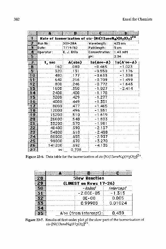
382 Excel for Chemists
480 .1?7 640 ,216 800 .246
1600' .350 . . ., ., ., ., . . ,. ,.. 2400: .4QO 3200. "' .429 4000: .449 8000~ ,477 ,.. _. .., ,, .,. ,. . . . . . . ./,,.. . .
12000: .496 . . ., ., ,.( , 52Q0 .i'o . . . .
26000 .543
Figure 23-6. Data table for the isomerization of cis-[Ni(13aneNq)(H20)2]2+.
Figure 23-7. Results of first-order plot of the slow part of the isomerization of cis-[Ni(13aneNq)(H20)2]2?

Chapter 23 Analysis of Kinetics Data 383
Applying LINEST to the data in the straight-line portion of the slow process (rows 17-26 of Figure 23-6) yields the rate constant for the slow process and permits the calculation of A’, from the intercept value (A0 for the slow process is A, for the fast process). From In (A, - Ao) = -1.315, A, - A0 = 0.269, from which A’-= A0 = 0.439, as shown in Figure 23-7.
Figure 23-8. Results of first-order plot of the fast part of the isomerization of cis-[Ni(13aneNq)(H20)212+.
Having established the value for A’,, the data from the early stages of the reaction can be analyzed as a first-order process by plotting In 1 At - A ‘- 1 (see the inset in Figure 5-23). The results are shown in Figure 23-8.
CONSECUTIVE REVERSIBLE FIRST-ORDER REACTIONS
The sequence of coupled reversible first-order processes
yields the following set of differential equations:
44 t - - - kl [Alt + k2 PI t dt -
d[Bl t - = kl [AIt - k2 IBIt - k3 [Bl t + k4 [cl t dt
d[Cl t - = k3 Pit - k4 Kit dt
The differential equations can be solved to yield analytical expressions for the concentrations of A, B and C. For the case where [B]o = [Cl0 = 0 at t = 0, the
expressions are* :
kl CA2 - k3 - k4,& f, kl (k3 + k4 - A31 &3 t A2 &2- h3) A3 @2 - h3) I
(21-15)
John W. Moore and Ralph G. Pearson, Kinetics and Mechanism, 3rd edition, Wiley- Interscience, New York, 1982, p. 298.

384 Excel for Chemists
Wit = [Alo kl k4 A2 A3 +
h (k4 - h2) e-h2 t +
A2 (A2 - h3)
kl (A3 - k4> e-h3 t
A3 (A2 - h3) 1 kl k3 h k3
Kit = IAl0 h2 h3 +A2 (A2- h3) [ e -A:! t- h k3
A3 (A2 - h3) e--h3 t 1
(23-16)
(23-17)
where A2 = (p + qv
A3 = (P-W p = (kl + k2 + k3+ k4)
q = [p2 + 4(klk3 + k2k4 + k1k4)]1/2
(23-18)
(23-19)
(23-20)
(23-21)
A system such as this can readily be solved by using the Solver. The previous example of the isomerization of cis-[Ni(13aneN4)(H20)2]2+ (Figure 23- 5),is actually a case of coupled reversible first-order processes. There are two observable rate processes, kfast and kslow, but each is reversible. Treatment of the data according to the consecutive reversible first-order scheme is shown in Figure 23-6.
The expressions for [AIt, [B]t , [C]t and Abs,,lc in cells Cl 4, D14, El 4 and F14 are:
=C_T*(k-2*k-4/(Ls2*L-3)+k-1 *(L-2-k-3-k-4)*EXP(-LB2*t)/ L-2*(L-2-L-3))+k-l *(k-3+k-4-L_3)*EXP(-L_3*t)/ (L3*(L2-L3)))
=C-T*(kJ *k-4/(L-2*L-3)+k-l *(k-4-L-2)*EXP(-L_2*t)/ (L-2*(L-2-L-3))+k-l *(L-3-k-4)*EXP(-L-3*t)/(L-3*(L-2-L-3)))
=C-T*(kJ *k~3/(L~2*L~3)+k~l *k~3*EXP(-L~2*t)/(L~2*(L~2-L~3))- k-1 *k-3*EXP(-L-3*t)/(L-3*(L-2-L-3)))
The quantities p, q, h2 and h3 were calculated by using the formulas:
=k l+k 2+k 3+k 4 - - - -
=SQRT(P*P-4*(k-1 *k-3+k-2*k-4+k-l “k-4))
=( P+Q)/2
=( P-Q)/2

Chapter 23 Analysis of Kinetics Data 385
The Solver was used to minimize the sum of squares of residuals (cell G12, Figure 23-9) by changing the values of kl, k2, k3 and k4, and the molar absorptivity of the intermediate species B (EA and EC could be determined separately). The Solver provided a reasonable fit to the data. All five changing cells could be varied at once, although approximate estimates of the parameters had to be provided before the Solver could proceed to a solution. The five parameters of the Solver solution are shown in bold in Figure 23-9.
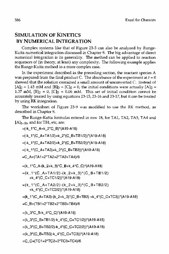
386
SIMULATION OF KINETICS BY NUMERICAL INTEGRATION
Excel for Chemists
Complex systems like that of Figure 23-5 can also be analyzed by Runge- Kutta numerical integration discussed in Chapter 9. The big advantage of direct numerical integration is its generality. The method can be applied to reaction sequences of (in theory, at least) any complexity. The following example applies the Runge-Kutta method to a more complex case.
In the experiment described in the preceding section, the reactant species A was prepared from the final product C. The absorbance of the experiment at t = 0 showed that the solution contained a small amount of unconverted C. Instead of [A]0 = 1.43 mM and [B]o = [C]o = 0, the initial conditions were actually [A]0 = 1.37 mM, [B]o = 0, [Cl0 = 0.06 mM. This set of initial condition cannot be accurately treated by using equations 23-15,23-16 and 23-17, but it can be treated by using RK integration.
The worksheet of Figure 23-9 was modified to use the RK method, as described in Chapter 9.
The Runge-Kutta formulas entered in row 18, for TAl, TA2, TA3, TA4 and [AIt+&, and for TBl, etc, are:
=(-k-l *C_A+k_2*C_B)*(Al g-Al 8)
=(-k-l *(C~A+TA1/2)+k~2*(C~B+TB1/2))*(A19-A18)
=(-k-l *(C-A+TA2/2)+k-2*(C-B+TB2/2))*(A19-A18)
=(-k-l *(C-A+TA3)+k-2*(C_B+TB3))*(Al g-Al 8)
=CAA+(TA1+2*TA2+2*TA3+TA4)/6
=(k-1 *C-A-(k_2+k_3)*C_B+k_4*C_C)*(Al g-Al 8)
=(kJ *(C_A+TA1/2)-(k_2+k_3)*(C_B+TB1/2) +k_4*(C_C+TC1/2))*(Al g-Al 8)
=(k-1 *(CmA+TA2/2)-(k-2+k-3)*(C_B+TB2/2) +k-4*(CsC+TC2/2))*(A19-A18)
=(k-1 *(CmA+TA3)-(k-2+k-3)*(C_B+TB3) +k-4*(CeC+TC3))*(A19-Al 8)
=C B+(TB1+2*TB2+2*TB3+TB4)/6 -
=(k_3*(C_B+TB2/2)-k_4*(C_C+TC2/2))*(Al g-Al 8)
=(k-3*(C-B+TB3)-ks4*(C_C+TC3))*(A1 g-Al 8)
=CsC+(TC1+2*TC2+2*TC3+TC4)/6

Chapter 23 Analysis of Kinetics Data 387
Following the layout suggested in Chapter 9, the initial concentration of A was entered in cell Cl 8; cell Cl 9 contains the formula =H 18. Similar formulas were used for [B]t and [C]t.
When the RK method (or any method involving numerical integration) is used, it is important to chose time increments small enough to assure accuracy in calculations. In the RK formulas above, a calculated time increment, e.g. (A19- A18) in row 18, was used rather than a constant value, so that the interval between successive data points could be varied. In this way larger time increments can be used at the end of the reaction, when concentrations are changing slowly. Only a few cells in column B contain A&d measurements; only one is shown in the spreadsheet fragment of Figure 23-10. The data table of time and A,bsd values was located elsewhere in the worksheet; VLOOKUP was used in column B to enter the A,bsd values for the appropriate time values. The formula is as follows:
=IF(ISERROR(VLOOKUP(t,DataTable,l ,O)),““,VLOOKUP(t,DataTable,2,0))
The ISERROR function was used with range-lookup = 0; otherwise VLOOKUP returns #N/A! for all values of t for which there is no corresponding entry in DataTable.
An IF statement was used to calculate the squares of residuals only for rows that contained an A&d value.
The Solver was used in the same way as in the preceding example, although it was necessary to use subsets of the complete set of parameters to perform the initial stages of the refinement. Note the difference in the results when the small amount of product species that was present at the beginning of the reaction is taken into acount: the values of the regression parameters are significantly different, and the sum of squares of residuals (1.38 x lOA) is significantly smaller than in the preceding treatment (4.52 x 10⁴).
Calculation time will be significantly longer for a solution by direct numerical integration than for a solution using analytical expressions.

388 Excel for Chemists
k-l = : 4,34E-04
small 3mountofC present: [C]i=
Moe .f% EA= E-b= ,.. .,. ,., ,.,.
. . . . E*=
. . . . . . .,
1.37E-03' ..,. . . ,.,.,I 6 .##E-05
+A2 ‘. -5.92E-06 -5.87E-06 :=j ,#iE-&
-5.77E-#i -5.72E-06 -5.6%‘0i -5.62E-06 -5.57E-06 -l.l#E-05 -l.WE-05 -l.WE-05 - j, .04ET05 -2.03E-05 -1.96E-05
Figure 23-10. Data table for the isomerization of cis-[Ni(13aneNq)(H20)2]2+ analyzed by the RK method. Columns I through Y (not shown) contain formulas for calculation of [B] and [Cl.

APPENDICES
Excel for Chemists: A Comprehensive Guide. E. Joseph BilloCopyright 2001 by John Wiley & Sons, Inc.
ISBNs: 0-471-39462-9 (Paperback); 0-471-22058-2 (Electronic)

A SELECTED WORKSHEET FUNCTIONS
BY CATEGORY
Excel 2000 provides more than 300 worksheet functions, in 11 categories: Engineering, Financial, Date & Time, Information, Math & Trig, Statistical, Lookup & Reference, Database, Text, Logical, External. This book uses functions from seven of those categories. This appendix lists selected worksheet functions by category. In Appendix B, the functions are listed alphabetically, with comments, examples and related functions.
DATABASE & LISTMANAGEMENT FUNCTIONS DAVERAGE Returns the average of selected values. DCOUNT Returns the number of cells that contain numbers in a
specified field, according to specified criteria. DCOUNTA Returns the number of cells that contain values in a
specified field, according to specified criteria. DGt Returns a single record that matches the specified
criteria. DMAX Returns the maximum value in the range Database. DMIN Returns the minimum value in the range Database. DPRODUCT Returns the product of values in a specified field that
match specified criteria in a database. DSTDEV Returns the standard deviation of values in a specified
field that match specified criteria in a database. DSTDEVP Returns the standard deviation of values in a specified
field that match specified criteria in a database. DSUM Returns the sum of numbers in the field column of
records in the database that match the criteria. DVAR Returns the variance of values in a specified field that
match specified criteria in a database. DVARP Returns the variance of values in a specified field that
match specified criteria in a database. SUBTOTAL Returns a subtotal in a database.
391
Excel for Chemists: A Comprehensive Guide. E. Joseph BilloCopyright 2001 by John Wiley & Sons, Inc.
ISBNs: 0-471-39462-9 (Paperback); 0-471-22058-2 (Electronic)

392 Excel for Chemists
DATE & TIME FUNCT..ONS DATE Returns the serial number of a date. DATEVALUE Converts a date in the form of text to a serial number. DAY Converts a serial number to a day of the month. MONTH Converts a serial number to a month.
Returns the serial number of the current date and time. TODAY WEEKDAY YEAR
Returns the serial number of today’s date. Converts a serial number to a day of the week. Converts a serial number to a year.
INFOWATION FUNCTIONS CELL Returns information about the formatting, location or
contents of a cell. COUNTBLANK ERRORJYPE INFO
Counts the number of blank cells within a range. Returns a number corresponding to an error value. Returns information about the current operating environment.
ISBLANK ISERR
Returns TRUE if the cell is blank. Returns TRUE if the argument is any error value except #N/A.
ISERROR ISEVEN ISLOGICAL ISNA ISNONTEXT ISNUMBER ISODD ISREF ISTEXT N
NA TYPE
Returns TRUE if the argument is an error value. Returns TRUE if the argument is even. Returns TRUE if the argument is a logical value. Returns TRUE if the argument is # N/A. Returns TRUE if the argument is not text. Returns TRUE if the argument is a number. Returns TRUE if the argument is odd. Returns TRUE if the argument is a reference. Returns TRUE if the argument is text. Returns a value converted to a number. Excel usually does this automatically when necessary. Returns the error value #N/A Returns a number indicating the data type of a value.
LOGICAL FUNCTIONS AND Returns TRUE if all arguments are true, otherwise FALSE< FALSE Returns the logical value FALSE. IF Returns one value if logical test is TRUE, another value -
if logical test is FALSE. - NOT Reverses the logic of its argument.
CR Returns TRUE if any argument is TRUE. TRUE Returns the logical value TRUE.

Appendix A Selected Worksheet Functions by Category 393
LOOKUP &REFERENCE FUNCTlIONS ADDRESS Returns a reference in the form of text. AREAS Returns the number of areas in a multiple selection.
Chooses a value from a list of values, based on index number.
COLUMN Returns the column number of a reference. COLUMNS Returns the number of columns in a reference. HLOOKUP Finds the value in the first row of an array that is equal
to or less than lookup - value. Returns the associated value in the nth row, as determined by offset-gum. Returns a value from a reference or array, using a specified index. Returns a reference specified by a text value. Looks up values in an array. Looks up a value in an array and returns its relative position. Returns a reference offset from a base reference by specified number of rows and columns. Returns the row number of a reference. Returns the number of rows in a reference. Returns the transpose of an array. Finds the value in the first column of an array that is equal to or less than lookup-value. Returns the associated value in the nth column, as determined by
INDEX
INDIRECT LOOKUP MATCH
OFFSET
TRANSPOSE VLOOKUP
offset-num.
A4AT.H G, TRIG FUNCT..ONS ABS Returns the absolute value of a number. ACOS Returns the angle corresponding to a cosine value. ACOSH ASIN ASINH ATAN ATAN
ATANH
COUNTIF
DEGREES EXP
Returns the inverse hyperbolic cosine of a number. Returns the angle corresponding to a sine value. Returns the inverse hyperbolic sine of a number. Returns the angle corresponding to a tangent value. Returns the angle defined by a pair of x- and y coordinates. Returns the inverse hyperbolic tangent of a number. Returns the cosine of a given angle. Returns the hyperbolic cosine of a number. Returns the number of non-blank cells within a range that meet the given criteria. Converts a value in radians to degrees. Returns the value of e raised to the power number.

394 Excel for Chemists
FACT INT LN
LOG10 MDETERM MINVERSE MMULT
MROUND PI PRODUCT RADIANS RAND RANDBEWVEEN ROMAN ROUND ROUNDDWN ROUNDUP SIGN SIN SINH SQRT SUM SUMIF
SUMPRODUCT
SUMSQ TAN TANH TRUNC
Returns the factorial of a number, i. e., 1*2*3*... number. Rounds a number down to the nearest integer. Returns the base-e logarithm of a number. Returns the logarithm of a number to the specified base. Returns the base-10 logarithm of a number. Returns the determinant of an array. Returns the inverse of an matrix . Returns the product of two matrices. Returns the remainder of the division of number by divisor. Returns a number down to the nearest specified level. Returns nl. Returns the product of the specified arguments. Converts an angle in degrees to radians. Returns a random number between 0 and 1. Returns a random number within a specified range. Converts an Arabic number to Roman numerals. Rounds a number to a specified number of digits. Rounds a number down. Rounds a number up. Returns the sign of a number. Returns the sine of a given angle. Returns the hyperbolic sine of a number. Returns the square root of a number. Returns the sum of all the numbers in the reference. Returns the sum of all the numbers in the reference that satisfy the specified criteria. Returns the sum of the products of corresponding array components. Returns the sum of the squares of arguments. Returns the tangent of a given angle. Returns the hyperbolic tangent of a number. Truncates a number.

Appendix A Selected Worksheet Functions by Category 395
STATISTICAL FUNCTIONS AVEDEV
AVERAGE CORREL COUNT COUNTA
INTERCEPT
LARGE LINEST MAX MEDIAN MIN PEARSON SLOPE SMALL STDEV VAR
TEXT FUNCTIONS CHAR
CLEAN
CONCATENATE DOLLAR EXACT
FIND
FIXED
LEFr
MID
PROPER
Returns the average absolute deviation of data points from the mean. Returns the average of all the numbers in the reference. Returns the correlation coefficient between two data sets. Returns the number of numbers in the reference. Returns the number of non-blank values in the reference. Returns the intercept of the linear regression line y=mx+b. Returns the kth largest value in a list of values. Returns the parameters of multiple linear regression. Returns the maximum value in a list of arguments. Returns the median value in a list of arguments. Returns the minimum value in a list of arguments. Returns the Pearson correlation coefficient. Returns the slope of the linear regression line y = mx + b.. Returns the kth smallest value in a list of values. Returns the standard deviation of a sample. Returns the variance of a sample.
Returns the character corresponding to the character code number. Removes all non-printable characters from a text string. Returns the numeric code corresponding to a character. Concatenates text values into a single text string. Converts a number to a text value in currency format. Compares two text strings; returns TRUE if they are the same. Returns the position at which one text string occurs within another text string. Rounds a number to the specified number of decimal places and returns the result as text. Returns the specified number of characters from a text string, beginning at the left. Returns the number of characters in a text string. Converts a text string to lowercase. Returns the specified number of characters from a text string, beginning at the specified position. Capitalizes the first letter in each word of a text string.

396 Excel for Chemists
REPLACE
REW- RIGHT
SEARCH SUBSTITUTE
T
TEXT TRIM
UPPER VALUE
Replaces characters at a specified position within a text string. Repeats Returns
a text value a specified number of times. the specified number of characters from a text
string, beginning at the right. Finds the position of a text value within a text string. Finds and substitutes characters within a text string.
Converts a value to text. Excel usually does this automatically when necessary. Formats a number and returns it as text. Removes spaces from a text string, except for single spaces between words. Converts a text string to uppercase. Converts a text argument to a number. Excel usually does this automatically when necessary.

B ALPHABETICAL LIST OF
SELECTED WORKSHEET FUNCTIONS
This appendix lists selected worksheet functions that will be useful in creating advanced worksheet formulas for chemical applications. For each function, a description of the function and its syntax are given; most cases include an example of the use of the function, and any related functions are listed. Function arguments are in italics; arguments are in boldface type if the argument is required and plain text if the argument is optional. The required data type for an argument is indicated by the suffixes JW~, -ref, - logical, - text. If a function can accept an argument of more than one type, then no suffix is attached.
ABS Returns the absolute value of a number Syntax: ABS(number) Example: =ABS(-7.3) returns 7.3 Related Function: S I G N
ACOS Returns the angle corresponding to a cosine value. Syntax: ACOS(number) Number must be from -1 to +l. The returned angle is in radians, in the range 0 to n;. To convert the result to degrees, multiply by 180/n. Example: =ACOS(O) returns 1.570796327, or 90 degrees. Related Functions: COS, other trigonometric functions
ADDRESS Returns a reference in the form of text. Syntax: ADDRESS(row_num,column_num,abs_num,aI,sheet_text) Abs num specifies the type of reference to return. If abs-num is 1 or omitted, - returns an absolute reference; if 2, absolute row and relative column; if 3, relative row and absolute column; if 4, relative. Al is a logical value that specifies the A 1 or Rl Cl reference style. If Al is TRUE or omitted, ADDRESS returns an Al-style
397
Excel for Chemists: A Comprehensive Guide. E. Joseph BilloCopyright 2001 by John Wiley & Sons, Inc.
ISBNs: 0-471-39462-9 (Paperback); 0-471-22058-2 (Electronic)

398 Excel for Chemists
reference; if FALSE, ADDRESS returns an RI Cl -style reference. Sheet-text is text specifying the name of the worksheet to be used as the external reference. If sheet-text is omitted, no sheet name is used. Examples:
=ADDRESS(2,3) returns “$C$2” =ADDRESS(2,3,2) returns X$2” =ADDRESS(2,3,2,FALSE) returns “R2C[3]” =ADDRESS(2,3,1 ,FALSE,“[Bookl]Sheetl “) returns “[Bookl]Sheetl !R2C3” c
Relafed Functions: COLUMN, INDIRECT, ROW
AND Returns TRUE if all arguments are TRUE, otherwise returns FALSE. Syntax: AND(/ogica/l,/ogica/Z,...) Up to 30 logical conditions can be tested. Example= If Al contains 0 and A2 contains 1 IO, then =AND(Al =O,A2>100) returns TRUE. Relafed Functions: NOT, OR
AREAS Returns the number of areas in a multiple selection. Syntax: AREAS(reference) Related Functions: COLUMN, COLUMNS, ROW, ROWS
ASIN Returns the angle corresponding to a sine value. Syntax: ASIN(number) Number must be from -1 to +l. The returned angle is in radians, in the range -z/2 to +n;/2. To convert the result to degrees, multiply by 180/z Example: If AI contains 0.7071, then =ASIN(Al) returns 0.785388573, or 45 degrees. Related Functions: SIN, other trigonometric functions
ATAN Returns the angle corresponding to a tangent value. Syntax: ATAN(number) The returned angle is in radians, in the range 0 to 7~. To convert the result to degrees, multiply by 180/n. Example: =ATAN(O) returns 0.785388573 or 45 degrees. Related Functions: ATAN2, TAN, other trigonometric functions
ATAN Returns the angle defined by a pair of x- and y coordinates. The angle is between the x axis and the line connecting the origin (0,O) and the point (x,y). Syntax: ATAN2(x_num,y_num) The returned angle is in radians, in the range -n: to 7~. To convert the result to

Appendix B Alphabetical List of Selected Worksheet Functions 399
degrees, multiply by 180/n;. A negative result represents a clockwise angle from the x-axis. Example: =ATAN2(3,4) returns 0.927295218, or 53.13 degrees. Related Funcfions: ATAN, TAN, other trigonometric functions
AVERAGE Returns the average of all the numbers in the reference. Syntax: AVERAGE(numberl,numberZ,...) The arguments may be numbers, or names, arrays or references that contain numbers. Up to 30 separate arguments can be listed. Only numbers in the array or range are counted. Related Funcfion: M E D I AN
CELL Returns information about location, formatting and contents of a cell. Synfax: CELL(info-type-text,reference) info - type - text specifies the cell information to be returned. If reference is omitted, information about the active cell is returned. For further information, see Microsoft Excel 97 Worksheet Function Reference. Example: If the cell format is O.OOE+OO, =CELL(“format”) returns S2. Related Function: I N FO
CHAR Returns the character corresponding to the character code number, in either the Macintosh character set or the ANSI character set (Windows). Syntax: CHAR(nomber) Number must be between 1 and 255. Example: =CHAR(65) returns A. Related Function; C 0 D E
CHOOSE Chooses a value from a list of values, based on index number. Syntax: CHOOSE(index number, va/ueI,va/ueZ,...) index number must be a number between 1 and 29, or a formula or reference that - evaluates to same. The arguments may be numbers, names, formulas or references. Example: If cell H8 contains 1, then =CHOOSE(H8+1 ,$F$2,$G$2,$H$2,$1$2)/SUM($F$2:$1$2) calculates the fraction $G$2/SUM($F$2:$1$2). Related Functions: INDEX, MATCH
CLEAN Removes all non-printable characters from a text string. Syntax: CLEAN(text) Use on text imported from other applications that may contain non-printing

400 Excel for Chemists
characters. Related Function: T R I M
CODE Returns the numeric code for the first character of text, Syntax: CODE( text) Example: =CODE (“A”) returns 65. Related Function: C H A R
COLUMN Returns the column number of reference. Syntax: COLUMN(reference) If reference is a range of cells, returns the column number of the upper left cell of the range. Reference cannot be a multiple selection. If reference is omitted, it is assumed to be the reference in which the COLUMN function appears. Example: If C3:NlO is selected, then =COLUMN(SELECTlON()) returns 3. Related Functions: COLUMNS, ROW, ROWS
COLUMNS Returns the number of columns in reference. Syntax: COLUMNS(reference) If reference is a multiple selection, use INDEX to select a specified area within the selection. Example; If C3:NlO is selected, then =COLUMNS(SELECTlON()) returns 12. Related Functions: COLUMN, ROW, ROWS
CORREL Returns the correlation coefficient between two data sets. Syntax: CORREL(arrayI,arrayZ) Array7 and array2 must have the same number of data points. Related Functions: SLOPE, INTERCEPT, COVAR, PEARSON, RSQ
Returns the cosine of a given angle. Syntax: COS(number) Number is the angle in radians. To convert an angle in degrees to one in radians, multiply by n/180. Related Functions: ACOS, SIN, TAN, other trigonometric functions
COUNT Returns the number of numbers in the list or range. Syntax: COUNT( va/ueI,va/ue2,...) Up to 30 arguments are allowed. Any value, other than an empty cell, is counted. Related Functions: COUNTA, COUNTBLANK, COUNTIF

Appendix B Alphabetical List of Selected Worksheet Functions 401
COUNTA Returns the number of non-blank values in the list or range. Syntax: COUNTA( va/ueI,va/ueZ,...) Up to 30 arguments are allowed. Nulls (““), logical values, numbers formatted as dates, or text values that can be converted to numbers, are counted. Related Functions: COUNT, COUNTBLANK, COUNTIF
COUNTBLANK Returns the number of blank cells within a range. Sy~~fax: COUNTBLANK(reference) Cells containing null values are counted, but cells containing zero values are not counted. Relafed Funcfions: COUNT, COUNTA, COUNTIF
COUNTIF Returns the number of cells within a range that meet the specified criteria. Syntax: COUNTI F( reference,criferia) Example; =COUNTIF(year_of_graduation,c1990) Related Functions: COUNT, COUNTA, COUNTBLANK, SUMIF
DATE Returns the serial number of a particular date. Syntax: D AT E ( year, month, day) Year is a number from 1900 (Windows) or 1904 (Macintosh) to 9999. Year can be specified using two digits if in the range 1920 to 2019; otherwise use four digits. Month or day can be greater than 12 or 31 (see example). Example: DATE(94,7,4) corresponds to July 4, 1994. DATE(94,7,90) corresponds to Sept. 28,1994. Relafed Funcfions: DATEVALUE, DAY, MONTH, YEAR, NOW, TODAY
DATEVALUE Converts a date in the form of text to a serial number. Syntax: DATEVALUE( fexf) Example: =DATEVALUE(“3 Aug 1938”) returns 12633 if the 1904 Date System is in effect. Relafed Functions: NOW, TODAY
DAY Converts a serial number to a day of the month. Syntax: DAY (serial-number) SeriaLnumber can also be given as text, such as “Jul-4-1994”. Returns a value in the range 1 to 31. Related Funcfions: NOW, TODAY, WEEKDAY, YEAR, MONTH

402 Excel for Chemists
DEGREES Converts an angle in radians to degrees Syntax: DEGREES(number) Available in Excel 4.0 only as an add-in function. Related Functions: RADIANS, trigonometric functions
EXACT Compares two text strings; returns TRUE if they are the same. Syntax: EXACT( textl,text2) EXACT is case-sensitive. Related Functions: FIND, SEARCH
EXP Returns the value of e raised to a power. Syntax: EXP(number) Returns the value of e raised to the power number. Related Functions: LN, LOG
FACT Returns the factorial of a number. Syntax: FACT(number) Returns the factorial of a number, i.e., 1*2*3*...ntrmbeu. Number must be positive. If number is not an integer, it is truncated.
FIND Returns the position at which one text string occurs within another text string. Syntax: F I N D ( find - text, within- text, start-number) Find text is the text string you want to find. - Within text is the string you are - searching. Start-number is the character at which to start searching. If start_number is omitted, it is assumed to be 1. FIND is case-sensitive. Example: If cell A3 contains BILLO, E JOSEPH, the formula =FIND(“,“,A3) returns 6. Related Functions: EXACT, SEARCH
FIXED Rounds a number to the specified number of decimal places and returns the result as text. Syntax: FIXED( number, decimals, no-commas-flag) Number is the number to be converted. Decimals is the number of decimal places desired; if decimals is omitted, it is assumed to be 2. If decimals is negative, number is rounded to the left of the decimal point. If no commas flag is TRUE, - - commas are not included in the formatted number. Example: =FIXED( 12345,3,1) returns 12345.000. =FIXED( 12345) returns 12,345.OO. =FIXED( Pl(),4) returns 3.1416. Related Functions: ROUND, TEXT

Appendix B Alphabetical List of Selected Worksheet Functions 403
HLOOKUP Finds the value in the first row of an array that is equal to or less than lookup-value. Returns the associated value in the nth row, as determined by offset-num. Syntax: H LOOKU P( lookup - value, array, offset-num, match-logical) The values in the first row must be in ascending order. If match_logica/ is TRUE or omitted, returns the largest value that is less than or equal to lookup value. If - match-/ogica/is FALSE, returns #N/A if an exact match is not found. Example: See example under VLOOKUP. Related Functions: INDEX, MATCH, VLOOKUP
IF Returns one value if logical - test is TRUE, another value if logical test is FALSE. Syntax: IF(/ogica/ test, value-if- TRUE, value-if- FALSE) Value if TRUE and/or value if FALSE can be IF functions; up to seven IF functi&an be nested. - - Example: =IF(result=O, O.O8*estimate, O.O8*result) Related Functions: AND, NOT, OR, IS functions
INDEX Chooses a value from an array, based on row and column number pointers. Syntax: INDEX(array, row-number, column-number) If the array is one-dimensional, only one pointer argument need be specified. Example: If the reference $C$2:$C$lO2 contains the atomic weights of the elements, arranged in order of atomic number, then =INDEX($C$2:$C$102,51) returns the atomic weight of element number 51. Related Functions: CHOOSE, HLOOKUP, MATCH, VLOOKUP
INDIRECT Returns a reference specified by a text string. Syntax: I N D I R ECT(reference- text,A I-logical) Reference text can be an Al - or Rl Cl -style reference, or a name. A I-logical - specifies the form of reference text: if reference text is TRUE or omitted, - - reference-text is interpreted as an Al -style reference; if reference-text is FALSE, reference text is interpreted as an RI Cl -style reference. Example; If ce?l B3 contains “Sheet2!AS” then the formula =INDIRECT(B3) displays the contents of Sheet2!A5. Related Functions: OFFSET
INFO Returns information about the operating environment. Syntax: I N FO( type- text) Type - text specifies what information is to be returned. Some useful values of type - text: “directory” returns path of the current directory or folder, “memavail”
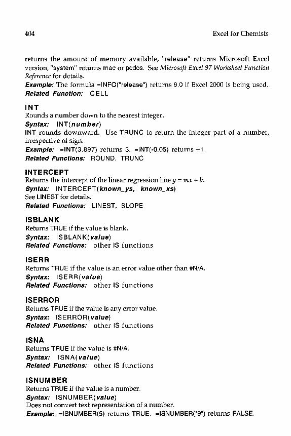
404 Excel for Chemists
returns the amount of memory available, “release” returns Microsoft Excel version, “system” returns mat or pcdos. See Microsoff Excel 97 Worksheet Function Reference for details. Example: The formula =INFO(“release”) returns 9.0 if Excel 2000 is being used. Related Function: C E L L
INT Rounds a number down to the nearest integer. Syntax: INT(number) INT rounds downward. Use TRUNC to return the integer part of a number, irrespective of sign. Example: =INT(3.897) returns 3. =INT(-0.05) returns -1. Related Functions: ROUND, TRUNC
INTERCEPT Returns the intercept of the linear regression line y = mx + b. Syntax: INTERCEPT(known-ys, known-xs) See LINEST for details. Related Functions: LINEST, SLOPE
ISBLANK Returns TRUE if the value is blank. Syntax: ISBLANK( value) Relafed Functions: other IS functions
ISERR Returns TRUE if the value is an error value other than #N/A. Syntax: I S E R R ( value) Related Functions: other IS functions
ISERROR Returns TRUE if the value is any error value. Syntax: lSERROR( value) Related Functions: other IS functions
ISNA Returns TRUE if the value is #N/A. Syntax: ISNA( value) Relafed Functions: other IS functions
ISNUMBER Returns TRUE if the value is a number. Syntax: I S N U M B E R ( value) Does not convert text representation of a number. Example: =ISNUMBER(S) returns TRUE. =ISNUMBER(“SI’) returns FALSE.

Appendix B Alphabetical List of Selected Worksheet Functions 405
Related Functions: other IS functions
ISTEXT Returns TRUE if the value is text. Syntax: ISTEXT( value) Related Functions: other IS functions
LARGE Returns the kth largest value in a list of values. Syntax: LARGE(array,k) Related Funcfions: MAX, MIN, SMALL
LEFT Returns the specified number of characters from a text string, beginning at the left Syntax: L E FT( text, nwn~chars) If num chars is omitted, it is assumed to be 1. - Example: =LEFT(“CHEMlSTRY”,4) returns CHEM. Related Fundions: LEN, MID, RIGHT
LEN Returns the number of characters in a text string. Syntax: LEN(text) Example: =LEN(“CHEMISTRY”) returns 9. Related Functions: LEFT, MID, RIGHT
LINEST Returns an array of linear regression parameters. Syntax: LINEST(known-ys, known-xs, const-logical, stats-logical) See Chapter 11 for details. Related Functions: CORREL, INTERCEPT, SLOPE
LN Returns the natural (base-e) logarithm of a number. Syntax: LN(number) Related Functions: EXP, LOG
LOG Returns the logarithm of a number to the specified base. Syntax: LOG(number, base) If base is omitted, returns the base-10 logarithm. Related Functions: LN, LOG1 0
LOG10 Returns the base-10 logarithm of a number. Syntax: LOG 1 0( number)

406 Excel for Chemists
Related Functions: LN, LOG
LOOKUP Looks up a value in an array. The LOOKUP function has two syntax forms: vector and array. The vector form of LOOKUP looks in a one-row or one-column range for a value and returns a value from the same position in a second one-row or one-column range. See the On- line Help for information about the array form of LOOKUP. Syntax: LOOKUP(lookup~value,/ookup~vector,resu/t~vector) The values in lookup - vector must be placed in ascending order; if LOOKUP can’t find the lookup - value, it matches the largest value in lookup vector that is less - than or equal to lookup value. Related Functions; HLOOKUP, MATCH, VLOOKUP
LOWER Converts a text string to lowercase. Syntax: LOWE R ( text) Related Functions: PROPER, UPPER
MATCH Looks up a value in an array and returns its relative position. Syntax: M ATC H ( lookup value, array, match type) If match- type = 0, the fun&ion finds the first value that is exactly equal to lookup - value; array can be in any order. If match type = 1, finds the largest - value that is less than or equal to lookup-value; array must be in ascending order. If match-type = -1, finds the smallest value that is greater than or equal to lookup - value; array must be in descending order. Example: =MATCH(MAX(Spectrum),Spectrum,O) returns the relative position in the array Spectrum of the maximum value in the array. Related Functions: HLOOKUP, INDEX, VLOOKUP
MAX Returns the maximum value in a list of arguments. Syntax: MAX( numberl, numberz,...) There may be up to 30 arguments. If an argument is a reference, only numbers in the reference are examined. Related Function: M I N
MDETERM Returns the determinant of an array. Syntax: MDETERM(array) Array must have an equal number of rows and columns. If any cells in array do not contain numbers, returns #VALUE!. Example: See Chapter 9 for details. Related Functions: MINVERSE, MMULT, SUMPRODUCT, TRANSPOSE

Appendix B Alphabetical List of Selected Worksheet Functions 407
MEDIAN Returns the median value in a list of arguments. Syntax: MEDIAN(number7, number&...) If there are an even number of numbers in the set, returns the average of the two median values. Relafed Function: AVERAGE
MID Returns the specified number of characters from a text string, beginning at the specified position. Syntax: MlD(text, startgum, num-chars) If num chars extends beyond the end of text, returns characters to the end of text. - Example: If cell A4contains H2S04, =MID(A4,2,1) returns 2. Related Functions: LEFT, LEN, RIGHT
MIN Returns the minimum value in a list of arguments. Syntax: MIN(number7, numberZ,...) There may be up to 30 arguments. If an argument is a reference, only numbers in the reference are examined. Related Function: M A X
MINVERSE Returns the inverse of a matrix. Syntax: MINVERSE(array) Array must have an equal number of rows and columns. If any cells in array do not contain numbers, MINVERSE returns #VALUE!. If MDETERM for the array returns 0, the array cannot be inverted; MINVERSE will return #NUM! error. Example: See Chapter 9 for details. Related Functions: MDETERM, MMULT, SUMPRODUCT, TRANSPOSE
MMULT Returns the product of two matrices. Syntax: M M U LT( arrayl, array2) COLUMNS for array7 must equal ROWS for array2. Example: See Chapter 9 for details. Related Functions: MDETERM, MINVERSE, SUMPRODUCT, TRANSPOSE
MOD Returns the remainder of the division of number by divisor. Syntax: M 0 D ( number, divisor) If divisor is greater than number, returns number. Use MOD(number,l) to return the decimal part of a floating-point number. Example: =MOD(2.3333,2) returns 0.3333. =MOD(2.3333,3) returns

408 Excel for Chemists
2.3333. =MOD(I 0.37,1) returns 0.37. Related Functions: INT, ROUND, TRUNC
MONTH Converts a serial number to a month. Syntax: MONTH(seria/-number) Seria/-number can also be given as text, such as “Jul-4-1994”. Returns a number between 1 and 12. Related Functions: YEAR, DAY, WEEKDAY
NA Returns the error value #N/A Synfax: N A ()
NOT Reverses the logical value of its argument. Syntax: NOT( logical) Example: =IF(NOT(ISERROR(F2/G2)),F2/G2,““) Related Functions: AND, OR
NOW Returns the serial number of the current date and time. Syntax: NOW0 The integer part of the serial number represents the day, month and year; the decimal part represents the time. NOW is recalculated whenever the sheet is recalculated. Related Functions: DATE, TODAY, YEAR, MONTH, DAY
OFFSET Returns a reference offset from a base reference by specified number of rows and columns. Syntax: 0 F F S ET ( reference, rows, co/s, height, width) Rows or columns can be negative. Height and width must be positive. If height and width are omitted, they are assumed to be the same as in reference. Example: =OFFSET(table, rows, cols, 1 ,I) returns a reference to a single cell within the reference tab/e. Related Function: I N D E X
OR Returns TRUE if any argument is TRUE. Syntax: OR(/ogica/l, IogicalZ,...) Up to 30 logical conditions can be tested. Example: If cell G2 contains 0.75, the formula =IF(OR(G2<=O,G2>=1),““, F2/G2) returns 1.33333333; if cell G2 contains 1.75, the formula returns a null.

Appendix B Alphabetical List of Selected Worksheet Functions 409
Relafed Functions: AND, NOT
PEARSON Returns the Pearson product moment correlation coefficient between two data sets. Syntax: PEARSON(array7, array2) Array1 is the array of independent (x) values; array2 is the array of dependent (y) values. Returns a value of R between -1 and 1. Example: See Microsoft Excel 97 Worksheet Function Reference for details. Related Functions.= CORREL, RSQ
PI Returns 7~. Syntax: P I ()
PRODUCT Returns the product of the specified arguments. Syntax: PRODUCT(numberl,numberZ,...) Up to 30 numbers can be multiplied. Related Function: S U M
PROPER Capitalizes the first letter in each word of a text string. Syntax: P R 0 P E R ( text) Example: =PROPER(“JOHN Q. PUBLIC”) returns John Q. Public. Related Funcfions: LOWER, UPPER
RADIANS Converts an angle in degrees to radians. Syntax: RADIANS(number) Available in Excel 4.0 only as an add-in function. Related Functions: DEGREES, trigonometric functions
RAND Returns a random number between 0 and 1. Syntax; RAND0 A new random number is generated each time the worksheet is recalculated. You may need to Copy and Paste Special (Values) to prevent a random-number series from changing each time you change anything on a worksheet. Example: =O.l*(05RAND()) returns a number between -0.05 and +0.05.
REPLACE Replaces characters at a specified position within a text string. Syntax: R E PLAC E (o/d text, start-num, num-chars, new-text) Old-text is the text in which characters are to be replaced. Start-num is the position of the first character in old-text to be replaced. Num-chars is the

410 Excel for Chemists
number of characters to be replaced. New-text is the text to replace characters in old- text. Example= If cell Al contains the text General Chemistry I Lab, the formula =REPLACE(Al ,19,1 ,“ll”) returns General Chemistry II Lab. Related Functions: SEARCH, SUBSTITUTE
REPT Repeats a text string a specified number of times. Syntax: R E PT( texf, number) Example: If decimals = 3, the formula =“O.“&REPT(“O”,decimals) returns 0.000 as text.
RIGHT Returns the specified number of characters from a text string, beginning at the right. Syntax: R I G HT( text, num_chars) If num chars is omitted, it is assumed to be 1. - Example: =RIGHT(303585842,4) returns 5842. Relafed Functions: MID, LEFT, LEN
ROMAN Converts an Arabic number to Roman numerals. Syntax: ROMAN(number, form) If form = 0, TRUE or omitted, the “classic” form is returned. Form can also be 1,2, or 3, in which case successively more “concise” forms are returned. If form = 4 or FALSE, a “simplified” form is returned. Example: =ROMAN(1997,0) returns MCMXCVII.
ROUND Rounds a number to a specified number of digits. Syntax: R 0 U N D (number, digits) If the result ends in a zero, the zero is not displayed. Example: If cell Al contains 0.001736, the formula =ROUND(A1,5) returns 0.00174. If cell Al contains 0.007702, the same formula returns 0.0077, i.e., the number is not padded out with trailing zeros. Related Functions: INT, TRUNC, TEXT
ROW Returns the row number of reference. Syntax: ROW (reference) If reference is a range of cells, returns the row number of the upper left cell of the range. Reference cannot be a multiple selection. Example: =ROW(B5:C7) returns 5. Related Functions: COLUMN, ROWS

Appendix B Alphabetical List of Selected Worksheet Functions
ROWS Returns the number of rows in reference. Syntax: ROWS(reference) If reference is a multiple selection, can use the selection. Example: =ROWS(BS:C7) returns 3. Related Functions: ROW, COLUMNS
RSQ Returns the correlation coefficient X2. Syntax: RSQ(known-ys, known-xs)
411
INDEX to select a specified area within
This is the correlation coefficient returned by LINEST. For more details, see LINEST. Related Functions: LINEST, CORREL
SEARCH Finds the position of a text value within a text string. Syntax: SEARCH(find text, within- text, start-num) Find text is the text to be found. Include the ? wildcard character in find text to - - match any single character or * to match any sequence of characters within the source string within- text. Start-num is the position in within-text to begin searching. SEARCH is not case-sensitive, FIND is case-sensitive. Example= See example under FIND. Related Functions: FIND, REPLACE, SUBSTITUTE
SIGN Returns the sign of a number. Syntax: SIGN(number) Returns 1, 0, -1 if the number is positive, zero or negative, respectively. Related Function: A B S
SIN Returns the sine of a given angle. Syntax: SIN(number) Number is the angle in radians. To convert an angle in degrees to one in radians, multiply by n;/180. Related Functions: ASIN, COS, TAN, other trigonometric functions
SLOPE Returns the slope of the linear regression line y = mx + b. Syntax: SLOPE(known-ys, known-xs) See LINEST for details. Related Functions: INTERCEPT, LINEST

412 Excel for Chemists
SMALL Returns the kth smallest value in a list of values. Syntax: SMALL(array,k) Related Functions: LARGE, MAX, MIN
SQRT Returns the square root of a number. Syntax: SQRT(number)
STDEV Returns the standard deviation of a sample. Syntax: STD EV( value I, valueZ,...) The sample can consist of up to 30 separate arguments or arrays. Related Functions: AVERAGE, AVDEV
SUBSTITUTE Finds and substitutes characters within a text string. Syntax: SUBSTITUTE(text, old text, new text, instance num) Text is the string in which character&e to be substituted.
- Old text is the text to -
be replaced. New text is the text to replace old text. - - instance num specifies - which occurrence of old text is to be replaced; if omitted, all are replaced. Example: =SUBSTITUiiE(A3,” “,““,2) replaces the second occurrence of a space in the string in cell A3 with a null . Related Function: R E P LAC E
SUM Returns the sum of all the numbers in the reference. Syntax: SUM(number7, numberZ,...) The arguments may be numbers, names, arrays or references that contain numbers. Up to 30 separate arguments. Only numbers in the array or range are counted. Related Functions: AVERAGE, COUNT, COUNTA
SUMIF Returns the sum of all the numbers in the reference that satisfy the specified criteria. Syntax: S U M I F ( range, criteria, sum-range) Range is the range of cells in which criteria will be evaluated. Sum - range contains the cells that will be summed. If sum-range is omitted, cells in range are summed. Example: =SUMIF(B3:B553,>100,D3:D553) Related Functions: AVERAGE, COUNT, COUNTA
SUMPRODUCT, Returns the sum of the products of corresponding array components. Syntax: SUMPRODUCT(array7, array&..)

Appendix B Alphabetical List of Selected Worksheet Functions 413
Up to 30 arrays may be included. All arrays must have the same dimensions. Related &mctions: MMULT, TRANSPOSE
TAN Returns the tangent of a given angle. Syntax: TAN(number) Number is the angle in radians. To convert an angle in degrees to one in radians, multiply by n/180. Related Functions: ATAN, ATAN2, other trigonometric functions
TEXT Formats a number and returns it as text. Syntax: TEXT( value, format text) Format-text is a number format, sr&lar to those in the Number format dialog box. TEXT converts a number to text; the result will sometimes fail to be calculated as a number. Example: The formula =TEXT(PI(),“O.OOO”) in cell Bl returns 3.142. The formula =2*Bl returns 6.284, but the formula =SUM(Bl) returns 0. Relafed Function: F I X E D
TIME Returns the serial number of a time. Syntax: TIME(hour, minute, second) Hour is a number from 0 to 23; minute is a number from 0 to 59; second is a number from 0 to 59. Related Function: N 0 W
TODAY Returns the serial number of today’s date. Syntax: TODAY0 TODAY returns the integer part of the serial number returned by NOW. Related Functions: DATE, DAY, NOW
TRANSPOSE Returns the transpose of an array Syntax: TRANSPOSE(array) Must be entered as an array formula in a range with number of columns equal to number of rows in array, and number of rows equal to number of columns in array. Example: Does the same thing as Paste Special (Transpose) from the Edit menu. Relafed Functions: MDETERM, MINVERSE, MMULT, SUMPRODUCT

414 Excel for Chemists
TRIM Removes spaces from a text string, except for single spaces between words. Syntax: TRIM(text) Related Function: C L E A N
TRUNC Truncates a number. Syntax: TRUNC(number, num-digits) Num digits is the number of digits after the decimal point. If omitted, - num-digits is taken to be zero. TRUNC does not round up. Example: The formula =TRUNC(-8.913) returns -8. The formula =TRUNC(PI(),3) returns 3.141. Related Functions: INT, ROUND
TYPE Returns a number indicating the data type of a value. Syntax.= TY P E( value) Returns 1 (if value is a number), 2 (text), 4 (logical value), 16 (error value) or 64 (array). Related Functions: CELL, IS functions
UPPER Converts a text string to uppercase. Syntax: U P P E R ( text) Related Functions: LOWER, PROPER
VALUE Converts a text argument to a number. Syntax: VALU E( text) Not usually necessary, since Excel automatically converts text to number. Example: =lSNUMBER(MID(“H2S04”,2,1)) returns FALSE but =ISNUMBER(VALUE(MID(“H2S04”,2,1))) returns TRUE. Related Functions: FIXED, TEXT
VAR Returns the variance of a sample. Syntax: VAR(numberl,numberZ,...) The sample can consist of up to 30 separate arguments or arrays. Example: See Microsoft Excel 97 Worksheet Function Reference for details. Related Function: STD EV
VLOOKUP Finds the value in the first column of array that is equal to or less than lookup-value. Returns the associated value in the n th column, as determined by offsetgum.
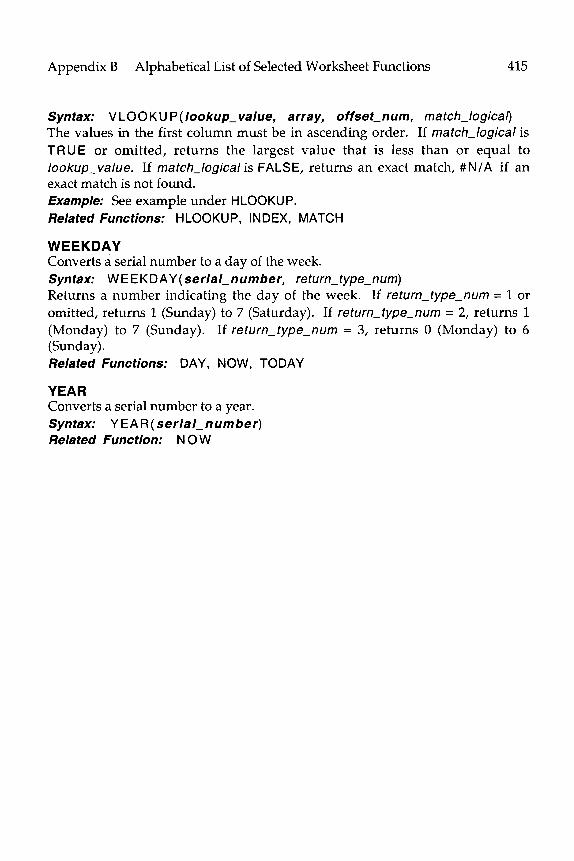
Appendix B Alphabetical List of Selected Worksheet Functions 415
Syntax: VLOOKU P(lookup value, array, offset-num, match-logical’) The values in the first columnmust be in ascending order. If matchJogica/ is TR U E or omitted, returns the largest value that is less than or equal to lookup - value. If match logical is FALSE, returns an exact match, #N/A if an - exact match is not found. Example; See example under HLOOKUP. Related Functions: HLOOKUP, INDEX, MATCH
WEEKDAY Converts a serial number to a day of the week. Syntax: WEEKDAY(serial number, return type num) Returns a number indicating the day of the week. -If return type-num = 1 or - omitted, returns 1 (Sunday) to 7 (Saturday). If return-type-num = 2, returns 1 (Monday) to 7 (Sunday). If return-type-num = 3, returns 0 (Monday) to 6 (Sunday) l
Related Functions: DAY, NOW, TODAY
YEAR Converts a serial number to a year. Syntax: YEAR(serial-number) Related Function: N 0 W

C SELECTED
VISUAL BASIC KEYWORDS BY CATEGORY
This appendix lists selected VBA keywords (reserved words) for functions, statements, methods and Pronerties. See Excel’s On-line Help for a complete list of keywords.
FUNCTIONS Abs Array Asc Atn Chr cos
EXP Fix Format InputBox Int IsArray IsDate IsEmpty IsMissing
IsNull
IsNumeric
LBound LTrim LCase Left
Returns the absolute value of a number. Returns a Variant containing an array. Returns the numeric code for the first character of text. Returns the angle corresponding to a tangent value. Returns the character corresponding to a code. Returns the cosine of an angle. Returns e raised to a power. Truncates a number to an integer. Formats a value according to a formatting code expression. Displays an input dialog box and waits for user input. Rounds a number to an integer. Returns True if the variable is an array. Returns True if the expression can be converted to a date. Returns True if the variable has been initialized. Returns True if an optional argument has not been passed to a procedure. Returns True if the expression is null (i.e., contains no valid data). Returns True if the expression can be evaluated to a number. Returns the lower limit of an array dimension. Returns a string without leading spaces. Converts a string into lowercase letters. Returns the leftmost characters of a string.
417
Excel for Chemists: A Comprehensive Guide. E. Joseph BilloCopyright 2001 by John Wiley & Sons, Inc.
ISBNs: 0-471-39462-9 (Paperback); 0-471-22058-2 (Electronic)

418 Excel for Chemists
Len
Log Mid
Returns the length (number of characters) in a string. Returns the natural (base-e) logarithm of a number. Returns a specified number of characters from a text string, beginning at a specified position.
MsgBox Displays a message box. Now Returns the current date and time. Right Returns the rightmost characters of a string. Rnd Returns a random number between 0 and 1. RTrim Returns a string without trailing spaces.
SW Returns the sign of a number. Sin Returns the sine of an angle.
SW Returns the square root of a number. Str Converts a number to a string. Tan Returns the tangent of an angle. Trim Returns a string without leading or trailing spaces. UBound Returns the upper limit of an array dimension. UCase Converts a string into uppercase letters. Val Converts a string to a number.
STATEMENTS (COMMANDSS) Beep Makes a “beep” sound. Call Dim Do...Loop Else Elself End Exit For Each...Next For...Next Function GoSub GoTo If...Then...End If On...GoSub
Transfers control to a Function or Sub procedure. Declares an array and allocates storage for it. Delineates a block of statements to be repeated. Optional part of If-Then structure. Optional part of If...Then structure. Terminates a procedure or block. Exits a Do . . . . For . . . . Function... or Sub... structure. Delineates a block of statements to be repeated. Delineates a block of statements to be repeated. Marks the beginning of a Function procedure. Branches to a subroutine within a procedure. Unconditional branch within a procedure. Delineates a block of conditional statements. Branches to one of several specified subroutines, depending on the value of an expression. Branches to one of several specified lines, depending on the value of an expression. Used at module level to declare lower bound for an array. Preserves data in an existing array when using Re Di m . Indicates that the procedure is available to all other procedures.
On...GoTo
Option Base Preserve Private

ADnendix C AA
Selected Visual Basic Keywords by Category 419
Public Indicates that the procedure is available only to
ReDim Return Select Case
Set Static stop Sub Until While With...End With
procedures in the same module. Allocates or re-allocates dynamic array storage. Delineates the end of a subroutine within a procedure. Executes one of several blocks of statements, depending on the value of an expression. Assigns an object reference to a variable. Preserves a procedures local variables between calls. Stops execution, but does not close files or clear variables. Marks the beginning of a Sub procedure. Optional part of Do...Loop structure Optional part of Do...Loop structure Delineates a block of statements to be executed on a single object.
METHODS Activate Address Cells Clear Close Columns
Activates an object.
COPY
Returns a reference, as text Returns a single cell by specifying the row and column. Clears formulas and formatting from a range of cells. Closes a window, workbook or workbooks. Returns a Range object that represents a single column or multiple columns. Copies the selected object to the Clipboard or to another location.
cut Cuts the selected object to the Clipboard or to another location.
Delete FillDown
FillRight
InputBox Insert MacroOptions Paste Quit Range
Rows
Deletes the selected object. Copies the contents and format(s) of the top cell(s) of a specified range into the remaining rows. Copies the contents and format(s) of the leftmost cell(s) of a specified range into the remaining columns. Displays an input dialog box and waits for user input. Inserts a range of cells in a worksheet. Sets options in the Macro Options dialog box. Pastes the contents of the Clipboard onto a worksheet. Quits Microsoft Excel. Returns a Range object that represents a cell or range of cells. Returns a Range object that represents a single row or multiple rows.
Save Saves changes to active workbook.

420 Excel for Chemists
SaveAs
Select Sort
PROPERTIES ActiveCell ActiveSheet Bold Column
Count Font Formula FontStyle Italic Name NumberFormat Row
Selection Text Value
Saves changes to active workbook or other document with a different filename. Selects an object. Sorts a range of cells.
Returns the active cell of the active window. Returns the active sheet of the active workbook. Returns True if the font is Bold. Sets the Bold font. Returns a number corresponding to the first column in the range. Returns the number of items in the collection. Returns the font of the object. Returns or sets the formula associated with an object. Returns or sets the font of the object. Returns True if the font is Italic. Sets the Italic font. Returns or sets the name of an object. Returns or sets the number format code of a cell. Returns a number corresponding to the first row in the range. Returns the selected object. Returns or sets the text associated with an object. Returns the value of an object.
OTHER KEYWORDS AND OPERATORS False Boolean kevword. True And Or
Boolean keyword. Logical operator. Logical operator.

D ALPHABETICAL LIST
OF SELECTED VISUAL BASIC KEYWORDS
This listing of VBA functions, statements, methods and properties will be useful when creating your own macros. For each VBA keyword, the required syntax is given, along with some comments on the required and optional arguments, one or more examples and a list of related keywords. See Excel’s On- line Help for further information.
Abs Function Returns the absolute value of a number. Syntax: Abs(number) Example: Abs(-7.3) returns 7.3 See also: Sgn
Activate Method Activates an object. Syntax: object.Activate Object can be Chart, Worksheet or Window. Example: Workbooks(“BOOK1 .XLS”).Worksheets(“Sheetl”).Activate See also: Select
ActiveCell Property Returns the active cell of the active window. Read-only. Syntax: ActiveCell and Application.ActiveCell are equivalent. See also: Activate, Select
ActiveSheet Property Returns the active sheet of the active workbook. Read-only. Syntax: object+tiveSheet Object can be Application, Window or Workbook. Example: Application.ActiveSheet.Name returns the name of the active
421
Excel for Chemists: A Comprehensive Guide. E. Joseph BilloCopyright 2001 by John Wiley & Sons, Inc.
ISBNs: 0-471-39462-9 (Paperback); 0-471-22058-2 (Electronic)

422 Excel for Chemists
sheet of the active workbook. Returns None if no sheet is active. See also: Activate, Select
Address Method Returns a reference, as text Syntax: object.Address (rowAbsolute,columnAbsolute, referencestyle, external, relative To) All arguments are optional. If rowAbsolute or columnAbsolute are True or omitted, returns that part of the address as an absolute reference. ReferenceStyle can be xlA1 or xlRlC1. If externa/ is True, returns an external reference. See On-line Help for information about the relativeTo argument. See a/so: Offset
Array Function Returns a Variant containing an array. Syntax: Array (arglist) Example: Array (31,28,37,30,37,30,31,37,30,37,30,3f) See also: Dim
Asc Function Returns the numeric code for the first character of text. Syntax: Asc(character) Example: Asc (“A”) returns 65. See also: Chr
Atn Function Returns the angle corresponding to a tangent value. Syntax: Atn(number) Number can be in the range - to +m. The returned angle is in radians, in the range --z/2 to +n;/2 (-90’ to 90’). To convert the result to degrees, multiply by 180/x Example: Atn(l) returns 0.785388573 or 45 degrees See also: Cos, Sin, Tan
Beep Command Makes a “beep” sound. Syntax: B e e p
Bold Property Returns True if the font is Bold. Sets the Bold font. Read-write. Syntax: object.Bol d Object must be Font. Example: Range(“A1 :El “).Font.Bold = True makes the cells bold. See also: Italic

Appendix D Alphabetical List of Visual Basic Keywords 423
Call Command Transfers control to a Function or Sub procedure. Syntax: Call name (argumentI, . ..) Name is the name of the procedure. ArgumentI, etc., are the names assigned to the arguments passed to the procedure. C a I I is optional; if omitted, the parentheses around the argument list must also be omitted. Example: Call Task1 (argument1 ,argument2) See also: Sub, Function
Cells Method Returns a single cell by specifying the row and column. Syntax: object.Cells(fow, column) Object is optional; if not specified, Cells refers to the active sheet. Example: Cells(2,1).Value = 5 enters the value 5 in cell A2. See a/so: Range
Chr Function Returns the character corresponding to a code. Syntax: Chr(number) Number must be between 1 and 255. Example: Chr(65) returns A. See also: Asc
Clear Method Clears formulas and formatting from a range of cells. Syntax: object.Clear Object can be Range (or ChartArea). Example: Range(“A1 :Cl O”).Clear See a/so: ClearContents, ClearFormats in Excel’s On-line Help.
Close Method Closes a window, workbook or workbooks. Syntax: For workbooks, use object,Close. For a workbook or window, use object.CIose(SaveChangesLogical, FileName). Object can be Window, Workbook or Workbooks. If SaveChangesLogicalis False, does not save changes; if omitted, displays a “Save Changes?” dialog box. Example: Workbooks(“BOOK1 .XLS”).Close See a/so: Open, Save, SaveAs
Column Property Returns a number corresponding to the first column in the range. Read-only. Syntax: 0bject.C 0 I u m n Object must be Range. See also: Columns, Row, Rows

424 Excel for Chemists
Columns Method Returns a Range object that represents a single column or multiple columns Syntax: object.CoIumns(index) Object can be Worksheet or Range. lndexis the name or number (column A = 1, etc.) of the column. Example: Selection.Columns.Count returns the number of columns in the selection. See also: Range, Rows
ColumnWidth Property Returns or sets the width of all columns in the range. If columns in the range have different widths, returns N u I I. Example: Worksheets(“Sheet1 “).Columns(“C”).ColumnWidth = 30 See also: RowHeight
Copy Method Copies the selected object to the Clipboard or to another location. Syntax: object.Copy(destination) Object can be Range, Worksheet, Chart and many other objects. Destination specifies the range where the copy will be pasted. If omitted, copy goes to the Clipboard. Example: Worksheets(“Sheet1 “).Range(“Al :CSO”).Copy See a/so: Cut, Paste
Cos Function Returns the cosine of an angle. Syntax: Cos(number) Number is the angle in radians; it can be in the range --oo to +m. To convert an angle in degrees to one in radians, multiply by n/180. Returns a value between -1 and 1. See also: Atn, Sin, Tan
Count Property Returns the number of items in the collection. Read-only. Syntax: object.Count Object can be any collection. Example: The statement N = array.Count counts the number of values in the range array.
Cut Method Cuts the selected object to the Clipboard or to another location. Syntax: object.Cut(destination) Object can be Range, Worksheet, Chart or one of many other objects. Destination specifies the range where the copy will be pasted. If omitted, copy

Appendix D Alphabetical List of Visual Basic Keywords 425
goes to the Clipboard. Example: Worksheets(“Sheet1 “).Range(“Al :C50”).Cut See also: Copy, Paste
CVErr Function Returns a Variant containing an error value specified by the user. Syntax: CVErr(number) CVErr can return either Excel’s built-in worksheet error values, or a user- defined error value. The values of number for built-m worksheet error values are xlErrDiv0, xlErrNA, xlErrName, xlErrNull, xlErrNum, xlErrRef, xlErrValue. See also: IsError
Delete Method Deletes the selected object. Syntax: object.DeIete(shift) Object can be Range, Worksheet, Chart and many other objects. Shift specifies how to shift cells when a range is deleted from a worksheet (xlToLeft or XIU p). Can also use shift = 1 or 2, respectively. If shift is omitted, Excel moves the cells without displaying the Shift Cells? dialog box. Example: Worksheets(“Sheetl2”).Range(“Al :A1 O”).Delete (xlToLeft) deletes the indicated range and shifts cells to left.
Dim Command Declares an array and allocates storage for it. Syntax: Dim variable (subscripts) Variable is the name assigned to the array. Subscripts are the dimensions of the array; an array can have up to 60 dimensions. Each dimension has a default lower value of zero; a single number for a dimension is taken as the upper limit. Use lower To upper to specify a range that does not begin at zero. Use Dim with empty parentheses to specify an array whose dimensions are defined within a procedure by means of the ReDim statement. Example: Dim Matrix ($5) creates a 6 x 6 array. See a/so.= ReDim
Do...Loop Command Delineates a block of statements to be repeated. Syntax: The beginning of the loop is delineated by Do or Do Until condition or Do While condition. The end of the loop is delineated by Loop or Loop Until condition or Loop While condition. Condition must evaluate to True or False. Example: See examples of Do...Loop structures in Chapter 14. See also: Exit, For, Next, Wend, While

426
Else Command Optional part of If...Then structure.
Excel for Chemists
Elself Command Optional part of If...Then structure.
End Command Terminates a procedure or block. Syntax: End terminates a procedure. End Function is required to terminate a Function procedure. End If is required to terminate a block If structure. End Select is required to terminate a Select Case structure. End Sub is required to terminate a Sub procedure. End With is required to terminate a With structure. Example: See examples under Select Case. See also: Exit, Function, If, Then, Else, Select Case, Sub, With
Exit Command Exits a Do . . . . For . . . . Function... or Sub... structure. Syntax: Exit Do, Exit For, Exit Function, Exit Sub From a Do or For loop, control is transferred to the statement following the Loop or Next statement, or, in the case of nested loops, to the loop that is one level above the loop containing the Exit statement. From a Function or Sub procedure, control is transferred to the statement following the one that called the procedure. Example: See examples of Exit procedures in Chapter 14. See a/so: Do, For...Next, Function, Stop, Sub
Exp Function Returns e raised to a power. Syntax: Exp(number) Returns the value of e raised to the power number. See a/so: Log
False Keyword Use the keywords True or False to assign the value True or False to Boolean (logical) variables. When other numeric data types are converted to Boolean values, 0 becomes False while all other values become True. When Boolean values are converted to other data types, False becomes 0 while True becomes -1. Example: If SubFlag = False Then... See also: True

Appendix D Alphabetical List of Visual Basic Keywords 427
FillDown Method Copies the contents and format(s) of the top cell(s) of a specified range into the remaining rows. Syntax: object.FillDown Object must be Range. Example: Worksheets(“Sheetl2”).Range(“Al :A1 O”).FillDown See also: FillLeft, FillRight, FillUp in Excel’s On-line Help.
FillRight Method Copies the contents and format(s) of the leftmost cell(s) of a specified range into the remaining columns. Syntax: object.FillDown Object must be Range. Example: Worksheets(“Sheetl2”).Range(“Al :A1 O”).FillRight See also: FillDown, FillLeft, FillUp in Excel’s On-line Help.
Fix Function Truncates a number to an integer. Syntax: Fix(number) If number is negative, Fix returns the first negative integer greater than or equal to number. Example: Fix(-2.5) returns -2. See also: Int
Font Property Returns the font of the object. Read-only. Syntax: object.Fo n t Example: ActiveCell.Font.Bold = True makes the characters in the active cell bold. See a/so: FontStyle
FontStyle Property Returns or sets the font of the object. Read-write. Syntax: object.FontStyle Example: Range(“A1 :El”).Font.FontStyle = “Bold” See also: Font
For...Next Command Delineates a block of statements to be repeated. Syntax: For counter = start To end Step increment
(statements) Next counter
Step increment is optional; if not included, the default value 1 is used. hcrement can be negative, in which case start should be greater than end.

428 Excel for Chemists
Example: See examples of For...Next procedures in Chapter 14. See also: Do...Loop, Exit, For Each...Next, While...Wend
For Each...Next Command Delineates a block of statements to be repeated. Syntax: For Each element In group
(statements) Next element
Group must be a collection or array. Element is the name assigned to the variable used to step through the collection or array. Group must be a collection or array. Example: See examples of For Each...Next procedures in Chapter 14. See also: Do...Loop, Exit, For...Next, While...Wend
Format Function Formats a value according to a formatting code expression. Syntax; Format(expression,formattext) Expression is usually a number, although strings can also be formatted. Formattext is a built-in or custom format. Additional information can be found in Microsoft Excel/Visual Basic Reference, or VBA On-line Help. Example: Format(TelNumber,“(###) ###-####“) formats the value TelNumber in the form of a telephone number.
Formula Property Returns or sets the formula in a cell. If a cell contains a value, returns the value; if the cell contains the formula, returns the formula as a string. See also; Text, Value
Function Command Marks the beginning of a Function procedure. Syntax: Function name argumentl, . . . Name is the name of the variable whose value is passed back to the caller. Argumentl, etc., are the names assigned to the arguments passed from the caller to the procedure. Example: See examples of Function procedures in Chapter 14. See also: Call, Sub
GoSub Command Branches to a subroutine within a procedure. Syntax: GoSub label The beginning of the subroutine is delineated by label, which can be a name or a line number. The end of the subroutine is delineated by one or more Return statements. The subroutine must be within the calling procedure. Example: See examples of subroutines in Chapter 14.

Appendix D Alphabetical List of Visual Basic Keywords 429
See also; GoTo, On...GoSub, On...GoTo, Return, Sub
GoTo Command Unconditional branch within a procedure. Syntax: GoTo label Label can be a name or a line number. See also: GoSub
If...Then...Else...End If Command Delineates a block of conditional statements. Syntax: If condition Then . . . Else . . . End If The statement can be all on one line (e.g., If condition Then statement). Alternatively, a block If structure can be used, in which case the first line consists of If condition Then; the end of the structure is delineated by End If. Condition must evaluate to True or False. The ellipsis following Then and Else can represent a single statement or several statements separated by colons; these are executed if concWon is True or False, respectively. Examples: If Char = ‘7 Then GoTo 2000
If (Char >= “0” And Char <= “9”) Then (statements) End If
See also; Elself, End
InputBox Function Displays an input dialog box and waits for user input. Syntax: InputBox(prompt,title,default,xpos,ypos,helpfile,context) See Microsoft ExceZ/Visual Basic Reference or On-line Help for details. See also; InputBox Method, MsgBox
InputBox Method Displays an input dialog box and waits for user input. Syntax: object.lnputBox(prompt,tit/e,defau/t,/eft,top,helpfi/e,context,
type) Objet t must be Ap pl i cat i on. See Microsoft Excel/Visual Basic Reference or On- line Help for details. See a/so: InputBox Function, MsgBox
Insert Method Inserts a range of cells in a worksheet. Syntax: object.lnsert(shift) Object is a Range object. Shift specifies how to shift cells when a range is inserted in a worksheet (xlToRight or xlDown). Can also use shift = 1 or 2, respectively. If shift is omitted, the Shift Cells? dialog box is not displayed. Examples: Worksheets(“Sheetl2”).Range(“Al :A1 O”).lnsert (1) inserts

430 Excel for Chemists
the indicated range and shifts cells to right. Worksheets(“Sheet1 “).Columns(4).Insert inserts a new column to the left of column D. See a/so: Delete
Int Function Rounds a number to an integer. Syntax: Int(number) If number is negative, Int returns the first negative integer less than or equal to number. Example: lnt(-2.5) returns -3. See a/so: Fix
IsArray Function Returns True if the variable is an array. Syntax: IsArray(name) See also: other Is functions
IsDate Function Returns True if the expression can be converted to a date. Syntax: IsDate( expression) See also: other Is functions
IsEmpty Function Returns True if the variable has been initialized. Syntax: IsEmpty(expression) See a/so: other Is functions
IsMissing Function Returns True if an optional argument has not been passed to a procedure. Syntax: IsMissing(name) See also: other Is functions
IsNull Function Returns True if the expression is null (i.e., contains no valid data). Syntax: IsNuII(expression) See also: other Is functions
IsNumeric Function Returns True if the expression can be evaluated to a number. Syntax: IsNumeric(expression) See also: other Is functions

Appendix D Alphabetical List of Visual Basic Keywords 431
Italic Property Returns True if the font is Italic. Sets the Italic font. Read-write. Syntax: object.ltalic Object must be Font. Example: Range(“A1 :El “).Font.ltalic = True makes the cells italic. See also: Bold
LBound Function Returns the lower limit of an array dimension. Syntax: LBound(array,dimension) Array is the name of the array. Dimension is an integer (1, 2, 3, etc.) specifying the dimension to be returned; if omitted, the value 1 is used. Example: If the array table was dimensioned using the statement Di m table (1 To 3, lOOO), LBound(table,l) returns 1, LBound(table,2) returns 0. See a/so: Dim, UBound
LCase Function Converts a string into lowercase letters. Syntax: L C a s e (s king) See also: UCase
LTrim Function Returns a string without leading spaces. Syntax: LTrim(string) See a/so: RTrim
Left Function Returns the leftmost characters of a string. Syntax: Left(string,number) If number is zero, a null string is returned. If number is greater than the number of characters in string, the entire string is returned. Example: Left(“CHEMISTRY”,4) returns CHEM See also: Len, Mid, Right
Len Function Returns the length (number of characters) in a string. Syntax: Len(string) Example: Len(“CHEMISTRY”) returns 9. See also; Left, Mid, Right
Log Function Returns the natural (base-e) logarithm of a number. Syntax: Log(number) Number must be a value or expression greater than zero. VBA does not provide base-10 logarithms; use Log(value)/Log(lO).

432 Excel for Chemists
See also: Exp
MacroOptions Method Sets options in the Macro Options dialog box. Synfax: AppIication.MacroOptions(macro, description, hasMenu, menuText, hasShortcutKey, shortcutKey, category, statusbar, helpcontext, helpfile)
macro is the name of the macro. description is the description that appears in the dialog box. category is the function category that the macro appears in: Financial, 1; Date & Time, 2; Math & Trig, 3; Statistical, 4; Lookup & Reference, 5; Database, 6; Text, 7; Logical, 8; Information, 9; User Defined, 14; Engineering, 15. Example: Application.MacroOptions macro:=“FtoC”, Description:= “Converts Fahrenheit temperature to Celsius”, Category:=3 provides a description for the macro FtoC and assigns it to the Math & Trig category.
Mid Function Returns the specified number of characters from a text string, beginning at the specified position. Syntax: Mid(string,start,number) If start is greater than the number of characters in string, returns a null string. If number is omitted, all characters from start to the end of the string are returned. Example: Mid(“H2S04”,2,1) returns 2. See also: Left, Len, Right
MsgBox Function Displays a message box. Syntax: MsgBox(prompt,buttons,title,helpfile,context) See Microsoft Excel/Visual Basic Reference or On-line Help for details. See also: InputBox
Name Property Returns or sets the name of an object. Example: SeriesName = Selection.Name assigns the name of the selected chart series to the variable SeriesName. See also: NameLocal, Names
Now Function Returns the current date and time. Syntax: N o w See also: other date and time functions.
NumberFormat Property Returns or sets the number format code of a cell. Example: Range(“A1 :A1 O”).NumberFormat= “0.00” sets the number

Appendix D Alphabetical List of Visual Basic Keywords 433
format of the specified range of cells. See also: GoSub, GoTo, Return, Select Case
On...GoSub Command Branches to one of several specified subroutines, depending on the value of an expression. Syntax: On expression GoSub labell, . . . Control is transferred to the label (line number or label) determined by the value of expression. Expression is any expression that evaluates to a number; if not an integer, it is rounded to the nearest whole number. The number must be between 0 and 255. Example; See examples of On...GoSub procedures in Chapter 14. See a/so: GoSub, GoTo, Return, Select Case
On...GoTo Command Branches to one of several specified lines, depending on the value of an expression. Syntax: On expression GoTo labell, . . . See explanation under On...GoSub Command. Example: See examples of On...GoTo procedures in Chapter 14. See also: GoSub, GoTo, Return, Select Case
Open Method Opens a workbook. Syntax: object.Open(fi/ename, . ..) Object must be Workbooks. Filename is required. See On-line Help for the remaining arguments: Example: Workbooks.Open(“SOLVSTAT.XLS”) See a/so: Close, Save, SaveAs
Option Base Statement Used at module level to declare lower bound for an array. Can be Option Base 0 or 1. The statement can appear only once in a module and must precede all Dim or equivalent declaration. See a/so: Dim, LBound, ReDim
Paste Method Pastes the contents of the Clipboard onto a worksheet. Syntax: object.Paste(destination) Object must be Worksheet. There are other Paste methods, with different syntax, for Chart and many other objects. Destination specifies the range where the copy will be pasted. If omitted, copy is pasted to the current selection. Example: Worksheets(“Sheet1 “).Range(“Al :C5O”).Copy
ActiveSheet.Paste See also: Copy, Cut

434 Excel for Chemists
ParamArray Command Allows the use of an indefinite number of arguments for a function. The specified argument is an Optional array of Variant elements. See a/so: Dim, Function
Preserve Command Preserves data in an existing array when using ReDim.
Private Command Indicates that the procedure is available to all other procedures.
Public Command Indicates that the procedure is available only to procedures in the same module.
Quit Method Quits Microsoft Excel. Syntax: 0bject.Q u it Object must be Application. Example: Application.Quit See also: Close, Save
Range Method Returns a Range object that represents a cell or range of cells. Syntax: object.Range(reference) Object is required if it is Worksheet. Reference must be an Al-style reference, in quotes, or the name of the reference. Example: Worksheets(“Sheetl2”).Range(“Al”).Value = 5 See also: Cells
ReDim Command Allocates or re-allocates dynamic array storage. Syntax: ReDim variab/e (subscripts) For discussion of variable and subscripts, see comments under the entry for Dim. You can use ReDim repeatedly to change the number of elements in an array, or the number or dimensions. Example: Di m Matrix0
(statements) ReDim Matrix (5,5) (statements) ReDim Matrix (15,25)
See also: Dim
Return Command Delineates the end of a subroutine within a procedure. See also: GoSub

Appendix D Alphabetical List of Visual Basic Keywords 435
Right Function Returns the rightmost characters of a string. Syntax: Right(string,number) If number is zero, a null string is returned. If number is greater than the number of characters in string, the entire string is returned. Example= Right(303585842,4) returns 5842. See also: Left, Len, Mid
Rnd Function Returns a random number between 0 and 1. Syntax: R n d
Row Property Returns a number corresponding to the first row in the range. Read-only. Syntax: 0bject.R o w Object must be Range. Example: If ActiveCelLRow = IO Then ActiveCell.Interior.Colorlndex = 27 changes the interior color of the active cell to yellow if it is in row 10. See also: Column, Columns, Rows
RowHeight Property Returns or sets the height of all rows in the range. Example: Worksheets(“Sheetl”).Rows(l).RowHeight = 15 See also: ColumnWidth
Rows Method Returns a Range object that represents a single row or multiple rows. Syntax: object.Rows(index) Object can be Worksheet or Range. Indexis the name or number of the row. Example: Selection.Rows.Count returns the number of rows in the selection. See a/so: Columns, Range
RTrim Function Returns a string without trailing spaces. Syntax: RTrim(string) See also: LTrim, Trim
Save Method Saves changes to active workbook. Syntax: object.Save( filename) Object must be Workbook. If filename is omitted, uses a default name. Example: ActiveWorkbook.Save See also: Close, Open, SaveAs

436 Excel for Chemists
SaveAs Method Saves changes to active workbook or other document with a different filename. Syntax: object.SaveAs(fi/ename, . ..) Object can be Worksheet, Workbook, Chart or other document types. See Microsoft Excel/Visual Basic Reference or On-line Help for details. Example: NewChart.SaveAs(“New Chart”) See also: Close, Open, Save
Select Method Selects an object. Syntax: objectSelect Object can be Chart, Worksheet or one of many other objects. Example: Range(“A1 :C5O”).Select See also: Activate
Select Case Command Executes one of several blocks of statements, depending on the value of an expression. Syntax: Select Case expression
Case expression I (statements) Case expression2 (statements) End Select
You can also use the To keyword in expression , e.g., Case “A” To “M”. Expression can also be a logical expression. Use Case Else (not required) to handle all cases not covered by the preceding Case statements. Example: See examples of Select Case procedures in Chapter 14. See also: If...Then...Else, On...GoSub, On...GoTo
Selection Property Returns the selected object. The object returned depends on the type of selection. See also: Activate, ActiveCell, Select
Set Command Assigns an object reference to a variable. See a/so: Dim, ReDim
Sgn Function Returns the sign of a number. Syntax: Sgn(number) Returns 1, 0 or -1 if number is positive, zero or negative, respectively. Example: Sgn(-7.3) returns -1. See also: Abs’

Appendix D Alphabetical List of Visual Basic Keywords 437
Sin Function Returns the sine of an angle. Syntax: Sin(number) Number is the angle in radians; it can be in the range --oo to +=. To convert an angle in degrees to one in radians, multiply by n/180. Returns a value between -1 and 1. See also: Atn, Cos, Tan
Sort Method Sorts a range of cells. Syntax: objectSort(sortkeyl,orderI,sortkey2,order2, . ..) Object must be Range. See Microsoft Excel/Visual Basic Reference or On-line Help for details.
Sqr Function Returns the square root of a number. Syntax: Sqr(number) Number must be greater than or equal to zero.
Stop Command Stops execution, but does not close files or clear variables. See a/so: End
Str Function Converts a number to a string. Syntax: Str(number) A leading space is reserved for the sign of the number; if the number is positive, the string will contain a leading space. See also: Format
Sub Command Marks the beginning of a Sub procedure. .
Syntax: Sub name argumentl, . . . Name is the name of the procedure. ArgumentI, etc., are the names assigned to the arguments passed from the caller to the procedure. The end of the procedure is delineated by End Sub Example: See examples of Sub procedures in Chapter 14. See also: Call, Function
Tan Function Returns the tangent of an angle. Syntax: Tan(number) Number is the angle in radians; it can be in the range --oo to +=. To convert an angle in degrees to one in radians, multiply by n/180. Returns a value between - and +m.

438 Excel for Chemists
See also: Atn, Cos, Sin
Text Property Returns or sets the text associated with an object. The text can be associated with a chart, button, textbox, control or range. For all except range, this property is read-write, but for a range, it is read-only. Example: Worksheets(“Sheetl”).Buttons(l).Text = “Undo” See a/so: Formula, Value
Trim Function Returns a string without leading or trailing spaces. Syntax: T r i m (string) See also: LTrim, RTrim
True Keyword Use the keywords True or False to assign the value True or False to Boolean (logical) variables. When other numeric data types are converted to Boolean values, 0 becomes False while all other values become True. When Boolean values are converted to other data types, False becomes 0 while True becomes -1. Example: If FirstFlag = True Then GoTo 2000 See also: False
UBound Function Returns the upper limit of an array dimension. Syntax: U B o u n d (array, dimension) Array is the name of the array. Dimension is an integer (1, 2, 3, etc.) specifying the dimension to be returned; if omitted, the value 1 is used. Example: If the array table was dimensioned using the statement Dim table (1 To 3, lOOO), UBound(table,3) returns 1, UBound(table,2) returns 1000. See also: Dim, LBound
UCase Function Converts a string into upper case letters. Syntax: UCase(string) See also: LCase
Until Command Optional part of Do...Loop structure. Syntax: See explanation under Do...Loop.
Val Function Converts a string to a number. Syntax: Val(stl;ing) Val stops at the first non-numeric character other than the period.

Appendix D Alphabetical List of Visual Basic Keywords
Example: Val(“21 Lawrence Avenue”) returns 21. See also: Str
Value Property Returns the value of an object. Syntax: object.Value If object is Range, returns or sets the value(s) of the cell(s). Read-write. If Range contains more than one cell, returns an array of values. Example; Worksheets(“Sheetl2”).Range(“Al “).Value = “Volume, mL”
Wend Command Delineates the end of a While...Wend procedure. Syntax: See explanation under Do...Loop. See also: Do...Loop, While...Wend
While Command Executes a series of statements as long as a specified condition is true. Syntax: See explanation under Do...Loop. See also: Do...Loop, Wend With...End With Command Delineates a block of statements to be executed on a single object. Syntax: With object
(statements) End With
Example: With ActiveSheet.PageSetup .CenterHeader = “DRAFT VERSION” .CenterFooter = “” End With
See also: Do...Loop, While...Wend
439

E SHORTCUT KEYS
FOR PC AND MACINTOSH
Adies PC I I
Key to”
arrow keys W
arrow keys D
arrow keys
right/ left arrow keys
W
C
right/ left arrow keys
D
up/ down C arrow keys
up/ down D arrow keys
BACKSPACE F
COMMAND W
CONTROL
(Excel 97, Excel 2000)
Move one cell in direction of arrow
Move between options in a group of options
Move selected object(s)
Select the next/previous element within a group of chart elements
Move one character to the right or left in the entry in an edit box
Select the next/previous chart element
Move between options in a list box
Delete character to the left of the insertion point, or selected character(s)
WA
Make a non-adjacent selection
Macintosh (Excel 98, Excel 2001)
Move one cell in direction of arrow
Move between options in a group of options
Move selected object(s)
Select the next/previous element within a group of chart elements
Move one character to the right or left in the entry in an edit box
Select the next/previous chart element
Move between options in a list box
N/A
Make a non-adjacent selection
Display a shortcut menu
(W = Worksheet, F = Formula bar, C = Chart, D = Dialog box, V = Visual Basic editor)
441
Excel for Chemists: A Comprehensive Guide. E. Joseph BilloCopyright 2001 by John Wiley & Sons, Inc.
ISBNs: 0-471-39462-9 (Paperback); 0-471-22058-2 (Electronic)

442 Excel for Chemists
CONTROL
DELETE
DELETE
END
END
END
ENTER
ENTER/
RETURN
ESC
ESC
ESC
HOME
HOME
HOME
INS
OPTION
SHIFT
TAB
W
F
W
D
F
W
F, w
D
D
F
WV
D
F
W
W
W
W
D
When using AutoFill, copy a cell or range rather than create a series
Delete character to the right of the insertion point
Delete contents of selected cells
Move to the end of the entry in an edit box
Extend selection to last-used cell (lower-right corner)
Toggle END mode on/off
Enter data and move down one cell
Perform the action assigned to the default button (usually the OK button)
Cancel and close the dialog box or shortcut menu
Undo editing
Halt execution of a macro
Move to the beginning of the entry in an edit box
Move insertion point to beginning
Select cell in column A in same row as active cell
Toggle between Insert and Typeover modes
N/A
Select multiple objects on worksheet
Move to the next option
When using AutoFill, display the shortcut menu
Clear selected character(s) to the left of the insertion point
Move to the end of the entry in an edit box
N/A
WA Enter data and move down one cell
Perform the action assigned to the default button (usually the OK button)
Cancel and close the dialog box or shortcut menu
Undo editing
Halt execution of a macro
Move to the beginnin entry in an edit box
Move insertion point beginning
g of the
to
Select cell in column A in same row as active cell
WA
When using AutoFill, copy a cell or range rather than create a series
Select multiple objects on worksheet
Move to the next option
(W = Worksheet, F = Formula bar, C = Chart, D = Dialog box, V = Visual Basic editor)

Appendix E Shortcut Keys for PC and Macintosh 443
TAB D Move to the next input box Move to the next input box
Move right one cell, or move to next unlocked cell in a protected worksheet
TAB W Move right one cell, or move to next unlocked cell protected worksheet
ina
TAB W Move to the next toolbutton Move to the next toolbu (when toolbar is active) (when toolbar is active)
tton
(space) D Perform the action assigned to the active button, or select or clear the active check box
Perform the action assigned to the active button, or select or clear the active check box
CONTROL+(key)
arrow keys W
F
Jump to end of block of data in direction of arrow
Move to beginning of next element in formula, in direction of arrow
Move one word to the right or left in the entry in an edit box
Jump to end of block in direction of arrow
of data
right/ left arrow keys
Move to beginning of next element in formula, in direction of arrow
right/ left arrow keys
D Move one word to the right or left in the entry in an edit box
Display active cell
Halt macro execution
Clear from insertion point to end
Select bottom right cell
Enter the contents of the formula bar in the selected range (references are adjusted)
Select next sheet in workbook
Switch to next tab
Select previous sheet in workbook
BACKSPACE
BREAK
DELETE
W
V
F
W
W
N/A
N/A Clear end
from insertion point to
END
ENTER/
RETURN
WA Enter the contents of the formula bar in the selected range (references are adjusted)
PAGE DOWN W
D
W
D
Select next sheet in workbook
PAGE DOWN
PAGE UP
Switch to next tab
Select previous sheet in workbook
PAGE UP Switch to previous tab Switch to previous tab
(W = Worksheet, F = Formula bar, C = Chart, D = Dialog box, V = Visual Basic editor)

444 Excel for Chemists
TAB
‘(apostrophe)
(space)
(space)
(space)
* (numeric
keypad)
-(minus)
. (period)
/(slash)
:(colon)
(semicolon) /
I
I
- (tilde)
w
W
V
V
W
W
W
W
W
W
W
W
W
W
W
W
W
Move to the previous toolbutton (when toolbar is active)
Copy value or formula from cell above (references are not adjusted)
Display global list of Methods and Properties (with cursor on blank line)
Jump to end of next element in line of code
Select entire column
Select block of data containing the active cell
Display the Delete.. . dialog box
Display the Delete.. . dialog box
Move clockwise to the next comer of the selection
Select all cells of the array containing the active cell
Insert current time
Insert current date
Move clockwise to the next comer of the selection
Select all cells of the array containing the active cell
Insert current time
Insert current date
Select cells that are direct Select cells that are direct precedents of cells in precedents of cells in selection selection
Select cells that are direct Select cells that are direct dependents of cells in dependents of cells in selection selection
values and Toggle between values and Toggle between formulas formulas
Hide column(s) containing Hide column(s) containing selection selection
Display the Format Cells dialog box
Apply or remove Bold formatting
Move to the previous toolbutton active)
(when toolbar is
Copy value or formula from cell above (references are not adjusted)
Select entire column
(W = Worksheet, F = Formula bar, C = Chart, D = Dialog box, V = Visual Basic editor)

Appendix E A A
Shortcut Kevs for PC and Macintosh J
A W Select entire worksheet
B W/F Apply or remove Bold Apply or remove Bold formatting formatting
C W/F COPY COPY D W Fill Down Fill Down
F W Display the Find... dialog box Display the Find... dialog box
G V Display Immediate window
G W Display the Go To... dialog Display the Go To... dialog box box
H W Display the Replace... dialog Display the Replace... dialog box box
I W/F Apply or remove Italic Apply or remove Italic formatting formatting
(W = Worksheet, F = Formula bar, C = Chart, D = Dialog box, V = Visual Basic editor)
W Apply or remove Italic formatting
W Apply or remove Underline formatting
W Apply or remove Strikethrough formatting
W Toggle between displaying Toggle between displaying objects, placeholders for objects, placeholders for objects or hiding objects objects or hiding objects
W Toggle display of Standard Toggle display of Standard toolbar toolbar
W Toggle display of outline Toggle display of outline symbols symbols
W Hide row(s) containing Hide row(s) containing selection selection
F Display the Formula Palette (the Insert Function Step 2 dialog box) after typing a function name in a formula
Display the Formula Palette (the Insert Function Step 2 dialog box) after typing a function name in a formula
445

446 Excel for Chemists
J
J
K
N
0
P
R
R
S
U
V
X
Y
Y
z
V
V
W
W
W
W
V
W
W
W
W/F
W/F
V
W
W
Display global list of Methods and Properties (with cursor on blank line)
Display list of Methods and Properties for selected object
Display the Insert Hyperlink dialog box
New (Open a new workbook)
Display the Open... dialog box
Display the Print... dialog box
Display the Project Explorer window
Display the Insert Hyperlink dialog box
New (Open a new workbook)
Display the Open... dialog box
Display the Print... dialog box
Fill Right
Save the active workbook
Apply or remove Underline formatting
Paste
cut
Delete line in a macro
Repeat
Undo
Fill Right
Save the active workbook
Apply or remove Underline formatting
Paste
cut
Repeat
Undo
SHIFT+(key )
arrow keys W
arrow keys W
right/ left arrow keys
D
Extend selection by one row/column
With END mode on, extend selection to end of block in direction of arrow
Select or unselect one char- acter to the right or left in the entry in an edit box
Extend selection by one row/column
WA
(W = Worksheet, F = Formula bar, C = Chart, D = Dialog box, V = Visual Basic editor)

Appendix E Shortcut Kevs for PC and Macintosh 447 A I
(space)
END
END
END
ENTER
HOME
HOME
HOME
HOME
RETURN
TAB
TAB
Select entire row W
D
F
W
W
D
F
W
W
W
D
W
Select entire row
N/A Select from the insertion point to the end of the entry in an edit box
Extend selection from insertion point to end of current line in formula
WA
Extend row
selection to end of N/A
Enter data and move up one Enter data and move up one cell cell
Select from the insertion point to the beginning of the entry in an edit box
Extend selection from insertion point to beginning of current line in formula
Extend selection from insertion point to beginning of current line in formula
Extend selection to beginning of row
Extend selection to beginning of row
N/A With END mode on, extend selection to last-used cell (lower-right comer)
With END mode on, extend selection to last cell in row
N/A
Move to the previous option
Enter data and move left one cell
Move to the previous option
Enter data and move left one cell
CONTROL+SHIFT+(key)
arrow keys F Select to end of block of data in direction of arrow (inserts
Select to end of block of data in direct ion of a rrow (inserts reference in formula) reference in formula)
arrow keys W Select to end of block of data in direction of arrow
Select to end of block of data in direction of arrow
right/ left arrow keys
F Extend selection, one term at Extend selection, one term at a time a time
(W = Worksheet, F = Formula bar, C = Chart, D = Dialog box, V = Visual Basic editor)

448 Excel for Chemists
right/ left arrow keys
END
END
ENTER/
RETURN
HOME
HOME
D
F
W
W
F
W
PAGE DOWN W
PAGE UP W
TAB D
! W
# W
$ W
0 / 0 W
& W
Select or unselect one word to the right or left in the entry in an edit box
Extend selection from insertion point to end of formula
Extend selection to end of worksheet (bottom right corner)
Enter an array formula in the selected range
Extend selection from insertion point to beginning of formula
Extend selection to beginning of worksheet (upper left comer)
Select current and next sheet in workbook
Select current and previous sheet in workbook
Switch to previous tab
Apply Decimal number format (two decimal places, thousands separator, minus sign for negative numbers)
Apply Date number format (d-mmm-yy)
Apply Currency number format (two decimal places, negative numbers in parentheses)
Apply Percent number format (no decimal places)
Apply Date number format (d-mmm-yy)
WA
N/A
Enter an array formula in the selected range
Extend selection from insertion point to of formula
beginning
Extend selection to beginning of worksheet (upper left corner)
Select curren in workbook
t and next sheet
Select current and previous sheet in workbook
Apply Decimal number format (two decimal places, thousands separator, minus sign for negative numbers)
Apply Date number
(d-m-=qy)
format
Apply Currency number format (two decimal places, negative numbers in parentheses)
Apply Percent number format (no decimal places)
Apply Date number format (d-mmm-yy)
(W = Worksheet, F = Formula bar, C = Chart, D = Dialog box, V = Visual Basic editor)

Appendix E Shortcut Kevs for PC and Macintosh 449 AA
(
>
* (asterisk)
+
@
A
- (tilde)
(space)
A
F
J 0
P
W
W
W
W
W
W
W
W
W
W
F
W
V
W
W
J
Unhide rows
Unhide columns
Select block of data containing the active cell
Display the Insert dialog box
Apply Time number format (hours and minutes, AM and PM)
Apply Scientific number format (two decimal places)
Select cells that are direct or indirect precedents of cells in selection
Select cells that are direct or indirect dependents of cells in selection
Apply General number format
Select entire worksheet
Insert placeholder arguments and closing parenthesis after typing a function name in a formula
Activate the Font list box
Display list of constants
Select all cells with comments
Activate the Font Size list box
Unhide rows
Unhide columns
Select block of data containing the active cell
Display the Insert dialog box
Apply Time number format (hours and minutes, AM and
PM)
APPlY Scien tific number format : (two decimal places)
Select cells that are direct or indirect precedents of cells in selection
Select cells that are direct or indirect dependents of cells in selection
Apply General number format
Select entire worksheet
Insert placeholder argument5 and closing parenthesis after typing a function name in a formula
Display the Format Cells dialog box
Display the Format Cells dialog box
(W = Worksheet,“F = Formula bar, C = Chart, D = Dialog box, V = Visual Basic editor)

450 Excel for Chemists
COMMAND+(key) [Macintosh only]
arrow keys W N/A
ENTER/
RETURN
-(hyphen)
. (period)
/
(semicolon) / -
W N/A
W
W
W
F
N/A
N/A
WA N/A
WA
W N/A
? W WA -(tilde) W N/A
1 W N/A
6 7 W
N/A N/A
8 W N/A
A W N/A B W N/A C W/F WA D W N/A
E, G J, M W WA F W N/A G V WA H W N/A
Jump to end of block of data in direction of arrow
Enter the contents of the formula bar in the selected range
Insert current date
Halt execution of a macro
Help
Insert current time
Calculate and display result of selection
Recalculate workbooks
all open
Display Help
Toggle between values and formulas
Display Format Cells dialog box
Find Next
Toggle display of Standard toolbar
Toggle display of outline symbols
Select entire worksheet
Clear Contents
COPY Fill Down
Not used
Display Find... dialog box
Display Immediate window
Display Replace... dialog bo>
(W = Worksheet, F = Formula bar, C = Chart, D = Dialog box, V = Visual Basic editor)

Appendix E
I
Is
L
N
0
I?
Q R
R
S
T
U
V
W
X
Y
Y
Z
Shortcut Keys for PC and Macintosh 451
W N/A Display Insert Cells... dialog box
W N/A Display Delete... Rows/Columns dialog box
W N/A Display Define Name dialog box
W N/A Insert New workbook
W N/A
W N/A
W N/A
V N/A
Display
Display
Quit
Display . 1
r
wmaow
W
W
F
W
W/F
W
W/F
V
W
W
N/A
N/A
N/A
N/A N/A
N/A N/A
N/A
WA WA
Open... dialog box
Print... dialog box
the Project Explorer
Fill Right
Save
Toggle between relative and absolute reference
Begin Edit mode
Paste
Close
cut
Delete line in a macro
Repeat
Undo
COMMAND+SHIFT+(key) [Macintosh only]
3 W N/A Create a picture file of the entire screen and save to hard drive as PictureN
4 W N/A Create a picture file of a selected region of the screen and save to hard drive as PictureN
(W = Worksheet; F = Formula bar, C = Chart, D = Dialog box, V = Visual Basic editor)

452 Excel for Chemists
A W N/A Move clockwise to the next corner of the selection
W,F N/A Apply or remove Bold formatting
Display Copy Picture dialog box.
B
C W N/A
W,F N/A Apply or remove Outline formatting
Find Next
D
G
I
W N/A
W,F N/A Apply or remove Italic formatting
J K L
N
0
W N/A
W N/A
W N/A
W N/A
W N/A
Ungroup
Group
Display the Style dialog box.
Insert a Cell Comment
Select all cells with comments
W,F N/A
W N/A
W N/A
Remove all formatting
Save
P
S
T Insert the SUM function in a cell
Apply or remove Underline formatting
U W,F N/A
W W,F N/A Apply or remove formatting
Shad
W N/A Select only visible cells in Z current selection
(W = Worksheet, F = Formula bar, C = Chart, D = Dialog box, V = Visual Basic editor)

ALT+(key) [PC only]
down arrow D
ENTER F
BACKSPACE W
‘(apostrophe) W
-(minus) W
(semicolon) W /
(letter) D
Open the selected drop-down N/A list box
Insert a line break N/A
Undo WA
Display the Style dialog box. N/A
Display the Workbook Icon N/A menu to Maximize/ Minimize/Restore a window
Select only visible cells in the N/A current selection
Select the menu or dialog box N/A option indicated by the underlined letter
Appendix E Shortcut Keys for PC and Macintosh r 45. L
COMMAND+OPTION+(key) [Macintosh only]
arrow keys W N/A
CONTROL+ALT+(key) [PC only]
right / left arrow keys
W Move between non-adjacent selections
Function Keys
Fl
F2
W Help
W Begin Edit. Position the insertion point at the end of the line.
F3
F4
W Display the Paste Name dialog box.
W Repeat
Apply border
N/A
Undo
cut
COPY
Paste
(W = Worksheet, F = Formula bar, C = Chart, D = Dialog box, V = Visual Basic editor)

454 Excel for Chemists
F4 F Toggle Absolute/Relative references
Display the Go To dialog box Display the Go To dialog
Move to the next pane in a split workbook
Display the Spell Check dialog box
Move to the next split workbook
pane ina
Display the Spell Check dialog box
Activate/deactivate Extend mode (then use arrow keys)
Recalculate all sheets in all open workbooks
Calculate and display result of selection
Activate/deactivate Extend mode (then use arrow keys)
Calculate and display of selection
Activate menu bar
Create a new chart that uses the current selection
Save the active workbook
Activate menu bar
Create a new chart tha the current selection
Save the active workbook
F5 W
F6 W
F7 W
F8 W
F9 W
F9 F
FlO
Fll
W
W
F12 W
SHIFT+(function key)
Help
Undo
Fl W Help
Fl V Get Help on a selected VBA keyword
Insert a Cell Comment F2 W Insert a Cell Comment
F2 V Display the Object Browser window
F3
F4
W Display the Paste Function dialog box
W Display the Find Next dialog box
Display the Paste Function dialog box
Display the Find Next dialog
F4 V Display the Properties window
F5 W Display the Find dialog box Display the Find dialog box
(W = Worksheet, F = Formula bar, C = Chart, D = Dialog box, V = Visual Basic editor)

Appendix E
F5
F6
F8
F8
F9
F9
FlO
Fll
F12
Shortcut Kevs for PC and Macintosh 455 J
Run a macro
Move to the previous pane in a workbook that has been split
Toggle Modify Selection mode
Step through macro
Recalculate the active worksheet
Toggle breakpoint
Display a shortcut menu
Insert a new worksheet
Display the Save As dialog box
V
W
W
V
W
V
W
W
W
Run a macro
Move to the previous pane ir a workbook that has been split
Toggle Modify Selection mode
Step through macro
Recalculate the active worksheet
Toggle breakpoint
Display a shortcut menu
Insert a new worksheet
Display the Save As dialog box
CONTROL+(function kev) J _
Display the Define Name dialog box
Close the active window
F3 W Display the Define Name dialog box
Close the active window
Restore window size
Move to the next workbook active window
Move the window (use arrow keys)
F4
F5
F6
W
W
W
Restore window size
Move to the next workbook active window
W Move
km
the window (use arrow F7
F8
F8
V
W
Run to cursor
Re-size the window (use arrow keys)
Re-size the window (use arrow keys)
Select statement to execute next
F9 V
Minimize the window
Maximize the window
Insert Excel 4 macro Sheet
Display Open dialog box
F9
FlO
Fll
F12
W
W
W
W
Toggle Window Maximize
Insert Excel 4 macro Sheet
Display Open dialog box
(W = Worksheet, F = Formula bar, C = Chart, D = Dialog box, V = Visual Basic editor)

456 Excel for Chemists
ALT+(function key) [PC only]
Fl
F2
F4
F6
F8
Fll
W Create a new chart that uses N/A the current selection
W Save the active workbook N/A
W Close N/A
W Switch to next window N/A
W Display Macro dialog box WA
W Toggle between Visual Basic N/A Editor and Excel
CONTROL+ALT+(function key) [PC only]
F9 W Recalculate all sheets in the N/A active workbook
OPTION+(function key) [Macintosh only]
F8 W N/A
FlO W N/A
Fll W N/A
CONTROL+SHIFT+(function key)
F3 W Display the Create Names dialog box
F4 W Display the Find Next dialog box
F6 W
F12 W Display Print... dialog box
Display Macro dialog box.
Make toolbar active (then USC arrow keys)
Toggle between Visual Basic Editor and Excel
Display the Create Names dialog box
Move to the previous workbook active window
Display Print... dialog box
ALT+SHIFT+(function key) [PC only]
Fl
F2
W Insert a New worksheet N/A
W Display the Save As dialog WA box
(W = Worksheet, F = Formula bar, C = Chart, D = Dialog box, V = Visual Basic editor)

F SELECTED SHORTCUT KEYS
FOR PC AND MACINTOSH, BY CATEGORY
PC (Excel 97, Excel 2000)
Cut, Copy, Paste, Undo
Undo CONTROL+Z or ALT+BACKSPACE
cut CONTROL+X
COPY CONTROL+C
Paste CONTROL+V
Clear contents of selection DELETE (formula bar or worksheet)
Repeat CONTROL+Y or F4
Moving and Selecting
Jump to end of block of data in direction of arrow
Select to end of block of data in direction of arrow (inserts reference in formula)
Select entire row
CONTROL+arrow key
CONTROL+SHIFT+ arrow key
SHIFT+(space)
Macintosh (Excel 98, Excel 2001)
CONTROL+Z or COMMAND+Z or Fl
CONTROL+X or COMMAND+X or F2
CONTROL+C or COMMAND+C or F3
CONTROL+V or COMMAND+V or F4
COMMAND+B
CONTROL+Y or COMMAND+Y
CONTROL+arrow key or COMMAND+arrow key
CONTROL+SHIFT+ arrow key
SHIFT+(space)
457
Excel for Chemists: A Comprehensive Guide. E. Joseph BilloCopyright 2001 by John Wiley & Sons, Inc.
ISBNs: 0-471-39462-9 (Paperback); 0-471-22058-2 (Electronic)

458 Excel for Chemists
Select entire column CONTROL+(space)
CONTROL+/ (slash)
CONTROL+(space)
CONTROL+/ (slash) Select all cells of the array containing the active cell
Extend selection by one SHIFT+arrow key SHIFT+arrow key row /column
CONTROL+SHIFT+right or left arrow key
CONTROL+0
Extend selection in a CONTROL+SHIFT+right or left arrow kev formula, one term at a time
Hide column(s) containing selection
CONTROL+0
Hide row(s) containing CONTROL+9 CONTROL+9 selection
Unhide rows CONTROL+SHIFT+(
CONTROL+SHIFT+)
CONTROL+SHIFT+” (asterisk) or CONTROL+* (numeric keypad)
ALT+;(semicolon)
CONTROL+SHIFT+(
CONTROL+SHIFT+)
CONTROL+SHIFT+” (asterisk)
Unhide columns
Select block of data containing the activ .e cell
Select only visible cells in the current selection
Select all cells with comments
COMMAND+SHIFT+Z
COMMAND+SHIFT+O
Select entire worksheet CONTROL+A
CONTROL+ALT+ right or left arrow key
Move between non- adjacent selections
CONTROL+OPTION+ right or left arrow key
Entering or Editing a Formula
Begin Edit. Position the F2 insertion point at the end of the line.
Enter the contents of the CONTROL+ENTER formula bar in the selected range (references are adjusted)
Insert current time CONTROL+:(colon)
CONTROL+ RETURN or COMMAND+ RETURN
CONTROL+:(colon) or COMMAND+;(semicolon)

Appendix F A A
Selected Shortcut Keys by Category 459
Insert current date
Insert a line break
Toggle between values and formulas
Display the Formula Palette (the Insert Function Step 2 dialog box) after typing a function name in a formula
Insert placeholder arguments and closing parenthesis after typing a function name in a formula
Enter data and move down one cell
Enter data and move up one cell
Enter data and move right one cell
Enter data and move left one cell
Enter an array formula in the selected range
Toggle between relative and absolute reference
Calculate and display result of selection
Fill Down
Fill Right
Formatting
Apply or remove Bold formatting
CONTROL+;(semicolon)
ALT+ENTER
CONTROL+- (tilde)
CONTROL+A
CONTROL+SHIFT+A
ENTER
SHIFT+ENTER
TAB
SHIFT+TAB
CONTROL+SHIFT+ ENTER
F4
F9
CONTROL+D
CONTROL+R
CONTROL+B
CONTROL+;(semicofon) or COMMAND+-
(hyphen)
COMMAND+OPTION+ RETURN
CONTROL+- or COMMAND+- (tilde)
CONTROL+A
CONTROL+SHIFT+A
RETURN
SHIFT+ RETURN
TAB
SHIFT+TAB
CONTROL+SHIFT+ RETURN
COMMAND+T
F9 or COMMAND+=
CONTROL+D or COMMAND+D
CONTROL+R or COMMAND+R
CONTROL+B or COMMAND+SHIFT+B

460 Excel for Chemists
Apply or remove Italic formatting
CONTROL+1
Apply or remove Underline CONTROL+U formatting
Apply General number CONTROL+SHIFT+- format (tilde)
Apply Decimal number CONTROL+SHIFT+! format (two decimal places, thousands separator, minus sign for negative numbers)
Apply Currency number CONTROL+SHIFT+$ format (two decimal places, negative numbers in parentheses)
Apply Percent number CONTROL+SHIFT+% format (no decimal places)
Apply Scientific number CONTROL+SHIFT+” format (two decimal places)
Remove all formatting
Apply Date number format CONTROL+SHIFT+# or (d-mmm-yy) CONTROL+SHIFT+&
Apply Time number format CONTROL+SHIFT+@ (hours and minutes, AM and PM)
Apply border
Menu Commands New (Open a new workbook)
CONTROL+N
Display the Open... dialog CONTROL+0 or box CONTROL+F12
Close ALT+F4
Save the active workbook CONTROL+S or F12 or ALT+F2
Display the Save As dialog SHIFT+Fl2 or
CONTROL+1 or COMMAND+SHIFT+I
CONTROL+U or COMMAND+SHIFT+U
CONTROL+SHIFT+- (tilde)
CONTROL+SHIFT+!
CONTROL+SHIFT+$
CONTROL+SHIFT+%
COMMAND+SHIFT+P
CONTROL+SHIFT+# or CONTROL+SHIFT+&
CONTROL+SHIFT+@
COMMAND+OPTION+ arrow key
CONTROL+N or COMMAND+N
CONTROL+0 or COMMAND+0 or CONTROL+F12
COMMAND+W
CONTROL+S or COMMAND+S or F12
SHIFT+Fl2

Appendix F Selected Shortcut Keys by Category 461
box
Display the Print... dialog box
Exit/Quit
Display the Delete... Rows/Columns dialog box
Display Insert Cells... dialog box
Display the Find... dialog
Display the Find Next dialog box
Find Next
Display the Replace... dialog box
Display the Go To... dialog box
Insert a Cell Comment
Display the Paste Function dialog box
Display the Define Name dialog box
Display the Create Names dialog box
Display the Paste Name dialog box.
Display Format Cells dialog box
Display the Macro dialog box.
Display the Spell Check dialog box
ALT+SHIFT+F2
CONTROL+P or CONTROL+SHIFT+Fl:!
CONTROL+-(minus)
CONTROL+SHIFT+ +(pW
CONTROL+F or SHIFT+F5
SHIFT+F4
CONTROL+H
CONTROL+G or F5
SHIFT+F2
SHIFT+F3
CONTROL+F3
CONTROL+SHIFT+F3
F3
CONTROL+1
ALT+FEI
F7
CONTROL+P or COMMAND+P or CONTROL+SHIFT+FlIL
COMMAND+Q
COMMAND+K or CONTROL+-(minus)
COMMAND+1 or CONTROL+SHIFT+
+(plus)
CONTROL+F or COMMAND+F or SHIFT+F5
SHIFT+F4
COMMAND+6 or COMMAND+SHIFT+G
CONTROL+H or COMMAND+H
CONTROL+G or F5
SHIFT+F2 or COMMAND+SHIFT+N
SHIFT+F3
CONTROL+F3 or COMMAND+L
CONTROL+SHIFT+F3
COMMAND+1
OPTION+FB
F7

462 Excel for Chemists
Help Fl or SHIFT+Fl COMMAND+/
Workbooks and Worksheets
Move to the previous CONTROL+SHIFT+F6 workbook active window
Select next sheet in CONTROL+PAGE DOWN CONTROL+PAGE DOWN workbook
Select previous sheet in CONTROL+PAGE UP CONTROL+PAGE UP workbook
Switch to next tab CONTROL+PAGE DOWN CONTROL+PAGE DOWN
Switch to previous tab CONTROL+PAGE UP
Create a new chart that Fll or ALT+Fl uses the current selection
Recalculate the active SHIFT+F9 worksheet
Recalculate all sheets in the CONTROL+ALT+FB active workbook
Insert a new worksheet SHIFT+Fll or ALT+SHIFT+Fl
Toggle Window Maximize CONTROL+FlO
Visual Basic
Halt execution of a macro ESC
Run a macro
Step through a macro
Toggle breakpoint
Toggle between Visual Basic Editor and Excel
F5
F8
F9
ALT+Fll
CONTROL+PAGE UP
Fll
SHIFT+F9
SHIFT+Fll
CONTROL+FlO
ESC or COMMAND+.(period)
F5
F8
F9
OPTION+Fll

G ABOUT THE CD-ROM
THAT ACCOMPANIES THIS BOOK
This appendix describes the worksheets and macros that are on the CD-ROM that accomianies this book. The workbooks are in Excel 97 format. They can be read by users with Excel 97/98 or 2000/2001. You should have no trouble using this CD with either a PC or Macintosh. If you have problems, please contact John Wiley’s tech support system at (212) 850-6753.
The files on the CD-ROM are contained in the Excel for Chemists folder and are read-only. To work with a document and save the changes, you must first copy the files to your hard drive. If you are using a PC, you can run the INSTALLEXE file on the CD an unzip the files to your hard drive. If you are a Macintosh user, copy the Excel for Chemists folder to your system.
The filenames assigned to the documents a .re names compatible with Excel for Windows; that is, they end with an .xls extension. If you a re us ing a Macintosh, you can rename the documents if you wish.
Chapter 3 Creating Advanced Worksheet Formulas
IFdemo.xls illustrates the use of the IF function to prevent the display of error values.
MegaForm.xls illustrates the use of “megaformulas” (in this case involving text functions). Unhide columns C through F to view the separate parts of the megaformula.
Chapter 4 Creating Array Formulas
ArrayDem.xls illustrates a non-array-formula approach and three different array formulas for the calculation of the sum of squares of deviations.
PowerSeries.xls shows how to create and use a series of integers in array formulas.
463
Excel for Chemists: A Comprehensive Guide. E. Joseph BilloCopyright 2001 by John Wiley & Sons, Inc.
ISBNs: 0-471-39462-9 (Paperback); 0-471-22058-2 (Electronic)

464 Excel for Chemists
Chapter 5 Advanced Charting Techniques
Methane Hydrate.xls illustrates techniques for formatting a chart and producing a smooth curve through data points.
SinCos.xls is an example of a 3-D chart. It also illustrates the use of mixed references to obtain values from a two-way table.
Creative.xls is an example of using simple plotting and formatting techniques to produce a non-standard chart type.
Chapter 6 Using Excel’s Database Features
Database.xls is a sample database to illustrate Excel’s database capabilities.
Chapter 7 Importing Data into Excel
NISPEC.DAT is a comma-delimited text file to be used with Excel’s Data Parse or Text to Columns menu commands.
Nth.xls illustrates four point from a data table.
different worksheet formulas to select every Nth data
Chapter 8 Adding Controls to a Spreadsheet
DropDown.xls illustrates two drop-down list boxes that display selected names, addresses and telephone numbers from a database.
Chapter 9 Some Mathematical Tools For Spreadsheet Calculations
Lookup1 .xls illustrates how to look up values in a one-way table.
Lookup2.xls illustrates how to look up values in a two-way table. The data table used in this example is part of the Steam Tables and is reprinted from ASME International Steam Tables for Industrial Use. The information in the table was provided by the National Institute for Standards and Technology (NIST) and is in the public domain.
Interpl8.xls illustrates how to perform linear interpolation.
Cubiclnterpl8.xls illustrates the use of the custom function Cu bid nterp to perform cubic interpolation.
Derivs.xls illustrates how to obtain the first and second derivatives of a data set.
NumDiff.xls illustrates how to calculate the first derivative of a function.
CurvArea.xls illustrates three worksheet formulas that can be used to obtain the area under a curve.

Appendix G About the CD-ROM 465
RK4.xls illustrates the Euler and fourth-order Runge-Kutta methods for the solution of differential equations.
Matrix.xls illustrates the tools available for matrix mathematics, with examples.
Polar.xls illustrates how to convert from polar to Cartesian coordinates.
Chapter IO Graphical and Numerical Methods of Analysis
Goal Seek.xls illustrates the use of Goal Seek... in the Tools menu to find the roots of a polynomial. It also shows, in hidden rows 8-25, how to find a root by successive approximations.
NewtRaph.xls illustrates the use of the Newton-Raphson method to find the roots of a polynomial.
Circular.xls shows how to use an intentional circular reference with the Newton-Raphson method to find the roots of a polynomial. A “Circular Reference” error message will be displayed upon opening the workbook.
SimultEqns.xls illustrates by using matrices.
ways to solve sets of simultaneous linear equations
Chapter II Linear Regression
CalCurv.xls is a example of linear regression to find the slope and intercept of a linear calibration curve.
Oxygen.xls illustrates the use of the LI NEST function to perform multiple linear regression.
Chapter 12 Non-Linear Regression Using the Solver
NonLin.xls illustrates the use of the Solver to perform multiple non-linear regression analysis.
SolvStat.xls is a command macro that returns the standard deviations for non- linear regression analysis performed by the Solver. See “Instructions for Using SolvStat ” at the end of this appendix.
Chapter I4 Programming with VBA
MsgBox.xls provides some examples of the built-in dialog box to display a message. MsgBox returns a value indicating which button the user pressed.
InputBox.xls provides some examples of the built-in dialog box for user input.

466 Excel for Chemists
Chapter 15 Working with Arrays in VBA
ArrayDemos.xls contains 14 Sub or Function procedures that illustrate various features of using arrays in VBA.
Chapter 16 Creating Command Macros
ChemFormat3.xls is a Sub procedure that applies chemical formatting to text in a cell, in a range of cells, in a chart or in a textbox.
Labelerl.xls is the Sub proce dure shown in Chapter 16 that adds user- specified data labels to a chart.
Labeler2.xls is a more advanced version of the Data Labeler macro. It uses a custom dialog box (not discussed in the text). See “Instructions for Using Labeler2” at the end of this appendix.
Chapter 17 Creating Custom Functions
Deming.xls is a F u n ct i on procedure that returns the slope and intercept calculated by the method of Deming.
MolWt.xls is a Function that can be interpreted a reproduced in Chapter 1 Optional keyword. See appendix.
procedure that returns the formula weight from text s a chemical formula. Only a part of the procedure is .7. This Function procedure illustrates the use of the
“Instructions for Using MolWt” at the end of this
MolWt.xla is an Add-In version of the MolWt macro. Use the Add-In and keep the MolWt.xls workbook as a backup if you want to make changes at a later date.
Instructions for MolWt is a Word document that gives more details about using the custom function.
MakeArray.xls is a Function procedure that combines individual worksheet ranges into an array. This Function procedure illustrates the use of the ParamArray keyword.
Chapter 28 Creating Custom Menus and Menu Bars
MenuDemol .xls is an Auto-Open command in the Tools menu.
Sub procedure that installs a new menu
Menu Demo2.x Is is a Workbook-Open event p menu command in the Tools menu.
raced ure that installs a new
MenuDemo3.xls (not discussed in the text) is a Workbook Open event procedure that checks to see whether the new command has already been installed before installing the menu command in the Tools menu.

Appendix G About the CD-ROM 467
Chapter 19 Creating Custom Toolbuttons and Toolbars
NumFmt.xls is a simple command macro that toggles between floating-point and scientific number formats. The macro can be easily assigned to a toolbutton.
FullPage.xls is a simple command macro that can be used to obtain the maximum amount of space on a page for printing a worksheet. It sets either portrait or landscape orientation, sets margins to zero and removes header and footer text. The macro can be easily assigned to a toolbutton.
Chapter 20 Analysis of Solution Equilibria
Alpha.xls is a custom function that returns a values for a polyprotic acid species.
Gran.xls illustrates the use of Gran’s method to find the equivalence point of a titration.
Chapter 22 Analysis of Spectrophotometric Data
FlameCaLxls illustrates two methods for treating a curved spectrophotometric calibration curve.
3CmpSpec.xls illustrates methods for the analysis of the spectrum of a mixture of Cu2+ / Co2+ and Ni2+ ions .
Deconv.xls illustrates the component Gaussian bands.
deconvolution of a UV-visible spectrum into its
Chapter 22 Calculation of Binding Constants
Titrat.xls is an example of the calculation of the pK, values of a polyprotic acid from titration data, using the Solver.
NlVlRdata.xls is an example of the calculation of a binding constant from NMR data, using the Solver.
Chapter 23 Analysis of Kinetics Data
XII-21E.xls illustrates the use of the Solver to obtain a first-order rate constant when the final reading is unavailable.
XIII-28A.xls illustrates the use of the fourth-order Runge-Kutta method to obtain four coupled rate constants from a complex kinetic process.

468 Excel for Chemists
Instructions for Using SolvStat
This command macro returns the standard deviations of regression coefficients obtained by using the Solver, plus the correlation coefficient and the RMSD; these statistical parameters are not available from the Solver. The array of values returned is in a format similar to that returned by LINEST.
The sheet must contain Ycalc values. The Yobsd and Ycalc values must each be in either a single column or row. The regression coefficients returned by the Solver do not have to be in adjacent cells.
To use the macro, simply Open SolvStat.xls; it will appear on screen and then Hide itself. It installs a new menu command, Solver Statistics..., immediately under the Solver... command in the Tools menu. If the Solver Add- in has not been loaded, the Solver Statistics... command will be at the top of the menu. The command will remain in the menu until you exit from Excel.
Activate the document in which the Solver has already been used to obtain regression coefficients by minimizing the sum of squares of deviations between observed and calculated Y values. Choose Solver Statistics... from the menu. Follow the directions in the dialog boxes.
Instructions for Using MolWt To install the function, simply open the Excel document MolWt. The function
is available even though the macro sheet is hidden. You can examine the macro sheet by choosing Unhide from the Window menu.
cell Syntax: MolWt( formula, decimals). Formula will usually be a reference to a containing a text string that can be interpreted as a chemical formula, e-g-1
H2S04. Decimals, an optional argument, is the number of decimal places to be displayed in the returned value.
Instructions for Using Labeler2 To use the macro, simply Open Labeler2.xls; it will appear on screen and
then Hide itself. It installs a new menu command, “Add Data Labels...” in the Chart menu. To view the workbook, containing the macro and two sample charts, Unhide the workbook.
To add data labels to a data series, click on the chart (you can pre-select the data series or choose it later in the dialog box). Choose “Add Data Labels...” in the Chart menu. This will display the Apply Data Labels dialog box. Choose the desired options and the range of cells on the worksheet that contain the data labels, then press OK.
The custom dialog box is designed for Line plots or XY Scatter plots.