excel 2010: formulas and charts - john jay college of...

Excel 2010

of 19

Table of Contents ...................................................................................................................................................................... 4

Three types of basic data .............................................................................................................................. 4

Operands ....................................................................................................................................................... 5

The Different Types of Cell References ......................................................................................................... 5

Cell References .............................................................................................................................................. 5

Relative Cell References ............................................................................................................................ 5

Absolute Cell References .......................................................................................................................... 6

Mixed Cell References ............................................................................................................................... 6

Data Fill using the Fill handle ............................................................................................................... 7

Formatting Cells to Currency ($) ................................................................................................................... 8

To change the basic number formatting ...................................................................................................... 8

Charts ............................................................................................................................................................ 9

How to create a Chart ............................................................................................................................... 9

To Create a Chart .................................................................................................................................. 9

Modify the Chart if necessary: .................................................................................................................... 11

Under Design Tab ................................................................................................................................ 11

Under the Layout tab .......................................................................................................................... 12

Under the Layout tab .......................................................................................................................... 12

To Move a Chart .......................................................................................................................................... 12

Move the chart: ...................................................................................................................................... 13

Move the Chart to another sheet ........................................................................................................... 13

Move the Chart to a new chart sheet ..................................................................................................... 13

Sorting and Filtering .................................................................................................................................... 13

Sorting ......................................................................................................................................................... 13

To Sort Data ................................................................................................................................................ 14

Filter Records .............................................................................................................................................. 16

1. Click inside a table, or list data and then choose Filter in the Sort & Filter group of the Data tab 17

2. Click the filter arrow beside the column heading for the column you want to filter. ................. 17

3. Remove the check mark from Select All. ................................................................................... 17

............................................................................................................................................................ 18

of 19

4. Select the check box for the entry you want to filter and then click OK. ................................... 18

5. (Optional) Repeat Steps 2–4 as needed to apply additional filters to other columns in the filtered data. 19

of 19

Excel 2010 is a spreadsheet software in the new Microsoft 2010 Office Suite. Excel allows you to store, manipulate and analyze data in organized workbooks for home and business tasks.

Three types of basic data

In a spreadsheet there are three basic types of data that can be entered.

• labels - (text with no numerical value) • constants - (just a number -- constant value) • formulas* - (a mathematical equation used to calculate)

data types examples descriptions

LABEL Name or Wage or Days

anything that is just text

CONSTANT 5 or 3.75 or -7.4 any number

FORMULA =5+3 or = 8*5+3 math equation

*ALL formulas MUST begin with an equal sign (=).

of 19

Operands

Operator Name How to type the sign Alternative + Addition Hold down the shift key

and press the Plus sign (+) located next to the backspace

Press the Plus sign (+) located on the Num Lock keypad section.

– Subtraction Press the dash (hyphen “-“) key located next to the number zero.

Press the Minus sign (-) located on the Num Lock keypad section.

* Multiplication Hold down the shift key and press the number 8 key – the asterisk (*)

Press the asterisk (*) key on the Num Lock keypad

/ Division Press the forward slash (/) located under the question mark (?)

Press the forward slash (/) key on the Num Lock keypad

The Different Types of Cell References There are a few different types of cell references that you can use in Excel: relative cell references, absolute cell references, and mixed cell references. The differences between these different types of cell references only come into play when you are copying a formula or function to a new cell.

Cell References

Relative Cell References

By default, a spreadsheet cell reference is relative. What this means is that as a formula or function is copied and pasted to other cells, the cell references in the formula or function change to reflect the function's new location (for example: A2)

http://spreadsheets.about.com/od/f/g/function_def.htm

of 19

Absolute Cell References

To copy a formula that you do not want Excel to change certain cell references when the formula is pasted in the new location use Absolute Cell References. When you use Absolute Cell References the formula does not change when it is copied and pasted; the location it refers will always remain the same even though the formula moves to a new cell. A dollar sign is typed before the column letter and before the row number to indicate that the cell reference is an absolute reference (for example: $A$2). Note: An easy way to add the dollar signs to a cell reference is to click on a cell reference and then press the F4 key on the keyboard.

Mixed Cell References

A mixed cell reference has only one dollar sign to keep either the row or column absolute while allowing the other coordinate to be relative (for example: $A2 or A$2)

Cell Reference Types Reference Type

Formula What Happens After Copying the Formula

Relative =A1 Both the column letter A and the row number 1 can change.

Absolute =$A$1 The column letter A and the row number 1 does not change.

Mixed =$A1 The column letter A does not change. The row number 1 can change.

Mixed =A$1 The column letter A can change. The row number 1 does not change.

of 19

Data Fill using the Fill handle

Using this option will extend the data in the series to the selected cells.

1. Type the information (cell contents or formula) in the first cell of the group 2. In this cell, move your pointer over the fill corner so your pointer changes

into crosshairs NOTE: For this option to work, you must ensure that the pointer changes into a crosshairs before filling.

3. Click and hold the crosshairs 4. Drag the mouse in the direction you want the information to be copied

NOTE: You can drag the corner in any one direction; left, right, up, or down.

5. Release the mouse button The fill is applied.

of 19

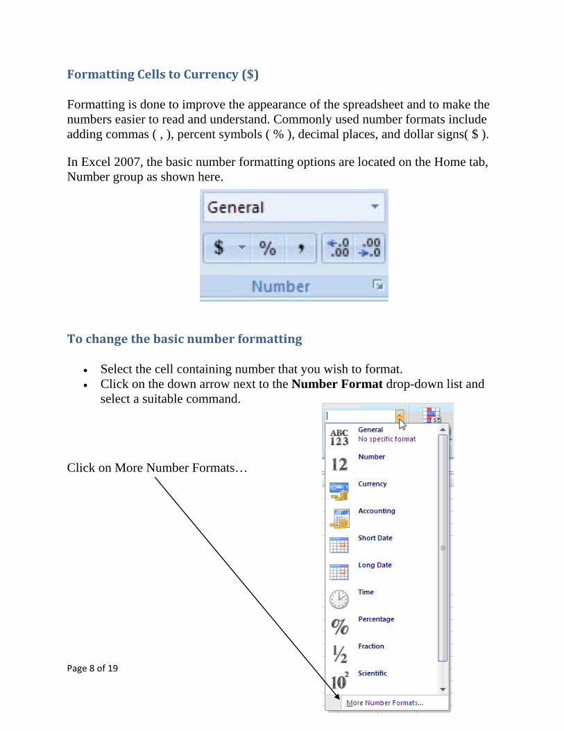
Formatting Cells to Currency ($)

Formatting is done to improve the appearance of the spreadsheet and to make the numbers easier to read and understand. Commonly used number formats include adding commas ( , ), percent symbols ( % ), decimal places, and dollar signs( $ ).

In Excel 2007, the basic number formatting options are located on the Home tab, Number group as shown here.

To change the basic number formatting

• Select the cell containing number that you wish to format. • Click on the down arrow next to the Number Format drop-down list and

select a suitable command.

Click on More Number Formats…

of 19

Charts

Charts are what we call graphs in math class. Charts are visual representations of worksheet data. Charts often make it easier to understand the data in a worksheet because users can easily pick out patterns and trends illustrated in the chart that are otherwise difficult to see.

How to create a Chart

To Create a Chart 1. Open an Excel spreadsheet with data. 2. If necessary arrange the data according to the chart to be created. 3. Highlight the desired data.

of 19

4. Select Chart Type

On the Insert Tab, in the Charts group, click the desired chart type and select the desired chart from the gallery, using the Insert Chart dialog box.

of 19

Then you could modify the chart as necessary.

Modify the Chart if necessary:

Under Design Tab

CHANGE CHART LAYOUTS

CHANGE CHART STYLES

CHANGE CHART TYPE

MOVE CHART LOCATION

SWITCH CHART DATA

of 19

Under the Layout tab

INSERT PICTURES, SHAPES OR TEXTBOXES

ADD OR REMOVE LABELS

ADD OR REMOVE AXES

CHANGE BACKGROUND

CREATE ANALYSIS

Under the Layout tab

RESET TO MATCH STYLE

CHANGE SHAPE STYLES

WORDART STYLES

ARRANGE

CHANGE SIZE

To Move a Chart 1. In an Excel workbook containing a chart, click on the chart. 2. On the Ribbon, click the Chart Tools Design contextual tab 3. In the Location group, click Move Chart to display the Move Chart Dialog

box.

of 19

Move the chart:

Move the Chart to another sheet a. In the Move Chart Dialog box, click the Object In Option. b. From the Object In drop down list, click the desired sheet. c. Click OK to Move the chart to the desired sheet.

Move the Chart to a new chart sheet a. In the Move Chart Dialog box, click the New Sheet Option. b. In the New Sheet text box, type in the desired chart sheet name c. Click OK to move the chart to the desired chart sheet.

Sorting and Filtering

Sorting Sorting Data in a Spreadsheet: You may have data in your worksheet that you would like to rearrange and display in a different sequence. Sorting is a method of

of 19

viewing data that arranges all the data into a specific order. Data can be sorted ascending order or descending order based on the alphabet or numeric information. Data can be sorted on a single criterion or multiple criteria.

To Sort Data 1. Highlight the range you want to sort, including column headings.

2. On the Data tab, in the Sort & Filter group, click on Sort.

of 19

3. In the Sort dialog box, from the Sort By drop-down list, select the column

you want to sort by. 4. If need be, from the Sort On dropdown list, click the item you want to sort

on: Values Cell Color Font Color Icon Color

5. If necessary, from the Order drop down list, select the ordering you desire. 6. If desired, click Add Level to add another sort level for a multiple level sort. 7. If necessary, from the Then By drop down list, select the column you want

to sort by. 8. If necessary, select the items you want to sort on and select the ordering you

desire.

of 19

9. Click on OK.

Filter Records

Filters works with records or rows of data in the database.

The conditions that are set are compared with one or more fields in the record. If the conditions are met, the record is displayed. If the conditions are not met, the record is filtered out so that it isn't displayed with the rest of the data records.

Filtering does not permanently remove records it just temporary hides them from view.

Use the AutoFilter feature to hide everything in a table/database except the records you want to view. Filtering displays a subset of a table, providing you with an easy way to break down your data into smaller and more manageable portions. Filtering does not rearrange your data; it simply temporarily hides rows that don't match the criteria you specify. If you wish you can sort your Filter data (to do so follow the same procedure for Sorting.)

http://spreadsheets.about.com/od/glossary/g/row_definition.htm

http://spreadsheets.about.com/od/f/g/2010-10-25-Excel-Field-Definition.htm

http://www.dummies.com/how-to/content/how-to-filter-records-in-an-excel-2010-table-with-.html#glossary-AutoFilter

of 19

1. Click inside a table, or list data and then choose Filter in the Sort & Filter group of the Data tab

Filter arrows appear beside the column headings. If the data is formatted as an Excel table, skip this step; you should already see the filter arrows.

2. Click the filter arrow beside the column heading for the column you want to filter.

Excel displays a drop-down list, which includes one of each unique entry from the selected column.

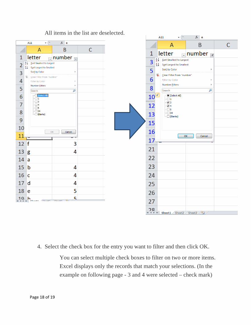
3. Remove the check mark from Select All.

http://www.dummies.com/how-to/content/how-to-filter-records-in-an-excel-2010-table-with-.html#glossary-group

http://www.dummies.com/how-to/content/how-to-filter-records-in-an-excel-2010-table-with-.html#glossary-tabs

of 19

All items in the list are deselected.

4. Select the check box for the entry you want to filter and then click OK.

You can select multiple check boxes to filter on two or more items. Excel displays only the records that match your selections. (In the example on following page - 3 and 4 were selected – check mark)

of 19

5. (Optional) Repeat Steps 2–4 as needed to apply additional filters to other columns in the filtered data.

You can apply filters to multiple columns in a table to further isolate specific items. Notice that the filter arrows on filtered columns take on a different appearance to indicate that a filter is in use.

6. To remove filters and redisplay all table data, click the Clear button on the Data tab. If multiple columns are filtered, you can click a filter arrow and select Clear Filter to remove a filter from that column only. To remove the filter arrows when you're done filtering data, choose Filter in the Sort & Filter group of the Data tab.

excel 2010: formulas and charts - john jay college of...

Documents