examining the effects of time-varying treatments or predictors daniel almirall va medical center,...
TRANSCRIPT
Examining the Effects of Time-varying Treatments or
Predictors
Daniel Almirall
VA Medical Center, Health Services Research and Development
Duke Medical Center, Department of Biostatistics
November 16, 2007
Association for Cognitive and Behavioral Therapies
Orlando, Florida

GENERAL OVERVIEW
Overview
• In this workshop we will discuss modern methods for conceptualizing and estimating the impact of treatments or predictors that vary over time– Impact of timing and sequencing of treatments
• Two classes of longitudinal causal models (developed by James Robins, Harvard) will be discussed:– Marginal Structural Models– Structural Nested Mean Models (time permitting)

Goals of this Workshop• Minimum Case Scenario (awareness)
– Spur interest in these new methods– Direct you to further reading on the subjects– Understand your data’s potential
• Hopeful Case Scenario (+ conceptual)– Understand conceptual issues & assumptions– How do these methods compare with
traditional methods• Best Case Scenario (+ technical)
– Understand the estimation techniques– Carry out estimation yourself with your data

WHAT IS THE CONTEXT?

Context: Data Source?
• The context is any observational study.• This includes data from an RCT where
initial treatment assignments are made, but patients fall into different (measured) “sequences” of treatments over time– We discuss secondary data analysis methods
• Or a classic observational study (e.g., database or retrospective study) where patients happen to be observed switching in and out of treatment(s) over time

Time-varying Treatments?• Treatment Sequencing:
– CBT: weeks 1-6; Family Therapy: weeks 8-12– CBT: weeks 1-6; no follow-up therapy
• Timing of Treatment Discontinuation– CBT for 3 weeks and none thereafter– CBT for 5 weeks and none thereafter
• Dosing of Treatment Over Time– Number of CBT “homework assignments” finished
during the CBT treatment period
• Adherence to a Full Suite of Treatments– Received full treatment during weeks 1-4– Received full treatment for the full 8 weeks

MARGINAL STRUCTURAL MODELS

Marginal Structural Models:Specific Outline
1. Motivating Example(s) (in the RCT context)
2. What is the Data Structure?
3. Formalizing Questions using MSMs
4. Primary Challenge for Data Analysis• The Nuisance of Time-varying confounders• Why traditional OLS does not work?
5. Data Analysis using Inverse-probability of Treatment Weighting
6. Miscellaneous Issues and Considerations

MOTIVATING EXAMPLE
PROSPECT Study
• RCT of a tailored primary care intervention (TPCI) for depression vs. treatment as usual (TAU)
• Subjects in the TPCI group were to meet with a depression health specialist on a regular basis
• Primary Goal of the Study: Assess the efficacy of the TPCI vs. TAU on depression and other outcomes– So-called intent to treat analysis (ITT)
• However, not all patients in the TPCI group met with their depression health specialist throughout the full course of the “treatment period”.
• Patients “switched off treatment” at different time points.
PROSPECT Study
• The variability in treatment received (in terms of meeting with health specialist) created an opportunity to ask the following question:
• Among patients in the TPCI group, what is the impact of switching off of treatment early versus later on end of study depression outcomes?– This could also be phrased as a dosing/timing
question

DATA STRUCTUREWHAT TYPE OF DATA ARE WE TALKING ABOUT?

Temporal Ordering of the DataTime, Time-varying treatments, Outcome
A1 A2
Y3
Time Interval 1 Time Interval 2 End of Study
met with health specialist or not =
1/0
met with health specialist or not =
1/0
outcome = end of study depression rating, continuous

Longitudinal Outcomes?Yes, they exist, but consider them…
A1 A2
Y3Y1 Y2
Time Interval 1 Time Interval 2 End of Study
met with health specialist or not =
1/0
met with health specialist or not =
1/0
end of study
depression ratingbaseline depression intermediate depression
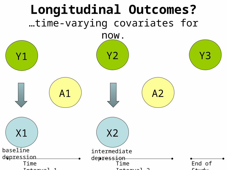
Longitudinal Outcomes?…time-varying covariates for now.
A1 A2
Y3Y1 Y2
Time Interval 1 Time Interval 2 End of Study
X1 X2
baseline depression intermediate depression

Time-varying CovariatesAlong with other baseline covariates…
X1 X2
A1 A2
Y
Time Interval 1 Time Interval 2 End of Study
baseline depression, age, race, …
intermediate depression
met with health specialist or not =
1/0
met with health specialist or not =
1/0
end of study
depression rating
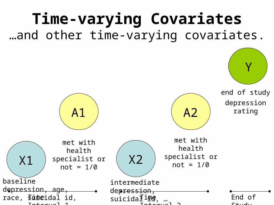
Time-varying Covariates…and other time-varying covariates.
X1 X2
A1 A2
Y
Time Interval 1 Time Interval 2 End of Study
baseline depression, age, race, suicidal id,…
intermediate depression, suicidal id, …
met with health specialist or not =
1/0
met with health specialist or not =
1/0
end of study
depression rating
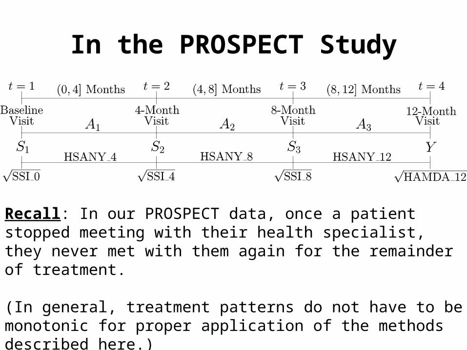
In the PROSPECT Study
Recall: In our PROSPECT data, once a patient stopped meeting with their health specialist, they never met with them again for the remainder of treatment.
(In general, treatment patterns do not have to be monotonic for proper application of the methods described here.)
FORMALIZING SCIENTIFIC QUESTIONS USING MSMs
Motivating Example: PROSPECT
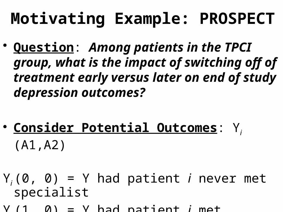
• Question: Among patients in the TPCI group, what is the impact of switching off of treatment early versus later on end of study depression outcomes?
• Consider Potential Outcomes: Yi (A1,A2)
Yi (0, 0) = Y had patient i never met specialist
Yi (1, 0) = Y had patient i met specialist once
Yi (1, 1) = Y had patient i met specialist twice

Motivating Example: PROSPECT
• Question: What is the impact of switching off of treatment early versus later on end of study depression outcomes?
• Formalize the Question Using a MSM:
E( Y (A1, A2) ) = β0 + β1 A1 + β2 A2
• β0 = E( Y(0, 0) )• β1 = E( Y(1, 0) - Y(0, 0) ) = causal effect 1• β2 = E( Y(1, 1) - Y(1, 0) ) = causal effect 2

Motivating Example: PROSPECT
• Question: What is the impact of switching off of treatment early versus later on end of study depression outcomes?
• Formalize the Question Using a MSM:
E( Y (A1, A2) ) = β0 + β1 A1 + β2 A2
• Why not just OLS regression of Y ~ [A1,A2] ?• That is, why not just fit the regression model:
E(Y | A1, A2) = β0* + β1* A1 + β2* A2 ?

THE CHALLENGE OF TIME-VARYING CONFOUNDING
When does ordinary least squares regression analysis may work? How about “adjusted” OLS regression?

Definition of a Confounder
• Loosely, a confounder is a variable that impacts subsequent treatment adoption ( assignment or receipt) and also impacts subsequent outcomes.
• However, this requires more careful thought in the time-varying setting. Why? – Because of the existence of baseline and/or time-
varying confounders; and– Because time-varying confounders may also be
outcomes of prior treatment (e.g., on the causal pathway for prior treatment).

Schematic for Effect(s) of InterestIn general: Want the effect of g(A1,A2) on EY
A1 A2
Y
Time Interval 1 Time Interval 2 End of Study
g(A1,A2) may represent a multitude of effects of interest.
met with health specialist or not =
1/0
met with health specialist or not =
1/0
end of study
depression rating

Baseline Confounders
X1
A1 A2
Y
Time Interval 1 Time Interval 2 End of Study
met with health specialist or not =
1/0
met with health specialist or not =
1/0
end of study
depression rating
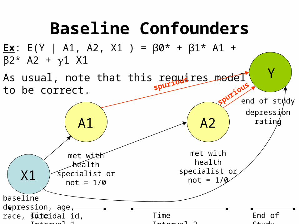
Adjusting for X1 in ordinary regression is a legitimate strategy in this case.
spurious
spurious
baseline depression, age, race, suicidal id,…

Baseline Confounders
X1
A1 A2
Y
Time Interval 1 Time Interval 2 End of Study
met with health specialist or not =
1/0
met with health specialist or not =
1/0
end of study
depression rating
Ex: Fit the following model by OLS
E(Y | A1, A2, X1 ) = β0* + β1* A1 + β2* A2 + X1
spurious
spurious
baseline depression, age, race, suicidal id,…
Baseline Confounders
X1
A1 A2
Y
Time Interval 1 Time Interval 2 End of Study
met with health specialist or not =
1/0
met with health specialist or not =
1/0
end of study
depression rating
Ex: E(Y | A1, A2, X1 ) = β0* + β1* A1 + β2* A2 + 1 X1
As usual, note that this requires model to be correct.
spurious
spurious
baseline depression, age, race, suicidal id,…
Time-varying Confounders
X1 X2
A1 A2
Y
Time Interval 1 Time Interval 2 End of Study
met with health specialist or not =
1/0
met with health specialist or not =
1/0
end of study
depression rating
baseline depression, age, race, suicidal id,…
intermediate depression, suicidal id, …
spurious
spurious
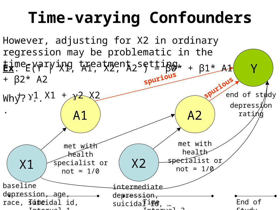
However, adjusting for X2 in ordinary regression may be problematic in the time-varying treatment setting.
Why? ...
Ex: E(Y | X1, A1, X2, A2 ) = β0* + β1* A1 + β2* A2
+ 1 X1 + 2 X2

First ProblemWith conditioning on (or “adjusting”) X2 in OLS.
X2
A1 A2
Y
Time Interval 1 Time Interval 2 End of Study
Xcut o
ffmet with health specialist or not =
1/0
end of study
depression rating
intermediate depression, suicidal id, …
Second Problem
X2
A1 A2
Time Interval 1 Time Interval 2 End of Study
U
spurious non-causal path
met with health specialist or not =
1/0
end of study
depression rating
intermediate depression, suicidal id, …
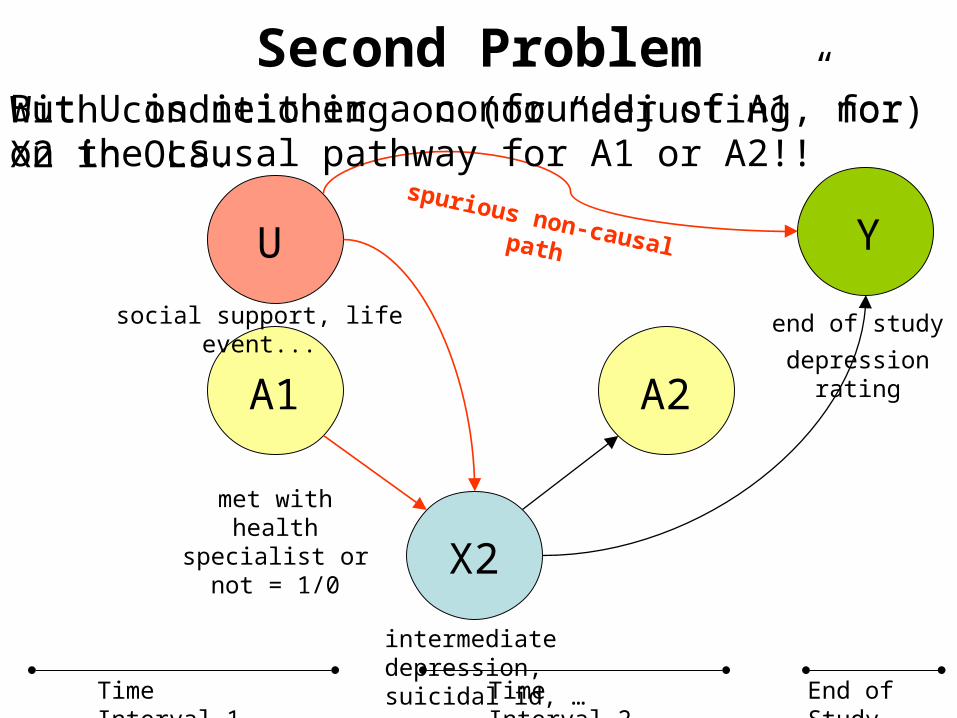
social support, life event...
But U is neither a confounder of A1, nor on the causal pathway for A1 or A2!!With conditioning on (or “adjusting” for) X2 in OLS.
Y

Second Problem
X2
A1 A2
Time Interval 1 Time Interval 2 End of Study
U
spurious non-causal path
met with health specialist or not =
1/0
end of study
depression rating
outside therapy, …
income, social support, …
Given outside therapy, we will see that meeting with health specialist decreases end-of-study depression.
+
-
-
Y

Second Problem
X2
A1 A2
Time Interval 1 Time Interval 2 End of Study
U
spurious non-causal path
met with health specialist or not =
1/0
end of study
depression rating
outside therapy, …
income, social support, …
But …
+
-
-
Y

So what can we do to overcome?What is the alternative to “OLS adjustment” ?
X1 X2
A1 A2
Time Interval 1 Time Interval 2 End of Study
XX
That eliminate/reduce confounding in the sample.Requires that we have all confounders of A1 and A2.
Weights: function of Pr(A1| X1) and Pr(A2| X1, A1, X2).
X
Does not require knowledge about U.
Y

ESTIMATING MSMs USING INVERSE-PROBABILITY-OF-TREATMENT WEIGHTINGNow Entering … “doer of deeds” section of the workshop

Inverse-Probability Weighting?
• Sometimes known as “propensity score weighting” methodology
• Related to the Horvitz-Thompson Estimator – see the Survey Sampling / Demography
literature• To make ideas concrete, we first consider
how to do it in the one-time point setting.• Then we see how these ideas can be
extended to the time-varying setting.

IPT Weighting Tutorial(non-time-varying setting)
• X is a confounder of the effect of the
effect of A on Y.
X
A
Y
met with health specialist or not =
y/n
end of study
depression
severe baseline depression = y/n
+ +
• Ex: Patients more depressed at
baseline may be more likely to
meet with their HS.• Ex: They may also be
more likely to be
depressed later.

ORIGINALDATA
Met with HS = YES
Met with HS = NO
Sev. Base. Depression = YES
60 30Sev. Base. Depression = NO
20 40
IPT Weighting Tutorial(non-time-varying setting)
• X is a confounder of the effect of the
effect of A on Y.• Suppose we have a data set
with N = 150 subjects
X
A
Y
met with health specialist or not =
y/n
end of study
depression
severe baseline depression = y/n
+
ORIGINALDATA
Met with HS = YES
Met with HS = NO
Sev. Base. Depression = YES
60 30Sev. Base. Depression = NO
20 40
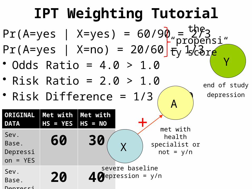
IPT Weighting TutorialPr(A=yes | X=yes) = 60/90 = 2/3
Pr(A=yes | X=no) = 20/60 = 1/3• Odds Ratio = 4.0 > 1.0• Risk Ratio = 2.0 > 1.0• Risk Difference = 1/3 > 0.0
X
A
Y
met with health specialist or not =
y/n
end of study
depression
severe baseline depression = y/n
+
the “propensity
score”

ORIGINALDATA
Met with HS = YES
Met with HS = NO
Sev. Base. Depression = YES
60 30Sev. Base. Depression = NO
20 40
IPT Weighting Tutorial• The basic idea behind IPT weighting is
to use the information in the propensity score to undo the association between the confounder(s) X and the primary “treatment” variable A
• How?
X
A
Y
met with health specialist or not =
y/n
end of study
depression
severe baseline depression = y/n
+

WEIGHTED DATA
Met with HS = YES
Met with HS = NO
Sev. Base. Depression = YES
60 30Sev. Base. Depression = NO
20 40
IPT Weighting TutorialPr(A=yes | X=yes) = 60/90 = 2/3
Pr(A=yes | X=no) = 20/60 = 1/3
Pi = 2/3 Xi + 1/3 (1-Xi) = propensity score
Assign the following weights
Wi = Ai / Pi + (1-Ai) / (1-Pi)
X
A
Y
met with health specialist or not =
y/n
end of study
depression
severe baseline depression = y/n
+
the “propensity
score”

IPT Weighting TutorialPi = 2/3 Xi + 1/3 (1-Xi) = propensity score
Assign the weights
Wi = Ai / Pi + (1-Ai) / (1-Pi)
Does this really work? Yes. Take a
look at the “weighted table”:
X
A
Y
met with health specialist or not =
y/n
end of study
depression
severe baseline depression = y/n
WEIGHTED DATA
Met with HS = YES
Met with HS = NO
Sev. Base. Depression = YES
60*3/2= 90
30*3= 90
Sev. Base. Depression = NO
20*3= 60
40*3/2= 60
X
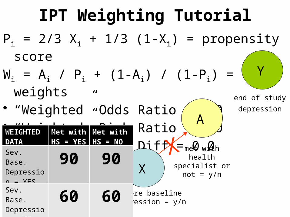
IPT Weighting TutorialPi = 2/3 Xi + 1/3 (1-Xi) = propensity score
Wi = Ai / Pi + (1-Ai) / (1-Pi) = weights
• “Weighted” Odds Ratio = 1.0• “Weighted” Risk Ratio = 1.0• “Weighted” Risk Diff = 0.0
X
A
Y
met with health specialist or not =
y/n
end of study
depression
severe baseline depression = y/n
WEIGHTEDDATA
Met with HS = YES
Met with HS = NO
Sev. Base. Depression = YES
90 90Sev. Base. Depression = NO
60 60
X

IPT Weighting Tutorial• The final step is to model the effect of A on Y
just as you would (e.g., linear regression),
but using the weighted sample.• One way to do this is weighted
ordinary least squares.• Ex: E(Y | A) =W= β0* + β1* A• No need to adjust
for X in the actual
regression modelX
A
Y
met with health specialist or not =
y/n
end of study
depression
severe baseline depression = y/n
X
β1
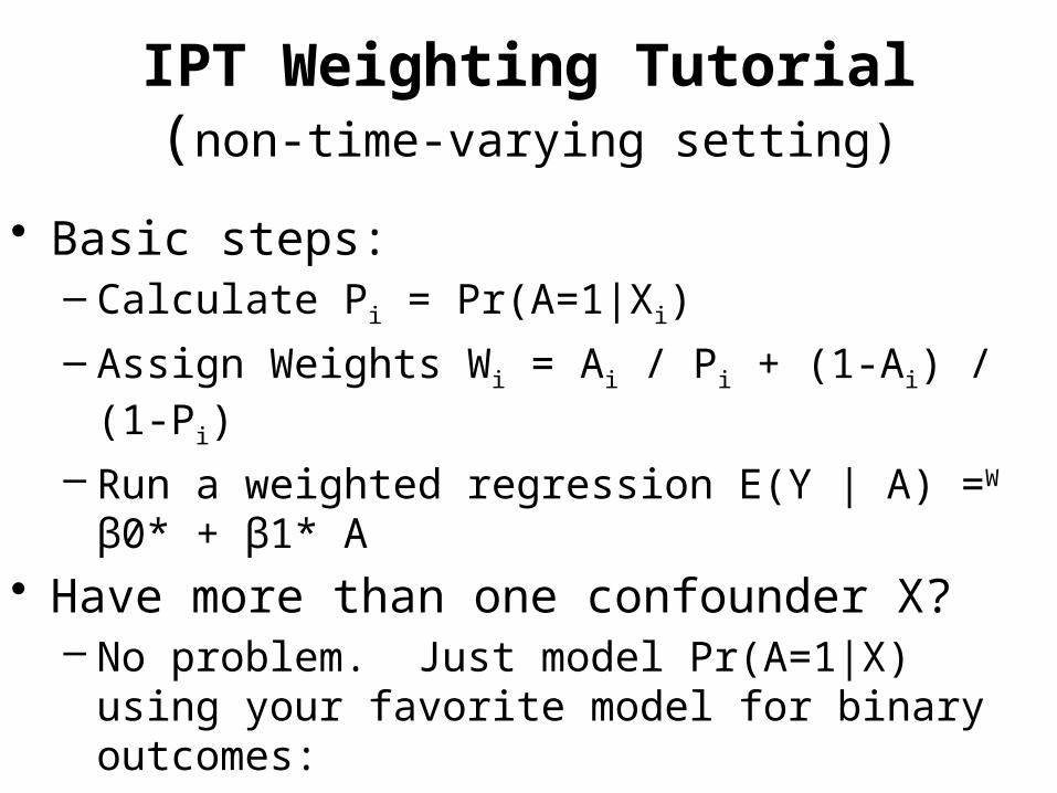
IPT Weighting Tutorial(non-time-varying setting)
• Basic steps:– Calculate Pi = Pr(A=1|Xi)
– Assign Weights Wi = Ai / Pi + (1-Ai) / (1-Pi)
– Run a weighted regression E(Y | A) =W β0* + β1* A• Have more than one confounder X?
– No problem. Just model Pr(A=1|X) using your favorite model for binary outcomes:
– Logistic regression model, probit models, or generalized boosting models (GBM)• GBM: see McCaffrey et al 2004, Psych Methods

IPT Weighting Tutorial(non-time-varying setting)
• Under what assumptions does the estimate of β1* in the weighted least squares regression
E(Y | A) =W= β0* + β1* A
identify the causal effect β1 from the MSM
E(Y(A)) = β0 + β1 A
1.SUTVA (Consistency): Y = Y(1)*A + Y(0)*(1-A)
2.Pi bounded away from 0 and 1
3.Ignorability Assumption
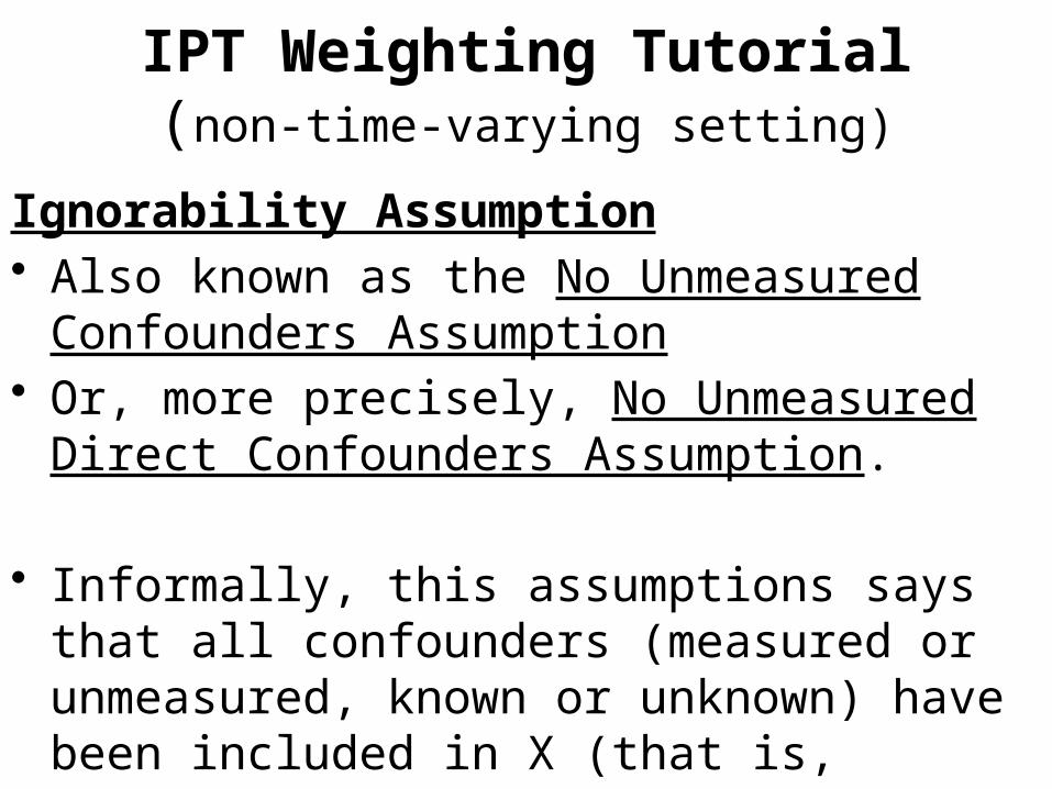
IPT Weighting Tutorial(non-time-varying setting)
Ignorability Assumption• Also known as the No Unmeasured
Confounders Assumption• Or, more precisely, No Unmeasured Direct
Confounders Assumption.
• Informally, this assumptions says that all confounders (measured or unmeasured, known or unknown) have been included in X (that is, accounted, or adjusted, for).

IPTW in the Time-varying Setting• Remember our Goal: Estimate the MSM
E(Y(A1,A2)) = β0 + β1 A1 + β2 A2
But…
X1 X2
A1 A2
Time Interval 1 Time Interval 2 End of Study
Y

IPTW in the Time-varying SettingGoal: E(Y(A1,A2)) = β0 + β1 A1 + β2 A2• But … how do we eliminate the red
arrows? Using a IP weighting scheme.
X1 X2
A1 A2
Time Interval 1 Time Interval 2 End of Study
XX X
Y

IPTW in the Time-varying Setting
Multiple Propensity Score Models (@ each t)• Model P1 = Pr(A1=1|X1) and• Model P2 = Pr(A2=1|X1,A1,X2)
Assign Inverse Prob. Weights (@ each t)• Assign W1 = A1/P1 + (1-A1) / (1-P1)• Assign W2 = A2/P2 + (1-A2) / (1-P2)
Assign Overall Weights• W = W1 * W2 (each person has 1 weight)
Run a weighted least squares regression:• E(Y | A1,A2) =W= β0* + β1* A1 + β2* A2
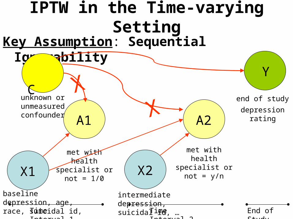
IPTW in the Time-varying Setting
Key Assumption: Sequential Ignorability
X2
A1 A2
Time Interval 1 Time Interval 2 End of Study
C
met with health specialist or not =
1/0
end of study
depression rating
intermediate depression, suicidal id, …
unknown or unmeasured confounder
Y
X1
baseline depression, age, race, suicidal id,…
met with health specialist or not =
y/n
XX

IPTW in the Time-varying Setting
Key Assumption: C (baseline or time-varying) does not exist.
X2
A1 A2
Time Interval 1 Time Interval 2 End of Study
C
met with health specialist or not =
1/0
end of study
depression rating
intermediate depression, suicidal id, …
unknown or unmeasured confounder
Y
X1
baseline depression, age, race, suicidal id,…
met with health specialist or not =
y/n

IPT WEIGHTING IN PRACTICE

Actual Steps: IPT Weighting in the Time-Varying Setting
1. Specify the scientific question using the MSM
2. Run Unadjusted Ordinary Least Squares Analysis
At each time point t :
3. Examine Initial (Im)balance (Assess Measured Confounding)
4. Build Propensity Score Pt
5. Calculate Weights Wt and Examine Its Distribution
6. Re-Examine Balance at t Using the Wt Weighted Sample
7. Repeat Steps 4-6 Until Achieve Desired Balance
End loop over t .
8. Calculate Final Weights W = t Wt
9. Run Weighted Least Squares Analysis (Use Robust SEs)
10. Compare Results in 9 with Results in 2 and Comment/Discuss

A WORKED EXAMPLE USING SIMULATED (COMPUTER GENERATED) DATA
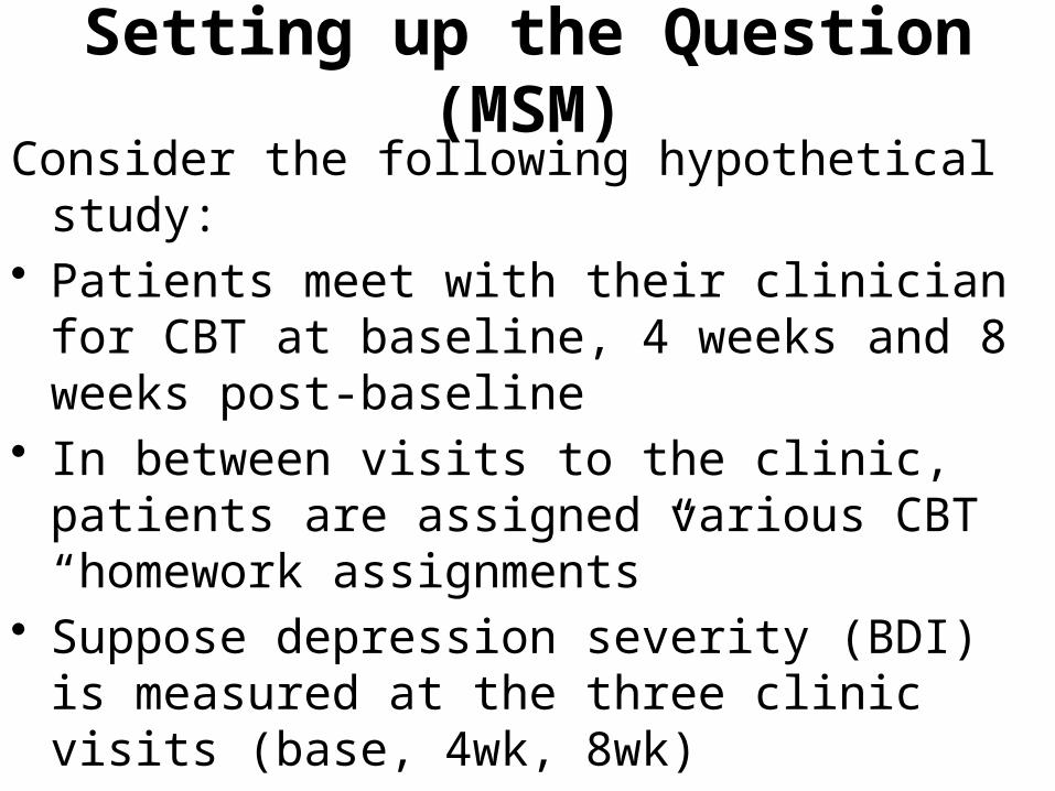
Setting up the Question (MSM)Consider the following hypothetical study:• Patients meet with their clinician for CBT at
baseline, 4 weeks and 8 weeks post-baseline• In between visits to the clinic, patients are
assigned various CBT “homework assignments”
• Suppose depression severity (BDI) is measured at the three clinic visits (base, 4wk, 8wk)
• Suppose we have measured whether or not patients completed their homework in the two intervals between clinic visits (0-4wk, 4-8wk).

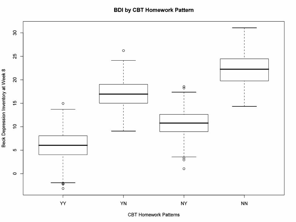
Setting up the Question (MSM)• Let Y = BDI8• Let A1 and A2 denote the binary variables
indicating whether HW was completed (0/1=n/y)• Our goal is to understand the impact of patterns
of CBT homework completion (over the two intervening intervals) on depression severity outcomes at 8 weeks.
• Our MSM is a simple one:
E(Y(A1,A2)) = β0 + β1 A1 + β2 A2 + β3 A1 A2

Setting up the Question (MSM)• Our MSM is a simple one:
E(Y(A1,A2)) = β0 + β1 A1 + β2 A2 + β3 A1 A2• β0 = E [Y(0,0)]• β1 = E [Y(1,0) - Y(0,0)]• β2 = E [Y(0,1) - Y(0,0)]• β1 + β2 + β3 = E [Y(1,1) - Y(0,0)]• β3 = E [Y(1,1) - Y(1,0)] - E [Y(0,1) - Y(0,0)]
The most important confounder is previous levels of depression; that is, previous BDI scores.


FINAL REMARKS

Separability?• What if for particular levels of a covariate (or
combination of covariates) all patients receive the same treatment?– Think “regression discontinuity design” for intuition
• In this case, inverse-probability of treatment weighting does not work.– E.g., Cannot create the propensity score models.
• In this case, we must rely on models for the outcome for covariate “adjustment” and propensity score methods are less useful.

Design RecommendationsWhat if you are planning a study like this?
Key Step 1: Clear Sense of Scientific Question, MSM• Clear definition of time-varying treatment• How time is defined becomes important• Alignment of time, time-varying treatments, and Y
Key Step 2: Make Sequential Ignorability Plausible• Brainstorm and measure most important factors
affecting your time-varying predictor or treatment– What are all baseline and time-varying variables that
determine whether patient will meet with Health Specialist?
Both of these informed heavily by a well-developed conceptual model or theoretical framework

Baseline Conditional MSMsCan we condition on X1 (and/or other
baseline variables) in the MSM?• Yes. For example, the following MSM:
E(Y(A1,A2) | V)
= β0 + β1 A1 + β2 A2 + β3 A1 A2 + V
• For example: V = Age, race, gender, BDI0• Suppose V is a subset of X1• This is still a MSM.

Baseline Conditional MSMsE(Y(A1,A2) | V)
= β0 + β1 A1 + β2 A2 + β3 A1 A2 + V• Model specification (model fit) is important• Adjusting for baseline covariates may increase
precision = smaller standard errors• Use “stabilized weights” with a numerator that
reflects adjustment for baseline covariates– Stabilized Weights (recall V is a subset of X1)
W1 = P(A1 | V) / P(A1| X1)W2 = P(A2 | V,A1) / P(A2| X1,A1,X2)
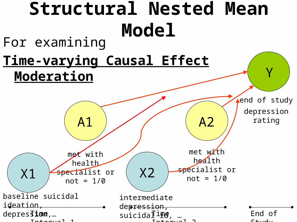
Structural Nested Mean ModelFor examining
Time-varying Causal Effect Moderation
X1 X2
A1 A2
Y
Time Interval 1 Time Interval 2 End of Study
met with health specialist or not =
1/0
met with health specialist or not =
1/0
end of study
depression rating
baseline suicidal ideation, depression,…
intermediate depression, suicidal id, …

Structural Nested Mean ModelWe will do this next time we meet…
X1 X2
A1 A2
Y
Time Interval 1 Time Interval 2 End of Study
met with health specialist or not =
1/0
met with health specialist or not =
1/0
end of study
depression rating
baseline suicidal ideation, depression,…
intermediate depression, suicidal id, …

References
• Robins. (1999). Association, causation, and marginal structural models. Synthese, 121:151-179.– A classic, well-written, paper introducing the MSM and IPT Weighting
• Hernán, Brumback, Robins. (2001). Marginal structural models to estimate the joint causal effect of nonrandomized treatments. Journal of the American Statistical Association, 96(454):440-448.
• Robins, Hernán, Brumback. (2000). Marginal structural models and causal inference in epidemiology. Epidemiology, September 11(5):550-560. – Two excellent papers by describing the MSM and IPT Weighting: the
primary motivation here are epidemiologic studies• Bray, Almirall, Zimmerman, Lynam & Murphy(2006).
Assessing the Total Effect of Time-varying Predictors in Prevention Research. Prevention Science 7(1):1-17. – This paper looks at the MSM and IPT Weighting when the primary
analysis model is a Discrete-time Survival Analysis.

References• McCaffrey, et al (2004).
Propensity score estimation with boosted regression for evaluating causal effects in observational studies. Psychological Methods. 9(4)– This is an excellent paper describing propensity score weighting in one
time point. The authors describe a modern method, boosting, for calculating the propensity score. Substance abuse application.
• Almirall, Ten Have, Murphy(2006). Structural nested mean models for time-varying effect moderation. Forthcoming. – This paper describes the SNMM for assessing time-varying causal effect
moderation and introduces a simple to use 2-stage regression estimator for the SNMM and compares it to the classic estimator, the G-Estimator. The motivating application in this paper is the PROSPECT study mentioned earlier in these slides.
• Almirall, Coffman, Yancy, Murphy(2006). Maximum likelihood estimation of the structural nested mean model using SAS PROC NLP. Forthcoming in a book entitled “Analysis of Observational Health-Care Data Using SAS”.– This book chapter describes how to implement a maximum likelihood
estimator of the SNMM using SAS PROC NLP. In this chapter we examine time-varying moderators (e.g., compliance to diet, exercise) of the impact of weight loss (time-varying) on health-related quality of life.

Thank you.