1

Exact Coherent Structures in Pipe Flow: TravellingWave Solutions

H. Wedin & R.R. Kerswell†

Department of Mathematics, University of Bristol,Bristol, BS8 1TW, England, UK

27 February 2004

ABSTRACT

Three-dimensional travelling wave solutions are found for pressure-driven fluid flowthrough a circular pipe. They consist of three well-defined flow features - streamwiserolls and streaks which dominate and streamwise-dependent wavy structures. The trav-elling waves can be classified by the m-fold rotational symmetry they possess about thepipe axis with m = 1, 2, 3, 4, 5 and 6 solutions identified. All are born out of saddle nodebifurcations with the lowest corresponding to m = 3 and traceable down to a Reynoldsnumber (based on the mean velocity) of 1251. The new solutions are found using a con-structive continuation procedure based upon key physical mechanisms thought generic towall-bounded shear flows. It is believed the appearance of these new alternative solutionsto the governing equations as the Reynolds number is increased is a necessary precursorto the turbulent transition observed in experiments.

1. Introduction

The stability of pressure-driven flow through a long circular pipe is one of the mostclassical and intriguing problems in fluid mechanics. Ever since the original experimentsof Reynolds (1883), it has been known that the steady, unidirectional Hagen-Poiseuilleflow, uniquely realised at low Reynolds numbers Re, can undergo transition to turbu-lence when disturbed sufficiently strongly at high enough Reynolds numbers. Subsequentexperimental work has confirmed and extended Reynolds’s first observations to studyhow transition occurs and the subsequent possibly intermittent turbulent state (Wyg-nanski & Champagne 1973, Wygnanski et al. 1975, Darbyshire & Mullin 1995, Draadet al. 1998, Eliahou et al. 1998, Han et al. 2000, Hof et al. 2003). What consistentlyemerges is the sensitivity of the transition onset to the exact form of the perturbationand how the size of the threshold amplitude required to trigger transition decreases withincreasing Reynolds number (Darbyshire & Mullin 1995, Hof et al. 2003). The fact thatthis unidirectional flow is believed linearly stable (Lessen et al. 1968, Garg & Rouleau1972, Salwen et al. 1980, Herron 1991, Meseguer & Trefethen 2003) has served only tohighlight the essentially nonlinear origin of the observed transition. Pipe flow is then justone of a class of wall-bounded shear flows which suffer turbulent transition through aprocess or processes unrelated to the local stability properties of the low-Reynolds basicsolution. Further examples include plane Couette flow where the basic solution has beenproved linearly stable (Romanov 1973) as well as plane Poiseuille flow where the baseflow loses stability at a far higher Reynolds number (Re = 5772) than that at whichtransition is observed (Re ≈ 2100 Rozhdestvensky & Simakin 1984, Re ≈ 2300 Keefe et

† email: R.R.Kerswell@bris.ac.uk

2

al. 1992 or using a Reynolds based on the centreline velocity ≈ 1000 Carlson et al. 1982).

Recent thinking now views transition in these systems as being an issue revolvingaround the existence of other solutions that do not have any connection with the basicflow, and their basins of attraction. Pipe flow can be considered as a nonlinear dy-namical system du/dt = f (u; Re) defined by the governing Navier-Stokes equationstogether with the appropriate pressure-gradient forcing and boundary conditions, andRe parametrising the system. Within this framework, there is one linearly-stable fixedpoint (Hagen-Poiseuille flow) for all Re which is a global attractor for Re < Reg (non-linearly stable) but only a local attractor for Re > Reg (nonlinearly unstable but stilllinearly stable). It is known that all disturbances to this basic state must decay ex-ponentially if Re < Ree = 81.49 (Joseph & Carmi 1969), the energy stability limit,whereas for Ree ≤ Re < Reg, some disturbances can transiently grow but then decay(Boberg & Brosa 1988, Bergstrom 1993, Schmid & Henningson 1994, O’Sullivan & Breuer1994, Zikanov 1996). At Re = Reg, new limit sets in phase space (typically steady orperiodic solutions to the Navier-Stokes equations) are now presumed born which sup-port the complex dynamics observed at transition. These new solutions are imagined asproviding the skeleton about which complicated time-dependent orbits observed in tran-sition may drape themselves so that they no longer evolve back to Hagen-Poiseuille flowat long times (Schmiegel & Eckhardt 1997, Eckhardt et al. 2002). As a result, the emer-gence of these alternative solutions is believed to bear a strong relation with the observedlower limit where turbulence is sustainable of Ret ≈ 1800− 2000 and their existence tostructure the transition process itself. The fact that the basic steady solution remains alocal attractor in phase space is largely secondary to the fact that its basin of attractiondiminishes rapidly as Re increases. This, taken with the fact that the basin boundary isundoubtedly complicated in such a high dimensional phase space, explains why the (lami-nar) Hagen-Poiseuille solution is so sensitive to the size and form of an initial disturbance.

The existence of alternative solutions to the Navier-Stokes equations has now beendemonstrated in a number of different wall-bounded shear flows (and sometimes clearlyobserved, e.g. Anson et al. 1989). Steady solutions have been found in plane Couette flowdown to Re = 125 (Nagata 1990, Clever & Busse 1997 or more accurately Re = 127.7,Waleffe 2003) compared to a transitional value of Re ≈ 320 − 350 (Lundbladh & Jo-hansson 1991, Tillmark & Alfredsson 1992, Daviaud et al. 1992, Dauchot & Daviaud1995, Bottin et al. 1998), and travelling wave solutions in plane Poiseuille flow at Re = 977(Waleffe 2003) compared to a transitional value of Re ≈ 2100 − 2300 (Rozhdestvensky& Simakin 1984, Keefe et al. 1992). What is striking is how the key structural featuresof these solutions - strong downstream vortices and streaks - coincide with what is ob-served in experiments as transient coherent structures. The clear implication seems tobe that these solutions are saddles in phase space so that the flow dynamics can residetemporarily in their vicinity (the flow approaches near to these solutions in phase spacevia the stable manifold before being flung away in the direction of the unstable mani-fold). Given this success, there has been a concerted effort to theoretically find solutionsother than the Hagen-Poiseuille state in pipe flow. Despite some suggestive asymptoticanalyses (Davey & Nguyen 1971, Smith & Bodonyi 1982, Walton 2002), no non-trivialsolutions have so far been reported (Patera & Orszag 1981, Landman 1990a,b).

The standard approach to finding such nonlinear solutions is homotopy which wasused by Nagata (1990) to find the first disconnected solutions in plane Couette flow.This continuation approach relies on the presence of a neighbouring problem in which

3

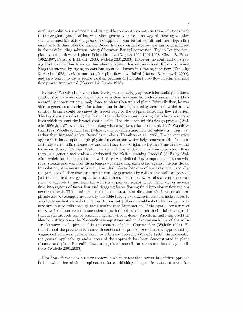
nonlinear solutions are known and being able to smoothly continue these solutions backto the original system of interest. Since generally there is no way of knowing whethersuch a connection exists a priori, the approach can be rather hit-and-miss dependingmore on luck than physical insight. Nevertheless, considerable success has been achievedin the past building solution ‘bridges’ between Benard convection, Taylor-Couette flow,plane Couette flow and plane Poiseuille flow (Nagata 1990,1997,1998, Clever & Busse1992,1997, Faisst & Eckhardt 2000, Waleffe 2001,2003). However, no continuation strat-egy back to pipe flow from another physical system has yet succeeded. Efforts to repeatNagata’s success by trying to continue solutions known in rotating pipe flow (Toplosky& Akylas 1988) back to non-rotating pipe flow have failed (Barnes & Kerswell 2000),and an attempt to use a geometrical embedding of (circular) pipe flow in elliptical pipeflow proved impractical (Kerswell & Davey 1996).

Recently, Waleffe (1998,2003) has developed a homotopy approach for finding nonlinearsolutions to wall-bounded shear flows with clear mechanistic underpinnings. By addinga carefully chosen artificial body force to plane Couette and plane Poiseuille flow, he wasable to generate a nearby bifurcation point in the augmented system from which a newsolution branch could be smoothly traced back to the original zero-force flow situation.The key steps are selecting the form of the body force and choosing the bifurcation pointfrom which to start the branch continuation. The ideas behind this design process (Wal-effe 1995a,b,1997) were developed along with coworkers (Hamilton et al. 1995, Waleffe &Kim 1997, Waleffe & Kim 1998) while trying to understand how turbulence is maintained

rather than initiated at low Reynolds numbers (Hamilton et al. 1995). The continuationapproach is based upon simple physical mechanisms which help remove much of the un-certainty surrounding homotopy and can trace their origins to Benney’s mean-flow firstharmonic theory (Benney 1984). The central idea is that in wall-bounded shear flowsthere is a generic mechanism - christened the ‘Self-Sustaining Process’ (SSP) by Wal-effe - which can lead to solutions with three well-defined flow components - streamwiserolls, streaks and wavelike disturbances - maintaining each other against viscous decay.In isolation, streamwise rolls would secularly decay because of viscosity but, crucially,the presence of other flow structures naturally generated by rolls near a wall can providejust the required energy input to sustain them. The streamwise rolls advect the meanshear alternately to and from the wall (in a spanwise sense) hence lifting slower movingfluid into regions of faster flow and dragging faster flowing fluid into slower flow regionsnearer the wall. This produces streaks in the streamwise direction which at certain am-plitude and wavelength are linearly unstable through spanwise-inflexional instabilities toaxially-dependent wave disturbances. Importantly, these wavelike disturbances can drivenew streamwise rolls through their nonlinear self-interaction. If the spatial structure ofthe wavelike disturbances is such that these induced rolls match the initial driving rollsthen the initial rolls can be sustained against viscous decay. Waleffe initially explored thisidea by cutting open the Navier-Stokes equations and confirming each link of the rolls-streaks-waves cycle piecemeal in the context of plane Couette flow (Waleffe 1997). Hethen turned the process into a smooth continuation procedure so that the approximatelyengineered solutions became exact to arbitrary accuracy (Waleffe 1998). Subsequently,the general applicability and success of the approach has been demonstrated in planeCouette and plane Poiseuille flows using either non-slip or stress-free boundary condi-tions (Waleffe 2001,2003).

Pipe flow offers an obvious new context in which to test the universality of this approachfurther which has obvious implications for establishing the generic nature of transition

4

in wall-bounded shear flows. Also this approach offers a promising new technique to findalternative nonlinear solutions which have proved so enigmatic in this particular prob-lem. As a result the objectives of this paper are twofold: to establish the credentials ofthis constructive approach and, perhaps only marginally more importantly, to find thesolutions themselves.

The plan of the paper is as follows. Section 2 introduces the pipe flow problem, statesthe governing equations and makes some important definitions. Section 3 discusses theSelf-Sustaining Process (SSP) and illustrates how it may be used to find approximatesolutions to the governing equations. Although these ‘solutions’ are not exact since cer-tain terms in the equations are ignored, it appears that all the important terms havebeen retained by appealing to the correct physical mechanisms. As a result, each such‘approximate’ solution has a high probability of leading to an exact counterpart via asmooth continuation procedure. Section 4 shows how this can be done to arbitrary accu-racy using the information gleaned from settling up a SSP ‘solution’. Section 5 collectstogether all the results of the paper before a discussion follows in section 6.

While this work was being completed we became aware that Faisst & Eckhardt (2003)had just isolated converged twofold and threefold rotationally symmetric solutions (RRR2

and RRR3 waves as defined in (2.12) below) in pipe flow using a similar continuation ap-proach. Here we confirm these findings, discover new branches of the threefold rotationallysymmetric (RRR3) waves and present converged onefold, fourfold, fivefold and sixfold rota-tionally symmetric (RRR1, RRR4, RRR5 and RRR6) waves solutions for the first time. This paperthen complements and extends their study as well as discussing why the continuationapproach works.

2. Governing Equations

We consider an incompressible fluid of constant density ρ and kinematic viscosity νflowing in a circular pipe of radius s0 under the action of a constant applied pressuregradient

∇p∗ = −4ρνW

s20

z. (2.1)

At low enough values of the Reynolds number Re := s0W/ν, the realised flow is uniquelyHagen-Poiseuille flow (HPF)

u∗ = W

(1 −

s2

s20

)z, (2.2)

in the usual cylindrical polar coordinate system (s, φ, z). The governing equations (non-dimensionalised using the Hagen-Poiseuille centreline speed W and pipe radius s0) forpipe flow are

∂u

∂t+ u.∇u + ∇p =

1

Re∇2u +

4

Rez, (2.3)

∇.u = 0, (2.4)

with boundary condition

u(1, φ, z) = 0 (2.5)

5

where u = u∗/W and p represents the pressure deviation away from the imposed gradi-ent. A mean Reynolds number can be defined in terms of the mean speed

W :=1

π

∫ 2π

0

dφ

∫ 1

0

sds u∗.z (2.6)

of the fluid down the pipe

Rem :=2s0W

ν(2.7)

and in contrast to the pressure-gradient Reynolds number Re, is not known a priori.The extent to which Rem and Re differ is a useful measure of how far the realised flowsolution has deviated from HPF, u = (1 − s2)z, where they are identical. The energydissipation rate per unit mass is

D :=1

πRelim

L→∞

1

2L

∫ L

−L

dz

∫ 2π

0

dφ

∫ 1

0

sds|∇u|2 =2Rem

Re2(2.8)

in units of W 3/s0 and the friction coefficient (Schlichting 1968, eqn(5.10)) is defined as

Λ :=1

ρ

dp

dz

/1

4s0W

2=

64Re

Re2m

. (2.9)

Computationally, it is preferable to work with the ‘perturbation’ velocity away fromHagen-Poiseuille flow, that is, u := u −

(1 − s2

)z which then satisfies homogeneous

boundary conditions at the pipe wall and is presumed periodic along the pipe. Thepressure p is already the ‘perturbation’ pressure and is strictly periodic to keep theapplied pressure gradient fixed. The governing equations, (2.3) and (2.4), rewritten forthese new variables and used henceforth are

∂u

∂t+ (1 − s2)

∂u

∂z− 2su z + u.∇u + ∇p −

1

Re∇2u = 0, (2.10)

∇.u = 0. (2.11)

The nonlinear solutions found in this paper take the form of travelling waves whichpropagate at a constant speed and are therefore steady in an appropriate Galilean frame.This speed is expected to be non-zero due to the lack of fore-aft symmetry in pipeflow and represents an unknown emerging like an eigenvalue as part of the solutionprocedure. The travelling waves also possess a number of symmetries, the most importantof which is a discrete m-fold rotational symmetry in the azimuthal direction φ so thatthe transformation

RRRm : (u, v, w, p)(s, φ, z) → (u, v, w, p)(s, φ + 2π/m, z) (2.12)

(in the usual cylindrical coordinates) leaves them unchanged for some integer m. Thisprovides a natural partitioning and henceforth we shall refer to travelling waves withRRRm symmetry as simply RRRm−waves. Properties of RRRm−waves with m = 1, 2, 3, 4, 5 & 6will be described below but special attention will be devoted to illustrating how RRR2 &RRR3−waves were found since these appear first as Re increases.

3. The Self-Sustaining Process (SSP)

There are three physical mechanisms and three distinct active velocity structures whichcome together to produce a self-sustained cycle. We look for a travelling wave solutionor equivalently a steady solution in a frame moving at some constant speed c in the

6

streamwise z direction. In this Galilean frame, a steady velocity field and pressure fieldcan be decomposed without loss of generality into three parts

[u

p

]=

U(s, φ)V (s, φ)0P (s, φ)

rolls

+

00W (s, φ)0

streaks

+

u(s, φ, z)v(s, φ, z)w(s, φ, z)p(s, φ, z)

waves

(3.1)

where the various streamwise-independent and streamwise-dependent parts have beenlabelled ‘rolls’, ‘streaks’ and ‘waves’ respectively. For uniqueness, the waves have nomean under streamwise averaging, that is, u

z= U where

( )z

:= limL→∞

1

2L

∫ L

−L

( ) dz. (3.2)

Also formally, the term ‘streak’ usually refers to a fluctuation in the streamwise velocityaway from a mean, W (s, φ) − W (s) (where W (s) is the azimuthally-averaged velocity).Here, as a convenient shorthand we refer to the whole spanwise modulated shear flowW (s, φ) created by the rolls as the streak field.

In the absence of z-dependent waves, the streamwise rolls, [U(s, φ), V (s, φ), 0], have noenergy source and will secularly decay under viscosity. However before this can happen,they redistribute the mean shear to produce streaks, W (s, φ). This involves a considerableamplification in the overall disturbance to the flow, a general phenomenon in shear flowswhich has become known as ‘transient growth’ (Boberg & Brosa 1988, Bergstrom 1993,Schmid & Henningson 1994, O’Sullivan & Breuer 1994, Zikanov 1996). The process issimple to understand and linear in nature depending only on the slow advection across alarge mean shear sustained for a long time. In particular, if the streamwise rolls initiallyhave amplitude ε � 1, their viscous decay rate is O(Re−1) and hence survive over anO(Re) timescale. During this period they can advect fluid across the O(1) mean sheara distance O(εRe) and thereby produce O(min(εRe, 1)) streaks or azimuthal (spanwise)variations in the mean flow. In this way, an O(ε) disturbance can grow to an O(εRe)level before ultimately decaying. This simple argument predicts O(Re2) growth in thedisturbance energy at times of O(Re) which is entirely consistent with detailed numericalcomputations of the transient growth linear problem (Schmid & Henningson 1994). Thefact that the flow structure changes form - from rolls to streaks - during its evolutionmeans that this effect cannot be captured using a traditional normal mode analysis butthe flow still ultimately decays and does not contradict the fact that pipe flow is believedasymptotically (long-time) stable to all vanishingly small (linear) initial disturbances.

To close the cycle, there must be a 3-dimensional wave field to feed energy back intothe otherwise secularly decaying streamwise rolls. This can be produced naturally as aresult of a linear instability of the streaks due to their spanwise inflexional structure.This phenomenon is now well known in plane channel flows (Hamilton et al. 1995, Wal-effe 1995a, Waleffe 1997, Reddy et al. 1998) and has been studied before in pipe flow(O’Sullivan & Breuer 1994, Zikanov 1996). Generically, one can imagine that the streaksneed to be O(1) before they become linearly unstable (or the most unstable streaks willbe the strongest possible streaks which are O(1)) implying that the rolls are O(Re−1).Then the nonlinear quadratic self-interaction of O(Re−1) waves is sufficient to offset theviscous decay of these rolls. This simple picture suggests that the threshold amplitudefor disturbances to trigger transition (i.e. the flow state moves permanently away fromthe laminar Hagen-Poiseuille solution) is bounded above by O(Re−1) (the correct scalingbeing given by the closest boundary of the basin of attraction of the Hagen-Poiseuilleflow rather than the nearest alternative limit set). This precise scaling, however, seems

7

m0 λm0 1 λm0 2

1 5.1356223018 8.41724414042 6.3801618959 9.76102313003 7.5883424345 11.06470948854 8.7714838160 12.33860419755 9.9361095242 13.58929017056 11.0863200192 14.8212687270

Table 1. This table lists the decay rate eigenvalues, Jm0+1(λm0 n) = 0, for the streamwise rollstructure in SSP.

confirmed by recent experimental work (Hof et al. 2003) and more careful asymptoticanalysis (Chapman 2004). The energetic feedback onto the rolls is the essential nonlinearaspect of the cycle and since it is the most intricate and delicate to arrange must beconsidered the crucial link in the SSP advocated by Waleffe.

We now consider the SSP in detail to motivate the search for new solutions whichfollows in section 4.

3.1. Choosing Streamwise Rolls

The equations for the rolls are s.(2.10)z

and φ.(2.10)z,

∂tU + Ps −1

Res.∇2U = −s.(U.∇U + u.∇u

z), (3.3)

∂tV +1

sPφ −

1

Reφ.∇2U = −φ.(U.∇U + u.∇u

z), (3.4)

together with the incompressibility condition ∂s(sU) + ∂V/∂φ = 0. These equations areindependent of the streamwise velocity perturbation W (s, φ)z. Linearising completely(i.e. ignoring the right hand sides of (3.3) and (3.4)), leads to the Stokesian problemfor decaying streamwise structures. In the absence of anything else, the least decayingeigenfunction is a sensible choice as the initial streamwise structure. Hence setting λ2/Reas the decay rate and without loss of generality choosing a single Fourier mode, [U, V ] =[U

′

(s) cosm0φ, V′

(s) sin m0φ], the problem reduces to

∇2(∇2 + λ2)

[(U

′

± iV′

)ei(m0±1)φ

]= 0. (3.5)

At this point we are selecting a structure with RRRm0symmetry. This can always lead

to travelling waves with the same symmetry (fundamental), a RRRm0−wave, but other

possibilities such as a (subharmonic) RRRm0/2−wave if m0 is even can occur too. The fullsolution is

U := [Jm0+1(λs) + Jm0−1(λs) − Jm0−1(λ)sm0−1] cosm0φ, (3.6)

V := [Jm0+1(λs) − Jm0−1(λs) + Jm0−1(λ)sm0−1] sinm0φ, (3.7)

with the eigenvalue condition that Jm0+1(λ) = 0 where J is the Bessel function ofthe first kind. Table 1 displays λm0 n for m0 = 1, ..., 6 and n = 1, 2 where n − 1 isthe number of zeros of the radial flow field U

′

(s) in 0 < s ≤ 1. In this paper λm01

invariably proved successful to find fundamental modes whereas λ22 was used to find theRRR1 subharmonic wave. The rolls are presumed to have some amplitude ε defined as themaximum amplitude of the radial velocity U of the rolls.

8

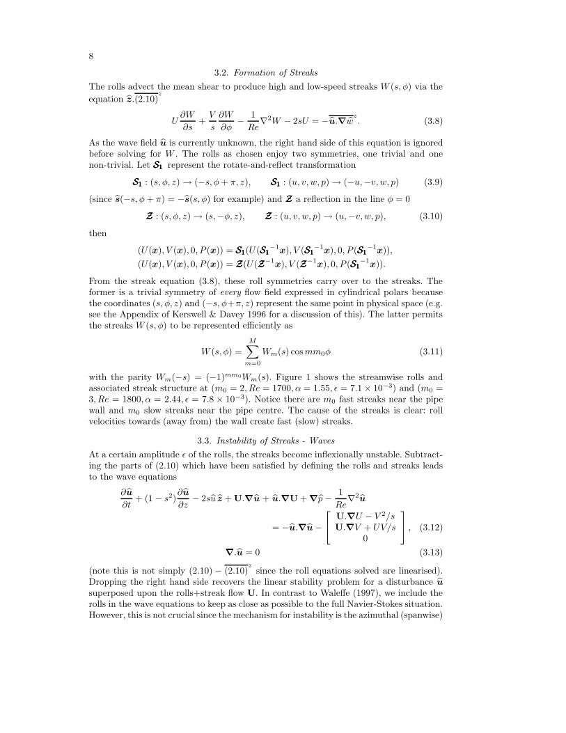
3.2. Formation of Streaks

The rolls advect the mean shear to produce high and low-speed streaks W (s, φ) via the

equation z.(2.10)z

U∂W

∂s+

V

s

∂W

∂φ−

1

Re∇2W − 2sU = −u.∇w

z. (3.8)

As the wave field u is currently unknown, the right hand side of this equation is ignoredbefore solving for W . The rolls as chosen enjoy two symmetries, one trivial and onenon-trivial. Let S1S1S1 represent the rotate-and-reflect transformation

S1S1S1 : (s, φ, z) → (−s, φ + π, z), S1S1S1 : (u, v, w, p) → (−u,−v, w, p) (3.9)

(since s(−s, φ + π) = −s(s, φ) for example) and ZZZ a reflection in the line φ = 0

ZZZ : (s, φ, z) → (s,−φ, z), ZZZ : (u, v, w, p) → (u,−v, w, p), (3.10)

then

(U(x), V (x), 0, P (x)) = S1S1S1(U(S1S1S1−1

x), V (S1S1S1−1

x), 0, P (S1S1S1−1

x)),

(U(x), V (x), 0, P (x)) = ZZZ(U(ZZZ−1x), V (ZZZ−1

x), 0, P (S1S1S1−1

x)).

From the streak equation (3.8), these roll symmetries carry over to the streaks. Theformer is a trivial symmetry of every flow field expressed in cylindrical polars becausethe coordinates (s, φ, z) and (−s, φ+π, z) represent the same point in physical space (e.g.see the Appendix of Kerswell & Davey 1996 for a discussion of this). The latter permitsthe streaks W (s, φ) to be represented efficiently as

W (s, φ) =

M∑

m=0

Wm(s) cos mm0φ (3.11)

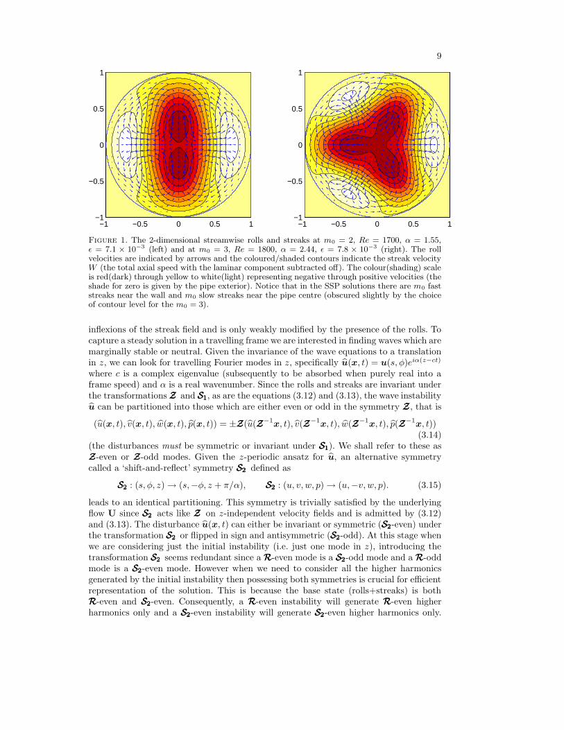
with the parity Wm(−s) = (−1)mm0Wm(s). Figure 1 shows the streamwise rolls andassociated streak structure at (m0 = 2, Re = 1700, α = 1.55, ε = 7.1 × 10−3) and (m0 =3, Re = 1800, α = 2.44, ε = 7.8 × 10−3). Notice there are m0 fast streaks near the pipewall and m0 slow streaks near the pipe centre. The cause of the streaks is clear: rollvelocities towards (away from) the wall create fast (slow) streaks.

3.3. Instability of Streaks - Waves

At a certain amplitude ε of the rolls, the streaks become inflexionally unstable. Subtract-ing the parts of (2.10) which have been satisfied by defining the rolls and streaks leadsto the wave equations

∂u

∂t+ (1 − s2)

∂u

∂z− 2su z + U.∇u + u.∇U + ∇p −

1

Re∇2u

= −u.∇u −

U.∇U − V 2/sU.∇V + UV/s

0

, (3.12)

∇.u = 0 (3.13)

(note this is not simply (2.10) − (2.10)z

since the roll equations solved are linearised).Dropping the right hand side recovers the linear stability problem for a disturbance u

superposed upon the rolls+streak flow U. In contrast to Waleffe (1997), we include therolls in the wave equations to keep as close as possible to the full Navier-Stokes situation.However, this is not crucial since the mechanism for instability is the azimuthal (spanwise)

9

−1 −0.5 0 0.5 1−1

−0.5

0

0.5

1

−1 −0.5 0 0.5 1−1

−0.5

0

0.5

1

Figure 1. The 2-dimensional streamwise rolls and streaks at m0 = 2, Re = 1700, α = 1.55,ε = 7.1 × 10−3 (left) and at m0 = 3, Re = 1800, α = 2.44, ε = 7.8 × 10−3 (right). The rollvelocities are indicated by arrows and the coloured/shaded contours indicate the streak velocityW (the total axial speed with the laminar component subtracted off). The colour(shading) scaleis red(dark) through yellow to white(light) representing negative through positive velocities (theshade for zero is given by the pipe exterior). Notice that in the SSP solutions there are m0 faststreaks near the wall and m0 slow streaks near the pipe centre (obscured slightly by the choiceof contour level for the m0 = 3).

inflexions of the streak field and is only weakly modified by the presence of the rolls. Tocapture a steady solution in a travelling frame we are interested in finding waves which aremarginally stable or neutral. Given the invariance of the wave equations to a translationin z, we can look for travelling Fourier modes in z, specifically u(x, t) = u(s, φ)eiα(z−ct)

where c is a complex eigenvalue (subsequently to be absorbed when purely real into aframe speed) and α is a real wavenumber. Since the rolls and streaks are invariant underthe transformations ZZZ and S1S1S1, as are the equations (3.12) and (3.13), the wave instabilityu can be partitioned into those which are either even or odd in the symmetry ZZZ , that is

(u(x, t), v(x, t), w(x, t), p(x, t)) = ±ZZZ(u(ZZZ−1x, t), v(ZZZ−1

x, t), w(ZZZ−1x, t), p(ZZZ−1

x, t))(3.14)

(the disturbances must be symmetric or invariant under S1S1S1). We shall refer to these asZZZ-even or ZZZ-odd modes. Given the z-periodic ansatz for u, an alternative symmetrycalled a ‘shift-and-reflect’ symmetry S2S2S2 defined as

S2S2S2 : (s, φ, z) → (s,−φ, z + π/α), S2S2S2 : (u, v, w, p) → (u,−v, w, p). (3.15)

leads to an identical partitioning. This symmetry is trivially satisfied by the underlyingflow U since S2S2S2 acts like ZZZ on z-independent velocity fields and is admitted by (3.12)and (3.13). The disturbance u(x, t) can either be invariant or symmetric (S2S2S2-even) underthe transformation S2S2S2 or flipped in sign and antisymmetric (S2S2S2-odd). At this stage whenwe are considering just the initial instability (i.e. just one mode in z), introducing thetransformation S2S2S2 seems redundant since a RRR-even mode is a S2S2S2-odd mode and a RRR-oddmode is a S2S2S2-even mode. However when we need to consider all the higher harmonicsgenerated by the initial instability then possessing both symmetries is crucial for efficientrepresentation of the solution. This is because the base state (rolls+streaks) is bothRRR-even and S2S2S2-even. Consequently, a RRR-even instability will generate RRR-even higherharmonics only and a S2S2S2-even instability will generate S2S2S2-even higher harmonics only.

10

This means that we can capture the full nonlinear solution emerging from a RRR-evenbifurcation within the space of RRR-even flows and the full nonlinear solution emergingfrom a RRR-odd bifurcation (i.e. a S2S2S2-even bifurcation) within the space of S2S2S2-even flows.This realisation is crucial for achieving the required levels of truncation within givencomputational constraints.

One final remark is due regarding the m0-fold periodicity in φ of the rolls+streaks.There will be fundamental disturbances possessing the same periodicity and non funda-

mental disturbances which take the form u(s, φ, z) = v(s, φ, z)eimφ where 0 < m < m0 isan integer and v is m0-fold periodic. In this work, the only non-fundamental disturbancesconsidered will be the simplest subharmonic disturbances where m = m0/2 which onlyexist if m0 is even. These will be RRRm0/2−waves. In summary, we can use the followingrepresentations of u to capture the main forms of instability. Fundamental modes are

uvwp

=

N−1∑

n=0

M∑

m=0

unmΘn(s; mm0) cosmm0φvnmΘn(s; mm0) sin mm0φwnmΦn(s; mm0) cosmm0φpnmΨn(s; mm0) cosmm0φ

eiα(z−ct) ZZZ − even (3.16)

uvwp

=

N−1∑

n=0

M∑

m=0

unmΘn(s; mm0) sin mm0φvnmΘn(s; mm0) cosmm0φwnmΦn(s; mm0) sinmm0φpnmΨn(s; mm0) sin mm0φ

eiα(z−ct) S2S2S2 − even (3.17)

and, if m0 is even, the subharmonic modes are

uvwp

=

N−1∑

n=0

M−1∑

m=0

unmΘn(s; (m + 12 )m0) cos[(m + 1

2 )m0φ]vnmΘn(s; (m + 1

2 )m0) sin[(m + 12 )m0φ]

wnmΦn(s; (m + 12 )m0) cos[(m + 1

2 )m0φ]pnmΨn(s; (m + 1

2 )m0) cos[(m + 12 )m0φ]

eiα(z−ct) ZZZ − even

(3.18)

uvwp

=

N−1∑

n=0

M−1∑

m=0

unmΘn(s; (m + 12 )m0) sin[(m + 1

2 )m0φ]vnmΘn(s; (m + 1

2 )m0) cos[(m + 12 )m0φ]

wnmΦn(s; (m + 12 )m0) sin[(m + 1

2 )m0φ]pnmΨn(s; (m + 1

2 )m0) sin[(m + 12 )m0φ]

eiα(z−ct) S2S2S2 − even

(3.19)

Here

Ψn(s; i) :=

{T2n+1(s) i odd,T2n(s) i even,

Θn(s; i) :=

{T2n+2(s) − T2n(s) i odd,T2n+3(s) − T2n+1(s) i even,

(3.20)

Φn(s; i) :=

{T2n+3(s) − T2n+1(s) i odd,T2n+2(s) − T2n(s) i even

(3.21)

where Tn(s) := cos(n cos−1 s) is the nth Chebyshev polynomial so that the boundaryconditions are built into the spectral functions. In this paper, we confine our attentionsolely to fundamental and subharmonic S2S2S2-even solutions (waves derived from wave in-stabilities of form (3.17) and (3.19)). Preliminary calculations indicated that these werethe first to appear for the chosen rolls. Future work will explore the ZZZ−even solutions.

Figure 2 shows typical streak instability profiles over wavenumber α for m0 = 2 and3. If the rolls are weaker than a threshold there is no streak instability. Beyond this,there are two neutral waves with the one at higher wavenumber giving by far the betterfeedback.

11

0 1 2 3 4−0.08

−0.07

−0.06

−0.05

−0.04

−0.03

−0.02

−0.01

0

0.01

0.02

α

α c i

0 1 2 3 4−0.12

−0.1

−0.08

−0.06

−0.04

−0.02

0

0.02

0.04

α

α c i

Figure 2. Streak instability growth rates αci (where ci is the imaginary part of c) as a functionof α and the roll amplitude ε. Left plot is for m0 = 2, Re = 1700 and roll amplitude ε = 0.009188(upper blue dashed), ε = 0.00711 (middle black solid) and ε = 0.005011 (lower red dash-dot).The vertical dotted line indicates the neutral wave mode at α = 1.55. The right plot is form0 = 3, Re = 1800 and roll amplitude ε = 0.00938 (upper blue dashed), ε = 0.0078 (middleblack solid) and ε = 0.00625 (lower red dash-dot). The vertical dotted line indicates the neutralwave mode at α = 2.44.

3.4. Nonlinear Feedback on the Rolls

As already mentioned, the crucial link in the SSP cycle is the nonlinear feedback ofthe waves onto the rolls. To assess this, the roll component of the form (U

′

(s) cos m0φ,V

′

(s) sin m0φ, 0) which would be induced by the waves u (through the right hand sidesof (3.3) and (3.4)) is calculated. The key issue is to establish whether the shape of theseinduced rolls matches that of the imposed rolls already in place (as given by (3.6)). Ifthere is significant overlap of structure then finite amplitude versions of these wavescan be expected to sustain the rolls against secular viscous decay. The amplitude of thewaves, which formally completes the ‘SSP’ approximate solution, is presumed set by thisprecise balancing and as is result is typically O(

√ε/Re).

To examine the feedback of a wave instability, we compare the radial velocity U′

(s)of the induced rolls with that of the imposed rolls. Applying s.∇×∇× to the equation

12

0 0.1 0.2 0.3 0.4 0.5 0.6 0.7 0.8 0.9 1−0.2

0

0.2

0.4

0.6

0.8

1

1.2

s

U

0 0.1 0.2 0.3 0.4 0.5 0.6 0.7 0.8 0.9 1−0.2

0

0.2

0.4

0.6

0.8

1

1.2

s

U

Figure 3. Plots showing good feedback. The radial velocity component of the imposed rolls is

plotted with the induced radial velocity component U′

(s) as calculated from (3.22) and nor-

malised appropriately. The top plot shows U′

(s) at Re = 1700 (red dash) and Re = 2100 (blackdot-dash) corresponding to the first S2S2S2-symmetric wave instability compared with the radialcomponent of the original rolls (blue solid) for m0 = 2 (α = 1.55). The bottom plot shows

U′

(s) at Re = 1800 (red dash) and Re = 2200 (black dot-dash) corresponding to the firstS2S2S2-symmetric wave instability compared with the radial component of the original rolls (bluesolid) for m0 = 3 (α = 2.44).

pair (3.3)-(3.4) leads to a single equation for the radial roll velocity

1

Re

(∇2 +

2

s

∂

∂s+

1

s2

)2

U = s.∇×∇×(u.∇uz) (3.22)

where the nonlinear roll terms are ignored due to their small amplitude. Only the pro-jection of the right hand side onto cosm0φ is used when inverting the linear operator tocalculate U

′

(s). A successful match (to be interpreted as significant overlap of profiles asfor example displayed in figure 3) indicates that the imposed streamwise rolls of ampli-tude ε, the associated streaks and the wave disturbance of some small amplitude set byroll energetic considerations constitutes a ‘SSP’ solution. The importance of such a ‘so-lution’ is that it gives an approximate location in parameter space in which to search foran exact travelling wave solution using the smooth continuation approach described inthe following section. In particular, information carried over to that analysis is the formof the initial rolls, their amplitude ε, the Reynolds number and the axial wavenumber

13

α for the wave instability. In practice, a subcritical bifurcation is always found close tothat predicted by the SSP analysis. However, there is no guarantee that this new solu-tion branch can be continued back to the zero-forcing situation. Typically, this can beengineered by increasing Re as will be discussed below. Figure 3 shows typical feedbackswhich were considered good enough to launch a more in depth search for a travellingwave solution via techniques described below.

4. Exact Solutions via Smooth Continuation

The key idea to convert the approximate analysis of the SSP to a more formal continu-ation setting is to add a body forcing to the Navier-Stokes equations (Waleffe 1998). Thisbody force is designed to initially maintain the streamwise rolls considered in the SSPanalysis against viscous decay in the absence of any other flow structures. Since theserolls were simply the least decaying eigenmodes of the linearised Stokesian operator (asgiven in (3.3) and (3.4)), the forcing function mirrors their structure. Specifically, thenew roll equations are

∂tU + Ps −1

Res.∇2U + s.(U.∇U) = fs(s, φ) − s.(u.∇u

z), (4.1)

∂tV +1

sPφ −

1

Reφ.∇2U + φ.(U.∇U) = fφ(s, φ) − φ.(u.∇u

z) (4.2)

where

fs(s, φ) := 2A[Jm0+1(λs) + Jm0−1(λs) − Jm0−1(λ)sm0−1] cosm0φ,

fφ(s, φ) := 2A[Jm0+1(λs) − Jm0−1(λs) + Jm0−1(λ)sm0−1] sinm0φ (4.3)

and A measures the forcing amplitude. Since the streamwise roll amplitude ε has been de-fined as the maximum value of the radial velocity component, then ignoring the nonlinearroll term (that is assuming ε � 1), the forced rolls have amplitude

ε =2ARe

λ2× max

s∈[0,1][Jm0+1(λs) + Jm0−1(λs) − Jm0−1(λ)sm0−1] (4.4)

If the forcing A goes beyond a threshold amplitude, a symmetry-breaking, 3-dimensionalstreak instability will occur as predicted by the SSP analysis near the appropriate stream-wise wavenumber α. The fact that this instability is known to have positive feedback onthe rolls makes it very likely (but not certain) that this bifurcation will be subcritical.(Considering the feedback onto the rolls only captures one half of the weakly nonlin-ear processes near the bifurcation since the excitation of the second harmonic is ignored.However, in our experience in this problem the former physics always dominates the latterand so finding positive feedback invariably implies subcriticality of the wave bifurcation.)Given this subcriticality, following the new solution branch corresponds to decreasing theforcing amplitude as the wave increasingly takes over the role of maintaining the rolls.In other words, as the wave amplitude grows along the solution branch, the two compo-nents of u.∇u

ztake over the role of (fs, fφ) in (4.1) and (4.2) of sustaining the rolls.

Ideally, the forcing amplitude can be reduced to zero at which point a fully nonlineartravelling solution to the physical pipe flow problem has been achieved. The SSP analysismerely isolates excellent candidates for continuation: it can say nothing about whetherthe continuation will ultimately cross the A = 0 axis. As way of illustration, it is possi-ble to construct SSP solutions down to Re ≈ 500 whereas the travelling waves are onlyfound to exist for Re ≥ 1600. What happens if the Re is too low is the solution branchreaches a minimum positive A before bending back to move towards increasing values of

14

A. However, continuing the branch to higher Re invariably moves this minimum throughthe A = 0 axis with the one notable exception of the fundamental S2S2S2−even m0 = 1 case.No travelling solution of this type was found to cross the A = 0 axis below Re = 6000despite starting with an SSP solution exhibiting excellent feedback (Faisst & Eckhardt(2003) also report a similar failure to find this mode).

4.1. Numerical Formulation

The problem, (2.10) (with body force f = fs(s, φ)s + fφ(s, φ)φ added) & (2.11), wassolved as stated - 3 momentum + 1 continuity equations - in terms of the primitivevariables (u, v, w, p) rather than any reduced representation of the velocity field such asa poloidal-toroidal decomposition. Experience indicates that this provides the best nu-merically conditioned formulation since spatial derivatives are kept at their lowest order.The governing equations were imposed by collocation over s and Galerkin projectionover φ and z. The axis of the pipe can cause numerical problems unless specific effortsare made to desensitize the code to this artificial singularity. This was achieved hereby exploiting the representation degeneracy of cylindrical polar coordinates in whichthe points (−s, φ ± π, z) and (s, φ, z) are exactly equivalent. This means that each ve-locity component and scalar pressure function has a definite parity in s determined bywhether its corresponding azimuthal wavenumber m is even or odd (see the appendixof Kerswell & Davey 1996). Building the appropriate radial parity into the spectralrepresentation of each field variable not only saves on storage but automatically instilsthe correct limiting behaviour near the axis. Computationally, we consider the domain{−1 ≤ s ≤ 1, 0 ≤ φ < π } rather than viewing the interior of the pipe as the region{ 0 ≤ s ≤ 1, −π ≤ φ < π }. The solution in −1 ≤ s < 0 can be constructed from thatin 0 < s ≤ 1 through the known symmetries and so we need only collocate the equa-tions over the positive zeros of T2N (s) and impose boundary conditions at s = 1. Mostimportantly, this means that the collocation points are at their sparsest near the axis -O(1/2N) spacing - and at their densest - O(1/4N 2) spacing - near the sidewall whereboundary layers typically need to be resolved.

Two types of travelling wave solutions were sought: fundamental S2S2S2-even solutions ofthe form

uvwp

=

N−1∑

n=0

M∑

m=0

{ L∑

l=1, l odd

unmlΘn(s; mm0) sinmm0φvnmlΘn(s; mm0) cosmm0φwnmlΦn(s; mm0) sin mm0φpnmlΨn(s; mm0) sin mm0φ

eiαl(z−ct)

+

L∑

l=0, l even

unmlΘn(s; mm0) cosmm0φvnmlΘn(s; mm0) sin mm0φwnmlΦn(s; mm0) cosmm0φpnmlΨn(s; mm0) cosmm0φ

eiαl(z−ct)

}+ c.c.

and, if m0 is even, subharmonic S2S2S2-even solutions of the form

uvwp

=

N−1∑

n=0

{ 2M∑

m=0, m even

L∑

l=0, l even

unmlΘn(s; 12mm0) cos 1

2mm0φvnmlΘn(s; 1

2mm0) sin 12mm0φ

wnmlΦn(s; 12mm0) cos 1

2mm0φpnmlΨn(s; 1

2mm0) cos 12mm0φ

eiαl(z−ct)

+

2M−1∑

m=1, m odd

L∑

l=1, l odd

unmlΘn(s; 12mm0) sin 1

2mm0φvnmlΘn(s; 1

2mm0) cos 12mm0φ

wnmlΦn(s; 12mm0) sin 1

2mm0φpnmlΨn(s; 1

2mm0) sin 12mm0φ

eiαl(z−ct)

}+ c.c.

15

where α is the primary axial wavenumber. As before, the appropriate boundary conditionsare built directly into the spectral expansion functions (see (3.20) and (3.21)). For agiven truncation (M, N, L), there were 2N(4ML + 4M + 4L + 1) real coefficients to bedetermined for the fundamental solution and 2N(4ML+4M +2L±1) in the subharmoniccase (+/− corresponding to L even/odd). One further equation,

=m

{N−1∑

n=0

un−11Θn(0.1;−m0)

}= 0, (4.5)

was imposed to eliminate the phase degeneracy of the travelling wave and served todetermine the wave speed c. The resultant nonlinear algebraic system,

FFF(ulmn, vlmn, wlmn, plmn, c ; Re, A, α) = 0, (4.6)

was solved given a nearby starting solution using the PITCON package developed byRheinboldt and Burkardt (1983a,b) which is a robust branch-following program basedupon Newton-Raphson iteration. Typically up to 16, 000 degrees of freedom were used(requiring sub-2GB storage) but occasionally up to 20, 000 degrees of freedom (3GBstorage) were used to confirm convergence.

5. Results

5.1. Searching for Travelling Waves

The search for SSP solutions proceeded by first choosing m0, selecting the least decayingstreamwise rolls and then adjusting their amplitude ε until the streak field became un-stable at a given Reynolds number Re and axial wavelength α. The feedback associatedwith this wave instability was then checked for compatibility with the initial rolls. If thematch was very good (i.e. there was a strong positive correlation between the structureof the induced and imposed rolls), this set of parameters (m0, λm0 1, ε, Re, α) was usedas a starting point in parameter space to initiate the smooth continuation procedure of§4. If instead the match was poor, indicated by a negative correlation between the radialvelocity components of induced and imposed rolls, a number of corrective strategies couldbe employed: vary Re, increase ε further and select a new instability or adjust α. By farthe most effective of these was to vary α to which the feedback seemed very sensitive.

Figures 4 and 5 show the result of carrying out this procedure for the SSP solutionsat (m0, α, Re) = (2, 1.55, 2100) and (m0, α, Re) = (3, 2.44, 1800) discussed above. Themeasure

3D amp :=

√√√√N−1∑

n=0

|un11|2 + |vn11|2 + |wn11|2 (5.1)

plotted on the (left) y-axis is used to indicate the degree of 3-dimensionality of the solu-tion. In each figure, the two curves shown represent the data from one run of the branchtracing process at a representative truncation level. All the individual convergences ofthe root-finding algorithm are displayed (joined by straight lines to guide the eye) toindicate the relative ease (measured in terms of number of steps taken) at which thesolution branch can be continued back the A = 0 axis. The jaggedness seen in the plotsarises through any of three different effects. Firstly, and dominantly, there is the strobing

16

Figure 4. The continuation curve for m0 = 2, α = 1.55 at Re = 2100 (truncation (8,25,5)). Thesolid (blue) line shows how the forcing amplitude A can be decreased from Acrit = 7.44 × 10−5

as a 3D amplitude measure increases (note the parabolic head indicative of a subcritical bi-furcation). There are two crossings of the pipe flow limit (A = 0) representing an upper andlower branch of travelling wave solutions. The dashed (green) line shows that the lower branchhas faster travelling waves than the upper branch. The dots show specific convergences of thepath-finding procedure indicating how easy or difficult the solution is to follow.

of the true smooth curve since only a finite number of solutions are shown joined bystraight lines. Secondly, the projection of a smooth curve in higher dimensions onto theA−3D amp plane can cause apparent jerkiness and thirdly, the use of an insufficienttruncation level can lead to sharp changes in the solution curve (the last effect is consid-ered in more detail later). For the truncation level chosen, the path back to the unforcedpipe flow situation (A = 0) in figure 4 (m0 = 2) is direct and there are the expected2 crossings corresponding to an upper and lower branch. Figure 5 (m0 = 3), however,shows an indirect connection back to the A = 0 axis, hinting at the possibility of moreconvoluted behaviour. This is confirmed in figure 6 by considering the same SSP solution(m0, α) = (3, 2.44) but further away from the saddle node bifurcation at Re = 2200.After the initial smooth path back, the solution curve knits itself around the A = 0 axiscrossing 6 times implying 3 separate upper and lower branch pairings. If these 6 solutions(along with the 2 for m0 = 2) are used as starting points for branch continuation, thecurves traced out are as in figure 7. This confirms that there is one solution branch form0 = 2 at truncation (M, N, L) = (8, 25, 5) and α = 1.55 (corroborated by higher trun-cations) and three separate branches for m0 = 3 at (M, N, L) = (8, 24, 5) and α = 2.44

17

Figure 5. The continuation curve for m0 = 3, α = 2.44 at Re = 1800 (Acrit = 1.7962 × 10−4

as opposed to Acrit = 1.75 × 10−4 predicted from the SSP analysis: truncation (8,24,5)). Againthere are two crossings of the pipe flow limit (A = 0) representing an upper and lower branchof travelling wave solutions.

(partially confirmed by higher truncations; see below). The m0 = 3 branch which reachesthe lowest Re value of 1617 is the only branch existing at Re = 1800 (see figure 5) andachieves the smallest Rem = 1251 (at Re = 1631).

The most notable difference in the structure of the multiple m0 = 3 solutions is thenumber of fast streaks near the wall. Figure 8 shows streamwise-averaged plots of the totalcross-stream velocity, v⊥ := us+ vφ, and the surplus streamwise speed w for solutions a-f as marked on figures 6 and 7. Streamwise-averaging the velocity field brings into sharpfocus the direct link between the streaks and the cross-stream flow which is arrangedinto a series of coherent rolls. Plotting contours of w emphasizes the differences in theaxial velocity of the travelling wave from that of the laminar solution which correspondsto the same applied pressure gradient or equivalently the same Re. From figure 6 (andthe dashed A − c curve), the first crossing of A = 0 corresponds to solution a which hasm0 = 3 fast streaks near the wall. Not unexpectedly, this is very similar to the startingSSP roll+streak ansatz at the initial bifurcation point (A, 3D amp) = (Acrit, 0) displayed

18

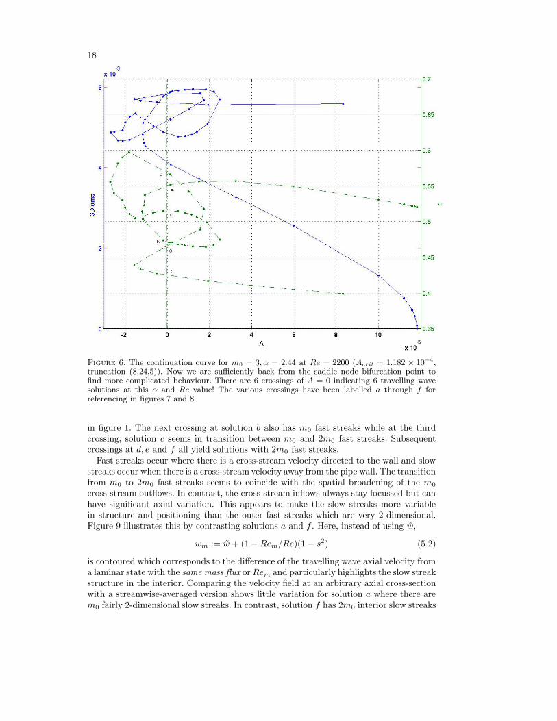
Figure 6. The continuation curve for m0 = 3, α = 2.44 at Re = 2200 (Acrit = 1.182 × 10−4,truncation (8,24,5)). Now we are sufficiently back from the saddle node bifurcation point tofind more complicated behaviour. There are 6 crossings of A = 0 indicating 6 travelling wavesolutions at this α and Re value! The various crossings have been labelled a through f forreferencing in figures 7 and 8.

in figure 1. The next crossing at solution b also has m0 fast streaks while at the thirdcrossing, solution c seems in transition between m0 and 2m0 fast streaks. Subsequentcrossings at d, e and f all yield solutions with 2m0 fast streaks.

Fast streaks occur where there is a cross-stream velocity directed to the wall and slowstreaks occur when there is a cross-stream velocity away from the pipe wall. The transitionfrom m0 to 2m0 fast streaks seems to coincide with the spatial broadening of the m0

cross-stream outflows. In contrast, the cross-stream inflows always stay focussed but canhave significant axial variation. This appears to make the slow streaks more variablein structure and positioning than the outer fast streaks which are very 2-dimensional.Figure 9 illustrates this by contrasting solutions a and f . Here, instead of using w,

wm := w + (1 − Rem/Re)(1 − s2) (5.2)

is contoured which corresponds to the difference of the travelling wave axial velocity froma laminar state with the same mass flux or Rem and particularly highlights the slow streakstructure in the interior. Comparing the velocity field at an arbitrary axial cross-sectionwith a streamwise-averaged version shows little variation for solution a where there arem0 fairly 2-dimensional slow streaks. In contrast, solution f has 2m0 interior slow streaks

19

1600 1700 1800 1900 2000 2100 22000.4

0.5

0.6

0.7

Re

c

a

b

c

d

e

f

Figure 7. The travelling wave solution curves traced out by taking the solutions found from thecontinuations reported in figures 4 (truncation (8, 25, 5)), 5 and 6 (both at truncation (8, 24, 5)).The m0 = 2 (blue) dash-dot curve (α = 1.55)is one pair of upper and lower branches corre-sponding to a saddle node bifurcation at lower Re. In contrast there are multiple m0 = 3 (red)curves (solid and dashed) at α = 2.44. The labelling (a to f) used in figure 6 is reproduced hereto indicate the correspondence between the crossings and the various branches. Note that theapparent crossings of the m0 = 3 curves are due to projection onto a plane and not bifurcations.

with significant 3-dimensional variation so that their streamwise average becomes almostfeatureless in the interior.

All these solutions except for the ‘transitional’ solution c can be confirmed using in-creased truncation levels. Figure 10 shows the results of following the branches using avariety of larger truncations. (A branch section is inferred to exist and drawn with asolid or dashed line if a variety of truncations traced it out successfully.) The presenceof multiple branches on this slice (α = 2.44) of the m0 = 3 solution surface is confirmedalthough there appear two branches (see the (9, 26, 6) results in figure 10) rather than thethree suggested in figure 7 by the lower truncation of (8, 24, 5) (which still represents over10,000 degrees of freedom). The structure of the flow solutions on the branches whichextend to higher Rem (> 2600) closely resembles the corresponding solution structureillustrated in figure 8. For example, on the lowest branch which passes through solutionf , the travelling wave at Rem = 2600 has 2m0 fast streaks equispaced around the pipeperimeter just like f . The one notable exception to this observation is provided by thebranch corresponding to solution e. Here there are 2m0 fast streaks as for solution e but

20

−1 0 1−1

−0.5

0

0.5

1a

−1 0 1−1

−0.5

0

0.5

1b

−1 0 1−1

−0.5

0

0.5

1c

−1 0 1−1

−0.5

0

0.5

1f

−1 0 1−1

−0.5

0

0.5

1d

−1 0 1−1

−0.5

0

0.5

1e

Figure 8. Streamwise-averaged plots of the various solutions labelled in figure 6 to show theirdifferent streak structure. The arrows indicate the streamwise-averaged cross-stream velocitiesv⊥

z (larger arrows corresponding to larger speeds) and the coloring (shading) represents the

streamwise-averaged axial velocity differential, wz

(red,dark = most negative and white(light)most positive; the colour/shading of the area exterior to the pipe represents zero). Solutionsare arranged in branch pairings - a and b, c and f , and d and e - and so that the respectiveupper (lower) branch solution (referring to figure 7) is on the left (right). Since all solutionscorrespond to Re = 2200 the contour levels are kept constant across the figures (from -0.5to 0.5 in steps of 0.031) to highlight their relative magnitude of w

z

. Quantitatively, (min(wz

),

max(wz

),max(|v⊥|z

)) =(-0.31,0.057,0.011) for a, (-0.33,0.047,0.018) for b, (-0.25,0.037,0.015) forc, (-0.28,0.065,0.013) for d, (-0.39.0.068.0.017) for e and (-0.40,0.059,0.020) for f (a speed of 1corresponds to the centreline speed of the laminar solution at a Reynolds number of Re).

they not equally spaced around the pipe perimeter, appearing ready to merge in pairs.Figure 11 shows both w and w + (1 − Rem/Re)(1 − s2) contoured for this solution atone cross-section of the pipe. The constant mass plot on the right shows the presence ofm0 = 3 dominant slow streaks in the interior indicating that there is no simple connec-

21

−1 −0.5 0 0.5 1−1

−0.5

0

0.5

1a α* z=0

−1 −0.5 0 0.5 1−1

−0.5

0

0.5

1a z−averaged

−1 −0.5 0 0.5 1−1

−0.5

0

0.5

1f α* z=0

−1 −0.5 0 0.5 1−1

−0.5

0

0.5

1f z−averaged

Figure 9. Velocity fields for the RRR3 solutions a (upper) and f (lower) of figure 7. The left plotsare show contour plots of wm = w + (1 − Rem/Re)(1 − s2) and arrow plots of the cross-streamvelocity at a given z-station along the pipe (arbitrarily chosen as z = 0). The right plots are thez-average of wm and the cross-stream velocity along the pipe. There are 10 contour levels in theupper plots ranging from -0.18 to 0.14 and 10 contour levels in the lower plots ranging from -0.14to 0.16. These plots illustrate how the fast streaks near the wall are effectively 2-dimensionalwhereas the slow interior streaks can have an appreciable 3-dimensional element. The slowstreaks only oscillate slightly around in space in the upper solution a as evidenced in the fairlyclose match with the streamwise averaged field. In contrast, there is much more variation inthe interior of solution f where the streamwise-average looks featureless but a typical slice has6 well defined slow streaks. Subtracting off the equivalent laminar flow of the same mass fluxleads to clearer visualisation of the slower fluid velocities near the centre of the pipe: comparethese averaged plots with those of figure 8.

tion between the number of fast streaks and slow streaks (see also the RRR2 wave in figure12 below).

5.2. Travelling Wave Solutions

The objective once a travelling wave solution had been found was to map out the solutionsurface as much as was practical until

minRe,α

Rem(m0)

22

1200 1400 1600 1800 2000 2200 2400 2600 2800 3000 3200

0.3

0.35

0.4

0.45

0.5

0.55

0.6

0.65

Rem

c

a

b

c

d

e

f

Figure 10. An exploration of numerical convergence for the multiple solution branches for RRR3

revealed in figure 7. The solutions a-f at Re = 2200 are marked as in figure 7 but now overRem. A solid or dashed line indicates where a solution branch has been confirmed by differenttruncation levels (the dashed line corresponds to the dashed curve in figure 7). This showsthat the (8, 24, 5) solutions a, b, d, e and f are real (although e is poorly resolved) and that cis a numerical artefact. Notice that (9, 26, 6) indicates that there are 2 separate branches. Thetruncation levels (M, N, L) used are • (8, 24, 5), ∗ (8, 24, 6), � (8, 24, 7), � (8, 26, 5), × (9, 26, 6),4 (8, 28, 6), ◦ (9, 28, 5).

was found. Given the multiple solution branches already found for m0 = 3, this is adaunting numerical undertaking. As a result, we have contented ourselves here with get-ting onto a solution surface for each m0 value up to 6 using the SSP analysis to guideour starting point and then searching smoothly around on this for minRe,α Rem(m0). So,given this uncertainty of the solution surface topology, we can say only that RRRm0

−wavescertainly exist down to some value of Rem rather than the stronger (and preferable)statement that RRRm0

−waves only appear for Rem above some threshold value. To em-phasize this, figures 12 and 13 indicate that we have found 2m0-streak solutions form0 = 2, 3, 4 at the respective saddle node bifurcation but only m0-streak solutions form = 5, 6. Whether corresponding solutions of the other type exist at lower Rem remainsuncertain. Faisst & Eckhardt (2003) do report finding a 2m0-streak solution for m0 = 5but admit that it is not properly resolved.

23

−1 −0.5 0 0.5 1−1

−0.5

0

0.5

1

−1 −0.5 0 0.5 1−1

−0.5

0

0.5

1

Figure 11. The structure of a RRR3 travelling wave on the solution branch corresponding to e atα = 2.44, c = 0.456 and Rem = 3378 (see figure 10) at a given pipe cross section (truncation(9,26,6)). On the left, w is contoured (constant Re) whereas on the right, contours are drawnfor wm (constant Rem). In both plots, 12 contours are drawn between the maximum and min-imum values of w (-0.47,0.089) and wm (-0.17,0.19). The right hand plot shows the three slowstreaks near the pipe axis particularly well. As elsewhere, the shading(colour) outside the pipecorresponds to the 0 level.

−1 −0.5 0 0.5 1−1

−0.5

0

0.5

1

−1 −0.5 0 0.5 1−1

−0.5

0

0.5

1

Figure 12. RRR1 and RRR2 travelling waves at their saddle node bifurcation points andoptimal wavenumber. The arrows indicate the streamwise-averaged cross-stream velocities

v⊥z = u

zbs + vz bφ (larger arrows corresponding to larger speeds) and the coloring (shading)

represents the streamwise-averaged axial velocity differential wmz (red/dark = most negative

and white/light most positive; the colour/shading of the area exterior to the pipe representszero). Ten contours are drawn between the maximum and minimum values of wm

z as listed inTable 2. Streamwise-averaging highlights the structure of the waves most clearly.

Figure 14 hints at the complexity of the situation. Here two known RRR3 and RRR4 solutionsat Rem = 2000 were used as starting points to trace out their respective solution surfacecross-sections defined by Rem = 2000. The initial motivation for this was to assess the

24

−1 −0.5 0 0.5 1−1

−0.5

0

0.5

1

−1 −0.5 0 0.5 1−1

−0.5

0

0.5

1

−1 −0.5 0 0.5 1−1

−0.5

0

0.5

1

−1 −0.5 0 0.5 1−1

−0.5

0

0.5

1

Figure 13. RRRm0travelling waves for m0 = 3, 4, 5, 6 at their saddle node bifurcation points

and optimal wavenumber. The arrows indicate the streamwise-averaged cross-stream velocities

v⊥z = u

zbs + vz bφ (larger arrows corresponding to larger speeds) and the coloring (shading)

represents the streamwise-averaged axial velocity differential wmz (red/dark = most negative

and white/light most positive; the colour/shading of the area exterior to the pipe representszero). Ten contours are drawn between the maximum and minimum values of wm

z as listed inTable 2. Streamwise-averaging highlights the structure of the waves most clearly.

range of α and C = cW/W (the phase speed normalised by the average streamwise speed)over which the travelling waves exist at this experimentally relevant Rem. While this datacertainly emerges − 1.0 < α < 3.1 & 1.09 < C < 1.45 for RRR3 and 2.38 < α < 3.6 &1.06 < C < 1.26 for RRR4 − the more striking information revealed is how the two RRR3

solutions branches already found are smoothly connected and the discovery of two RRR4

solution branches at α = α∗4 = 3.23. The four crossings of the optimal wavenumber

α = 2.44 line by the RRR3 curve coincide with the branches shown in figure 10: startingfrom the highest C value and in descending order, the intersections are by the branchescorresponding to solutions d, a, e and f . Both loops of the RRR4 wave solutions have 2m0

streaks with the upper (in C) larger (and better converged) loop leading to a lowest Rem

value of 1647 (see Table 2 below).

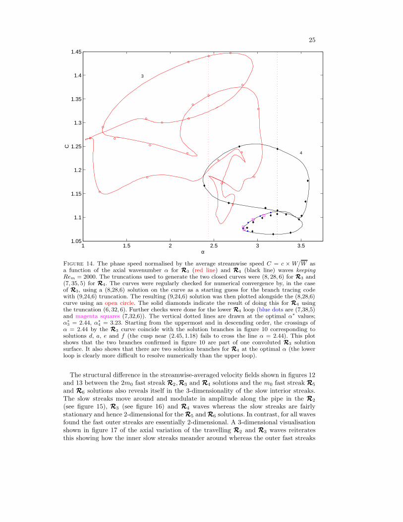
25

1 1.5 2 2.5 3 3.51.05

1.1

1.15

1.2

1.25

1.3

1.35

1.4

1.45

3

4

α

C

Figure 14. The phase speed normalised by the average streamwise speed C = c × W/W asa function of the axial wavenumber α for RRR3 (red line) and RRR4 (black line) waves keepingRem = 2000. The truncations used to generate the two closed curves were (8, 28, 6) for RRR3 and(7, 35, 5) for RRR4. The curves were regularly checked for numerical convergence by, in the caseof RRR3, using a (8,28,6) solution on the curve as a starting guess for the branch tracing codewith (9,24,6) truncation. The resulting (9,24,6) solution was then plotted alongside the (8,28,6)curve using an open circle. The solid diamonds indicate the result of doing this for RRR4 usingthe truncation (6, 32, 6). Further checks were done for the lower RRR4 loop (blue dots are (7,38,5)and magenta squares (7,32,6)). The vertical dotted lines are drawn at the optimal α∗ values;α∗

3 = 2.44, α∗4 = 3.23. Starting from the uppermost and in descending order, the crossings of

α = 2.44 by the RRR3 curve coincide with the solution branches in figure 10 corresponding tosolutions d, a, e and f (the cusp near (2.45, 1.18) fails to cross the line α = 2.44). This plotshows that the two branches confirmed in figure 10 are part of one convoluted RRR3 solutionsurface. It also shows that there are two solution branches for RRR4 at the optimal α (the lowerloop is clearly more difficult to resolve numerically than the upper loop).

The structural difference in the streamwise-averaged velocity fields shown in figures 12and 13 between the 2m0 fast streak RRR2,RRR3 and RRR4 solutions and the m0 fast streak RRR5

and RRR6 solutions also reveals itself in the 3-dimensionality of the slow interior streaks.The slow streaks move around and modulate in amplitude along the pipe in the RRR2

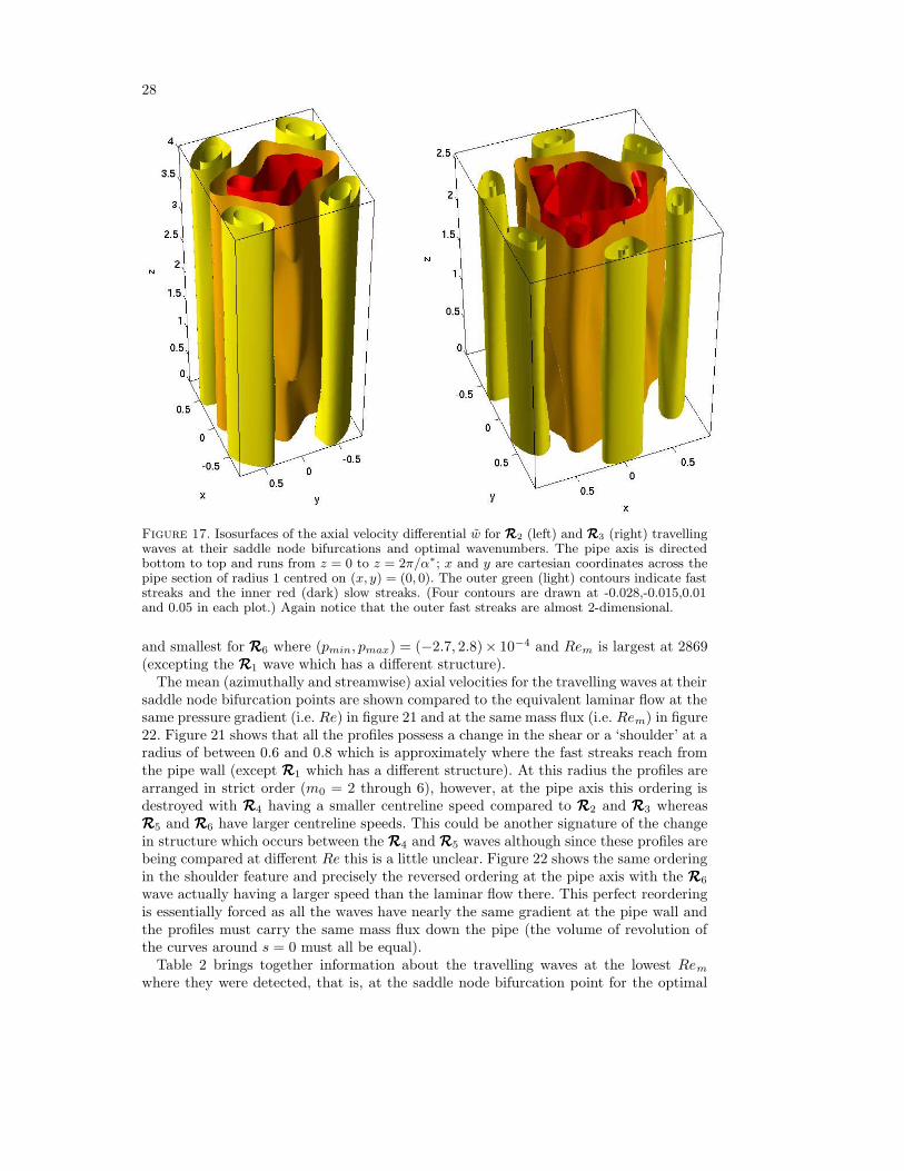
(see figure 15), RRR3 (see figure 16) and RRR4 waves whereas the slow streaks are fairlystationary and hence 2-dimensional for the RRR5 and RRR6 solutions. In contrast, for all wavesfound the fast outer streaks are essentially 2-dimensional. A 3-dimensional visualisationshown in figure 17 of the axial variation of the travelling RRR2 and RRR3 waves reiteratesthis showing how the inner slow streaks meander around whereas the outer fast streaks

26

−1 −0.5 0 0.5 1−1

−0.5

0

0.5

1 α* z=0

−1 −0.5 0 0.5 1−1

−0.5

0

0.5

1α* z=π/4

−1 −0.5 0 0.5 1−1

−0.5

0

0.5

1α* z=π/2

−1 −0.5 0 0.5 1−1

−0.5

0

0.5

1α* z=3π/4

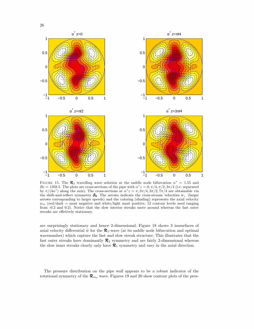
Figure 15. The RRR2 travelling wave solution at the saddle node bifurcation α∗ = 1.55 andRe = 1358.5. The plots are cross-sections of the pipe with α∗z = 0, π/4, π/2, 3π/4 (i.e. separatedby π/(4α∗) along the axis). The cross-sections at α∗z = π, 5π/4, 3π/2, 7π/4 are obtainable viathe shift-and-reflect symmetry S2S2S2. The arrows indicate the cross-stream velocities v⊥ (largerarrows corresponding to larger speeds) and the coloring (shading) represents the axial velocitywm (red/dark = most negative and white/light most positive, 12 contour levels used rangingfrom -0.2 and 0.2). Notice that the slow interior streaks move around whereas the fast outerstreaks are effetively stationary.

are surprisingly stationary and hence 2-dimensional. Figure 18 shows 3 isosurfaces ofaxial velocity differential w for the RRR1-wave (at its saddle node bifurcation and optimalwavenumber) which capture the fast and slow streak structure. This illustrates that thefast outer streaks have dominantly RRR2 symmetry and are fairly 2-dimensional whereasthe slow inner streaks clearly only have RRR1 symmetry and vary in the axial direction.

The pressure distribution on the pipe wall appears to be a robust indicator of therotational symmetry of the RRRm0

wave. Figures 19 and 20 show contour plots of the pres-

27

−1 −0.5 0 0.5 1−1

−0.5

0

0.5

1 α* z=0

−1 −0.5 0 0.5 1−1

−0.5

0

0.5

1α* z=π/4

−1 −0.5 0 0.5 1−1

−0.5

0

0.5

1α* z=π/2

−1 −0.5 0 0.5 1−1

−0.5

0

0.5

1α* z=3π/4

Figure 16. The RRR3 travelling wave solution at the saddle node bifurcation α∗ = 2.44 andRe = 1250.9. The plots are cross-sections of the pipe with α∗z = 0, π/4, π/2, 3π/4 (i.e. separatedby π/(4α∗) along the axis). The cross-sections at α∗z = π, 5π/4, 3π/2, 7π/4 are obtainable viathe shift-and-reflect symmetry S2S2S2. The arrows indicate the cross-stream velocities (larger arrowscorresponding to larger speeds) and the coloring (shading) represents the axial velocity (red,dark= most negative and white(light) most positive, 12 contour levels using ranging from -0.15 to0.15). Notice that the slow interior streaks move around whereas the fast outer streaks are fairlystationary.

sure distribution on the pipe wall for the RRRm0solutions at their respective saddle node

bifurcations. The number of pressure peaks around a pipe circumference is exactly m0

regardless of whether there are m0 or 2m0 fast streaks. This is because the pressure fieldis decoupled from the streamwise-independent axial flow structures. As way of confir-mation, the pressure fields associated with the various m0 = 3 solutions a, b, d, e and fproduce exactly similar plots to that shown in figure 19 albeit the individual cells varyin exact shape somewhat. Furthermore, the RRR1 wave has two fast streaks but only onepressure maximum around the boundary at a given station z along the pipe. The rangeof the pressure values at the wall (in non-dimensional units of ρW 2) is largest for RRR3

at (pmin, pmax) = (−7.9, 7.8) × 10−4 corresponding to the lowest Rem value of 1251,

28

Figure 17. Isosurfaces of the axial velocity differential w for RRR2 (left) and RRR3 (right) travellingwaves at their saddle node bifurcations and optimal wavenumbers. The pipe axis is directedbottom to top and runs from z = 0 to z = 2π/α∗; x and y are cartesian coordinates across thepipe section of radius 1 centred on (x, y) = (0, 0). The outer green (light) contours indicate faststreaks and the inner red (dark) slow streaks. (Four contours are drawn at -0.028,-0.015,0.01and 0.05 in each plot.) Again notice that the outer fast streaks are almost 2-dimensional.

and smallest for RRR6 where (pmin, pmax) = (−2.7, 2.8)× 10−4 and Rem is largest at 2869(excepting the RRR1 wave which has a different structure).

The mean (azimuthally and streamwise) axial velocities for the travelling waves at theirsaddle node bifurcation points are shown compared to the equivalent laminar flow at thesame pressure gradient (i.e. Re) in figure 21 and at the same mass flux (i.e. Rem) in figure22. Figure 21 shows that all the profiles possess a change in the shear or a ‘shoulder’ at aradius of between 0.6 and 0.8 which is approximately where the fast streaks reach fromthe pipe wall (except RRR1 which has a different structure). At this radius the profiles arearranged in strict order (m0 = 2 through 6), however, at the pipe axis this ordering isdestroyed with RRR4 having a smaller centreline speed compared to RRR2 and RRR3 whereasRRR5 and RRR6 have larger centreline speeds. This could be another signature of the changein structure which occurs between the RRR4 and RRR5 waves although since these profiles arebeing compared at different Re this is a little unclear. Figure 22 shows the same orderingin the shoulder feature and precisely the reversed ordering at the pipe axis with the RRR6

wave actually having a larger speed than the laminar flow there. This perfect reorderingis essentially forced as all the waves have nearly the same gradient at the pipe wall andthe profiles must carry the same mass flux down the pipe (the volume of revolution ofthe curves around s = 0 must all be equal).

Table 2 brings together information about the travelling waves at the lowest Rem

where they were detected, that is, at the saddle node bifurcation point for the optimal

29

Figure 18. Isosurfaces of axial velocity differential w for the RRR1-wave at its saddle node bifur-cation and optimal wavenumber. The pipe axis is directed bottom to top and runs from z = 0to z = 2π/α∗

1; x and y are cartesian coordinates across the pipe section of radius 1 centred on(x, y) = (0, 0). The outer green (light) contours at 0 and 0.1 indicate the 2 fast streaks whichare very close to the wall at (x, y) = (0,±1) and the inner red (darker) contour at -0.255 showsup the slow streaks. Only three contour levels have been chosen to illustrate that the fast outerstreaks have dominantly RRR2 symmetry but the slow inner streaks clearly only have RRR1.

wavenumber α∗. There appear a number of systematic trends as m0 increases. Firstly,the critical Rem value grows presumably because the fast streaks are pushed towards thepipe wall and hence suffer enhanced dissipation. The optimal wavenumber α∗ increases insympathy with the smaller streak scales generated near the wall. The waves also becomeslower and the mean velocity decreases. The structural differences in the waves are alsoapparent from the simple velocity measures shown too. RRR1-waves stand out by havingfast streak w velocities comparable to its slow streak w velocities whereas in all theother waves, the latter dominate the former. If, instead, wm is considered, the fast andslow streaks are essentially of equal magnitude for the modes except RRR1. The peak slow

30

0 2 4 60

1

2

3

4

φ

z

m0=1

0 2 4 60

1

2

3

4

φ

z

m0=2

0 2 4 60

1

2

3

4

φ

z

m0=3

0 2 4 60

1

2

3

4

φ

z

m0=4

Figure 19. The pressure field at the pipe wall s = 1 associated with the RRRm0travelling waves

at their minimum Rem values (and hence optimal α = α∗). For ease of comparison, the pressurefields are contoured over 0 ≤ φ ≤ 2π and 0 ≤ z ≤ 2π/α∗

2 where α∗2 = 1.55 is the smallest optimal

wavenumber over m0 = 1 to 6 and so corresponds to the longest wavelength. Equally-spacedcontours are drawn ranging from the pressure minimum pmin to the pressure maximum pmax (12drawn for m0 = 1, 2, 3 and 10 for m0 = 4) and dark(red) corresponds to negative values whereaslight(white) to positive values. (pmin, pmax) = (−3.0, 3.8) × 10−4 for RRR1, (−5.0, 4.6) × 10−4 forRRR2, (−7.9, 7.8) × 10−4 for RRR3 and (−6.2, 7.6) × 10−4 for RRR4.

streak w velocity is fairly uniform across all the fundamental waves but the 2m0-faststreak solutions (RRRm0

m0=2,3,4) have stronger cross-stream velocities than the m0 faststreak solutions (RRRm0

m0=5,6). In all cases, the streak velocities are typically an order ofmagnitude larger than the cross-stream velocities. The entries for RRR2 and RRR3 confirm andimprove the results quoted by Faisst & Eckhardt (2003) since much higher truncationlevels are used here.

Figure 23 shows the various travelling solution branches traced as far as they couldbe assured resolved by overlaying curves from different truncation runs. The systematictrend in the phase speed (decreasing as m0 increases) is particularly apparent as arethe respective positions of the critical Rem(m0). The fact that the subharmonic RRR1-wave curve flanks the fundamental RRR2 curve suggests that pursuing subharmonic andother forms of RRRm streak-instability based on a RRR2m roll + streak structure may alwaysproduce solutions with similar neighbouring curves to the fundamental RRR2m curve. The

31

0 pi/20

0.5

1

1.5

2

2.5

3

3.5

4

φ

z

m0=4

0 2pi/50

0.5

1

1.5

2

2.5

3

3.5

4

φ

z

m0=5

0 pi/30

0.5

1

1.5

2

2.5

3

3.5

4

φ

z

m0=6

Figure 20. The pressure field at the pipe wall s = 1 associated with the RRRm0(m0 = 4, 5, 6)

travelling waves at their minimum Rem values (and hence optimal α = α∗). As in figure 19,contours are drawn over 0 ≤ z ≤ 2π/α∗

2 but for clarity, φ is now restricted to [0, 2π/m0]. TheRRR4 pressure field is reproduced here for comparison purposes. As in figure 19, 12 contours aredrawn at equal intervals ranging from the minimum pressure pmin to the maximum pressurepmax: (pmin, pmax)= (−6.2, 7.6)× 10−4 for RRR4, (−3.2, 3.3)× 10−4 for RRR5 and (−2.7, 2.8)× 10−4

for RRR6.

dissipation rate associated with these RRRm0-waves is compared in figure 24 to the Hagen-

Poiseuille value and the experimental log-law parametrisation of post-transition flows.Interestingly, the dissipation rates associated with RRR2, RRR3 and RRR4 waves can exceed thelog-law value, although only the RRR3 and RRR4 branches manage this at post-transitionalRem. It is tempting to speculate that there may well be other RRR5 and RRR6 waves whichalso have such high friction factors yet to be found. An obvious strategy to explore thisis to repeat the solution tracing exercise reported in figure 14 since this was how thedissipative RRR4-wave branch was discovered. Unfortunately, however, it is no coincidencethat the travelling wave solutions with the largest friction factors are also the hardest toresolve numerically. The solution branches which have been numerically resolved throughto Rem = 3500 all have the same (weak) asymptotic friction behaviour as the laminarHagen-Poiseuille flow albeit with a larger numerical coefficient.

32

0 0.1 0.2 0.3 0.4 0.5 0.6 0.7 0.8 0.9 1−1

−0.8

−0.6

−0.4

−0.2

0

0.2

0.4

0.6

0.8

1

s

w

Figure 21. The mean axial velocity profile for the RRRm0(m0 = 1, ..., 6) travelling waves at

their saddle node points and (hence optimal wavenumbers). The profiles are compared to theequivalent laminar profile (dotted line) at the same applied pressure gradient (i.e. same Re).The axial velocity corresponding to RRR1 is the thick, cyan, dashed line, RRR2 is the thick, blue,dash-dot line, RRR3 is the thick, red, solid line, RRR4 is the thin, black, dashed line, RRR5 is the thick,magenta, dash-dot line and RRR6 is the thin, blue, solid line. Going from right to left along theradius s = 0.6, the curves correspond to the laminar state 1 − s2, RRR2, RRR1, RRR3, RRR4, RRR5 andfinally RRR6.

Figures 25, 26 and 27 indicate how the numerical values for Rem quoted in Table 2 aredecided upon. Identifying minα,ReRem(m0) is a painstaking task since the search is overa 2-d parameter space and the appropriate truncation level required for a given accuracyis unknown a priori. The strategy adopted was to use a moderately high truncationlevel to isolate the neighbourhood of the minimum before employing a suite of highertruncations to assess the likely accuracy given the inevitable hardware restrictions. Forexample, in the case of RRR3, the truncation (M, N, L) = (8, 24, 5) proves adequate tolocate α∗

3 (checked by truncations (9,25,6) and (10,24,5)). Then higher resolutions suchas (9,25,7), (9,30,6) and (9,35,6) were employed to refine the estimate of min Rem. Figures28 and 29 illustrate the spectral makeup of the RRR3 travelling wave at its saddle nodebifurcation point Re = 1251, which is the lowest of all waves found.

33

0 0.1 0.2 0.3 0.4 0.5 0.6 0.7 0.8 0.9 1−1

−0.8

−0.6

−0.4

−0.2

0

0.2

0.4

0.6

0.8

1

s

w

Figure 22. As in the previous figure 21 but now comparing the mean axial velocity profile forthe travelling waves with a laminar profile (dotted line) corresponding to the same mass flux(i.e. same Rem). The axial velocity corresponding to RRR1 is the thick, cyan, dashed line, RRR2 isthe thick, blue, dash-dot line, RRR3 is the thick, red, solid line, RRR4 is the thin, black, dashed line,RRR5 is the thick, magenta, dash-dot line and RRR6 is the thin, blue, solid line. Going from right toleft along the axis s = 0, the curves correspond to RRR6, the laminar state 1 − s2, RRR5, RRR1, RRR4,RRR3 and RRR2.

6. Discussion

In this paper we have found 3-dimensional travelling wave solutions for pressure-drivenfluid flow through a circular pipe. These possess certain pre-selected symmetries (theshift-and-reflect symmetry S2S2S2and a rotational symmetry RRRm0

for some integer m0) andhave been constructed by mixing three key flow structures - 2-dimensional streamwiserolls, streaks and 3-dimensional streamwise-dependent waves - in the right way. Funda-

mental travelling waves (the solution shares the same rotational symmetry RRRm0as the

component rolls and streaks) have been found for m0 = 2, 3, 4, 5, 6. Subharmonic trav-elling waves (the component rolls and streaks are RRR2m0

rotationally symmetric whereasthe solution is only RRRm0

) have been found for m0 = 1. All are born out of saddle nodebifurcations and presumably are unstable immediately - Faisst & Eckhardt (2003) findthat the m0 = 2 and the lowest branch of m0 = 3 waves are unstable from the onset.The travelling waves which survive to the lowest value of the Reynolds number (m0 = 3)appear to represent the best compromise between the confining cylindrical geometry of-fered by the pipe and the damping effects of the wall region. At small values of m0, the

34

RRR1 RRR2 RRR3 RRR4 RRR5 RRR6

minα Rem 3046 1358.5 1250.9 1647 2485.5 2869α∗ 2.17 1.55 2.44 3.23 4.11 4.73

C(= cW/W ) 1.56 1.44 1.28 1.16 1.08 1.00

corresponding Re 3800 1663 1631 2280 3427 4069estimated error in Rem ±10 ±0.5 ±0.5 ±3 ±0.5 ±2

truncation (9,36,5) (8,30,8) (9,35,6) (7,35,6) (7,35,7) (7,40,5)degrees of freedom 16200 19260 19390 15470 17710 15120

W/W 0.401 0.408 0.384 0.362 0.363 0.353max w

z

0.21 0.076 0.057 0.048 0.064 0.060min w

z

-0.25 -0.32 -0.31 -0.33 -0.33 -0.32max wm

z 0.28 0.15 0.14 0.13 0.15 0.14min wm

z -0.09 -0.16 -0.11 -0.09 -0.14 -0.13max|v⊥

z| 0.0091 0.014 0.018 0.020 0.0092 0.0087

Table 2. Optimal properties of the travelling wave solutions at their saddle node bifurcationpoints. The value of Re corresponding to min Rem is given although this is not the mini-mum value of this parameter only close to it. The velocity measures quoted at the bottom

(v⊥ = ubs + vbφ is the cross-stream velocity) of the table are measured on the z−averaged veloc-ity field so as to illustrate the difference in scale between the streamwise rolls and the streaks(in units of the laminar centreline speed W ).

rolls are large and centred away from the walls but it seems interact negatively inhibitingthe establishment of a travelling wave. (The absence of an m0 = 1 fundamental wave forRe < 6000 is an extreme example of this.) Whereas for increasing m0, the rolls inter-act less but get closer to the wall and become more damped. As a result, the thresholdReynolds number increases with m0.

The new solutions have been found using a constructive and mechanistically-motivatedcontinuation procedure developed by Waleffe in the context of plane Couette and Poiseuilleflow. This is based upon manufacturing a flow in which streamwise rolls, streaks and 3-dimensional waves symbiotically sustain themselves against viscosity by drawing energyout of the mean flow. The fact that this technique has worked in pipe flow, the thirdand perhaps most famous canonical example of wall-bounded shear flow, vindicates theapproach and confirms that the same generic physical mechanisms are at play.

In a sense the travelling wave solutions exhibited here merely scratch the surface of theset of all possible travelling wave solutions. Even within the specific symmetry groupsconsidered here, there are potentially numerous other possibilities which could arise byallowing greater flexibility in the radial structure of the streamwise rolls and/or by select-ing wavelike instabilities with different symmetries. Certainly in terms of the fundamentalwaves, we have opted for the simplest structure under the plausible assumption that thesewill be appear first as the Reynolds number increases. Beyond the symmetries imposedhere, more families of travelling waves exist which are symmetric with respect to ZZZ ratherthan S2S2S2 (these are left for future work).

Given that pipe flow can undergo transition at Rem ≈ 1800-2000, it is perhaps sur-prising that not more travelling waves have been found to exist below this value. Thismay motivate a greater search for other travelling waves or imply that even a small num-ber of travelling waves are sufficient, through subsequent local and global bifurcations, tobreed a phase space sufficiently complicated to rationalise the transitional dynamics seen.

35

1000 1500 2000 2500 3000 3500

1

1.1

1.2

1.3

1.4

1.5

1.6

Rem

C

1

2

3

3

3

4

5

6

4

Figure 23. The phase speed normalised by the average streamwise speed, C = c × W/W as afunction of Rem for the different m0 solution branches at their optimal wavenumber α∗. Eachbranch is shown only as far as it is assured to be resolved i.e. different truncations produceoverlapping curves. Truncations used to check this were: (9,35,5) & (9,36,5) for m0 = 1, (8,25,5)& (9,27,6) for m0 = 2, (8,24,5), (8,24,7), (9,28,5), (8,28,6) & (9,26,6) for the multiple branchesof m0 = 3, (6,32,6) & (7,35,5) for the two branches of m0 = 4, (7,32,4) & (7,35,5) for m0 = 5,(7,32,4) & (7,40,5) for m0 = 6. The branches are as follows in descending order from top ofthe graph: the RRR1 subharmonic (Rem > 3000, cyan), RRR2 (blue), RRR3 (red), RRR4 (black), RRR5

(magenta) and RRR6 (blue) respectively. The red dashed RRR3 solution branch corresponds to thedashed solution branches in figures 7 and 10 and the thick black line represents the lower loopof RRR4 solutions in figure 14. The phase speed systematically decreases with increasing m0.

Certainly an immediate challenge is to try to identify the signatures of these travellingwaves in both observational and numerical data with a view to understanding how theirpresence may contribute to the mean properties of transitional flows.

Acknowledgements: It’s a pleasure to thank Fabian Waleffe for many helpful discussionsduring the course of this work and Bruno Eckhardt for sharing his preprint with us andmaking a number of constructive comments. RRK is supported by EPSRC under grantGR/A92613/01 and HW by an EPSRC doctoral training grant.

36

1200 1400 1600 1800 2000 2250 2500 2750 3000 3250 35000.02

0.03

0.04

0.05

0.06

0.07

Rem

Fric

tion

fact

or Λ

3

3

32

4

5

6

1

4

Figure 24. The friction factor Λ := 64Re/Re2m for the travelling waves branches (labelled

by m0, m0 = 1 cyan, m0 = 2, 6 blue, m0 = 3 red, m0 = 4 black, m0 = 5 magenta) attheir optimal wavenumber α∗. The blue dashed curve represents the lower bound given by theHagen-Poiseuille solution (Λ = 64/Re) and the upper blue dash-dot curve corresponds to the

log-law parametrisation of experimental data 1√Λ

= 2.0 log(Rem

√Λ)− 0.8 (see Schlichting 1968

equation (20.30)). The thick red dashed line corresponds to the m0 = 3 dashed line in figures7, 10 and 23. The solid thick black line represents the lower loop of m0 = 4 solutions shown infigure 14.

REFERENCES

Anson, D.K., Mullin, T. & Cliffe, K.A. 1989 A numerical and experimental investigationof a new solution in the Taylor vortex problem J. Fluid Mech. 207, 475–489.

Barnes, D.R. & Kerswell, R.R. 2000 New Results in Rotating Hagen-Poiseuille Flow J.Fluid Mech. 417, 103–126.

Benney, D.J. 1984 The evolution of disturbances in shear flows at high Reynolds numbers Stud.Appl. Math. 70, 1–19.

Bergstrom, L. 1993 Optimal growth of small disturbances in pipe Poiseuille flow. Phys. Fluids5, 2710–2720.

Boberg, L. & Brosa, U. 1988 Onset of turbulence in a pipe Z. Naturforsch 43, 697–726.Bottin, S., Dauchet, O.,Daviaud, F. & Manneville, P. 1998 Experimental evidence of

streamwise vortices as finite amplitude solutions in transitional plane Couette flow Phys.Fluids 10, 2597–2607.

Carlson, D.R., Widnall, S.E. & Peeters, M.F. 1982 A flow-visualization study of transitionin plane Poiseuille flow. J. Fluid Mech. 121, 487–505.

Chapman, S.J. 2002 Subcritical transition in channel flows J. Fluid Mech. 451, 35–97.Chapman, S.J. 2004 personal communication.

37

1.5 1.55 1.61357

1358

1359

1360

1361

1362

1363

1364

1365

1366

α

min

(Re m

)

2.4 2.42 2.44 2.46 2.48

1250.8

1251

1251.2

1251.4

1251.6

1251.8

1252

1252.2

1252.4

1252.6

1252.8

1253

α

min

(Re m

)

Figure 25. Dependence of the critical mean Reynolds number Rem on the streamwise wavenum-ber α. The left hand plot is for RRR2 travelling waves and the truncations (M, N, L) used are: ◦(8,25,5) (with a polynomial fit through), × (8,25,6), � (8,25,7), © (8,25,9), 4 (9,25,5), and +(8,30,8). All the truncations show the same optimal α to the grid resolution of 0.02 and goodconvergence once M ≥ 8, N ≥ 25 and L ≥ 7. The right hand plot is for RRR3 travelling wavesand truncations: � (8,24,5) (with polynomial fit), × (10,24,5), 4 (9,25,6) (with polynomial fit),� (9,25,7), ◦ (9,30,6) and + (9,35,6). All the truncations show the same optimal α to the gridresolution of 0.02 and very good convergence once M ≥ 8, N ≥ 24 and L ≥ 5.

Clever, R.M. & Busse, F.H. 1992 Three-dimensional convection in a horizontal fluid layersubjected to a constant shear. J. Fluid Mech. 234, 511–527.

Clever, R.M. & Busse, F.H. 1997 Tertiary and quaternary solutions for plane Couette flow.J. Fluid Mech. 344, 137–153.

Darbyshire, A.G. & Mullin, T. 1995 Transition to turbulence in constant-mass-flux pipeflow. J. Fluid Mech. 289, 83-114.

Dauchot, O. & Daviaud, F. 1995 Finite amplitude perturbation and spots growth mechanismin plane Couette flow. Phys. Fluids 7(2), 335–343.

Davey, A. & Nguyen, H.P.F. 1971 Finite-amplitude stability of pipe flow. J. Fluid Mech.45(4), 701–720.

Daviaud, F., Hegseth, J. & Berge, P. 1992 Subcritical transition to turbulence in planeCouette flow. Phys. Rev. Lett. 69(17), 2511–2514.

Davies, S.J. & White, C.M. 1928 An experimental study of the flow of water in pipes ofrectangular section. Proc. Roy. Soc. Lond. A 119, 92–107.

Draad, A.A., Kuiken, G.D.C., Nieuwstadt, F.T.M 1998 Laminar-turbulent transition inpipe flow for Newtonian and non-Newtonian fluids. J. Fluid Mech. 377, 267–312.

Eckhardt, B., Faisst, H., Schmiegel, A. & Schumacher, J. 2002 Turbulence transition

38

3.18 3.2 3.22 3.24 3.26 3.281645.5

1646

1646.5

1647

1647.5

1648

1648.5

1649

1649.5

1650

α

min

(Re m

)

4.09 4.1 4.11 4.12 4.132485

2485.2

2485.4

2485.6

2485.8

2486

2486.2

2486.4

2486.6

2486.8

2487

α

min

(Re m

)

Figure 26. Dependence of the critical mean Reynolds number Rem on the streamwise wavenum-ber α. The left hand plot is for RRR4 travelling waves and the truncations (M, N, L) used are: �(6,30,5) (with dotted polynomial fit), ◦ (7,35,5) (with dash-dot polynomial fit), � (8,35,5), 5(6,30,6), + (7,40,5), × (6,35,7), 4 (7,35,6), ∗ (6,35,6). The travelling wave RRR4 was the hardestto resolve numerically as indicated here; min(Rem) can only be quoted with a ±3 accuracy. Incontrast, the RRR5 was one of the easiest waves to resolve. The right hand plot is for RRR5 travellingwaves and truncations: � (7,35,5) (with polynomial fit), ◦ (7,35,6), + (7,35,7), × (7,40,5) and4 (8,35,5). Very good convergence is obtained for M ≥ 7, N ≥ 35 and L ≥ 6.

in shear flows Advances in Turbulence IX: Proceedings of the Ninth European TurbulenceConference, Barcelona edited by I.P.Castro, P.E. Hancock and T.G.Thomas, 701–708.

Eliahou, S., Tumin, A. & Wygnanski, I. 1998 Laminar-turbulent transition in Poiseuillepipe flow subjected to periodic perturbation emanating from the wall J. Fluid Mech. 361,333–349.

Faisst, H. & Eckhardt, B. 2000 Transition from the Couette-Taylor system to the planeCouette system Phys. Rev. E 61, 7227–7230.

Faisst, H. & Eckhardt, B. 2003 Travelling waves in pipe flow Phys. Rev. Lett. 91, 224502.Garg, V.K. & Rouleau, W.T 1972 Linear stability of pipe Poiseuille flow J. Fluid Mech. 54,

113–127.Hamilton, J.M., Kim, J. & Waleffe, F. 1995 Regeneration Mechanisms of Near-Wall Tur-

bulence Structures J. Fluid Mech. 287, 317–348.Han, G., Tumin, A. & Wygnanski, I. 2000 Laminar-turbulent transition in Poiseuille pipe

flow subjected to periodic perturbation emanating from the wall. Part 2. Late stage oftransition J. Fluid Mech. 419, 1–27.

Herron, I.H. 1991 Observations on the role of vorticity on the stability of wall bounded flowsStud. Appl. Math. 85, 269–286

39

4.6 4.65 4.7 4.75 4.8 4.85

2870

2875

2880

2885

2890

2895

α

min

(Re m

)

2.16 2.17 2.18 2.19

3040

3042

3044

3046

3048

3050

α

min

(Re m

)

Figure 27. Dependence of the critical mean Reynolds number Rem on the streamwise wavenum-ber α. The left hand plot is for RRR6 travelling waves and the truncations (M, N, L) used are: �

(7,40,5) (with polynomial fit), 4 (7,40,4), × (7,40,6), © (8,40,5), + (7,45,4). These indicate thatthe truncation (7,40,5) is high enough to estimate the minimum to ±2 accuracy. The right handplot is for the subharmonic RRR1 travelling waves and truncations: ◦ (9,35,5) (with polynomialfit), + (9,36,5), � (9,34,5), × (9,32,5) and � (8,35,5).

Hof, B., Juel A. & Mullin, T. 2003 Scaling of the Turbulence Transition Threshold in a PipePhys. Rev. Lett. accepted.Experimental observation of nonlinear travelling waves in turbulent pipe flow

Joseph, D.D. & Carmi, S. 1969 Stability of Poiseuille flow in pipes, annuli and channels.Quart. Appl. Math. 26(4), 575–599.

Keefe, L., Moin, P. & Kim, J. 1992 The dimension of attractors underlying periodic turbulentPoiseuille flow. J. Fluid Mech. 242, 1–29.

Kerswell, R.R. & Davey, A. 1996 On the linear instability of elliptic pipe flow. J. FluidMech. 316, 307–324.

Landman, M.J. 1990a On the generation of helical waves in circular pipe flow. Phys. Fluids A2(5), 738–747.

Landman, M.J. 1990b Time-dependent helical waves in rotating pipe flow. J. Fluid Mech. 221,289–310.

Lessen, M., Sadler, G.S. & Liu, T.-Y. 1968 Stability of pipe Poiseuille flow Phys. Fluids 11,1404.

Lundbladh, A. & Johansson, A.V. 1991 Direct simulation of turbulent spots in plane Couetteflow. J. Fluid Mech. 229, 499–516.

Meseguer, A. & Trefethen 2003 Linearized pipe flow to Reynolds number 107. J. Comp.Phys. 186, 178–197.

40

01

23

45

67

89

01

23

45

6

−14

−12

−10

−8

−6

−4

−2

lm

log 10

||wm

l(s)|

| 2

Figure 28. An example of the spectral energies ( ‖wml(s)‖2 :=qR 1

0s|wml|2 ds ) in the axial and

azimuthal spectral representation of the axial velocity for the RRR3 travelling wave at its saddlenode bifurcation for α = 2.44 (truncation (9,35,6).

Nagata, M. 1990 Three-dimensional finite-amplitude solutions in plane Couette flow : bifurca-tion from infinity. J. Fluid Mech. 217, 519–527.

Nagata, M. 1997 Three-dimensional traveling-wave solutions in plane Couette flow. Phys. Rev.E 55(2), 2023–2025.

Nagata, M. 1998 Tertiary solutions and their stability in rotating plane Couette flow. J. FluidMech. 358, 357–378.

O’Sullivan, P.L. & Breuer, K.S. 1994 Transient growth in a circular pipe flow. II. Nonlineardevelopment Phys. Fluids 6, 3652–3662.

Patera, A.T. & Orszag, S.A. 1981 Finite-amplitude stability of axisymmetric pipe flow. J.Fluid Mech. 112, 467–474.

Reddy, S.C., Schmid, P.J., Baggett, J.S. & Henningson, D.S. 1998 On stability of stream-wise streaks and transition thresholds in plane channel flows J. Fluid Mech. 365, 269–303.

Reynolds, O. 1883 An experimental investigation of the circumstances which determinewhether the motion of water shall be direct or sinuous and of the law of resistance inparallel channels. Phil. Trans. Roy. Soc. 174, 935–982.

Rheinboldt, W.C. & Burkardt, J.V. 1983a A locally parameterized continuation process.ACM Trans. Math. Software 9(2), 215–235.

Rheinboldt, W.C. & Burkardt, J.V. 1983b ALGORITHM 596 A program for a locallyparameterized continuation process. ACM Trans. Math. Software 9(2), 236–241.

Romanov, V.A. 1973 Stability of plane-parallel Couette flow Functional Analysis and its Ap-plications 7, 137–146.

41

0 5 10 15 20 25 30 3510

−12

10−10

10−8

10−6

10−4

10−2

100

n

Figure 29. An example of the spectral energies in the radial spectral representation of theradial and axial velocities for the RRR3 travelling wave at its saddle node bifurcation for α = 2.44(truncation (9,35,6)). The magnitudes of wn00 (red solid circle), wn11 (red solid diamond), wn33

(red solid square), wn85 (red solid triangle), un11 (blue diamond), un10 (blue circle), un33 (bluesquare), un85 (blue triangle) are plotted on a log scale against n the radial spectral order.

Rozhdestvensky, B.L. & Simakin, I.N. 1984 Secondary flows in a plane channel: their rela-tionship and comparison with turbulent flows J. Fluid Mech. 147, 261–289.

Salwen, H., Cotten, F.W. & Grosch, C.E. 1980 Linear stability of Poiseuille flow in acircular pipe J. Fluid Mech. 98, 273–284.

Schmid, P.J. & Henningson, D.S. 1994 Optimal energy density growth in Hagen-Poiseuilleflow J. Fluid Mech. 277, 197–225.

Schmiegel, A. & Eckhardt, B. 1997 Fractal stability border in plane Couette flow. Phys.Rev. Lett. 79(26), 5250–5253.

Schlichting, H. 1968 Boundary-Layer Theory, McGraw-Hill,New YorkSmith, F.T. & Bodonyi, R.J. 1982 Amplitude-dependent neutral modes in the Hagen-

Poiseuille flow through a circular pipe. Proc. Roy. Soc. Lond. A 384, 463–489.Tillmark, N. and Alfredsson, P.H. 1992 Experiments on transition in plane Couette flow.

J. Fluid Mech. 235, 89–102.Toplosky, N. & Akylas, T.R. 1988 Nonlinear spiral waves in rotating pipe flow. J. Fluid

Mech. 190, 39–54.Waleffe, F. 1995 Hydrodynamic stability and turbulence: Beyond transients to a self-

sustaining process Stud. Appl. Math. 95, 319–343.Waleffe, F. 1995 Transition in shear flows: Nonlinear normality versus non-normal linearity

Phys. Fluids 7, 3060–3066.

42

Waleffe, F. 1997 On a Self-Sustaining Process in Shear Flows Phys. Fluids 9, 883–900.Waleffe, F. 1998 Three-Dimensional Coherent States in Plane Shear Flows Phys. Rev. Lett.

81, 4140–4143.Waleffe, F. 2001 Exact Coherent Structures in Channel Flow J. Fluid Mech. 435, 93–102.Waleffe, F. 2003 Homotopy of Exact Coherent Structures in Plane Shear Flows Phys. Fluids

15,1517–1534.Waleffe, F. & Kim, J. 1997 How streamwise rolls and streaks self-sustain in a shear flow

Self-Sustaining Mechanisms of Wall Turbulence edited by R.L. Panton (ComputationalMechanics, Southampton, pp 385–422.

Waleffe, F. & Kim, J. 1998 How streamwise rolls and streaks self-sustain in a shear flow: Part2 AIAA Pap. 98-2997

Walton, A.G. 2002 The temporal evolution of neutral modes in impulsively started flowthrough a circular pipe and their connection to the nonlinear stability of Hagen-Poiseuilleflow J. Fluid Mech. 457, 339–376.

Wygnanski, I.J & Champagne, F.H. 1973 On transition in a pipe. Part 1. The origin of puffsand slugs and the flow in a turbulent slug J. Fluid Mech. 59, 281–351.

Wygnanski, I.J, Sokolov, M. & Friedman, D. 1975 On transition in a pipe. Part 2. Theequilibrium puff J. Fluid Mech. 69, 283–304.

Zikanov, O.Y. 1996 On the instability of pipe Poiseuille flow Phys. Fluids 8, 2923–2932.