evolutionary computation systems for biological data analysis · luana josé guardado perpétuo...
TRANSCRIPT

Luana José Guardado Perpétuo Velho
Dissertation presented to the University of Coimbra in ful�lment of the requirements to obtain a Master’s degree in Biomedical Engineering
Evolutionary Computation Systems for Biological Data AnalysisProtein Family Class Prediction with Particle Swarm Optimization
September 2016


Luana José Guardado Perpétuo Velho
EVOLUTIONARY COMPUTATION SYSTEMS FOR BIOLOGICAL DATA ANALYSIS
Protein Family Class Prediction with Particle Swarm Optimization
Dissertation presented to the University of Coimbra in fulfilment of the requirements to obtain a Master’s
degree in Biomedical Engineering
Supervisors: Professor Carlos Pereira, PhD (CISUC University of Coimbra and IPC-ISEC Polytechnic Institute of Coimbra) Professor António Dourado, PhD (CISUC University of Coimbra)
Coimbra, 2016

2

3
This work was developed in
Center for Informatics and Systems of the University of Coimbra
Grupo de Computação Adaptativa

4

5
Esta cópia da tese é fornecida na condição de que quem a consulta reconhece que os direitos de autor são pertença do autor da tese e que nenhuma citação ou informação obtida a partir dela pode ser publicada sem a referência apropriada. This copy of the thesis has been supplied on condition that anyone who consults it is understood to recognize that its copyright rests with its author and that no quotation from the thesis and no information derived from it may be published without proper acknowledgement.

6

i
Acknowledgements
Firstly, I would like to express gratitude to my mentors, Professor Carlos Pereira and
Professor António Dourado, for their keen interest on developing a rather challenging project
which allowed me not only to apply everything I have learned but also to acquire new skills and
knowledge important for my academic future. Their relevant advice and scientific thoroughness
were crucial in order to complete this research. Also, I would like to acknowledge their patience,
support and dedication throughout this project.
A deep and sincere sense of gratitude is due to all my teachers and colleagues who
contributed in some manner to my academic education. However, I would like to point out my
colleagues Ana Laranjeira and Jorge Luis Rivero, although they were not involved in the project,
their friendly support greatly contributed to its realization.
I devote a special thanks to my good friend Ana Oliveira for her kind and supportive
words in difficult times.
I can’t express enough appreciation to Carmo Carpenter for her willingness to help me
at any request, making her, more than a friend, a family member to me.
Finally, I thank my mother, Aldina Velho, whose sacrifice, strength and dedication will
always be present in me as a life example to follow.

ii

iii
Abstract
Proteins are macromolecules formed by amino acids and they have several biochemical
functions. Consequently, they are present in the most important reactions at the cellular level.
So, by knowing the principal functions of a new protein sequence is possible to control several
metabolic pathways or even certain reactions to a number of stimuli, and so it is possible to
gain access to different therapeutic procedures. Therefore, it is essential the creation of
computer tools capable of identifying the biochemical functions and applicability of known
proteins.
In this thesis, we propose a new method for extraction and selection of features from
proteins’ primary structure in order to improve efficiency in the prediction of their family
classes. The feature extraction consists in a meticulous and differentiated analysis of all possible
amino acid subsequences that could be present in the chosen proteins. For each subsequence
is assigned a set of different values with statistical significance according its length, high or low
frequency, and also the order that amino acids are present consecutively or not in the protein
(Scoring). The feature selection is the collection of subsequences that have the highest values
in each of the previously highlighted parameters (MaxScoring) in order to initialize the particles
in Particle Swarm Optimization.
Two sets of proteins were selected with different characteristics, wherein was possible to prove
that our methodology can improve the proteins’ class family classification based on SVM when
compared with other more common methods. The best results have an average AUC value
above 0.80 and it is observed a 10% improvement compared to Amino Acid Composition (AAC),

iv
and a 20% improvement when compared to the Pseudo Amino Acid Composition Amino Acid
(Pse-AAC) and Amphiphilic Pseudo Amino Acid Composition (Am-Pse-AAC).

v
Resumo
As proteínas são macromoléculas formadas por aminoácidos e possuem diversas
funções bioquímicas. Consequentemente, estão presentes nas mais importantes reações
metabólicas a nível celular. Assim sendo ao saber quais as principais funções de novas
sequencias proteicas é possível controlar diversas vias metabólicas ou ainda reações especificas
a certos estímulos, e assim é possível ter acesso a diferentes procedimentos com fins
terapêuticos. Logo é essencial a criação de ferramentas computacionais capazes de identificar
a funções bioquímicas e a aplicabilidade de proteínas conhecidas.
Nesta tese é proposto um método de extração e seleção de atributos a partir da
estrutura primária de proteínas de forma a aumentar a eficiência de previsão das suas classes
de famílias. A extração de atributos consiste numa meticulosa e diferenciada análise de todas
as possíveis subsequências de aminoácidos que podem estar presentes nas proteínas
selecionadas. Para cada subsequência é atribuída um conjunto de diferentes valores com
significância estatística conforme o seu comprimento, alta ou baixa frequência, e ainda a ordem
em que os aminoácidos estão presentes de forma consecutiva ou não na proteína (Scoring). Já
a seleção constitui na escolha das subsequências que apresentem os maiores valores em cada
um dos parâmetros salientados anteriormente (MaxScoring) de forma a inicializar as partículas
no Particle Swarm Optimization.
Foram escolhidos dois conjuntos de proteínas, com características diferentes, sendo
que em ambos foi possível provar que a nova metodologia consegue melhorar a classificação
das classes de famílias de proteínas baseada em SVM quando comparada com outros métodos

vi
mais comuns. Os melhores resultados obtidos apresentam um valor médio de AUC acima de
0.80 e, nos dois conjuntos é observada uma melhoria acima de 10 % em relação ao de Amino
Acid Composition (AAC) e de 20% quando comparado com Pseudo Amino Acid Composition
(Pse-AAC) e Amphiphilic Pseudo Amino Acid Composition (Am-Pse-AAC).

vii
Contents
Acknowledgements .......................................................................................................................... i
Abstract ............................................................................................................................................ iii
Resumo .............................................................................................................................................v
List of Tables .................................................................................................................................... xi
List of Figures ................................................................................................................................. xiii
List of Symbols ................................................................................................................................ xv
List of Abbreviations ..................................................................................................................... xvii
1| INTRODUCTION ........................................................................................................................... 1
1.1 | Motivation .................................................................................................................. 1
1.2 | Objectives ................................................................................................................... 1
1.3 | Proteins ...................................................................................................................... 2
1.4 | Thesis Structure ......................................................................................................... 5
1| INTRODUCTION ........................................................................................................................... 6
2| Literature Review ........................................................................................................................ 7
2.1 | Chapter Introduction ................................................................................................. 7
2.2 | Features Extraction .................................................................................................... 7

viii
2.3 | Feature Selection ..................................................................................................... 11
2.4 | Prediction Algorithms .............................................................................................. 12
2.5 | Conclusion ................................................................................................................ 12
2.6 | Our Proposal ..................................................................................................................... 12
3|Methods ..................................................................................................................................... 13
3.1 | Chapter Introduction ........................................................................................................ 13
3.1 | Amino Acid Composition – AAC ....................................................................................... 14
3.2 | Pseudo Amino Acid Composition – Pse-AAC ................................................................... 16
3.3 | Amphiphilic Pseudo Amino Acid Composition – Am-Pse-AAC ....................................... 17
3.3 | Scoring ............................................................................................................................... 18
3.3.1 | k-tuples ....................................................................................................................... 19
3.3.2 | Frequency................................................................................................................... 19
3.3.3 | Data Sets .................................................................................................................... 21
3.3.4 | Scores ......................................................................................................................... 21
3.3.4.4 | k-Frequency – KF ........................................................................................................ 23
3.3.5 |MaxScoring ................................................................................................................. 26
3.4 |Particle Swarm Optimization – PSO .................................................................................. 27
3.4.1 |Hybrid Features – Initialization of the particles ........................................................ 28
3.4.2 |Different Uses of Particle position to perform Feature Selection ........................... 29
3.4.3 |Fitness Function – Data Structure ............................................................................. 30
4|Practical Applications ................................................................................................................ 31
4.1 |C# Application ........................................................................................................... 31
4.2 |Web Page .................................................................................................................. 34
5|Results ........................................................................................................................................ 37
5.1 |Materials ................................................................................................................... 37
5.2 |Experiments .............................................................................................................. 39

ix
5.2.3 |SVM training .......................................................................................................... 41
5.3 |New Method Analysis – Variables Study ................................................................. 41
5.4 |Results with best average AUC value ...................................................................... 45
5|Results ........................................................................................................................................ 52
6|Discussion................................................................................................................................... 53
6.1 |Proposed Method and its Variables ........................................................................ 53
6.2 |Performance ............................................................................................................. 54
6.3 |Limitations ................................................................................................................. 55
7|Conclusion .................................................................................................................................. 57
7.1 |Proposed Method ..................................................................................................... 57
7.2 |Practical Applications ............................................................................................... 57
7.3 |Future Work .............................................................................................................. 58
Appendix ........................................................................................................................................ 61
References ..................................................................................................................................... 63

x

xi
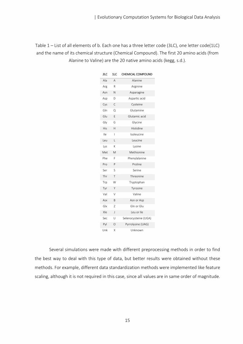
List of Tables Table 1 – List of all elements of b. Each one has a three letter code (3LC), one letter code(1LC)
and the name of its chemical structure (Chemical Compound). The first 20 amino acids (from
Alanine to Valine) are the 20 native amino acids (kegg, s.d.). .................................................... 15
Table 2 - Number of Proteins (positives) in each Subset for each class of Chou and Elrod 2003.
........................................................................................................................................................ 38
Table 3 – The increase in the average AUC value when used PSO-F, M equals to 10, k equals to
5, 100 iterations and with two different frequencies (and FC FNC) for 20 classes. .................. 45
Table 4 – Average AUC Values and Average Accuracy values obtained with different approaches
using Chou and Elrod 2003. For Pse-AAC λ was 10, Am-Pse-AAC λ was 9, and for the proposed
method was used PSO-F with M equal to 10, k equal to 5, MS-WSP, and 100 iterations. Also it
is present the improvement determined comparing to AAC and Am-Pse-AAC. ........................ 48
Table 5 - Average AUC Values and Average Accuracy values obtained with different approaches
using SCOP40mini. For Pse-AAC λ was 10, Am-Pse-AAC λ was 9, and for the proposed method
was used PSO-F with M equal to 10, k equal to 5, MS-WSP, and 500 iterations. Also it is present
the improvement determined comparing to AAC and Am-Pse-AAC. ......................................... 48
Table 6 – Principal SVM Classifiers parameters found in Search grid for Chou and Elrod 2003
set. .................................................................................................................................................. 49
Table 7 – The average number of features selected in each score in each class and set for Chou
and Elrod 2003 ............................................................................................................................... 50
Table 8 – Estimated running time (hour) for each step method per class. ............................... 51
Table 9 - The number and percentage (Rate) of positives in train and test sets for each class
considering the number of negatives in SCOP40mini dataset. ................................................... 61

xii

xiii
List of Figures Figure 1 – Representation of the different structures that a protein can assume illustrated by
the catabolite activator protein (Petsko & Ringe, 2004) ............................................................... 2
Figure 2 – Schematic Representation of the first three tier sequence order correlation mode
along a protein sequence on a Pse-AAC algorithm. ...................................................................... 8
Figure 3 - Pseudo Code of the Particle Swarm Optimization Algorithm used for feature Selection
(ist, s.d.) .......................................................................................................................................... 28
Figure 4 – Initial C# Application window ...................................................................................... 32
Figure 5 – Task Menu Panel .......................................................................................................... 33
Figure 6 – Scoring and MaxScoring Panel .................................................................................... 34
Figure 7 – Initial Menu Shown in Website ................................................................................... 35
Figure 8 – The available information about the used methods in Website ............................... 35
Figure 9 – Distribution of AUC values for some classes using different types of MaxScoring with
PSO-W, M equals 10, k equals 5, 100 iterations and with FC. .................................................... 42
Figure 10 - Distribution of AUC values for classes using different types of PSO, with MS-WPS, M
equals 10, k equals 5, 100 iterations and with FC. ...................................................................... 43
Figure 11 - Distribution of AUC values for each class using different M values, with MS-WPS,
PSO-F, k equals 5 and with FC. ...................................................................................................... 44
Figure 12 - AUC Values obtain in each class with different approaches using Chou and Elrod
2003. For Pse-AAC λ is 10, and Am-Pse-AAC λ is 9, for the new method is PSO-F with M equal
to 10, k is 5, MS-WSP and 200 iterations. .................................................................................... 46
xiv
Figure 13 - AUC Values obtain in each class with different approaches using SCOP40mini. For
Pse-AAC λ is 10, and Am-Pse-AAC λ is 9, for the new method is PSO-F with M equal to 10, k is 5,
MS-WSP, and 200 iterations without search grid. ....................................................................... 47

xv
List of Symbols 𝒂𝒎 Native amino acids
𝒂𝒎𝒏 m amino acid in n position
𝒃𝒎 Amino Acid m of the set with all coding possibilities of a sequence
𝒃𝒎𝒏 Amino Acid m of the set with all coding possibilities of a sequence at n
position in a sequence
𝒇𝒄 Frequency of consecutives elements
𝒇𝒏𝒄 Frequency of non-consecutive elements
𝒇𝒊(𝑷𝒋) Frequency of Amino Acid i in Protein j
𝒇𝒖 Normalized frequency of the 20 amino acid in a certain protein
sequence
𝐇𝟏 Hydrophobicity correlation function
𝒉𝟏 Amino acid hydrophobicity value
𝑯𝟏𝟎 Amino acid hydrophobicity value
𝑯𝟏(𝒊) Amino acid i hydrophobicity value after standardization
𝐇𝟐 Hydrophilicity correlation function
𝒉𝟐 Amino acid hydrophilicity value
𝑯𝟐𝟎 Amino acid hydrophilicity value
𝑯𝟐(𝒊) Amino acid i hydrophilicity value after standardization
𝑳 Sequence Length
𝝀 Total Number of order correlation factor
𝑴𝟎 Mass of an amino acid

xvi
𝑴(𝒊) Mass of i amino acid after standardization
𝑵 Total Number of samples in a set of proteins
𝑷𝒋(𝒏) Protein j
𝒔𝒄𝟐 Variance of subsequence FC
𝑺𝒌𝒊 Subsequence i with k amino acids in 𝑉(𝑖)
𝒔𝒏𝒄𝟐 Variance of subsequence FNC
𝜽𝒋 j-tier sequence correlation
𝑽(𝒊) All subsequences possible
𝒘 Weight factor for Pse-AAC and Am-Pse-AAC
𝒙𝒋⃗⃗ ⃗ AAC vector for Protein j
𝒙𝒖 Pse-AAC and Am-Pse-AAC vector for the representation of a certain
Protein

xvii
List of Abbreviations
AAC Amino Acid Composition
AFP Absolute Frequency by Presence
AFPC Absolute Frequency by Presence of Elements Arranged Consecutively
AFPN Absolute Frequency by Presence of Elements Arranged Non
Consecutively
Am-Pse-AAC Amphiphilic Pseudo Amino Acid Composition
ASF Absolute Set Frequency
ASFC Absolute Set Frequency of Elements Arranged Consecutively
ASFN Absolute Set Frequency of Elements Arranged Non Consecutively
AUC Area Under Curve
FC Frequency of Elements Arranged Consecutively
FNC Frequency of elements arranged non consecutively
FS Fisher Score
FSC Fisher Score of elements arranged consequently
FSN Fisher Score of elements arranged non consequently
KF k-Frequency
KFC K-Frequency of elements arranged consequently
KFN K-Frequency of elements arranged non consequently
MS MaxScoring
MS - N MaxScoring Normal

xviii
MS – WPS MaxScoring Without Parent Subsequences
Pse-AAC Pseudo Amino Acid Composition
PSO Particle Swarm Optimization
PSO-F Particle Swarm Optimization Features
PSO-W Particle Swarm Optimization Weights
PSO-WF Particle Swarm Optimization Weights and Features
RFP Relative Frequency by Presence
RFPC Relative Frequency by Presence of Elements Arranged Consecutively
RFPN Relative Frequency by Presence of Elements Arranged Non
Consecutively
SVM Support Vector Machine
TF-idf Term frequency–inverse document frequency
TFC-idf Term frequency–inverse document frequency of Elements Arranged
Consecutively
TFN-idf Term frequency–inverse document frequency of Elements Arranged
Non Consecutively
XS Qui quadrado statistics

| Evolutionary Computation Systems for Biological Data Analysis
1
1| Introduction
In this chapter, it is described the motivation, main objectives and the key concepts
about proteins and their importance. It will be referred only the most important aspects that
can influence the biochemical functions in a protein, like the presence of domains and motifs
as well their structure. Also, it is presented a brief overview of the chapters in a comparative
scheme.
1.1 | Motivation
The technological advances in the genomic and proteomic sequencing, headed to a
large increase of available data whose analysis may leads to discoveries in some areas, such as
pharmaceuticals or medicine. This rises the need to create computational tools able to
interpret different biological data, in this case proteins. Proteins are present in all cellular
metabolic reactions by performing a large number of several functions, so it’s important to
identify their biological purpose based on the data available in order to not require additional
laboratory work in researches with the study of proteins involved.
1.2 | Objectives
The main objective of this thesis is the design of a new method capable of predicting if
a protein belongs or not to a class or subclass of proteins, as well as being capable of it effective
regardless of the data set supplied.

1| Introduction
2
Therefore, all the research is the definition of a possible solution to a problem: the
prediction of a protein’s biochemical function through its primary structure.
1.3 | Proteins
Proteins are macromolecules formed by amino acids joined by peptides bonds. The
sequence of amino acids is determined by the sequences of nucleotide on a process called
translation (Campbell, 1996) after a gene as coded to pre-mRNA (Transcription). The sequence
of amino acid only is the primary structure of a protein.
The following sections will explain some of the elements that can determine or influence
the proteins’ biochemical functions as well as the functions themselves.
1.3.1 | Structures
As it is shown in figure 1, a protein can assume four different structures: Primary,
secondary, tertiary and quaternary. The first one is the sequence of amino acids and second is
the polypeptide chain taking the form of alpha helices or beta strands because of hydrogen
bonds processed between specific molecular groups of certain amino acids. In the tertiary
structure elements of either alpha helix or beta sheet or both, as well loops and links with no
secondary structures are folded into a globular form. At last, the quaternary structure is the
association of folded chains with more than one polypeptide.
Figure 1 – The different structures which a protein can assume illustrated by the catabolite activator protein (Petsko & Ringe, 2004)
The structure of a protein is important because in order for a polypeptide to function
as a protein in most cases must have a stable tertiary structure under physiological conditions.

| Evolutionary Computation Systems for Biological Data Analysis
3
Regarding the amino acids, they have different side chains which allows them to interact
differently with each other and with water. These differences affect their contributions to the
protein’s stability as well to the protein’s function. So, the amino acids are categorized as the
side chains present in them: hydrophobic, hydrophilic and amphipathic amino acids residues.
Also, certain amino acids are easier found or present in a greater amount in some
structures than others. It is the case of leucine and glutamine, which are often found in helices
in contrast to valine or isoleucine that are more often in beta sheets. But there also exceptions,
like the proline presence does not favor any kind of secondary structure. This is because each
side chains of each amino acid are essential for the chemical reactions needed for a protein to
assume any kind of form. As for the tertiary structure, most proteins can be unfolded or
refolded according to the diluted solution that they are in, indicating that the primary structure
contains all the information needed to specify the folded state.
In addition, the water molecules present on the surface of folded protein and the
possible bonds created also determines how a protein can be folded, since as referred before,
there are different types of amino acids and therefore different kinds of interactions between
amino acids and water. So, the side chains of amino acid will be arranged accordingly to the
presence of water molecules, the hydrophilic side chains will be arranged to be closer to water
molecules and the hydrophobic side chains will settle in the opposite way.
1.3.2 | Protein Domain
A domain is a specific region of a protein structure usually composed by a subsequence
of amino acids and is capable of existing on its own in aqueous solution. This segment holds
part of the biochemical function of the protein they belong to.
Not all the known domains are continuous segments of amino acids, in many proteins a
domain is divided and dispersed across the sequence and also they vary in size, being able to
contain an average of 200 amino acids, in which the smallest domain was registered with 57
amino acids and the biggest with 907 residues.

1| Introduction
4
1.3.3| Motifs
A motif can be a particular amino acids sequence that is present for a precise biological
function, or can be a set of contiguous secondary structure elements that either retain a
specific functional importance of a portion of a folded domain. In this sense, it can exist
functional motifs (like the ones found in DNA-binding proteins), or simpler structural motifs.
This last one does not exist separately from a protein and it can be used as a recognition
element for a group of similar proteins. A lot of structural motifs are found in many hormones
as well as proteins with NAD cofactors.
The recognition of a motif in a sequence is not easy since most of sequence motifs are
discontinuous and the space between their elements can vary significantly and this makes them
easier to detected from a structure view rather than from the amino acids sequence. As for the
structural motifs, its identification only from the sequence is very difficult given that many
different amino acids can lead to same secondary structure making algorithms based in
similarity alone not enough.
1.3.4 | Biochemical Functions
The different protein biochemical functions can be categorized into four main functions:
binding, catalysis, switching and as structural elements. In binding, proteins bind to a specific
or more substrates like Myoglobin binds a molecule of oxygen reversibly to the iron atom in its
heme. As for the second category, the proteins are responsible to increase the velocity of every
chemical reaction in a living cell. Switching proteins are flexible molecules and their
conformation change with ph or a ligand binding, allowing some cellular processes to be
controlled. These conformational changes are crucial for the molecular basis of many cancers
like the ones that occurs in the GTPase Ras1 when GTP2 is hydrolyzed to GDP3. At last, structural
proteins give strength or toughness to living systems, and they depend on specific protein
subunits with other proteins or molecules.
1 Protein from a large family of hydrolase enzymes that can bind and hydrolyze guanosine triphosphate, this particular protein is a member of the Ras superfamily of proteins 2 Guanosine triphosphate 3 Guanosine diphosphate

| Evolutionary Computation Systems for Biological Data Analysis
5
1.4 | Thesis Structure
This thesis has six distinctive chapters. In chapter 2 a synopsis of related works is
presented. In chapter 3 all the implemented methods, as well the new method, are explained.
In chapter 4, it is presented an application and a website created to implement the different
methods described before. In chapter 5, it is introduced the different results as they are
discussed in chapter 6. At last, the final remarks, conclusions and suggestions for future work
are present in chapter 7.

1| INTRODUCTION
6
1| INTRODUCTION

| Evolutionary Computation Systems for Biological Data Analysis
7
2| Literature Review
In this chapter, it will be referenced and discussed the several researchs carried out
using the primary sequence of a protein to create models that can predict their biochemical
functions.
2.1 | Chapter Introduction
There are several factors that can determine or influence the action of a protein in a
cell, from its sequence, structure, cellular location, and or even to the presence of other
proteins. Thus, several studies address the same problem in different ways: either by predicting
subcellular location of a group of proteins or the enzymes subclasses.
So this subject can be divided into three sub problems: protein representation or
feature extraction, feature selection and the prediction algorithms used.
2.2 | Features Extraction
The representation of a protein sequence is one of the most important tasks as it may
determine the success of any model. It is important that a protein is mathematically well
represented in order to have the greatest number of critical information which can characterize
it between a set of proteins that share the same function. However, we only have access to a
sequence of amino acids, so it is necessary to implement methods to extract features from it.
For this purpose, there are also different approaches: methods based on AAC, subsequences,
and N-terminal targeting.

2| Literature Review
8
One of the most basic ways to represent a protein sequence is by counting the 20 amino
acids in the sequence: AAC (Nishikawa, et al., 1983). Despite being a fairly simple and old
method, it is still used quite successfully in several sets of proteins to predict their subcellular
location or subfamily (Zhou & Doctor, 2003), or as a way to establish a performance threshold
when proposed a new method with a new set of proteins (Yang, 2011). However, the simplicity
of AAC means that many important factors for a biochemical function are not represented.
Pse-AAC technique was developed by Kuo Chen Chou (Chou, 2001) and this method
brought something new and unique to the approaches previously used (variations of AAC) to
predict cell attributes. Chou showed a new representation of protein sequences, in which was
still present in the frequency of the 20 amino acids, as well as their mass, hydrophobicity and
hydrophilicity according to the order they appear in the same sequence. Thus, not could only a
new interpretation for the first time took account of some chemical properties as well as the
order in which the amino acids appeared in the sequence. In addition, using this method a
protein sequence is analyzed as set of amino acid pairs (figure 2), because the terms
determined to implement this method always needs the current and the immediately following
amino acid. In his first work, Chou had used the Pse-AAC to predict cell locations, however this
method of feature extraction has been used for other purposes such as prediction of protein
structures (Sahu & Panda, 2010), potentially allergenic proteins (Mohabatkar et al., 2013),
families of human enzymes (Wu, et al., 2016), among many other studies in various topics.
Figure 2 – Schematic Representation of the first three tier sequence order correlation mode
along a protein sequence on a Pse-AAC algorithm.
The Pse-AAC was also used in predicting 16 different oxygenase classes according to
different target groups (Elrod & Chou, 2003). This work was important in the sense that it
determined the homologies between the proteins of each class in order to understand how this

| Evolutionary Computation Systems for Biological Data Analysis
9
factor could be decisive when using methods based on the AAC. And it proved that despite low
homology (30%) between proteins in the same class, with Pse-AAC was able to obtain an
accuracy values above 70%, demonstrating that with only the primary sequence is possible to
identify and predict a set of proteins with different sequences, whether by class families or their
subcellular location.
After the initial proposal of Chou, different variations of his work appeared in order to
complete the representation with more relevant biological information, it was the case of isno-
PseAAC (Xu et al., 2013), a new approach to Pse-AAC, allowing the incorporation of a factor
called the propensity of the position of a specific amino acid to predict Cysteine S-nitrosylation
Sites in Proteins. Basically, it is a 21x20 matrix in which each row and column represent the 20
amino acids and the possibility of encoding not one, i.e. the existence of an element x in an
amino acid sequence. Thus each element of the array can be translated in the interaction of
two consecutive amino acids in the sequence, where is calculated the difference between the
terms Pse-AAC for a pair of amino acids between the data set that contains peptide fragments
and those that don’t.
Besides Pse-AAC, Chou also proposed Am-Pse-AAC to predict enzyme subclasses, in
which the molecular weight is not considered and hydrophobicity and hydrophilicity are
considered differently in the correlation coefficients, more detail in next chapter (Chou, 2004).
The Am-Pse-AAC was also incorporated in different works related to the study of iterations
between proteins (Huang, et al., 2014).
It is important to add that all these methods were used for feature extraction, due to
the fact that is only based on an amino acid sequence, the same methods were transposed of
different biological data, like for RNA sequences (Liu, et al. 2015), and DNA small sequences
(Liu et al., 2015).
As for Pse-AAC, it proved to be an effective and simple method to represent a protein
leading to the existence of many diverse research, as mentioned earlier. However, it cannot
be ignored some aspects that can make this an inadequate protein representation.
Firstly, the protein is observed as a set of pairs, so it is not taken in consideration the
existence of protein domains, subsequences crucial to its structure as well as biochemical
functionality. Another aspect, it is related to the use of hydrophilicity and hydrophobicity,

2| Literature Review
10
important parameters for intra and inter molecular interactions in the various activities of a
protein, as another identification to an amino acid. But instead of having the designation of the
single letter amino acid, it has a term that considerers its mass, hydrophilicity and
hydrophobicity. Lastly, the protein is not fully analyzed, despite being present the total
frequency of each amino acid sequence, the order is considered to a certain amino acid in the
sequence, so possible vital information is not considered.
In addition to the above mentioned methods there is the analysis of amino acids
sequences present in the protein primary structure through its presence and / or its frequency.
Such subsequences can be different combinations of amino acids set (k-tuples), motifs
sequences or N-terminal targeting sequences (small peptides present in the protein
responsible for the migration of the protein into all specific organelle, such a mobile locator.
(Hoglund et al., 2005) (A, et al., 2006).
The biggest problem in using motifs sequences or N-terminal targeting sequences is that
it is limited because it is needed a prior knowledge of the type of proteins used and the
laboratorial technique performed, and also exist many cellular events that can change or
mutate these subsequences.
However, the use of k-tuples is positive in the sense that for the chosen data set is done
a thorough search for subsequences that may be potential motifs, targeting sequences or
domains. Though, given the existing amino acids and the number of all possible combinations,
the number of the all possible subsequences leads to a very high number of potential attributes
that can serve as feature to train a classifier. Not to mention that assessment of these same
subsequences only by the presence or frequency continues to be insufficient in relation to the
biological and chemical knowledge of the subject. It is not only the presence or frequency of a
pattern that influence the structure and thereby the biochemical functionality of a protein.
Because there are several intra and inter molecular interactions or structures of each amino
acid set in the same sequence that can determine different biological purposes for a certain
protein.

| Evolutionary Computation Systems for Biological Data Analysis
11
2.3 | Feature Selection
After the features extraction is set, how those features are going to be selected is also
important, since any efficient prediction model depends on how well described is our study
object.
And for proteins, it is even more difficult to choose a correct way of features selection
because of the enormous number of biological variables that may contribute to its classification
presence in a particular cellular location, or as belonging to a group of proteins that share the
same chemical or functional characteristic.
In several researches, there are different methods for features selection, in which some
used using the analysis of subsequences of amino acids (k-tuples). There are studies that select
k-tuple more frequently, or with higher discriminative power or less independent, by
calculating its frequency, Fisher's criterion, the quadratic chi respectively (Yang et al., 2006)
(Yiming Yang, 1997). After, the attributes of each metric were evaluated separately in order to
realize which is most efficient in the feature selection.
Another feature selection process is by homology analysis of these k-tuples with the
proteins belonging to a particular class. In this process are chosen the subsequences that
present the highest similarity with the referred proteins (Tian & Skolnick, 2003).
It is also important to note that many studies already used variations of the Particle
Swarm Optimization (Kennedy & Eberhart, 1995) to select a set of attributes according to a
chosen parameter as a fitness function, like with Chieh-Yuan´s work (Tsaia & Chena, 2015), in
which the PSO was used to choose a set of k-tuples using as fitness function their similarity with
positive proteins (proteins that belong to a class).
In others researches the PSO is used to find the attributes that lead to better an accuracy
value when applied different types of predicting algorithms, having as features the terms of the
Pse-AAC (Bagyamathi & Inbarani, 2015) (Mandal et al., 2015) (Bin Liu, 2015).

2| Literature Review
12
2.4 | Prediction Algorithms
The last factor that contributes to the success of a prediction model is the selection of
a prediction algorithm. If is for the prediction of enzymes’ subclasses or for identifying
subcellular locations different methods were applied.
The nearest-neighbor method is used in a wide variety of researches to predict enzymes
or to predict the types of membrane proteins (Shena & Choua, 2005).
Another prediction algorithm used is SVM, in which from protein sequences and defined
attributes can determine whether a protein belongs to a class by the characterization of a
hyperplane that maximizes the margin that separate two types of data, in this a case is if a
sequence belongs or not to a class of proteins (Zhou et al., 2007) (Annette Hoglund, 2006).
Other methods applied were mining association and Bayesian classification rules, in
which it was possible to identify different classes of enzymes with rules associated with the
protein domain composition (Guda, 2011).
2.5 | Conclusion
For Feature Extraction exist effective methods from protein sequences, however there
are always important chemical functionality factors of a protein being ignored or not shown. In
Pse-AAC a protein is not fully analysed, while the others methods are based on similarity with
known subsequences, therefore not successful for class proteins sets with low homology,
mutated proteins or with lost motifs sequences. And some feature selection methods conduct
an analysis based only on one factor or parameter.
2.6 | Our Proposal
Based on what it was referred before, it was created a method that from all possible
combinations of variable size subsequences are pre-selected (according to more than 24
different metrics) to build a search space used in PSO to select some of them to increase the
AUC (area under curve), creating a system capable of evaluating subsequences by different
parameters simultaneously.

| Evolutionary Computation Systems for Biological Data Analysis
13
3|Methods In this chapter, it will be discussed in detail the methods based on AAC which have been
implemented in detail, and also it will be described all the components and different variables
of the proposed method.
3.1 | Chapter Introduction
It is necessary to find variables or parameters capable of identifying a certain set of
proteins, in order to distinguish their different classes or subclasses to correctly identifying
them, which makes it possible to establish some of the main protein functions.
The biggest obstacle lies in determining correctly these same variables solely with the
protein sequence. Therefore, different methods were implemented to define diverse sets of
variables.
First, each set of proteins was characterized by the number of each amino acid (AAC).
Also, it was applied a method created by Kuo-Chen Chou (Pse-AAC) in which the amino acids’
arrangement on the protein sequence as well as their hydrophobicity, hydrophilicity, and mass
are taken in to consideration. Furthermore, all possible combinations of subsequences were
determined by a predefined number of amino acids present so they could be scored according

3|Methods
14
to their occurrence and other parameters in each protein sequence (Scoring), and then some
of them selected through the highest scores.
Additionally, it was implemented the PSO on all variables previously referenced in order
to select the variables best capable of characterizing a certain protein set.
3.1 | Amino Acid Composition – AAC
The Amino Acid Composition is the simplest way to attempt to solve this problem and
almost all the previous works made in this field are based on it, plus its results provided were
used to show how well a new algorithm can improve them.
Therefore, considering a certain set with N proteins, each protein j (𝑃𝑗) can be
represented as an array of L-amino acids (𝑏𝑚):
𝑃𝑗(𝑛) = 𝑏𝑚1…𝑏𝑚
𝑛𝑏𝑚𝑛+1𝑏𝑚
𝑛+2… 𝑏𝑚𝐿−2𝑏𝑚
𝐿−1𝑏𝑚𝐿 (1)
𝐿 > 0 , 1 < 𝑛 < 𝐿, 𝑚 > 0, 1 < 𝑗 ≤ 𝑁
where n indicates the amino acid position in the protein sequence, and m identifies an element
of b, assuming this contains all the coding possibilities, in a protein sequence, besides the 20
native amino acids because unknown or ambiguous amino acids may also exist.
For AAC, each protein j was represented by a vector (𝑥𝑗⃗⃗ ⃗) with 20 elements, each
corresponding to the number of occurrences of an amino acid in the same protein sequence
(𝑓𝑖(𝑃𝑗)), since this amino acid was one of the 20 native amino acids.
𝑥𝑗⃗⃗ ⃗ = [𝑓1(𝑃𝑗), 𝑓2(𝑃𝑗), … , 𝑓20(𝑃𝑗)] (2)
As a result, to train a possible model each sample was a protein sequence represented
by 20 features and labeled as 1 or 0, depending on whether they belong or not to a certain
class of proteins.
| Evolutionary Computation Systems for Biological Data Analysis
15
Table 1 – List of all elements of b. Each one has a three letter code (3LC), one letter code(1LC)
and the name of its chemical structure (Chemical Compound). The first 20 amino acids (from Alanine to Valine) are the 20 native amino acids (kegg, s.d.).
3LC 1LC CHEMICAL COMPOUND
Ala A Alanine
Arg R Arginine
Asn N Asparagine
Asp D Aspartic acid
Cys C Cysteine
Gln Q Glutamine
Glu E Glutamic acid
Gly G Glycine
His H Histidine
Ile I Isoleucine
Leu L Leucine
Lys K Lysine
Met M Methionine
Phe F Phenylalanine
Pro P Proline
Ser S Serine
Thr T Threonine
Trp W Tryptophan
Tyr Y Tyrosine
Val V Valine
Asx B Asn or Asp
Glx Z Gln or Glu
Xle J Leu or Ile
Sec U Selenocysteine (UGA)
Pyl O Pyrrolysine (UAG)
Unk X Unknown
Several simulations were made with different preprocessing methods in order to find
the best way to deal with this type of data, but better results were obtained without these
methods. For example, different data standardization methods were implemented like feature
scaling, although it is not required in this case, since all values are in same order of magnitude.

3|Methods
16
3.2 | Pseudo Amino Acid Composition – Pse-AAC
The main purpose of this methodology is to include more significant information than the
AAC by considering the physical and chemical properties of each amino acid present in a certain
protein sequence.
According to this method and equation present in 1, the order-correlated factor was
defined as:
{
𝜃1 =
1
𝐿−1∑ Θ(𝑃𝑗(𝑛), 𝑃𝑗(𝑛 + 1)𝐿−1𝑛=1 )
𝜃2 = 1
𝐿−2∑ Θ(𝑃𝑗(𝑛), 𝑃𝑗(𝑛 + 2)𝐿−2𝑛=1 )
𝜃3 = 1
𝐿−3∑ Θ(𝑃𝑗(𝑛), 𝑃𝑗(𝑛 + 3))𝐿−3𝑛=1
…
𝜃𝜆 = 1
𝐿−𝜆∑ Θ(𝑃𝑗(𝑛), 𝑃𝑗(𝑛 + 𝜆))𝐿−𝜆𝑛=1
(𝜆 < 𝐿) (4)
Subsequently, the correlation factors are determined considering the sequence order
correlation between continuous residues along the protein sequence. Therefore, the
correlation function was determined by:
Θ(𝑃𝑗(𝑛), 𝑃𝑗(𝑛 + 𝜆)) = 1
3{[𝐻1(𝑃𝑗(𝑛 + 𝜆)) − 𝐻1(𝑃𝑗(𝑛))]
2+ [𝐻2(𝑃𝑗(𝑛 + 𝜆)) −
𝐻2(𝑃𝑗(𝑛) =]2+[𝑀(𝑃𝑗(𝑛 + 𝜆)) −𝑀(𝑃𝑗(𝑛))]
2} (5)
In the prior mathematical expression, 𝐻1 is the amino acid hydrophobicity value, 𝐻2 is
the amino acid hydrophilicity value and 𝑀 its side-chain mass. These parameters were
converted by the following standardization:
{
𝐻1(𝑖) =
𝐻10(𝑖)−∑
𝐻10(𝑖)
2020𝑖=1
√∑ [𝐻10(𝑖)−∑
𝐻10(𝑖)
2020𝑖=1 ]
220𝑖=1
20
𝐻2(𝑖) = 𝐻20(𝑖)−∑
𝐻20(𝑖)
2020𝑖=1
√∑ [𝐻20(𝑖)−∑
𝐻20(𝑖)
2020𝑖=1 ]
220𝑖=1
20
𝑀(𝑖) = 𝑀0(𝑖)−∑
𝑀0(𝑖)
2020𝑖=1
√∑ [𝑀0(𝑖)−∑𝑀0(𝑖)20
20𝑖=1 ]
220𝑖=1
20
(6)

| Evolutionary Computation Systems for Biological Data Analysis
17
where 𝐻10 is the amino acid hydrophobicity value taken from Tanford research (C, 1962) , 𝐻20 is
the amino acid hydrophilicity value acquired by Hoop and Woods’ work (Hopp TP, 1981) and
𝑀0 the mass of an amino acid (biofor, s.d.).
Consequently, each protein was represented by the resulting vector:
𝑥𝑢 = {
𝑓𝑢
∑ 𝑓𝑖20𝑖=1 +𝑤∑ 𝜃𝑗
𝜆𝑗=1
(1 ≤ 𝑢 ≤ 20)
𝑤𝜃𝑢−20
∑ 𝑓𝑖20𝑖=1 +𝑤∑ 𝜃𝑗
𝜆𝑗=1
(20 + 1 ≤ 𝑢 ≤ 20 + 𝜆 (7)
In which 𝑓𝑢 is the normalized frequency of the 20 amino acid in a certain protein
sequence, 𝜃𝑗 the j-tier sequence correlation and 𝑤 the weight factor for the amino acid
arrangement effect.
3.3 | Amphiphilic Pseudo Amino Acid Composition – Am-Pse-AAC
This method is very similar to Pse-AAC, so the order-correlated factor was defined as:
{
𝜃1 =
1
𝐿−1∑ H1(𝑃𝑗(𝑛), 𝑃𝑗(𝑛 + 1)𝐿−1𝑛=1 )
𝜃2 = 1
𝐿−1∑ H2(𝑃𝑗(𝑛), 𝑃𝑗(𝑛 + 1)𝐿−1𝑛=1 )
𝜃3 = 1
𝐿−2∑ H1(𝑃𝑗(𝑛), 𝑃𝑗(𝑛 + 2)𝐿−2𝑛=1 )
𝜃3 = 1
𝐿−2∑ H2(𝑃𝑗(𝑛), 𝑃𝑗(𝑛 + 2)𝐿−2𝑛=1 )
…
𝜃2𝜆−1 = 1
𝐿−𝜆∑ H1(𝑃𝑗(𝑛), 𝑃𝑗(𝑛 + 𝜆))𝐿−𝜆𝑛=1
𝜃2𝜆 = 1
𝐿−𝜆∑ H2(𝑃𝑗(𝑛), 𝑃𝑗(𝑛 + 𝜆))𝐿−𝜆𝑛=1
(𝜆 < 𝐿) (8)
where H1 and H2 were the hydrophobicity and hydrophilicity correlation functions given by:
H1 (𝑃𝑗(𝑛), 𝑃𝑗(𝑛 + 𝜆)) = ℎ1(𝑃(𝑛)) . ℎ1 (𝑃𝑗(𝑛 + 𝜆)) (9)
H2 (𝑃𝑗(𝑛), 𝑃𝑗(𝑛 + 𝜆)) = ℎ2(𝑃(𝑛)) . ℎ2 (𝑃𝑗(𝑛 + 𝜆)) (10)
where, ℎ1 is the amino acid hydrophobicity value and ℎ2 is the amino acid
hydrophilicity value. Like for Pse-AAC, these parameters were converted by the following
standardization:

3|Methods
18
{
𝐻1(𝑖) =
ℎ10(𝑖)−∑
ℎ10(𝑖)
2020𝑖=1
√∑ [ℎ10(𝑖)−∑
ℎ10(𝑖)
2020𝑖=1 ]
220𝑖=1
20
𝐻2(𝑖) = ℎ20(𝑖)−∑
ℎ20(𝑖)
2020𝑖=1
√∑ [ℎ20(𝑖)−∑
ℎ20(𝑖)
2020𝑖=1 ]
220𝑖=1
20
(11)
where ℎ10 is the amino acid hydrophobicity value taken from Tanford research (C, 1962) and
ℎ20 is the amino acid hydrophilicity value acquired by Hoop and Woods’ work (Hopp TP, 1981).
Consequently, each protein was represented by the resulting vector:
𝑥𝑢 = {
𝑓𝑢
∑ 𝑓𝑖20𝑖=1 +𝑤∑ 𝜃𝑗
𝜆𝑗=1
(1 ≤ 𝑢 ≤ 20)
𝑤𝜃𝑢
∑ 𝑓𝑖20𝑖=1 +𝑤∑ 𝜃𝑗
𝜆𝑗=1
(20 + 1 ≤ 𝑢 ≤ 20 + 2𝜆 (12)
In which 𝑓𝑢 is the normalized frequency of the 20 amino acid in a certain protein
sequence, 𝜃𝑗 the j-tier sequence correlation and 𝑤 the weight factor for the amino acid
arrangement effect.
3.3 | Scoring
As referred in the last chapter, in this process different subsequences (k-tuples) were
designated as possible variables capable of specifying a protein’s a class. However, considering
all the possible combinations of subsequences, this process can lead to many computational
problems. One of the ways found to overcome this difficulty is to assign statistical significance
to each of the variables created. In order to do so, different metrics (scores) were determined
to specify several degrees of importance in the same variable on a sample or set, each sample
being a protein and each variable a k-tuple.
There were several types of scores already applied in previous studies, such as the
frequency of a k-tuple on a set of proteins, the linear Fisher discriminant or 𝜒2 statistics.
Nevertheless, considering the different forms of chemical interactions that may occur
in a protein in different sections of its primary structure, other basic metrics can lead to the
selection of other k-tuples essential to the correct class prediction. For example, proteins

| Evolutionary Computation Systems for Biological Data Analysis
19
belonging to different classes may differ by the presence or absence of a certain subsequence,
the number of copies of it, as well as its subsequence position in the sequence.
As a result, different scores were defined to approach the problem, so the variables may
be selected to assess which factor weighs more in the deference between the proteins
belonging or not to a class, and to reduce the space search of all possible variables.
3.3.1 | k-tuples
So, one way to extract potential features from the protein sequence is through k-tuples,
smaller subsequences with k-amino acids. Basically by defining a k, all possible combinations
from 2 to k with the 20 native amino acids were found computationally to proceed to scoring.
Thus, considering a space with all k-tuples variables as 𝑉(𝑖), which its dimension is equal
to ∑ 20𝑛𝑘𝑛=1 , each element is 𝑆𝑘𝑖, an amino acid subsequence with k-amino acids (𝑎𝑚) was
exemplified as:
𝑆𝑘𝑖(𝑛) = 𝑎𝑚1𝑎𝑚
2… 𝑎𝑚𝑛 … 𝑎𝑚
𝑘 (13)
𝑎𝑚 ∈ 𝑎 = {20 𝑛𝑎𝑡𝑖𝑣𝑒 𝑎𝑚𝑖𝑛𝑜 𝑎𝑐𝑖𝑑𝑠∗}
2 ≤ 𝑘 ≤ 5 , 𝑖 ∈ ℕ+, 1 < 𝑛 < 5
where n indicates the amino acid position the subsequence, and m identifies an element of a,
supposing it has all native 20 amino acids.
3.3.2 | Frequency
In order to define different scores, initially two distinct subsequence frequencies were
formulated: frequency of elements arranged consecutively and frequency of elements
arranged non consecutively.
This distinction was made because a specific subsequence 𝑆𝑘𝑖 may be crucial to identify
the protein function (first frequency), given that a protein sequence may have unknown or
ambiguous amino acids and in the different protein structures can occur several chemical
interactions between distant groups of amino acids (second frequency).

3|Methods
20
3.3.2.1 | Frequency of Elements Arranged Consecutively - FC
Thus, the frequency of a k-tuple variable 𝑆𝑘𝑖 with n elements arranged consecutively on
a protein 𝑃𝑗 was defined by:
𝐹𝐶(𝑃𝑗 , 𝑆𝑘𝑖) = ∑ [𝑓𝑐(𝑃𝑗[𝑛: 𝑛 + 𝑘], 𝑆𝑘𝑖), 𝑎𝑚1 = 𝑏𝑚
𝑛]𝐿−𝑘+1𝑛=1 (14)
𝑓𝑐(𝑃𝑗[𝑛: 𝑛 + 𝑘], 𝑆𝑘𝑖) = {1, ∃𝑎𝑚
𝑑 = 𝑏𝑚𝑐
0, ∃ 𝑎𝑚𝑑 ≠ 𝑏𝑚
𝑐 𝑑 = 𝑐 − 𝑛, ∀ (𝑃𝑗[𝑛: 𝑛 + 𝑘], 𝑆𝑘𝑖)(10)
The frequency of n elements arranged consecutively is the number of events that all the
amino acids of 𝑆𝑘𝑖 are disposed in the designated order and consecutively in the protein
sequence 𝑃𝑗. By analyzing 𝑃𝑗, when an amino acid (𝑏𝑚𝑛) in n positon is equal to the first amino
acid (𝑎𝑚1) of 𝑆𝑘𝑖, it is checked whether the immediately remaining subsequent amino acids of
𝑃𝑗 match the same order to the last amino acid of the 𝑆𝑘𝑖. In this case, it must be beaded 1 to
the current frequency and the next the amino acid to analyze in 𝑃𝑗 is located at n + k + 1. If not,
the next amino acid to be evaluated has n+1 position.
3.3.2.1 | Frequency of elements arranged non consecutively - FNC
Given the previous principles, for a protein 𝑃𝑗 it is possible to determine the frequency
of elements arranged non consecutively in the following:
𝐹𝑁𝐶(𝑃𝑗 , 𝑆𝑘𝑖) = ∑ [𝑓𝑛𝑐(𝑃𝑗[𝑛: 𝐿], 𝑆𝑘𝑖), 𝑎𝑚1 = 𝑏𝑚
𝑛]𝐿−𝑘+1𝑛=1 (15)
𝑓𝑛𝑐(𝑃𝑗[𝑛: 𝐿], 𝑆𝑘𝑖) = {1, ∃ 𝑎𝑚
𝑑 = 𝑏𝑚𝑐
0, ∄ 𝑎𝑚𝑑 = 𝑏𝑚
𝑐 , 𝑑 ≤ 𝑐 − 𝑛 , ∀ 𝑆𝑘𝑖 (16)
So, in 𝑃𝑗 when an n amino acid (𝑏𝑚𝑛) is equal to the first amino acid (𝑎𝑚1) of 𝑆𝑘𝑖, it
continues to search for the second amino acid 𝑎𝑚2 in 𝑃𝑗 located after 𝑏𝑚𝑛 regardless the
position of the same amino acid may occupy. The current frequency will increase by one when
all 𝑆𝑘𝑖’s amino acids are found on the sequence protein in the same order they are presented.
After, the search for 𝑎𝑚1 in 𝑃𝑗 begins again at the amino acid following the first one found
before, and all the amino acids once considered are ignored on the succeeding searches.
The way this frequency is defined, the elements of 𝑆𝑘𝑖 arranged consecutively in the
protein sequence are also being considered, but in less number.
| Evolutionary Computation Systems for Biological Data Analysis
21
3.3.3 | Data Sets
To correctly evaluate the k-tuples found, and select the best representative features,
three sets were created in which each subsequence is evaluated: The set of proteins that will
be used to train a model (data_all), the set with the proteins which in the previous set belong
to the class (data_pos) and another set with proteins which are not part of it (dara_neg). By
doing so, it is possible to review the different k-tuples without the scores being excessively
influenced by the unbalance between the number of proteins from the class and the number
which do not belong. There isalso a possible way to clearly find the features that best
characterize each case.
3.3.4 | Scores
Diverse categories of scores were created in order to analyze each subsequence (𝑆𝑘𝑖)
considering different characteristics, such as its number of elements (𝑎𝑚), its frequency in a
defined protein set, how discriminant it is for different types of proteins, among others.
3.3.4.1 | Absolute Set Frequency – ASF
This score is the simplest way to evaluate the significance of a subsequence on a certain
protein set. Basically, it determines how important a subsequence is by measuring its frequency
on each protein. Some repeated subsequences can be important in a protein structure and
consequently in its metabolic function.
For the subsequence 𝑆𝑘𝑖 and certain set with N proteins, this score was the sum of the
subsequence frequency in each protein as it is defined next.
3.3.4.1.1 | Absolute Set Frequency of Elements Arranged Consecutively – ASFC
𝐴𝑆𝐹𝐶(𝑆𝑘𝑖) = ∑ 𝐹𝐶(𝑃𝑗 , 𝑆𝑘𝑖)𝑁𝑗=1 (17)
3.3.4.1.2 | Absolute Set Frequency of Elements Arranged Non Consecutively – ASFN
𝐴𝑆𝐹𝑁(𝑆𝑘𝑖) = ∑ 𝐹𝑁𝐶(𝑃𝑗 , 𝑆𝑘𝑖)𝑁𝑗=1 (18)

3|Methods
22
3.3.4.2 | Absolute Frequency by Presence – AFP
This score evaluates whether a certain subsequence is present or not in a protein
sequence, rather than its frequency. Consequently, the score will be higher the more proteins
has the subsequence in question. This score was defined this way because a certain k-tuple can
be very common in some proteins, however, it is not expressed significantly throughout the
defined set or by its frequency in the sequence.
So, for a set with N proteins, a subsequence (𝑆𝑘𝑖) will have as a score the number of
proteins in which it had a frequency higher than 0. This score was used in order to take into
consideration the two types of frequency.
3.3.4.2.1 | Absolute Frequency by Presence of Elements Arranged Consecutively – AFPC
For a certain subsequence 𝑆𝑘𝑖 the Absolute Frequency by Presence of Elements
Arranged Consecutively is determined by:
𝐴𝐹𝑃𝐶𝑖(𝑆𝑘𝑖) = ∑ 𝐸𝑐𝑁𝑗=1 (𝑃𝑗 , 𝑆𝑘𝑖) (19)
𝐸𝑐(𝑃𝑗 , 𝑆𝑘𝑖) = { 1 , 𝑖𝑓 𝐹𝐶(𝑃𝑗 , 𝑆𝑘𝑖) > 0
0 , 𝑖𝑓 𝐹𝐶(𝑃𝑗 , 𝑆𝑘𝑖) = 0 (20)
In which N represents the total number of proteins in a defined set, 𝑃𝑗 is one of those proteins.
3.3.4.2.2 | Absolute Frequency by Presence of Elements Arranged Non Consecutively – AFPN
The AFPN is defined by:
𝐴𝐹𝑃𝑁(𝑆𝑘𝑖) = ∑ 𝐸𝑛𝑐𝑁𝑗=1 (𝑃𝑗 , 𝑆𝑘𝑖) (21)
𝐸𝑛𝑐(𝑃𝑗 , 𝑆𝑘𝑖) = { 1, 𝑖𝑓 𝐹𝑁𝐶(𝑃𝑗 , 𝑆𝑘𝑖) > 0
0, 𝑖𝑓 𝐹𝑁𝐶(𝑃𝑗 , 𝑆𝑘𝑖) = 0 (22)
3.3.4.3 | Relative Frequency by Presence – RFP
This score is similar to the last one, the difference is that RFP takes into account the
number of proteins in the defined set. Of course, in MaxScoring the previous score and RFP will
lead to the selection of the same sequences in data_all. However, this score was not created

| Evolutionary Computation Systems for Biological Data Analysis
23
to be used in data_all, but rather to create a different selection for the remaining sets, which
shall be addressed in the next section with a more detailed description of MaxScoring.
Also the two types of frequency were considered, therefore the two types of scores shall be
described next.
3.3.4.3.1 | Relative Frequency by Presence of Elements Arranged Consecutively – RFPC
𝑅𝐹𝑃𝐶(𝑆𝑘𝑖) = 1
𝑁∑ 𝐸𝑐𝑁𝑗=1 (𝑃𝑗 , 𝑆𝑘𝑖) (23)
𝐸𝑐(𝑃𝑗 , 𝑆𝑘𝑖) = { 1 , 𝑖𝑓 𝐹𝐶(𝑃𝑗 , 𝑆𝑘𝑖) > 0
0 , 𝑖𝑓 𝐹𝐶(𝑃𝑗 , 𝑆𝑘𝑖) = 0 (24)
3.3.4.3.2 | Relative Frequency by Presence of Elements Arranged Non Consecutively – RFPN
𝑅𝐹𝑃𝑁(𝑆𝑘𝑖) = 1
𝑁∑ 𝐸𝑛𝑐𝑁𝑗=1 (𝑃𝑗 , 𝑆𝑘𝑖) (25)
𝐸𝑛𝑐𝑗(𝑆𝑘𝑖) = { 1, 𝑖𝑓 𝐹𝑁𝐶𝑗(𝑆𝑘𝑖) > 0
0, 𝑖𝑓 𝐹𝑁𝐶𝑗(𝑆𝑘𝑖) = 0 (26)
3.3.4.4 | k-Frequency – KF
It would be incorrect to evaluate the frequency of the variables disregarding the length
of each one. The more amino acids the variable has, the lower its frequency is comparing to
the features of AAC. In this sense, to try a solution, this score was created, which attempts to
benefit variables with more elements, or at least to enable their evaluation more evenly.
Therefore, KF is the ratio between the sum of a subsequence frequency in each protein
and k, variable defined when all k-tuples were defined. [see 3.1 k-tuples]
In this score, both frequencies were used like it is shown below.
3.3.4.4.1 | K-Frequency of elements arranged consequently – KFC
𝐾𝐹𝐶(𝑆𝑘𝑖) = ∑𝐹𝐶(𝑃𝑗,𝑆𝑘𝑖)
k
𝑁𝑗=1 (27)
3.3.4.4.2 | K-Frequency of elements arranged non consequently – KFN
𝐾𝐹𝑁(𝑆𝑘𝑖) = ∑𝐹𝑁𝐶(𝑃𝑗,𝑆𝑘𝑖)
k
𝑁𝑗=1 (28)

3|Methods
24
3.3.4.5 | Fisher Score – FS
This score is based on the Fisher linear discriminant analysis, a method used in pattern
recognition, machine learning, and other fields of expertise, to find a linear combination of
features that characterizes and/or separates two or more classes of objects or events.
Considering a class of proteins, it was defined that the two events assessed would be if the
protein belongs (labeled as 1) or not to the same class (labeled as 0).
In previous works, the same score was used in order to find the discriminating variables
between different protein classes with extended formulas, but in this case the way that all sets
and classes are defined is not possible to do the same, and also before knowing what features
separate different classes, it is more important to know what subsequences can characterize a
protein in a way to show if it belongs or not to a certain class, since, proteins share similar
characteristics when it comes to their functionality: some have multiple functions, and
therefore, multiple classes.
Accordingly, for a certain set of N protein, FS of a certain subsequence 𝑆𝑘𝑖 is a ratio in
which the numerator is the square of the difference between the mean frequency of 𝑆𝑘𝑖 in
proteins labeled as 1 and 0, and the denominator is the sum of the variances of those
frequencies.
3.3.4.5.1 | Fisher Score of elements arranged consequently – FSC
𝐹𝑆𝐶(𝑆𝑘𝑖) = |𝐹𝐶(𝑃𝑗,𝑆𝑘𝑖)̅̅ ̅̅ ̅̅ ̅̅ ̅̅ ̅̅ ̅̅ ̅|
𝑙=1− 𝐹𝐶(𝑃𝑗,𝑆𝑘𝑖)̅̅ ̅̅ ̅̅ ̅̅ ̅̅ ̅̅ ̅̅ ̅|
𝑙=0|2
𝑠𝑐2|𝑙=1
+𝑠𝑐2|𝑙=0
(29)
3.3.4.5.2 | Fisher Score of elements arranged non consequently – FSN
𝐹𝑆𝑁(𝑆𝑘𝑖) = |𝐹𝐶𝑁(𝑃𝑗,𝑆𝑘𝑖)̅̅ ̅̅ ̅̅ ̅̅ ̅̅ ̅̅ ̅̅ ̅̅ ̅|
𝑙=1− 𝐹𝐶(𝑃𝑗,𝑆𝑘𝑖)̅̅ ̅̅ ̅̅ ̅̅ ̅̅ ̅̅ ̅̅ ̅|
𝑙=0|2
𝑠𝑛2|𝑙=1
+𝑠𝑛2|𝑙=0
(30)
3.3.4.5 | Term frequency–inverse document frequency – TF-idf
The concept around this score is often used in information retrieval and text mining.
Basically, Tf-idf is a statistical measure that shows how important a word is in one or more
documents by evaluating how infrequently the word is across them.

| Evolutionary Computation Systems for Biological Data Analysis
25
In a protein sequence, rare subsequences are also important to predicts its classes. The
presence of one or few rare subsequences can be crucial to define a particular functionality,
and all the scores before aren’t able to evaluate that, therefore the less frequent subsequence
is the higher the score is.
The tf-idf of a term t in a document d is defined as the product of the term frequency
(tf) with the term inverse document Frequency (idf). The tf is the quotient between the number
of times t appears in d and the total number of terms or words present in the same document.
As for idf, it is determined by the logarithm of the total number of documents divided by the
number of documents with the same term in it. Consequently, the tf-idf of t in several
documents is the sum of the operation explained above for each document.
In this case, the documents are the protein sequences and the words or terms are the
subsequences. Therefore, for a certain subsequence 𝑆𝑘𝑖 and for the protein sequence j the
term frequency can be defined by:
𝑡𝑓 = 𝑓(𝑃𝑗,𝑆𝑘𝑖)
𝐿𝑗𝑘𝑖 (31)
where f is one of the type of frequencies previous defined, 𝑘𝑖 is the number of amino acids
present on 𝑆𝑘𝑖 and 𝐿𝑗 is the subsequence length.
This tf was considered in this way because a protein sequence doesn’t have a total
number of terms or words, it’s a sequence, thus considering a potential term as an amino acid
set with equal size as the subsequence involved, the total number of terms could be the
number of times that the protein can contain the subsequence, taking into account how its
frequency has been set. As a result, the total number of terms in a protein is the ratio between
its total number of amino acids, and the total number of amino acids in a subsequence.
More detailed formulas are showed next, considering a set with N proteins and a certain
subsequence, using both types of frequencies.
3.3.4.5.1 | Term frequency–inverse document frequency of Elements Arranged Consecutively –
tfc-idf
𝑡𝑓𝑐 − 𝑖𝑑𝑓(𝑆𝑘𝑖) = ∑𝐹𝐶(𝑃𝑗,𝑆𝑘𝑖)
𝐿𝑗𝑘𝑖
𝑁𝑗=1 × log10 (
𝑁
𝐹𝐴𝑃𝐶(𝑆𝑘𝑖)) (32)

3|Methods
26
3.3.4.5.2 | Term frequency–inverse document frequency of Elements Arranged Non
Consecutively – tfn-idf
𝑡𝑓𝑛 − 𝑖𝑑𝑓(𝑆𝑘𝑖) = ∑𝐹𝑁𝐶(𝑃𝑗,𝑆𝑘𝑖)
𝐿𝑗𝑘𝑖
𝑁𝑗=1 × log10 (
𝑁
𝐹𝐴𝑃𝑁(𝑆𝑘𝑖)) (33)
3.3.4.6 | 𝓧𝟐 𝒔𝒕𝒂𝒕𝒊𝒔𝒕𝒊𝒄𝒔 – XS
This score is based on 𝒳2 𝑠𝑡𝑎𝑡𝑖𝑠𝑡𝑖𝑐𝑠, which is basically used to evaluate if the
distribution of two categorical variables differ from each other in a single population.
Essentially, this can be used to determine if there is a significant correlation between the two
variables. In this case the two categorical variables are whether a protein belongs or not to a
class and if it contains a certain subsequence or not.
So, by using the two-way contingency table it was defined as a score:
𝑋𝑆 (𝑆𝑘𝑖) = 𝑁×(𝐴𝐷−𝐶𝐵)2
(𝐴+𝐶)×(𝐵+𝐷)×(𝐴+𝐵)×(𝐶+𝐷) (34)
where A is the number of positive proteins with 𝑆𝑘𝑖, B is the number of negative proteins that
have the it, C stands for the number of positives proteins that not contain it, D is the number
of negative proteins without the subsequence in theirs sequences and N is the number of
proteins involved (positive and negative).
It is important to add that this score has a natural value of zero if both variables are
independent, so it will be used only if appear subsequences scored above 0.
This score also was used for both defined frequencies.
3.3.5 |MaxScoring
Once the scoring is complete, the next step is the selection of a number of
subsequences for each score. So, depending on the chosen set of protein, it is defined the
number of variables for each score (M). The M variables with the highest score in each category
previous defined will be selected, and after those subsequences it will became features of the
same set to construct a potential model through SVM classifiers. This is only for data_all, for

| Evolutionary Computation Systems for Biological Data Analysis
27
the data_neg and the data_pos sets of M/2 variables will be selected for each score, and then
the combined features of both will became the features to a model.
For the score RFP, this process works a little different. For the data_neg and the
data_pos sets, the variables are compared in both sets, and they are selected for each set if the
score was higher in it. For example, during the search for the most significant variables, if “aa”
has a high score, it would only be chosen for the set where it showed a higher score.
In addition, MaxScoring was executed in two different ways. The first one the variables
were selected only by the score they presented (MaxScoring Normal – MS-N). As for the second
one, besides the score it is important the variables shared similarities. Basically when searching
for variables with the high scores if it is found two variables that distinguish in length but the
larger contains the smaller, the last one is eliminated from the search (MaxScoring without
parent subsequences – MS-WPS).
3.4 |Particle Swarm Optimization – PSO
The Particle Swarm optimization algorithm (PSO) is a computational method that
optimizes a given problem by iteratively measuring the quality of the various solutions.
In this context, PSO is used to select the best features to characterize each class by using
as fitness function the AUC (area under the curve) obtained.

3|Methods
28
As shown in Figure 3, the PSO consists in the initialization of a group de particles and
search for best solution/particle by updating theirs positions (𝑥𝑖,𝑑) and velocities. In each
iteration, each particle is updated by the following two best values. The best solution achieved
during a iteration is pbi, and gbd is the best value obtained by any particle in the population S
in any iteration. The particle updates its velocity and positions with the equations expressed in
the figure where vi,d is the particle velocity, Rnd () is a random number, C1 and C2 are learning
factors.
3.4.1 |Hybrid Features – Initialization of the particles
Comparing to previous studies, in this context, the PSO was used differently for feature
selection. From the prior sections, it is clear that are different types of variables as potential
features for a class classifier, each different type of variable concerning different aspects that
needed to be evidenced at a given dataset.
Accordingly, it was decided to use the PSO to group all these variables so it can be
considered all the chemical and biological indications discussed before, and also all can be fairly
Figure 3 - Pseudo Code of the Particle Swarm Optimization Algorithm used for feature
Selection (ist, s.d.)

| Evolutionary Computation Systems for Biological Data Analysis
29
part of a possible model at the same time. This means a distinct particles initialization and the
presence of features with different backgrounds - Hybrid features.
So we have two different sets of variables: AAC and k-tuples variables selected by
MaxScoring. The variables involving AAC were always present in each particle, as well as the k-
tuples.
So, for a given dataset was created a number of particles same as the number of the
existing scores for the three types of sets. [See section 3.3]. Thus, with all scores it existed 12
scores for data_all and 12 scores from other sets, making a total of 24 particles. Although it
may be less if the score XS is not relevant, that is if in MaxScoring the maximum values always
found were 0. This means that each particle represents a score for a determined set. Each
particle dimension will be 20 (AAC) plus the number of all k-tuples found in all considered
scores.
The Initialization of each particle was done accordingly to each score, where each
element of 𝑥𝑖 (a specified particle) was 1 in the positions relative to variables from AAC to the
k-tuples variables that belong to the score, the remaining elements are 0. For example,
considering the particle representative of a FSC for data_all, all elements corresponding to the
k-tuples selected by Max Scoring for that score and that set, as well as to the AAC have the
value of 1, while the others will be equal to 0.
The particles initialization was defined in a way to reduce the search-space without
ignoring all possible combinations of different variables as best features.
3.4.2 |Different Uses of Particle position to perform Feature Selection
The Feature Selection is performed through the values defining the position particle (𝑥𝑖)
by three different ways.
The first one, every feature chosen as input for the PSO algorithm is used to construct
a possible model but the vector with the frequencies of each one was multiplied by the
corresponding position vector of a certain particle – PSO-W. This way, the position components
of a particle were viewed as weights, because it was correct to assume some features could be

3|Methods
30
more important than others and this could be a solution to find how important each one can
be.
Another method is removing features if its corresponding position component from the
particle was less than 0 – PSO-F.
And lastly, the two previous approaches are considered, so the features in which the
position components of particle vector position are negative are ignored and for the remaining
features their frequencies will be multiplied by the corresponding weights – PSO-WF
3.4.3 |Fitness Function – Data Structure
For each interaction, each particle consists of a defined data structure to construct a
model through SVM, so then could be used in a test set to obtain the AUC.
After defining which PSO will be used to deal with the chosen features in each particle,
for each protein it will be determined the variable frequency, depending on the nature of the
hybrid feature. If is a k-tuple three situation could occur.
The first two was being able to choose how to determine a k-tuple frequency in a
protein sequence, if FC or FNC, because they are related and performing different types of
frequency in different k-tuples even if they were chosen by a score with other type of frequency
is not completely wrong. And also because k is set for 5 so the variables are small enough to be
significant for both types of frequency. It was decided to do this also to see how both
frequencies can influence the classifiers’ performance as well as to begin the implementation
with simpler tests to see the improvement as the work progresses.
The other scenario was the definition of each subsequence frequency according to its
provided score. If a k-tuple is present in different scores influenced by different frequencies,
then a duplicate is created for that k-tuple, resulting into two representative vectors. One with
the FC of that variable and the another with the absolute difference between FC and FNC. This
way, the type of score will be considered not only by selecting which k-tuple will be in the
algorithm but also how the data will be constructed for the respective class classifier.

| Evolutionary Computation Systems for Biological Data Analysis
31
4|Practical Applications In this chapter, it was described two essential tools that were created to enable the use
of the referred methods easily by any user. Thus, it was created a graphical interface in C # and
a website, in order to complement the research with a practical component.
4.1 |C# Application
A C# Application that handles all necessary scripts was created in order to the methods
could be implemented properly by any user not familiar with the covered procedures or with
no experience in manipulating the different scripts created, or even who is interested in
performing experiments with other datasets.
At first the user can see the project name, and two buttons one of which directs the
user to a task menu (figure 4), and the other opens a window that allows the user to verify all
python necessary libraries in order to run any command.
The task menu (figure 5) consists in 5 different buttons and each of them shows a
different type of task: date set settings, algorithms based on AAC, tasks related to the Scoring,
the application of PSO, and finally the view of excel files containing results.

4|Practical Applications
32
Figure 4 – Initial C# Application window
To perform any task, first the user must choose which data set he wants to use if any
was previously saved, or he has the option to add data set by choosing the files present on the
computer. When choosing a dataset is allowed to the user to execute AAC, Pse-AAC or Am-Pse-
AAC (figure 6) and the results can be viewed by clicking on files button.
If the user selects a dataset and a number of range of classes, the user can start the
Scoring, MaxScoring, and he can also choose a score or more and try to predict proteins classes
without using PSO.
After having performed the scoring and MaxScoring to a certain data set at least once,
the user can use to the PSO according to the settings.
In Files Manager (last button), the user as access to all files with results of the chosen
dataset. The user can visualize and perform basic operations like determining the mean, the
minimum and maximum of a group of values.

| Evolutionary Computation Systems for Biological Data Analysis
33
Figure 5 – Task Menu Panel
The control of python scripts as well as of files that are being created is done by
executing intermediate python scripts (created on purpose for this interface) through the
computer command line. This leads to the command prompt window appear when starting a
task, or doing the implementation of a method, to inform the different stages of the running
method.
It is important to point out that the application warns the user about the minimal
requisites needed to perform all this methods, as well as the high execution time. Also to run
this application is needed a great number of files and scripts.

4|Practical Applications
34
Figure 6 – Scoring and MaxScoring Panel
4.2 |Web Page
In addition to the application it was created a Web Page in which the user has
information about the project (figures 7 and 8). It is also where is available the application as
well as recommendations on how to use is. Similarly has a sector in case a possible user does
not want to use the application, but wants test the proposed methods, he can submit files and
the application of the methods is performed with the resources available at the moment, user
only receives the results or the associated notifications.

| Evolutionary Computation Systems for Biological Data Analysis
35
Figure 7 – Initial Menu Shown at the created Web Page
Figure 8 – The available information about the used methods at the created Web Page

4|Practical Applications
36

| Evolutionary Computation Systems for Biological Data Analysis
37
5|Results In this chapter, it was discussed the main characteristics of the chosen data sets, in what
way the proposed method was executed, all the different testes performed, as well as the
results obtained in order to be properly discussed in the next chapter.
5.1 |Materials
In order to verify the explained methods efficiency two well-known sets of proteins
were chosen. These sets of proteins were used to implement various algorithms that are based
only on primary sequence or other attributes.
One of the chosen proteins sets is present at Protein Classification Benchmark
Collection (Paolo Sonego, 2006) and It is referred as SCOP40mini. This set has 1357 proteins
belonging to a protein superfamily named SCOP95, in which each protein, considering its
biological chemical characteristics may or may not belong to one of the 55 different groups (55
classification tasks).
The protein sequences and the definition of the train and test sets are provided for the
same database. As shown in table 9 in Appendix, the train and test sets have a low percentage
of positives (proteins belonging to the class), when compared to the negatives number present
(proteins which are not part of the class), which makes the classification task more difficult but
also realistic in a possible scenario where the methods referred above can be used as future
research tools.

5|Results
38
The second set was created by Kuo-Chein Chou and David W.Elrod in order to predict
the enzymes family classes (Chou & Elrod, 2003). From ENZYME database, it was selected a set
of oxidoreductases whose sequences were obtained through SWISS-PROT. This protein set,
which will be referred to as Chou and Elrod 2003, it contains 2640 proteins distributed by 16
classes of different enzymes families (table2).
In this set, it was defined two different subsets of proteins: Train set to create a possible
classifier and a test set to obtain a AUC in order to estimate the classifier performance. The
proteins of each subset were chosen randomly and the negatives are in the same number as
the positives, in order to have a more balanced data set. It was only used 85% samples of each
class, and then it is divided into 15% and 75% for test and train sets.
Table 2 - Number of Proteins (positives) in each Subset for each class of Chou and
Elrod 2003.
Class Train Set Test Set
1 177 89
2 122 61
3 109 55
4 73 37
5 63 32
6 172 87
7 36 18
8 33 17
9 143 72
10 52 27
11 86 44
12 52 27
13 145 73
14 87 44
15 47 24
16 86 44
For this set of proteins, one of the problem encountered is the number of proteins
present in some classes, in which the size of the train size is very small, like classes 7, 8 or 15.
The selection of each of these data sets was made with different objectives. First in a
research like this, it is necessary to prove that the method is effective and better than any other
applied in the same data set, for this was chosen Chou and Elrod 2003, because it was used
before by other methods and it is a balanced data set, created to use methods based on AAC.

| Evolutionary Computation Systems for Biological Data Analysis
39
Second, it is also important to show that the method works with other data set with different
characteristics, and for this was chosen SCOP40 mini, a data set with classes with a very low
percentage of negatives. And finally, it is necessary analyze the proposed method in order to
understand what are the key variables or attributes that can influence its performance, as well
as what its main limitations, for that SCOP40mini was also used.
5.2 |Experiments
In order to understand all work performed is important to explain how the different
methods were implemented, the applications used or created, all the defined variables, as well
as the different experiments conducted to demonstrate the efficiency of the proposed method.
5.2.1 |Execution Scripts and Files
All methods were implemented in Python along with tools present in scikit-learn
(developers, s.d.), Openpyxl (OpenPyxl, s.d.), numpy and scipy.
The methods implementation from the C# application has already been addressed in
Chapter 4, but it is necessary to refer the files and folders created and involved in the execution
of the main python scripts, in order to demonstrate the structure used for an easy
understanding if in need to check or change a specific file.
So, three principal python scripts were created: one is responsible for implementing all
the methods related to feature extraction and selection (FeatureGeneration.py), another for
the creation and application of SVM classifiers (Classifiers.py) and the last one creates the
necessary structures to serve as input to train classifiers (processData.py).
For each data set is created a folder that contains subfolders for each class, other for
materials and other for results. For each class, the subfolder contains all the files created from
scoring (text files with a simple table in which each row is a subsequence and each column one
score), and MaxScoring (text files with the chosen subsequences). In materials folder are all
files containing the protein sequences as well as files with the information necessary to identify
the train and test sets. As for the results folder, subfolders are created according to different
tests with different chosen variables, if PSO is used for each class the created classifiers are
stored, as well as the particle’s components and subsequences for best results.

5|Results
40
5.2.2 |Variables
The results as well as the research were carried out according to two distinct stages: the
study of the different variables involved and the search for the best combination of them. The
first step involves performing tests in which only one variable is changed in order to realize how
it influences the average AUC obtained, and the second stage is finding the best combination
of variables that provides the best average AUC for a chosen dataset.
The variables in question are k, type of MaxScoring, M, type of PSO, type of frequency
and the number of iterations, in order to obtain the best average AUC value with the lowest
number of iterations (lowest running time required).
For SCOP40mini, the proposed algorithm was tested with M values from 6 to 20, but
only the results obtained with M equal to 10 and 20 are been illustrated. Regarding the k used,
the PSO was only implemented with k equal to 3 and 5, since when trying to predict the families’
classes only using MaxScoring, it was concluded that these values were the most significant
(higher average AUC). As for the other dataset, M values used were never higher than 10 to
avoid overfitting.
For PSO, the different parameters were defined based on previous researches,
therefore, the inertial constant is 0.5 plus a random value between 0 and 1 divided by 2, the
sum between the cognitive and social parameters (C1 e C2) must be less or equal to 4, so both
are considered 2. The maximum velocity of particles was set as 2.5 and the stopping criterion
was the number of iterations that the global best value remains the same, and it can be decided
by the user. In the experiments, it was defined 100, 200, 500 iterations.
The performance of each method was evaluated according to the average AUC
obtained, as well as the accuracy in order to compare with results from other papers. The
experiments were performed to compare the AAC, Pse-AAC, Am-Pse-AAC, each individual
score, and then all scores in combination and finally with all the features from AAC and the
scores selected by the PSO.

| Evolutionary Computation Systems for Biological Data Analysis
41
5.2.3 |SVM training
For each class was created a classifier in which will only identify whether a given protein
belongs or not to the same class, so for each test study were created 55 independent classifiers
to SCOP40mini, and 16 independent classifiers to Chou and Elrod 2003.
In the first phase of the results, the classifiers were created according to the default
settings in scikit-learn for a linear kernel, because it was necessary analyze quickly each of the
variables that can influence the proposed method.
As for the second phase, the SVM classifiers were defined according to the best
parameters obtained by performing a search grid for each class, which was performed for the
gaussian kernel with the gamma values between 0.001 and 0.0001, and C values between 1
and 100, and for the linear kernel with the same C values referred above.
5.3 |New Method Analysis – Variables Study
In this section, it is demonstrated the different results obtained from the different
possible combinations that led to the best results.
Due to the high number of subsequences as variables, and given that the proposed
method has a high runtime, that is why it was first performed an analysis without search grid
in order to understand what would be the definitions that could lead to better results. At this
stage the tests were performed only with Scop40mini data set. It is worth mentioning that in
some results are illustrated only values obtained for some classes, because the statistical
tendencies observed in the showed classes are the same for the remaining classes.

5|Results
42
Figure 9 – Distribution of AUC values for some classes using different types of MaxScoring
with PSO-W, M equals to 10, k equals to 5, 100 iterations and with FC.
One of the variables to be considered is the type of MaxScoring used, as shown in Figure
9, all classes using MS-N leads to lower AUC values than when using MS-WPS. The average
difference between the values obtained by different types of MaxScoring is approximately 0.08,
in which it was registered a maximum difference of 0.22 for Class 9.
As for different types of PSO (Figure 10), it was observed higher AUC values for classes
like 11, 19, 22, 34 and 39 with PSO-W, while for classes 2, 4, 6, 7, 8, 10, 12, 14, 20, 21, 24, 25,
26, 33, 38, 41, 45 and 55, the best results were obtained when using PSO-WF. About the
remaining classes the best values were documented using PSO-F. Thus, PSO-F was the type of
PSO with the best results in a larger number of classes. The average AUC obtained for PSO- W
was 0.749, for PSO-F 0.82 and 0.77 for PSO-WF. This tendency repeats itself for the other data
set as well.
0.50
0.55
0.60
0.65
0.70
0.75
0.80
0.85
0.90
0.95
1.00
1 2 3 4 5 6 7 8 9 10 11 12 13 14 15 16 17 18 19 20 21 22 23 24 25 26 27 28 29 30 31 32
AUC
Classes
MS-N MS-WSP

| Evolutionary Computation Systems for Biological Data Analysis
43
Figure 10 - Distribution of AUC values for classes using different types of PSO, with MS-WPS,
M equals to 10, k equals to 5, 100 iterations and with FC.
As for the M values, all the experiments were performed with M equal to 10, however
it was decided to test with other M values in order to realize if AUC is affected.
According to Figure 11, approximately 26 classes obtained better AUC values with
higher M, however the impact of the M increase on average AUC values was insignificant,
having registered an average AUC value of 0.823 for M equal to 10 and 0.811 for M as 20. Other
tests were performed with M values less than 10, but it was always obtained an average AUC
value slightly lower than with M equal to 10 (about 0.04 less).
0.50
0.55
0.60
0.65
0.70
0.75
0.80
0.85
0.90
0.95
1.00
1 2 3 4 5 6 7 8 9 10 11 12 13 14 15 16 17 18 19 20 21 22 23 24 25 26 27 28 29 30 31 32
AUC
Classes
0.50
0.55
0.60
0.65
0.70
0.75
0.80
0.85
0.90
0.95
1.00
33 34 35 36 37 38 39 40 41 42 43 44 45 46 47 48 49 50 51 52 53 54 55
AUC
Classes
PSO-W PSO-F PSO-WF

5|Results
44
Figure 11 - Distribution of AUC values for each class using different M values, with MS-WPS, PSO-F, k equals to 5 and with FC.
About the type of PSO used with each type of frequency, observing Table 3, there were
better results when used FC. However, when used both frequencies the average AUC value
improves slightly in some tests, providing the best results shown in the next section.
Regarding the number of iterations required to obtain the best results, it was possible
to observe during the tests that with higher number of samples in the train sets more iterations
are necessary. The number of iterations was also influenced by the value of k, the higher it was
more iterations were needed. For k equal to 5 only with more than 100 iterations it was possible
to obtain a mean AUC over 0.8 but with k equal to 3 was possible to obtain acceptable AUC
values with more than 50 iterations. The use of search grid also led to being necessary to
increase the number of iterations, since each iteration a new selection of features meant
another set of parameters to train a SVM classifier.
0.50
0.55
0.60
0.65
0.70
0.75
0.80
0.85
0.90
0.95
1.00
1 3 5 7 9 11 13 15 17 19 21 23 25 27 29 31 33 35 37 39 41 43 45 47 49 51 53 55
AUC
Classes
M=10 M=20

| Evolutionary Computation Systems for Biological Data Analysis
45
Table 3 – The increase in the average AUC value when used PSO-F, M equals to 10, k equals to
5, 100 iterations and with two different frequencies (and FC FNC) for 20 classes.
Class FC FNC
1 0,233483 0,158408
2 0,320504 0,257898
3 0,246956 0,245434
4 0,143836 0,118287
5 0,074159 0,120413
6 0,096942 0,204587
7 0,367482 0,219164
8 0,19356 0,160297
9 0,024344 0,06000
10 0,101499 0,129862
11 0,199975 0,148064
12 0,358346 0,195423
13 0,477099 0,38855
14 0,467939 0,467176
15 0,370102 0,146819
16 0,366739 0,11385
17 0,30528 0,123602
18 0,420807 0,289907
19 0,363742 0,301501
20 0,230901 0,279814
Average 0,268185 0,206453
5.4 |Results with best average AUC value
In this section, it is present the main results required a short analysis of the best results
obtained, as well as a comparison between the proposed method and methods based on AAC.

5|Results
46
Figure 12 - AUC Values obtained in each class with different approaches using Chou and Elrod 2003. For Pse-AAC λ was 10, Am-Pse-AAC λ was 9, and for the proposed method
was used PSO-F with M equal to 10, k equal to 5, MS-WSP and 200 iterations.
As For Figure 12, it was observed that the proposed method achieved better results
than Pse-AAC, Am-Pse-AAC and AAC in all classes for Chou and Elrod 2003, also that the AAC
and Pse-AAC with the training sets created, had similar AUC values. It should be emphasized
that the classes in the AAC based methods have a worse performance (class 5, 7 and 8), and
the proposed method achieved values above 0.80.
Referring to figure 13, the implementation of Pse-AAC and Am-Pse-AAC led to very low
AUC values, most classes obtained 0.5. Despite the failure of the methods based one AAC, witj
the proposed method was obtained AUC values above 0.70.
0.5
0.55
0.6
0.65
0.7
0.75
0.8
0.85
0.9
0.95
1
1 2 3 4 5 6 7 8 9 10 11 12 13 14 15 16
AU
C
Classes
New Method AAC Pse-AAC Am-Pse-AAC

| Evolutionary Computation Systems for Biological Data Analysis
47
Figure 13 - AUC Values obtain in each class with different approaches using SCOP40mini. For Pse-AAC λ was 10, and Am-Pse-AAC λ was 9, for the proposed method was used PSO-F with M
equal to 10, k equals to 5, MS-WSP, and 200 iterations without search grid.
0.40
0.50
0.60
0.70
0.80
0.90
1.00
1.10
1 2 3 4 5 6 7 8 9 10 11 12 13 14 15 16 17 18 19 20 21 22 23 24 25 26 27 28 29 30 31 32
AU
C
Classes
0.40
0.50
0.60
0.70
0.80
0.90
1.00
1.10
33 34 35 36 37 38 39 40 41 42 43 44 45 46 47 48 49 50 51 52 53 54 55
AU
C
Classes
New Method Am-Pse-AAC Pse-AAC AAC

5|Results
48
Table 4 – Average AUC Values and Average Accuracy values obtained with different
approaches using Chou and Elrod 2003. For Pse-AAC λ was 10, Am-Pse-AAC λ was 9, and for the proposed method was used PSO-F with M equal to 10, k equal to 5, MS-WSP, and 100
iterations. Also it is present the improvement determined comparing to AAC and Am-Pse-
AAC.
Chou and Elrod 2003
Methods Average AUC Average Accuracy Improvement (%)
Implemented
AAC 0,849 0,848 - -
Pse-AAC 0,759 0.756 -10,603 -
Am-Pse-AAC 0,759 0,756 -10,603 -
MaxScoring - All Scores 0,573 0,515 -51,352 -24,506
Proposed Method 0,919 0,920 8, 245 21,080
Previous Studies
Am-Pse-AAC and SVM (Chou, 2004) - 0,809
Am-Pse-AAC with Covariant-Discriminant Algorithm (Chou, 2004) - 0,766
Covariant-Discriminant Algorithm (Chou, 2001) - 0,755
Based on the Table 4, it can be affirmed that the proposed method can improve any of
the others known methods, because it was obtained an average AUC value of 0.919 and
average Accuracy value of 0.92, higher than any of the other methods implemented, and higher
than any other values registered in other researches with the same data set.
Table 5 - Average AUC Values and Average Accuracy values obtained with different
approaches using SCOP40mini. For Pse-AAC λ was 10, Am-Pse-AAC λ was 9, and for the
proposed method was used PSO-F with M equal to 10, k equal to 5, MS-WSP, and 500 iterations. Also it is present the improvement determined comparing to AAC and Am-Pse-
AAC.
SCOP40mini
Methods Average AUC Improvement (%)
Implemented
AAC 0,537 -
Pse-AAC 0,500 -6,890
Am-Pse-AAC and SVM 0,534 -0,554
MaxScoring - All Scores 0,646 20,298
Proposed Method 0,888 65,363
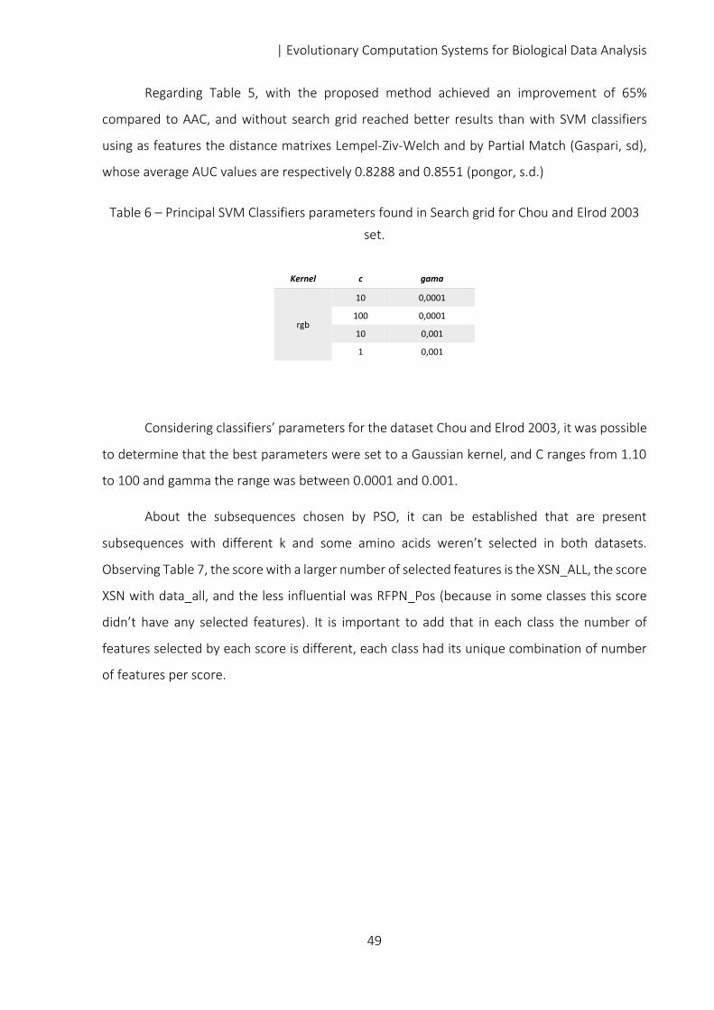
| Evolutionary Computation Systems for Biological Data Analysis
49
Regarding Table 5, with the proposed method achieved an improvement of 65%
compared to AAC, and without search grid reached better results than with SVM classifiers
using as features the distance matrixes Lempel-Ziv-Welch and by Partial Match (Gaspari, sd),
whose average AUC values are respectively 0.8288 and 0.8551 (pongor, s.d.)
Table 6 – Principal SVM Classifiers parameters found in Search grid for Chou and Elrod 2003
set.
Kernel c gama
rgb
10 0,0001
100 0,0001
10 0,001
1 0,001
Considering classifiers’ parameters for the dataset Chou and Elrod 2003, it was possible
to determine that the best parameters were set to a Gaussian kernel, and C ranges from 1.10
to 100 and gamma the range was between 0.0001 and 0.001.
About the subsequences chosen by PSO, it can be established that are present
subsequences with different k and some amino acids weren’t selected in both datasets.
Observing Table 7, the score with a larger number of selected features is the XSN_ALL, the score
XSN with data_all, and the less influential was RFPN_Pos (because in some classes this score
didn’t have any selected features). It is important to add that in each class the number of
features selected by each score is different, each class had its unique combination of number
of features per score.

5|Results
50
Table 7 – The average number of features selected in each score in each class and set for
Chou and Elrod 2003
Scores Average of number features
AFPC_All 5,67
AFPC_Neg 2,67
AFPC_Pos 2,60
AFPN_All 6,20
AFPN_Neg 3,47
AFPN_Pos 3,53
ASFC_All 5,33
ASFC_Neg 2,67
ASFC_Pos 2,27
ASFN_All 5,67
ASFN_Neg 2,93
ASFN_Pos 2,93
FSC_All 5,53
FSN_All 5,07
KFC_All 5,33
KFC_Neg 2,67
KFC_Pos 2,27
KFN_All 5,67
KFN_Neg 2,93
KFN_Pos 2,93
RFPC_Neg 2,13
RFPC_Pos 2,60
RFPN_Neg 3,40
RFPN_Pos 2,00
TFC-idf_All 5,60
TFC-idf_Neg 2,27
TFC-idf_Pos 3,00
TFN-idf_All 5,00
TFN-idf_Neg 3,00
TFN-idf_Pos 2,80
XSC_All 6,00
XSN_All 6,47

| Evolutionary Computation Systems for Biological Data Analysis
51
Table 8 – Estimated running time (hour) for each step method per class.
Data set Scoring Max Scoring PSO PSO with search grid
Scop40mini 50 5 360 600
Chou and Elrod 2003
37 3 200 475
Finally, it should be distinguished in Table 8, the running time required for SCOP40mini
was higher for the Chou and Elrod 2003, and the process with higher execution time was the
PSO with search grid. The estimate was based on files created during the process.

5|Results
52
5|Results

| Evolutionary Computation Systems for Biological Data Analysis
53
6|Discussion In this chapter, it will be discussed the results presented in the previous chapter,
including how the proposed method can be influenced, its effectiveness in predicting proteins’
class families in both datasets, as well as its major limitations.
6.1 |Proposed Method and its Variables
As for the variables that can influence the proposed method, the obtained results are
quite interesting.
Regarding the type of PSO used, PSO-F had better results, meaning in a space of possible
features, they were selected with equal weight to best characterize a class. The PSO-W and
PSO-WF were created on the idea that each score can assign features that can hold different
types of interactions in a protein, and therefore some interactions can be more important than
others. But in the results was expressed that every iteration present in each feature must have
the same weight as the others.
Regarding the type of MaxScoring, MS-WPS led to better results, in which allows to
conclude that the shorter subsequences that are contained in subsequences with higher length
will be ignored, so in most cases the longer subsequence has a score value higher than the
other subsequences but lower than its parent subsequence (shorter sequence).
So for example a subsequence “aaa” and the subsequence “aaaa”, the one with more
amino acids is more important despite the score being smaller, which makes sense because the
more specific a subsequence is, more information as feature has.

6|Discussion
54
As for different values of M, the best value to be used is 10, since with higher M values
can exceed the number of selected features recommended to not occur overfitting. M values
lower than 10 can lead to use PSO on the scores in an insignificant way, because by giving
reduced search spaces within each score, the PSO will be choosing between sequences and not
scores, and what it is desired is selection of the best subsequence in each score obtaining a
multi parameter representation of a protein.
About the types frequently used, when comparing both, FC led to better results, making
possible to conclude that the interactions between consecutive amino acids are more relevant
than those more distant. However, the best results are found when using the FC and the
difference between the two frequencies. For some classes was necessary both frequencies in
particulars features, and this is similar to what happens in some proteins.
Regarding the number of iterations, this increases when there is more information
available, if k or the number of samples in the training set is higher or the search grid is used.
And with more necessary iterations more run time is needed, making the method too time
consuming. However, the need to increase the number of iterations is normal with the increase
of information or more variables present in order to converge to a solution.
These statements are true for most classes but not for all, so it would be interesting to
analyze why, and what dataset characteristics that leads to other types of PSO or frequency.
6.2 |Performance
As can be seen in the results, with the proposed method the average AUC value was
always higher than the value obtained by other methods based on AAC for the two different
data sets. With the proposed method, It was achieved good results regardless of the data set
characteristics, such as the percentage of positives in SCOP40mini which is extremely reduced.
The other methods on an unbalanced data set failed to attain reasonable results (about 0.5
AUC).

| Evolutionary Computation Systems for Biological Data Analysis
55
6.3 |Limitations
Despite the favorable results obtained with the proposed method, there are certain
characteristics that lead to its disadvantage, and one of them is the scoring, it is the first step
and requires a value k. In this work as mentioned above, it was used k equal to 5, which already
leads to the calculation of scores for over 3 million combinations for only one class. This leads
that chosen number k is conditional to the computing power it is available, and the domains
and motifs have more than 5 amino acids.
The biggest limitation is the implementation of the method with the PSO, which needs
high computing power because it is a very time consuming iterative method and uses as fitness
functions the AUC obtained by training new SVM classifiers each iteration. Because of it, the
high M number, or a high number of samples used could lead to a higher running time needed.

6|Discussion
56

| Evolutionary Computation Systems for Biological Data Analysis
57
7|Conclusion In this chapter, it will be discussed the main achievements of this thesis as well as reflect
on the possible applications of this method.
7.1 |Proposed Method
Given the results and their discussion the main objective of this thesis was achieved. It
has created a new method for extraction and selection of features from the primary structure
of a protein that led to better results than many of the methods mentioned, and also it was
successful when applied to two different datasets. Unlike methods based on AAC, this method
continued to show good results with date set with a low percentage of positives.
With this method was accomplished a representation of proteins that takes into
account various aspects and events that other methods so far had not done, also using the AUC
as fitness function and the combination of multiple scores, it was something never done before.
7.2 |Practical Applications
Another positive aspect of this work is that it was not only created a new method, as it
was also created an C # application and a website that make all this research practical and able
to performed by any user, so the method can be applied easily and appropriately. And also, by
having created these tools and making then available it may contribute to validate even better
the proposed method because it allows the user to handle all variables adjacent to the method
and test it in any dataset.

7|Conclusion
58
7.3 |Future Work
Despite the many positive aspects of this thesis, there is still much work to be done so
that the using this method can have a significant impact on several areas of interest (medicine,
pharmaceutical industry, etc.). This is because this method still has some limitations that can
be eliminated.
One of these limitations is the running time of the method. It is crucial to form and plan
different options to significantly reduce this execution time without affecting the method
performance, in order to properly be used as a research pool.
Another limiting aspect is the definition of the number of iterations that the AUC
remains unchanged to stop the iterative PSO, because this is not able to lead to the true
convergence of different particles for the best possible AUC value, since this can be obtained
before or after the number of iterations set.
Furthermore, it is also necessary to validate this proposed method in different biological
data whose structure is also a sequence of coding elements (letters), such as RNA and DNA.
This highlights the advantages in using the proposed method, because it does not require
anything other than a set with samples consisting of a sequence of letters, and it can be used
for different purposes, like the prediction of classes, cell locations, molecular targets, etc.,
depending of the set objective.
Also in the future, after the resolution of the method’s limitations and the search and
storage of different optimized SVM classifiers, this research has the objective of building a
Multiclass classifier to have a structure that predicts what class a protein belongs and not only
if it is part or not of a single set.
In conclusion, all existing sub-sequences in the protein sequence are analyzed by
different statistical importance: by their rarity, size, discriminatory power, independence and
others. Then they are selected according to these different scores, leading to a significant
reduction in the search space as well as a different particle initialization for Particle Swarm
Optimization.
This method primes a different analysis of a protein sequence, along with a minor loss of
information since this analysis is not only supported with one or two factors. By having such

| Evolutionary Computation Systems for Biological Data Analysis
59
promising results this method brings new ideas to improve even a better solution to the problem
in hands.

7|Conclusion
60

| Evolutionary Computation Systems for Biological Data Analysis
61
Appendix
Table 9 - The number and percentage (Rate) of positives in train and test sets for each class
considering the number of negatives in SCOP40mini dataset.
Class Train Set Test Set
Positives Negatives Rate (%) Positives Negatives Rate (%)
1 21 664 3,07 6 666 0,89
2 18 661 2,65 17 661 2,51
3 38 656 5,48 6 657 0,90
4 23 656 3,39 21 657 3,10
5 39 652 5,64 12 654 1,80
6 46 652 6,59 5 654 0,76
7 42 652 6,05 9 654 1,36
8 92 628 12,78 9 628 1,41
9 100 615 13,99 25 617 3,89
10 117 615 15,98 8 617 1,28
11 73 615 10,61 52 617 7,77
12 34 652 4,96 18 653 2,68
13 43 654 6,17 5 655 0,76
14 43 654 6,17 5 655 0,76
15 42 654 6,03 6 655 0,91
16 41 654 5,90 7 655 1,06
17 51 642 7,36 20 644 3,01
18 66 642 9,32 5 644 0,77
19 47 642 6,82 24 644 3,59
20 66 642 9,32 5 644 0,77
21 27 660 3,93 10 660 1,49
22 34 656 4,93 10 657 1,50
23 18 656 2,67 26 657 3,81
24 53 639 7,66 25 640 3,76
25 65 639 9,23 13 640 1,99
26 10 670 1,47 6 671 0,89
27 103 604 14,57 46 604 7,08
28 124 604 17,03 25 604 3,97
29 140 604 18,82 9 604 1,47
30 137 604 18,49 12 604 1,95
31 134 604 18,16 15 604 2,42
32 134 604 18,16 15 604 2,42
33 16 667 2,34 5 669 0,74
34 11 668 1,62 8 670 1,18
35 51 650 7,28 5 651 0,76
36 25 650 3,70 31 651 4,55

Appendix
62
37 161 592 21,38 12 592 1,99
38 159 592 21,17 14 592 2,31
39 159 592 21,17 14 592 2,31
40 155 592 20,75 18 592 2,95
41 151 592 20,32 22 592 3,58
42 166 592 21,90 7 592 1,17
43 168 592 22,11 5 592 0,84
44 142 592 19,35 31 592 4,98
45 166 592 21,90 7 592 1,17
46 53 644 7,60 16 644 2,42
47 55 644 7,87 14 644 2,13
48 63 644 8,91 6 644 0,92
49 53 644 7,60 16 644 2,42
50 19 663 2,79 11 664 1,63
51 32 654 4,66 16 655 2,38
52 34 654 4,94 14 655 2,09
53 13 668 1,91 7 669 1,04
54 13 667 1,91 10 667 1,48
55 15 668 2,20 5 669 0,74
Average 70,93 635,62 9,80 14,02 636,44 2,15
| Evolutionary Computation Systems for Biological Data Analysis
63
References A, H. et al., 2006. Significantly improved prediction of subcellular localization by integrating text
and protein sequence data. Pacific Symposium on Biocomputing. Pacific Symposium on
Biocomputing, pp. 16-27.
Annette Hoglund, P. D. T. B. H.-W. A. K., 2006. MultiLoc: prediction of protein subcellular
localization using N-terminal targeting sequences, sequence motifs and amino acid
composition, Oliver Kohlbacher. Bioinformatics, Volume 22, pp. 1158-1165.
Bagyamathi, M. & Inbarani, H. H., 2015. A Novel Hybridized Rough Set and Improved Harmony
Search Based Feature Selection for Protein Sequence Classification. Big Data in Complex
Systems, Volume 9, pp. 173-204.
Bin Liu, J. C. X. W., 2015. Protein remote homology detection by combining Chou’s distance-pair
pseudo amino acid composition and principal component analysis. Mol Genet Genomics , pp.
1919-1931.
biofor, s.d. Amino Acid's Mass List. [Online]
Available at: http://www.bioinfor.com/peaks/downloads/masstable.html
Campbell, N., 1996. Biology. Fourth edition ed. The Benjamin/Cummings Publishing Company:
The Benjamin.
Chieh-Yuan Tsai, C.-J. C., 2014. A PSO-AB classifier for solving sequence classification problems.
Chou, K.-C., 2001. Prediction of Protein Cellular Attributes Using PseudoAmino Acid
Composition. PROTEINS: Structure, Function, and Genetics, Volume 43, p. 246–255.
Chou, K.-C., 2004. Using amphiphilic pseudo amino acid composition to predict enzyme
subfmily classes. BioInformatics vol 21 issue 1, pp. 10-19.
Chou, K.-C. & Elrod, D. W., 2003. Prediction of Enzyme Family Classes. Journal of Proteome
Research, pp. 183-190.
C, T., 1962. Contribution of hydrphobic interactions to the stability. J Am Chem Soc, Volume 84,
p. 4240–4274.

References
64
developers, s.-l., s.d. scikit-learn Machine Learning in Python. [Online]
Available at: http://scikit-learn.org/stable/
Fisher, R. A., 1936. The use of multiple measurements in taxonomic problems. Annals of
Eugenics, Volume 7, p. 179–188.
Guda, A. M. a. C., 2011. Computational Approaches for Automated Classification of Enzyme
Sequences. J Proteomics Bioinform, pp. 147-152.
Hoglund, A. et al., 2005. Using N-terminal targeting sequences, amino acid composition, and
sequence motifs for predicting protein subcellular localization. Proceedings of the German
Conference on Bioinformatics, pp. 45-49.
Hopp TP, W. K., 1981. Prediction of protein antigenic determinants. Proc Natl Acad Sci USA,
Volume 78, p. 3824–3828.
Huang, Q.-Y., You, Z.-H., Li, S. & Zhu, Z., 2014. Using Chou's amphiphilic Pseudo-Amino Acid
Composition and Extreme Learning Machine for prediction of Protein-protein interactions.
International Joint Conference on Neural Networks (IJCNN).
Kashif Ishaque, Z. S., 2012. An Improved Particle Swarm Optimization (PSO)–Based MPPT for
PV With Reduced Steady-State Oscillation. IEEE Transactions on Power Electronics, Volume 27.
kegg, s.d. Amino Acid List. [Online]
Available at: http://www.genome.jp/kegg/catalog/codes1.html
Kennedy, J. & Eberhart, R., 1995. Particle Swarm Optimization. Proceedings of IEEE International
Conference on Neural Networks.
Liu, B. et al., 2015. repRNA: a web server for generating various features vectores of RNA
sequences. Mol Genet Genomics , p. 473–481.
Liu, B. et al., 2015. Pse-in-One: a web server for generating various modes of pseudo
components of DNA, RNA, and protein sequences. Nucleic Acids Research, Volume 43, pp. W65-
W71.

| Evolutionary Computation Systems for Biological Data Analysis
65
Mandal, M., Mukhopadhyay, A. & Maulik, U., 2015. Prediction of protein subcellular localization
by incorporating multiobjective PSO-based feature subset selection into the general form of
Chou’s PseAAC. Medical & Biological Engineering & Computing, Volume 53, p. 331–344.
Mohabatkar, H., Mohammad , M. B., Abdolahi, K. & Mohsenzadeh, S., 2013. Prediction of
Allergenic Proteins by Means of the Concept of Chou's Pseudo Amino Acid Composition and a
Machine Learning Approach. Medicinal Chemistry, pp. 133-137.
Nishikawa, K., Kubota, Y. & OOI, T., 1983. Classification of Proteins into Groups Based on Amino
Acid Composition and Other Caracter.. J.Biochem, pp. 981-985.
OpenPyxl, s.d. OpenPyxl. [Online]
Available at: https://openpyxl.readthedocs.io/en/default/
Paolo Sonego, M. P. S. D. A. K.-F. A. K. Z. G. J. A. L. a. S. P., 2006. A Protein Classification
Benchmark collection for machine learning. Nucleic Acids Research, p. D232–D236..
Pedersen, Y. Y. a. J. O., 1997. A comparative study on feature selection in text categorization.
Proceedings of International Conference on Machine Learning, p. 412–420.
Petsko, G. A. & Ringe, D., 2004. Protein Structure and Function. s.l.:Blackwell Publishing.
Sahu, S. S. & Panda, G., 2010. A novel feature representation method based on Chou’s pseudo
amino acid composition for protein structural class predictio. Computational Biology and
Chemistry 34, p. 320–327.
Shena, H. & Choua, K.-C., 2005. Using optimized evidence-theoretic K-nearest neighbor
classifier and pseudo-amino acid composition to predict membrane protein types. Biochemical
and Biophysical Research Communications, Volume 334, pp. 288-292.
Tian, W. & Skolnick, J., 2003. How Well is Enzyme Function Conserved as a Function of Pairwise
Sequence Identity?. Journal of Molecular Biology, Volume 333, p. 863–882.
Tsaia, C.-Y. & Chena, C.-J., 2015. A PSO-AB classifie for solving sequence classification problems.
Applied Soft Computing, Volume 27, pp. 11-27.
Wen-Yun Yang, B.-L. L. a. Y. Y., 2006. A Comparative Study on Feature Extraction from Protein
Sequences for Subcellular Localization Prediction.

References
66
Wu, Y., Tang, H., Chen, W. & Lin, H., 2016. Predicting Human Enzyme Family Classes by Using
Pseudo Amino Acid Composition. Current Proteomics, pp. 99-104.
Xu, Y., Ding, J., Wu, L.-Y. & Chou, K.-C., 2013. iSNO-PseAAC: Predict Cysteine S-Nitrosylation
Sites in Proteins by Incorporating Position Specific Amino Acid Propensity into Pseudo Amino
Acid Composition. PLoS One.
Yang, W.-Y., Lu, B.-L. & Yang, Y., 2006. A Comparative Study on Feature Extraction from Protein
Sequences for Subcellular Localization Prediction. Proceedings of the 2006 IEEE Symposium on
Computational Intelligence in Bioinformatics and Computational Biology, pp. 201-208.
Yang, W.-Y., Lu, B.-L. & Yang, Y., 2006. A Comparative Study on Feature Extraction from Protein
Sequences for Subcellular Localization Prediction. IEEE Symposium on Computational
Intelligence and Bioinformatics and Computational Biology, pp. 201-208,.
Yang, Y., 2011. A Comparative Study on Sequence Feature Extraction for Type III Secreted
Effector Prediction. 2011 Eighth International Conference on Fuzzy Systems and Knowledge
Discovery (FSKD), pp. 1560-1564.
Yiming Yang, J. O. P., 1997. A Comparative Study on Feature Selection in Text Categorization.
ICML '97 Proceedings of the Fourteenth International Conference on Machine Learning, pp. 421-
420.
Zhou, G.-P. & Doctor, K., 2003. Subcellular Location Prediction of Apoptosis Proteins. Proteins:
Structure, Function, and Genetics 50, pp. 44-48.
Zhou, X.-B., Chen, C., Li, Z.-C. & Zou, X.-Y., 2007. Using Chou's amphiphilic pseudo-amino acid
composition and support vector machine for prediction of enzyme subfamily classes.. Journal
of Theoretical Biology, Volume 248, pp. 546-551.
