Religion and Education: Evidence from the National Child Development Study

Sarah Brown and Karl Taylor*

Department of Economics University of Leicester

University Road, Leicester Leicestershire LE1 7RH

England

Abstract: In this paper, we explore the determinants of one aspect of religious behaviour – church attendance – at the individual level using British data derived from the National Child Development Study (NCDS). To be specific, we focus on the relationship between education and church attendance, which has attracted some attention in the existing literature. In contrast to the previous literature in this area, our data allows us to explore the dynamic dimension to religious activity since the NCDS provides information on church attendance at three stages of an individual’s life cycle. The findings from our cross-section and panel data analysis, which treats education as an endogenous variable, support a positive association between education and church attendance. In addition, our findings suggest that current participation in religious activities is positively associated with past religious activities. Furthermore, our findings suggest that levels of religious activity tend to vary less over time suggesting that factors such as habit formation may be important.

Key Words: Church Attendance; Education; Human Capital; Religion. JEL Classification: J24, Z12

Acknowledgements: We are grateful to the Data Archive at the University of Essex for supplying the National Child Development Study, waves 1 to 6. The normal disclaimer applies.

*Corresponding author Dr Karl Taylor, email kbt3@le.ac.uk or Tel: +44 (0)116 252 5368.

November 2003

2

I. Introduction

Religious activity is one area of household behaviour that has attracted very little interest in

the economics literature [Sawkins et al. (1997)]. Although the boundaries surrounding areas

of economics have been widened, there has appeared to be some reluctance amongst

economists to incorporate religion, although it has been argued that economic frameworks

may provide the best contexts in which to model religious behaviour [Stark et al. (1996)].

Such reluctance is surprising since as argued by Iannaccone (1998):

Studies of religion promise to enhance economics at several levels: generating information about a neglected area of “nonmarket” behavior; showing how economic models can be modified to address questions about belief, norms and values; and exploring how religion affects economic attitudes and activities of individuals, groups and societies. [Iannaccone (1998), p.1465].

Over the last decade or so, there has been a mild flurry of interest into this expanding area of

economics with most of the empirical work based on U.S. data [see Iannaccone (1998) for an

excellent survey of the economics of religion]. One strand of the literature has employed

microeconomic theory to explore the determinants of religious behaviour such as the decision

to participate in religious activities – a decision that may vary over an individual’s life cycle

[Smith et al. (1998)].

The aim of this paper is to explore the determinants of one measure of religious

activity – church attendance – at the individual level using British panel data derived from the

National Child Development Study (NCDS). Moreover, we focus on one specific

characteristic of individuals, which has been the subject of much scrutiny by economists over

many decades – namely education. Iannaccone (1998) outlines a number of interesting

questions, which have been raised concerning the relationship between religion and education

in the context of secularisation. For example, is it the case that individuals become less

religious and more sceptical of faith-based claims as they acquire more education? Is this

3

more pronounced as individuals acquire more education in the sciences? Many studies have,

however, reported that rates of religious activity such as church attendance in fact increase

with education.

Despite the fact that many studies report a positive association between education and

religious activity, as pointed out by Sander (2002) such findings do not mean that education

actually increases religious activity. In general, the existing studies in this area have treated

education as exogenous despite the early work by Azzi and Ehrenberg (1975) who argue that

human capital variables should be treated as endogenous. Sander (2002) expands the existing

research in this area by treating education as an endogenous variable and finds that there is no

causal affect of education on religious activity using U.S. cross-section data.

In this paper, we build upon the approach of Sander (2002) in three main ways.

Firstly, we expand the church attendance equation to incorporate a richer array of explanatory

variables. Secondly, we drawn upon the recent economics of education literature and specify a

more comprehensive educational attainment equation in order to control for endogeneity bias.

Furthermore, in contrast to Sander (2002) who analyses years of education, we are able to

explore an additional and perhaps preferable measure of educational attainment – namely –

highest educational qualification obtained. Thirdly, we analyse individual panel data thereby

enabling us to explore religious activity from a dynamic perspective, i.e. at different points of

an individual’s life cycle.

The findings from our cross-section and panel data analysis support a positive

association between education and church attendance. In addition, our findings suggest that

current participation in religious activities is positively associated with past religious

activities. Furthermore, our findings suggest that levels of religious activity tend to vary less

over time suggesting that factors such as habit formation may be important. To summarise,

our results suggest that a time dimension to religious activity exists. Furthermore, the

4

importance of previous religious activity in determining current levels of religious activity

suggests that omitting such factors from econometric analysis may lead to biased results and

erroneous inferences.

The rest of the paper is set out as follows. Section II discusses the background issues

surrounding the relationship between religion and education. Section III describes the data

and methodology employed. Section IV presents the results of our empirical analysis whilst

our concluding comments are collected in Section IV.

II. Background

In general, economists have explored the decision to engage in religious activity from the

perspective of a time allocation model. Azzi and Ehrenberg (1975), for example, explored

church attendance in the U.S. in the context of a household allocation of time model where

participation in religious activity served to raise consumption in the ‘afterlife.’ This seminal

contribution to the area has been modified and extended in a number of ways. One

modification, for example, entails allowing religious activity to enhance current as well as

‘afterlife’ utility [see Iannaccone (1998)]. One of the key implications drawn from such a

framework is that the time allocated to religious activity may initially fall then rise with age

given that the opportunity cost of religious activity is initially high at the start of an

individual’s career when faced with a relatively steep age-earnings profile. As age increases,

however, the age-earnings profile typically flattens thereby reducing the opportunity cost

associated with religious activity [Sawkins et al. (1997)].

Thus, empirical studies have included a combination of personal characteristics such

as age and labour market characteristics for example earnings as explanatory variables in

regression models seeking to explain levels of religious activity such as church attendance. In

general, cross-section data has been employed to explore religious activity. It is apparent,

5

however, as indicated above that the time dimension plays an important role in the context of

time allocation models with the costs of particular activities being sensitive to the stages of an

individual’s life cycle. Hence, the analysis of panel data would clearly be preferable in this

context. However, the findings from the cross-section studies do provide some interesting

insights into the determinants of religious activity at a given point in time.

Educational attainment plays an important role in determining the opportunity cost of

engaging in activities such as religion. As argued by Brañas Garza and Neuman (2003), the

predicted effect of schooling on religious activities is, however, somewhat ambiguous. If the

opportunity cost of time devoted to religious activities is positively related to education, then

one would predict an inverse relationship between religious activities and educational

attainment. Furthermore, as outlined above, individuals may become less religious as

education increases as they become more inclined to reject faith-based beliefs. Sacerdote and

Glaeser (2002), however, argue that if education increases the returns from social activities,

then one might predict a positive association between education and religious activities (i.e. a

formal social activity). Barro and McCleary (2002) propose an alternative explanation for the

positive association between religious activity and education – given that religious beliefs

entail a degree of abstraction and that more educated individuals are relatively capable of

scientific and abstract thought, they might be able to rationalise religious beliefs in this way.

Thus, given that the predicted effect of schooling on religious activities is somewhat

ambiguous, empirical analysis is required to shed some light in this area. The empirical work

in this area has predominantly used U.S. data. In general, church attendance has been found to

be positively associated with educational attainment [see, for example, Iannaccone (1998) and

Sacerdote and Glaeser (2002)]. Furthermore, Sacerdote and Glaeser (2002) state:

‘In many multivariate regressions, education is the most statistically important factor explaining church attendance.’ [Sacerdote and Glaeser (2002), p.2].

6

Sacerdote and Glaeser (2002) explore an interesting puzzle related to religious attendance in

the U.S. where religious attendance increases sharply with education across individuals yet

declines sharply with education across denominations with the more highly educated

denominations being characterised by the lowest rates of church attendance. The key to

explaining this puzzle lies in the existence of omitted variables, which differ across

denominations. Furthermore, Sacerdote and Glaeser argue that the most likely omitted

variable is the degree of religious beliefs and they provide evidence that measures of religious

beliefs are strongly correlated with church attendance yet negatively correlated with education

for a number of countries including the U.S. and Great Britain. Moreover, they provide some

evidence of a causal link that education moderates religious beliefs. They also provide

evidence supporting the hypothesis that the positive association between education and

church attendance is due to omitted variables related to social skills and propensity to engage

in formal social activities. The reasoning behind this is that schooling and church attendance

are both formal social group activities – hence we would predict a positive correlation

between the two activities.

Sacerdote and Glaeser provide cross-section evidence for the U.S. and throughout the

world, indicating that education is positively associated with all forms of social behaviour,

that religious attendance is correlated with other forms of social activity and that schooling is

not correlated with non-social religious behaviour. In sum, according to these hypotheses,

more educated individuals are more likely to attend church (i.e. to engage in this formal social

activity) but are less likely to accept, for example, the literal truth of the bible. Sacerdote and

Glaeser compare their U.S. findings based on the U.S. General Social Survey, across

countries by analysing the World Values Survey. They find a positive relationship between

education and church attendance at the individual level in Great Britain, Spain, Sweden and

7

France, a negative relationship in other countries including Poland and Russia and a

statistically insignificant relationship in a number of other countries.

Sawkins et al. (1997), one of the rare studies focusing on British data, find that church

attendance is positively correlated with educational attainment when attendance equations are

estimated separately for males and females using cross-section data derived from the first

wave of the British Household Panel Survey. Similarly, Brañas Garza and Neuman (2003)

who explore the level of religiosity as measured by beliefs, prayer and church attendance

amongst Spanish Catholics by estimating separate equations for males and females, report a

marginally significant positive relationship between schooling and religiosity. One of the

important features of this study is that the data allows the authors to distinguish between

private and public religious activity. To be specific, the positive relationship is statistically

significant for women for both participation in mass (i.e. a public activity) and prayer (i.e. the

private activity) yet only significant for men in the case of participation in mass.

Although a number of studies report a positive association between education and

religious activity,1 as pointed out by Sander (2002) these findings do not necessarily mean

that education is positively related to religious activity. In general, such studies have treated

education as exogenous despite the early work by Azzi and Ehrenberg (1975) who argue that

human capital variables should be treated as endogenous. Sander expands the existing

research in this area by treating education as an endogenous variable and finds that there is no

causal affect of education on religious activity using U.S. cross-section data.2

In the following section, we introduce the data and the empirical methodology

employed to assess the impact, if any, educational attainment has on religious attendance in

1 Neuman (1986) is one exception in the literature who reports an inverse relationship between schooling and time spent on religious activities among Jewish males in Israel. One of the defining features of this study is that unlike the majority of studies in this area, which rely on an index of church attendance, religiosity is measured by the total number of hours spent on religious activities. 2 The over-identifying instruments for the education equation used in Sander’s analysis are parent’s schooling.

8

Great Britain. An advantage of our approach is that our data enables us to control for potential

endogeneity effects, as highlighted by Azzi and Ehrenberg (1975) and Sander (2002), within a

panel framework and, thus, to focus on an area unexplored in the literature to date, namely the

dynamics of religious attendance.

III. Data and Methodology

Our empirical analysis is based on the British National Child Development Study (NCDS)

which is a panel survey following a cohort of children born during a given week (March 3rd to

March 9th) in 1958. This panel study provides a wealth of information relating to family

background in addition to the advantages of tracing an individual over a relatively long time

horizon. The Survey was conducted at ages 7, 11, 16, 23, 33 and 42.

The NCDS is particularly appropriate for our analysis since it provides information

pertaining to church attendance in addition to detailed information relating to educational

attainment. In terms of church attendance, respondents were asked the following question at

three points during their life cycle – at ages 23, 33 and 42:

How often, if at all, do you attend services or meetings connected with your religion?

‘never or very rarely’ 0

‘sometimes, but less than once a month’ 1

‘once a month or more’ 2

‘once a week’ 3

We use the information to construct a 4-point church attendance index, providing information

about the level of church attendance at three points in time.3 We conduct two types of analysis

(i) cross-section analysis for the latest survey conducted at age 42 where the dependant

variable is given by the church attendance index in 2000, ir , and (ii) panel data analysis

3 It is important to acknowledge that our index of church attendance is a proxy for time spent in religious activities. Time spent on other religious activities such as praying is clearly omitted from our dependent variable.

9

where we pool the information for individuals across the three time periods (1981, 1991 and

2000) in order to explore how church attendance, itr , varies over an individual’s life cycle.

Cross-Section Analysis

Given the nature of the dependent variable we initially specify an ordered probit model:

10 iii*i er Xφ

' (1)

where *ir is the unobservable propensity of individual i to attend church; ir is the

individual’s observed church attendance; ie denotes the educational attainment of individual

i and iX denotes a vector of personal and demographic characteristics.4 In order to explore

the dynamic dimension to the church attendance decision, we include two lagged dependent

variables – one denoting church attendance at age 33 and the other denoting church

attendance at age 23. Our cross-section data set pertaining to 2000, i.e. age 42, comprises

6,913 individuals.

Turning to the explanatory variables, educational attainment can be measured via a

variety of approaches. We compare two commonly used measures – namely years of

education and highest educational qualification obtained. In the initial analysis, we specify

educational attainment as an exogenous explanatory variable in the religious activity equation.

Following Sander (2002), we then allow for the possibility that educational attainment may be

endogenous with respect to religious activity. Thus, we incorporate an educational attainment

equation into our empirical analysis and replace ie with its predicted value, ie as follows:

iii fe Z (2a)

10 iii*i er Xφ

' (2b)

4 In an ordered probit model, the probability that the observed outcome j (there are 4 outcomes, see above) is in

the range of the estimated cut-off points, j , is given by jiiiji

eprjrpr Xφ'

101 .

10

In order to create the predicted values of education, the functional form of Equation 2a differs

according to our definition of educational attainment. In the case of years of education, we

adopt a standard OLS approach whilst in the case of highest educational qualification

obtained, we follow Dearden et al. (2002) by adopting an ordered probit model given that

educational attainment can be described by a single index.5 Our highest educational

attainment index is defined on a 7-point scale with zero representing no educational

qualifications, 1 denotes CSE level education (a relatively ‘low’ school qualification taken at

age 16), 2 denotes O level (a relatively ‘high’ school qualification taken at age 16), 3 denotes

A level (the school qualification taken at age 18), 4 denotes diploma (i.e. intermediate

qualifications between high school and university degree), 5 denotes degree (i.e. a Bachelors

degree) and 6 denotes a higher degree (i.e. a Masters degree or a PhD).

There has been much recent interest in the economics literature and amongst policy-

makers into the determinants of educational success with attention being paid to the

relationship between school quality and academic performance. Thus, we draw upon this

literature in order to specify our educational attainment equation, Equation 2a. The

explanatory variables, given in iZ , are divided into three groups; school quality, family

background and ability and largely build upon the specifications of Dearden et al. (2002) and

Dustmann et al. (2003).

We adopt one of the standard measures of school quality – the number of pupils per

teacher in the school at both the primary (i.e. pre age 11) and secondary (i.e. post age 11)

stages of education. We also include dummy variables to control for whether, at the age of

16, the individual attends a secondary modern school, a technical school, a comprehensive

school (i.e. non selective and state run), a grammar school (higher ability and state run) or a

private school. We also control for whether the individual attended a single sex school at age

5 Heckman and Cameron (1998) analyse the validity of such an approach.

11

16. Controls also include a dummy variable denoting the presence of a parents-teachers

association as well as a set of dummy variables indicating whether the school lacks library,

sports or other facilities – factors excluded by Deardon et al. (2002) but which arguably could

impinge upon educational attainment.

Family background has been found to be an important determinant of educational

attainment [see Ermisch and Francesconi (2001)]. We incorporate a variety of controls for

family background given that it may influence educational attainment through a number of

different channels – for example through time inputs or financial resources. Family

background variables include parents’ occupation, years of education of parents and

household income. The number of older siblings and the number of younger siblings are

incorporated to explore the argument of Becker (1981) that parental attention declines as

family size increases and to also explore the hypothesis that birth order is important. We also

include information indicating whether the teacher considers the mother and/or father to be

interested in the child’s education at the age of 16. In order to further proxy for family

resources, we include a dummy variable indicating whether the individual has a private room

for studying at age 16. We also include dummy variables indicating whether the child

received free school meals at ages 11 and 16. In addition to controlling for whether the

families experienced financial difficulties, we augment the approach adopted by Dearden et

al. (2002) by also controlling for other difficulties faced by the families such as alcoholism in

the family, death of mother or father and divorce.

In order to proxy ability, we include the individuals’ scores attained in reading and

mathematics tests at ages 7, 11 and 16. We are also able to proxy the child’s attitude towards

school, by including a dummy variable which equals one if he/she was truant at least once

when aged 16.

12

Returning to the religious attendance equation (Equation 2b) and the explanatory

variables in the iX vector, we include a number of controls in addition to education in our

church attendance equation. These include religious denomination, gender, being disabled,

marital status, household size (including presence of pre-school and other children) and

ethnicity.6 One serious omission from our data set relates to information pertaining to parents’

religion and religious upbringing. In order to control for the stock of religious human capital

as a child, we are, however, able to incorporate a dummy variable indicating whether the

individual has a CSE, O level or A level in Religious Education. In order to explore the

arguments put forward by Barro and McCleary (2002), we also incorporate a dummy variable

indicating whether the individual has a CSE, O level or A level qualification in a science

subject.

A set of variables related to economic status is incorporated in the specification

including total income and total income squared (this includes labour and non labour income).

Hence, we explore the argument discussed by Iannaccone (1998) that the opportunity cost of

church attendance increases with income. Controls for labour market status are included by

incorporating dummy variables for unemployment and self-employment as well as whether

the individual’s spouse is unemployed. We follow Ellison (1993) in incorporating measures

of health and life satisfaction to explore the argument that higher rates of religious activity are

associated with increased life satisfaction, improved health and reduced stress. We also

include a dummy variable, which indicates whether the individual feels that he/she has

someone to turn to for support. An index denoting how close the individual feels that the

members of the household are is also added to the model. Following Sacerdote and Glaeser

(2002), we include two variables representing the extent of participation in other formal social

6 Note that age is excluded from the empirical specification since all individuals are of equal age.

13

group activities such as attendance at political party meetings, charity and voluntary group

meetings and attendance at women’s groups.

In order to explore the effects of past religious activity on current religious activity,

we include two lagged dependent variables – one denoting church attendance at age 33 and

the other denoting church attendance at age 23. Past religious activities may be positively

associated with current religious activities since according to Smith et al. (1998):

‘…religious human capital and participation are complements since past and present consumption will be positively related. Moreover, the accumulation of religious human capital provides an incentive for further religious participation, which in turn augments that capital stock. This complementarity generates the habitual character of church attendance.’[Smith et al. (1998), p.29].

Thus, according to such arguments, the dynamic aspect to participation in religious activities

is influenced by the accumulation of experience in religious activities such as knowledge and

understanding of certain rituals or familiarity with hymns and prayers. In other words, the

higher the levels of human capital acquired by participation in religious activities in the past,

the more likely is an individual to continue to engage in religious activities. This is an

important expansion of the current literature which has explored the relationship between

individual religious attendance and education using cross-section data and, thus, has not

focused on the dynamic dimension to religious activity [see, for example, Sawkins et al.

(1997), Iannaccone (1998), Glaeser and Sacerdote (2002), and Sander (2002)].

Panel Data Analysis

Given that the NCDS provides information relating to church attendance at three points of an

individual’s life cycle, we are able to construct a panel of data at the individual level. In

general, the existing studies in this area exploit cross-section data and are, thus, unable to

analyse how an individual’s religious activity varies over his/her life cycle. We explore a

balanced panel of data, which comprises of those individuals who participated in all three

surveys at ages 23, 33 and 42. We have 6,834 individuals who participated in all three surveys

14

yielding a total of 20,502 observations. Given the nature of the dependant variable, we adopt a

random effects ordered probit estimator.

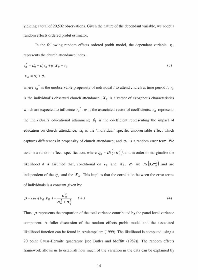
In the following random effects ordered probit model, the dependant variable, itr ,

represents the church attendance index:

10 ititit*it er Xφ

' (3)

itiit

where *itr is the unobservable propensity of individual i to attend church at time period t; itr

is the individual’s observed church attendance; itX is a vector of exogenous characteristics

which are expected to influence *itr ; φ is the associated vector of coefficients; ite represents

the individual’s educational attainment; 1 is the coefficient representing the impact of

education on church attendance; i is the ‘individual’ specific unobservable effect which

captures differences in propensity of church attendance; and it is a random error term. We

assume a random effects specification, where 20, iit IN~ , and in order to marginalise the

likelihood it is assumed that, conditional on ite and itX , i are 20,IN and are

independent of the it and the itX . This implies that the correlation between the error terms

of individuals is a constant given by:

22

2

kl),(corr ikil (4)

Thus, represents the proportion of the total variance contributed by the panel level variance

component. A fuller discussion of the random effects probit model and the associated

likelihood function can be found in Arulampalam (1999). The likelihood is computed using a

20 point Gauss-Hermite quadrature [see Butler and Moffitt (1982)]. The random effects

framework allows us to establish how much of the variation in the data can be explained by

15

unobservable intra-individual correlations. Thus, the magnitude of provides information

pertaining to whether individuals are likely to report consistent levels of religious activity

across the three time periods, conditional upon the underlying covariates, or whether religious

activity is subject to much change over the individual’s life cycle. The analysis of panel data

is particularly appropriate for exploring rates of religious behaviour since age has been found

to be a particularly strong indicator of religious activity with religious activity increasing with

age [see, for example, Iannaccone (1998), Sander (2002) and Sawkins et al (1998)]. Such

findings may be explained by habit formation and/or the importance of afterlife expectations

over time.

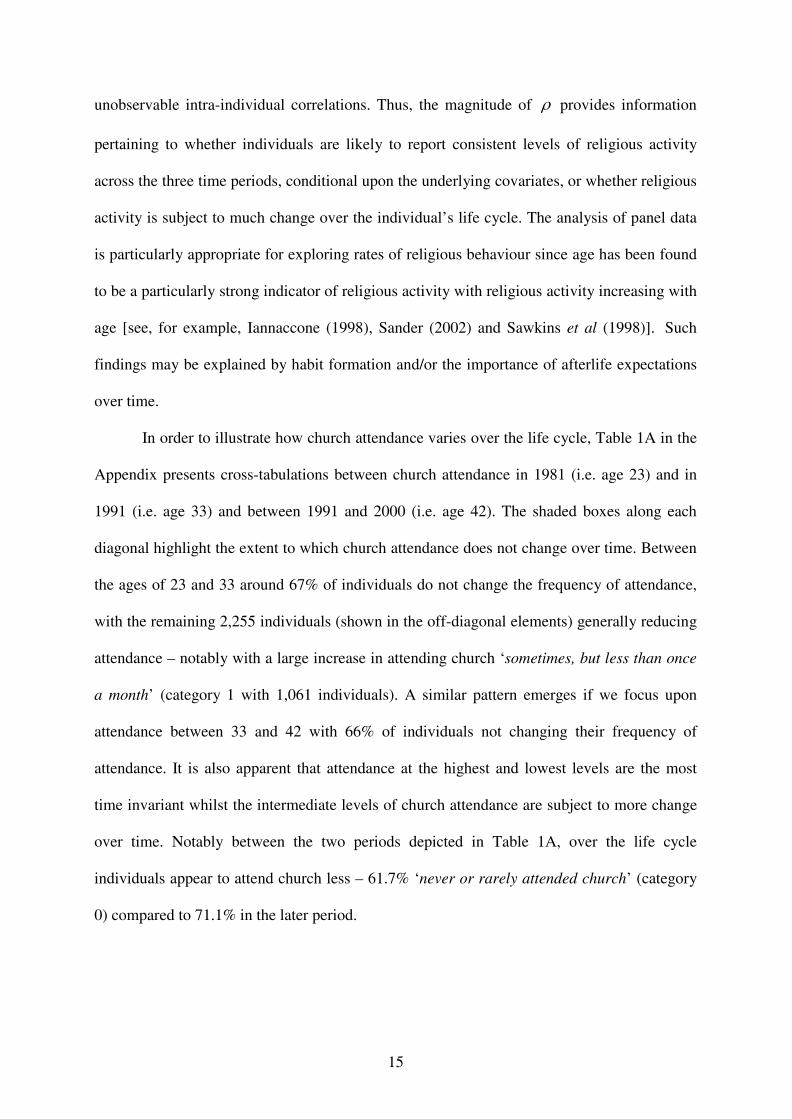
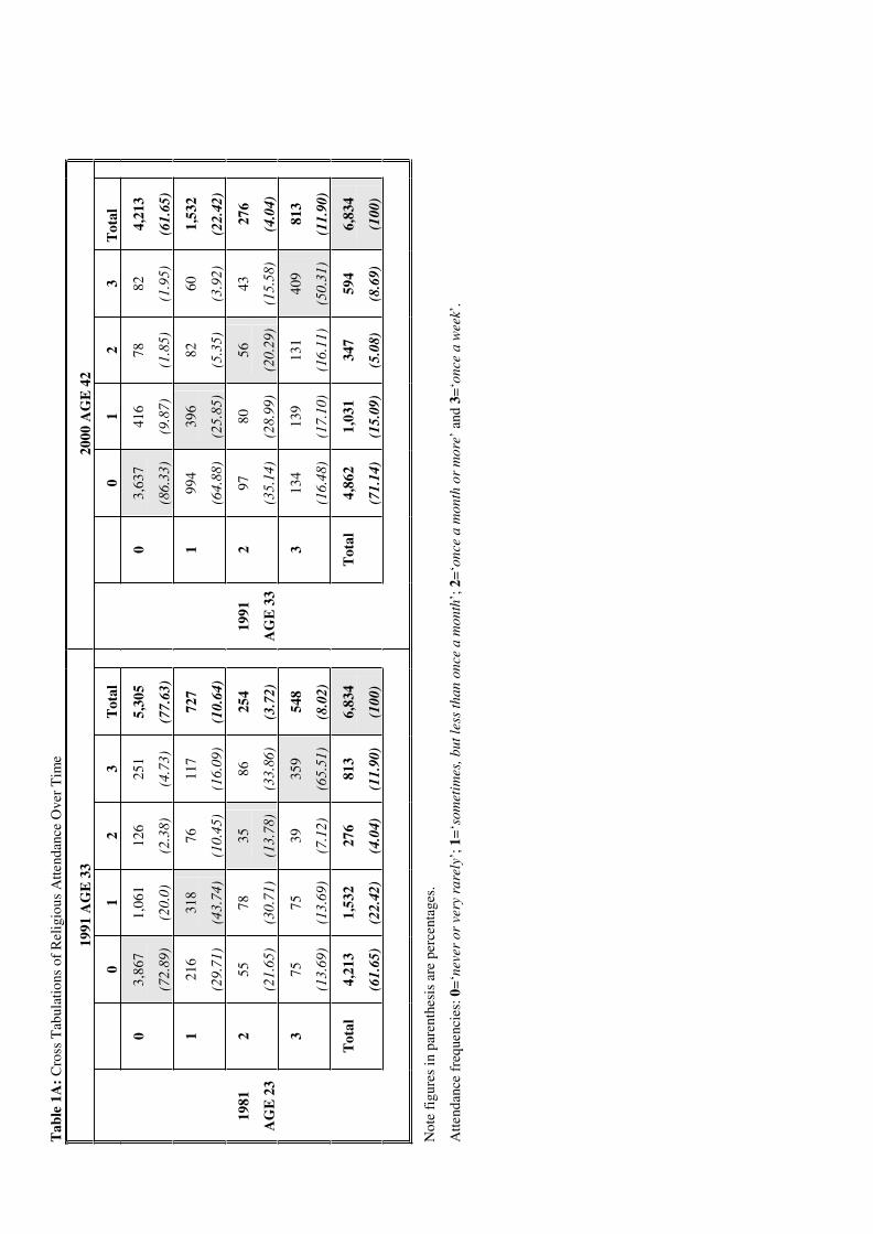
In order to illustrate how church attendance varies over the life cycle, Table 1A in the

Appendix presents cross-tabulations between church attendance in 1981 (i.e. age 23) and in

1991 (i.e. age 33) and between 1991 and 2000 (i.e. age 42). The shaded boxes along each

diagonal highlight the extent to which church attendance does not change over time. Between

the ages of 23 and 33 around 67% of individuals do not change the frequency of attendance,

with the remaining 2,255 individuals (shown in the off-diagonal elements) generally reducing

attendance – notably with a large increase in attending church ‘sometimes, but less than once

a month’ (category 1 with 1,061 individuals). A similar pattern emerges if we focus upon

attendance between 33 and 42 with 66% of individuals not changing their frequency of

attendance. It is also apparent that attendance at the highest and lowest levels are the most

time invariant whilst the intermediate levels of church attendance are subject to more change

over time. Notably between the two periods depicted in Table 1A, over the life cycle

individuals appear to attend church less – 61.7% ‘never or rarely attended church’ (category

0) compared to 71.1% in the later period.

16

We also explore the possibility that education may be endogenous in the context of

our panel data analysis. Hence, we estimate the following:7

ititit ge Z (5a)

10 ititit*it er Xφ

' (5b)

The set of explanatory variables in itX is similar to that used in the cross-section analysis

comprising of a mixture of time varying variables (such as marital status and economic

activity) and time invariant information (such as ethnicity). It is also apparent that the

religious denomination dummies may change over time as individuals switch in and out of

different religions. Iannaccone (1998) argues that we would expect to see the extent of such

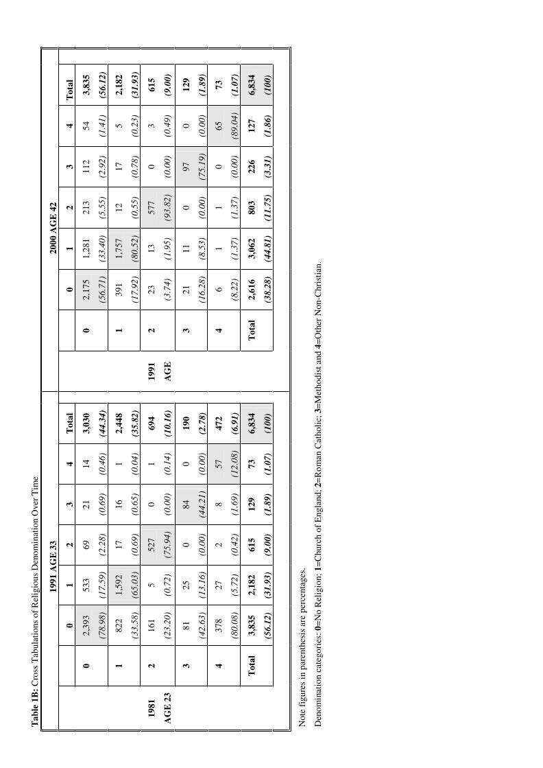
switching to decline over an individual’s lifetime.8 Table 1B in the Appendix presents cross-

tabulations between religious denomination in 1981 (i.e. age 23) and in 1991 (i.e. age 33) and

between 1991 and 2000 (i.e. age 42), thus giving an insight into the dynamics of religious

denomination. The shaded boxes along each diagonal highlight the extent to which religious

denomination does not change over time. For example, between the ages of 23 and 33

approximately 65% of individuals are Church of England (category 1 with 1,592 individuals).

Interestingly there is some variation over time, but as Iannaccone (1998) argued such

switching between denominations does fall over time. This is evident if we focus upon each

denomination between the ages of 33 and 42 where it is apparent that each figure along the

lead diagonal is greater than the counter-part for earlier in the life cycle i.e. aged 23 and 33.

The following section presents the results of the cross-section and panel data analysis

focusing on our main question of investigation, i.e. whether educational attainment has a

7 Again the functional form of g in Equation 5a depends on how we define education. If education is

measured by years of schooling then the model is estimated by OLS or if the hierarchy of qualifications is used an ordered probit model is specified. 8 A small number of variables were omitted from the panel data analysis due to inconsistencies in the questions posed across the three surveys. These include the happiness index, whether the individual works for a charity, attendance at other formal social activities, the perceived index of support and the variable controlling for how close the individual believes his/her family is.

17

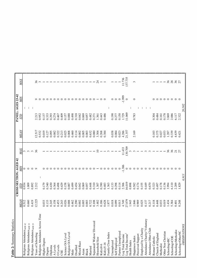
positive or negative effect on religious attendance, i.e. 01 or 01 . Full summary

statistics relating to both the cross-section data and the panel data are presented in Table 2 in

the Appendix.

IV. Results

Cross-Section Results

Exogenous Education

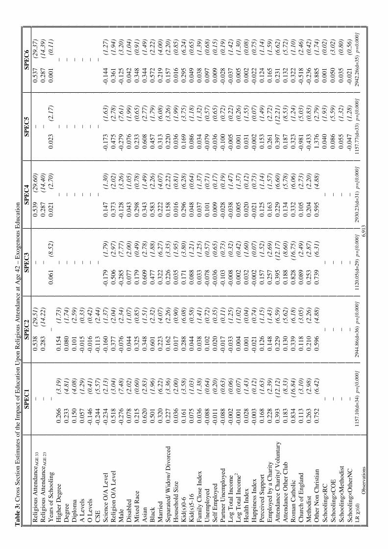
Table 3 in the Appendix presents the results derived from the cross-section analysis of the

determinants of church attendance at age 42 where education is included as an exogenous

explanatory variable. In order to explore the robustness of our cross-section findings, we

present six different specifications. Specifications 1 and 2 incorporate highest educational

qualifications whilst specifications 3 to 6 are based on years of education. Specifications 2, 4

and 6 also include past church attendance, i.e. church attendance at ages 23 and 33, in order to

ascertain whether a dynamic dimension to church attendance exists.9

It is apparent from specifications 1 and 2 that educational attainment at the upper end

of the hierarchy, i.e. degrees (undergraduate and postgraduate) and having a diploma, are

positively associated with church attendance. Lower levels of education, on the other hand,

appear to have no significant impact on church attendance, with the exception of CSE only

education, which is negatively related to attendance. It is also apparent from Table 3 that

years of education, the alternative measure of educational attainment, are positively related to

church attendance.

The sizes of the estimated coefficients on the educational attainment variables (higher

degree, degree and diploma) are somewhat reduced, however, once past religious activity is

incorporated into the analysis. It is clear that past levels of church attendance are strongly

9 For reasons of brevity, we do not present the marginal effects, although these are available from the authors on request.

18

positively related to current church attendance with the association being heightened over

time. Thus, our findings support the argument of Smith et al. (1998) that the accumulation of

religious human capital provides an incentive for future religious activity. This has not been

addressed in the literature to date due to the predominant use of cross-section data. This

argument is also supported by the significant and positive estimated coefficient on the dummy

variable indicating whether the individual has an O or A level in Religious Education. Once

again, this finding is robust across the six different specifications. The findings related to the

possession of an O or A level in a science subject, however, follow a much less distinct

pattern in terms of statistical significance but are always negatively signed. This finding

provides some support for the claim that individuals become more sceptical of faith-based

claims as they acquire education in science based subjects [see Iannaccone (1998)].

Our findings with respect to gender tie in with the existing literature in that females

are found to exhibit higher levels of church attendance than males [see, for example,

Iannaccone (1998), Sawkins et al. (1997) and Brañas Garza and Neuman (2003)]. Various

arguments have been put forward to explain the finding that women appear to be ‘more

religious’ than men. For example, it may be the case that the opportunity cost of time is lower

for women due to lower wages and/or less employment opportunities. The finding may, on

the other hand, be due to gender-based personality characteristics. Whilst the sign of the

estimated coefficient on the gender dummy variable is consistent across the specifications, the

size of the estimated coefficient is subject to a degree of variability being less pronounced

when past levels of church attendance are controlled for.

Turning to the other personal characteristics, there appears to be some differences in

the level of church attendance across ethnic groups. Being black, for example, is strongly

positively correlated with church attendance, which accords with the findings of Azzi and

Ehrenberg (1975). Marital status also appears to be an important determinant of church

19

attendance with church attendance being positively related to being married – a finding,

which once again ties in with the existing literature [see Iannaccone (1998)]. Individuals who

are separated, widowed or divorced are also more likely to attend church. Similarly, the

presence of pre-school children in the household is positively associated with church

attendance whilst having older children appears to exert an insignificant influence.

We also include a number of other variables related to individuals’ perceptions about

social networks such as whether the individual feels that he/she has someone to turn to for

support and how close he/she feels their family is. These variables, however, turned out to be

insignificantly related to church attendance. In contrast to Ellison (1993), we find that the

happiness index used to proxy life satisfaction and the health index are also insignificant. Our

findings do, however, provide some support for the hypothesis of Glaeser and Sacerdote

(2002) in that church attendance is positively related to attendance at other formal group

social activities. Moreover, these findings are highly significant and robust across the six

specifications.10

Our findings also suggest that economic status does not affect religious attendance. In

particular, being unemployed or self-employed have insignificant effects upon church

attendance, whilst total household income is also found to be insignificantly related to church

attendance. Controls for whether the individual has an unemployed partner also turn out to be

insignificant across specifications.

Finally, religious denomination is clearly an important determinant of church

attendance with Non-Christians and Roman Catholics being characterised by the largest

positive and most statistically significant estimated coefficients. In specifications 5 and 6,

10 We also investigated the relationship between educational attainment and other forms of social engagement. This essentially involved adopting the same methodology as outlined in Section III but with other measures of social attendance as the dependent variable, specifically: attendance at political party meetings; charity and voluntary group meetings; and attendance at women’s groups. In each model of social attendance, as measured by the different dependent variables (each ordered in the same way as the church attendance index), we found a positive and significant impact of education upon attendance in accordance with Glaeser and Sacerdote (2002).

20

however, when religious denomination is interacted with years of education, we find that the

Church of England denomination interaction is characterised by the most robust positive

influence.

Endogenous Education

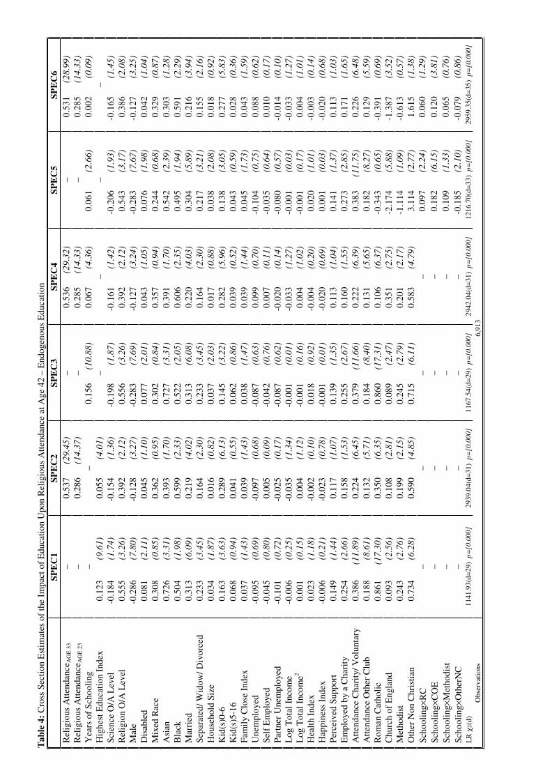
In Table 4, we repeat our cross-section analysis but replace the highest educational dummy

variables and years of education with their predicted values as derived from the educational

attainment equation outlined in Section III [see Equations 2a and 2b].11 Table 4 has the same

format as Table 3 with six specifications reported. In general, our findings are unchanged and,

hence, for reasons of brevity we will only comment on those variables, which are the focus of

our paper – namely education and past levels of religious activity. It is apparent from Table 4

that the positive association between educational attainment and church attendance remains

once educational attainment is treated as an endogenous variable. Furthermore, the sizes of

the estimated coefficients on education are much larger when education is treated as an

endogenous variable.

Thus, our findings contrast with those of Sander (2002) for the U.S. who finds no

causal effect of education on religious activities. In addition, we also find that the relationship

between current and past church attendance is robust to such changes with past levels of

religious activity being positively and strongly correlated with current church attendance. In

terms of the denomination interactions with years of schooling, i.e. specifications 5 and 6,

11 For reasons of brevity, we do not present the results pertaining to the two educational attainment equations. In general, the two equations are well-specified and our findings accord with the existing literature and a prioriexpectations. For example, the pupil-teacher ratio is found to be a significant determinant of educational attainment. Attending a grammar school is positively related to educational attainment. Family background is found to be an important determinant of education – for example parent’s years of education and whether the parents express an interest in their child’s education are both positively associated with educational attainment. Ability as proxied by test scores in maths and English at ages 7, 11 and 16 are all positively related to educational attainment. Full results are available from the authors on request.

21

again the Church of England interaction dominates and is significant, as found under the

exogenous education model.12

Panel Data Results

In Table 5 in the Appendix, we present our estimates of Equations 3, 5a and 5b for our

balanced panel of data. We omit the explanatory variables related to past religious behaviour,

as these become observations in our panel of data. In the first specification, it is apparent that

educational attainment at all levels (with the exception of CSE only education) are positively

associated with church attendance. Furthermore, the sizes of the estimated coefficients on the

educational attainment variables increase as we move up the educational attainment hierarchy.

In the next column, we endogenise the education attainment index. Our findings confirm the

positive association between church attendance and educational attainment. In the final

columns of Table 5, we explore the alternative measure of education, years of schooling.

When treated as an exogenous or endogenous variable, our findings once again support a

positive relationship between education and religion. As in the cross-section analysis, when

religious denomination is interacted with years of education, we find that the Church of

England denomination interaction is characterised by a positive influence. In addition, in

contrast to the cross-section findings, there is clear support for the claim that individuals

become more sceptical of faith-based claims as they acquire more education in science based

subjects (i.e. Biology, Chemistry or Physics), since across the panel data specifications, the

science dummy is characterised by a negative and significant estimated coefficient.

Finally, as mentioned in Section III, the magnitude of provides information

pertaining to whether individuals are likely to report consistent levels of religious activity

12 We have also conducted the analysis presented in Tables 3 and 4 for males and females separately. In general, the pattern of our results does not change. There are, however, some interesting differences between the findings for men and women. For example, the extent to which the positive association between past and current church attendance is heightened over time is much more pronounced amongst men. In addition, the impact of educational attainment on church attendance is greater for females than males – this is especially the case at higher levels of education. Full results are available from the authors on request.

22

across the three time periods or whether religious activity is subject to much change over the

individual’s life cycle. Across all of the specifications presented in Table 5, it is apparent that

is significant and, furthermore, the size of indicates that levels of church attendance are

relatively consistent over the time period.

In order to explore whether levels of church attendance vary less towards the later

stages of an individual’s life cycle, we split our panel of data into two time periods – 1981

and 1991 (i.e. ages 23 and 33) and 1991 and 2000 (i.e. ages 33 and 42). Hence, we

constructed two balanced panels of data, each with 2 6,834 (i.e. 13,668) observations. We

then repeated our analysis of Table 5 for each of the two time periods. Table 6 presents the

values of estimated for each of the twelve regressions. It is apparent that the size of is

much larger in the later time period suggesting that there is less variation in church

attendance, as individuals become older. Such an effect may be due to, for example, habit

formation over time. This supports the notion that church attendance varies less at later stages

of the life cycle.

V Conclusion

In this paper, we have contributed to the expanding area of the economics of religion, which

is one area of household behaviour that has attracted very little interest in the economics

literature. To be specific, we have explored the determinants of one measure of religious

activity – church attendance – at the individual level using British panel data derived from the

National Child Development Study. Moreover, we have focused on the relationship between

church attendance and education, which has attracted some attention in the existing literature.

We have further developed the approach of Sander (2002), who treats education as an

endogenous variable, in three main ways. Firstly, we have expanded the church attendance

equation to incorporate a more extensive array of explanatory variables. Secondly, we have

23

specified a more comprehensive educational attainment equation in order to control for

endogeneity bias. Thirdly, we have analysed individual panel data thereby enabling us to

explore religious activity from a dynamic perspective, i.e. at different points of an individual’s

life cycle – namely at ages 23, 33 and 42. In contrast to the previous literature in this area, our

data has enabled us to ascertain whether a dynamic dimension to religious activity exists.

The findings from our cross-section and panel data analysis support a positive

association between education and church attendance. In addition, our findings suggest that

current participation in religious activities is positively associated with past religious

activities. Furthermore, our results suggest that levels of religious activity tend to vary less

over time suggesting that factors such as habit formation may be important. To summarise,

our findings do suggest that a time dimension to religious activity exists. Furthermore, the

importance of previous religious activity in determining current levels of religious activity

suggests that omitting such factors from econometric analysis may lead to biased results and

erroneous inferences.

Finally, as pointed out by Sacerdote and Glaeser (2002), the positive association

between education and church attendance indicates that education plays an important role in

social involvement. Such findings may inform Governments on the reasons behind social

exclusion and may help to shape policies to alleviate social exclusion. It is apparent that

education and schooling serve to affect involvement in formal social activities such as church

attendance during adulthood. Thus, education clearly impacts upon many aspects of

household behaviour both during childhood and adulthood and, thus, may help to enhance

social inclusion.

24

References

Arulampalam, W. (1999) ‘Practitioners’ Corner: A Note on Estimated Coefficients in

Random Effects Probit Models,’ Oxford Bulletin of Economics and Statistics, 61, 597-

602.

Azzi, C. and R. Ehrenberg (1975) ‘Household Allocation of Time and Church Attendance,’

Journal of Political Economy, 83, 27-56.

Barro, R. and R. McCleary (2002) ‘Religion and Political Economy in an International Panel,’

NBER Working Paper Number: 8931.

Becker, G. S. (1981) A Treatise on the Family, Cambridge: Havard University Press.

Brañas Garza, P. and S. Neuman (2003) ‘Analysing Religiosity within an Economic

Framework: The case of Spanish Catholics,’ IZA Discussion Paper, Number 868.

Butler, J.S. and R. Moffitt (1982) ‘A Computationally Efficient Quadrature Procedure for the

One Factor Multinomial Probit Model,’ Econometrica, 50, 761-64.

Dearden, L., J. Ferri and C. Meghir (2002) ‘The Effect of School Quality on Educational

Attainment and Wages,’ The Review of Economics and Statistics, 84, 1-20.

Dustmann, C., N. Rajah and A. van Soest (2003) ‘Class Size, Education and Wages,’ The

Economic Journal, 113, F99-F120.

Ellison, C. G. (1993) ‘Religion, the Life Stress Paradigm, and the Study of Depression,’ in

Religion in Aging and Mental Health: Theoretical Foundations and Methodological

Frontiers. Jeffrey S. Levin (Editor), Thousand Oaks: Sage, 78-121.

Ermisch, J. and M. Francesconi (2001) ‘Family Matters: Impacts of Family Background on

Educational Attainment,’ Economica, 68, 137-56.

Glaeser, E. L. and B. I. Sacerdote (2002) ‘Education and Religion,’ NBER Working Paper

Number: 8080.

25

Heckman, J. and S. Cameron (1998) ‘Life Cycle Schooling and Dynamic Selection Bias:

Models and Evidence for Five Cohorts of American Males,’ Journal of Political

Economy, 106, 262-333.

Iannaccone, L. R. (1998) ‘Introduction to the Economics of Religion,’ Journal of Economic

Literature, 36, 1465-95.

Neuman, S. (1986) ‘Religious Observance within a Human Capital Framework,’ Applied

Economics, 18, 1193-1202.

Sander, W. (2002) ‘Religion and Human Capital,’ Economics Letters, 75, 303-7.

Sawkins, J. W., P. T. Seaman and H. C. S. Williams (1997) ‘Church Attendance in Great

Britain: An Ordered Logit Approach,’ Applied Economics, 29, 125-34.

Smith, I., J. W. Sawkins and P. T. Seaman (1998) ‘The Economics of Religious Participation:

A Cross-Country Study,’ Kyklos, 51, 25-43.

Stark, R., Iannaccone, L. and R. Finke (1996) ‘Religion, Science and Rationality,’ American

Economic Review, AEA Papers and Proceedings, 86, 433-7.

Tab

le 1

A:

Cro

ss T

abul

atio

ns o

f R

elig

ious

Atte

ndan

ce O

ver

Tim

e

1991

AG

E 3

3

2000

AG

E 4

2

0 1

2 3

Tot

al

0

1 2

3 T

otal

0

3,86

7

(72.

89)

1,06

1

(20.

0)

126

(2.3

8)

251

(4.7

3)

5,30

5

(77.

63)

0

3,63

7

(86.

33)

416

(9.8

7)

78

(1.8

5)

82

(1.9

5)

4,21

3

(61.

65)

1

216

(29.

71)

318

(43.

74)

76

(10.

45)

117

(16.

09)

727

(10.

64)

1

994

(64.

88)

396

(25.

85)

82

(5.3

5)

60

(3.9

2)

1,53

2

(22.

42)

1981

AG

E 2

3

255

(21.

65)

78

(30.

71)

35

(13.

78)

86

(33.

86)

254

(3.7

2)

1991

AG

E 3

3

297

(35.

14)

80

(28.

99)

56

(20.

29)

43

(15.

58)

276

(4.0

4)

3

75

(13.

69)

75

(13.

69)

39

(7.1

2)

359

(65.

51)

548

(8.0

2)

3

134

(16.

48)

139

(17.

10)

131

(16.

11)

409

(50.

31)

813

(11.

90)

T

otal

4,

213

(61.

65)

1,53

2

(22.

42)

276

(4.0

4)

813

(11.

90)

6,83

4

(100

)

T

otal

4,

862

(71.

14)

1,03

1

(15.

09)

347

(5.0

8)

594

(8.6

9)

6,83

4

(100

)

Not

e fi

gure

s in

par

enth

esis

are

per

cent

ages

.

Atte

ndan

ce f

requ

enci

es: 0

=‘n

ever

or

very

rar

ely’

; 1=

‘som

etim

es, b

ut le

ss th

an o

nce

a m

onth

’; 2

=‘o

nce

a m

onth

or

mor

e’ a

nd 3

=‘o

nce

a w

eek’

.

Tab

le 1

B:

Cro

ss T

abul

atio

ns o

f R

elig

ious

Den

omin

atio

n O

ver

Tim

e

1991

AG

E 3

3

2000

AG

E 4

2

0 1

2 3

4 T

otal

0 1

2 3

4 T

otal

0

2,39

3

(78.

98)

533

(17.

59)

69

(2.2

8)

21

(0.6

9)

14

(0.4

6)

3,03

0

(44.

34)

0

2,17

5

(56.

71)

1,28

1

(33.

40)

213

(5.5

5)

112

(2.9

2)

54

(1.4

1)

3,83

5

(56.

12)

1

822

(33.

58)

1,59

2

(65.

03)

17

(0.6

9)

16

(0.6

5)

1

(0.0

4)

2,44

8

(35.

82)

1

391

(17.

92)

1,75

7

(80.

52)

12

(0.5

5)

17

(0.7

8)

5

(0.2

3)

2,18

2

(31.

93)

1981

AG

E 2

3

216

1

(23.

20)

5

(0.7

2)

527

(75.

94)

0

(0.0

0)

1

(0.1

4)

694

(10.

16)

1991

AG

E

223

(3.7

4)

13

(1.9

5)

577

(93.

82)

0

(0.0

0)

3

(0.4

9)

615

(9.0

0)

3

81

(42.

63)

25

(13.

16)

0

(0.0

0)

84

(44.

21)

0

(0.0

0)

190

(2.7

8)

3

21

(16.

28)

11

(8.5

3)

0

(0.0

0)

97

(75.

19)

0

(0.0

0)

129

(1.8

9)

4

378

(80.

08)

27

(5.7

2)

2

(0.4

2)

8

(1.6

9)

57

(12.

08)

472

(6.9

1)

4

6

(8.2

2)

1

(1.3

7)

1

(1.3

7)

0

(0.0

0)

65

(89.

04)

73

(1.0

7)

T

otal

3,

835

(56.

12)

2,18

2

(31.

93)

615

(9.0

0)

129

(1.8

9)

73

(1.0

7)

6,83

4

(100

)

T

otal

2,

616

(38.

28)

3,06

2

(44.

81)

803

(11.

75)

226

(3.3

1)

127

(1.8

6)

6,83

4

(100

)

Not

e fi

gure

s in

par

enth

esis

are

per

cent

ages

.

Den

omin

atio

n ca

tego

ries

: 0=

No

Rel

igio

n; 1

=C

hurc

h of

Eng

land

; 2=

Rom

an C

atho

lic; 3

=M

etho

dist

and

4=

Oth

er N

on-C

hris

tian

.

Tab

le 2

: Su

mm

ary

Stat

istic

s

CR

OSS

SE

CT

ION

: A

GE

D 4

2 P

AN

EL

: A

GE

S 23

-42

ME

AN

ST

D

MIN

M

AX

M

EA

N

STD

M

IN

MA

XR

elig

ious

Att

enda

nce A

GE

42

0.51

2 0.

934

0 3

–R

elig

ious

Att

enda

nce A

GE

33

0.66

0 1.

009

0 3

–R

elig

ious

Att

enda

nce A

GE

23

0.41

9 0.

892

0 3

–Y

ears

of

Sch

ooli

ng

12.2

25

2.21

2 9

36

12.5

17

2.21

3 9

36

Rel

igio

us A

tten

danc

e A

cros

s T

ime

–0.

532

0.95

2 0

3 H

ighe

r D

egre

e 0.

033

0.17

9 0

1 0.

019

0.13

7 0

1 D

egre

e 0.

133

0.34

0 0

1 0.

127

0.33

3 0

1 D

iplo

ma

0.24

5 0.

430

0 1

0.09

5 0.

293

0 1

A L

evel

s 0.

158

0.36

4 0

1 0.

082

0.27

4 0

1 O

Lev

els

0.45

3 0.

498

0 1

0.32

2 0.

467

0 1

CS

E

0.24

3 0.

429

0 1

0.21

3 0.

409

0 1

Sci

ence

O/A

Lev

el

0.02

6 0.

158

0 1

0.02

5 0.

157

0 1

Rel

igio

n O

/A L

evel

0.

008

0.08

7 0

1 0.

008

0.08

8 0

1 M

ale

0.46

2 0.

499

0 1

0.46

0 0.

498

0 1

Dis

able

d 0.

290

0.45

4 0

1 0.

114

0.31

8 0

1 M

ixed

Rac

e 0.

002

0.04

2 0

1 0.

002

0.04

2 0

1 A

sian

0.

005

0.06

9 0

1 0.

005

0.06

9 0

1 B

lack

0.

003

0.05

7 0

1 0.

003

0.05

7 0

1 M

arri

ed

0.72

2 0.

448

0 1

0.63

2 0.

482

0 1

Sep

arat

ed/ W

idow

/ Div

orce

d 0.

108

0.31

0 0

1 0.

080

0.27

1 0

1 H

ouse

hold

Siz

e 3.

482

1.30

7 1

10

3.30

4 1.

361

1 24

K

id(s

)0-6

0.

186

0.39

0 0

1 0.

268

0.44

3 0

1 K

id(s

)5-1

6 0.

628

0.48

3 0

1 0.

384

0.48

6 0

1 F

amil

y C

lose

Ind

ex

1.87

7 1.

363

0 3

–U

nem

ploy

ed

0.01

8 0.

133

0 1

0.03

8 0.

190

0 1

Sel

f E

mpl

oyed

0.

099

0.29

8 0

1 0.

084

0.27

7 0

1 P

artn

er U

nem

ploy

ed

0.01

3 0.

114

0 1

0.02

3 0.

150

0 1

Log

Tot

al I

ncom

e 4.

749

2.30

6 -1

.386

11

.433

4.

286

1.72

9 -1

.999

11

.736

L

og T

otal

Inc

ome2

27.8

79

16.0

19

0 13

0.70

9 21

.357

11

.069

0

137.

735

Hea

lth

Inde

x 1.

945

0.89

8 0

3 –

Hap

pine

ss I

ndex

1.

846

0.58

2 0

3 2.

169

0.78

3 0

3 P

erce

ived

Sup

port

0.

969

0.17

4 0

1 –

Em

ploy

ed b

y a

Cha

rity

0.

025

0.15

5 0

1 –

Att

enda

nce

Cha

rity

/ Vol

unta

ry

0.13

7 0.

449

0 3

–A

tten

danc

e O

ther

Clu

b 0.

217

0.67

0 0

3 –

Rom

an C

atho

lic

0.11

8 0.

323

0 1

0.10

3 0.

304

0 1

Chu

rch

of E

ngla

nd

0.44

8 0.

497

0 1

0.37

5 0.

484

0 1

Met

hodi

st

0.03

3 0.

178

0 1

0.02

7 0.

161

0 1

Oth

er N

on C

hris

tian

0.

019

0.13

6 0

1 0.

033

0.17

8 0

1 S

choo

ling

RC

1.43

4 3.

994

0 36

1.

287

3.86

9 0

36

Sch

ooli

ngC

OE

5.38

4 6.

110

0 36

0.

339

2.08

6 0

28

Sch

ooli

ngM

etho

dist

0.

401

2.20

9 0

21

4.63

9 6.

117

0 36

S

choo

ling

Oth

erN

C

0.24

8 1.

829

0 27

0.

421

2.32

2 0

27

OB

SER

VA

TIO

NS

6,91

3 20

,502

Tab

le 3

: C

ross

Sec

tion

Est

imat

es o

f th

e Im

pact

of

Edu

cati

on U

pon

Rel

igio

us A

tten

danc

e at

Age

42

– E

xoge

nous

Edu

cati

on

SPE

C1

SPE

C2

SPE

C3

SPE

C4

SPE

C5

SPE

C6

Rel

igio

us A

ttend

ance

AG

E 3

3 –

0.53

8(2

9.51

)

– 0.

539

(29.

60)

–

0.53

7 (2

9.37

) R

elig

ious

Atte

ndan

ceA

GE

23

–0.

283

(14.

22)

–

0.28

7 (1

4.40

)

– 0.

287

(14.

39)

Yea

rs o

f Sc

hool

ing

– –

0.06

1 (8

.52)

0.02

1 (2

.70)

0.02

3 (2

.17)

0.00

1 (0

.11)

H

ighe

r D

egre

e 0.

266

(3.1

9)

0.

154

(1.7

3)

–

– –

– D

egre

e 0.

233

(4.8

1)

0.

080

(1.7

4)

–

– –

– D

iplo

ma

0.15

0 (4

.08)

0.10

1 (2

.59)

– –

– –

A L

evel

s 0.

057

(1.2

9)

-0

.015

(0

.33)

– –

– –

O L

evel

s -0

.146

(0

.41)

-0.0

16

(0.4

2)

–

– –

– C

SE

-0.2

44

(5.5

7)

-0

.113

(2

.44)

– –

– –

Scie

nce

O/A

Lev

el

-0.2

34

(2.1

3)

-0

.160

(1

.37)

-0.1

79

(1.7

9)

0.

147

(1.3

0)

-0

.173

(1

.63)

-0.1

44

(1.2

7)

Rel

igio

n O

/A L

evel

0.

518

(3.0

4)

0.

377

(2.0

4)

0.

506

(2.9

7)

0.

373

(2.0

2)

0.

475

(2.7

8)

0.

361

(1.9

4)

Mal

e -0

.276

(7

.48)

-0.0

76

(2.3

4)

-0

.285

(7

.77)

-0.1

28

(3.2

6)

-0

.279

(7

.61)

-0.1

25

(3.2

0)

Dis

able

d 0.

078

(2.0

2)

0.

044

(1.0

7)

0.

077

(2.0

0)

0.

043

(1.0

5)

0.

076

(1.9

9)

0.

042

(1.0

4)

Mix

ed R

ace

0.21

5 (0

.60)

0.32

5 (0

.85)

0.17

9 (0

.49)

0.29

8 (0

.78)

0.23

3 (0

.65)

0.34

8 (0

.91)

A

sian

0.

620

(2.8

3)

0.

348

(1.5

1)

0.

609

(2.7

8)

0.

343

(1.4

9)

0.

608

(2.7

7)

0.

344

(1.4

9)

Bla

ck

0.50

1 (1

.96)

0.60

1 (2

.32)

0.47

7 (1

.88)

0.58

3 (2

.26)

0.45

7 (1

.79)

0.57

2 (2

.22)

M

arri

ed

0.32

0 (6

.22)

0.22

3 (4

.07)

0.32

2 (6

.27)

0.22

2 (4

.07)

0.31

3 (6

.08)

0.21

9 (4

.00)

Se

para

ted/

Wid

ow/ D

ivor

ced

0.22

7 (3

.36)

0.16

2 (2

.26)

0.22

6 (3

.35)

0.15

8 (2

.22)

0.22

0 (3

.26)

0.15

7 (2

.20)

H

ouse

hold

Siz

e 0.

036

(2.0

0)

0.

017

(0.9

0)

0.

035

(1.9

5)

0.

016

(0.8

1)

0.

036

(1.9

9)

0.

016

(0.8

5)

Kid

(s)0

-6

0.16

1 (3

.58)

0.28

8 (6

.08)

0.17

1 (3

.80)

0.29

6 (6

.28)

0.16

9 (3

.75)

0.29

5 (6

.24)

K

id(s

)5-1

6 0.

075

(1.0

3)

0.

044

(0.5

8)

0.

088

(1.2

1)

0.

048

(0.6

4)

0.

086

(1.1

8)

0.

049

(0.6

5)

Fam

ily

Clo

se I

ndex

0.

036

(1.3

8)

0.

038

(1.4

1)

0.

033

(1.2

5)

0.

037

(1.3

7)

0.

034

(1.3

2)

0.

038

(1.3

9)

Une

mpl

oyed

-0

.088

(0

.64)

0.10

2 (0

.72)

-0.0

78

(0.5

7)

0.

101

(0.7

1)

-0

.079

(0

.57)

0.09

7 (0

.68)

Se

lf E

mpl

oyed

-0

.011

(0

.20)

0.02

0 (0

.35)

-0.0

36

(0.6

5)

0.

009

(0.1

7)

-0

.036

(0

.65)

0.00

9 (0

.15)

P

artn

er U

nem

ploy

ed

-0.0

88

(0.6

3)

-0

.017

(0

.11)

-0.1

03

(0.7

3)

-0

.028

(0

.19)

-0.1

00

(0.7

2)

-0

.028

(0

.19)

L

og T

otal

Inc

ome

-0.0

02

(0.0

6)

-0

.033

(1

.25)

-0.0

08

(0.3

2)

-0

.038

(1

.47)

-0.0

05

(0.2

2)

-0

.037

(1

.42)

L

og T

otal

Inc

ome2

-0.0

01

(0.0

7)

0.

004

(1.0

2)

0.

002

(0.4

2)

0.

005

(1.3

7)

0.

001

(0.2

6)

0.

005

(1.3

0)

Hea

lth

Inde

x 0.

028

(1.4

3)

0.

001

(0.0

4)

0.

032

(1.6

0)

0.

020

(0.1

2)

0.

031

(1.5

5)

0.

002

(0.0

8)

Hap

pine

ss I

ndex

-0

.003

(0

.12)

-0.0

21

(0.7

4)

-0

.002

(0

.07)

-0.0

21

(0.7

3)

-0

.002

(0

.07)

-0.0

22

(0.7

5)

Per

ceiv

ed S

uppo

rt

0.16

8 (1

.63)

0.12

6 (1

.15)

0.15

7 (1

.52)

0.12

5 (1

.14)

0.15

3 (1

.49)

0.12

4 (1

.14)

E

mpl

oyed

by

a C

hari

ty

0.22

8 (2

.39)

0.14

8 (1

.43)

0.25

7 (2

.69)

0.16

3 (1

.57)

0.26

1 (2

.72)

0.16

5 (1

.59)

A

tten

danc

e C

hari

ty/ V

olun

tary

0.

393

(12.

12)

0.

229

(6.5

9)

0.

395

(12.

17)

0.

229

(6.6

0)

0.

397

(12.

21)

0.

231

(6.6

2)

Att

enda

nce

Oth

er C

lub

0.18

3 (8

.33)

0.13

0(5

.62)

0.18

8 (8

.60)

0.13

4 (5

.78)

0.18

7 (8

.53)

0.13

2 (5

.72)

R

oman

Cat

holic

0.

834

(16.

84)

0.

339

(6.1

8)

0.

828

(16.

75)

0.

332

(6.0

6)

0.

323

(1.2

4)

0.

322

(1.1

0)

Chu

rch

of E

ngla

nd

0.11

3 (3

.10)

0.11

8(3

.05)

0.08

9 (2

.49)

0.10

5 (2

.73)

-0.9

81

(5.0

3)

-0

.518

(2

.46)

M

etho

dist

0.

263

(2.9

8)

0.

210

(2.2

6)

0.

253

(2.8

7)

0.

204

(2.2

0)

-0

.433

(0

.83)

-0.2

36

(0.4

2)

Oth

er N

on C

hris

tian

0.75

2 (6

.42)

0.59

6(4

.88)

0.73

9 (6

.31)

0.59

5 (4

.88)

1.37

6 (2

.79)

0.88

5 (1

.74)

Sc

hool

ing

RC

–

––

– 0.

040

(1.9

3)

0.

001

(0.0

2)

Scho

olin

gC

OE

–

– –

– 0.

086

(5.5

9)

0.

050

(3.0

2)

Scho

olin

gM

etho

dist

–

– –

– 0.

055

(1.3

2)

0.

035

(0.8

0)

Scho

olin

gO

ther

NC

–

– –

– -0

.047

(1

.28)

-0.0

21

(0.5

6)

LR

2(

d)

1157

.10(

d=34

) p

=[0

.000

] 29

44.8

6(d=

36)

p=

[0.0

00]

1120

.05(

d=29

) p

=[0

.000

] 29

30.2

3(d=

31)

p=

[0.0

00]

1157

.77(

d=33

) p

=[0

.000

] 29

42.2

6(d=

35)

p=

0.00

0]

Obs

erva

tion

s 6,

913

Tab

le 4

: C

ross

Sec

tion

Est

imat

es o

f th

e Im

pact

of

Edu

cati

on U

pon

Rel

igio

us A

tten

danc

e at

Age

42

– E

ndog

enou

s E

duca

tion

SPE

C1

SPE

C2

SPE

C3

SPE

C4

SPE

C5

SPE

C6

Rel

igio

us A

ttend

ance

AG

E 3

3 –

0.53

7(2

9.45

)

– 0.

536

(29.

32)

–

0.53

1 (2

8.99

) R

elig

ious

Atte

ndan

ceA

GE

23

–0.

286

(14.

37)

–

0.28

5 (1

4.33

)

– 0.

285

(14.

33)

Yea

rs o

f Sc

hool

ing

– –

0.15

6 (1

0.88

)

0.06

7 (4

.36)

0.06

1 (2

.66)

0.00

2 (0

.09)

H

ighe

st E

duca

tion

Ind

ex

0.12

3 (9

.61)

0.05

5 (4

.01)

– –

– –

Scie

nce

O/A

Lev

el

-0.1

84

(1.7

4)

-0

.154

(1

.36)

-0.1

98

(1.8

7)

-0

.161

(1

.42)

-0.2

06

(1.9

3)

-0

.165

(1

.45)

R

elig

ion

O/A

Lev

el

0.55

5 (3

.26)

0.39

2 (2

.12)

0.55

6 (3

.26)

0.39

2 (2

.12)

0.54

3 (3

.17)

0.38

6 (2

.08)

M

ale

-0.2

86

(7.8

0)

-0

.128

(3

.27)

-0.2

83

(7.6

9)

-0

.127

(3

.24)

-0.2

83

(7.6

7)

-0

.127

(3

.25)

D

isab

led

0.08

1 (2

.11)

0.04

5 (1

.10)

0.07

7 (2

.01)

0.04

3 (1

.05)

0.07

6 (1

.98)

0.04

2 (1

.04)

M

ixed

Rac

e 0.

308

(0.8

5)

0.

362

(0.9

5)

0.

302

(0.8

4)

0.

357

(0.9

4)

0.

244

(0.6

8)

0.

329

(0.8

7)

Asi

an

0.72

6 (3

.31)

0.39

3 (1

.70)

0.72

7 (3

.31)

0.39

1 (1

.70)

0.54

2 (2

.39)

0.30

3 (1

.28)

B

lack

0.

504

(1.9

8)

0.

599

(2.3

3)

0.

522

(2.0

5)

0.

606

(2.3

5)

0.

495

(1.9

4)

0.

591

(2.2

9)

Mar

ried

0.

313

(6.0

9)

0.

219

(4.0

2)

0.

313

(6.0

8)

0.

220

(4.0

3)

0.

304

(5.8

9)

0.

216

(3.9

4)

Sepa

rate

d/ W

idow

/ Div

orce

d 0.

233

(3.4

5)

0.

164

(2.3

0)

0.

233

(3.4

5)

0.

164

(2.3

0)

0.

217

(3.2

1)

0.

155

(2.1

6)

Hou

seho

ld S

ize

0.03

4 (1

.87)

0.01

6 (0

.82)

0.03

7 (2

.03)

0.01

7 (0

.88)

0.03

8 (2

.08)

0.01

8 (0

.92)

K

id(s

)0-6

0.

163

(3.6

3)

0.

289

(6.1

3)

0.

145

(3.2

2)

0.

282

(5.9

6)

0.

138

(3.0

5)

0.

277

(5.8

3)

Kid

(s)5

-16

0.06

8 (0

.94)

0.04

1 (0

.55)

0.06

2 (0

.86)

0.03

9 (0

.52)

0.04

3 (0

.59)

0.02

8 (0

.36)

Fa

mil

y C

lose

Ind

ex

0.03

7 (1

.43)

0.03

9 (1

.43)

0.03

8 (1

.47)

0.03

9 (1

.44)

0.04

5 (1

.73)

0.04

3 (1

.59)

U

nem

ploy

ed

-0.0

95

(0.6

9)

-0

.097

(0

.68)

-0.0

87

(0.6

3)

0.

099

(0.7

0)

-0

.104

(0

.75)

0.08

8 (0

.62)

Se

lf E

mpl

oyed

-0

.045

(0

.80)

0.00

5 (0

.09)

-0.0

42

(0.7

6)

0.

007

(0.1

1)

-0

.035

(0

.64)

0.01

0 (0

.17)

P

artn

er U

nem

ploy

ed

-0.1

01

(0.7

2)

-0

.025

(0

.17)

-0.0

87

(0.6

2)

-0

.020

(0

.14)

-0.0

80

(0.5

7)

-0

.014

(0

.10)

L

og T

otal

Inc

ome

-0.0

06

(0.2

5)

-0

.035

(1

.34)

-0.0

01

(0.0

1)

-0

.033

(1

.27)

-0.0

01

(0.0

3)

-0

.033

(1

.27)

L

og T

otal

Inc

ome2

0.00

1 (0

.15)

0.00

4 (1

.12)

-0.0

01

(0.1

6)

0.

004

(1.0

2)

-0

.001

(0

.17)

0.00

4 (1

.01)

H

ealt

h In

dex

0.02

3 (1

.18)

-0.0

02

(0.1

0)

0.

018

(0.9

2)

-0

.004

(0

.20)

0.02

0 (1

.01)

-0.0

03

(0.1

4)

Hap

pine

ss I

ndex

-0

.006

(0

.21)

-0.0

23

(0.7

8)

-0

.001

(0

.01)

-0.0

20

(0.6

9)

0.

001

(0.0

3)

-0

.020

(0

.68)

P

erce

ived

Sup

port

0.

149

(1.4

4)

0.

117

(1.0

7)

0.

139

(1.3

5)

0.

113

(1.0

4)

0.

141

(1.3

7)

0.

113

(1.0

3)

Em

ploy

ed b

y a

Cha

rity

0.

254

(2.6

6)

0.

158

(1.5

3)

0.

255

(2.6

7)

0.

160

(1.5

5)

0.

273

(2.8

5)

0.

171

(1.6

5)

Att

enda

nce

Cha

rity

/ Vol

unta

ry

0.38

6 (1

1.89

)

0.22

4 (6

.45)

0.37

9 (1

1.66

)

0.22

2 (6

.39)

0.38

3 (1

1.75

)

0.22

6 (6

.48)

A

tten

danc

e O

ther

Clu

b 0.

188

(8.6

1)

0.

132

(5.7

1)

0.

184

(8.4

0)

0.

131

(5.6

5)

0.

182

(8.2

7)

0.

129

(5.5

9)

Rom

an C

atho

lic

0.86

1 (1

7.30

)

0.35

0(6

.35)

0.86

0 (1

7.31

)

0.10

6 (6

.37)

-0.3

43

(0.6

5)

-0

.391

(0

.69)

C

hurc

h of

Eng

land

0.

093

(2.5

6)

0.

108

(2.8

1)

0.

089

(2.4

7)

0.

351

(2.7

5)

-2

.174

(5

.88)

-1.3

87

(3.5

2)

Met

hodi

st

0.24

3 (2

.76)

0.19

9(2

.15)

0.24

5 (2

.79)

0.20

1 (2

.17)

-1.1

14

(1.0

9)

-0

.613

(0

.57)

O

ther

Non

Chr

istia

n 0.

734

(6.2

8)

0.

590

(4.8

5)

0.

715

(6.1

1)

0.

583

(4.7

9)

3.

114

(2.7

7)

1.

615

(1.3

8)

Scho

olin

gR

C

– –

– –

0.09

7 (2

.24)

0.06

0 (1

.29)

Sc

hool

ing

CO

E

– –

– –

0.18

2 (6

.15)

0.12

0(3

.81)

Sc

hool

ing

Met

hodi

st

– –

– –

0.10

9 (1

.33)

0.06

5 (0

.76)

Sc

hool

ing

Oth

erN

C

– –

– –

-0.1

85

(2.1

0)

-0

.079

(0

.86)

L

R

2(d)

11

41.9

3(d=

29)

p=

[0.0

00]

2939

.04(

d=31

) p

=[0

.000

] 11

67.5

4(d=

29)

p=

[0.0

00]

2942

.04(

d=31

) p

=[0

.000

] 12

16.7

0(d=

33)

p=

[0.0

00]

2959

.35(

d=35

) p

=[0

.000

] O

bser

vati

ons

6,91

3

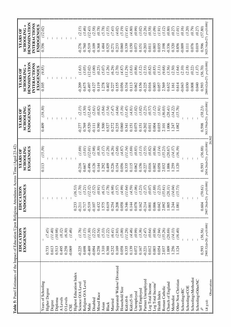
Tab

le 5

: P

anel

Est

imat

es o

f th

e Im

pact

of

Edu

cati

on U

pon

Rel

igio

us A

tten

danc

e A

cros

s T

ime

(Age

d 23

-42)

ED

UC

AT

ION

E

XO

GE

NO

US

ED

UC

AT

ION

E

ND

OG

EN

OU

S Y

EA

RS

OF

SC

HO

OL

ING

E

XO

GE

NO

US

YE

AR

S O

F

SCH

OO

LIN

G

EN

DO

GE

NO

US

YE

AR

S O

F

SCH

OO

LIN

G +

D

EN

OM

INA

TIO

N

INT

ER

AC

TIO

NS

EX

OG

EN

OU

S

YE

AR

S O

F

SCH

OO

LIN

G +

D

EN

OM

INA

TIO

N

INT

ER

AC

TIO

NS

EN

DO

GE

NO

US

Yea

rs o

f Sc

hool

ing

– –

0.11

3 (1

5.39

)

0.40

9 (1

9.30

)

0.10

5 (9

.85)

0.35

6 (1

2.02

) H

ighe

r D

egre

e 0.

733

(7.4

5)

–

––

– –

Deg

ree

0.61

3 (1

1.40

)

– –

––

–D

iplo

ma

0.51

3 (1

0.98

)

– –

––

–A

Lev

els

0.49

5 (8

.32)

– –

––

–O

Lev

els

0.25

8 (6

.30)

– –

––

–C

SE

-0.0

69

(1.4

6)

–

––

––

Hig

hest

Edu

cati

on I

ndex

–

0.23

3 (1

6.53

)

––

––

Scie

nce

O/A

Lev

el

-0.2

25

(1.7

6)

-0

.211

(1

.70)

-0.2

16

(1.6

9)

-0

.277

(2

.15)

-0.2

09

(1.6

3)

-0

.276

(2

.15)

R

elig

ion

O/A

Lev

el

0.69

8 (3

.15)

0.71

7 (3

.21)

0.66

7 (3

.01)

0.76

9 (3

.50)

0.67

5 (3

.05)

0.76

0 (3

.46)

M

ale

-0.4

69

(11.

30)

-0

.519

(1

2.32

)

-0.4

96

(12.

01)

-0

.520

(1

2.43

)

-0.4

97

(12.

02)

-0

.519

(1

2.43

) D

isab

led

-0.0

94

(2.2

2)

-0

.107

(2

.52)

-0.1

26

(2.9

8)

-0

.111

(2

.61)

-0.1

27

(3.0

0)

-0

.109

(2

.58)

M

ixed

Rac

e 0.

258

(0.5

4)

0.

432

(0.9

1)

0.

144

(0.3

0)

0.

390

(0.8

2)

0.

119

(0.2

5)

0.

368

(0.7

8)

Asi

an

1.31

0 (5

.33)

1.57

5 (6

.15)

1.29

2 (5

.17)

1.50

0 (5

.84)

1.27

8 (5

.07)

1.48

4 (5

.78)

B

lack

0.

388

(1.2

2)

0.

619

(1.7

8)

0.

409

(1.2

8)

0.

527

(1.5

4)

0.

402

(1.2

6)

0.

525

(1.5

5)

Mar

ried

0.

232

(6.4

1)

0.

254

(6.9

8)

0.

226

(6.2

6)

0.

272

(7.4

7)

0.

227

(6.2

9)

0.

271

(7.4

3)

Sepa

rate

d/ W

idow

/ Div

orce

d 0.

169

(2.9

3)

0.

208

(3.5

7)

0.

154

(2.6

8)

0.

235

(4.0

4)

0.

155

(2.7

0)

0.

233

(4.0

2)

Hou

seho

ld S

ize

0.05

8 (5

.00)

0.05

8 (4

.99)

0.05

6 (4

.87)

0.06

0 (5

.16)

0.05

6 (4

.87)

0.06

0 (5

.19)

K

id(s

)0-6

0.

335

(11.

28)

0.

346

(11.

64)

0.

335

(11.

34)

0.

341

(11.

45)

0.

334

(11.

29)

0.

339

(11.

41)

Kid

(s)5

-16

0.13

9 (4

.46)

0.14

4 (4

.59)

0.11

5 (3

.69)

0.15

1 (4

.81)

0.11

3 (3

.63)

0.15

0 (4

.80)

U

nem

ploy

ed

0.07

2 (0

.99)

0.07

8 (1

.06)

0.06

2 (0

.85)

0.07

5 (1

.02)

0.06

2 (0

.86)

0.07

3 (0

.99)

Se

lf E

mpl

oyed

0.

167

(3.3

6)

0.

162

(3.2

3)

0.

156

(3.1

3)

0.

151

(3.0

2)

0.

156

(3.1

2)

0.

151

(3.0

2)

Par

tner

Une

mpl

oyed

-0

.221

(2

.47)

-0.2

14

(2.3

7)

-0

.227

(2

.55)

-0.2

02

(2.2

5)

-0

.225

(2

.53)

-0.2

03

(2.2

6)

Log

Tot

al I

ncom

e 0.

012

(0.6

4)

0.

001

(0.0

7)

0.

016

(0.8

2)

0.

011

(0.5

7)

0.

016

(0.8

2)

0.

011

(0.5

8)

Log

Tot

al I

ncom

e2 0.

003

(0.9

8)

0.

006

(1.8

8)

0.

002

(0.8

6)

0.

004

(1.1

2)

0.

003

(0.8

5)

0.

003

(1.0

9)

Hea

lth

Inde

x 0.

054

(2.9

4)

0.

042

(2.2

3)

0.

058

(3.1

4)

0.

035

(1.9

1)

0.

057

(3.1

1)

0.

035

(1.9

1)

Rom

an C

atho

lic

2.03

7 (3

5.26

)

2.09

2(3

5.61

)

2.03

2 (3

5.23

)

2.10

1 (3

6.03

)

2.56

9 (9

.68)

2.19

8 (3

.12)

C

hurc

h of

Eng

land

1.

009

(28.

69)

1.

005

(28.

31)

1.

006

(28.

67)

1.

006

(28.

41)

0.

632

(3.5

6)

-0

.336

(0

.80)

M

etho

dist

1.

256

(14.

33)

1.

244

(14.

04)

1.

259

(14.

37)

1.

247

(14.

22)

1.

161

(2.5

0)

0.

320

(0.2

7)

Oth

er N

on C

hris

tian

1.12

4 (1

6.40

)

1.08

1(1

5.73

)

1.12

0 (1

6.39

)

1.08

2 (1

5.76

)

0.61

4 (1

.64)

0.85

6 (1

.01)

Sc

hool

ing

RC

–

––

–-0

.043

(2

.10)

-0.0

09

(0.1

6)

Scho

olin

gC

OE

–

––

–0.

030

(2.1

8)

0.

111

(3.2

0)

Scho

olin

gM

etho

dist

–

––

–0.

008

(0.2

2)

0.

076

(0.7

9)

Scho

olin

gO

ther

NC

–

––

–0.

040

(1.3

7)

0.

019

(0.2

7)

0.59

3(5

6.56

)

0.60

4 (5

9.61

)

0.59

3(5

6.88

)

0.59

8 (5

8.23

)

0.59

3 (5

6.70

)

0.59

6 (5

7.80

) L

R

2(d)

29

05.5

2(d=

28)

p=

[0.0

00]

2907

.26(

d=23

) p

=[0

.000

] 28

54.2

6(d=

23)

p=

[0.0

00]

3013

.59(

d=23

) p

=[0

.000

] 28

69.6

2(d=

27)

p=

[0.0

00]

3025

.34(

d=27

) p

=[0

.000

] O

bser

vati

ons

20,5

02

Tab

le 6

: P

anel

Sam

ple

Split

Acr

oss

Tim

e ED

UC

AT

ION

E

XO

GE

NO

US

ED

UC

AT

ION

E

ND

OG

EN

OU

S Y

EA

RS

OF

SC

HO

OL

ING

E

XO

GE

NO

US

YE

AR

S O

F

SCH

OO

LIN

G

EN

DO

GE

NO

US

YE

AR

S O

F

SCH

OO

LIN

G +

D

EN

OM

INA

TIO

N

INT

ER

AC

TIO

NS

EX

OG

EN

OU

S

YE

AR

S O

F

SCH

OO

LIN

G +

D

EN

OM

INA

TIO

N

INT

ER

AC

TIO

NS

EN

DO

GE

NO

US

1981

and

199

1 (a

ged

23 &

33)

0.

564

(36.

54)

0.

572

(37.

23)

0.

555

(35.

57)

0.

571

(37.

04)

0.

556

(35.

67)

0.

570

(36.

92)

Obs

erva

tion

s 13

,668

1991

and

200

0 (a

ged

33 &

42)

0.64

4 (5

2.82

)

0.65

1 (5

4.99

)

0.64

5(5

2.29

)

0.64

8 (5

4.07

)

0.64

2 (5

2.57

)

0.64

4 (5

3.22

)

Obs

erva

tion

s 13

,668