evidence-based treatment of alcohol, drug, and mental health disorders

Summary The Washington State Institute for Public Policy was directed by the 2005 Washington Legislature to estimate whether “evidence-based” treatment for people with alcohol, drug, and mental health disorders offers economic advantages. Do benefits outweigh costs? And, if so, what is the magnitude of the potential fiscal savings to government, as well as the total net benefits to all of Washington? Methods To answer these questions, we systematically reviewed the “what works” literature regarding treatments for people with alcohol, drug, and mental health disorders. We then estimated the monetary value of the benefits, including factors such as improved performance in the job market, reduced health care and other costs, and reduced crime-related costs. Findings 1. Evidence-based treatment works. We found

that the average evidence-based treatment can achieve roughly a 15 to 22 percent reduction in the incidence or severity of these disorders—at least in the short term.

2. The economics look attractive. We found that evidenced-based treatment of these disorders can achieve about $3.77 in benefits per dollar of treatment cost. This is equivalent to a 56 percent rate of return on investment. From a narrower taxpayer’s-only perspective, the ratio is roughly $2.05 in benefits per dollar of cost.

3. The potential is significant. We estimate that a reasonably aggressive implementation policy could generate $1.5 billion in net benefits for people in Washington ($416 million are net taxpayer benefits). The risk of losing money with an evidence-based treatment policy is small.

During the mid-1990s, the Washington State legislature began to enact statutes to promote an “evidence-based” approach to several public policies. While the term evidence-based has not always been precisely defined in legislation, it has generally been constructed to describe a program or policy supported by a rigorous outcome evaluation clearly demonstrating effectiveness. Additionally, to determine if taxpayers receive an adequate return on investment, the legislature has also started to require benefit-cost analyses of certain state-funded programs and practices. Washington’s initial experiments with evidence-based and cost-beneficial public policies began in the state’s juvenile justice system. The legislature funded several nationally known and rigorously researched programs designed to reduce the reoffending rates of juveniles. At the same time, the legislature eliminated the funding of a juvenile justice program when a careful evaluation revealed that it was failing to reduce juvenile crime. Thus, the term evidence-based does not mean simply adding new programs, it also means eliminating programs when research indicates they do not work. Following this successful venture into evidence-based public policy, Washington began to introduce the approach in other fields including adult corrections, child welfare, and K–12 education. Extending the Evidence-Based Concept to the Treatment of Alcohol, Drug, and Mental Health Disorders. The 2005 Legislature directed the Washington State Institute for Public Policy (Institute) to examine the potential benefits Washington could obtain if it adopted an evidence-based approach for alcohol, drug, and mental illness treatment. This report describes our “bottom-line” findings as well as our research approach.

_____________________________________________ Suggested citation for this report:

Steve Aos, Jim Mayfield, Marna Miller, and Wei Yen. (2006). Evidence-based treatment of alcohol, drug, and mental health disorders: Potential benefits, costs, and fiscal impacts for Washington State. Olympia: Washington State Institute for Public Policy.

Washington State Institute for Public Policy

110 Fifth Avenue Southeast, Suite 214 • PO Box 40999 • Olympia, WA 98504-0999 • (360) 586-2677 • www.wsipp.wa.gov

June 2006

EVIDENCE-BASED TREATMENT OF ALCOHOL, DRUG, AND MENTAL HEALTH DISORDERS: POTENTIAL BENEFITS, COSTS, AND FISCAL IMPACTS FOR WASHINGTON STATE

2

Legislative Study Language Engrossed Second Substitute Senate Bill 5763, Chapter 504, Laws of 2005, Sec. 605.

“The Washington state institute for public policy shall study the net short-run and long-run fiscal savings to state and local governments of implementing evidence-based treatment of chemical dependency disorders, mental disorders, and co-occurring mental and substance abuse disorders. The institute shall use the results from its 2004 report entitled "Benefits and Costs of Prevention and Early Intervention Programs for Youth" and its work on effective adult corrections programs to project total fiscal impacts under alternative implementation scenarios. In addition to fiscal outcomes, the institute shall estimate the long-run effects that an evidence-based strategy could have on statewide education, crime, child abuse and neglect, substance abuse, and economic outcomes. The institute shall provide an interim report to the appropriate committees of the legislature by January 1, 2006, and a final report by June 30, 2006.”

The Institute received an appropriation of $80,000 to conduct the study.

Background: The Omnibus Treatment of Mental and Substance Abuse Disorders Act of 2005 This research assignment originated in a much larger bill enacted during the 2005 legislative session: the Omnibus Treatment of Mental and Substance Abuse Disorders Act. A major goal of the Act is to reform how publicly-funded mental health and chemical dependency programs are provided in Washington. In passing the omnibus Act, the 2005 Legislature found that:

“Persons with mental disorders, chemical dependency disorders, or co-occurring mental and substance abuse disorders are disproportionately more likely to be confined in a correctional institution, become homeless, become involved with child protective services or involved in a dependency proceeding, or lose those state and federal benefits to which they may be entitled as a result of their disorders.” 1

Further, the Legislature found that:

“Prior state policy of addressing mental health and chemical dependency in isolation from each other has not been cost-effective and has often resulted in longer-term, more costly treatment that may be less effective over time.” 2

Among the several actions adopted in the 2005 Act to address these general concerns, the Legislature indicated its intention to:

“Improve treatment outcomes by shifting treatment, where possible, to evidence-based, research-based, and consensus-based treatment practices and by removing barriers to the use of those practices.” 3

The Basic Questions for the Study Within the context of the Act’s overall goals, the language directing the Institute’s study is shown in the sidebar on this page.

1 E2SSB 5763, Chapter 504, Laws of 2005, Section 101. 2 Ibid. 3 Ibid., Section 101(3).

In brief, the Legislature directed the Institute to answer the following “bottom-line” questions:

Does evidence-based treatment for people with alcohol, drug, or mental health disorders make economic sense?

Do benefits outweigh costs?

And, if so, what is the potential magnitude of the fiscal savings to government, and what are the total net benefits to all of Washington?

In addition to directing the Institute to answer these questions, the omnibus Act also required the Institute to evaluate the effectiveness of the Act’s pilot programs, which are designed to test several new implementation approaches (see the sidebar on page 6 for a brief description of the pilot program study).

3

Research Methods To answer the Legislature’s questions, we followed the same two-step procedures we have applied to other recent projects. First, we independently and systematically assessed the research literature on “what works,” and then we estimated benefits and costs. In the Appendix to this report (beginning on page 7), technical readers can find a detailed description of our methods. Here, we summarize our approach. 1. Assessing the research literature: Does evidence-based treatment of alcohol, drug, and mental illness reduce the incidence or severity of these disorders? We began by reviewing lists of evidence-based treatments that have been compiled by other researchers.4 After we reviewed all of the individual studies associated with these listed treatments, we then only included the results of “rigorous” evaluation studies in our review. To be considered rigorous, an evaluation must have included, at a minimum, a non-treatment comparison group that was well-matched to the treatment group. We used this restriction because greater confidence can be placed in cause-and-effect conclusions from rigorous comparison-group studies. Studies that use weaker research methods do not provide this level of assurance and were excluded. Thus, our judgment of what constitutes “evidence” is more restrictive than the standards used by some other researchers. In recent years, researchers have developed a set of statistical tools to facilitate systematic reviews of the evidence. The set of procedures is called “meta-analysis” and we employed that methodology in this study. Our meta-analytic review includes 206 studies (246 trials) of evidence-based treatments for persons with alcohol, drug, and mental health disorders. Most of the individual evaluation studies we examined were conducted outside of Washington State. A primary purpose of our study is to take advantage of all evaluations and, thereby, learn whether there are options that can allow policymakers in Washington to improve this state’s mental health and chemical dependency treatment system.

4 See Appendix A.

2. Assessing the economics: What are the benefits and costs of evidence-based treatment of alcohol, drug, and mental illness? After calculating the likely effect of an average evidence-based treatment in reducing disorders, we then estimated each option’s benefits and costs. To do this, we used the same methods we have employed in our earlier reviews of criminal justice and other prevention programs.5 We estimated the degree to which reductions in alcohol, substance abuse, and mental illness disorders improve longevity and an individual’s economic earnings, reduce health care and other costs, and reduce crime and crime-related costs. As in our previous analyses, impacts were estimated from two different perspectives: first, we calculated benefits gained by program participants themselves; second, we estimated benefits received by taxpayers and other non-participants. An example of a participant benefit is the increased economic earnings stemming from enhanced labor productivity when a treatment reduces disorder rates. An example of a taxpayer benefit is the reduced level of taxes needed to fund hospital emergency room visits when the evidence-based treatment program reduces problematic disorders. The perspectives of both participants and taxpayers are necessary to provide a full description of fiscal and non-fiscal benefits and costs. We then estimated total potential benefits based on the number of people in Washington who could take advantage of a particular evidence-based treatment. We compiled information from a number of sources to estimate how many people in Washington have a serious alcohol, drug, or mental illness disorder, and how many could realistically be expected to benefit from an evidence-based treatment. Finally, we varied the estimates and assumptions in our analysis to gauge the overall level of uncertainty in the “bottom-line” numbers we present.

5 See: (a) S. Aos, M. Miller, and E. Drake. (2006). Evidence-based adult corrections programs. Olympia: Washington State Institute for Public Policy; (b) S. Aos, R. Lieb, J. Mayfield, M. Miller, and A. Pennucci. (2004). Benefits and costs of prevention and early intervention programs for youth. Olympia: Washington State Institute for Public Policy; and (c) S. Aos, P. Phipps, R. Barnoski, and R. Lieb (2001). The comparative costs and benefits of programs to reduce crime. Olympia: Washington State Institute for Public Policy.

4

Findings How prevalent are alcohol, drug, and serious mental health disorders? To estimate the total benefits and costs of evidence-based treatment, we gathered national estimates of the prevalence of clinically serious alcohol, drug, and mental health disorders. We focused on serious disorders because they appear to be the most costly both to individuals with a disorder and to the rest of society.6 We focused on adults (18 years and older) to make the study compatible with current national prevalence rates and because our previous work emphasized younger people.7 In this study, we used the following prevalence rates:

Alcohol or Drug Disorders. About 7.6 percent of the adult (18 to 54 years old) population has a clinically significant alcohol or drug disorder.8 This is equivalent to about 1 in 13 adults. To account for the comorbidity (two conditions at the same time) between alcohol and drug disorders, we also estimated the following:

• 61 percent of these people have an alcohol-only disorder

• 22 percent have a drug-only disorder • 17 percent have alcohol and drug disorders

Serious Mental Illness. About 3.8 percent of the adult population has a serious mental illness.9 This is equivalent to about 1 in 26 adults. These serious mental illnesses were defined to include schizophrenia and other non-affective psychosis, manic depressive disorder, severe forms of major depression, and panic disorder.

6 See: (a) H. Harwood. (2000). Updating estimates of the economic costs of alcohol abuse in the United States: Estimates, update methods, and data. Report prepared by The Lewin Group for the National Institute on Alcohol Abuse and Alcoholism. Based on estimates, analyses, and data reported in H. Harwood, D. Fountain, and G. Livermore. (1998). The economic costs of alcohol and drug abuse in the United States, 1992. Prepared for the National Institute on Drug Abuse and the National Institute on Alcohol Abuse and Alcoholism, National Institutes of Health, Dept. of Health and Human Services. NIH Publication No. 98-4327. Rockville, MD: National Institutes of Health. http://pubs.niaaa.nih.gov/ publications/economic-2000/index.htm; (b) Office of National Drug Control Policy. (2004). The economic costs of drug abuse in the United States, 1992-2002. Washington, DC: Executive Office of the President (Publication No. 207303). http://www.whitehouse drugpolicy.gov/publications/ economic_costs/economic_costs.pdf; and (c) H. Harwood, A. Ameen, G. Denmead, E. Englert, D. Fountain, and G. Livermore. (2000). The economic costs of mental illness, 1992. Prepared for the National Institute of Mental Health. http://www.lewin.com/NR/rdonlyres/ea3i6g7cjgsvls2ukpupxo7wbjlmu25vh3nd5rldz3lwyxfab6y6e4smh2zfpcs33wmmuq2cgbp3vg/2487.pdf 7 Aos et al., Benefits and costs of prevention and early intervention programs for youth. 8 W.E. Narrow, D.S. Rae, L.N. Robins, and D.A. Regier. (2002). Revised prevalence estimates of mental disorders in the United States: Using a clinical significance criterion to reconcile 2 surveys' estimates. Archives of General Psychiatry, 59: 115-123. 9 Harwood et al., The economic costs of mental illness, Table 4.7.

Does evidence-based treatment of alcohol, drug, and mental illness reduce the incidence or seriousness of these disorders? We found that the average evidence-based treatment reduces the short-term incidence or seriousness of alcohol, drug, or mental health disorders 15 to 22 percent.10 For example, if 75 percent of people with an alcohol disorder continue to have the disorder without treatment, then with an average evidence-based alcohol treatment this percentage can be lowered to 64 percent—a 15 percent improvement in disorder rates. Our analysis revealed that in the short-term, the average evidence-based treatment produces the following statistically significant decreases in the probability of these disorders:

Alcohol Disorders: a 15 percent reduction Drug Disorders: a 22 percent reduction Serious Mental Illness: an 22 percent reduction

It should be emphasized that these estimates are based on studies with fairly short-term follow-up periods—often a year or less. We found few studies that evaluated effectiveness over the longer term. To account for this lack of longitudinal research, in our benefit-cost analyses we significantly reduce (technically, we “decay”) these short-term effectiveness rates, since many people speculate that the beneficial effects of treatment erode as time passes.11 What are the benefits and costs of evidence-based treatment of alcohol, drug, and mental illness? We found that the economics of the average evidence-based treatment for people with serious alcohol, drug, or mental disorders are quite attractive. Per dollar of treatment cost, we estimate that evidence-based treatment generates about $3.77 in benefits for people in Washington. Expressed as a return on investment, this is equivalent to roughly a 56 percent rate of return. When we restrict this analysis to only those benefits that accrue to taxpayers, the benefit-to-cost ratio is $2.05.

10 See Appendix A for details behind these estimates. 11 Ibid.

5

Of the total benefits to Washington, approximately:

• 35 percent stem from the effect that the reduced incidence of a disorder has on the person’s economic earnings in the job market;

• 50 percent are linked to fewer health care and other costs incurred;

• 7 percent are due to the lowered costs of crime; and

• 8 percent are for miscellaneous benefits. We also estimated the total potential impact that an evidence-based strategy could have for Washington State. This involved first estimating the number of people in Washington who have a serious disorder (described above). We then subtracted an estimate of the number of people in Washington already being treated with an evidence-based program.12 We further restricted the size of the potential treatment population by assuming that only half of those who need treatment (and are not currently being treated) would ultimately be served. Under these assumptions, we found that the total net benefits to Washington would be about $1.5 billion. From the narrower taxpayer-only perspective, the net benefits would be about $416 million. How much uncertainty exists in these estimates of benefits and costs? In any estimation of the outcomes of complex human behavior and human service delivery systems, there is uncertainty. In our analysis, we estimated the degree to which our bottom-line estimates could be influenced by this uncertainty. As described in the Technical Appendix, we performed an analysis called “Monte Carlo simulation.” We randomly varied the key factors that enter our calculations and then re-estimated the results of our analysis. We did this re-estimation process 10,000 times, each time testing the range of uncertainty in our findings. We sought to determine the probability that our estimates would produce a contrary finding. That is, we tested to see how often our positive results would turn negative—that money would be lost not gained. From the perspective of all of Washington, we found that the chance that an expansion of evidence-based treatments would actually lose money (rather than generate benefits) was less than 1 percent. From the narrower taxpayer-only perspective, we found that the chance that an evidence-based strategy would lose money is approximately 1 percent. That is, about one time out of a hundred an evidence-based strategy would end up costing taxpayers more money than it saved.

12 For the purpose of this study, we assume that the vast majority of those currently being treated are receiving evidence-based treatment.

Next Research Steps To complete this research project on time and on budget (the Institute received $80,000 for the study), we had to adopt several strategies to narrow the study’s scope. If the legislature decides to initiate a follow-up study, the following limitations could be addressed: 1. Expand the scope of the study to include people

younger than 18. In this study, we reviewed published research evaluations of alcohol, drug, and mental health treatments. These research fields are vast. In order to make the current study manageable, we restricted our review to treatments for adults 18 years and older. We also made this restriction because most of the existing research on the prevalence and costs of alcohol, drug, and mental health disorders has been for adult populations. Additionally, we researched substance abuse programs for youth in a study we completed in 2004 on prevention programs. A subsequent study could expand the scope of the current research to identify the economics of evidence-based treatment for people 17 years and younger.

2. Expand the scope of the study to include

evidence-based treatment for less serious alcohol, drug, and mental health disorders. We restricted our search for evidence-based treatments to those that focus on people with quite severe, clinically significant, levels of disorder. We did this because existing cost studies indicate that the severe forms of disorder are usually the most costly to society. A subsequent study could expand the scope to identify evidence-based treatments for less severe forms of these disorders. Because of diminishing returns, however, the returns on investment will probably not be as large as those found in this study, but this hypothesis could be tested in the subsequent study.

3. Identify specific types of evidence-based

treatment. The purpose of the present study was to explore the total “market” potential of evidence-based treatment; a subsequent study could help identify specific strategies. We analyzed the economics of “prototype” evidence-based treatments for alcohol, drug, or mental health disorders. That is, we calculated the return on investment for an average evidence-based treatment. A subsequent study could focus on specific “name-brand” types of treatment for alcohol, drug, or mental health disorders and determine the economic returns associated with each. This additional detailed information could offer executive and legislative public policymakers with “line-item” information on specific evidence-based treatments.

6

4. Conduct further research regarding the link between alcohol, drug, and mental health disorders and child abuse and neglect. This study contains only rough estimates of how alcohol, drug, and mental health disorders causally influence rates of child abuse and neglect. For example, we included estimates of how substance abuse disorders affect fetal alcohol syndrome, and we estimated how all the disorders affect the ability of a person to perform normal household activities. For the effect of these disorders on other child welfare outcomes, however, our current estimates are probably incomplete and likely underestimate the actual impact. To overcome this limitation, a subsequent study could test this linkage further and develop additional information that could be useful for public policymakers.

Additional Institute Study From the Omnibus Treatment of Mental and Substance Abuse Disorders Act of 2005 Crisis Responder Pilot Evaluation The same Act that directed the study described in this report also instructed the Department of Social and Health Services to establish two pilot sites where specially trained crisis responders will investigate and have the authority to detain individuals considered “gravely disabled or presenting a likelihood of serious harm” due to mental illness, substance abuse, or both. The integration of mental health and substance abuse-related crisis investigations and the establishment of secure detoxification facilities at the pilot sites are expected to improve the efficiency of evaluation and treatment and result in better outcomes for those involuntarily detained under this new law. The pilots began operations in May 2006. The Legislature directed the Washington State Institute for Public Policy to determine if the pilots cost-effectively improve client mental health/chemical dependency evaluation, treatment, and outcomes. A preliminary report by the Institute is due to the Legislature in December 2007. The final report is to be completed by September 2008. For more information on this related project, contact Jim Mayfield at the Institute: [email protected]; 360-586-2783.

7

Appendix A: Meta-Analytic Procedures To estimate the benefits and costs of evidence-based treatment (EBT) of alcohol, drug, and mental illness disorders, we conducted separate analyses of a number of key statistical relationships. In Appendix A, we describe the procedures we employed and the results we obtained in estimating the causal linkage for the following nine relationships: • The effect of EBT on serious alcohol disorders • The effect of EBT on serious illicit drug disorders • The effect of EBT on serious mental illness disorders • The effect of serious alcohol disorders on job market

outcomes • The effect of serious illicit drug disorders on job market

outcomes • The effect of serious mental illness disorders on job

market outcomes • The effect of serious alcohol disorders on crime outcomes • The effect of serious illicit drug disorders on crime

outcomes • The effect of serious mental illness disorders on crime

outcomes

To estimate these nine key relationships, we conducted reviews of the relevant research literature. In recent years, researchers have developed a set of statistical tools to facilitate systematic reviews of evaluation evidence. The set of procedures is called “meta-analysis” and we employ that methodology in this study.13 In Appendix A, we describe these general procedures, the unique adjustments we made to them, and the results of our meta-analyses. A1. Study Selection and Coding Criteria A meta-analysis is only as good as the selection and coding criteria used to conduct the study.14 Following are the key choices we made and implemented. EBT Programs Examined. Due to the broad scope of this project, we did not conduct a systematic review of all evaluations of alcohol, drug, and mental illness disorder treatments. We searched, instead, for studies associated with treatments that are considered evidence-based according to the following published sources: the United States Substance Abuse and Mental Health Services

13 We follow the meta-analytic methods described in: M.W. Lipsey, and D. Wilson. (2001). Practical meta-analysis. Thousand Oaks: Sage Publications. 14 All studies used in the meta-analysis are identified in the references beginning on page 17 of this report. Many other studies were reviewed, but did not meet standards set for this analysis.

Technical Appendices Appendix A: Meta-Analytic Procedures

A1: Study Selection and Coding Criteria A2: Procedures for Calculating Effect Sizes A3: Institute Adjustments to Effect Sizes for Methodological Quality, Outcome Measure Relevance, and

Researcher Involvement A4: Meta-Analytic Results—Estimated Effect Sizes and Citations to Studies Used in the Analyses

Appendix B: Methods and Parameters to Model the Benefits and Costs of Evidence-Based Treatment

B1: General Model Parameters B2: Program Effectiveness Parameters B3: Program Design Parameters B4: Prevalence Parameters B5: Total Potential Population to Be Treated B6: Morbidity Parameters and Methods B7: Lost Household Production Methods B8: Health Care and Other Costs B9: Mortality Parameters and Methods B10: Crime Parameters B11: Marginal Treatment Effect B12: Sensitivity Analysis

Exhibits:

A.1: Listed Programs, Practices, and Treatments With Studies Meeting Minimum Quality Standards A.2: Meta-Analytic Results of the Effects of EBT on Disordered Alcohol Use A.3: Meta-Analytic Results of the Effects of EBT on Disordered Drug Use A.4: Meta-Analytic Results of the Effects of EBT on Mental Illness A.5: Citations of Studies Used in the Meta-Analysis B.1: The Benefits and Costs of Evidence-Based Treatment: General Model Parameters B.2: The Benefits and Costs of Evidence-Based Treatment: Annual Data Series B.3: The Benefits and Costs of Evidence-Based Treatment: Program-Specific Model Parameters B.4: Meta-Analytic Estimates of Standardized Mean Difference Effect Sizes B.4a: Citations to Studies in Exhibit B.4 B.5: The Benefits and Costs of Evidence-Based Treatment: Model Parameters Varied in the Monte Carlo Simulations

8

Administration (SAMHSA), the University of Washington Alcohol and Drug Abuse Institute (ADAI), the Washington Institute for Mental Illness Research and Training (WIMIRT), and the Cochrane Collaboration. We did not include all programs listed by these sources, such as prevention programs for youth, the subject of a previous Washington State Institute for Public Policy (Institute) analysis.15 We also excluded gambling, tobacco cessation, and workplace programs, and programs that exclusively target the elderly. Exhibit A.1 lists the 57 treatments and practices identified by the following sources, and for which we found studies that met our minimum quality standards.

• SAMHSA maintains a list of model, effective, and promising prevention and treatment programs.16 For inclusion, we selected programs treating adults with alcohol, drug, or mental health disorders.

• ADAI publishes a list of evidence-based practices for the prevention and treatment of drug and alcohol abuse, including several programs for the treatment of individuals with co-occurring mental health and substance abuse disorders. We included only the ADAI-listed programs for adults with alcohol, drug abuse, or co-occurring disorders.

• WIMIRT has published several reports identifying recommended approaches for treating or managing mental illness in vulnerable populations: children, ethnic and sexual minorities, the elderly, and those with co-occurring disorders.17 We included any program listed by WIMIRT that focused on the treatment of mentally ill adults or those with co-occurring disorders.

• The Cochrane Collaboration conducts and publishes systematic reviews of the effects of healthcare interventions.18 Included in this analysis are the results of their reviews of evidence-based treatments for serious mental illness. This was our primary source of evidence for the effects of pharmacological treatments for mental illness.

Study Selection. As we describe above, the process for selecting studies of EBT for alcohol, drug, and mental illness disorders was modified to limit the scope of the literature review. We used four primary means to locate studies: (a) for the meta-analysis of EBT programs, we reviewed citations provided by the organization that recommended a particular program; (b) we consulted the study lists of other systematic and narrative reviews of the research literature;19 (c) we examined the citations in the individual studies themselves; and (d) we conducted independent literature searches of research databases using search engines such as Google, Proquest, Ebsco, ERIC, and SAGE. As we will describe, the most important criteria for inclusion in our study was that an evaluation have a control or comparison group. Therefore, after first identifying all possible studies via these search methods, we attempted to determine whether the study was an outcome evaluation that had a comparison group. If a

15 Aos et al., Benefits and costs of prevention and early intervention programs for youth. 16 http://modelprograms.samhsa.gov/template_cf.cfm?page=model_list 17 http://www.spokane.wsu.edu/research%26service/WIMIRT/content/ documents/Intro%20Book.pdf 18 http://www.cochrane.org/reviews/en/topics/index.html 19 Many studies used in our review of alcohol treatment programs were identified in W.R. Miller, and P.L. Wilbourne. (2002). Mesa Grande: A methodological analysis of clinical trials of treatments for alcohol use disorders. Addiction, 97(2): 265-277. Other similar reviews are identified with an asterisk in Exhibit A.2.

study met these criteria, we then secured a paper copy of the study for our review. Peer-Reviewed and Other Studies. We examined all program evaluation studies we could locate with these search procedures. Many of these studies were published in peer-reviewed academic journals while many others were from government reports obtained from the agencies themselves. It is important to include non-peer reviewed studies, because it has been suggested that peer-reviewed publications may be biased to show positive program effects. Therefore, our meta-analysis includes all available studies regardless of published source. Control and Comparison Group Studies. Our analysis only includes studies that had a control or comparison group. That is, we did not include studies with a single-group, pre-post research design. This choice was made because it is only through rigorous comparison group studies that average treatment effects can be reliably estimated. Exclusion of Studies of Program Completers Only. We did not include a comparison study in our meta-analytic review if the treatment group was made up solely of program completers. We adopted this rule because there are too many significant unobserved self-selection factors that distinguish a program completer from a program dropout, and that these unobserved factors are likely to significantly bias estimated treatment effects. Some comparison group studies of program completers, however, also contain information on program dropouts in addition to a comparison group. In these situations, we included the study if sufficient information was provided to allow us to reconstruct an intent-to-treat group that included both completers and non-completers, or if the demonstrated rate of program non-completion was very small (e.g. under 10 percent). In these cases, the study still needed to meet the other inclusion requirements listed here. Random Assignment and Quasi-Experiments. Random assignment studies were preferred for inclusion in our review, but we also included non-randomly assigned control groups. We only included quasi-experimental studies if sufficient information was provided to demonstrate comparability between the treatment and comparison groups on important pre-existing conditions such as age, gender, and pre-treatment characteristics such as prior hospitalizations.

Enough Information to Calculate an Effect Size. Following the statistical procedures in Lipsey and Wilson (2001), a study had to provide the necessary information to calculate an effect size. If the necessary information was not provided, the study was not included in our review.

Mean-Difference Effect Sizes. For this study, we coded mean-difference effect sizes following the procedures in Lipsey and Wilson (2001). For dichotomous measures, we used the arcsine transformation to approximate the mean difference effect size, again following Lipsey and Wilson (2001). We chose to use the mean-difference effect size rather than the odds ratio effect size because we frequently coded both dichotomous and continuous outcomes (odds ratio effect sizes could also have been used with appropriate transformations).

9

Exhibit A.1: Listed Programs, Practices, and Treatments With Studies Meeting Minimum Quality Standards (These treatments are not necessarily recommended by the Institute) Alcohol and Drug Abuse Mental Health 12-Step Facilitation Therapy (A) Assertive Community Treatment (S) Behavioral Couples Therapy (A) Behavioral Therapy for Anxiety (O) Behavioral Self-Control Training (A) Behavioral Treatment of Panic Disorder (W) Brief Intervention (S) Brief Cognitive Behavioral Intervention for Amphetamine Users (A) Brief Marijuana Dependence Counseling (A) Brief Dynamic Psychotherapy for Depression (W) Cognitive Behavioral Coping Skills Therapy (A) Cognitive Behavior Therapy (W) Cognitive Behavioral Therapy for Alcohol Dependence (O) Cognitive Behavior Therapy for Generalized Anxiety Disorder (W) Cognitive Behavioral Therapy for Substance Abuse (O) Cognitive Therapy for Depression (W) Community Reinforcement Approach (W) Crisis Intervention for People With Severe Mental Illnesses (C) Contingency Management (A) Electroconvulsive Therapy for Schizophrenia (C) Focus on Families (S) Family Intervention (W) Holistic Harm Reduction (A) Interpersonal Psychotherapy (W) Individual Cognitive Behavioral Therapy (A) Light Therapy for Depression (C Individual Drug Counseling Approach to Treat Cocaine Addiction (A) Motivational Interviewing (W) Lower-Cost Contingency Management (A) Multi-Family Group Intervention (W) Matrix Intensive Outpatient Program for Treatment of Stimulants (A) Music Therapy for Schizophrenia (C) Methadone/Opiate Substitution Treatment (A) Pharmacotherapy for Anxiety Disorder (C) Motivational Enhancement Therapy (A) Pharmacotherapy for Bipolar Disorders (C) Multidimensional Family Therapy (A) Pharmacotherapy for Depression (C) Naltrexone (for Alcohol or Opiates) (A) Pharmacotherapy for Post Traumatic Stress Disorder (C) Relapse Prevention Therapy (A) Pharmacotherapy for Schizophrenia (C) Psychological Treatment of Post-Traumatic Stress Disorder (C) Mental Health and Substance Abuse PTSD Stress-Management Therapy (C) Anger Management for Substance Abuse and Mental Health Clients (A) Supported Employment (S) Behavioral Treatment for Substance Abuse in Schizophrenia (W) Treatment of Post Traumatic Stress (S) DBT for Substance Abusers with Borderline Personality Disorder (W) Effects of Clozapine on Substance Use Among Schizophrenics (O) Integrated Group Therapy for Bipolar and Substance Disorders (W) Integrated Program for Comorbid Schizophrenia & Substance Use (O) Integrated Treatment for Dual Disorders (W) Listed by: A = Alcohol and Drug Abuse Institute

C = The Cochrane Collaboration S = Substance Abuse and Mental Health Services Administration W = Washington Institute for Mental Illness Research and Training O = Other Literature Reviews

Note: While practices may be listed by multiple agencies, only one agency is shown. Unit of Analysis. In most cases, our unit of analysis for this study was an independent test of a treatment at a particular site. Some studies reported outcomes for multiple sites; we included each site as an independent observation if a unique and independent comparison group was also used at each site. For certain mental health treatments, we relied on meta-analytic reviews published by the Cochrane Collaboration. In those cases, we computed effect sizes from statistics published in the reviews and the unit of analysis was the review.20 Multivariate Results Preferred. Some studies presented two types of analyses: raw outcomes that were not adjusted for covariates such as age, gender, or pre-treatment characteristics; and those that had been adjusted with multivariate statistical methods. In these situations, we coded the multivariate outcomes.

Outcomes Measures of Interest. We only recorded measures that reflected a change in symptoms, behaviors, or other outcomes closely related to the treated disorder. In mental health studies, this includes outcomes such as level of functioning, symptoms, relapse, psychometric scores, hospitalizations, and emergency room visits. Relevant substance abuse outcomes include, for example, quantity consumed, days of use, abstinence, blood or urine tests, arrests, employment, and reports of problems due to substance abuse. We did not record process and quality

20 We tested the validity of this approach by meta-analyzing the results of 16 individual studies reported in three Cochrane reviews of treatments for schizophrenia and compared the results to meta-analysis of the three reviews. The resulting standardized effect sizes differed by only 0.01.

measures such as rates of treatment completion, number of counseling sessions, client satisfaction, and quality of services, etc.

Choosing Among Different Outcome Measures. A single study may report a variety of outcomes. For example, one study of mental illness treatment may report psychometric scores and police contacts. A study of an alcohol abuse treatment may report the quantity of alcohol consumed per day and arrests. In such cases we recorded the outcome that most directly reflected the effect of treatment on the primary disorder: in the examples above, we would have recorded the treatment effects of psychometric scores and the quantity of alcohol consumed, respectively.

Averaging Effect Sizes for Similar Outcomes. Some studies reported similar outcomes: e.g., a variety of psychometric scores in the case of a mental health treatment, or a number of different measures of substance use for an alcohol or drug treatment. In such cases, we calculated an effect size for each measure and then took a simple average. As a result, each experimental trial coded in this study is associated with a single effect size that reflects a general reduction in the severity or incidence of a given disorder.

Dichotomous Measures Preferred Over Continuous Measures. Some studies included two types of measures for the same outcome: a dichotomous (yes/no) outcome and a continuous (mean number) measure. In these situations, we coded an effect size for the dichotomous measure. Our rationale for this choice is that in small or relatively small sample studies, continuous measures of treatment outcomes can be unduly influenced by a small number of outliers, while

10

dichotomous measures can avoid this problem. Of course, if a study only presented a continuous measure, we coded the continuous measure.

Longest Follow-Up Periods. When a study presented outcomes with varying follow-up periods, we generally coded the effect size for the longest follow-up period. The longest follow-up period allows us to gain the most insight into the long-run benefits and costs of various treatments. Occasionally, we did not use the longest follow-up period if it was clear that a longer reported follow-up period adversely affected the attrition rate of the treatment and comparison group samples.

Some Special Coding Rules for Effect Sizes. Most studies in our review had sufficient information to code exact mean-difference effect sizes. Some studies, however, reported some, but not all the information required. We followed the following rules for these situations:

• Two-tail p-values. Some studies only reported p-values for significance testing of program outcomes. When we had to rely on these results, if the study reported a one-tail p-value, we converted it to a two-tail test.

• Declaration of significance by category. Some studies reported results of statistical significance tests in terms of categories of p-values. Examples include: p<=.01, p<=.05, or non-significant at the p=.05 level. We calculated effect sizes for these categories by using the highest p-value in the category. Thus, if a study reported significance at p<=.05, we calculated the effect size at p=.05. This is the most conservative strategy. If the study simply stated a result was non-significant, we computed the effect size assuming a p-value of .50 (i.e. p=.50).

A2. Procedures for Calculating Effect Sizes Effect sizes measure the degree to which a program has been shown to change an outcome for program participants relative to a comparison group. There are several methods used by meta-analysts to calculate effect sizes, as described in Lipsey and Wilson (2001). In this analysis, we used statistical procedures to calculate the mean difference effect sizes of programs. We did not use the odds-ratio effect size because many of the outcomes measured in this study are continuously measured. Thus, the mean difference effect size was a natural choice. Many of the outcomes we record, however, are measured as dichotomies. For these yes/no outcomes, Lipsey and Wilson (2001) show that the mean difference effect size calculation can be approximated using the arcsine transformation of the difference between proportions.21

A(1): cepm PPES arcsin2arcsin2)( ×−×= In this formula, ESm(p) is the estimated effect size for the difference between proportions from the research information; Pe is the percentage of the population that had an outcome such as re-arrest rates for the experimental or treatment group; and Pc is the percentage of the population that was re-arrested for the control or comparison group. A second effect size calculation involves continuous data where the differences are in the means of an outcome. When an evaluation reports this type of information, we use the standard mean difference effect size statistic.22

21 Aos et al., Benefits and costs of prevention and early intervention programs for youth, Table B10, equation 22. 22 Ibid., Table B10, equation 1.

A(2):

2

2c

2e

cem

SDSD

MMES+

−=

In this formula, ESm is the estimated effect size for the difference between means from the research information; Me is the mean number of an outcome for the experimental group; Mc is the mean number of an outcome for the control group; SDe is the standard deviation of the mean number for the experimental group; and SDc is the standard deviation of the mean number for the control group. Often, research studies report the mean values needed to compute ESm in (A2), but they fail to report the standard deviations. Sometimes, however, the research will report information about statistical tests or confidence intervals that can then allow the pooled standard deviation to be estimated. These procedures are also described in Lipsey and Wilson (2001). Adjusting Effect Sizes for Small Sample Sizes Since some studies have very small sample sizes, we follow the recommendation of many meta-analysts and adjust for this. Small sample sizes have been shown to upwardly bias effect sizes, especially when samples are less than 20. Following Hedges,23 Lipsey and Wilson24 report the “Hedges correction factor,” which we use to adjust all mean difference effect sizes (N is the total sample size of the combined treatment and comparison groups):

A(3): [ ])(,,94

31S pmmm ESorESN

E ×⎥⎦⎤

⎢⎣⎡

−−=′

Computing Weighted Average Effect Sizes, Confidence Intervals, and Homogeneity Tests. Once effect sizes are calculated for each program effect, the individual measures are summed to produce a weighted average effect size for a program area. We calculate the inverse variance weight for each program effect and these weights are used to compute the average. These calculations involve three steps. First, the standard error, SEm of each mean effect size is computed with:25

A(4): )(2

)( 2

ce

m

ce

cem nn

SEnnnnSE

+′

++

=

In equation (A4), ne and nc are the number of participants in the experimental and control groups and ES'm is from equation (A3). Next, the inverse variance weight wm is computed for each mean effect size with:26

A(5): 21

mm

SEw =

23 L.V. Hedges. (1981) Distribution theory for Glass’s estimator of effect size and related estimators. Journal of Educational Statistics, 6: 107-128. 24 Lipsey and Wilson, Practical meta-analysis, 49, equation 3.22. 25 Ibid., 49, equation 3.23. 26 Ibid., 49, equation 3.24.

11

The weighted mean effect size for a group of studies in program area i is then computed with:27 A(6):

∑∑ ′

=im

mim

wSEw

ES i )(

Confidence intervals around this mean are then computed by first calculating the standard error of the mean with:28

A(7): ∑

=im

ES wSE 1

Next, the lower, ESL, and upper limits, ESU, of the confidence interval are computed with:29 A(8): )()1( ESL SEzESES α−−=

A(9): )()1( ESU SEzESES α−+=

In equations (A8) and (A9), z(1-α) is the critical value for the z-distribution (1.96 for α = .05). The test for homogeneity, which provides a measure of the dispersion of the effect sizes around their mean, is given by:30

A(10): ∑ ∑∑−=

i

iiiii w

ESwESwQ

22 )()(

The Q-test is distributed as a chi-square with k-1 degrees of freedom (where k is the number of effect sizes). Computing Random Effects Weighted Average Effect Sizes and Confidence Intervals. When the p-value on the Q-test indicates significance at values of p less than or equal to .05, a random effects model is performed to calculate the weighted average effect size. This is accomplished by first calculating the random effects variance component, v.31

A(11): )(

)1(

∑∑∑ −−−

=iii

i

wwsqwkQv

This random variance factor is then added to the variance of each effect size and then all inverse variance weights are recomputed, as are the other meta-analytic test statistics. A3. Institute Adjustments to Effect Sizes for Methodological Quality, Outcome Measure Relevance, and Researcher Involvement In Exhibits A.2 – A.4 we show the results of our meta-analyses calculated with the standard meta-analytic formulas described in Appendix A2. In the last columns in each exhibit, however, we list “Adjusted Effect Sizes” that we actually use in our benefit-cost analysis of each program area: alcohol, drug, and mental illness treatment. These adjusted effect sizes, which are derived from the unadjusted results, are always smaller than or equal to the unadjusted effect sizes we report in the same exhibit.

27 Ibid., 114. 28 Ibid. 29 Ibid. 30 Ibid., 116. 31 Ibid., 134.

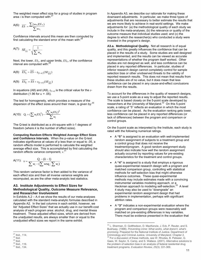
In Appendix A3, we describe our rationale for making these downward adjustments. In particular, we make three types of adjustments that are necessary to better estimate the results that we are more likely to achieve in real-world settings. We make adjustments for: (a) the methodological quality of each study we include in the meta-analyses; (b) the relevance or quality of the outcome measure that individual studies used; and (c) the degree to which the researcher(s) who conducted a study were invested in the program’s design.

A3.a. Methodological Quality. Not all research is of equal quality, and this greatly influences the confidence that can be placed in the results of a study. Some studies are well designed and implemented, and the results can be viewed as accurate representations of whether the program itself worked. Other studies are not designed as well, and less confidence can be placed in any reported differences. In particular, studies of inferior research design cannot completely control for sample selection bias or other unobserved threats to the validity of reported research results. This does not mean that results from these studies are of no value, but it does mean that less confidence can be placed in any cause-and-effect conclusions drawn from the results. To account for the differences in the quality of research designs, we use a 5-point scale as a way to adjust the reported results. The scale is based closely on the 5-point scale developed by researchers at the University of Maryland.32 On this 5-point scale, a rating of “5” reflects an evaluation in which the most confidence can be placed. As the evaluation ranking gets lower, less confidence can be placed in any reported differences (or lack of differences) between the program and comparison or control groups. On the 5-point scale as interpreted by the Institute, each study is rated with the following numerical ratings.

• A “5” is assigned to an evaluation with well-implemented random assignment of subjects to a treatment group and a control group that does not receive the treatment/program. A good random assignment study should also indicate how well the random assignment actually occurred by reporting values for pre-existing characteristics for the treatment and control groups.

• A “4” is assigned to a study that employs a rigorous quasi-experimental research design with a program and matched comparison group, controlling with statistical methods for self-selection bias that might otherwise influence outcomes. These quasi-experimental methods may include estimates made with a convincing instrumental variables modeling approach, or a Heckman approach to modeling self-selection.33 A level 4 study may also be used to “downgrade” an experimental random assignment design that had problems in implementation, perhaps with significant attrition rates.

• A “3” indicates a non-experimental evaluation where the program and comparison groups were reasonably well matched on pre-existing differences in key variables. There must be evidence presented in the evaluation that

32 L. Sherman, D. Gottfredson, D. MacKenzie, J. Eck, P. Reuter, and S. Bushway. (1998). Preventing crime: What works, what doesn't, what's promising. Prepared for the National Institute of Justice. Department of Criminology and Criminal Justice, University of Maryland. Chapter 2. 33 For a discussion of these methods, see W. Rhodes, B. Pelissier, G. Gaes, W. Saylor, S. Camp, and S. Wallace. (2001). Alternative solutions to the problem of selection bias in an analysis of federal residential drug treatment programs. Evaluation Review, 25(3): 331-369.

12

indicates few, if any, significant differences were observed in these salient pre-existing variables. Alternatively, if an evaluation employs sound multivariate statistical techniques (e.g., logistic regression) to control for pre-existing differences, and if the analysis is successfully completed, then a study with some differences in pre-existing variables can qualify as a level 3.

• A “2” involves a study with a program and matched comparison group where the two groups lack comparability on pre-existing variables and no attempt was made to control for these differences in the study.

• A “1” involves a study where no comparison group is utilized. Instead, the relationship between a program and an outcome, i.e., drug use, is analyzed before and after the program.

We do not use the results from program evaluations rated as a “1” on this scale, because they do not include a comparison group and, thus, no context to judge program effectiveness. We also regard evaluations with a rating of “2” as highly problematic and, as a result, do not consider their findings in the calculations of effect. In this study, we only considered evaluations that rated at least a 3 on this 5-point scale. An explicit adjustment factor is assigned to the results of individual effect sizes based on the Institute’s judgment concerning research design quality. This adjustment is critical and the only practical way to combine the results of a high quality study (e.g., a level 5 study) with those of lesser design quality (level 4 and level 3 studies). The specific adjustments made for these studies are based on our knowledge of research in other topic areas. For example, in criminal justice program evaluations, there is strong evidence that random assignment studies (i.e., level 5 studies) have, on average, smaller absolute effect sizes than weaker-designed studies.34 Thus, we use the following “default” adjustments to account for studies of different research design quality:

• A level 5 study carries a factor of 1.0 (that is, there is no discounting of the study’s evaluation outcomes).

• A level 4 study carries a factor of .75 (effect sizes discounted by 25 percent).

• A level 3 study carries a factor of .50 (effect sizes discounted by 50 percent).

• We do not include level 2 and level 1 studies in our analyses.

These factors are subjective to a degree; they are based on the Institute’s general impressions of the confidence that can be placed in the predictive power of evaluations of different quality.

34 M.W. Lipsey. (2003). Those confounded moderators in meta-analysis: Good, bad, and ugly. The Annals of the American Academy of Political and Social Science, 587(1): 69-81. Lipsey found that, for juvenile delinquency evaluations, random assignment studies produced effect sizes only 56 percent as large as nonrandom assignment studies.

The effect of the adjustment is to multiply the effect size for any study, ES'm, in equation (A3) by the appropriate research design factor. For example, if a study has an effect size of -.20 and it is deemed a level 4 study, then the -.20 effect size would be multiplied by .75 to produce a -.15 adjusted effect size for use in the benefit-cost analysis. A3.b. Adjusting Effect Sizes of Studies With Short-Term Follow-Up Periods. To account for the likelihood that the effects of treatment do not persist indefinitely for all subjects, we discount effect sizes, ESm, over time. The majority of studies coded report only short-term outcomes. Few of the studies provided outcomes beyond one year post-treatment and many reported outcomes only during or at the end of a treatment episode. Therefore, the unadjusted meta-analytic effect sizes reflect relatively short-term outcomes. To reflect the likelihood that the effects of a given treatment will decline over time, we built in a “decay” factor. In Appendix B, we discuss the methods by which we decay these effects. A3.c. Adjusting Effect Sizes for Research Involvement in the Program’s Design and Implementation. The purpose of the Institute’s work is to identify and evaluate programs that can make cost-beneficial improvements to Washington’s actual service delivery system. There is some evidence that programs closely controlled by researchers or program developers have better results than those that operate in “real world” administrative structures.35 In our evaluation of a real-world implementation of a research-based juvenile justice program in Washington, we found that the actual results were considerably lower than the results obtained when the intervention was conducted by the originators of the program.36 Therefore, we make an adjustment to effect sizes, ESm, to reflect this distinction. As a parameter for all studies deemed not to be “real world” trials, the Institute discounts ES'm by .5, although this can be modified on a study-by-study basis. A4. Meta-Analytic Results—Estimated Effect Sizes and Citations to Studies Used in the Analyses Exhibits A. 2, A.3, and A.4 provide technical meta-analytic results for the effect sizes computed for this analysis. Each table provides the unadjusted and adjusted effect sizes for EBT in each of the three program areas, and lists all of the studies included in each analysis. Exhibit A.5 lists the citations for all studies used in the meta-analyses. The meta-analytic results of the effects of EBT on disordered alcohol use are displayed in Exhibit A.2. The results for disordered drug use and mental illness are displayed in Exhibits A.3 and A.4, respectively.

35 Ibid. Lipsey found that, for juvenile delinquency evaluations, programs in routine practice (i.e., “real world” programs) produced effect sizes only 61 percent as large as research/demonstration projects. See also: A. Petrosino, and H. Soydan. (2005). The impact of program developers as evaluators on criminal recidivism: Results from meta-analyses of experimental and quasi-experimental research. Journal of Experimental Criminology, 1(4): 435-450. 36 R. Barnoski. (2004). Outcome evaluation of Washington State's research-based programs for juvenile offenders. Olympia: Washington State Institute for Public Policy, available at <http://www.wsipp.wa.gov/rptfiles/04-01-1201.pdf>.

13

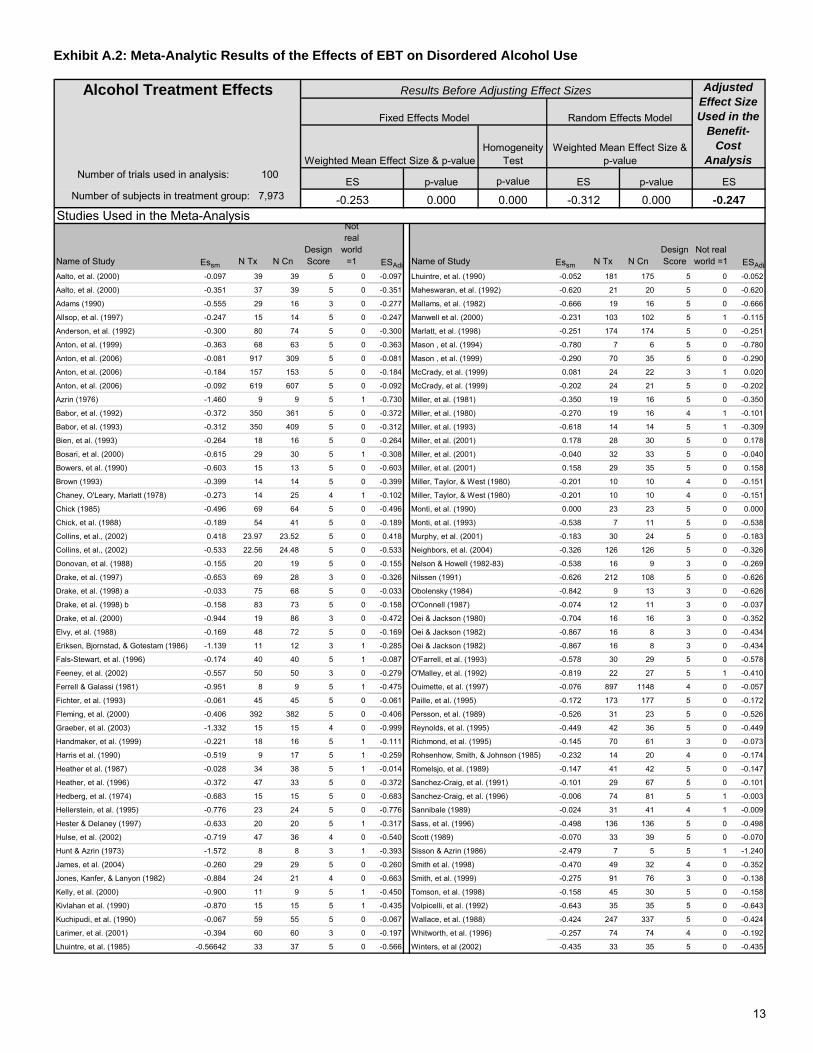
Exhibit A.2: Meta-Analytic Results of the Effects of EBT on Disordered Alcohol Use

p-value

0.000Studies Used in the Meta-Analysis

Name of Study Essm N Tx N CnDesign Score

Not real

world =1 ESAdj Name of Study Essm N Tx N Cn

Design Score

Not real world =1 ESAdj

Aalto, et al. (2000) -0.097 39 39 5 0 -0.097 Lhuintre, et al. (1990) -0.052 181 175 5 0 -0.052

Aalto, et al. (2000) -0.351 37 39 5 0 -0.351 Maheswaran, et al. (1992) -0.620 21 20 5 0 -0.620

Adams (1990) -0.555 29 16 3 0 -0.277 Mallams, et al. (1982) -0.666 19 16 5 0 -0.666

Allsop, et al. (1997) -0.247 15 14 5 0 -0.247 Manwell et al. (2000) -0.231 103 102 5 1 -0.115

Anderson, et al. (1992) -0.300 80 74 5 0 -0.300 Marlatt, et al. (1998) -0.251 174 174 5 0 -0.251

Anton, et al. (1999) -0.363 68 63 5 0 -0.363 Mason , et al. (1994) -0.780 7 6 5 0 -0.780

Anton, et al. (2006) -0.081 917 309 5 0 -0.081 Mason , et al. (1999) -0.290 70 35 5 0 -0.290

Anton, et al. (2006) -0.184 157 153 5 0 -0.184 McCrady, et al. (1999) 0.081 24 22 3 1 0.020

Anton, et al. (2006) -0.092 619 607 5 0 -0.092 McCrady, et al. (1999) -0.202 24 21 5 0 -0.202

Azrin (1976) -1.460 9 9 5 1 -0.730 Miller, et al. (1981) -0.350 19 16 5 0 -0.350

Babor, et al. (1992) -0.372 350 361 5 0 -0.372 Miller, et al. (1980) -0.270 19 16 4 1 -0.101

Babor, et al. (1993) -0.312 350 409 5 0 -0.312 Miller, et al. (1993) -0.618 14 14 5 1 -0.309

Bien, et al. (1993) -0.264 18 16 5 0 -0.264 Miller, et al. (2001) 0.178 28 30 5 0 0.178

Bosari, et al. (2000) -0.615 29 30 5 1 -0.308 Miller, et al. (2001) -0.040 32 33 5 0 -0.040

Bowers, et al. (1990) -0.603 15 13 5 0 -0.603 Miller, et al. (2001) 0.158 29 35 5 0 0.158

Brown (1993) -0.399 14 14 5 0 -0.399 Miller, Taylor, & West (1980) -0.201 10 10 4 0 -0.151

Chaney, O'Leary, Marlatt (1978) -0.273 14 25 4 1 -0.102 Miller, Taylor, & West (1980) -0.201 10 10 4 0 -0.151

Chick (1985) -0.496 69 64 5 0 -0.496 Monti, et al. (1990) 0.000 23 23 5 0 0.000

Chick, et al. (1988) -0.189 54 41 5 0 -0.189 Monti, et al. (1993) -0.538 7 11 5 0 -0.538

Collins, et al., (2002) 0.418 23.97 23.52 5 0 0.418 Murphy, et al. (2001) -0.183 30 24 5 0 -0.183

Collins, et al., (2002) -0.533 22.56 24.48 5 0 -0.533 Neighbors, et al. (2004) -0.326 126 126 5 0 -0.326

Donovan, et al. (1988) -0.155 20 19 5 0 -0.155 Nelson & Howell (1982-83) -0.538 16 9 3 0 -0.269

Drake, et al. (1997) -0.653 69 28 3 0 -0.326 Nilssen (1991) -0.626 212 108 5 0 -0.626

Drake, et al. (1998) a -0.033 75 68 5 0 -0.033 Obolensky (1984) -0.842 9 13 3 0 -0.626

Drake, et al. (1998) b -0.158 83 73 5 0 -0.158 O'Connell (1987) -0.074 12 11 3 0 -0.037

Drake, et al. (2000) -0.944 19 86 3 0 -0.472 Oei & Jackson (1980) -0.704 16 16 3 0 -0.352

Elvy, et al. (1988) -0.169 48 72 5 0 -0.169 Oei & Jackson (1982) -0.867 16 8 3 0 -0.434

Eriksen, Bjornstad, & Gotestam (1986) -1.139 11 12 3 1 -0.285 Oei & Jackson (1982) -0.867 16 8 3 0 -0.434

Fals-Stewart, et al. (1996) -0.174 40 40 5 1 -0.087 O'Farrell, et al. (1993) -0.578 30 29 5 0 -0.578

Feeney, et al. (2002) -0.557 50 50 3 0 -0.279 O'Malley, et al. (1992) -0.819 22 27 5 1 -0.410

Ferrell & Galassi (1981) -0.951 8 9 5 1 -0.475 Ouimette, et al. (1997) -0.076 897 1148 4 0 -0.057

Fichter, et al. (1993) -0.061 45 45 5 0 -0.061 -0.172 173 177 5 0 -0.172

Fleming, et al. (2000) -0.406 392 382 5 0 -0.406 Persson, et al. (1989) -0.526 31 23 5 0 -0.526

Graeber, et al. (2003) -1.332 15 15 4 0 -0.999 Reynolds, et al. (1995) -0.449 42 36 5 0 -0.449

Handmaker, et al. (1999) -0.221 18 16 5 1 -0.111 Richmond, et al. (1995) -0.145 70 61 3 0 -0.073

Harris et al. (1990) -0.519 9 17 5 1 -0.259 Rohsenhow, Smith, & Johnson (1985) -0.232 14 20 4 0 -0.174

Heather et al. (1987) -0.028 34 38 5 1 -0.014 Romelsjo, et al. (1989) -0.147 41 42 5 0 -0.147

Heather, et al. (1996) -0.372 47 33 5 0 -0.372 Sanchez-Craig, et al. (1991) -0.101 29 67 5 0 -0.101

Hedberg, et al. (1974) -0.683 15 15 5 0 -0.683 Sanchez-Craig, et al. (1996) -0.006 74 81 5 1 -0.003

Hellerstein, et al. (1995) -0.776 23 24 5 0 -0.776 Sannibale (1989) -0.024 31 41 4 1 -0.009

Hester & Delaney (1997) -0.633 20 20 5 1 -0.317 Sass, et al. (1996) -0.498 136 136 5 0 -0.498

Hulse, et al. (2002) -0.719 47 36 4 0 -0.540 Scott (1989) -0.070 33 39 5 0 -0.070

Hunt & Azrin (1973) -1.572 8 8 3 1 -0.393 Sisson & Azrin (1986) -2.479 7 5 5 1 -1.240

James, et al. (2004) -0.260 29 29 5 0 -0.260 Smith et al. (1998) -0.470 49 32 4 0 -0.352

Jones, Kanfer, & Lanyon (1982) -0.884 24 21 4 0 -0.663 Smith, et al. (1999) -0.275 91 76 3 0 -0.138

Kelly, et al. (2000) -0.900 11 9 5 1 -0.450 Tomson, et al. (1998) -0.158 45 30 5 0 -0.158

Kivlahan et al. (1990) -0.870 15 15 5 1 -0.435 Volpicelli, et al. (1992) -0.643 35 35 5 0 -0.643

Kuchipudi, et al. (1990) -0.067 59 55 5 0 -0.067 Wallace, et al. (1988) -0.424 247 337 5 0 -0.424

Larimer, et al. (2001) -0.394 60 60 3 0 -0.197 Whitworth, et al. (1996) -0.257 74 74 4 0 -0.192

Lhuintre, et al. (1985) -0.56642 33 37 5 0 -0.566 Winters, et al (2002) -0.435 33 35 5 0 -0.435

p-value

Alcohol Treatment Effects

-0.247ES

-0.253 0.000 -0.312 0.000ES

Paille, et al. (1995)

Number of trials used in analysis: 100

Number of subjects in treatment group: 7,973p-valueES

Adjusted Effect Size Used in the

Benefit-Cost

Analysis

Random Effects Model

Weighted Mean Effect Size & p-valueWeighted Mean Effect Size & p-value

Homogeneity Test

Results Before Adjusting Effect Sizes

Fixed Effects Model

14

Exhibit A.3: Meta-Analytic Results of the Effects of EBT on Disordered Drug Use

p-value0.000

Studies Used in the Meta-AnalysisName of Study Essm N Tx N Cn Score real ESAdj Name of Study Essm N Tx N Cn Score world =1 ESAdjAvants, et al. (2004) -0.232 108 112 5 0 -0.232 Johnson, et al. (1992) -0.491 90 60 5 0 -0.491

Azrin, et al. (1996) -0.651 37 37 3 1 -0.163 Johnson, et al. (1995) -0.641 90 60 5 0 -0.641

Azrin, et al.(1994) -0.714 15 11 4 1 -0.268 Johnson, et al. (2000) -0.487 55 55 5 0 -0.487

Baker, et al. (2001) -0.688 32 32 3 1 -0.172 Kavanagh, et al. (2004) -0.725 13 8 5 0 -0.725

Baker, et al. (2005) -0.472 74 74 4 1 -0.177 Ling, et al. (1998) -0.443 90 60 5 0 -0.443

Baker, et al. (2005) -0.494 66 74 4 1 -0.185 Margolin, et al. (2003) -0.383 45 45 5 0 -0.383

Bellack, et al. (2006) -0.680 61 49 5 1 -0.340 Marijuana Treatment Project (2004) -0.216 127 137 5 0 -0.216

Carroll, et al. (1991) -0.206 21 21 4 1 -0.077 Marijuana Treatment Project (2004) -0.610 132 137 5 0 -0.610

Carroll, et al. (1994) -0.461 52 45 4 1 -0.173 Milby, et al. (1996) -0.044 69 62 3 0 -0.022

Catalano, et al. (2002) -0.048 63 63 5 1 -0.024 Newman, et al. (1979) -0.827 50 50 5 0 -0.827

Cornish, et al. (1997) -0.577 34 17 5 0 -0.577 Petry & Martin (2002) -1.498 19 23 5 0 -1.498

Ctrits-Christoph, et al. (1999) -0.237 121 123 4 0 -0.178 Petry, et al. ( 2000) -0.772 19 23 5 0 -0.772

Dole, et al. (1969) -2.051 12 16 5 1 -1.026 Piotrowski, et al. (1999) 0.000 51 51 5 0 0.000

Drake, et al. (1997) -0.113 78 29 3 0 -0.056 Rawson, et al. (1995) -0.122 41 44 5 0 -0.122

Drake, et al. (1998)a -0.178 45 40 5 0 -0.178 Schottenfeld, et al. (1997) -0.291 30 29 5 0 -0.291

Drake, et al. (1998)b -0.124 45 40 5 0 -0.124 Silverman, et al., (1996) -0.534 15 15 4 0 -0.401

Drake, et al. (2000) -0.687 11 54 3 0 -0.344 Silverman, et al., (1998) -1.554 36 15 4 0 -1.165

Fudala, et al. (2003) -0.421 214 109 5 0 -0.421 Stephens, et al. (2000) -0.598 117 86 5 0 -0.598

Gronbladh, et al. (1989) -0.896 17 17 4 0 -0.672 Stephens, et al. (2000) -0.497 88 86 5 0 -0.497

Higgins, et al. (2000) -0.360 36 34 5 1 -0.180 Strain, et al. (1993) -0.329 84 81 5 0 -0.329

Humphreys, et al., (1999) -0.189 897 1148 4 0 -0.142 Vanichseni, et al. (1991) -0.511 120 120 5 0 -0.511

James, et al. (2004) -0.868 29 29 5 0 -0.868 Woody, et al. (1995) -0.463 57 27 3 1 -0.116

0.000 -0.355



Benefit-Cost

Analysis

p-value ESNumber of subjects in treatment group: 3,506 -0.360 0.000 -0.451

Treatment forDisordered Drug Use


Fixed Effects Model

Weighted Mean Effect Size & p-valueHomogeneity

TestWeighted Mean Effect Size &

p-valueNumber of trials used in analysis: 44

ES p-value ES

15

A.4: Meta-Analytic Results of the Effects of EBT on Mental Illness Our benefit-cost analysis focused on serious mental illness: non-affective psychosis (including schizophrenia), bipolar disorder and severe forms of panic disorder, and depression. Because studies rarely indicated the severity of subjects’ mental disorders in the studies, our analysis included all programs for depression, and we estimated effects for panic disorder based on studies for treatments of anxiety disorders. To derive a single effect size for mental illness treatments, we first calculated effect sizes for four categories of mental illness: non-affective psychosis, bipolar, anxiety, and major depressive disorders. After weighting according to prevalence among the populations with serious mental illness, we combined the separate effect sizes into a single average (see the following table).

Weight ES Std ErrSchizophrenia (Non-affective psychosis) 0.079 -0.323 0.029Bipolar disorder 0.410 -0.382 0.048Anxiety disorders 0.191 -0.404 0.045Major Depressive Disorder 0.321 -0.280 0.061

All Mental Illness 1.000 -0.360 0.047

Disorder

Adjusted ES for Benefit-Cost Analysis

Note: Relative prevalence was based on incidence of serious major depression, serious panic disorder, and bipolar I and II reported from the National Comorbidity Survey Replication37 and non-affective psychosis as reported in the National Comorbidity Survey.38

p-value-0.549

Studies Used in the Meta-Analysis


Not real


Design Score


Burgess, et al.(2001) -0.300 413 412 5 0 -0.300 Rendell, et al. (2003) -0.524 54 56 5 0 -0.524

Macritchie, et al. (2003) -0.512 155 161 5 0 -0.512 Rendell, et al. (2003) -0.454 220 114 5 0 -0.454

Rendell, et al. (2003) -0.426 70 66 5 0 -0.426 Weiss, et al. (2000) -0.200 21 24 3 1 -0.050


Benefit-Cost

Analysis

Fixed Effects Model Random Effects Model

ES

Treatments for Bipolar Disorder


p-value



p-value

ESNumber of subjects in treatment group: 933 -0.386 0.000 na na -0.382

Number of trials used in analysis: 6 ES p-value

p-value0.018



Not real


Design Score


Browne, et al. (2002) 0.045 212 196 4 0 0.033 Shea, et al (1992) -0.194 59 62 5 0 -0.194

Fava, et al. (1998) -0.513 20 20 5 0 -0.513 Shea, et al (1992) -0.008 61 62 5 0 -0.008

Lima, et al. (2006) -0.434 206 179 5 0 -0.434 Simons, et al. (1986) -0.610 36 16 3 0 -0.305

Lima, et al. (2006) -0.528 143 155 5 0 -0.528 Tuunainen, et al. (2004) -0.060 39 32 5 0 -0.060

Lima, et al. (2006) -0.366 295 305 5 0 -0.366 Ward, et al., (2000) -0.185 63 67 5 0 -0.185

Moncrieff, et al. (2004) -0.325 395 355 5 0 -0.325 Wijkstra, et al. (2005) -0.430 48 101 5 0 -0.430

Reynolds, et al. (2006) -0.493 25 28 5 0 -0.493 Wijkstra, et al. (2005) -0.368 100 101 5 0 -0.368

Reynolds, et al. (2006) 0.623 25 29 5 0 -0.623 Wijkstra, et al. (2005) -0.786 22 17 5 0 -0.786

0.000 -0.315Number of trials used in analysis: 16 ES

Number of subjects in treatment group: 1,479 -0.314 0.000 -0.323p-value ES



p-value

Treatments for Depression Results Before Adjusting Effect Sizes Adjusted Effect Size Used in the

Benefit-Cost

Analysis


p-value ES

37 R.C. Kessler, W.T. Chiu, O. Demler et al. (2005), Prevalence, severity, and comorbidity of 12-month DSM-IV disorders in the National Comorbidity Survey Replication. Archives of General Psychiatry, 62(6):617-627. 38 R.C. Kessler, K.A. McGonagle, S. Zhao et al. (1994). Lifetime and 12-month prevalence of DSM-III-R Psychiatric Disorders in the United States. Archives of General Psychiatry, 51: 8-19.

16

p-value0.000



Not real


Design Score


Barlow, et al. (1989) -1.394 10 15 5 0 -1.394 Cordioli, et al. (2003) -1.201 23 24 5 0 -1.201

Barlow, et al. (1989) -0.858 15 15 5 0 -0.858 Dugas, et al. (2003) -1.364 25 37 5 1 -0.682

Barlow, et al. (1989) -0.938 16 15 5 0 -0.938 Durham, et al. (1994) -0.710 35 29 4 1 -0.266

Barlow, et al. (1984) -1.205 10 10 5 0 -1.205 Kapczinski (2003) -0.378 277 280 5 0 -0.378

Barlow, et al. (2000) -0.553 60 22 5 0 -0.553 Ladouceur, et al. (2000) -1.571 14 12 5 1 -0.785

Barlow, et al., (1992) -1.588 24 10 3 1 -0.397 Lindsay, et al. (1987) -1.200 10 10 5 1 -0.600

Beck, et al. (1992) -0.507 17 16 3 1 -0.127 Linehan, et al. (1999) -0.289 12 16 5 1 -0.144

Bisson & Andrew (2005) -0.375 79 77 4 0 -0.281 Marks, et al., (1993) -0.909 23 17 3 0 -0.454

Bisson & Andrew (2005) -0.426 266 187 5 0 -0.426 Mortberg, et al. (2005) -1.005 12 12 5 1 -0.502

Bisson & Andrew (2005) -1.006 44 42 5 0 -1.006 Pittler, et al. (2003) -0.201 197 183 5 0 -0.201

Blomhoff, et al. (2001) -0.256 91 88 5 0 -0.256 Stein, et al. (2000) -0.146 1872 1824 5 0 -0.146

Blomhoff, et al. (2001) -0.508 88 88 5 0 -0.508 Stein, et al (2006 ) -0.177 1270 1237 5 0 -0.177

Borkovec & Costello (1993) -0.342 18 20 4 1 -0.128 White & Keenan (1992) -0.119 26 10 3 1 -0.030

Borkovec & Mathews (1988) -0.410 10 10 5 0 -0.410 White & Keenan (1992) -0.354 31 10 3 1 -0.089

Borkovec, et al (1987) -0.367 16 14 4 0 -0.275 White & Keenan (1992) -0.318 31 10 3 1 -0.080

Butler, et al., (1991) -1.203 19 19 5 0 -1.203


Benefit-Cost

Analysis




p-valuep-value ES

Treatments for Anxiety Disorders


p-value ESNumber of subjects in treatment group: 4,641 -0.256 0.000 -0.563 0.000 -0.404

Number of trials used in analysis: 31 ES

p-value

0.000Studies Used in the Meta-AnalysisName of Study Essm N Tx N Cn Score real ESAdj Name of Study Essm N Tx N Cn Score world =1 ESAdjAber-Wistedt, et al. (1995) -0.557 20 20 5 0 -0.557 Haddock, et al., (2006) -0.542 15 14 5 1 -0.271

Barrowclough, et al. (2001) -0.633 17 15 5 1 -0.317 Hoult, et al. (1984) -0.541 26 25 5 0 -0.541

Bigelow, et al. (1991) -0.812 15 7 3 0 -0.406 James, et al. (2004) -0.60129 29.000 29 5 0 -0.60129

Bond, et al. (1988) -0.460 84 83 5 0 -0.460 Joy, et al. (2004) -0.202 228 237 5 0 -0.202

Bond, et al. (1988) -0.516 84 83 5 0 -0.516 Lehman, et al. (1994) -0.201 359 302 3 0 -0.101

Bond, et al. (1990) -0.743 42 40 5 0 -0.743 Lehman, et al. (1997) -0.354 77 75 5 0 -0.354

Bond, et al. (1991) -1.098 30 10 3 1 -0.274 Lewis, et al. (2005) -0.308 40 38 5 0 -0.308

Bond, et al. (1995) -0.502 39 35 3 0 -0.251 Macias, et al. (1994) -0.802 19 18 4 0 -0.602

Bush. et al. (1990) -0.832 14 14 5 0 -0.832 Marques (2004) -0.266 208 207 5 0 -0.266

Curtis, et al. (1996) -0.023 147 145 5 0 -0.023 McFarlane (2002) -0.514 27 14 5 0 -0.514

Chandler, et al. (1996) -0.450 115 108 5 0 -0.450 McFarlane (2002) -0.291 50 50 5 0 -0.291

Chandler, et al. (1997) -0.431 105 105 3 1 -0.108 McFarlane (2002) -0.297 34 34 5 0 -0.297

Chandler, et al. (1997) -0.431 105 105 3 1 -0.108 McFarlane, et al. (1995) -0.289 83 89 5 0 -0.289

Drake et al. (1998) -0.017 105 98 5 0 -0.017 McFarlane, et al. (2000) 0.585 37 32 5 0 0.585

Drake, et al. (1996) -0.660 39 35 3 0 -0.330 Morse, et al. (1997) -0.421 90 45 4 0 -0.316

Drake, et al. (1999) -1.166 74 76 3 1 -0.292 Mota Neto, et al. (2002) -0.590 159 83 5 0 -0.590

Dyck, et al. (2002) -0.428 55 51 5 0 -0.428 Quinlivan, et al. (1995) -0.510 30 30 5 0 -0.510

Dyck, et al. (2002) -0.150 56 150 3 0 -0.075 Shern, et al. (2000) -0.453 91 77 5 0 -0.453

El-Sayeh & Morganti (2006) -0.452 155 155 5 0 -0.452 Test, et al. (1980) -0.321 54 57 3 0 -0.160

Essock, et al. (1995) -0.503 58 50 5 0 -0.503 Test, et al. (1991) -0.680 75 47 5 0 -0.680

Fekete, et al. (1998) -0.534 58 50 3 0 -0.267 Tharyan, et al. (2005) -0.363 214 178 5 0 -0.363

Ford, et al. (1996) -0.375 47 47 3 0 -0.188 Thornley, et al. (2003) -0.229 264 248 5 0 -0.229

Gervey, et al. (1994) -1.584 17 17 3 1 -0.396 Wilson, et al. (1995) -0.511 26 33 5 0 -0.511

Goering, et al. (1988) -0.189 82 82 3 0 -0.094 Wood, et al. (1995) -0.753 32 32 3 0 -0.376

Gold, et al. (2005) -0.678 99 81 5 0 -0.678

Note: Treatments in Assertive Community Treatment were predominantly schizophrenics but included people with other serious mental illness.

p-valueES


ESNumber of subjects in treatment group: 3,926 -0.370 0.000 -0.423 0.000 -0.324

Number of trials used in analysis: 49 ES p-value


Benefit-Cost

Analysis




p-value

Fixed Effects Model

Treatments for Non-Affective Psychosis (Including

Schizophrenia)

17

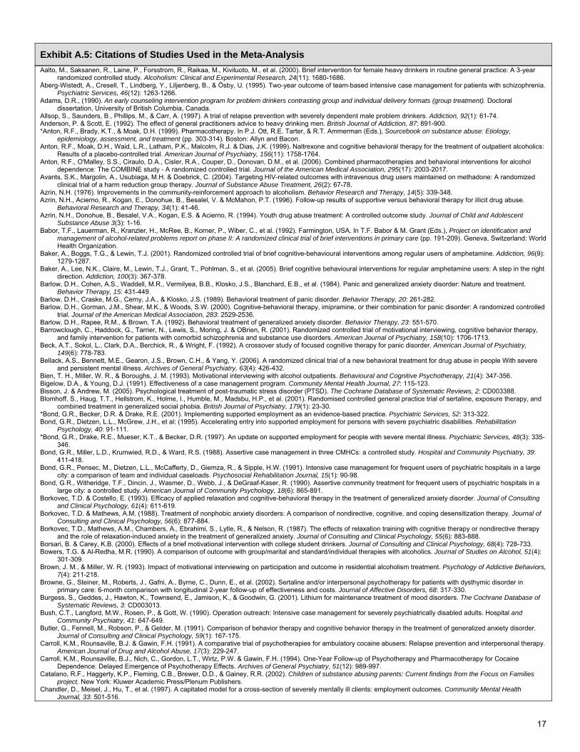
Exhibit A.5: Citations of Studies Used in the Meta-Analysis

Aalto, M., Saksanen, R., Laine, P., Forsstrom, R., Raikaa, M., Kiviluoto, M., et al. (2000). Brief intervention for female heavy drinkers in routine general practice: A 3-year randomized controlled study. Alcoholism: Clinical and Experimental Research, 24(11): 1680-1686.

Åberg-Wistedt, A., Cresell, T., Lindberg, Y., Liljenberg, B., & Ösby, U. (1995). Two-year outcome of team-based intensive case management for patients with schizophrenia. Psychiatric Services, 46(12): 1263-1266.

Adams, D.R., (1990). An early counseling intervention program for problem drinkers contrasting group and individual delivery formats (group treatment). Doctoral dissertation, University of British Columbia, Canada.

Allsop, S., Saunders, B., Phillips, M., & Carr, A. (1997). A trial of relapse prevention with severely dependent male problem drinkers. Addiction, 92(1): 61-74. Anderson, P. & Scott, E. (1992). The effect of general practitioners advice to heavy drinking men. British Journal of Addiction, 87: 891-900. *Anton, R.F., Brady, K.T., & Moak, D.H. (1999). Pharmacotherapy. In P.J. Ott, R.E. Tarter, & R.T. Ammerman (Eds.), Sourcebook on substance abuse: Etiology,

epidemiology, assessment, and treatment (pp. 303-314). Boston: Allyn and Bacon. Anton, R.F., Moak, D.H., Waid, L.R., Latham, P.K., Malcolm, R.J. & Dias, J.K. (1999). Naltrexone and cognitive behavioral therapy for the treatment of outpatient alcoholics:

Results of a placebo-controlled trial. American Journal of Psychiatry, 156(11): 1758-1764. Anton, R.F., O'Malley, S.S., Ciraulo, D.A., Cisler, R.A., Couper, D., Donovan, D.M., et al. (2006). Combined pharmacotherapies and behavioral interventions for alcohol

dependence: The COMBINE study - A randomized controlled trial. Journal of the American Medical Association, 295(17): 2003-2017. Avants, S.K., Margolin, A., Usubiaga, M.H. & Doebrick, C. (2004). Targeting HIV-related outcomes with intravenous drug users maintained on methadone: A randomized

clinical trial of a harm reduction group therapy. Journal of Substance Abuse Treatment, 26(2): 67-78. Azrin, N.H. (1976). Improvements in the community-reinforcement approach to alcoholism. Behavior Research and Therapy, 14(5): 339-348. Azrin, N.H., Acierno, R., Kogan, E., Donohue, B., Besalel, V. & McMahon, P.T. (1996). Follow-up results of supportive versus behavioral therapy for illicit drug abuse.

Behavioral Research and Therapy, 34(1): 41-46. Azrin, N.H., Donohue, B., Besalel, V.A., Kogan, E.S. & Acierno, R. (1994). Youth drug abuse treatment: A controlled outcome study. Journal of Child and Adolescent

Substance Abuse 3(3): 1-16. Babor, T.F., Lauerman, R., Kranzler, H., McRee, B., Korner, P., Wiber, C., et al. (1992). Farmington, USA. In T.F. Babor & M. Grant (Eds.), Project on identification and

management of alcohol-related problems report on phase II: A randomized clinical trial of brief interventions in primary care (pp. 191-209). Geneva, Switzerland: World Health Organization.

Baker, A., Boggs, T.G., & Lewin, T.J. (2001). Randomized controlled trial of brief cognitive-behavioural interventions among regular users of amphetamine. Addiction, 96(9): 1279-1287.

Baker, A., Lee, N.K., Claire, M., Lewin, T.J., Grant, T., Pohlman, S., et al. (2005). Brief cognitive behavioural interventions for regular amphetamine users: A step in the right direction. Addiction, 100(3): 367-378.

Barlow, D.H., Cohen, A.S., Waddell, M.R., Vermilyea, B.B., Klosko, J.S., Blanchard, E.B., et al. (1984). Panic and generalized anxiety disorder: Nature and treatment. Behavior Therapy, 15: 431-449.

Barlow, D.H., Craske, M.G., Cerny, J.A., & Klosko, J.S. (1989). Behavioral treatment of panic disorder. Behavior Therapy, 20: 261-282. Barlow, D.H., Gorman, J.M., Shear, M.K., & Woods, S.W. (2000). Cognitive-behavioral therapy, imipramine, or their combination for panic disorder: A randomized controlled

trial. Journal of the American Medical Association, 283: 2529-2536. Barlow, D.H., Rapee, R.M., & Brown, T.A. (1992). Behavioral treatment of generalized anxiety disorder. Behavior Therapy, 23: 551-570. Barrowclough, C., Haddock, G., Tarrier, N., Lewis, S., Moring, J. & OBrien, R. (2001). Randomized controlled trial of motivational interviewing, cognitive behavior therapy,

and family intervention for patients with comorbid schizophrenia and substance use disorders. American Journal of Psychiatry, 158(10): 1706-1713. Beck, A.T., Sokol, L., Clark, D.A., Berchick, R., & Wright, F. (1992). A crossover study of focused cognitive therapy for panic disorder. American Journal of Psychiatry,

149(6): 778-783. Bellack, A.S., Bennett, M.E., Gearon, J.S., Brown, C.H., & Yang, Y. (2006). A randomized clinical trial of a new behavioral treatment for drug abuse in people With severe

and persistent mental illness. Archives of General Psychiatry, 63(4): 426-432. Bien, T. H., Miller, W. R., & Boroughs, J. M. (1993). Motivational interviewing with alcohol outpatients. Behavioural and Cognitive Psychotherapy, 21(4): 347-356. Bigelow, D.A., & Young, D.J. (1991). Effectiveness of a case management program. Community Mental Health Journal, 27: 115-123. Bisson, J. & Andrew, M. (2005). Psychological treatment of post-traumatic stress disorder (PTSD). The Cochrane Database of Systematic Reviews, 2: CD003388. Blomhoff, S., Haug, T.T., Hellstrom, K., Holme, I., Humble, M., Madsbu, H.P., et al. (2001). Randomised controlled general practice trial of sertaline, exposure therapy, and

combined treatment in generalized social phobia. British Journal of Psychiatry, 179(1): 23-30. *Bond, G.R., Becker, D.R. & Drake, R.E. (2001). Implementing supported employment as an evidence-based practice. Psychiatric Services, 52: 313-322. Bond, G.R., Dietzen, L.L., McGrew, J.H., et al: (1995). Accelerating entry into supported employment for persons with severe psychiatric disabilities. Rehabilitation

Psychology, 40: 91-111. *Bond, G.R., Drake, R.E., Mueser, K.T., & Becker, D.R. (1997). An update on supported employment for people with severe mental illness. Psychiatric Services, 48(3): 335-

346. Bond, G.R., Miller, L.D., Krumwied, R.D., & Ward, R.S. (1988). Assertive case management in three CMHCs: a controlled study. Hospital and Community Psychiatry, 39:

411-418. Bond, G.R., Pensec, M., Dietzen, L.L., McCafferty, D., Giemza, R., & Sipple, H.W. (1991). Intensive case management for frequent users of psychiatric hospitals in a large

city: a comparison of team and individual caseloads. Psychosocial Rehabilitation Journal, 15(1): 90-98. Bond, G.R., Witheridge, T.F., Dincin, J., Wasmer, D., Webb, J., & DeGraaf-Kaser, R. (1990). Assertive community treatment for frequent users of psychiatric hospitals in a

large city: a controlled study. American Journal of Community Psychology, 18(6): 865-891. Borkovec, T.D. & Costello, E. (1993). Efficacy of applied relaxation and cognitive-behavioral therapy in the treatment of generalized anxiety disorder. Journal of Consulting

and Clinical Psychology, 61(4): 611-619. Borkovec, T.D. & Mathews, A.M. (1988). Treatment of nonphobic anxiety disorders: A comparison of nondirective, cognitive, and coping desensitization therapy. Journal of

Consulting and Clinical Psychology, 56(6): 877-884. Borkovec, T.D., Mathews, A.M., Chambers, A., Ebrahimi, S., Lytle, R., & Nelson, R. (1987). The effects of relaxation training with cognitive therapy or nondirective therapy

and the role of relaxation-induced anxiety in the treatment of generalized anxiety. Journal of Consulting and Clinical Psychology, 55(6): 883-888. Borsari, B. & Carey, K.B. (2000). Effects of a brief motivational intervention with college student drinkers. Journal of Consulting and Clinical Psychology, 68(4): 728-733. Bowers, T.G. & Al-Redha, M.R. (1990). A comparison of outcome with group/marital and standard/individual therapies with alcoholics. Journal of Studies on Alcohol, 51(4):

301-309. Brown, J. M., & Miller, W. R. (1993). Impact of motivational interviewing on participation and outcome in residential alcoholism treatment. Psychology of Addictive Behaviors,

7(4): 211-218. Browne, G., Steiner, M., Roberts, J., Gafni, A., Byrne, C., Dunn, E., et al. (2002). Sertaline and/or interpersonal psychotherapy for patients with dysthymic disorder in

primary care: 6-month comparison with longitudinal 2-year follow-up of effectiveness and costs. Journal of Affective Disorders, 68: 317-330. Burgess, S., Geddes, J., Hawton, K., Townsend, E., Jamison, K., & Goodwin, G. (2001). Lithium for maintenance treatment of mood disorders. The Cochrane Database of

Systematic Reviews, 3: CD003013. Bush, C.T., Langford, M.W., Rosen, P., & Gott, W. (1990). Operation outreach: Intensive case management for severely psychiatrically disabled adults. Hospital and

Community Psychiatry, 41: 647-649. Butler, G., Fennell, M., Robson, P., & Gelder, M. (1991). Comparison of behavior therapy and cognitive behavior therapy in the treatment of generalized anxiety disorder.

Journal of Consulting and Clinical Psychology, 59(1): 167-175. Carroll, K.M., Rounsaville, B.J. & Gawin, F.H. (1991). A comparative trial of psychotherapies for ambulatory cocaine abusers: Relapse prevention and interpersonal therapy.

American Journal of Drug and Alcohol Abuse, 17(3): 229-247. Carroll, K.M., Rounsaville, B.J., Nich, C., Gordon, L.T., Wirtz, P.W. & Gawin, F.H. (1994). One-Year Follow-up of Psychotherapy and Pharmacotherapy for Cocaine

Dependence: Delayed Emergence of Psychotherapy Effects. Archives of General Psychiatry, 51(12): 989-997. Catalano, R.F., Haggerty, K.P., Fleming, C.B., Brewer, D.D., & Gainey, R.R. (2002). Children of substance abusing parents: Current findings from the Focus on Families

project. New York: Kluwer Academic Press/Plenum Publishers. Chandler, D., Meisel, J., Hu, T., et al. (1997). A capitated model for a cross-section of severely mentally ill clients: employment outcomes. Community Mental Health

Journal, 33: 501-516.

18

Exhibit A.5: Citations of Studies Used in the Meta-Analysis, continued

Chandler, D., Meisel, J., McGowen, M., Mintz, J., & Madison, K. (1996). Client outcomes in two model capitated integrated service agencies. Psychiatric Services, 47(1): 175-180.

Chaney, E.F., OLeary, M.R. & Marlatt, A.G. (1978). Skill training with alcoholics. Journal of Consulting and Clinical Psychology, 46: 1092-1104. Chick, J., Lloyd, G. & Crombie, E. (1985). Counseling problem drinkers in medical wards: A controlled study. British Medical Journal, 290: 965-967. Chick, J., Ritson, B., Connaughton, J., Stewart, A., & Chick, J. (1988). Advice versus extended treatment for alcoholism: A controlled trial. British Journal of Addiction, 83(2):

159-170. Collins, S.E., Carey, K.B., & Sliwinski, M.J. (2002). Mailed personalized normative feedback as a brief intervention for at-risk college drinkers. Journal of Studies on Alcohol,

63(5): 559-567. Cordioli, A.V., Heldt, E., Bochi, D.B., Margis, R., de Sousa, M.B., Tonello, J.F., et al. (2003). Cognitive-behavioral group therapy in obsessive-compulsive disorder: a

randomized clinical trial. Psychotherapy and Psychosomatics, 72(4): 211-6. Cornish, J.W., Metzger, D., Woody, G.E., Wilson, D., McLellan, A.T., Vandergrift, B., et al. (1997). Naltrexone pharmacotherapy for opioid dependent federal probationers.

Journal of Substance Abuse Treatment, 14(6): 529-534. Crits-Christoph, P., Siqueland, L., Blaine, J., Frank, A., Luborsky, L. & Onken, L.S. (1999). Psychosocial treatments for cocaine dependence: National institute on drug

abuse collaborative cocaine treatment study. Archives of General Psychiatry, 56(6): 493-502. Curtis, J.L., Millman, E.J., Struening, E., et al. (1996). Deaths among former psychiatric inpatients in an outreach case management program. Psychiatric Services, 47(4):

398-402. Dole, V.P., Robinson, J.W., Orraca, J., Towns, E., Searcy, P., & Caine, E. (1969). Methadone treatment of randomly selected criminal addicts. New England Journal of

Medicine, 280(25): 1372-1375. Donovan, D.M. & Ito, J.R. (1988). Cognitive behavioral relapse prevention strategies and aftercare in alcoholism rehabilitation. Psychology of Addictive Behaviors, 2(2): 74. Drake, R.E., McHugo, G.J., Bebout, R.R., Becker, D.R., Harris, M., Bond, G.R., et al. (1999). A Randomized Clinical Trial of Supported Employment for Inner-city Patients With Severe Mental Disorders. Archives of General Psychiatry, 56(7): 627-633. Drake, R.E., McHugo, G.J., Becker, D.R., Anthony, W.A., & Clark, R.E. (1996). The New Hampshire study of supported employment for people with severe mental illness.

Journal of Consulting and Clinical Psychology, 64(2): 391-39. Drake, R.E., McHugo, G.J., Clark, R.E., et al: (1998a). Assertive community treatment for patients with co-occurring severe mental illness and substance use disorder: a

clinical trial. American Journal of Orthopsychiatry, 68(2): 201-215. Drake, R.E., Mercer-McFadden, C., Mueser, K.T., McHugo, G.J. & Bond, G.R. (1998b). Review of integrated mental health and substance abuse treatment for patients With

dual disorders. Schizophrenia Bulletin, 24(4): 589-608. *Drake, R.E., Mueser, K.T., Brunette, M.F., & McHugo, G.J. (2004). A review of treatments for people with severe mental illnesses and co-occurring substance use

disorders. Psychiatric Rehabilitation Journal, 27(4): 360-374. Drake, R.E., Xie, H., McHugo, G.J. & Green, A.I. (2000). The effects of clozapine on alcohol and drug use disorders among patients With schizophrenia. Schizophrenia

Bulletin, 26(2): 441-449. Drake, R.E., Yovetich, N.A., Bebout, R.R., Harris, M. & McHugo, G.J. (1997). Integrated treatment for dually diagnosed homeless Adults. Journal of Nervous and Mental

Disease, 185(5): 298-305. Dugas, M.J., Ladouceur, R., Leger, E., Freeston, M.H., Langlois, F., Provencher, M.D., et al. (2003). Group cognitive-behavioral therapy for generalized anxiety disorder:

treatment outcome and long-term follow-up. Journal of Consulting and Clinical Psychology, 71(4): 821-825. Durham, R.C., Murphy, T. Allan, T., Richard, K., Treliving, L. R., & Fenton, G.W. (1994). Cognitive therapy, analytic psychotherapy and anxiety management training for

generalized anxiety disorder. British Journal of Psychiatry, 165: 315-323. Dyck, D.G., Hendryx, M.S., Short, R.A., Voss, W.D., & McFarlane, W.R. (2002). Service use among patients with schizophrenia in psychoeducational multiple-family group

treatment. Psychiatric Services, 53(6): 749-754. El-Sayeh, H.G. & Morganti, C. (2006). Aripiprazole for schizophrenia. The Cochrane Database of Systematic Reviews, 2: CD004578. Elvy, G.A., Wells, J.E. & Baird, K.A. (1988). Attempted referral as intervention for problem drinking in the general hospital. British Journal of Addiction, 83(1): 83-89. Eriksen, L., Björnstad, S., & Götestam, K. G. (1986). Social skills training in groups for alcoholics: One-year treatment outcome for groups and individuals. Addictive

Behaviors, 11(3): 309-330. Essock, S.M., & Kontos, N. (1995). Implementing assertive community treatment teams. Psychiatric Services, 46(7): 679-683. Fals-Stewart, W., Birchler, G.R., & Ofarrell, T.J. (1996). Behavioral couples therapy for male substance-abusing patients: Effects on relationship adjustment and drug-using

behavior. Journal of Consulting and Clinical Psychology, 64(5): 959-972. Fava, G.A., Rafanelli, C., Grandi, S., Canestrari, R., & Morphy, M.A. (1998) Six-year outcomes for cognitive behavioral treatment of residual symptoms in major depression.

The American Journal of Psychiatry, 155(10): 1443-1445. Feeney, G., Young, R., Connor, J., Tucker, J., & McPherson, A. (2002). Cognitive behaviour therapy combined with the relapse-prevention medication acamprosate: are

short-term treatment outcomes for alcohol dependence improved? The Australian and New Zealand Journal of Psychiatry, 36(5): 622-628. Fekete, D.M., Bond, G.R., McDonel, E.C., Salyers, M.P., Chen, A., & Miller, L. (1998). Rural assertive community treatment: a field experiment. Psychiatric Rehabilitation

Journal, 21(4): 371-379. Ferrell, W. L., & Galassi, J. P. (1981). Assertion training and human relations training in the treatment of chronic alcoholics. International Journal of the Addictions, 16(5):

959-968. Fichter, M.M., & Frick, U. (1993). The key relative’s impact on treatment and course of alcoholism. European Archives of Psychiatry and Clinical Neuroscience, 243(2): 87-94.Fleming, M., Mundt, M.P., French, M.T., Manwell, L.B., Stauffacher, E.A., & Barry, K.L. (2000). Benefit-cost analysis of brief physician advice with problem drinkers in

primary care settings. Medical Care, 38(1): 7-18. Ford, R., Ryan, P., & Norton, P., et al. (1996). Does intensive case management work? Clinical, social, and quality of life outcomes from a controlled study. Journal of

Mental Health, 5(4): 361-368. Fudala, P.J., Bridge, T.P., Herbert, S., Williford, W.O., Chiang, C.N., Jones, K., et al. (2003). Office-based treatment of opiate addiction with a sublingual-tablet formulation

of buprenorphine and naloxone. New England Journal of Medicine, 349(10): 949-958. Gervey, R. & Bedell, J.R. (1994). Supported employment in vocational rehabilitation. In J.R. Bedell (Ed.), Psychological Assessment and Treatment of Persons With Severe

Mental Disorders (pp. 151-175). Washington, DC, Taylor & Francis. Goering, P.N., Farkas, M., Wasylenki, D., et al. (1988). Improved functioning for case management clients. Psychosocial Rehabilitation Journal, 12(1): 3-17. Gold, C., Heldal, T.O., Dahle, T., & Wigram, T. (2005). Music therapy for schizophrenia or schizophrenia-like illnesses. The Cochrane Database of Systematic Reviews, 2:

CD004025. Graber, R.A. & Willer, W.R. (1988). Abstinence or controlled drinking goals for problem drinkers: A randomized clinical trial. Psychology of Addictive Behaviors, 2(1): 20-33. Gronbladh, L. & Gunne, L. (1989). Methadone-assisted rehabilitation of Swedish heroin addicts. Drug and Alcohol Dependence, 24(1): 31-37. Haddock, G., Barrowclough, C., Tarrier, N., Moring, J., O'Brien, R., Schofield, N., et al. (2006). Cognitive-behavioural therapy and motivational intervention for schizophrenia

and substance misuse: 18-month outcomes of a randomized controlled trial. British Journal of Psychiatry, 183: 418-426. Handmaker-Sheehy, N., Miller, W.R., & Manicke, M. (1999). Findings of a pilot study of motivational interviewing with pregnant drinkers. Journal of Studies on Alcohol,

62(2): 285-287. Harris, K.B. & Miller, W.R. (1990). Behavioral self-control training for problem drinkers: Mechanisms of efficacy. Psychology of Addictive Behaviors, 4(2): 82-90. Heather, N. (1996). The public health and brief interventions for excessive alcohol consumption: The British experience. Addictive Behaviors, 21(6): 857. Heather, N., Campion, P.D., Neville, R.G. & Maccabe, D. (1987). Evaluation of a controlled drinking minimal intervention for problem drinkers in general practice (The

DRAMS Scheme). Journal of the Royal College of General Practitioners, 37(301): 358-363. Hedberg, A. G., & Campbell, L. M. (1974). A comparison of four behavioral treatment approaches to alcoholism. Journal of Behavior Therapy and Experimental Psychiatry,

5(3/4): 251-256. Hellerstein, D.J., Rosenthal, R.N. & Miner, C.R. (1995). Prospective study of integrated outpatient treatment for substance-abusing schizophrenic patients. American Journal

on Addictions, 4(1): 33-42. Hester, R.K. & Delaney, H.D. (1997). Behavioral self-control program for windows: Results of a controlled clinical trial. Journal of Consulting and Clinical Psychology, 65(4):

686-693. Higgins, S.T., Wong, C.J., Badter, G.J., Haug Ogden, D.E. & Dantona, R.L. (2000). Contingent reinforcement increases cocaine abstinence during outpatient treatment and

1 year of follow-up. Journal of Consulting and Clinical Psychology, 68(1): 64-72.

19


Hoult, J. & Reynolds, I. (1984). Schizophrenia: A comparative trial of community orientated and hospital orientated psychiatric care. Acta Psychiatrica Scandinavica, 69(5): 359-372.

Hulse, G.K. & Tait, R.J. (2002). Six-month outcomes associated with brief alcohol intervention for adult in-patients with psychiatric disorders. Drug and Alcohol Review, 21: 105-112.

Humphreys, K., Huebsch, P.D., Finney, J.W., & Moos, R.H. (1999). A comparative evaluation of substance abuse treatment: V. Treatment can enhance the effectiveness of self-help groups. Alcoholism: Clinical and Experimental Research, 23(3): 558-563.

Hunt, G.M. & Azrin, N.H. (1973). A community reinforcement approach to alcoholism. Behavior Research and Therapy, 11(1): 91-104. James, W., Preston, N.J., Koh, G., Spencer, C., Kisely, S.R., & Castle, D.J. (2004). A group intervention which assists patients with dual diagnosis reduce their drug use: A

randomized controlled trial. Psychological Medicine, 34(6): 983-90. Johnson, R.E., Chutuape, M.A., Strain, E.C., Walsh, S.L., Stitzer, M.L. & Bigelow, G.E. (2000). A comparison of levomethadyl acetate, buprenorphine, and methadone for

opioid dependence. The New England Journal of Medicine, 343(18): 1290-1297. Johnson, R.E., Eissenberg, T., Stitzer, M.L., Strain, E.C., Liebson, I.A., & Biglow, G.E. (1995). A placebo controlled clinical trial of buprenorphine as a treatment for opioid

dependence. Drug and Alcohol Dependence, 40(1): 17-25. Johnson, R.E., Jaffe, J.H., & Fudala, P.J. (1992). A controlled trial of buprenorphine treatment for opioid dependence. Journal of the American Medical Association,

267(20):2750-2755. Jones, S. L., Kanfer, R., & Lanyon, R. I. (1982). Skill training with alcoholics: A clinical extension. Addictive Behaviors, 7(3): 285-290. Joy, C.B., Adams C.E., & Rice K. (2004). Crisis intervention for people with severe mental illnesses. The Cochrane Database of Systematic Reviews, 4: CD001087. Kapczinski, F., Lima, M.S., Souza, J.S., Cunha, A., & Schmitt, R. (2003). Antidepressants for generalized anxiety disorder. The Cochrane Database of Systematic Reviews,

2: CD003592. Kavanagh, D.J., Young, R., White, A., Saunders, J.B., Wallis, J., & Shockley, N. (2004). A brief motivational intervention for substance misuse in recent-onset psychosis.

Drug and Alcohol Review, 23(2): 151-155. Kelly, A.B., Halford, W.K., & Young, R.M. (2000). Maritally distressed women with alcohol problems: The impact of short-term alcohol-focused intervention on drinking

behavior and marital satisfaction. Addiction, 95(10): 1537-1549. Kivlahan, D.R., Marlatt, G.A., Fromme, K., Coppel, D.B., & Williams, E. (1990). Secondary prevention with college drinkers: Evaluation of an alcohol skills training program.

Journal of Consulting and Clinical Psychology, 58(6): 805-810. Kristenson, H., Ohlin, H., Hulten-Nosslin, M.B., Trell, E. & Hood, B. (1983). Identification and intervention of heavy drinking in middle-aged men: Results and follow-up of 24-

60 months of long-term study with randomized controls. Alcoholism: Clinical and Experimental Research, 7(2): 203-209. *Kreek, M.J. & Vocci, F.J. (2002). History and current status of opioid maintenance treatments: Blending conference session. Journal of Substance Abuse Treatment, 23(2):

93-105. Kuchipudi, V., Hobein, K., Flickinger, A. & Iber, F.L. (1990). Failure of a 2-hour motivational intervention to alter recurrent drinking behavior in alcoholics with gastrointestinal

disease. Journal of Studies on Alcohol, 51(4): 356-360. Ladouceur, R., Dugas, M., Freeston, M.H., Leger, E., Gagnon, F., & Thibodeau, N. (2000). Efficacy of a cognitive-behavioral treatment for generalized anxiety disorder:

Evaluation in a controlled clinical trial. Journal of Consulting and Clinical Psychology, 68(6): 957-964. Larimer, M.E., Turner, A.P., Anderson, B.K., Fader, J.S., Kilmer, J.R., Palmer, R.S., et al (2001). Evaluating a brief alcohol intervention with fraternities. Journal of Studies

on Alcohol, 62(3): 370-380. *Latimer, E.A. (1999). Economic impacts of assertive community treatment: A review of the literature. Canadian Journal of Psychiatry, 44(5): 443-454. Lehman, A.F., Dixon, L.B., Kernan, E., et al. (1997). A randomized trial of assertive community treatment for homeless persons with severe mental illness. Archives of General Psychiatry, 54(11): 1038. Lehman, A.F., Postrado, L.T., McNary, S.W., & Goldman, H.H. (1994). Continuity of care and client outcomes in the Robert Wood Johnson Foundation program on chronic

mental illness. Milbank Quarterly, 72: 105-122. Lewis, R., Bagnall, A.M., & Leitner, M. (2005). Sertindole for schizophrenia. The Cochrane Database of Systematic Reviews, 3: CD001715. Lhuintre, J.P., Daoust, M., Moore, N. D., Chretien, P., Saligaut, C., Tran, G., et al. (1985). Ability of calcium bis acetyl homotaurine, a GABA agonist, to prevent relapse in

weaned alcoholics. Lancet, 1(8436): 1014-1016. Lhuintre, J.P., Moore, N., Tran, G., Steru, L., Langrenon, S., Daoust, M., et al. (1990). Acamprosate appears to decrease alcohol intake in weaned alcoholics. Alcohol and

Alcoholism, 25(6): 613-622. Lima, M.S., Moncrieff, J., & Soares, B.G.O. (2006). Drugs versus placebo for dysthymia. The Cochrane Database of Systematic Reviews, 2: CD001130. Lindsay, W.R., Gamsu, C.V., McLaughlin, E., Hood, E.M., & Espie, C.A. (1987). A controlled trial of treatments for generalized anxiety. British Journal of Clinical

Psychology, 26(1): 3-15. Linehan, M.M., Schmidt, H., Dimeoff, L.A., Craft, J.C., Kanter, J. & Comtois, K.A. (1999). Dialectical behavior therapy for patients with borderline personality disorder and

drug-dependence. American Journal on Addictions, 8(4): 279-292. Ling, W., Charuvastra, C., et al. (1998). Buprenorphine maintenance treatment of opiate dependence: A multicenter, randomized clinical trial. Addiction, 93(4): 475. Macias, C., Kinney, R., Farley, O.W., Jackson, R., & Vos, B. (1994). The role of case management within a community support system: partnership with psychosocial

rehabilitation. Community Mental Health Journal, 30: 323-339. Macritchie, K., Geddes, J.R., Scott, J., Haslam, D., de Lima, M., Goodwin, G. (2003). Valproate for acute mood episodes in bipolar disorder. The Cochrane Database of

Systematic Reviews, 1: CD004052. Maheswaran, R., Beevers, M. & Beevers, D.G. (1992). Effectiveness of advice to reduce alcohol consumption in hypertensive patients. Hypertension, 19(1): 79-84. Mallams, J. H., Godley, M. D., Hall, G. M., & Meyers, R. J. (1982). A social-systems approach to resocializing alcoholics in the community. Journal of Studies on Alcohol,

43(11): 1115-1123. Manwell, L.B., Fleming, M.F., Mundt, M.P., Staffacher, E.A., & Barry, K.L. (2000). Treatment of problem alcohol use in women of childbearing age: Results of a brief

intervention trial. Alcoholism: Clinical and Experimental Research, 24(10): 1517-1524. Margolin, A., Avants, S.K., Warburton, L.A., Hawkins, K.A. & Shi, J. (2003). A randomized clinical trial of a manual-guided risk reduction intervention for HIV-positive

injection drug users. Health Psychology, 22(2): 223-228. Marijuana Treatment Project Research Group. (2004). Brief treatments for cannabis dependence: Findings from a randomized multisite trial. Journal of Consulting and

Clinical Psychology, 72(3): 455-466. Marks, I.M., Swinson, R.P., Basaglu, M., et al. (1993). Alprazolam and exposure alone and combined in panic disorder with agoraphobia: A controlled study in London and

Toronto. British Journal of Psychiatry, 162: 776-787. Marlatt, G.A., Baer, J.S., Kivlahan, D.R., Dimeff, L.A., Larimer, M.E., Quigley, L.A., et al. (1998). Screening and brief intervention for high-risk college student drinkers:

Results from a 2-year follow-up assessment. Journal of Consulting and Clinical Psychology, 66(4): 604-615. Marques, L.O., Lima, M.S., & Soares, B.G.O. (2004). Trifluoperazine for schizophrenia. The Cochrane Database of Systematic Reviews, 1: CD003545. Mason, B. J., Ritvo, E. C., Morgan, R. O., Salvato, F. R., Goldberg, G., Welch, B., et al. (1994). A double-blind, placebo-controlled pilot study to evaluate the efficacy and

safety of oral nalmefene HCl for alcohol dependence. Alcoholism: Clinical and Experimental Research, 18(5): 1162-1167. Mason, B.J., Salvato, F.R., Williams, L.D., Rivto, E.C., & Culter, R.B. (1999). A double-blind, placebo controlled study of oral nalmefene for alcohol dependence. Archives of

General Psychiatry, 56(8): 719-724. McCrady, B., Epsteien, E.E., & Hirsch, L.S. (1999). Maintaining change after conjoint behavioral alcohol treatment for men: Outcomes at 6 months. Addiction, 94(9): 1381-

1396. McFarlane, W.R. (2002). Empirical studies of outcome in multifamily groups. In W.R. McFarlane (Ed.), Multifamily groups in the treatment of severe psychiatric disorders

(pp. 49-70). New York: The Guilford Press. McFarlane, W.R., Dushay, R.A., Deakins, S.M., et al. (2000). Employment outcomes in family-aided assertive community treatment. American Journal of Orthopsychiatry,

70(2): 203-214. McFarlane, W.R., Lukens, E., Link, B., Dushay, R., Deakins, S.A. & Newmark, M. (1995). Multiple-family groups and psychoeducation in the treatment of schizophrenia.

Archives of General Psychiatry, 52(8): 679-687. Milby, J.B., Schumacher, J.E., Raczynski, J.M., Caldwell, E., Engle, M., Michael, M., et al. (1996). Sufficient conditions for effective treatment of substance abusing

homeless persons. Drug and Alcohol Dependence, 43(1): 39-47. Miller, W. R., Benefield, R. G., & Tonigan, J. S. (1993). Enhancing motivation for change in problem drinking: A controlled comparison of two therapist styles. Journal of

Consulting and Clinical Psychology, 61(3): 455-461.

20


Miller, W.R., Gribskov, C.J. & Mortell, R.L. (1981). Effectiveness of a self-control manual for problem drinkers with and without therapist contact. International Journal of the Addictions, 16(7): 1247-1254.

Miller, W.R., Meyers, R.J., Tonigan, J.S., & Grant, K.A. (2001). Community reinforcement and traditional approaches: Findings of a controlled trial. In R.J. Meyers & W.R. Miller (Eds.), A community reinforcement approach to addition treatment (pp. 79-103). Cambridge UK: Cambridge University Press.

Miller, W.R., Taylor, C.A. & West, J.C. (1980). Focused versus broad-spectrum behavior therapy for problem drinkers. Journal of Consulting and Clinical Psychology, 48(5): 590-601.

*Miller, W. & Wilbourne, P. (2002). Mesa Grande: A methodological analysis of clinical trials of treatments for alcohol use disorders. Addiction, 97(2): 265-277. Moncrieff, J., Wessely, S., & Hardy, R. (2004). Active placebos versus antidepressants for depression. The Cochrane Database of Systematic Reviews, 1: CD003012. Monti, P. M., Abrams, D. B., Binkoff, J. A., Zwick, W. R., Liepman, M. R., Nirenberg, T. D., et al. (1990). Communication skills training, communication skills training with

family and cognitive behavioral mood management training for alcoholics. Journal of Studies on Alcohol, 51(3): 263-270. Monti, P. M., Rohsenow, D. J., Rubonis, A. V., Niaura, R. S., Sirota, A. D., Colby, S. M., et al. (1993). Cue exposure with coping skills treatment for male alcoholics: A

preliminary investigation. Journal of Consulting and Clinical Psychology, 61(6): 1011-1019. Morse, G.A., Calsyn, R.J., Klinkenberg, W.D., et al. (1997). An experimental comparison of three types of case management for homeless mentally ill persons. Psychiatric

Services, 48(4): 497-503. Mörtberg, E, Karlsson, A., Fyring, C. & Sundin, Ö. (2005). Intensive cognitive-behavioral group treatment (CBGT) of social phobia: A randomized controlled study. Journal of

Anxiety Disorders, in press. Mota Neto, J.I.S., Lima, M.S., & Soares, B.G.O. (2002). Amisulpride for schizophrenia. The Cochrane Database of Systematic Reviews, 2: CD001357. *Mueser, K.T., Bond, G.R., Drake, R.E., & Resnick, S.G. (1998). Models of community care for severe mental Illness: A review of research on case management.

Schizophrenia Bulletin, 24(1): 37-74. Murphy, J.G., Duchnick, J.J., Vuchinich, R.E., Davison, J.W., Karg, R.S., Olson, A.M., et al. (2001). Relative efficacy of a brief motivational intervention for college student

drinkers. Psychology of Addictive Behaviors, 15(4): 373-379. Neighbors, C., Larimer, M.E., & Weis, M.A. (2004). Targeting misperceptions of descriptive drinking norms: Efficacy of a computer-delivered personalized normative

feedback intervention. Journal of Consulting and Clinical Psychology, 72(3): 434-447. Nelson, J.E., & Howell, R.J. (1983). Assertiveness training using rehearsal and modeling with male alcoholics. American Journal of Drug and Alcohol Abuse, 9(3): 309-323. Newman, R.G. & Whitehill, W.B. (1979). Double-blind comparison of methadone and placebo maintenance treatments of narcotic addicts in Hong Kong. Lancet, 2: 485. Nilssen, O. (1991). The Tromso study: identification of and a controlled intervention on a population of early-stage risk drinkers. Preventive Medicine, 20(4): 518-528. Obolensky, M. R. (1984). Recidivism among male DWI first offenders and intervention. Doctoral dissertation, University of Rhode Island (UMI No. 8508028). O’Connell, J.M. (1987). Effectiveness of an alcohol relapse prevention program. Doctoral dissertation, Fordham University (UMI No. 8725685). Oei, T. P. S., & Jackson, P. R. (1980). Long-term effects of group and individual social skills training with alcoholics. Addictive Behaviors, 5(2): 129-136. Oei, T. P. S., & Jackson, P. R. (1982). Social skills and cognitive behavioral approaches to the treatment of problem drinking. Journal of Studies on Alcohol, 43(5): 532-547. O’Farrell, T.J. (1993). Couples relapse prevention sessions after a behavioral marital therapy couples group program. In T.J. O'Farrell (Ed.), Treating alcohol problems:

Marital and family interventions (pp. 305-326). New York: Guilford Press. O’Malley, S.S., Jaffe, A.J., Chang, G., Schottenfeld, R.S., Meyer, R.E. & Rounsaville, B. (1992). Naltrexone and coping skills therapy for alcohol dependence: A controlled

study. Archives of General Psychiatry, 49(11): 881-887. Ouimette, P.C., Finney, J.W. & Moos, R.H. (1997). Twelve-step and cognitive-behavioral treatment for substance abuse: A comparison of treatment effectiveness. Journal

of Consulting and Clinical Psychology, 65(2): 230-240. Paille, F. M., Guelfi, J. D., Perkins, A. C., Royer, R. J., Steru, L., & Parot, P. (1995). Doubleblind randomized multicentre trial of acamprosate in maintaining abstinence from

alcohol. Alcohol and Alcoholism, 30(2): 239-247. Persson, J. & Magnusson, P. H. (1989). Early intervention in patients with excessive consumption of alcohol: A controlled study. Alcohol, 6(5): 403. Petry, N.M. & Martin, B. (2002). Low-cost contingency management for treating cocaine- and opioid-abusing methadone patients. Journal of Consulting and Clinical

Psychology, 70(2): 398-405. Petry, N.M., Martin, B., Cooney, J.L. & Kranzler, H.R. (2000). Give them prizes, and they will come: Contingency management for treatment of alcohol dependence. Journal

of Consulting and Clinical Psychology, 68(2): 250-257. Piotrowski, N.A., Tusel, D.J., Sees, K.L., Reilly, P.M., Banys, P., Meek, P., et al. (1999). Contingency contracting with monetary reinforcers for abstinence from multiple

drugs in a methadone program. Experimental and Clinical Psychopharmacology, 7: 399-411. Pittler, M.H. & Ernst, E. (2003). Kava extract versus placebo for treating anxiety. The Cochrane Database of Systematic Reviews, 1: CD003383. Quinlivan, R., Hough, R., Crowell, A., Beach, C., Hofstetter, R., & Kenworthy, K. (1995). Service utilization and costs of care for severely mentally ill clients in an intensive

case management program. Psychiatric Services, 46(4): 365-371. Rawson, R.A., Shoptaw, S.J., Obert, J.L., McCann, M.J., L Hasson, A., Marinelli-Casey, P.J., et al. (1995). An intensive outpatient approach for cocaine abuse treatment:

The matrix model. Journal of Substance Abuse Treatment, 12(2): 117-127. Rendell, J.M., Gijsman, H.J., Keck, P., Goodwin, G.M., & Geddes, J.R. (2003). Olanzapine alone or in combination for acute mania. The Cochrane Database of Systematic

Reviews, 1: CD004040. Reynolds, C.F., Frank, E., Perel, J.M., Imber, S.D., Cornes, C., Miller, et al. (2006). Nortriptyliine and interpersonal psychotherapy as maintenance therapies for recurrent

major depression: A randomized controlled trial in patients older than 59 years. New England Journal of Medicine 354: 1130-1138 Reynolds, K. D., Coombs, D. W., Lowe, J. B., Peterson, P. L., & Gayoso, E. (1995). Evaluation of a self-help program to reduce alcohol consumption among pregnant

women. International Journal of the Addictions, 30(4): 427-443. Richmond, R., Heather, N., Wodak, A., Kehoe, L., & Webster, I. (1995). Controlled evaluation of a general practice-based brief intervention for excessive drinking. Addiction,

90(1): 119-132. Rohsenow, D. J., Smith, R. E., & Johnson, S. (1985). Stress management training as a prevention program for heavy social drinkers: Cognitive, affect, drinking, and

individual differences. Addictive Behaviors, 10(1): 45-54. Romelsjö, A., Andersson, L, Barrner, H., Borg, S., Granstrand, C., Hultman, O., et al. (1989). A randomized study of secondary prevention of early stage problem drinkers in

primary health care. British Journal of Addiction, 84(11): 1319-1327. Sanchez-Craig, M., Davila, R., & Cooper, G. (1996). A self-help approach for high-risk drinking: Effect of an initial assessment. Journal of Consulting and Clinical

Psychology, 64(4): 694-700. Sanchez-Craig, M., Spivak, K. & Davila, R. (1991). Superior outcome of females over males after brief treatment for reduction of heavy drinking: Replication and report of

therapist effects. British Journal of Addiction, 86(7): 867-876. Sannibale, C. (1989). A prospective study of treatment outcome with a group of male problem drinkers. Journal of Studies on Alcohol, 50(3): 236-244. Sass, H., Soyka, M., Mann, K., Zieglgänsberger, W. (1996). Relapse prevention by acamprosate: Results from a placebo-controlled study on alcohol dependence. Archives

of General Psychiatry, 53(8): 673-680. Schottenfeld, R.S., Pakes, J.R., Oliveto, A., Ziedonis, D., & Kosten, T.R. (1997). Buprenorphine vs. methadone maintenance treatment for concurrent opioid dependence

and cocaine abuse. Archives of General Psychiatry, 54(8):713-20. Scott, E. & Anderson, P. (1990). Randomized controlled trial of general practitioner intervention in women with excessive alcohol consumption. Drug and Alcohol Review,

10: 313-321. Shea, M.T., Elkin, I., Imber, S.D., Sotsky, S.M., Watkins, J.T., Collins, J.F., et al. (1992) Course of depressive symptoms over follow-up: Findings from the National Institute

of Mental Health Treatment of Depression Collaborative Research Program. Archives of General Psychiatry, 49:782-787. Shern, D.L., Tsemberis, S., Anthony, W., Lovell, A.M., Richmond, L., Felton, C.J., et al. (2000). Serving street-dwelling individuals with psychiatric disabilities: Outcomes of a

psychiatric rehabilitation clinical trial. American Journal of Public Health, 90(12): 1873-1878. Silverman, K., Higgins, S.T., Brooner, R.K., Montoya, I.D., Cone, E.J. & Schuster, C.R. (1996). Sustained cocaine abstinence in methadone maintenance patients through

voucher-based reinforcement therapy. Archives of General Psychiatry, 53(5): 409-415. Silverman, K., Wong, C.J., Umbricht-Schneiter, A., Montoya, I.D., Schuster, C.R. & Preston, K.L. (1998). Broad beneficial effects of cocaine abstinence reinforcement

among methadone patients. Journal of Consulting and Clinical Psychology, 66(5): 811-824. Simons, A.D., Murphy, G.E., Levine, J.L., & Wetzel, R.D. (1986). Cognitive therapy and pharmacotherapy for depression: Sustained improvement over one year. Archives of

General Psychiatry, 43(1): 43-48. Sisson, R.W. & Azrin, N.H. (1986). Family-member involvement to initiate and promote treatment of problem drinkers. Journal of Behavior Therapy and Experimental

Psychiatry, 17(1): 15-21.

21


Smith, J.E., Meyers, R.J. & Delaney, H.D. (1998). The community reinforcement approach with homeless alcohol-dependent individuals. Journal of Consulting and Clinical Psychology, 66: 541-548.

Smith, T.L., Volpe, F.R., Hashima, J.N., & Schukit, M.A. (1999). Impact of a stimulant-focused enhanced program on the outcome of alcohol- and/or stimulant-dependent men. Alcoholism: Clinical and Experimental Research, 23(11): 1772-1779.

Stein, D.J., Ipser, J.C., & Seedat, S. (2006). Pharmacotherapy for post traumatic stress disorder (PTSD). The Cochrane Database of Systematic Reviews, 1: CD002795. Stein, D.J., Ipser, J.C., & van Balkom, A.J. (2000). Pharmacotherapy for social anxiety disorder. The Cochrane Database of Systematic Reviews, 4: CD001206. Stephens, R.S., Roffman, R.A., & Curtin, L. (2000). Comparison of extended versus brief treatments for marijuana use. Journal of Consulting and Clinical Psychology, 68(5):

898–908. Strain, E.C., Stitzer, M.L., Liebson, I.A., & Bigelow, G.E. (1993). Dose-response effects of methadone in the treatment of opioid dependence. Annals of Internal Medicine,

119: 23-27. Test, M.A. & Stein, L.I. (1980). Alternative to mental hospital treatment: III. Social cost. Archives of General Psychiatry, 37(4): 409-412. Test, M.A., Knoedler, W.H., Allness, D.J., et al. (1991). Long-term community care through an assertive continuous treatment team. In C.T. Schultz (Ed.), Advances in

neuropsychiatry and psychopharmacology: schizophrenia research, Vol. 1 (pp.239-246). New York: Raven. Tharyan, P. & Adams, C.E. (2005). Electroconvulsive therapy for schizophrenia. The Cochrane Database of Systematic Reviews, 2: CD000076. Thornley, B., Rathbone, J., Adams, C.E., & Awad, G. (2003). Chlorpromazine versus placebo for schizophrenia. The Cochrane Database of Systematic Reviews, 2:

CD000284. Tomson, Y., Romelsjo, A. & Aberg, H. (1998). Excessive drinking--brief intervention by a primary health care nurse. Scandinavian Journal of Primary Health Care, 16(3):

188-192. Tuunainen, A., Kripke, D.F., & Endo, T. (2004). Light therapy for non-seasonal depression. The Cochrane Database of Systematic Reviews, 2: CD004050. Vanichseni, S., Wongsuwan, B., Choopanya, K., & Wongpanich, K. (1991). A controlled trial of methadone maintenance in a population of intravenous drug users in

Bangkok: Implications for prevention of HIV. International Journal of the Addictions, 26(12): 1313-20. Volpicelli, J.R., Alterman, A.I., Hayashida, M., & OBrien, C.P. (1992). Naltrexone in the treatment of alcohol dependence. Archives of General Psychiatry, 49(11): 876-880. Wallace, P., Cutler, S. & Haines, A. (1988). Randomised controlled trial of general practitioner intervention in patients with excessive alcohol consumption. British Medical

Journal, 297(6649): 663-668. Ward, E., King, M., Lloyd, M., Bower, P., Sibbald, B., Farrelly, S., et al. (2000). Randomised controlled trial of non-directive counseling, cognitive-behaviour therapy, and

usual general practitioner care for patients with depression I: Clinical effectiveness. British Medical Journal, 321: 1383-1388. Weiss, R.D., Griffin, M.L., Greenfield, S.F., Najavits, L.M., Wyner, D., Soto, J.A., et al. (2000). Group therapy for patients with bipolar disorder and substance dependence:

Results of a pilot study. Journal of Clinical Psychiatry, 61(5): 361-367. White, J., Keenan, M., & Brooks, N. (1992). Stress control: A controlled comparative investigation of large group therapy for generalized anxiety disorder. Behavioural

Psychotherapy, 20: 97-114. Whitworth, A. B., Fischer, F., Lesch, O. M., Nimmerrichter, A., Oberbauer, H., Platz, T., et al. (1996). Comparison of acamprosate and placebo in long-term treatment of

alcohol dependence. Lancet, 347(9013): 1438-1442. Wijkstra, J., Lijmer, J., Balk, F., Geddes, J., & Nolen, W.A. (2005). Pharmacological treatment for psychotic depression. The Cochrane Database of Systematic Reviews, 4:

CD004044. Wilson, D., Tien, G., & Eaves, D. (1995). Increasing the community tenure of mentally disordered offenders: An assertive case management program. International Journal

of Law and Psychiatry, 18: 61-69. Winters, J., OFarrell, T.J., Fals-Stewart, W., Birchler, G.R. & Kelley, M.L. (2002). Behavioral couples therapy for female substance-abusing patients: Effects on substance

use and relationship adjustment. Journal of Consulting and Clinical Psychology, 70(2): 344-355. Wood, K., & Anderson, J. (1995). The effect on hospital admissions of psychiatric case management involving general practitioners: preliminary results. Australian and New

Zealand Journal of Psychiatry, 29(2): 223-229. Woody, G.E., McLellan, A.T., Luborsky, L. & OBrien, C.P. (1995). Psychotherapy in community methadone programs: A validation study. American Journal of Psychiatry,

152(9): 1302-1308. *Ziguras, S.J. & Stuart, G.W. (2000). A meta-analysis of the effectiveness of mental health case management over 20 years. Psychiatric Services, 51(11): 1410-1421.

References marked with an asterisk (*) were not meta-analyzed but provided references to many studies used in this analysis.

22

Appendix B: Methods and Parameters to Model the Benefits and Costs of Evidence-Based Treatment To estimate the benefits and costs of evidence-based treatment (EBT) for people with alcohol, drug, and mental illness disorders, we developed an economic model. Appendix B describes the technical structure of the model as well as the data used with the model to produce the estimates for this study. The basic model takes the following form (each of the elements in the model is discussed in greater detail in this Appendix):

B(1): ( )

tt

Y

yy

tytytytytytyty Ndisrate

PCCDHCHPEMTET ∗

+

−++++∗= ∑∑

=

3

1 )1(

B(2): ttt POTENTIALTX12MOPREVWAPOPN ∗∗∗= )-(1 t Equation B(1) is the basic model developed to estimate the total net present value of EBT, notated as T. We estimate three prototype EBT programs: one for people with alcohol disorders, one for people with drug disorders, and one for people with mental health disorders (we account for “co-morbidities” in our prevalence estimates, as discussed below). In the equation, the three prototype EBT programs are notated with a t. For each program, we estimate a series of annual cash flows that run from y to Y, where y represents the years following participation in an EBT. The subscript y equals 1 during the year that a person is administered an EBT and ends in Y—the maximum number of years over which effects are estimated. The model computes the marginal treatment effect, MTEty, for each of the three prototype EBTs in each year following treatment (the computation of MTEty is described later in this Appendix). As we discuss, we project these treatment effects to decay over time. The marginal effects are multiplied by the sum of five sources of benefits estimated in this study. These are: the value of economic production due to improvements in disorder-caused morbidity, Ety; the value of household production due to improvements in disorder-caused morbidity, HPty; the value of reduced health care and other costs due to reduced disorder rates, HCty; the value of economic and household production due to reductions in disorder-caused mortality, Dty; and the value of avoided disorder-caused crime, Cty. Each of these factors is described in this Appendix. Annual program costs, PCty, are subtracted from the annual benefits. The annual net cash flows are then discounted to present value with a discount rate, disrate. The present-valued dollars are thus based in the year in which the initial investment in an EBT would be made. A benefit-to-cost ratio, BCt, is computed for each prototype EBT by rearranging equation B(1):

B(3):

( )

∑

∑

+

+

++++∗

= Y

yy

ty

Y

yy

tytytytytyty

t

disrate

PC

disrate

CDHCHPEMTE

BC

)1(

)1(

Additionally, an internal rate of return can be computed for each EBT by using Microsoft Excel’s IRR function for the annual cash flows, CFty, given by: B(4): ( ) tytytytytytytyty PCCDHCHPEMTECF −++++∗= Finally, to calculate the total net benefits for Washington, equation B(1) multiplies the per-person net present value for each prototype EBT by the number of people in Washington estimated to be in need of treatment, Nt. The computation of variable Nt is given in equation B(2) and is the product of the total number of people currently living in Washington in the age groups selected to be eligible for an EBT, WAPOP; times the 12-month prevalence of the disorder in the population, 12MOPREVt; times one minus the percent of people already treated with an EBT, TXt; times an assumption about the percentage of the remaining people in Washington with the disorder who might realistically be treated, POTENTIALt. Exhibits B.1, B.2, and B.3 display a list of the parameters used in our analytical approach; the following description refers to the information in those Exhibits. B1. General Model Parameters The model uses a number of parameters pertinent to all three evidence-based prototypes estimated in this study. Exhibit B.1 lists these parameters. The range of discount rates used in this study is shown on line 1 of Exhibit B.1. The high end of the range is a 7 percent real discount rate. This discount rate reflects the rate that has been recommended by the federal Office of Management and Budget.39 The low end of the range is a 3 percent real discount rate used by the Congressional Budget Office in a variety of analyses including its projections of the long-term financial position of Social Security.40 Our study uses a medium discount of 5 percent, the difference between the high and low rates.41 Some of the estimated benefits in this study reflect the effect of improvements in the Diagnostic and Statistical Manual of Mental Disorders (DSM) alcohol, drug, and mental illness disorders on economic outcomes. Key parameters in these projections are the level of earnings and the long-term expected rate of real (inflation-adjusted) growth in earnings. The level of earnings by age is taken from cross-sectional data from the 2005 March Supplement to the Current Population Survey (CPS), with data on earnings during 2004. The earnings are those for people with education levels between 9th grade through some college. The number of non-earners is included in the estimates so that the average earning level reflects earnings of all people at each age (earners and non-earners).42 The cross-sectional estimates from the CPS are shown on Exhibit B.2 by age of person.

39 Office of Management and Budget, Circular A-94 (revised 1992). 40 See Congressional Budget Office report: http://www.cbo.gov/ftpdocs/ 72xx/doc7289/06-14-LongTermProjections.pdf 41 For a general discussion of discount rates for applied public benefit-cost analyses, see: C. Bazelon, and K. Smetters. (1999). Discounting inside the Washington D.C. Beltway. Journal of Economic Perspectives, 13(4): 213-28. See also: H. Kohyama. (2006). Selecting discount rates for budgetary purposes, Briefing Paper No. 29. http://www.law.harvard.edu/faculty/hjackson/DiscountRates_29.pdf 42 Current Population Survey data downloaded from the US Census Bureau site with the DataFerrett extraction utility: http://www.bls.census.gov/cps/cpsmain.htm

23

High Medium Low1 Discount Rate .070 .050 .0302 Real annual rate of growth in earnings .023 .013 .0033 Fringe benefit multiple for earnings - 1.423 -4 Tax rate for earnings - .316 -5 Real annual rate of growth in health care costs .044 .034 .0246 Year of dollars for the analysis - 2006 -7 Year of dollars for the Current Population Survey used in the study - 2004 -8 Real cost of capital (used in the crime sub-model) - .025 -9 Hours per week for household production, per person - 19.5 -

10 Dollars per hour for household production - $10.08 -11 Year of dollars for the household production - 2004 -

Parameter

Exhibit B.1The Benefits and Costs of Evidence-Based Treatment:

General Model Parameters

Line number

Line 2 of Exhibit B.1 shows the long-run expected growth rate in real earnings. The estimate for the medium case is taken from the Congressional Budget Office (CBO) analysis of long-run Social Security.43 We included the higher rate of growth and the lower rate of growth in our sensitivity analyses, described below. Line 3 of Exhibit B.1 shows an estimate for the average fringe benefit rate for earnings. This estimate is from the Employment Cost Index as computed by the United States Bureau of Labor Statistics.44 Line 4 shows the average tax rate applied to earnings.45 Line 5 shows our assumed rate of growth in real health care costs. The medium case is taken from the current forecast for 2006 to 2015 from the US Department of Health and Human Services.46 For high and low cases, we assumed one percentage point above and below the medium rate. Line 6 of Exhibit B.1 indicates the year chosen for the overall analysis. All costs are converted to this year’s dollars with the inflation index shown in Exhibit B.2. The inflation index is taken from the Washington State Economic and Revenue Forecast Council, the official forecasting agency for Washington State government. The index is the chain-weight implicit price deflator for personal consumption expenditures.47 Lines 9 through 11 of Exhibit B.1 indicate the estimates used to monetize the value of household production, a common procedure in cost-of-illness studies.48 We estimate 19.5 hours per week for household production. This estimate is based on an assumed 1.5 hours per day for housekeeping services, 1.0 hours per day for food preparation, and 2.0 hours per week for 43 See Congressional Budget Office data for the June 2006 report, Table W-5, at: http://www.cbo.gov/ftpdocs/72xx/doc7289/06-14-SupplementalData.xls 44 United State Bureau of Labor Statistics, Employment Cost Index, March 14, 2006 release, data for December 2005: http://www.bls.gov/news.release/ecec.toc.htm 45 Tax Foundation Special Report, April 2006, Table 1, page 4: http://www.taxfoundation.org/files/sr140.pdf 46 US Department of Health and Human Services, Office of the Actuary in the Centers for Medicare & Medicaid Services. National Health Care Expenditures Projections: 2005-2015. http://www.cms.hhs.gov/National HealthExpendData/downloads/proj2005.pdf 47 Washington State Economic and Revenue Forecast Council: http://www.erfc.wa.gov/pubs/feb06pub.pdf 48 See, for example, W. Max, D. Rice, H. Sung, and M. Michel. (2004). Valuing human life: Estimating the present value of lifetime earnings, 2000. Center for Tobacco Control Research and Education. Economic Studies and Related Methods. Paper PVLE2000. http://repositories.cdlib.org/cgi/viewcontent.cgi?article=1049&context=ctcre

household maintenance. These estimates are quite close to the 21.4 hours per week calculated by Douglass et al.49 The average shadow wage rate, shown on line 10 of Exhibit B.1, for these three household services was taken from United State Bureau of Labor Statistics data on average wage rates in Washington in 2004 for each service.50 B2. Program Effectiveness Parameters The first section of Exhibit B.3 lists the estimates we produced for the average effectiveness of EBT for persons with serious alcohol, illicit drug, and mental illness disorders. These results, shown on lines 1 through 3 of Exhibit B.3, are the meta-analytic results discussed in Appendix B. Line 1 is the unadjusted weighted effect size of EBT for each of the three types of disorders. Line 2 is the associated standard error from the meta-analysis. Line 3 is the adjusted effect size after applying the Institute rules, described in Appendix A3, to account for the methodological quality of the evidence, outcome measurement relevance, and the degree of researcher involvement. Line 4 is an estimated standard error for the Institute-adjusted effect size. A standard error is computed for this parameter because it is used in sensitivity analyses (discussed in Appendix B12). Since we cannot estimate a standard error directly for the Institute-adjusted effect size, we employ a simple procedure to calculate a standard error for the Institute-adjusted effect size:

B(5):

⎟⎟⎠

⎞⎜⎜⎝

⎛=

SEUnadjustedESUnadjusted

AdjustedESAdjustedSE

In this formula, we compute an estimated standard error for the Institute-adjusted effect size by dividing the Institute-adjusted effect size by the t-statistic for the unadjusted effect size (from the meta-analyses). This means we are assuming the same level of statistical significance for our adjusted effect size as that obtained from the unadjusted meta-analysis as described in Appendix A.

49 J. Douglass, G. Kenney, and T. Miller. (1990). Which estimates of household production are best? Journal of Forensic Economics, 4(1): 25-45. 50 US Bureau of Labor Statistics, November 2004 Washington Wage Data from: http://www.bls.gov/oes/current/oes_wa.htm#b39-0000

24

Inflation Index Age

Washington Population, 2006

Average annual earnings,

workers and non-workers, United

States

Total number of people in

households, United States

Total number of people in group quarters, United

States

Total number of people in family

households, United States

Probability of shifting

household production costs upon disability or

death1980 0.521 18 90,790 $3,174 3,809,016 730 3,596,957 0.9451981 0.567 19 90,133 $5,741 3,464,472 4,480 2,987,935 0.8641982 0.598 20 92,505 $7,972 3,659,116 6,681 2,872,904 0.7871983 0.624 21 92,067 $10,316 3,612,517 552 2,773,204 0.7681984 0.648 22 91,768 $11,527 3,794,167 284 2,779,428 0.7331985 0.669 23 92,829 $14,325 3,749,240 0 2,706,395 0.7221986 0.686 24 91,519 $15,325 3,888,289 0 2,816,151 0.7241987 0.709 25 90,951 $18,032 3,844,850 0 2,723,761 0.7081988 0.737 26 89,859 $18,144 3,609,340 4,165 2,711,579 0.7521989 0.770 27 84,783 $19,968 3,684,725 0 2,803,019 0.7611990 0.805 28 83,095 $20,505 3,659,564 4,442 2,912,597 0.7971991 0.834 29 82,259 $22,468 3,788,098 4,190 2,955,566 0.7811992 0.858 30 81,105 $22,530 3,651,021 0 2,935,608 0.8041993 0.878 31 83,687 $24,514 3,629,443 7,278 3,055,730 0.8441994 0.896 32 79,971 $23,978 3,701,149 0 3,081,560 0.8331995 0.916 33 82,154 $22,431 3,974,746 0 3,359,017 0.8451996 0.935 34 88,366 $23,354 4,336,910 0 3,633,578 0.8381997 0.951 35 94,869 $25,804 4,124,783 3,056 3,473,568 0.8431998 0.960 36 98,231 $27,221 3,904,503 1,149 3,335,370 0.8541999 0.976 37 90,956 $26,220 3,856,313 4,190 3,247,817 0.8432000 1.000 38 88,589 $26,894 4,028,587 0 3,408,447 0.8462001 1.021 39 86,958 $27,028 4,007,543 4,190 3,494,064 0.8732002 1.035 40 89,355 $27,636 4,565,264 0 3,871,119 0.8482003 1.055 41 97,011 $27,153 4,329,129 8,617 3,761,068 0.8712004 1.082 42 97,353 $27,214 4,390,913 0 3,788,287 0.8632005 1.113 43 98,843 $28,534 4,310,340 6,824 3,678,303 0.8552006 1.137 44 99,616 $28,222 4,500,372 1,036 3,852,283 0.856

45 100,711 $28,414 4,679,133 4,172 3,966,309 0.84846 102,892 $27,974 4,199,705 4,020 3,531,316 0.84247 97,464 $27,794 4,509,734 0 3,787,472 0.84048 100,774 $28,189 4,237,686 9,286 3,487,046 0.82549 98,177 $28,038 4,189,064 4,561 3,469,515 0.82950 96,511 $27,896 4,363,843 0 3,557,464 0.81551 97,627 $27,865 3,964,673 4,328 3,291,757 0.83152 92,805 $28,098 3,889,799 1,209 3,146,486 0.80953 92,303 $25,713 3,521,706 3,614 2,838,386 0.80754 87,140 $26,649 3,710,336 0 3,057,872 0.82455 84,198 $26,356 3,574,332 7,151 2,913,325 0.81756 85,219 $23,163 3,450,510 0 2,775,454 0.80457 79,737 $25,921 3,543,593 0 2,808,089 0.79258 81,019 $21,941 3,377,117 3,855 2,735,219 0.81159 79,625 $22,215 2,792,955 0 2,245,174 0.80460 60,323 $23,097 2,814,165 0 2,192,840 0.77961 60,948 $19,166 2,640,818 0 2,084,095 0.78962 59,924 $17,390 2,718,679 1,063 2,145,492 0.78963 58,056 $12,120 2,320,776 0 1,825,997 0.78764 50,275 $11,068 2,269,077 5,472 1,803,933 0.79765 49,947 $8,034 2,391,316 0 1,846,406 0.77266 49,296 $8,775 2,086,775 0 1,638,184 0.78567 48,336 $6,869 1,987,848 2,698 1,541,097 0.77668 47,086 $7,039 1,845,228 3,407 1,419,601 0.77169 45,567 $5,633 1,833,058 0 1,368,879 0.74770 43,810 $6,577 1,668,781 2,525 1,193,160 0.71671 41,846 $6,375 1,697,679 0 1,288,380 0.75972 39,708 $3,867 1,683,738 1,444 1,206,481 0.71773 37,434 $2,838 1,593,615 1,444 1,143,833 0.71874 35,059 $2,027 1,642,561 1,444 1,136,078 0.69275 32,620 $3,492 1,622,661 0 1,058,835 0.65376 30,153 $2,285 1,544,163 0 1,043,494 0.67677 27,690 $1,104 1,700,186 0 1,218,259 0.71778 25,262 $1,844 1,432,898 0 941,825 0.65779 22,897 $1,601 1,295,198 2,345 762,039 0.58980 20,617 $976 5,383,474 7,235 3,095,700 0.576


Annual Data Series

The inflation index is implicit price deflator for personal consumption expenditures. The Washington population numbers are from the Washington State Office of Financial Management. The average earnings data are for workers and non-workers and are from the 2005 Current Population Survey from the US Census Bureau. The household data are from the same CPS.

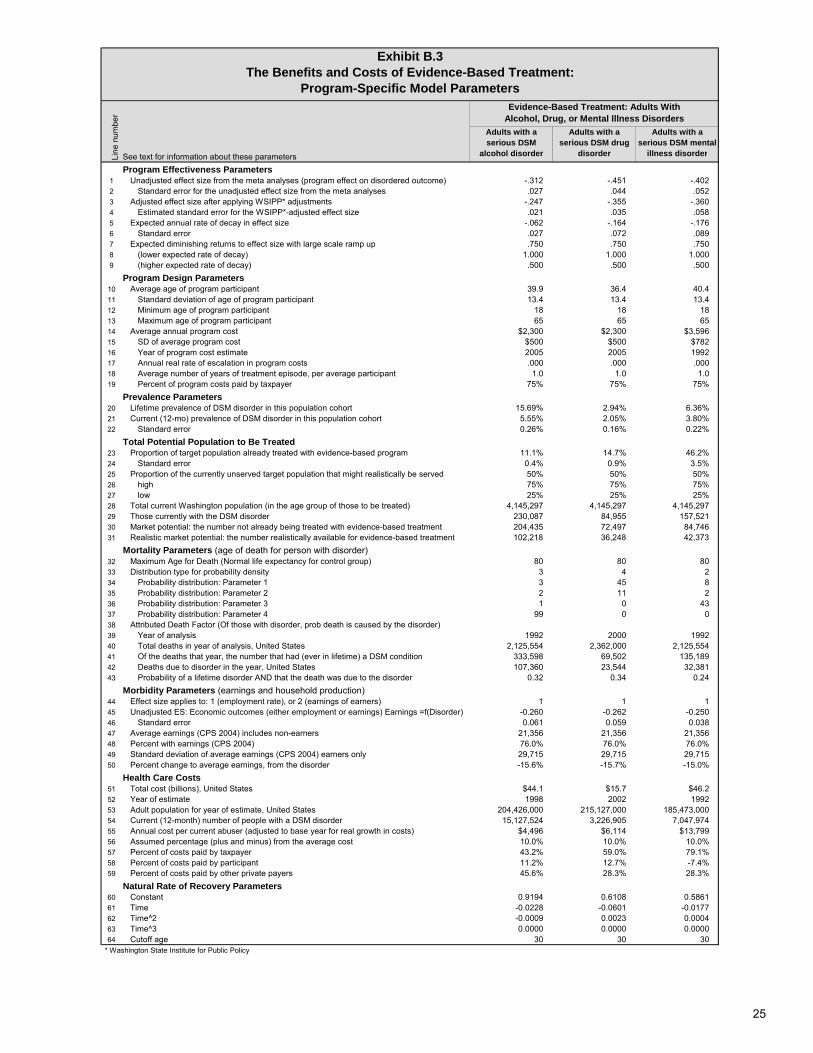
25

Adults with a serious DSM

alcohol disorder

Adults with a serious DSM drug

disorder

Adults with a serious DSM mental

illness disorder

Program Effectiveness Parameters1 Unadjusted effect size from the meta analyses (program effect on disordered outcome) -.312 -.451 -.4022 Standard error for the unadjusted effect size from the meta analyses .027 .044 .0523 Adjusted effect size after applying WSIPP* adjustments -.247 -.355 -.3604 Estimated standard error for the WSIPP*-adjusted effect size .021 .035 .0585 Expected annual rate of decay in effect size -.062 -.164 -.1766 Standard error .027 .072 .0897 Expected diminishing returns to effect size with large scale ramp up .750 .750 .7508 (lower expected rate of decay) 1.000 1.000 1.0009 (higher expected rate of decay) .500 .500 .500

Program Design Parameters10 Average age of program participant 39.9 36.4 40.411 Standard deviation of age of program participant 13.4 13.4 13.412 Minimum age of program participant 18 18 1813 Maximum age of program participant 65 65 6514 Average annual program cost $2,300 $2,300 $3,59615 SD of average program cost $500 $500 $78216 Year of program cost estimate 2005 2005 199217 Annual real rate of escalation in program costs .000 .000 .00018 Average number of years of treatment episode, per average participant 1.0 1.0 1.019 Percent of program costs paid by taxpayer 75% 75% 75%

Prevalence Parameters20 Lifetime prevalence of DSM disorder in this population cohort 15.69% 2.94% 6.36%21 Current (12-mo) prevalence of DSM disorder in this population cohort 5.55% 2.05% 3.80%22 Standard error 0.26% 0.16% 0.22%

Total Potential Population to Be Treated23 Proportion of target population already treated with evidence-based program 11.1% 14.7% 46.2%24 Standard error 0.4% 0.9% 3.5%25 Proportion of the currently unserved target population that might realistically be served 50% 50% 50%26 high 75% 75% 75%27 low 25% 25% 25%28 Total current Washington population (in the age group of those to be treated) 4,145,297 4,145,297 4,145,29729 Those currently with the DSM disorder 230,087 84,955 157,52130 Market potential: the number not already being treated with evidence-based treatment 204,435 72,497 84,74631 Realistic market potential: the number realistically available for evidence-based treatment 102,218 36,248 42,373

Mortality Parameters (age of death for person with disorder)32 Maximum Age for Death (Normal life expectancy for control group) 80 80 8033 Distribution type for probability density 3 4 234 Probability distribution: Parameter 1 3 45 835 Probability distribution: Parameter 2 2 11 236 Probability distribution: Parameter 3 1 0 4337 Probability distribution: Parameter 4 99 0 038 Attributed Death Factor (Of those with disorder, prob death is caused by the disorder)39 Year of analysis 1992 2000 199240 Total deaths in year of analysis, United States 2,125,554 2,362,000 2,125,55441 Of the deaths that year, the number that had (ever in lifetime) a DSM condition 333,598 69,502 135,18942 Deaths due to disorder in the year, United States 107,360 23,544 32,38143 Probability of a lifetime disorder AND that the death was due to the disorder 0.32 0.34 0.24

Morbidity Parameters (earnings and household production)44 Effect size applies to: 1 (employment rate), or 2 (earnings of earners) 1 1 145 Unadjusted ES: Economic outcomes (either employment or earnings) Earnings =f(Disorder) -0.260 -0.262 -0.25046 Standard error 0.061 0.059 0.03847 Average earnings (CPS 2004) includes non-earners 21,356 21,356 21,35648 Percent with earnings (CPS 2004) 76.0% 76.0% 76.0%49 Standard deviation of average earnings (CPS 2004) earners only 29,715 29,715 29,71550 Percent change to average earnings, from the disorder -15.6% -15.7% -15.0%

Health Care Costs51 Total cost (billions), United States $44.1 $15.7 $46.252 Year of estimate 1998 2002 199253 Adult population for year of estimate, United States 204,426,000 215,127,000 185,473,00054 Current (12-month) number of people with a DSM disorder 15,127,524 3,226,905 7,047,97455 Annual cost per current abuser (adjusted to base year for real growth in costs) $4,496 $6,114 $13,79956 Assumed percentage (plus and minus) from the average cost 10.0% 10.0% 10.0%57 Percent of costs paid by taxpayer 43.2% 59.0% 79.1%58 Percent of costs paid by participant 11.2% 12.7% -7.4%59 Percent of costs paid by other private payers 45.6% 28.3% 28.3%

Natural Rate of Recovery Parameters60 Constant 0.9194 0.6108 0.586161 Time -0.0228 -0.0601 -0.017762 Time^2 -0.0009 0.0023 0.000463 Time^3 0.0000 0.0000 0.000064 Cutoff age 30 30 30

* Washington State Institute for Public Policy

See text for information about these parameters

Evidence-Based Treatment: Adults With Alcohol, Drug, or Mental Illness Disorders

Line

num

ber


Program-Specific Model Parameters

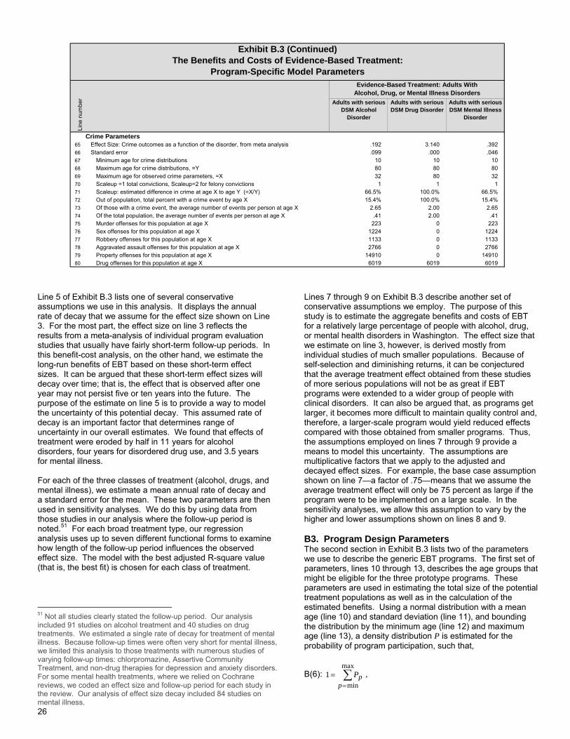
26

Adults with serious DSM Alcohol

Disorder

Adults with serious DSM Drug Disorder

Adults with serious DSM Mental Illness

Disorder

Crime Parameters65 Effect Size: Crime outcomes as a function of the disorder, from meta analysis .192 3.140 .39266 Standard error .099 .000 .04667 Minimum age for crime distributions 10 10 1068 Maximum age for crime distributions, =Y 80 80 8069 Maximum age for observed crime parameters, =X 32 80 3270 Scaleup =1 total convictions, Scaleup=2 for felony convictions 1 1 171 Scaleup: estimated difference in crime at age X to age Y (=X/Y) 66.5% 100.0% 66.5%72 Out of population, total percent with a crime event by age X 15.4% 100.0% 15.4%73 Of those with a crime event, the average number of events per person at age X 2.65 2.00 2.6574 Of the total population, the average number of events per person at age X .41 2.00 .4175 Murder offenses for this population at age X 223 0 22376 Sex offenses for this population at age X 1224 0 122477 Robbery offenses for this population at age X 1133 0 113378 Aggravated assault offenses for this population at age X 2766 0 276679 Property offenses for this population at age X 14910 0 1491080 Drug offenses for this population at age X 6019 6019 6019

Line

num

ber


Exhibit B.3 (Continued)The Benefits and Costs of Evidence-Based Treatment:

Program-Specific Model Parameters

Line 5 of Exhibit B.3 lists one of several conservative assumptions we use in this analysis. It displays the annual rate of decay that we assume for the effect size shown on Line 3. For the most part, the effect size on line 3 reflects the results from a meta-analysis of individual program evaluation studies that usually have fairly short-term follow-up periods. In this benefit-cost analysis, on the other hand, we estimate the long-run benefits of EBT based on these short-term effect sizes. It can be argued that these short-term effect sizes will decay over time; that is, the effect that is observed after one year may not persist five or ten years into the future. The purpose of the estimate on line 5 is to provide a way to model the uncertainty of this potential decay. This assumed rate of decay is an important factor that determines range of uncertainty in our overall estimates. We found that effects of treatment were eroded by half in 11 years for alcohol disorders, four years for disordered drug use, and 3.5 years for mental illness. For each of the three classes of treatment (alcohol, drugs, and mental illness), we estimate a mean annual rate of decay and a standard error for the mean. These two parameters are then used in sensitivity analyses. We do this by using data from those studies in our analysis where the follow-up period is noted.51 For each broad treatment type, our regression analysis uses up to seven different functional forms to examine how length of the follow-up period influences the observed effect size. The model with the best adjusted R-square value (that is, the best fit) is chosen for each class of treatment.

51 Not all studies clearly stated the follow-up period. Our analysis included 91 studies on alcohol treatment and 40 studies on drug treatments. We estimated a single rate of decay for treatment of mental illness. Because follow-up times were often very short for mental illness, we limited this analysis to those treatments with numerous studies of varying follow-up times: chlorpromazine, Assertive Community Treatment, and non-drug therapies for depression and anxiety disorders. For some mental health treatments, where we relied on Cochrane reviews, we coded an effect size and follow-up period for each study in the review. Our analysis of effect size decay included 84 studies on mental illness.

Lines 7 through 9 on Exhibit B.3 describe another set of conservative assumptions we employ. The purpose of this study is to estimate the aggregate benefits and costs of EBT for a relatively large percentage of people with alcohol, drug, or mental health disorders in Washington. The effect size that we estimate on line 3, however, is derived mostly from individual studies of much smaller populations. Because of self-selection and diminishing returns, it can be conjectured that the average treatment effect obtained from these studies of more serious populations will not be as great if EBT programs were extended to a wider group of people with clinical disorders. It can also be argued that, as programs get larger, it becomes more difficult to maintain quality control and, therefore, a larger-scale program would yield reduced effects compared with those obtained from smaller programs. Thus, the assumptions employed on lines 7 through 9 provide a means to model this uncertainty. The assumptions are multiplicative factors that we apply to the adjusted and decayed effect sizes. For example, the base case assumption shown on line 7—a factor of .75—means that we assume the average treatment effect will only be 75 percent as large if the program were to be implemented on a large scale. In the sensitivity analyses, we allow this assumption to vary by the higher and lower assumptions shown on lines 8 and 9. B3. Program Design Parameters The second section in Exhibit B.3 lists two of the parameters we use to describe the generic EBT programs. The first set of parameters, lines 10 through 13, describes the age groups that might be eligible for the three prototype programs. These parameters are used in estimating the total size of the potential treatment populations as well as in the calculation of the estimated benefits. Using a normal distribution with a mean age (line 10) and standard deviation (line 11), and bounding the distribution by the minimum age (line 12) and maximum age (line 13), a density distribution P is estimated for the probability of program participation, such that,

B(6): ∑=

=max

min1

ppP ,

27

where the distribution P is defined to be normally distributed with a mean age and its standard deviation. Lines 14 through 19 list the assumptions we made about the cost of EBT programs. These include estimates of the average cost per treatment episode, assumptions regarding the standard deviation for these average costs, and the extent to which EBT programs would be financed by tax dollars. Rather than costing-out each of the individual EBT programs examined, we assumed that EBT is the norm for those currently receiving services. Therefore, the observed average cost per treatment episode is a reasonable approximation of the average cost per episode of an average EBT program. Of course, to the extent the current practices do not represent evidence-based approaches, we may be under-estimating the cost of EBT programs. The average costs of EBT for alcohol, drug, and mental health are derived from two sources. According to one recent report, the average cost of EBT for alcohol or drug abuse in Washington State was $2,300 per episode in 2002.52 The report did not provide separate estimates for alcohol and drug treatment, therefore, the same figure is used for both program areas. A similar episode-based cost estimate for treatment of serious mental illness was not available for Washington State. Fortunately, the same study that we used to describe health care and other costs attributable to mental illness also provided an estimate of mental health treatment costs, which in 1992 dollars, averaged $3,596 per episode.53 Updated to current dollars, we assume this to be the cost of EBT for serious mental health disorders. B4. Prevalence Parameters To determine the size of the population in Washington that has a serious disorder that could be addressed with one of the three prototype EBT programs, we reviewed the national literature on the prevalence of the disorders in the general population. There have been several national studies conducted in the last 20 years to estimate the lifetime and current prevalence of serious alcohol, drug, and mental illness in the general population. Lines 20 to 22 show the estimates from our reading of the national literature. Line 20 shows the estimated lifetime probability of having one of the disorders. This parameter is used when we model the mortality effects of the disorders, described in Appendix B9. For alcohol and drug dependence, we use the lifetime prevalence rates listed in Harwood et al.54

The Harwood lifetime rates were taken from their analysis of the National Longitudinal Alcohol Epidemiologic Survey for adults ages 18 to 64. Harwood reports lifetime prevalence rates for males and females; we combine them into an overall average using 1992 census data on the ratio of males to females in the 18 to 64 age group. The estimate we used for a lifetime prevalence of serious mental illness, shown on line 20, was derived in the following manner. Harwood et al. (2000) provided an estimate of the 12-month prevalence of serious mental illness55 for males and females at .03 and .046, respectively, for an average rate of .038. This number accounts for comorbidity, that is, persons 52 T.M. Wickizer, A. Krupski, K. Stark, D. Mancuso, and K. Campbell. (in press). The Effect of Substance Abuse Treatment on Medicaid Expenditures among General Assistance Welfare Clients in Washington State. Milbank Quarterly. 53 Harwood et al., The economic costs of mental illness, page 3-6. 54 Harwood et al., The economic costs of alcohol and drug abuse. 55 Harwood et al., The economic costs of mental illness.

with more than one serious mental illness are counted only once. We estimated lifetime prevalence by summing lifetime prevalence rates reported for the National Comorbidity Survey Replication56 for schizophrenia, bipolar disorders, and serious forms of major depression and panic disorder. To account for comorbidity, we then multiplied by the ratio of Harwood’s 12-month prevalence to the sum of 12-month prevalences for each of these disorders. Note that this rate on line 20 is for severe diagnoses which the Harwood report defines to be schizophrenia, non-affective psychosis, manic depressive disorder, severe forms of major depression and panic disorder.57 In our study, we confine our economic analyses to these severe forms of mental disorders. Line 21 of Exhibit B.3 is the estimate we use in this study of the current (i.e. 12-month) prevalence of each disorder in the general population. For serious alcohol and drug disorders, we use the estimates provided in Narrow et al. (2002) which are based on their interpretation of the clinical significance of findings from the National Comorbidity Survey and the Epidemiologic Catchment Area study.58 For serious mental illness disorders, we use the estimate provided in Harwood et al.59 We account for the comorbidity between drug and alcohol dependency with the following calculations. Narrow et al. report a total disorder rate for any alcohol or drug disorder of 7.6 percent for the 18- to 54-year-old age group. They also report a 6.5 percent rate of alcohol disorders and a 2.4 percent rate for other drug use disorders. To account for comorbidity and avoid double counting people later in our analysis, we estimate the unique alcohol disorder rate as 5.5 percent (.055 = 0.076*(6.5/(6.5+2.4))) and the unique other drug disorder rate as 2.05 percent (.0205 = 0.076*(2.4/(6.5+2.4))). We estimate the size of the standard errors with the number of subjects in the National Comorbidity Survey (7,599). The associated standard errors are used in sensitivity analyses. B5. Total Potential Population to Be Treated We estimated two additional factors to help focus the analysis on the size of the population that could take advantage of the prototype EBT programs. First, we estimate the size of the disordered population already being treated with EBT programs in Washington. These estimates are shown on lines 23 and 24 of Exhibit B.3. For people with serious alcohol disorders and for those with serious illicit drug disorders, we analyzed the public use data set for the National Epidemiological Survey on Alcohol and Related Conditions (NESCAR). Among people indicating alcohol dependence in the past 12 months, we calculated the average percent and standard deviation that had been treated professionally for their alcohol disorder in the past 12 months. We used the same procedure for those with dependence on illicit drugs. For people with serious mental illness disorders, we relied on estimates of treatment rates by Kessler et al. based on the National Comorbidity Survey.60 On lines 25 to 27 we also make additional restrictions on the size of the population that might be treated with EBT programs. It is never possible to completely saturate a market, so we provide factors to estimate low, medium, and 56 R. Kessler et al. Prevalence, severity, and comorbidity of 12-month DSM-IV disorders in the National Comorbidity Survey Replication. 57 Harwood et al., The economic costs of mental illness. Table 4.7. 58 Narrow et al., Revised prevalence estimates of mental disorders. 59 Harwood et al., The economic costs of mental illness. Table 4.7. 60 R. Kessler, P. Berglund, M. Bruce, J. Koch, E. Laska, P. Leaf, R. Mandersheid, R. Rosenheck, E. Walters, and P. Wang. (2001). The prevalence and correlates of untreated serious mental illness. Health Services Research, 36(6): 987-1007.

28

high market penetration rates. These alternative rates are used in the sensitivity analysis described in Appendix B12. The factors described above are used to compute the total size of the current population in Washington that: (a) has a serious disorder, (b) is not currently being treated, and (c) might be realistically treated with a prototype EBT. Line 28 of Exhibit B.3 reports the size of the total population in Washington between the minimum and maximum age groups described on lines 12 and 13. The Washington population estimate is taken from the Washington State Office of Financial Management, and the actual population estimates are shown in Exhibit B.2.61 To this figure, we then applied the 12-month prevalence estimate (from line 21) to produce line 29: the estimated total current number of people in Washington with the disorder. Line 30 then subtracts the estimated percentage of the population already being treated with EBT programs (from line 23). Finally, line 31 applied the base assumption about the realistic potential (from line 25) to enroll disordered people in a prototype EBT. B6. Morbidity Parameters and Methods Prior studies of the costs of alcohol, drug, and mental illness disorders have found that, among people with the disorders, performance in the economic marketplace is reduced.62 To provide an independent test of this hypothesis, we conducted several meta-analyses. We sought to determine if existing research studies indicate that either an individual’s level of earnings conditional on employment, or the rate of employment alone, was significantly related to the presence of having an alcohol, drug, or mental illness disorder. We reviewed the literature on the topics and used the meta-analytic methods described in Appendix A to this report. Exhibit B.4 summarizes the results of our meta-analyses. We found that all three disorders are significantly related to the probability of employment, but not earnings conditional on employment. The effect sizes for employment from the meta-analyses are shown on line 45 of Exhibit B.3 and the associated standard errors are listed on line 46. To find the marginal effect of a disorder on average earnings levels (via the effect on employment rates), we compute the following:

B(7): AE

AEESERERAE

EEt

⎟⎠

⎞⎜⎝

⎛ −+=

2)^2

)(arcsinsin(*,

where EE is the estimated earnings effect for each of the evidence-based treatments, t, and represents the percentage change in average earnings; AE is the average earnings of earners and non-earners taken as a whole (this estimate, shown on line 47, comes from the CPS; ER is the employment rate (shown on line 48 of Exhibit B.3, also from the CPS) and ES is the effect size of the effect of having a disorder on ER (shown on line 45, from the meta-analysis). Since the arcsine transformation is used to compute the effect size in the meta-analyses, as described in Appendix A, that effect is reversed here to return the unit change.

61 Washington State Office of Financial Management, http://www.ofm.wa.gov/pop/default.asp 62 See: (a) Harwood, Updating estimates of the economic costs of alcohol abuse in the United States, from Table 3; (b) Office of National Drug Control Policy. The economic costs of drug abuse in the United States, from Table III-1; and (c) Harwood et al., The economic costs of mental illness, from Table 6.1.

To compute the earnings effect of an incidence of a DSM disorder, we begin with the following equation: B(8): INFLATIONFRINGEEARNINGSE aa **= For each age a, the total earnings of a person Ea is the annual EARNINGS taken from the Current Population Survey for that age, shown on Exhibit B.2, times the FRINGE benefit multiple, shown on line 3 of Exhibit B.1, times the INFLATION adjustment from Exhibit B.2 to inflate the CPS series (denominated in 2004 dollars) to the year chosen for this analysis (2006 dollars). The annual cash flows of lost earnings associated with having a disorder of type t is estimated with this process:

B(9): 1***)1(*$ 11 −+= −−+∑ tpt

yP

pypty PPEEEREE

In this equation, $Ety is the annual cash flow of lost earnings for a person with disorder type t in year y, where y is the number of years following participation in an EBT. The subscript y equals 1 during the year that a person is administered an EBT.

29

Homogeneity Test

ES p-value p-value ES p-valueEmployment =f(alcohol disorder) 11 -.183 0.000 0.000 -.239 0.000

Wages =f(alcohol disorder) 5 .004 0.701 0.124 na na

Employment =f(DSM mental illness) 8 -.246 0.000 0.000 -.250 0.000

Wages =f(DSM mental illness) 7 -.140 0.000 0.000 -.213 0.000

Employment =f(drug disorder) 6 -.230 0.000 0.000 -.262 0.000

Wages =f(drug disorder) 1 .000 0.981 na na na

Crime =f(Mental Illness) 3 .337 0.000 0.001 .392 0.000

Crime =f(Alcohol Disorder) 3 .176 0.000 0.000 .192 0.053

Zuvekas, Cooper, & Buchmueller, 2005 Employment =f(alcohol disorder)Mullahy and Sindelar, 1993 Employment =f(alcohol disorder)Mullahy and Sindelar, 1996 Employment =f(alcohol disorder)Mullahy and Sindelar, 1997 Employment =f(alcohol disorder)Terza, 2002 Employment =f(alcohol disorder)Terza, (undated) Employment =f(alcohol disorder)Chevrou-Severac and Jeanrenaud, 2002 Employment =f(alcohol disorder)Feng et al., 2001 Employment =f(alcohol disorder)Auld, 2002 Employment =f(alcohol disorder)MacDonald & Shields, 2004 Employment =f(alcohol disorder)Cook & Peters, 2005 Employment =f(alcohol disorder)Zuvekas, Cooper, & Buchmueller, 2005 Wages of workers =f(alcohol disorder)Mullahy and Sindelar, 1993 Wages of workers =f(alcohol disorder)Zarkin et al., 1998 Wages of workers =f(alcohol disorder)Kenkel and Ribar, 1994 Wages of workers =f(alcohol disorder)Bray, (2005) Wages of workers =f(alcohol disorder)Harwood et al., 2000 Employment =f(DSM mental illness disorder)Ettner et al., 1997 Employment =f(DSM mental illness disorder)Farahati et al., 2003 Employment =f(DSM mental illness disorder)Savoca, 2000 Employment =f(DSM mental illness disorder)Alexandre & French, 2001 Employment =f(DSM mental illness disorder)Kessler et al., 1999 Employment =f(DSM mental illness disorder)Hamilton et al., 1997 Employment =f(DSM mental illness disorder)Chatterji et al., 2005 Employment =f(DSM mental illness disorder)Ettner et al., 1997 Wages of workers =f(DSM mental illness disorder)Marcotte, 2003 Wages of workers =f(DSM mental illness disorder)Kessler & Frank, 1997 Wages of workers =f(DSM mental illness disorder)Frank & Gertler, 1991 Wages of workers =f(DSM mental illness disorder)Bartel & Taubman, 1986 Wages of workers =f(DSM mental illness disorder)French & Zarkin, 1998 Wages of workers =f(DSM mental illness disorder)Stewart et al., 2003 Wages of workers =f(DSM mental illness disorder)DeSimone, 2002 Employment =f(drug disorder)Buchmueller and Zuvekas, 1998 Employment =f(drug disorder)Zuvekas, Cooper, & Buchmueller, 2005 Employment =f(drug disorder)Terza, (undated) Employment =f(drug disorder)Alexandre & French, 2004 Employment =f(drug disorder)French, Roebuck, Alexandre, 2001 Employment =f(drug disorder)Zuvekas, Cooper, & Buchmueller, 2005 Wages of workers =f(drug disorder)Hodgins et al., 1996 crime =f(mental illness)Tiihonen, 1997 crime =f(mental illness)Wallace et al., 2004 crime =f(mental illness)Carpenter, 2003 crime =f(alcohol disorder)Fergusson and Horwood, 2000 crime =f(alcohol disorder)Lipsey et al., 1996 crime =f(alcohol disorder)

Weighted Mean Effect Size & p-value

Number of Effect

Sizes Included

in the Analysis


Fixed EffectsModel


Exhibit B.4Meta-Analytic Estimates of Standardized Mean Difference Effect Sizes

Weighted Mean Effect Size & p-value

Used to estimateStudies (complete citation on next page)

30

Exhibit B.4a Citations to Studies in Exhibit B.4

Alexandre, P. & French, T. (2001). Labor supply of poor residents in metropolitan Miami, Florida: The role of depression and the co-morbid effects of substance use. The Journal of Mental Health Policy and Economics, 4(4): 161-173.

Alexandre, P.K. & French, M.T. (2004). Further evidence on the labor market effects of addiction: Chronic drug use and labor supply in metropolitan Miami. Contemporary Economic Policy, 22(3): 382-393.

Auld, M.C. (2002). Robust system estimation of causal effects on binary outcomes, with application to effect of alcohol abuse on employment. Calgary, Alberta, Canada: Department of Economics, University of Calgary. http://econ.ucalgary.ca/research/200301WP.pdf.

Bartel, A. & Taubman, P. (1986). Some economic and demographic consequences of mental illness. Journal of Labor Economics, 4(2): 243-256. Bray, J. W. (2005). Alcohol use, human capital, and wages. Journal of Labor Economics, 23(2): 279-312. Buchmueller, T.C. & Zuvekas, S.H. (1998). Drug use, drug abuse, and labour market outcomes. Health Economics, 7(3): 229-45. Carpenter, C. (2003). Does heavy alcohol use cause crime? Evidence from underage drunk driving laws. Unpublished paper. Chatterji, P., Alegría, M., Lu, M., & Takeuchi, D. (2005). Psychiatric disorders and labor market outcomes: Evidence from the National Latino and Asian American Study

(Working Paper No. 11893). Washington, DC: National Bureau of Economic Research. Chevrou-Severac, H. & Jeanrenaud, C. (2002). The impact of alcohol abuse on employment in Switzerland. Neuchatel, Switzerland: IRER.

http://perso.wanadoo.fr/ces/Pages/english/Poster17.pdf. Cook, P.J. & Peters, B.L. (2005). The myth of the drinker's bonus (Working Paper No. W11902). Washington, DC: National Bureau of Economic Research. DeSimone, J. (2002). Illegal drug use and employment. Journal of Labor Economics, 20(4): 952-977. Ettner, S.L., Frank, R.G., & Kessler, R.C. (1997). The impact of psychiatric disorders on labor market outcomes. Industrial & Labor Relations Review, 51(1): 64-81. Farahati, F., Booth, B., & Wilcox-Gők, V. (2003). Employment effects of comorbid depression and substance use. DeKalb, IL: Northern Illinois University, Department of

Economics. Feng, W., Zhou, W., Butler, J., Booth, B., & French, M. (2001). The impact of problem drinking on employment. Health Economics, 10(6): 509-521. Fergusson, D.M. & Horwood, L.J. (2000). Alcohol abuse and crime: A fixed-effects regression analysis. Addiction, 95(10): 1525-1536. Frank, R. & Gertler, P. (1991). An assessment measurement error bias for estimating the effect of mental distress on income. The Journal of Human Resources, 26(1): 154-

164. French, M.T. & Zarkin, G.A. (1998). Mental health, absenteeism and earnings at a large manufacturing worksite. The Journal of Mental Health Policy and Economics, 1(4):

161-172. French, M.T., Roebuck, M.C., and Alexandre, P.K. (2001). Illicit drug use, employment, and labor force participation. Southern Economic Journal, 68(2): 349-368. Hamilton, V.H., Merrigan, P., & Dufresne, E. (1997). Down and out: estimating the relationship between mental health and unemployment. Health Economics, 6(4): 397-406. Harwood, H. (2000). The economic cost of mental illness, 1992. Fairfax, VA: The Lewin Group. Hodgins, S., Mednick, S.A., Brennan, P.A., Schulsinger, F., & Engberg, M. (1996). Mental disorder and crime. Evidence from a Danish birth cohort. Archives of General

Psychiatry, 53(6): 489-96. Kenkel, D.S. & Ribar, D.C. (1994). Alcohol consumption and young adults' socioeconomic status. Brookings papers on economic activity: Microeconomics: 119-161. Kessler, R.C. & Frank, R. (1997). The impact of psychiatric disorders on work loss days. Psychological Medicine, 27(4): 861-873. Kessler, R.C., Barber, C., Birnbaum, H.G., Frank, R.G., Greenberg, P.E., Rose, R.M., et al. (1999). Depression in the workplace: Effects on short-term disability. Health

Affairs, 18(5): 163-171. Lipsey, M.W., Wilson, D.B., Cohen, M.A., & Derzon, J.H. (1996). Is there a causal relationship between alcohol use and violence? A synthesis of evidence. In M. Galanter

(Ed.), Recent Developments in Alcoholism, Volume 13: Alcoholism and Violence (pp. 245-282). New York: Plenum Press. MacDonald, Z. & Shields, M. (2004). Does problem drinking affect employment? Evidence from England. Health Economics, 13 (2): 139-155. Marcotte, D.E. & Wilcox-Gők, V. (2003). Estimating earnings losses due to mental illness: A quantile regression approach. The Journal of Mental Health Policy and

Economics, 6(3): 123-134. Mullahy, J. & Sindelar, J.L. (1993) Gender differences in labor market effects of alcoholism. The American Economic Review, 81(2): 161-165. Mullahy, J. & Sindelar, J.L. (1996). Employment, unemployment, and problem drinking. Journal of Health Economics, 15(4): 409-34. Mullahy, J. & Sindelar, J.L. (1997). Women and work: Tipplers and teetotalers. Health Economics, 6(5): 533-537. Savoca, E. & Rosenheck, R. (2000). The civilian labor market experiences of Vietnam-era veterans: The influence of psychiatric disorders. The Journal of Mental Health

Policy and Economics, 3(4): 199-207. Stewart, W.F., Ricci, J.A., Chee, E., Hahn, S.R., & Morganstein, D. (2003). Cost of lost productive work time among US workers with depression. Journal of the American

Medical Association, 289(23): 3135- 3144. Terza, J.V. (2002). Alcohol abuse and employment: A second look. Journal of Applied Econometrics, 17(4): 393-404. Terza, J.V. (n.d.). Assessing the impact of substance abuse on employment status. Charleston, SC: Medical University of South Carolina, Department of Health

Administration and Policy, Center for Health Economic and Policy Studies. http://people.musc.edu/~terza/empfina2.pdf. Tiihonen, J., Isohanni, M., Räsänen, P., Koiranen, M., & Moring, J. (1997). Specific major mental disorders and criminality: A 26-year prospective study of the 1966 northern

Finland birth cohort. American Journal Psychiatry, 154(6): 840-845. Wallace, C., Mullen, P.E., & Burgess, P. (2004). Criminal offending in schizophrenia over a 25-year period marked by deinstitutionalization and increasing prevalence of

comorbid substance use disorder. American Journal of Psychiatry, 161(4): 716-727. Zarkin, G.A., French, M.T., Mroz, T., & Bray, J.W. (1998). Alcohol use and wages: New results from the National Household Survey on Drug Abuse. Journal of Health

Economics, 17(1): 53-68. Zuvekas, S., Cooper, P.F., Buchmueller, T.C. (2005). Health behaviors and labor market status: The impact of substance abuse (Working Paper No. 05013). Rockville, MD:

US Department of Health and Human Services, Agency for Healthcare Research and Quality. http://gold.ahrq.gov.

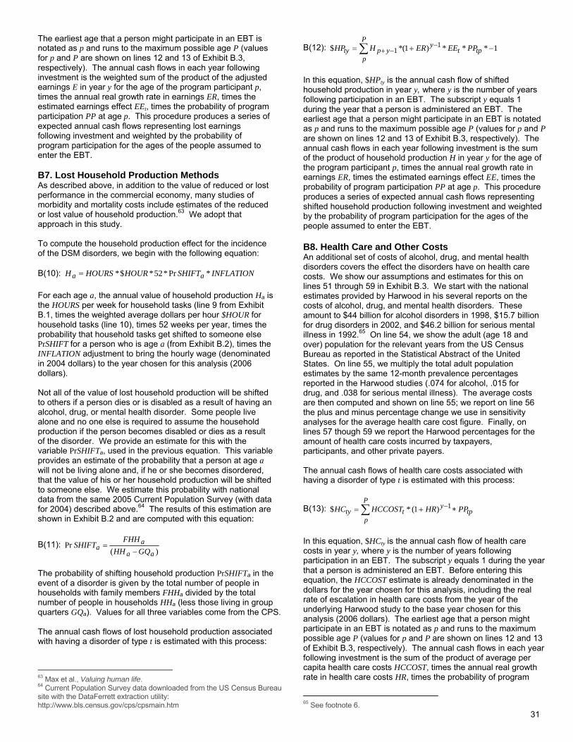
31

The earliest age that a person might participate in an EBT is notated as p and runs to the maximum possible age P (values for p and P are shown on lines 12 and 13 of Exhibit B.3, respectively). The annual cash flows in each year following investment is the weighted sum of the product of the adjusted earnings E in year y for the age of the program participant p, times the annual real growth rate in earnings ER, times the estimated earnings effect EEt, times the probability of program participation PP at age p. This procedure produces a series of expected annual cash flows representing lost earnings following investment and weighted by the probability of program participation for the ages of the people assumed to enter the EBT. B7. Lost Household Production Methods As described above, in addition to the value of reduced or lost performance in the commercial economy, many studies of morbidity and mortality costs include estimates of the reduced or lost value of household production.63 We adopt that approach in this study. To compute the household production effect for the incidence of the DSM disorders, we begin with the following equation: B(10): INFLATIONSHIFTHOURHOURSH aa *Pr*52*$*= For each age a, the annual value of household production Ha is the HOURS per week for household tasks (line 9 from Exhibit B.1, times the weighted average dollars per hour $HOUR for household tasks (line 10), times 52 weeks per year, times the probability that household tasks get shifted to someone else PrSHIFT for a person who is age a (from Exhibit B.2), times the INFLATION adjustment to bring the hourly wage (denominated in 2004 dollars) to the year chosen for this analysis (2006 dollars). Not all of the value of lost household production will be shifted to others if a person dies or is disabled as a result of having an alcohol, drug, or mental health disorder. Some people live alone and no one else is required to assume the household production if the person becomes disabled or dies as a result of the disorder. We provide an estimate for this with the variable PrSHIFTa, used in the previous equation. This variable provides an estimate of the probability that a person at age a will not be living alone and, if he or she becomes disordered, that the value of his or her household production will be shifted to someone else. We estimate this probability with national data from the same 2005 Current Population Survey (with data for 2004) described above.64 The results of this estimation are shown in Exhibit B.2 and are computed with this equation:

B(11): )(

Praa

aa GQHH

FHHSHIFT

−=

The probability of shifting household production PrSHIFTa in the event of a disorder is given by the total number of people in households with family members FHHa divided by the total number of people in households HHa (less those living in group quarters GQa). Values for all three variables come from the CPS. The annual cash flows of lost household production associated with having a disorder of type t is estimated with this process:

63 Max et al., Valuing human life. 64 Current Population Survey data downloaded from the US Census Bureau site with the DataFerrett extraction utility: http://www.bls.census.gov/cps/cpsmain.htm

B(12): 1***)1(*$ 11 −+= −−+∑ tpt

yP

pypty PPEEERHHP

In this equation, $HPty is the annual cash flow of shifted household production in year y, where y is the number of years following participation in an EBT. The subscript y equals 1 during the year that a person is administered an EBT. The earliest age that a person might participate in an EBT is notated as p and runs to the maximum possible age P (values for p and P are shown on lines 12 and 13 of Exhibit B.3, respectively). The annual cash flows in each year following investment is the sum of the product of household production H in year y for the age of the program participant p, times the annual real growth rate in earnings ER, times the estimated earnings effect EE, times the probability of program participation PP at age p. This procedure produces a series of expected annual cash flows representing shifted household production following investment and weighted by the probability of program participation for the ages of the people assumed to enter the EBT. B8. Health Care and Other Costs An additional set of costs of alcohol, drug, and mental health disorders covers the effect the disorders have on health care costs. We show our assumptions and estimates for this on lines 51 through 59 in Exhibit B.3. We start with the national estimates provided by Harwood in his several reports on the costs of alcohol, drug, and mental health disorders. These amount to $44 billion for alcohol disorders in 1998, $15.7 billion for drug disorders in 2002, and $46.2 billion for serious mental illness in 1992.65 On line 54, we show the adult (age 18 and over) population for the relevant years from the US Census Bureau as reported in the Statistical Abstract of the United States. On line 55, we multiply the total adult population estimates by the same 12-month prevalence percentages reported in the Harwood studies (.074 for alcohol, .015 for drug, and .038 for serious mental illness). The average costs are then computed and shown on line 55; we report on line 56 the plus and minus percentage change we use in sensitivity analyses for the average health care cost figure. Finally, on lines 57 though 59 we report the Harwood percentages for the amount of health care costs incurred by taxpayers, participants, and other private payers. The annual cash flows of health care costs associated with having a disorder of type t is estimated with this process:

B(13): tpy

P

ptty PPHRHCCOSTHC ∗+= −∑ 1)1(*$

In this equation, $HCty is the annual cash flow of health care costs in year y, where y is the number of years following participation in an EBT. The subscript y equals 1 during the year that a person is administered an EBT. Before entering this equation, the HCCOST estimate is already denominated in the dollars for the year chosen for this analysis, including the real rate of escalation in health care costs from the year of the underlying Harwood study to the base year chosen for this analysis (2006 dollars). The earliest age that a person might participate in an EBT is notated as p and runs to the maximum possible age P (values for p and P are shown on lines 12 and 13 of Exhibit B.3, respectively). The annual cash flows in each year following investment is the sum of the product of average per capita health care costs HCCOST, times the annual real growth rate in health care costs HR, times the probability of program

65 See footnote 6.

32

participation PP at age p. This procedure produces a series of expected annual cash flows representing health care costs following investment and weighted by the probability of program participation for the ages of people assumed to enter the EBT. B9. Mortality Parameters and Methods If the prevalence of alcohol, drug, or mental health disorders is reduced with EBT, then one form of benefits will be that people live longer and, as a result, are more productive in the marketplace. All cost-of-illness studies estimate these mortality-related effects. The mortality methods we employed in this study required three pieces of information. The first is shown on line 32 on Exhibit B.3: the normal life expectancy for the average adult today. We estimated this parameter from the Center for Disease Control for the average life expectancy of a 40-year-old, which corresponds roughly to the average age of a person in our prototype programs.66 For people who die of a disorder, we estimated the probability of death by age of death. We used data from the Washington State Vital Statistics dataset. For alcohol and drug related deaths, we counted the age of all deaths in Washington with ICD-10 death codes where a certain percentage of the deaths had been attributed to the disorder. For alcohol related deaths, we used the attribution factors for the individual diagnoses contained in Max et al.67 For drug related deaths, we used the attribution factors contained in Harwood et al.68 For suicide deaths, we used all deaths in Washington coded as a suicide. Using these counts of actual Washington deaths, we then estimated a probability density distribution for each disorder (alcohol, drug, and suicide). Lines 33 through 37 contain the parameters of these equations. We found that for alcohol related deaths, a Beta distribution best fit the actual Washington data; for drug related deaths, a Normal distribution fit the data; and for suicides (mental health deaths), a Weibull distribution was best. For alcohol and drug deaths, we estimated the distributions with Washington data for 2004; for suicides we used Washington data for 2003 and 2004 to increase the sample size. For each disorder, this process produces: B(14): aDD , where DDa is the probability density distribution of a person with an alcohol or drug disorder or a suicide at age a, and the distributions are defined by a Beta, Normal, or Weibull, respectively. Not everyone who has an alcohol, drug, or mental illness disorder dies of the disorder. Lines 38 through 43 of Exhibit B.3 list the parameters we used to estimate the probability that a person with a history of a disorder dies of the disorder. For the United States, Harwood estimated the total number of deaths in 1992 (for alcohol), 2000 (for drugs), and 1992 (for suicides) that were caused by having an alcohol, drug, or mental disorder, respectively. These values are shown on line 42, while line 40 shows the total number of deaths in the United States (for people 15 or older) during those years. Line 41 is the product of line 40

66 D. Hoyert, H. Kung, and B. Smith. (2005). Expectation of life by age, race, and sex: United States, final 2002 and preliminary 2003. US Department of Health and Human Services, Centers for Disease Control and Prevention, National Vital Statistics Report, 53(15), Table 6. http://www.cdc.gov/nchs/data/nvsr/nvsr53/nvsr53_15.pdf 67 Max et al., Valuing human life, Table 2. 68 Office of National Drug Control Policy. (2004).The economic costs of drug abuse in the United States, Table B-10. http://www.whitehousedrugpolicy. gov/publications/economic_costs/economic_costs.pdf

and line 20, the lifetime prevalence of each disorder. This provides an estimate of the number of people who died in the relevant year who had a disorder sometime in their lives. Line 43 is computed as line 42 divided by line 41; it is the attributed death factor, ADF, for each disorder. The annual cash flows of lost earnings and household production associated with having a death caused by having a disorder of type t is estimated with this process: B(15):

K∑ −+−

−+−+ ++=P

pytp

rypypty DDERHED 1

111 *)1(*][$

tpt PADF **L In this equation, $Dty is the cash flow of lost earnings E and household production H in year y, where y is the number of years following participation in an EBT. The subscript y equals 1 in the year that a person is administered an EBT, and runs to M—the maximum follow-up period for estimating cash flows. The earliest age that a person might participate in an EBT is notated as p and runs to the maximum possible age P (values for p and P are shown on lines 12 and 13 of Exhibit B.3, respectively). The annual cash flows in each year following investment is computed as the weighted sum of the product of the adjusted earnings E by year y for the age of the program participant p, plus the household production H by year y for the age of the program participant p, times the real growth rate in earnings ER, times the probability of a death occurring, DD, by year y for the age of the program participant, times the attributed death factor ADF for the disorder, times the probability of program participation PP for a participant of age p. This procedure produces a series of expected annual cash flows representing lost earnings and lost household production following investment and weighted by the probability death and of program participation for the ages of the people assumed to enter the EBT. B10. Crime Parameters The effect that alcohol, drug, and mental health disorders have on crime is estimated in a two-step process. First, we use meta-analyses to examine the existing research literature on the linkage between each of these disorders and crime. Second, if the meta-analyses reveal a statistically significant relationship, we then use the Institute’s cost-of-crime model to estimate the effects that the increased levels of crime have on taxpayers (who fund the criminal justice system) and crime victims (who suffer out-of-pocket costs and pain and suffering costs when they are victimized). Then, to the degree that an evidence-based treatment reduces the incidence of a disorder, the estimated costs of crime are also reduced via this linkage. In Exhibit B.4 we list the results of the meta-analyses we performed on the linkage between the disorders and crime. We only found a few studies where the research design was robust. These few studies did provide some evidence of a statistically significant relationship between alcohol disorder and crime, and between mental illness and crime. We were unable to locate studies establishing a relationship between drug disorders and crime; this is a result consistent with other inquires into this topic.69 Nonetheless, in Washington State the consumption of these substances is illegal and, therefore,

69 See, for example: H. White, & D. Gorman. (2000). Dynamics of the drug crime relationship. In G. Lafree (Ed.), Criminal Justice 2000: Volume 1: The nature of crime: continuity and change (NCJ 182408, pp. 151-218). Washington, DC: US Department of Justice, Office of Justice Programs, National Institute of Justice. http://www.ncjrs.org/criminal_justice2000/vol_1/02d.pdf.

33

these drug crimes can result in a criminal justice system response including arrest, prosecution, and a full range of sentencing outcomes. These effects are modeled. The Institute’s model of the costs of crime has been described in detail elsewhere; the interested reader can find a full description of the routines used to calculate costs in the earlier reports.70 B11. Marginal Treatment Effect The estimated benefits of treatment are determined by the marginal effectiveness, over time, of EBT. The following equation is used to estimate the marginal treatment effect MTE for a person in an EBT treating a disorder of type t:

B(16): 2)^2

)()(arcsinsin( ty

tytytyES

NNMTE +−= ,

where B(17): t

yttty scaleupdecayrateESES ∗+∗= −1)1( ,

and where B(18): 32 *3*2*1 yNRtbyNRtbyNRtbNRtaNty +++= . For each of the three prototype programs t, we estimate the marginal treatment effect with the parameters in these equations. The variable Nty is the “natural rate of recovery” from a disorder without treatment in year y for treatment type t, where y is a year following participation in an EBT. The subscript y equals 1 during the year that a person is administered an EBT. We estimated years from onset to “natural recovery” using data from the 2001–2002 National Epidemiologic Survey on Alcohol and Related Conditions (NESARC).71 The NESARC is a longitudinal survey conducted by the federal National Institute on Alcohol Abuse and Alcoholism. The 2001–2002 NESARC is the first wave of the survey, with a sample of 43,093 respondents representative of the US adult population 18 years of age and older. We performed separate analyses for respondents who reported ever having the following conditions: alcohol dependence, substance dependence, major depression, dysthymia, mania or hypomania, panic disorders and agoraphobia (anxiety), social phobia, specific phobia, and generalized anxiety. We analyzed the NESARC data using the generalized least-squares estimation method that modeled the elapse (in years) between the onset of a condition and the year in which the last episode of symptoms was reported. To simulate “natural recovery,”72 we estimated the elapsed time only for respondents who reported no treatment since onset. Each estimation model includes the following covariates: age at the interview, age at the onset of the condition, sex, and high school diploma status. In addition, the model on alcohol dependence includes the covariates of ever having substance dependence and ever having a DSM-IV diagnosis of mental illness; the model on substance dependence includes the covariates of ever having alcohol dependence and also ever having a DSM-IV diagnosis of mental illness; and the models for mental illness conditions each include the covariates of ever having alcohol dependence

70 See footnote 5. 71 http://niaaa.census.gov/ 72 The term “recovery” refers to situations in which the last episode of symptoms had occurred no later than a year prior to the interview. It should be noted that this term is not used in the strict meaning as “cured” because in some situations the absence of symptoms before the interview could just be the “breathing” period between episodes.

and substance dependence. The analyses were performed using the SAS procedure of SURVEYREG. SURVEYREG is specially designed for regression analyses involving sample survey data. The procedure allows for adjustments for complex sample designs, including sample stratification, clustering, and unequal weights.73 The parameters shown on lines 60 through 63 in Exhibit B.3 are the parameters for a third degree polynomial for each prototype; for use in the simulation model, these are linear representations of the logistic models estimated with SAS. The determination of the effect size that is used for each year, ESty is computed with the short-run effect size, ESt, for each prototype evidence-based treatment, discussed elsewhere in this Appendix. These effect sizes were almost always obtained from studies with quite short follow-up periods, usually around a year. To account for the possibility that these short-run effect sizes might decay over the long run, we estimated decay rates, decayratet, for each prototype treatment. We describe how we obtained estimates for the decay rate in Appendix B2. In addition, also as described in Appendix B2, we multiplied the effect sizes by a factor, scaleupt, that is designed to reflect reduction in effect sizes that are likely to occur when small-scale programs are expanded significantly. B12. Sensitivity Analysis The model as described in this Appendix produces a unique result given the set of inputs listed. As we describe, however, there is a significant amount of uncertainty around many of the inputs. For most inputs to the model, we determine the range of uncertainty with the standard errors or standard deviations from relevant statistics of the underlying data for each parameter. For a few other parameters, we hypothesized low and high ranges to place bounds on our estimates of uncertainty. After we specified ranges of uncertainty on each of the inputs, we then used a simulation approach to determine how sensitive the final result is to these levels of uncertainty. To conduct the simulation, we used Palisade Corporation’s @RISK® simulation software. Using a Monte Carlo approach to the simulation, the software randomly draws from the user-designated input variables after a particular type of probability distribution and its parameters have been specified for the input. We ran a Monte Carlo simulation for 10,000 cases. Exhibit B.5 shows input variables along with the specified probability distributions that we used in the simulation.

73 SAS Institute Inc. 2004. SAS OnlineDoc® 9.1.2. Cary, NC: SAS Institute Inc.

34

Adults with a serious DSM

alcohol disorder

Adults with a serious DSM drug

disorder

Adults with a serious DSM mental

illness disorder

1. Program Effectiveness ParametersAdjusted effect size after applying WSIPP* adjustments Normal -.247 -.355 -.360

Estimated standard error for the WSIPP-adjusted effect size .021 .035 .058Expected annual rate of decay in effect size Normal -.062 -.164 -.176

Standard error .027 .072 .089Expected diminishing returns to effect size with large scale ramp up Triangular .750 .750 .750

(lower expected rate of decay) 1.000 1.000 1.000(higher expected rate of decay) .500 .500 .500

2. Program Design ParametersAverage annual program cost Normal $2,300 $2,300 $3,596

Standard deviation of average program cost $500 $500 $7823. Prevalence Parameters

Current (12-mo) prevalence of DSM disorder in this population cohort Normal 5.55% 2.05% 3.80%Standard error 0.26% 0.16% 0.22%

4. Potential Population to be TreatedProportion of target population already treated with evidence-based program Normal 11.1% 14.7% 46.2%

Standard error 0.4% 0.9% 3.5%Proportion of the currently unserved target population that might realistically be served Triangular 50% 50% 50%

high 75% 75% 75%low 25% 25% 25%

5. Morbidity Parameters (earnings and household production)Employment outcomes =f(Disorder) Normal -0.260 -0.262 -0.250

Standard error 0.061 0.059 0.0386. Health Care Costs

Annual cost/ current abuser (adjusted to base year for real growth in costs) Triangular $4,496 $6,114 $13,799Assumed percentage (plus and minus) from the average cost 10.0% 10.0% 10.0%

7. General Model Parameters High Medium LowDiscount Rate Discrete (equal %) .070 .050 .030Real annual rate of growth in earnings Triangular .023 .013 .003Real annual rate of growth in health care costs Triangular .044 .034 .024

* Washington State Institute for Public Policy


See text for information about these parameters

Probability Distribution Type in @RISK ®


Model Parameters Varied in the Monte Carlo Simulations

For further information, contact Steve Aos at (360) 586-2740; [email protected]

Document No. 06-06-3901

Washington State Institute for Public Policy

The Washington State Legislature created the Washington State Institute for Public Policy in 1983. A Board of Directors—representing the legislature, the governor, and public universities—governs the Institute and guides the development of all activities. The Institute’s mission is to carry out practical research, at legislative direction, on issues of importance to Washington State.

evidence-based treatment of alcohol, drug, and mental health disorders

Documents