News IData foRanganUniversiChristoUniversiStephanUniversiMark EUniversiWorkingApril 20 _______DepartmUnivers0002, PrSouth ATel: +27

Implied Vor the USAn Gupta ity of Pretor

os Kollias ity of Thessanos Papadity of Thessa

E. Wohar ity of Nebrag Paper: 201017

__________ment of Econsity of Pretoretoria

Africa 7 12 420 24

Depart

Volatility A and the

ria

aly damou aly

aska at Omah17-30

__________nomics ria

13

Univtment of Ec

and the S UK Mark

ha and Loug

__________

versity of Prconomics W

Stock-Bonkets

ghborough U

__________

retoria Working Pap

nd Nexus:

University

__________

per Series

: Evidenc

_______

e from HHistorical

1  

NEWS IMPLIED VOLATILITY AND THE STOCK-BOND NEXUS:

EVIDENCE FROM HISTORICAL DATA FOR THE USA AND THE

UK MARKETS 

Rangan Gupta*, Christos Kollias**, Stephanos Papadamou*** and Mark E. Wohar****

Abstract:

Using monthly stock and bond returns data from both the USA and the UK, this study addresses

the issue of whether news implied volatility and its main components have affected in any

significant manner the time-varying stock–bond covariance, their returns and their variances.

The time varying association between the two markets has attracted considerable attention due to

its important implications for asset allocation, portfolio selection and risk management. The issue

at hand is addressed using a VAR(p)-BEKK-GARCH(1,1)-in-mean model and the results

reported herein indicate that different types of news implied volatility as quantified by the NVIX

developed by Manela and Moreira (2017) affects differently USA and UK returns, variances and

covariance.

JEL classification: E44, G10, G15

Keywords: NVIX index; Stock-bond covariance; GARCH models

 

                                                            * Department of Economics, University of Pretoria, Pretoria, South Africa. Email: rangan.gupta@up.ac.za. ** Department of Economics, University of Thessaly, Volos, Greece. Email: kollias@uth.gr *** Department of Economics, University of Thessaly, Volos, Greece. Email: stpapada@uth.gr **** Corresponding author. College of Business Administration, University of Nebraska at Omaha, 6708 Pine Street, Omaha, NE 68182, USA, and School of Business and Economics, Loughborough University, Leicestershire, LE11 3TU, UK. Email: mwohar@unomaha.edu.

2  

1. INTRODUCTION

Stocks and bonds constitute the two major asset classes traded on capital markets and the

building blocks of most investment portfolios because of their different risk-return

characteristics. Due to its important implications for asset allocation, portfolio selection and risk

management, the time varying association between stock and bond markets is a theme that has

featured in a steadily growing body of literature (inter alia: Ohmi and Okimoto, 2016; Baele et

al. 2010; Aslanidis and Christiansen, 2012, 2014; Baur and Lucey, 2009; Connolly et al. 2007;

Andersson et al. 2008). Several economic factors act as driving variables of the dynamic

intertemporal relation between the two assets. It has been frequently argued that the relationship

between stock and bond returns is positive during periods of macroeconomic stability since both

stock and bond markets are influenced by common macroeconomic factors such as inflation

expectations or expected economic growth (inter alia: Asgharian et al. 2015, 2016; Christiansen,

2010; Ilmanen, 2003; Connolly et al. 2005; Dimic et al. 2016; Dacjman, 2012; Kim et al. 2006;

Skintzi, 2017). However, there may also be a negative stock–bond association induced by the

flight-to-quality phenomenon. Flight-to-quality refers to the phenomenon which, in times of

stock market turbulence, investors become more risk averse and adjust their portfolios from risky

assets such as stocks to safer assets such as long-term government bonds, thus causing a stock–

bond decoupling (inter alia: Chang and Hsueh, 2013; Durand et al. 2010; Yang et al. 2009,

2010; Baur and Lucey 2009; Gulko, 2002; Thomadakis, 2012). In broader terms, reported

empirical evidence suggests that periods of market uncertainty and hence high volatility, can

trigger-off a flight-to-quality effect with investors fleeing from stocks to bonds since the latter, as

already pointed out, and are almost invariably considered a more secure and less risky

investment. The reverse flow between the two markets, i.e. a flight-from-quality, takes place

3  

once market uncertainty subsides. Both of these flows bring about a negative effect on the stock-

bond covariance and hence result in a decrease in the covariance coefficient.

Apart from the usual cohort of economic factors that can influence this relationship over

the long run, exogenous events can also exert an impact on the stock-bond covariance over the

short run. As has been shown by a growing number of empirical studies, markets and market

agents react to exogenous events such as for instance natural or anthropogenic catastrophes,

social unrest, political upheavals, terrorism and other violent events such as conflict and war

(inter alia: Schneider and Troeger 2006; Apergis et al. 2017; Guidolin and La Ferrara 2010;

Nikkinnen et al. 2008). Although the probability of their occurrence is omnipresent, events like

these are largely unanticipated and have the potential to generate uncertainty, adversely influence

risk perceptions, and exert a negative effect on investors’ sentiment and their concomitant

assessment of markets. Hence, markets’ volatility and portfolio allocation decisions are

influenced and, it follows, the stock-bond association by flights-to-quality induced by such

exogenous events (inter alia: Brune et al. 2015; Aslam and Kang, 2015; Kaplanski and Levy

2010; Kollias et al. 2013).

In the broader spirit of such studies, this paper takes up the effect exerted on the stock-

bond relationship by uncertainty inducing news. In particular, we use the recently published

news implied volatility index (NVIX) of Manela and Moreira (2017) to examine how the nexus

between the two markets is affected by news and the concomitant uncertainty they potentially

cause. The advantage associated with the Manela and Moreira (2017) NVIX dataset is that it

spans many decades and thus it allows for long-term based analysis and inferences. The fact that

it is also decomposed into different news sources and events adds further value to the use of this

index since different kinds of news can bring about different kinds of effects on the nexus

4  

between the two markets. To the best of our knowledge, the question of how NVIX and its main

components affect the stock-bond covariance has not been addressed before. We do so here

employing a multivariate Generalised Autoregressive Conditional Heteroskedasticity (GARCH)

framework1. We use the unrestricted Vector Autoregressive - GARCH model in the empirical

investigation that follows for two main reasons. First, the VAR representation permits the

identification of the causality direction between stock and bond market returns without explicitly

assuming a specific direction. Second, heteroskedastic returns are a common characteristic in

stock and bond markets disturbing the validity of the estimated parameters. For this reason,

modelling time-varying conditional variances and covariance is regarded as the suitable

approach in such cases. In the ensuing section, the data and methodology are presented. Section

3 reports and discusses the findings, and section 4 provides concluding remarks.

2. DATA AND METHODOLOGY  

The financial data set used in our empirical estimations, consists of monthly data on

American and British bond and stock returns. They are two of the largest and important

economies worldwide with large and mature bond and stock markets. These two markets present

a rich database extending back to 1892 (from July 1892 to March 2016) in US case, and back to

1933 (January 1933 to March 2016) in British case. The US stock log returns are calculated from

the S&P500 total return index and the British returns from the FTSE All Share total return index,

with returns being computed as the first-differences of the natural logs f these indices. The bond

log returns for USA and Britain are extracted from the 10-year government bond total return

                                                            1 Multivariate GARCH models have been widely used to study covariance (Longin and Solnik 1995; Kim et al. 2006; Li and Zhou 2008).

5  

indices, with data for stocks and bond prices being recovered from the Global Financial

Database.

The data on the news-based implied volatility index (NVIX) and its main components are

drawn from Manela and Moreira (2017), with the data available at:

http://apps.olin.wustl.edu/faculty/manela/mm/nvix/nvix_interactive.html. The news dataset

includes the title and abstract of all front-page articles of the Wall Street Journal. Manela and

Moreira (2017) focus on front-page titles and abstracts in order to ensure feasibility of data

collection, and also because these are manually edited and corrected following optical character

recognition, which in turn, improves their earlier sample reliability. The NVIX data is found to

peak during stock market crashes, times of policy-related uncertainty, world wars and financial

crises. The reader is referred to Manela and Moreira (2017) for further details, which also

discusses how the authors decompose the aggregate NVIX into its various components. The

comparative advantage of the index stems from the fact that it is decomposed into different news

sources and events that can affect the association between the two stock and bond markets. In

particular, the NVIX constituent components allow from uncertainty stemming from government

policy (henceforth GOV), security markets uncertainty (SecMkts), uncertainty associated with

war and conflict (War), natural disaster associated uncertainty (NATDIS), intermediation

uncertainty (INTERMED) and finally unclassified uncertainty (Unclass). Intuitively, each of the

sub-indices is expected to exert different effects on the stock-bond mean returns, conditional

variance and co-variance between the two markets for the USA and the UK respectively. The

start and the end of our analysis is purely driven by the availability of continuous data for the

overall NVIX and its components. Note that, even though the NVIX data starts from July 1889,

6  

it has missing data between January 1892 to June 1892; hence, we start our analysis from July

1892, even though data for the US economy is available from November 1790.

Figure 1, offers a graphical representation of the NVIX and its six constituent

components. As can be observed, each of the indices exhibits an appreciably different pattern

and variability. In order to examine the impact of the uncertainty inducing news on the stock-

bond covariance, their returns and their variances, the NVIX variable and its components are

introduced in both VAR model and multivariate GARCH analysis that follows. In order to allow

for the time issue associated given that these indices presents uncertainty over the next month,

we introduce the uncertainty indices lagged, at time t-1.

Figure 1: Graphical representation of the composite NVIX and its main components

NVIX Government Policy

Intermediation War 1900 1920 1940 1960 1980 2000

10

20

30

40

50

60

1900 1920 1940 1960 1980 20000.0

0.5

1.0

1.5

2.0

2.5

1900 1920 1940 1960 1980 2000-1

0

1

2

3

4

5

6

7

1900 1920 1940 1960 1980 2000-1

0

1

2

3

4

7  

NATDIS Security Market

Unclassified

As previously noted, the nexus between the two markets is examined through the use of a

multivariate GARCH framework that allows us to estimate time varying variances and

covariance in both stock and bond market. The VECH2, the diagonal VECH and the BEKK

(Baba, Engle, Kraft and Kroner)3 models4 are among the several multivariate GARCH

formulations that have been proposed and used in the relevant literature. For the purposes of our

empirical investigation, the bivariate unrestricted BEKK-GARCH(1,1) model as proposed by

Engle and Kroner (1995) is used in order to probe into the effects exerted by news implied

uncertainty on the stock-bond association in the case of the USA and UK markets. This type of                                                             2 Its name is taken by the vectorized representation of the model. Where VECH( ) denotes the operator that stacks the lower triangular portion of a symmetric N×N matrix into an N(N+1)/2×1 vector of the corresponding unique elements. 3 The BEKK acronym refers to a specific parameteriztion of the multivariate GARCH model developed in Engle and Kroner (1995). 4 For a more detailed discussion and survey see among others Bauwens et al. (2006)

1900 1920 1940 1960 1980 2000-0.30

-0.25

-0.20

-0.15

-0.10

-0.05

-0.00

0.05

1900 1920 1940 1960 1980 20000.0

2.5

5.0

7.5

10.0

12.5

15.0

17.5

1900 1920 1940 1960 1980 2000-10

0

10

20

30

40

8  

models is not frequently used in empirical studies because of their complexity that often leads to

severe convergence problems (Bauwens et al. 2006). Nevertheless, in broad terms, the bivariate

version of the general BEKK (p,q) model with p=q=1 represents a good compromise between

conducting a multivariate analysis and still achieving robust convergence. In addition, the BEKK

model by Engle and Kroner (1995) adequately addresses the difficulty associated with VECH,

ensuring that the conditional variance-covariance matrix is always positive definite. The joint

process governing the two variables in question is modeled with the bivariate Vector

Autoregressive (VAR) unrestricted BEKK-GARCH(1,1)-in-mean model. The news implied

uncertainty variable, as encapsulated by NVIX and its components, is included each time in the

construction of the mean, variances and covariance matrices. Equation (1) depicts the expression

for the conditional mean.

ttt1tt εζhλxδγx

11

yp

j

(1)

where vector ),( RSRBx includes the returns of the bond (RB) and stock (RS) markets,

respectively, for each of the two countries examined herein. In each case, the lag length, defined

as “p” is based on the Akaike (AIC) criterion. Variable y includes the NVIX index or its

constituent component in each model version based on decomposition and classification offered

by Manela and Moreira (2017). The y is an exogenous variable presented in both equations5.

),,( 212211 hhhh is the GARCH-in-mean vector. The residual vector ),( 21 ε is bivariate

and student t distributed with )0(~| 1 ttt ,TΦ Hε and the corresponding conditional variance

covariance matrix given by:

                                                            5 Preliminary Granger causality tests between NVIX and stock-bond returns do present a univariate direction from the former to the later. For reasons of brevity, the results are not presented here but are available upon request.

9  

t

t

t

t

h

h

h

h

22

12

21

11tH .

The second moment will take the following form:

tH '00CC + ΑεεΑ '

-1t-1t' + BHB -1t

' + 1 tyΚ , (2)

where the conditional variance-covariance matrix depends on its past values and on past values

of error terms defined in matrix 1-tε . 0C is a 2 × 2 matrix, the elements of which are zero above

the main diagonal; and Α , B are 2 × 2 matrices. K, are the coefficient matrices for the NVIX or

its components indices respectively and the operator “•” is the element-by-element (Hadamard

product). More analytically:

2221

11

c

0

c

ctH

2221

11

c

0

c

c

2221

1211

11 -- tt εε

2221

1211

2221

1211

1tH1

2221

1211

tyΚ

The main advantage of the BEKK-GARCH vis-a-vis the VECH-GARCH model is that it

guarantees by construction that the covariance matrices in the system are positive definite. The

maximum likelihood is used to jointly estimate the parameters of the mean and the variance

equations. In a single equation format, the model may be written as follows:

111

1,222211,1221111,11

211

21,2

2211,21,12111

21,1

211

211,11

22

t

tttttttt

y

hhhch

(4)

1121,2222211,1222111221

1,1112112

1,222211,21,1221112212

1,112112111,12

ttt

tttttt

yhh

hcch

(5)

122

1,222221,1222121,11

212

21,2

2221,21,12212

21,1

212

222

221,22

22

t

tttttttt

y

hhhcch

(6)

 

10  

3. THE FINDINGS

We start the presentation of the findings with the descriptive statistics for the return series

in both markets in each of the two countries examined here. These are shown in Table 1. As it

can be seen, the stock and bond mean monthly returns are positive, statistically significant and,

on the basis of the ADF tests statistic, are characterized as I(0) processes. As one would have

intuitively expected, the bond market volatility is lower compared to the stock market volatility.

Broadly speaking, the Jarque-Bera values are high and statistically significant. In the bond

markets the degree of skewness measured in absolute terms is higher compared to stock markets.

The Ljung–Box statistics on level returns present evidence for auto covariances in all cases.

Moreover, this statistic on squared returns indicates evidence for time varying variability of

returns.

Table 1 Descriptive Statistics of Bond and Stock Returns

US Bond

Return US Stock

Return

UK Bond

Return

UK Stock

Return Mean 0.393 0.397 0.558 0.499 Median 0.297 0.752 0.385 0.928 Maximum 11.945 40.746 8.019 42.319 Minimum -8.243 -30.753 -5.109 -30.924 Std. Dev. 1.643 4.238 1.329 4.857 Skewness 0.604 -0.463 0.831 -0.155 Kurtosis 8.629 14.146 7.503 11.722 ADF t-statistic -20.9*** -28.4*** -27.7*** -24.9*** J-B test 2050.6*** 7739.7*** 958.8*** 3170.8*** Q(12) 48.54*** 137.3*** 93.60*** 28.08*** Qsq(12) 565.7*** 417.9*** 398.1*** 147.4*** # Obs. 1485 1485 999 999

Note: Mean, Median, Maximum and Minimum figures are in percentages; ADF the augmented Dickey Fuller test; J-B the Jarque-Bera Test provides evidence against normally distributed returns; Q(12) and Q2 (12) are the Ljung-Box statistic based on the returns and the squared returns respectively up to the 12th order.

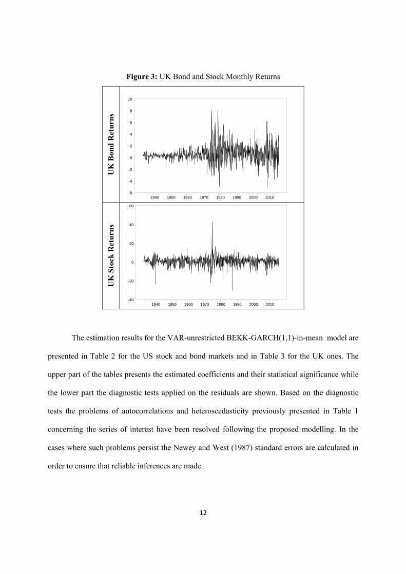
Figures 2 and 3 also provide evidence for time varying variances for bond and stock

returns in both countries. Noteworthy is that since the mid-70s the bond variability seems to have

increased significantly. This is true both in the case of the US bond market (Figure 2) as well as

11  

the UK one (Figure 3). Moreover, the distribution of these is fat-tailed because excess kurtosis is

greater than zero. These results are more pronounced on stock compared to bond returns. In view

of this, adopting the VAR(p)-BEKK-GARCH(1,1)-in-mean model in our analysis emerges as an

appropriate choice in order to take into account all of the above mentioned characteristics and the

well-known risk-return relationship in finance literature.

Figure 2: US Bond and Stock Monthly Returns

US

Bon

d R

etu

rns

US

Sto

ck R

etu

rns

1900 1920 1940 1960 1980 2000-10

-5

0

5

10

15

1900 1920 1940 1960 1980 2000-40

-20

0

20

40

60

12  

Figure 3: UK Bond and Stock Monthly Returns

UK

Bon

d R

etu

rns

UK

Sto

ck R

etu

rns

The estimation results for the VAR-unrestricted BEKK-GARCH(1,1)-in-mean model are

presented in Table 2 for the US stock and bond markets and in Table 3 for the UK ones. The

upper part of the tables presents the estimated coefficients and their statistical significance while

the lower part the diagnostic tests applied on the residuals are shown. Based on the diagnostic

tests the problems of autocorrelations and heteroscedasticity previously presented in Table 1

concerning the series of interest have been resolved following the proposed modelling. In the

cases where such problems persist the Newey and West (1987) standard errors are calculated in

order to ensure that reliable inferences are made.

1940 1950 1960 1970 1980 1990 2000 2010-6

-4

-2

0

2

4

6

8

10

1940 1950 1960 1970 1980 1990 2000 2010-40

-20

0

20

40

60

13  

Table 2: Summary of results

USA NVIX GOV INTERMED NATDIS SecMkts War Unclass

Bond market Returns

- +

Stock market Returns

- +

Bond market Volatility

- -

Stock market Volatility

+ + +

Covariance + + UK

NVIX GOV INTERMED NATDIS SecMkts War Unclass Bond market Returns

Stock market Returns

- -

Bond market Volatility

- + + -

Stock market Volatility

+ +

Covariance + + - +

We start with a bird’s eye view summary of the results presented in Table 2 before we

move to a more detailed presentation and discussion. As can be seen, from the two bond markets,

only the US market returns are positively affected by uncertainty news concerning the

corresponding security markets. Stock market returns respond positively to war news uncertainty

and negatively on INTERMED news in USA. In UK, stock returns are mainly reduced after

implied uncertainty from security market news and uncertainty from unclassified news. Bond

market volatility is reduced significantly based on NVIX and unclassified news both in the US

and the UK. Stock market volatilities in both cases are affected positively due to NATDIS news.

However, in the case of US unclassified news adds to stock market volatility while in UK case a

similar effect is brought about by INTERMED news. Finally, covariance between stock and

bond market is usually increased due to uncertainty news. However, different types of news are

responsible for this increase between stock and bond markets, across the two countries. Only in

14  

Table 3: VAR-BEKK-GARCH(1,1)-in-mean model estimation results for US data

Variable CoeffT-Stat. p-value Coeff

T-Stat. p-value Coeff

T-Stat. p-value Coeff

T-Stat. p-value Coeff

T-Stat. p-value Coeff

T-Stat. p-value Coeff

T-Stat. p-value

Const. ‐0,1423 0,45 0,2757 <0.01 0,1979 <0.01 0,1664 <0.01 0,1092 <0.01 0,2002 <0.01 0,1120 0,04

H(1,1) 0,0574 <0.01 0,0495 <0.01 0,0542 <0.01 0,0520 <0.01 0,0562 <0.01 0,0503 <0.01 0,0553 <0.01

H(1,2) 0,0641 0,01 ‐0,0252 0,43 0,0534 0,01 0,0495 0,02 ‐0,0206 0,44 0,0483 0,01 0,0520 0,01

H(2,2) ‐0,0016 0,29 0,0018 0,23 0,0002 0,78 0,0005 0,65 0,0010 0,52 0,0002 0,89 ‐0,0005 0,70RBt-1 0,1524 <0.01 0,1552 <0.01 0,1556 <0.01 0,1551 <0.01 0,1547 <0.01 0,1527 <0.01 0,1524 <0.01

RBt-2 ‐0,0353 0,15 ‐0,0459 0,05 ‐0,0398 0,07 ‐0,0395 0,08 ‐0,0491 0,04 ‐0,0411 0,07 ‐0,0367 0,11

RBt-3 0,0291 0,20 0,0486 0,02 0,0325 0,11 0,0328 0,10 0,0464 0,04 0,0309 0,13 0,0303 0,17

RBt-4 0,0014 0,95 ‐0,0124 0,58 0,0045 0,85 0,0055 0,81 ‐0,0136 0,63 0,0048 0,83 0,0043 0,85

RBt-5 0,0055 0,79 0,0023 0,92 0,0046 0,82 0,0064 0,75 0,0000 1,00 0,0062 0,76 0,0067 0,74

RSt-1 ‐0,0028 0,58 ‐0,0027 0,62 ‐0,0039 0,41 ‐0,0035 0,47 ‐0,0015 0,77 ‐0,0032 0,50 ‐0,0042 0,38

RSt-2 ‐0,0047 0,29 ‐0,0058 0,20 ‐0,0040 0,32 ‐0,0040 0,32 ‐0,0054 0,26 ‐0,0034 0,48 ‐0,0038 0,40

RSt-3 0,0022 0,64 0,0019 0,69 0,0014 0,75 0,0009 0,84 0,0022 0,68 0,0009 0,84 0,0019 0,68

RSt-4 ‐0,0007 0,89 ‐0,0011 0,82 ‐0,0020 0,70 ‐0,0017 0,73 ‐0,0007 0,89 ‐0,0012 0,81 ‐0,0022 0,70

RSt-5 ‐0,0011 0,83 ‐0,0033 0,52 ‐0,0017 0,73 ‐0,0015 0,75 ‐0,0036 0,48 ‐0,0014 0,76 ‐0,0020 0,66

Exog. Indicator t‐1

0,0133 0,06 ‐0,1153 <0.01 ‐0,0300 0,13 ‐1,0277 0,15 0,0236 <0.01 ‐0,0232 0,07 0,0098 0,15

Const. 1,0362 0,06 0,2201 0,48 0,3413 <0.01 0,2934 0,14 0,4577 0,03 0,1624 0,12 0,3845 <0.01

H(1,1) 0,0034 0,96 0,0508 0,51 ‐0,0068 0,90 0,0096 0,87 0,0614 0,41 ‐0,0054 0,92 ‐0,0102 0,86

H(1,2) 0,0186 0,26 ‐0,0026 0,86 0,0109 0,01 0,0032 0,79 0,0076 0,63 0,0042 0,56 0,0144 0,19

H(2,2) ‐0,0233 0,44 ‐0,0152 0,52 ‐0,0101 0,48 ‐0,0123 0,53 ‐0,0273 0,37 0,0011 0,93 ‐0,0116 0,52RBt-1 0,2903 <0.01 0,2858 <0.01 0,2799 <0.01 0,2812 <0.01 0,2926 <0.01 0,2760 <0.01 0,2850 <0.01

RBt-2 0,0035 0,93 0,0286 0,49 0,0045 0,91 0,0069 0,86 0,0269 0,52 0,0046 0,91 0,0070 0,87

RBt-3 0,0968 0,02 0,0861 0,05 0,0921 0,03 0,0867 0,03 0,0949 0,03 0,0916 0,03 0,0960 0,02

RBt-4 0,0006 0,99 0,0118 0,78 0,0084 0,85 0,0074 0,86 0,0069 0,87 0,0079 0,86 0,0046 0,92

RBt-5 0,1083 0,01 0,1222 0,01 0,1102 0,01 0,1071 0,01 0,1176 0,01 0,1122 0,01 0,1091 0,01

RSt-1 0,2370 <0.01 0,2465 <0.01 0,2372 <0.01 0,2383 <0.01 0,2425 <0.01 0,2392 <0.01 0,2383 <0.01

RSt-2 ‐0,0491 0,03 ‐0,0616 <0.01 ‐0,0459 0,02 ‐0,0453 0,02 ‐0,0656 0,00 ‐0,0469 0,03 ‐0,0474 0,02

RSt-3 ‐0,0035 0,88 ‐0,0023 0,92 ‐0,0077 0,72 ‐0,0078 0,72 0,0014 0,95 ‐0,0072 0,75 ‐0,0043 0,85

RSt-4 0,0277 0,16 0,0200 0,32 0,0273 0,16 0,0275 0,17 0,0185 0,40 0,0287 0,15 0,0293 0,15

RSt-5 0,0759 <0.01 0,0843 <0.01 0,0744 <0.01 0,0754 <0.01 0,0829 <0.01 0,0772 <0.01 0,0768 <0.01

Exog. Indicator t‐1

‐0,0368 0,16 0,1595 0,43 ‐0,2315 0,02 ‐1,7943 0,43 ‐0,0806 0,18 0,3670 <0.01 ‐0,0302 0,09

c11 1,1662 <0.01 ‐0,0675 0,14 0,0924 <0.01 0,0975 <0.01 ‐0,1069 <0.01 0,1148 <0.01 0,5317 <0.01

c21 ‐0,6100 0,32 1,0126 <0.01 0,1709 0,42 0,4097 0,11 0,7394 <0.01 0,1927 0,26 ‐0,0399 0,82

c22 0,0423 0,88 0,0000 1,00 0,8825 <0.01 0,9695 <0.01 0,0000 1,00 0,8866 <0.01 0,7275 <0.01

α11 0,3649 <0.01 0,3770 <0.01 0,3634 <0.01 0,3715 <0.01 0,3670 <0.01 0,3825 <0.01 0,3720 <0.01

α12 ‐0,0014 0,98 ‐0,0011 0,98 0,0197 0,65 0,0170 0,70 ‐0,0262 0,64 0,0155 0,73 0,0118 0,81

α21 0,0116 0,10 ‐0,0016 0,84 0,0123 0,01 0,0115 0,05 ‐0,0003 0,97 0,0114 0,01 0,0110 <0.01

α22 0,2685 <0.01 0,2221 <0.01 0,2659 <0.01 0,2626 <0.01 0,2301 <0.01 0,2653 <0.01 0,2738 <0.01

β11 0,9289 <0.01 0,9360 <0.01 0,9381 <0.01 0,9352 <0.01 0,9388 <0.01 0,9310 <0.01 0,9296 <0.01

β12 0,0170 0,49 0,0766 0,53 0,0005 0,97 0,0009 0,95 0,0888 0,45 0,0016 0,91 0,0064 0,68

β21 ‐0,0025 0,14 ‐0,0320 0,03 ‐0,0047 0,05 ‐0,0046 0,04 ‐0,0322 0,02 ‐0,0042 0,06 ‐0,0028 0,03

β22 0,9216 <0.01 ‐0,9523 <0.01 0,9339 <0.01 0,9334 <0.01 ‐0,9445 <0.01 0,9364 <0.01 0,9239 <0.01

κ11 ‐0,0421 <0.01 ‐0,0174 0,71 ‐0,0010 0,97 0,0747 0,95 0,0083 0,37 ‐0,0224 0,29 ‐0,0601 <0.01

κ12 0,0240 0,35 ‐0,2340 0,11 0,2472 0,02 6,8416 0,19 0,0632 0,02 0,1028 0,42 0,0257 0,18

κ22 0,0409 0,01 0,0000 1,00 ‐0,0311 0,79 8,4569 0,01 0,0000 1,00 ‐0,0382 0,64 0,0376 0,05T-Dist.

Parameter 5,2743 <0.01 5,0367 <0.01 5,1226 <0.01 5,1774 <0.01 5,0603 <0.01 5,0945 <0.01 5,2119 <0.01

Usable Obs. 1480 1480 1480 1480 1480 1480 1480

Log 

Likelihood‐6211,62 ‐6235,96 ‐6221,50 ‐6219,62 ‐6231,01 ‐6219,86 ‐6219,65

Res. Bond 

eqn.

Res. 

Stock 

eqn.

Res. Bond 

eqn.

Res. 

Stock 

eqn.

Res. Bond 

eqn.Res. Stock eqn.

Res. Bond 

eqn.

Res. Stock 

eqn.

Res. Bond 

eqn.

Res. Stock 

eqn.

Res. Bond 

eqn.

Res. 

Stock 

eqn.

Res. Bond 

eqn.

Res. Stock 

eqn.

Ljung‐Box 

Q(12)        

p‐value

0,49 0,70 0,5657 0,92 0,4221 0,86 0,4451 0,82 0,57 0,83 0,4513 0,84 0,5681 0,75

McLeod‐

Li(12)        

p‐value

0,44 0,15 0,6576 0,06 0,5702 0,13 0,5487 0,14 0,6946 0,07 0,7862 0,18 0,4724 0,11

ARCH(12) Test

p-value0,51 0,23 0,706 0,10 0,628 0,18 0,603 0,19 0,746 0,14 0,817 0,24 0,541 0,17

Exogenous SecMktst-1

RBonds-RStocks

Exogenous Wart-1

RBonds-RStocks

Exogenous Unclasst-1

RBonds-RStocks

Exogenous INTERMEDt-1 Exogenous NATDISt-1

RBonds-RStocks RBonds-RStocks RBonds-RStocks RBonds-RStocks

Bo

nd

Me

an

Retu

rn E

qu

ati

on

Sto

ck M

ean

Retu

rn E

qu

ati

on

Vari

an

ce

s-C

ovari

an

ce

eq

uati

on

sD

iag

no

sti

cs

Exogenous NVIXt-1 Exogenous GOVt-1

Notes: Bold numbers indicates statistical significance

15  

the case of the UK the bond and stock market are negatively correlated in cases of War news

uncertainty.

We now turn to a more detailed presentation and discussion of the results yielded from

estimating the mean equation for the US bond and stock returns. The well-known risk-return

result is shown, according to which investors require high return for the risk undertaken. This is

present only in the bond market but not in the stock market (see Table 3). In particular, bond

volatility coexists with high bond returns and this result does not appear to be affected when

different components of NVIX are used in the bond equation as can be deduced from coefficients

H(1,1). Stock market conditional volatility does not affect bond returns as indicated by

coefficients H(2,2) while the covariance of the two markets contributes positively to bond returns

according to NVIX as shown by coefficients H(1,2). This is the case with all the uncertainty

news components of NVIX with the exception of uncertainty news associated with government

policy (GOV) and security markets (SecMkts) as can be observed in the relevant columns of

Table 3. Generally speaking, bond returns present first order autocorrelation in most of the times,

while stock market is characterised by a higher order of autocorrelation (see coefficients of

lagged bond and stock returns). Stock returns are positively affected by bond returns with one

and five time lags while the opposite is not the case. This implies a unidirectional relationship

from bond market to stock market.

Focusing on the coefficients of the uncertainty news indicators, it appears that the effect

exerted depends on the type of news. In particular, they reveal a direct positive effect on bond

returns emanating from increased uncertainty concerning security markets news and a negative

effect from uncertainty induced by government policy news. In a similar manner, stock market

returns are positively affected by uncertainty induced by War news and negatively affected by

16  

intermediation news implied uncertainty. Worth mentioning is that for both stock and bond

markets the aggregate index of NVIX does not indicate any significant impact. This result

highlights the importance of disaggregating news implied uncertainty into different types and

uncertainty generating sources. Let us now turn to the direct effects of news-implied uncertainty

on variance equation of both bond and stock returns (see Variance-Covariance section of Table

3). As a general observation, an increase of the NVIX has a significant reduction on bond

variability (as implied by the negative and statistically significant coefficient k1,1) and a

significant rise on stock variability (as implied by the positive and statistically significant

coefficient k2,2). The former result may be attributed to the last category, entitled as “unclassified

news” when comparing the results across the different categories. While, the latter may be

attributed to NATDIS news and unclassified news also. News implied uncertainty concerning

intermediation policy and security markets bring about an significant increase in the correlation

of the two markets (see coefficient k1,2) reducing any diversification benefits for portfolio

managers.

Let us now turn to the results in the case of the UK presented in Table 4. The positive

risk-return relationship is also present to a certain degree only for the bond market but in the

cases of uncertainty news concerning government policy and intermediation this positive

relationship disappears. Additionally, the increased variability on stock market has a significant

positive effect on bond returns and this is mainly attributed to the NATDIS and SecMkts

components of NVIX. Bond returns present a notable persistence as indicated by the statistical

significance of its lagged values. Worth mentioning is the negative effect of stock returns present

under a three period delay. Unlike the US case, stock returns have a positive impact after one

period on bond returns, in only two cases: the uncertainty induced by government policy news

17  

Table 4: VAR-BEKK-GARCH(1,1)-in-mean model estimation results for UK data

Variable Coeff T-Stat. p-value Coeff

T-Stat. p-value Coeff

T-Stat. p-value Coeff

T-Stat. p-value Coeff

T-Stat. p-value Coeff

T-Stat. p-value Coeff

T-Stat. p-value

Const. 0.2153 0.05 0.1450 0.06 0.1606 0.00 0.1576 <0.01 0.1746 <0.01 0.1795 <0.01 0.1719 <0.01

H(1,1) 0.0665 0.01 0.0547 0.30 0.0504 0.17 0.0646 <0.01 0.0592 <0.01 0.0523 0.02 0.0643 <0.01

H(1,2) 0.0452 0.07 0.0586 0.68 0.0760 0.22 0.0430 0.02 0.0440 <0.01 0.0560 0.01 0.0465 <0.01

H(2,2) 0.0017 0.04 0.0010 0.62 0.0013 0.38 0.0017 0.02 0.0020 0.04 0.0013 0.25 0.0014 0.10RBt-1 0.2556 <0.01 0.2558 <0.01 0.2572 <0.01 0.2597 <0.01 0.2603 <0.01 0.2563 <0.01 0.2576 <0.01

RBt-2 ‐0.0423 0.09 ‐0.0408 0.14 ‐0.0375 0.09 ‐0.0487 0.01 ‐0.0472 0.02 ‐0.0479 0.02 ‐0.0413 0.02

RBt-3 0.0861 <0.01 0.0789 0.03 0.0800 <0.01 0.0879 <0.01 0.0885 <0.01 0.0875 <0.01 0.0861 <0.01

RSt-1 ‐0.0018 0.64 0.0001 0.97 ‐0.0002 0.97 ‐0.0016 0.68 ‐0.0020 0.60 ‐0.0013 0.74 ‐0.0011 0.78

RSt-2 0.0039 0.26 0.0038 0.45 0.0045 0.27 0.0043 0.23 0.0034 0.37 0.0037 0.30 0.0037 0.28

RSt-3 ‐0.0110 0.02 ‐0.0106 0.01 ‐0.0113 <0.01 ‐0.0115 0.01 ‐0.0112 0.01 ‐0.0112 0.02 ‐0.0114 0.01

Exog. Indicator t‐1 ‐0.0019 0.64 0.0287 0.73 0.0075 0.84 ‐0.8199 0.15 ‐0.0070 0.34 ‐0.0020 0.85 ‐0.0002 0.97

Const. 1.1013 0.06 0.2009 0.93 0.4091 0.21 0.4468 0.04 0.7320 <0.01 0.3242 0.05 0.7538 <0.01

H(1,1) 0.0221 0.74 0.0170 0.97 0.0769 0.65 0.0313 0.53 0.0344 0.46 0.0550 0.46 0.0245 0.56

H(1,2) 0.0074 0.50 ‐0.0014 0.99 0.0117 0.39 0.0083 0.43 0.0073 0.38 0.0092 0.26 0.0064 0.17

H(2,2) 0.0259 0.69 0.0750 0.84 0.0520 0.60 0.0140 0.65 0.0128 0.69 0.0414 0.45 0.0309 0.35

RBt-1 0.1301 0.11 0.2735 0.01 0.2393 <0.01 0.1299 0.06 0.1279 0.08 0.1324 0.08 0.1395 0.09

RBt-2 0.1753 0.06 0.1353 0.52 0.1685 0.14 0.1821 0.03 0.1663 0.04 0.1551 0.07 0.1819 0.07

RBt-3 0.0608 0.53 ‐0.0612 0.69 ‐0.0140 0.88 0.0642 0.43 0.0505 0.57 0.0221 0.82 0.0622 0.47

RSt-1 0.0023 0.94 0.0122 0.83 0.0027 0.93 0.0033 0.90 0.0009 0.97 0.0094 0.72 0.0005 0.98

RSt-2 ‐0.0709 0.01 ‐0.0590 0.38 ‐0.0533 0.07 ‐0.0692 0.01 ‐0.0724 0.01 ‐0.0730 0.01 ‐0.0723 0.01

RSt-3 ‐0.0075 0.78 0.0026 0.93 0.0026 0.92 ‐0.0058 0.83 ‐0.0051 0.86 ‐0.0067 0.81 ‐0.0101 0.72

Exog. Indicator t‐1 ‐0.0263 0.29 0.3762 0.40 ‐0.3494 0.08 ‐0.2355 0.95 ‐0.1430 0.05 0.1626 0.16 ‐0.0360 0.04

c11 0.4919 <0.01 ‐0.0050 0.91 ‐0.0745 <0.01 0.0052 0.49 0.0109 0.64 0.0066 0.70 0.2276 0.00

c21 ‐0.5413 0.15 3.3201 0.26 ‐3.5622 <0.01 0.0821 0.75 0.9869 <0.01 1.1098 0.02 ‐0.2116 0.31

c22 1.0893 0.06 ‐0.0001 1.00 ‐0.4312 0.61 1.1950 <0.01 ‐0.2393 0.80 0.4260 0.68 0.8914 <0.01

α11 0.3026 0.00 0.3178 <0.01 0.3231 <0.01 0.3024 <0.01 0.3102 <0.01 0.3196 <0.01 0.3048 <0.01

α12 0.1557 0.46 ‐0.3943 0.86 ‐0.1269 0.75 0.1684 0.33 0.1364 0.22 0.0515 0.75 0.1856 0.28

α21 0.0003 0.92 0.0031 0.37 0.0024 0.41 0.0000 0.99 ‐0.0019 0.75 0.0013 0.77 0.0012 0.75

α22 0.3211 <0.01 0.3598 0.42 0.4017 <0.01 0.3254 <0.01 0.3173 <0.01 0.2831 <0.01 0.3223 <0.01

β11 0.9551 <0.01 0.9608 <0.01 0.9583 <0.01 0.9582 <0.01 0.9599 <0.01 0.9575 <0.01 0.9563 <0.01

β12 ‐0.0303 0.52 0.9656 0.65 0.7258 0.01 ‐0.0418 0.30 ‐0.0263 0.23 ‐0.0032 0.93 ‐0.0337 0.35

β21 0.0004 0.56 ‐0.0061 0.77 ‐0.0072 0.21 0.0002 0.77 0.0013 0.30 0.0001 0.94 0.0003 0.61

β22 0.9250 <0.01 ‐0.6799 0.43 ‐0.5258 0.08 0.9210 <0.01 0.9275 <0.01 0.9320 <0.01 0.9242 <0.01

κ11 ‐0.0175 <0.01 0.0420 0.51 0.0752 <0.01 2.2409 <0.01 ‐0.0074 0.23 ‐0.0140 0.09 ‐0.0230 <0.01

κ12 0.0307 0.03 ‐0.3310 0.73 0.2968 0.58 12.2269 0.03 0.0123 0.78 ‐0.3743 0.03 0.0475 0.01

κ22 ‐0.0038 0.86 0.0000 0.99 1.3620 0.00 15.4887 <0.01 0.0737 0.86 0.0225 0.95 0.0144 0.50

T‐Dist. Parameter 5.0556 <0.01 4.5929 <0.01 4.5119 <0.01 5.0735 <0.01 4.9718 <0.01 4.9301 <0.01 4.9666 <0.01

Usable Observations 996 996 996 996 996 996 996

Log Likelihood ‐4078.89 ‐4119.77 ‐4114.49 ‐4077.50 ‐4083.51 ‐4078.48 ‐4079.73

Res. Bond 

eqn.

Res. 

Stock 

eqn.

Res. Bond 

eqn.

Res. 

Stock 

eqn.

Res. Bond 

eqn.

Res. Stock 

eqn.

Res. Bond 

eqn.

Res. Stock 

eqn.

Res. Bond 

eqn.

Res. Stock 

eqn.

Res. Bond 

eqn.

Res. 

Stock 

eqn.

Res. Bond 

eqn.

Res. Stock 

eqn.

Ljung‐Box Q(12)      

p‐value0.49 0.28 0.25 0.35 0.30 0.25 0.39 0.14 0.32 0.28 0.32 0.26 0.40 0.28

McLeod‐Li(12)        

p‐value0.62 0.75 0.80 <0.01 0.75 <0.01 0.74 0.50 0.68 0.75 0.65 0.56 0.68 0.75

ARCH(12) Test p-value

0.60 0.75 0.79 <0.01 0.72 <0.01 0.73 0.51 0.68 0.75 0.65 0.54 0.68 0.75

RBonds-RStocks RBonds-RStocks

Exogenous NVIXt-1 Exogenous GOVt-1 Exogenous INTERMEDt-1 Exogenous NATDISt-1 Exogenous SecMktst-1 Exogenous Wart-1

Bo

nd

Mean

Retu

rn E

qu

ati

on

Sto

ck M

ean

Retu

rn E

qu

ati

on

Va

ria

nc

es

-Co

va

rian

ce e

qu

ati

on

sD

iag

no

sti

cs

Exogenous Unclasst-1

RBonds-RStocks RBonds-RStocks RBonds-RStocks RBonds-RStocks RBonds-RStocks

Notes: Bold numbers indicates statistical significance

18  

and by intermediation policy news. Furthermore, the NATDIS and SecMkts components present

a significant positive effect on stock returns in a two time-lag specification. When it comes to the

direct effects of news-implied indicators on bond returns and in line with the US case, there are

no significant results. Nevertheless, negative effects on stock returns can be observed because of

security markets and unclassified factors-stemming uncertainty news. Just as in the case of the

US result, the NVIX exerts a negative and statistically significant effect on bond volatility that is

mainly attributed to the unclassified news factor. However, positive effects on bond volatility are

based on the effects of the intermediation and NATDIS components. The same applies when

examining the stock volatility. When examining the covariance effects of uncertainty news on

the UK case, it can be argued that the positive sign of NVIX coefficient on the covariance

equation may be attributed to the NATDIS and unclassified news components. Notably, the

correlation between the two markets is significantly reduced over the war-invoked news. This

latter result implies substantial diversification benefits between the two markets during war

periods. As far as the other coefficients in the variance equations are concerned, it can be

observed that both the stock and bond markets present a similar high volatility persistence

(compare the β11 to the β22 coefficients). Moreover, the α11 coefficients can in broad terms be

characterised as being higher in magnitude in US case compared to UK. While the α22

coefficients are, lower in the US versus the UK markets. This implies that the impact of news on

bond variability is higher in US compared to UK and the opposite for the impact of news on

stock variability (compare in Tables 3 and 4 the magnitude of the α11 and α22 coefficients

respectively).

19  

4. CONCLUDING REMARKS

The effects of news based uncertainty on the stock-bond covariance, their returns, and

their variances were the focus of the paper. To this effect, the news implied volatility index –

NVIX- was used. To allow for different effects that depend on the source of uncertainty, the

index was also decomposed into its six sub-indices that account for uncertainty emanating from

war and conflict, securities markets, natural disasters, government and intermediation policy as

well as unclassified uncertainty (Manela and Moreira, 2017). Uncertainty news may trigger a

capital movement from risky assets to more safe assets, i.e a flight-to-quality effect. Using VAR

methodology and a multivariate GARCH-in-mean framework that allows the modelling of the

variance with the covariance, we investigated the effect of uncertainty news on bond and stock

returns and their variances. Moreover, their time varying correlation was also examined in this

framework. In a nutshell, our findings indicate a positive risk return relationship for US bond

market and to a lesser extend in the case of the British bond market. Stock returns were found to

influence negatively bond market returns in both countries and, interestingly, the effect is

unidirectional only in the case of the USA. Bond returns are positively influenced by the

increased uncertainty concerning security markets news and negatively influenced from

uncertainty induced by government policy news. No effect is traced on UK bond returns. When it

comes to the effects exerted by NVIX and its constituent components the findings are mixed.

This should not come as a surprise since different news can and do affect in different ways the

bond and stock markets. The results reported herein seem to corroborate this intuitive

expectation. A more prominent result is provoked on bond and stock variability by the

uncertainty news in case of the US. More specifically, the negative effect of NVIX on bond

variability is attributed to unclassified news while the positive effect on stock variability is also

20  

laid on unclassified news and NATDIS news. Albeit appreciably feebler, this result applies in the

UK but the sign of the effect is more dependent on the type of uncertainty news. Bond returns are

positively influenced by the increased uncertainty concerning security markets news and

negatively influenced from uncertainty induced by government policy news. No effect is traced

on UK bond returns. Correlation between the two markets is found to be increased significantly

over specific type of uncertainty news for both UK and US. However, in case of UK uncertainty

news about war trigger diversification benefits implied by the appearance of a negative

correlation between stock and bond market.

 

21  

REFERENCES

Andersson, M., Krylova, E., Vahamaa, S. 2008. Why does the correlation between stock and

bond returns vary over time? Applied Financial Economics 18, 139-151

Apergis, N., M. Bonato, R. Gupta and C. Kyei. 2017. Does geopolitical risks predict stock

returns and volatility of leading defense companies? Evidence from a nonparametric

approach. Defence and Peace Economics doi.org/10.1080/10242694.2017.1292097

Asgharian, H., Christiansen, C., Hou, A.J., 2016. Macro-finance determinants of the long-run

stock-bond correlation: The DCC-MIDAS specification, Journal of Financial

Econometrics 14 (3), 617-642.

Asgharian, H., Christiansen, C., Hou, A.J., 2015. Effects of macroeconomic uncertainty on the

stock and bond markets, Finance Research Letters 13, 10-16.

Aslam, F. and H-G. Kang. 2015. How different terrorist attacks affect stock markets, Defence

and Peace Economics 26(6), 634-648

Aslanidis, N., and C. Christiansen. 2012. Smooth Transition Patterns in the Realized Stock-Bond

Correlation. Journal of Empirical Finance 19 (4), 454–464

Aslanidis, N. and C. Christiansen 2014. Quantiles of the realized stock–bond correlation and

links to the macroeconomy. Journal of Empirical Finance 28, 321–331

Baele, L., G. Bekaert and K. Inghelbrecht (2010) The determinants of stock and bond return

comovements, Review of Financial Studies 23(6), 2374-2428

Baur, D. and B. Lucey. 2009. Flights and contagion. An empirical analysis of stock-bond

correlations. Journal of Financial Stability 5: 339-352.

Bauwens, L., S. Laurent and J. Rombouts. 2006. Multivariate GARCH models: a survey. Journal

of Applied Econometrics 21:79–109.

Brune, A., T. Hens, O. Rieger and M. Wang 2015. The war puzzle: contradictory effects of

international conflicts on stock markets, International Review of Economics 62:1–21

Chang, C. L., and Hsueh, P. L. 2013. An investigation of the flight-to-quality effect: Evidence

from Asia-Pacific countries. Emerging Markets Finance and Trade 49, 53–69.

Christiansen, C. 2010. Decomposing European bond and equity volatility, International Journal

of Finance and Economics 15(2), 105-122.

Connolly, R., Stivers C., Sun L. 2005. Stock market uncertainty and the stock–bond return

relation. Journal of Financial and Quantitative Analysis 40, 161–194

22  

Connolly, R., Stivers C., Sun L. 2007. Commonality in the time-variation of stock-stock and

stock-bond return comovements. Journal of Financial Markets 40, 192-218

Dacjman, S. 2012. Comovement between stock and bond markets and the flight-to-quality

during financial market turmoil– A case of the Eurozone countries most affected by

sovereign debt crisis of 2010–2011, Applied Economics Letters 19, 1655–1662.

Dimic, N., Kiviaho, J., Pijak, V., Äijö, J., 2016. Impact of financial market uncertainty and

macroeconomic factors on stock-bond correlation in emerging markets. Research in

International Business and Finance 36, 41-51.

Durand, R. B., Junker, M., and Szimayer, A. 2010. The flight-to-quality effect: A copula-based

analysis, Accounting and Finance 50, 281–299.

Engle, R.F., Kroner, K., 1995. Multivariate simultaneous GARCH. Econometric Theory, 11,

122–150.

Guidolin, M., La Ferrara, E., 2010. The economic effects of violent conflict: evidence from asset

market reactions. Journal of Peace Research, 47, 671-684

Gulko, L. 2002. Decoupling. Journal of Portfolio Management 28, 59–66

Ilmanen, A. 2003. Stock–bond correlations. Journal of Fixed Income 13, 55–66

Kaplanski, G., Levy, H., 2010. Sentiment and stock prices: The case of aviation disasters.

Journal of Financial Economics 95, 174–201.

Kim, S., Moshirian F., Wu E. 2006. Evolution of international stock and bond market integration:

Influence of the European Monetary Union. Journal of Banking and Finance 30, 1507–

1534

Kollias, C., S. Papadamou and V. Arvanitis. 2013. Does terrorism affect the stock-bond

covariance? Evidence from European Countries, Southern Economic Journal 79(4), 832–

848

Li, L. 2002. Correlation of stock and bond returns. Working Paper, Yale University

Li, L. 2004. Macroeconomic factors and the correlation of stock and bond returns. Proceeding of

the 2004 American Finance Association Meeting

Li, X., Zou, L. 2008. How do policy and information shocks impact co-movements of China’s T-

bond and stock markets? Journal of Banking and Finance 32, 347–359

Longin, F., Solnik, B. 1995. Is the correlation in international equity returns constant: 1960–

1990? Journal of International Money and Finance 14, 3–26

23  

Manela, A. and Moreira, A. 2017. News implied volatility and disaster concerns. Journal of

Financial Economics, 123(1), 137-162.

Newey, W. and K. West. 1987. A simple positive semi-definite, heteroscedasticity and

autocorrelation consistent covariance matrix. Econometrica 55:703–08.

Ohmi H. and T. Okimoto. 2016 Trends in stock-bond correlations, Applied Economics 48(6):

536-552

Schneider, G., Troeger, V., 2006. War and the world economy, Stock market reactions to

international conflicts. Journal of Conflict Resolution 50, 623-645.

Skintzi, V. 2017 Determinants of stock-bond market comovement in the Eurozone under model

uncertainty. MPRA Paper No. 78278

Thomadakis, A. 2012 Contagion or flight-to-quality phenomena in stock and bond returns DP

06/12 Department of Economics University of Surrey

Yang, J., Y. Zhou, and Z. Wang. 2010. Conditional co-skewness in stock and bond markets: Time

series evidence, Management Science 56, 2031–2049.

Yang J., Zhou Y. and Wang Z. 2009. The stock-bond correlation and macroeconomic conditions:

one and a half centuries of evidence. Journal of Banking and Finance 33(4), 670–680.