everything you wanted to know about deep learning for...
TRANSCRIPT
Everything you wanted to know about Deep Learning for Computer Vision but wereafraid to ask
Moacir A. Ponti, Leonardo S. F. Ribeiro, Tiago S. NazareICMC – University of Sao PauloSao Carlos/SP, 13566-590, Brazil
Email: [ponti, leonardo.sampaio.ribeiro, tiagosn]@usp.br
Tu Bui, John CollomosseCVSSP – University of Surrey
Guildford, GU2 7XH, UKEmail: [t.bui, j.collomosse]@surrey.ac.uk
Abstract—Deep Learning methods are currently the state-of-the-art in many Computer Vision and Image Processingproblems, in particular image classification. After years ofintensive investigation, a few models matured and becameimportant tools, including Convolutional Neural Networks(CNNs), Siamese and Triplet Networks, Auto-Encoders (AEs)and Generative Adversarial Networks (GANs). The field is fast-paced and there is a lot of terminologies to catch up for thosewho want to adventure in Deep Learning waters. This paperhas the objective to introduce the most fundamental conceptsof Deep Learning for Computer Vision in particular CNNs,AEs and GANs, including architectures, inner workings andoptimization. We offer an updated description of the theoreticaland practical knowledge of working with those models. Afterthat, we describe Siamese and Triplet Networks, not oftencovered in tutorial papers, as well as review the literatureon recent and exciting topics such as visual stylization, pixel-wise prediction and video processing. Finally, we discuss thelimitations of Deep Learning for Computer Vision.
Keywords-Computer Vision; Deep Learning; Image Process-ing; Video Processing
I. INTRODUCTION
The field of Computer Vision was revolutionized in thepast years (in particular after 2012) due to Deep Learningtechniques. This is mainly due to two reasons: the availabil-ity of labelled image datasets with millions of images [1],[2], and computer hardware that allowed to speed-up compu-tations. Before that, there were studies exploring hierarchicalrepresentations with neural networks such as Fukushima’sNeocognitron [3] and LeCun’s neural networks for digitrecognition [4]. Although those techniques were known toMachine Learning and Artificial Intelligence communities,the efforts of Computer Vision researchers during the 2000’swas in a different direction, in particular using approachesbased on Scale-Invariant features, Bag-of-Features, SpatialPyramids and related methods [5].
After the publication of the AlexNet Convolutional NeuralNetwork Model [6], many research communities realized thepower of such methods and, from that point on, Deep Learn-ing (DL) invaded the Visual Computing fields: ComputerVision, Image Processing, Computer Graphics. Convolu-tional Neural Networks (CNNs), Deep Belief Nets (DBNs),Restricted Boltzmann Machines (RBMs) and Autoencoders
(AEs), started appearing as a basis for state-of-the-art meth-ods in several computer vision applications (e.g. remotesensing [7], surveillance [8], [9] and re-identification [10]).The ImageNet challenge [1] played a major role in thisprocess, starting a race for the model that could beat thecurrent champion in the image classification challenge, butalso image segmentation, object recognition and other tasks.In order to accomplish that, different architectures andcombinations of DBM were employed. Also, novel types ofnetworks – such as Siamese Networks, Triplet Networks andGenerative Adversarial Networks (GANs) – were designed.
Deep Learning techniques offer an important set of meth-ods suited for tasks within the domains of digital visualcontent. It is noticeable that those methods comprise adiverse variety of models, components and algorithms thatmay be dissimilar to what one may be used to in ComputerVision. A myriad of keywords within this context makes theliterature in this field almost a different language: Featuremaps, Activation, Receptive Fields, Dropout, ReLu, Max-Pool, Softmax, SGD, Adam, FC, Generator, Discriminator,Shared Weights, etc. This can make it hard for a beginnerto understand and catch up with the recent studies.
There are DL methods we do not cover in this paper,including Deep Belief Networks (DBN), Deep BoltzmannMachines (DBM) and also those using Recurrent NeuralNetworks (RNN), Reinforcement Learning and Long short-term memory (LSTMs). We refer to [11]–[14] for DBN andDBM-related studies, and [15]–[17] for RNN-related studies.
The paper is organized as follows:
• Section II provides definitions and prerequisites.• Section III aims to present a detailed and updated
description of the DL’s main terminology, buildingblocks and algorithms of the Convolutional NeuralNetwork (CNN) since it is widely used in ComputerVision, including:
1) Components: Convolutional Layer, ActivationFunction, Feature/Activation Map, Pooling, Nor-malization, Fully Connected Layers, Parameters,Loss Function;
2) Algorithms: Optimization (SGD, Momentum,
Adam, etc.) and Training;3) Architectures: AlexNet, VGGNet, ResNet, Incep-
tion, DenseNet;4) Beyond Classification: fine-tuning, feature extrac-
tion and transfer learning.• Section IV describes Autoencoders (AEs):
1) Undercomplete AEs;2) Overcomplete AEs: Denoising and Contractive;3) Generative AE: Variational AEs
• Section V introduces Generative Adversarial Net-works (GANs):
1) Generative Models: Generator/Discriminator;2) Training: Algorithm and Loss Lunctions.
• Section VI is devoted to Siamese and Triplet Net-works:.
1) SiameseNet with contrastive Loss;2) TripletNet: with triplet Loss;
• Section VII reviews Applications of Deep Networks inImage Processing and Computer Vision, including:
1) Visual Stilization;2) Image Processing and Pixel-Wise Prediction;3) Networks for Video Data: Multi-stream and C3D.
• Section VIII concludes the paper by discussing theLimitations of Deep Learning methods for ComputerVision.
II. DEEP LEARNING: PREREQUISITES AND DEFINITIONS
The prerequisites needed to understand Deep Learningfor Computer Vision includes basics of Machine Learning(ML) and Image Processing (IP). Since those are out of thescope of this paper we refer to [18], [19] for an introductionin such fields. We also assume the reader is familiar withLinear Algebra and Calculus, as well as Probability andOptimization — a review of those topics can be found inPart I of Goodfellow et al. textbook on Deep Learning [20].
Machine learning methods basically try to discover amodel (e.g. rules, parameters) by using a set of input datapoints and some way to guide the algorithm in order to learnfrom this input. In supervised learning, we have examplesof expected output, whereas in unsupervised learning someassumption is made in order to build the model. However,in order to achieve success, it is paramount to have agood representation of the input data, i.e. a good set offeatures that will produce a feature space in which analgorithm can use its bias in order to learn. One of themain ideas of Deep learning is to solve the problem offinding this representation by learning it from the data: itdefines representations that are expressed in terms of other,simpler ones [20]. Another is to assume that depth (in termsof successive representations) allows learning a sequence ofparallel instructions that transforms an initial input vector,mapping one space to another.
Deep Learning often involves learning hierarchical repre-sentations using a series of layers that operate by processingan input generating a series of representations that arethen given as input to the next layer. By having spaces ofsufficiently high dimensionality, such methods are able tocapture the scope of the relationships found in the originaldata so that it finds the “right” representation for the taskat hand [21]. This can be seen as separating the multiplemanifolds that represent data via a series of transformations.
III. CONVOLUTIONAL NEURAL NETWORKS
Convolutional Neural Networks (CNNs or ConvNets)are probably the most well known Deep Learning modelused to solve Computer Vision tasks, in particular im-age classification. The basic building blocks of CNNs areconvolutions, pooling (downsampling) operators, activationfunctions, and fully-connected layers, which are essentiallysimilar to hidden layers of a Multilayer Perceptron (MLP).Architectures such as AlexNet [6], VGG [22], ResNet [23]and GoogLeNet [24] became very popular, used as subrou-tines to obtain representations that are then offered as inputto other algorithms to solve different tasks.
We can write this network as a composition of a sequenceof functions fl(.) (related to some layer l) that takes as inputa vector xl and a set of parameters Wl, and outputs a vectorxl+1:
f(x) = fL (· · · f2(f1(x1,W1);W2) · · · ),WL)
x1 is the input image, and in a CNN the most charac-teristic functions fl(.) are convolutions. Convolutions andother operators works as building blocks or layers of aCNN: activation function, pooling, normalization and linearcombination (produced by the fully connected layer). In thenext sections we will describe each one of those buildingblocks.
A. Convolutional Layer
A layer is composed of a set of filters, each to beapplied to the entire input vector. Each filter is nothing buta matrix k × k of weights (or values) wi. Each weight is aparameter of the model to be learned. We refer to [18] foran introduction about convolution and image filters.
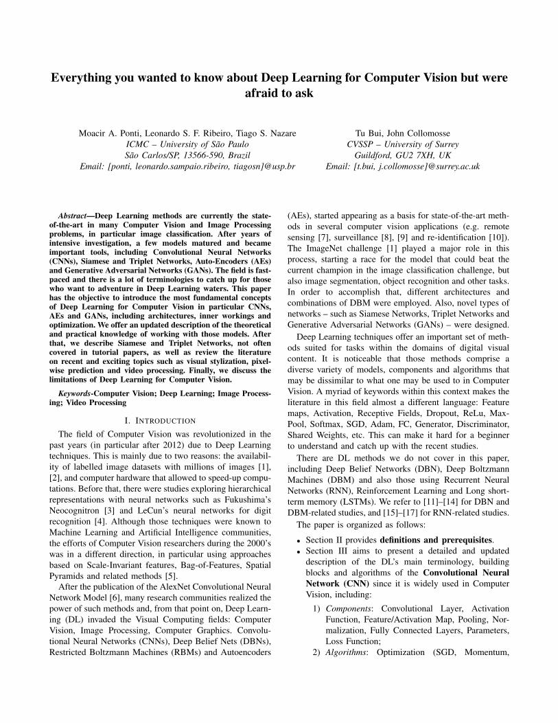
Each filter will produce what can be seen as an affinetransformation of the input. Another view is that each filterproduces a linear combination of all pixel values in aneighbourhood defined by the size of the filter. Each regionthat the filter processes is called local receptive field: anoutput value (pixel) is a combination of the input pixelsin this local receptive field (see Figure 1). That makes theconvolutional layer different from layers of an MLP forexample; in a MLP each neuron will produce a single outputbased on all values from the previous layer, whereas in aconvolutional layer, an output value f(i, x, y) is based on
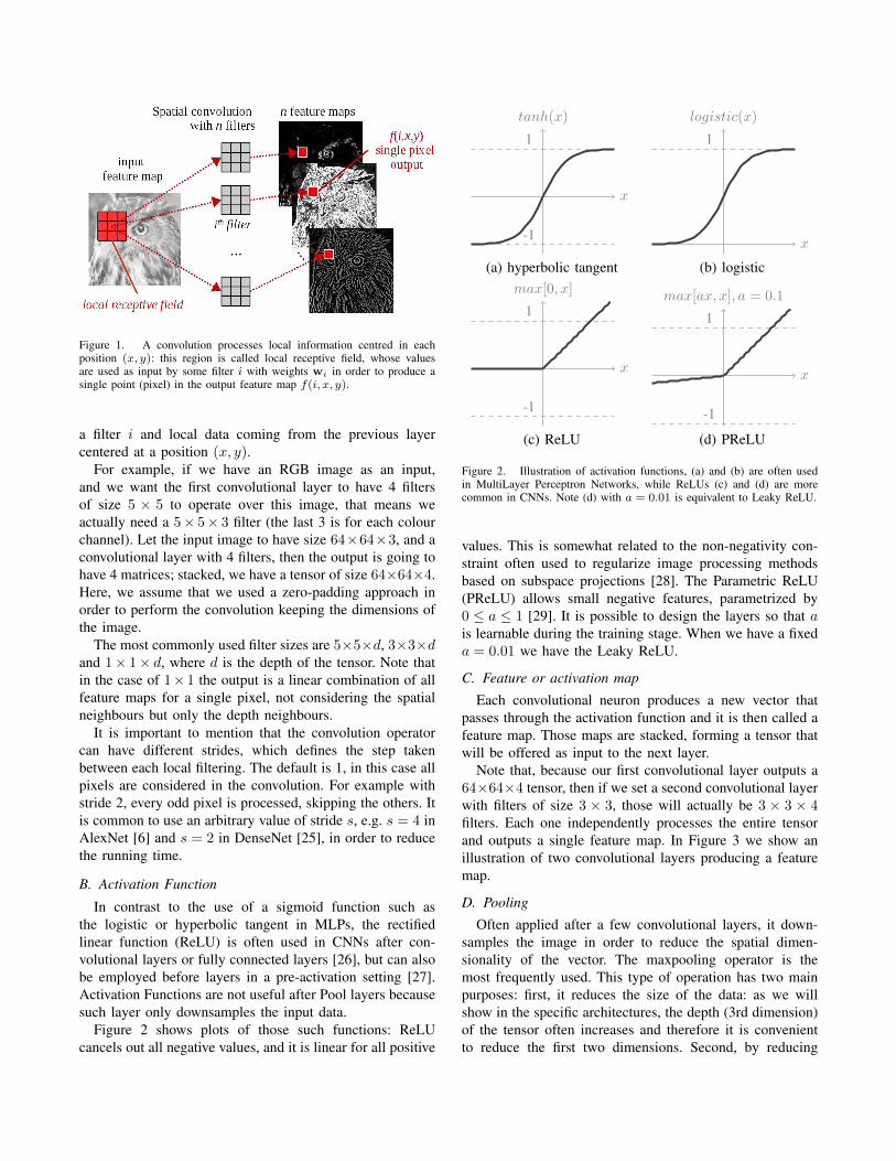
Figure 1. A convolution processes local information centred in eachposition (x, y): this region is called local receptive field, whose valuesare used as input by some filter i with weights wi in order to produce asingle point (pixel) in the output feature map f(i, x, y).
a filter i and local data coming from the previous layercentered at a position (x, y).
For example, if we have an RGB image as an input,and we want the first convolutional layer to have 4 filtersof size 5 × 5 to operate over this image, that means weactually need a 5× 5× 3 filter (the last 3 is for each colourchannel). Let the input image to have size 64×64×3, and aconvolutional layer with 4 filters, then the output is going tohave 4 matrices; stacked, we have a tensor of size 64×64×4.Here, we assume that we used a zero-padding approach inorder to perform the convolution keeping the dimensions ofthe image.
The most commonly used filter sizes are 5×5×d, 3×3×dand 1× 1× d, where d is the depth of the tensor. Note thatin the case of 1× 1 the output is a linear combination of allfeature maps for a single pixel, not considering the spatialneighbours but only the depth neighbours.
It is important to mention that the convolution operatorcan have different strides, which defines the step takenbetween each local filtering. The default is 1, in this case allpixels are considered in the convolution. For example withstride 2, every odd pixel is processed, skipping the others. Itis common to use an arbitrary value of stride s, e.g. s = 4 inAlexNet [6] and s = 2 in DenseNet [25], in order to reducethe running time.
B. Activation Function
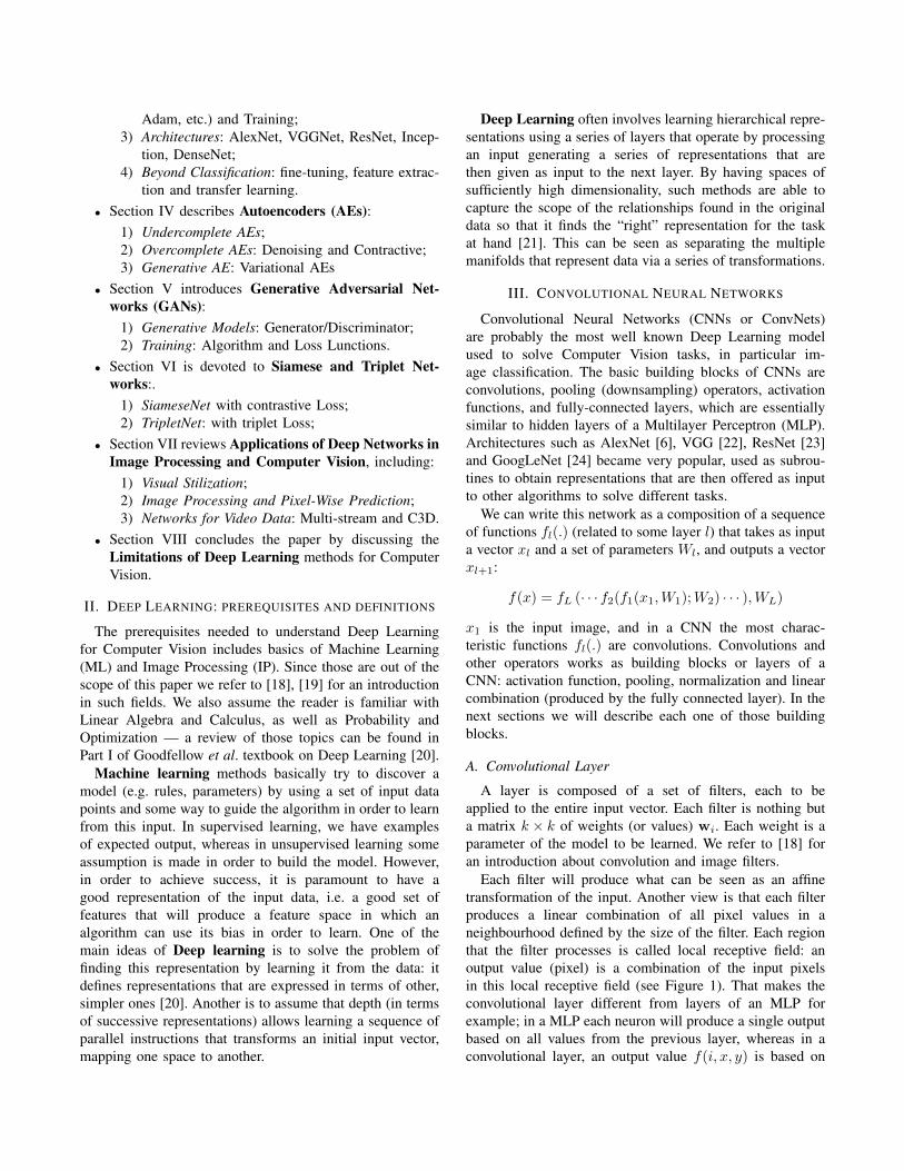
In contrast to the use of a sigmoid function such asthe logistic or hyperbolic tangent in MLPs, the rectifiedlinear function (ReLU) is often used in CNNs after con-volutional layers or fully connected layers [26], but can alsobe employed before layers in a pre-activation setting [27].Activation Functions are not useful after Pool layers becausesuch layer only downsamples the input data.
Figure 2 shows plots of those such functions: ReLUcancels out all negative values, and it is linear for all positive
x
1
-1
tanh(x)
x
1
logistic(x)
(a) hyperbolic tangent (b) logistic
x
max[0, x]
1
-1
x
max[ax, x], a = 0.1
1
-1
(c) ReLU (d) PReLU
Figure 2. Illustration of activation functions, (a) and (b) are often usedin MultiLayer Perceptron Networks, while ReLUs (c) and (d) are morecommon in CNNs. Note (d) with a = 0.01 is equivalent to Leaky ReLU.
values. This is somewhat related to the non-negativity con-straint often used to regularize image processing methodsbased on subspace projections [28]. The Parametric ReLU(PReLU) allows small negative features, parametrized by0 ≤ a ≤ 1 [29]. It is possible to design the layers so that ais learnable during the training stage. When we have a fixeda = 0.01 we have the Leaky ReLU.
C. Feature or activation map
Each convolutional neuron produces a new vector thatpasses through the activation function and it is then called afeature map. Those maps are stacked, forming a tensor thatwill be offered as input to the next layer.
Note that, because our first convolutional layer outputs a64×64×4 tensor, then if we set a second convolutional layerwith filters of size 3 × 3, those will actually be 3 × 3 × 4filters. Each one independently processes the entire tensorand outputs a single feature map. In Figure 3 we show anillustration of two convolutional layers producing a featuremap.
D. Pooling
Often applied after a few convolutional layers, it down-samples the image in order to reduce the spatial dimen-sionality of the vector. The maxpooling operator is themost frequently used. This type of operation has two mainpurposes: first, it reduces the size of the data: as we willshow in the specific architectures, the depth (3rd dimension)of the tensor often increases and therefore it is convenientto reduce the first two dimensions. Second, by reducing
Figure 3. Illustration of two convolutional layers, the first with 4 filters 5× 5× 3 that gets as input an RGB image of size 64× 64× 3, and producesa tensor of feature maps. A second convolutional layer with 5 filters 3× 3× 4 gets as input the tensor from the previous layer of size 64× 64× 4 andproduces a new 64× 64× 5 tensor of feature maps. The circle after each filter denotes an activation function, e.g. ReLU.
the image size it is possible to obtain a kind of multi-resolution filter bank, by processing the input in differentscale spaces. However, there are studies in favour to discardthe pooling layers, reducing the size of the representationsvia a larger stride in the convolutional layers [30]. Also,because generative models (e.g. variational AEs, GANs, seeSections IV and V) shown to be harder to train with poolinglayers, there is probably a tendency for future architecturesto avoid pooling layers.
E. Normalization
It is common also to apply normalization to both theinput data and after convolutional layers. In input datapreprocessing it is common to apply a z-score normalization(centring by subtracting the mean and normalizing thestandard deviation to unity) as described by [31], whichcan be seen as a whitening process. For layer normalizationthere are different approaches such as the channel-wise layernormalization, that normalizes the vector at each spatiallocation in the input map, either within the same featuremap or across consecutive channels/maps, using L1-norm,L2-norm or variations.
In AlexNet architecture (2012) [6] the Local ResponseNormalization (LRN) is used: for every particular input pixel(x, y) for a given filter i, we have a single output pixelfi(x, y), which is normalized using values from adjacentfeature maps j, i.e. fj(x, y). This procedure incorporatesinformation about outputs of other kernels applied to thesame position (x, y).
However, more recent methods such as GoogLeNet [24]and ResNet [23] do not mention the use of LRN. Instead,they use Batch normalization (BN) [32]. We describe BN inSection III-J.
F. Fully Connected Layer
After many convolutional layers, it is common to includefully connected (FC) layers that work in a way similar to ahidden layer of an MLP in order to learn weights to classifythe representation. In contrast to a convolutional layer, forwhich each filter produces a matrix of local activation values,the fully connected layer looks at the full input vector,producing a single scalar value. In order to do that, it takes asinput the reshaped version of the data coming from the lastlayer. For example, if the last layer outputs a 4 × 4 × 40tensor, we reshape it so that it will be a vector of size1 × (4 × 4 × 40) = 1 × 640. Therefore, each neuron inthe FC layer will be associated with 640 weights, producinga linear combination of the vector. In Figure 4 we show anillustration of the transition between a convolutional layerwith 5 feature maps with size 2×2 and an FC layer with mneurons, each producing an output based on f(xTw + b),in which x is the feature map vector, w are the weightsassociated with each neuron of the fully connected layer,and b are the bias terms.
The last layer of a CNN is often the one that outputs theclass membership probabilities for each class c using logisticregression:
P (y = c|x;w; b) = softmaxc(xTw + b) =
exTwc+bc∑
j exTwj+bj
,
where y is the predicted class, x is the vector coming fromthe previous layer, w and b are respectively the weights andthe bias associated with each neuron of the output layer.
G. CNN architecture and its parameters
Typical CNNs are organized using blocks of convolutionallayers (Conv) followed by an activation function (AF), even-tually pooling (Pool) and then a series of fully connected
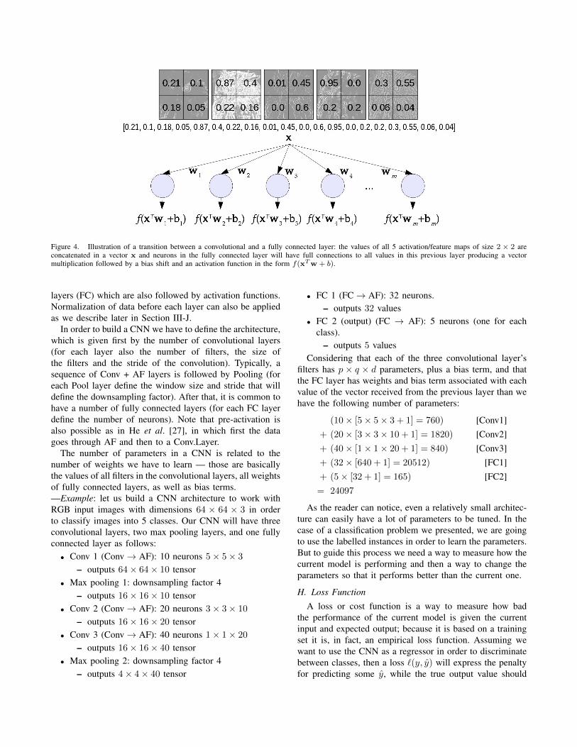
Figure 4. Illustration of a transition between a convolutional and a fully connected layer: the values of all 5 activation/feature maps of size 2 × 2 areconcatenated in a vector x and neurons in the fully connected layer will have full connections to all values in this previous layer producing a vectormultiplication followed by a bias shift and an activation function in the form f(xTw + b).
layers (FC) which are also followed by activation functions.Normalization of data before each layer can also be appliedas we describe later in Section III-J.
In order to build a CNN we have to define the architecture,which is given first by the number of convolutional layers(for each layer also the number of filters, the size ofthe filters and the stride of the convolution). Typically, asequence of Conv + AF layers is followed by Pooling (foreach Pool layer define the window size and stride that willdefine the downsampling factor). After that, it is common tohave a number of fully connected layers (for each FC layerdefine the number of neurons). Note that pre-activation isalso possible as in He et al. [27], in which first the datagoes through AF and then to a Conv.Layer.
The number of parameters in a CNN is related to thenumber of weights we have to learn — those are basicallythe values of all filters in the convolutional layers, all weightsof fully connected layers, as well as bias terms.—Example: let us build a CNN architecture to work withRGB input images with dimensions 64 × 64 × 3 in orderto classify images into 5 classes. Our CNN will have threeconvolutional layers, two max pooling layers, and one fullyconnected layer as follows:• Conv 1 (Conv→ AF): 10 neurons 5× 5× 3
– outputs 64× 64× 10 tensor• Max pooling 1: downsampling factor 4
– outputs 16× 16× 10 tensor• Conv 2 (Conv→ AF): 20 neurons 3× 3× 10
– outputs 16× 16× 20 tensor• Conv 3 (Conv→ AF): 40 neurons 1× 1× 20
– outputs 16× 16× 40 tensor• Max pooling 2: downsampling factor 4
– outputs 4× 4× 40 tensor
• FC 1 (FC→ AF): 32 neurons.– outputs 32 values
• FC 2 (output) (FC → AF): 5 neurons (one for eachclass).
– outputs 5 valuesConsidering that each of the three convolutional layer’s
filters has p × q × d parameters, plus a bias term, and thatthe FC layer has weights and bias term associated with eachvalue of the vector received from the previous layer than wehave the following number of parameters:
(10× [5× 5× 3 + 1] = 760) [Conv1]+ (20× [3× 3× 10 + 1] = 1820) [Conv2]+ (40× [1× 1× 20 + 1] = 840) [Conv3]+ (32× [640 + 1] = 20512) [FC1]+ (5× [32 + 1] = 165) [FC2]= 24097
As the reader can notice, even a relatively small architec-ture can easily have a lot of parameters to be tuned. In thecase of a classification problem we presented, we are goingto use the labelled instances in order to learn the parameters.But to guide this process we need a way to measure how thecurrent model is performing and then a way to change theparameters so that it performs better than the current one.
H. Loss Function
A loss or cost function is a way to measure how badthe performance of the current model is given the currentinput and expected output; because it is based on a trainingset it is, in fact, an empirical loss function. Assuming wewant to use the CNN as a regressor in order to discriminatebetween classes, then a loss `(y, y) will express the penaltyfor predicting some y, while the true output value should

be y. The hinge loss or max-margin loss is an exampleof this type of function that is used in the SVM classifieroptimization in its primal form. Let fi ≡ fi(xj ,W ) be ascore function for some class i given an instance xj and aset o parameters W , then the hinge loss is:
`(h)j =
∑c 6=yj
max(0, fc − fyj + ∆
),
where class yj is the correct class for the instance j. Thehyperparameter ∆ can be used so that when minimizing thisloss, the score of the correct class needs to be larger than theincorrect class scores by ∆ at least. There is also a squaredversion of this loss, called squared hinge loss.
For the softmax classifier, often used in neural networks,the cross-entropy loss is employed. Minimizing the cross-entropy between the estimated class probabilities:
`(ce)j = − log
(efyj∑k e
fk
), (1)
in which k = 1 · · ·C is the index of each neuron for theoutput layer with C neurons, one per class.
This function takes a vector of real-valued scores to avector of values between zero and one with unitary sum.There is an interesting probabilistic interpretation of mini-mizing Equation 1 in which it can be seen as minimizing theKullback-Leibler divergence between two class distributionsin which the true distribution has zero entropy (since it hasa single probability 1) [33]. Also, we can interpret it asminimizing the negative log likelihood of the correct class,which is related to the Maximum Likelihood Estimation.
The full loss of some training set (a finite batch of data)is the average of the instances’ xj outputs, f(xj ;W ), giventhe current set of all parameters W :
L(W ) =1
N
N∑j=1
` (yj , f(xj ;W )) .
We now need to minimize L(W ) using some optimizationmethod.
– Regularization: there is a possible problem withusing only the loss function as presented. This is becausethere might be many similar W for which the model is ableto correctly classify the training set, and this can hamperthe process of finding good parameters via minimization ofthe loss, i.e. make it difficult to converge. In order to avoidambiguity of solution, it is possible to add a new term thatpenalizes undesired situations, which is called regularization.The most common regularization is the L2-norm: by addinga sum of squares, we want to discourage individually largeweights:
R(W ) =∑k
∑l
W 2k,l
We then expand the loss by adding this term, weighted bya hyperparameter λ to control the regularization influence:
L(W ) =1
N
N∑j=1
` (yj , f(xj ;W )) + λR(W ).
The parameter λ controls how large the parameters in Ware allowed to grow, and it can be found by cross-validationusing the training set.
I. Optimization Algorithms
After defining the loss function, we want to adjust theparameters so that the loss is minimized. The GradientDescent is the standard algorithm for this task, and thebackpropagation method is used to obtain the gradient forthe sequence of weights using the chain rule. We assume thereader is familiar with the fundamentals of both GradientDescent and backpropagation, and focus on the particularcase of CNNs.
Note that L(W ) is based on a finite dataset and because ofthat we are computing Montecarlo estimates (via randomlyselected examples) of the real distribution that generatesthe parameters. Also, recall that CNNs can have a lot ofparameters to be optimized, therefore needing to be trainedusing thousands or millions of images (many current datasetshave more than 1TB of data). But if we have millions ofexamples to be used in the optimization, then the GradientDescent is not viable, since this algorithm has to computethe gradient for all examples individually. The difficulty hereis easy to see because if we try to run an epoch (i.e. a passthrough all the data) we would have to load all the examplesinto a limited memory, which is not possible. Alternativesto overcome this problem are described below, including theSGD, Momentum, AdaGrad, RMSProp and Adam.
– Stochastic Gradient Descent (SGD): one possiblesolution to accelerate the process is to use approximatemethods that goes through the data in samples composedof random examples drawn from the original dataset. Thisis why the method is called Stochastic Gradient Descent:now we are not inspecting all available data at a time, but asample, which adds uncertainty in the process. We can evencompute the Gradient Descent using a single example at atime ( a method often used in streams or online learning).However, in practice, it is common to use mini-batcheswith size B. By performing enough iterations (each iterationwill compute the new parameters using the examples in thecurrent mini-batch), we assume it is possible to approximatethe Gradient Descent method.
Wt+1 = Wt − ηB∑j=1
∇L(W ;xBj ),
in which η is the learning rate parameter: a large η willproduce larger steps in the direction of the gradient, whilea small value produces a smaller step in the direction of the
gradient. It is common to set a larger initial value for η, andthen exponentially decrease it as a function of the iterations.
In fact, SGD is a rough approximation, producing a non-smooth convergence. Because of that, variants were pro-posed to compensate for that, such as the Adaptive Gradient(AdaGrad) [34], Adaptive learning rate (AdaDelta) [35] andAdaptive moment estimation (Adam) [36]. Those variantsbasically use the ideas of momentum and normalization, aswe describe below.
– Momentum: adds a new variable α to control thechange in the parameters W . It creates a momentum thatprevents the new parameters Wt+1 from deviating too muchfrom the previous direction:
Wt+1 = Wt + α(Wt −Wt−1) + (1− α) [−η∇L(Wt)] ,
where L(Wt) is the loss computed using some examplesusing the current parameters Wt (often a mini-batch). Notethat the magnitude of the step for the iteration t+ 1 now isalso constrained by the step taken in the iteration t.
– AdaGrad: works by putting more weight on rare orinfrequent parameters. It creates a history of how much agiven parameter already changed the loss, accumulating theindividual gradients gt+1 = gt +∇L(Wt)
2. Then, the nextstep is now scaled/normalized for each parameter:
Wt+1 = Wt −η∇L(Wt)
2
√gt+1 + ε
,
since this historical gradient is computed feature-wise, theinfrequent features will have more influence in the nextgradient descent step.
– RMSProp: computes running averages of recentgradient magnitudes and normalizes using these average sothat loosely gradient values are normalized. It is similarto AdaGrad, but here gt is computed by an exponentiallydecaying average and not the simple sum of gradients:
gt+1 = γgt + (1− γ)∇L(Wt)2
g is called the second order moment of ∇L (don’t confuseit with momentum). The final parameter update is given byadding the momentum:
Wt+1 = Wt + α(Wt −Wt−1) + (1− α)
[− η∇L(Wt)√
gt+1 + ε
],
– Adam: uses an idea that is similar to AdaGrad andRMSProp, but the momentum is used for the first and secondorder moment so now we have α and γ to control themomentum of respectively W and g. The influence of bothdecays over time so that the step size decreases when itapproaches minimum. We use an auxiliary variable m forclarity:
mt+1 = αt+1gt + (1− αt+1)∇L(Wt)
mt+1 =mt+1
1− αt+1
m is called the first order moment of ∇L (don’t confuse itwith momentum) and m is m after applying the decayingfactor. Then we need to compute the gradients g to use inthe normalization:
gt+1 = γt+1gt + (1− γt+1)∇L(Wt)2
gt+1 =gt+1
1− γt+1
g is called the second order moment of ∇L (again, don’tconfuse it with momentum). The final parameter update isgiven by:
Wt+1 = Wt −ηmt+1√gt+1 + ε
J. Tricks for Training CNNs
– Initialization: random initialization of weights isimportant to the convergence of the network. The Gaussiandistribution N (µ, σ) is often used to produce the randomnumbers. However, for models with more than 8 convo-lutional layers, the use of a fixed standard deviation (e.g.σ = 0.01) as in [6] was shown to hamper convergence.Therefore, when using rectifiers as activation functions it isrecommended to use µ = 0, σ =
√2/nl, where nl is the
number of connections of a response of a given layer l; aswell as initializing all bias parameters to zero [29],.
– Minibatch size: due to the need of using SGDoptimization and variants, one must define the size of theminibatch of images that is going to be used to train themodel taking into account memory constraints but alsothe behaviour of the optimization algorithm. For example,while a small batch size can make the loss minimizationmore difficult, the convergence speed of SGD degradeswhen increasing the minibatch size for convex objectivefunctions [37]. In particular, assuming SGD converges inT iterations, then minibatch SGD with batch size B runs inO(1/
√BT + 1/T ).
However, increasing B is important to reduce the varianceof the SGD updates (by using the average of the loss), andthis, in turn, allows you to take bigger step-sizes [38]. Also,larger minibatches are interesting when using GPUs, since itgives better throughput by performing backpropagation withdata reuse using matrix multiplication (instead of severalvector-matrix multiplications), and needing fewer transfersto the GPU. Therefore, it can be an advantage to choosethe batch size so that it fully occupies the GPU memoryand choose the largest experimentally found step size. Whilepopular architectures (as we will discuss in Section III-K)use from 32 to 256 examples in the batch size, a recentpaper used a linear scaling rule for adjusting learning ratesas a function of minibatch size, also adding a warmupscheme with large step-sizes in the first few epochs to avoidoptimization problems. By using 256 GPUs and a batch sizeof 8192, Goyal et al. [39] were able to train a ResidualNetwork with 50 layers with the ImageNet in 1 hour.

– Dropout: a technique proposed by [40] that, duringthe forward pass of the network training stage, randomlydeactivate neurons of a layer with some probability p (inparticular from FC layers). It has relationships with the Bag-ging ensemble method [41] because, at each iteration of themini-batch SGD, the dropout procedure creates a randomlydifferent network by subsampling the activations, which istrained using backpropagation. This method became knownas a form of regularization that prevents the network tooverfit. In the test stage, the dropout is turned off, and theactivations are re-scaled by p to compensate those activationsthat were dropped during the training stage.
– Batch normalization (BN): also used as a regularizer,it normalizes the a layer activations at each batch of inputdata by maintaining the mean activation close to 0 (cen-tering) and the activation standard deviation close to 1, andusing parameters γ and β to produce a linear transformationof the normalized vector, i.e.:
BNγ,β(xi) = γ
(xi − µB√σ2B + ε
)+ β, (2)
in which γ and β are parameters that can be learned duringthe backpropagation stage [32]. This allows for example toadjust the normalization, and even restore the data back toits un-normalized form, i.e. when γ =
√σ2B and β = µB .
BN became a standard in the recent years, often replacingthe use of both regularization and dropout (e.g. ResNet [23]and Inception V3 [42] and V4).
– Data-augmentation: as mentioned previously, CNNsoften have a large set of parameters to be optimized, requir-ing a huge number of training examples. Because it is veryhard to have a dataset with sufficient examples, it is commonto employ some type of data augmentation. Also, usuallyimages in the same dataset often have similar illuminationconditions, a low variance of rotation, pose, etc. Therefore,one can augment the training dataset by many operations inorder to produce 5 to 10 times more examples [43] such as:(i) cropping images in different positions — note that CNNsoften have a low-resolution image input (e.g. 224 × 224)so we can find several cropped versions of an image withhigher resolution; (ii) flipping images horizontally — andalso vertically if it makes sense, e.g. in case of remotesensing and astronomical images; (iii) adding noise [44];(iv) creating new images by using PCA as in the Fancy PCAproposed by [6]. Note that augmentation must be performedpreserving the labels.
– Pre-processing: the input data can be pre-processedin several ways: (i) compute the average image for the wholetraining data and subtracting it from each image; (ii) z-score normalization (as mentioned in Normalization), (iii)PCA whitening that first tries to decorrelate the data byprojecting zero-centered original data into the eigenbasis,and then takes the data in the eigenbasis and divides everydimension by the eigenvalue to normalize the scale.
– Fine-tuning: when you have a small dataset it canbe a challenge to train a CNN. Even data augmentationcan be insufficient since augmentation will create perturbedversions of the same images. In this case, it is very usefulto use a model already trained in a large dataset (forexample the ImageNet dataset [1]), with initial weights thatwere already learned. To obtain a trained model, adapt itsarchitecture to your dataset and re-enter training phase usingsuch dataset is a process called fine-tuning. Because it ofteninvolves the use of a different dataset we discuss this in moredetail in Section III-L about Transfer Learning and FeatureExtraction.
K. CNN Architectures for Image Classification
There are many proposed CNN architectures for im-age classification. We chose to cover those that containsignificant differences starting with AlexNet, all designedfor image classification (1000 classes) of ImageNet Chal-lenge [1]. We refer also to Fukushima’s Neocognitron [3]and LeNet [4], both important studies for the history ofDeep Learning in Computer Vision. We first describe eacharchitecture and later we show an overall comparison inTable I.
– AlexNet [6]: was the champion model in ImageNetChallenge 2012. With ∼ 60 million parameters and 650000neurons, AlexNet was originally designed in two branchesallowing parallel processing. It uses Local Response nor-malization, maxpooling with overlapping (window size 3,stride 2), a batch size of 128 examples, momentum of 0.9weight decay of 0.0005. They initialized the weights usingGaussian-distributed random values with fixed σ = 0.01,and bias to 1 for the 2nd, 4th and 5th convolutional layers,and bias to 0 for the remaining layers. The learning ratewas initialized to 0.01 and arbitrarily dividing this learningrate by 10 three times during the training stage. In Figure 5we show a diagram of the layers and compare it with theVGG-16, the latter is described next.
– VGG-Net [22]: this architecture was developed toincrease the depth while making all filters with at most3 × 3 size. The rationale behind this is that 2 consecutive3× 3 conv. layers will have an effective receptive field of5 × 5, and 3 of such layers an effective receptive field of7× 7 when combining the feature maps. The authors claimthat stacking 3 conv. layers with 3 × 3 filters instead ofusing just one with filter size 7 × 7 has the advantage ofincorporating more rectification layers, making the decisionfunction more discriminative. Also, it incorporates 1 × 1conv. layers that perform a linear projection of a position(x, y) across all feature maps in a given layer. There aretwo most commonly used versions of this CNN: VGG-16and VGG-19, respectively with 16 weight layers and 19weight layers. In Figure 5 we show a diagram of the layersof VGG-16 and compare it with the AlexNet.

AlexNet architecture22
4×
224
imag
e
Con
v1:
96fil
ters
11×
11
Max
pool
ing
1
Con
v2:
256
filte
rs5×
5
Max
pool
ing
2
Con
v3:
384
filte
rs3×
3
Con
v4:
385
filte
rs3×
3
Con
v5:
256
filte
rs3×
3
Max
pool
ing
3
FC1
4096
neur
ons
FC2
4096
neur
ons
FC3
outp
ut10
00ne
uron
s
224×
224
imag
e
Con
v1:
64fil
ters
3×
3
Con
v2:
64fil
ters
3×
3
Max
pool
ing
1
Con
v3:
128
filte
rs3×
3
Con
v4:
128
filte
rs3×
3
Max
pool
ing
2
Con
v5:
256
filte
rs3×
3
Con
v6:
256
filte
rs3×
3
Con
v7:
256
filte
rs1×
1
Max
pool
ing
3
Con
v8:
512
filte
rs3×
3
Con
v9:
512
filte
rs3×
3
Con
v10:
512
filte
rs1×
1
Max
pool
ing
4
Con
v11:
512
filte
rs3×
3
Con
v12:
512
filte
rs3×
3
Con
v13:
512
filte
rs1×
1
Max
pool
ing
5
FC1
4096
neur
ons
FC2
409
6ne
uron
s
FC3
outp
ut10
00ne
uron
s
VGG-16 architecture
Figure 5. Outline of CNN architectures: AlexNet with variable filter sizes(top), and VGG-16 with fixed 3× 3 filter sizes (bottom).
During training, the batch size used is 256. LRN isnot used since it shows no classification improvement butincreased running time. Maxpooling uses window size 2 andstride 2. Training was regularized by weight decay using L2regularization λ = 0.0005, and dropout with 0.5 ratio forthe first two FC layers. Learning rate and initialization weresimilar to those used in AlexNet, but all bias parameterswere set to 0 and an initialization followed also a pretrainingapproach.
– Residual Networks (ResNet) [23]: the study describ-ing ResNets raises the question of whether we really getbetter networks by simply stacking more layers. At the timeof the publication VGG-19 was considered “very deep”, andthe authors show that, although depth seems to be correlatedwith better results, in practice, when increasing the numberof layers, the accuracy first saturates and then starts todegrade rapidly and fail to even work in the training set,therefore underfitting.
He et al. [23] claim that this could, in fact, be anoptimization problem, and propose the use of residualblocks for networks with 34 to 152 layers. Those blocksare designed to preserve the characteristics of the originalvector x before its transformation by some layer fl(x) byskipping weight layers and performing the sum fl(x) + x.In Figure 6 we show a diagram of three different versionsof such blocks, and in Figure 7 the ResNet architecturewith 34 layers that uses the residual block and residualblock with pooling. The authors claim that, because thegradient is an additive term, it is unlikely to vanish even withmany layers. Interestingly, this architecture does not containany FC hidden layers. After the last convolution layer, anAverage pooling is computed followed by the output layer.
The bottleneck blocks (Figure 6-(c)) are designed tocompress the depth of the input feature map via 1 × 1
x
weights
weights
f(x)
+
f(x) + x
ReLU
ReLU
identity
x
weights + pooling
weights
f(x)
+
f(x) + p(x)
ReLU
ReLU
pooling
x with d = 256
64, 1× 1
64, 3× 3
256, 1× 1
f(x)
+
f(x) + x
ReLU
ReLU
ReLU
(a) residual block (b) with pooling (c) bottleneck
Figure 6. Modules to preserve the characteristics the original vector(identity) allows the vector to skip weight layers, typically skipping 2 layers:(a) the original vector x before its modification by weights is summed withits transformed version f(x); (b) when some layer also include poolingoperation, the dashed line indicates the original vector needed pooling tobe summed; (c) in the bottleneck module illustrated, the depth (256) of theinput is reduced by the first 1×1 layer of 64 filters and then restored backto 256 by the third layer.
convolutions with a reduced number of filters, and thenrestore its depth by adding another layer of containing anumber of filters 1×1 equal to the depth of the input featuremap. The bottleneck blocks are used in ResNet with 50, 101and 152 layers. For example, the ResNet-50 is basically theResNet-34 replacing all residual blocks (each containing 2weight layers) with bottleneck blocks (each has 3 weightlayers).
For the ImageNet training the authors adopt only BatchNormalization (BN) without regularization, dropout or nor-malization; data augmentation was performed using crops,horizontal flip and Fancy PCA; they also preprocessed theimages by average subtraction. The batch size used was 256and the remaining parameters are similar to the previouslydescribed methods as shown in Table I.
– GoogLeNet [24] and Inception [42]: the GoogLeNetas proposed by [24] and the VGGNet [22] achieved similarperformances in the 2014 ImageNet challenge [2]. However,the GoogLeNet received attention due to its architecturebased on modules called Inception (see Figure 8). Laterimprovements in this model are called Inception archi-tectures such as the Inception V3 presented by [42], inwhich the authors also discuss design principles of CNNarchitectures including: (i) gentle decrease of representationsize from input to output; (ii) use of higher dimensionalrepresentations per layer (and consequently more activationmaps); (iii) use of lower dimensional embeddings using1× 1 convolutions before spatial convolutions; (iv) balanceof width (number of filters per layer) and depth (number oflayers).
Recently, the same authors incorporated ideas fromResNets, producing many variants including Inception V4and Inception-ResNet [45]. Here, for didactic purposes, we

224×
224
imag
e
Con
v1:
64
,7×
7,pl/2
Max
pool
ing/2
Con
v2:
64,3×
3
Con
v3:
64,3×
3
Con
v4:
64,3×
3
Con
v5:
64,3×
3
Con
v6:
64,3×
3
Con
v7:
64,3×
3
Con
v8:
128,3×
3,pl/2
Con
v9:
128,3×
3
Con
v10:
128,3×
3
Con
v11:
128,3×
3
Con
v12:
128,3×
3
Con
v13:
128,3×
3
Con
v14:
128,3×
3
Con
v15:
128,3×
3
Con
v16:
256,3×
3,pl/2
Con
v17:
256,3×
3
Con
v18:
256,3×
3
Con
v19:
256
,3×
3
Con
v20:
256
3×
3
Con
v21:
256
,3×
3
Con
v22:
256,3×
3
Con
v23:
256,3×
3
Con
v24:
256,3×
3
Con
v25:
256,3×
3
Con
v26:
256,3×
3
Con
v27:
256,3×
3
Con
v28:
512,3×
3,pl/2
Con
v29:
512,
3×
3
Con
v30:
512,3×
3
Con
v31:
512,3×
3
Con
v32:
512
3×
3
Con
v33:
512,3×
3
Ave
rage
pool
ing
FCou
tput
100
0ne
uron
s
Figure 7. Outline of ResNet-34 architecture. Solid lines indicate identity mappings skipping layers, while dashed lines indicate identity mappings withpooling in order to match the size of the representation in the layer it skips to.
x
1× 1
5× 5
1× 1
3× 3
Pool
1× 1
1× 1
Feature maps concatenation
x
1× 1
3× 3
3× 3
1× 1
3× 3
Pool
1× 1
1× 1
Feature maps concatenation
(a) Original Inception (b) Inception v3-1
x
1× 1
1× k
k × 1
1× k
k × 1
1× 1
1× k
k × 1
Pool
1× 1
1× 1
Feature maps concatenation
x
1× 1
3× 3
1× 3 3× 1
1× 1
1× 3 1× 3
Pool
1× 1
1× 1
Feature maps concatenation
(c) Inception v3-2 (d) Inception v3-3
Figure 8. Inception modules (a) traditional; (b) replacing the 5 × 5 bytwo 3× 3 convolutions; (c) with factorization of k× k convolution filters,(d) with expanded filter bank outputs.
focus on Inception V3 since the V4 is basically a variant ofthe previous one.
The Inception module breaks larger filters (e.g. 5 × 5,7 × 7) that are computationally expensive, into smallerconsecutive filters that have the same effective receptivefield. Note that this idea was already explored in VG-GNet. However, the Inception explores this idea stackingdifferent sequences (in parallel) of small convolutions andconcatenates the outputs of the different parallel sequences.The original Inception [24] is shown in Figure 8-(a), whilein Inception V3 it follows the design principle (iii) and
proposes to factorize a 5 × 5 convolution into two 3 × 3as in Figure 8-(b). In addition, two other modules areproposed: a factorization module for k × k convolutions asin Figure 8-(c), and an expanded filter bank to increase thedimensionality of representations as shown in Figure 8-(d).
We show the Inception V3 architecture in Figure 9: thefirst layers include regular convolution layers and pooling,followed by different Inception modules (type V3-1,2,3). Wehighlight the size of the representation in some transitionsof the network. This is important because to show thatwhile the first two dimensions shrink, the third increasesfollowing the principles (i), (ii) and (iv). Note that theInception modules type V3-2 are used with size k = 7 foran input representation of spatial size 17×17. The Inceptionmodules type V3-3, that output a concatenation of 6 featuremaps per module has the intention of increasing the depthof the feature maps in a coarser scale (spatial size 8 × 8).Although this architecture has 42 layers (considering internalconvolutions layers inside Inception modules), because ofthe factorization is has a small size in terms of parameters.
For Inception V3 the authors also employ a label-smoothing regularization (LSR) that tries to constrain thelast layer to output a non-sparse solution. Given an inputexample, let k be the index for all classes of a givenproblem, Y (k) be the ground truth for each class k, Y (k)the predicted output and P (k) a prior for each class. TheLSR can be seen as using a pair of cross-entropy losses,one that penalizes the incorrect label, and a second thatpenalizes it to deviate from the prior label distribution, i.e.(1 − γ)`(Y (k), Y (k)) + γ`(P (k), Y (k)). The parameter γcontrols the influence of the LSR and P represent the priorof a given class.
To train the network for ImageNet, they used LSR witha uniform prior, i.e. the same for all classes: P (k) =1/1000∀k for the ImageNet 1000-class problem and γ =0.1, BN is applied in both convolutional and FC layers.The optimization algorithm is the RMSProp. All otherparameters are standard. They also used gradient clippingwith threshold 2.
– DenseNet [25]: inspired by ideas from both ResNetsand Inception, the DenseNet introduces the DenseBlock,a sequence of layers where each layer l takes as input

299×
299×
3im
age
Con
v1:
32,
3×
3,s
=2
Con
v2:
32,3×
3,s
=1
Con
v3:
64
,3×
3,s
=1
Max
pool
ing
3×
3,s
=2
Con
v4:
128
filte
rs3×
3
Con
v5:
256
filte
rs3×
3
Con
v6:
256
filte
rs3×
3
Con
v7:
256
filte
rs1×
1
Ince
ptio
nV
3-1
Ince
ptio
nV
3-1
Ince
ptio
nV
3-1
Ince
ptio
nV
3-2
Ince
ptio
nV
3-2
Ince
ptio
nV
3-2
Ince
ptio
nV
3-2
Ince
ptio
nV
3-2
Ince
ptio
nV
3-3
Ince
ptio
nV
3-3
Max
pool
ing
8×
8
FC1
2048
neur
ons
FC2
outp
ut100
0ne
uron
s
35× 35× 288 17× 17× 768 8× 8× 1280 8× 8× 2048 1× 1× 2048
Figure 9. Outline of Inception V3 architecture. Convolutions do not use zero-padding except for Conv3 (in gray). The stride is indicated by s. Wehighlight the size of the representations before and after the Inception modules types, and also after the last max pooling layer.
all preceding feature maps x1,x2, · · · ,xl−1 concatenated.Thus, each layer produces an output which is a function ofall previous feature maps, i.e.:
xl = Hl ([x1,x2, · · · ,xl−1]) .
Hence, while regular networks with L layers have L con-nections, each DenseBlock (illustrated in Figure 10) has anumber of connections following an arithmetic progression,i.e. L(L+1)
2 direct connections. The DenseNet is a concate-nation of multiple inputs of Hl() into a single tensor. EachHl is composed of three operations, in sequence: batchnormalization (BN), followed by ReLU and then a 3 × 3convolution. This unusual sequence of operations is calledpre-activation unit, was introduced by He et al. [27] andhas the property of yielding a simplified derivative for eachunit that is unlikely to be canceled out, which would in turnimproves the convergence process.
Transition layers are layers between DenseBlocks com-posed of BN, a 1 × 1 Conv.Layer, followed by a 2 × 2average pooling with stride 2.
Variations of DenseBlocks: they also experimented usingbottleneck layers, in this case each DenseBlock is a sequenceof operations: BN, ReLU, 1 × 1 Conv., followed by BN,ReLU, 3 × 3 Conv. This variation is called DenseNet-B.Finally, a compression method is also proposed to reduce thenumber of feature maps at transition layers with a factor θ.When bottleneck and compression are combined they referthe model as DenseNet-BC.
Each layer has many input feature maps; if each Hl
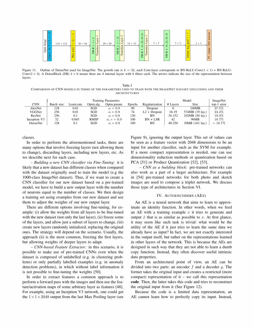
produces k feature maps, then the lth layer has k0+k×(l−1)input maps, where k0 is the number of channels in theinput image. However, the authors claim that DenseNetrequires fewer filters per layer [25]. The number filters kis a hyperparameter defined in DenseNet as the growth rate.For the ImageNet dataset k = 32 is used. We show theoutline of the DenseNet architecture used for ImageNet inFigure 11.
– Comparison and other archictectures: in order toshow an overall comparison of all architectures described,we listed the training parameters, size of the model and top1error in the ImageNet dataset for AlexNet, VGGNet, ResNet,Inception V3 and DenseNet in Table I.
Inpu
t
BN
+R
eLU
+C
onv:H
1
BN
+R
eLU
+C
onv:H
2
BN
+R
eLU
+C
onv:H
3
BN
+R
eLU
+C
onv:H
4
BN
+R
eLU
+C
onv:H
5
Tran
sitio
n(B
N+C
onv+
Pool
)
Figure 10. Illustration of a DenseBlock with 5 functions Hl and aTransition Layer.
Finally, we want to refer to another model that wasdesigned to be small, compressing the representations, theSqueezeNet [46], based on AlexNet but with 50× fewerparameters and additional compression so that it could, forexample, be implemented in embedded systems.
L. Beyond Classification: fine-tuning, feature extraction andtransfer learning
When one needs to work with a small dataset of images,it is not viable to train a Deep Network from scratch, withrandomly initialized weights. This is due to the high numberof parameters and layers, requiring millions of images,plus data augmentation. However, models such as the onesdescribed in this paper (e.g. VGGNet, ResNet, Inception),that were trained with large datasets such as the ImageNet,can be useful even for tasks other than classifying the imagesfrom that dataset. This is because the learned weights can bemeaningful for other datasets, even from a different domainsuch as medical imaging [47].
In this context, by starting with some model pre-trainedwith a large dataset, we can use the networks as FeatureExtractors [48] or even to achieve Transfer Learning [49].It is also possible to perform Fine-tuning of a pre-trainedmodel to create a new classifier with a different set of
Inpu
tIm
age
Con
v1:
16
,7×
7,s
=2
Max
pool
3×
3,s
=2
DB
-B1:
4×
6
Tran
sitio
nL
ayer
1
DB
-B2:
4×
12
Tran
sitio
nL
ayer
2
DB
-B3:
24,3
2,4
8,64
Tran
sitio
nL
ayer
3
DB
-B4:
16,3
2,3
2,48
Glo
bal
Avg
pool
7×
7
FCou
tput
100
0ne
uron
s
112× 112 56× 56 28× 28 14× 14 7× 7 7× 7 1× 1
Figure 11. Outline of DenseNet used for ImageNet. The growth rate is k = 32, each Conv.layer corresponds to BN-ReLU-Conv(1 × 1) + BN-ReLU-Conv(3× 3). A DenseBlock (DB) 4× 6 means there are 4 internal layers with 6 filters each. The arrows indicate the size of the representation betweenlayers.
Table ICOMPARISON OF CNN MODELS IN TERMS OF THE PARAMETERS USED TO TRAIN WITH THE IMAGENET DATASET (INCLUDING AND THEIR
ARCHITECTURES
Training Parameters Model ImageNetCNN Batch size Learn.rate Optm.alg. Optm.param. Epochs Regularization # Layers Size top-1 error
AlexNet 128 0.01 SGD α = 0.9 90 Dropout 8 240MB 37.5%VGGNet 256 0.01 SGD α = 0.9 74 L2 + Dropout 16-19 574MB (19 lay.) 24.4%ResNet 256 0.1 SGD α = 0.9 120 BN 34-152 102MB (50 lay.) 19.3%
Inception V3 32 0.045 RMSP α, γ = 0.9 100 BN + LSR 42 96MB 18.7%DenseNet 128 0.1 SGD α = 0.9 100 BN 40-250 30MB (161 lay.) ∼ 18.7%
classes.In order to perform the aforementioned tasks, there are
many options that involve freezing layers (not allowing themto change), discarding layers, including new layers, etc. Aswe describe next for each case.
– Building a new CNN classifier via Fine-Tuning: it islikely that a new dataset has different classes when comparedwith the dataset originally used to train the model (e.g the1000-class ImageNet dataset). Thus, if we want to create aCNN classifier for our new dataset based on a pre-trainedmodel, we have to build a new output layer with the numberof neurons equal to the number of classes. We then designa training set using examples from our new dataset and usethem to adjust the weights of our new output layer.
There are different options involving fine-tuning, for ex-ample: (i) allow the weights from all layers to be fine-tunedwith the new dataset (not only the last layer), (ii) freeze someof the layers, and allow just a subset of layers to change, (iii)create new layers randomly initialized, replacing the originalones. The strategy will depend on the scenario. Usually, theapproach (ii) is the most common, freezing the first layers,but allowing weights of deeper layers to adapt.
– CNN-based Feature Extractor: in this scenario, it ispossible to make use of pre-trained CNNs even when thedataset is composed of unlabelled (e.g. in clustering prob-lems) or only partially labelled examples (e.g. in anomalydetection problems), in which without label information itis not possible to fine-tuning the weights [50].
In order to extract features a common approach is toperform a forward pass with the images and then use the fea-ture/activation maps of some arbitrary layer as features [48].For example, using an Inception V3 network, one could getthe 1×1×2048 output from the last Max Pooling layer (see
Figure 9), ignoring the output layer. This set of values canbe seen as a feature vector with 2048 dimensions to be aninput for another classifier, such as the SVM for example.If a more compact representation is needed, one can usedimensionality reduction methods or quantization based onPCA [51] or Product Quantization [52], [53].
– CNN as a building block: pre-trained networks canalso work as a part of a larger architecture. For examplein [54] pre-trained networks for both photo and sketchimages are used to compose a triplet network. We discussthose type of architectures in Section VI.
IV. AUTOENCODERS (AES)
An AE is a neural network that aims to learn to approx-imate an identity function. In other words, when we feedan AE with a training example x it tries to generate andoutput x that is as similar as possible to x. At first glance,it may seem like such task is trivial: what would be theutility of the AE if it just tries to learn the same data wealready have as input? In fact, we are not exactly interestedin the output itself, but rather on the representations learnedin other layers of the network. This is because the AEs aredesigned in such way that they are not able to learn a dumbcopy function. Instead, they often discover useful intrinsicdata properties.
From an architectural point of view, an AE can bedivided into two parts: an encoder f and a decoder g. Theformer takes the original input and creates a restricted (morecompact) representation of it – we call this representationcode. Then, the latter takes this code and tries to reconstructthe original input from it (See Figure 12).
Because the code is a limited data representation, anAE cannot learn how to perfectly copy its input. Instead,
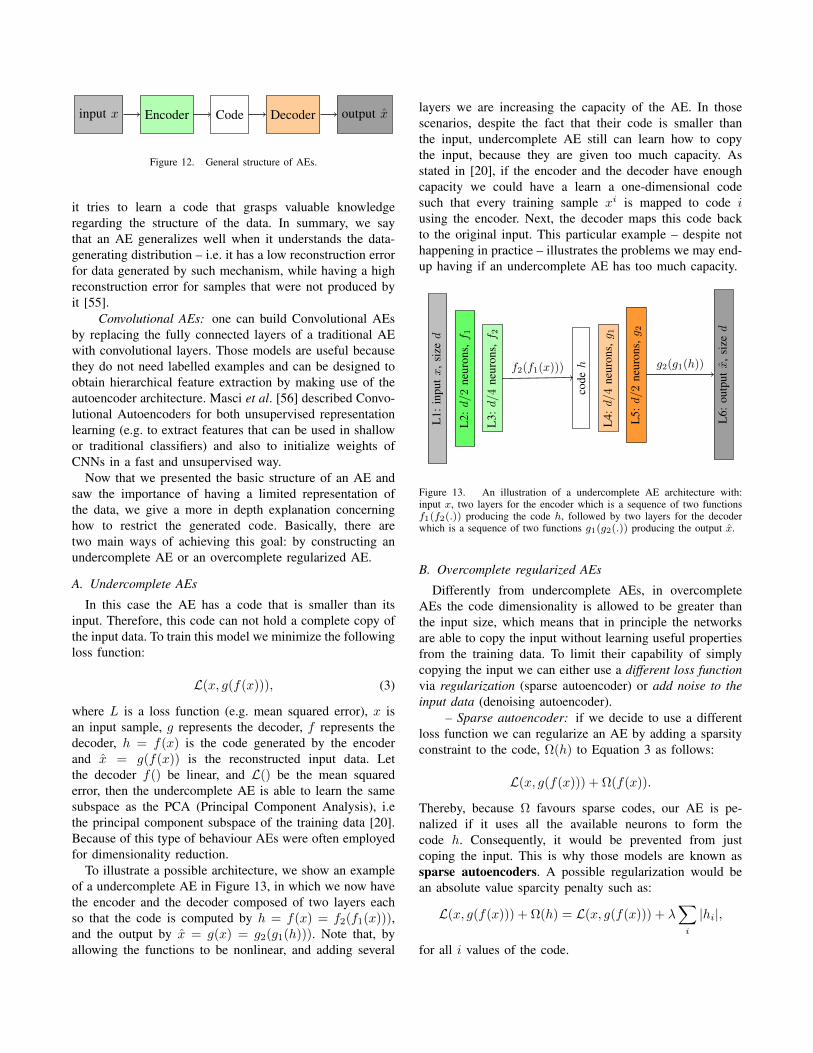
input x Encoder Code Decoder output x
Figure 12. General structure of AEs.
it tries to learn a code that grasps valuable knowledgeregarding the structure of the data. In summary, we saythat an AE generalizes well when it understands the data-generating distribution – i.e. it has a low reconstruction errorfor data generated by such mechanism, while having a highreconstruction error for samples that were not produced byit [55].
Convolutional AEs: one can build Convolutional AEsby replacing the fully connected layers of a traditional AEwith convolutional layers. Those models are useful becausethey do not need labelled examples and can be designed toobtain hierarchical feature extraction by making use of theautoencoder architecture. Masci et al. [56] described Convo-lutional Autoencoders for both unsupervised representationlearning (e.g. to extract features that can be used in shallowor traditional classifiers) and also to initialize weights ofCNNs in a fast and unsupervised way.
Now that we presented the basic structure of an AE andsaw the importance of having a limited representation ofthe data, we give a more in depth explanation concerninghow to restrict the generated code. Basically, there aretwo main ways of achieving this goal: by constructing anundercomplete AE or an overcomplete regularized AE.
A. Undercomplete AEs
In this case the AE has a code that is smaller than itsinput. Therefore, this code can not hold a complete copy ofthe input data. To train this model we minimize the followingloss function:
L(x, g(f(x))), (3)
where L is a loss function (e.g. mean squared error), x isan input sample, g represents the decoder, f represents thedecoder, h = f(x) is the code generated by the encoderand x = g(f(x)) is the reconstructed input data. Letthe decoder f() be linear, and L() be the mean squarederror, then the undercomplete AE is able to learn the samesubspace as the PCA (Principal Component Analysis), i.ethe principal component subspace of the training data [20].Because of this type of behaviour AEs were often employedfor dimensionality reduction.
To illustrate a possible architecture, we show an exampleof a undercomplete AE in Figure 13, in which we now havethe encoder and the decoder composed of two layers eachso that the code is computed by h = f(x) = f2(f1(x))),and the output by x = g(x) = g2(g1(h))). Note that, byallowing the functions to be nonlinear, and adding several
layers we are increasing the capacity of the AE. In thosescenarios, despite the fact that their code is smaller thanthe input, undercomplete AE still can learn how to copythe input, because they are given too much capacity. Asstated in [20], if the encoder and the decoder have enoughcapacity we could have a learn a one-dimensional codesuch that every training sample xi is mapped to code iusing the encoder. Next, the decoder maps this code backto the original input. This particular example – despite nothappening in practice – illustrates the problems we may end-up having if an undercomplete AE has too much capacity.
L1:
inpu
tx
,siz
ed
L2:d/2
neur
ons,f 1
L3:d/4
neur
ons,f 2
codeh
L4:d/4
neur
ons,g 1
L5:d/2
neur
ons,g 2
L6:
outp
utx
,siz
ed
f2(f1(x))) g2(g1(h))
Figure 13. An illustration of a undercomplete AE architecture with:input x, two layers for the encoder which is a sequence of two functionsf1(f2(.)) producing the code h, followed by two layers for the decoderwhich is a sequence of two functions g1(g2(.)) producing the output x.
B. Overcomplete regularized AEs
Differently from undercomplete AEs, in overcompleteAEs the code dimensionality is allowed to be greater thanthe input size, which means that in principle the networksare able to copy the input without learning useful propertiesfrom the training data. To limit their capability of simplycopying the input we can either use a different loss functionvia regularization (sparse autoencoder) or add noise to theinput data (denoising autoencoder).
– Sparse autoencoder: if we decide to use a differentloss function we can regularize an AE by adding a sparsityconstraint to the code, Ω(h) to Equation 3 as follows:
L(x, g(f(x))) + Ω(f(x)).
Thereby, because Ω favours sparse codes, our AE is pe-nalized if it uses all the available neurons to form thecode h. Consequently, it would be prevented from justcoping the input. This is why those models are known assparse autoencoders. A possible regularization would bean absolute value sparcity penalty such as:
L(x, g(f(x))) + Ω(h) = L(x, g(f(x))) + λ∑i
|hi|,
for all i values of the code.

– Denoising autoencoder: we can regularize an AE bydisturbing its input with some kind of noise. This meansthat our AE has to reconstruct an input sample x given acorrupted version of it x. Then each example is a pair (x, x)and now the loss is given by the following equation:
L(x, g(f(x))).
By using this approach we restrain our model from copy-ing the input and force it to learn to remove noise and, as aresult, to gain valuable insights on the data distribution. AEsthat use such strategy are called denoising autoencoders(DAEs).
In principle, the DAEs can be seen as MLP networks thatare trained to remove noise from input data. However, asin all AEs, learning an output is not the main objective.Therefore, DAEs aim to learn a good internal representationas a side effect of learning a denoised version of theinput [57].
– Contractive autoencoder: by regularizing the AEusing the gradient of the input x, we can learn functionsso that the code rate of change follows the rate of changein the input x. This requires a different form for Ω that nowdepends also on x such as:
Ω(x, h) = λ∑i
∥∥∥∥∂h∂x∥∥∥∥2F
,
i.e. the squared Frobenius norm of the Jacobian matrix ofpartial derivatives associated with the encoder function. Thecontractive autoencoder, or CAE, has theoretical connec-tions with denoising AEs and manifold learning. In [58] theauthors show that denoising AEs make the reconstructionfunction to resist small and finite perturbations of x, whilecontractive autoencoders make the function resist infinitesi-mal perturbations of x.
The name contractive comes from the fact that the CAEfavours the mapping of a neighbourhood of input points (xand its perturbed versions) into a smaller neighbourhood ofoutput points (thus locally contracting), warping the space.We can think of the Jacobian matrix J at a point x as alinear approximation of a nonlinear encoder f(x). A linearoperator is said to be contractive if the norm of Jx is keptless than or equal to 1 for all unit-norm of x, i.e. if itshrinks the unit sphere around each point. Therefore theCAE encourages each of the local linear operators to becomea contraction.
In addition to the contractive term, we still need tominimize the reconstruction error, which alone would leadto learning the function f() as the identity map. But thecontractive penalty will guide the learning process so that wehave most derivatives ∂f(x)
∂x approaching zero, while only afew directions with a large gradient for x that rapidly changethe code h. Those are likely the directions approximatingthe tangent planes of the manifold. These tangent directions
ideally correspond to real variations of the data. For instance,if we use images as input, then a CAE should learn tangentvectors corresponding to moving or changing parts of objects(e.g. head and legs) [59].
C. Generative Autoencoders
As mentioned previously, the autoencoders can be usedto learn manifolds in a nonparametric fashion. It is possibleto associate each of the neurons/nodes of a representationwith a tangent plane that spans the directions of variationsassociated with the difference vectors between the exampleand its neighbours [60]. An embedding associates eachtraining example with a real-valued vector position [20]. Ifwe have enough examples to cover the curvature and warpsof the target manifold, we could, for example, generate newexamples via some interpolation of such positions. In thissection we focus on generative AEs, but we also describeGenerative Adversarial Networks in this paper at Section V.
The idea of using an AE as a generative model is toestimate the density Pdata, or P (x), that generates the data.For example, in [61] the authors show that when trainingDAEs including a procedure to corrupt the data x with noiseusing a conditional distribution C(x|x), the DAE is trainedto estimate the reverse conditional P (x|x) as a side-effect.Combining this estimator with the known corruption process,they show that it is possible to obtain an estimator of P (x)through a Markov chain that alternates between samplingfrom the reconstruction distribution model P (x|x) (decode),apply the stochastic corruption procedure C(x|x) (decode),and iterate.
– Variational Autoencoders: in addition to the use ofCAEs and DAEs for generating examples, the VariationalAutoencoders (VAE) emerged as an important method ofunsupervised learning of complex distributions and used asgenerative models [62].
VAEs were introduced as a constrained version of tradi-tional autoencoders that learn an approximation of the truedistribution and are currently one of the most used generativemodels available [63], [64]. Although VAEs share littlemathematical basis with CAEs and DAEs, its structure alsocontains encoder and a decoder modules, thus resembling atraditional autoencoder. In summary, it uses latent variablesz that can be seen as a space of rules that enforces a validexample sampled from P (x). In practice, it tries to find afunction Q(z|x) (encoder) which can take a value x andgive as output a distribution over z values that are likely toproduce x.
To illustrate a training-time VAE implemented as a feed-forward network we shown a simple example in Figure 14.In our example P (x|z) is given by a Gaussian distribution,and therefore we have a set of two parameters θ = µ,Σ.Also, two loss functions are employed: (1) a Kullback-Leibler (KL) divergence LKL between the distributionsformed by the estimated parameters N (µ(x),Σ(x)) and
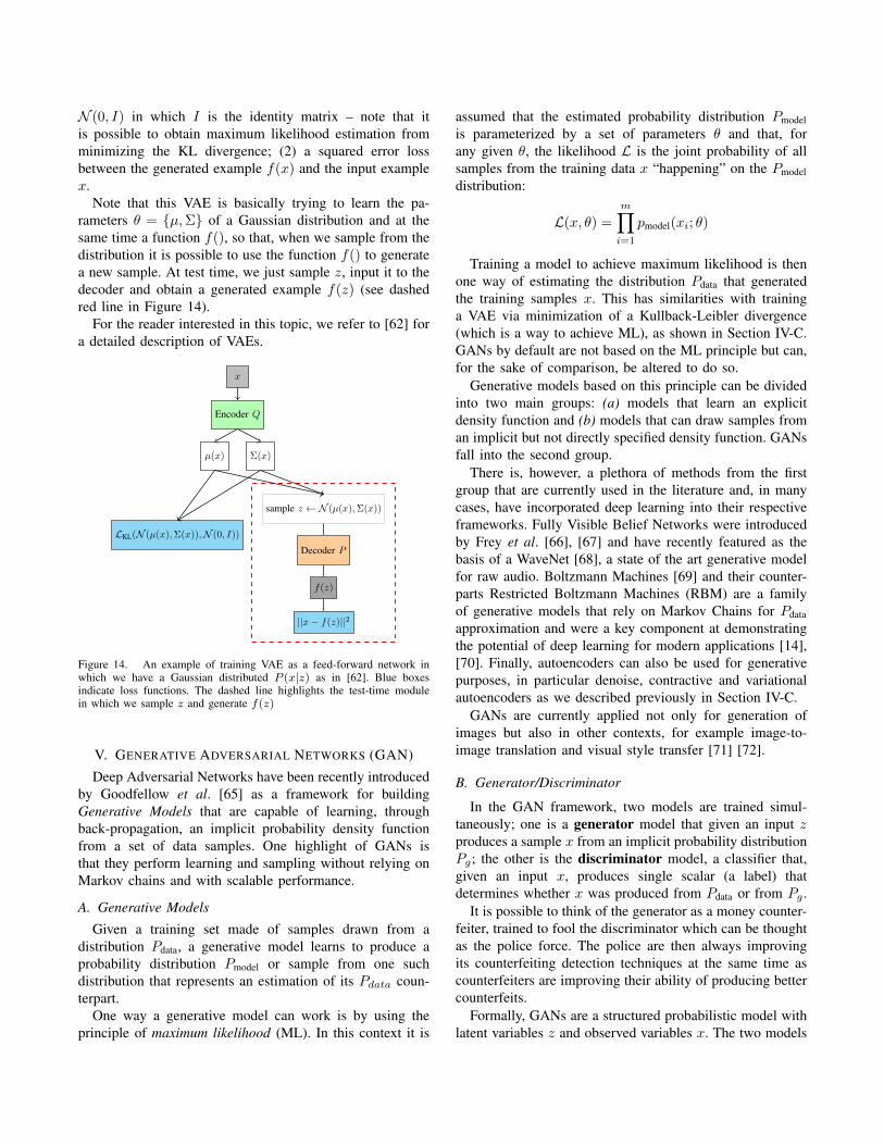
N (0, I) in which I is the identity matrix – note that itis possible to obtain maximum likelihood estimation fromminimizing the KL divergence; (2) a squared error lossbetween the generated example f(x) and the input examplex.
Note that this VAE is basically trying to learn the pa-rameters θ = µ,Σ of a Gaussian distribution and at thesame time a function f(), so that, when we sample from thedistribution it is possible to use the function f() to generatea new sample. At test time, we just sample z, input it to thedecoder and obtain a generated example f(z) (see dashedred line in Figure 14).
For the reader interested in this topic, we refer to [62] fora detailed description of VAEs.
x
Encoder Q
µ(x) Σ(x)
LKL(N (µ(x),Σ(x)),N (0, I))
sample z ← N (µ(x),Σ(x))
Decoder P
f(z)
||x− f(z)||2
Figure 14. An example of training VAE as a feed-forward network inwhich we have a Gaussian distributed P (x|z) as in [62]. Blue boxesindicate loss functions. The dashed line highlights the test-time modulein which we sample z and generate f(z)
V. GENERATIVE ADVERSARIAL NETWORKS (GAN)
Deep Adversarial Networks have been recently introducedby Goodfellow et al. [65] as a framework for buildingGenerative Models that are capable of learning, throughback-propagation, an implicit probability density functionfrom a set of data samples. One highlight of GANs isthat they perform learning and sampling without relying onMarkov chains and with scalable performance.
A. Generative Models
Given a training set made of samples drawn from adistribution Pdata, a generative model learns to produce aprobability distribution Pmodel or sample from one suchdistribution that represents an estimation of its Pdata coun-terpart.
One way a generative model can work is by using theprinciple of maximum likelihood (ML). In this context it is
assumed that the estimated probability distribution Pmodelis parameterized by a set of parameters θ and that, forany given θ, the likelihood L is the joint probability of allsamples from the training data x “happening” on the Pmodeldistribution:
L(x, θ) =
m∏i=1
pmodel(xi; θ)
Training a model to achieve maximum likelihood is thenone way of estimating the distribution Pdata that generatedthe training samples x. This has similarities with traininga VAE via minimization of a Kullback-Leibler divergence(which is a way to achieve ML), as shown in Section IV-C.GANs by default are not based on the ML principle but can,for the sake of comparison, be altered to do so.
Generative models based on this principle can be dividedinto two main groups: (a) models that learn an explicitdensity function and (b) models that can draw samples froman implicit but not directly specified density function. GANsfall into the second group.
There is, however, a plethora of methods from the firstgroup that are currently used in the literature and, in manycases, have incorporated deep learning into their respectiveframeworks. Fully Visible Belief Networks were introducedby Frey et al. [66], [67] and have recently featured as thebasis of a WaveNet [68], a state of the art generative modelfor raw audio. Boltzmann Machines [69] and their counter-parts Restricted Boltzmann Machines (RBM) are a familyof generative models that rely on Markov Chains for Pdataapproximation and were a key component at demonstratingthe potential of deep learning for modern applications [14],[70]. Finally, autoencoders can also be used for generativepurposes, in particular denoise, contractive and variationalautoencoders as we described previously in Section IV-C.
GANs are currently applied not only for generation ofimages but also in other contexts, for example image-to-image translation and visual style transfer [71] [72].
B. Generator/Discriminator
In the GAN framework, two models are trained simul-taneously; one is a generator model that given an input zproduces a sample x from an implicit probability distributionPg; the other is the discriminator model, a classifier that,given an input x, produces single scalar (a label) thatdetermines whether x was produced from Pdata or from Pg .
It is possible to think of the generator as a money counter-feiter, trained to fool the discriminator which can be thoughtas the police force. The police are then always improvingits counterfeiting detection techniques at the same time ascounterfeiters are improving their ability of producing bettercounterfeits.
Formally, GANs are a structured probabilistic model withlatent variables z and observed variables x. The two models
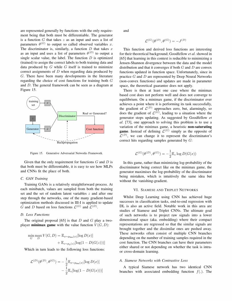
are represented generally by functions with the only require-ment being that both must be differentiable. The generatoris a function G that takes z as an input and uses a list ofparameters θ(G) to output so called observed variables x.The discriminator is, similarly, a function D that takes xas an input and uses a list of parameters θ(D) to output asingle scalar value, the label. The function D is optimized(trained) to assign the correct labels to both training data anddata produced by G while G itself is trained to minimizecorrect assignments of D when regarding data produced byG. There have been many developments in the literatureregarding the choice of cost functions for training both Gand D. The general framework can be seen as a diagram atFigure 15.
trainingset
x
x
DiscriminatorReal or Generated?
Cost functionGenerator
z
Backpropagation
Figure 15. Generative Adversarial Networks Framework.
Given that the only requirement for functions G and D isthat both must be differentiable, it is easy to see how MLPsand CNNs fit the place of both.
C. GAN Training
Training GANs is a relatively straightforward process. Ateach minibatch, values are sampled from both the trainingset and the set of random latent variables z and after onestep through the networks, one of the many gradient-basedoptimization methods discussed in III-I is applied to updateG and D based on loss functions L(G) and L(D).
D. Loss Functions
The original proposal [65] is that D and G play a two-player minimax game with the value function V (G,D):
minG
maxD
V (G,D) = Ex∼pdata(x)[logD(x)]
+ Ez∼pg(z)[log(1−D(G(z)))]
Which in turn leads to the following loss functions:
L(D)(θ(D), θ(G)) =− 1
2Ex∼pdata(x)[logD(x)]
− 1
2Ez[log(1−D(G(x)))]
and
L(G)(θ(D), θ(G)) = −J (D)
This function and derived loss functions are interestingfor their theoretical background; Goodfellow et al. showed in[65] that learning in this context is reducible to minimizing aJensen-Shannon divergence between the data and the modeldistribution and that it converges if both G and D are convexfunctions updated in function space. Unfortunately, since inpractice G and D are represented by Deep Neural Networks(non-convex functions) and updates are made in parameterspace, the theoretical guarantee does not apply.
There is then at least one case where the minimaxbased cost does not perform well and does not converge toequilibrium. On a minimax game, if the discriminator everachieves a point where it is performing its task successfully,the gradient of L(D) approaches zero, but, alarmingly, sodoes the gradient of L(G), leading to a situation where thegenerator stops updating. As suggested by Goodfellow etal. [73], one approach to solving this problem is to use avariation of the minimax game, a heuristic non-saturatinggame. Instead of defining L(G) simply as the opposite ofL(D), we can change it to represent the discriminator’scorrect hits regarding samples generated by G:
L(G)(θ(D), θ(G)) = −1
2Ez logD(G(x))
In this game, rather than minimizing log-probability of thediscriminator being correct like on the minimax game, thegenerator maximises the log-probability of the discriminatorbeing mistaken, which is intuitively the same idea butwithout the vanishing-gradient.
VI. SIAMESE AND TRIPLET NETWORKS
Whilst Deep Learning using CNN has achieved hugesuccesses in classification tasks, end-to-end regression withDL is also an active field. Notable work in this area arestudies of Siamese and Triplet CNNs. The ultimate goalof such networks is to project raw signals into a lowerdimensional space (aka. embedding) where their compactrepresentations are regressed so that the similar signals arebrought together and the dissimilar ones are pushed away.These networks often consist of multiple CNN branchesdepending on the number of training samples required in thecost function. The CNN branches can have their parameterseither shared or not depending on whether the task is intra-or cross-domain learning.
A. Siamese Networks with Contrastive Loss
A typical Siamese network has two identical CNNbranches with associated embedding function f(.). The
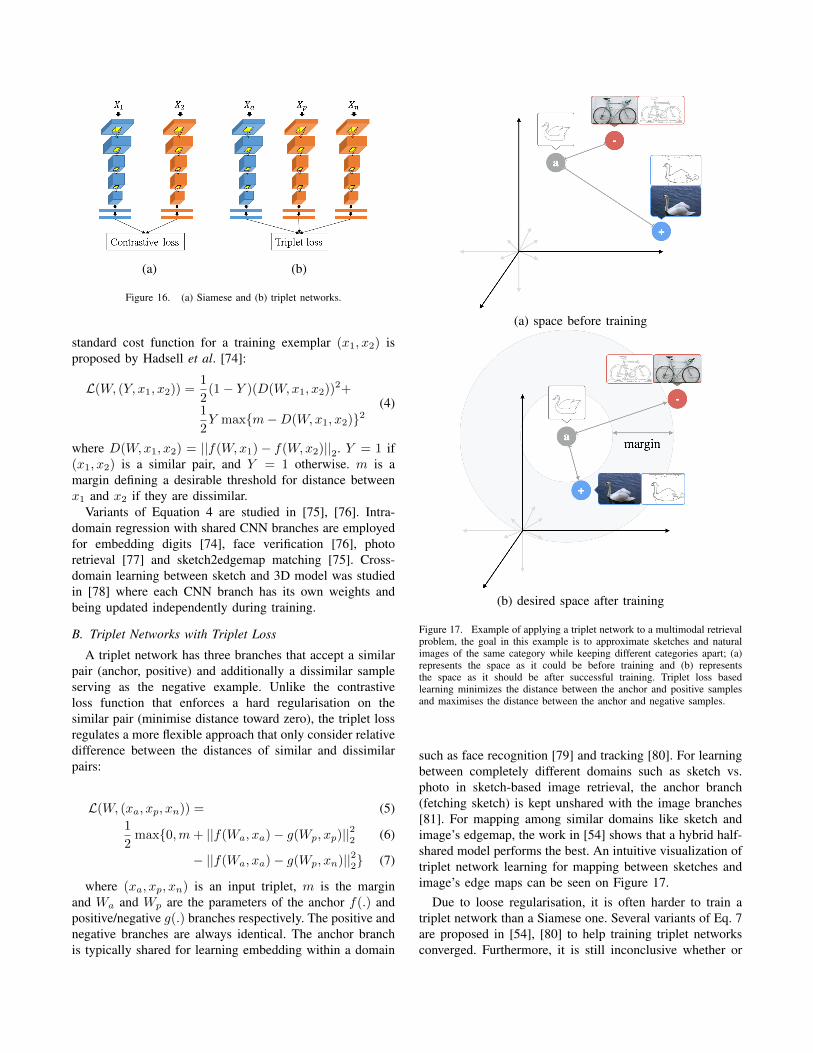
(a) (b)
Figure 16. (a) Siamese and (b) triplet networks.
standard cost function for a training exemplar (x1, x2) isproposed by Hadsell et al. [74]:
L(W, (Y, x1, x2)) =1
2(1− Y )(D(W,x1, x2))2+
1
2Y maxm−D(W,x1, x2)2
(4)
where D(W,x1, x2) = ||f(W,x1)− f(W,x2)||2. Y = 1 if(x1, x2) is a similar pair, and Y = 1 otherwise. m is amargin defining a desirable threshold for distance betweenx1 and x2 if they are dissimilar.
Variants of Equation 4 are studied in [75], [76]. Intra-domain regression with shared CNN branches are employedfor embedding digits [74], face verification [76], photoretrieval [77] and sketch2edgemap matching [75]. Cross-domain learning between sketch and 3D model was studiedin [78] where each CNN branch has its own weights andbeing updated independently during training.
B. Triplet Networks with Triplet Loss
A triplet network has three branches that accept a similarpair (anchor, positive) and additionally a dissimilar sampleserving as the negative example. Unlike the contrastiveloss function that enforces a hard regularisation on thesimilar pair (minimise distance toward zero), the triplet lossregulates a more flexible approach that only consider relativedifference between the distances of similar and dissimilarpairs:
L(W, (xa, xp, xn)) = (5)1
2max0,m+ ||f(Wa, xa)− g(Wp, xp)||22 (6)
− ||f(Wa, xa)− g(Wp, xn)||22 (7)
where (xa, xp, xn) is an input triplet, m is the marginand Wa and Wp are the parameters of the anchor f(.) andpositive/negative g(.) branches respectively. The positive andnegative branches are always identical. The anchor branchis typically shared for learning embedding within a domain
(a) space before training
(b) desired space after training
Figure 17. Example of applying a triplet network to a multimodal retrievalproblem, the goal in this example is to approximate sketches and naturalimages of the same category while keeping different categories apart; (a)represents the space as it could be before training and (b) representsthe space as it should be after successful training. Triplet loss basedlearning minimizes the distance between the anchor and positive samplesand maximises the distance between the anchor and negative samples.
such as face recognition [79] and tracking [80]. For learningbetween completely different domains such as sketch vs.photo in sketch-based image retrieval, the anchor branch(fetching sketch) is kept unshared with the image branches[81]. For mapping among similar domains like sketch andimage’s edgemap, the work in [54] shows that a hybrid half-shared model performs the best. An intuitive visualization oftriplet network learning for mapping between sketches andimage’s edge maps can be seen on Figure 17.
Due to loose regularisation, it is often harder to train atriplet network than a Siamese one. Several variants of Eq. 7are proposed in [54], [80] to help training triplet networksconverged. Furthermore, it is still inconclusive whether or

not triplet CNN is better than Siamese. Contrastive loss isseen to outperform triplet loss in [77], but marginally under-performs its counterpart in [54], [82]. Recently, there existstudies of another loss function that aims to overcome thedrawbacks of both contrastive and triplet losses, as claimedin the work of [83].
VII. APPLICATIONS
Here we describe Computer Vision and Image Process-ing applications that use the methods detailed in previoussections, by reviewing some of the recent literature on eachtopic.
A. Visual Stylization
Deep CNNs have also benefited visual content styliza-tion [84]. Echoing the transformation of visual recognitionpipelines from hand-engineered to end-to-end trained so-lutions, deep learning has delivered a step change in ourcapability to learn artistic styles by example, and to transferthat style to novel imagery - solving a major sub-problemwithin the Non-Photorealistic Rendering (NPR) field ofcomputer graphics [85].
Stylized output had already been explored in projectssuch as Google’s DeepDream [86], where backpropagationwas applied to optimize an input image toward an imagemaximising a one-hot output on a discriminative network(such as GoogLeNet). Initialising such a network with whitenoise converges the input toward an optimal trigger imagefor the desired object category. More interestingly, initial-ising the optimization from a photograph (plus Gaussianadditive i.e. white noise) will hallucinate a locally optimalimage in which structures resembling the one-hot object aretransformed to more closely represent that object.
Gatys et al. [87] went further, observing that such noisyimages could optimized to meet a dual objective – seekinga particular content (scene structure and composition) witha particular style (the appearance properties). Specifically,their ‘Neural Styles’ technique [87] accepted a pair ofimages (a photograph and an artwork) as input, and soughtto hallucinate an input image that matched the content ofthe input photograph, but matched the style of the inputartwork. A simplified structure of the techinque is presentedon Figure 18. The input image was again initialised from thephotograph plus white noise, and in their work a pre-traineddiscriminative network (VGG19, trained over ImageNet)was used for the optimization. During optimization networkweights are fixed, but the image is converged to minimiseloss LNS:
LNS(x; p, a) = αLcontent(p, x) + βLstyle(a, x)
where x refers the image being optimized, p refers tothe photograph and a refers to the example style image.Weights α = 1, β = 100 are typically chosen to balancethe two losses, which otherwise exhibit differing orders of
magnitude. The content loss compares features extractedfrom a late (semantic) layer of the VGG19 network —ideally these should match between p and x. The originalformulation uses the conv4 2 layer of VGG19 (assume F (.)extracts this image feature):
Lcontent =1
2
∑i,j
|F (p)− F (x)|2
The style loss is computed using several Gram (inner-product) matrices, each computed from the feature responsefrom a layer in VGG19. For a given layer l the gram matrixGl can be computed as an inner product of the vectorisedfeature map i and j within that layer (F li,j):
Gli,j(x) =∑k
F li,k(x)F lj,k(x).
The style loss simply sums(Gl(x)−Gl(a)
)2for several
layers l. In some implementations the sum is weighted toafford prominence to certain layers, but this has little prac-tical outcome. The style loss is commonly aggregated overa set of VGG19 layers conv1 1, conv2 1, . . . , conv5 1.
The use of the Gram matrix to encode style similarity wasthe core insight in this work, and fundamentally underpinsall subsequent work on deep learning for stylization. Forexample, recent work seeking to stylize video notes thatinstability in the Gram matrix over time is directly correlatedwith temporal incoherence (flicker) and seeks to minimizethat explicitly in the optimization [88].
Whilst optimization of the input image in this manneryields impressive aesthetics, the technique is slow. Morerecently, feed-forward networks have been used to stylizeimages in the order of seconds rather than minutes [89].Although current feed-forward designs somewhat degradestyle fidelity, their interactive speed has enabled video styl-ization and a slew of commercial (mobile app) software (e.g.Prisma, deepart.io) in the social media space. A discussionof feed-forward architectures for visual stylization is beyondthe scope of this tutorial, but we note that contemporaryarchitectures for video stylization integrate two stream net-works (again, pre-trained) – one branch dealing with image,the other optical flow, with the latter integrated into the lossfunction to minimise flicker [88], [90].
B. Image processing (pixels-to-pixels predictions)
Deep Networks for computer vision as seen so far are usu-ally designed for image classification and feature learning.In order to adapt such models to output images (instead ofclass labels or feature vectors), one must train the networkspixels-to-pixels. This kind of architecture is often calledFully convolutional or Image Processing Deep Networks,from which is possible to obtain for example semanticsegmentation [91]–[93], depth estimation [94], [95] andoptical flow [96].
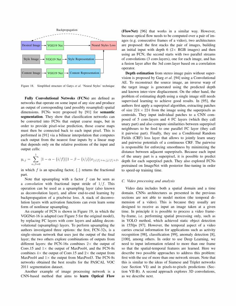
Desired Image VGG19 Net Neural Styles Loss
Style Image VGG19 Net Style Representation
Content Image VGG19 Net Content Representation
Backpropagation
Figure 18. Simplified structure of Gatys et al. ‘Neural Styles’ technique
Fully Convolutional Netwoks (FCNs) are defined asnetworks that operate on some input of any size and producean output of corresponding (and possibly resampled) spatialdimensions. FCNs were proposed by [91] for semanticsegmentation. They show that classification networks canbe converted into FCNs that output coarse maps, but inorder to provide pixel-wise prediction, those coarse mapsmust then be connected back to each input pixel. This isperformed in [91] via a bilinear interpolation that computeseach output from the nearest four inputs by a linear mapthat depends only on the relative positions of the input andoutput cells:
yi,j =
1∑α,β=0
|1− α− i/f||1− β − i/j|xbi/fc+α,bj/fc+β ,
in which f is an upscaling factor, . returns the fractionalpart.
Note that upsampling with a factor f can be seen asa convolution with fractional input stride of 1/f . Thisoperation can be used as a upsampling layer (also knownas deconvolution layer), and allow end-to-end learning bybackpropagation of a pixelwise loss. A stack of deconvo-lution layers with activation functions can even learn someform of nonlinear upsampling.
An example of FCN is shown in Figure 19, in which theVGGNet-16 is adapted (see Figure 5 for the original model),by replacing FC layers with conv layers and adding decon-volutional (upsampling) layers. To perform upsampling theauthors investigated three options: the first, FCN-32s, is asingle-stream network that uses just the output of the finallayer; the two others explore combinations of outputs fromdifferent layers: the FCN-16s combines 2× the output ofConv.15 and 1× the output of MaxPool4, and the FCN-8scombines 4× the output of Conv.15 and 2× the output fromMaxPool4 and 1× the output from MaxPool3. The FCN-8snetworks obtained the best results for the PASCAL VOC2011 segmentation dataset.
Another example of image processing network is aCNN-based method that aims to learn Optical Flow
(FlowNet) [96] that works in a similar way. However,because optical flow needs to be computed over a pair of im-ages (e.g. consecutive frames of a video), two architecturesare proposed: the first stacks the pair of images, buildingan initial input with depth 6 (2× RGB images) and thenusing an FCN; the second starts with two parallel streamsof convolutions (3 conv.layers), one for each image, and hasa fusion layer after the 3rd conv.layer based on a correlationoperator.
Depth estimation from stereo image pairs without super-vision is proposed by Garg et al. [94] using a ConvolutionalAE. To reconstruct the source image, an inverse warp ofthe target image is generated using the predicted depthand known inter-view displacement. On the other hand, theproblem of estimating depth using a single image still needssupervised learning to achieve good results. In [95], theauthors first apply a superpixel algorithm, extracting patchesof size 224 × 224 from the image using the superpixels ascentroids. They input individual patches to a CNN com-posed of 5 conv.layers and 4 FC layers (which they callunary part) and also compute similarities between superpixelneighbours to be feed to one parallel FC layer (they callit pairwise part). Finally, they use a Conditional RandomFields (CRF) loss layer that allows to jointly learn unaryand pairwise potentials of a continuous CRF. The pairwiseis responsible for enforcing smoothness by minimizing thedistance between adjacent superpixels. Because each inputof the unary part is a superpixel, it is possible to predictdepth for each superpixel patch. They also explored FCNspretrained on ImageNet with posterior fine-tuning in orderto speed-up training time.
C. Video processing and analysis
Video data includes both a spatial domain and a timedomain. CNNs architectures as presented in the previoussections are not able to model motion (the temporal di-mension of a video). This is because they usually aredesigned to receive as input an image taken at a giventime. In principle it is possible to process a video frame-by-frame, i.e. performing spatial processing only, such asin YOLO method, which achieved static object detectionin 155fps [97]. However, the temporal aspect of a videocarries crucial information for applications such as activityrecognition [98], classification [99], anomaly detection [8],[100], among others. In order to use Deep Learning, weneed to input information related to more than one frameso that the spatial-temporal features are learned. Here wedescribe two possible approaches to address this problem:first with the use of more than one network stream. Note thatthis is similar to the ideas of Siamese and Triplet networks(see Section VI) and in pixels-to-pixels predictions (Sec-tion VII-B). A second approach explores 3D convolutions,as we describe next.

Inpu
tim
age
...
Max
pool
ing
3
Con
v8
Con
v9
Con
v10
Max
pool
ing
4
Con
v11
Con
v12
Con
v13
Max
pool
ing
5
Con
v14
Con
v15
FCN
-32s
:32×
upsa
mpl
ing
FCN
-16s
:16×
upsa
mpl
ing
FCN
-8s:
8×up
sam
plin
g
Figure 19. A FCN based on the VGGNet-16 architecture (the layersbetween input and Max Pooling 3 are omitted). The FC layers 14 and15 are replaced by convolutional layers. There are 3 versions of de-convolutional/upsampling layers: (FCN-32s) upsample of 32× using theoutput of Conv15; (FCN-16s) upsample of 16× combining the outputs ofConv15 layer and MaxPool4 layer at stride 16; (FCN-8s) upsample of 8×combining the Conv15 and MaxPool4 layers with an additional MaxPool3output at stride 8.
– Multi-stream networks: deep networks for video useseveral streams of layers often using images and optical-flow to process video data. The Two-stream Network wasproposed by [98] and also used in [99]. In this framework,two CNN streams are employed; the first CNN (spatialstream) takes as input frames ft; the second CNN (temporalstream) takes as input the Optical Flow computed from pairsof L frames. Since each Optical Flow results in a verticaland a horizontal component, the input of the temporal streamCNN is composed of 2L input channels. In [98] they reportL = 10 as giving the best results. Each stream has its ownsoftmax classifier and respective loss function. A fusionof the two class scores is performed (using the sum) toobtain the overall training loss, from which an additionalloss function layer is used to compute the backpropagation.In [99], the authors use the Two-Stream network with anLSTM on the top in order to store information over timeand explore long-range dynamics.
In the context of anomaly detection, in which we onlyhave examples from the normal class, a three-stream au-toencoder was proposed using frames and optical-flow mapsto extract appearance, motion and joint representations [8].Those representations are then used to train a One ClassSVM classifier that is used to detect anomalies in videodata.
– Convolutional 3D: is a convolutional network thatconsiders sequences of frames as input in order to be usedfor videos. To do so, in [101] the authors propose to use3D convolutions and 3D pooling layers to create networksthat can jointly model the spatial and temporal dimensions
of a video. To prove the effectiveness of such approach theydeveloped an architecture, named Convolutional 3D (C3D)network.
Similarly to the VGG networks, C3D uses small convo-lutional kernels (3×3×3) to reduce the number of weightsto be learned, and 3D pooling layers with sizes 1 × 2 × 2(Pooling 1), and 2×2×2 (Pooling 2–5). The network takesas input 224× 224× 16 pixels (16 sequential frames, eachone with a 224×224 resolution). Note that applying a small3D convolution in a video volume results in another volumeas feature map, which preserves the temporal information tobe processed by further layers.
From an architectural point of view, C3D has 8 3D-convolutional, 2 FC, 5 max pooling and one softmax layers.Lastly, it applies a 0.5 dropout on FC6 and FC7. As theauthors show, the CD3 learns representations that capturethe appearance of the first frames, and thereafter showsactivation patterns referring to salient motion. Although theCD3 is able to take as input only fragments of videoscontaining 16 frames, the method obtained stated-of-the-artresults for action recognition in some challenging datasets(e.g. Sports-1M [102] and UCF101 [103])
VIII. LIMITATIONS OF DEEP LEARNING
Deep learning models for computer vision achieved statis-tically impressive results. As we show throughout this paper,the idea of stacking layers of operators that are trained tolearn hierarchical representations is useful to many applica-tions and contexts. By using different simple architecturessuch as CNNs, AEs or GANs, and their combination intomore complex architectures such as Siamese, Triplet, Multi-stream, etc., it is possible to implement strategies to solve avast number of applications.
There are, however, clear limitations with this kind ofapproach. Recall that neural networks (including deep net-works) are basically a way to learn a series of transforma-tions applied to an input vector so that it minimizes the lossfunction. In the case of classification, for example, the net-work learns how to transform input examples from differentclasses so that they are mapped to different regions of theoutput space, one example at a time. This transformationis given by a large set of weights (parameters) that areupdated during training stage so that the loss function isminimized. In order to allow training, the transformationmust be differentiable, i.e. the map between input and outputmust be continuous and ideally smooth, which presents asignificant constraint [21].
Whilst deep networks need very large annotated datasets,human beings are able to learn a concept by abstractionseeing just a few examples. To train a network to classifynumeric digits, we need hundreds or thousands of such digitsdrawn by different people, while humans usually are able tolearn the same concepts with a few examples drawn by oneperson only. We also easily adapt those concepts over time.

Figure 20. Adversarial examples visually unrecognizable, but classifiedwith more than 99% confidence by Deep Learning methods, as in [104].
Figure 21. Adversarial image generated by adding a cheetah gradientfeature to a picture of an owl, that is then classified with high confidenceas a cheetah by a state-of-the-art Deep Network.
Although generative models are a step towards this direction,since they represent an attempt to model the distribution thatgenerates the data categories, those are still a long way fromthe human learning capacity.
Even considering tasks that are in principle possible tobe addressed via Deep Learning, there are many studiesshowing that perturbations in the input data, such as noise,can significantly impact the results [44]. An interesting papershowed that deep networks can even fail to classify invertedimages [105]. It is possible to create images that appear tobe just random noise and are unrecognizable to humans,but that CNNs believe to belong to some known class withmore than 99% of certainty [104] as examples shown inFigure 20. Based on those unrecognizable patterns, it ispossible to design small perturbations (around 4%) addedto images so that the output of such methods is completelywrong [106]. In Figure 21 we adapt a famous example byadding a cheetah gradient feature to an owl image so thatit is imperceptible to humans, but that is then classifiedwith high confidence as cheetah by a Deep Network. Inorder to alleviate such fragility to attacks, recent studiesrecommend to add adversarial examples to the trainingset or to increase the capacity (in terms of number offilters/nodes per layer), increasing the number of parametersand therefore the complexity of space of functions allowed inthe model [107], [108]. Therefore, although the performanceof such methods can be impressive when considering overallresults, the outputs can be individually unreliable.
If we analyze those already mentioned scenarios in thepoint of view of Statistical Learning Theory [109], wecould hypothesize that those methods are in fact learningthe memory-based model. They work well in several cases
because they are trained with up to millions of examples,thus unseen data that is similar to training data will even-tually fall inside the memorized regions. Although recentwork including tensor analysis of representations [110] anduncertainty [111] tried to shed light on learning behaviourof deep networks, more studies on theoretical aspects relatedto Deep Learning are still needed.
Nevertheless, the positive impact of Deep Learning inComputer Vision and Image Processing is undeniable. Byunderstanding its limitations and inner workings, researcherscan explore those methods for many years to come andcontinue to develop exciting results for new applications.
ACKNOWLEDGMENT
The authors would like to thank FAPESP (grants #2016-16411-4, #2017/10068-2, #2015/04883-0, #2013/07375-0)and the Santander Mobility Award.
REFERENCES
[1] J. Deng, W. Dong, R. Socher, L.-J. Li, K. Li, and L. Fei-Fei,“ImageNet: A Large-Scale Hierarchical Image Database,” inCVPR09, 2009.
[2] O. Russakovsky, J. Deng, H. Su, J. Krause, S. Satheesh,S. Ma, Z. Huang, A. Karpathy, A. Khosla, M. Bernstein,A. C. Berg, and L. Fei-Fei, “ImageNet Large Scale VisualRecognition Challenge,” International Journal of ComputerVision (IJCV), vol. 115, no. 3, pp. 211–252, 2015.
[3] K. Fukushima, “Neocognitron: A hierarchical neural net-work capable of visual pattern recognition,” Neural net-works, vol. 1, no. 2, pp. 119–130, 1988.
[4] Y. LeCun, L. Bottou, Y. Bengio, and P. Haffner, “Gradient-based learning applied to document recognition,” Proceed-ings of the IEEE, vol. 86, no. 11, pp. 2278–2324, 1998.
[5] S. Lazebnik, C. Schmid, and J. Ponce, “Beyond bags offeatures: Spatial pyramid matching for recognizing naturalscene categories,” in Computer Vision and Pattern Recogni-tion, 2006 IEEE Conf. on, vol. 2. IEEE, 2006, pp. 2169–2178.
[6] A. Krizhevsky, I. Sutskever, and G. E. Hinton, “Imagenetclassification with deep convolutional neural networks,” inAdvances in Neural Information Processing Systems 25:26th Annual Conference on Neural Information ProcessingSystems., 2012, pp. 1106–1114.
[7] L. Zhang, L. Zhang, and B. Du, “Deep learning for remotesensing data: A technical tutorial on the state of the art,”IEEE Geoscience and Remote Sensing Magazine, vol. 4,no. 2, pp. 22–40, 2016.
[8] D. Xu, E. Ricci, Y. Yan, J. Song, and N. Sebe, “Learningdeep representations of appearance and motion for anoma-lous event detection.” in British Matchine Vision Conference(BMVC), X. Xie, M. W. Jones, and G. K. L. Tam, Eds.BMVA Press, 2015.
[9] M. Ravanbakhsh, M. Nabi, H. Mousavi, E. Sangineto,and N. Sebe, “Plug-and-play CNN for crowd motionanalysis: An application in abnormal event detection,”CoRR, vol. abs/1610.00307, 2016. [Online]. Available:http://arxiv.org/abs/1610.00307
[10] I. B. Barbosa, M. Cristani, B. Caputo, A. Rognhaugen, andT. Theoharis, “Looking beyond appearances: Synthetic train-ing data for deep cnns in re-identification,” arXiv preprintarXiv:1701.03153, 2017.
[11] A. Fischer and C. Igel, “Training restricted boltzmann ma-chines: An introduction,” Pattern Recognition, vol. 47, no. 1,pp. 25–39, 2014.
[12] H. Larochelle, M. Mandel, R. Pascanu, and Y. Bengio,“Learning algorithms for the classification restricted boltz-mann machine,” Journal of Machine Learning Research,vol. 13, no. Mar, pp. 643–669, 2012.
[13] R. Salakhutdinov and G. Hinton, “Deep boltzmann ma-chines,” in Artificial Intelligence and Statistics, 2009, pp.448–455.
[14] G. E. Hinton, S. Osindero, and Y.-W. Teh, “A fast learningalgorithm for deep belief nets,” Neural computation, vol. 18,no. 7, pp. 1527–1554, 2006.
[15] S. Zheng, S. Jayasumana, B. Romera-Paredes, V. Vineet,Z. Su, D. Du, C. Huang, and P. Torr, “Conditional randomfields as recurrent neural networks,” in International Con-ference on Computer Vision (ICCV), 2015.
[16] A. Graves, A.-r. Mohamed, and G. Hinton, “Speech recog-nition with deep recurrent neural networks,” in IEEE In-ternational Conference on Acoustics, Speech and SignalProcessing (ICASSP), 2013, pp. 6645–6649.
[17] R. Pascanu, T. Mikolov, and Y. Bengio, “On the difficultyof training recurrent neural networks,” in International Con-ference on Machine Learning, 2013, pp. 1310–1318.
[18] R. Gonzalez and R. Woods, Digital Image Processing,3rd ed. Pearson, 2007.
[19] S. Ben-David and S. Shalev-Shwartz, Understanding Ma-chine Learning: from theory to algorithms. Cambridge,2014.
[20] I. Goodfellow, Y. Bengio, and A. Courville, Deep Learning.MIT Press, 2016, http://www.deeplearningbook.org.
[21] F. Chollet, Deep Learning with Python. Manning, 2017.
[22] K. Simonyan and A. Zisserman, “Very deep convolutionalnetworks for large-scale image recognition,” CoRR, vol.abs/1409.1556, 2014.
[23] K. He, X. Zhang, S. Ren, and J. Sun, “Deep residual learningfor image recognition,” CoRR, vol. abs/1512.03385, 2015.
[24] C. Szegedy, V. Vanhoucke, S. Ioffe, J. Shlens, and Z. Wojna,“Rethinking the inception architecture for computer vision,”CoRR, vol. abs/1512.00567, 2015.
[25] G. Huang, Z. Liu, L. van der Maaten, and K. Q. Weinberger,“Densely connected convolutional networks,” in Proceedingsof the IEEE Conference on Computer Vision and PatternRecognition, 2017.
[26] V. Nair and G. E. Hinton, “Rectified linear units improverestricted boltzmann machines,” in Proceedings of the 27thInternational Conference on Machine Learning (ICML-10),J. Furnkranz and T. Joachims, Eds. Omnipress, 2010, pp.807–814.
[27] K. He, X. Zhang, S. Ren, and J. Sun, Identity Mappingsin Deep Residual Networks. Cham: Springer InternationalPublishing, 2016, pp. 630–645. [Online]. Available: https://doi.org/10.1007/978-3-319-46493-0 38
[28] M. Ponti, E. S. Helou, P. J. S. Ferreira, and N. D. Mas-carenhas, “Image restoration using gradient iteration andconstraints for band extrapolation,” IEEE Journal of SelectedTopics in Signal Processing, vol. 10, no. 1, pp. 71–80, 2016.
[29] K. He, X. Zhang, S. Ren, and J. Sun, “Delving deep intorectifiers: Surpassing human-level performance on imagenetclassification,” in Proceedings of the IEEE internationalconference on computer vision, 2015, pp. 1026–1034.
[30] J. T. Springenberg, A. Dosovitskiy, T. Brox, andM. Riedmiller, “Striving for simplicity: The allconvolutional net,” in ICLR (workshop track), 2015.[Online]. Available: http://lmb.informatik.uni-freiburg.de/Publications/2015/DB15a
[31] Y. A. LeCun, L. Bottou, G. B. Orr, and K.-R. Muller,“Efficient backprop,” in Neural networks: Tricks of the trade.Springer, 2012, pp. 9–48.
[32] S. Ioffe and C. Szegedy, “Batch normalization: Acceleratingdeep network training by reducing internal covariate shift,”in International Conference on Machine Learning, 2015, pp.448–456.
[33] M. Ponti, J. Kittler, M. Riva, T. de Campos, and C. Zor, “Adecision cognizant Kullback–Leibler divergence,” PatternRecognition, vol. 61, pp. 470–478, 2017.
[34] J. Duchi, E. Hazan, and Y. Singer, “Adaptive subgradientmethods for online learning and stochastic optimization,”Journal of Machine Learning Research, vol. 12, no. Jul, pp.2121–2159, 2011.
[35] M. D. Zeiler, “Adadelta: an adaptive learning rate method,”arXiv preprint arXiv:1212.5701, 2012.
[36] D. Kingma and J. Ba, “Adam: A method for stochasticoptimization,” in 3rd International Conference on LearningRepresentations (ICLR), 2015.
[37] M. Li, T. Zhang, Y. Chen, and A. J. Smola, “Efficient mini-batch training for stochastic optimization,” in Proceedingsof the 20th ACM SIGKDD international conference onKnowledge discovery and data mining. ACM, 2014, pp.661–670.
[38] L. Bottou, F. E. Curtis, and J. Nocedal, “Optimizationmethods for large-scale machine learning,” arXiv preprintarXiv:1606.04838, 2016.

[39] P. Goyal, P. Dollar, R. Girshick, P. Noordhuis,L. Wesolowski, A. Kyrola, A. Tulloch, Y. Jia,and K. He, “Accurate, large minibatch SGD:Training imagenet in 1 hour.” [Online]. Available:https://research.fb.com/publications/imagenet1kin1h/
[40] G. E. Hinton, N. Srivastava, A. Krizhevsky, I. Sutskever,and R. R. Salakhutdinov, “Improving neural networks bypreventing co-adaptation of feature detectors,” arXiv preprintarXiv:1207.0580, 2012.
[41] D. Warde-Farley, I. J. Goodfellow, A. Courville, andY. Bengio, “An empirical analysis of dropout in piecewiselinear networks,” in ICLR 2014, 2014. [Online]. Available:arXivpreprintarXiv:1312.6197
[42] C. Szegedy, V. Vanhoucke, S. Ioffe, J. Shlens, and Z. Wojna,“Rethinking the inception architecture for computer vision,”in Proceedings of the IEEE Conference on Computer Visionand Pattern Recognition, 2016, pp. 2818–2826.
[43] K. Chatfield, K. Simonyan, A. Vedaldi, and A. Zisserman,“Return of the devil in the details: Delving deep intoconvolutional nets,” in British Machine Vision Conference(BMVC), 2014, p. 1405.3531.
[44] T. Nazare, G. Paranhos da Costa, W. Contato, and M. Ponti,“Deep convolutional neural networks and noisy images,” inIberoamerican Conference on Pattern Recognition (CIARP),2017.
[45] C. Szegedy, S. Ioffe, V. Vanhoucke, and A. A. Alemi,“Inception-v4, inception-resnet and the impact of residualconnections on learning.” in AAAI, 2017, pp. 4278–4284.
[46] F. N. Iandola, S. Han, M. W. Moskewicz, K. Ashraf, W. J.Dally, and K. Keutzer, “Squeezenet: Alexnet-level accuracywith 50x fewer parameters and¡ 0.5 mb model size,” inICLR, 2016.
[47] H.-C. Shin, H. R. Roth, M. Gao, L. Lu, Z. Xu, I. Nogues,J. Yao, D. Mollura, and R. M. Summers, “Deep convolu-tional neural networks for computer-aided detection: Cnnarchitectures, dataset characteristics and transfer learning,”IEEE transactions on medical imaging, vol. 35, no. 5, pp.1285–1298, 2016.
[48] A. S. Razavian, H. Azizpour, J. Sullivan, and S. Carlsson,“Cnn features off-the-shelf: An astounding baseline forrecognition,” in Proceedings of the 2014 IEEE Conferenceon Computer Vision and Pattern Recognition Workshops,ser. CVPRW ’14. Washington, DC, USA: IEEE ComputerSociety, 2014, pp. 512–519.
[49] M. Oquab, L. Bottou, I. Laptev, and J. Sivic, “Learningand transferring mid-level image representations using con-volutional neural networks,” in Proceedings of the IEEEconference on computer vision and pattern recognition,2014, pp. 1717–1724.
[50] S. M. Erfani, S. Rajasegarar, S. Karunasekera, and C. Leckie,“High-dimensional and large-scale anomaly detection usinga linear one-class svm with deep learning,” Pattern Recog-nition, vol. 58, pp. 121–134, 2016.
[51] M. Ponti, T. S. Nazare, and G. S. Thume, “Image quanti-zation as a dimensionality reduction procedure in color andtexture feature extraction,” Neurocomputing, vol. 173, pp.385–396, 2016.
[52] Y. Kalantidis and Y. Avrithis, “Locally optimized productquantization for approximate nearest neighbor search,” inProceedings of the IEEE Conference on Computer Visionand Pattern Recognition, 2014, pp. 2321–2328.
[53] T. Bui, L. Ribeiro, M. Ponti, and J. Collomosse, “Compactdescriptors for sketch-based image retrieval using a tripletloss convolutional neural network,” Computer Vision andImage Understanding, 2017.
[54] ——, “Generalisation and sharing in triplet convnetsfor sketch based visual search,” arXiv preprintarXiv:1611.05301, 2016.
[55] Y. Bengio, A. Courville, and P. Vincent, “Representationlearning: A review and new perspectives,” IEEE Trans.Pattern Anal. Mach. Intell., vol. 35, no. 8, pp. 1798–1828,Aug. 2013.
[56] J. Masci, U. Meier, D. Ciresan, and J. Schmidhuber,“Stacked convolutional auto-encoders for hierarchical fea-ture extraction,” Artificial Neural Networks and MachineLearning–ICANN 2011, pp. 52–59, 2011.
[57] P. Vincent, H. Larochelle, I. Lajoie, Y. Bengio, and P.-A.Manzagol, “Stacked denoising autoencoders: Learning use-ful representations in a deep network with a local denoisingcriterion,” Journal of Machine Learning Research, vol. 11,no. Dec, pp. 3371–3408, 2010.
[58] G. Alain and Y. Bengio, “What regularized auto-encoderslearn from the data-generating distribution,” The Journal ofMachine Learning Research, vol. 15, no. 1, pp. 3563–3593,2014.
[59] S. Rifai, G. Mesnil, P. Vincent, X. Muller, Y. Bengio,Y. Dauphin, and X. Glorot, “Higher order contractive auto-encoder,” Machine Learning and Knowledge Discovery inDatabases, pp. 645–660, 2011.
[60] B. Scholkopf, A. Smola, and K.-R. Muller, “Nonlinearcomponent analysis as a kernel eigenvalue problem,” Neuralcomputation, vol. 10, no. 5, pp. 1299–1319, 1998.
[61] Y. Bengio, L. Yao, G. Alain, and P. Vincent, “Generalizeddenoising auto-encoders as generative models,” in Advancesin Neural Information Processing Systems, 2013, pp. 899–907.
[62] C. Doersch, “Tutorial on variational autoencoders,” arXivpreprint arXiv:1606.05908, 2016.
[63] D. J. Rezende, S. Mohamed, and D. Wierstra,“Stochastic backpropagation and approximate inferencein deep generative models,” in Proceedings of the31st International Conference on Machine Learning, ser.Proceedings of Machine Learning Research, E. P. Xing andT. Jebara, Eds., vol. 32, no. 2. Bejing, China: PMLR,22–24 Jun 2014, pp. 1278–1286. [Online]. Available:http://proceedings.mlr.press/v32/rezende14.html
[64] D. P. Kingma, “Fast Gradient-Based Inference withContinuous Latent Variable Models in Auxiliary Form,” jun2013. [Online]. Available: http://arxiv.org/abs/1306.0733
[65] I. J. Goodfellow, J. Pouget-Abadie, M. Mirza, B. Xu,D. Warde-Farley, S. Ozair, A. Courville, and Y. Bengio,“Generative adversarial nets,” in Advances in Neural Infor-mation Processing Systems 27, 2014.
[66] B. J. Frey, G. E. Hinton, and P. Dayan, “Does the wake-sleepalgorithm produce good density estimators?” in Advances inNeural Information Processing Systems 8, D. S. Touretzky,M. C. Mozer, and M. E. Hasselmo, Eds. MIT Press, 1996,pp. 661–667.
[67] B. J. Frey, Graphical models for machine learningand digital communication. MIT Press, 1998.[Online]. Available: https://mitpress.mit.edu/books/graphical-models-machine-learning-and-digital-communication
[68] A. van den Oord, S. Dieleman, H. Zen, K. Simonyan,O. Vinyals, A. Graves, N. Kalchbrenner, A. Senior,and K. Kavukcuoglu, “WaveNet: A Generative Modelfor Raw Audio,” sep 2016. [Online]. Available: http://arxiv.org/abs/1609.03499
[69] S. E. Fahlman, G. E. Hinton, and T. J. Sejnowski,“Massively parallel architectures for ai: Netl, thistle,and boltzmann machines,” in Proceedings of the ThirdAAAI Conference on Artificial Intelligence, ser. AAAI’83.AAAI Press, 1983, pp. 109–113. [Online]. Available:http://dl.acm.org/citation.cfm?id=2886844.2886868
[70] G. E. Hinton, “Learning multiple layers of representation,”pp. 428–434, 2007. [Online]. Available: http://www.cs.toronto.edu/∼fritz/absps/tics.pdf
[71] J.-Y. Zhu, T. Park, P. Isola, and A. A. Efros, “Unpairedimage-to-image translation using cycle-consistent adver-sarial networks,” in ICLR 2017, 2017, p. arXiv preprintarXiv:1703.10593.
[72] P. Isola, J.-Y. Zhu, T. Zhou, and A. A. Efros, “Image-to-image translation with conditional adversarial networks,” inCVPR 2017, 2017, p. arXiv preprint arXiv:1611.07004.
[73] I. Goodfellow, “NIPS 2016 Tutorial: Generative AdversarialNetworks,” dec 2016. [Online]. Available: http://arxiv.org/abs/1701.00160
[74] R. Hadsell, S. Chopra, and Y. LeCun, “Dimensionalityreduction by learning an invariant mapping,” in Computervision and pattern recognition, 2006 IEEE computer societyconference on, vol. 2. IEEE, 2006, pp. 1735–1742.
[75] Y. Qi, Y.-Z. Song, H. Zhang, and J. Liu, “Sketch-basedimage retrieval via siamese convolutional neural network,”in Image Processing (ICIP), 2016 IEEE International Con-ference on. IEEE, 2016, pp. 2460–2464.
[76] S. Chopra, R. Hadsell, and Y. LeCun, “Learning a similaritymetric discriminatively, with application to face verifica-tion,” in Computer Vision and Pattern Recognition, 2005.CVPR 2005. IEEE Computer Society Conference on, vol. 1.IEEE, 2005, pp. 539–546.
[77] F. Radenovic, G. Tolias, and O. Chum, “Cnn image re-trieval learns from bow: Unsupervised fine-tuning with hardexamples,” in European Conference on Computer Vision.Springer, 2016, pp. 3–20.
[78] F. Wang, L. Kang, and Y. Li, “Sketch-based 3d shape re-trieval using convolutional neural networks,” in Proceedingsof the IEEE Conference on Computer Vision and PatternRecognition, 2015, pp. 1875–1883.
[79] F. Schroff, D. Kalenichenko, and J. Philbin, “Facenet: Aunified embedding for face recognition and clustering,” inProceedings of the IEEE Conference on Computer Visionand Pattern Recognition, 2015, pp. 815–823.
[80] X. Wang and A. Gupta, “Unsupervised learning of visualrepresentations using videos,” in Proceedings of the IEEEInternational Conference on Computer Vision, 2015, pp.2794–2802.
[81] P. Sangkloy, N. Burnell, C. Ham, and J. Hays, “The sketchydatabase: learning to retrieve badly drawn bunnies,” ACMTransactions on Graphics (TOG), vol. 35, no. 4, p. 119,2016.
[82] E. Hoffer and N. Ailon, “Deep metric learning using tripletnetwork,” in International Workshop on Similarity-BasedPattern Recognition. Springer, 2015, pp. 84–92.
[83] O. Rippel, M. Paluri, P. Dollar, and L. D. Bourdev, “Metriclearning with adaptive density discrimination,” CoRR, vol.abs/1511.05939, 2015.
[84] P. Rosin and J. C. (Eds.), Image and Video based ArtisticStylization. Springer, 2013.
[85] J.-E. Kyprianidis, J. Collomosse, T. Wang, and T. Isenberg,“State of the ’art’: A taxonomy of artistic stylization tech-niques for images and video,” IEEE Trans. Visualization andComp. Graphics (TVCG), 2012.
[86] A. Mordvintsev, M. Tyka, and C. Olah, “Deepdream,” https://github.com/google/deepdream, 2015.
[87] L. Gatys, A. Ecker, and M. Bethge, “A neural algorithm ofartistic style,” arXiv preprint arXiv:1508.06576, 2015.
[88] D. Chen, J. Liao, L. Yuan, N. Yu, and G. Hua, “Coherentonline video style transfer,” in Proc. Intl. Conf. ComputerVision (ICCV), 2017.
[89] D. Ulyanov, V. Lebedev, A. Vedaldi, and V. Lempitsky,“Texture networks: Feed-forward synthesis of textures andstylized images,” in Proc. Intl. Conf. Machine Learning(ICML), 2016.
[90] A. Gupta, J. Johnson, A. Alahi, and L. Fei-Fei, “Stabilityin neural style transfer: Characterization and application,” inProc. Intl. Conf. Computer Vision (ICCV), 2017.
[91] E. Shelhamer, J. Long, and T. Darrell, “Fully convolutionalnetworks for semantic segmentation,” IEEE Transactions onPattern Analysis and Machine Intelligence, vol. 39, no. 4,pp. 640–651, 2017.

[92] V. Badrinarayanan, A. Kendall, and R. Cipolla, “Segnet: Adeep convolutional encoder-decoder architecture for scenesegmentation,” IEEE transactions on pattern analysis andmachine intelligence, 2017.
[93] L.-C. Chen, J. T. Barron, G. Papandreou, K. Murphy, andA. L. Yuille, “Semantic image segmentation with task-specific edge detection using cnns and a discriminativelytrained domain transform,” in Proceedings of the IEEEConference on Computer Vision and Pattern Recognition,2016, pp. 4545–4554.
[94] R. Garg, G. Carneiro, and I. Reid, “Unsupervised cnn forsingle view depth estimation: Geometry to the rescue,” inEuropean Conference on Computer Vision. Springer, 2016,pp. 740–756.
[95] F. Liu, C. Shen, G. Lin, and I. Reid, “Learning depth fromsingle monocular images using deep convolutional neuralfields,” IEEE Transactions on Pattern Analysis and MachineIntelligence, vol. 38, no. 10, pp. 2024–2039, 2016.
[96] A. Dosovitskiy, P. Fischer, E. Ilg, P. Hausser, C. Hazirbas,V. Golkov, P. van der Smagt, D. Cremers, and T. Brox,“Flownet: Learning optical flow with convolutional net-works,” in Proceedings of the IEEE International Confer-ence on Computer Vision, 2015, pp. 2758–2766.
[97] J. Redmon, S. Divvala, R. Girshick, and A. Farhadi, “Youonly look once: Unified, real-time object detection,” inProceedings of the IEEE Conference on Computer Visionand Pattern Recognition, 2016, pp. 779–788.
[98] K. Simonyan and A. Zisserman, “Two-stream convolutionalnetworks for action recognition in videos,” in Advances inneural information processing systems, 2014, pp. 568–576.
[99] Z. Wu, X. Wang, Y.-G. Jiang, H. Ye, and X. Xue, “Modelingspatial-temporal clues in a hybrid deep learning frameworkfor video classification,” in Proceedings of the 23rd ACMinternational conference on Multimedia. ACM, 2015, pp.461–470.
[100] M. Ponti, T. S. Nazare, and J. Kittler, “Optical-flow fea-tures empirical mode decomposition for motion anomalydetection,” in IEEE International Conference on Acoustics,Speech and Signal Processing (ICASSP). IEEE, 2017, pp.1403–1407.
[101] D. Tran, L. Bourdev, R. Fergus, L. Torresani, and M. Paluri,“Learning spatiotemporal features with 3d convolutionalnetworks,” in Proceedings of the IEEE International Con-ference on Computer Vision, 2015, pp. 4489–4497.
[102] A. Karpathy, G. Toderici, S. Shetty, T. Leung, R. Sukthankar,and L. Fei-Fei, “Large-scale video classification with con-volutional neural networks,” in CVPR, 2014.
[103] K. Soomro, A. R. Zamir, and M. Shah, “UCF101: A datasetof 101 human actions classes from videos in the wild,”CoRR, vol. abs/1212.0402, 2012.
[104] A. Nguyen, J. Yosinski, and J. Clune, “Deep neural networksare easily fooled: High confidence predictions for unrecog-nizable images,” in IEEE Conference on Computer Visionand Pattern Recognition (CVPR), 2015, pp. 427–436.
[105] H. Hosseini and R. Poovendran, “Deep neural net-works do not recognize negative images,” arXiv preprintarXiv:1703.06857, 2017.
[106] N. Papernot, P. McDaniel, S. Jha, M. Fredrikson, Z. B.Celik, and A. Swami, “The limitations of deep learningin adversarial settings,” in IEEE European Symposium onSecurity and Privacy (EuroS&P). IEEE, 2016, pp. 372–387.
[107] A. Rozsa, M. Gunther, and T. E. Boult, “Are accuracy androbustness correlated,” in Machine Learning and Applica-tions (ICMLA), 2016 15th IEEE International Conferenceon. IEEE, 2016, pp. 227–232.
[108] A. Madry, A. Makelov, L. Schmidt, D. Tsipras, andA. Vladu, “Towards deep learning models resistant to ad-versarial attacks,” arXiv preprint arXiv:1706.06083, 2017.
[109] V. Vapnik, The nature of statistical learning theory.Springer science & business media, 2013.
[110] N. Cohen, O. Sharir, and A. Shashua, “On the expressivepower of deep learning: A tensor analysis,” in Conferenceon Learning Theory, 2016, pp. 698–728.
[111] Y. Gal and Z. Ghahramani, “Dropout as a bayesian approx-imation: Representing model uncertainty in deep learning,”in International Conference on Machine Learning, 2016, pp.1050–1059.