Department of Physics, Chemistry and Biology

Master’s Thesis

Evaluation of the Carbonization of Thermo-Stabilized

Lignin Fibers into Carbon Fibers

Henrik Kleinhans

5th July 2015

LITH-IFM-A-EX--15/3112--SE

Linköping University Department of Physics, Chemistry and Biology

581 83 Linköping

Department of Physics, Chemistry and Biology

Evaluation of the Carbonization of Thermo-Stabilized

Lignin Fibers into Carbon Fibers

Henrik Kleinhans

Thesis work performed at INNVENTIA AB

5th July 2015

Supervisors

Professor Lennart Salmén, INNVENTIA AB

Daniel Aili, Linköping University

Examiner

Dr. Thomas Ederth, Linköping University

Linköping University Department of Physics, Chemistry and Biology

581 83 Linköping

Abstract

Thermo-stabilized lignin fibers from pH-fractionated softwood kraft lignin were carbonized to

various temperatures during thermomechanical analysis (TMA) under static and increasing

load and different rates of heating. The aim was to optimize the carbonization process to

obtain suitable carbon fiber material with good mechanical strength potential (high tensile

strength and high E-modulus). The carbon fibers were therefore mainly evaluated of

mechanical strength in Dia-Stron uniaxial tensile testing.

In addition, chemical composition, in terms of functional groups, and elemental (atomic)

composition was studied in Fourier transform infrared spectroscopy (FTIR) and in energy-

dispersive X-ray spectroscopy (EDS), respectively. The structure of carbon fibers was imaged

in scanning electron microscope (SEM) and light microscopy. Thermogravimetrical analysis

was performed on thermo-stabilized lignin fibers to evaluate the loss of mass and to calculate

the stress-changes and diameter-changes that occur during carbonization.

The TMA-analysis of the deformation showed, for thermo-stabilized lignin fibers, a

characteristic behavior of contraction during carbonization. Carbonization temperatures above

1000°C seemed most efficient in terms of E-modulus and tensile strength whereas rate of

heating did not matter considerably. The E-modulus for the fibers was improved significantly

by slowly increasing the load during the carbonization. The tensile strength remained however

unchanged.

The FTIR-analysis indicated that many functional groups, mainly oxygen containing,

dissociate from the lignin polymers during carbonization. The EDS supported this by showing

that the oxygen content decreased. Accordingly, the relative carbon content increased

passively to around 90% at 1000°C. Aromatic structures in the carbon fibers are thought to

contribute to the mechanical strength and are likely formed during the carbonization.

However, the FTIR result showed no evident signs that aromatic structures had been formed,

possible due to some difficulties with the KBr-method.

In the SEM and light microscopy imaging one could observe that porous formations on the

surface of the fibers increased as the temperature increased in the carbonization. These

formations may have affected the mechanical strength of the carbon fibers, mainly tensile

strength.

The carbonization process was optimized in the sense that any heating rate can be used. No

restriction in production speed exists. The carbonization should be run to at least 1000°C to

achieve maximum mechanical strength, both in E-modulus and tensile strength. To improve

the E-modulus further, a slowly increasing load can be applied to the lignin fibers during

carbonization. The earlier the force is applied, to counteract the lignin fiber contraction that

occurs (namely around 300°C), the better. However, in terms of mechanical performance, the

lignin carbon fibers are still far from practical use in the industry.

Abbreviations

DLaTGS Deuterated L-alanine doped Triglycene Sulphate

DSC Differential Scanning Calorimetry

EDS Energy Dispersive X-ray Spectrometer

E-modulus Elastic modulus, Young’s modulus

FTIR Fourier Transform Infrared Spectroscopy

G Guaiacyl

GC Gas chromatograph

H P-hydroxyphenyl (P=para)

IR Infrared

Mn Number Average Molecular Weight

MPP Mesophase pitch

Mw Average Molecular Weight

PAN Polyacrylonitrile

PDI Polydispersity Index

S Syringyl

SEM Scanning Electron Microscope

TE Thermo Electric

Tg Glass Transition Temperature

TGA Thermogravimetric Analysis

TMA Thermomechanical Analysis

Ts Softening Point

v Version

WD Working Distance

i

Contents

1 Introduction ......................................................................................................................... 1

1.1 Aim ............................................................................................................................. 1

1.2 Background ................................................................................................................ 1

1.2.1 Polymer properties ............................................................................................... 3

1.2.2 Carbon fibers ........................................................................................................ 4

1.2.2.1 PAN-based carbon fibers .............................................................................. 4

1.2.2.2 Pitch-based carbon fibers .............................................................................. 5

1.2.2.3 Structure of carbon fibers .............................................................................. 6

1.2.3 Lignin polymer ..................................................................................................... 7

1.2.3.1 Refining of lignin ........................................................................................ 10

1.2.3.2 Lignin-based carbon fibers.......................................................................... 10

1.2.3.3 Production of lignin carbon fiber ................................................................ 11

2 Experimental ..................................................................................................................... 15

2.1 Stabilization .............................................................................................................. 15

2.2 Carbonization and Thermomechanical Analysis (TMA) ......................................... 16

2.2.1 Principles ............................................................................................................ 16

2.2.2 Method ............................................................................................................... 17

2.3 Uniaxial Tensile Testing (with Dia-Stron) ............................................................... 20

2.3.1 Principles ............................................................................................................ 20

2.3.2 Method ............................................................................................................... 20

2.4 Thermogravimetric Analysis (TGA) ........................................................................ 22

2.4.1 Principles ............................................................................................................ 22

2.4.2 Method ............................................................................................................... 22

2.5 Fourier Transform Infrared Spectroscopy (FTIR) ................................................... 23

2.5.1 Principles ............................................................................................................ 24

2.5.2 Method ............................................................................................................... 25

2.6 Scanning Electron Microscope (SEM) ..................................................................... 27

2.6.1 Principles ............................................................................................................ 27

2.6.2 Method ............................................................................................................... 28

2.7 Light Microscopy ..................................................................................................... 29

3 Results ............................................................................................................................... 30

3.1 TMA ......................................................................................................................... 30

ii

3.1.1 Static measurement ............................................................................................ 30

3.1.2 Measurements with increasing force .................................................................. 35

3.2 Dia-stron ................................................................................................................... 39

3.2.1 Evaluation of temperature and heating rate ........................................................ 39

3.2.2 Evaluation of applied force during carbonization .............................................. 45

3.3 TGA .......................................................................................................................... 47

3.4 FTIR ......................................................................................................................... 52

3.5 SEM .......................................................................................................................... 60

3.5.1 Imaging ............................................................................................................... 60

3.5.2 Energy-dispersive X-ray spectroscopy ............................................................... 64

3.6 Light Microscopy ..................................................................................................... 69

4 Discussion ......................................................................................................................... 74

4.1 Analysis of the main results ..................................................................................... 74

4.1.1 TMA ................................................................................................................... 74

4.1.2 Dia-Stron ............................................................................................................ 74

4.1.3 TGA .................................................................................................................... 76

4.1.4 FTIR ................................................................................................................... 76

4.1.5 SEM .................................................................................................................... 78

4.1.6 Microscopy ......................................................................................................... 78

4.2 Impact in a broad sense ............................................................................................ 78

4.3 Ethical implications in a broad sense ....................................................................... 79

4.4 Future perspectives ................................................................................................... 79

5 Conclusion ........................................................................................................................ 81

6 Acknowledgements ........................................................................................................... 82

7 References ......................................................................................................................... 83

8 Appendix ........................................................................................................................... 87

8.1 Process ...................................................................................................................... 87

8.1.1 Timetable ............................................................................................................ 88

8.1.2 Planning .............................................................................................................. 90

8.1.3 Process results .................................................................................................... 91

8.1.4 Comprehensive analysis of the process .............................................................. 95

8.2 Data .......................................................................................................................... 95

8.2.1 TMA ................................................................................................................... 95

iii

8.2.2 TGA .................................................................................................................... 96

8.2.2.1 Calibration ................................................................................................... 96

8.2.2.2 Calculations of diameter and stress change ................................................ 98

8.2.3 Dia-stron ............................................................................................................. 98

8.2.3.1 Compliance ................................................................................................. 98

8.2.3.2 Data of carbonized fiber samples under load ............................................ 105

8.2.4 Light microscopy .............................................................................................. 106

8.2.4.1 Carbonization series .................................................................................. 106

8.2.4.2 Comparison with SEM series .................................................................... 110

1

1 Introduction Aim and background of the project are discussed in this section.

All information regarding the process is found in appendix 8.1.

1.1 Aim The aim of this project was to optimize the carbonization process of lignin to obtain suitable

carbon fiber material with good mechanical properties (high tensile strength and

high E-modulus).

In order to optimize the process the following parameters were being looked at:

Temperature

Rate of temperature elevation

Applied force

Several tests were conducted to provide information about mechanical properties as well as

structural formation (visual morphologies and chemical structures), for each setting of

parameters, to determine the optimal carbonization.

The elemental composition of carbon fibers was identified by energy dispersive X-ray

spectrometer (EDS). To be considered ‘carbon fibers’, the content of carbon must be

at least 90 % of the weight.

The structure and morphology of the carbon fibers was studied in light microscopy

and scanning electron microscopy (SEM). Defects and irregularities affect the tensile

strength. Structures like skin-core may also affect strength properties.

The change in molecular structure was studied, mainly by looking at disappearing

functional groups and molecules in the carbonization, by Fourier transform infrared

spectroscopy (FTIR). The loss of functional groups, during carbonization, should

result in a graphite skeleton, with little to none non-carbon compounds.

Mechanical properties, e.g. stress, strain, elastic modulus and tensile strength, of the

carbon fiber were tested using uniaxial tensile testing.

1.2 Background Carbon fibers are defined by the relatively high content of carbon which must be at least 90%

wt. (Liu, Kumar 2012)

Carbon fibers have remarkable properties and are often used in composite materials. The

mechanical properties are characterized by high tensile strength (2-7 GPa), good compressive

strength (up to 3 GPa) and high tensile modulus (200-900 GPa). The density (1.75-2.18

g/cm3) is 4 times lower than steel, whereas the strength of the carbon fiber is much higher.

(Liu, Kumar 2012)

2

The high modulus of carbon fibers can be explained by high crystallinity and high alignment

of crystals in the fiber direction. The tensile strength of carbon fibers is however affected by

defects and crystalline morphologies in the carbon fibers. (Huang 2009)

Additional attributes are good temperature resistance, low thermal expansion, excellent

electrical and thermal conductivity and good chemical resistance.(Liu, Kumar 2012) The

thermal as well as electric conductivity is due to the high content of delocalized π electrons

and the parallel alignment of graphene layers along the fiber axis. The thermal conductivity

coefficient is close to that of metals. (Huang 2009)

The market for carbon fibers has been growing steadily over the past 20 years, an average

increase of 12% per year. It is estimated to be a 1.6 billion US dollar market by 2017. Some

notable manufacturers of carbon fiber are AKSA (AKSACA), Cytec (Thornel®), Formosa

Plastics (Tairyfil), Hexcel (HexTowR®,HexForceR®), Mitsubishi Rayon (PYROFIL™),

SGL (SIGRAFILR®©), Teijin (TENAX®), Toho Tenax (TenaxR®), Toray

(TORAYCAR®), and Zoltek (PANEXR® ). (Liu, Kumar 2012)

Carbon fibers are today exclusively used in certain types of industry such as aerospace (e.g.

aircraft and space systems), military, automobile and sporting goods, to name a few. (Huang

2009) The benefits of using carbon fibers other than using it as a strong composite is to

decrease weight in for example vehicles. Lower weight also means lower fuel consumption.

Composites reinforced with carbon fibers could offer as much as 60 % part weight reduction.

The cost would, however, be ten times higher, due to the expensive raw material of carbon

fibers. (Baker, Rials 2013)

In today’s commercial carbon fiber production, polyacrylonitrile (PAN) is the most

domination precursor used. More than 90 % of commercial carbon fibers are manufactured

from PAN precursors. The rest are made from pitch, foremost mesophase pitch (MPP). (Liu,

Kumar 2012)

Both PAN and pitch precursors are derived from raw fossil materials, such as petroleum or

oil. Therefore, the manufacturing cost of carbon fiber is highly dependent on the oil price. In

other words, carbon fibers are not cheap. As for the total cost of PAN-based carbon fibers,

51% stands for the cost of the precursor, 18% for utilities, 12% depreciation, 10% labor and

the rest is represented by other fixed costs. (Baker, Rials 2013)

Lignin is on the other hand an abundant, cheaper and renewable material found throughout the

nature. Around 30 % of the content in wood is lignin and it can be extracted in bio refineries

during the pulping process, kraft pulp is often used. (Sjöström 1993) Lignin is a complex

polymer that can be used as a cheap precursor alternative for carbon fiber manufacturing.

The interest of manufacture carbon fibers out of lignin has been growing over the recent

years, as depicted by Figure 1. It illustrates the rising frequency of published articles since the

year 1964. (Baker, Rials 2013) But the idea of producing carbon fibers from lignin is nothing

new. In the early 1970’s carbon fiber production from lignin had a brief period of small-scale

commercialization under the name Kayacarbon by the Nippon Kayaku. Unfortunately, the

3

Kayacarbon could not compete with other precursor materials and had to leave the market due

to the high competition. (Baker, Rials 2013)

Figure 1: Frequency of journal articles (dark) and patents (light) about lignin-based carbon fibers by year to

20130131. (Baker, Rials 2013)

Even today, the tensile strength and modulus do not meet the requirement for proper use in

the industry. PAN and MPP are still superior regarding strength and mechanical properties.

(Baker, Rials 2013)

The standards, set in the automotive industry, require carbon fibers to have tensile strength of

1.72 GPa, and E-modulus of 172 GPa. (Baker, Rials 2013) Current modified lignin carbon

fibers, with average strength of 1.07 GPa, E-modulus of 82.7 GPa and extensibilities of

2.03%, do not meet these criteria. (Baker, Rials 2013)

Because of this, much of the lignin carbon fiber research has been focused on improving the

mechanical properties. (Baker, Rials 2013)

1.2.1 Polymer properties

Polymers are large macromolecules composed of repeated subunits called monomers. They

can be divided into two groups: natural and synthetic polymers. PAN is an example of

synthetic polymer whereas lignin is a natural polymer. (McCrum, Bucknall & Buckley 1997)

The polymer size and length is often expressed as molecular weight. However,

polymerization yields a product with a wide range of molecular weights. Therefore it is

preferred to express the weight statistically in order to describe the distribution of polymer

weights in the product. Average molecular weight and number average molecular weight is

denoted Mw and Mn, respectively. The ratio, Mw/Mn, between those is termed polydispersity

index (PDI). (McCrum, Bucknall & Buckley 1997)

Often considered as amorphous material, due to the lack of crystallinity order, polymers

exhibit a glass transition temperature. The glass transition temperature (Tg) is commonly

defined as the inflection point (onset) of the slope in a differential scanning calorimetry

(DSC) plot or in a dilatometry plot where the polymer material transform from a glassy (solid)

to a rubbery state when the temperature is increased. Unlike idealistic solid materials a

distinct melting temperature cannot be determined for polymers. Instead of a direct phase

transition from solid to liquid at a critical temperature, the viscosity of amorphous polymers

continues to decrease upon heating as the molecules gain movement. This defines the rubbery

state. (McCrum, Bucknall & Buckley 1997)

4

The Tg is impacted by the length of the polymer chain. Along with viscosity the Tg tend to

increase with increasing length. (McCrum, Bucknall & Buckley 1997)

Polymers possess viscoelastic properties and exhibit hysteresis during tensile testing.

1.2.2 Carbon fibers

Carbon fibers derived of PAN and MPP precursors dominates the current market. Although

they differ in composition the production of carbon fibers is fairly similar.

Extrusion and spinning of polymers into fibers are made after the preparations of the

precursors. The fibers are then stabilized by thermo-oxidation, in oxidative environment

(oxygen rich gas/atmosphere), transforming it from a thermoplastic into a thermoset material.

The final step is carbonization where the stabilized fiber is heated in high temperatures.

(Huang 2009)

1.2.2.1 PAN-based carbon fibers

PAN, containing 68% carbon, are made from acrylonitrile (AN) through free radical

polymerization (Bajaj, Sreekumar & Sen 2001), with the use of initiators such as peroxides

and azo-compounds (Huang 2009).

In the stabilization process, the PAN polymers undergo cyclization, dehydrogenation and

finally oxidation. The cyclization is preferred to happen before the oxidative treatment since

the oxidation reaction prefers to take place with cyclized PAN chains. (Liu, Kumar 2012)

Although the mechanism involved in the cyclization is not fully understood, different models

of the final cyclized structure have been proposed (Figure 2). (Huang 2009) Furthermore, the

PAN fibers must be stabilized under tension/stretching of the fiber. Otherwise the fiber length

will shrink in the process. (Liu, Kumar 2012)

Figure 2: Linear PAN chains are proposed to cyclize into the right hand structure.

The stretching is also often used during the carbonization as well. However, the importance is

still under debate. (Huang 2009) Since the stabilized fiber is considered a thermoset, the

dimensions should not be affected by temperature changes at this point.

The strength of a carbon fiber is dependent on the carbonization temperature and the

maximum strength is observed at around 1,500°C. (Huang 2009)

In the early carbonization, crosslinking reactions take place in the oxidized PAN and the

cyclized structure starts to link up sideways during dehydration and denitrogenation. A planar

structure is formed along the fiber axis (Figure 3). (Huang 2009)

5

Figure 3: A proposed model of crosslinking and formation of PAN-polymers into graphite structure through

dehydrogenation and denitrogenation.

The oxidative stabilization is controlled by oxygen diffusion through the fiber. Due to the

insufficient diffusion through the entire fiber a skin-core structure is often formed on the

surface after stabilization. The oxygen content in this structure is higher and the form is more

compact and ordered than the core. The skin-core in stabilized fibers is also present in the

final carbon fiber. (Liu, Kumar 2012)

The excellent mechanical properties of the PAN-based carbon fibers can be explained by

intermolecular interactions between the polar nitrile groups (placement shown in Figure 2) in

PAN chains. (Chatterjee et al. 2014) The interaction also contributes to a high melting point

and the polymer tends to degrade before melting, Therefore melt-spinning is not suitable for

PAN and wet-spinning is thus preferred. (Huang 2009)

Today, conventional PAN precursors provide carbon fiber with tensile strengths of 1.03 GPa.

(Baker, Rials 2013)

1.2.2.2 Pitch-based carbon fibers

Pitch precursors contains 80% carbon, are isotropic and can be produced in two ways: either

by destructive distillation of petroleum and coal or pyrolysis of synthetic polymers. The

former is attractive in commercial perspective where petroleum pitch is preferred over coal.

Coal derived pitch filaments break more easily during extrusion and thermal treatments due to

the higher content of particles. (Huang 2009)

Another common way to produce carbon fibers is by the use of anisotropic pitch, such as

mesophase pitch. Mesophase means that the material contains a liquid crystalline phase. In

addition, mesophase pitch also contains appreciable amount of anisotropic and isotropic

phase. (Liu, Kumar 2012) The mesophase pitch is obtained from heating coal or petroleum at

specific temperatures, or by transforming isotropic pitch. (Huang 2009)

The isotropic pitch contains thousands of aromatic hydrocarbons that form spheres and larger

aromatic rings during heat treatment. Further heat treatment fuses the spheres together,

resulting in a formation with large anisotropic domains combined with isotropic parts, i.e.

mesophase. (Matsumoto 1985)

6

The aromatic ring network in the mesophase pitch structure is stacked through π-electron

interaction. Due to this structure, a highly oriented basal plane structure can be achieved

through carbonization. (Matsumoto 1985)

The graphitic structure in mesophase pitch-based (MPP) carbon fibers gives a higher modulus

than PAN-based carbon fibers. Due to the amount of anisotropic phase, and in contrast to

isotropic pitch, mesophase pitch exhibit much higher tensile properties. (Liu, Kumar 2012)

Although mesophase pitch-based carbon fibers have a higher modulus and elastic modulus, its

compressive and tensile strength is lower than PAN. (Liu, Kumar 2012, Huang 2009)

The processing of isotropic and mesophase pitch precursor fibers does not differ much from

the conventional processing of PAN precursor. Melt-spinning, thermo-stabilization and

carbonization are the same. (Huang 2009) The reactions in pitch during the stabilization

process include oxidation, dehydrogenation, cyclization, elimination, condensation and cross-

linking. (Matsumoto, Mochida 1992)

The three-dimensional crosslinking in pitch based carbon fibers are accounted by the

introduction of oxygen containing groups and the formation of hydrogen bonding between

molecules. (Huang 2009)

Stabilization of MPP, as well as PAN, has the challenge of achieving homogenous

stabilization throughout the entire fiber. Skin-core structures have been observed in MPP, just

like in PAN. The structure prevents oxygen from penetrating deeper into the structure. This is

thought to be caused by the competition of oxidative reactions on the surface of the fiber and

the diffusion of oxygen. (Lü et al. 1998, Brodin et al. 2012)

In the pitch based carbon fibers sheet-like morphology can be observed, where the sheets are

tens of nanometers thick while the length is considerably longer, 10-100 microns. (Liu,

Kumar 2012)

1.2.2.3 Structure of carbon fibers

The layer planes in carbon fibers may be either in turbostratic, graphitic, or a hybrid form

depending on precursor and manufacturing process. (Huang 2009)

In graphitic structure, the planes of layers are stacked parallel in a regular and crystalline

fashion (Figure 4). The covalent double bonds between carbon atoms are sp2 hybridized

while the sheets are held together by relatively weak Van der Waals forces and π-stacking.

(Steed, Turner & Wallace 2007) The distance between two graphene layers is about 0.335 nm.

(Huang 2009)

In contrast, the graphene sheets are stacked irregular or haphazardly folded, tilted or split in

turbostratic structure (Figure 4). The bonds are instead sp3 hybridized which increase the

spacing to 0.344 nm. (Huang 2009)

7

Due to the crystallites in MPP carbon fibers tend to be more graphitic and the spacing is in the

range of 0.337–0.340 nm. PAN carbon fibers contain mainly turbostratic crystals. (Huang

2009)

Figure 4: Turbostratic and graphitic ordering.

1.2.3 Lignin polymer

Lignin is present in all vascular plants with few exceptions. In fact, lignin is the second, to

cellulose, most abundant bio-macromolecule in the world. It is mainly located in the

secondary cell wall of plant cells where it provides stability and support to the plant.(Becker

2008) It also plays a vital role in transportation of water and protects the cell wall from

harmful enzymatic degradation. (Gellerstedt, Ek & Henriksson 2009)

The lignin macromolecule is biosynthesized in the plant from three different monolignol

monomers: p-coumaryl alcohol, coniferyl alcohol, and sinapyl alcohol. They are incorporated

and linked together into the lignin polymer as p-hydroxyphenyl (H), guaiacyl (G) and syringyl

(S), respectively (Figure 5). (Freudenberg 1959, Baker, Rials 2013)

Figure 5: The 3 building components of lignin.

R1=OMe, R2=H: Coniferyl alcohol

R1=R2=OMe: Sinapyl alcohol

R1=R2=H: p-Coumaryl alcohol

R1=OMe, R2=H: Guaiacyl unit

R1=R2=OMe: Syringyl unit

R1=R2=H: p-hydroxyphenyl unit

8

Lignin polymerization is initiated by oxidation of the phenyl hydroxyl group of the

monolignols by enzymatic dehydrogenation, forming resonance-stabilized free radicals. The

radicals then undergo radical coupling reactions, producing dimers called dilignols connected

through a variety of linkages (Table 1). The dilignols continue to link to each other in an end-

wise polymerization. (Freudenberg 1959)

Table 1: Linkages found in softwood lignin.

Linkage

Type

Dimer Structure Percent of Total

Linkages (%)

β-O-4 Phenylpropane β−aryl

ether

45-50

5-5 Biphenyl and

Dibenzodioxocin

18-25

β -5 Phenylcoumaran 9-12

β-1 1,2-Diaryl propane 7-10

α-O-4 Phenylpropane α−aryl

ether

6-8

4-O-5 Diaryl ether 4-8

β - β β-β-linked structures 3

Lignin polymers are extracted and separated during the pulping process in biorefineries,

mainly from wood. The main component in wood, along with cellulose and hemicellulose, is

namely lignin. (Sjöström 1993)

The composition of lignin may vary depending on the plant species. Wood can be divided into

two main categories: softwood (gymnosperm, i.e. evergreen trees) and hardwood

(angiosperm, i.e. deciduous trees). Gymnosperms produce their seeds without covering and

just release the seeds as they are, whereas the seeds of angiosperms are protected with a

covering. Ex. Apple seeds are protected inside the apple, thus apple trees belong to

angiosperm. (HowStuffWorks 2001, Mongeau, Brooks 2001)

Softwood lignin is composed almost entirely of G with small amounts of H. An example of

chemical structure can be seen in Figure 6. In contrast, hardwood lignin have a blend of G, S

and very little of H. (Sjöström 1993)

The syringyl in addition to guaiacyl units contributes to a more linear structure in hardwood.

Whereas softwood lignin is more branched and/or cross-linked. (Kubo et al. 1997)

The level of crosslinking has an effect on properties such as glass-transition temperature (Tg).

Comparing lignin of softwood and hardwood with the same molecular weight and

distribution, the branched and/or cross-linked nature of softwood lignin results in a slightly

higher Tg compared to that of hardwood. (Baker, Rials 2013)

9

Figure 6: A possible structure of softwood lignin polymer. Some of the three most occurring linkages and structures

are indicated by blue circles. (Gellerstedt, Ek & Henriksson 2009)

β-O-4

β-5

Dibenzodioxocin

structure

5-5

10

1.2.3.1 Refining of lignin

Lignin is produced and recovered as a byproduct in the bio refinery industry, i.e. in the paper

pulping process or the cellulosic ethanol fuel production. As for today, Kraft pulping is the

most commonly used process to extract lignin. (Huang 2009) Along with hemicellulose lignin

is dissolved and separated from cellulose fibers into a so called black liquor solution using

strong alkali reagents and sodium sulfite catalysts. (Sjöström 1993) Therefore lignin

molecules often contain traces of sulfur.

Considered waste, lignin is used to supply with low-value energy and is simply burned in the

refinery. Burning the black liquor also regenerates inorganic substances. (Baker, Rials 2013)

The lignin can be extracted from black liquor through pH fractioning. The lignin molecules

precipitate by lowering the pH, in the alkali solution, below 10 pH. (Helander et al. 2013)

Organosolv, which is a cleaner alternative to kraft pupling, can also be used to fractionate

biomass feedstock into the different lignocellulosic components. (Baker, Rials 2013)

Developed by Innventia AB, Lignoboost is another process of lignin extraction. It is designed

to work alongside traditional kraft pulping and allows for high recovery of high purity lignin.

The process involves the treatment of industrial black liquor with carbon dioxide which

causes precipitation of lignin, which is slurried, washed with dilute acid and recovered.

(Baker, Rials 2013)

Through cleaner and purer fractioning the biofuel market has become competitive with oil

refining and several products have even been identified as direct replacement for petroleum

derived chemicals. That includes: polymer blends, epoxy resins, conduction polymers and

antioxidants. The possibility to manufacture carbon fibers from lignin is of particular interest.

(Baker, Rials 2013)

1.2.3.2 Lignin-based carbon fibers

Lignin carbon fibers do have advantages over other precursors (MPP and PAN) in the sense

of cost and that lignin is a renewable material. (Baker, Rials 2013) Another feature of lignin is

that it is already substantially oxidized, which might be beneficial in the carbon fiber

manufacturing. (Baker, Rials 2013)

The best lignin-based carbon fiber samples produced to date have an average strength of 1.07

GPa, modulus of 82.7 GPa, and extensibilities of 2.03%. (Baker, Rials 2013) As mentioned

above, these values are, however, inferior to those of PAN and MPP.

The mechanical strength of lignin carbon fibers need to be increased. It is however restricted

by the unavailability of suitable and pure lignin. Most industrial lignin contains significant

amounts of impurities, which may induce inconsistent rheological and ill-defined properties

that hinder processing. (Chatterjee et al. 2014) (Lignoboost is a workaround/solution that

produces pure lignin) The lignin needs to meet certain requirement to allow multifilament

melt spinning and conversion trials. For instance, the melt-spinning requires a relatively low

Tg whereas the stabilization requires high Tg and this causes complications. In the economic

11

perspective of production, the fibers need to be converted into carbon fibers rapidly and at

low expenses. (Baker, Rials 2013)

Processing conditions such as stabilization and carbonization have a great influence on the

mechanical properties of carbon fibers and should thus be considered to improve the fiber

quality. (Baker, Rials 2013)

Furthermore, narrow molecular weight distribution would ensure uniform increases in

molecular weight throughout the material during oxidative thermostabilization, and

consequently provide for a more beneficial isotropic/uniform structure during carbonization.

(Baker, Rials 2013)

1.2.3.3 Production of lignin carbon fiber

The process of manufacturing carbon fibers from lignin polymers is similar to that of PAN

and MPP.

After the extraction and pre-processing, lignin is usually melt spun due to its thermoplastic

properties. Pure softwood can be dry or wet spun. (Baker, Rials 2013) Then the produced

fiber undergoes thermostabilization to convert it to a thermoset. In the last step non-carbon

elements are removed as the fiber is carbonized. (Norberg et al. 2013)

During spinning extrusion, the temperature is often maintained at approximatively 200°C, and

in the following stabilization step, the temperature should be between 200-300°C and lastly

the carbonization is performed at temperatures higher than 1000°C. (Brodin, Sjöholm &

Gellerstedt 2010)

The process flow is illustrated in Figure 7.

Figure 7: Process flow of lignin into carbon fibers. The energy use is different in each of the steps. Carbonization and

graphitization tend to take a lot of energy.

It has been stated that increased alkoxy contents and/or carbon contents enhance lignin-based

carbon fibers. (Baker, Rials 2013) Accounting for this, softwood lignin has a better potential

12

in carbon fiber manufacturing than hardwood, since its carbon yield is higher. However, the

more cross-linked nature of softwood does not allow melt spinning without prior

modification, e.g. blending lignin polymers with plasticizers or softening agents. (Huang

2009)

Thermostabilization

In the thermostabilization of lignin, the sample is often treated in oxidative environment and

the temperature is ramped from around 200°C to above 300°C. It is important to maintain the

temperature below the Tg so that the integrity of the polymer is kept unchanged and does not

start to degrade or fuse. Oxidative stabilization prior to carbonization causes the lignin to have

an increased resistance to further thermal treatment, mainly due to the formation of crosslinks.

(Baker, Rials 2013)

In the oxidative thermostabilization, oxygen contents increase as the temperature rise to 250-

260°C. This implies that oxidation reactions take place to create oxygenic function groups.

After further heating, beyond 260°C, the oxygen content decrease. (Baker, Rials 2013)

Meanwhile, the hydrogen content decrease as water, methanol and methane are released upon

heating. Passively, due to the decrease of other elements, the carbon content percentage

becomes higher and formation of C-C bonds increases. (Li et al. 2013)

In the condensation of carboxylic acid groups, ester and anhydride moieties are formed. (Li et

al. 2013) The esters and anhydrides are formed as the thermostabilization temperature rises.

This indicates a cross-linking reaction taking place within the lignin macromolecules. (Li et

al. 2013)

Also involved in the stabilization is the β-O-4 linkage. It accounts for nearly 48-60% of the

total inter-unit linkages of lignin. (Braun, Holtman & Kadla 2005) Homolytic cleavage of the

β-O-4 bond, during the oxidative stabilization, is likely the first step in which radicals are

formed followed by a series of rearrangement reactions (Figure 8). (Braun, Holtman & Kadla

2005) This is thought to be sufficient to stabilize lignin and transform it into a thermoset.

(Norberg 2012) A more aromatic structure is believed to be formed in the lignin molecule. (Li

et al. 2013)

Figure 8: Homolysis of the β-O-4 bond in the stabilization. The formed radicals react further with the lignin.

13

Studies have shown that Tg is dependent on both cross-linking and incorporation of oxidized

groups. Low temperature and low heating rates favor oxidative weight gain which result in

formation of crosslinks. (Braun, Holtman & Kadla 2005)

Softwood lignin is more susceptible to the oxidizing treatment than hardwood. (Norberg et al.

2013), and possesses more cross-linked structure than hardwood lignin. The molecular

structure of softwood lignin is considered to be more branched than hardwood lignin. (Heber

S. et al. 2009) The level of crosslinking contributes to a faster stabilization (Lin et al. 2014).

On a sidenote, softwood lignin structure contains high amount of oxygen as compared with

petroleum pitch and PAN. It might be sufficient for autocatalytic stabilization to take place

using only heat. (Norberg et al. 2013)

In order to determine whether the material is thermoset or not, differential scanning

calorimetry (DSC) can be used to look for a glass-transition. If no transition or Tg can be

found, it is an indication that the fibers were fully stabilized (i.e., the fusible thermoplastic

lignin fiber has become an infusible thermoset structure). (Norberg et al. 2013)

As for lignin, a skin-core structure has also been identified in the fiber. The structure is

formed by oxidative reactions near the surface. Formation prevents further diffusion of

oxygen into the fiber. As shown for pitch, fibers with thicker diameters have a greater

difficulty in achieving full stabilization during the oxidative stabilization. The same may

apply to lignin fibers. (Norberg et al. 2013, Matsumoto, Mochida 1992) It is not known how

the skin-core affects mechanical properties of the final carbon fiber. It may have negative

complications. (Norberg 2012)

Carbonization

The stabilization is followed by the carbonization process. The sample is treated under

pyrolytic conditions in inert atmosphere (N2) at temperatures between 1000-2000°C. The rate

of heating may vary; 5-10°C/min is preferred. The high temperatures cause removal of

undesired heteroatoms (non-carbon elements) from the fiber and formation of ordered

graphitical structure, and thus improving mechanical properties as well as electrical and

thermal properties. Involved in the carbonization is dehydration, decarboxylation,

aromatization and condensation reactions (Chatterjee et al. 2014).

The outcome of finalized carbon fibers is highly dependent on the thermostabilization.

Generally speaking, the yield increases as the stabilization temperature reaches 260°C and it

has been shown that the best yield of carbon fiber can be attained from fibers stabilized in

between 260-290°C, due to the high amount of aromatic structure formed in the stabilization.

Above 290°C the yield tend to decrease as the stabilization temperature goes higher. (Li et al.

2013)

Raman spectroscopy can be used to identify the degree of structure ordering in carbon fiber

material. (Li et al. 2013) showed that carbonized fibers, in a temperature of 1400°C, had low

ordering when the sample had been thermostabilized below 260°C. Above 290°C the amount

of C-C structures were higher but the aromatic ordering was disrupted due to the pyrolysis or

14

thermostabilization. A competition may occur between ordering and disruption in the range

260-290°C. Compared to PAN, lignin does not have the same good graphitic structure when

treated under the same conditions. (Li et al. 2013)

Furthermore, in their studies the Raman spectra also indicate that the disordered carbon

structure exist mainly as sp3 hybridization rather than sp2 hybridization. (Li et al. 2013)

There is a possibility that pores and defects could be formed due to the elimination of

heteroatoms in heat treatment. (Huang 2009) Regarding the mechanical strength of carbon

fiber, it is a well-known fact that voids and defects weaken the carbon fibers. (Lin et al. 2014)

conclude that improved mechanical properties are more likely due to the reduction of voids

and defects rather than modification of the microstructure. They also state that anisotropic or

oriented form is preferred over isotropic form.

To determine if carbon fibers has been formed, SEM or X-ray analysis can be utilized.

15

2 Experimental The entire project and its studies were conducted at Innventia AB in Stockholm.

Short overview: Lignin fibers were stabilized prior to carbonization. After measuring the

deformation during carbonization in the TMA, the carbonized fibers were evaluated in Dia-

Stron, TGA, FTIR, SEM and light microscopy analyses (Figure 9).

Figure 9: Schematic overview of the process.

2.1 Stabilization Prior the start of the project, pH-fractionated softwood kraft lignin (Mw= 51 kDa, Mn = 11

kDa and PDI= 4.6) from Bäckhammar had been extruded and formed to fibers through

multifilament melt spinning. The lignin was pre-treated in vacuum, 24 hours at 80°C followed

by 2 hours at 160°C and lastly in nitrogen gas at 180°C for 1.5 hours prior extrusion. A

multifilament extruder (Alex James & associates Inc., USA) was used.

In order to work with the fibers during the project they were stabilized, increasing the glass

transition temperature due to cross-linking and thus retaining a thermoset material.

The stabilization was then carried out in a gas chromatograph (GC) oven (Hewlett Packard

5890 Series II, Agilent Technologies Inc.).

In course of the project three batches of stabilized fibers were made. The first two were

stabilized in the same way and the third batch was processed slightly different.

In the preparation of the two first batches, lignin fibers were hinged, with clamps serving as

counterweights in each end, over a glass rod put inside a glass bowl. The counterweights

purpose was to suppress the dimensional changes of the fibers, i.e. to retain the original

length. The entire setup was then covered in aluminum foil to protect it from the turbulent fan

inside the GC oven.

Stabilization

TMA Carbonization

Dia-Stron Tensile-testing

TGA Mass loss analysis

FTIR Composition analysis

SEM Imaging and composition

analysis

Light microscopy Imaging

16

In the making of the third batch the glass rod was left out and the fibers was simply placed on

the bowls aluminum foil covered bottom (Figure 10). Although with glass rod missing, the

clamps were still attached to serve as counterweights. However, in this case and position they

were probably less effective.

Figure 10: Not yet stabilized lignin fibers placed on the foil covered bottom.

The entire setup was then inserted into the oven. Starting at 25°C, the temperature was

increased to 140°C at 3°C/min, then up to 250°C at 0.2°C/min where it remained for 1 hour.

The oven completed the program in 10.8 hours after which the temperature passively

decreased.

2.2 Carbonization and Thermomechanical Analysis (TMA) The principles of TMA and carbonization methods are described in the following sections.

2.2.1 Principles

In static force TMA, the specimen is strapped into a holder in the instrument, subjected to a

small/negligible load. A dilatometer then measure the deformation of the specimen as the

temperature continuously increases in a linear fashion (Figure 11). This gives information

about the thermal and force dependent expansion or contraction (elongation) of the material.

(Brown 2001)

Figure 11: Classic thermo-dilatometry of expansion. Note that the arrow can be in the opposite direction, in which

case the material contract. The specimen is fixated in the top as indicated by the dot. A small force is applied via the

pushrod of the dilatometer to the specimen.

For length measurements, the linear expansion or dimensional change (∆L/L0, where ∆L is the

length difference L-L0 and L0 is initial length) is related to the temperature changes (∆T) by a

linear expansion coefficient (α) and can be expressed as:

L0

∆L

Positive

direction

F

17

𝛥𝐿

𝐿0= 𝛼𝛥𝑇

The linear expansion coefficient is thermomechanically characteristic for a material and is

determined by composition and structure of the solid. (Brown 2001)

The TMA can also be used to determine glass-transition temperatures Tg and softening points

(Ts) for certain materials, polymers in particular. (Brown 2001)

2.2.2 Method

A multiple of fibers were glued together into a bundle by applying carbon paint suspension

(SPI Supplies®) in both ends of the fibers (Figure 12 a). After a brief moment of curing, in

normal atmosphere (1 at) and room temperature (20°C), clamps of alumina (Al2O3) (Model

TMA40200A06.022-00, NETZSCH GmbH, Germany) were attached to the glued part of the

fibers with the help of a mounting station (Model TMA40200A06.023-00, NETZSCH GmbH,

Germany) (Figure 12 b).

Figure 12: In a), a bundle of stabilized lignin fibers are placed on two stacked microscope slides. Both ends are glued

together. The mounting station in b) was used for alignment fixture of the sample in the clamps (white pieces).

The sample of fibers was then mounted in the TMA 402 F1 Hyperion® (NETZSCH GmbH,

Germany) header connected to an alumina pushrod (Model TMA40200A07.023-00,

NETZSCH GmbH, Germany) (Figure 13), to be carbonized at high temperatures. The

furnace was lowered upon the header, centering it in the chamber, sealing off the outside

environment in total isolation. A thermometer thread was positioned close to the sample,

measuring the temperature. The freely moving pushrod was connected to a linear variable

displacement transducer (LVDT) in the interior of the instrument. As the sample deformed

during the carbonization, the sensor recorded the absolute displacement from the point of

origin.

a) b)

18

Figure 13: The TMA-system. The furnace is in the elevated state above the header. Magnification of the header

depicts an inserted sample of fibers. Sprints are holding the setup in place. The lower clamp is connected to the

pushrod.

Cooling and regulating temperatures below room temperature was accomplished by a F25-

MA Refrigerated/Heating Circulator modulus (Julabo GmbH, Germany) connected to the

TMA.

For control and acquisition of the TMA-measurements the NETZSCH Measurement software

(v.6.1.0, NETZSCH GmbH, Germany) was employed.

Prior to carbonization the chamber was evacuated of atmosphere, to a pressure of approximate

4 mbar (indicated as 100 % vacuum by the TMA monitor), by a diaphragm pump MPC 105 7

(NETZSCH GmbH, Germany). The chamber was shortly after filled again with pure nitrogen

gas from a Nitrogen 5.0 LAB LINE® N2 (N2 ≥ 99.999%) tube (Strandmöllen AB, Sweden) by

opening the TMA by-pass valve. The by-pass valve was left open until the atmosphere gained

a slight overpressure and was then closed.

When the system were set up and the run program had been added via the NETZSCH

Measurement software (v.6.1.0, NETZSCH GmbH, Germany), the carbonization could take

place. The main inlets were opened; purge 2 (connected to the TMA chamber) and the

protective inlet (protecting the LVDT sensor) along with the main outlet. Opening the main

outlet normalized the pressure once again. The N2 gas flow was set to 75 ml/min for each inlet

and remained constant throughout the run.

The carbonization was carried out differently for each phase in the project:

19

In the first phase, the bundle of fibers (samples) underwent carbonization from 20°C

to set temperatures between 300-1200°C in steps of 100°C for each bundle, increasing

the temperature 1K/min (or 1°C/min) at a load of 5 mN.

In phase two, the increasing of temperature was varied, testing 10, 20 and 40 K/min, to

set temperatures (900-1300°C, in steps of 100°C). Same load as before.

During the third and last phase, heating of 10 K/min and a final carbonization

temperature of 1000°C were selected as fixed parameters in order to test different

forces. The initial load was increased to 10 mN.

However, since the dimension of the fibers changed, both in length and diameter, due to the

mass loss and evaporation of substances, as the temperature rose during the carbonization, the

above stated preparations of the fibers (i.e. the use of carbon paint) and attachment could not

be applied in the force measurements (last phase). As the fibers shrunk they were simply

drawn out from the clamps when the force increased.

The fibers had to be fixated in a better way so that they would not move at all. Plates of

graphite were used, instead of the clamps, onto which the fibers were placed, one plate for

each end, and adhered with graphite adhesive (Figure 14). A thin layer of graphite bonding

agent (Graphi-Bond 551-RN, Aremco Products Inc.) was applied over the fibers and plate.

The adhesive was then cured in an oven (Gas Chromatograph, Hewlett Packard 5890 Series

II, Agilent Technologies Inc, USA) in three steps; first dried at 25°C for 4 hours, secondly the

temperature was increased to 130°C at 25°C/min and was held there for 4 hours and thirdly

the temperature was increased further up to 260°C at 3°C/min where it remained for 2 hours.

The curing was performed in normal atmosphere (1 at). After the curing the plates could be

inserted/mounted in the TMA sample holder.

Figure 14: Plates of graphite onto which stabilized lignin fibers were adhered.

The TMA measured the deformation (in this case linear expansion/contraction) through a

dilatometer, at an acquisition rate of 25 points per minute, which could only operate in the

range of 5000 µm (5 mm). Reaching the upper limit resulted in an underflow error and lower

limit in an overflow error. When the fibers sometimes snapped/ruptured the monitor would

always show an underflow error. After completing a run the computer software transferred the

data directly to another program (NETZSCH Proteus – Thermal Analysis v.6.1.0) for

processing.

20

Each sample of carbonized lignin fibers were put in small glass jars sealed with a plastic cap

and marked on the side with date, sample number etc. The samples prepared in the TMA were

then examined in FTIR-spectroscopy, tensile tested in the Dia-stron and imaged by SEM.

2.3 Uniaxial Tensile Testing (with Dia-Stron)

The principles of uniaxial tensile testing and used methods are described in the following

sections.

2.3.1 Principles

A commonly used method to evaluate a material is tensile testing. The principle behind the

test is gripping opposite ends of a specimen/sample in a test machine. Force is exerted on the

object by the machine, resulting in gradual elongation and ultimately a fracture of the sample.

(Davis 2004)

During the process, force-extension data is recorded, which is a measure how the sample

deforms under applied force. This data gives information about important mechanical

properties of the sample. Elastic deformation (Young’s modulus or E-modulus), yield strength

and ultimate tensile strength are such properties. (Davis 2004)

Stress (s) is defined as the force that acts over a given cross-sectional area and the unit is

N/m2 or Pa. Stress allows for strength comparison between materials. (Davis 2004)

𝑠 =𝐹

𝐴

Strain (e) expressed as the ratio of total dimensional change to the initial dimension which

describes the deformation. (Davis 2004)

𝑒 =𝛥𝐿

𝐿0=

𝐿 − 𝐿0

𝐿0

The Young’s modulus or E-modulus (E) is the slope of the linear part of the stress-strain

curve. It is a measure of rigidity and is derived from the stress to strain ratio, which is also

expressed in Pa units. (Davis 2004)

𝐸 =𝑠

𝑒=

𝐹 ∕ 𝐴0

𝛥𝐿 ∕ 𝐿0=

𝐹𝐿0

𝐴0𝛥𝐿

In this project the stress and strain are referred to as engineering stress and strain. (The true

stress and strain is defined respectively by the instantaneous change of area and length.)

(Davis 2004)

2.3.2 Method

The tensile testing was carried out on an automated system, called Dia-stron (Dia-stron

Limted, Andover, UK). The system is composed of several modules; an automated sample

loader (ALS1500), a linear extensometer (LEX820) and a laser diffraction system (LDS0200)

(Figure 15). Pneumatically driven, the moving arm of the automated sample loader was

provided with air from a PG28L-Dual purifier (PEAK Sientific Instruments Ltd., Renfrew,

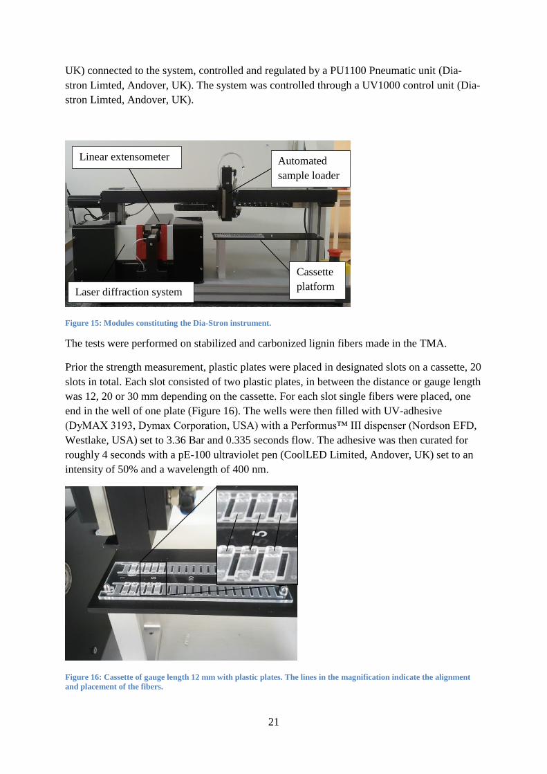
21

UK) connected to the system, controlled and regulated by a PU1100 Pneumatic unit (Dia-

stron Limted, Andover, UK). The system was controlled through a UV1000 control unit (Dia-

stron Limted, Andover, UK).

Figure 15: Modules constituting the Dia-Stron instrument.

The tests were performed on stabilized and carbonized lignin fibers made in the TMA.

Prior the strength measurement, plastic plates were placed in designated slots on a cassette, 20

slots in total. Each slot consisted of two plastic plates, in between the distance or gauge length

was 12, 20 or 30 mm depending on the cassette. For each slot single fibers were placed, one

end in the well of one plate (Figure 16). The wells were then filled with UV-adhesive

(DyMAX 3193, Dymax Corporation, USA) with a Performus™ III dispenser (Nordson EFD,

Westlake, USA) set to 3.36 Bar and 0.335 seconds flow. The adhesive was then curated for

roughly 4 seconds with a pE-100 ultraviolet pen (CoolLED Limited, Andover, UK) set to an

intensity of 50% and a wavelength of 400 nm.

Figure 16: Cassette of gauge length 12 mm with plastic plates. The lines in the magnification indicate the alignment

and placement of the fibers.

Automated

sample loader

Cassette

platform

Linear extensometer

Laser diffraction system

22

The whole cassette was then placed on the cassette holder of the automated tensile testing

system Dia-stron (Dia-stron Limted, Andover, UK). The automated sample loader picked up

the couple of plates and moved the sample to the linear extensometer modulus coupled with

the laser diffraction system. Through light diffraction the diameter was measured, in which

the modulus “rocked” back and forth to find the position where the signal/intensity of the

diffraction was strongest. The laser diffraction system was very sensitive and the software

could not detect/calculate any diameter from the diffraction pattern if the samples were

irregular in form, insufficiently round or transparent. Regardless of whether the diameter

measurements were successful or not the LEX modulus performed, afterwards, an extension

of the fiber till it ultimately broke. From the test the UvWin software (v. 3.35.0000 build 2,

Dia-stron Limted) plotted the stress versus strain in a graph. By using the analytical tool

provided by the same software, the corrected E-modulus could be determined. (The

mathematical models are given above, in section 2.3.1).

The compliance for the system was calculated according the appendix (section 8.2.3.1).

However, the compliance was neglected in the calculations of E-modulus.

The LDS was set to a tension force of 3 gram force (gmf) prior to measurement and to an

extension rate of 0.1 mm/sec. The linear extensometer had a gauge force of 2 gmf prior to

measurement and extended the sample to 7% of the gauge length at 0.1 mm/sec. The

threshold of breakage was set to 5 gmf and the max force allowed was 500 gmf. When the

sample snapped/broke the instrument informed the user by sending out a loud beep noise

where after the automated sample loader arm moved and discarded the sample in the

originating slot and continued to the next slot.

2.4 Thermogravimetric Analysis (TGA) The principles of TGA and used methods are described in the following sections.

2.4.1 Principles

TGA is a thermal analysis in which the specimen is subjected to elevated temperatures. In this

fashion the chemical and physical properties can be determined by measuring the change of

weight as a function of increasing temperature. This provides information about thermal

stability, degradation, decomposition and vaporization of substances. (Coats, Redfern 1963)

In particular, for this project, decomposition in the form of pyrolysis (in inert atmosphere) is

the most interesting aspect.

2.4.2 Method

During carbonization of the stabilized lignin fibers mainly the oxygen and hydrogen content

of the fibers will be reduced, a pyrolysis, meaning that different oxygen containing substances

will be released from the fibers. In order to monitor the change in mass a thermogravimetric

analysis was carried out in a TGA 7 thermogravimetric analyser (PerkinElmer Inc, Waltham,

USA).

A few stabilized fibers were hacked into small pieces and put into a little platinum dish. In

turn the dish was placed on the internal balance of the TGA. The glass cylinder tube was then

elevated so it would contain the sample. In the elevated state gas of pure nitrogen from a

23

Nitrogen 5.0 LAB LINE® N2 (N2 ≥ 99.999%) tube (Strandmöllen AB, Sweden) flowed

through the system. Afterwards the balance was tared and the instrument was then left

untouched alone in the room for a brief moment so that the balance would adjust and stabilize

itself. (The sensitive balance fluctuated and would react to even the slightest movement in the

room.)

The instrument was connected to a TAC 7/DX thermal analysis control unit (PerkinElmer Inc,

Waltham, USA). Via a computer, measurement data of the weight loss was collected by the

Pyris software (v. 8.0.0.0172, PerkinElmer Inc., Waltham, USA) over a set temperature range.

The program was set to run the TGA from 20°C to 1000°C at 10°C/min as the weight was

measured at each point. However, the TGA managed only to reach 885°C before cooling. The

initial mass was 0.6290 mg.

However, TGA-instrument was very unreliable since it provided illogical readings (e.g. some

measurements showed negative mass). This was probably caused by air leaking into the

system, resulting in combustion of the stabilized lignin fibers. In other word the instrument

was not sealed completely and the environment inside the system was not kept inert or oxygen

free.

As a measure, a reference carbonization was done in the TMA-instrument for comparison. 30

fibers, glued together with carbon paint, were weighted on an AE200 balance (Mettler

Toledo, USA) before and after carbonization up to temperatures of 300, 600 and 900°C

(10K/min). Initial masses were 2.7, 2.2 and 2.7 mg respectively for each carbonization

temperature. The results were thought to serve as calibration point for the mass-loss curve in

the TGA. The weight loss graph was corrected accordingly.

As a second measure of obtaining a decent measurement of weight loss, stabilized lignin

fibers were sent to the NETZSCH Applications Laboratory, section of thermal analysis, in

Selb, Germany for investigation, in mission of Innventia AB (Stockholm, Sweden).

Two measurements were performed with the thermogravimetric analyzer, thermo-

microbalance TG 209 F1 Libra® (NETZSCH GmbH, Selb, Germany). Precise internal mass

flow controllers of the vacuum tight instrument and a resolution of 0.1 µg enabled high

precision measurements. For control and data acquisition the PROTEUS® software

(NETZSCH GmbH, Selb, Germany) was employed.

The samples were placed into an Al2O3 crucible, and the system was evacuated and refilled

with nitrogen (20 ml/min) before measurement. The program was set to run from 20°C to

1100°C at 10°C/min as the weight was measured at each point. Initial masses of the both

samples were 1.972 and 2.038 mg.

2.5 Fourier Transform Infrared Spectroscopy (FTIR) The principles of FTIR and used methods are described in the following sections.

24

2.5.1 Principles

Infrared spectroscopy works on the principle that molecules and atoms interact with

electromagnetic radiation. Infrared light causes atoms and groups of atoms to vibrate with

increased amplitude about the connecting covalent bond. (Solomons, Fryhle 2011a)

The vibration or oscillation occurs only at certain frequencies, meaning that the vibrational

states are quantized energy levels. A transition between states can only occur when the

frequency of the radiation match the transition energy (i.e. the frequencies resonate), in which

case the radiation is absorbed by the compound. (Solomons, Fryhle 2011a)

Since different functional groups and molecules are arranged in specific ways, light will be

absorbed at frequencies that correspond to the molecules and functional groups. The

frequency is related to the masses of the bonded atoms and the stiffness of the bond.

(Solomons, Fryhle 2011a)

In order for a molecule to be ‘IR-active’, the dipole moment must change as the vibration

occurs. Thus symmetric molecules, such as homodiatomic molecules (e.g. N2 and O2), does

not absorb IR-light. (Solomons, Fryhle 2011a)

The vibration can occur in a variety of ways: symmetric stretching, asymmetric stretching,

scissoring and twisting etc. (Solomons, Fryhle 2011a)

An IR-spectrometer operates by irradiating a sample with IR-light. The transmittance of the

radiation is compared to the transmittance in absence of sample, a so called reference. The

comparison indicates the frequencies where the sample absorbed light. (Solomons, Fryhle

2011a)

FTIR spectrometers employ a Michelson interferometer. The radiation is split into two beams,

by a beam splitter. The beams are reflected back on two mirrors, of which one is mobile, and

recombine which causes interference. The radiation passes through the sample to the detector

which records the signal as an ‘interferogram’. Through a Fourier transform the interferogram

is then converted into a spectrum. (Solomons, Fryhle 2011a)

The absorption can be observed as a peak in the spectrum where the position is specified in

units of wavenumbers, which is the reciprocal of the wavelength, often expressed as cm-1

.

(Solomons, Fryhle 2011a)

�̅� =1

𝜆

This is due to the energy (∆E) of absorption being directly proportional to the frequency (f)

according the equation:

𝛥𝐸 = ℎ𝑓 =∕ 𝑓 =𝑐

𝜆∕=

ℎ𝑐

𝜆= �̅�ℎ𝑐

25

2.5.2 Method

Fiber samples were carbonized in the TMA prior analysis in FTIR-spectroscopy. The

carbonization temperature and rate was 1000°C and 10 K/min, respectively.

By using an agat mortar the carbonized fibers were grinded thoroughly. Small fragments of

the fibers spurt away when grinding, thus the mortar had to be contained within a hand folded

dome of aluminum foil. This prevented fiber fragments from escaping.

Depending on the degree of carbonization different amount of sample was used when

grinding. The more carbonized the fibers were the less amount had to be used in order to get

distinctive spectrum. The weight of the fiber sample was determined by using a highly

sensitive balance (Ultramicro Type 4504 MP8-1, Sartorius AG, Goettingen, Germany),

measuring weights less than 1 mg, 4 digits precision.

Previously dried for 30 min in a Memmert Type U30 oven (Gemini BV, Apeldoorn,

Netherlands), set to 105°C, potassium bromide (KBr) powder (Uvasol®, Merck Millipore,

Billerica, USA) was added and mixed/grinded together with the sample. The amount was

roughly the same for each sample, i.e. approximately 300 mg.

The mixture was then transferred to a hydraulic press to form a slightly transparent thin black

disc-like pellet, 13 mm in diameter and approximatively 2 mm thick, under pressure of 250

kg/cm2 (recalculated to nearly 250 bar) and slight vacuum (Figure 17). Pellets of lignin

powder, stabilized or carbonized lignin fibers up to 300°C were, instead, somewhat brown in

color. The reference pellet was made in a similar manner with solely KBr powder, 300 mg,

resulting in a clear transparent pellet.

Figure 17: Hydraulic press (top) with pieces (bottom) used to form disc-shaped pellets.

26

Due to the hygroscopic nature of KBr (van der Maas, J. H., Tolk 1962, Abo 2010) the full

procedure had to be done quickly. The pellet was then rapidly inserted with the holder into the

FTIR-spectrometer, since the pellet had the tendency to become “cloudy” rather fast due to it

soaking up moisture directly from the atmosphere.

A Varian 680-IR FTIR Spectrometer (Varian Incorporate, Palo Alto, USA) was used for this

study (Figure 18).

Figure 18: The Varian spectroscopy instrument.

During the FTIR-spectrometry the atmosphere in the sample compartment was continuously

purged with dry nitrogen gas, eliminating substances like carbon dioxide that may interfere

with the spectra. The level of moisture in the gas was regulated by an external filter connected

to the device keeping the atmosphere as dry as possible.

Since the compartment was opened when the sample was inserted into the pellet holder, air

leaked in. By looking at the live spectra, the scan was manually started when the carbon

dioxide peak had disappeared. The time between insertion and spectral scan was estimated to

60 sec.

The spectral resolution was set to 2 cm-1

and the sample was scanned in range 4000-600 cm-1

.

A thermo electric (TE) cooled DLaTGS (deuterated L-alanine doped triglycene sulphate)

detector was used to collect the absorbance data at 5 kHz frequency. The samples were

illuminated by a mid-infrared source (MIR) and the beam splitter was of KBr.

Both the background and samples were scanned 32 times each. One background spectra was

made (150115) and used for all the samples throughout the study. However, it should be noted

that the correct procedure is to collect a background spectrum for each measurement,

preferable as close to the measurement as possible.

The collected spectrums were visualized in the Varian Resolutions Pro software (v.5.1.0.829,

Varian Incorporate, Palo Alto, USA).

27

2.6 Scanning Electron Microscope (SEM) The principles of SEM and used methods are described in the following sections.

2.6.1 Principles

The principle behind electron microscope is bombarding a surface of a specimen with a

stream of electrons. The scattering of the electrons can be used to generate an image of the

scanned area.

The electrons are produced by an electron gun which consists of an electron source (usually

tungsten), called cathode, and an electron accelerator. There are different methods to generate

the electrons from the cathode. In a field emission gun, the principle of field emission is

utilized. I.e. the electrostatic field at the tip of the cathode is increased to the point that the

potential barrier becomes small enough to allow electrons to escape through this barrier by

quantum-mechanical tunneling. After emission the electrons are accelerated in an electric

field, parallel to the optic axis, to a final kinetic energy. (Egerton 2005)

An objective in the SEM condenses the incident beam into a so called electron probe,

typically 10 nm in diameter. The beam is scanned over a rectangular area of the specimen,

known as raster scanning. (Egerton 2005)

Figure 19: Elastic and inelastic scattering. The electrons are incident from above, indicated by arrows.

Primary electrons from the incident beam penetrate the specimen and scatter both elastically

and inelastically (Figure 19). The respective scattering is caused by interaction with the

nucleus or with electrons surrounding the nucleus. Primary electrons that backscatter (i.e.

scattering through an angle greater than 90° to the incident beam) can be collected by a

backscattering detector placed above the specimen. The signal increases with atomic number

and thus contrast between chemical compositions can be observed in the imaging of materials.

(Egerton 2005)

28

Through inelastic interaction and transfer of kinetic energy, primary electrons cause ejection

of electrons orbiting around the nucleus. As moving particles, the secondary electrons

themselves will interact with other atomic electrons and scatter inelastically, gradually losing

kinetic energy until most of them are brought to rest within the material. Secondary electrons

that instead escape close to the surface are collected for imaging by an Everhart-Thornley

detector. Hence the image is a property of the surface structure (topography) and displays

topographical contrast. (Egerton 2005)

The same inelastic effect that ‘knock out’ electrons (in other words causes the electrons to

undergo transition to a higher energy state) in the inner shell (e.g. K-shell), results in a

vacancy in the shell. An electron in a higher shell de-excite, in a downward energy transition,

to fill the hole. The transition causes release/emission of energy in form of photons with

wavelengths in the X-ray spectrum. Since the X-rays are characteristic to atomic species, it

allows for measurement of the elemental composition of the specimen. A silicon drift detector

is often used to detect the X-rays. (Egerton 2005)

Transition to the innermost shell is called K-emission and is denoted α if the electron de-

excite from the L shell, β from the M shell etc. Similarly, transition between the M and L

shell would result in Lα-emission. (Egerton 2005)

2.6.2 Method

A few stabilized and carbonized lignin fibers from the TMA carbonization process were

selected for imaging and X-ray analyses. The analysis was carried out using a scanning

electron microscope (Quanta FEG 650, FEI™, USA) combined with an energy dispersive X-

ray spectrometer (EDS) (Figure 20). The instrument was located in the Department of

Geological Sciences at the Stockholm University.

Figure 20: The scanning electron microscope, Quanta FEG 650.

Main components of the instrument include a field emission gun (FEG), a concentric

backscattered electron detector (CBS) and an EDS with a silicon drift detector (SDD) (X-Max

29

silicon X-ray, Oxford Instruments). The instrument was operated through the AZtec software

(Oxford Instruments).

Prior the study, the fiber samples were attached to the sample holders with double coated

PELCO carbon tape (Ted Pella Inc., Redding, USA). Parts of the axial fiber surface and fiber

cross-section was imaged and analyzed of content. In the former, the fibers were positioned

horizontally on the holder and in the latter the fibers were positioned vertically in a special

holder.

The following day the fiber samples were placed inside the SEM chamber which was

evacuated of atmosphere to a pressure of approximatively 1 mbar. The system operated at an

accelerating voltage of 15 kV and a working distance (WD) of 10 mm and the fibers could be

observed in 1000-5000 times magnification.

2.7 Light Microscopy Prior and after carbonization treatment in the TMA a light microscope (Axioplan 2 Imaging,

Carl Zeiss) was used to look at the structure, integrity, to measure diameter changes and to

spot defects. Placed on top of the microscope was a CT5 camera (ProgRes®, Jenoptik AG,

Jena, Germany) which was used to capture images of the fibers in the computer software

Capture Pro 2.8.8 (ProgRes®, Jenoptik AG, Jena, Germany).

The fibers were simply put on a microscope slide which was placed under the microscope and

illuminated from above. The magnification was 10, 20 or 50x and the camera captured the

images in resolution of 2592x1944 and 1296x972 2x Bin. In the software the diameters was

be measured by drawing a straight perpendicular line between two opposite points of the fiber

contour.

30

3 Results In the following section the outcome of each experiment is described.

3.1 TMA The TMA provided information about the behavior of stabilized lignin fibers in temperature

changes and under static or varied load during carbonization. Each sample is represented by

one carbonization in the TMA instrument.

The data from the carbonization is presented as linear dimensional change over temperature or

time.

3.1.1 Static measurement

By studying the expansion/contraction (red curve) in Figure 21, where the slope/derivative

(blue curve) is represented as the linear expansion coefficient α, we can observe a slight

expansion up to 250°C, followed by a fast shrinkage. Thereafter the rate of contraction

diminishes slightly around 420°C and continues in a linear fashion until it begins to disappear

around 700°C. After 1100°C the slope cease completely, as illustrated in Figure 22 and Figure

23, where some of the samples have been carbonized further.

Figure 21: Deformation of approximatively 50 fibers, 20 mm each, during carbonization to 1000°C at 1 K/min and 5

mN load. The red curve represents the length changes, while the blue curve represents the slope/alpha value of the

blue curve.

Hereafter, the carbonization in Figure 21 will be referred to as the standard carbonization,

since it represents the general deformation pattern of all fibers. It is color marked as red in the

following charts, allowing for easy comparisons.

-0.0010

-0.0005

0.0000

0.0005

-25%

-20%

-15%

-10%

-5%

0%

5%

0 100 200 300 400 500 600 700 800 900 1000 1100 1200

α (

1/K

)

∆L/

L 0

Temperature (°C)

31

Carbonizations of stabilized fibers with different lengths are compared in Figure 22. The

curves follow approximatively the same path. There is no clear difference between 15 and 20

mm fibers. However, the curve of 10 mm deviates from the path and possess a nick around

600°C (possibly due to a fiber or multiple fiber breaking). The final difference, after

completion, is around 2 percentage units compared to the 15 and 20 mm fiber samples.

Figure 22: Comparison of samples with varying lengths. The number of fiber in the samples, corresponding to the

blue, green and red curve, was respectively 10, 20 and 50. The blue curve possesses a nick around 600°C. The

carbonization was performed at 1 K/min, under load of 5 mN.

The following Figure 23 is compiled of sample data with varied amount of fibers. We can see

that the majority of the curves fall into the same path.

-25%

-20%

-15%

-10%

-5%

0%

5%

0 100 200 300 400 500 600 700 800 900 1000 1100 1200

∆L/

L 0

Temperature (°C)

10 mm

15 mm

20 mm

32

Figure 23: Carbonizations of samples with varying amount of fibers. The triangles indicate where the fibers broke,

slipped out from the clamps or where the length exceeded the TMAs limit of measurement. The missing segments

between 200-300°C are also due to the latter. The red curve (50 fibers) is from Figure 21 and is here represented as a

reference. The carbonization was performed at 1 K/min, under load of 5 mN.

In particular, samples with 50 fibers lie close together, whereas the 20- and 10-fiber-samples

are more likely to deviate from the path. The standard carbonization curve (Figure 21) is

drawn into the middle.

Figure 24 depicts the elongation of samples at different rates of increasing temperature, 1, 10,

20 and 40 K/min. The respective deformation at 1 K/min and 40 K/min differ little to each

other. However, the curve of 40 K/min may be a little smoother than that of 1 K/min. It is

apparent that the curves follow the same pattern, although the pairs (1 and 40 K/min

respective 10 K/min and 20 K/min) have an offset to each other.

-30%

-25%

-20%

-15%

-10%

-5%

0%

5%

0 200 400 600 800 1000 1200

∆L/

L 0

Temperature (°C)

10 fibers

20 fibers

50 fibers

33

Figure 24: Comparison between carbonizations at 1, 10, 20 and 40 K/min under load of 5 mN. The sample amount

was 50 fibers, 20 mm in length. The blue curve of 40 K/min may be slightly smoother than the red curve of 1K/min.

The green curve of 10 K/min and orange curve of 20 K/min have no noticeable differences, except that the latter has

shrunk slightly more. The curves of 10 and 20 K/min respective 1 and 40 K/min are offset to each other. The missing

segments is due to the length signal exceeding the TMAs limit of measurement, hence the data is missing.

Put into a different perspective, the curves of 10, 20 and 40 K/min are illustrated as

deformation over time in Figure 25, accompanied with the change of temperature over time.

The heating appears to be faster in the beginning despite the specified rate in the

carbonization program. Not until after 200°C had the rate been corrected to match the

program. However, the different rates of heating seemingly do not affect the deformation of

the fiber samples.

-25%

-20%

-15%

-10%

-5%

0%

5%

0 100 200 300 400 500 600 700 800 900 1000 1100 1200 1300

∆L/

L 0

Temperature (°C)

1 K/min

10 K/min

20 K/min

40 K/min

34

Figure 25: The elongation as well as temperature in the TMA sample holder is visualized over time. The rate of

heating is faster prior 200°C.

0

100

200

300

400

500

600

700

800

900

1000

1100

1200

1300

-25%

-20%

-15%

-10%

-5%

0%

5%

0 20 40 60 80 100 120 140

Tem

pe

ratu

re (

°C)

∆L/

L 0

Time (min)

10 K/min

20 K/min

40 K/min

35

3.1.2 Measurements with increasing force

The result of increasing the force applied to the fiber samples are presented in this section.

Each sample of 5 fibers was carbonized at 10 K/min up to 1000°C. They were attached with

graphitic adhesive to graphitic plates, serving as clamps. The entire setup, of plates, adhesive

and fibers, were put in an oven for curing of the adhesive.

The samples (Table 2) are marked with letters since we will evaluate the strength performance

of these in the section below (3.2.2). The TMA-deformation curve of sample Z can be found

in the appendix (8.2.1).

Table 2: Displaying the range of temperature and force of sample A-L and Z along with amount of fiber.

Sample Force range (N)

Temperature (°C)

Rate (mN/K) Fiber amount

A 0.01-0.3 375-975 0.48 5

B 0.01-0.4 350-950 0.65 5

C 0.01-0.5 350-950 0.82 5

D 0.01-0.1 450-550 0.90 4

E 0.01-0.2 450-550 1.9 5

F 0.01-0.2 400-600 0.95 5

G 0.01-0.35 300-900 0.57 5

H 0.01-0.07-0.35 300-390-850 0.67, 0.61 5

I 0.01-0.12-0.6 300-420-820 0.92, 1.2 10

J 0.01-0.083-0.6 300-390-770 0.81, 1.4 10

K 0.01-0.083-0.6 300-390-770 0.81, 1.4 10

L 0.01-0.07-0.35 300-420-820 0.5, 0.7 5

Z 0.005-0.4 500-700 2.0 10

In the following Figure 26, the carbonization and elongation of three samples (A-C), under

same parameters (10 K/min and 5 fibers in each sample), is shown. The force is continuously

increased from 10 mN to 30, 40 and 50 mN, starting at 375°C, 350°C and 350°C and ending

at 975°C, 950°C and 950°C, respectively for sample A-C. As illustrated by the figure, the

contraction of the fiber is inhibited by applying an increasing amount of force. If compared to

the standard carbonization curve (Figure 21), which had a final contraction of nearly 21 % of

the initial length the contraction here is significantly smaller. The stabilized fibers of sample

A-C shrunk to 9, 7 and 3 %, respectively.

36

Figure 26: Carbonization with ramped force. The solid line is the elongation of the sample (A-C) while the dashed line

is the force applied to each sample. The blue, red and green curves belong respectively to sample A, B and C. The rate

of heating was 10 K/min and the amount of fibers was 5.

The effects of starting temperatures and rate of force ramp are studied in Figure 27. The

samples (D-G), of 5 fibers each, underwent carbonization at 10 K/min. For each carbonization

the force ramp was successively put at an earlier temperature, 450, 400, 400 and 300°C for

sample D-G, respectively.

Although, the final force for sample D-F is lower than that for sample A-C in Figure 26, the

deformation is seemingly the same at 12, 6 and 3 % for sample D, E and F, respectively. This

is because the temperature interval wherein the force can increase is kept small, and the slope

of the ramp is bigger, hence the force is already reasonably high at early temperatures

compared to sample A-C where the same forces are reached at higher temperatures.

However, one difference is that this setting of force results in a broad peak in the curves

around 550°C, in particular the curves E and F. In a usual fashion, the fibers expand up to

250°C and then contract. But progressively, the fibers internal force of contraction cannot

compete with the applied force of the TMA anymore and thus expand. After 550°C the

internal force becomes the winning competitor of the forces again and the fibers start to

contract once again. The contraction is not only dependent on the tension (stress) but also on

the stiffness (E-modulus) of the fibers. Initially the stiffness is relatively low, but as it starts to

increase around 400°C, as the temperature in the carbonization is continuously increased, the

contraction will be more and more affected by the increasing stiffness.

This behavior is also visible in the curve of sample D, although the force of the TMA is not

high enough to withstand the contraction we can see that the applied force suppress the

contraction by a moderate amount.

0.00

0.10

0.20

0.30

0.40

0.50

0.60

-15%

-10%

-5%

0%

5%

0 100 200 300 400 500 600 700 800 900 1000 1100

Forc

e (

N)

∆L/

L 0

Temperature (°C)

C B A

0.01-0.05 N 0.01-0.04 N 0.01-0.03 N

37

In the curve of sample G the force ramp is similar to those in Figure 26 in terms of rate and

final value. In contrast to the previous carbonizations of samples A-F the ramp starts earlier at

300°C which causes a longer expansion of the fibers. The nick in the curve, due to a fiber

breaking, may tell us that the applied force is too strong in this moment. However, due to this

fiber breakage, the remaining fibers does not contract more than the equivalent amount of the

expansion, the fibers stays close to 0 % deformation. When accounting for the force per fiber

the stress increases for the remaining fibers when one fiber breaks.

Figure 27: The ramping of force at different starting temperatures. The samples D-G, of 5 fibers each, were

carbonized at 10 K/min Earlier starting temperatures seems to suppress the shrinkage. The nick in curve of G around

500°C is possibly due to a fiber breaking.

The samples A, G and H are compared in Figure 28. The force ramps are almost the same for

each sample. However, the ramping of the force starts earlier in the carbonization of G and H.

This results in contractions that are less than that of sample A.

The force is stronger in the carbonization of sample G than H. Even so, the curve of sample G

is kept above curve H. In reality, curve G should follow the same path since the force differs

only slightly between the carbonizations. The breakage of one fiber, observed as a nick in the

G curve, results in a higher stress on each remaining fiber which might explain why curve G

is above H.

0.00

0.05

0.10

0.15

0.20

0.25

0.30

0.35

0.40

-15%

-10%

-5%

0%

5%

0 100 200 300 400 500 600 700 800 900 1000 1100

Forc

e (

N)

∆L/

L 0

Temperature (°C)

G F E D

0.01-0.35 N 0.01-0.2 N 0.01-0.2 N 0.01-0.1 N

38

Figure 28: Comparison between samples A, G and H. The force ramp is similar for each carbonization. However, the

ramp starts earlier in the carbonization of sample G and H. The force ramp in carbonization of sample H was divided

into two parts, first up to 0.07 N between 300 and 390°C then to 0.35 between 390°C and 850°C.

The next figure depicts the deformation of 10 fibers (Figure 29). The force was doubled to

match the carbonization of 5 fibers. We can observe a pattern similar to that of sample H in

both curves in Figure 28. The final deformation stays around the same at 6 % contraction of

the initial length, whereas sample H ends at 7 %. The force ramp was divided into two parts,

for sample I the force was increased to 70 mN at 420°C whereas the force in sample J was

increased to 83 mN at 390°C. In the second stage the force was increased to 600 mN at 820°C

for sample I and 770°C for sample J.

Figure 29: Carbonizations of samples with 10 stabilized fibers. Both curves differ little to each other. However, curve

J deviates unexpected from the path around 700°C, possible due to a fiber breaking. A nick around 300°C can also be

observed.

0.00

0.05

0.10

0.15

0.20

0.25

0.30

0.35

0.40

-10%

-5%

0%

5%

0 100 200 300 400 500 600 700 800 900 1000 1100

Forc

e (

N)

∆L/

L 0

Temperature (°C)

G

A

H

0.01-0.07-0.35 N 0.01-0.35 N

0.00

0.10

0.20

0.30

0.40

0.50

0.60

0.70

-10%

-5%

0%

5%

0 100 200 300 400 500 600 700 800 900 1000 1100

Forc

e (

N)

∆L/

L 0

Temperature (°C)

J I

0.01-0.07-0.6 N 0.01-0.083-0.6 N

39

The sample K and L contains 10 respectively 5 fibers. Figure 30 illustrates the difficulty of

applying force on the samples. The force ramp was divided into two parts, for sample K the

force was increased to 83 mN, 390°C, whereas the force in sample L was increased to 70 mN,

420°C. In the second stage the force was increased to 600 mN, 770°C, and 350 mN, 820°C,

respectively for sample K and L.

Stabilized fibers are in the region of 300-500°C very susceptible to force, this is the reason

they easily break when ramping the force. The curve of sample K is almost straight up till the

breakage.

Figure 30: Successful carbonizations compared to failed carbonizations when applying force. The triangles indicate

where the fiber bundle broke.

3.2 Dia-stron Uniaxial tensile testing was performed on the lignin fibers, carbonized in the TMA-instrument

through different programs, by the Dia-Stron instrument.

3.2.1 Evaluation of temperature and heating rate

In terms of mechanical performance, the significance of final temperature (i.e. 300°C, 400°C,

and so on up to 1300°C) and heating rates (1, 10, 20 and 40 K/min) of the lignin fiber

carbonization is evaluated in this section.

Starting with the carbonization temperatures, we can observe in Figure 31 that the fibers

become stronger with increasing carbonization temperature. The rate of heating was kept at

10 K/min during the carbonization and the gauge length in the Dia-Stron measurement was 12

mm.

0.00

0.10

0.20

0.30

0.40

0.50

0.60

0.70

-10%

-5%

0%

5%

0 100 200 300 400 500 600 700 800 900 1000 1100

Forc

e (

N)

∆L/

L 0

Temperature (°C)

K L

I J

0.01-0.083-0.6 N 0.01-0.07-0.6 N 0.01-0.07-0.6 N 0.01-0.07-0.35 N

40

Stabilized lignin fibers (non-carbonized) and fibers carbonized to 500°C tend have a low

tensile strength below 200 MPa. The fibers are however still more susceptible to

deformation/extension before breaking. Plastic behavior is also hinted by the curvature of

these fibers in the diagram.

As the temperature increases we observe that the fibers become stiffer and the curves become

more and more linear in shape. The slope, which account for the E-modulus, increases as well

and reaches its maximum above 900°C. At which point the tensile strength is above 600 MPa.

Figure 31: Strain versus stress. The dip indicates the breakpoint of the fiber samples, at which point the stress account

for the ultimate tensile strength. Each sample was carbonized at 10 K/min and the gauge length was 12 mm.

Figure 32 present the E-modulus taken from measurements of lignin fibers carbonized at 1

K/min to different final temperatures (300°C, 400°C… and 1200°C). At least 4 points of data

are plotted in each temperature. The data at 25°C mark stabilized lignin fibers (non-

carbonized).

The red curve in the diagram provides a picture about how the average E-modulus changes.

As the carbonization temperature increases, the E-modulus increases. The maximum is

observed at 1000°C and thereafter the E-modulus inclines slightly. Consider, however, that

the data in each temperature may be insufficient for an accurate picture since the points are

widely spread, especially at 1000°C and forward.

0

100

200

300

400

500

600

700

800

0 0.5 1 1.5 2 2.5 3 3.5 4 4.5

Stre

ss (

MP

a)

Extension (%)

400°C 300°C

1300°C 1200°C 1100°C 1000°C 900°C 800°C 700°C 600°C 500°C

Stabilized Lignin

41

Figure 32: Representation of how the E-modulus increases with temperature. A (red) line is drawn between the

average points, calculated from the data points (blue) in each temperature. The error bars in each temperature

represent the sample standard deviation. The tested fibers were carbonized at 1 K/min.

Figure 33 is informative regarding how the tensile strength improves as the carbonization

temperature increases. The data of tensile strength was acquired from the same measurement

as above. In contrast to the E-modulus, the increasing of tensile strength may not be as clear.

The average line in red fail to show a smooth curve, compared to the E-modulus of the points.

The tensile strength is kept at relatively low values up to 600°C. Then it makes a drastic jump

at 700°C. For the following temperatures it is difficult to evaluate whether the tensile strength

increases or not, since the points are widely spread, even more than in the previous figure.

0

10

20

30

40

50

60

0 100 200 300 400 500 600 700 800 900 1000 1100 1200

E-m

od

ulu

s (G

Pa)

Temperature (°C)

42

Figure 33: Tensile strength plotted against temperature. A (red) line is drawn between the average points, calculated

from the data points (blue) in each temperature. The error bars in each temperature represent the sample standard

deviation. The tested fibers were carbonized at 1 K/min.

Similarly, a series was made to evaluate the influence of 10 K/min on E-modulus and tensile

strength (Figure 34, Figure 35).

Although a fewer data points are used in the diagrams, the same behavior can be observed; the

E-modulus increase with increasing temperature and the tensile strength also becomes higher

(However, with an increasing margin of error as previously).

0

100

200

300

400

500

600

700

800

900

0 100 200 300 400 500 600 700 800 900 1000 1100 1200

Ten

sio

n S

tren

gth

(M

Pa)

Temperature (°C)

43

Figure 34: E-modulus plotted against temperature. A (red) line is drawn between the average points, calculated from

the data points (blue) in each temperature. The error bars in each temperature represent the sample standard

deviation. The tested fibers were carbonized at 10 K/min.

Figure 35: Tensile strength plotted against temperature. A (red) line is drawn between the average points (red

squares), calculated from the data points (blue) in each temperature. The error bars in each temperature represent

the sample standard deviation. The tested fibers were carbonized at 10 K/min.

0

10

20

30

40

300 400 500 600 700 800 900 1000 1100 1200 1300

E-m

od

ulu

s (G

Pa)

Temperature (°C)

0

100

200

300

400

500

600

700

800

900

1000

300 400 500 600 700 800 900 1000 1100 1200 1300

Ten

sile

Str

en

gth

(M

Pa)

Temperature (°C)

44

The E-modulus and tensile strength values with averages from every carbonization (at 1, 10,

20 and 40 K/min) are displayed in the following charts (Figure 36, Figure 37).

Figure 36: E-modulus plotted against temperature. Contains all data points from all samples carbonized in every rate.

The plotted lines illustrate how the average E-modulus changes over temperature. The error bars in each temperature

and for each heating rate represent the sample standard deviation.

Figure 37: Tensile strength plotted against temperature. Contains all data points from all samples carbonized in every

rate. The drawn lines illustrate how the average tensile strength progresses over carbonization temperature. The

error bars in each temperature and for each heating rate represent the sample standard deviation.

0

10

20

30

40

50

0 100 200 300 400 500 600 700 800 900 1000 1100 1200 1300

E-m

od

ulu

s (

GP

a)

Temperature (°C)

1K/min

10K/min

20K/min

40K/min

0

100

200

300

400

500

600

700

800

900

300 400 500 600 700 800 900 1000 1100 1200 1300

Te

nsi

le S

tre

ngt

h (

MP

a)

Temperature (°C)

1K/min

10K/min

20K/min

40K/min

45

The progression of tensile strength over temperature is still hard to evaluate, since the points

in each temperature have a large spread. The spread of points cause a large margin of error

and evaluation must be considered with caution.

The averages of each rate are summarized in the tables below (Table 3, Table 4).

Table 3: An overview of the average E-modulus for the most interesting carbonization temperatures. The values are

displayed in units of GPa. The sample standard deviation is displayed in parenthesis.

1 K/min 10 K/min 20 K/min 40 K/min

900°C 34 (2.2) 34 (1.9) 30 (N/A) 31 (0.86)

1000°C 37 (3.7) 35 (3.2) 36 (0.83) 35 (1.4)

1100°C 37 (9.4) 34 (2.5) 35 (2.4) 36 (2.1)

1200°C 35 (4.1) 32 (0.37) 32 (2.5) 34 (0.88)

1300°C N/A 33 (2.9) 36 (3.3) 38 (1.2)

Table 4: An overview of the average tensile strength for the most interesting carbonization temperatures. The values

are displayed in units of MPa. The sample standard deviation is displayed in parenthesis.

1 K/min 10 K/min 20 K/min 40 K/min

900°C 420 (76) 550 (59) 430 (N/A) 470 (74)

1000°C 600 (240) 640 (80) 590 (88) 570 (51)

1100°C 500 (76) 700 (230) 650 (130) 300 (69)

1200°C 460 (190) 590 (74) 550 (56) 620 (6.9)

1300°C N/A 660 (64) 550 (130) 650 (220)

3.2.2 Evaluation of applied force during carbonization

In terms of mechanical performance, the significance of applied force on the stabilized lignin

fiber during carbonization is evaluated in this section. The samples, mainly A-H, that

underwent carbonization, as shown in section 3.1.2, were tested in the Dia-Stron system and

the result is presented here. (The deformation of sample Z during carbonization can be found

in appendix 8.2.1). Fibers that were initially broken prior carbonization served as reference in

the Dia-Stron testing. They showed strength properties characteristic with samples carbonized

under static load.

In short, strong connections between the strength and deformation can be drawn.

46

Table 5: An overview of the interesting samples with average E-modulus and tensile strengths. The sample standard

deviation is displayed in parenthesis. See Table 2 in section 3.1.2 for additional information. The TMA data of the

carbonization of Z can be found in the appendix.

Sample Force range (N)

Temperature (°C)

Average E-mod (GPa)

Average Breakpoint (MPa)

A 0.01-0.3 375-975 49 (2.4) 160 (57)

B 0.01-0.4 350-950 47 (4.0) 760 (150)

C 0.01-0.5 350-950 51 (0.96) 660 (120)

D 0.01-0.1 450-550 39 (2.2) 570 (120)

E 0.01-0.2 450-550 49 (0.40) 550 (100)

F 0.01-0.2 400-600 49 (1.5) 660 (140)

G 0.01-0.35 300-900 51 (6.3) 820 (36)

H 0.01-0.07-0.35 300-390-850 46 (1.1) 600 (73)

Z 0.005-0.4 500-700 38 (7.9) 490 (84)

The first diagram, Figure 38, provides a quick graphical overview of the E-modulus data

shown in Table 5. All samples except for D and Z show a higher value if compared to the E-

modulus without increasing load (recall Table 3 and Table 4).

Figure 38: E-modulus for sample A-H and Z.

If the E-modulus is plotted against tensile strength of every sample, including the samples

carbonized at static load, the samples can be categorized into groups. The following figure

shows all data obtained from the tensile testing (Figure 39). (Note however that tensile

strength and E-modulus in general do not correlate, in other words they do not necessarily

relate to each other. The figure is merely to compare the values of each sample and categorize

them.)

0

10

20

30

40

50

60

A B C D E F G H Z

E-m

od

ulu

s (G

Pa)

47

Figure 39: All obtained data from samples carbonized under static respectively non-static carbonization. The static

carbonized samples are indicated by rate 1, 10, 20 and 40 K/min. All samples were carbonized to 1000°C and the non-

static samples in a rate of 10 K/min.

Although the data from non-static carbonization (letters) is more spread it clearly belongs to a

different group, farther away from the static carbonization cluster (diamonds, ♦). An

exception to that is the D and Z sample, which show no mechanical improvements in contrast

to the other samples and can thus be grouped with the static carbonization. The fibers of

sample A show surprisingly low tensile strength whereas the E-modulus is better than that of

the static carbonized samples. Samples of G and C are relatively close to each other and are

placed farthest away from the static carbonized group.

3.3 TGA The thermogravimetric analysis provided information about the weight loss of stabilized

lignin fibers during carbonization.

Figure 40 displays the measurement made at Innventia AB, where the pale blue line

represents the original measurement and the darker blue line the corrected version. The data

was corrected according calibration points provided by three carbonizations in the TMA-

instrument (300, 600 and 900°C at 10K/min each). Complete calculations and calibrations can

be found in appendix (8.2.2).

Nicks, dents and sudden steps in the curves are evident and are probably caused by vibrations

and motions near the instrument, since the balance was extremely sensitive. The result must

be considered with caution because combustion occurred of the stabilized lignin fibers, due to

air leaking in.

A

A

B

B

B

C

C

C

C

C

D

D

D

D

D

E

E F

F

F

G

G G

H

H H

H

H

Z

Z

I

Y

0

100

200

300

400

500

600

700

800

900

1000

30 35 40 45 50 55 60

Ten

sile

Str

en

gth

(M

Pa)

E-modulus (GPa)

1K/min

10K/min

20K/min

40K/min

48

Aside from that, the figure provides an approximate view of the weight loss over temperature.

Although a residual mass below 30% is not reasonable. The corrected curve is more reliable,

showing a residual mass of 53 %.

Figure 40: TGA measurement of stabilized lignin fibers. (Pale blue) original curve and (strong blue) corrected curve.

The initial mass was 0.6290 mg.

To get a more reliable TGA measurement, stabilized lignin fibers were sent to NETZSCH

GmbH in Selb, Germany, for investigation. The result of the two measurements is shown in

Figure 41.

The data suggest that the weight loss occur in three steps. The first step shows a mass loss of

around 25 % of both samples. The maximum loss rate for this step can be observed in the

derivative curve (DTG, derivative thermogravimetry) around 425°C. The following step is

around 15% mass loss and the derivate peaks at around 560°C. The last step is about 3 % and

the DTG peak is found at 785°C. The residue mass for both samples is about 55%,

corresponding nicely with the corrected curve of the TGA-measurement at Innventia AB.

0

10

20

30

40

50

60

70

80

90

100

0 100 200 300 400 500 600 700 800 900 1000

We

igh

t (%

)

Temperature (°C)

Corrected Weight loss

Weight loss Residue mass:

53% 25%

49

Figure 41: TGA measurements of two samples (blue and green). The TG (thermogravimetry) curve shows the mass

loss over temperature while the derivative of this curve is provided by the DTG (derivative thermogravimetry) curve.

The initial mass of the blue and green sample was 1.972 and2.038 mg, respectively.

In comparison, our TGA-measurement shows a convex shape during the mass loss (between

450 and 750°C) whereas the NETSCH measurement is completely sigmoidal.

Combining the data from the TGA and TMA, the change of diameter of single fibers can be

calculated, assuming that the volume changes in the same manner as the mass. The

assumption is however not entirely true, since the volume change is also caused by sintering

of the stabilized lignin fibers. But it provides with an approximate understanding how the

diameter progresses over carbonization temperature (Figure 42).

The diameter change is compared with static and non-static TMA carbonization. Recall the

deformation of fiber sample G (Figure 28) and the deformation in the standard carbonization

curve (Figure 21). The fibers of sample G are subjected to an increasing force and the

diameter changes more than that of the fibers carbonized under static load. The pattern are

derived from the TGA measurements, at Innventia AB respectively NETZSCH (Figure 40 and

Figure 41).

50

Figure 42: The change of diameter during carbonization of sample G (blue) and the sample of the standard

carbonization curve (red). (Diamonds and triangles) indicate data calculated from the TGA measurement at

NETZSCH while (X) are calculated from the TGA measurement at Innventia AB. The lines represent the force

applied on each sample. The standard carbonization and carbonization of sample G was performed at 1 respectively

10 K/min to 1000°C. Initial diameter was 47 µm.

In turn, the diameter can be recalculated into cross-sectional area of single fibers. By using the

area and force, the change of individual stress of the fibers, during the carbonization in the

TMA-instrument, can be calculated for sample G and the standard carbonization, respectively

(Figure 43 and Figure 44). As mentioned, the full calculations are found in appendix 8.2.2.2.

The breakage of one fiber in the carbonization of sample G (occurs around 500°C, recall

Figure 27) has been taken into consideration when calculating the stress in Figure 43.

Note that the stress scale differs in Figure 43 and Figure 44.

0.00

0.05

0.10

0.15

0.20

0.25

0.30

0.35

0.40

60%

70%

80%

90%

100%

0 100 200 300 400 500 600 700 800 900 1000 1100

Forc

e (

N)

Dia

me

ter

Temperature (°C)

Blue: carbonization G Red: standard carbonization

51

Figure 43: Change of stress during the carbonization of sample G under increasing force. (Diamonds) indicate data

calculated from the TGA measurement at NETZSCH while (X) are calculated from the TGA measurement at

Innventia AB. The breakage of one fiber at 500°C has been taken into account. The carbonization was performed at

10 K/min to 1000°C.

Figure 44 Change of stress during the standard carbonization. (Diamonds) indicate data calculated from the TGA

measurement at NETZSCH while (X) are calculated from the TGA measurement at Innventia AB. The carbonization

was performed at 1 K/min to 1000°C.

0.00E+00

2.00E+07

4.00E+07

6.00E+07

8.00E+07

1.00E+08

0 100 200 300 400 500 600 700 800 900 1000 1100

Stre

ss (

Pa)

Temperature (°C)

4.00E+04

6.00E+04

8.00E+04

1.00E+05

0 100 200 300 400 500 600 700 800 900 1000 1100

Stre

ss (

Pa)

Temperature (°C)

52

3.4 FTIR Infrared spectroscopy was used to study the molecular changes that take place within lignin

fibers during carbonization. Samples that was carbonized to temperatures of 300, 400…

1200°C at 10 K/min were analyzed.

Since many volatile substances evaporate during pyrolysis, the study will mainly focus on the

loss of functional groups and molecules. This will hopefully give an idea of how the

structure/conformation is affected.

Figure 45 shows FTIR-spectra of pulverized and stabilized lignin, respectively. (Lignin

powder is the starting material when spinning fibers. It is melted and extruded into lignin

fibers, followed by stabilization.) Since no valuable information exists in the region of 1800-

2800 cm-1

, all spectra have been cropped. The section above 3000 cm-1

has also been removed

where a broad band 3100-3700 cm-1

with strong intensity was found. The band at that region

is attributed to O-H vibrations which probably indicate that water is present in the KBr-pellet.

It is also coupled with the peak at 1640 cm-1

. Furthermore, the absorption intensities in each

spectrum have been divided by the amount of sample used and all spectra have been baseline

corrected.

The spectroscopic study was hindered or limited by the fact that carbon fibers have a high

tendency of absorbing light (Boccara et al. 1997). The higher degree of carbonization, the

more the lignin fibers absorbed. In fact, amounts higher than 0.3 mg resulted in absorption

levels above 50 % for all frequencies at 900°C, which covered interesting peaks and features

completely. An implication of this was to use extremely low sample amounts as the

carbonization temperature rose. Unfortunately, the spectra become noisy at higher

temperatures as a result from this.

Figure 45: FTIR-spectra of pulverized and stabilized lignin, 3 mg sample per 300 mg KBr.

0

0.05

0.1

0.15

0.2

0.25

0.3

0.35

7009001100130015001700190021002300250027002900

Ab

sorp

tio

n

cm-1

Stabilized Lignin

Pulverized Lignin

53

Table 6: Assignment of bands of softwood lignin in the middle infrared region.

Peak (no.) Frequency of

absorption bands (cm-1)

Assignment/Interpretation

1 1695-1720 C=O stretch in unconjugated ketones, carbonyl, and in ester groups (Derkacheva, Sukhov 2008); conjugated aldehydes and carboxylic acids around and below 1700

cm-1 (Faix 1991) 2 1600 Aromatic skeletal vibration + C=O stretch (Faix 1991, Hergert 1960, Pandey 1999)

3 1515 Aromatic skeletal vibrations (Faix 1991, Hergert 1960)

4 1450-1465 C-H deformation, asymmetric deformation in -CH3 and -CH2- (Faix 1991)

5 1430 Aromatic ring stretching combined with C-H in plane deformation (Faix 1991)

6 1365-1370 Bending vibrations of C–H bond in C–CH3, in-plane bending vibrations of phenolic O–H groups (Faix 1991, Derkacheva, Sukhov 2008)

7 1270 Stretching of guaiacyl rings with C=O groups (Faix 1991, Derkacheva, Sukhov 2008, Agarwal, McSweeny & Ralph 2011)

8 1210-1220 C-C, C-O and C=O stretch; aromatic phenol (Faix 1991, Pandey 1999)

9 1205 Vibrations of aryl–O in aryl–OH and aryl–O–CH3 (Karmanov, Derkacheva 2013); vibrations of ring of guaiacyl ring with C=O mode (Derkacheva, Sukhov 2008,

Agarwal, McSweeny & Ralph 2011) 10 1150 Aromatic C-H in-plane deformation in the guaiacyl ring (Derkacheva, Sukhov 2008,

Kubo, Kadla 2005) 11 1136 A mode of coniferaldehyde (Agarwal, McSweeny & Ralph 2011)

12 1080 C-O deformation in secondary alcohols and aliphatic ethers (Pandey 1999, Faix 1991)

13 1033 C-O vibrations of aryl-O-CH3 and aryl-OH (Agarwal, McSweeny & Ralph 2011)

13 1030-1035 Aromatic C-H in-plane deformation of guaiacyl rings, C-O stretch in primary alcohols, unconjugated C=O stretch (Derkacheva, Sukhov 2008)

14 855 C-H out-of-plane stretch in position 2 of G-units (Norberg et al. 2013, Faix 1991)

15 822 C-H out-of-plane stretch in position 5 and 6 of G-units (Norberg et al. 2013, Faix 1991)

3000-2800 C-H Stretch in methyl and methylene groups

16 2940 C-H stretch in O-CH3, asymmetric (Karmanov, Derkacheva 2013)

17 2845 C-H stretch in O-CH3, symmetric (Karmanov, Derkacheva 2013)

Guaiacyl group (G-unit)

54

The peaks and band are pointed out as numbers in Figure 46 and are assigned vibrational

mode in Table 6. When comparing spectra of carbonized samples, the figure will serve as a

guide in this essay.

Although the softwood characteristics of the powder form are retained in the finger print

region (700-1800 cm-1

) after extrusion and stabilization, the spectra show some differences in

absorption. For instance, the first peak at 1715 cm-1

, attributed to vibrational stretching of

C=O in unconjugated carbonyl groups (Derkacheva, Sukhov 2008), has increased.

Skeletal breathing of aromatic rings is indicated by peak 2 and 3, at 1600 respectively 1515

cm-1

, typically for unconjugated guaiacyl units (Faix 1991, Hergert 1960, Pandey 1999). A

significant drop is observed for the latter peak in the stabilized lignin. The fifth peak can also

be assigned to skeletal vibration combined with stretching of the C-H bond in the same plane.

In between and around 1460 cm-1

, stretch in C-H bonds, asymmetrical for -CH3 and -CH2-

(Faix 1991), represented by peak 4.

In-plane deformation of phenolic O-H groups and vibrations of C-H in methyl groups is

associated with peak 6 and the band at 1365-1370 cm-1

(Faix 1991, Derkacheva, Sukhov

2008). The peak is found as a small but distinguishable shoulder in the stabilized lignin

spectrum. It is followed by another peak, no. 7 at 1270 cm-1

, that can be attributed to breathing

of the guaiacyl ring with a C=O group (Faix 1991, Derkacheva, Sukhov 2008, Agarwal,

McSweeny & Ralph 2011). In stabilized lignin this band has decreased.

The peak at no. 8, around 1210-1215 cm-1

, interpreted as deformations in C-C, C-O and C=O

bonds (Faix 1991, Pandey 1999), has disappeared completely in the stabilized lignin

spectrum. The same peak may also be attributed to phenolic units in the guaiacyl ring

(Hergert 1960). The next peak, no. 9 around 1200 cm-1

, is also likely associated with the

guaiacyl ring and phenolic modes (Derkacheva, Sukhov 2008, Agarwal, McSweeny & Ralph

2011).

The peak, no. 10, around 1150 cm-1

(Derkacheva, Sukhov 2008, Kubo, Kadla 2005) is

attributed to in-plane deformations of C-H bonds in guaiacyl rings and has increased for the

stabilized lignin. Similarly, the absorption intensity at peak no. 11, 1136 cm-1

, has increased.

However, little information is given in the literature about this peak. It may represent a mode

of coniferaldehyde (Agarwal, McSweeny & Ralph 2011).

The peak/shoulder no. 12 at 1080 cm-1

is probably caused by stretching in C-O bonds of

secondary alcohols and aliphatic ethers (Pandey 1999, Faix 1991) and is in higher absorption

intensity for stabilized lignin. No. 13, 1030-1035 cm-1

, is an indication of the aromaticity in

guaicyl rings as well as primary alcohols and C=O groups, and has also increased

(Derkacheva, Sukhov 2008).

Peak no. 14, at 855 cm-1

, and no. 15, at 822 cm-1

, are attributed to the out-of-plane C-H stretch

at position 2, respectively 5 and 6 of the guaiacyl ring (Norberg et al. 2013, Faix 1991).

A region of peaks is located between 2800 and 3000 cm-1

outside the fingerprint region. These

are associated with C-H stretching methyl and methylene groups, -CH3 and -CH2-. More

55

specifically, peak 16 and 17 belong to asymmetric respectively symmetric stretching of the C-

H bond in O-CH3 residues.

Figure 46: Spectrum of lignin in powder and stabilized fiber form. The peaks are interpreted in Table 6.

As the carbonization temperature increases, features and characteristics of the lignin spectrum

disappear (Figure 47, Figure 48 and Figure 49). Some decrease in intensity faster than others.

For instance, peak no. 1 diminishes steadily but still exists in the range between 300-500°C

and disappears completely after 500°C. In contrast, peak no. 3 is completely gone already at

500°C.

Peak no. 2 shifts slightly to a higher wavenumber. The redshift is possible due to

conformational changes in the aromatic rings.

The intensity of peak no. 4 falls in the same rate as no. 1. However, a faint signal is still

present at 600°C and becomes indistinguishable from noise at higher temperatures, indicated

by the bracket at 1300-1500 cm-1

in Figure 49 and Figure 50. Similar behavior is seen from

peak no. 5, which stays at the same level between 300 and 400°C.

Peak no. 7 diminishes into a shoulder at 500°C. The intensity of the band remains unchanged

thereafter but disappears completely at 900°C. The phenolic and methyl bending at peak 6

remains principally unchanged during the whole carbonization. It disappears however

temporary at 500°C.

The intensity of peak no. 9 decreases slow at first and becomes covered in absorption from

other residues at 500°C. Afterwards it continues to decrease along with adjacent bands. Peak

no. 10, 11 and 12 disappears in the same fashion, and then the intensity in the region starts to

increase after 600°C. Features of peak 10 and 11 are visible till 900°C. The spectrum of

280029003000

16

17

0

0.05

0.1

0.15

0.2

0.25

0.3

0.35

700800900100011001200130014001500160017001800

Ab

sorp

tio

n

cm-1

Stabilized Lignin

Pulverized Lignin1

2

3

4

5

6

7

8

9

10

11 12

13

14 15

56

900°C shows temporary a shoulder feature that represents the peak of 10. Somewhere around

900°C and forward the intensity of peak 12 is above that of stabilized lignin. Consider

however that the increasing intensity may arise from an uneven or faulty baseline correction,

resulting in a magnification of the peak.

Peak no. 13, as with no. 10, 11 and 12, finds a stationary point between 300 and 400°C. At

500°C a new peak (A) arises, but it may belong to peak 13, just shifted slightly.

The features of peak no. 14 and 15 remain fairly constant throughout the whole carbonization.

The intensity drops between the stabilized state and 300°C then stays principally unchanged.

No. 15 shifts however slightly to 800 cm-1

at 700°C. Note, that the region of 700-900 cm-1

,

indicated by the bracket in Figure 49 and Figure 50, is very noisy at high carbonization

temperatures and thus becomes hard to evaluate.

Figure 47: Significant changes in intensity of peaks indicated by lines. For the spectra of 300, 400 and 500°C, 0.33,

0.28 and 0.35 mg fiber sample was used, respectively.

280029003000

0

0.1

0.2

700800900100011001200130014001500160017001800

Ab

sorp

tio

n

cm-1

Stabilized Lignin 300°C 400°C 500°C

1 3 4

5

7

9

10 11

12 13

14 15

A

2

6

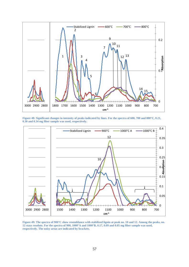
57

Figure 48: Significant changes in intensity of peaks indicated by lines. For the spectra of 600, 700 and 800°C, 0.21,

0.30 and 0.34 mg fiber sample was used, respectively.

Figure 49: The spectra of 900°C show resemblance with stabilized lignin at peak no. 10 and 12. Among the peaks, no.

12 stays resolute. For the spectra of 900, 1000°A and 1000°B, 0.17, 0.09 and 0.05 mg fiber sample was used,

respectively. The noisy areas are indicated by brackets.

280029003000

0

0.1

0.2

700800900100011001200130014001500160017001800

Ab

sorp

tio

n

cm-1

Stabilized Lignin 600°C 700°C 800°C

1 3 4

5

7

9

10 11

12 13

14 15

2

6

280029003000

0

0.05

0.1

0.15

0.2

0.25

0.3

0.35

0.4

700800900100011001200130014001500

Ab

sorp

tio

n

cm-1

Stabilized Lignin 900°C 1000°C A 1000°C B

12

10

58

Figure 50: Peak no. 12 stays resolute. For the spectra of 1100, 1200°, 0.10, 0.11 mg fiber sample was used, respectively.

The noisy areas are indicated by brackets.

To compare the carbonized lignin fibers with commercially available carbon fibers on the

market, a spectrum of PAN-based carbon fibers, from the TORAYCA T1700S brand (Toray

carbon fibers America Inc., Santa Ana, USA), was recorded (Figure 51).

The shoulder peak near 1715 cm-1

is attributed to C=O stretching. The bond is related to the

cyclized structure of PAN and the faint peak indicates that trace amounts are still present in

the carbonized structure of the fibers. (Arbab et al. 2014)

The strong peak at 1640 cm-1

is hard to interpret. But it is probably due to vibrations in water

or aromatic rings (Coates 2000), or even a combination of both. (Recall the problematic and

hydroscopic nature of KBr in section 2.5.1). Another explanation, provided by the literature,

is that the peak is related to stretching of C=N conjugated with C=C (Ju, Xu & Ge 2014).

However, little to no nitrogen amount should be present in the carbonized form. The side

peak, 1540 cm-1

, is accompanied by the stronger peak and is also associated with the aromatic

stretching. (Coates 2000, Solomons, Fryhle 2011b)

The bands at 1460 and 1370 cm-1

are assigned to C-H bending in different modes (Ju, Xu &

Ge 2014, Arbab et al. 2014). 1280 cm-1

can be interpreted as stretching in nitrate compounds

and is in that case coupled with the peak at 1640 cm-1

(Coates 2000). The peak can also be

related to ether bonds. It could be either one since they overlap in the same region (Coates

2000). Nevertheless, the peak aligns nicely with the stabilized lignin spectra in this region and

may therefore be vibrations of C-O bonds in ethers.

280029003000

0

0.05

0.1

0.15

0.2

0.25

700800900100011001200130014001500

Ab

sorp

tio

n

cm-1

Stabilized Lignin 1100°C 1200°C

12

59

The region between 1000 and 1200 cm-1

is a result of stretching in alcohols and aliphatic

ethers (Solomons, Fryhle 2011b). Regardless, the peak at 1068 cm-1

is attributed to C-H

bending (Arbab et al. 2014).

Similarly as lignin, peaks are located around 835 cm-1

in the spectrum. They represent out-of-

plane deformation in C-H bonds in mono or disubstituted aromatic rings (Coates 2000,

Solomons, Fryhle 2011b).

The area between 2800 and 3000 cm-1

are related to stretching vibrations of C-H. .

Figure 51: Spectrum of PAN-based carbon fibers. Interesting peaks are indicated by wavenumber (cm-1). 0.09 mg

sample was used.

0

0.05

0.1

0.15

0.2

0.25

0.3

0.35

7009001100130015001700190021002300250027002900

Ab

sorp

tio

n

cm-1

TORAYCA T1700S

2850

2918

1716

1643

1540

1460 1370

1280

1068

835

60

3.5 SEM SEM enabled high resolution imaging of a few selected fibers. All fibers pictured below were

also analyzed in ESD. For comparison, the light microscopy images from the same batch as

the following fibers are found in appendix 8.2.4.2.

The interaction volume is a couple of micrometers deep into the material from the surface.

3.5.1 Imaging

The aim of the analysis was to inspect the fiber structure prior and after carbonization to

certain temperatures as well as the effect of the heating rate and applied load. The images was

acquisitioned by a backscatter detector, therefore (as mentioned in 2.6) contrasts indicate

different chemical composition.

To compare the carbonized lignin fibers with commercially available carbon fibers, an image

of TORAYCE T1700S (Toray carbon fibers America Inc., Santa Ana, USA), was acquired.

These PAN-derived carbon fibers are presented in Figure 52.

Contamination (bright spots) is clearly visible on the surface. Analysis of the particles is

presented below, in section 3.5.2. Nevertheless, the fibers seem very uniform in shape and

have no visible defects whatsoever.

Figure 52: SEM image of TORAYCE T1700S carbon fibers. The diameters are (upper) 7.07 µm and (lower) 6.99 µm.

In Figure 53 below, the fiber axis and the cross-section of stabilized lignin is pictured. The

intensity from the axial surface is brighter in comparison with T1700S. The higher intensity

might be caused by higher proportions of oxygen in the surface compared to carbon, since O

has a higher atomic number than C. The slightly noisy appearance may be caused by uneven

distribution of different compounds across the surface.

A few contaminants (white dots) are also found, although smaller in size. When handling the

lignin fibers, carbonized as stabilized, they became easily charged with static electricity. As a

consequence they probably attracted small dust particles, hence the contamination seen in the

following images.

61

Figure 53: SEM images of stabilized lignin fibers. Image a) and b) shows the surface of fibers in the axial direction

while c) shows the cross-section. The diameter of the fiber is in a) 50.7 µm b) 55.6 µm and c) 39.9 µm.

The intensity is still very bright after carbonization to 300°C, indicating that the material

changed little in composition (Figure 54).

Protuberance is often seen in the images, for example in Figure 54 and Figure 56 a. It is an

artifact produced in the extrusion and results unfortunately in fibers that are not entirely

uniform in shape.

Figure 54: SEM image of a fiber carbonized at 1 K/min to 300°C. The image shows the surface of fibers in the axial

direction. The smaller diameter (to the left) of the fiber is 41.4 µm while the protuberance (to the right) is 50.3 µm.

The intensity has decreased in the 500°C carbonization sample and the fiber has become

darker (Figure 55). Furthermore, the static seems to have disappeared and the signal from the

surface is more uniform in intensity (excluding contaminating particles).

The cross-section, Figure 55 b, displays a fiber that appears to be very grainy.

a) b)

c)

62

Figure 55: SEM images of fibers carbonized at 1 K/min to 500°C. Image a) shows the surface of fibers in the axial

direction while b) shows the cross-section. The diameter of the fiber is in a) 50.2 µm and b) 50.6 µm.

As the temperature increases to 1000°C we start to see porosities in the fibers (Figure 56). An

extreme case is displayed in Figure 56 a), where the fiber is covered with deep pinholes.

Image b) and c), on the other hand, shows minor distribution of pores across the surfaces.

Figure 56: SEM images of fibers carbonized at 1 K/min to 1000°C. Image a), b) and c) shows the surface of fibers in

the axial direction while d) shows the cross-section. The diameter of the fiber (and bulge in parenthesis) is in a) 39.3

µm (70.0 µm), b) 35.9 µm, c) 37.1 µm (43.4 µm) and d) 37.2 µm.

The pores become more distinguishable when the carbonization temperature reaches 1200°C

(Figure 57). When comparing the heating of 10 and 40 K/min in b) and c), respectively, no

differences are apparent. In contrast, the slowest heating, 1 K/min in a), appears to have

affected the fiber structure the most.

a) b)

a) b)

c) d)

63

Figure 57: SEM images of fibers carbonized at a) 1 K/min, b) 10 K/min and c) 40 K/min to 1200°C. Image a), b) and c)

shows the surface of fibers in the axial direction while d) shows the cross-section. The diameter of the fiber (and bulge

in parenthesis) is in a) 33.0 µm (43.7 µm), b) 30.6 µm (38.5 µm) and c) 42.4 µm.

Next, we evaluate fibers from sample A and B (recall section 3.1.2) in Figure 58. Almost no

pores are found in the fibers which retain a uniform shape and composition. The cross-section

c) hints of a slightly bright circle in the periphery. This might indicate a skin-core formation

that contains more oxygen than the interior.

a) b)

c)

64

Figure 58: SEM images of fibers carbonized at 10 K/min to 1000°C under increasing load from 10 mN to 300 mN

between 375-975°C in a) and to 400 mN between 350-950°C in b) and c). Image a) and b) shows the surface of fibers

from sample A respectively B in the axial direction while c) shows the cross-section of a fiber from sample B. The

diameter of the fiber is in a) 26.6 µm, b) 36.4 µm (left) 37.1 µm (right) and c) 26.8 µm.

3.5.2 Energy-dispersive X-ray spectroscopy

The EDS-scan was performed over three areas:

The fiber axis, rectangle Figure 59 a).

The whole cross-section, circle in Figure 59 b).

The inner section of the cross-section, square in Figure 59 b).

Figure 59: a) The scanned area along the fiber axis is indicated by the rectangle. b) The circle indicates the scan over

the whole cross-section and the square the inner section. The fiber in a) and b) is the same as in b) resp. c) in Figure

56.

a) b)

c)

a) b)

65

In this fashion, spectra were gathered from all fibers pictured in the previous section 3.5.1 and

some that were purely for the EDS-study. A few examples of spectra are found in Figure 60,

which were collected from the fibers in Figure 56.

Figure 60: EDS-spectra generated from the scanned areas above, Figure 59, showing Kα-energies from emission in

various elements in the fiber. Spectrum 8 belongs to the axial scan, spectrum 36 to the cross-sectional area and

spectrum 37 the inner section.

The main elements found in the fibers were carbon, oxygen and sulfur. The O and C relate to

the lignin molecule itself, whereas S residues are remains from the kraft pulping process

(section 1.2.3.1).

In some instances, trace amount of inorganic species, among silicon, alumina, chlorine and

potassium (rare), was also identified, which rarely exceeded 0.5 wt%. The Al originates

probably from alumina foil that was used to protect and store lignin fibers, i.e. foil was

wrapped around the fibers. The K and Cl are probably constituents in salts and are not part of

the lignin molecule. The salts could originate from the skin when handling the fibers, but this

is highly speculative.

66

X-ray analysis of the particles that cover the surface of the PAN-derived carbon fibers in

Figure 52 shows that main constituents are potassium and chlorine. Without any doubt the

particles are composed of potassium chloride (KCl) crystals.

Elemental analysis of the contaminant on the cross-section in Figure 58 shows a large variety

of elements, among Si, Al, Ca and Na.

From the spectral analysis along the fiber axis, the average elemental composition of the

fibers, sorted by carbonization temperature, was put into the chart seen in Figure 61. The

proportion of oxygen is observed to decrease with carbonization temperature. Meanwhile, the

relative carbon content increases passively. Note that the amounts of carbon do not increase

during the carbonization but rather increase proportionally to the entire content. This means

that the majority of the carbon structure stays resolute to temperature changes whereas

unstable, weakly bonded or volatile compounds are eliminated from the polymer

macromolecules and evaporate. Oxygen containing compounds are likely to disappear from

the fiber.

The relative sulfur content changed little during the carbonization and may indicate that the S

atoms are strongly attached to the polymer macromolecule with covalent bonds.

In order to be classified as carbon fibers, the amount of carbon must at least be 90 wt%

(section 1.2). The lignin carbon fibers do not quite reach the bar. On the other hand, the PAN-

derived carbon fibers barely meet the criterion themselves. The chemical composition is

specified to 93 % in the datasheet of T1700S. According to the analysis of the atomic weight

this appears to be true.

67

Figure 61: Relative content of carbon (blue), oxygen (red), and sulfur (green) after carbonization is indicated as a) the

weight percentage (Wt %) and b) atomic percentage (At %).

Data from compositional analysis of the cross-sections is gathered in Figure 62. For all

carbonization states we observe that the carbon content is greater in the interior of the fibers,

followed by slightly less in the whole cross-section. The conclusion is that the oxygen is

generally higher on the edges or in the periphery of the fiber cross-section. In all instances the

0

10

20

30

40

50

60

70

80

90

100

StabilizedLignin

300°C 500°C 1000°C 1200°C TORAYCAT1700S

Wt

%

C O S

a)

0

10

20

30

40

50

60

70

80

90

100

StabilizedLignin

300°C 500°C 1000°C 1200°C TORAYCAT1700S

At

%

C O S

b)

68

highest amount of oxygen is found on the fiber axis surface along with the lowest amount of

carbon.

The amount of carbon in the interior of the 1000°C carbonized fibers actually meets the

requirement of 90 wt% carbon.

Figure 62: Relative content of carbon (blue), oxygen (red), and sulfur (green). The full colored pile represents the

composition of the axial surface of the fiber, horizontally striped piles the cross-section and diagonally dashed piles

the inner square.

Compositional analysis was also carried out for the fibers carbonized under increasing force

(Figure 63). Although the fiber of sample B contains slightly more carbon than the fiber of

sample A, the content is essentially the same for both. The level at the axis surface is however

higher, in both cases, than that of fibers carbonized under static load. The interior carbon

content is noticeable, a few percent, higher as well.

The fiber of sample B fulfills the 90 wt% carbon requirement in all aspects.

0

10

20

30

40

50

60

70

80

90

100

Stabilized Lignin 500°C 1000°C

Wt

%

C O S Axial Cross-section Inner Square

69

Figure 63: Relative content of carbon (blue), oxygen (red), and sulfur (green) in lignin fibers carbonized under

increasing load.

3.6 Light Microscopy The lignin fibers were studied in microscope in order to observe the degradation and

structural change that took place during carbonization. The structural integrity of the surface

correlates to strength. So any information regarding defects would for instance explain

premature rupture in tensile tests (i.e. low tensile strength) or even in the TMA-carbonization

itself. A newer series can be found appendix 8.2.4.1.

If not stated otherwise all images were taken with a magnification of x50 with focus adjusted

to the top of the fiber. However, since the microscope was configured with an improper

calibration when measuring the fibers, the scales indicated in the images are somewhat

misleading. In reality the length, represented by the scale, should be about 20-25 µm less than

indicated (estimated from the newer series).

Nevertheless, the same incorrect calibration and resolution was used for all measurements and

images, hence the diameter differences between carbonized and stabilized lignin fiber could

be calculated (Table 7)

When evaluating the images, the surface of the stabilized fibers is moderately glossy and

reflects plenty of light that is incident from above. The fibers also appear grainy but the

surface is still smooth (Figure 64).

0

10

20

30

40

50

60

70

80

90

100

A Axial B Axial B Outer Cross-section

B Inner Square Axial 1000°C

Wt

%

C O S

70

Figure 64: Individual stabilized lignin fibers. The magnification in the image to the right is x20.

The appearance is maintained during carbonization up to 500-600°C where small cavities or

craters start to form (Figure 65 and Figure 66). The craters gradually increase in amount and

at 800-900°C they overwhelm the surface which seems porous and rough at this point (Figure

67 and Figure 68). Although plenty in number, the craters do not appear to be very deep. The

fibers also lose the glossy appearance and reflect less light, in other words they become

darker.

Figure 65: Individual lignin carbon fibers carbonized to 500°C.

Figure 66: Individual lignin carbon fibers carbonized to 600°C.

100 µm 300 µm

100 µm

100 µm 100 µm

100 µm 100 µm

71

Figure 67: Individual lignin carbon fibers carbonized to 800°C.

Figure 68: Individual lignin carbon fibers carbonized to 900°C.

At 1000°C and onward the contrast of the fibers is extremely dark (Figure 69, Figure 70 and

Figure 71). The craters are still present, although larger in diameter.

Figure 69: Individual lignin carbon fibers carbonized to 1000°C.

100 µm 100 µm

100 µm 100 µm

100 µm 100 µm

72

Figure 70: Individual lignin carbon fibers carbonized to 1100°C.

Figure 71: Individual lignin carbon fibers carbonized to 1200°C.

An explanation for the crater formations may be that the surface reacts with something during

the carbonization which causes gouging. For example, presence of oxygen in the TMA-

system or contamination of particles on the fiber surface.

Never the less, the size of the fiber deteriorates with increasing temperature (Table 7). At first

the diameter remains principally the same. After 500°C the change is starting to get

noticeable.

If compared with the values that were calculated from the TGA-measurements, the change in

percent roughly match each other, give or take a few units (Figure 42; Red triangles).

100 µm 100 µm

100 µm 100 µm

73

Table 7: Displaying average diameters of stabilized respectively carbonized lignin fibers, sample standard deviation

and number of samples used in the measurements. The percentage relate to the remaining diameter after

carbonization. Since the microscope was not correctly calibrated during the diameter measurement of the fibers

carbonized to 400, 500 and 1000°C, the data for those are not displayed. However, the same, yet wrong, calibration

was used thus the residual diameter could be calculated.

Temperature (°C)

Heating (K/min)

Average Diameter (µm)

Sample Standard Deviation (µm)

Residual Diameter

(%)

Data Points

Stabilized Lignin

0 47.1 5.91 100 30

300 10 46.6 5.35 99.0 30

400 1 N/A N/A 95.1 6

500 1 N/A N/A 93.4 3

600 10 39.8 3.47 84.5 29

900 10 38.1 4.91 80.9 29

1000 1 N/A N/A 75.8 14

74

4 Discussion Previous results, interesting aspects of the future, importance in broad sense and ethics are

discussed in this section.

4.1 Analysis of the main results The results are discussed in detail in each topic, ordered after method and analysis.

4.1.1 TMA

The TMA measurement of the carbonization shows that the fiber deformation is only

temperature dependent. Different heating rates, at least for values between 1 and 40 K/min, do

not seem to affect the deformation pattern (Figure 24). The deformation per temperature

neither increases nor decreases when varying the rate of heating.

The deformation occurs in three steps as shown by the curve in Figure 21. The extension

coefficient α curve indicates maximum deformation at 375, 530 and 650°C. Analogous to the

TGA measurement the loss of mass also occur in three steps, where the derivative maximums

are found at 425, 560 and 785°C (Figure 41).

Variations of the deformation were observed (Figure 23). Samples with 50 fibers tended to

follow the same pattern whereas samples with fewer fibers did not. Logically, the samples

with fewer fibers would contract less compared to the samples with higher amount, due to the

static force exerted on the fibers. Small variations are possible since lignin fibers are

amorphous, but these strong variations have other explanations. The behavior could for

instance be attributed to mounting and/or sample preparation.

Furthermore, the deformation comes to a standstill above 1000°C. Probably a sign that the

fiber is fully carbonized, meaning that remaining molecular compounds in the fiber are stable

enough to withstand the temperature (i.e. further evaporation of volatile substances and

compounds will not occur) and that the structure of the lignin polymers is sufficiently cross-

linked and has retained a strong conformation that takes up as little space as possible (i.e. the

fiber will not contract more), preferable aromatic in nature.

4.1.2 Dia-Stron

The overall stability of the carbonized lignin fibers is by this assumption stronger than the

non-carbonized lignin fiber. The Dia-Stron results support this by showing the improved

mechanical properties of the fibers. Compare the E-modulus and tensile strength (around 36

GPA, and 600 MPa, respectively) of fibers that underwent carbonization to 1000°C to the E-

modulus and tensile strength (around 5 GPa and 150 MPa, respectively) of the stabilized

lignin fibers.

Along with deformation, the rate of heating did not affect the mechanical strength properties

either. The E-modulus and tensile strength remained principally the same for all rates,

although 1 K/min were slightly better. Since rate did not matter much, the carbonization rate

was chosen to 10 K/min for practical production of samples to, for instance, the Dia-Stron and

FTIR-spectroscopy. A carbonization to 1000°C at 1 K/min would take approximatively 16

hours whereas a 10 K/min carbonization would take only 2 hours (including cooling).

75

When the load was increased to compensate for the contraction, the carbonized lignin fibers

showed result of improved E-modulus, they became stiffer in other words. Compared to the

average value for carbonization under static load, 36 GPa, the E-modulus reached values

around 50 GPa. As for the tensile strength, the change was too insignificant to be considered

an improvement.

Depending on the force and interval, where the load was applied, the stiffness of the carbon

fibers could be adjusted (Table 5). Not necessarily did higher loads mean higher E-modulus.

On the contrary, fibers that had been applied an slowly increasing force over a long interval

(300-900°C) to a high final load had approximatively the same E-modulus as fibers that had

been applied a rapidly increasing force over a small interval (400-600°C) to a low final load

(Compare sample G & H against E & F, Table 5).

By studying the deformation, fibers that had contracted least showed better E-modulus than

those who had contracted more. The best result was achieved for fibers that stayed at positive

length during the entire carbonization (above 0% in Figure 27). It seems that the restriction of

the fiber contraction during the carbonization has a larger impact rather than the force itself.

In this regard, the ramping of force was preferable started early in the carbonization (around

300°C) where the fibers still underwent expansion and were susceptible to load. This

compensated for the tendency to contract early on and resulted in a lower final contraction.

Another way to regulate the contraction was to successively increase the force elevation in

steps as soon as the fibers tended to contract (Figure 30).

It may even be of interest to test applied load as early as the stabilization, since some sintering

takes place there as well.

Regarding the load, the fibers were very sensitive to increasing stress during the

carbonization. Many TMA carbonizations failed due to this. Figure 30 shows two examples.

The E-modulus of those fibers that ruptured mid carbonization was essentially the same as

that of fibers that had been carbonized under low static force. Low rates of increasing force

are therefore necessary.

The following discussion regarding improved mechanical properties is only speculative from

my behalf. The improved stiffness may be attributed to increased alignment of the lignin

polymer aromatic chains. Initially the lignin polymers are somewhat randomly distributed in

the fiber, i.e. the order is random and the fiber is considered amorphous. However, it is not

excluded that some molecular orientation may be present. During the carbonization,

aromatization or cyclization of the polymer chains is thought to occur and due to the random

organization the resulting carbon fiber will achieve turbostratic ordering.(Beste 2014) By

instead applying an increasing load on the fibers in the process, the polymers are forced into a

more aligned structure as they react and undergo conformational changes, facilitating cross-

linking and aromatization along the direction of the fiber axis. Compare with a tangled metal

chain that unfolds and becomes straightened as you pull it in both ends. The fibers are

probably still turbostratic although to a less extent.

76

In comparison, graphitic and ordered MPP has generally higher E-modulus compared to the

turbostratic PAN (Liu, Kumar 2012, Huang 2009). This suggests that the lignin carbon fibers

have obtained a conformation that is similar to graphitic.

Under almost negligible force, the fibers contract unhindered during carbonization, mainly

due to the conformational rearrangement that occurs intra- and intermolecularly in the

polymer molecule structure and polymer network, respectively. Participating in the

rearrangement are free-radical, cross-linking, condensation, cyclization and aromatization

reactions. The molecular structure becomes more tightly bonded and more stable in every

direction, i.e. in and between polymers constituting the fibers (Figure 72 a).

By increasing the load successively the fiber contraction is hindered. The applied load in the

direction of the fiber axis straightens out the polymer chains, facilitating the forming of

favorable conformations along the chains and the fiber axis whereas adjacent conformational

reactions are unfavorable and thus inhibited by the force (Figure 72 b).

Figure 72: Simple depiction of the intramolecular conformational changes. Thick lines represent polymer chains while

thin lines represent molecular structures (e.g. cross-links, conjugated aromatic and cyclic structures, aliphatic ethers

etc.) that form during carbonization and bind the chain together into a new conformation. In a) conformational

reactions occur freely in every direction whereas in b), the reactions are only favored in the direction of the force. In

reality one has to account for the random ordering and branching of the polymers as well as the entire polymer

network.

Another theory is that the force breaks apart weak structures during the carbonization. The

strongest remain while the broken structures, which cannot undergo further cross-linking,

simply decompose by the heat and evaporate.

4.1.3 TGA

Without any doubt partial combustion occurred during the TGA measurement of the

carbonization at Innventia AB. Since combustion is caused by oxidation reactions that take

place within the fiber the mass temporarily increases slightly (oxygen react and form

temporary intermediates). This can be observed as a convex shape or bulge in the curve

between 450 and 720°C in Figure 40, where the mass still decrease although slightly less.

(Vaimakis 2013)

4.1.4 FTIR

The FTIR-study proved to be quite difficult to implement, since carbon fibers are in general a

material with high absorption. Even a little amount of carbon fiber resulted in low

transmittance.

a) b) Force

77

In order to work around this problem, extremely small amounts of sample were used in this

study. In contrast to the normal ratio of 3 mg sample per 300 mg KBr in the pellet,

approximatively a tenth of the recommended sample amount was used. Implications resulting

from this were that the signal became indistinguishable from noise at some frequencies and

the intensity of water became dominant in the spectra, especially at higher degree of

carbonization (i.e. higher carbonization temperature) where even lower amounts were used.

The peak at 1600 cm-1

, attributed to aromatic skeleton, became masked by the dominant

intensity of water around 1640 cm-1

in this respect. (Most likely water, since a broad band

with large intensity was found at 3100-3700 cm-1

in all spectra.)

According the literature, main compounds released during the carbonization are CH4, water,

CO2 and CH3OH. (Li et al. 2013) Mainly oxygen containing compounds are released during

the carbonization. Water is probably released in the early stage of carbonization, accounting

for the largest loss of mass.

The carbonization involves dehydrogenation and decarboxylation reactions in combination

with condensation and aromatization, releasing nearly all non-carbon elements (Chatterjee et

al. 2014). Other weakly bonded side groups of the lignin polymer is probably eliminated

through homolysis and evaporated during the carbonization.

Homolytic cleavage of linkages constituting the polymer chain also occurs, resulting in

radical formations that allow for rearrangement of the lignin molecule conformation. For

instance, the most commonly and also one of the weakest linkages, the β-O-4 linkage is likely

involved in the radical reactions. (Beste 2014)

Furthermore, oxygen containing functional groups and linkages in lignin may supposedly

facilitate cyclization steps that transform weak ether and rotatable aliphatic linkages into

stable and stiff aromatic units. (Beste 2014)

In the FTIR series from 300 to 1200°C, nearly all features characteristic to lignin vanished as

the carbonization temperature increased. Although many compounds dissociated from the

originally stabilized lignin, some compounds endured the temperature changes and was

removed slower than other.

The decarboxylation and release of CO2 is indicated by the fast decreasing intensity of 1710

cm-1

between 300°C and 500°C (Peak 1 Figure 47) (Huang, Ma & Zhao 2015). As indicated

by the reduced bands at 1365-1370, 1210-1220, 1080 and 1030-1035 cm-1

, phenolic hydroxyl,

hydroxymethyl and ordinary hydroxyl groups were consumed in condensation reactions

during the early carbonization (Peak 1 Figure 47), contributing to release of water and ether

formation. The increasing absorbance intensity of 1080 cm-1

, attributed to aliphatic ethers

(Peak 12 Figure 49-Figure 50), demonstrates that ether structures increase after 900°C,

connecting aromatic rings together. (Huang, Ma & Zhao 2015) Some ether bond probably

originated from linkages (β-O-4 and 4-O-5 for instance), which may be the reason that the

intensity never faded out in the region. (Beste 2014)

78

Another spectral feature that remained after full carbonization to 1000°C, was in-plane

deformation of C-H in guaiacyl rings at 1150 cm-1

and 1030-1035 cm-1

(Peak 10 and 13 in

Figure 47-Figure 50). The aromatic structure is thought to remain and even increase during

the carbonization and the result points in this direction. Peak 10 and 13 actually increases in

absorbance after 900°C.

However, other results points in the opposite direction. The intensity of the band regions at

1515 cm-1

and 1430 cm-1

, attributed to breathing of aromatic rings with contribution of in-

plane deformation of C-H in the latter, decreased (Peak 3 and 5, respectively, in Figure 47-

Figure 50). The first band decreased faster than the second until it had disappeared completely

at 600°C whereas the second band still remained, but may be attributed to noise, after 600°C.

As for the peak at 1600 cm-1

, also attributed to breathing of aromatic rings, it is concealed

under the dominant water intensity in the region and thus cannot be fully evaluated.

4.1.5 SEM

The EDS analysis along with FTIR confirms the fact many that oxygen containing

compounds dissociate and disappear though evaporation during carbonization, as indicated by

the decreasing amount of oxygen.

SEM imaging shows that the fibers darken during the carbonization. Pinholes formations

appear at high carbonization temperature which may be the same formations shown in the

light microscope imaging.

The surface of the fibers seems oxygen rich in content, as indicated by comparisons between

inner cross-sections and edges/surfaces (Figure 62). Skin-core structures are therefore most

likely present in the fibers which was stated in the literature (section 1.2.3.3).

4.1.6 Microscopy

Defects and the seemingly porous surface probably weakened the carbonized lignin fibers.

The wide spread in the tensile strength graphs are most likely a testament to this (Figure 37).

According the literature pores and defects could arise from elimination of heteroatoms

(section 1.2.3.3). In our case the SEM-study imply that the fiber surface is rich in oxygen

content which would explain the porous appearance after carbonization.

4.2 Impact in a broad sense The performance of lignin carbon fibers is not nearly close to that of commercially available

carbon fibers. In the sense of progress towards obtaining carbon fibers of lignin suitable for

the industrial use, a long way still remains.

However, the improved mechanical performance that was achieved and presented, in this

work, for stabilized lignin fibers that underwent carbonization under increasing load is a step

in the right direction. The information is beneficial regarding future work in discovering

better parameters in order to improve the mechanical strengths. In that aspect, this work

would serve as a starting point.

In the sole purpose of the project, the carbonization was focused on small scale production

where a few fibers were carbonized at a time. In mass-production, however, where large

79

quantities of fibers are carbonized, one has to consider that the heat and energy needs to be

high enough for carbonization to take place. The speed of the carbonization is also of great

importance.

The information regarding heating rate is therefore of value in industrial applications. As

indicated, the rate of heating does not matter considerably for the mechanical strength

properties. If one wants to produce large quantities of carbon fibers from lignin, the speed of

the process is only limited by heating rate and carbonization temperature, meaning that the

process can be made as fast as the heating allows for.

When and if the problems of the production of lignin carbon fibers are solved, the prices of

carbon fiber will plummet, since there is an abundance of lignin in the pulping process. In this

case strong reinforced carbon fiber composites could be manufactured cheaply and would, for

instance, greatly benefit production of low weight vehicles which in turn would lower the fuel

consumption, where economical resources can be saved. Lower fuel consumption would also

lead to a healthier ecological environment. Needless to say, the transport industry would

greatly benefit from this.

4.3 Ethical implications in a broad sense As mentioned above, carbon fiber production from lignin would have a lot of positive

consequences. However, and this is highly speculative from my part, the demand of low cost

carbon fibers would most likely increase as a result. In that case one has to consider the risk of

increased deforestation in order to supply with lignin for carbon fiber production. Even

though lignin is considered a by-product today, it may be the main product from wood

tomorrow.

In the worst case scenario, the pulping process would be so focused on extracting lignin that

the other components, e.g. for paper production, would simply be disregarded as waste. The

tables would have been turned. The full potential of wood would not be utilized and a lot of

resources would go to waste.

Deforestation affects the nature and ecological systems. The topic is always under debate,

especially when talking about the rainforests.

The ever increasing use of tablets, smartphones etc. in today’s society, will render

newspapers, books, papers etc. obsolete in the near future. The trend will probably cause the

production of paper materials to decrease by the looks of it. Therefore it would be imperative

to find another uses for the pulping process. If lignin carbon fibers can be improved, it would

solve the problem.

4.4 Future perspectives

More research must be put into improving the mechanical performance of lignin carbon

fibers. In order to do so, the carbonization process must be fully understood. Today, little

information is known about the chemical reactions and conformational rearrangements that

take place which would be an interesting aspect to study in future research. The FTIR study in

this work did not fully answer the questions.

80

Further testing of load is another interesting aspect. The force program must be optimized so

that unnecessary rupture of the fibers is inhibited. In addition, large expansion of the fibers is

something to consider in respect to how the mechanical performance would be affected.

Moreover, it would be interesting to experiment with different loads during the stabilization

as well.

81

5 Conclusion The main goal of the project was to optimize the carbonization process (compare section 8.1.2

and 1.1) and to obtain carbon fibers with good mechanical properties. Recommendations for

the parameters of interest are as follows:

Since the rate of temperature elevation did not affect the strength properties

considerably much, i.e. changing the rate neither improved nor impaired the

mechanical strength, any rate can be selected solely in the purpose and suitability of

the production. In this work 10 K/min proved useful but an increased rate would

benefit faster carbon fiber production from stabilized lignin. However, 1 K/min may

be to slow and may induce defects in the carbon fibers as seen in the light microscopy

and SEM imaging. For small scale production 10 K/min is recommended.

Regarding carbonization temperature, the E-modulus and tensile strength reached its

maximum around 1000°C. The fiber contraction also stopped at that temperature.

Carbonization to higher temperatures is possible, but there is a risk that the fibers may

become severely damaged, especially at the surface, affecting the tensile strength. A

temperature around 1000°C is therefore recommended.

The E-modulus was affected considerably by applying an increasing load during the

carbonization, which hindered the contraction of the fibers. When the dimensional

change was close to 0 % the carbonized lignin fibers had and E-modulus of about 50

GPa, an improvement of 14 units from 36 GPa. The recommendation here is to apply a

force early in the carbonization process that inhibits the contraction as much as

possible. For instance, from 0.01 to 0.35 N between 300 and 900°C, for approximately

5 fibers.

Although the mechanical strength was improved, the lignin carbon fibers are still not suitable

for industrial use. The improvement is however a step in the right direction and would serve

as a guideline for further load testing during carbonization. Nevertheless, these

recommendations should optimize the production of lignin carbon fibers regardless of

mechanical strength. In sense of optimization, the goal was achieved!

The EDS analysis revealed that much oxygen was removed from the lignin during the

carbonization process. The FTIR analysis supported this by showing that several oxygen

containing compounds were driven out by the heat. The formation of aromatic structure was

however difficult to observe because peaks, representing aromatic structures, were masked by

the dominant water intensity in the FTIR spectra.

The SEM in combination with the EDS showed the presence of skin-core structures in the

fibers. Furthermore, defects like “porous surface” were observed in the SEM and light

microscopy imaging. These irregularities affected the tensile strength of the fibers.

82

6 Acknowledgements This work was carried out in the Lignin Carbon Fiber group at Innventia AB under

supervision of Professor Lennart Salmén.

I wish to express my sincere gratitude to Professor Lennart Salmén for introducing me to the

area of research regarding lignin and carbon fibers and also allowing me to work with this

project. His door was always open throughout the project and in dire need he would always

provide with advices and suggestions.

I would also like to thank Anne-Mari Olsson for introducing me to the practical work at the

start of the project, helping me solve the “mysteries” of the TMA-instrument and showing me

how to operate the TGA. Whenever there was a practical or technical issue regarding

equipment or preparations, she always had a solution at hand.

I was able to operate the FTIR-equipment at Innventia AB thanks to Jasna Stevanic-Srndovic

and her instructions.

My gratitude also goes to Joanna Hornatowska who always was kind and considerate. She

helped me with the SEM-study. And thanks to her instructions I could fully utilize the light

microscope.

Many thanks to the members of the Lignin Carbon Fiber group for your support. I hope this

work will contribute in your further work with lignin carbon fibers.

I would like to thank Mårten Åkerström for “serving me”, as he himself would put it, in

solving the adhesive problems, ordering graphitic components (adhesive and plates) and

providing me with stabilized lignin fibers. Thank you for meaningful discussions.

Thanks to Anders Uhlin for showing me how to perform the stabilization on my own when all

stabilized lignin fibers were consumed.

To Dr. Thomas Edert and Daniel Aili, at Linköping University, I wish to express my

appreciation that you accepted the role of being examiner and internal supervisor for this

thesis. Your suggestions and advices are greatly acknowledged.

At last, but not least, I would like to thank my family for providing support and temporary

accommodation during the difficult time of train service in Sweden. I always think about you

and appreciate you even though it may not seem like that sometimes.

83

7 References

Abo, H. 2010, The ABSs of Measurement Methods: KBr Pellet Method, vol. 14 edn, FTIR

Talk Letter, Shimadzu Corp.

Agarwal, U.P., McSweeny, J.D. & Ralph, S.A. 2011, "FT-Raman Investigation of Milled-

Wood Lignins: Softwood, Hardwood, and Chemically Modified Black Spruce Lignins",

Journal of Wood Chemistry & Technology, vol. 31, no. 4, pp. 324.

Arbab, S., Mirbaha, H., Zeinolebadi, A. & Nourpanah, P. 2014, "Indicators for evaluation of

progress in thermal stabilization reactions of polyacrylonitrile fibers", Journal of Applied

Polymer Science, vol. 131, no. 11, pp. n/a.

Bajaj, P., Sreekumar, T.V. & Sen, K. 2001, "Effect of reaction medium on radical

copolymerization of acrylonitrile with vinyl acids", Journal of Applied Polymer Science,

vol. 79, no. 9, pp. 1640-1652.

Baker, D.A. & Rials, T.G. 2013, "Recent advances in low-cost carbon fiber manufacture from

lignin", Journal of Applied Polymer Science, vol. 130, no. 2, pp. 713-728.

Becker, W.M. 2008, The world of the cell, 7th edn, Pearson, Benjamin Cummings, San

Francisco.

Beste, A. 2014, "ReaxFF Study of the Oxidation of Lignin Model Compounds for the Most

Common Linkages in Softwood in View of Carbon Fiber Production", Journal of

Physical Chemistry A, vol. 118, no. 5, pp. 803-814.

Boccara, A.C., Fournier, D., Kumar, A. & Pandey, G.C. 1997, "Nondestructive evaluation of

carbon fiber by mirage-FTIR spectroscopy", Journal of Applied Polymer Science, vol.

63, no. 13, pp. 1785-1791.

Braun, J.L., Holtman, K.M. & Kadla, J.F. 2005, "Lignin-based carbon fibers: Oxidative

thermostabilization of kraft lignin", Carbon, vol. 43, no. 2, pp. 385-394.

Brodin, I., Gellerstedt, G., Sjöholm, E. & Ernstsson, M. 2012, "Oxidative stabilisation of kraft

lignin for carbon fibre production", Holzforschung, vol. 66, no. 2, pp. 141-147.

Brodin, I., Sjöholm, E. & Gellerstedt, G. 2010, "The behavior of kraft lignin during thermal

treatment", Journal of Analytical and Applied Pyrolysis, vol. 87, pp. 70-77.

Brown, M.E. 2001, Introduction to thermal analysis. [Elektronisk resurs] techniques and

applications, 2nd edn, Kluwer Academic, Dordrecht ; London.

Chatterjee, S., Johs, A., Jones, E.B., Rios, O., Clingenpeel, A.C., McKenna, A.M., McNutt,

N.W. & Keffer, D.J. 2014, "Conversion of lignin precursors to carbon fibers with

nanoscale graphitic domains", ACS Sustainable Chemistry and Engineering, vol. 2, no. 8,

pp. 2002-2010.

Coates, J. 2000, "Interpretation of Infrared Spectra, A Practical Approach" in Encyclopedia of

Analytical Chemistry, ed. R.A. Meyers, John Wiley & Sons Ltd., Chichester, pp. 10815.

84

Coats, A.W. & Redfern, J.P. 1963, "Thermogravimetric analysis. A review", Analyst, vol. 88,

no. 1053, pp. 906.

Davis, J.R. 2004, Tensile testing. [Elektronisk resurs], Materials Park, Ohio : ASM

International, 2004; 2nd ed.

Derkacheva, O. & Sukhov, D. 2008, "Investigation of lignins by FTIR spectroscopy",

Macromolecular Symposia, vol. 265, no. 1, pp. 61-68.

Egerton, R.F. 2005, Physical principles of electron microscopy. [Elektronisk resurs] : an

introduction to TEM, SEM, and AEM, New York, N.Y. : Springer, c2005.

Faix, O. 1991, "Classification of Lignins from Different Botanical Origins by FT-IR

Spectroscopy", Holzforschung: International Journal of the Biology, Chemistry, Physics,

& Technology of Wood, vol. 45, pp. 21.

Freudenberg, K. 1959, "Biosynthesis and Constitution of Lignin", Nature, vol. 183, no. 4669,

pp. 1152.

Gellerstedt, G., Ek, M. & Henriksson, G. 2009, , Wood Chemistry and Wood Biotechnology.

Heber S., A., João V.F., L., Regina P.W., P., Maria, B.O., Fábio A., A. & Kelysson F., A.

2009, "A supramolecular proposal of lignin structure and its relation with the wood

properties", Anais da Academia Brasileira de Ciências, , no. 1, pp. 137.

Helander, M., Theliander, H., Lawoko, M., Henriksson, G., Zhang, L. & Lindström, M.E.

2013, "Fractionation of technical lignin: Molecular mass and pH effects", BioResources,

vol. 8, no. 2, pp. 2270-2282.

Hergert, H.L. 1960, "Infrared spectra of lignin and related compounds. II. Conifer lignin and

model compounds", Journal of Organic Chemistry, vol. 25, no. 3, pp. 405-413.

HowStuffWorks 2001, 2001-03-21-last update, What is the difference between a hardwood

and a softwood? [Homepage of HowStuffWorks], [Online]. Available:

http://science.howstuffworks.com/life/genetic/question598.htm [2014, 10/31].

Huang, X. 2009, "Fabrication and Properties of Carbon Fibers", Materials, vol. 2, no. 4, pp.

2369.

Huang, Y., Ma, E. & Zhao, G. 2015, "Thermal and structure analysis on reaction mechanisms

during the preparation of activated carbon fibers by KOH activation from liquefied

wood-based fibers", Industrial Crops & Products, vol. 69, pp. 447-455.

Ju, A., Xu, H. & Ge, M. 2014, "Preparation and thermal properties of poly[acrylonitrile- co-(

ß-methylhydrogen itaconate)] used as carbon fiber precursor", Journal of Thermal

Analysis & Calorimetry, vol. 115, no. 2, pp. 1037-1047.

Karmanov, A.P. & Derkacheva, O.Y. 2013, "Application of fourier transform infrared

spectroscopy for the study of lignins of herbaceous plants", Russian Journal of

Bioorganic Chemistry, vol. 39, no. 7, pp. 677-685.

85

Kubo, S., Ishikawa, N., Uraki, Y. & and Sano, Y. 1997, "Preparation of Lignin Fibers from

Softwood Acetic Acid Lignin. Relationship between Fusability and the Chemical

Structure of Lignin", Mokuzai Gakkaishi, vol. 43, no. 8, pp. 655-662.

Kubo, S. & Kadla, J.F. 2005, "Hydrogen bonding in lignin: A fourier transform infrared

model compound study", Biomacromolecules, vol. 6, no. 5, pp. 2815-2821.

Li, Y., Cui, D., Tong, Y. & Xu, L. 2013, "Study on structure and thermal stability properties

of lignin during thermostabilization and carbonization", International journal of

biological macromolecules, vol. 62, pp. 663-669.

Lin, J., Koda, K., Uraki, Y., Kubo, S., Yamada, T. & Enoki, M. 2014, "Improvement of

mechanical properties of softwood lignin-based carbon fibers", Journal of Wood

Chemistry and Technology, vol. 34, no. 2, pp. 111-121.

Liu, Y. & Kumar, S. 2012, "Recent Progress in Fabrication, Structure, and Properties of

Carbon Fibers", Polymer Reviews, vol. 52, no. 3, pp. 234-258.

Lü, Y., Wu, D., Zha, Q., Liü, L. & Yang, C. 1998, "Skin-core structure in mesophase pitch-

based carbon fibers: causes and prevention", Carbon, vol. 36, no. 12, pp. 1719.

Matsumoto, T. 1985, "Mesophase pitch and its carbon fibers", Pure & Applied Chemistry,

vol. 57, no. 11, pp. 1553.

Matsumoto, T. & Mochida, I. 1992, "A structural study on oxidative stabilization of

mesophase pitch fibers derived from coaltar", Carbon, vol. 30, pp. 1041-1046.

McCrum, N.G., Bucknall, C.B. & Buckley, C.P. 1997, Principles of polymer engineering,

Oxford : Oxford Univ. Press, 1997; 2. ed.

Mongeau, R. & Brooks, S.P.J. 2001, "Chemistry and Analysis of Lignin", Food Science and

Technology -New York-Marcel Dekker-, , no. 113, pp. 321-374.

Norberg, I. 2012, Carbon Fibres from Kraft Lignin, KTH Royal Institute of Technology,

Stockholm.

Norberg, I., Nordstrom, Y., Drougge, R., Gellerstedt, G. & Sjo¨holm, E. 2013, "A new

method for stabilizing softwood kraft lignin fibers for carbon fiber production", Journal

of Applied Polymer Science, vol. 128, no. 6, pp. 3824-3830.

Pandey, K.K. 1999, "A Study of Chemical Structure of Soft and Hardwood and Wood

Polymers by FTIR Spectroscopy", Journal of Applied Polymer Science, vol. 71, no. 12,

pp. 1969-1975.

Sjöström, E. 1993, Wood chemistry: fundamentals and applications, Academic Press, Inc, San

Diego.

Solomons, T.W.G. & Fryhle, C.B. 2011a, Organic chemistry, Hoboken, N.J. : Wiley ;

Chichester : John Wiley distributor, cop. 2011; 10. ed., International student version.

86

Steed, J.W., Turner, D.R. & Wallace, K.J. 2007, Core concepts in supramolecular chemistry

and nanochemistry [Elektronisk resurs] / Jonathan W. Steed, David R. Turner, Karl J.

Wallace, Chichester : John Wiley, c2007.

Vaimakis, T.C. 2013, Thermogravimetry (TG) or Thermogravimetric Analysis (TGA),

Introduction edn, Summer School for Thermal Analysis Techniques, Faculty of Science,

Aristotle University of Thessaloniki.

van der Maas, J. H. & Tolk, A. 1962, "The influence of moisture on potassium bromide disks

used in infrared spectrometry", Spectrochimica Acta, vol. 18, no. 2, pp. 235-240.

87

8 Appendix Process, calibrations, calculations and data that may or may not be interesting regarding the

outcome of the project are presented here.

8.1 Process A planning report was established in the beginning of the project. Its purpose was to describe

the project, formulate problems, suggest solution methods and served as a guide for the student during

the project.

Timetable and Planning are taken directly from the original planning report and is presented in the

following sections.

88

8.1.1 Timetable

Figure 73: Deadlines of the original time plan.

4041

4243

4445

4647

4849

5051

521

23

45

67

89

1011

1213

1415

1617

18

Activite

s (ho

urs)

De

adlin

es

D1

Han

d-in

of p

lann

ing re

po

rt24-o

kt

D2

Han

d-in

of h

alf-time

rep

ort

D3

Half-tim

e p

rese

ntatio

n19-d

ec

D4

Han

d-in

of th

esis re

po

rt27-m

ar

D4:1

Han

d-in

of th

esis re

po

rt to e

xamin

er

27-mar

D4:2

Han

d-in

of th

esis re

po

rt to o

pp

on

ant

27-mar

D5

Re

po

rt pre

sen

tation

17-apr

D6

Final h

and

-in o

f rep

ort

27-apr

D7

Han

d-in

of re

flectio

n d

ocu

me

nt

27-apr

Mile

ston

es

M1

Pilo

t stud

y31-o

kt

M2

Expe

rime

nts d

on

e07-m

ar

M2:1

Expe

rime

nt p

erio

d 1

12-de

c

M2:2

Expe

rime

nt p

erio

d 2

30-jan

M2:3

Expe

rime

nt p

erio

d 3

27-feb

M3

Evaluate

resu

lts07-m

ar

Mars

Ap

ril

We

ek

Nr.

Mo

nth

Octo

be

rN

ove

mb

er

De

cem

be

rJan

uary

Feb

ruary

89

Figure 74: Original time plan of the project over 2014-2015.

4041

4243

4445

4647

4849

5051

521

23

45

67

89

1011

1213

1415

1617

18

Nr.

Christmas holiday

Buffer weeks

Easter

Mars

Ap

rilSu

mG

oal

Diffe

ren

ceW

ee

k

Mo

nth

Octo

be

rN

ove

mb

er

De

cem

be

rJan

uary

Feb

ruary

Activite

s (ho

urs)

Co

urse

relate

d

C1

Plan

nin

g rep

ort

26

66

2020

0

C2

Time

plan

22

35

1212

0

C3

Writin

g half-tim

e re

po

rt0

0

C4

Cre

ating h

alf-time

pre

sen

tation

66

618

180

C5

Writin

g the

sis rep

ort

1616

1648

480

C5:1

Aim

, intro

du

ction

, backgro

un

d title

s.8

88

428

280

C5:2

Me

tho

d, m

aterial, re

sults

48

88

2828

0

C5:3

Discu

ssion

, con

clusio

n, ab

stract16

1632

320

C6

Cre

ating th

esis p

rese

ntatio

n16

1616

0

C7

Co

mp

letin

g the

final th

esis re

po

rt12

1224

240

C8

Re

flectio

n d

ocu

me

nt

1010

2020

0

Stud

y relate

d0

0

S1P

ilot stu

dy

1116

1410

1162

620

S2D

eve

lop

me

nt o

f me

tho

d10

26

48

3030

0

S3Exp

erim

en

ts

S3:1Exp

erim

en

ts 114

1515

2017

1899

990

S3:2Exp

erim

en

ts 25

1417

1715

6868

0

S3:3Exp

erim

en

ts 317

1717

1667

670

S4Evalu

ation

of re

sults

55

810

55

1250

500

S5G

athe

r info

rmatio

n2

55

55

55

54

55

5151

0

Me

etin

g and

ed

ucatio

n0

0

E1A

pp

aratus train

ing/in

structio

ns

75

810

88

95

6060

0

E2M

ee

ting w

ith e

xamin

er

11

11

44

0

E3M

ee

ting w

ith su

pe

rvisors

12

11

11

11

11

11

11

11

11

120

200

E4A

dm

inistrative

tasks (e-m

ail, inst. So

ftware

, saftey re

gulatio

ns, tim

ecard

etc.)

95

32

22

11

11

11

11

11

11

11

138

380

E5Se

min

ars1

11

11

55

0

Nr.

Christmas holiday

Buffer weeks

Easter

Sum

Christmas holiday

Buffer weeks

Easter

3030

3030

3037

4040

4040

4020

2040

4040

4040

4040

302

1722

22800

8000

3030

3030

3037

4040

4040

4020

2040

4040

4040

4040

302

1722

22800

8000

00

00

00

00

00

00

00

00

00

00

00

00

00

00

Sum

Christmas holiday

Buffer weeks

Easter

Go

al

Diffe

rance

90

8.1.2 Planning

Main goal:

Optimize temperature programming and forces in the carbonization process to obtain suitable

carbon fiber material with good mechanical strength potential (high tensile strength and high

modulus).

The parameters that should be considered are:

Temperature

Temperature ramping

Run time

Applied force during the carbonization process

Determine the best suitable setting (optimal program) of parameters by following the

objectives.

The time window is about 4 months in which the main goal should be answered. This is done

prior the presentation of the project.

Objectives:

O1. Determine the carbon content in carbon fibers after carbonization and look at the

chemical elementary composition in the carbon fiber.

O2. Find and identify structures, such as skin-core, that may be present in the morphology

of the final carbon fiber.

O3. Study the molecular chain orientation and molecular structure of the lignin carbon

fiber.

O4. Test the strength properties of the carbon fiber, i.e. tension, strain, Young’s modulus

and breakage.

Preliminary description of chosen solution method

Thermostabilized lignin fibers, in semi-optimized conditions, will be provided for the

experiments.

These fibers will be carbonized in a thermo-mechanical analysis (TMA) apparatus during

different settings of temperature, ramping of temperature, applied force and run time.

The next step is to determine the strength properties as well as structural formation for each

setting of parameters, in order to find the best suitable program to manufacture the carbon

fibers. Each sub goal is a test that will provide with the necessary information to make the

decision.

Not only will the tests provide with information which is needed for the determination of best

parameters but also provide with a deeper understanding of the carbon fiber itself. For

example, how the structure/morphology and/or composition looks like.

91

O1. The content of carbon and/or compositions of other elements can be evaluated in

scanning electron microscope analysis (SEM).

O2. Morphology and structures can be visualized in SEM-analysis.

O3. The molecular chain orientation of a single lignin carbon fiber can be evaluated in

Infrared (IR) transmittance analysis. However, pre-experiments are necessary to find a

fiber with a small enough diameter, so that the irradiation of polarized infrared light

can pass through the fiber. By using IR light and by comparing the spectra in different

polarization angles one can see in which overwhelming direction certain bonds are

lying in, due to the vibration mode of molecules. Evaluation of the molecular structure

can also be done in IR spectroscopy. The fiber needs to be dissolved in hydrophobic

solution first. Pre-experiments are needed to identify a suitable hydrophobic liquid to

dissolve the fibers in.

O4. The strength mechanical properties can be measured in Dynamical Mechanical

Analysing (DMA). Noteworthy, is that this type of measurement destroys the sample

and can only be done once for each fiber string. Therefore, the objective is put last in

the list and will consequently be executed last.

8.1.3 Process results

Regarding the main goal, the listed parameters were tested accordingly in the TMA

carbonizations. However, by enlightenment and better understanding of the process, the ‘run

time’ was scratched out as a test parameter. Run time is dependent on rate of heating and final

temperature, thus making it an obsolete parameter.

An early obstacle was faced when performing TMA carbonizations in the beginning of the

project. The fibers that underwent carbonization in the instrument ruptured easily. By

investigating the problem it was concluded that the two part adhesive component WH-

Refractory cement 1500 (Morgan Technical Ceramics Haldenwanger, Waldkraiburg,

Germany) (a ceramic adhesive that was initially used to adhere ceramic clamps, made from

the same solution) weakened the fibers where it was applied. The ceramic adhesive was then

switched for the more reliable and practical carbon paint suspension (SPI Supplies®).

However, for the TMA carbonizations with increasing load graphitic adhesive had to be used.

In addition, the piping that provided the instrument with N2 gas probably leaked and air was

introduced into the instrument. This problem was fixed by replacing the plastic hoses with a

more tight metallic piping.

The objective in O3 had to be changed as well. Because, as already mentioned, the FTIR-

study was not a simple matter. It took some time to realize that extremely small amounts of

sample had to be used in order to get IR-spectra with distinguishably features. Furthermore,

the “suspension in hydrophobic liquid” was replaced by the KBr-method.

The KBr pelletizing was also practiced wrongly until it was realized. Initially, it was thought

that the analysis could be performed on whole fibers in the KBr-pellet. This is not the case.

On the contrary, it is required that the fibers are grinded to a suitable particle size in order to

be visible in the instrument. As a result, the orientation study was averted.

92

FTIR Imaging (PerkinElmer Spotlight 400) was first utilized to study the whole fibers. But

since carbon fibers have a high level of absorbance and the fiber diameter was not small

enough to compensate. The technique was abandoned for the KBr-method in the Varian 680-

IR instrument.

The implications of the TMA and FTIR procedure resulted in a delay of the project, the

deadlines had to be postponed a month and the time plan was modified accordingly (Figure

75).

In objective O4, the DMA technique was replaced with Dia-Stron. The main difference

between the instruments is that the Dia-Stron can do the same performance tests only more

reliably and practically.

The TGA measurement was added later in the project in which the mass loss of stabilized

lignin fibers was studied.

The project was divided into three experiment phases (noted as M2 in Figure 73 and Figure

75) where the parameters for the TMA carbonization were changed.

M2.1 In the first phase, each bundle of fibers (each sample) underwent carbonization from

20°C to set temperatures between 300-1200°C in steps of 100°C at 1K/min (or

1°C/min) under a load of 5 mN. After evaluation of the deformation, the carbonization

temperature was selected to 900-1300°C (in steps of 100°C) for further testing in the

following phase.

M2.2 In phase two, the heating rate was varied, testing 10, 20 and 40 K/min, to set

temperatures (900-1300°C, in steps of 100°C). Same load as before. After evaluation

of the deformation, the heating rate and final temperature was selected to 10 K/min

and 1000°C, respectively, for further testing in following phase. The parameters were

practical in the sense that they allowed fast carbonization that took mere 2 hours

(cooling included) whereas 1 K/min carbonizations took around 16 hours to complete.

M2.3 During the third and last phase, heating of 10 K/min and a final carbonization

temperature of 1000°C were selected as fixed parameters in order to test different

forces. The initial load was increased to 10 mN.

After said carbonizations the fibers were analyzed in Dia-Stron and light microscope.

A different batch was produced for the purpose of FTIR. The parameters were 10 K/min to

1000°C under load of 5 mN.

Both the FTIR and Dia-Stron tests destroyed the sample during analysis hence large quantities

of fibers were carbonized in the TMA. FTIR, in particular, required a lot due to the grinding

process, at least before discovering that small amounts were obligatory. The Dia-Stron did not

make it easier by occasionally not measuring the diameter of the fibers; hence identical

batches of carbonized fibers had to be produced to make the same tensile test all over again.

Late in the project when a lot of samples had been accumulated, the SEM analysis was carried

out during one workday. A few interesting samples were selected for this study.

93

Figure 75: Modified deadlines of the time plan with date of completion.

4041

4243

4445

4647

4849

5051

521

23

45

67

89

1011

1213

1415

1617

1819

2021

22

Activite

s (ho

urs)

De

adlin

es

D1

Han

d-in

of p

lann

ing re

po

rt24-o

kt24-o

ct

D2

Han

d-in

of h

alf-time

rep

ort

N/A

D3

Half-tim

e p

rese

ntatio

n04-fe

b04-fe

b

D4

Han

d-in

of th

esis re

po

rt30-ap

r24-m

ay

D4:1

Han

d-in

of th

esis re

po

rt to e

xamin

er

30-apr

24-may

D4:2

Han

d-in

of th

esis re

po

rt to o

pp

on

ant

09-maj

03-jun

D5

Re

po

rt pre

sen

tation

19-maj

17-jun

D6

Final h

and

-in o

f rep

ort

29-maj

05-jul

D7

Han

d-in

of re

flectio

n d

ocu

me

nt

29-maj

10-jul

Mile

ston

es

M1

Pilo

t stud

y31-o

kt31-o

ct

M2

Expe

rime

nts d

on

e27-m

ar27-m

ar

M2:1

Expe

rime

nt p

erio

d 1

30-jan30-jan

M2:2

Expe

rime

nt p

erio

d 2

27-feb

27-feb

M2:3

Expe

rime

nt p

erio

d 3

27-mar

27-mar

M3

Evaluate

resu

lts17-ap

r17-ap

r

Mars

Ap

rilM

ayD

on

eW

ee

k

Nr.

Mo

nth

Octo

be

rN

ove

mb

er

De

cem

be

rJan

uary

Feb

ruary

94

Figure 76: Final time plan.

4041

4243

4445

4647

4849

5051

521

23

45

67

89

1011

1213

1415

1617

1819

2021

2223

2425

2627

We

ek

Nr.

Christmas holiday

Buffer weeks

Easter

Difference

Mo

nth

Octo

be

rN

ove

mb

er

De

cem

be

rJan

uary

Feb

ruary

Mars

Ap

rilM

aySu

mG

oal

Jun

e

Activite

s (ho

urs)

Co

urse

relate

d

C1

Plan

nin

g rep

ort

7.252

132

24.2520

4.25

C2

Time

plan

18

4.51

34

21.512

9.5

C3

Writin

g half-tim

e re

po

rt5

55

C4

Cre

ating h

alf-time

pre

sen

tation

212

1327

189

C5

Writin

g the

sis rep

ort

46

1048

-38

C5:1

Aim

, intro

du

ction

, backgro

un

d title

s.4

1715

3628

8

C5:2

Me

tho

d, m

aterial, re

sults

13

34

143

2025

3038

16828

140

C5:3

Discu

ssion

, con

clusio

n, ab

stract36

3632

4

C6

Cre

ating th

esis p

rese

ntatio

n28

119

4816

32

C7

Co

mp

letin

g the

final th

esis re

po

rt36

3624

12

C8

Re

flectio

n d

ocu

me

nt

1616

20-4

Stud

y relate

d

S1P

ilot stu

dy

16.7516.58

1215.5

25.2586.08

6224.08

S2P

re-e

xpe

rime

nts an

d p

rep

aration

2516

9.512

712

78

59

109

810

124

4167.5

30137.5

S3Exp

erim

en

ts6

44

519

19

S3:1Exp

erim

en

ts 15

4.522

2010

56

277

106.599

7.5

S3:2Exp

erim

en

ts 220

616

2264

68-4

S3:3Exp

erim

en

ts 316

1618

218

180

6713

S4Evalu

ation

of re

sults

22

46

81

312

22

69

5750

7

S5G

athe

r info

rmatio

n2

23

82

92

52

44

410

5751

6

Me

etin

g and

ed

ucatio

n

E1A

pp

aratus train

ing/in

structio

ns7

510.5

4.58.5

62

43.560

-16.5

E2M

ee

ting w

ith e

xamin

er

11

24

-2

E3M

ee

ting w

ith su

pe

rvisors an

d d

iscussio

n2

21

31

12

31

12

11

2120

1

E4A

dm

inistrative

tasks (e-m

ail, inst. So

ftware

, saftey re

gulatio

ns, tim

ecard

etc.)

81

2.252.5

12

31

11

11

11

52

12

21

11

32

22

42

24

163.75

3825.75

E5Se

min

ars1

15

-4

Sum

Nr.

Christmas holiday

Buffer weeks

Easter

32.7526.83

29.2546

35.7533

3220.5

4032

4024

1422

3336

3632

4038

3234

3837

1611

1344

4047

4240

402

638

119

531196.08

800396.08

3030

3030

3037

4040

4040

4020

020

4040

4040

4040

4030

217

2222

800800

0

2.75-3.17

-0.7516

5.75-4

-8-19.5

0-8

04

142

-7-4

-4-8

0-2

-84

3837

1411

1327

1825

4240

402

638

119

53396.08

0396.08

Sum

Go

al

Diffe

rance

95

8.1.4 Comprehensive analysis of the process

In the beginning of the project, a lot of time was spent on solving the problems of the TMA

carbonizations. The right procedure behind the FTIR also took a lot of time to figure out. As a

result the time of pre-experiments and preparations (S2 Figure 76) greatly exceeded the goal.

On the contrary, the time spent on the experiment parts and the time goal approximatively

matched each other.

A lesson from this is to not underestimate unforeseen problems that will occur. The solution is

to set aside enough time in the planning to solve them. Rarely, a large project, like this,

proceeds like it was intended; Murphy’s Law has to be considered and unforeseen problems

have to be taken into account.

Another problem faced during the project was that the fibers were not sufficiently fixated by

carbon paint in the alumina clamps; they simply slid out when increasing the load. Leant from

the earlier mistakes the problem was solved prior the force measurement phase.

The pilot study was also a bit time consuming, mainly because the time of writing it was

underestimated (S1 Figure 76).

An extremely large amount of time was spent on the result in the writing of this thesis (C5:2

Figure 76). The main time consuming step was to create all charts, tables, images and

calculations and adjust their exhibition (font, size, axes etc.) in order to write the text to the

section. In hindsight, all data management should have been prepared during and

simultaneously with the evaluation of the results (S4). In which scenario the time goal of

evaluation should have been significantly increased. Then more time could have been moved

from the result to the evaluation. 48 hours were set aside as an additional time to write the

report (C5 Figure 76), but was not far enough to account for the results.

At the time of writing this, the hand in of the thesis report is several weeks overdue. To avoid

delays the report should not have been written at the very end, it would have been wiser to

start the writing earlier and distribute the time evenly over the course of the project. The

overall time of the project greatly exceeded the 800 hour goal, mainly because of the said

implications of FTIR and TMA carbonizations. And maybe the different analyses were a few

to many. The main goal was solved solely by the TMA and Dia-Stron measurements. The

others were only interesting in the aspect of knowing why the fibers became stronger. If, for

instance, the FTIR analysis had been cut from the project, more time could have been spent

on the other objectives.

8.2 Data Data, calculations and calibrations are presented in this section.

8.2.1 TMA

The carbonization of stabilized fibers attached to graphitic plates with non-curated graphitic

adhesive resulted in a strange deformation curve (Figure 77). As the force ramp begins the

fibers are expanded in a small step. When the force decreases (due to a faulty inputted

program) the deformation steps down. The fibers seem to have been affected despite the non-

96

curated adhesive. The behavior arises from the fact that the stabilized fibers were not properly

fixated in the thin layer of graphite adhesive; they simply slid out when the stronger force was

applied and moved back to the original positon as soon as the force was decreased.

Figure 77: Deformation curve of stabilized lignin fibers improperly fixated to the graphitic plates due to a non-

curated graphite adhesive. Initial sample length was 20 mm and the fibers were carbonized at 10 K/min to 1000°C.

For additional information see Table 2.

8.2.2 TGA

Data from the TGA are presented here.

8.2.2.1 Calibration

Figure 78: Curve of mass loss during “carbonization” in the TGA. The instrument was programed to heat stabilized

lignin fibers of mass 0.629 mg at 10 K/min to 1000°C. However, it did not manage to complete the full program. The

temperature of the sample reached a maximum of 885°C where the program was set to 925°C, followed by cooling.

0.00

0.05

0.10

0.15

0.20

0.25

0.30

0.35

0.40

0.45

-10%

-5%

0%

5%

0 100 200 300 400 500 600 700 800 900 1000 1100

Forc

e (

N)

∆L/

L0

Temperature (°C)

0

0.1

0.2

0.3

0.4

0.5

0.6

0.7

0 100 200 300 400 500 600 700 800 900 1000

97

Table 8: Weights before and after TMA carbonization. The initial fiber count was 30 for each sample.

Weight of carbon paint + 30 fibers (mg) Fibers

Initial Final Final

300 3.2 2.9 30

600 2.8 2 29

By using the values in Table 8 the mass loss was calculated. The result is shown as version 1

in Table 9. In version 2, the data at 300°C was corrected to the value of the TGA

measurement.

Table 9: The weight loss presented as percentage. Version 1 is solely from the TMA carbonization whereas in version

2 the value at 300°C is adjusted to the TGA measurement.

Temp. (°C) TMA Weight loss (%) version 1 TMA Weight loss (%) version 2

300 91 96

600 74 74

Version 2 served as a starting point for the following calculations and were plotted as ‘Trend

TMA Weight loss’ in Figure 79, and a tangent was drawn from the line: 𝑦1 = −0.0745𝑥 +

118.58. Another trend line, called ‘Trend TGA Weight loss’, was drawn between 300°C and

the final temperature of the Recorded TGA Weight loss curve: 𝑦2 = −0.1232𝑥 + 133.19.

The difference 𝑦1 − 𝑦2 = −0.0745𝑥 + 118.58 − (−0.1232 + 133.19) = 0.0487𝑥 −

14.61 was then added to the ‘Recorded TGA Weight loss’ curve after 300°C, resulting in the

‘Corrected Weight loss’ curve.

Figure 79: Illustration of trend lines, corrected and uncorrected weight loss of the TGA measurement. The trend lines

are drawn from 300°C to the final temperature.

y1 = -0.0745x + 118.58

y2 = -0.1232x + 133.19

0

20

40

60

80

100

120

140

0 200 400 600 800 1000

Recorded TGA Weight loss

Trend TMA Weight loss

Trend TGA Weight loss

Corrected Weight loss

98

8.2.2.2 Calculations of diameter and stress change

Following calculations are based on the assumption that the change of mass is the same as the

change of volume.

Initial values are listed in Table 10.

Table 10: Initial parameters of the fibers of sample G and in the standard carbonization.

Sample G Standard carbonization

Initial Length (m) 0.02 0.015

Initial Diameter (m) 4.70E-05 4.70E-05

Initial Volume (m3) 3.47E-11 2.6E-11

By simply multiply the change percentage of the TGA curve with the volume we get the

change of volume over temperature. From the TMA-measurements we have the change of

length.

The volume of the fibers, assumed that they are uniformly and cylindrical, is 𝑉 = 𝐴 ⋅ 𝑙, where

l is the length and A the cross-sectional area. Simple rearrangements allow us to obtain the

change of cross-sectional area through 𝐴 =𝑉

𝑙.

Familiarly the area is 𝐴 = 𝜋𝑟2 = 𝜋 (𝑑

2)

2

. Rearrangement into 𝑑 = 2 ⋅ √𝐴 ∕ 𝜋 provides the

diameter change.

The stress in each point is derived from 𝐹 ∕ 𝐴.

8.2.3 Dia-stron

8.2.3.1 Compliance

Data (Recordings = Rec) were collected from tensile testing with the Dia-stron using three

different gauge lengths (12, 20 and 30 mm). Linear regression was made for each recording.

The recordings were as follow:

99

y = 0.0019x - 23.376 R² = 0.9996

0

0.05

0.1

0.15

0.2

0.25

0.3

12000 12050 12100 12150 12200

Load

(N

)

Displacement (µm)

12mm

Rec 1

y = 0.0026x - 31.29 R² = 0.9998

0

0.1

0.2

0.3

0.4

0.5

0.6

11950 12000 12050 12100 12150 12200

Load

(N

)

Displacement (µm)

12mm

Rec 4

y = 0.0031x - 37.734 R² = 0.9999

0

0.1

0.2

0.3

0.4

0.5

0.6

0.7

0.8

12150 12200 12250 12300 12350 12400 12450

Load

(N

)

Displacement (µm)

12mm

Rec 6

100

y = 0.002x - 40.69 R² = 0.9998

0

0.05

0.1

0.15

0.2

0.25

0.3

0.35

0.4

0.45

0.5

20100 20150 20200 20250 20300 20350 20400

Load

(N

)

Displacement (µm)

20mm

Rec 1

y = 0.0021x - 42.459 R² = 0.9997

0

0.05

0.1

0.15

0.2

0.25

0.3

20250 20300 20350 20400 20450

Load

(N

)

Displacement (µm)

20mm

Rec 2

y = 0.0019x - 38.605 R² = 0.9997

0

0.05

0.1

0.15

0.2

0.25

0.3

0.35

0.4

0.45

0.5

20200 20250 20300 20350 20400 20450 20500

Load

(N

)

Displacement (µm)

20mm

Rec 5

101

y = 0.0008x - 24.715 R² = 0.9999

0

0.05

0.1

0.15

0.2

0.25

0.3

0.35

30000 30100 30200 30300 30400 30500

Load

(N

)

Displacement (µm)

30mm

Rec 3

y = 0.0011x - 33.786 R² = 0.9999

0

0.05

0.1

0.15

0.2

0.25

0.3

0.35

0.4

30200 30300 30400 30500 30600

Load

(N

)

Displacement (µm)

30mm

Rec 4

y = 0.001x - 31.141 R² = 0.9999

0

0.05

0.1

0.15

0.2

0.25

0.3

30100 30150 30200 30250 30300 30350 30400

Load

(N

)

Discplacement (µm)

30mm

Rec 5

102

The slope and initial gauge length of each recording are summarized in Table 11.

Table 11: Values taken from the linear regression of each recording.

Record

12mm Slope F/displacement (N/µm)

Inverse (µm/N)

Initial length (µm)

Cross-Area (µm2)

L0/A (µm-1)

1 0.0031 322.5806452 12027 682.9 17.61166 4 0.0026 384.6153846 12007 897.9 13.37231 6 0.0031 322.5806452 12147 1037.3 11.71021

20mm 1 0.002 500 20134 1065.6 18.89452 2 0.0021 476.1904762 20272 1126.1 18.00195 5 0.0019 526.3157895 20248 1058 19.138

30mm

3 0.0008 1250 30044 643.9 46.65942 4 0.0011 909.0909091 30235 886 34.12528 5 0.001 1000 30126 774.4 38.90238

The inverse of the slopes from the recordings was plotted against the initial length over cross-

sectional area. Following graph was obtained:

Figure 80: Compliance graph.

y = 26.731x - 16.356 R² = 0.9753

0

200

400

600

800

1000

1200

1400

0 5 10 15 20 25 30 35 40 45 50

∆L/

F (µ

m/N

)

l0/A (µm-1)

Compliance

103

The Young’s modulus is given by eq. (1):

𝐸 =𝜎

𝜀 (1)

Where:

E = E-modulus, Pa and

σ = stress, Pa,

ε = strain.

𝜎 =𝐹

𝐴, 𝜀 =

𝛥𝑙

𝑙0 (2), (3)

Where:

F = force, N,

A = cross-sectional area (assumed to be constant throughout the testing), m2,

∆l = actual elongation of the gage length, m and

l0 = initial gage length, m.

Equation (1) and (3) provide:

𝜀 =𝛥𝑙

𝑙0=

𝜎

𝐸=

𝐹

𝐸𝐴 (4)

Rearrangement of (4) gives:

𝛥𝑙 =𝑙0𝐹

𝐸𝐴 (5)

The recorded displacement/elongation of the sample is shown by the following equation:

𝛥𝐿 = 𝛥𝑙 + 𝐶𝑠𝐹 (6)

Where:

∆L = recorded displacement/elongation, m and

Cs =system compliance, m/N.

Rearrangement of (6):

𝛥𝐿

𝐹=

𝛥𝑙

𝐹+ 𝐶𝑠 (7)

Insertion of eq. (5) into (7) provides:

𝛥𝐿

𝐹=

𝑙0

𝐸𝐴+ 𝐶𝑠 (8)

The 1/E and Cs, where l0/A is 0, is taken from the linear regression line in the compliance

graph and inserted into eq. (8):

1

𝐸= 26.731 µ

m

N𝑎𝑛𝑑 𝐶𝑠 = −16.356 µ

m

N

104

𝛥𝐿

𝐹= 26.731

𝑙0

𝐴− 16.356

Using eq. (6) the actual elongation can be calculated:

𝛥𝑙 = 𝛥𝐿 − 𝐶𝑠𝐹 (9)

Although the system compliance of -16.356 µm would lower the given values of E-modulus

in the result section, it is seemingly small and would not affect the calculations of E-modulus

relatively much. The compliance can thus be neglected and no correction has been made.

105

8.2.3.2 Data of carbonized fiber samples under load Table 12: Collected data from the tensile testing of fiber samples carbonized under load. The only data that was

obtained from sample Y was from a fiber that broke prior or during the carbonization hence the low values.

Sample Temp (°C) E-mod (GPa)

Break (MPa)

A 0.01N375-0.3N975 50.34 198

A 0.01N375-0.3N975 46.9 115

B 0.01N350-0.4N950 44.22 819.2

B 0.01N350-0.4N950 45.72 884.2

B 0.01N350-0.4N950 51.85 589.4

C 0.01N350°C-0.5N950°C 51.94 694

C 0.01N350°C-0.5N950°C 50.64 458.3

C 0.01N350°C-0.5N950°C 51.29 743.5

C 0.01N350°C-0.5N950°C 49.55 653.4

C 0.01N350°C-0.5N950°C 50 735.3

D 0.01N450-0.1N550 36.23 463.2

D 0.01N450-0.1N550 37.18 649.8

D 0.01N450-0.1N550 39.2 430.3

D 0.01N450-0.1N550 38.43 711

D 0.01N450-0.1N550 41.94 615.5

E 0.01N450-0.2N550 48.89 482

E 0.01N450-0.2N550 49.46 624.1

F 0.01N400-0.1N600 47.36 615.7

F 0.01N400-0.1N600 49.52 826.4

F 0.01N400-0.1N600 50.18 551.5

G 0.01N300°C-0.35N900°C 56.98 786.5

G 0.01N300°C-0.35N900°C 51.85 857.4

G 0.01N300°C-0.35N900°C 44.44 828.9

H 0.01N300°C-0.07N390°C-0.35N850°C

46.37 489.8

H 0.01N300°C-0.07N390°C-0.35N850°C

46.82 622.4

H 0.01N300°C-0.07N390°C-0.35N850°C

46.43 600.1

H 0.01N300°C-0.07N390°C-0.35N850°C

44.55 694.2

H 0.01N300°C-0.07N390°C-0.35N850°C

44.7 608.7

I 0.01N300°C-0.12N420°C-0.6N820°C

34.6 95.05

Y 0.01N300°C-0.07N420°C-0.35N820°C

32.19 308.9

Z 0.005N500-0.4N700 43.43 545.2

Z 0.005N500-0.4N700 32.21 426.4

106

Figure 81: Graphical overview of E-modulus in Table 12.

8.2.4 Light microscopy

Newly taken series of images regarding carbonization at 1 and 10 K/min as well as SEM

analysis in section 3.5.1 are presented here.

8.2.4.1 Carbonization series

Additional images from the microscopy evaluation, starting with stabilized lignin fibers

(Figure 82) followed by carbonized lignin fibers in the order of carbonization temperature

300, 400, 500… 1100, 1200°C. The left are carbonized at 1 K/min and the right 10 K/min.

The magnification is 50x and all images have the same scale.

Figure 82: Individual stabilized lignin fibers, second batch to the left and third to the right.

0

10

20

30

40

50

60

A A B B B C C C C C D D D D D E E F F F G G G H H H H H I Y Z Z

E-m

od

ulu

s (G

Pa)

Temperature (°C)

107

300°C

400°C

500°C

600°C

108

700°C

800°C

900°C

1000°C

109

Figure 83: Carbonized lignin fibers in the order of carbonization temperature; 300, 400, 500… 1000, 1100, 1200°C.

Carbonization rate in left column is 1 K/min and right 10 K/min (with exception for the right at 1100°C which was

carbonized at 20 K/min).

1100°C

1200°C

20 K/min

110

8.2.4.2 Comparison with SEM series

Figure 84: 300°C, 1 K/min.

Figure 85: 500°C, 1 K/min.

111

Figure 86: 1000°C, 1 K/min.

Figure 87: 1200°C 1 K/min.

112

Figure 88: 1200°C, 10 K/min.

Figure 89: Not from the same batch as the fibers analyzed in the SEM, just for comparison. 1300°C, 40 K/min.

Figure 90: : Carbonized at 10 K/min to 1000°C under increasing load from 10 mN to 300 mN between 375-975°C.

Linköping University Electronic Press

Upphovsrätt

Detta dokument hålls tillgängligt på Internet – eller dess framtida ersättare – från

publiceringsdatum under förutsättning att inga extraordinära omständigheter

uppstår.

Tillgång till dokumentet innebär tillstånd för var och en att läsa, ladda ner,

skriva ut enstaka kopior för enskilt bruk och att använda det oförändrat för icke-

kommersiell forskning och för undervisning. Överföring av upphovsrätten vid

en senare tidpunkt kan inte upphäva detta tillstånd. All annan användning av

dokumentet kräver upphovsmannens medgivande. För att garantera äktheten,

säkerheten och tillgängligheten finns lösningar av teknisk och administrativ art.

Upphovsmannens ideella rätt innefattar rätt att bli nämnd som upphovsman i

den omfattning som god sed kräver vid användning av dokumentet på ovan be-

skrivna sätt samt skydd mot att dokumentet ändras eller presenteras i sådan form

eller i sådant sammanhang som är kränkande för upphovsmannens litterära eller

konstnärliga anseende eller egenart.

För ytterligare information om Linköping University Electronic Press se för-

lagets hemsida http://www.ep.liu.se/

Copyright

The publishers will keep this document online on the Internet – or its possible

replacement –from the date of publication barring exceptional circumstances.

The online availability of the document implies permanent permission for

anyone to read, to download, or to print out single copies for his/hers own use

and to use it unchanged for non-commercial research and educational purpose.

Subsequent transfers of copyright cannot revoke this permission. All other uses

of the document are conditional upon the consent of the copyright owner. The

publisher has taken technical and administrative measures to assure authenticity,

security and accessibility.

According to intellectual property law the author has the right to be

mentioned when his/her work is accessed as described above and to be protected

against infringement.

For additional information about the Linköping University Electronic Press

and its procedures for publication and for assurance of document integrity,

please refer to its www home page: http://www.ep.liu.se/.

© Henrik Kleinhans

Date

2015-07-05

Division, Department

Chemistry

Department of Physics, Chemistry and Biology

Linköping University

URL for electronic version

http://urn.kb.se/resolve?urn=urn:nbn:se:liu:diva-120519

ISBN

ISRN: LITH-IFM-A-EX--15/3112--SE _________________________________________________________________

Title of series, numbering ISSN ______________________________

Language

Svenska/Swedish

Engelska/English

________________

Report category

Licentiatavhandling

Examensarbete

C-uppsats D-uppsats

Övrig rapport

_____________

Title

Evaluation of the Carbonization of Thermo-Stabilized Lignin Fibers into Carbon Fibers

Author

Henrik Kleinhans

Keyword

Lignin, Carbon Fibers, Carbonization, Stabilization, Uniaxial Tensile Testing, Thermomechanical Analysis (TMA), Thermogravimetric Analysis

(TGA), Fourier Transform Infrared Spectroscopy (FTIR), Scanning Electron Microscope (SEM), Energy Dispersive X-ray Spectrometer (EDS)

Abstract

Thermo-stabilized lignin fibers from pH-fractionated softwood kraft lignin were carbonized to various temperatures during thermomechanical

analysis (TMA) under static and increasing load and different rates of heating. The aim was to optimize the carbonization process to obtain suitable carbon fiber material with good mechanical strength potential (high tensile strength and high E-modulus). The carbon fibers were therefore mainly

evaluated of mechanical strength in Dia-Stron uniaxial tensile testing.

In addition, chemical composition, in terms of functional groups, and elemental (atomic) composition was studied in Fourier transform infrared

spectroscopy (FTIR) and in energy-dispersive X-ray spectroscopy (EDS), respectively. The structure of carbon fibers was imaged in scanning electron microscope (SEM) and light microscopy. Thermogravimetrical analysis was performed on thermo-stabilized lignin fibers to evaluate the

loss of mass and to calculate the stress-changes and diameter-changes that occur during carbonization.

The TMA-analysis of the deformation showed, for thermo-stabilized lignin fibers, a characteristic behavior of contraction during carbonization.

Carbonization temperatures above 1000°C seemed most efficient in terms of E-modulus and tensile strength whereas rate of heating did not matter considerably. The E-modulus for the fibers was improved significantly by slowly increasing the load during the carbonization. The tensile strength

remained however unchanged.

The FTIR-analysis indicated that many functional groups, mainly oxygen containing, dissociate from the lignin polymers during carbonization. The

EDS supported this by showing that the oxygen content decreased. Accordingly, the relative carbon content increased passively to around 90% at 1000°C. Aromatic structures in the carbon fibers are thought to contribute to the mechanical strength and are likely formed during the carbonization.

However, the FTIR result showed no evident signs that aromatic structures had been formed, possible due to some difficulties with the KBr-method.

In the SEM and light microscopy imaging one could observe that porous formations on the surface of the fibers increased as the temperature

increased in the carbonization. These formations may have affected the mechanical strength of the carbon fibers, mainly tensile strength.

The carbonization process was optimized in the sense that any heating rate can be used. No restriction in production speed exists. The carbonization should be run to at least 1000°C to achieve maximum mechanical strength, both in E-modulus and tensile strength. To improve the E-modulus

further, a slowly increasing load can be applied to the lignin fibers during carbonization. The earlier the force is applied, to counteract the lignin

fiber contraction that occurs (namely around 300°C), the better. However, in terms of mechanical performance, the lignin carbon fibers are still far

from practical use in the industry.