evaluation of sricos method on cohesive soils in south dakota

Evaluation of SRICOS Method

on Cohesive Soils in South Dakota

Francis C. K. Ting

Allen L. Jones

Ryan J. Larsen

Department of Civil and Environmental Engineering

South Dakota State University

Brookings, South Dakota

January 2010

Acknowledgements

Funding for the work presented in this report was provided by the United States Department of

Transportation to the Mountain-Plains Consortium (MPC). Matching funds were provided by South

Dakota Department of Transportation (SDDOT) and South Dakota State University (SDSU). We would

like to acknowledge the technical support provided by SDDOT and the South Dakota District of the

United States Geological Survey (USGS). We would also like to thank Minnesota Department of

Transportation (MNDOT) for allowing the research team to use their erosion function apparatus.

Disclaimer

The contents of this report reflect the views of the authors, who are responsible for the facts and the

accuracy of the information presented. This document is disseminated under the sponsorship of the

Department of Transportation, University Transportation Centers Program, in the interest of information

exchange. The U.S. Government assumes no liability for the contents or use thereof.

North Dakota State University does not discriminate on the basis of race, color, national origin, religion, sex, disability, age, Vietnam Era Veteran's status, sexual orientation, marital status, or public assistance status. Direct inquiries to the Vice President of Equity, Diversity, and Global Outreach, 205 Old Main, (701) 231-7708.

i

ABSTRACT

The SRICOS (Scour Rates In COhesive Soils) method had been proposed as an alternative design

methodology for predicting scour at bridges founded in cohesive soils. As the new method can produce

substantial savings in bridge construction costs at cohesive soil sites, it is important that South Dakota

Department of Transportation (SDDOT) evaluates the method carefully for use in bridge design. This

research project compared the predictions of the SRICOS method for pier scour with measured scour at

three bridge sites in South Dakota and examined the technical issues involved in using the method.

The research began with an assessment of the SRICOS method and a survey of current practice in

evaluating bridges for scour used by other State DOTs. Three bridge sites in South Dakota were selected

to evaluate the method for pier scour. Subsurface exploration, laboratory testing, hydraulic modeling, and

hydrologic analysis were performed for each site to generate the inputs for computing scour using the

SRICOS method. The computed scour depths were compared to the measured scour obtained by the

United States Geological Survey (USGS) in 1991-1993 when a number of large floods occurred at the

study sites. To provide a scale for the comparison, a sensitivity analysis was performed for each site to

determine the sensitivity in the computed scour depth to the input parameters. The site-specific sensitivity

analyses were complemented by a non site-specific sensitivity analysis to identify and rank the critical

input parameters. A method to use the SRICOS method to predict bridge scour in watersheds where

streamflow records are not available was proposed.

This report recommends that SDDOT: (1) use the SRICOS method as a supporting tool in evaluating

bridges for scour, (2) continue to monitor current and future research to observe new improvements, (3)

conduct workshops to train design engineers in using the method; (4) acquire testing equipment to

measure soil erodibility; (5) establish a procedure for collecting scour data immediately after major floods

to verify future improvements; and (6) conduct research to improve predictions of hydraulics of bridge

waterways and the effect of large floods on time rate of scour.

iii

TABLE OF CONTENTS

1. INTRODUCTION ................................................................................................................................ 1

1.1 Problem Description ....................................................................................................................... 1 1.2 Objectives ....................................................................................................................................... 2 1.3 Scope .............................................................................................................................................. 3

1.3.1 Literature Survey ................................................................................................................ 3 1.3.2 Site Selection ...................................................................................................................... 3 1.3.3 Subsurface Exploration ....................................................................................................... 3 1.3.4 Erosion Function Apparatus (EFA) Testing ....................................................................... 3 1.3.5 Hydraulic Analysis ............................................................................................................. 4 1.3.6 Scour Analysis .................................................................................................................... 4 1.3.7 Sensitivity Analysis ............................................................................................................ 4 1.3.8 Small Watersheds and Un-gauged Streams ........................................................................ 5

2. REVIEW OF SRICOS METHOD ...................................................................................................... 6

2.1 Background .................................................................................................................................... 6 2.2 Erosion Function Apparatus ........................................................................................................... 6 2.3 SRICOS Model for Pier Scour – Maximum Scour Depth ............................................................. 8 2.4 SRICOS Model for Pier Scour-Maximum Initial Bed Shear Stress ............................................. 11 2.5 SCOUR History ........................................................................................................................... 12 2.6 SRICOS Model for Contraction Scour ......................................................................................... 15 2.7 Field Evaluation of SRICOS Method ........................................................................................... 17

2.7.1 Texas ............................................................................................................................... 17 2.7.2 Alabama .......................................................................................................................... 18 2.7.3 Maryland ......................................................................................................................... 18 2.7.4 Georgia ............................................................................................................................ 19

2.8 Conclusions .................................................................................................................................. 19

3. QUESTIONNAIRE ............................................................................................................................ 21

3.1 Research Questionnaire ................................................................................................................ 21 3.2 Conclusions .................................................................................................................................. 22

4. BRIDGE SITE SELECTION ............................................................................................................ 31

4.1 Introduction .................................................................................................................................. 31 4.2 Grand River Bridge Near Mobridge ............................................................................................. 32 4.3 Big Sioux River Bridge Near Flandreau ...................................................................................... 33 4.4 Moreau River Bridge Near Faith .................................................................................................. 34 4.5 South Fork Grand River Bridge Near Bison ................................................................................ 35 4.6 Split Rock Creek bridges Near Brandon ...................................................................................... 36 4.7 White River Bridge Near Presho .................................................................................................. 36 4.8 Conclusions .................................................................................................................................. 37

5. GEOTECHNICAL DATA ................................................................................................................. 39

5.1 Field Exploration Methods ........................................................................................................... 39 5.1.1 Site Reconnaissance.......................................................................................................... 39 5.1.2 Explorations and Their Location ...................................................................................... 39 5.1.3 The Use of Auger Borings ................................................................................................ 40 5.1.4 Standard Penetration Test (SPT) Procedures .................................................................... 40

iv

5.1.5 Use of Thin Wall Tubes .................................................................................................... 41 5.2 Geotechnical Laboratory Testing Methods .................................................................................... 41

5.2.1 Soil Classification ............................................................................................................. 41 5.2.2 Water Content Determinations ......................................................................................... 42 5.2.3 Atterberg Limits (AL)....................................................................................................... 42 5.2.4 Grain Size Analysis (GS).................................................................................................. 42 5.2.5 200-Wash .......................................................................................................................... 42

5.3 Site Specific Subsurface Interpretation .......................................................................................... 42 5.3.1 Big Sioux River Site ......................................................................................................... 43 5.3.2 Split Rock Creek Site........................................................................................................ 43 5.3.3 White River Site ............................................................................................................... 44

6. RESULTS OF EFA TESTS ............................................................................................................... 71

6.1 Big Sioux River Bridge ................................................................................................................ 71 6.2 Split Rock Creek bridges .............................................................................................................. 75 6.3 White River Bridge ...................................................................................................................... 82 6.4 Applied Bed Shear Stress ............................................................................................................. 91 6.5 Concluding Remarks .................................................................................................................... 93

7. HYDRAULIC AND SCOUR ANALYSIS, BIG SIOUX RIVER BRIDGE .................................. 95

7.1 Site Description ............................................................................................................................ 95 7.2 Hydraulic Modeling ................................................................................................................... 101 7.3 Erosion Rate versus Shear Stress Curves ................................................................................... 109 7.4 Scour Measurements .................................................................................................................. 109 7.5 Flow Histories ............................................................................................................................ 109 7.6 Scour Predictions........................................................................................................................ 110 7.7 Sensitivity Analysis .................................................................................................................... 115 7.8 Conclusions ................................................................................................................................ 119

8. HYDRAULIC AND SCOUR ANALYSIS, SPLIT ROCK CREEK BRIDGES ......................... 121

8.1 Site Description .......................................................................................................................... 121 8.2 Hydraulic Modeling.................................................................................................................... 126 8.3 Erosion Rate versus Shear Stress Curves ................................................................................... 133 8.4 Flow Histories ............................................................................................................................ 133 8.5 Scour Predictions ........................................................................................................................ 136 8.6 Sensitivity Analysis .................................................................................................................... 140 8.7 Effect of Hydrograph ................................................................................................................. 143 8.8 Conclusions ................................................................................................................................ 147

9. HYDRAULIC AND SCOUR ANALYSIS, WHITE RIVER BRIDGE ....................................... 149

9.1 Site Description .......................................................................................................................... 149 9.2 Hydraulic Modeling ................................................................................................................... 155 9.3 Erosion Rate versus Shear Stress Curves ................................................................................... 162 9.4 Scour Measurements .................................................................................................................. 162 9.5 Flow Histories ............................................................................................................................ 162 9.6 Scour Predictions........................................................................................................................ 163 9.7 Sensitivity Analysis .................................................................................................................... 168 9.8 Conclusions ................................................................................................................................ 170

v

10. PARAMETRIC STUDY ......................................................................................................................... 173

10.1 Background ................................................................................................................................ 173 10.2 Quantifying Sensitivity .............................................................................................................. 173 10.3 Analysis for This Study .............................................................................................................. 174 10.4 Analysis Results ......................................................................................................................... 174 10.5 Recommendations ...................................................................................................................... 174

11. USING THE SRICOS METHOD FOR SCOUR PREDICTIONS IN SMALL

WATERSHEDS AND UN-GAUGED STREAMS ........................................................... 181

11.1 Introduction ................................................................................................................................ 181 11.2 Methods for Generating a Future Hydrograph ........................................................................... 181 11.3 Effect of Flood Sequencing on Scour Depth .............................................................................. 187 11.4 Generating an Annual Series from Regional Regression Equations .......................................... 191 11.5 Risk Approach to Scour Predictions .......................................................................................... 196 11.6 Using the SRICOS Method with a Single Design Flood ........................................................... 202 11.7 Conclusions ................................................................................................................................ 205

12. IMPLEMENTATION RECOMMENDATIONS .......................................................................... 207

REFERENCES ........................................................................................................................................ 211

vi

LIST OF FIGURES

Figure 2.1 Erosion fuction apparatus. Top plot–water tunnel and observation window; a thin

wall tube is mounted perpendicular to the water tunnel. Bottom plot–stepping

motor and piston assembly ............................................................................................. 7

Figure 2.2 Erosion rate versus shear stress curve for Big Sioux River Bridge; boring B-1 P-7,

depth 19.5 to 21.5 ft, very silty fine sand. The applied shear stress has been

calculated using four different values of bed roughness height ( = 0, 1, 2, and 3

mm). Note that the critical shear stress and slope of the erosion rate curve vary

considerably with the roughness height assumed. ........................................................... 8

Figure 2.3 Scour due to a sequence of three flooding events. ......................................................... 13

Figure 4.1 Locations of bridge sites ................................................................................................ 31

Figure 4.2 Grand River Bridge near Mobridge (from right bank facing along downstream face

toward left bank). The pier sets in the picture are, from left to right, bent 4, 3,

and 2 .............................................................................................................................. 32

Figure 4.3 Big Sioux River Bridge near Flandreau (from left bank facing along upstream face

toward right bank). The piers in the picture are, from left to right, bent 4, 3,

and 2. ............................................................................................................................. 33

Figure 4.4 Moreau River Bridge near Faith (from left bank facing along downstream face

toward right bank). The pier sets in the picture are bent 5 (left) and 4 (right). ............ 34

Figure 4.5 South Fork Grand River Bridge near Bison (from right bank facing upstream face

toward bent 2 and left abutment). .................................................................................. 35

Figure 4.6 Split Rock Creek bridges near Brandon (from left bank facing upstream face of

westbound bridge). The recorded daily mean flow on July 17, 2007 was 29 ft3/s. ...... 36

Figure 4.7 White River Bridge near Presho (from right bank facing downstream face toward

left bank). The two piers in the main channel are bent 3 (left) and bent 2 (right). ....... 37

Figure 5.1 Key to exploration logs .................................................................................................. 45

Figure 5.2 Key to exploration logs (continued) .............................................................................. 46

Figure 5.3 Site and exploration plan for the Big Sioux River study site ......................................... 47

Figure 5.4 Site and exploration plan for the Split Rock Creek study site ....................................... 48

Figure 5.5 Site and exploration plan for the White River study site ............................................... 49

Figure 5.6 Log of boring B-1 .......................................................................................................... 50

Figure 5.7 Log of boring B-1 (continued) ....................................................................................... 51

Figure 5.8 Log of boring B-2 ......................................................................................................... 52

vii











Figure 5.19 Log of boring B-10 ........................................................................................................ 63

Figure 5.20 Generalized subsurface profile for the Big Sioux River study site ................................ 64

Figure 5.21 Generalized subsurface profile for the Split Rock Creek study site .............................. 65

Figure 5.22 Generalized subsurface profile for the White River study site ...................................... 66

Figure 5.23 Laboratory testing results for atterberg limit testing ..................................................... 67

Figure 5.24 Laboratory testing results for hydrometer analysis testing ............................................ 68

Figure 5.25 Laboratory testing results for No. 200 wash analysis .................................................... 69


depth 19.5 to 21.5 ft, very silty fine sand, tests 1 and 2................................................. 73


depth 29.5 to 31.5 ft , organic silt with abundant organic fibers ................................... 73


depth 34.0 to 36.0 ft, silty fine sand. The bed shear stress is for = 1 mm ................. 74

Figure 6.4 Erosion rate versus shear stress curve for Split Rock Creek bridges; boring B-4

P-2, depth 20.0 to 22.0 ft, clay ....................................................................................... 79


P-10, depth 20.0 to 22.0 ft, slightly silty gravelly sand to slightly gravelly

medium sand .................................................................................................................. 80

viii


P-12, depth 23.5 to 25.5 ft, gravelly medium sand to slightly sandy gravel.

The bed shear stress is for = 1 mm ............................................................................ 80

Figure 6.7 Erosion rate versus shear stress curve for Split Rock Creek bridges; boring B-6 P-6,

depth 14.5 to 16.5 ft, silty clay. The bed shear stress is for = 1 mm ......................... 81


P-8, depth 18.0 to 20.0 ft, very silty fine sand. The bed shear stress is for = 1

mm ................................................................................................................................. 81

Figure 6.9 Erosion rate versus shear stress curve for White River Bridge; boring B-7 P-10,

depth 24.0 to 26.0 ft, silt. The bed shear stress is for = 1 mm ................................. 84


depth 29.0 to 31.0 ft, silty sandy gravel. The bed shear stress is for = 1 mm .......... 84


depth 12.0 to 14.0 ft, very silty fine sand ...................................................................... 85


depth 16.0 to 18.0 ft, slightly silty very sandy gravel .................................................... 86

Figure 6.13 Erosion rate versus shear stress curve from TAMU; boring B-9 P-1, depth 24.0 to

26.0 ft (corresponding to B-7 P-10) ............................................................................... 87

Figure 6.14 Erosion rate versus shear stress curve from TAMU; boring B-9 P-2, depth 29.0

to 31.0 ft (corresponding to B-7 P-12)........................................................................... 88

Figure 6.15 Erosion rate versus shear stress curve for boring B-9 P-1, depth 24.0 to 26.0 ft.

The data from TAMU are re-plotted for four different roughness heights .................... 88


The data from TAMU are re-plotted for four different roughness heights .................... 89

Figure 6.17 Comparison of measured erosion rate versus shear stress curves from SDSU (B-7

P-10 and B-7 P-12) and TAMU (B-9 P-1 and B-9 P-2) for =1 mm .......................... 90

Figure 6.18 Velocity correction for erosion function apparatus ....................................................... 92

Figure 6.19 Minnesota Department of Transportation erosion function apparatus. ......................... 92

Figure 7.1 Topographic map (USGS, scale 1:24,000, 7/1/1978) and Aerial photograph

(USGS, 9/8/1992) of bridge site., http://terraserver-usa.com ........................................ 96

Figure 7.2 Bridge from left bank facing along upstream face toward right bank. The piers in

the channel are bent 4, 3 and 2 (from left to right) ........................................................ 97

Figure 7.3 From bridge facing upstream toward right bank ........................................................... 97

Figure 7.4 From bridge facing upstream toward tree island ........................................................... 98

http://terraserver-usa.com/

ix

Figure 7.5 From left bank facing upstream toward tree island ....................................................... 98

Figure 7.6 From bridge facing downstream .................................................................................... 99

Figure 7.7 From 1/4 mile downstream facing upstream toward bridge site. A dam is seen in

the foreground................................................................................................................ 99

Figure 7.8 Upstream and downstream cross sections at the Big Sioux River Bridge near

Flandreau. The ordinate for the upstream and downstream cross sections is the

distance from the left abutment and the abscissa is elevation above mean sea level,

in feet (after Niehus, 1996) .......................................................................................... 100

Figure 7.9 River schematic used in HEC-RAS computation ........................................................ 102

Figure 7.10 Computed water surface profile at Big Sioux River Bridge for flow discharge of

9,090 ft3/s. The water depth downstream is normal depth .......................................... 102

Figure 7.11 Approach section in HEC-RAS. The computed water surface elevation and

velocity distribution are for a discharge of 9,090 ft3/s ................................................. 104

Figure 7.12 Bridge section upstream. The computed water surface elevation and velocity

distribution are for a discharge of 9,090 ft3/s............................................................... 105

Figure 7.13 Comparison of measured and computed flow velocities on upstream face of bridge

for March 30, 1993. The pier sets are at 98 (bent 4), 219 (bent 3), and 338 (bent 2)

ft from the left abutment .............................................................................................. 106

Figure 7.14 Comparison of measured and computed flow velocities on upstream face of bridge

for July 7, 1993. The pier sets are at 98 (bent 4), 219 (bent 3), and 338 (bent 2) ft

from the left abutment ................................................................................................. 106

Figure 7.15 Rating curve for computed water surface elevation on upstream face of Big Sioux

River Bridge ................................................................................................................ 107

Figure 7.16 Rating curve for computed approach flow velocity at bent 2 ...................................... 108

Figure 7.17 Rating curve for computed approach flow velocity at bent 4 ...................................... 108

Figure 7.18 Hydrographs from Big Sioux River near Brookings streamflow gauging station.

The upper plot is the daily mean flow from June 22, 1992 to July 7, 1993. The

lower plot is the hourly mean flow from March 28, 1993 to July 7, 1993. The

measured discharges shown were multiplied by 1.025 in the SRICOS simulation to

account for the increase in drainage area between the Brookings station and the

bridge site .................................................................................................................... 110

Figure 7.19 SRICOS simulation for bent 2, June 22, 1992 through July 7, 1993; baseline

conditions. The discharge is daily mean flow. The critical shear stress c is

shown as a dashed line in the initial bed shear stress plot ........................................... 112

Figure 7.20 SRICOS simulation for bent 2, March 28 to July 7, 1993; baseline conditions. The

discharge is hourly mean flow ..................................................................................... 113

x

Figure 7.21 SRICOS simulation for bent 4, March 28 to July 7, 1993; baseline conditions. The

discharge is hourly mean flow ..................................................................................... 114

Figure 7.22 Effect of flow angle of attack on predicted final scour depth at bent 2 ....................... 116

Figure 7.23 Effect of approach flow velocity on predicted final scour depth at bent 2 .................. 116

Figure 7.24 Effect of critical shear stress on predicted final scour depth at bent 2 ........................ 118

Figure 7.25 Effect of slope of erosion rate curve on predicted final scour depth at bent 2 ............ 118

Figure 8.1 Topographic map (USGS, scale 1:24,000, 7/1/1978) of bridge site

(http://terraserver-usa.com) ......................................................................................... 121

Figure 8.2 Aerial photograph (USGS, 10/12/1991) of bridge site (http://terraserver-usa.com) ... 122

Figure 8.3 Picture of river from left bank facing upstream of the westbound bridge ................... 123

Figure 8.4 Picture of bridge from left bank facing downstream face of the westbound bridge.

Bent 3 is the pier set in the low-flow channel. The two adjacent pier sets are

bent 2 (right bank) and bent 4 (left bank) .................................................................... 123

Figure 8.5 Picture of bridge from left bank facing upstream face of eastbound bridge ................ 124

Figure 8.6 Picture of river from left bank facing downstream of eastbound bridge ..................... 124

Figure 8.7 Upstream and downstream cross sections at the Split Rock Creek bridges near

Brandon. The ordinate is distance from the left abutment and the abscissa is

elevation above mean sea level, in feet (after Niehus, 1996). At both bridges,

the largest scour depth was found around bent 3 in the main channel ........................ 125


Figure 8.9 Computed water surface profile at Split Rock Creek bridges for flow discharge

of 14,700 ft3/s. The water depth downstream is normal depth ................................... 129

Figure 8.10 Approach section (River Station 5). The computed water surface elevation and

velocity distribution are for a flow discharge of 14,700 ft3/s ...................................... 130

Figure 8.11 Bridge section upstream (River Station 4). Same discharge as in Figure 8.10 ........... 130

Figure 8.12 Comparison of measured and computed approach flow velocities on upstream face

of westbound bridge for March 29, 1993. The pier sets are at 53 ft (bent 5), 105 ft

(bent 4), 175 ft (bent 3) and 264 ft (bent 2) from the left abutment ............................ 131


of westbound bridge for May 8, 1993. Locations of pier sets are the same as in

Figure 8.12 ................................................................................................................... 132

Figure 8.14 Rating curve for computed water surface elevation on upstream face of westbound

bridge ........................................................................................................................... 132


xi

Figure 8.15 Rating curve for computed approach flow velocity at bent 3 on upstream face of

westbound bridge ......................................................................................................... 133

Figure 8.16 Daily mean flow data from Split Rock Creek near Corson and Skunk Creek at

Sioux Falls gauging stations for January 1, 1965, through December 31, 1989 ......... 134

Figure 8.17 Hourly mean flow data from Skunk Creek at Sioux Falls gauging station for March

1, 1993, through May 15, 1993 ................................................................................... 135

Figure 8.18 Recorded hydrograph from Skunk Creek at Sioux Falls gauging station and

transformed hydrograph for the Split Rock Creek site (May 6 through May 15,

1993) ............................................................................................................................ 136

Figure 8.19 SRICOS simulation for bent 3, May 6 through May 15, 1993; baseline conditions.

The discharge is hourly mean flow. The erosion rate curve is for clay with a

roughness height of 0 mm. The critical shear stress c is shown as a dashed line

in the initial bed shear stress plot ................................................................................. 138

Figure 8.20 As in figure 8.19, but for gravelly sand ....................................................................... 139

Figure 8.21 Effect of critical shear stress on predicted final scour depth at bent 3 ........................ 141

Figure 8.22 Effect of slope of erosion rate curve on predicted final scour depth at bent 3 ............ 142

Figure 8.23 Effect of approach flow velocity on predicted final scour depth at bent 3 .................. 142

Figure 8.24 Comparison of transferred hydrograph from Skunk Creek with Soil Conservation

Service synthetic hydrographs for the May 8, 1993 flood ........................................... 145

Figure 8.25 SRICOS simulation for bent 3, May 8, 1993, flood using Soil Conservation Service

synthetic hydrograph. The erosion rate versus shear stress curve is for clay with a

roughness height of 0 mm. The critical shear stress c is shown as a dashed line in

the initial bed shear stress plot ..................................................................................... 146

Figure 9.1 Topographic map (7/1/1979) of bridge site (http://terraserver-usa.com) .................... 149

Figure 9.2 Aerial photograph (8/13/1991) of bridge site (http://terraserver-usa.com) ................. 150

Figure 9.3 Picture from left bank facing along upstream face toward right bank. The two main

channel piers are bent 2 (adjacent to left bank) and bent 3 (adjacent to right bank) ... 150

Figure 9.4 Picture from bridge facing downstream along left bank.............................................. 151

Figure 9.5 Picture from bridge facing upstream along left bank .................................................. 151

Figure 9.6 Picture from right bank facing along downstream face toward left bank .................... 152

Figure 9.7 Picture from bridge facing upstream ........................................................................... 152

Figure 9.8 Picture from bridge facing downstream ...................................................................... 153



xii

Figure 9.9 Upstream and downstream cross sections at White River Bridge near Presho (after

Niehus, 1996). The pier centerline stations are 128 ft (bent 2), 249 ft (bent 3),

345 ft (bent 4) and 389 ft (bent 5) from the left abutment ........................................... 154


Figure 9.11 Computed water surface profile for Q = 7,040 ft3/s and n = 0.02 (main channel).

The channel cross section and slope are nearly uniform downstream of the bridge

crossing ........................................................................................................................ 157


of bridge for May 8, 1993. The pier sets are located at 128 ft (bent 2), 249 ft (bent

3), 345 ft (bent 4) and 389 ft (bent 5) .......................................................................... 158

Figure 9.13 Cross section plot at River Station 6 on upstream face of bridge showing measured

ground elevation, computed water surface elevation, and computed flow velocity

distribution for a discharge of 7,040 ft3/s .................................................................... 158

Figure 9.14 Rating curve for computed water surface elevation on upstream face of bridge for n

= 0.02 in the main channel ........................................................................................... 159

Figure 9.15 As in figure 9.14, but for n=0.03 ................................................................................ 159

Figure 9.16 Rating curve for computed approach flow velocity at bent 2 for n = 0.02 .................. 160

Figure 9.17 As for figure 9.16, but for n=0.03 ................................................................................ 160

Figure 9.18 Rating curve for computed approach flow velocity at bent 3 for n = 0.02 .................. 161

Figure 9.19 As for figure 9.18, but for n=0.03 ................................................................................ 161

Figure 9.20 Daily mean discharge from White River near Oacoma stream flow gauging

station for August 1, 1991 through May 31, 1993 ....................................................... 163

Figure 9.21 SRICOS simulation for bent 2, August 22, 1991 through May 31, 1993. The

discharge is daily mean flow. The erosion rate versus shear stress curve is from

Figure 6.16 (boring B-9 P-2) with = 0 which corresponds to a critical shear stress

of 12.4 N/m2 and slope of erosion rate versus shear stress curve of 30.36

mm/hr/(N/m2). The critical shear stress c is shown as a dashed line in the initial

bed shear stress plot ..................................................................................................... 165


discharge is daily mean flow. The critical shear stress is 31.5 N/m2 and the slope of

erosion rate versus shear stress curve is 30.36 mm/hr/(N/m2). The critical shear

stress c is shown as a dashed line in the initial bed shear stress plot ......................... 166

xiii


erosion rate versus shear stress curve is from Figure 6.11 (boring B-10 P-5) with a

critical shear stress of 0.30 N/m2 and slope of erosion rate versus shear stress curve

of 612.84 mm/hr/(N/m2) ( = 0). The critical shear stress c is shown as a dashed

line in the initial bed shear stress plot. The calculated approach flow velocity has

been reduced by 50% based on the field measurements on May 8, 1993 ................... 167

Figure 9.24 Effect of critical shear stress on predicted final scour depth for bent 2. The slope of

the erosion rate versus shear stress curve is kept fixed at 30.36 mm/hr/(N/m2) .......... 169

Figure 9.25 Effect of slope of erosion rate versus shear stress curve on predicted final scour

depth for bent 2 ............................................................................................................ 170

Figure 10.1 Pier scour while varying the erosion function slope (Sensitivity Ranking = 3) .......... 176

Figure 10.2 Pier scour while varying the critical shear stress (Sensitivity Ranking = 1) ............... 176

Figure 10.3 Pier scour while varying the upstream channel width (Sensitivity Ranking = 7) ........ 177

Figure 10.4 Pier scour while varying the angle of attack (Sensitivity Ranking = 2) ...................... 177

Figure 10.5 Pier scour while varying the pier spacing (Sensitivity Ranking = 9) .......................... 178

Figure 10.6 Pier scour while varying the number of piers (Sensitivity Ranking = 7) .................... 178

Figure 10.7 Pier scour while varying the pier length (Sensitivity Ranking = 5) ............................. 179

Figure 10.8 Pier scour while varying the pier width or diameter (Sensitivity Ranking = 6) .......... 179

Figure 10.9 Pier scour while varying the flow angle of attack and L/B (Sensitivity Ranking = 4) 180

Figure 11.1 Recorded hydrograph (daily mean flow) from Split Rock Creek at Corson gauging

station from 1965 to 1989 ............................................................................................ 183

Figure 11.2 Recorded hydrograph (daily mean flow) from Big Sioux River near Brookings

gauging station from 1982 to 2008 .............................................................................. 183

Figure 11.3 SRICOS simulation for bent 3 at Split Rock Creek bridges, westbound, from

October 1, 1965 to September 30, 1989. The values of other input parameters are

given in Table 8.4 for the baseline conditions. The critical shear stress is shown as

a dashed line in the initial bed shear stress plot ........................................................... 185

Figure 11.4 SRICOS simulation for bent 2 at Big Sioux River Bridge from April 1, 1982 to

September 11, 2008. The values of other input parameters are given in Table 7.3

for the baseline conditions. The critical shear stress is shown as a dashed line in the

initial bed shear stress plot ........................................................................................... 186

xiv

Figure 11.5 SRICOS simulation for bent 3 at Split Rock Creek bridges, westbound, for two

sequences of maximum annual floods arranged in ascending and descending

orders. The values of other input parameters are given in Table 8.4 for the baseline

conditions. The critical shear stress is shown as a dashed line in the initial bed

shear stress plot ............................................................................................................ 189

Figure 11.6 SRICOS simulation for bent 3 at Split Rock Creek bridges, westbound, for two

sequences of maximum annual floods arranged in ascending and descending

orders. The input parameters are the same as in figure 11.5 except that the slope of

the erosion rate versus shear stress curve has been increased from 1.41 to 2.82

mm/hr/(N/m2). The critical shear stress is shown as a dashed line in the initial bed

shear stress plot ............................................................................................................ 190

Figure 11.7 Variation of log (QTW) with z for Split Rock Creek bridges. ...................................... 193

Figure 11.8 Variation of log (QTW) with k for skew coefficient of 0.0, 0.5, 1.0 and 1.5 for

Split Rock Creek bridges. ........................................................................................... 195

Figure 11.9 Constructed hydrograph for maximum annual floods for Split Rock Creek

bridges; trial 3. ............................................................................................................. 196

Figure 11.10 Rating curve for computed water surface elevation on upstream face of westbound

bridge. .......................................................................................................................... 197

Figure11.11 Rating curve for approach flow velocity at bent 3 on upstream face of westbound

bridge. .......................................................................................................................... 197

Figure 11.12 Maximum annual peak flow, number of floods with return period larger than 25

years, and computed final scour depth for 100 annual maximum series ..................... 198

Figure 11.13 SRICOS simulations for bent 3 at Split Rock Creek bridges, westbound, for one

series (trial 3) of maximum annual floods for a period of 100 years. The values of

the basic nput parameters are given in Table 8.4 for the baseline conditions. ........... 199

Figure 11.14 Probability distribution of perdicted final scour depth from 100 sricos simulations.

the final scour depth is compared to a normal distribution. the mean and standard

deviation of the predicted final scour depth are 5.48 ft and 0.71 ft, respectively ........ 200

Figure 11.15 Mean and standard deviation of predicted final scour depth calculated using

increasing nubmer of simulations ................................................................................ 201

Figure 11.16 Rectangular and triangular hydrographs used in SRICOS simulations ....................... 202

Figure 11.17 10-year 24-hour rainfall in inches for the United States (from U.S. Weather Bureau,

1961) ............................................................................................................................ 204

Figure 11.18 SRICOS simulation for bent 3 at the Split Rock Creek westbound bridge using a

triangular hydrograph for a peak flow of 26,400 ft3/s and time base of 105 hr. The

values of the other input parameters are given in Table 8.4. The critical shear stress

is shown as a dashed line in the initial bed shear stress plot ....................................... 206

xv

LIST OF TABLES

Table 3.1 Questionnaire ......................................................................................................................... 23

Table 3.2 Detailed Summary of Responses from the Survey. ............................................................... 24

Table 4.1 Summary of bridge site data (from Niehus, 1996) for 1991-1993......................................... 38

Table 6.1 EFA test results for Big Sioux River Bridge; boring B-1 P-7, depth 19.5 to 21.5 ft,

very silty fine sand, test 1 (First table) and test 2 (second table) ........................................... 71


organic silt with abundant organic fibers ............................................................................... 72


silty fine sand. ........................................................................................................................ 72

Table 6.4 EFA test results for Split Rock Creek bridges; boring B-4 P-2, depth 20.0 to 22.0 ft,

clay ......................................................................................................................................... 75

Table 6.5 EFA test results for Split Rock Creek bridges; boring B-5 P-10, depth 20.0 to 22.0

ft, slightly silty gravelly sand to slightly gravelly medium sand ........................................... 76

Table 6.6 EFA Test Results for Split Rock Creek bridges; boring B-5 P-12, depth 23.5 to 25.5

ft, gravelly medium sand to slightly sandy gravel ................................................................. 76


silty clay ................................................................................................................................. 77


very silty fine sand ................................................................................................................. 78

Table 6.9 EFA test results for White River Bridge; boring B-7 P-10, depth 24.0 to 26.0 ft, silt .......... 82

Table 6.10 EFA test results for White River Bridge; boring B-7 P-12, depth 29.0 to 31.0 ft, silty

sandy gravel ........................................................................................................................... 82

Table 6.11 EFA test results for White River Bridge; boring B-10 P-5, depth 12.0 to 14.0 ft, very

silty fine sand ......................................................................................................................... 82

Table 6.12 EFA test results for White River Bridge; boring B-10 P-7, depth 16.0 to 18.0 ft,

slightly silty very sandy gravel .............................................................................................. 83

Table 6.13 EFA test results for White River Bridge from TAMU; boring B-9 P-1, depth 24.0 to

26.0 ft (corresponding to boring B-7 P-10) ........................................................................... 83

Table 6.14 EFA test results for White River Bridge from TAMU; boring B-9 P-2, depth 29.0 to

31.0 ft (corresponding to boring B-7 P-12) ........................................................................... 84

Table 7.1 HEC-RAS results for flow discharge of 9,090 ft3/s ............................................................. 103

xvi

Table 7.2 Comparison of measured and computed water surface elevations on upstream face

of bridge. The discharges were measured by standard stream gauging techniques

using a Price AA type current meter .................................................................................... 104

Table 7.3 Summary of input parameters for scour predictions in the baseline case ............................ 111

Table 8.1 HEC-RAS results for flow discharge of 14,700 ft3/s ........................................................... 128

Table 8.2 Comparison of measured and computed water surface elevations on upstream face

of westbound bridge (BU) and downstream face of eastbound bridge (BD). The

discharges were measured by standard stream gauging techniques using a Price AA

type current meter ................................................................................................................ 129

Table 8.3 Peak-flow estimates (in ft3/s) for selected recurrence intervals (in years) for Skunk

Creek at Sioux Falls and Split Rock Creek near Corson gauging stations (after Burr

and Korkow, 1996) .............................................................................................................. 134

Table 8.4 Summary of input parameters for scour predictions ............................................................ 136

Table 9.1 Comparison of measured and computed water surface elevations at bridge cross

sections upstream (BU) and downstream (BD). The discharges were measured by

standard stream gauging method using a Price AA type current meter. Water

surface elevations at the bridge were computed using two different Manning n

values (0.02 and 0.03) for the main channel ........................................................................ 156

Table 9.2 Summary of basic input parameters for scour prediction for baseline conditions ............... 163

Table 10.1 Summary of base values and minimum and maximum values used in the parametric

study ..................................................................................................................................... 175

Table 10.2 Results of sensitivity ranking showing sensitivity ratio. a ranking of one is most

sensitive ............................................................................................................................... 175

Table 11.1 Peak-flow estimates for selected recurrence intervals for Split Rock Creek near

Corson gauging station (after Sando, 1998) and distribution of floods in the

constructed hydrograph ...................................................................................................... 187

Table 11.2 Peak-flow estimates for selected recurrence intervals for Split Rock Creek bridges ......... 191

Table 11.3 Values of T, F(z), z, QTW and log QTW for Split Rock Creek bridges. Natural logs

have been used .................................................................................................................... 193

Table 11.4 Values of T, F, K (Cs ,T), QTW and log QTW for four different values (0, 0.5, 1.0 and

1.5) of skew coefficient Cs for the Split Rock Creek bridges. Natural logs have been

used ...................................................................................................................................... 194

Table 11.5 Risk values associated with different scour depths for a project life of 100 years .............. 201

xvii

EXECUTIVE SUMMARY Introduction

The SRICOS (Scour Rates In COhesive Soils) method was developed by researchers at Texas A&M

University to predict bridge scour in cohesive soils (silts and clays). The method involves collecting soil

samples at the bridge site and testing them in a laboratory apparatus to obtain an empirical relationship

between the rate of soil erosion and applied bed shear stress. The measured erodibility function is used to

predict the initial rate of scour. A scour-depth-versus-time curve is constructed by using a two-parameter

hyperbola; the two parameters are the initial rate of scour and the equilibrium scour depth. The latter is

calculated using empirical equations developed from flume tests. The scour depth is found by reading the

scour-depth-versus-time curve at a time corresponding to the duration of the flood.

This research project evaluated the SRICOS method by comparing its predictions with measured scour at

three bridge sites in South Dakota. Current methods for predicting bridge scour were developed for non-

cohesive soils (sands and gravels) and predict the maximum or equilibrium scour depth at a bridge site

produced by a single design flood. The new method is expected to predict scour depths less than the

maximum predicted by existing methods because cohesive soils scour more slowly than non-cohesive

soils and the duration of flooding events in many South Dakota streams is not of sufficient length to

establish equilibrium conditions. However, predictions from the SRICOS method have not been

compared extensively with measured scour in the field for verification of accuracy. Furthermore, the

method requires a hydrograph as one of the inputs, which may not be available for small watersheds and

un-gauged streams. These and other technical issues must be addressed before the new method can be

adopted for designing bridge foundations to account for scour in cohesive soils.

Objectives and Scope of Research Project

This research project had three primary objectives. The first objective was to evaluate the SRICOS

method for predicting scour at bridge sites in South Dakota. Three field study sites with scour data and

flow measurements were selected for detailed evaluation. Second, it was unclear how sensitive the scour

predictions from the SRICOS method were to the inputs. Therefore, the research team had conducted both

site-specific and non site-specific sensitivity analyses to determine the critical input parameters to the

SRICOS method. Third, modifications are needed to make the SRICOS method more efficient to use in

design for small watersheds, where streamflow records are often lacking. This research project also

examined the technical issues involved in using the SRICOS method and identified the technical support,

resources and future research that are needed to successfully implement the method.

Contributions/Potential Applications of Research

At bridge sites with highly scour resistant cohesive soils, it is expected that the predicted scour depth

from the SRICOS method would be substantially less than the maximum or equilibrium scour depth

predicted by current methods which were developed for non-cohesive soils. This means that footing and

pile depths will not need to be as deep as is currently designed. Consequently, substantial savings in

bridge construction costs may result and this can be measured by dollars saved in highway projects.

xviii

The Approach

A comprehensive review of the SRICOS method was completed. A list of specific questions on bridge

scour was developed to form a questionnaire for the project. Eleven State DOTs were contacted through

telephone and asked the questions on the questionnaire. The survey gave the research team an

understanding of the current practice used by design engineers in evaluating bridges for scour.

Archival data and engineering documents on 12 bridge sites in South Dakota were obtained from South

Dakota Department of Transportation (SDDOT) and United States Geological Survey (USGS) and

carefully studied to select three bridge sites for evaluating the SRICOS method. The research team visited

six of the bridge sites that met the minimum selection criteria. The Big Sioux River Bridge near

Flandreau on SD Highway No. 13, the Split Rock Creek bridges near Brandon on Interstate 90 eastbound

and westbound, and the White River Bridge near Presho on US Highway No. 183 were proposed and

approved by the SDDOT for use in evaluating the SRICOS method. The period of evaluation was 1991 to

1993 when flow and scour measurements were collected by the USGS at the bridge sites during several

flooding events.

Subsurface explorations were conducted at the three study sites. At each site, drilling was conducted at

one or more locations in the bridge abutments on opposite sides of the channel. Continuous sampling with

Standard Penetration Test (SPT) was performed from the ground elevation to the foundation elevation to

delineate the soil stratigraphy at the bridge site. Thin wall (Shelby) tube samples were collected at

selected depths from each boring. The soil samples were tested in the Geotechnical Laboratory at South

Dakota State University (SDSU) to determine the basic index and geotechnical engineering properties of

the site soils. The research team also travelled to St. Paul, Minnesota to conduct EFA (Erosion Function

Apparatus) testing at the Minnesota Department of Transportation (MNDOT) Materials Laboratory.

Additional EFA testing was conducted by researchers at Texas A&M University (TAMU) to verify the

results of EFA tests conducted by SDSU. The additional testing was done for quality control.

Numerical modeling was conducted using the one-dimensional River Analysis System (HEC-RAS) to

compute the flow conditions at the study sites in 1991 to 1993, using either recorded or estimated

hydrographs. Flow data from stream gauging performed by the USGS were used to calibrate the

numerical models to ensure reliable results. Rating curves were generated from numerical simulations

and used with recorded or estimated hydrographs to compute the water surface elevation and approach

flow velocity at each site to provide the hydraulic inputs to the SRICOS method.

The SRICOS method was programmed in the FORTRAN environment and simulations were conducted

for a total of five bridge piers from the three study sites. The results were compared with the measured

scour in 1991 to 1993 to evaluate the method. A sensitivity analysis was conducted for each site to

determine the sensitivity in the computed scour depths due to variations in the inputs in order to provide a

scale for comparing the computed and measured scour. In addition, a non site-specific sensitivity analysis

was performed to assess the effects of change in the individual model input parameters in the SRICOS

method on the model predictions. The input parameters were ranked on the basis of their influence on the

output and the critical input parameters were identified.

A literature review on techniques for constructing synthetic hydrographs for gauged and un-gauged

watersheds was conducted. SRICOS simulations were performed to study the effect of temporal structure

of hydrograph on time rate of scour. A procedure for using the SRICOS method to predict bridge scour at

un-gauged sites was proposed. In this method, a continuous hydrograph is replaced by a series of

maximum annual floods generated through a flood frequency analysis. Hydrographs for the individual

floods can be constructed using methods developed for rainfall-runoff analysis. The level of detail in the

xix

analysis may depend on the hydrologic data and resources available. The procedure was illustrated using

the Split Rock Creek bridges as an example.

Findings and Recommendations

The SRICOS method uses site-specific testing of soil erosion rates to predict bridge scour depth as a

function of time. This approach represents a significant advance over existing methods which only

predict the maximum or equilibrium scour depth, and which do not account for the erodibility of the site

soils. The SRICOS method is not currently used by State DOTs to evaluate bridges for scour. There are

several reasons for this. First, there are concerns about the reliability of the method; the method has only

been tested for a few bridge sites in the United States. Second, the new method requires additional

equipment for measuring soil erosion rates that is not available to most DOTs. Third, the SRICOS

method requires more expertise in geotechnical, hydraulic, and hydrologic analyses than the current

methods. Therefore, additional training of personnel is required. Finally, the cost, time, and amount of

input data increase significantly with the new method. Each of these issues is addressed below.

The research team found that, at all three study sites, the SRICOS method was able to predict pier scour

that was comparable to the observed scour by using reasonable values for the input parameters. However,

the predicted scour depth was very sensitive to the critical shear stress, slope of the erosion rate versus

shear stress curve, approach flow velocity, and flow angle of attack (for long piers). In addition, as is

expected with any bridge site, there was large variation in the subsurface lithology due to the depositional

environment. Hence, careful delineation of the soil stratigraphy at the bridge site and improving the

accuracy of EFA testing and bridge hydraulics analysis will be critical when using the new method. This

report recommends that SDDOT uses the SRICOS method initially as a supporting tool in evaluating

bridges for scour. As SDDOT personnel become more familiar with the new method, there would be

confidence in using the method in design. Guidelines were proposed in using the SRICOS method given

knowledge of its current limitations.

The research team found that there was high uncertainty in the measured erosion rate versus shear stress

curve obtained by using a commercial erosion function apparatus. With the current design, the applied

bed shear stress cannot be estimated reliably, leading to large uncertainties in the critical shear stress and

slope of the erosion function. The causes of the problem are relatively well understood, and techniques

had been developed by researchers to improve the accuracy of soil erosion measurements. In order to use

the SRICOS method, it is necessary to determine the erodibility of the site soils. This report recommends

that SDDOT works with SDSU to use an existing open-channel flume to measure soil erosion rates. In

addition to bridge scour, information on soil erodibility should also be useful in other projects such as

assessing channel stability and bank erosion.

This report recommends that SDDOT works with SDSU to conduct some workshops to train SDDOT

personnel and its consultants on the use of the SRICOS method. These workshops should cover all the

important elements of the method including subsurface exploration, laboratory testing, hydraulic and

hydrologic analysis, and computing the scour-depth-versus-time curve. New workshops can be organized

when future improvements to the method are available. The report also recommends that SDDOT

becomes an active partner with the FHWA and other State DOTs in developing the SRICOS method.

This will include supporting and engaging in research to improve the method, training and continuing

education of personnel through workshops and seminars, acquiring the resources needed to implement the

method, and promoting the use of the method in evaluating bridges for scour.

xx

This report lists three areas of research which SDDOT should pursue, in the near future, to make the

SRICOS method more reliable and more efficient to use. They are: (1) establishing an organizational

structure to collect scour data and assess scour damages after major floods to verify the SRICOS method

against additional case studies; (2) improving the predictions of hydraulics of bridge waterways to

minimize the uncertainties in the hydraulic inputs; (3) understanding the effects of temporal structure of

hydrograph and soil types on time rate of scour to develop easier methods for generating synthetic

hydrographs for small watersheds and un-gauged sites where streamflow records are lacking.

1

1. INTRODUCTION 1.1 Problem Description

Scour is the erosive action of water which excavates soils from stream beds and banks. The types of scour

that can occur at a bridge site are general scour, contraction scour, and local scour. General scour is

associated with natural processes of river flow irrespective of the presence of the bridge, whereas

contraction scour and local scour are directly attributed to the presence of the bridge. Contraction scour

results from river channel blockage at the bridge site, and is characterized by a general lowering in the

local bed elevation. Local scour is caused by the three-dimensional turbulent flow around the bridge

structure, and is characterized by the formation of scour holes around the bridge foundation. This

research project is concerned only with local scour around bridge piers.

The current procedure used by South Dakota Department of Transportation (SDDOT) for estimating

scour at bridges is given in the United States Federal Highway Administration (FHWA) document,

“Evaluating Scour at Bridges,” Hydraulics Engineering Circular No.18 (HEC-18; Richardson and Davis

2001). The scour prediction equations in HEC-18 were developed for non-cohesive soils (sands and

gravels) and predict the maximum or equilibrium scour at the bridge site based on a single flooding event.

However, many bridges in South Dakota are founded on cohesive soils consisting of silts and clays

(Niehus 1996). Since silts and clays scour more slowly than sands and gravels, using the scour equations

in HEC-18 may overpredict the extent of scour. This may result in overdesign of new bridge foundations

or installation of unnecessary scour countermeasures at existing bridges. With reliable methods for

predicting scour in cohesive soils, SDDOT could potentially save substantial dollars in construction costs

for bridges built over waterways.

Using the results of flume tests and numerical modeling, the SRICOS method was developed by

researchers from Texas A&M University (TAMU) to predict the rate of scour as well as the maximum

scour depth at bridges. The advantage of the SRICOS method over the HEC-18 equations is its ability to

predict the rate of scour while taking into account the measured erosion rates of the site soils. The

SRICOS method is applicable to cohesive soils as well as non-cohesive soils, and it can be adapted to

predict scour associated with a hydrograph. Thus, the new technique has the potential to result in

substantial saving in construction costs if the expected scour over the lifetime of the bridge is

considerably less than the equilibrium scour. The primary limitation of the method at this time is the

limited extent of verification in the field. The SRICOS method had only been tested for local and

contraction scour at a small number of bridge sites in the United States (e.g., Briaud et al. 2001b, Curry et

al. 2003, and Ghelardi 2004). To apply the method in SDDOT design, there is a critical need to verify the

method with specific sites and soils in South Dakota. There are also practical issues associated with using

the method. One of the inputs of the SRICOS method is the discharge versus time curve or hydrograph at

the bridge site. However, detailed streamflow data are often lacking in small watersheds. Hence,

guidelines need to be developed on use of the method for small watersheds and un-gauged streams.

2

1.2 Objectives

The objectives of this research project were to:

1. Determine if the scour predictions from the method are comparable with existing scour data in

cohesive soils in South Dakota.

This objective was accomplished by working with SDDOT and the South Dakota District of the United

State Geological Survey (USGS) to select three bridge sites in South Dakota for evaluation of the

SRICOS method. A comprehensive review of the SRICOS method was completed. Existing bridge scour

records were searched and site visits were conducted to select three bridge sites that met the requirements

necessary for evaluating the method. The Big Sioux River Bridge near Flandreau on Highway No. 13, the

Split Rock Creek bridges near Brandon on Interstate 90 eastbound and westbound, and the White River

Bridge near Presho on US Highway No. 183 were selected for study. Drilling and sampling were

conducted at each bridge site to collect split-barrel and thin wall tube samples for erosion rate testing and

soil analysis as well as for delineating the existing soil conditions at each site. Flow discharge data were

either obtained from the USGS website if a streamflow gauging station existed at or near the bridge site,

or estimated by hydrologic simulation and streamflow synthesis if no records were available. The flow

discharge data and surveyed channel cross sections were entered into the Hydrologic Engineering Centers

River Analysis System (HEC-RAS) to compute the water surface elevations and approach flow velocities

at the bridge sites. The results of erosion rate tests and HEC-RAS analyses were entered into the SRICOS

program to compute the scour-depth-versus-time curves at a total of five bridge piers from the three study

sites. The predicted final scour depths were compared to the observed scour depths to evaluate the

SRICOS method. A sensitivity analysis was performed to provide a scale for the comparison.

2. Conduct a sensitivity analysis of the SRICOS program and identify the critical input parameters.

In addition to the site-specific sensitivity analyses, a non site-specific sensitivity analysis of the SRICOS

method was performed for pier scour. The non site-specific analysis was focused towards model

sensitivity. Computer programs were developed using MATLAB codes for batch processing of the

method. The sources of uncertainty were identified. Numerical testing was conducted to quantify the

effects of uncertainty in the input parameters on the predicted final scour depth and to rank the critical

input parameters. Recommendations were developed on how to reduce uncertainties in scour prediction.

3. Provide guidelines on use of SRICOS method for small watersheds and un-gauged streams.

One of the inputs of the SRICOS method is the discharge versus time curve or hydrograph. Techniques

for generating future hydrographs were reviewed. Using streamflow records for the Big Sioux River and

Split Rock Creek sites, the effects of flood distribution on the predicted scour history and final scour

depth were investigated. The analysis indicated that only a small number of floods in the hydrograph

produced scour. A method for predicting final scour depth at un-gauged sites was proposed. A

continuous hydrograph is replaced by a series of maximum annual floods generated from an underlying

probability distribution. Peak flows for selected recurrence intervals are estimated from regional

regression equations, and used to determine the parameters of the probability distribution of the annual

maxima through a flood frequency analysis. Flow duration is then estimated from peak flow and rainfall

excess. A set of equally probable future hydrographs is generated and entered into the SRICOS program

to predict the distribution of final scour depth. The results are used to determine the risk level associated

with a given design scour depth. The method is illustrated for the Split Rock Creek bridges based on a

project life of 100 years.

3

1.3 Scope

The research project included the following major tasks:

1.3.1 Literature Survey

A general literature review on bridge scour in cohesive soils and flood-frequency predictions for small

watersheds and un-gauged streams was completed. A list of specific questions was developed to form a

questionnaire for the project. Five neighboring state DOTs (Minnesota, Montana, Nebraska, North

Dakota, and Wyoming) and six other state DOTs (Alabama, California, Illinois, Iowa, Maryland, and

Texas) were contacted via telephone and asked the questions on the questionnaire. A comprehensive

review of the SRICOS method is presented in Section 2. The questionnaire and a summary of the

telephone survey are presented in Section 3.

1.3.2 Site Selection

The final report of a prior research project on scour assessments for selected bridge sites in South Dakota

(Niehus 1996) was reviewed. A preliminary evaluation was conducted on 12 bridge sites based on the

information provided in this report. Six of the bridge sites met the minimum selection criteria. Individual

reports for these six sites and other pertinent information, including bridge plans, borehole data, and

available flow and scour measurements, were obtained from the SDDOT office in Pierre and the USGS

district office in Huron for detailed study. Site visits were conducted to become familiar with each site

and to depict site conditions (e.g., apparent flow directions and concentrations, geomorphic

characteristics, access to drilling) important to the project. The Big Sioux River Bridge near Flandreau on

Highway No. 13, the Split Rock Creek bridges near Brandon on Interstate 90 eastbound and westbound,

and the White River Bridge near Presho on U.S. Highway No. 183 were proposed and approved by

SDDOT for use in evaluating the SRICOS method. The period of evaluation was 1991 to 1993. A

summary of the site evaluation is presented in Section 4.

1.3.3 Subsurface Exploration

Subsurface explorations were conducted in June and July of 2007, respectively, for the Big Sioux River

Bridge and Split Rock Creek Bridge sites, and in October for the White River Bridge site. At each site,

drilling was conducted at one or more locations on the bridge abutment on opposite sides of the channel

as close as practically possible to the bridge pier(s) to be evaluated. Sampling with Standard Penetration

Test was performed from the ground elevation to the foundation elevation. Thin wall tube samples were

collected at selected depths from each drill hole. The drilling and sampling was performed by a drilling

company. The researchers logged the drill holes and took possession of the soil samples for soil analysis

and soil erosion rate testing. SDDOT provided traffic control during drilling. A laboratory testing

program was performed at South Dakota State University (SDSU) to evaluate the basic index and

geotechnical engineering properties of the site soils. Both disturbed and relatively undisturbed samples

were tested. The tests performed included soil classification, water content determinations, Atterberg

limits (AL), grain size analysis (GS), and 200-wash. The geotechnical data and the results of standard

soil tests are presented in Section 5.

1.3.4 Erosion Function Apparatus (EFA) Testing

Soil erosion rate testing was conducted at the Minnesota Department of Department Materials Laboratory

in St. Paul. Three thin wall tube samples from the Big Sioux River Bridge, five samples from the Split

Rock Creek bridges, and four samples from the White River Bridge were tested in an Erosion Function

4

Apparatus (EFA) to obtain the erosion rate versus shear stress curves. Two additional thin wall tube soil

samples from duplicate soil locations collected from the White River Bridge were sent to Texas A&M

University for EFA testing to assess the repeatability of the EFA tests conducted by SDSU researchers.

The results of EFA tests are presented in Section 6.

1.3.5 Hydraulic Analysis

Hydraulic analyses were conducted for the study sites using HEC-RAS. The computed results were

compared with field measurements obtained by USGS in 1991 to 1993 to calibrate the computer models.

The water surface elevations and approach flow velocities at each bridge site were computed for a range

of flow discharges to generate the rating curves. Both hourly and daily mean flow data were available at

the Big Sioux River site. Only daily mean flow data were available at the White River site. The

continuous discharge record was not available at the Split Rock Creek site in 1991 to 1993. Two different

methods were used to hindcast the hydrograph at the Split Rock Creek site for a major flooding event in

May 1993. The first method used the recorded hydrograph from the Skunk Creek gauging station near

Sioux Falls, which had similar hydrologic characteristics as the Split Rock Creek site. After removing the

base flow, the hourly mean flow data from the Skunk Creek site were scaled up so that the peak flow

matched the measured peak flow from crest-stage partial records at the Split Rock Creek site. The second

method used the Soil Conservation Service (SCS) Dimensionless Unit Hydrograph to construct a

synthetic hydrograph for the Split Rock Creek site. The hydrologic and hydraulic analyses for the Big

Sioux River Bridge, Split Rock Creek bridges, and White River Bridge are presented in Sections 7, 8, and

9, respectively.

1.3.6 Scour Analysis

The SRICOS methodology was programmed in the FORTRAN environment based on the scour equations

documented in NCHRP Report 516 (Briaud et al. 2004a). Trial runs were conducted and checked against

the results obtained using the SRICOS program downloaded from TAMU

(http://ceprofs.tamu.edu/briaud/ SRICOS-EFA.htm). SRICOS simulations were conducted on two bridge

piers at the Big Sioux River site, one pier at the Split Rock Creek site, and two piers at the White River

site. The simulations were conducted using our own FORTRAN codes because we implemented the

correction factors for flow depth, flow angle of attack, and pier spacing differently from the TAMU

program. This is discussed in Section 2. The predicted final scour depths were compared to the scour

depths measured by the USGS in 1992-1993. A sensitivity analysis was conducted for each site to

determine the variation in the scour depth predictions due to variation in the input parameters. The

results of SRICOS simulations for the three study sites are presented in Sections 7, 8, and 9, respectively.

1.3.7 Sensitivity Analysis

The SRICOS methodology was programmed in the MATLAB environment for batch processing of the

method for a non site-specific sensitivity analysis. Sensitivity analyses were conducted to assess the

effects of change in individual model input parameters on model predictions. This was done by varying

one parameter at a time and recording the associated changes in model response. The input parameters

were ranked on the basis of their influence on or contribution to the variability in the model output and

the critical input parameters were identified and ranked. The analysis was conducted on pier scour only. It

was focused towards model sensitivity, therefore, the results were not site-specific. The results of non

site-specific sensitivity analysis are presented in Section 10.

5

1.3.8 Small Watersheds and Un-gauged Streams

Techniques for generating hydrographs for gauged and un-gauged watersheds were reviewed. A simple

method for using the SRICOS method to predict bridge scour in un-gauged streams was proposed. The

method was illustrated using the Split Rock Creek bridges as an example. Instead of generating a

continuous hydrograph for the design service life of a bridge, the simplified approach considers a series of

maximum annual floods. The values in an annual maximum series are independent and can be obtained

by random sampling from an underlying probability distribution. The parameters of the distribution are

determined through a flood frequency analysis of peak flows estimated by using the appropriate regional

regression equations. The flood duration is estimated from rainfall data and information on land cover.

The simplest model assumes a rectangular hydrograph for the annual floods, but more sophisticated

hydrographs may be used if the required data and resources are available. A set of equally probable

future hydrographs is generated and entered into the SRICOS program to predict the distribution of final

scour depth. The latter is used to determine the risk level associated with a given design scour depth. The

literature survey and details of the proposed method are presented in Section 11.

6

2. REVIEW OF SRICOS METHOD 2.1 Background

The SRICOS method was originally developed for predicting local scour around single circular piers in

deep water for a constant flow velocity and a uniform soil (Briaud et al. 1999, 2001a; Ting et al. 2001).

The deep-water condition is realized when the water-depth-to-pier-diameter ratio exceeds 2.5; above

which the water depth has no effect on scour depth (Melville and Coleman 1999). The SRICOS method

was subsequently extended to include a random, velocity time history and a multilayer soil stratigraphy;

this method was called the Extended-SRICOS or E-SRICOS method (Briaud et al. 2001b). Field

verification of E-SRICOS had been conducted for eight sites in Texas (Briaud et al. 2001b). Under

NCHRP Project 24-15, additional development was completed for predicting scour at complex piers and

contraction scour in cohesive soils, and work was performed on scour risk analysis (Brandimarte et al.

2006, Briaud et al. 2007). The results of the completed NCHRP project were published in NCHRP

Report 516, Pier and Contraction Scour in Cohesive Soil (Briaud et al. 2004a). Additional publications

from this project can be found in Briaud et al. (2004b, 2005). In 2004, a project (NCHRP 24-15[2]) was

initiated to develop a methodology for the prediction of abutment scour in cohesive soils and incorporate

it into the SRICOS method. Currently, SRICOS does not predict abutment scour. Furthermore, the

SRICOS method for complex piers and contraction scour has not been extensively tested against field

measurements in cohesive soils.

In the basic SRICOS method, the scour depth versus time curve at a cylindrical pier is modeled by a two-

parameter hyperbola; the two parameters are the maximum scour depth and initial rate of scour. The

maximum scour depth is obtained from regression equation developed from flume tests in clay soils,

primary porcelain. The initial rate of scour is obtained from a measured erosion rate versus shear stress

curve and the calculated maximum initial bed shear stress around the pier before scour starts. To construct

the erosion rate versus shear stress curve, thin wall tube soil samples are collected from the bridge site

and tested in an EFA for a range of flow velocities (Figure 2.1). The maximum initial bed shear stress

around the pier is calculated by using regression equation developed from numerical simulations. The

initial rate of scour is then obtained from the measured erosion rate versus bed shear stress curve (Figure

2.2) together with the calculated maximum initial bed shear stress around the pier. Reading the scour

depth versus time curve at a time corresponding to the duration of the flood then gives the expected scour

that would develop around the pier. Correction factors are applied to account for shallow water depth,

pier spacing, pier shape, and flow angle of attack effects (Briaud et al. 2004a, b). Contraction scour is

computed using the same approach, but with a different set of regression equations for the maximum

scour depth and initial bed shear stress (Briaud et. al. 2004a, 2005).

2.2 Erosion Function Apparatus

Briaud et al. (2001a) developed the EFA to measure the rate of soil erosion as a function of applied shear

stress. The apparatus consists of a rectangular water tunnel, 101.6 mm wide, 50.8 mm high, and 1.25 m

long mounted on a hydraulic bench (Figure 2.1, top plot). A pump draws water from a tank underneath

the hydraulic bench. The flow rate is regulated using a hand valve, and measured by a flow meter. The

range of flow velocity that can be reached is between 0.1 and 6.0 m/s. A thin wall tube is mounted

perpendicular to the flow such that the open end of the tube is flush with the floor of the water tunnel. An

electric motor and piston push the soil out of the tube 1 mm into the flow (Figure 2.1, bottom plot). The

amount of time it takes to erode the 1 mm protrusion is measured and used to determine the erosion rate.

The measured erosion rate is correlated to the applied bed shear stress, which is calculated as = 1/8 fV2,

where f is the friction factor, is the fluid density, and V is the flow velocity (discharge/cross sectional

area). The friction factor is obtained either from the Moody diagram or the Colebrook equation (Munson

7

et al. 2009) with a roughness height of D50/2, where D50 is the median grain diameter of the soil.

Alternatively, the operator may assess the surface texture of the soil sample and estimate the bed

roughness. When 1 mm of soil is eroded or after 1 hour of flow, whichever comes first, the flow velocity

is increased and the soil is again pushed 1 mm into the flow. This process is repeated a number of times

with different flow velocities to establish the erosion rate versus shear stress curve (Figure 2.2).

Figure 2.1 Erosion Function Apparatus. Top plot–water tunnel and observation window; a thin wall

tube is mounted perpendicular to the water tunnel. Bottom plot–stepping motor and piston

assembly.

Many researchers have commented on the advantages and disadvantages of the EFA (e.g., Trammell

2004, Annandale 2006). The main advantage of the EFA is that soil samples collected from specified

depths can be tested in the EFA at prototype shear stresses relatively “undisturbed.” There are three

major sources of uncertainties associated with an EFA test. First, the operator monitors the erosion by

eyes and determines when to advance the soil protrusion by 1 mm. This decision is subjective because

the soil protrusion is often eroded non-uniformly. Briaud et al. (2001a) estimated that this uncertainty

was about 10%. Second, the protrusion could cause the soil to erode at a faster rate, which would lead to

an overestimation of the soil erodibility. Third, the applied shear stress calculated based on the Moody

diagram is for pipe flows and may not correctly represent the fluid forces exerted on the soil protrusion.

8

In the EFA tests, the measured erosion rate is functionally related to the applied shear stress. The resulting

erosion rate versus shear stress curve can be readily incorporated into the SRICOS model for scour

prediction. Note that using the shear stress as the independent variable does not imply that the scour

process is a shear process. As discussed in Annandale (2006), soil erosion rates can be related to any

characteristic flow parameter (e.g., bed shear stress, stream power) that correctly indicates the erosive

capacity of the flowing water. The important question here is whether the shear stress calculated by using

the Moody diagram is representative of the erosive capacity of the water acting on the soil sample. This

question is addressed in Section 6 when we discuss the results of the EFA tests. For example, Annandale

(2006) has suggested using pressure measurements obtained upstream and downstream of the test section

to determine the average shear stress over the soil protrusion.

Figure 2.2 Erosion rate versus shear stress curve for Big Sioux River Bridge; boring B-1 P-7, depth

19.5 to 21.5 ft., very silty fine sand. The applied shear stress has been calculated using four

different values of bed roughness height (ε = 0, 1, 2. and 3 mm). Note that the critical shear

stress and slope of the erosion rate curve vary considerably with the roughness height

assumed.

2.3 SRICOS Model for Pier Scour – Maximum Scour Depth

The original SRICOS model was developed for local scour at a circular pier in a uniform soil layer under

a constant flow velocity. Because equilibrium scour was not reached in the flume tests, a hyperbolic

equation was used to extrapolate the measured scour depth versus time curve to the maximum

(equilibrium) scour depth. The extrapolated maximum depth of scour is given by (Briaud et al. 1999)

635.0

max 18.0)( Rmmz (2.1)

where R=V1D/ is the pier Reynolds number, V1 is the approach flow velocity, D is the pier diameter, and

is the kinematic viscosity of water. Of the 43 flume tests conducted, 30 were in porcelain, 4 in

armstone, 2 in bentonite, and 7 in sand. The pier Reynolds number in the flume tests ranged from 5,100 to

9

84,840; the Froude number ranged from 0.12 to 0.42; and the water-depth-to-pier-diameter ratio ranged

from 1.43 to 16 (Ting et al. 2001).

Note that Equation (2.1) does not contain any soil parameters. It was found that the extrapolated

maximum scour depths from the experiments were about the same as the scour depths predicted by the

HEC-18 equation (Equation (2.2). Strictly speaking, Equation (2.1) is only applicable to the three types of

clays tested. A general equation for zmax would probably need to include a soil parameter (e.g., critical

shear stress) to account for the erosion resistance of different soil types. However, such an equation

would need to be used with extreme caution. In practice, Equation (2.1) should provide a conservative

estimate of the maximum scour depth for all cohesive soils.

For the experimental conditions used, viscous effects were found to be important, and the relative scour

depth zmax/D did not correlate well with the Froude number. Therefore, the extrapolated equilibrium

scour depth was correlated to the pier Reynolds number (see Ting et al. 2001). Note that using Equation

(2.1) on full-scale bridges would apply this equation beyond the range of Reynolds numbers for which the

equation was developed.

The parameterization in Equation (2.1) disagrees with current practice since the pier Reynolds number is

not considered important for local scour in sands and gravels at large Reynolds numbers (see, for

example, the HEC-18 equation). The HEC-18 equation is widely used for predicting pier scour in the

United States and can be written as (Richardson and Davis 2001)

43.0

1

1

35.0

14321

max 0.2

gy

V

D

yKKKK

D

z (2.2)

where y1/D is the relative water depth and Fr = V1/gy1 is the Froude number, and K1, K2, K3 and K4 are

correction factors for pier nose shape, flow angle of attack, bed condition, and armoring effect,

respectively (Richardson and Davis 2001). The HEC-18 equation was developed from flume tests in

sands. The pier Reynolds number values used were in the range of 104 to 10

5 (Shen et al. 1969). Hence,

scale effects may also be present in the HEC-18 equation but this fact is generally ignored.

It can be shown that Equation (2.1) is a special form of the HEC-18 equation. The latter can be rewritten

as

025.0

3/12

122.065.0

43213/12

max

)/(0.2

)/(

g

yFrRKKKK

g

z

(2.3)

For the flume tests in Ting et al. (2001), the value of 3/12 )/( g was 4.67 × 10

-5, the value of Fr

-0.22

ranged from 1.21 to 1.59, and the value of 025.03/12

1 )//( gy ranged from 1.23 to 1.25. Let

K1=K2=K4=1 (circular pier with no bed armoring), K3 =1.1 (clear-water scour), and taking the mean value

of Fr -0.22

(= 1.43), we get, from Equation (2.3)

65.0

max 18.0 Rz (2.4)

which is close to Equation (2.1). Hence, Equation (2.1) may be considered a subset of the HEC-18

equation. The HEC-18 equation could also be used to predict the extrapolated maximum scour depth in

10

the clay soils used in the experiments. This is consistent with the conclusion of the study that the

equilibrium scour depth in clays was about the same as in sands.

In Briaud et al. (2004a, b), correction factors were introduced in Equation (2.1) to account for shallow

water, pier spacing, pier shape, and flow angle of attack effects. The flume experiments used to develop

the correction factors were conducted with circular piers on porcelain clay. The correction factor for

shallow water effect, Kw, is given by

34.0

185.0

D

yKw 62.11

D

y and

= 1 62.11 D

y (2.5)

Briaud et al. (2004a, b) found that water depth effect was not important when y1/D exceeded 1.62. In the

flume tests that were used to obtain Kw, the relative water depth y1/D ranged from 0.092 to 2.5, and the

Froude number V1/gy1 ranged from 0.12 to 0.60. Briaud et al. (2004a, b) found that Equation (2.5)

compared well with the correction factors recommended for non-cohesive soils by Melville and Coleman

(1999) and Johnson (1999).

A correction factor, Ksp, was introduced to account for pier spacing effect

nDW

WK sp

1

1 (2.6)

where W1 is the width of the channel without the piers and W1-nD is the unobstructed width of the channel

with n piers of width D. Equation (2.6) was checked by four test runs with pier-spacing-to-pier-diameter

ratio S/D ranging from 1.88 to 4.69. These tests showed that there was less than 10% change in scour

depth between S/D = 3.11 and 4.69. Since most bridges have S/D values larger than these, pier spacing

effects would generally be small at most of the bridge sites encountered.

Pier shape effect is accounted for by the correction factor, Ksh. Briaud et al. (2004a, b) had compared the

equilibrium scour depth for circular piers and rectangular piers in clay and found that pier shape effect

was similar to that given in the HEC-18 document for sands (e.g., Ksh = 1.1 for square nose). Thus, the

same correction factors for pier shape effect in the HEC-18 equation were recommended for pier scour in

clay soils, with the pier width B replacing the pier diameter D in the case of rectangular piers.

Finally, replacing the pier width B (= D for circular piers) in the above equations by the projected width

of the pier perpendicular to the flow B accounts for the effect of flow angle of attack. That is,

B = L sin + B cos (2.7)

where L is the length of the pier and is the angle between the approach flow direction and the long axis

of the pier (= 0 for circular pier).

Thus, the general equation for predicting the maximum scour depth at complex piers in clay is given in

Briaud (2004a, b) as

11

635.0

1

'

max 18.0

VBKKKmmz shspw (2.8)

Note that Equation (2.8) can also be written as

635.0

1

max 18.0

BVKKKKmmz shspw (2.9)

where Kα is the correction factor for flow angle of attack given by

635.0

cossin

B

LK (2.10)

Note that Kα is similar to K2 in the HEC-18 equation. Briaud et al. (2004b) recommended that B should

also be replaced by B in the correction factors Kw and Ksp. However, this would mean that shallow

water, pier spacing and flow angle of attack effects are no longer independent. Replacing B by B in Kw

and Ksp will decrease the value of Kw and increase the value of Ksp. For long piers at large flow angle of

attack, the shallow water depth effect would usually dominate and the flow regime could change from

deep water to shallow water. The overall effect would be to decrease the predicted maximum scour

depth, perhaps significantly. Because of this, we have not adopted this recommendation when using the

SRICOS method. Instead, we have used the actual pier width B when computing the correction factors

Kw and Ksp.

2.4 SRICOS Model for Pier Scour-Maximum Initial Bed Shear Stress

The results of numerical simulations were used to obtain the correction factors for the maximum initial

bed shear stress around the pier to account for shallow water depth, pier spacing, pier shape, and flow

angle of attack effects. The general equation for calculating the maximum initial bed shear stress around

a complex pier is given by (Briaud et al. 2004a, b)

10

1

log

1094.0

1

2

1max

BV

Vkkkk ashspw (2.11)

where

B

y

w ek14

161

(2.12)

B

S

sp ek

1.1

51

(2.13)

B

L

sh ek4

715.1

(or 1 for circular shape) (2.14)

57.0

905.11

ak

(2.15)

12

In the numerical simulations, circular piers were used to investigate shallow water and pier spacing

effects, while rectangular piers were used to investigate pier shape and flow angle of attack effects. The

flow and pier parameters used in the numerical simulations are as follows. For Equation (2.12), y1/D

ranged 0.22 to 2.0; Fr ranged from 0.13 to 0.39; and R = 81,900. For Equation (2.13), S/D ranged from

1.88 to 6; Fr = 0.17; and R = 52,800. For Equation (2.14), L/B ranged from 1 to 12; Fr = 0.17; and R =

20,130. For Equation (2.15), α ranged from 15 to 90 degrees; Fr = 0.17; and R = 20,130. The pier

Reynolds number is based on the pier diameter D for circular cylinders and pier width B for rectangular

piers. Note that in Equation (2.11), the correction factors are multiplied to give the combined effect, and

each effect is independent of the others.

2.5 SCOUR History

Equations (2.9) and (2.11) are readily adapted to predict the scour history produced by a hydrograph

(Briaud et al. 2001b, 2004a). In the SRICOS method, a hydrograph is represented by a sequence of

constant flow discharges, such as the hourly mean flow or daily mean flow. The hydrograph is first

converted into a velocity versus time curve by using a hydraulic model (e.g., HEC-RAS). Each time step

in the velocity versus time curve is treated as an independent flood event. A time step can be as small as

one hour (hourly mean flow), but is typically one day because normally only the daily mean flow is

available from the USGS National Water Information System (http://waterdata.usgs.gov/nwis/sw). The

velocity versus time curve is used with Equations (2.9) and (2.11) to calculate the maximum equilibrium

scour depth, zmax, and the maximum initial bed shear stress, τmax, at each time step. The latter is used with

the measured erosion rate versus shear stress curve to determine the maximum initial rate of scour, z ,

around the pier for that time step. The procedure of constructing a scour history is illustrated below using

a sequence of three floods with three different constant velocities.

Referring to Figure 2.3, flood 1 has a velocity of V1 and duration of t1, flood 2 has a velocity of V2 and

duration of t2, and flood 3 has a velocity of V3 and duration of t3. In this example, V1 and V3 are both

smaller than V2 (small flood followed by big flood followed by small flood), but the same idea also

applies to other sequences of velocities. The method assumes that the scour depth versus time curve for

each flood follows a hyperbolic function. For flood 1, we have

1max

1

1

11 1

z

t

z

tz

(2.16)

Equation (2.16) gives the scour history from t=0 to t=t1 created by flood 1. It is assumed that z=0 at t=0

(initial scour depth = 0). The scour depth at t=t1 is z1, which would be the pre-existing scour depth for

flood 2. Scour depth would increase from z1 to z2 during flood 2 since z1 is less than zmax2, the maximum

equilibrium scour depth for flood 2 (small flood followed by big flood). Since the scour history for each

flood is assumed to follow a hyperbolic function, z1 and z2 for flood 2 must satisfy the following

conditions (see Figure 2.3)

13

Vel

oci

ty, V

(m

/s)

Flood 1V1

Flood 2V2

Flood 3V3

t1 t2 t3

Sco

ur

Dep

th, z

(mm

)

Time, t (days)

z2

z1

t1 t1 + t2 t1 + t2 + t3

z3

Time, t (days)t*t**

Figure 2.3 Scour due to a sequence of three flooding events.

2max

*

2

*

11

z

t

z

tz

(2.17)

2max

2

*

2

2

*

21

z

tt

z

ttz

(2.18)

14

where t* is the equivalent time for flood 2 to produce a scour depth equal to z1 from zero. Solving

Equations (2.16) and (2.17) for t*, we get

2max1max

21

1

2

1*

11

zzzt

z

z

tt

(2.19)

Knowing t*, the scour depth at the end of flood 2 is found from Equation (2.18). This depth is the pre-

existing scour depth for flood 3.

Scour depth would increase from z2 to z3 during flood 3 as long as z2 is less than zmax3. Note that this

situation can occur even if V3 is smaller than V2. If z2 > zmax3, the scour depth versus time curve would

remain flat during flood 3 and z3 would equal z2. The conditions for z2 and z3 to satisfy the hyperbolic

equation for flood 3 are (see Figure 2.3),

3max

**

3

**

21

z

t

z

tz

(2.20)

3max

3

**

3

3

**

31

z

tt

z

ttz

(2.21)

Solving Equation (2.20) for t**, we get

3max

23

2**

1z

zz

zt

(2.22)

Then, z3 is found from Equation (2.21). It can be shown that Equation (2.22) becomes Equation (2.19) if

we replace t** by t*, z2 by z1, 3z by 2z , and zmax3 by zmax2. Therefore, Equation (2.22) is a general formula.

When the number of time steps is greater than 3, the procedure is repeated until the scour depths at the

end of all time steps have been computed. Equation (2.22) is used to compute the equivalent time t** in

all subsequent time steps with z2 replaced by the pre-existing scour depth at the beginning of the time step

and 3z and zmax3 replaced by the maximum initial rate of scour and maximum equilibrium scour depth for

that time step.

In Briaud et al. (2001b, 2004a), a procedure was also developed to predict the scour history in a multi-

layer soil. In this present study, the measured scour envelope was confined within a single soil stratum.

Therefore, the SRICOS method was implemented for a uniform soil only.

15

2.6 SRICOS Model for Contraction Scour

Contraction scour was small (0 to 2 ft) at all three study sites. Therefore, the SRICOS method for

contraction scour was not evaluated. The following review is included for completeness only.

Prediction of contraction scour is based on the same approach as pier scour. The maximum depth of scour

zmax is obtained using regression equations developed from flume tests in clay, and the maximum initial

bed shear stress max in the contracted channel is obtained using regression equations developed from

numerical simulations. The equation for zmax is (Briaud et al. 2004a, 2005)

3

1

1

2

1

1

1

2

1

1

max

)(

38.190.1

ygngy

V

B

B

y

z

c

(2.23)

where B1 is the upstream channel width, B2 is the contracted channel width, c is the critical shear stress

(obtained from EFA test), g is the acceleration due to gravity, is the density of water, n is the Manning’s

coefficient, V1 is the upstream flow velocity, and y1 is the upstream flow depth.

Equation (2.23) is based on the results from seven flume tests conducted in porcelain clay under sub-

critical flow conditions in a rectangular channel with vertical side walls. These tests covered three

different contraction ratios (B2/B1 = 0.25, 0.5, and 0.75) and a Froude number range between 0.08 and

0.41. The contraction transition angle was 90 and the value of L/B1 ranged from 2.932 to 3.868, where

L1 is the length of the contracted channel. A total of seven tests (tests 1 through 7) were conducted to

form the baseline cases. Three additional flume tests (tests 9, 10, and 11) were conducted with =15,

45 and 60 to investigate the effect of contraction transition angle on the maximum scour depth.

Together with test 2 from the baseline cases where =90, these four tests have similar flow conditions

(y1 = 153.6 to 171.15 mm, B2/B1 = 0.5, L/B1 = 3.38 to 3.868, and V1/gy1 = 0.22 to 0.24). The values of

zmax found from the four tests ranged from 80 to 128 mm, with no apparent trend in the influence of on

zmax. Therefore, no correction factor was recommended for contraction angle effect.

The results from four test runs (tests 2, 12, 13, and 14) were used to investigate the effect of contraction

length on maximum scour depth. The values of L/B1 in the four tests were 3.868, 0.844, 0.25, and 0.125,

respectively. The values of the other parameters were kept approximately constant (y1 = 170.54 to 180

mm, B2/B1 = 0.5, V1/gy1 = 0.22 to 0.23). The measured values of zmax from these four tests were 116.3,

111.1, 128.2, and 208.3 mm. Except for the last test, these results indicate that the length of the channel

has very little effect on zmax. Thus, no correction factor was recommended for contraction length.

The equation for calculating the maximum shear stress within the contracted length of a channel max is

given by (Briaud et al. 2004a, 2005)

max = kRkkHkL g n2 V1

2 Rh

-0.33 (2.24)

16

where Rh is the hydraulic radius (cross-sectional area/wetted perimeter) of the uncontracted channel, and

kR, k, kH, kL are the correction factors for contraction ratio, contraction transition angle, water depth, and

contraction length, respectively. These correction factors are given by

75.1

2

138.062.0

B

BkR (2.25)

5.1

909.01

k (2.26)

1Hk (2.27)

1Lk , for

35.021

BB

L

2

2121

236.177.0

BB

L

BB

L , for

35.0

21

BB

L (2.28)

where is the contraction transition angle in degrees.

Note that Equation (2.24) reduces to the bed shear stress in open-channel flow when the values of the

correction factors are equal to unity. Annandale (2006) discussed the difficulty of estimating the

Manning’s coefficient n. He suggested using the Chezy coefficient in open-channel flow calculations.

The Chezy coefficient C is related to the friction factor f and hydraulic radius Rh by

6/118hR

nf

gC (2.29)

Equation (2.24) can be written in terms of C as

max = kRkkHkL g V12C

-2 (2.30)

The friction factor can be determined from the Moody diagram or Colebrook equation if the bed

roughness, hydraulic radius, and flow velocity are known. This would avoid selecting a Manning’s n

value based solely on experience.

Note that although no corrections factors were recommended for zmax, correction factors were proposed

for the maximum initial bed shear stress, max, within the contracted channel to account for contraction

ratio, contraction angle, and contraction length effects.

17

The regression equations presented in equations (2.23) to (2.28) are for a rectangular channel with vertical

sidewalls (straight riverbanks). To apply these equations to irregular channels with floodplains, the

contraction ratio B1/B2 can be replaced by the velocity ratio V2/V1, where V1 is the mean velocity in the

approach flow and V2 is the mean velocity in the contracted channel. Conservation of mass gives

B1/B2 = V2/V1 (2.31)

For V1 and V2 calculated with HEC-RAS, Briaud et al. (2004a) recommended applying a correction factor

to Equation (2.31) to account for two-dimensional flow effects not predicted by the one-dimensional flow

model.

Briaud et al. (2005) compared the maximum contraction scour depth predicted by the SRICOS method

with the measured maximum contraction scour depth in sand from the flume tests of Gill (1981) and

found good agreement.

2.7 Field Evaluation of SRICOS Method

The SRICOS method for pier scour had been applied to eight sites in Texas (Briaud et al. 2001b), two

sites in Alabama (Curry et al. 2003), and five sites in Maryland (Ghelardi 2004). A combined field,

laboratory and numerical study had been conducted for bridge scour in Georgia (Sturm et al. 2004). The

findings of these studies are reviewed in this section.

2.7.1 Texas

Eight bridge sites (Navasota River at S.H. 7, Brazos River at U.S. 90A, San Jacinto River at U.S. 90,

Trinity River at F.M. 787, San Marcos River at S.H. 80, Sims Bayou at S.H. 35, Bedias Creek at U.S. 75,

and Bedias Creek at S.H. 90) with cohesive soils were identified. From these eight sites, ten bridge piers

were selected for evaluating the SRICOS method. These included one circular pier, four square piers, one

rectangular pier with square nose, and four rectangular piers with round nose. The duration of the

hydrograph ranged from 3 to 41 years, and the time step was one day (daily mean flow). The flow angle

of attack ranged from 0 to 25. The pier Reynolds number based on the width of the pier and maximum

approach flow velocity ranged from 0.6 106 to 3.8 10

6. Upstream and downstream channel cross

sections were not available at most of the bridge sites. Therefore, water depth and velocity were

calculated assuming uniform flow conditions based on one channel cross section surveyed at the bridge

crossing and the average channel slope. The flow calculations were carried out using HEC-RAS without

the bridge abutments and piers in place. The computed cross-sectional averaged velocity was used with

Equation (2.1) to calculate the equilibrium scour depth at each time step. The results were corrected for

pier shape and flow angle of attack effects by applying the correction factors from the HEC-18 equation.

However, the results were not corrected for shallow water and pier spacing effects since these correction

factors were not available at the time. The measured local scour depth during the evaluation period

ranged from 0.05 (no scour) to 2.87 m, and the predicted scour depth from the SRICOS method ranged

from 0.83 to 2.72 m. Excluding the one case where no appreciable scour depth was measured, the

percentage difference between the predicted and measured scour depth, (zpredicted – zmeasured)/zmeasured

100%, ranged from -12% to 16%. It was concluded that the accuracy of the SRICOS method in

predicting pier scour at full-scale bridges was good.

18

2.7.2 Alabama

Two bridge sites with cohesive soils (U.S. 84 over the Pea River at Elba and State Route 123 over the

Choctawhatchee River near Newton) were selected for evaluating the SRICOS method. The first site has

two piers in the main channel and 15 piers in the overbank area. The second site has two piers in the

main channel and seven piers in the overbank area. The pier shape at both sites is rectangular. Thin wall

tube samples were collected from the overbank area and tested in an EFA to obtain the erosion rate versus

shear stress curves. Daily mean discharges were obtained from USGS, but the record was incomplete for

the first site. Channel cross-sections were obtained from construction plans and sounding. Flow velocity

distributions in the main channel and overbank areas were calculated from daily mean discharges using

HEC-RAS. HEC-RAS also calculated the amount of contraction scour, pier scour, and abutment scour

using the HEC-18 methods which were developed for non-cohesive soils. Due to lack of flow data, the

SRICOS method was not used to compute the scour history at the first site. At the second site, contraction

scour in the main channel and on the left overbank, and local scour at two main channel piers and one

overbank pier were calculated from 1975 to 1990. It was found that the calculated scour depths from the

SRICOS method were in better agreement with the observed scour compared with the HEC-18 methods.

However, considerable differences were found between the predicted and observed scour around the main

channel piers, which were attributed to the lack of soil data from the main channel.

2.7.3 Maryland

Five test sites (MD 28 over Seneca Creek, MD 355 over Great Seneca Creek, MD 26 over Monocacy

River, MD 7 over White Marsh Run, and I-95 over Potomac River) with cohesive soils were selected to

evaluate the SRICOS method for pier scour. The period of evaluation was 160 years for all five sites.

Thin wall tube samples were collected from each site and tested in an EFA to obtain the erosion rate

versus shear stress curves. Four of the five sites were un-gauged. The flow discharges at those sites were

constructed from synthetic hydrographs. A 100-year design storm was inserted into the middle of each

hydrograph. A gauging station was located upstream of the bridge at the fifth site (I-95 over the Potomac

River, also known as the Woodrow Wilson Bridge). The flow record from this gauging station was

transferred to the bridge site by drainage-ratio area adjustment. Flow velocity was calculated from flow

discharge using HEC-RAS. As in the Texas study, the flow calculations were carried out without the

bridge in place. However, the road embankments and ineffective flow areas were retained. Furthermore,

surveyed cross sections were available upstream and downstream of the bridges at the Maryland sites, so

non-uniform flow calculations were performed, and the velocity distribution across the channel was

determined. This was important for the Maryland sites because the piers were located in the overbank

area, which had lower flow velocities than in the main channel. The flow discharge used was the daily

mean discharge, and scour depths were calculated in a time increment of 24 hours. The predicted final

scour depths ranged from 0.2 ft (no scour) at the Seneca Creek site to 26.5 ft at the Woodrow Wilson

Bridge site. No measured scour depths were available for comparison. Therefore, the predicted scour

from the SRICOS method was compared to scour depths calculated using the HEC-18 equation. As

expected, the HEC-18 equation produced scour depths that were substantially larger (40% or more) than

the SRICOS method. For the four sites with synthetic hydrographs, it was found that the inserted 100-

year storm produced most of the scour. Several test runs were conducted with the SRICOS program for

the Monocacy River Bridge to examine what effects the length of the time step had on the predicted scour

depth. The results showed that the predicted scour depth was dependent on the time step used in the

hydrograph. In particular, use of daily mean flow tended to average out the peak flows, and led to an

underestimation of the scour depth produced by large storms. The study also cited the mechanical

difficulties of using the EFA and questioned using bed shear stress alone to quantify soil erosion rate.

19

2.7.4 Georgia

Four bridge sites in Georgia (Chattahoochee River at Cornelia, Ocmulgee River at Macon, Flint River at

Bainbridge, and Darien River at Darien) were selected for scour study using a variety of techniques,

including field measurements, laboratory scaled model testing, and computer simulations. The sediments

at all four sites consisted of fine and/or coarse sands, so non-cohesive materials were used in the

laboratory to model scour. The laboratory models were carefully designed to replicate the field

conditions. The model test results successfully reproduced the field measurements in both maximum

scour depths and bed profiles. Additional insights about the scour process were gained from detailed flow

measurements made in the laboratory models and from numerical simulations. This study was not

directly related to the SRICOS method, since the equations used for scour prediction were developed for

non-cohesive soils. However, soil erodibility was measured and correlated to soil properties. Thin wall

tube samples were collected from ten bridge sites in Georgia and tested in an open-channel flume to

determine the critical shear stresses and erosion rate versus shear stress curves. A piston was used to push

the soil out of the tube into the flume through a circular hole in the flume bottom as fast as the soil could

be eroded. The experimental set-up was similar to the EFA but differed in two important aspects. First,

uniform flow was established in the flume so the bed shear stress could be calculated accurately from the

measured hydraulic radius and channel slope. Second, the flume bed was covered by a layer of gravel to

ensure fully developed turbulent flow in the test section. The latter was important because the erosive

action of the flowing water was then controlled by the boundary-layer turbulence generated upstream, and

not by the soil surface irregularities at the test section. The measured critical shear stress and erosion rate

constant were correlated to measured sediment properties, including the weight fraction of fine material

and organic material and the sediment d50.

2.8 Conclusions

Using the results of flume tests and numerical modeling, the SRICOS method had been developed by

researchers at Texas A&M University to predict the time rate of scour as well as the maximum scour

depth at bridges. The SRICOS method is applicable to both cohesive and non-cohesive soils; it uses site-

specific measurements to quantify soil erosion rates. The method can be adapted to predict the scour

history produced by a hydrograph and in a multi-layer soil stratigraphy. The basic approach can be

modified to predict pier, contraction, and abutment scour. Individual elements of the method can be

updated and improved as new research results become available. Therefore, the SRICOS method

represents a significant advance over existing methods for bridge scour predictions.

In applying the SRICOS method to predict scour at full-scale bridges, the limitations of the equations

must be recognized. The regression equations used for calculating the maximum pier scour depth zmax

and the maximum initial bed shear stress τmax were developed based on small-scale flume tests in clays,

primarily porcelain, and numerical modeling. The equation for zmax predicts maximum scour depths

similar to those given by the HEC-18 equation, and should provide a conservative estimate when applied

to other cohesive soils. However, the flume tests and numerical modeling were conducted at laboratory

scales and covered only a relatively small range of flow and pier parameter values. Therefore, using these

regression equations on prototype bridges may apply the equations outside the range of flow conditions

for which they were developed.

The regression equations for contraction scour have some of the same limitations as those for pier scour.

They are based on flume tests in porcelain clay and it is unclear how well the equations would perform

with other soil types. The flume tests and numerical simulations were carried out for a rectangular

channel with vertical side walls over a relatively small range of flow conditions.

20

The EFA is one of the few devices available for measuring erosion rates on soils collected from a specific

site. With an EFA, soil samples can be collected with a thin wall tube at specified depths and tested

relatively undisturbed over a wide range of applied shear stress. The current design, however, is not

particularly accurate because the operator monitors the erosion and determines when to advance the soil

sample. Furthermore, the applied shear stress is calculated using equations developed for pipe flows and

may not correctly represent the erosive action of the water on the test sample. Hence, there are large

uncertainties in the estimated shear stress and measured soil erosion rates. These shortcomings, however,

are not insurmountable, and the EFA remains a valuable tool for obtaining site-specific information on

soil erosion rates.

The pier scour predictions from the SRICOS method had been compared to field measurements at only a

small number of bridge sites in the United States. These results were inconclusive for several reasons.

Some of the sites investigated did not have surveyed channel cross sections upstream and downstream of

the bridges, which were needed to accurately compute the water surface elevation and approach flow

velocity at the bridge. Also, it is not known how well a one-dimensional model like HEC-RAS predicted

the water depth and approach flow velocity at these sites, since there were no velocity measurements for

comparison. As is expected of alluvial soil sites, there is expected variation in the subsurface conditions.

There are uncertainties in the hydraulic calculations and in the hydrologic data. Uncertainties also arise

from the method used in estimating the applied bed shear stress in the EFA tests and from the subjective

decision that has to be made to operate the apparatus. A meaningful comparison between the measured

and predicted scour depths will require these uncertainties and their effects on the predicted scour depths

be quantified.

21

3. QUESTIONNAIRE 3.1 Research Questionnaire

As part of the literature search, the research team also contacted Department of Transportation offices in

six surrounding states (North Dakota, Minnesota, Iowa, Nebraska, Wyoming, and Montana) to discern

what methods they are using to estimate bridge scour in cohesive soils and flood discharges in small

watersheds and un-gauged streams. Other state DOTs that are known to use the SRICOS method for

scour analysis were also contacted (California, Illinois, Texas, Alabama, and Delaware).

A questionnaire was produced from a standard list of questions developed by the research team. The

questions were generated from topics that were deemed relevant to the subject research. The

questionnaire was forwarded to the technical panel for review and comment. The comments were then

incorporated into the questionnaire.

State DOTs were then contacted via telephone and were asked a list of standard questions. The standard

list of questions that forms the questionnaire is presented in Table 3.1. Specifically, the following

neighboring State Department of Transportation personnel were interviewed using the survey

questionnaire:

North Dakota, Mr. Cliff Scott, Hydraulics Engineer;

Iowa, Mr. Dave Clamen, Bridge Engineer;

Montana, Mr. Mark Goodman, Bridge Scour Engineer;

Wyoming, Mr. Russ Brewer, Hydraulics Engineer;

Nebraska, Mr. Don Jisa, Hydraulics Engineer; and

Minnesota, Ms. Andrea Hendrickson, State Hydraulic Engineer.

The following states that are known to have used or are considering using the SRICOS method were also

interviewed using the questionnaire:

Texas, Mr. John Delphia, Geotechnical Engineer;

Alabama, Mr. Eric Christie, Bridge Scour Engineer;

California, Mr. Kevin Flora, Senior Hydraulics Engineer;

Illinois, Mr. Matthew O’Connor, Hydraulics Engineer; and

Maryland, Mr. Andy Kosicki, Hydraulics Engineer.

Table 3.2 provides a detailed summary of pertinent responses.

Although not part of the formal questionnaire, bridge scour management (including determination of

critical bridges, estimation of scour for existing and new bridges, etc.) was the responsibility of various

groups within the various DOT offices. The responsibility was handled by some geotechnical branches,

by some hydraulic offices, and by some bridge offices.

22

3.2 Conclusions

All states interviewed for the questionnaire have an active scour monitoring program. For the most part,

monitoring consisted of biannual bridge inspections consisting of visual observations. All interviewed

states reported channel migration and abutment erosion to some degree for a few bridges. All states

interviewed have not used the SRICOS method as the primary design method to predict scour in fine

grained soils. The HEC-18 approach with varying degrees of empirical corrections to match observed

conditions is currently employed by all states. Several states used an empirical reduction factor applied to

the HEC-18 method to produce more realistic estimates of scour in cohesive soils. Several states applied

experience, field observations, and engineering judgment to the HEC-18 results.

Research is currently active in studying and refining the SRICOS method. The Texas DOT is the most

active in the area with several current, ongoing research projects. With the exception of the Texas DOT,

soil erodibility measurements were limited to research projects. The listed advantages of the method were

that it was designed to predict scour in cohesive soils, was designed to handle layered soils, and predicted

time rate of scour for time history of flow. They listed the EFA testing as the primary disadvantage (cost,

needing an erosion rate curve for soil strata change, and test accuracy).

23

Table 3.1 Questionnaire

1. How long have you been involved with hydraulic analysis and scour evaluation of bridges over

waterways in your state and what was your involvement?

2. Have you been involved in a Level 1 and/or Level 2 bridge scour evaluation?

3. Does your state have an active scour monitoring program? If the answer is “yes”, what are the

objectives and scope of your program?

4. What types of scour-related problems have you experienced with existing bridges in your state?

5. Had there been any scour-related bridge failure in your state in recent years? If the answer is

“yes”, what were the causes of failure?

6. What are some of the technical problems that your state has encountered in the design of new

bridges for scour?

7. What computer models do your engineers use for hydraulic analysis of bridges?

8. What percentage of the bridges over waterways in your state is founded on cohesive soils?

9. What methods do you use to predict bridge scour in cohesive soils and how do you rate these

methods?

10. Have your state used field measurements to evaluate existing methods for predicting bridge

scour?

11. Was soil erodibility measured as part of the scour evaluation? If the answer is “yes”, what method

was used to measure soil erodibility?

12. Have you used the SRICOS-EFA method in scour prediction? If the answer is “yes”, what do

you think are some of the advantages and disadvantages of this method?

13. Was time rate of scour considered in design of bridges for scour?

14. What methods do you use to estimate flow discharges in small watersheds and un-gauged

streams?

15. Have you used synthetic stream flow data in hydraulic analysis?

16. From your experience, what are some of the key scour design issues?

17. What subsurface explorations methods do you use in determining (quantifying in terms of type,

depth and thickness) soils at both the foundation level and hydraulic bed level of a bridge

structure?

18. What exploration sampling methods do you use in obtaining soil samples for scour evaluation?

What locations do you perform the explorations at? Meaning, at the bridge abutments, piers

(both in- and out-of-water), or both?

19. Do you use laboratory methods for evaluating scour potential of fine-grained (cohesive) soils

from samples collected in the field? If the answer is “yes”, what are they?

20. If you perform laboratory methods, how are they used in the scour analyses?

24

Table 3.2 Detailed summary of responses from the survey Question Summary of Responses

1. How long have you been involved with

hydraulic analysis and scour evaluation

of bridges over waterways in your state

and what was your involvement?

Responses varied by individual.

2. Have you been involved in a Level 1

and/or Level 2 bridge scour evaluation?

All states were performing Level 1 and Level 2 evaluations. States

offices were performing the Level 1 and Level 2 evaluations for

bridges on state highways and several states were working with the

USGS to perform the evaluations on county bridges. Some states

were having consultants perform the evaluations on a case by case

basis (as part of retrofitting or when state offices were too busy to

perform the evaluations). Some states used an abbreviated version

of the Level 1 estimation. One state was using the USGS’s new

approach of a Level 1.5 for initial evaluation.

3. Does your state have an active scour

monitoring program? If the answer is

“yes”, what are the objectives and scope

of your program?

With the exception of North Dakota, all states had an active bridge

scour monitoring program. For these states, the monitoring program

was part of the annual (or bi-annual) bridge inspection performed by

bridge inspection crews. Monitoring varied from visual observations

of channel profiles to stream bed measurements taken every other

year. Most states focused on scour critical bridges in their active

monitoring program. Several states used this information for

formulating and updating their formal plans of action. Montana and

Alabama had real time data collection devices at a limited number of

bridges where problems were known to have occurred.

CALTRANS had 10 bridges that were instrumented or in

development.

4. What types of scour-related problems

have you experienced with existing

bridges in your state?

All states reported the majority of their problems were related to

erosion and migration issues at the bridge abutments where the

abutments were flanked during peak flood events or where channel

migration had occurred. This typically resulted in loss of the

approach slab and rarely resulted in structural damage of the bridge

super structure. It is important to note that this particular problem is

not technically scour.

Of the scour problems that were reported, most were pier and

contraction scour. Of these, the majority of scour related problems

seemed to be contraction scour. Many states reported deepening due

to the accumulation of debris at the piers and ice damming (northern

states). North Dakota reported few sites of observed pier or

contraction scour.

25

Question Summary of Responses

5. Had there been any scour-related bridge

failure in your state in recent years? If

the answer is “yes”, what were the

causes of failure?

Few states reported recent bridge failures. Most reported issues with

loss of the abutment approaches during peak events, but no loss of

the super structure.

In Texas, three recent failures were reported. Two failures occurred

due to debris loading on the columns resulting in lateral failure of

the bridge column. One failure occurred due to an improperly

designed gabion wall at a channel pier. Loss of the approaches at

the abutments due to erosion and channel migration were reported

but no structure failures resulted.

In Nebraska, one failure was reported due to the bridge pier founded

on a rock ledge that was sensitive to small quantity of scour.

Alabama reported one failure due to scour that resulted from a

hurricane.

California reported three from 2006 (scour of pile foundations,

erosion of an abutment, and flash flooding resulting in scour under a

shallow foundation).

Iowa reported a multimode failure (abutment erosion and pier scour)

in 2004, another abutment erosion failure in 2004, a pier scour

failure in 1998 (500 year event), and a contraction scour failure in

1993.

6. What are some of the technical

problems that your state has

encountered in the design of new

bridges for scour?

Most states reported the majority of problems relating to scour

design of new bridges were the accuracy of the predictive methods,

and over prediction of scour in cohesionless soils using the various

design methodologies. Several states felt that the HEC-18 method

of “instantaneous” scour was not realistic. Some states reported

limitations of the various design methodologies did not allow for

layered soil conditions. However, all states were actively supporting

their bridges on pile foundations (or drilled shafts) and as a result, all

felt the technical problems were appropriately conservative and

minimal.

7. What computer models do your

engineers use for hydraulic analysis of

bridges?

All states limited their computer analyses to one dimensional models

using HEC-RAS and WSPRO. Several states reported occasionally

using two dimensional models (or contracting with consultants or the

USGS) when higher level analyses are needed for permit issues, a

“high profile” bridge or for a law suit. The two dimensional models

that were reported being used were FESWMS-2DH and SMS.

California reported using BrEase that was developed in Oregon.

Maryland reported using UPSCOUR.

8. What percentage of the bridges over

waterways in your state is founded on

cohesive soils?

Although no states could quantify an estimate, most states reported

that more than 50% of their bridges were founded on cohesive soils.

Montana reported a minority of their bridges were founded on

cohesive soils. California reported that about 30% were.

26


9. What methods do you use to predict

bridge scour in cohesive soils and how

do you rate these methods?

Most states exclusively used modified versions of the HEC-18

method to predict scour in cohesive soils. Some states did not

distinguish between cohesive and cohesionless soils in their scour

predictions. Several states used an empirical reduction factor

applied to the HEC-18 method to predict more realistic estimates of

scour in cohesive soils. Several states applied experience, field

observations, and engineering judgment to the HEC-18 results. Two

states limited the D50 value as input to the HEC-18 method.

Texas used three additional methods (in addition to an empirically

modified HEC-18 approach) to predict scour in cohesive soils. First,

the HEC-18 method was applied in a step-wise approach by

adjusting the channel hydraulics to predict contraction scour.

Second, the SRICOS method is used. Third, the Annandale

erodibility index is coupled with stream power index to predict

contraction scour. Texas uses a step wise analysis to predict scour

in layered soil systems.

Maryland does possess an EFA device but does not use the SRICOS

method actively in design. The device/method is only used in

research at this time.

10. Have your state used field

measurements to evaluate existing

methods for predicting bridge scour?

Several states have performed field measurements and compared

them to predictive methods on a selective basis for research projects.

Texas was the most proactive state in this regard given the studies

they are initiating with Jean-Louis Briaud.

Nebraska performed field measurements as part of a project with the

USGS on the Blue River. However, this was for sand bed scour.

Alabama has performed some transducer measurements as part of a

project with the USGS to develop envelope curves for state specific

cohesive soils (Chalk soils and Marl soils).

Montana performed a similar study (to this one) with the USGS for

coarse soil bed streams.

Wyoming conducted a study with the BRI-STARS Model to

evaluate contraction scour.

California reported 10 bridges that were equipped with tilt sensors,

sonar, flow measurements, float outs, and real time data deployment.

11. Was soil erodibility measured as part of

the scour evaluation? If the answer is

“yes”, what method was used to

measure soil erodibility?

Texas was the only state that measured soil erodibility using the

EFA device as part of scour evaluation. This was part of the

SRICOS methodology. Minnesota has an EFA device in their

materials testing division but does not use it.

Several states applied estimation and engineering judgment in regard

to soil erodibility.

27


12. Have you used the SRICOS-EFA

method in scour prediction? If the

answer is “yes”, what do you think are

some of the advantages and

disadvantages of this method?

Texas, Alabama, and Maryland were the only states that used the

SRICOS method for scour evaluation. Although it was used on

several bridges for design, it is primarily used for research projects

at the current time.

They listed advantages of the method in that it was designed to

accurately predict scour in cohesive soils, was designed to handle

layered soils, and predicted time rate of scour for time history of

flow. They listed the EFA testing as the primary disadvantage (cost,

needing an erosion rate curve for soil strata change, and test

accuracy).

Texas is currently undertaking a research project that will develop a

simplified SRICOS method for scour evaluation. The focus of the

research project is to test a variety of cohesive soils using the EFA

device to produce a database of erosion function curves (erosion rate

curves). The curves will be correlated to soil categories in an effort

to use the correlations to reduce the need for EFA testing.

Auburn University in Alabama has an EFA device. Alabama

reported sending random field samples to Auburn for EFA testing in

an effort to generate generic erodibility curves for future use. It was

stated as being a long term project and the results of the testing are

not being actively used in design at this time.

Minnesota reported using the method once on a bridge as an

experiment.

Illinois reported using the method once and abandoned it due to

“subjectivity” of the EFA testing. They could not reproduce EFA

results from different users.

13. Was time rate of scour considered in

design of bridges for scour?

With the exception of Wyoming, states using scour time rates were

limited to EFA testing. See responses to Question 12 for the details.

Wyoming used the BRI-STARS model that considers live bed

transport. However, their analyses were limited to sand beds and

cohesive soils were not considered.

28


14. What methods do you use to estimate

flow discharges in small watersheds and

ungauged streams?

All states primarily used the USGS regional regression equations

developed for their states to estimate flow discharges. Other

methods used included NRCS curves, the rational method, a

combination of various methods, area ratio adjustment, and gauging

station translation.

North Dakota used the regression equations coupled with historic

qualitative information to modify the regression equations.

Nebraska used the published FEMA water levels to check their

estimated flow discharge calculations. Wyoming used the Santa

Barbara urban hydrograph method.

Maryland used an internally developed program called GIS-

HYDRO.

15. Have you used synthetic stream flow

data in hydraulic analysis?

Texas was the only state that occasionally used synthetic stream

flow data generated from their hydraulics division in their hydraulic

analysis.

Maryland used a TR-20 model.

16. From your experience, what are some

of the key scour design issues?

The responses were varied for this question. Listed responses

include methods to more accurately predict scour (reduce

conservatism), selection of deep verses shallow foundations (again,

relating to conservatism), prediction of scour in cohesive soils, effect

of pier orientation on scour prediction, estimation of scour in

substructures for floods, prediction of debris effects on foundation

and column design, stability of abutments, deep foundation design,

channel shifting, pier placement in the channel (i.e., spanning an

active channel), and general substructure design. One comment

from Texas related to the unrealistic assumption using the HEC-18

method that all the elements of scour are independent.

17. What subsurface explorations methods

do you use in determining (quantifying

in terms of type, depth and thickness)

soils at both the foundation level and

hydraulic bed level of a bridge

structure?

With the exception of where the geotechnical division is responsible

for scour design (Texas being the only state), most of the individuals

interviewed were not specifically familiar with the methods used by

their respective DOT. In general, most listed general soil borings as

the method of subsurface exploration.

Texas uses a hollow stem auger to facilitate advancement of most

soil explorations and wet rotary coring for rock explorations. They

use the Texas cone penetrometer as an SPT equivalent.

California predominantly used SPT, CPT, and GPR.

29


18. What exploration sampling methods do

you use in obtaining soil samples for

scour evaluation? What locations do

you perform the explorations at?

Meaning, at the bridge abutments, piers

(both in- and out-of-water), or both?

All states used down hole disturbed sampling, grab sampling of the

boring cuttings, and surface grab sampling in the stream channel to

exclusively obtain samples for scour evaluation. No schemes were

used to sample at specific locations. Texas used Shelby tube

sampling methods on a limited basis in support of the SRICOS

method and EFA testing for their research projects.

19. Do you use laboratory methods for

evaluating scour potential of fine-

grained (cohesive) soils from samples

collected in the field? If the answer is

“yes”, what are they?

Visual classification, USCS classification, AASHTO classification,

Atterberg limits, and gradation testing were exclusively used as

laboratory methods to evaluate scour potential. However, Wyoming

additionally used pebble counts in stream beds as a method of

determining gradation for soil primarily comprised of gravels and

cobbles. Texas performed EFA testing on a limited basis in support

of research projects.

20. If you perform laboratory methods, how

are they used in the scour analyses?

All testing methods were used exclusively as input to HEC-RAS and

HEC-18. Again, Texas, Maryland, and Illinois used the EFA test

results as input to the SRICOS method on their research projects.

31

4. BRIDGE SITE SELECTION 4.1 Introduction

Three bridge sites in South Dakota were selected to evaluate the SRICOS method. They were the Big

Sioux River Bridge near Flandreau on S.D. Highway No. 13, the Split Rock Creek bridges near Brandon

on Interstate 90 eastbound and westbound, and the White River Bridge near Presho on U.S. Highway No.

183. A number of factors had entered into the final decision for selecting these sites. The primary

objective of the project was to evaluate the SRICOS method. Therefore, the bridge sites selected should

ideally satisfy the following requirements: (1) the predominant soil type is silt or clay; (2) scour profiles

were measured on at least two dates separated by one or more major flooding events; (3) these profiles

show at least several feet of scour; (4) streamflow data exist at the site or can be reliably estimated; and

(5) there is access to the bridge for a truck mounted drill rig. Other factors that were also considered

include pier types, flow alignments, and drainage areas. In addition, surveyed channel cross sections in

the vicinity of the bridge crossings must be available in order to model the bridge hydraulics.

Source: Figure prepared by South Dakota Department of Transportation in cooperation

with the U.S. Department of Transportation Federal Highway Administration

South DakotaN

HARDING

PERKINS

BUTTE

LAWRENCE

MEADE

ZIEBACH

CORSON

DEWEY

STANLEY

HAAKON

PENNINGTON

CUSTER

SHANNON

JACKSON

MELLETTE

JONES

LYMAN

HUGHES

SULLY

POTTER

WALWORTH

CAMPBELL

FALL RIVERBENNETT

TODD

TRIPP

GREGORY

CHARLES MIX

DOUGLAS

BRULE AURORA

JERAULD

BUFFALO

HAND

HYDE

BEADLE

SANBORN

DAVISON

HANSON

McCOOK

MINNEHAHA

HUTCHINSON

TURNERLINCOLN

BON HOMME

YANKTONCLAY

UNION

MINERLAKE

MOODY

BROOKINGS

KINGSBURY

HAMLIN

DEUEL

CODINGTON

CLARK

SPINK

GRANT

DAY

ROBERTS

MARSHALL

BROWN

McPHERSON

EDMUNDS

FAULK

Study Sites

Big Sioux River -

Flandreau

Split-Rock Creek -

BrandonWhite River -

Presho

Alternative Study Sites

S. Fork Grand River -

Bison

Moreau River -

Faith

Grand River -

Mobridge

Figure 4.1 Locations of bridge sites

32

To evaluate the SRICOS method the current project relied heavily on archival data provided by the South

Dakota bridge-scour project (1991-1995). This project was a cooperative effort between SDDOT and the

South Dakota District of USGS. The final report of the project was published in Niehus (1996). In the

South Dakota bridge-scour project, preliminary scour assessments were completed on 32 bridge sites in

South Dakota, and detailed assessments were conducted on 12 of those 32 sites. The detailed assessments

were conducted for the period 1991-1993 and included hydrologic and hydraulic calculations, bed

material analyses, scour measurements, streamflow measurements, and comparison of measured scour

depths with predictions obtained using 16 published equations for pier, contraction, and abutment scour.

Based on this report, we determined that six of the 12 sites investigated in the detailed assessments

(Grand River near Mobridge, Big Sioux River near Flandreau, Moreau River near Faith, South Fork

Grand River near Bison, Split Rock Creek near Brandon, and White River near Presho) met the majority

of our project requirements. The locations of these six bridge sites are shown in Figure 4.1. The individual

reports for these six sites were obtained from USGS for detailed study. Other information obtained from

USGS and SDDOT included surveyed channel cross sections, streamflow data, bridge inspection reports,

field notes, bridge plans, and borehole data. The research team also visited the six bridge sites during

spring and summer of 2007. The purposes of the field trips were to become familiar with the sites and to

depict site conditions (e.g., apparent flow directions and concentrations, geomorphic characteristics, and

access to drilling) that might be useful to the project. A general description of the six bridge sites visited

is given in following sections.

Figure 4.2 Grand River Bridge near Mobridge (from right bank facing along downstream face toward

left bank). The pier sets in the picture are, from left to right, bent 4, 3, and 2.

4.2 Grand River Bridge Near Mobridge The Grand River Bridge (16-665-200) is located on U.S. Highway No. 12, five miles west of the City of

Wakpala in north-central South Dakota. It was built in 1960 and has five spans, with an overall length of

556 ft. The bridge has four octagonal pier sets (Bent Nos. 2, 3, 4, and 5) with two piers per set, located on

piling. Each pier set is 4 ft wide. The bridge opening is classified as a spill-through abutment. The pier

sets at bent 3 and bent 4 are located in the low-flow channel. Existing borehole data show that the soils

are predominantly sand and silt. River bottom profiles were measured on the upstream side of the bridge

on August 26, 1991 (low flow), and March 9, 1993 (Q = 3,950 ft3/s). These profiles showed 2 to 3 ft of

local scour at bent 4. No contraction or abutment scour was evident from the measured profiles. The

33

abutments are protected by riprap. Between the two dates mentioned above, the peak flow occurred on

March 7, 1993, with a recorded daily mean flow of 7,165 ft3/s (Q2 = 5,370 ft

3/s). Streamflow

measurements obtained at the site on March 9, 1993, by the USGS showed a maximum depth-averaged

velocity of about 5 ft/s in the main channel. The bridge site has an estimated drainage area of 5,470 ft2

(Niehus 1996). The nearest streamflow gauging station (06357800) is located at Little Eagle 14 miles

upstream from the bridge site. The recorded hydrograph shows that the stream has zero flow over most of

the year. The daily mean flow recorded by the gauging station was 23 ft3/s on August 9, 2007, when we

visited the bridge site. On this day, the streamflow was confined between bent 4 and 5. The river bed was

exposed at both pier sets, and the river bank was covered with grass and weeds (see Figure 4.2).

Figure 4.3 Big Sioux River Bridge near Flandreau (from left bank facing along upstream face toward

right bank). The pier sets in the picture are, from left to right, bent 4, 3, and 2.

4.3 Big Sioux River Bridge Near Flandreau

The Big Sioux River Bridge near Flandreau (51-150-099) is located on S.D. Highway No. 13, 0.3 miles

north of the City of Flandreau in east-central South Dakota. The bridge was built in 1964 and has four

spans, with an overall length of 436 ft. It has three octagonal pier sets with webs (Bent Nos. 2, 3, and 4)

located on piling. Each pier set is 3 ft wide and 30 ft long. The low-flow channel runs through the center

part of the bridge opening where bent 3 is located. The bridge opening is classified as a spill-through

abutment with 3:1 slope embankments, protected by riprap. No borehole data were found on the bridge

construction drawings. A foundation investigation dated June 22, 1962, reported dark brown silty clay

found at elevation 1,500 ft. River bottom profiles were measured on June 20, 1992 (Q = 1,624 ft3/s), June

22, 1992 (Q = 4,346 ft3/s), March 30, 1993 (Q = 9,090 ft

3/s), and July 7, 1993 (Q = 7,774 ft

3/s) on the

upstream side of the bridge and on December 5, 1991 (low flow), June 22, 1992, March 30, 1993, and

July 7, 1993, on the downstream side. These profiles showed about 8 ft of local scour around the

northern-most pier (bent 2) and up to 1 ft of contraction scour. Between December 5, 1991, and July 7,

1993, the peak flow occurred on July 5, 1993, with a recorded daily mean flow of 11,583 ft3/s (Q2 = 2,320

ft3/s). Stream gauging was conducted at the bridge site by the USGS on March 30 and July 7, 1993.

Interestingly, these measurements showed that the highest flow velocity occurred not in the low-flow

channel but adjacent to the right bank, with a maximum depth-averaged velocity of about 5 ft/s (March

30, 1993) near bent 2. The Big Sioux River near Brookings streamflow gauging station (06480000) is

34

located about 22 miles upstream from this site and has been operated since 1953. The estimated drainage

areas at the gauging station and at the bridge site are 3,898 mi2 and 4,096 mi

2. The estimated 2-year, 100-

year and 500-year flow discharges at the bridge site are 2,320, 31,300, and 53,100 ft3/s (Nielus 1996).

Figure 4.3 shows a photograph of the bridge taken on April 6, 2007, when the recorded daily mean flow

was 1,968 ft3/s.

4.4 Moreau River Bridge Near Faith

Figure 4.4 Moreau River Bridge near Faith (from left bank facing along downstream

face toward right bank). The pier sets in the picture are bent 5 (left) and 4 (right).

The Moreau River Bridge (53-392-521) is located on S.D. Highway No. 73, 13.5 miles northwest of the

City of Faith in northwest South Dakota. It was built in 1926 and has seven spans, with an overall length

of 378 ft. The bridge has three square pier sets (bent Nos. 2, 6, and 7) with two piers per set, and three

web pier sets with pointed noses (bent No. 3, 4, and 5). All the pier sets are located on spread footings.

The square pier sets are 2.5 ft wide and the web pier sets are 3 ft wide. The bridge opening is classified as

a spill-through abutment. The pier sets and abutments have been skewed parallel to the flow to minimize

scour. Piers 3, 4, and 5 are located in the main channel. The recorded daily mean flow was zero when we

visited this site on August 8, 2007 (see Figure 4.4). The bank was covered with grass and weeds. Existing

borehole data show that the soils are predominantly sand and silt. River bottom profiles were measured on

the upstream side of the bridge on August 27, 1991 (low flow), June 11, 1993, July 21, 1993, and July 27,

1993; and on the downstream side on June 16, 1992 (low flow), June 11, 1993, and July 21, 1993. These

profiles showed 1 to 2 ft of pier and/or contraction scour in the low-flow channel. Streamflow at this site

was ephemeral. Between January 1, 1991, and December 31, 1993, the peak flow occurred on July 28,

1993, with a maximum recorded daily mean flow of 4,490 ft3/s (Q2 = 3,870 ft

3/s). Stream gauging was

conducted at the bridge site by the USGS on June 11 (1,800 ft3/s), July 21 (4,130 ft

3/s) and July 27, 1993

(5,100 ft3/s). The flow measurements on July 27 showed a maximum depth-averaged velocity of about 6

ft/s in the main channel. A gauging station (06359500) is located at this site and has a drainage area of

2,660 ft2.

35

4.5 South Fork Grand River Bridge Near Bison

Figure 4.5 South Fork Grand River Bridge near Bison (from right bank facing

upstream face toward bent 2 and left abutment)

The South Fork Grand River Bridge (53-149-209) is located on S.D. Highway No. 75, 7.9 miles north of

the intersection of Highway Nos. 75 and 20 near Bison in northwest South Dakota. The bridge was built

in 1966 and has three spans, with an overall length of 234 ft. The bridge has two web pier sets (bent nos.

2 and 3) with round noses (2 ft in diameter), located on spread footings. The bridge opening is classified

as a spill-through abutment. Existing borehole data show that the soils are predominately silt and clay.

River bottom profiles were measured on the upstream side of bridge on June 17, 1992 (low flow), and

March 10, 1993 (747 ft3/s). These profiles showed 3 ft and 2 ft of local scour at bent 2 and bent 3,

respectively. The abutments were protected by riprap. No contraction or abutment scour was evident

from the measured profiles. Streamflow at this site was ephemeral, with zero flow over most of the year.

Between the two dates mentioned above, the peak flow occurred on March 8, 1993, with a recorded daily

mean discharge of 1,100 ft3/s (Q2 = 1,440 ft

3/s). Stream gauging conducted at the bridge site by the

USGS on March 10, 1993, showed a measured discharge of 747 ft3/s and a depth-averaged velocity of

4.4 ft/s near bent 2 and 1.2 ft/s near bent 3. The South Fork Grand River near Cash streamflow gauging

station (06356500) is located at the bridge site and has a drainage area of 1,350 ft2. The recorded daily

mean flow was 5.8 ft3/s on August 8, 2007, when we visited this site. On that day, the river bed at bent 3

was exposed and no scour hole was found. The banks and floodplain were covered with grass and weeds.

36

4.6 Split Rock Creek Bridges Near Brandon

Figure 4.6 Split Rock Creek bridges near Brandon (from left bank facing upstream face

of westbound bridge). The recorded daily mean flow on July 17, 2007, was 29 ft3/s.

The Split Rock Creek bridges (50-284-166 and 50-284-165) are located on Interstate 90 eastbound and

westbound, respectively, about 2,000 ft east of the Brandon/Corson exit in southeast South Dakota. The

two bridges were built in 1960 and each bridge has five spans. The lengths of the bridges are 330 ft

(eastbound) and 336 ft (westbound). Both bridges have four octagonal pier sets with two piers per set.

The width of the piers ranges from 2.75 to 3 ft. Three of the pier sets are located on spread footings, and

the fourth pier set is located on piling. The low-flow channel runs through the center part of the bridge

openings between bent 3 and 4 (both bridges). The bridge openings are classified as a spill-through

abutment. The bed material of the stream is predominantly silt and clay. River bottom profiles and

streamflow measurements were collected at the site by the USGS on July 2, 1992 (Q = 1,420 ft3/s),

March 29, 1993 (Q = 4,600 ft3/s), and May 8, 1993 (Q = 14,700 ft

3/s), on the upstream side of the

westbound bridge, and on December 6, 1991 (low flow), March 29, 1993, and May 8, 1993, on the

downstream side of the eastbound bridge. The measured profiles showed about 2 ft of local scour around

bent 3 at the westbound bridge and up to 4 ft of local scour around bent 3 at the eastbound bridge. The

amount of contraction scour was unclear because the measured profiles showed both channel erosion and

deposition. A gauging station (06482610) is located less than 1 mile upstream of the bridge sites, but it

operated only as a crest-stage partial-record gauging station from 1990 through 1993. The largest

recorded peak discharge at this gauging station was 18,900 ft3/s on May 8, 1993. The estimated drainage

areas at the gauging station and at the bridge sites are 464 mi2 and 466 mi

2, respectively. The estimated 2-

year, 100-year and 500-year flow discharges are 2,200, 22,500, and 39,200 ft3/s (Nielus 1996).

4.7 White River Bridge Near Presho

The White River Bridge (43-160-339) is located on U.S. Highway No.183, 14 miles south of the City of

Presho in south-central South Dakota. The bridge was built in 1952 and has six spans, with an overall

length of 433 ft. The bridge has three octagonal pier sets (bent nos. 2, 3, and 4) with webs located on

spread footings. Each pier set is 3.25 ft wide. Bent 2 and bent 3 are located in the main channel. Bent 4 is

37

located in the right over bank. The bridge opening is classified as a spill-through abutment. The bed

materials are predominately sand and silt with some clay. River bottom profiles were measured on August

22, 1991 (low flow), and May 8, 1993, on the upstream side of the bridge and on April 16, 1992 (low

flow), and May 8, 1993, on the downstream side. These profiles showed about 5 ft of local scour at bent

2 and 4 ft of local scour at bent 3. No contraction or abutment scour was evident from the measured

profiles. Stream gauging was conducted at the bridge site by USGS on May 8, 1993 (Q = 7,040 ft3/s).

These measurements showed a depth-averaged velocity of about 7 ft/s at bent 2 and 3 ft/s at bent 3. The

nearest streamflow gauging station (06452000) is located near Oacoma, 55 miles downstream from the

bridge site. This station has been operated since 1928. The recorded daily mean discharge at the Oacoma

station was 3,740 ft3/s when we visited the bridge site on August 8, 2007. The largest recorded peak

discharge was 51,900 ft3/s on March 30, 1952. Between August 22, 1991, and May 8, 1993, the peak flow

recorded at the gauging station occurred on March 21, 1993, with a recorded daily mean discharge of

10,000 ft3/s. The estimated 2-year, 100-year, and 500-year flow discharges at the White River Bridge site

are 9,860, 48,000, and 71,800 ft3/s, respectively (Niehus 1996).

Figure 4.7 White River Bridge near Presho (from right bank facing downstream face

toward left bank). The two piers in the main channel are bent 3 (left) and bent 2 (right).

4.8 Conclusions

Table 4.1 summarizes the pertinent data for the six bridge sites. Of these six sites, only the Big Sioux

River and White River Bridges met all our requirements. The four remaining sites all had less than 3 ft of

measured scour. In addition, a continuous streamflow record was not available at the Split Rock Creek

site during 1991-1993. However, several methods exist for constructing synthetic hydrographs for un-

gauged watersheds. Since it was one of the objectives of this project to provide guidance on how to apply

the SRICOS method to un-gauged streams, the Split Rock Creek site was selected as one of the study

sites. Together, the three bridge sites selected covered a wide range of stream types (small and large),

drainage areas, flow alignments, and pier types. Some of the unique characteristics of the study sites

include long piers with large flow angle of attack (Big Sioux River Bridge), skewed bridges (Split Rock

Creek bridges), and river crossing at a sharp bend (White River Bridge). In addition, because of the

extensive flow data collected by USGS at these sites in 1991 to 1993 it was possible to compare the

38

computed water surface elevations and flow velocities with field measurements to examine how well

HEC-RAS modeled the bridge hydraulics at these sites.

Table 4.1 Summary of bridge site data (from Niehus, 1996) for 1991-1993.

Grand River Big Sioux

River

Moreau

River

South Fork

Grand River

Split Rock

Creek White River

Drainage Area

(mi2)

5,470 4,096 2,660 1,350 466 9,343

Predicted 2-, 100-

and 500-

Year Discharges

(ft3/s)

5,370

36,100

53,300

2,320

31,300

53,100

3,870

36,900

58,200

1,440

17,300

32,700

2,200

22,500

39,200

9,860

48,000

71,800

Number of

Surveyed Cross

Sections

4 4 6 6 7 5

Date of Scour

Measurements

(Upstream) and

Measured

Discharge in ft3/s

8/26/91

(low flow)

3/9/93

(3,950)

6/20/92

(1,624)

6/22/92

(4,346)

3/30/93

(9,090)

7/7/93

(7,774)

8/27/91

(low flow)

6/11/93

(1,800)

7/21/93

(4,130)

7/27/93

(5,100)

6/17/92

(low flow)

3/10/93

(747)

7/2/92

(1,420)

3/29/93

(4,600)

5/8/93

(14,700)

8/22/91

(low flow)

5/8/93

(7,040)

Scour

Measurements

(Downstream)

No

12/5/91

6/22/92

3/30/93

7/7/93

6/16/92

6/11/93

7/21/93

No

12/6/91

3/29/93

5/8/93

4/16/92

5/8/93

Maximum Pier

Scour Depth

Measured (ft)

2 8.5 1-2 2-3 2-3 5

Maximum

Contraction Scour

Depth

Measured (ft)

0 1 1-2 0 1 0

Flow Record and

Maximum Daily

Mean Discharge

(ft3/s)

in 1991-1993

Yes

3/7/93

(7,165)

Yes

7/5/93

(11,583)

Yes

7/28/93

(4,490)

Yes

3/8/93

(1,100)

Crest-Stage

Partial

Record

5/8/93

(18,900)

Yes

3/21/93

(10,000)

Soil Type Sand and

Silt

Silt and

Clay Sand and Silt

Silt and

Clay

Silt and

Clay

Sand and

Silt

Access to Drilling Abutment

Only

Abutment

Only

Abutment

Only

Abutment

Only

Abutment

Only

Abutment

and South

Bank

Selected for Study No Yes No No Yes Yes

39

5. GEOTECHNICAL DATA 5.1 Field Exploration Methods

This section documents the processes and methods South Dakota State University used in determining the

nature of the soils underlying the project sites addressed by this report. The discussion includes

information on the following subjects:

Site Reconnaissance

Explorations and Their Location

The Use of Auger Borings

Standard Penetration Test (SPT) Procedures

Use of Thin Wall Tubes

5.1.1 Site Reconnaissance

An important part in performing geotechnical explorations is to plan key elements of the study. This

planning includes:

Reviewing the project needs

Reviewing available plans

Mapping and other documentation to identify the general project location

Regional geologic conditions

A site reconnaissance to observe site conditions, presence of utilities and access requirements

A well-planned geotechnical exploration program will help determine appropriate technical needs and

will aid in expediting efforts and time required to implement field work and to generate final project

work.

An important item in planning and implementing a geotechnical exploration is performing a site

reconnaissance. A site reconnaissance is most useful if conducted prior to finalizing a field exploration

program. A site reconnaissance was conducted at each of the study sites prior to finalizing a geotechnical

testing program. During the reconnaissance, the research team visited the three sites to observe the

general location, the position of planned project features at the sites, the possible presence of underground

and overhead utilities, site accessibility, indications of previous constructions activities, and the

occurrence of site features that may impact research development (Lexington-Fayette Urban County

Government 2005).

5.1.2 Explorations and Their Location

Subsurface explorations for this project included the following:

Flandreau River Site. Borings B-1 and B-2 were drilled on June 12, 2007, and completed from

51.0 to 55.5 ft in depth.

Split Rock Creek Site. Borings B-3 through B-6 were drilled on July 17, 2007, and completed

from 22.0 to 34.7 ft in depth.

White River Site. Borings B-7 through B-10 were drilled on October 11, 2007, and completed

from 22.0 to 35.5 ft in depth.

The exploration logs within this section show our interpretation of the drilling, sampling, and testing data.

They indicate the depth where the soils change; note that the change may be gradual. In the field, we

classified the samples taken from the explorations according to the methods presented on Figure and

40

Figure , Key to Exploration Logs. These figures also provide a legend explaining the symbols and

abbreviations used in the logs.

Location of Explorations

Figure through Figure show the location of explorations at the drilling sites, located by hand taping or

pacing from existing physical features. The ground surface elevations at these locations were interpreted

from the following:

Flandreau River Site. Elevations shown in “Scour Assessments and Sediment-Transport

Simulation for Selected Bridge Sites in South Dakota” prepared by the Colin A. Niehus, dated

1996.

Split Rock Creek Site. Elevations shown in “Analysis of Scour Potential for Bridge Structure

Nos. 50-284-165 and 50-284-166 Split Rock Creek Near Brandon, SD Interstate 90 East and

West Appendix 6” prepared by Colin A. Niehus, dated January 1993.

White River Site. Elevations shown in “Scour Assessments and Sediment-Transport Simulation

for Selected Bridge Sites in South Dakota” prepared by the Colin A. Niehus, dated 1996.

The method used determines the accuracy of the location and elevation of the explorations.

SDDOT provided traffic control at all the drilling sites. GeoTek Engineering & Testing Services, Inc.

from Sioux Falls was the sub-contractor that performed the soil boring and sampling. The research team

from SDSU logged the test borings and took immediate possession of the soil samples collected from the

borings for laboratory testing.

5.1.3 The Use of Auger Borings

With depths below the ground surface indicated above, the hollow-stem auger borings were drilled in

general accordance with ASTM D 1452–80 (2000), Standard Practice for Soil Investigation and Sampling

by Auger Borings. The borings used a 3-1/4-in inside diameter hollow-stem auger and were advanced

with a truck-mounted drill rig subcontracted by SDSU. The drilling was continuously observed by

engineers from SDSU. Detailed field logs were prepared for each boring. Using the Standard Penetration

Test (SPT) and thin-walled Shelby tubes, we obtained continuous samples at 2-1/2- to 5-ft-depth

intervals.

The borings logs are presented on Figure through Figure at the end of this section.

5.1.4 Standard Penetration Test (SPT) Procedures

The SPT is an approximate measure of soil density and consistency. To be useful, the results must be

used with engineering judgment in conjunction with other tests. The SPT, as described in ASTM D1586-

99, Standard Test Method for Penetration Test and Split-Barrel Sampling of Soils, was used to obtain

disturbed samples. This test employs a standard 2-in outside diameter split-spoon sampler. Using a 140-

lb hammer, free-falling 30 inches, the sampler is driven into the soil for 18 inches. The number of blows

required to drive the sampler the last 12 inches only is the Standard Penetration Resistance. This

resistance, or blow count, measures the relative density of granular soils and the consistency of cohesive

soils. The blow counts are provided on the boring logs at their respective sample depths.

Soil samples are recovered from the split-barrel sampler, field classified, and placed into zip lock bags.

They were then taken to SDSU’s laboratory for further testing.

41

In the Event of Hard Driving

Occasionally, very dense materials preclude driving the total 18-in sample. When this occurs, the

penetration resistance is entered on logs as follows:

Penetration less than 6 inches. The log indicates the total number of blows over the number of

inches of penetration.

Penetration greater than 6 inches. The blow count noted on the log is the sum of the total number

of blows completed after the first six inches of penetration. This sum is expressed over the number of

inches driven that exceed the first 6 inches. The number of blows needed to drive the first six inches

are not reported. For example, a blow count series of 12 blows for 6 inches, 30 blows for 6 inches,

and 50 (the maximum number of blows counted within a 6-inch increment for SPT) for 3 inches

would be recorded as 80/9.

5.1.5 Use of Thin Wall Tubes

To obtain a relatively undisturbed sample for classification and testing in fine-grain soils, a 3-in-diameter

thin-walled steel tube sampler was pushed hydraulically below the auger in general accordance with

ASTM D-1587, Standard Practice for Thin Walled Tube Sampling of Soils for Geotechnical Purposes.

The tubes were sealed in the field and taken to our laboratory for extrusion, classification, and testing.

Pocket Penetrometer (PP)

The pocket penetrometer procedure provides a quick, approximate test of the consistency (undrained

shear strength) of a cohesive soil sample. The pocket penetrometer device consists of a calibrated spring

mechanism which measures penetration resistance of a 1/4-in-diameter steel tip over a given distance.

The penetration resistance is correlated to the unconfined compressive strength of the soil, which is

typically twice the undrained shear strength of a saturated, cohesive soil. The exploration logs show the

results of the pocket penetrometer tests.

5.2 Geotechnical Laboratory Testing Methods

A laboratory testing program was performed for this study to evaluate the basic index and geotechnical

engineering properties of the site soils. Both disturbed and relatively undisturbed samples were tested.

The tests performed and the procedures followed are outlined below.

5.2.1 Soil Classification

Soil samples from the explorations were visually classified in the field and then taken to our laboratory

where the classifications were verified in a relatively controlled laboratory environment. Field and

laboratory observations include density/consistency, moisture condition, grain size, and plasticity

estimates.

The classifications of selected samples were checked by laboratory tests, such as Atterberg limits

determinations and grain size analyses. Classifications were made in general accordance with the Unified

Soil Classification (USC) System as outlined in ASTM D2487, Standard Classification of Soils for

Engineering Purposes.

42

5.2.2 Water Content Determinations

As soon as possible following their arrival in our laboratory, water contents were determined for most

samples recovered in the explorations in general accordance with ASTM D2216, Standard Test Method

for Laboratory Determination of Water (Moisture) Content of Soil and Rock by Mass. Water contents

were not determined for very small samples or samples where large gravel contents would result in values

considered unrepresentative. The results of these tests are plotted at the respective sample depth on the

exploration logs. In addition, water contents are routinely determined for samples subjected to other

testing. These are also presented on the exploration logs where appropriate.

5.2.3 Atterberg Limits (AL)

The research team determined Atterberg limits for selected fine-grained soil samples. The liquid limit

and plastic limit were determined in general accordance with ASTM D4318-00, Standard Test Methods

for Liquid Limit, Plastic Limit, and Plasticity Index of Soils. The results of the Atterberg limits analyses

are presented in Figure , relating the plasticity index (liquid limit minus the plastic limit) to the liquid

limit.

5.2.4 Grain Size Analysis (GS)

Grain size distribution was analyzed on representative samples in general accordance with ASTM D422-

63 (2002), Standard Test Method for Particle-Size Analysis of Soils. Wet sieve analysis was used to

determine the size distribution greater than the U.S. No. 200 mesh sieve. The size distribution for particles

smaller than the No. 200 mesh sieve was determined by the hydrometer method for selected samples in

accordance with ASTM D422-63 (2002). The results of the tests are presented on Figure , plotting percent

finer by weight versus grain size.

5.2.5 200-Wash

Samples were also subjected to a modified grain size classification known as a 200-wash. The samples

were wet sieved through the No. 200 mesh sieve to determine the relative percentages of coarse- and fine-

grained material in the samples. The tests were performed in general accordance with ASTM D 1140-00,

Standard Test Methods for Amount of Material in Soils Finer Than the No. 200 (75-um) Sieve. The

results are presented as a single point plotted on the No. 200 sieve line on Figure , representing the

percentage of the sample finer than the No. 200 sieve.

5.3 Site Specific Subsurface Interpretation

This section presents summary information on subsurface conditions encountered at the study sites, based

on geotechnical field testing and laboratory testing. Generalized subsurface profiles are presented in

Figure through Figure for the three study sites. Exploration locations advanced for this study as well as

detailed data collected from the subsurface explorations are presented as previously discussed.

The primary focus of the subsurface exploration program was two-fold. First, explorations were

advanced to delineate subsurface conditions in an effort to ascertain where cohesive soils conditions exist

in the soil profile for scour analysis. Second, the explorations were advanced to obtain thin wall tube

samples for specific EFA testing. Subsurface soil conditions were interpreted from materials obtained in

the explorations at the sites and from soil properties inferred from laboratory tests. This interpretation

formed the basis for the information contained in this study. Variations among borings are expected to

exist given the soil depositional environment under which the soil stratigraphy formed. In some cases,

43

the variation may be significant due to the variability in gradation and density/consistency of the site

soils.

The subsurface conditions at the three study sites were evaluated separately. Descriptions of the

subsurface conditions for each study site are in the following sections. Given a primary goal of this study

was to collect thin wall soil samples for EFA testing, emphasis is given to that information.

5.3.1 Big Sioux River Site

Three thin wall tube samples were obtained from boring B-1 and seven thin wall tube samples were

obtained from boring B-2 at the Big Sioux River site. Thin wall tube samples could not be obtained in the

intermediate layers of coarse gravelly sand and coarse/medium sand. Review of the original bridge

drawings and measured river bottom profiles show that the original channel bed (June 20, 1992) and the

bottom of the scour hole (July 7, 1993) at the northern-most pier (bent 2) on the upstream side of the

bridge were at approximately elevation 1520 ft and 1513 ft, respectively. The depths in boring B-1

corresponding to these elevations are approximately 23 ft and 30 ft. The initial measured channel bed

(June 20, 1992) at the southern-most pier (bent 4) on the upstream side of the bridge was at approximately

elevation 1523 ft, corresponding to a depth of approximately 24 ft in boring B-2. Correlated elevations

are presented on the boring logs in Figures 5.6–5.9.

Generalized subsurface conditions at the Flandreau site are shown on Figure . The figure also includes

the measured river bottom profiles and foundation depths for the bridge. The observed scour is consistent

with the boring data and velocity data (discussed in Section 7) of this report. The scour hole around the

northern-most pier (bent 2) was likely associated with non-cohesive soils consisting of silty fine sand

and/or coarse gravelly sand. Less scour was observed around the southern-most pier (bent 4), which is

likely associated with more erosion resistant soils (e.g., organic silt) and the lower magnitude of flow

velocities found at this location (see Section 7). Three thin wall tube samples, B-1 P-7 (silty fine sand),

B-2 P-12 (organic silt), and B-2 P-14 (silty fine sand), were selected from this site for EFA testing.

The general site soil materials that were observed during drilling included about 15 feet of loose to

medium dense fill soils overlying alluvial soils consisting of interbedded silts, clays, and sands. At a

depth of about 20 feet, black organic silt was encountered at the south abutment. Coarser grained

materials were observed at the north abutment. Groundwater was observed at a depth of about 18 feet and

33 feet at the north and south abutments, respectively.

5.3.2 Split Rock Creek Site

Three thin wall tube samples were collected at borings B-3 and B-4, five thin wall tube samples were

collected at boring B-5, and four thin wall tube samples were collected at boring B-6. Five thin wall tube

samples from elevations around the bottom of the low-flow channels were selected from the four boring

for EFA testing. The samples tested were B-4 P-2 (clay), B-5 P-10 (slightly gravelly sand), B-5 P-12

(gravelly sand to sandy gravel), B-6 P-6 (silty clay), and B-6 P-8 (silty fine sand).

Generalized subsurface conditions at the Split Rock Creek site are shown on Figure . This figure also

includes the measured river bottom profiles and foundation depths for the bridge. Most of the scouring

occurred in the low-flow channel, which is confined to the center part of bridge opening, with the deepest

measured scour around bent 3. The initial measured channel bottom (July 2, 1992) and scoured bed (May

8, 1993) at bent 3 is at approximately elevation 1302 and 1300 ft, respectively. The creek bed is offset

quite a distance from the borings and is reflected on the cross section. Correlated elevations are presented

on the boring logs in Figures 5.10–5.14.

44

The general site soil materials that were observed during drilling included about 10 to 15 feet of loose to

medium dense fill soils overlying alluvial soils consisting of interbedded silts, clays, and sands. More

silts and clays were generally encountered at the east abutment with coarser grained materials being

observed at the west abutment. Groundwater was observed at a depth of about 26 feet at the west

abutment.

5.3.3 White River Site

Subsurface explorations performed at the White River site included four borings. Four thin wall tube

samples were tested by SDSU at the Minnesota Department of Transportation (MNDOT) Materials

Laboratory. Two additional thin wall tube soil samples from duplicate soil locations were tested at TAMU

to assess the repeatability of the EFA tests conducted by SDSU. This is discussed in detail in Section 6.

Duplicate samples were obtained by drilling an adjacent bore hole approximately 5 lateral feet from an

existing bore hole and obtaining soil samples at the same elevation as the adjacent samples. TAMU

returned unused soils to SDSU for further laboratory testing. To verify that the duplicate samples were of

equivalent soil, soil index and property tests were performed on samples tested by both TAMU and

SDSU, except for B-9 P-2 where no soil was returned to SDSU by TAMU. The results of these tests are

shown in Figure –5.25.

Four thin wall tube samples were collected from boring B-7, no thin wall tube samples were collected at

boring B-8, two thin wall tube samples were collected at boring B-9, and two thin wall tube samples were

collected at boring B-10. Six thin wall tube samples from elevations around the bottom of the low-flow

channels were selected from the four boreholes for EFA testing. The samples tested were B-7 P-10 (silt),

B-7 P-12 (silty sandy gravel), B-10 P-5 (very silty fine sand), and B-10 P-7 (slightly silty very sandy

gravel). Two thin wall tube samples, B-9 P-1 (corresponding to B-7 P-10) and B-9 P-2 (corresponding to

B-7 P-12) from the same site, were selected for duplicate EFA testing and conducted by Texas A&M

University.

Generalized subsurface conditions at the White River site are shown on Figure . This figure also includes

the measured river bottom profiles and foundation depths for the bridge. Most of the scouring occurred in

the low-flow channel which is confined to the center part of bridge opening, with the deepest measured

scour around bent 2. The initial measured channel bottom (August 22, 1991) and scoured bed (May 8,

1993) at bent 2 are at approximately elevation 1566 and 1562 feet, respectively. These elevations

correspond to a depth of approximately 20 and 24 feet in boring B-8. Correlated elevations are presented

on the boring logs in Figures 5.15–5.19.

The general site soil materials that were observed during drilling included about 9 feet of loose to medium

dense fill soils overlying alluvial soils consisting of interbedded silts, sands, and gravels. Silts were

generally encountered at the north abutment with coarser grained materials being observed at the south

abutment. Groundwater was observed at a depth of about 26 feet at the north abutment.

45

MATERIAL DESCRIPTION REMARKS ANDOTHER TESTS

Ele

va

tio

n

Depth

Typ

e

Nu

mb

er

Sa

mp

ling

Re

sis

tan

ce

Re

co

ve

ry,

%

Wa

ter

Co

nte

nt,

%

SAMPLES

feet

1 2 3 4 5 6 7 8 9

COLUMN DESCRIPTIONSElevation: Elevation in feet referenced to meanseal level (MSL) or site daum.

Depth: Depth in feet below ground surface.

Sample Type: Type of soil sample collected atdepth interval shown (graphic symbols shownbelow).

P - Thin wall tube sample.C - Denison or Pitcher type sample.PS - Piston sample.A - Auger cuttings sample.B - Bulk/grab sample.S - Standard spoon sample.L - Liner sample.

Sample Number: Sample identification number.

Sampling Resistence: Number of blows requiredto advance a driven sampler 12 inches (after thefirst 6 inches), or distance notes, using a 140 poundhammer with a 30 inch drop (or otherwise noted).When applicable, indicates pressure used to push athin-wall tube the last 6 inches.

1

2

3

4

5

6

7

8

9

COLUMN DESCRIPTIONS (CONTINUED)Recovery: Percentage of driven or pushed samplelength recovered (NA - not recorded).

Material Description: Description of materialecnountered including density/consistency, moisture,color, and grain size.

Water Content: Water content measured in thelaboratory.

Remarks and Other Tests: Comments andobervations regarding drilling and sampling by drillor field personnel. Other field and laboratory testresults, using the following abbreviations:

C - Consolidation tests.DS - Direct shear tests.HA - Hydrometer analysis.LL - Liquid limit (Atterberg limits tests).K - Permeabilty tests.MA - Mechanical sieve analysis.PI - Plasticity index (Atterberg limits tests).PP - Pocket PenetrometerSG - Specific gravity tests.TX - Triaxial strength tests.U - Unconfined compression strength tests.W - Total unit weight tests.

TYPICAL SAMPLER GRAPHIC SYMBOLS

OTHER GRAPHIS SYMBOLSWater level encountered at time of drilling andsampling (ATD).

Static water level measured in boring atindicated date after drilling.

Change in materials properties within a litholicstratum.

Inferred contact between stata or gradationalchange in lithology.

Standard Penetra-tion (SPT) split spoon

Shelby tube (3-inchOD, thin wall)

California(3-inch OD)

Bulk/Grabsample.

GENERAL NOTES1. Soil classifications are based on the Unified Soil Classficiation System. Descriptions and stratum lines are

interpretive; actual lithologic changes may be gradual. Field descriptions may have been modified to refelctresults of laboratory tests where deemed appropriate.

2. Descriptions of these logs apply only at the specific boring locations and at the time the borings wereadvanced. They are not warranted to be representative of subsurface conditions at other locations or times.


Key to Exploration Logs Sheet 1 of 2

Figure 5.1 Key to exploration logs

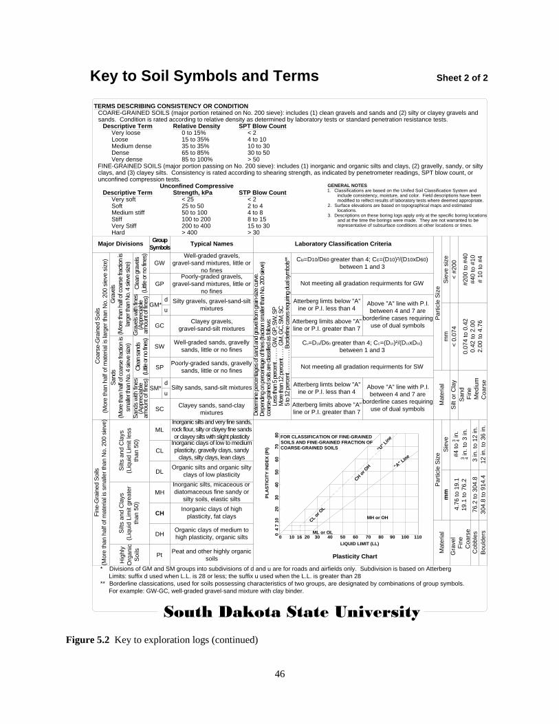
46

TERMS DESCRIBING CONSISTENCY OR CONDITIONCOARE-GRAINED SOILS (major portion retained on No. 200 sieve): includes (1) clean gravels and sands and (2) silty or clayey gravels andsands. Condition is rated according to relative density as determined by laboratory tests or standard penetration resistance tests.

Descriptive Term Relative Density SPT Blow CountVery loose 0 to 15% < 2Loose 15 to 35% 4 to 10Medium dense 35 to 35% 10 to 30Dense 65 to 85% 30 to 50Very dense 85 to 100% > 50

FINE-GRAINED SOILS (major portion passing on No. 200 sieve): includes (1) inorganic and organic silts and clays, (2) gravelly, sandy, or siltyclays, and (3) clayey silts. Consistency is rated according to shearing strength, as indicated by penetrometer readings, SPT blow count, orunconfined compression tests.

Unconfined CompressiveDescriptive Term Strength, kPa STP Blow Count

Very soft < 25 < 2Soft 25 to 50 2 to 4Medium stiff 50 to 100 4 to 8Stiff 100 to 200 8 to 15Very Stiff 200 to 400 15 to 30Hard > 400 > 30

GENERAL NOTES1. Classifications are based on the Unifed Soil Classification System and

include consistency, moisture, and color. Field descriptions have beenmodified to relfect results of laboratory tests where deemed appropriate.

2. Surface elevations are based on topographical maps and estimatedlocations.

3. Descriptions on these boring logs apply only at the specific boring locationsand at the time the borings were made. They are not warranted to berepresentative of subsurface conditions at other locations or times.

* Divisions of GM and SM groups into subdivisions of d and u are for roads and airfields only. Subdivision is based on Atterberg

Limits: suffix d used when L.L. is 28 or less; the suffix u used when the L.L. is greater than 28

** Borderline classications, used for soils possessing characteristics of two groups, are designated by combinations of group symbols.

For example: GW-GC, well-graded gravel-sand mixture with clay binder.

Major DivisionsGroup

SymbolsTypical Names Laboratory Classification Criteria

Part

icle

Siz

e

Sie

ve s

ize

mm

< 0

.074

< #

200

0.0

74 to 0

.42

0.4

2 to 2

.00

2.0

0 to 4

.76

#200 to #

40

#40 to #

10

# 1

0 to #

4

Sand

Fin

e

Me

diu

m

Coars

e

Silt

or

Cla

y

Ma

terial

Part

icle

Siz

e

mm

Sie

ve

4.7

6 to 1

9.1

19.1

to 7

6.2

#4 to 3 4

in.

3 4 in. to

3 in.

76.2

to 3

04.8

304.8

to 9

14.4

3 in. to

12 in.

12 in. to

36 in.

Ma

terial

Gra

vel

Fin

e

Coars

e

Cobble

s

Bould

ers

Det

erm

ine p

erce

ntag

es o

f sand

and

gra

vel fro

m g

rain

-size

curv

e.D

epen

ding

on

perc

enta

ge o

f fin

es

(fract

ion

smal

ler t

han

No.

200

sie

ve)

coars

e-gr

aine

d so

ils a

re c

lass

ified a

s fo

llow

s:Les

s th

an 5

per

cent

. . .

. . .

GW

, GP

, SW

, SP

Mor

e th

an 1

2 pe

rcen

t . .

. . .

GM

, GC

, SM

, SC

5 to

12 p

erce

nt .

. . .

. . .

. . .

Bor

derline

case

s re

quiring

dual

sym

bols**

Fin

e-G

rain

ed S

oils

(More

than h

alf

of m

ate

rial i

s s

malle

r th

an N

o. 200 s

ieve)

Coars

e-G

rain

ed S

oils

(More

than h

alf

of m

ate

rial i

s la

rger

than N

o. 200 s

ieve s

ize)

Hig

hly

Org

anic

Soils

Silt

s a

nd C

lays

(Liq

uid

Lim

it g

reate

r

than 5

0)

Silt

s a

nd C

lays

(Liq

uid

Lim

it less

than 5

0)

Sands

(More

than h

alf

of c

oars

e fr

act

ion is

smalle

r th

an N

o. 4

sie

ve s

ize)

Gra

vels

(More

than h

alf

of c

oars

e fr

act

ion is

larg

er th

an N

o. 4

sie

ve s

ize)

Sands

with

fines

(Appre

ciable

am

ount of fin

es)

Cle

an s

ands

(Little

or n

o fine

s)

Gra

vels

with

fines

(Appre

ciable

am

ount o

f fin

es)

Cle

an g

rave

ls

(Litt

le o

r no fi

nes)

GW

GP

GC

SW

SP

SC

ML

CL

DL

MH

CH

DH

Pt

SM*d

u

GM*d

u

Well-graded gravels,

gravel-sand mixtures, little or

no finesPoorly-graded gravels,

gravel-sand mixtures, little or

no fines

Silty gravels, gravel-sand-silt

mixtures

Clayey gravels,

gravel-sand-silt mixtures

Well-graded sands, gravelly

sands, little or no fines

Poorly-graded sands, gravelly

sands, little or no fines

Silty sands, sand-silt mixtures

Clayey sands, sand-clay

mixtures

Inorganic silts and very fine sands,

rock flour, silty or clayey fine sands

or clayey silts with slight plasticityInorganic clays of low to medium

plasticity, gravelly clays, sandy

clays, silty clays, lean clays

Organic silts and organic silty

clays of low plasticity

Inorganic silts, micaceous or

diatomaceous fine sandy or

silty soils, elastic silts

Inorganic clays of high

plasticity, fat clays

Organic clays of medium to

high plasticity, organic silts

Peat and other highly organic

soils

Cu=D10/D60 greater than 4; Cc=(D10)²/(D10xD60)

between 1 and 3

Not meeting all gradation requirments for GW

Atterberg limts below "A"

ine or P.I. less than 4

Atterberg limits above "A"

line or P.I. greater than 7

Above "A" line with P.I.

between 4 and 7 are

borderline cases requiring

use of dual symbols

Not meeting all gradation requirments for SW

Atterberg limts below "A"

ine or P.I. less than 4

Atterberg limits above "A"

line or P.I. greater than 7

Above "A" line with P.I.

between 4 and 7 are

borderline cases requiring

use of dual symbols

Cu=D10/D60 greater than 4; CC=(D10)²/(D10xD60)

between 1 and 3

0 10 16 20 30 40 50 60 70 80 90 100 110

"U" Lin

e

"A"

Line

MH or OH

ML or OL

CL o

r OL

CH o

r O

H

FOR CLASSIFICATION OF FINE-GRAINED

SOILS AND FINE-GRAINED FRACTION OF

COARSE-GRAINED SOILS

LIQUID LIMIT (LL)

PL

AS

TIC

ITY

IN

DE

X (

PI)

Plasticity Chart


Key to Soil Symbols and Terms Sheet 2 of 2

0

4 7

10

20

3

0

4

0

5

0

6

0

7

0

8

0

Figure 5.2 Key to exploration logs (continued)

47

Site & Exploration Plan - Big Sioux River

B-2

B-1N

Scale in Feet

0 40 80

Image taken from South Dakota

Department of Highways, 436'-0"

Cont. Comp. Gird. Viaduct over Big

Sioux River, Drawing 1 of 11 (June

1962).

Figure 5.3 Site and exploration plan for the Big Sioux River study site

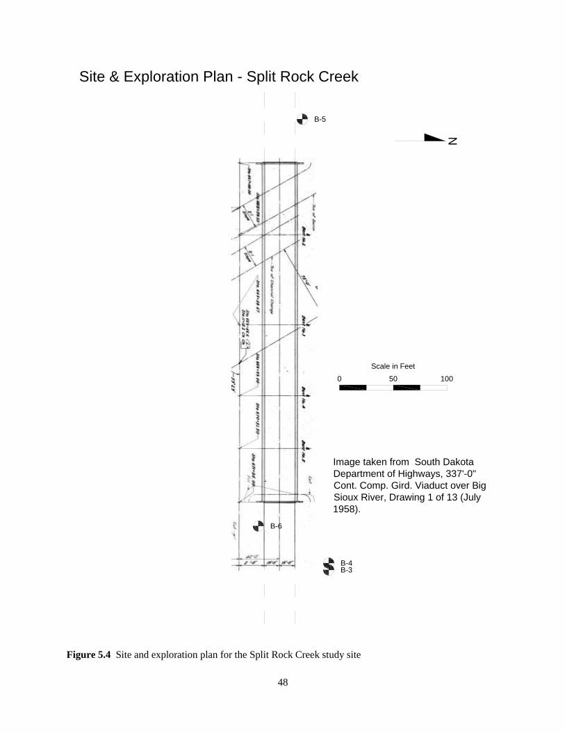
48

B-6

Site & Exploration Plan - Split Rock Creek

B-3

B-5N

B-4

Image taken from South Dakota

Department of Highways, 337'-0"

Cont. Comp. Gird. Viaduct over Big

Sioux River, Drawing 1 of 13 (July

1958).

Scale in Feet

0 50 100

Figure 5.4 Site and exploration plan for the Split Rock Creek study site

49

Site & Exploration Plan - White River

B-8

N

B-4B-9

B-10

Image taken from South Dakota State

Highway Commission, 337'-0" Cont.

Comp. Gird. Viaduct over Big Sioux

River, Drawing 1 of 11 (July 1948).

Scale in Feet

0 50 100

Figure 5.5 Site and exploration plan for the White River study site

B-7

B-9

50

Log of Boring B-1

Sheet 1 of 2

Project Location: Flandreau, SDProject Number: SD2006 - 08

Project: Evaluation of SRICOS Method


Ele

va

tio

n

De

pth

Typ

e

Nu

mb

er

Sa

mp

ling

Re

sis

tan

ce

Re

co

ve

ry,

%

Wa

ter

Co

nte

nt,

%

SAMPLES

feet


Date(s)Drilled

DrillingMethod

Drill RigType

GroundwaterLevel(s)

BoreholeBackfill

Logged By

Drill BitSize/Type

DrillingContractor

SamplingMethod(s)

Location

Checked By

Total Depthof Borehole

SurfaceElevation

HammerData

0

6-12-07

HSA

Mobil B57

18 ft.

Drill cuttings

A. Jones / R. Larsen

OD= 6 in. ID= 3.25 in.

GeoTek Engr. & Testing

Shelby Tube / SPT

Flandreau, SD, Highway 13 bridge over the Big Sioux River, 107 feet north, 7

feet east from the northwest corner of the north abutment.

55.5 ft.

1543 ft. *

Standard Trip Hammer

5

10

15

20

25

30

S-1 6 66

S-2A

S-2B9 66

S-3 10 44

S-4 15 55

S-5A

S-5B15 66

S-6 28 66

S-8 2 100

P-7 100

S-9 11 77

S-10

Four and one-half inches of asphalt concrete over fourteen

inches of base coarse over medium stiff, brown to gray,

moist, gravelly, sandy silt (fill).

Stiff, brown, moist, sandy silt/clay (fill).

Stiff, mottled brown/gray, moist, slightly sandy silt

(fill).

Very stiff, mottled white/brown/black, moist to dry, gravelly

sandy silt (fill).

Soft, gray, wet, very silty fine sand.

PP = 0.5 tsf

Medium dense, gray, wet, coarse sand. 24 in. of heave.

A. Jones

Start at 07:15.

12

15

18

17

17

6

30

31

17

19

17

Figure 5.6 Log of boring B-1

51

Log of Boring B-1

Sheet 2 of 2




Ele

va

tio

n

De

pth

Typ

e

Nu

mbe

r

Sa

mplin

gR

esis

tan

ce

Re

co

very

, %

Wate

rC

on

ten

t, %

SAMPLES

feet


30

35

40

45

50

55

60

65

S-10 10 55

S-11 6 33

S-12 12 55

S-13 60 50

S-14 22 83

P-15 100

P-16 77

Medium dense, gray, wet, gravelly sand. 18 in. of heave.

Medium dense, gray, wet, medium sand.

Very dense, grayto brown, wet, coarse to medium sand.

Very stiff, gray, moist, sandy silt/clay (possible glacial till).

Brown to gray, moist, slightly sandy clay.PP = 3.5 tsf

End at 09:45.

18 in. of heave.

9

9

9

9

9

* Elevation referenced to lower steel at north abutment.

Elevation taken from Scour Assessments And

Sediment-Transport Simulation For Selected Bridge Sites

In South Dakota prepared by Colin A. Niehus (1996).

Figure 5.7 Log of boring B-1 (continued)

52

Log of Boring B-2

Sheet 1 of 2




Ele

va

tio

n

De

pth

Typ

e

Nu

mbe

r

Sa

mp

ling

Re

sis

tan

ce

Re

co

ve

ry,

%

Wa

ter

Co

nte

nt,

%

SAMPLES

feet


Date(s)Drilled

DrillingMethod

Drill RigType

GroundwaterLevel(s)

BoreholeBackfill

Logged By

Drill BitSize/Type

DrillingContractor

SamplingMethod(s)

Location

Checked By


SurfaceElevation

HammerData

0

6-12-07

HSA

Mobil B57

33 ft.

Drill cuttings


OD= 6 in. ID= 3.25 in.


Shelby Tube / SPT

51 ft.

1547 ft.*


5

10

15

20

25

30

S-1 6 61

S-2 7 38

S-3 8 50

S-4 8 66

S-5 9 55

S-6 18 55

S-7 8 83

P-8 88

S-9A23 88

P-12

Six inches of asphalt concrete over eighteen inches of

base coarse over loose, dark gray to dark brown, moist,

gravelly very sitly sand (fill).

Loose, brown, moist to wet, very silty sand with some

gravel (fill).

Stiff, gray to tan, moist, fine sandy silt (fill).

Medium dense, brown, moist to wet, slightly gravelly, very

silty, fine to coarse sand (fill).

Medium stiff, gray, moist, slightly gravelly slightly sandy silt.

PP > 4.5 tsf

Medium stiff, brown to gray, moist, fine sandy silt (fill).

S-9B

Very stiff, brown, moist, silty clay

Very stiff, mottled gray, moist, very sandy silt

P-10 100 PP = 0.75 tsfMedium dense, gray, moist to wet, silty sand with some

gravel.S-11A27 94S-11B

Medium dense, gray moist, slightly gravelly sand

Flandreau, SD, Highway 13 bridge over the Big Sioux River, 100 feet south, 6

feet east from the southwest corner of the south abutment.

A. Jones

Start at 10:00.

Black, moist, organic silt with abundant organic fibers.

6

16

16

15

15

9

11

9

10

17

12


53

Log of Boring B-2

Sheet 2 of 2

Project Location: Flandreua, SDProject Number: SD2006 - 08



Ele

va

tio

n

De

pth

Typ

e

Nu

mbe

r

Sa

mplin

gR

esis

tan

ce

Re

co

very

, %

Wate

rC

on

ten

t, %

SAMPLES

feet


30

35

40

45

50

55

60

65

100

S-13 2 100

S-19 13 100

P-20 100

Soft, black, wet, very silty fine sand to very fine sandy silt.

Medium stiff, mottled gray/tan, moist clay/silt with fine

gravel. PP > 4.5 tsf

End at 12:20.

P-12 Soft, black, moist to wet, organic silt with abundant organic

fibers.PP = 2.75 tsf

100P-14Loose, dark brown to black, wet, silty fine sand.

PP = 1.25 tsf

S-15A7 66

Loose, tan/gray, wet, sandy gravel.

S-15B Medium stiff, brown & tan, moist to wet, very sandy silt

100P-16 PP > 4.5 tsf

S-17 18 77

100P-18 PP = 2.5 tsf

48

28

28

12

20

20

23

* Elevation referenced to lower steel at south abutment.





54

Log of Boring B-3

Sheet 1 of 1

Project Location: Brandon, SDProject Number: SD2006-08



Ele

va

tio

n

De

pth

Type

Num

be

r

Sam

plin

gR

esis

tance

Reco

ve

ry, %

Wa

ter

Con

ten

t, %

SAMPLES

feet


Date(s)Drilled

DrillingMethod

Drill RigType

GroundwaterLevel(s)

BoreholeBackfill

Logged By

Drill BitSize/Type

DrillingContractor

SamplingMethod(s)

Location

Checked By


SurfaceElevation

HammerData

0

07-17-07

HSA

B57

None

Drill cuttings


OD= 6 in. ID= 3.25 in.


Shelby Tube/ SPT

25.6 ft.

1338 ft.*


5

10

15

20

25

30

S-1 11 83

S-2 11 83

S-3 8 78

S-4 7 100

S-5 11 83

S-6 13 94

S-8 13 100

P-7 100

S-9 56/7" 100

Start at 07:30.

Stiff, mottled, brown, black, & gray, moist, slightly gravelly

fine sandy silt.

Mottled, light tan & brown, moist clay.

PP=2.0 tsf

Medium dense to stiff, light brown to mottled tan, moist,

gravelly silty fine sand to gravelly fine sandy silt (fill).

Perched water.

Medium dense, mottled, tan, moist, very silty fine sand.

White, moderately weathered silt stone.

19

21

21

23

19

18

33

A. Jones

Brandon, SD, I-90 bridge over Split-Rock Creek, 67 feet east, 33 feet north,

from the northeast corner of the east abutment.

Stop at 08:30.* Elevation referenced to lower steel at east abutment.

Elevation taken from Analysis of Scour Potential for

Bridge Structures Nos. 50-284-165 and 50-284-166 Split

Rock Creek Near Brandon, SD Interstates 90 East and

West Appendix 6 prepared by Colin A. Niehus (Jan 1993).


55

Log of Boring B-4

Sheet 1 of 1




Ele

va

tio

n

De

pth

Type

Num

be

r

Sam

plin

gR

esis

tance

Reco

ve

ry, %

Wa

ter

Con

ten

t, %

SAMPLES

feet


Date(s)Drilled

DrillingMethod

Drill RigType

GroundwaterLevel(s)

BoreholeBackfill

Logged By

Drill BitSize/Type

DrillingContractor

SamplingMethod(s)

Location

Checked By


SurfaceElevation

HammerData

0

07-17-07

HSA

B57

None

Drill cuttings


OD= 6 in. ID= 3.25 in.


Shelby Tube

22.0 ft.

1338 ft.*


5

10

15

20

25

30

P-2 67

Drilled without sampling to 12.0-foot-depth.

Mottled, brown, black, & gray, moist, slightly gravelly fine

sandy silt.

Mottled, light tan & brown, moist, clay.

PP = 1.25 tsf

PP = 3.5 tsfP-1 83

A. Jones

Brandon, SD, I-90 bridge over Split-Rock Creek, 62 feet east, 33 feet north,

from the northeast corner of the east abutment.

Start at 08:40.

End at 09:00.

16

* Elevation referenced to lower steel at east abutment.




West Appendix 6 prepared by Colin A. Niehus (Jan

1993).


56

Log of Boring B-5

Sheet 1 of 2




Ele

va

tio

n

De

pth

Typ

e

Nu

mb

er

Sa

mp

ling

Re

sis

tan

ce

Re

co

ve

ry,

%

Wa

ter

Co

nte

nt,

%

SAMPLES

feet


Date(s)Drilled

DrillingMethod

Drill RigType

GroundwaterLevel(s)

BoreholeBackfill

Logged By

Drill BitSize/Type

DrillingContractor

SamplingMethod(s)

Location

Checked By


SurfaceElevation

HammerData

0

07-17-07

HSA

B57

26.0 ft

Drill cuttings


OD= 6 in. ID= 3.25 in.


Shelby Tube / SPT

34.7 ft.

1334 ft.*


5

10

15

20

25

30

P-10 100

Start at 09:20.

PP = 2.75 tsfP-5 71

Loose to stiff, brown & gray, moist, very silty sand to

slightly gravelly fine sandy silt (fill).

S-1 617

S-2 897

S-3 899

S-4 8913

S-6A10013

S-6BStiff, mottled, black & gray, moist, fine sandy silt. PP = 3.0 tsf

P-7 100

Medium dense, black, moist to dry, very silty sand.S-8 10019

P-9 100 Loose, interbedded black & white, moist, slightly silty

gravelly sand to slightly gravelly medium sand.PP=1.0 tsf

S-11 1005

P-12 33 Loose to medium dense, brown & black, wet, gravelly

medium sand to slightly sandy gravel.

S-13 723

S-14 7212

S-15 174

13

15

12

30

21

20

19

22

Brandon, SD, I-90 bridge over Split-Rock Creek, 43 feet west, 6 feet north,

from the northwest corner of the west abutment.

A. Jones

19


57

Log of Boring B-5

Sheet 2 of 2




Ele

va

tio

n

De

pth

Typ

e

Nu

mb

er

Sa

mp

ling

Re

sis

tan

ce

Re

co

ve

ry,

%

Wa

ter

Co

nte

nt,

%

SAMPLES

feet


30

35

40

45

50

55

60

S-15 Loose, gray, wet, slightly gravelly coarse sand.

S-16 444

White, moderately weatherd silt stone.S-17 1150/2"

Stop at 10:50.

65

* Elevation referenced to lower steel at east abutment.




West Appendix 6 prepared by Colin A. Niehus (Jan

1993).


58

Log of Boring B-6

Sheet 1 of 1




Ele

vation

Depth

Type

Num

ber

Sam

plin

gR

esis

tance

Recovery

, %

Wate

rC

onte

nt, %

SAMPLES

feet


Date(s)Drilled

DrillingMethod

Drill RigType

GroundwaterLevel(s)

BoreholeBackfill

Logged By

Drill BitSize/Type

DrillingContractor

SamplingMethod(s)

Location

Checked By


SurfaceElevation

HammerData

0

07-17-07

HSA

B57

21.0 ft

Drill cuttings


OD= 6 in. ID= 3.25 in.


Shelby Tube / SPT

27.8 ft.

1343 ft.*


5

10

15

20

25

30

Start at 12:10.Medium dense to loose, brown, moist, very silty sand to

slightly gravelly very silty sand (fill).

S-1 7811

S-2 568

S-3 6710

Medium stiff to stiff, light brown & tan, moist, very sandy

silt.S-4 834

P-6 83Mottled, light brown/gray, moist silty clay.

S-5 6711

S-7 836

P-8 88 Loose, light brown, moist, very silty fine sand.

S-9 1005

P-10 100 Medium stiff, mottled, gray & light brown, moist, silty clay.

S-11 837

P-12 83

S-13 10053/10" White, moderately weathered silt stone.

11

15

19

24

20

24

24

23

Brandon, SD, I-90 bridge over Split-Rock Creek, 19 feet east, 6 feet south,

from the southeast corner of the east abutment.

A. Jones

Stop at 13:10.

26

25

* Elevation referenced to lower steel at east abutment. Elevation taken

from Analysis of Scour Potential for Bridge Structures Nos. 50-284-165

and 50-284-166 Split Rock Creek Near Brandon, SD Interstates 90

East and West Appendix 6 prepared by Colin A. Niehus (Jan 1993).


59

Log of Boring B-7

Sheet 1 of 2

Project Location: Presho, SDProject Number: SD2006-08



Ele

va

tio

n

De

pth

Typ

e

Nu

mb

er

Sa

mp

ling

Re

sis

tan

ce

Re

co

ve

ry,

%

Wa

ter

Co

nte

nt,

%

SAMPLES

feet


Date(s)Drilled

DrillingMethod

Drill RigType

GroundwaterLevel(s)

BoreholeBackfill

Logged By

Drill BitSize/Type

DrillingContractor

SamplingMethod(s)

Location

Checked By


SurfaceElevation

HammerData

0

10-11-07

HSA

B57

26.0 ft

Drill cuttings


OD= 6 in. ID= 3.25 in.


Shelby Tube / SPT

35.5 ft.

1596 ft. *


5

10

15

20

25

30

Start at 08:00.Medium stiff, brown, moist, slightly sandy to slightly

gravelly silt (fill).

S-1 176

S-2 666

S-3 613

Stiff, gray to brown, moist, silt.S-4 1006

P-6 67

S-5 1008

S-7 10014

S-9 1009

P-10 100

31

31

38

38

33

33

29

Presho, SD, White River, 19 feet north, 6 feet east, from the northwest corner

of the north abutment.

P-8 92

S-11 1009 41

P-12 75 Medium dense, brown, moist to wet, silty sandy gravel.

PP = 3.5 tsf

PP = 3.25 tsf

PP = 2.75 tsf

A. Jones


60

Log of Boring B-7

Sheet 2 of 2

Project Location: Presho SDProject Number: SD2006-08



Ele

va

tio

n

De

pth

Typ

e

Nu

mb

er

Sa

mp

ling

Re

sis

tan

ce

Re

co

ve

ry,

%

Wa

ter

Co

nte

nt,

%

SAMPLES

feet


30

35

40

45

50

55

60

4418

Stop at 09:20.

65

Gray, slightly weathered, shale.

S-13AS-13B

16

10050S-14






61

Log of Boring B-8

Sheet 1 of 1




Ele

vation

Depth

Type

Num

ber

Sam

plin

gR

esis

tance

Recovery

, %

Wate

rC

onte

nt, %

SAMPLES

feet


Date(s)Drilled

DrillingMethod

Drill RigType

GroundwaterLevel(s)

BoreholeBackfill

Logged By

Drill BitSize/Type

DrillingContractor

SamplingMethod(s)

Location

Checked By


SurfaceElevation

HammerData

0

10-11-07

HSA

B57

None

Drill cuttings


OD= 6 in. ID= 3.25 in.


Shelby Tube / SPT

28.5 ft.

1586 ft. *


5

10

15

20

25

30

Start at 09:50.Loose to medium dense, brown, moist, slightly silty sand

(fill).

S-1 1006

S-2 10015

S-3A 1005Loose, black to tan, moist, fine silty sand.

10010

S-5 675

S-7 786

S-9 783

7

10

10

6

22

28

Presho, SD, White River, 20 feet south, 8 feet east, from the southwest

corner of the south abutment.

S-11 10049

S-3B

S-4A

S-4B

S-6 898

S-8 783

S-10 677

Stop at 10:50.

10

24

3

15

22

15

Loose, tan, moist, fine to coarse sand.

Loose, brown, moist, slightly sandy gravel.

Loose, brown, moist, silty medium to coarse sand.


A. Jones






62

Log of Boring B-9

Sheet 1 of 1




Ele

va

tio

n

De

pth

Type

Num

be

r

Sam

plin

gR

esis

tance

Reco

ve

ry, %

Wa

ter

Con

ten

t, %

SAMPLES

feet


Date(s)Drilled

DrillingMethod

Drill RigType

GroundwaterLevel(s)

BoreholeBackfill

Logged By

Drill BitSize/Type

DrillingContractor

SamplingMethod(s)

Location

Checked By


SurfaceElevation

HammerData

0

10-11-07

HSA

B57

None

Drill cuttings


OD= 6 in. ID= 3.25 in.


Shelby Tube

31.0 ft.

1596 ft. *


5

20

25

30

35

40

Start at 11:10.No sampling to 24 ft-depth.

Presho, SD, White River, 20 feet north, 9 feet east, from the northwest corner

of the north abutment.

100

Stop at 11:40.

P-1

79P-2

A. Jones






63

Log of Boring B-10

Sheet 1 of 1




Ele

va

tio

n

De

pth

Type

Num

be

r

Sam

plin

gR

esis

tance

Reco

ve

ry, %

Wa

ter

Con

ten

t, %

SAMPLES

feet


Date(s)Drilled

DrillingMethod

Drill RigType

GroundwaterLevel(s)

BoreholeBackfill

Logged By

Drill BitSize/Type

DrillingContractor

SamplingMethod(s)

Location

Checked By


SurfaceElevation

HammerData

0

10-11-07

HSA

B57

10 ft

Drill cuttings


OD= 6 in. ID= 3.25 in.


Shelby Tube / SPT

22.0 ft.

1582 ft. *


5

10

15

20

25

30

Start at 12:15.Loose to very loose, tan, dry to wet, very silty fine sand.

Presho, SD, White River, 120 feet north, 36 feet east, from the northeast

corner of the south abutment.

72

Stop at 12:55.

S-1

P-7

4 5

61S-2 3 8

78S-3 2 11

83S-4 7 24

61S-6 1/12" 23

39S-8 5 28

S-9 30

P-5 100

96 Loose, gray, wet, slightly silty very sandy gravel.


A. Jones






64

1560

650

600

550

500

450

400

350

300

250

200

150

100

50

1550

1540

1530

1520

1510

1500

1490

6 9 10

15

15

28 P 2 11

10 6 12

1480

60

22 P P

Horizonta

l S

cale

in F

eet

Vert

ica

l S

cale

in F

eet

Vert

ica

l E

xag

gera

tion x

5

0050

100

10

20

1560

1550

1540

1530

1520

1510

1500

1490

1480

6 7 8 8 9 18 8 P 23 P 27 P 2 P 7 P 18 P 13 P

B-1

B-2

6 P

B-1

Legend

Borin

g N

um

ber

Sta

ndard

Pene

tratio

n R

esis

tance

in B

low

s p

er

Foot

She

lby T

ube

Sam

ple

Scou

r B

ed 7

-7-9

3

Ori

gin

al B

ed 3

-30-9

3

0

Elevation in Feet

Dis

tance f

rom

B-2

in F

eet

Elevation in Feet

Fill

Gra

y, very

silt

y fin

e s

and

Gra

y, coa

rse g

ravelly

sand

Gra

y, m

ediu

m s

and

Gra

y/b

row

n, coars

e/m

ed

ium

sand

Gra

y, san

dy s

ilt/c

lay

Bro

wn/tan/g

ray, very

sandy

silt

/cla

y

Dark

bro

wn/b

lack, silt

y fin

e s

and

Bla

ck s

ilt/o

rga

nic

silt

w/ fine

org

anic

fib

ers

Gra

y, slig

htly g

ravelly

sand

Bro

wn,

silt

y c

lay

Gra

y, slig

htly g

ravelly

sandy s

ilt

Fill

Gro

und W

ate

r at

Tim

e o

f D

rilli

ng

Genera

lized S

ubsurf

ace P

rofile

A-A

' - B

ig S

ioux R

iver

?

?

? ? ?

?

? ? ? ? ?

Infe

rred S

oil

Boundary

?

Bottom

of S

teel*

* B

otto

m o

f ste

el re

fere

nced to S

co

ur

Assessm

ents

And S

edim

en

t-T

ransp

ort

Sim

ula

tion

For

Sele

cte

d B

ridge S

ites I

n S

outh

Dakota

pre

pare

d b

y C

olin

A.

Nie

hus (

1996).

Roadw

ay D

eck

Figure 5.20 Generalized subsurface profile for the Big Sioux River study site

65

520

480

440

400

360

320

280

240

200

160

120

80

40

1350

1340

1330

1320

1310

1300

1290

Horizonta

l S

cale

in F

eet

Vert

ica

l S

cale

in F

eet

Vert

ica

l E

xag

gera

tion x

4

0040

80

10

20

1350

1340

1330

1320

1310

1300

1290

0

Elevation in Feet

Dis

tance f

rom

B-3

in F

eet

Elevation in Feet

11

11 8 7 11

13 P 13

56

/ 7

in

.

7 7 9 13 P

B-3

B-5

13 P 19 P P 5 P 3 12 4 4

50

/ 2

in

.

Fill

Bro

wn,

slig

htly g

rave

lly f

ine s

andy s

ilt

Lig

ht bro

wn, cla

y

Tan, ve

ry s

ilty f

ine s

and

White

, m

odera

tely

weath

ere

d s

ilt s

tone

White

, m

odera

tely

weath

ere

d s

ilt s

tone

Bla

ck, gra

velly

mediu

m

sand

Bla

ck,

very

silt

y s

and

Fill

Ge

ne

raliz

ed S

ubsu

rface P

rofile

A-A

' - S

plit

Rock C

reek

6 P

B-1

Legend

Borin

g N

um

ber

Sta

ndard

Pene

tratio

n R

esis

tance

in B

low

s p

er

Foot

She

lby T

ube

Sam

ple

Scou

r B

ed 5

-8-9

3

Ori

gin

al B

ed 3

-29-9

3

Gro

und W

ate

r at

Tim

e o

f D

rilli

ng

1280

1280

??

??

???

?

?

Infe

rred S

oil

Boundary

?

Bottom

of S

teel*

* B

otto

m o

f ste

el re

fere

nced to A

na

lysis

of S

cour

Pote

ntial F

or

Bridge S

tructu

re N

os.

50-2

84-1

65 a

nd 5

0-2

84-1

66 S

plit

Rock C

reek N

ear

Bra

ndon,

SD

Inte

rsta

tes 9

0 E

ast

and

West

Ap

pendix

6 p

repare

d b

y C

olin

A.

Nie

hus (

Jan 1

99

3).

Roadw

ay D

eck

Figure 5.21 Generalized subsurface profile for the Split Rock Creek study site

66

48

04

40

40

03

60

32

02

80

24

02

00

16

01

20

80

40

Hori

zon

tal S

cale

in F

eet

Vert

ical S

ca

le in F

eet

Vert

ical E

xa

gg

era

tion x

4004

08

0

10

20

16

10

16

00

15

90

15

80

15

70

15

60

15

50

0

Dis

tan

ce

fro

m B

-7 in

Fe

et

Elevation in Feet

6 6 3 6 8 14P 9

6 15 5 10

B-7

B-8

5 8 6 3 3 7 49

Genera

lized S

ub

surf

ace P

rofile

A-A

' - W

hite R

iver

6 P

B-1

Legend

Bo

rin

g N

um

be

r

Sta

nd

ard

Pe

ne

tra

tio

n R

esis

tan

ce

in

Blo

ws p

er

Fo

ot

Sh

elb

y T

ub

e S

am

ple

Sco

ur

Be

d 0

5-0

8-9

3

Ori

gin

al B

ed

08

-22

-91

Gro

un

d W

ate

r a

t T

ime

of D

rilli

ng

15

40

Infe

rre

d S

oil

Bo

un

da

ry?

9P P P 18

50

Bo

ttom

of S

teel*

16

10

16

00

15

90

15

80

15

70

15

60

15

50

15

40

?

??

??

?

?

Fill

Bro

wn to g

ray, silt

?B

row

n, silt

y s

andy g

ravell

Gra

y s

hale

?

Bro

wn, slig

htly s

andy g

ravel

Gra

y s

hale

Bro

wn, silt

y m

ediu

m c

oars

e s

and

Tan, fine to

coars

e s

and

Bla

ck, fine s

ilty s

and

?

Fill

??

* B

ott

om

of

ste

el re

fere

nce

d t

o S

co

ur

Asse

ssm

en

ts A

nd

Se

dim

en

t-T

ran

sp

ort

Sim

ula

tio

n

Fo

r S

ele

cte

d B

rid

ge

Site

s I

n S

ou

th D

akto

a p

rep

are

d b

y C

olin

A. N

ieh

us (

19

96).

** B

-9 o

ve

rla

ys B

-7.

It

is o

ffse

t to

sh

ow

sa

mple

s

PP

B-9

**

4 3 2 7

B-1

0 *

**

1/1

2"

5 30P P

***

B-1

0 is 3

6 f

ee

t e

ast

of

the

brid

ge

de

ck

Roa

dw

ay D

eck

Figure 5.22 Generalized subsurface profile for the White River study site

67

Plasticity Chart

0

10

20

30

40

50

60

70

0 10 20 30 40 50 60 70 80 90 100

Liquid Limit (LL)

Pla

sti

cit

y I

nd

ex (

PI)

B-2 P-12

B-2 P-14

B-6 P-6

B-4 P-2

B-4 P-2

B-7 P-10

B-9 P-1

B-7 P-12

Figure 5.23 Laboratory testing results for atterberg limit testing

68

Hydrometer Analysis

0

10

20

30

40

50

60

70

80

90

100

0.0010.0100.1001.000

Diameter of Soil Particles (mm)

Pe

rce

nt

of

So

il S

us

pe

nd

ed

B-10 P-5

B-10 P-7

B-5 P-10

B-1 P-7

B-2 P-14

B-4 P-2

B-6 P-8

B-6 P-6

B-9 P-1

B-7 P-12

B-7 P-10

B-2 P-12

Figure 5.24 Laboratory testing results for hydrometer analysis testing

69

No. 200 Wash

0

10

20

30

40

50

60

70

80

90

100

0.0010.010.11

Diameter of Soil Particles (mm)

Perc

en

t o

f S

oil

Su

sp

en

ded

B-1 P-7

B-2 P-12

B-2 P-14

B-4 P-2

B-5 P-10

B-6 P-6

B-6 P-8

B-7 P-10 B-7 P-12

B-9 P-1

B-10 P-5

B-10 P-7

Figure 5.25 Laboratory testing results for No. 200 wash analysis

71

6. RESULTS OF EFA TESTS 6.1 Big Sioux River Bridge

Tables 6.1 to 6.3 summarize the EFA test results from the Big Sioux River Bridge. The test results are

plotted in Figures 6.1 to 6.3. In these tables, and others to follow, V is the cross-sectional average

velocity, Re is the Reynolds number, τ is the applied bed shear stress, ε is the bed roughness height, ∆z is

the amount of soil erosion, and ∆t is the time to erode ∆z. The formulae for calculating τ are given in

Section 6.4.

Table 6.1 EFA test results for Big Sioux River Bridge; boring B-1 P-7, depth 19.5 to 21.5 ft, very silty

fine sand, test 1 (first table) and test 2 (second table).

V (m/s) Re τ (N/m

2)

(ε = 0 mm)

τ (N/m2)

(ε = 1 mm)

τ (N/m2)

(ε = 2 mm)

τ (N/m2)

(ε = 3 mm)

Δz

(mm)

Δt

(s)

Δz/Δt

(mm/hr)

0.173 11717 0.11 0.18 0.22 0.26 0 137 0.0

0.335 22689 0.36 0.64 0.81 0.96 0 560 0.0

0.473 32036 0.66 1.25 1.61 1.91 0 613 0.0

0.628 42534 1.08 2.19 2.83 3.35 0 600 0.0

0.773 52355 1.56 3.30 4.27 5.07 0 600 0.0

1.028 69625 2.57 5.81 7.54 8.96 0 600 0.0

1.177 79717 3.25 7.60 9.87 11.73 0 600 0.0

1.352 91570 4.14 10.01 13.01 15.47 0 569 0.0

1.451 98275 4.69 11.52 14.98 17.82 0 600 0.0

1.682 113920 6.07 15.46 20.11 23.93 0 569 0.0

1.894 128279 7.47 19.58 25.49 30.33 0 462 0.0

2.126 143992 9.15 24.65 32.10 38.20 11 853 46.4

2.388 161737 11.21 31.07 40.49 48.18 11 375 105.6

2.611 176841 13.11 37.13 48.39 57.59 11 294 134.7

1.703 115343 6.21 15.84 20.62 24.53 0 1124 0.0

1.905 129024 7.55 19.81 25.79 30.68 0 1124 0.0

2.044 138438 8.54 22.79 29.68 35.31 11 1124 35.2

2.265 153406 10.22 27.96 36.43 43.35 11 500 79.2

2.565 173725 12.71 35.83 46.70 55.58 11 284 139.4

2.702 183004 13.92 39.75 51.81 61.67 10 254 141.7

72


organic silt with abundant organic fibers.

V (m/s) Re τ (N/m

2)

(ε = 0 mm)

τ (N/m2)

(ε = 1 mm)

τ (N/m2)

(ε = 2 mm)

τ (N/m2)

(ε = 3 mm)

Δz

(mm)

Δt

(s)

Δz/Δt

(mm/hr)

0.333 22554 0.36 0.63 0.80 0.95 0 601 0.0

0.637 43142 1.11 2.25 2.91 3.45 0 600 0.0

0.994 67323 2.42 2.43 7.05 8.37 0 1200 0.0

1.147 77685 3.11 7.22 9.37 11.14 0 1200 0.0

1.455 98546 4.71 11.58 15.06 17.91 0 1200 0.0

1.712 115952 6.26 16.01 20.84 24.79 0 1200 0.0

1.940 131394 7.79 20.54 26.74 31.82 0 1200 0.0

2.213 149884 9.81 26.70 34.78 41.39 0 1200 0.0

2.424 164175 11.51 32.01 41.71 49.64 11 1275 31.1

2.558 173251 12.65 35.64 46.44 55.28 11 1527 25.9


silty fine sand.

V (m/s) Re τ (N/m

2)

(ε = 0 mm)

τ (N/m2)

(ε = 1 mm)

τ (N/m2)

(ε = 2 mm)

τ (N/m2)

(ε = 3 mm)

Δz

(mm)

Δt

(s)

Δz/Δt

(mm/hr)

0.182 12327 0.12 0.19 0.24 0.29 0 606 0.0

0.214 14494 0.16 0.27 0.34 0.40 0 594 0.0

0.253 17135 0.22 0.37 0.47 0.55 0 600 0.0

0.293 19845 0.29 0.49 0.62 0.74 0 165 0.0

0.332 22486 0.35 0.62 0.80 0.94 0 600 0.0

0.399 27024 0.49 0.90 1.15 1.36 11 258 153.5

0.417 28243 0.53 0.98 1.25 1.48 4 721 20.0

0.418 28311 0.53 0.98 1.26 1.49 11 139 284.9

0.497 33661 0.72 1.38 1.78 2.10 10 137 262.8

0.499 33797 0.72 1.39 1.79 2.12 11 72 550.0

0.647 43821 1.14 2.32 3.00 3.56 11 114 347.4

0.659 44633 1.18 2.41 3.11 3.69 17 974 62.8

1.095 74163 2.86 6.58 8.55 10.16 1 754 4.8

73


depth 19.5 to 21.5 ft, very silty fine sand, tests 1 and 2


depth 29.5 to 31.5 ft , organic silt with abundant organic fibers.

74


depth 34.0 to 36.0 ft, silty fine sand. The bed shear stress is for ε = 1 mm.

Figure 6.1 shows the measured erosion rate versus shear stress curve for boring B-1 P-7 from the right

(north) abutment. The elevation of the sample (1,521.5 to 1,523.5 ft) was close to the initial elevation of

the channel bottom (1,520.72 ft; June 22, 1992) at the northern-most pier (bent 2) (see Figure 5.20). The

soil was classified as soft, gray, wet, very silty fine sand. The threshold velocity for erosion was about

1.9 m/s. The soil eroded particle by particle more or less uniformly. The relatively high rate of erosion is

consistent with the deep scour hole observed around bent 2. Two sets of tests (1 and 2) were conducted

on the same thin wall tube sample on two separate days (see Table 6.1). When plotted together, the

results collapse on the same curve, which gives confidence to the repeatability of the tests. In Figure 6.1,

the erosion rate curve is presented for four different values of bed roughness height (ε = 0, 1, 2, and 3

mm). As seen, both the critical shear stress and the slope of the erosion rate curve change considerably

with the roughness height assumed. Increasing the ε value will increase the friction factor and thus the

calculated bed shear stress. However, the increase in bed shear stress is greater at high velocities than at

low velocities. Because of this, the critical shear stress increases and the slope of the erosion rate versus

shear stress curve decreases as the roughness height increases. Figure 6.1 was used with the SRICOS

method to predict the local scour at bent 2. The different erosion rate curves were used to conduct a

sensitivity analysis on the effects of critical shear stress and slope of erosion rate versus shear stress curve

on the predicted scour depths.

Figure 6.2 shows the measured erosion rate versus shear stress curve for boring B-2 P-12 from the left

(south) abutment. The elevation of the sample (1,515.5 to 1,517.5 ft) was close to the initial elevation of

the channel bottom (1,523.22 ft; June 22, 1992) at the southern-most pier (bent 4) (see Figure 5.20). The

soil was classified as soft, black, moist to wet, organic silt with abundant organic fibers. The threshold

velocity for erosion was about 2.2 m/s. This soil eroded particle by particle and in chunks. The measured

erosion rate was much smaller compared with the very silty fine sand from boring B-1 P-7. This is

consistent with the much lesser scour observed around bent 4. Figure 6.2 was used to predict the local

scour at bent 4.

75


(south) abutment. The soil was classified as loose, dark blown to black, wet, silty fine sand. The

threshold velocity for erosion was less than 0.5 m/s. The measured erosion rates were very high, but the

location of the sample suggests that this soil layer would lie below the scour envelope of the southern-

most pier (bent 4). Therefore, Figure 6.3 was not used for scour prediction. The erosion rate versus shear

stress curve is shown for ε = 1 mm as an example.

6.2 Split Rock Creek Bridges

Tables 6.4 to 6.8 summarize the EFA test results from the Split Rock Creek bridges. The test results are

plotted in Figures 6.4 to 6.8.

Table 6.4 EFA test results for Split Rock Creek bridges; boring B-4 P-2, depth 20.0 to 22.0 ft, clay

V (m/s) Re τ (N/m

2)

(ε = 0 mm)

τ (N/m2)

(ε = 1 mm)

τ (N/m2)

(ε = 2 mm)

τ (N/m2)

(ε = 3 mm)

Δz

(mm)

Δt

(s)

Δz/Δt

(mm/hr)

0.198 13409 0.14 0.23 0.29 0.34 0 600 0.0

0.260 17627 0.23 0.39 0.49 0.58 0 600 0.0

0.496 33561 0.72 1.37 1.77 2.10 0 600 0.0

0.644 43630 1.13 2.30 2.97 3.53 0 600 0.0

0.750 50799 1.48 3.11 4.02 4.78 0 580 0.0

0.794 53806 1.63 3.48 4.51 5.35 0 1224 0.0

0.878 59475 1.95 4.25 5.50 6.54 0 1560 0.0

0.952 64452 2.24 4.99 6.47 7.68 0 1200 0.0

1.186 80335 3.29 7.72 10.02 11.91 0 1200 0.0

1.421 96273 4.52 11.05 14.37 17.09 0 1200 0.0

1.997 135254 8.20 21.76 28.33 33.71 0 1264 0.0

2.348 159017 10.88 30.04 39.14 46.58 1 949 3.8

76


slightly silty gravelly sand to slightly gravelly medium sand

V (m/s) Re τ (N/m

2)

(ε = 0 mm)

τ (N/m2)

(ε = 1 mm)

τ (N/m2)

(ε = 2 mm)

τ (N/m2)

(ε = 3 mm)

Δz

(mm)

Δt

(s)

Δz/Δt

(mm/hr)

0.132 8968 0.07 0.11 0.13 0.15 0.0 600 0.0

0.276 18693 0.26 0.44 0.55 0.65 0.0 600 0.0

0.496 33609 0.72 1.37 1.77 2.10 4.0 1527 9.4

0.653 44234 1.16 2.36 3.06 3.63 5.0 1909 9.4

0.888 60114 1.98 4.34 5.62 6.68 11.0 1031 38.4

1.219 82550 3.46 8.15 10.58 12.58 3.5 2136 5.9

1.437 97299 4.61 11.29 14.68 17.47 11.0 567 69.8

1.505 101911 5.00 12.38 16.11 19.16 31.0 140 797.1

1.708 115653 6.23 15.93 20.73 24.67 21.0 105 720.0

Table 6.6 EFA Test Results for Split Rock Creek bridges; boring B-5 P-12, depth 23.5 to 25.5 ft,

gravelly medium sand to slightly sandy gravel

V (m/s) Re τ (N/m

2)

(ε = 0 mm)

τ (N/m2)

(ε = 1 mm)

τ (N/m2)

(ε = 2 mm)

τ (N/m2)

(ε = 3 mm)

Δz

(mm)

Δt

(s)

Δz/Δt

(mm/hr)

0.147 9956 0.09 0.13 0.16 0.19 0.0 600 0.0

0.271 18355 0.25 0.42 0.53 0.63 0.0 600 0.0

0.479 32442 0.67 1.28 1.65 1.96 6.0 367 58.9

0.631 42737 1.09 2.21 2.85 3.39 11.0 476 83.2

0.802 54319 1.66 3.55 4.60 5.46 89.0 238 1346.2

77

Table 6.7 EFA test results for Split Rock Creek bridges; boring B-6 P-6, depth 14.5 to 16.5 ft, silty clay

V (m/s) Re τ (N/m

2)

(ε = 0 mm)

τ (N/m2)

(ε = 1 mm)

τ (N/m2)

(ε = 2 mm)

τ (N/m2)

(ε = 3 mm)

Δz

(mm)

Δt

(s)

Δz/Δt

(mm/hr)

0.113 7653 0.05 0.08 0.10 0.11 0 600 0.0

0.282 19100 0.27 0.45 0.58 0.68 0 600 0.0

0.450 30478 0.60 1.13 1.46 1.78 0 600 0.0

0.713 48291 1.35 2.81 3.64 4.32 0 600 0.0

0.722 48900 1.38 2.88 3.73 4.43 0 1200 0.0

0.980 66375 2.36 5.28 6.85 8.14 0 600 0.0

1.235 83645 3.54 8.36 10.86 12.91 0 1200 0.0

1.440 97530 4.63 11.35 14.75 17.55 1.0 604 6.0

1.706 115546 6.22 15.90 20.69 24.61 1.0 878 4.1

1.976 133833 8.05 21.30 27.74 33.01 1.0 744 4.8

2.078 140741 8.79 23.55 30.67 36.50 1.0 1133 3.2

2.405 162888 11.35 31.51 41.06 48.87 1.0 566 6.4

2.451 166004 11.73 32.73 42.65 50.76 1.0 1221 2.9

2.607 176570 13.07 37.01 48.24 57.41 1.0 411 8.8

78


very silty fine sand

V (m/s) Re τ (N/m

2)

(ε = 0 mm)

τ (N/m2)

(ε = 1 mm)

τ (N/m2)

(ε = 2 mm)

τ (N/m2)

(ε = 3 mm)

Δz

(mm)

Δt

(s)

Δz/Δt

(mm/hr)

0.123 8331 0.06 0.09 0.11 0.13 0 600 0.0

0.287 19438 0.28 0.47 0.60 0.71 0 600 0.0

0.480 32510 0.68 1.29 1.66 1.96 0 600 0.0

0.686 46462 1.26 2.61 3.37 4.00 0 600 0.0

0.948 64207 2.23 4.95 6.41 7.62 0 600 0.0

1.325 89741 4.00 9.62 12.50 14.86 0 600 0.0

1.682 113920 6.07 15.46 20.11 23.93 0 600 0.0

1.880 127331 7.38 19.29 25.12 29.88 0 600 0.0

2.112 143044 9.04 24.33 31.68 37.70 0 1200 0.0

2.369 160450 11.06 30.58 39.84 47.42 0 1200 0.0

2.697 182665 13.87 39.60 51.62 61.44 1.0 722 5.0

2.711 183614 14.00 40.01 52.16 62.08 1.0 666 5.4

2.736 185307 14.23 40.75 53.12 62.23 1.0 701 5.1


(east) abutment of the westbound bridge. The elevation of the sample (1,316 to 1,318 ft) was above the

initial bottom elevation (1,302.6 ft; July 2, 1992) of the main channel, but the location of the creek is

offset quite a distance from the boring as shown on the subsurface profile (see Figure 5.21). The soil was

classified as mottled, light tan and brown, moist, clay. The threshold velocity for erosion was about 2.0

m/s. This soil was very resistant to erosion and eroded non-uniformly, often in lumps, which led to a

highly uneven eroded surface. Part of the soil surface did not erode at all while scour holes formed on the

sides and in the back of the test section. Therefore, the highest measured erosion rate of 3.8 mm/hr

should only be considered as a rough estimate. Figure 6.4 was used to predict the local scour at bent 3 in

the main channel.

Figure 6.5 shows the measured erosion rate versus shear stress curve for boring B-5 P-10 from the right

(west) abutment of the westbound bridge. The elevation of the sample (1,312 to 1,314 ft) was close to

that of boring B-4 P-2. The soil was classified as loose, interbedded black and white, moist, slightly silty

gravelly sand to slightly gravelly medium sand. The threshold velocity for erosion was about 1.2 m/s.

This soil eroded quickly particle by particle, typical of a non-cohesive soil. The erosion rate was

measured until the operator could not advance the soil fast enough to keep pace with the soil erosion.

Figure 6.5 was also used to predict the local scour at bent 3 in the main channel. The results were

compared with those obtained by using Figure 6.4.

Figure 6.6 shows the measured erosion rate versus shear stress curve for boring B-5 P-12. This soil layer

was located just below the slightly silty gravelly sand to slightly gravelly medium sand. The soil was

classified as loose to medium dense, blown and black, wet, gravelly medium sand to slightly sandy

gravel. It eroded even more quickly than sample B-5 P-10. There was some erosion at low velocities but

the erosion rate increased abruptly around a flow velocity of 0.5 m/s. Again, the erosion rate was

measured until the operator could not advance the soil fast enough to keep pace with the soil erosion.

79

Because this soil was most likely located below the scour envelope, Figure 6.6 was not used for scour

prediction.

Figure 6.7 shows the measured erosion rate versus shear stress curve for B-6 P-6 from the left (east) bank

between the eastbound and westbound bridges. The elevation of the sample (1,326.5 to 1,328.5 ft) was

well above the initial bottom elevation of the main channel. The soil was classified as mottled, light

brown/gray, moist silty clay. The threshold velocity for erosion was about 1.4 m/s. This soil hardly

eroded at all, and when it eroded the erosion rate was only several mm/hr over a wide range of flow

velocities.

Figure 6.8 shows the measured erosion rate versus shear stress curve for boring B-6 P-8. The soil was

found below the silty clay. The elevation of the sample (1,323 to 1,325 ft) was also well above the initial

bottom elevation of the main channel. This soil was classified as loose, light brown, moist, very silty fine

sand. The soil felt very plastic and could be rolled into a thread by hand. The threshold velocity for

erosion was about 2.7 m/s. The soil eroded slowly and non-uniformly to produce an uneven surface. The

highest erosion rate measured was 5.1 mm/hr at a flow velocity of 2.74 m/s. Note that the erosion rates of

this soil and the clay from boring B-4 P-2 are similar (c.f., Tables 6.4 and 6.8).


depth 20.0 to 22.0 ft, clay.

80


depth 20.0 to 22.0 ft, slightly silty gravelly sand to slightly gravelly medium sand.


depth 23.5 to 25.5 ft, gravelly medium sand to slightly sandy gravel.

The bed shear stress is for ε = 1 mm.

81


depth 14.5 to 16.5 ft, silty clay. The bed shear stress is for ε = 1 mm.


depth 18.0 to 20.0 ft, very silty fine sand. The bed shear stress is for ε = 1 mm.

82

6.3 White River Bridge

Tables 6.9 to 6.12 summarize the results of EFA tests conducted by SDSU for the White River Bridge.

These results are plotted in Figures 6.9 to 6.12. Table 6.13 and Table 6.14 are the results of EFA tests

conducted by TAMU on duplicate soil samples from the same site. Their results are plotted in Figures

6.13 to 6.16. The test results from SDSU and TAMU are compared in Figure 6.17.

Table 6.9 EFA test results for White River Bridge; boring B-7 P-10, depth 24.0 to 26.0 ft, silt

V (m/s) Re τ (N/m

2)

(ε = 0 mm)

τ (N/m2)

(ε = 1 mm)

τ (N/m2)

(ε = 2 mm)

τ (N/m2)

(ε = 3 mm)

Δz

(mm)

Δt

(s)

Δz/Δt

(mm/hr)

0.714 48377 1.36 2.82 3.65 4.33 0 600 0.0

0.911 61708 2.08 4.57 5.92 7.04 0 600 0.0

1.276 86411 3.74 8.92 11.59 13.78 0 600 0.0

1.407 95319 4.45 10.84 14.09 16.75 0 600 0.0

1.605 108681 5.59 14.08 18.32 21.79 0 600 0.0

1.938 131246 7.78 20.50 26.69 31.75 0.5 1800 1.0


silty sandy gravel

V (m/s) Re τ (N/m

2)

(ε = 0 mm)

τ (N/m2)

(ε = 1 mm)

τ (N/m2)

(ε = 2 mm)

τ (N/m2)

(ε = 3 mm)

Δz

(mm)

Δt

(s)

Δz/Δt

(mm/hr)

0.516 34948 0.77 1.48 1.91 2.27 0.0 600 0.0

0.664 44972 1.19 2.4 3.16 3.75 8.0 119 242.0

0.777 52625 1.57 3.33 4.32 5.12 4.0 432 33.3

0.858 58112 1.87 4.06 5.26 6.24 9.0 57 568.4


very silty fine sand.

V (m/s) Re τ (N/m

2)

(ε = 0 mm)

τ (N/m2)

(ε = 1 mm)

τ (N/m2)

(ε = 2 mm)

τ (N/m2)

(ε = 3 mm)

Δz

(mm)

Δt

(s)

Δz/Δt

(mm/hr)

0.070 4741 0.02 0.03 0.04 0.04 0 600 0.0

0.259 17542 0.23 0.38 0.49 0.58 0 600 0.0

0.475 32171 0.66 1.26 1.62 1.92 4 101 142.6

0.658 44566 1.18 2.40 3.10 3.68 7 44 572.7

0.973 65900 2.33 5.21 6.75 8.03 7 37 681.1

83


slightly silty very sandy gravel

V (m/s) Re τ (N/m

2)

(ε = 0 mm)

τ (N/m2)

(ε = 2 mm)

τ (N/m2)

(ε = 2 mm)

τ (N/m2)

(ε = 3 mm)

Δz

(mm)

Δt

(s)

Δz/Δt

(mm/hr)

0.146 9888 0.08 0.13 0.16 0.19 0 600 0.0

0.299 20251 0.30 0.51 0.65 0.77 0 600 0.0

0.322 21809 0.34 0.59 0.75 0.89 4 1372 10.5

0.486 32916 0.69 1.32 1.70 2.01 10 295 122.0

0.667 45175 1.20 2.46 3.19 3.78 10 104 346.2

0.758 51339 1.51 3.17 4.11 4.88 10 113 318.6

1.021 69151 2.53 5.73 7.43 8.83 10 130 276.9

Table 6.13 EFA test results for White River Bridge from TAMU; boring B-9 P-1,

depth 24.0 to 26.0 ft (corresponding to boring B-7 P-10)

V (m/s) Re ε (mm) f

τ

(N/m2)

Δz

(mm)

Δt

(s)

Δz/Δt

(mm/hr)

0.185 11215 1.0 0.047 0.20 0 4394 0.0

0.315 19112 1.5 0.052 0.64 1 2959 1.2

0.714 43333 2.0 0.057 3.63 1 638 5.6

0.936 56843 2.0 0.057 6.25 1 186 19.4

1.071 64996 3.0 0.068 9.74 2 129 55.8

1.429 86736 3.0 0.068 17.35 4 64 225.0

1.774 107687 3.0 0.068 26.74 4 37 389.2

Table 6.14 EFA test results for White River Bridge from TAMU; boring B-9 P-2,

depth 29.0 to 31.0 ft (corresponding to boring B-7 P-12).

V (m/s) Re ε

(mm)

f

τ

(N/m2)

Δz

(mm)

Δt

(s)

Δz/Δt

(mm/hr)

0.331 20094 2.0 0.058 0.79 0 2660 0.0

0.657 39902 4.0 0.078 4.21 1 4084 0.9

1.199 72803 4.0 0.078 14.02 1 901 4.0

1.613 97918 3.0 0.068 22.11 1 513 7.0

2.092 127026 3.0 0.068 37.21 1 306 11.8

2.563 155631 4.0 0.077 63.24 1 414 8.7

3.044 184813 3.0 0.068 78.76 2 50 144.0

84


depth 24.0 to 26.0 ft, silt. The bed shear stress is for ε = 1 mm.


depth 29.0 to 31.0 ft, silty sandy gravel. The bed shear stress is for ε = 1 mm.

85


(north) abutment. The elevation of the sample (1,570 to 1,572 ft) was close to the initial bed elevation

(1,566.5 ft; August 22, 1991) at the northern pier (bent 2). The soil was classified as stiff, gray to brown,

moist, silt. This soil hardly eroded. An erosion rate of 1 mm/hr was measured at a flow velocity of 1.94

m/s.

Figure 6.10 shows the measured erosion rate versus shear stress curves for boring B-7 P-12. This soil

was found below the silt. The elevation of the sample (1,565 to 1,567 ft) was just below the initial bottom

elevation at bent 2. The soil was classified as medium dense, brown, moist to wet, silty sandy gravel.

The threshold velocity for erosion was about 0.5 m/s. This soil eroded quickly but unevenly because of

the embedded gravels and coarse sands.

Figure 6.11 shows the measured erosion rate versus shear stress curves for boring B-10 P-5 from the right

(south) bank. The elevation of the sample (1,568 to 1,570 ft) was close to the initial bed elevation

(1,568.5 ft; August 22, 1991) at the southern pier (bent 3). This soil was classified as tan, dry to wet, very

silty fine sand. The threshold velocity for erosion was less than 0.5 m/s. This soil eroded quickly. Figure

6.11 was used to predict the local scour at bent 3.

Figure 6.12 shows the measured erosion rate versus shear stress curve for boring B-10 P-7. The elevation

of the sample (1,564 to 1,566 ft) was close to the bottom elevation of the scour hole (1,565 ft) at bent 3.

This soil was classified as loose, gray, wet, slightly silty very sand gravel. The threshold velocity for

erosion was less than 0.5 m/s. The soil contained a lot of gravels. It eroded particle by particle and also

in chunks.


depth 12.0 to 14.0 ft, very silty fine sand

86

Figure 6.12 Erosion rate versus shear stress curve for White River Bridge; boring B-10 P-7, depth 16.0

to 18.0 ft, slightly silty very sandy gravel.

Figures 6.13 and 6.14 show the measured erosion rate versus shear stress curves for borings B-9 P-1 and

B-9 P-2, respectively, on duplicate soil samples (corresponding to borings P-7 P-10 and B-7 P-12) tested

by TAMU. There were no descriptions on the conditions of the eroding surfaces. However, from the

values of the bed roughness height used by TAMU for calculating the applied shear stress (see Tables

6.13 and 6.14), it can be deduced that the eroding surface was very uneven.

Figures 6.13 and 6.14 cannot be compared directly with Figures 6.9 and 6.10 because SDSU used a

constant ε value to calculate the applied bed shear stress for all the flow velocities tested. Whereas, at

TAMU the operator assessed the surface texture of the soil sample and estimated the bed roughness as the

soil eroded. In order to make a more reasonable comparison of the results of the tests, we had re-

calculated the bed shear stress for the two samples tested by TAMU using a constant ε value for all the

flow velocities. These EFA curves are presented in Figures 6.15 and 6.16 for four different values of ε.

The test results from SDSU and TAMU for ε = 1.0 mm are also plotted together in Figure 6.17 for direct

comparison. Referring to Figure 6.17, it can be seen that samples B-7 P-10 and B-9 P-2 are both very

erosion resistant, whereas samples B-7 P-12 and B-9 P-1 are both highly erodible. Thus, the erosion rates

of the soil samples collected from the same elevations in the two adjacent boreholes (B-7 P-10 and B-9 P-

1, 24.0 to 26.0 ft; P-7 P-12 and B-9 P-2, 29.0 to 31.0 ft) do not correspond. The only explanation for this

discrepancy is that the two thin wall tube samples were inadvertently switched at TAMU during the EFA

testing. This assumption is consistent with the boring logs, which recorded that the silt was located above

the silty sandy gravel, and we would expect the former to be less erodible than the latter.

With this assumption in mind, the test results look more reasonable. The erosion rate curves for B-7 P-10

and B-9 P-2 are similar up to a bed shear stress of about 20 N/m2. This bed shear stress corresponds to a

flow velocity of about 2 m/s in the EFA. SDSU stopped the EFA test at this velocity (see Table 6.9),

whereas TAMU continued the test up to a velocity of about 3 m/s (see Table 6.14).

87

The erosion rate curves for B-7 P-12 and B-9 P-1 are more dissimilar. The critical shear stress is smaller

and the slope of the erosion rate versus shear stress curve is much larger for sample B-7 P-12 compared

with sample B-9 P-1. Two factors might contribute to this. First, the silty sandy gravel soil was more

heterogeneous than the silt. Considering that the eroding surface was only 3 inches in diameter, the

presence of embedded coarse sands and gravels could have affected the measured erosion rates. Second,

the erosion of the SDSU sample (B-7 P-12) was very uneven due to the presence of coarse sand and

gravel. During the testing of this material, it was difficult to determine when the sample should be

advanced. Hence, there was large uncertainty in the measured erosion rates for sample B-7 P-12. Figures

6.15 and 6.16 were used to predict the local scour at bent 2 because the EFA tests conducted by TAMU

covered a wider range of flow velocities.

Figure 6.13 Erosion rate versus shear stress curve from TAMU; boring B-9 P-1,

depth 24.0 to 26.0 ft (corresponding to B-7 P-10)

88

Figure 6.14 Erosion rate versus shear stress curve from TAMU; boring B-9 P-2,

depth 29.0 to 31.0 ft (corresponding to B-7 P-12)


The data from TAMU are re-plotted for four different roughness heights.

89


The data from TAMU are re-plotted for four different roughness heights.

90

Figure 6.17 Comparison of measured erosion rate versus shear stress curves from SDSU

(borings B-7 P-10 and B-7 P-12) and TAMU (B-9 P-1 and B-9 P-2) for ε = 1 mm

91

6.4 Applied Bed Shear Stress

Bed shear stress in EFA tests was calculated as = 1/8 fV2, where f is the friction factor, is the fluid

density, and V is the flow velocity (discharge/cross-sectional area). The friction factor was calculated

using the Blasius formula or Colebrook formula. The Blasius formula is valid for turbulent flow in

smooth pipes (ε = 0). The Colebrook formula is used when the pipe roughness ε is not equal to zero.

These equations are given by

Re316.0f-0.25

(6.1)

(Blasius formula)

f

D

f Re

51.2

7.3

/log0.2

1 (6.2)

(Colebrook formula)

where Re=VD/ν is the Reynolds number, V is the cross-sectional average velocity, D is the equivalent

pipe diameter, and ν is the kinematic viscosity of water.

The following parameter values were used in calculating the Reynolds number and applied bed shear

stress:

D = 4 (hydraulic radius) = 40.10160.0508/2/(0.1016+0.0508)=0.068 m

= 998.2 kg/m3 (20 C)

ν = 1.004 10-6

m2/s (20 C)

In the EFA tests, a roughness height must be estimated and used to calculate the applied bed shear stress.

For sensitivity analysis, the bed shear stress has been calculated using four different values (0, 1, 2, and

3 mm).

The data acquisition program provided with the EFA recorded the following parameters during the test:

time (hour: minute: second), water temperature (˚F), flow velocity V (m/s), amount of soil pushed ∆z

(mm), and elapsed time ∆t (s). The sampling interval was 1 s. During the test, the operator also noted the

conditions of the eroding surface and erosion process (e.g., uniform or non-uniform, particle by particle,

or in chunks).

It was found that the EFA did not record the correct flow velocity. The apparatus was re-calibrated using

volumetric flow measurements. The water discharged from the EFA was collected in a bucket and

weighted. The weight of water (approximately 1.2 kg) was divided by time measured with a stop watch

and by the cross sectional area of the water tunnel (0.10160.0508 m2) to give the average flow velocity

in the EFA. Figure 6.18 is a plot of the measured flow velocity versus the flow velocity recorded by the

EFA. The measured flow velocity is about 48% of the flow velocity recorded by the EFA. When

calculating the applied shear stress, the following equation was used to correct the flow velocity recorded

by the EFA:

0187.04808.0 EFAcorrected VV (6.3)

Figure 6.19 show a picture of the EFA used in this study.

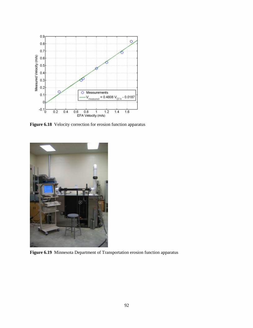
92

Figure 6.18 Velocity correction for erosion function apparatus

Figure 6.19 Minnesota Department of Transportation erosion function apparatus

93

6.5 Concluding Remarks

Twelve EFA tests were conducted by SDSU researchers. These included three thin wall tube samples

from the Big Sioux River Bridge (B-1 P-7, B-2 P-12, and B-2 P-14), five samples from the Split Rock

Creek bridges (B-4 P-2, B-5 P-10, B-5 P-12, B-6 P-6, and B-6 P-8), and four samples from the White

River Bridge (B-7 P-10, B-7 P-12, B-10 P-5, and B-10 P-7). Two additional thin wall tube soil samples

(B-9 P-1 and B-9 P-2) from duplicate soil locations at the White River Bridge were tested by TAMU to

assess the repeatability of the EFA tests conducted by SDSU. Duplicate samples were obtained by

drilling an adjacent drill hole approximately 5 lateral feet from drill hole B-7 and obtaining soil samples

at the same elevation as the adjacent samples (B-7 P-10 and B-7 P-12). All the samples were taken from

drill holes in the left or right abutments. Boring logs, bridge plans, and channel profile measurements

were studied to select the most probable representative samples for EFA testing. Of the 14 samples tested,

the results from eight tests (B-1 P-7, B-2 P-12, Big Sioux River site; B-4 P-2, B-5 P-10, Split Rock Creek

site; and B-9 P-1, B-9 P-2, B-10 P-5, P-10 P-7, White River site) were used with the SRICOS method to

predict the local scour depth at a total of five different bridge piers from the three study sites.

Several problems were encountered in the EFA tests. The flow velocity recorded by the EFA had to be

corrected. In addition, the stepping motor that operated the piston was underpowered. Thus, we had to use

an extruder to get rid of some soils from the thin wall tube before the remaining soils could be advanced

by the piston. This resulted in less soil available for EFA testing. During the test, the soil surface often

eroded non-uniformly so it was difficult to determine when the sample should be advanced from the tube.

It was also unsure what roughness height should be used to calculate the applied bed shear stress. When

the soil surface is eroding non-uniformly, vortices and eddies are formed in and around the scour holes so

the erosive action of the flowing water could be quite different from that in a simple shear flow.

Currently, there is no consensus on how the bed shear stress should be calculated in this situation. At

Texas A&M University, for example, the operator assesses the surface texture of the soil sample and

estimates the bed roughness as the soil erodes. This estimation is performed on all the flow velocities

tested. The process is inherently subjective, as it is unlikely that two different operators conducting

separate EFA tests on duplicate soil samples would produce the same results. Therefore, the procedure

was not used by SDSU researchers. For simplicity, a constant ε value was estimated by assessing the

texture of the eroding surface. This roughness height was applied to all the flow velocity tested. The

applied shear stress was also calculated for other ε values. These additional erosion-rate-versus-shear-

stress curves were used to determine the effects of critical shear stress and slope of the erosion rate curve

on the predicted final scour depths (see Sections 7, 8, and 9).

95

7. HYDRAULIC AND SCOUR ANALYSIS, BIG SIOUX RIVER BRIDGE 7.1 Site Description

A general description of the Big Sioux River Bridge can be found in Section 4. Additional site

information needed for hydraulic and scour analysis is included in this section.

Figure 7.1 shows a topographic map and an aerial photograph of the bridge site. As seen in Figure 7.1,

the Big Sioux River is a meandering stream. The river splits around a highland about 0.3 miles upstream

from the bridge crossing. On the downstream side of this highland, the re-combined channel flows south

and runs almost parallel to Highway 13, then sharply turns west and approaches the bridge crossing at a

large angle. Bridge crossing over or near a river bend would by itself produce non-uniform velocity

distribution across the channel. At this site, moreover, the left over bank in front of the bridge crossing

becomes submerged during moderate to high flows, so that flow in the south channel can cut across the

floodplain to approach the bridge crossing at a smaller angle. Because of the combined effect of channel

bend and exchange of flow between the main channel and floodplain, the flow angle of attack and

velocity distribution in the bridge opening can vary significantly with flow discharge.

Figures 7.2 through 7.7 show pictures of the bridge site taken during a field trip on April 6, 2007, when

the recorded daily mean flow was 1,968 ft3/s. It is important to note that there is a dam structure about

1/4 mile downstream of the bridge (see Figure 7.7). This dam maintains a minimum pool at the bridge

crossing during low flows. In addition, the water depth over the dam is at or close to critical depth during

low to moderate flows, when the dam is not submerged by tailwater.

Figure 7.8 shows the measured cross sections on the upstream and downstream faces of the bridge on four

different days in 1991-1993. The upstream cross section shows about 8.5 ft of local scour around the

northern-most pier (bent 2). At the downstream cross section, the scour hole was located on the left side

of the pier. There was an apparent flow concentration on the north side of the channel (see Figures 7.13

and 7.14). The upstream flow must approach the northern-most pier at an angle, which would account for

the location of the scour hole seen in the downstream cross section.

The Big Sioux River near Brookings streamflow gauging station (06480000) is located about 22 miles

upstream from the bridge site. This station has been operated since 1953. The estimated drainage areas at

the Brookings station and at the bridge site are 3,898 mi2 and 4,096 mi

2, respectively (Niehus 1996). To

model the river flow at the bridge, a drainage area adjustment ratio of 1.025 (= 3898/4096 ) was applied

to transfer the recorded discharges at the Brookings station to the bridge site. Between December 5,

1991, and July 7, 1993, the peak flow occurred on July 5, 1993, with a recorded daily mean flow of

11,583 ft3/s (Q2 = 2,320 ft

3/s) at the bridge site.

Figure 7.8 shows that most of the observed scour at the northern-most pier was developed between March

30 and July 7, 1993. This figure also shows a small amount (up to 1 ft) of contraction scour in the bridge

opening. Two borings (B-1 and B-2) were completed for this site. The data collected from the subsurface

explorations and the basic index and geotechnical engineering properties of the site soils are presented in

Section 5. The results of EFA tests are presented in Section 6. Borings B-1 P-7 and B-2 P-12 were

determined to be the most probable representative samples at the northern-most (bent 2) and southern-

most (bent 4) piers, respectively. The measured erosion rate versus shear stress curves for these two

samples (Figures 6.1 and 6.2) were used to predict the local scour at the two piers.

96

Figure 7.1 Topographic map (USGS, scale 1:24,000, 7/1/1978) and aerial photography (USGS,

9/8/1992) of bridge site, http://terraserver-usa.com

97

Figure 7.2 Bridge from left bank facing along upstream face toward right bank.

The piers in the channel are bent 4, 3, and 2 (from left to right).

Figure 7.3 From bridge facing upstream toward right bank

98

Figure 7.4 From bridge facing upstream toward tree island

Figure 7.5 From left bank facing upstream toward tree island

99

Figure 7.6 From bridge facing downstream

Figure 7.7 From 1/4 mile downstream facing upstream toward bridge site.

A dam is seen in the foreground.

100

Figure 7.8 Upstream and downstream cross sections at the Big Sioux River Bridge near Flandreau. The

ordinate for the upstream and downstream cross sections is the distance from the left

abutment and the abscissa is elevation above mean sea level, in feet (after Niehus 1996).

101

7.2 Hydraulic Modeling

Hydraulic analysis was conducted using the one-dimensional River Analysis System HEC-RAS. The

river system schematic used in the computation is shown in Figure 7.9. Five surveyed and three un-

surveyed cross sections were used in the HEC-RAS computation. The approach section (River Station

10) is located 1,060 ft (measured along the main channel) upstream of the bridge in the big bend of the re-

combined channel. The second cross section (River Station 9.5 Bridge Section Upstream) is located 5 ft

upstream of the bridge. The third cross section (River Section 9, Bridge Section Downstream) is located

5 ft downstream of the bridge. The exit section (River Station 7) is located 500 ft downstream from the

bridge. The fifth cross section (River Station 6, Weir Section Upstream) is located 5 ft upstream of the

dam or 745 ft downstream of River Station 7. The sixth cross section (River Station 5, Weir Section) is

located at the dam. The seventh cross section (River Station 4, Weir Section Downstream) is located 5 ft

downstream of the dam. The eighth cross section (Section 3, Downstream Section) is located 1,545 ft

downstream of River Station 4. Cross sections 9.5 and 9 were taken from the river bottom profile survey

on the upstream and downstream faces of the bridge on June 22, 1992, before the scour hole developed at

the northern-most pier. HEC-RAS superimposes the bridge geometry onto cross sections 9.5 and 9 to

form the cross sections inside the bridge at the upstream and downstream ends. Initially, one additional

cross section (River Station 8) was interpolated from cross sections 9 and 7 and placed between these two

cross sections to define the ineffective flow areas downstream of the bridge. The addition of this cross

section had no effects on the computed results and thus it was deleted. Manning coefficient was selected

following the following guidelines: 0.03 (clean and straight channel), 0.035 (pasture and farmland), 0.05

(light brush), 0.075 (heavy brush), and 0.15 (trees).

For the bridge geometry, the width of the bridge deck is 32.33 ft. The pier centerline stations are 98 (bent

4), 219 (bent 3) and 338 (bent 2) ft from the left abutment (Niehus 1996). The width of the piers is 3 ft

and the length is 30 ft. The upstream and downstream embankment side slope is 3 horizontal to 1 vertical.

The high chord and low chord elevations were estimated from the bridge drawings and entered into HEC-

RAS. However, their values had no effects on the computed results since the road was not overtopped in

1991-1993.

The Energy (Standard Step) method was used to compute the flow through the bridge, categorized as

class A low flow (sub-critical flow with water surface below the low chord). Water surface elevation was

not measured at the downstream cross section (River Station 3). Therefore, a range of values including

the normal depth were tried. Table 7.1 shows the computed results for a discharge of 9,090 ft3/s. This

discharge was recorded at the bridge site on March 30, 1993, by the USGS using standard stream gauging

techniques. Three different water surface profiles (PF1, PF2, PF3) are computed for three different water

surface elevations (1,529, 1,529.5, and 1,530 ft) prescribed downstream at River Station 3. For reference,

the water surface elevation corresponding to the normal depth (average downstream slope = 0.000324) is

1,529.31 ft. The Froude number shown in the last column of the table shows that flow over the dam is

critical for PF1 and sub-critical for PF2 and PF3. Below 1,529 ft, the flow over the dam is critical and

water surface elevation downstream of the dam has no effects on the hydraulics at the bridge. Above

1,529 ft, the dam becomes submerged but the effect of downstream water level on the hydraulics at the

bridge is very small (see W.S. Elevation, River Station 9.5, Table 7.1). This analysis was repeated for

other discharges. It was found that, for the range of flow discharges (100 to 12,000 ft3/s) considered in

this study, the water level downstream of the dam had little or no effects on the water surface elevation

and flow velocity at the bridge unless the downstream water level was set substantially higher than the

normal depth.

102

Flandreau

10

9.59

7

6

3

Big

Si oux Ri ve r

Figure 7.9 River schematic used in HEC-RAS computation

0 1000 2000 3000 40001510

1515

1520

1525

1530

1535

1540

1545

1550

Main Channel Distance (ft)

Ele

va

tio

n (

ft)

Legend

EG PF 1

WS PF 1

Crit PF 1

Ground

Big Sioux River Flandreau

Figure 7.10 Computed water surface profile at Big Sioux River Bridge for flow discharge of 9,090 ft

3/s.

The water depth downstream is normal depth.

103

An example of the computed water surface profile is shown in Figure 7.10. The minimum channel

elevation is 1515.72 ft at River Station 9.5 (Bridge Section Upstream) and 1511.12 ft at River Station 9

(Bridge Section Downstream). These elevations are considerably lower than the bed elevation upstream

and downstream (see Min Ch Elevation, Table 7.1). The lower bed elevation at the bridge is due only in

part to the scour hole (see Figure 7.8). The surveyed cross sections showed that the bed elevation at the

bridge crossing was indeed much lower than the bed elevation upstream and downstream.

Table 7.2 shows a comparison of the measured and computed water surface elevations on the upstream

side of the bridge on four days when discharge and water level were measured at the bridge site by the

USGS. This table shows that the measured and computed water surface elevations are reasonably close.

We found that the computed water surface elevation at the bridge was very sensitive to the crest length

and elevation of the dam. The dam had been surveyed by the USGS in 1991-1993, and again by us in the

fall of 2007. Our own survey showed that the dam was 175 ft wide instead of the 165 ft reported by the

USGS. However, we were unable to measure the crest elevation of the dam in the swift water. In the

HEC-RAS computations, we had used a crest elevation of 1,524.30 ft for the dam. This elevation was

lower than the elevation of 1,524.97 ft surveyed by the USGS. We had to reduce the elevation of the dam

from 1,524.97 to 1,524.30 ft in order to match the predicted and measured water surface elevations at the

bridge. Note that all channel profile measurements used in the hydraulic and scour analyses were taken

from the USGS field survey in 1991 to 1993 unless stated otherwise.

Table 7.1 HEC-RAS results for flow discharge of 9,090 ft3/s

River

Station Profile

Min Ch

Elevation

W.S.

Elevation

Critical

W.S.

Velocity

Chl

Flow

Area

Top

Width

Froude

# Chl

(ft) (ft) (ft) (ft/s) (sq ft) (ft)

10 PF 1 1523.07 1530.87 1.56 6714.18 1414.02 0.1

10 PF 2 1523.07 1530.88 1.56 6724.54 1414.45 0.1

10 PF 3 1523.07 1531.06 1.51 6976.35 1424.96 0.1

9.5 PF 1 1515.72 1530.68 1522.88 2.71 3353.33 341.54 0.15

9.5 PF 2 1515.72 1530.69 1522.88 2.71 3355.96 341.59 0.15

9.5 PF 3 1515.72 1530.88 1522.88 2.66 3420.07 342.75 0.15

9.25 Bridge

9 PF 1 1511.12 1530.67 2.7 3361.91 344.81 0.15

9 PF 2 1511.12 1530.68 2.7 3364.6 344.84 0.15

9 PF 3 1511.12 1530.87 2.65 3429.52 345.78 0.15

7 PF 1 1520.77 1530.59 2.78 4549.19 1020.33 0.17

7 PF 2 1520.77 1530.6 2.77 4557.66 1020.35 0.17

7 PF 3 1520.77 1530.8 2.66 4758.86 1020.89 0.16

6 PF 1 1520.5 1530.42 2.77 3853.43 1318.85 0.18

6 PF 2 1520.5 1530.43 2.76 3865.51 1318.87 0.18

6 PF 3 1520.5 1530.64 2.64 4151.8 1319.28 0.17

5 PF 1 1524.3 1528.54 1528.54 10.81 840.88 232.57 1

5 PF 2 1524.3 1528.99 1528.54 9.57 950.03 262.27 0.89

5 PF 3 1524.3 1529.7 1528.54 7.84 1189.27 1222.7 0.72

104

(Table 7.1 continued)

4 PF 1 1520.5 1529.49 3.25 2795.67 404.48 0.22

4 PF 2 1520.5 1529.87 3.06 3138.26 1317.82 0.2

4 PF 3 1520.5 1530.28 2.84 3676.2 1318.59 0.18

3 PF 1 1520 1529 1523.87 2.1 4319.5 1091 0.19

3 PF 2 1520 1529.5 1523.87 1.86 4887.38 1180.5 0.16

3 PF 3 1520 1530 1523.87 1.65 5500 1270 0.14

Table 7.2 Comparison of measured and computed water surface elevations on upstream face of bridge.

The discharges were measured by standard stream gauging techniques using a Price AA type

current meter.

Date Q (ft3/s)

WSEL (ft)

(Measured)

WSEL (ft)

(HEC-RAS)

6/20/1992 1,624 1,526.54 1,526.51

6/22/1992 4,346 1,528.82 1,528.36

3/30/1993 9,090 1,530.42 1,530.68

7/7/1993 7,774 1,530.15 1,530.12

-600 -400 -200 0 200 400 600 800 1000 12001522

1524

1526

1528

1530

1532

1534

1536

1538

1540

Approach Section

Station (ft)

Ele

va

tion (

ft)

Legend

EG PF 1

WS PF 1

0.0 ft/s

0.5 ft/s

1.0 ft/s

1.5 ft/s

2.0 ft/s

Ground

Bank Sta

.035 .03

Figure 7.11 Approach section in HEC-RAS. The computed water surface elevation

and velocity distribution are for a discharge of 9,090 ft3/s.

105

0 100 200 300 400 5001515

1520

1525

1530

1535

1540

1545

Bridge Section Upstream

Station (ft)

Ele

va

tion (

ft)

Legend

EG PF 1

WS PF 1

Crit PF 1

0 ft/s

1 ft/s

2 ft/s

3 ft/s

4 ft/s

Ground

Bank Sta

.03

Figure 7.12 Bridge section upstream. The computed water surface elevation

and velocity distribution are for a discharge of 9,090 ft3/s.

Figures 7.11 and 7.12 show the measured ground elevation, computed water surface elevation, and

computed flow velocity distribution at the approach section and on the upstream face of bridge for a

discharge of 9,090 ft3/s. The entire cross section has been subdivided into 40 stream tubes to calculate the

velocity distribution. There are 20 vertical slices in the main channel and 10 each in the left and right

over bank. In the approach section, the depth-averaged velocity in the main channel is nearly uniform at

around 1.7 ft/s. The depth-averaged velocity in the left over bank is less than 1 ft/s. In the upstream

bridge cross section, depth-averaged velocity varies across the channel with the highest velocity (about

3.4 ft/s) found in the deepest part of the channel (between stations 220 and 280).

Figures 7.13 and 7.14 show a comparison of the measured and computed velocity distributions on the

upstream face of the bridge for March 30 and July 7, 1993. Note that the area under the measured

distribution is larger than the area under the computed distribution. In these figures, the measured

velocity is the flow velocity in the direction of the approach flow, which is not necessarily perpendicular

to the bridge. On March 30, 1993, the measured flow angle of attack was about 30 degrees at the

northern-most pier (bent 2), 20 degrees at the center pier (bent 3) and 0 degrees at the southern-most pier

(bent 4). The one-dimensional river analysis model HEC-RAS predicts the flow velocity at bent 4 and 3

(station 98 and 219 ft) well, but under-predicts the velocity at bent 2 (station 338 ft) by almost a factor of

2 (Figure 7.13). The measured velocity reaches a peak of 5.2 ft/s at station 325, then decreases sharply to

0.64 ft/s at station 370, some 30 ft away from the right bank (station 400). Figure 7.14 shows the

comparison for July 7, 1993 (Q = 7,774 ft3/s). The measured flow angle of attack was larger for the

smaller discharge; it was approximately 40 degrees at bent 2, 34 degrees at bent 3, and 11 degrees at bent

4. In addition, the location of maximum measured velocity (4.78 ft/s) has shifted from bent 2 towards the

middle of the channel where bent 3 is located. We believe that the flow concentration on the north side of

the channel is a two-dimensional effect caused by the sharp turn of the river around the right abutment.

We speculate that the flow angle of attack decreases during moderate to high flows because a portion of

the discharge can overtop the high ground in front of the bridge to approach the bridge crossing at a

smaller angle.

106

Figure 7.13 Comparison of measured and computed flow velocities on upstream face of bridge for

March 30, 1993. The pier sets are at 98 (bent 4), 219 (bent 3), and 338 (bent 2) ft from the

left abutment.

Figure 7.14 Comparison of measured and computed flow velocities on upstream face of bridge for July

7, 1993. The pier sets are at 98 (bent 4), 219 (bent 3), and 338 (bent 2) ft from the left

abutment.

107

Figure 7.15 Rating curve for computed water surface elevation on upstream face

of Big Sioux River Bridge

The two-dimensional flow effect described above cannot be predicted by a one-dimensional model such

as HEC-RAS. A numerical study using the Surface Water Modeling System (SMS) is currently underway

to investigate two-dimensional flow effects at the Big Sioux River site. For the present bridge scour

study, a correction factor was applied to the computed flow velocities by HEC-RAS in order to predict the

local scour at bent 2. Since high flow should produce most of the observed scour, the correction factor

was chosen to be 1.8 (ratio of measured and computed velocities at Q = 9,090 ft3/s).

Figure 7.15 shows the rating curve for the computed water surface elevation on the upstream face of the

bridge. For reference, the measured channel elevations at bent 2 and bent 4 on June 22, 1992, were

1,520.72 and 1,522.92 ft, respectively. Note that the dam maintained a minimum pool at the bridge site

during low to moderate flows.

Figures 7.16 and 7.17 show the rating curves for the computed flow velocities at bent 2 and bent 4. The

computed velocities were computed using HEC-RAS and do not include the effects of flow angle of

attack and flow concentration on the north side of the channel. The moderate flow velocities are the

results of large water depths at the bridge crossing.

108

Figure 7.16 Rating curve for computed approach flow velocity at bent 2

Figure 7.17 Rating curve for computed approach flow velocity at bent 4

109

7.3 Erosion Rate versus Shear Stress Curves

The erosion rate curves used for scour prediction at the Big Sioux River Bridge are Figures 6.1 (boring B-

1 P-7) and 6.2 (boring B-2 P-12). Boring B-1 P-7 (very silty fine sand) was collected from the right

(north) abutment at an elevation close to the initial bed elevation at the northern-most pier. Figure 6.1

was used with the SRICOS method to compute the pier scour at bent 2. Boring B-2 P-12 (organic silt

with abundant organic fibers) was collected from the left (south) abutment at an elevation close to the

initial bed elevation at the southern-most pier. Figure 6.2 was used to compute the pier scour at bent 4. In

each figure, the measured soil erosion rates had been fitted with a straight line for the applied bed shear

stress calculated using four different values of bed roughness height ( = 0, 1, 2, and 3 mm). In the EFA

tests, a roughness height was estimated and used to calculate the applied bed shear stress. To assess the

effect of uncertainty in the calculated bed shear stress on the predicted scour depth, scour predictions

were first conducted using one of the four erosion rate curves ( = 0, 1, 2, or 3 mm). These results formed

the baseline case, with which the results from the other cases were compared. Scour predictions were

also conducted for a range of values of critical shear stress and slope of erosion rate versus shear stress

curve to examine the sensitivity of the predicted scour depth to these parameters.

7.4 Scour Measurements

Measured cross sections on the upstream side of the Big Sioux River Bridge are available on June 20 and

June 22, 1992, and on March 30 and July 7, 1993 (see Figure 7.8). These profiles show about 8.5 ft of

pier scour at bent 2. The large scour depth at bent 2 is consistent with the high soil erosion rates seen in

Figure 6.1 and the observed flow concentration on the north side of the channel. There is up to 1 ft of

total scour at bent 4, most of which appears to be contraction scour. The much lesser scour at bent 4 is

consistent with the slower soil erosion rates seen in Figure 6.2 and the smaller flow velocities on the south

side of the channel (see Figures 7.13 and 7.14).

7.5 Flow Histories

The Big Sioux River near Brookings streamflow gauging station (06480000) is located about 22 miles

upstream from the bridge site. Figure 7.18 shows the recorded daily mean flow and hourly mean flow

from the Brookings station for 1992 and 1993. Two large floods (maximum recorded hourly mean flow

9,530 ft3/s and 13,300 ft

3/s) on June 21 and July 4, 1993, dominate the hydrograph of this period. For

comparison, the estimated 2-year, 100-year and 500-year discharges at the Brookings station are 2,320,

31,300, and 53,100 ft3/s, respectively (Niehus 1996).

110

Figure 7.18 Hydrographs from Big Sioux River near Brookings streamflow gauging station. The upper

plot is the daily mean flow from June 22, 1992, to July 7, 1993. The lower plot is the hourly

mean flow from March 28, 1993, to July 7, 1993. The measured discharges shown were

multiplied by 1.025 in the SRICOS simulation to account for the increase in drainage area

between the Brookings station and the bridge site.

7.6 Scour Predictions A program for computing pier and contraction scour using the SRICOS method can be downloaded from

a website maintained by Professor Jean-Louis Briaud at Texas A&M University

(http://ceprofs.tamu.edu/briaud/SRICOS-EFA.htm). We have also written our own FORTRAN codes

based on the scour equations and methodology documented in NCHRP Report 516 (Briaud et al. 2004a).

Our computer codes differ from Dr. Briaud’s program in how the correction factors for flow depth, flow

angle of attack, and pier spacing are applied; this is discussed in Section 2. The scour predictions

presented in this report were obtained using our own computer codes. The values of the input parameters

for the baseline case are given in Table 7.3.

111

Table 7.3 Summary of input parameters for scour predictions in the baseline case

Pier geometry: Pier width B = 3 ft, pier length L = 30 ft, pier shape rectangular pier with round

nose

Channel geometry: Channel upstream width W1 = 436 ft, number of piers N = 3, pier spacing S =

120 ft, initial bed elevation Y0 = 1520.72 ft (bent 2) and 1522.92 (bent 4)

Flow parameters: Flow angle of attack = 25 degrees (bent 2), and 0 degrees (bent 4)

Fluid parameters: Density = 998.2 kg/m3, kinematic viscosity ν = 1.004 10

-6 m

2/s

Soil parameters: Bent 2: critical shear stress τc = 18.59 N/m2, slope of erosion rate curve C1 = 7.49

mm/hr/(N/m2) (corresponding to ε = 1.0 mm)

Bent 4: critical shear stress τc = 25.35 N/m2, slope of erosion rate curve C1 = 3.12

mm/hr/(N/m2) (corresponding to ε = 1.0 mm)

Hydrograph: Time step Δt = 24 hours (daily mean flow) and 1 hour (hourly mean flow),

number of time steps M = 381 (daily mean flow; June 22, 1992 through July 7,

1993) and 2,640 (hourly mean flow; March 28, 1993 through July 7, 1993).

In the SRICOS simulations, the flow discharges shown in Figure 7.18 were multiplied by 1.025 to

account for the increase in drainage area between the Brookings station and the bridge site. As seen in

Figure 7.18, the hydrograph in 1992-1993 was dominated by two large floods on June 21 and July 4,

1993. The observed flow angle of attack at bent 2 for Q = 9,090 ft3/s was about 30 degrees. The hourly

mean flow exceeded 9,000 ft3/s all day on June 20 and July 5, and for part of the day on June 19, June 21,

July 4, and July 6. We expect the flow angle of attack to be less than 30 degrees during high flows, since

the headland on the left bank in front of the bridge would be submerged. Therefore, a flow angle of

attack of 25 degrees was assumed in predicting the pier scour at bent 2. Finally, the computed approach

flow velocity at bent 2 from HEC-RAS (Figure 7.16) was multiplied by 1.8 to account for the observed

flow concentration on the north side of the channel.

Figure 7.19 shows the SRICOS simulation at bent 2 from June 22, 1992, through July 7, 1993, based on

the recorded daily mean flow. From top to bottom, the plots show the time history of flow discharge Q,

approach flow velocity V1, approach flow depth y1, initial bed shear stress τ, initial rate of scour dz/dt,

maximum (equilibrium) scour depth zmax, and predicted scour depth z. The critical shear stress τc for the

soil is shown as a dashed line in the initial bed shear stress plot. Figure 7.19 shows that the critical shear

stress was exceeded for only a few days between June 20 and July 6, 1993. The entire predicted scour

occurs during these few days. The predicted final scour depth on July 7, 1993, is 9.17 ft.

112

Figure 7.19 SRICOS simulation for bent 2, June 22, 1992, through July 7, 1993; baseline conditions.

The discharge is daily mean flow. The critical shear stress τc is shown as a dashed line in

the initial bed shear stress plot.

113

Figure 7.20 SRICOS simulation for bent 2, March 28 to July 7, 1993; baseline conditions.

The discharge is hourly mean flow.

114

Figure 7.21 SRICOS simulation for bent 4, March 28 to July 7, 1993; baseline conditions.

The discharge is hourly mean flow.

115

Figure 7.20 shows the SRICOS simulation for bent 2 from March 28 through July 7, 1993, based on the

recorded hourly mean flow. The results are qualitatively similar to those shown in Figure 7.19 but the

computed scour depths are slightly larger. The predicted final scour depth on July 7, 1993, is 9.54 ft.

Hence, using smaller time steps do increase the predicted scour, at least for the flow conditions at this

site. Figure 7.20 also shows that a small amount of scour (about 0.2 ft) occurs between March 30 and

June 21. Both Figures 7.19 and 7.20 predict that no scour occurs before March 30, which is in general

agreement with the measured cross sections shown in Figure 7.8. The predicted final scour depths are

reasonably close to the observed scour depth of about 8.5 ft.

Figure 7.21 shows the results of SRICOS simulation for bent 4. For bent 4, the flow angle of attack was

assumed to be zero and the computed approach flow velocity from HEC-RAS was used without any

corrections. The SRICOS method predicts no scour. As seen in Figure 7.21, the initial bed shear stress

never exceeds the critical shear stress of 25.35 N/m2 (not plotted). Note that the predicted scour depth

will still be zero if the erosion rate versus shear stress curve for ε = 0 is used, which will lower the critical

shear stress to 9.4 N/m2. The latter is shown as a dashed line in the initial bed shear stress plot. The

lesser critical shear stress is still larger than the initial bed shear stress at all time steps.

7.7 Sensitivity Analysis

There are many uncertainties associated with the SRICOS simulations at this site. The main uncertainties

in flow parameters include the approach flow velocity and flow angle of attack. The main uncertainties in

the soil parameters include the critical shear stress and slope of the erosion rate versus shear stress curve.

The effects of these uncertainties on the predicted final scour depth are discussed below. The sensitivity

analysis was conducted for bent 2 using the hourly mean flow.

Figures 7.22 and 7.23 show the effects of flow angle of attack and approach flow velocity on the

predicted final scour depth at bent 2. As discussed earlier, we expect that the flow angle of attack for the

two floods on June 21 and July 4, 1993, to be less than 30 degrees, but the exact amount is unknown.

Figure 7.22 shows that reducing the flow angle of attack from 25 degrees to 19 degrees would reduce the

predicted final scour depth from 9.54 ft to 8.17 ft. The latter is close to the observed scour. However, the

effect of approach flow velocity is much greater. This is because the bed shear stress is proportional to the

velocity squared (see Equation 2.11). Figure 7.23 shows that reducing the velocity multiplying factor

from 1.8 to 1.7 will reduce the predicted final scour depth from 9.54 ft to 8.16 ft. The velocity

multiplying factor was applied to account for the flow concentration observed near the right abutment.

This phenomenon is a two-dimensional effect which cannot be predicted by a one-dimensional model

such as HEC-RAS. Figures 7.22 and 7.23 show that the difference between the predicted and observed

scour depths is within the uncertainty limits in the flow angle of attack and approach flow velocity.

The applied bed shear stress in the EFA test could not be determined precisely since the effective

roughness height was unknown. Therefore, erosion rate versus shear stress curves were prepared for four

different values of roughness height (ε = 0, 1, 2, and 3 mm) (see Figure 6.1). The corresponding critical

shear stress ranges from 7.2 to 28.8 N/m2, and the slope of the erosion rate versus shear stress curve

ranges from 23.45 to 4.82 mm/hr/(N/m2). In the SRICOS simulations, we had used the erosion rate

versus shear stress curve for ε = 1 mm to predict the soil erosion rates. During the EFA test, the soil was

advanced 1 mm into the flow one at a time. The soil eroded quickly particle by particle more or less

uniformly. For these test conditions, a roughness height of 2 or 3 mm would probably be too high. On

the other hand, the eroding surface was not entirely smooth. Hence, a roughness height of 1 mm was

considered a reasonable choice. Using these results as the baseline case, we then examined the sensitivity

of the predicted final scour depth to the critical shear stress and slope of the erosion rate versus shear

stress curve.

116

Figure 7.22 Effect of flow angle of attack on predicted final scour depth at bent 2

Figure 7.23 Effect of approach flow velocity on predicted final scour depth at bent 2

117

We note that the predicted scour history shown in Figure 7.20 is consistent with field measurements. It

shows that most of the predicted scour is produced by the two largest floods on June 21 and July 4, 1993.

If the erosion rate versus shear stress curve for ε = 0 is used, the predicted final scour depth will be 13.37

ft, which is much larger than the observed scour. Those results will also show that 9.4 ft of scour is

developed between March 30 and June 21, before the two largest floods arrived. If the erosion rate versus

shear stress curves for ε = 2 and 3 mm are used to predict scour, the predicted final scour depth will be

5.54 and 2.62 ft, respectively. These scour depths are much smaller than the observed scour depth.

To examine the effect of critical shear stress on the predicted final scour depth, we keep all the other input

parameters fixed and vary the critical shear stress from 7.0 to 30.5 N/m2. The results are shown in Figure

7.24. Note that the critical shear stress has a significant effect on the predicted final scour depth. For

example, increasing the critical shear stress from 18.6 N/m2 (corresponding to ε = 1 mm) to 21.5 N/m

2

(corresponding to ε = 1.3 mm) will reduce the predicted final scour depth from 9.54 to 8.25 ft. In

practice, it will be difficult to estimate the bed roughness height in an EFA test to within ±0.5 mm.

Figure 7.20 shows that the maximum equilibrium scour depth is not reached during the two largest floods

on June 21 and July 4. Hence, the slope of the erosion rate versus shear stress curve will also have an

effect on the predicted final scour depth. In Figure 7.25, we vary the slope of the erosion rate versus

shear stress curve but keep the other input parameters the same as in the baseline case. For comparison

purposes, the slopes of the erosion rate versus shear stress curve for ε = 0, 1, and 2 mm are 23.45, 7.49,

and 5.74 mm/hr/(N/m2), respectively. As the roughness height increases, the slope decreases. Figure

7.25 shows that reducing the slope from 7.49 to 5.5 mm/hr/(N/m2) will reduce the predicted final scour

depth from 9.54 to 8.53 ft. If the critical shear stress is kept constant, the slope of the erosion rate versus

shear stress curve can only be reduced by increasing the value of ε when calculating the applied bed shear

stress for those flow velocities that are above the threshold velocity for initiation of soil erosion. For a

critical shear stress of 18.6 N/m2, the ε value needed to produce a slope of 5.5 mm/hr/(N/m

2) for the

erosion rate versus shear stress curve will be approximately 1.4 mm, assuming that the same roughness

height is used for all flow velocities above the threshold velocity.

Figures 7.24 and 7.25 show that the predicted final scour depth is very sensitive to the critical shear stress

and the slope of the erosion rate versus shear stress. Between the two, the critical shear stress is the more

important parameter. Thus, having accurate information on the approach flow velocity and critical shear

stress would be critical to reliable scour predictions at this site.

118

Figure 7.24 Effect of critical shear stress on predicted final scour depth at bent 2

Figure 7.25 Effect of slope of erosion rate curve on predicted final scour depth at bent 2

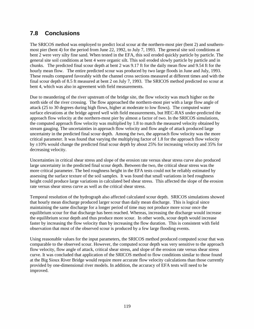
119

7.8 Conclusions

The SRICOS method was employed to predict local scour at the northern-most pier (bent 2) and southern-

most pier (bent 4) for the period from June 22, 1992, to July 7, 1993. The general site soil conditions at

bent 2 were very silty fine sand. When tested in the EFA, this soil eroded quickly particle by particle. The

general site soil conditions at bent 4 were organic silt. This soil eroded slowly particle by particle and in

chunks. The predicted final scour depth at bent 2 was 9.17 ft for the daily mean flow and 9.54 ft for the

hourly mean flow. The entire predicted scour was produced by two large floods in June and July, 1993.

These results compared favorably with the channel cross sections measured at different times and with the

final scour depth of 8.5 ft measured at bent 2 on July 7, 1993. The SRICOS method predicted no scour at

bent 4, which was also in agreement with field measurements.

Due to meandering of the river upstream of the bridge site, the flow velocity was much higher on the

north side of the river crossing. The flow approached the northern-most pier with a large flow angle of

attack (25 to 30 degrees during high flows, higher at moderate to low flows). The computed water

surface elevations at the bridge agreed well with field measurements, but HEC-RAS under-predicted the

approach flow velocity at the northern-most pier by almost a factor of two. In the SRICOS simulations,

the computed approach flow velocity was multiplied by 1.8 to match the measured velocity obtained by

stream gauging. The uncertainties in approach flow velocity and flow angle of attack produced large

uncertainty in the predicted final scour depth. Among the two, the approach flow velocity was the more

critical parameter. It was found that varying the multiplying factor of 1.8 for the approach flow velocity

by ±10% would change the predicted final scour depth by about 25% for increasing velocity and 35% for

decreasing velocity.

Uncertainties in critical shear stress and slope of the erosion rate versus shear stress curve also produced

large uncertainty in the predicted final scour depth. Between the two, the critical shear stress was the

more critical parameter. The bed roughness height in the EFA tests could not be reliably estimated by

assessing the surface texture of the soil samples. It was found that small variations in bed roughness

height could produce large variations in calculated bed shear stress. This affected the slope of the erosion

rate versus shear stress curve as well as the critical shear stress.

Temporal resolution of the hydrograph also affected calculated scour depth. SRICOS simulations showed

that hourly mean discharge produced larger scour than daily mean discharge. This is logical since

maintaining the same discharge for a longer period of time may not produce more scour once the

equilibrium scour for that discharge has been reached. Whereas, increasing the discharge would increase

the equilibrium scour depth and thus produce more scour. In other words, scour depth would increase

faster by increasing the flow velocity than by increasing the flow duration. This is consistent with field

observation that most of the observed scour is produced by a few large flooding events.

Using reasonable values for the input parameters, the SRICOS method produced computed scour that was

comparable to the observed scour. However, the computed scour depth was very sensitive to the approach

flow velocity, flow angle of attack, critical shear stress, and slope of the erosion rate versus shear stress

curve. It was concluded that application of the SRICOS method to flow conditions similar to those found

at the Big Sioux River Bridge would require more accurate flow velocity calculations than those currently

provided by one-dimensional river models. In addition, the accuracy of EFA tests will need to be

improved.

121

8. HYDRAULIC AND SCOUR ANALYSIS, SPLIT ROCK CREEK BRIDGES

8.1 Site Description

A general description of the Split Rock Creek bridges can be found in Section 2. Additional site

information needed for hydraulic and scour analysis is included in this section.

Figure 8.1 Topographic map (USGS, scale 1:24,000, 7/1/1978) of bridge site

(http://terraserver-usa.com)

Bridge Site

122

Figure 8.2 Aerial photograph (USGS, 10/12/1991) of bridge site (http://terraserver-usa.com)

Figures 8.1 and 8.2 show a topographic map and an aerial photograph of the bridge site. Figures 8.3

through 8.6 show pictures of the bridge site taken during a field trip on April 9, 2007, when the recorded

daily mean flow was 232 ft3/s. As seen in these photographs, the banks are covered with grass and weeds,

and the floodplain cover is mainly crops, grass, and small trees. There is a large bend in the river a few

hundred feet upstream from the westbound bridge. This bend appears to be stable, and the channel

through the bridge openings had not shifted over time. The floodplain upstream and downstream is much

wider (about 2,000 ft wide) than the bridge openings. However, HEC-RAS predicts that at a discharge of

18,900 ft3/s, which was the peak flow recorded on May 8, 1993, the river would still be confined within

the main channel. These calculations also show that the width of the water surface in the cross section

about 500 ft upstream from the westbound bridge is about the same as that at the bridge opening.

Therefore, there was probably not a great deal of flow contraction at the bridge crossings during the flood

in May 1993.

Bridge Site

123

Figure 8.3 Picture of river from left bank facing upstream of the westbound bridge

Figure 8.4 Picture of bridge from left bank facing downstream face of the westbound bridge. Bent 3 is

the pier set in the low-flow channel. The two adjacent pier sets are bent 2 (right bank) and

bent 4 (left bank).

124

Figure 8.5 Picture of bridge from left bank facing upstream face of eastbound bridge

Figure 8.6 Picture of river from left bank facing downstream of eastbound bridge

125

Figure 8.7 Upstream and downstream cross sections at the Split Rock Creek bridges near Brandon. The

ordinate is distance from the left abutment and the abscissa is elevation above mean sea level,

in feet (after Niehus 1996). At both bridges, the largest scour depth was found around bent 3

in the main channel.

126

Figure 8.7 shows the measured channel cross sections on the upstream side of the westbound bridge and

on the downstream side of the eastbound bridge in 1991-1993. At both bridges, the largest scour was

found around bent 3 in the main channel. The maximum scour depth was 2 to 3 ft at the westbound

bridge and about 4 ft at the eastbound bridge. Most of the scouring was developed between March 29 and

May 8, 1993. The amount of contraction scour appears to be small (less than 1 ft). There was some

channel erosion and deposition at both bridges.

A gauging station (06482610) is located less than 1 mile upstream of the bridge sites, but it operated only

as a crest-stage partial-record gauging station from 1990 through 1993. The largest recorded peak

discharge at this gauging station in 1992-1993 was 18,900 ft3/s on May 8, 1993. The estimated drainage

areas at the gauging station and at the bridge sites are 464 mi2 and 466 mi

2, respectively (Niehus 1996).

The estimated 2-year, 100-year, and 500-year discharges at the bridge sites are 2,200, 22,500, and 39,200

ft3/s, respectively (Niehus 1996).

Four borings (B-3 to B-6) were completed at this site. The data collected from the subsurface


Section 5. The results of EFA tests are presented in Section 6. Boring B-4 P-2 from the left abutment and

boring B-5 P-10 from the right abutment were determined to be the most probable representative samples

for the foundation soil at the main channel pier (bent 3). The measured erosion rate versus shear

stress curves for these samples (Figures 6.4 and 6.5) were used to predict the pier scour depth at bent 3.


Hydraulic analysis was performed using HEC-RAS. The river system schematic used in the computation

is shown in Figure 8.8. Eight surveyed and one un-surveyed cross sections were used in the HEC-RAS

computation. River Stations 0, 1, and 2 are located 1,560 ft, 900 ft, and 455 ft, respectively, downstream

from the eastbound bridge. River Stations 3 and 3.4 are located 5 ft on either sides of the eastbound

bridge; their channel cross sections were taken from the surveyed cross section at the eastbound bridge on

December 6, 1991. River Stations 3.6 and 4 are located 5 ft on either sides of the westbound bridge; their

cross sections were taken from the surveyed cross section at the westbound bridge on March 29, 1993.

Stations 5, 6, 7 and 8 are located 492 ft, 1,022 ft, 2,692 ft, and 4,612 ft, respectively, upstream from the

westbound bridge. HEC-RAS superimposes the eastbound bridge geometry onto cross sections 3 and 3.4,

and the westbound bridge geometry onto cross sections 3.6 and 4 to form the cross sections inside the

bridges at their respective upstream and downstream ends. Manning coefficient was selected following

the following guidelines: 0.03 (clean and straight channel), 0.035 (pasture and farmland), 0.05 (light

brush), 0.075 (heavy brush), and 0.15 (trees).

The eastbound and westbound bridges were modeled as two separate parallel bridges. For both bridges,

the width of the bridge deck is 30.0 ft, and the channel distance between the bridge centerlines is 82 ft.

The pier centerline stations are 47 ft (bent 5), 97 ft (bent 4), 167 ft (bent 3), and 256 ft (bent 2) from the

left abutment at the eastbound bridge, and 53 ft (bent 5), 105 ft (bent 4), 175 ft (bent 3), and 264 ft (bent

2) from the left abutment at the westbound bridge. The width of the piers ranges from 2.75 to 3.0 ft. The

upstream and downstream embankment side slope is 2 horizontal to 1 vertical. The high chord and low

chord elevations were estimated from the bridge drawings and entered into the program. However, their

values had no effects on the computed results since the roadway was not overtopped.

The Energy (Standard Step) method was used to compute flow through the bridges, categorized as class A

low flow (sub-critical flow with water surface below the low chord). The stage-discharge relationship at

the downstream cross section (River Station 0) is unknown. Therefore, uniform flow was assumed at

Station 0 together with an average downstream slope of 0.00056. Table 8.1 shows the computed results

127

for a discharge of 14,700 ft3/s. This discharge was measured at the bridge site on May 8, 1993, by the

USGS using standard stream gauging techniques. Three different water surface profiles (PF1, PF2, PF3)

are computed for three different water surface elevations (1,317, 1,318.19, and 1,519 ft) prescribed

downstream at River Station 0. The water surface elevation of 1,318.19 ft corresponds to the normal

depth. These results show that the downstream water depth has some effects (around 5% for the flow

conditions shown) on the computed water depths and flow velocities at the bridges (see River Stations 3

and 4). This may be expected since the reach length between the eastbound bridge and River Station 0 is

only 1,560 ft. A sensitivity analysis was conducted to evaluate the effects of water depth and flow

velocity on the computed scour depth; this will be discussed. Figure 8.9 shows the computed water

surface profile for a flow discharge of 14,700 ft3/s and normal depth specified at River Station 0.


and downstream sides of the bridges on three different days when discharge and water level were

measured at the bridge site by the USGS. This table shows that the measured and computed water surface

elevations are reasonably close when uniform depth was specified downstream.

Reach 1

8

7 6

5

43

2

1

0

Sp

lit

Rock C r eek


Westbound Bridge

Eastbound Bridge

128

Table 8.1 HEC-RAS results for flow discharge of 14,700 ft3/s

River

Station Profile

Min Ch

El

W.S.

Elev

Crit

W.S.

Vel

Chnl

Flow

Area

Top

Width

Froude

# Chl

(ft) (ft) (ft) (ft/s) (sq ft) (ft)

8 PF 1 1303.52 1319.95 4.71 3836.42 1047.31 0.26

8 PF 2 1303.52 1320.39 4.32 4299.53 1064.85 0.23

8 PF 3 1303.52 1320.79 4 4723.89 1075.76 0.21

7 PF 1 1301.92 1319.44 3.24 5409.04 954.78 0.18

7 PF 2 1301.92 1319.98 2.97 5938.9 1000.01 0.16

7 PF 3 1301.92 1320.45 2.76 6415.05 1038.98 0.15

6 PF 1 1301.5 1319.12 3.42 5894.38 894.61 0.15

6 PF 2 1301.5 1319.73 3.15 6452.31 943.18 0.14

6 PF 3 1301.5 1320.24 2.93 6944.35 970.15 0.13

5 PF 1 1301 1318.46 6.06 2439.53 259.78 0.33

5 PF 2 1301 1319.16 5.66 2625.14 274.14 0.3

5 PF 3 1301 1319.73 5.37 2787.11 289.14 0.28

(BU)

4 PF 1 1300.92 1318.08 1310.45 5.83 2523.22 225.84 0.31

4 PF 2 1300.92 1318.85 1310.45 5.45 2698.67 232.56 0.28

4 PF 3 1300.92 1319.47 1310.45 5.17 2845.14 237.6 0.26

3.6 PF 1 1300.92 1317.98 5.88 2501.21 224.93 0.31

3.6 PF 2 1300.92 1318.77 5.49 2679.94 231.9 0.28

3.6 PF 3 1300.92 1319.4 5.2 2828.86 237.05 0.26

3.4 PF 1 1301 1317.82 1311.66 6.38 2305.28 230.71 0.36

3.4 PF 2 1301 1318.64 1311.66 5.89 2496.16 234.69 0.32

3.4 PF 3 1301 1319.3 1311.66 5.54 2651.75 237.89 0.29

(BD)

3 PF 1 1301 1317.68 6.47 2272.35 230.01 0.36

3 PF 2 1301 1318.53 5.95 2470.18 234.15 0.32

3 PF 3 1301 1319.21 5.59 2629.84 237.44 0.3

2 PF 1 1301 1317.65 3.78 5284.5 960.23 0.21

2 PF 2 1301 1318.57 3.16 6164.53 964.04 0.17

2 PF 3 1301 1319.27 2.8 6841.28 966.96 0.15

1 PF 1 1302 1317.62 2.37 7761.21 1278.14 0.12

1 PF 2 1302 1318.55 2.01 8962.58 1309.71 0.1

1 PF 3 1302 1319.26 1.79 9897.57 1333.76 0.09

0 PF 1 1300 1317 1311.33 5.85 3177 744 0.33

0 PF 2 1300 1318.19 1311.32 4.65 4068.65 754.65 0.24

0 PF 3 1300 1319 1311.32 4.03 4682.9 761.9 0.2

129

Figure 8.9 Computed water surface profile at Split Rock Creek bridges for flow

discharge of 14,700 ft3/s. The water depth downstream is normal depth.

Table 8.2 Comparison of measured and computed water surface elevations on upstream face of

westbound bridge (BU) and downstream face of eastbound bridge (BD). The discharges

were measured by standard stream gauging techniques using a Price AA type current meter.

Date Q (ft3/s)

WSEL (ft)

(Measured)

WSEL (ft)

(HEC-RAS)

7/2/1992 1,420 1,308.50 (BU) 1,309.23 (BU)

1,309.14 (BD)

3/29/1993 4,600

1,314.24 (BD)

1,313.82 (BU)

1,313.68 (BD)

5/8/1993 14,700 1,318.53 (BU)

1.317.93 (BD)

1318.85 (BU)

1318.53 (BD)

As seen in Figure 8.1, the stream is skewed at an angle to the bridge openings. Niehus (1996) estimated

the skewed angle to be about 25 degrees. Skewed bridge crossings are handled in HEC-RAS by entering

a skew angle for the deck roadway and abutments. The program then multiplies the stationing for the

roadway and abutments and the upstream and downstream bounding cross sections by the cosine of the

skew angle to produce the equivalent cross sections perpendicular to the stream. We had run the program

both with and without the skew option. We found that including the skew angle had negligible effects on

the computed water surface elevations at the bridge crossings, but would increase the computed flow

velocities by about 10% for all discharges. The HEC-RAS results in this section were obtained without

the skew adjustment. The effect of skew on the predicted scour depth was examined as an uncertainty in

the computed flow velocities.

Figures 8.10 and 8.11 show the measured ground elevation, computed water surface elevation, and

computed flow velocity distribution at the approach section (River Station 5) and the upstream cross

section of the westbound bridge (River Station 4) for a discharge of 14,700 ft3/s. The reach length

between these two cross sections is 492 ft. The computed widths of the water surface at the two cross

sections are 274.14 and 234.56 ft, respectively. As expected in a one-dimensional flow model, the highest

0 1000 2000 3000 4000 5000 6000 70001300

1310

1320

1330

1340


Ele

va

tion

(ft)

Legend

EG PF 1

WS PF 1

Crit PF 1

Ground

Split Rock Creek Near Brandon

130

velocity is found in the deepest part of the channel. At the approach section, the highest computed

velocity is 7.34 ft/s, compared with 5.66 ft/s for the cross-sectional average. At the upstream bridge

section, the highest computed velocity is 6.79 ft, compared with 5.45 ft/s for the cross-sectional average.

-100 0 100 200 300 400 500 6001300

1305

1310

1315

1320

1325

1330

Station (ft)

Ele

va

tion (

ft)

Legend

EG PF 1

WS PF 1

0 ft/s

2 ft/s

4 ft/s

6 ft/s

8 ft/s

Ground

Bank Sta

.035 .04 .03

Figure 8.10 Approach section (River Station 5). The computed water surface elevation and velocity

distribution are for a discharge of 14,700 ft3/s.

50 100 150 200 250 300 3501300

1305

1310

1315

1320

1325

Station (ft)

Ele

va

tion (

ft)

Legend

EG PF 1

WS PF 1

Crit PF 1

0 ft/s

2 ft/s

4 ft/s

6 ft/s

8 ft/s

Ground

Bank Sta

.035

.035

Figure 8.11 Bridge section upstream (River Station 4). Same discharge as in Figure 8.10.

131

Figures 8.12 and 8.13 show a comparison of the measured and computed velocity distributions at the

upstream cross section of the westbound bridge for March 29 and May 8, 1993. In these figures, the

measured velocity is the flow velocity in the direction of the approach flow. On March 29, the approach

flow was oriented at an angle of 10 degrees from a line perpendicular to the bridge face. On May 8, the

measured flow angle of attack was much larger. It was about 35 degrees at bent 2, 40 degrees at bent 3,

and 25 degrees at bent 4. HEC-RAS predicts the magnitude of flow velocity at bent 4 and bent 2 (stations

105 and 264 ft) reasonably well, but under-predicts the magnitude of flow velocity at bent 3 (station 175

ft) by about 30% on March 29 and between 15 to 20% on May 8. Note that HEC-RAS cannot model the

effect of flow attack of attack. Figures 8.12 and 8.13 show that the measured approach flow velocity is

generally larger in the main channel and smaller near the left and right banks when compared with the

computed velocity.

Figure 8.14 shows the rating curve for the computed water surface elevation on the upstream face of the

westbound bridge. For reference, the measured channel elevation at bent 3 on March 29, 1993 was

1,301.5 ft. Figure 8.15 shows the rating curve for the computed approach flow velocity at bent 3 of the

westbound bridge. These rating curves were used with the hydrograph to produce the water depth and

flow velocity versus time curves for input into the SRICOS program.

Figure 8.12 Comparison of measured and computed approach flow velocities on upstream face of

westbound bridge for March 29, 1993. The pier sets are at 53 ft (bent 5), 105 ft (bent 4),

175 ft (bent 3), and 264 ft (bent 2) from the left abutment.

132

Figure 8.13 Comparison of measured and computed approach flow velocities on upstream face of

westbound bridge for May 8, 1993. Locations of pier sets are the same as in Figure 8.12.

Figure 8.14 Rating curve for computed water surface elevation on upstream face of westbound bridge

133

Figure 8.15 Rating curve for computed approach flow velocity at bent 3 on upstream face of

westbound bridge


The erosion rate curves used for scour prediction at the Split Rock Creek bridges are Figure 6.4 (boring

B-4 P-2) and Figure 6.5 (boring B-5 P-10). Boring B-4 P-2 (clay) was collected from the left (east)

abutment at an elevation a few feet higher than the bottom elevation of the low-flow channel (about 1,302

ft). Boring B-5 P-10 (slightly silty gravelly sand to slightly gravelly medium sand) was obtained from the

right (west) abutment at about the same elevation as boring B-4 P-2. Since subsurface exploration could

not be conducted in the low-flow channel, the soil type at the main channel pier (bent 3) was unknown.

Therefore, both curves were used to predict the pier scour at bent 3 and the results were compared. In

Figures 6.4 and 6.5, the measured soil erosion rates had been fitted with a straight line with the applied

bed shear stress calculated using four different values of bed roughness height ( = 0, 1, 2, and 3 mm).

Scour predictions were conducted by selecting one of the four erosion rate curves; the bed roughness was

estimated by assessing the surface texture of the soil sample during the EFA test. The results from this

baseline case were compared with the scour predictions obtained using the other erosion rate curves.

Scour predictions were also carried out for a range of critical shear stress and slope of erosion rate versus

shear stress curve values to examine the sensitivity of the predicted scour depth to these parameters.

8.4 Flow Histories

The Split Rock Creek at Corson gauging station (06482610) was operated from 1965 through 1989 as a

continuous-record streamflow gauging stream, and from 1990 to 1993 as a crest-stage partial-record

gauging station. Continuous streamflow record is thus not available at the bridge site in 1992 and 1993.

Without a continuous flow record for 1993, several methods were tried to hindcast the flood history at the

bridge site. A common approach is to transfer the measured hydrograph from a nearby gauged site to the

un-gauged site, and making adjustment to the difference in drainage area. The hydrologic characteristics

134

are similar for Split Rock Creek at Corson and Skunk Creek at Sioux Falls. Table 8.3 summaries the

peak-flow estimates for selected recurrence intervals for the gauging stations at Skunk Creek (06481500)

and Split Rock Creek (06482610). The drainage areas for the two stations are 570 mi2 and 475 mi

2,

respectively. As seen, the similarities in peak flow statistics between the two sites are striking. Figure

8.16 shows the daily mean flow recorded by the two stations from January 1, 1965, through December 31,

1989. Again, the trends of the measured hydrographs are similar.

Table 8.3 Peak-flow estimates (in ft3/s) for selected recurrence intervals (in years) for Skunk Creek at

Sioux Falls and Split Rock Creek near Corson gauging stations (after Burr and Korkow 1996)

Station Name

/Recurrence Interval 2 5 10 25 50 100 500

Skunk Creek at Sioux

Falls 1,330 4,140 7,310 13,100 19,000 26,200 49,500

Split Rock Creek near

Corson 2,390 5,660 8,910 14,500 19,900 26,400 47,000

Figure 8.16 Daily mean flow data from Split Rock Creek near Corson and Skunk Creek

at Sioux Falls gauging stations for January 1, 1965, through December 31, 1989.

Although the long term statistics are similar for these two watersheds, individual flooding events may

vary significantly. Figure 8.17 is a plot of the hourly mean flow data recorded at the Skunk Creek at

Sioux Falls gauging station between March 1 and May 15, 1993. This figure shows that two significant

floods had occurred during this period. The first flood occurred around March 27 and lasted for about

two days. The second flood occurred around May 8 and lasted for about one day. The same weather

systems also affected the Split Rock Creek site as evident from the scour and flow measurements

collected at the site by the USGS on March 29 and May 8 (see Figure 8.7). However, the peak flow

recorded at the Skunk Creek station on May 8 (7,490 ft3/s) was much smaller than the peak flow recorded

at the Split Rock Creek station (18,900 ft3/s). This difference could be related to the storm path and

spatial variability in precipitation during the storm.

135

Preliminary scour analysis indicated that the observed scour at the Split Rock Creek bridges on May 8

was most likely produced by a single flood. To apply the recorded hydrograph at the Skunk Creek station

to the Split Rock Creek site, we therefore consider only the flow data from May 6 to May 15, 1993. The

base flow (481 ft3/s) was first subtracted from the recorded hydrograph at the Skunk Creek site (Figure

8.17). Then the resulting hydrograph was scaled so that the peak discharge is the same as the recorded

peak discharge (18,900 ft3/s) at the Split Rock Creek site. Figure 8.18 shows the recorded and

transformed hydrographs. The underlying assumptions in the hydrograph transformation are similar to

those used in constructing a unit hydrograph, namely (a) the same storm occurred in both watersheds, (b)

the two hydrographs have the same duration and time base, (c) the shape of the two hydrographs is the

same, and (d) they differ only in the total amount of rainfall runoff.

Figure 8.17 Hourly mean flow data from Skunk Creek at Sioux Falls gauging

station for March 1, 1993, through May 15, 1993

136

Figure 8.18 Recorded hydrograph from Skunk Creek at Sioux Falls gauging station and

transformed hydrograph for the Split Rock Creek site (May 6 through May 15, 1993)

8.5 Scour Predictions

A program for computing pier and contraction scour using the SRICOS method can be downloaded from

a website maintained by Professor Jean-Louis Briaud at Texas A&M University

(http://ceprofs.tamu.edu/briaud/SRICOS-EFA.htm). We have also written our own FORTRAN codes

based on the scour equations and methodology documented in NCHRP Report 516 (Briaud et al. 2004a).

Our computer codes differ from Dr. Briaud’s program in how the correction factors for flow depth, flow

angle of attack, and pier spacing are applied; this is discussed in Section 2. The scour predictions

presented in this report were obtained using our own computer codes. The values of the input parameters

for the baseline case are given in Table 8.4.

Table 8.4 Summary of input parameters for scour predictions

Pier geometry: Pier width B = 3.0 ft, pier length L = 3.0 ft, pier shape circular (octagonal)

Channel geometry: Channel upstream width W1 = 336 ft, number of piers N = 4, average pier

spacing S = 80 ft, bed elevation Y0 = 1301.5 ft (bent 3)

Flow parameters: Flow angle of attack = 0 degrees (for circular pier)


-6 m

2/s

Soil parameters: Critical shear stress τc = 8.22 (clay) and 3.44 (gravelly sand) N/m2, slope of

erosion rate versus shear stress curve C1 = 1.41 (clay) and 287.07 (gravelly sand)

mm/hr/(N/m2) (corresponding to ε = 0 mm).

137

Hydrograph: Time step Δt = 1 hour (hourly mean flow), number of time steps M = 220 (May 6

through May 15, 1993)

Additionally, the computed approach flow velocity from HEC-RAS in Figure 8.15 has been multiplied by

1.2 to account for the difference in observed and computed velocities at bent 3 (see Figures 8.12 and

8.13).

Figure 8.19 shows the SRICOS simulation for bent 3 from May 6 through May 15, 1993, using scaled

hourly mean flow data and the erosion rate versus shear stress curve for ε = 0 from Figure 6.4 (clay).

From top to bottom, the plots show the time history of flow discharge Q, approach flow velocity V1,

approach flow depth y1, initial bed shear stress τ, initial rate of scour dz/dt, maximum (equilibrium) scour

depth zmax, and predicted scour depth z. The critical shear stress τc is shown as a dashed line in the initial

bed shear stress plot. This plot shows that the critical shear stress of 8.22 N/m2 is exceeded for 40 hours,

and the entire predicted scour occurs during this time period. Note that the peak discharge arrives 7 hours

after scouring starts, but the scour depth continues to increase under the falling limb of the hydrograph.

This is due to the very slow erosion rates of the clay soil, thus the scour depth approaches equilibrium

very slowly. The predicted final scour depth for the May 8 flood is 1.43 ft, which is much smaller than

the calculated equilibrium scour depth of 7.11 ft at the peak discharge (18,900 ft3/s).

138

Figure 8.19 SRICOS simulation for bent 3, May 6 through May 15, 1993; baseline conditions. The

discharge is hourly mean flow. The erosion rate curve is for clay with a roughness height of

0 mm. The critical shear stress τc is shown as a dashed line in the initial bed shear stress

plot.

139

Figure 8.20 As in Figure 8.19, but for gravelly sand

140

The SRICOS simulation shown in Figure 8.19 was conducted using the erosion rate curve for ε = 0. The

predicted final scour depth decreases sharply to 0.16 ft if the erosion rate curve for ε = 1 mm is used.

With the larger bed roughness, the critical shear stress is increased to 21.67 N/m2, which is exceeded for

only 12 hours, and the slow rates of erosion mean that there would not be enough time for much scour to

develop.

Figure 8.20 shows the SRICOS simulation for the same location and for the same time period, but based

on the erosion rate curve for ε = 0 from Figure 6.5 (gravelly sand). In this case, the critical shear stress is

3.44 N/m2, which is exceeded for 120 hours. However, the erosion rate is so high that final scour is

reached only after 11 hours. The predicted final scour depth is 6.67 ft, which is close to the equilibrium

scour depth of 7.11 ft at the peak discharge. Increasing the bed roughness height in the bed shear stress

calculations will increase the critical shear stress, thus decrease the time period of scour. However, the

predicted final scour depth for the gravelly sand does not change substantially when the erosion rate

curves for other values of ε are used in the SRICOS simulations. The predicted final scour depths for ε =

1, 2 and 3 mm are 6.22, 5.99, and 5.79 ft, respectively. This is because the erosion rates of the gravelly

sand are so high. Hence, a large fraction of the equilibrium scour is developed over the time period when

the initial bed shear stress exceeds the critical shear stress.


There are several sources of uncertainty associated with the scour predictions shown in Figures 8.19 and

8.20. These include the critical shear stress, the slope of the erosion rate versus shear stress curve, the

approach flow velocity, and the shape of the hydrograph. The shape of the hydrograph will be discussed

separately in Section 8.7. In this section, we conduct a sensitivity analysis to investigate the effects of the

first three parameters on the predicted scour depth. For simplicity, only one parameter is varied at a time.

Only the clay soil is considered in the sensitivity analysis, since the gravelly sand would always produce

predicted scour that is substantially larger than the observed scour.

As discussed in Section 6, sample B-4 P-2 was very resistant to erosion. The threshold velocity for

erosion was about 2 m/s. The surface of the clay soil was smooth until the threshold velocity, then the

soil eroded non-uniformly (in chunks) to produce an uneven surface. Hence, it is reasonable to assume

that the roughness height was close to zero up to about the threshold velocity, and then increased as the

soil began to erode. Note that roughness height has a more significant effect on the calculated bed shear

stress for the clay than for the sand (c.f., Figures 6.4 and 6.5). Moreover, the slope of the erosion rate

versus shear stress curve for the clay was calculated with only two data points. Hence, there were large

uncertainties in the critical shear stress and slope of the erosion rate versus shear stress curve for the clay.

Figure 8.21 shows the effect of critical shear stress on the predicted final scour depth. All the other input

parameters are the same as in the baseline case. The critical shear stress is varied from 8.22 to 24 N/m2,

which corresponds roughly to the range of critical shear stress for ε between 0 and 1 mm. The predicted

final scour depth is very sensitive to the critical shear stress and the value of ε. If a roughness height of

0.25 mm instead of zero is assumed when calculating the applied bed shear stress, the critical shear stress

will increase from 8.22 to 14.22 N/m2. This will reduce the predicted scour depth from 1.43 to 0.94 ft, or

about 34%. In practice, it would be impossible for the operator to estimate the roughness height to within

±0.5 mm. Therefore, the method used to estimate the applied bed shear stress in the EFA test is

inherently unreliable.

Figure 8.22 shows the effect of the slope of the erosion rate versus shear stress curve on the predicted

final scour depth. The slope is varied from 0.1 to 1.41 mm/hr/(N/m2). All other input parameters are the

same as in the baseline case. The highest slope (1.41 mm/hr/(N/m2) corresponds to the erosion rate curve

141

for ε = 0 mm. Since the critical shear stress is held fixed, decreasing the slope of the erosion rate curve is

equivalent to using a larger ε value to calculate the applied bed shear stress for those flow velocities

above the threshold velocity. As discussed above, this may be justified by the observation that during the

EFA test the soil surface became more uneven as the flow velocity increased. Figure 8.22 shows that the

slope of the erosion rate curve has a significant effect on the predicted scour depth. Reducing the slope

from 1.41 to 1.0 mm/hr/(N/m2) would reduce the predicted final scour depth from 1.43 to 1.09 ft, or about

24%. Note that if a roughness height of 0.25 mm is assumed when calculating the applied bed shear

stress, the slope of the resulting erosion rate versus shear stress curve would be 0.71 mm/hr/(N/m2).

Hence, the reduction in slope described above can be produced by a very small increase in ε value. For

soils that are highly resistant to erosion, a small increase in the assumed bed roughness height can

produce a big increase in the estimated bed shear stress, since the flow velocity needs to erode the soil is

large and the bed shear stress is proportional to the velocity squared. The corresponding increase in

critical shear stress and decrease in the slope of the erosion rate versus shear stress curve can have a

significant effect on the computed scour depth.

Figure 8.21 Effect of critical shear stress on predicted final scour depth at bent 3

142

Figure 8.22 Effect of slope of erosion rate curve on predicted final scour depth at bent 3

Figure 8.23 Effect of approach flow velocity on predicted final scour depth at bent 3

Figure 8.23 shows the effect of approach flow velocity on the predicted final scour depth. A velocity

correction factor of 1.2 was assumed in the baseline case to account for the difference in the measured

and computed approach flow velocities at bent 3 (see Figures 8.12 and 8.13). This correction presumably

accounts for the uncertainty in the downstream water depth (5 to 10%) and the effect of the skewed

bridges (about 10%). The effect of approach flow velocity on the predicted final scour depth depends on

the bed roughness height used in the bed shear stress calculations. In Figure 8.23, the variation of

143

predicted final scour depth with velocity correction factor is presented for four different ε values (0, 0.25,

0.5, and 1.0 mm). For ε = 0, varying the approach flow velocity by 10% would change the predicted final

scour depth by 20 to 30%. The percent changes in scour depth are somewhat higher for larger values of ε,

when the predicted scour depth is smaller. These results highlight the important relationship between soil

erodibility and flow velocity. In order to predict scour depth accurately, it is critical to reduce the

uncertainties in the applied bed shear stress in the EFA test and the approach flow velocity from the

hydraulic analysis.

Based on our estimates of critical shear stress, slope of the erosion rate versus shear stress curve,

approach flow velocity and water depth, the SRICOS method predicted that the final scour depth at the

Split Rock Creek sites would be small. This result is in qualitative agreement with the measured scour.

However, the uncertainty in the predicted scour depth was very large compared with the scour depth

measured.

8.7 Effect of Hydrograph

To examine the effect of the shape of the hydrograph on the predicted scour depth, we have used an

alternative approach to construct the hydrograph for the flood on May 8, 1993. A common synthetic

hydrograph used for engineering projects is the Soil Conservation Service (SCS) Dimensionless Unit

Hydrograph (US Soil Conservation Service 1964). The SCS synthetic hydrograph was originally

intended for use with rural watersheds smaller than 25 square miles in area, but has been applied to

drainage areas up to several hundred square miles.

The ordinate of the unit hydrograph is Q/Qp and the abscissa is t/tp, where Qp and tp are the peak discharge

and time to peak discharge measured from the beginning of excess rainfall (also called time of rise),

respectively. The peak discharge and time to peak discharge can be estimated using the following

equations:

cr

p tt

t 6.02 (8.1)

p

pt

AQ

484 (8.2)

where pt is the time to peak discharge, rt is the rainfall duration, ct is the time of concentration, all

measured in hr; pQ is the peak flow rate in ft3/s; and A is the drainage area in mi

2.

For the Split Rock Creek bridges, A = 466 mi2. Rainfall records at the nearby EROS Data Center show

the peak of the storm at around 20:30 hr on May 7, with 2.4 in of rain fallen between 19:00 and 24:00 hr.

The total amount of rainfall in the preceding 19 hours was 0.9 in. Therefore, we assume that the main

runoff from the storm began at 19:00 hr on May 7 and the storm duration was 5 hr. The peak flow

recorded at the Split Rock Creek at Corson gauging station was 18,900 ft3/s on May 8, but the exact time

is unknown. However, USGS had conducted stream gauging at the bridge sites between 14:25 and 15:45

hr on May 8 and measured a discharge of 14,700 ft3/s when the flood was receding. Using the

hydrograph transferred from Skunk Creek (Figure 8.18), we estimate that it would take 3 to 4 hours for

the discharge to decrease from 18,900 to 14,700 ft3/s. Thus, the time to peak discharge measured from

the beginning of excess rainfall or time of rise pt would be around 17 hr. With pt = 17 hr, rt = 5 hr, and

A = 466 mi2, we get ct = 24.2 hr and pQ = 13,267 ft

3/s from Equations (8.1) and (8.2). Since a unit

144

hydrograph corresponds to 1 in of surface runoff, this implies that the precipitation excess is about

18900/13267 or 1.42 in, which is less than the 2.4 in of rainfall measured. The difference is presumably

lost to infiltration. The predicted final scour depth obtained using the SCS synthetic hydrograph for pt =

17 hr is 1.74 ft.

Figure 8.24 compares the SCS synthetic hydrograph for pt = 17 hr with the transferred hydrograph from

Skunk Creek. The time axis of the SCS synthetic hydrograph for pt = 17 hr has been shifted so that the

peak flow occurs at t = 36 hr. Figure 8.24 shows that the SCS synthetic hydrograph for pt = 17 hr is

slightly wider on the rising side but much narrower on the falling side compared with the transferred

hydrograph from Skunk Creek. The transferred hydrograph is consistent with the rainfall record. The

rainfall was 0.3 in on May 6 and 0.9 in from 0:00 to 19:00 hr on May 7, followed by 2.4 in of rainfall

from 19:00 to 24:00 hr. Therefore, we should expect the hydrograph to rise slowly in the first 24 hr

followed by a steep rise for several hours when the main part of the storm arrived. In applying the SCS

synthetic hydrograph, we have assumed a uniform storm of 5 hours duration. The resulting hydrograph

with pt = 17 hr compares well with the transferred hydrograph on the rising side, but the falling limb is

not modeled well since rainfall excess and base flow after May 7 were not included.

Figure 8.25 shows the corresponding SRICOS simulation using the SCS synthetic hydrograph for pt = 17

hr. Scouring starts when the discharge exceeds about 4,000 ft3/s. The time from initiation of scour to the

peak flow is about 12 hr and the predicted scour depth at peak flow is 0.98 ft for the SCS synthetic

hydrograph, compared with 7 hr and 0.55 ft, respectively, for the transferred hydrograph from Skunk

Creek. The predicted final scour depth of 1.74 ft is achieved in about 30 hr. This may be compared to a

predicted final scour depth 1.43 ft for the transferred hydrograph from Skunk Creek, which is achieved in

40 hours. The predicted final scour depth is larger for the synthetic hydrograph because the duration of

scour when the erosion rate is high is longer, even though the overall duration of scour is shorter.

If we use the same value of pt (= 36 hours) as the transferred hydrograph from Skunk Creek, we get pQ =

6,265 ft3/s from Equation (8.2). This corresponds to a precipitation excess of 18900/6265 or 3.0 in, which

is almost the same as the total rainfall of 3.6 in measured since May 6. Figure 8.24 shows that the SCS

synthetic hydrograph for pt = 36 hr is much wider than the transferred hydrograph from Skunk Creek.

The predicted final scour depth using the SCS synthetic hydrograph for pt = 36 hr is 2.83 ft. The

corresponding value of ct from Equation (8.1) is 55.8 hr, which is probably too large for this small

watershed. These results show the effect of the hydrograph on the predicted scour depth. The SCS

synthetic unit hydrograph is defined by specifying either pQ or pt . Then, the other parameter is

calculated from Equation (8.2). In general, the time to peak discharge pt is estimated. As the above

analysis shows, uncertainty in pt would translate into uncertainty in the predicted scour depth. The

temporal distribution of rainfall also has a significant effect on the shape of the hydrograph. In order to

model the runoff accurately, one would need to know the temporal distribution of rainfall excess. In

Section 11, we describe a simple method to estimate the duration of the hydrograph from estimated peak

flow, rainfall depth, and the SCS curve number.

145

Figure 8.24 Comparison of transferred hydrograph from Skunk Creek with Soil

Conservation Service synthetic hydrographs for the May 8, 1993, flood.

146

Figure 8.25 SRICOS simulation for bent 3, May 8, 1993, flood using Soil Conservation Service

synthetic hydrograph. The erosion rate versus shear stress curve is for clay with a roughness

height of 0 mm. The critical shear stress τc is shown as a dashed line in the initial bed shear

stress plot.

147

8.8 Conclusions

SRICOS simulations were conducted to predict local scour at bent 3 in the main channel of the westbound

bridge. About 2 ft of local scour was measured between July 2, 1992, and May 8, 1993. Most of the

scouring was produced by a large flood on May 8, 1993. Using the measured erosion rate versus shear

stress curve for clay from the left abutment, the SRICOS method predicted that the local scour produced

by the May 8 flood would be 1.43 ft, which is in qualitative agreement with field measurements. A

continuous recorded hydrograph was not available for this site in 1992-1993. Two methods were used to

estimate the flood history. In the first method, the measured hydrograph from Skunk Creek in a nearby

watershed was scaled so that the peak discharge was the same as the recorded peak discharge at the Split

Rock Creek site. In the second method, a synthetic hydrograph was constructed using the Soil

Conservation Service (SCS) dimensionless unit hydrograph. It was found that the predicted final scour

depth is sensitive to the shape of the hydrograph, and specifically to the time to peak discharge.

The study also shows that soil types can vary considerably (e.g., from cohesive to non-cohesive soils)

from one side of the channel to the other, and drilling at the abutment cannot always provide reliable

information on the soil stratigraphy at the bridge pier of interest. If the erosion rate versus shear stress

curve for the sand from the right abutment was used in the SRICOS simulation, the predicted final scour

depth at bent 3 would be 6.67 ft. Also, there was large uncertainty in the calculated bed shear stress in the

EFA tests. The applied bed shear stress could not be determined accurately by estimating the bed

roughness. For cohesive soils, the threshold velocity for initiation of soil erosion can be very large. Since

the bed shear stress is proportional to the flow velocity squared, a small increase in the assumed bed

roughness height could produce a big increase in the calculated bed shear stress, leading to large

uncertainty in the critical shear stress and slope of the erosion rate versus shear stress curve. More

reliable methods for determining bed shear stress which do not require estimation of bed roughness height

are needed, especially for fine-grained soils. Furthermore, it is important to obtain geotechnical data

(specifically, obtain thin wall tube samples) at each pier location.

The main advantage of the EFA is that soil samples from specific depths at the bridge site can be obtained

with a thin wall tube and tested in the EFA relatively “undisturbed.” However, this advantage is achieved

at the expense of other drawbacks. First, the eroding surface (3 inches in diameter) in the EFA test is too

small for accurate erosion rate measurements; soil heterogeneity and edge effects could significantly

affect the measured soil erosion rates. Second, the erosive action of the water on the eroding surface

cannot be determined reliably by estimating the bed roughness. The soil surface often erodes non-

uniformly, which may be the result of edge effects as well as soil heterogeneity. Once non-uniform

erosion starts, there is no objective way to determine either the soil erosion rate or the applied bed shear

stress.

The approach flow velocity is another important source of uncertainty in scour prediction using the

SRICOS method. It was found that the approach flow velocity had a significant effect on the predicted

final scour depth. However, at both the Big Sioux River and Split Rock Creek sites, the one-dimensional

river model HEC-RAS had underestimated the approach flow velocity. It was also found that good

agreement in computed and measured water surface elevations did not ensure that the computed flow

velocities were correct.

149

9. HYDRAULIC AND SCOUR ANALYSIS, WHITE RIVER BRIDGE 9.1 Site Description

A general description of the White River Bridge can be found in Section 4. Additional site information

needed for hydraulic and scour analysis is included in this section.

Figures 9.1 and 9.2 show a topographic map and an aerial photograph of the bridge site. Figures 9.3

through 9.8 show pictures of the bridge crossing taken during a field survey on August 8, 2007, when the

recorded daily mean flow was 3,740 ft3/s. The two piers in the main channel are bent 2 (adjacent to left

bank) and bent 3 (adjacent to right bank). The bridge crossing is located on a meander but the approach

flow is directed away from the left bank by two spurs constructed on the upstream and downstream banks

extending into the main channel. At the bridge crossing, the left and right bank was stable and covered

with grass and weeds. There was some erosion on the left bank upstream and downstream beyond the

spurs. The river was laden with fine sediment, which gave the water a white color. The floodplain

upstream and downstream of the bridge crossing is about 3,300 ft wide. However, HEC-RAS predicts

that for the maximum discharge in 1991-1993 (10,000 ft3/s), the river flow would be confined within the

main channel.

Figure 9.1 Topographic map (7/1/1979) of bridge site (http://terraserver-usa.com)

150

Figure 9.2 Aerial photograph (8/13/1991) of bridge site (http://terraserver-usa.com)

Figure 9.3 Picture from left bank facing along upstream face toward right bank.

The two main channel piers are bent 2 (adjacent to left bank) and bent 3

(adjacent to right bank).

Bridge Site

151

Figure 9.4 Picture from bridge facing downstream along left bank

Figure 9.5 Picture from bridge facing upstream along left bank

152

Figure 9.6 Picture from right bank facing along downstream face toward left bank

Figure 9.7 Picture from bridge facing upstream

153

Figure 9.8 Picture from bridge facing downstream

Figure 9.9 shows the measured cross sections on the upstream and downstream faces of the bridge on

August 1, 1991, and May 8, 1993. Bent 2 is 128 ft and bent 3 is 249 ft from the left abutment. At the

upstream cross section, there is about 5 ft of pier scour at bent 2 and 4 ft of pier scour at bent 3. At the

downstream cross section, there is erosion around bent 2 and deposition around bent 3. No contraction or

abutment scour is evident from Figure 9.9.

The White River near Oacoma streamflow gauging station (06452000) is located 55 miles downstream

from the bridge site. The drainage areas at the Oacoma station and at the bridge site are 10,200 mi2 and

9,343 mi2, respectively. Between August 22, 1991, and May 8, 1993, the peak flow recorded at the

Oacoma station occurred on March 21, 1993, with a recorded daily mean discharge of 10,000 ft3/s.

Four borings (B-7 through B-10) were completed at this site. The data collected from the subsurface


Section 5. The results of EFA tests are presented in Section 6. Four thin wall tube samples (B-9 P-1, B-9

P-2, B-10 P-5, and B-10 P-7) were determined to be the most probable representative samples at the two

main channel piers (bent 2 and bent 3). The measured erosion rate curves for these four samples (Figures

6.11, 6.12, 6.15,and 6.16) were used to predict the local scour depths at the two main channel piers.

154

Figure 9.9 Upstream and downstream cross sections at White River Bridge near Presho (after Niehus

1996). The pier centerline stations are 128 ft (bent 2), 249 ft (bent 3), 345 ft (bent 4), and 389

ft (bent 5) from the left abutment.

155


Hydraulic modeling was conducted using the one-dimensional River Analysis System HEC-RAS. The

river system schematic used in the computation is shown in Figure 9.10. Six surveyed and three un-

surveyed cross sections were used in the HEC-RAS computation. River Stations 1, 2, 3, and 4 are located

6,720 ft, 4,960 ft, 1,360 ft, and 400 ft, respectively, downstream from the cross section immediately

downstream of the bridge (River Station 5). River Station 5 is located 5 ft downstream from the bridge; it

was surveyed during low flow on April 16, 1992. River Station 6 is located 5 ft upstream from the bridge

and it was surveyed during low flow on August 22, 1991. River Stations 7, 8, and 9 are located 310 ft,

800 ft, and 5,180 ft, respectively, upstream from River Station 6. HEC-RAS superimposes the bridge

geometry onto cross sections 5 and 6 to form the cross sections inside the bridge at their respective

upstream and downstream ends. Manning coefficient was selected following the following guidelines:

0.03 (clean and straight channel), 0.035 (pasture and farmland), 0.05 (light brush), 0.075 (heavy brush),

and 0.15 (trees).

The width of the bridge deck is 30.0 ft. The pier centerline stations are 128 ft (bent 2), 249 ft (bent 3),

345 ft (bent 4), and 389 ft (bent 5) from the left abutment (see Figure 9.9). The width of the piers is 3.25

ft. Upstream and downstream embankment side slope was entered as 2 horizontal to 1 vertical. The high

chord and low chord elevations were estimated from the bridge drawings and entered into the program.

However, their values had no effects on the computed results since the bridge was not overtopped.

The Energy (Standard Step) method was used to compute flow through the bridges, categorized as class A

low flow (sub-critical flow with water surface below the low chord). The stage-discharge relationship at

the downstream cross section (River Station 1) is unknown. Therefore, uniform flow was assumed at

River Station 1 with an average channel slope of 0.00051.

9

8

7

65

4

3

2

1


156

Table 9.1 Comparison of measured and computed water surface elevations at bridge cross sections

upstream (BU) and downstream (BD). The discharges were measured by standard stream

gauging method using a Price AA type current meter. Water surface elevations at the bridge

were computed using two different Manning n values (0.02 and 0.03) for the main channel.

Date Q

(ft3/s)

α

(deg)

WSEL (ft)

(Measured)

WSEL (ft)

(HEC-RAS)

5/8/1993 7,040 0 1,574.78 (BU)

1,574.60 (BD)

1,576.51 (BU)

1,576.46 (BD)

(n=0.03)

5/8/1993 7,040 0 1,574.78 (BU)

1,574.60 (BD)

1,575.02 (BU)

1,574.94 (BD)

(n=0.02)


and downstream faces of the bridge for May 8, 1993. There were no flow measurements on August 22,

1991, and April 16, 1992. This table shows that the computed water surface elevations are significantly

higher than the measured elevations when a Manning n value of 0.03 (earth, winding, no vegetation) is

used for the main channel. The computed water surface elevation at the bridge is not sensitive to the

water surface elevation prescribed downstream at River Station 1. This is because the distance between

the two stations is very large (about 6,720 ft). On the other hand, the computed water surface elevation at

the bridge is very sensitive to the value of the Manning coefficient used in the main channel. As shown in

Table 9.1, the computed and measured water surface elevations at the bridge are much closer for a

Manning n value of 0.02 (bare soil). Reducing the length of the river reach downstream of the bridge also

reduces the computed water surface elevation at the bridge (not shown). Although a shorter reach length

may be reasonable at high flows (e.g., Q100 and Q500), when the river overflows its banks and into the

floodplain, it cannot be justified for the much smaller discharges considered here (Q2 or less). For flow

discharge up to 10,000 ft3/s, HEC-RAS predicts that the river would be confined within the main channel.

Unless stated otherwise, the hydraulic calculations presented in this section are based on a Manning n

value of 0.02 in the main channel and reach length measured along the main channel.

Figure 9.11 shows the computed water surface profile for a flow discharge of 7,040 ft3/s and n = 0.02 in

the main channel. The downstream cross section (River Station 1) is 6,760 ft from the upstream face of

the bridge (River Station 6). As seen in Figure 9.11, the downstream flow is almost uniform. HEC-RAS

computations show that increasing the water depth at River Station 1 by 20% would result in a 3%

increase in water depth at the bridge and a 6.5% decrease in approach flow velocity at bent 2. Whereas,

decreasing the water depth at River Station 1 by 20% would result in a 0.8% decrease in water depth at

the bridge and a 1.5% increase in approach flow velocity at bent 2. Hence, the effects of downstream

water depth on the water surface elevation and flow velocity at the bridge are very small.

HEC-RAS computations also show that the width of the water surface is about the same at the four

upstream cross sections. At Q = 7,040 ft3/s, the width of the flow at River Stations 6, 7 , 8, and 9 are 218,

208, 201, and 196 ft, respectively.

157

Figure 9.12 shows a comparison of the measured and computed velocity distributions on the upstream

side of the bridge for May 8, 1993. At the bridge crossing, the measured flow angle of attack was close to

zero (i.e., perpendicular to the bridge). The computed velocity is generally correlated to the flow depth

and is highest around bent 2 and bent 3. The measured velocity is highest in the middle portion of the

main channel, and decreases rapidly towards the left and right banks. Note that the effects of the spurs on

the flow were not modeled in HEC-RAS. Figure 9.12 shows that the computed and measured velocities

are about the same at bent 2 (128 ft from left abutment), but the computed velocity is almost twice as

large as the measured velocity at bent 3 (249 ft from left abutment). Figure 9.13 shows a cross section

plot of the measured ground elevation and computed water surface elevation and flow velocity

distribution on the upstream face of the bridge (River Station 6) for Q = 7,040 ft3/s. Note that the water is

deeper around bent 2 and bent 3 (128 ft and 249 ft from the left abutment), and, naturally, HEC-RAS

predicts that the flow velocity is higher at these two locations. The channel cross sections at River

Stations 7, 8, and 9 have the same characteristics, and the computed velocity distributions are

qualitatively similar to that shown in Figure 9.13. That is, higher flow velocities are found near the left

and right banks, with lower velocities in the middle part of the channel.

Figures 9.14 and 9.15 show the rating curves for the computed water surface elevation on the upstream

face of the bridge for n = 0.02 and 0.03. At medium to high flows (Q = 4,000 to 10,000 ft3/s), the

computed water surface elevation at the bridge is 1.0 to 1.5 ft higher when the larger Manning n value is

used. These differences in water surface elevation have a significant effect on the approach flow velocity.

Figures 9.16 through 9.19 show the corresponding rating curves for the computed approach flow

velocities at bent 2 and bent 3. For the smaller water depth (n = 0.02), the computed approach flow

velocity is 1.5 to 2.0 ft/s higher at bent 2 and 1.0 to 1.5 ft/s higher at bent 3 compared with the larger

water depth (n = 0.03).

Figures 9.14 and 9.15 show that the computed water surface elevation for Q = 10,000 ft3/s is 1,576.62 ft

for n = 0.02 and 1,578.12 ft for n = 0.03. These elevations are below the right over bank elevation of

1,579 ft (see Figure 9.9). Hence, the river should be confined within the main channel during the flood on

May 8, 1993.

0 2000 4000 6000 8000 10000 120001560

1565

1570

1575

1580

1585

1590

1595

Presho Site Plan: Plan 18 6/23/2008


Ele

va

tio

n (

ft)

Legend

EG PF 1

WS PF 1

Crit PF 1

Ground

White River 2

Figure 9.11 Computed water surface profile for Q = 7,040 ft3/s and n = 0.02 (main channel).

The channel cross section and slope are nearly uniform downstream of the bridge crossing.

158

Figure 9.12 Comparison of measured and computed approach flow velocities on upstream face of bridge

for May 8, 1993. The pier sets are located at 128 ft (bent 2), 249 ft (bent 3), 345 ft (bent 4),

and 389 ft (bent 5).

0 100 200 300 400 5001565

1570

1575

1580

1585

1590

1595

1600

Presho Site Plan: Plan 18 6/23/2008

UPSTREAM BRIDG - 05-08-93

Station (ft)

Ele

va

tion (

ft)

Legend

EG PF 1

WS PF 1

Crit PF 1

0 ft/s

2 ft/s

4 ft/s

6 ft/s

8 ft/s

Ground

Bank Sta

.04 .02 .045

Figure 9.13 Cross section plot at River Station 6 on upstream face of bridge showing measured ground

elevation, computed water surface elevation, and computed flow velocity distribution for a

discharge of 7,040 ft3/s.

159

Figure 9.14 Rating curve for computed water surface elevation on upstream

face of bridge for n = 0.02 in the main channel.

Figure 9.15 As in Figure 9.14, but for n = 0.03

160

Figure 9.16 Rating curve for computed approach flow velocity at bent 2 for n = 0.02

Figure 9.17 As in Figure 9.16, but for n=0.03

161

Figure 9.18 Rating curve for computed approach flow velocity at bent 3 for n = 0.02

Figure 9.19 As in Figure 9.18, but for n=0.03

162


The erosion rate versus shear stress curves used for scour prediction at the White River Bridge include

Figures 6.11 (boring B-10 P-5), 6.12 (boring B-10 P-7), 6.15 (boring B-9 P-1), and 6.16 (boring B-9 P-2).

Borings B-9 P-1 and B-9 P-2 were collected from the left abutment; Figures 6.15 and 6.16 were used to

calculate the pier scour at bent 2. Borings B-10 P-5 and B-10 P-7 were collected from the right abutment;

Figures 6.11 and 6.12 were used to calculate the pier scour at bent 3. In these figures, the measured soil

erosion rates have been fitted with a straight line for bed shear stress calculated using four different values

of roughness height ( = 0, 1, 2 and 3 mm). In the EFA test, the roughness height must be estimated in

order to calculate the applied bed shear stress. One approach is to estimate the ε value individually for

each of the flow velocities tested. For simplicity, this approach was not used in this study. Instead, a

constant ε value was used to calculate the bed shear stress for all the flow velocities tested. To assess the

effect of uncertainty in the calculated bed shear stress on the predicted scour depth, SRICOS simulation

was conducted first using one of the four erosion rate curves ( = 0, 1, 2 or 3 mm). The results of this

simulation then form the baseline case. The scour analysis was then repeated for other values and for a

range of critical shear stress and slope of erosion rate versus shear stress curve.

9.4 Scour Measurements

Measured cross sections at the bridge are available on August 22, 1991, and May 8, 1993 (see Figure 9.9).

These profiles show about 5 ft and 4 ft of pier scour at bent 2 and bent 3, respectively, on the upstream

face of the bridge. No contraction or abutment scour is evident from Figure 9.9. HEC-RAS

computations conducted for a discharge of 10,000 ft3/s (the maximum daily mean flow recorded in 1991-

1993 at the Oacoma station) show that the river would be confined within the main channel. The

computed widths of the water surface at River Stations 6, 7, 8, and 9 upstream of the bridge for Q =

10,000 ft3/s are 225, 217, 205, and 204 ft, respectively. Hence, there was probably not a great deal of

flow contraction at the bridge during the floods in 1991-1993, and most of the measured scour should be

local scour.

9.5 Flow Histories

Real-time flow data are available from the Oacoma station located 55 mi downstream from the bridge

site. Figure 9.20 shows the recorded daily mean discharge from August 1, 1991, through May 31, 1993.

Note that the discharge data from November 1992 to March 1993 are only estimated values. Between

August 1, 1991, and May 31, 1993, the maximum daily mean discharge was recorded on March 21, 1993,

and had an estimated value of 10,000 ft3/s. We had discussed the river conditions in 1991-1993 with the

USGS district office in Huron, South Dakota. In 1993, the river around the Oacoma station was not free

of ice until March 26, after the March flood had subsided. Streamflow measurements were conducted at

the Oacoma station by the USGS on March 11 to obtain the gauge height for flow discharge corrections.

The shift adjustment to the gauge height was -6.15 ft (http://waterdata.usgs.gov/nwis/sw), which suggests

the presence of large ice jams downstream of the gauging station. Ice jams would typically increase the

water surface elevation and decrease the flow velocity. We do not know whether the flow conditions at

the bridge site were also affected by ice on March 21, 1993. Because of this, the results from HEC-RAS

for the month of March should be treated with caution.

There is a delay time of about one day between the flow recorded at the bridge and at the gauging station

near Oacoma. For example, streamflow measurements were collected at the bridge site by the USGS

during a flood on May 8, 1993. The peak discharge from this flood was not recorded at the Oacoma

station until May 9.

163

Figure 9.20 Daily mean discharge from White River near Oacoma streamflow

gauging station for August 1, 1991, through May 31, 1993.

9.6 Scour Predictions

The input parameters for scour predictions are given in Table 9.2.

Table 9.2 Summary of basic input parameters for scour prediction for baseline conditions

Pier geometry: Pier width B = 3.75 ft, pier length L = 30.25 ft, pier shape circular (octagonal).

Channel geometry: Channel upstream width W1 = 225 ft, number of piers N = 2, pier spacing S =

120.5 ft, bed elevation Y0= 1566.48 ft (bent 2) and 1568.50 (bent 3).

Flow parameters: Flow angle of attack = 0.


-6 m

2/s

Soil parameters: Bent 2: critical shear stress τc = 1.99 (B-9 P-1) and 12.40 (B-9 P-2) N/m2, slope

of erosion rate versus shear stress curve C1 = 83.96 (B-9 P-1) and 30.36 (B-9 P-2)

mm/hr/(N/m2) (corresponding to ε = 0).

Bent 3: critical shear stress τc = 0.30 (B-10 P-5) and 0.27 (B-10 P-7) N/m2, slope

of erosion rate versus shear stress curve C1 = 612.84 (B-10 P-5) and 298.98 (B-10

P-7) mm/hr/(N/m2) (corresponding to ε = 0).

Hydrograph: Time step Δt = 24 hours (daily mean flow), number of time steps M = 649

(August 22, 1991, through May 31, 1993).

Because the river flow in 1991-1993 was confined within the main channel, the width of the main channel

and the centerline-to-centerline distance between bent 2 and bent 3 were used for the channel width and

pier spacing in the SRICOS simulations. The estimated drainage areas at the bridge site and at the

164

Oacoma station were 10,200 and 9,343 mi2, respectively (Niehus 1996). Therefore, a drainage-area ratio

adjustment of 0.957 (= 10200/9343 ) was applied to the hydrograph shown in Figure 9.20 to transfer the

daily mean discharge recorded at the Oacoma station to the bridge site. The flow angle of attack was

assumed to be zero based on the streamflow measurements collected by the USGS on May 8, 1993, when

the measured discharge was 7,040 ft3/s. In addition, the pier width (3.75 ft) used in the SRICOS

simulations was the width of the base of the piers, which is slightly larger than the pier width (3.25 ft).

When SRICOS simulations were performed for bent 2 using the erosion rate versus shear stress curves

from Figure 6.15 (boring B-9 P-1), the predicted final scour depths for the four different values of ε (0, 1,

2, and 3 mm) are 7.34, 7.23, 7.19, and 7.16 ft, respectively. However, more than 2 ft of scour was

developed in the first 24 hours when the daily mean discharge was only 166 ft3/s. These results are not

reasonable. In addition, the initial bed shear stress at the pier exceeds the critical shear stress for all the

flow velocities in the hydrograph. Although the erosion rate decreases as the ε value increases, it is still

so high that maximum potential scour is reached in most of the time steps.

When SRICOS simulations were performed using the erosion rate versus shear stress curves from Figure

6.16 (B-9 P-2), the predicted final scour depth was 7.18 ft for ε = 0 (τc = 12.4 N/m2, slope = 30.36

mm/hr/(N/m2))

and 0 ft for ε = 1 mm (τc = 34.85 N/m

2, slope = 9.24 mm/hr/(N/m

2)). Figure 9.21 shows

the results for the former case. From top to bottom, the plots show the time history of flow discharge Q,

approach flow velocity V1, approach flow depth y1, initial bed shear stress τ, initial rate of scour dz/dt,

maximum (equilibrium) scour depth zmax, and predicted scour depth z. The critical shear stress τc is

shown as a dashed line in the initial bed shear stress plot. Note that the critical shear stress is exceeded by

many small floods. Consequently, much of the final scour is already developed before the large floods in

March and May 1993 arrived.

For the predicted scour to match the observed scour, the critical shear stress has to be increased from 12.4

to 31.5 N/m2, assuming that the slope of the erosion rate versus shear stress curve remains the same (i.e.,

30.36 mm/hr/(N/m2)). The results for this case are shown in Figure 9.22. Note that the entire scour is

now produced by the two largest floods in March 1993 (daily mean discharge = 7,650 and 9,570 ft3/s).

Similarly, SRICOS simulations were carried out for bent 3, using the erosion rate versus shear stress

curves from Figures 6.11 and 6.12. The soil samples taken from the right abutment were used because

borehole B-10 was closest to bent 3 (see Figure 5.22). The predicted final scour depths for Figure 6.11

and ε = 0, 1, 2, and 3 mm are 6.71, 6.68, 6.67, and 6.66 ft, respectively. The corresponding results for

Figure 6.12 are 6.69, 6.63, 6.61, and 6.60 ft. As seen, there are hardly any differences in the predicted

final depth for bent 3 when we change the critical shear stress and the slope of the erosion rate versus

shear stress curve. In all four cases, the critical shear stress is exceeded at all velocities and the erosion

rate is so high that the predicted final scour depth remains close to the maximum equilibrium scour depth.

The slight differences in predicted final scour depth are related to the different erosion rates, which

determine how closely the final scour depth would approach equilibrium scour.

165

Figure 9.21 SRICOS simulation for bent 2, August 22, 1991, through May 31, 1993. The discharge is

daily mean flow. The erosion rate versus shear stress curve is from Figure 6.16 (boring B-9

P-2) with ε = 0 which corresponds to a critical shear stress of 12.4 N/m2 and slope of

erosion rate versus shear stress curve of 30.36 mm/hr/(N/m2). The critical shear stress τc is

shown as a dashed line in the initial bed shear stress plot.

166

Figure 9.22 SRICOS simulation for bent 2, August 22, 1991, through May 31, 1993. The discharge is

daily mean flow. The critical shear stress is 31.5 N/m2 and the slope of erosion rate versus

shear stress curve is 30.36 mm/hr/(N/m2). The critical shear stress τc is shown as a dashed

line in the initial bed shear stress plot.

.

167

Figure 9.23 SRICOS simulation for bent 3, August 22, 1991, through May 31, 1993. The erosion rate

versus shear stress curve is from Figure 6.11 (boring B-10 P-5) with a critical shear stress of

0.30 N/m2 and slope of erosion rate versus shear stress curve of 612.84 mm/hr/(N/m

2) (ε =

0). The critical shear stress τc is shown as a dashed line in the initial bed shear stress plot.

The calculated approach flow velocity has been reduced by 50% based on the field

measurements on May 8, 1993.

168

The predicted final scour depth at bent 3 is significantly larger than the observed scour of 4 ft (Figure

9.9). Based on the field measurements on May 8, 1993, the calculated approach flow velocity at bent 3 is

larger than the measured velocity by about a factor of two (see Figure 9.12). In a revised SRICOS

simulation, the computed approach flow velocity at bent 3 was reduced by 50% for all the flow velocities

in the hydrograph. The predicted final scour depths obtained using Figure 6.11 and ε = 0, 1, 2, and 3 mm

are 4.30, 4.27, 4.25, and 4.24 ft, respectively. The corresponding results obtained using Figure 6.12 are

4.27, 4.22, 4.20, and 4.18 ft. These values are close to the measured scour depth. Figure 9.23 shows the

results obtained using Figure 6.11 and ε = 0; the results for the other cases are similar. As seen, the soil at

bent 3 was very erodible, and both the critical shear stress and slope of the erosion rate curve have

virtually no effects on the predicted final scour depth. The final scour depth is essentially determined by

the equilibrium scour depth corresponding to the flow velocity produced by the largest flood, and

changing the critical shear stress and slope of the erosion rate versus shear stress curve mainly affects the

temporal distribution of scour depth.


A sensitivity analysis was conducted to examine the effects of critical shear stress and slope of the erosion

rate versus shear stress curve on the predicted final scour depth at bent 2. To examine the sensitivity of

final scour depth to the critical shear stress we use the erosion rate versus shear stress curve for ε = 0 as

the baseline. We keep the slope of this curve fixed (i.e., 30.36 mm/hr/(N/m2)) and vary τc from 12.4 to

33.49 N/m2. The calculated final scour depths are presented in Figure 9.24. As seen, the predicted final

scour depth decreases slowly as the critical shear stress increases until τc is around 25 N/m2, then

decreases rapidly with further increase in the critical shear stress. This phenomenon can be explained as

follows. As the critical shear stress increases, there are fewer and fewer flow velocities that can produce

scour. However, as long as the large floods can produce scour close to the equilibrium scour, the

predicted final scour depth would not be significantly affected by the value of the critical shear stress.

The predicted final scour depth starts to decrease rapidly when the critical shear stress becomes so large

that there is insufficient time for equilibrium scour to be reached even for the large floods (see Figure

9.22). The point at which a small increase in critical shear stress would start to produce a large decrease

in the predicted final scour depth would depend on the slope of the erosion rate curve. That threshold

should increase with the slope of the erosion rate curve. For soils that have high erosion rates, the

threshold would be high and the final scour depth would be relatively insensitive to uncertainty in the

critical shear stress measured, since equilibrium scour can still be reached during the large floods. For

soils that have slow erosion rates, the threshold would be low and the final scour depth would be more

sensitive to the critical shear stress measured. Based on the same reasoning, since there are more large

floods in a long hydrograph than in a short hydrograph, it follows that the predicted final scour depth

would be more sensitive to uncertainty in the critical shear stress for short hydrographs than for long

hydrographs.

The critical shear stress that would produce the observed scour is 31.5 N/m2 (Figure 9.22). Given the

sensitivity of the predicted scour depth to the critical shear stress in the region between 25 and 35 N/m2

(Figure 9.24), one would need to have very precise measurements of critical shear stress in order to

produce the observed scour depth. It is also evident that neither of the erosion rate curves provided by

TAMU (Figures 6.13 and 6.14) would produce the observed scour. The erosion rate curve in Figure 6.13

would produce excessive scouring, whereas the curve in Figure 6.14 would produce too little scour.

To examine the sensitivity of the final scour depth to the slope of the erosion rate versus shear stress

curve, we have kept the critical shear stress τc fixed and varied the slope of the erosion rate versus shear

stress curve from 30.36 mm/hr/(N/m2) (corresponding to ε = 0) to 5.96 mm/hr/(N/m

2) (corresponding to ε

= 3 mm). The calculated final scour depths for τc equal to 12.4 and 31.5 N/m2 are presented in Figure

169

9.25. For τc = 12.4 N/m2, the initial bed shear stress at the pier exceeds the critical shear stress for most

discharges in the hydrograph, and the predicted final scour depth is close to the equilibrium scour depths

for the large floods. As discussed above, decreasing the slope of the erosion rate versus shear stress curve

has only minor effects on the predicted final scour depth in this case, thus the observed scour cannot be

obtained by adjusting the slope of the erosion rate versus shear stress curve alone. For τc = 31.5 N/m2,

the critical shear stress is only exceeded by the large floods (see Figure 9.22). The slope of the erosion

rate versus shear stress curve has a much larger impact on the predicted final scour depth. As the erosion

rate decreases, there is less and less time to reach equilibrium scour for the large floods. Consequently,

the predicted final scour depth decreases rapidly with the slope of the erosion rate curve.

Figure 9.24 Effect of critical shear stress on predicted final scour depth for bent 2. The slope of the

erosion rate versus shear stress curve is kept fixed at 30.36 mm/hr/(N/m2).

170

Figure 9.25 Effect of slope of erosion rate versus shear stress curve on

predicted final scour depth for bent 2

9.8 Conclusions

SRICOS simulations were conducted to predict the local scour at bent 2 and bent 3 in the main channel.

Channel cross section measurements showed that about 5 ft of pier scour had occurred at bent 2 and 4 ft at

bent 3 between August 22, 1991, and May 8, 1993. Using the measured erosion rate versus shear stress

curves from the left and right abutments, the SRICOS method predicted local scour depths at the two

main channel piers that were comparable to the measured scour. Fine-grained soils were found in the left

abutment while coarser materials were found in the right abutment.

Our analysis showed that uncertainties in the EFA test results and computed flow velocities were again

the two major sources of uncertainties in scour prediction using the SRICOS method. For soils that are

very erodible, such as those found in the right abutment, the predicted final scour depth is insensitive to

the critical shear stress and the slope of the erosion rate versus shear stress curve, and is determined

mainly by the equilibrium scour depth of the largest flood in the hydrograph. In this situation, the pier

scour depth predicted using the SRICOS method should be comparable to that predicted by using the

HEC-18 equation. For soils that are highly erosion resistant, such as those found in the left abutment, both

critical shear stress and slope of the erosion rate versus shear stress curve can have large effects on the

predicted final scour depth. Between the two, the critical shear stress is the more critical parameter. As

this case study has shown, adjusting the slope of the erosion rate versus shear stress curve alone may not

produce the observed scour if the critical shear stress is outside a certain range. However, one can usually

arrive at the observed scour by adjusting the critical shear stress and then the slope of the erosion rate

curve.

The important flow parameters include flow depth and approach flow velocity. By itself, flow depth is

only of secondary importance because the largest scour is usually caused by the large floods which also

produce large water depths, and laboratory experiments have shown that water depth effects are not

important when the water-depth-to-pier-diameter ratio exceeds about 2.5. However, changing the water

171

depth would change the approach flow velocity for a given discharge, and approach flow velocity affects

both bed shear stress and equilibrium scour depth. Thus, by adjusting the calculated approach flow

velocity to match the measured velocity, we were able to re-produce the observed scour at bent 3 in

SRICOS simulation.

In HEC-RAS, calculated flow depth and flow velocity are dependent on the geometric data and the

boundary conditions at the outflow boundary (for sub-critical flows). The effects of these inputs on the

outputs are relatively well understood. For example, increasing the Manning n value would increase the

water depth and decrease the flow velocity in the channel. For the White River Bridge, this effect was

found to be very significant. Overestimating the reach length between the bridge and the downstream

cross section (thus effectively reducing the channel slope) would also increase the computed flow depth at

the bridge. The latter situation can arise when flow straightens at high flow but the effect is not included

directly in HEC-RAS computations. When the water depth downstream is unknown, it is a common

practice to assume uniform depth at the outflow boundary. This is a reasonable approximation provided

that the reach length between the bridge and the downstream cross section is sufficiently large so that the

water surface elevation specified downstream does not have a large influence on the water level at the

bridge. This was found to be the case for the White River Bridge site.

As for the Big Sioux River and Split Rock Creek sites, we were able to produce predicted scour depths

that were comparable to the observed scour depths at the White River site by varying the values of the

input parameters within reasonable limits. However, the predicted scour depths were very sensitive to

the soil erosion parameters and approach flow velocities at the bridge. Hence, improving the accuracy of

soil erosion rate measurements and computed flow velocities would be critical for implementation of the

SRICOS method.

173

10. PARAMETRIC STUDY 10.1 Background

What are sensitivity analyses? According to the EPA (2002), sensitivity analyses assess the effect of

changes in individual model input parameters on model predictions. This is usually done by varying one

parameter at a time and recording the associated changes in model response. One primary objective of a

sensitivity analysis is to rank the input parameters on the basis of their influence on or contribution to the

variability in the model output.

A sensitivity analysis is often considered analogous to a probabilistic analysis. However, instead of

randomly selecting the input parameter to the model and statistically varying them according to a defined

distribution (e.g., varying them around the defined mean), the parameters are selected in a systematic

manner between a defined minimum and maximum range using a uniform probability distribution

function. The unique characteristic of a uniform distribution is that all values have an equal probability of

occurrence. Therefore, a sensitivity analysis is not an uncertainty analysis.

Again, according to the EPA (2002), uncertainty analysis involves the propagation of uncertainties and

natural variability in a model’s inputs to calculate the uncertainty and variability in the model outputs. It

can also involve an analysis of the uncertainties resulting from model formulation. The contributions of

the uncertainty and variability of each model input to the uncertainty and variability of the model

predictions are explicitly quantified. Because of the significant difficulties in appropriately defining

uncertainty in all the SRICOS model inputs, an uncertainty analysis was not performed for this project.

10.2 Quantifying Sensitivity

A method for quantifying sensitivity is by defining and computing the sensitivity ratio (EPA 2002). It is

common practice in the civil engineering profession to use the sensitivity ratio when quantifying

sensitivity (PLAXIS, 2007, EPA, 2002). The ratio is defined as the percentage change of output divided

by the percentage change of input for a specific input to the model in question. In equation form,

%100

%100

,

,

x

xx

xf

xfxf

RL

RL

SR (10.1)

where,

,L Rf x is the value of the output variable after changing the value of one input variable,

f x is the reference value of the output variable using reference values of the input variables,

and

x and ,L Rx are the respective input variables.

Note that the input variable x is varied across the range of interest.

174

10.3 Analysis for This Study

Input parameters were selected to be what is considered typical for bridge sites that were examined for

this study. Base input flow was selected from the Big Sioux River site for the period of March 28, 1993,

to July 7, 1993, and used deterministically in the SRICOS model. Meaning, the sensitivity to hydraulic

conditions was not investigated here. The corresponding velocities and water depths were also

deterministically used based on the HEC-RAS analyses. Again, because of the complexities of the

determining a uniform distribution of flow, flow parameters were not systematically varied for the model

parametric study.

The parameter values that were systematically varied consisted of erosion function slope, erosion function

critical shear stress, upstream channel width, flow angle of attack, pier spacing, number of piers, length of

pier, pier width or diameter, and angle of attack as a function of pier length to width. A linear erosion

function was assumed for the purposes of the analyses. This may not be the case for site specific erosion

functions. Ranges of parameters were again selected based on typical values of bridge sites that were

examined for this study. Table 10.1 summarizes the base values and minimum and maximum values used

in the model parametric study.

To facilitate “batch” runs of the SRICOS model analysis, the method was programmed and implemented

into the MATLAB (2007) environment. The parameters were then systematically varied using the values

in Table 10.1 to assess the sensitivity to change in input with relation to scour depth. While one

parameter was varied, the rest of the parameters remained unchanged at their respective base values.

The sensitivity ratio was then calculated incrementally between each parameter and then averaged across

the range of the parameters of interest. The sensitivity ratio is defined such that it was always calculated

from higher scour depth to lower scour depth. This was done to ensure that the values in the sensitivity

ratio were always compared as the scour depth increased. The most sensitive parameter is given a

ranking of one.

10.4 Analysis Results

The results of the scour computations are presented on Figure 10. through Figure 10.. The results of the

sensitivity ranking are shown in Table 10.2. The results can be summarized as follows:

The SRICOS model is most sensitive to the critical shear stress. This parallels the results of the

site specific sensitivity analyses presented in Sections 7, 8, and 9.

The SRICOS model is significantly sensitive to flow angle of attack and erosion function slope.

The SRICOS model is somewhat sensitive to pier length and width/diameter.

The SRICOS model is not sensitive to upstream channel width, pier spacing, or number of piers.

10.5 Recommendations

Based on the model sensitivity analyses, the following are recommended:

Great care should be taken in properly defining the erosion function. This parallels the

recommendations contained in Sections 7 and 9 and is discussed in more detail there.

Given the model is sensitive to flow angle of attack, care should also be taken in defining that

parameter during the hydraulic analysis.

Site specific sensitivity analyses should be conducted to define the range of expected scour for

parameters that do not have a high level of certainty.

175

Table 10.1 Summary of base values and minimum and maximum values used in the parametric study

Parameter Minimum of

Range Base Value

Maximum of

Range

Erosion function slope 3.45 5.75 8.05

Erosion function critical shear stress, N/m2 5 25 45

Upstream channel width, feet 200 300 400

Angle of attack, degrees 25 35 45

Pier spacing, feet 60 100 140

Number of piers 1 3 5

Length of pier, feet 20 30 40

Pier width or diameter, feet 2 3 4

Angle of attack as a function of pier length to

width, degrees Combination of above values

Table 10.2 Results of sensitivity ranking showing sensitivity ratio. A ranking of one is most sensitive.

Parameter Average

Sensitivity Ratio Sensitivity Ranking

Erosion function slope 0.43 3

Erosion function critical shear stress, N/m2 4.53 1

Upstream channel width, feet 0.01 7

Flow angle of attack, degrees 0.55 2

Pier spacing, feet 0.00 9

Number of piers 0.01 7

Length of pier, feet 0.18 5

Pier width or diameter, feet 0.12 6

Flow angle of attack as a function of pier

length to width, degrees 0.21 4

176

4 5 6 7 80

5

10

15

20

Erosion Function Slope

Scour

Depth

(fe

et)

Figure 10.1 Pier scour while varying the erosion function slope (Sensitivity Ranking = 3)

0 10 20 30 40 500

5

10

15

20

Critical Shear Stress (N/m2)

Scour

Depth

(fe

et)

Figure 10.2 Pier scour while varying the critical shear stress (Sensitivity Ranking = 1)

177

150 200 250 300 350 400 4500

5

10

15

20

Upstream Channel Width (feet)

Scour

Depth

(fe

et)

Figure 10.3 Pier scour while varying the upstream channel width (Sensitivity Ranking = 7)

20 25 30 35 40 45 500

5

10

15

20

Angle of Attack (degrees)

Scour

Depth

(fe

et)

Figure 10.4 Pier scour while varying the angle of attack (Sensitivity Ranking = 2)

178

50 100 1500

5

10

15

20

Pier Spacing (feet)

Scour

Depth

(fe

et)

Figure 10.5 Pier scour while varying the pier spacing (Sensitivity Ranking = 9)

0 1 2 3 4 5 60

5

10

15

20

Number of Piers

Scour

Depth

(fe

et)

Figure 10.6 Pier scour while varying the number of piers (Sensitivity Ranking = 7)

179

15 20 25 30 35 40 450

5

10

15

20

Pier Length (feet)

Scour

Depth

(fe

et)

Figure 10.7 Pier scour while varying the pier length (Sensitivity Ranking = 5)

1.5 2 2.5 3 3.5 4 4.50

5

10

15

20

Pier Width/Diameter (feet)

Scour

Depth

(fe

et)

Figure 10.8 Pier scour while varying the pier width or diameter (Sensitivity Ranking = 6)

180

20 25 30 35 40 45 500

5

10

15

20

Angle of Attack (degrees)

Scour

Depth

(fe

et)

L/B = 6.7

L/B = 8.3

L/B = 10.0

L/B = 11.7

L/B = 13.3

Figure 10.9 Pier scour while varying the flow angle of attack and L/B (Sensitivity Ranking = 4)

181

11. USING THE SRICOS METHOD FOR SCOUR PREDICTIONS IN SMALL WATERSHEDS AND UN-GAUGED STREAMS

11.1 Introduction

The SRICOS method has been developed to compute the scour depth versus time curve associated with a

hydrograph (Briaud et al. 2001b). In Sections 7, 8, and 9, we have used this method to hind cast the scour

history in 1991-1993 at the Big Sioux River Bridge, Split Rock Creek bridges, and White River Bridge,

using either recorded or estimated hydrographs. To predict the scour depth versus time curve for a new

bridge, however, a future hydrograph must be generated. In this section, we present a simple method that

engineers can use to generate a hydrograph for un-gauged streams. First, we review several frequently

used methods for hydrograph generation. Using constructed hydrographs, we conducted a numerical

study to examine the sensitivity of predicted scour depth to the temporal structure of a hydrograph. The

results of this analysis indicated that final scour depth could be predicted reasonably well (compared to

the predictions obtained using a continuous hydrograph) by including only the major floods. We then

developed a simplified risk approach to scour predictions based on the detailed procedure described in

Briaud et al. (2004a). Our approach uses peak flow estimates obtained from regional regression equations

to calculate the mean, standard deviation, and skewness of the flow distribution. The values of these

parameters are used to generate a set of equally probable future hydrographs. Each hydrograph consists of

a series of maximum annual floods, which is entered into the SRICOS program to produce a scour depth

versus time curve. We found that the computed final scour depth followed a normal distribution, and that

the mean and standard deviation of scour depth converged rapidly with the number of hydrographs

generated. Hence, the risk associated with different scour depths could be determined assuming a normal

distribution. An important question to be asked in scour prediction is: Should the bridge be designed for a

single flooding event or be designed to withstand scour that would occur over the design service life of

the structure? The cost, time, and complexity to produce a scour depth versus time curve over the lifetime

of a bridge are substantial. Furthermore, it is almost impossible to predict the hydrologic and hydraulic

conditions at a bridge site reliably over many decades, especially if the stream is un-gauged. Therefore,

the benefits for using a long hydrograph must be balanced against the cost and inherent uncertainties

associated with hydraulic and scour predictions. For bridges founded on highly resistant cohesive soils

where the useful life of the bridge is short compared to the expected number of scouring floods and rate

of scour, it may be more appropriate to apply the SRICOS method with a single large scouring event, and

monitor the bridge to ensure that it is safe. A simple method for calculating the duration of a design flood

is presented. The method can be extended to generate a hydrograph consisting of a number of floods.

11.2 Methods for Generating a Future Hydrograph

If it is assumed that the climatic and watershed characteristics do not change following the construction of

the bridge, one may construct a future hydrograph based the same statistical properties as the past records.

Briaud et al. (2004a) have discussed several techniques for constructing future hydrographs from recorded

hydrographs and have applied these methods to scour predictions. The first technique is to assume that

the future hydrograph will be equal to the past hydrograph. This method is seldom applicable in practice

since the design life of a bridge is typically 75 years or longer, whereas most streams simply do not have

discharge records for such a long time period. To include the worst-case scenario, Briaud et al. (2004a)

recommended inserting a design flood in the generated hydrograph.

182

A different technique is to consider discharge as a random, uncorrelated variable. A theoretical

distribution is fitted to the recorded hydrograph to calculate the parameters of the distribution. The

calculated parameters are used to prepare a frequency distribution, which is then randomly sampled to

produce a future hydrograph. As in the previous method, a design flood may be inserted to spike the

generated hydrograph. Briaud et al. (2004a) have constructed synthetic hydrograph for the Woodrow

Wilson Bridge by sampling from a log-normal distribution. The mean and standard deviation of the

distribution was determined from 70 years (1931-2000) of daily mean flow record at the Little Fall

Station (01646500) on the Potomac River upstream of the bridge site. As expected, the randomly

generated hydrograph was more evenly distributed than the recorded hydrograph. This produced scour

depth that increased progressively with time. In comparison, when the SRICOS method was used with

the measured hydrograph to predict scour, it was found that most of the predicted scour was created by a

few large floods. To improve hydrological prediction, stochastic models that can account for the long-

term correlation that often characterizes streamflow records have been developed. For examples,

Brandimarte et al. (2006) had used a fractionally differenced autoregressive integrated moving average

model to generate synthetic hydrographs for the Woodrow Wilson Bridge, and Ghelardi (2004) had used

a cosine wave model to generate synthetic hydrographs for bridge sites in Maryland. The reliability of

these methods, however, depends on the length of streamflow measurements available. Furthermore,

these methods may be difficult to implement by design engineers.

It is not uncommon that flood data are not available for smaller watersheds and un-gauged streams. One

solution is to use flood records from a nearby gauging station. A drainage-area ratio adjustment is applied

to transfer the recorded hydrograph from the gauged site to the un-gauged site. Another technique is to

calculate the peak flow magnitudes and frequencies using regional regression equations, and then

construct a synthetic hydrograph with the same peak flow statistics. Briaud et al. (2007) proposed using

estimate of 100-year and 500-year discharges and the log-normal distribution to compute the mean and

standard deviation of the flow distribution. Once the parameters of the distribution are known, the

frequency distribution of discharge is prepared and randomly sampled to produce a future hydrograph.

Regional regression equations for estimating peak flow magnitude and frequency relations for South

Dakota streams are published in Water-Resources Investigations Report 98-4055 (Sando 1998). These

regression equations relate peaked flow magnitude for selected recurrence intervals to selected basin and

climatic characteristics, such as contributing drainage area and precipitation intensity index. They

provide a simple way to obtain peak flow magnitudes. However, it should be kept in mind that these

estimates carry large uncertainties. Therefore, using these estimates with an elaborate scheme to generate

a hydrograph for a long time period is unwarranted.

The SRICOS method can be used with generated hydrographs to conduct scour risk analysis (see Briaud

et al. 2004a; Brandimarte et al. 2006). Due to the stochastic nature of the hydrologic process, a generated

hydrograph represents only one possible outcome in the distribution. A Monte Carlo procedure can be

used to generate different realizations of the distribution. These generated hydrographs can then be used

with the SRICOS method to construct a set of predicted scour depth versus time curves, which are equally

probable. The predicted final scour depths are then ordered to produce a probability distribution of scour

depth. For example, Bradimarte et al. (2006) had constructed probability distribution function of scour

depth for the Woodrow Wilson Bridge using the predicted final scour depths from 20,000 SRICOS

simulations. Several such distributions were prepared for different lengths of time and used to compute

the probability that a design scour depth would be exceeded during different project lengths. Obviously,

this requires a great deal of effort. Therefore, this type of analysis may not be applied routinely by

engineers.

The period we used to evaluate the SRICOS method was very short (1991-1993). During this period, the

hydrographs at the three study sites were dominated by one or two large flooding events. We have

conducted a numerical study to examine the effect of the temporal structure of the hydrograph on the

183

predicted final scour depth at the Split Rock Creek and Big Sioux River sites, using approximately 25

years of stream flow record from each site. Figure 11.1 shows the recorded hydrograph at the Split Rock

Creek at Corson gauging station from October 1, 1965, to September 30, 1989, and Figure 11.2 shows the

recorded hydrograph at the Big Sioux River near Brookings gauging station from April 1, 1982, to

September 11, 2008.

Figure 11.1 Recorded hydrograph (daily mean flow) from Split Rock Creek

at Corson gauging station from 1965 to 1989

Figure 11.2 Recorded hydrograph (daily mean flow) from Big Sioux River

near Brookings gauging station from 1982 to 2008

184

Figure 11.3 shows the predicted scour history at the Split Rock Creek bridges obtained using the

hydrograph in Figure 11.1. The length of the prediction is 8,766 days or about 24 years. This figure

shows that most of the predicted scour was produced by one large flood that occurred around April 8,

1969. This flood lasted for several days. The recorded daily mean flow on April 5, 6, 7, 8, 9, and 10

were 2960, 4800, 11900, 16400, 9740, and 4800 ft3/s, respectively. The corresponding predicted scour

depths on those days are 0.0, 0.14, 1.42, 2.77, 3.03, and 3.04 ft. For comparison, the estimated 25-year

peak flow (not daily mean flow) at this site is 15,200 ft3/s (Sando et al. 2008). Therefore, the April 8,

1969, flood was bigger than a 25-year flood. A number of smaller floods also occurred between April 8,

1969, and September 30, 1989. The predicted final scour depth for the 24-year hydrograph is 3.34 ft.

These results show that if the scour depth is calculated based on the length of a single flooding event

around April 8, 1969, the predicted final scour depth would only be (3.34 – 3.04 = 0.3 ft), less than the

scour depth predicted using the entire 24 years of record. Both scour depths are considerably smaller than

the equilibrium scour depth of 6.73 ft, corresponding to the maximum daily mean flow recorded on April

8, 1969.

Figure 11.4 shows the predicted scour history at the Big Sioux River Bridge from April 1, 1982, to

September 11, 2008. The length of the record is 9,661 days or about 26.5 years. The largest recorded

daily mean flow during this period was 12,600 ft3/s on June 22, 1984. The estimated 25-year peak flow is

14,700 ft3/s (Sando et al. 2008), which means that the corresponding daily mean flow would be less than

this value. Several large floods also occurred after June 22, 1984; including two major floods in June and

July of 1993, which we had used to evaluate the SRICOS method (see Section 7). The predicted scour

depth after the June 22, 1984 flood is 8.25 ft. The predicted scour depth after the July 5, 1993, flood is

10.69 ft. The predicted final scour depth at the end of the 26.5-year hydrograph is 11.53 ft. All three

scour depths are considerably smaller than the equilibrium scour depth of 15.09 ft, corresponding to the

maximum daily mean flow recorded on June 22, 1984.

The above two examples show that the predicted scour depth would be under-estimated if the bridge is

designed based on only the largest flood in the hydrograph. The amount of under-estimation will depend

on the temporal structure of the hydrograph and the soil erosion rate. For the Split Rock Creek bridges,

the predicted scour depth based on a single flood on April 8, 1969, is only slightly less than the predicted

scour depth based on 24-years of the hydrograph from October 1, 1965, to September 30, 1989. This is

because the flood on April 8, 1969, was much bigger than the other floods in the hydrograph.

Consequently, the contributions from the smaller floods to the final scour depth are relatively small. For

the Big Sioux River Bridge, the predicted scour depth after the June 22, 1984, flood is only about 70% of

the predicted final scour depth at the end of the hydrograph. There are several reasons for this. First, the

duration of the June 22, 1984, flood was relatively short. Second, there were several big floods after June

22, 1984, with peak discharge comparable to the flood on June 22, 1984. Third, the soil erosion rates were

much higher at the Big Sioux River Bridge than at the Split Rock Creek bridges. These examples also

show that using the maximum equilibrium scour depth for design would be overly conservative, since it

ignores the slower progression of scour depth typical of cohesive sediments.

185

Figure 11.3 SRICOS simulation for bent 3 at Split Rock Creek bridges, westbound, from October 1,

1965, to September 30, 1989. The values of other input parameters are given in Table 8.4

for the baseline conditions. The critical shear stress is shown as a dashed line in the initial

bed shear stress plot.

186

Figure 11.4 SRICOS simulation for bent 2 at Big Sioux River Bridge from April 1, 1982, to September

11, 2008. The values of other input parameters are given in Table 7.3 for the baseline

conditions. The critical shear stress is shown as a dashed line in the initial bed shear stress

plot.

187

11.3 Effect of Flood Sequencing on Scour Depth

To examine the effect of flood sequencing on scour depth, SRICOS simulations were conducted using

hydrographs with the flooding events arranged in different orders. The analysis was carried out for the

Split Rock Creek bridges for a period of 100 years. Constructed hydrographs were used in the

simulations because the stream does not have discharge records for such a long time period. Each

hydrograph consists of a series of maximum annual floods selected from the peak flow estimates for the

2-, 5-, 10-, 25-, 50-, 100-, and 500-year floods, which are shown in Table 11.1. The number of floods

assigned to each return period is calculated as follows. By definition, a 100-year flood will be equaled or

exceeded once, on the average, every 100 years. For a project life of 100 years, on the average, there will

be one flood that equals or exceeds the 100-year flood. For simplicity, we assume this to be exactly a 100-

year flood. Similarly, a 50-year flood will be equaled or exceeded once, on the average, every 50 years.

Therefore, on the average, two floods will equal or exceed the 50-year flood in 100 years. We have

already assumed that one of these floods is exactly a 100-year flood. Now, we assume that the second

flood is exactly a 50-year flood. The number of floods for other return periods (see Table 11.1) is

determined in the same manner. We also assume that the duration of each flood is one day. Note that

there are a total of 50 floods in Table 11.1. The remaining 50 floods are smaller than the 2-year flood,

and their magnitude is assumed to be zero. We then arrange the 50 floods that have non-zero flow in

ascending order (small floods followed by big floods) and descending order (big floods followed by small

floods) to create two series of maximum annual floods for 50 years (the other 50 years have “zero” flow).

For a given group of floods, the temporal structures of these two series represent extreme conditions.

Table 11.1 Peak-flow estimates for selected recurrence intervals for Split Rock Creek near Corson

gauging station (after Sando 1998) and distribution of floods in the constructed hydrograph

Recurrence Intervals (years) 2 5 10 25 50 100 500

Predicted peak discharges (ft3/s) 2,390 5,660 8,910 14,500 19,900 26,400 47,000

Average number of occurrence in a

series of maximum annual floods

for a period of 100 years

30 10 6 2 1 1 0

Figure 11.5 compares the results from the two series. For the series with big floods followed by small

floods, only floods bigger than the 5-year flood produce any scour. The predicted final scour depth is 4.71

ft. When the scour depth reaches this amount, the scour hole is larger than it can be with the smaller

floods, thus the smaller floods (2- and 5-year floods) cannot create additional scour. For the series with

small floods followed by big floods, all floods bigger than the 2-year flood contributes to the final scour

depth. Only the 2-year flood does not produce any scour. This is because the initial bed shear stress for

the 2-year flood is less than the critical shear stress. The predicted final scour depth is 5.46 ft, which is

16% larger than that created by the first series. Similar results were obtained when the critical shear

stress is reduced by 50% (from 8.22 to 4.11 N/m2); the slope of the erosion rate versus shear stress curve

is kept the same (1.41 mm/hr/(N/m2)). The predicted final scour depths are then 4.86 and 5.73 ft,

respectively. The final scour depth is not very sensitive to the critical shear stress because the latter is

small compared to the initial bed shear stress of the floods that contribute most to scour (see Figure 11.5).

Figure 11.6 shows the results when the slope of the erosion rate versus shear stress curve is increased

from 1.41 to 2.82 mm/hr/(N/m2). The computed scour histories are similar to those shown in Figure 11.5,

but there are some notable differences. First, the predicted final scour depths (5.58 and 6.28 ft) for the two

series of floods in Figure 11.6 are, respectively, 18% and 15%, larger than those in Figure 11.5. Second,

for the first series in which the discharge decreases with time, fewer small floods (in this case, floods

smaller than the 25-year flood) can produce scour. This is because with the higher rate of scour, the scour

depth produced by the bigger floods is larger. Hence, there are more floods with equilibrium scour depth

188

less than the existing scour depth. For the second series in which the discharge increases with time, there

is a slight percentage increase in the contribution from the smaller floods to the final scour depth.

Our examples show that the sequencing of floods in a hydrograph has non-negligible effect on the

predicted final scour depth. Since the two sequences of floods we use represent extreme conditions, the

effect should be smaller for other sequences of floods. An important factor that we have not considered

is flood duration. Flood duration is a function of rainfall and drainage area characteristics. A method for

determining flood duration for un-gauged streams will be presented in this section.

Briaud et al. (2004a) have used daily streamflows for scour predictions. However, the hydrologic

information required to produce this level of detail does not exist for un-gauged watersheds. Furthermore,

daily streamflows are not necessarily independent, thus cannot be directly related to the return period. A

hydrograph of daily streamflows is much more difficult to construct than a series of maximum annual

floods. The latter can be modeled by one of several commonly used theoretical distributions (e.g., log-

normal distribution and log Pearson Type 3 distribution). The value of the parameters of these

distributions can be estimated relatively easily by frequency analysis using a recorded hydrograph or, if

the stream is un-gauged, from peak-flow estimates obtained from regional regression equations. Our

examples suggest that using a series of maximum annual floods should be adequate for scour predictions,

since the small floods typically do not produce a significant amount of scour, if any. We shall explore

this approach in the next section.

189

Figure 11.5 SRICOS simulation for bent 3 at Split Rock Creek bridges, westbound, for two sequences

of maximum annual floods arranged in ascending and descending orders. The values of the

basic input parameters are given in Table 8.4 for the baseline conditions. The critical shear

stress is shown as a dashed line in the initial bed shear stress plot.

190

Figure 11.6 SRICOS simulation for bent 3 at Split Rock Creek bridges, westbound, for two sequences of

maximum annual floods arranged in ascending and descending orders. The input parameters

are the same as in Figure 11.5 except that the slope of the erosion rate versus shear stress

curve has been increased from 1.41 to 2.82 mm/hr/(N/m2). The critical shear stress is shown

as a dashed line in the initial bed shear stress plot.

191

11.4 Generating an Annual Series from Regional Regression Equations

In this section, we describe a simple method for generating a series of annual maximum flows using the

peak-flow estimates obtained from regional regression equations. In South Dakota, there are many small

watersheds and un-gauged streams where little or no flow data are available. For these sites, regional

regression equations provide a simple way to obtain peak-flow magnitude for selected recurrence

intervals (return periods), which can then be used to calculate the parameters of a probability distribution.

We shall illustrate this procedure using the Split Rock Creek bridges as an example.

Regional regression equations for South Dakota streams are published in Sando (1998). The equations,

listed in table 4 of the publication, relate peak-flow magnitude for selected recurrence intervals to

contributing drainage area and precipitation intensity index in seven subregions (A to G). The Split Rock

Creek bridges are located in subregion A (figure 3; Sando 1998). For recurrence intervals of 100 and 500

years, for example, the equations are

47.4521.0362 PIICAQ (100 years) (11.1)

22.4531.0553 PIICAQ (500 years) (11.2)

where Q is peak flow in ft3/s, CA is contributing drainage area in mi

2, and PII is precipitation intensity

index. The drainage area can be determined from a USGS 7.5-minute topographic map. However, the

Split Rock Creek at Corson gauging station (06482610) is located less than 1 mi upstream from the

bridges and has a drainage area of 475 mi2 (table 6, site 183; Sando 1998). This value is slightly different

from an earlier estimate of 466 mi2 given in Niehus (1995). With CA = 475 mi

2 and PII = 1.18 (figure 5;

Sando 1998), Equation (11.1) yields Q = 18,818 ft3/s. The peak-flow magnitudes for other recurrence

intervals can be found using the appropriate equations. The results are summarized in Table 11.2. Also

shown in Table 11.2 are the station peak flow magnitudes obtained from frequency analysis. Note that the

peak-flow magnitudes obtained from regional regression equations are much smaller than the station peak

flows obtained from frequency analysis. It is apparent that peak-flow estimates from regional regression

equations carry large uncertainties.

Table 11.2 Peak-flow estimates for selected recurrence intervals for Split Rock Creek bridges

Recurrence Intervals (years) 2 5 10 25 50 100 500

Station peak flow in ft3/s, QTS 2,390 5,660 8,910 14,500 19,900 26,400 47,000

Peak flow in ft3/s from regional

regression equations, QTR 2,016 4,855 7,411 11,393 14,922 18,818 29,335

Weighted peak flow in ft3/s from

Equation (11.3), QTW 2,340 5,520 8,592 13,715 18,531 24,194 41,532

192

For bridge sites located near a gauging station, a weighed peak flow can be computed by combining the

peak-flow magnitude and frequency information from the regional regression equations with magnitude

and frequency information from the station’s record. Sando (1998) commented that the weighted peak-

flow magnitudes generally should provide better estimates than the station peak-flow magnitudes because

they take into account additional regional information developed from the regional analysis, while the

short periods of record available at most stations can produce time-sampling error. The weighted peak

flow is given by (Sando 1998)

enn

enQnQQ TRTS

TW

(11.3)

where QTW is weighted peak flow in ft3/s, n is number of years of station data used to compute QTS, QTS is

station peak flow in ft3/s, en is equivalent years of record for QTR, and QTR is peak flow in ft

3/s from

regional regression equations. For a recurrence interval of 100 years for the Split Rock Creek station,

QTS = 26,400 ft3/s and n = 29 years (table 6, site 183; Sando 1998), QTR = 18,818 ft

3/s, en = 11.9 years

(table 4; Sando 1998). Thus, QTW = 24,194 ft3/s from Equation (11.3). The value of QTW for other

recurrence intervals is summarized in Table 11.2. Note that the weighted peak flows are much closer to

the station peak flows.

The weighted peak-flow estimates can now be used to calculate the numerical values of the parameters of

the underlying probability distribution. Two distributions that are often used for frequency analysis of

annual peak flow are the log-normal distribution and log Pearson Type 3 distribution. The annual peak

flow has a log-normal distribution if the logarithms of the peak flow have a normal distribution. The

equation used to represent the normal distribution is (Bedient and Huber 1992)

QT SzQQ (11.4)

where TQ is peak flow for a recurrence interval of T years, Q and QS are the mean and standard

deviation of peak flow, and z is known as the standard normal variate. For normal distribution, the

cumulative density function F(z) of the distribution is a function of the standard normal variate only.

Tables of F(z) versus z can be found in most standard statistics or hydrology textbooks. The cumulative

density function is related to the recurrence interval by

TzF /11)( (11.5)

where 1/T is known as the exceedance probability, which is the probability that an event will be equaled

or exceeded in T years.

For selected values of T, F(z) is calculated using Equation (11.5). The value of z is then obtained from

normal distribution tables. Together with the value of QT obtained from regional regression equations,

Equation (11.4) can be used to yield the value of Q and QS . For the log-normal distribution, the

procedure is the same, but with Q replaced by log Q in Equation (11.4), that is

QT SzQQ logloglog (11.6)

Equation (11.6) may be used with either base 10 or natural logs. Table 11.3 summarizes the results for

the Split Rock Creek bridges, and Figure 11.7 shows a plot of log QTW versus z. A straight line is fitted to

the data points, and the values of Qlog (= 7.7702) and QS log (= 0.9989) are given by the coefficients of

the best-fit line.

193

Table 11.3 Values of T, F(z), z, QTW and log QTW for Split Rock Creek bridges.

Natural logs have been used.

Recurrence Intervals,

T (years) 2 5 10 25 50 100 500

F(z) = 1-1/T 0.5 0.8 0.9 0.96 0.98 0.99 0.998

z 0 0.842 1.282 1.751 2.054 2.327 2.880

Weighted peak flow

in ft3/s, QTW

2,340 5,520 8,592 13,715 18,531 24,194 41,532

log QTW 7.758 8.616 9.059 9.526 9.827 10.094 10.634

Figure 11.7 Variation of log (QTW) with z for Split Rock Creek bridges

194

The equation used to represent the Pearson Type 3 distribution is (Bedient and Huber 1992)

QT SKQQ (11.7)

where K is known as the frequency factor. The frequency factor is a function of the skewness and return

period, and distribution tables can be found in many hydrology textbooks (e.g., Bedient and Huber 1992).

The Pearson Type 3 distribution reduces to the normal distribution when the skew coefficient has a value

of zero. The log Pearson Type 3 distribution is obtained by replacing Q in Equation (11.7) by log Q, that

is

QT SKQQ logloglog (11.8)

The log Pearson Type 3 distribution is parameterized by the mean, standard deviation, and skew

coefficient. To determine the values of these parameters, values of skew coefficient and their

corresponding values of K for selected values of T are obtained from distribution tables. Then, either QT

(for Pearson Type 3) or log QT (for log Pearson Type 3) are plotted against K for each value of skew

coefficient selected. A straight line is fitted to each data set. The correct skew coefficient is obtained from

the plot that produces the best fit, and the coefficients of the corresponding best-fit line yield the mean

and standard deviation. Table 11.4 and Figure 11.8 illustrate this procedure for log Pearson Type 3

distribution for the Split Rock Creek bridges. Results are shown for four different skew coefficient values

(Cs = 0, 0.5, 1.0 and 1.5). The distribution fits the flow data best with Cs = 0, Qlog = 7.765, and QS log

= 1.004. Thus, the results are essentially the same as for the log-normal distribution. This is not

surprising. The Pearson Type 3 and log Pearson Type 3 distributions are often used with an assumed

skew coefficient of zero for short records of annual peak flows.

Table 11.4 Values of T, F, K (Cs ,T), QTW, and log QTW for four different values (0, 0.5, 1.0, and 1.5)

of skew coefficient Cs for the Split Rock Creek bridges. Natural logs have been used

Recurrence Intervals,

T (years) 2 5 10 25 50 100

F = 1-1/T 0.5 0.8 0.9 0.96 0.98 0.99

K (Cs =0) 0 0.842 1.282 1.751 2.054 2.327

K (Cs =0.5) -0.083 0.808 1.323 1.91 2.311 2.686

K (Cs =1.0) -0.164 0.758 1.340 2.043 2.542 3.022

K (Cs =1.5) -0.24 0.69 1.333 2.146 2.743 3.33

Weighted peak flow

in ft3/s, QTW

2,340 5,520 8,592 13,715 18,531 24,194

log QTW 7.758 8.616 9.059 9.526 9.827 10.094

195

Figure 11.8 Variation of log (QTW) with K for skew coefficient of 0.0, 0.5, 1.0, and 1.5 for

Split Rock Creek bridges

Figure 11.9 shows a constructed series of maximum annual floods for the Split Rock Creek bridges based

on the log-normal distribution. The hydrograph was created by entering the value of the mean and

standard deviation shown in Figure 11.7 in a log-normal distribution calculator (http://www.wessa.net).

Many commercial statistics software packages (e.g., MATLAB, MEDCALC) have tool boxes for

generating random numbers from specified probability distributions.

196

Figure 11.9 Constructed hydrograph for maximum annual floods for Split Rock Creek bridges; trial 3

11.5 Risk Approach to Scour Predictions

In addition to flood magnitude, flood duration also needs to be specified in order to produce a

hydrograph. Flood duration will be discussed in the next section. For the following analysis, we assume

that each flood in the annual maximum series has a rectangular distribution and the duration is one day

(24 hours). A log-normal distribution calculator (http://www.wessa.net) was used to generate 100 equally

probable series of maximum annual floods such as the one shown in Figure 11.9. Each generated series

was entered into the SRICOS program to compute a scour depth versus time curve for a period of 100

years. In order to calculate the scour depths produced by the big floods, the rating curves presented in

Figures 8.14 and 8.15 have been extended to include the 500-year event. These extended rating curves

are presented in Figures 11.10 and 11.11. The rating curves are valid for discharge between 1,000 and

50,000 ft3/s.

197

Figure 11.10 Rating curve for computed water surface elevation on upstream face of westbound bridge

Figure 11.11 Rating curve for approach flow velocity at bent 3 on upstream face of westbound bridge

198

Figure 11.12 summarizes the key results from the hydrologic and scour predictions. The top plot shows

the maximum annual peak flow in each series, the middle plot shows the number of floods in each series

with recurrence interval larger than 25 years, and the bottom plot shows the predicted final scour depths.

As seen, the top and bottom plots follow similar trends. Series with large maximum annual peak flows

generally produce large final scour depths. Series with a significant number of large floods also generally

produce large scour depths. Exceptions to these trends would suggest that the effect of flood sequencing

is very important, but this appears not to be the case. The most important factors for a hydrograph in

determining the final scour depth are the number of big floods and the magnitude and duration of these

floods. Figure 11.13 shows detailed results of the SRICOS simulation for the hydrograph shown in

Figure 11.9. The predicted final scour depth is 5.78 ft. This hydrograph includes one flood (23,030 ft3/s)

close to and one flood (28,650 ft3/s) that exceeds the 100-year flood (24,194 ft

3/s).

Figure 11.12 Maximum annual peak flow, number of floods with return period larger than 25 years,

and computed final scour depth for 100 annual maximum series

199

Figure 11.13 SRICOS simulation for bent 3 at Split Rock Creek bridges, westbound, for one series

(trial 3) of maximum annual floods for a period 100 years. The values of the basic input

parameters are given in Table 8.4 for the baseline conditions.

200

Figure 11.14 Probability distribution of predicted final scour depth from 100 SRICOS simulations. The

final scour depth is compared to a normal distribution. The mean and standard deviation of

the predicted final scour depths are 5.48 ft and 0.71 ft, respectively.

Figure 11.14 shows the distribution of predicted final scour depth from all 100 SRICOS simulations. The

mean and standard deviation of predicted final scour depths are 5.48 ft and 0.71 ft, respectively. Note that

the predicted final scour depth follows the normal distribution well. The central limit theorem states that

the sum of a sufficiently large number of independent random variables will approach the normal

distribution (Rice 1995). Since the scouring process is the result of many hydrologic, hydraulic, and

geotechnical factors, final scour may be conceptualized as the sum of many independent processes. If we

assume that the final scour depth is normally distributed, the probability that a design scour depth will be

equaled or exceeded in a period of time can be easily determined from the mean and standard deviation.

Figure 11.15 shows the mean and standard deviation of predicted final scour depth calculated with an

increasing number of realizations. These results show that convergence of the mean and standard

deviation can be achieved with a relatively small number of simulations (less than 100).

With the mean and standard deviation of the normal distribution known, the cumulative density function

can be used to estimate the risk level associated with different scour depths. The risk of failure, P, is

defined as the probability that the design scour depth will be equaled or exceeded at least once during the

design life of the project, and is related to the cumulative density function F(z) by

)(1)( zFzP (11.9)

For the normal distribution, the risk value can be determined using Equation (11.4) with Q replaced by

the scour depth. Table 11.5 shows the risk values associated with different design scour depths for the

Split Rock Creek bridges for a project life of 100 years. The values of the mean and standard deviation of

scour depth used are 5.48 ft and 0.71 ft, respectively (see Figure 11.14). To give an example, for a design

201

scour depth of 6 ft, Equation (11.4) yields a value of (6.0-5.48)/0.71 = 0.73 for the normal variate z. The

value of F(z) is found to be 0.7673 from normal distribution tables. The corresponding risk value is 1-

0.7673 = 0.2327 or 23.27% from Equation (11.9). The risk values in Table 11.5 can be checked by

inspecting Figure 11.14. A similar procedure can be used to determine scour depth by specifying the

acceptable risk of failure.

Figure 11.15 Mean and standard deviation of predicted final scour depth calculated

using increasing number of simulations

Table 11.5 Risk values associated with different scour depths for a project life of 100 years

Scour Depth (ft) z F(z) Risk (%)

3.5 -2.79 0.0026 99.74

4 -2.08 0.0188 98.12

4.5 -1.38 0.0838 91.62

5 -0.68 0.2483 75.17

5.5 0.03 0.5120 48.80

6 0.73 0.7673 23.27

6.5 1.44 0.9251 7.49

7 2.14 0.9838 1.62

7.5 2.85 0.9978 0.22

202

11.6 Using the SRICOS Method with a Single Design Flood

For bridges founded on highly resistant cohesive soils where the useful life of the bridge is short

compared to the expected number of scouring floods and rate of scour, it may be more appropriate to

apply the SRICOS method with a single large scouring event, and monitor the bridge to ensure that it is

safe. Designing for a single or small number of flooding events would also allow the design engineer to

take advantage of the multitude of methods available for constructing synthetic hydrographs. An

important parameter in synthetic hydrograph development is the flood duration. Flood duration is a

function of the rainfall and runoff processes. Without runoff data for actual storms, flood duration for un-

gauged watersheds can only be estimated based on drainage-area characteristics. In this section, we

outline a procedure for estimating the time base of the hydrograph based on peak flow, accumulated

rainfall, and land cover, information that is either available or can be estimated for most watersheds.

Figure 11.16 shows a rectangular hydrograph and a triangular hydrograph. One example of a triangular

hydrograph is the SCS (Soil Conservation Service) synthetic unit triangular hydrograph. The area under

both hydrographs is uniquely defined by the peak flow Qp and time base tb. Thus, the time base can be

determined if the peak flow and the area under the hydrograph are known. For un-gauged streams, the

peak flow can be estimated for selected recurrence intervals using regional regression equations. The area

under the hydrograph is equal to the rainfall excess, and may be estimated from the accumulated rainfall

using the SCS method. In the following example, we shall use peak-flow estimate from regional

regression equation and accumulated rainfall from a rainfall atlas to estimate the time base of the

rectangular and triangular hydrographs for a 100-year flood for the Split Rock Creek bridges.

Figure 11.16 Rectangular and triangular hydrographs used in SRICOS simulations

203

For a rectangular hydrograph, the discharge is constant and is equal to the peak flow of the 100-year

flood, that is, 26,400 ft3/s

1 (Sando 1998). The area under the hydrograph, which is equal to the rainfall

excess, 'p , is given by

'p (ft3) = (26,400 ft

3/s) (tb hr)(3600 s/hr) = 95,040,000 tb (ft

3) (11.10)

where tb is the time base of the hydrograph in hours.

South Dakota Administrative Rules (http://legis.state.sd.us/rules/) define a 100-year flood as the flood

magnitude expected to be equaled or exceeded on the average of once in 100 years, to be determined by

using a 100-year, 24-hour storm unless gauging data is available and proved to be accurate. The National

Weather Service has published a rainfall atlas for the United States. Figure 11.17 shows the 100-year 24-

hour rainfall in inches. The rainfall depth for the region considered (southeast corner of South Dakota) is

about 6 in. Only part of this rainfall produces surface runoff (rainfall excess). The rest (rainfall loss) is

lost to interception, depression storage, and infiltration. In the SCS method (U.S. Soil Conservation

Service 1964), the runoff can be determined directly in terms of a quantitative parameter for the drainage

area called the curve number (CN). The rainfall excess is expressed in terms of the accumulated rainfall

'P by

SP

SPp

8.0'

)2.0'('

2

(11.11)

where S is the potential maximum accumulated retention, and is related to the curve number CN by

SCN

10

1000 (11.12)

The value of CN depends on soil type, soil cover, land use, hydrologic condition and antecedent moisture.

Runoff curve numbers can be found in the National Engineering Handbook (U.S. Soil Conservation

Service 1964). These tables are also reprinted in many hydrology textbooks.

For hydrologic soil group C (soils having a slow infiltration rate when wet), cultivated land without

conservation treatment, and antecedent moisture condition II, the value of CN is 88, which with 'P = 6 in

gives S = 1.364 and 'p = 4.62 in from Equations (11.11) and (11.12). With a drainage area of 466 mi2,

the rainfall excess is equal to (4.62/12 ft)(466 mi2)(5280 ft/mi)

2 = 5,001,663,744 ft

3. This result together

with Equation (11.10) then yields tb = 52.6 hr or approximately 2 days (see Figure 11.16). The

corresponding predicted final scour depth and maximum (equilibrium) scour depth are 4.88 ft and 8.09 ft,

respectively.

1 Alternatively, the weighted peak flow may be used.

204

Figure 11.17 100-year 24-hour rainfall in inches for the United States (from U.S. Weather Bureau 1961)

In our risk analysis, flood duration of 24 hours was assumed for all maximum annual floods. If we

assume that the flood duration is 48 hours instead, the predicted final scour depth for the hydrograph

shown in Figure 11.9 will be 6.54 ft instead of 5.78 ft. To give another example, for trials 16 and 25 (see

Figure 11.12), the predicted final scour depth will be 8.07 ft (instead of 7.17 ft) and 5.15 ft (instead of

4.48 ft), respectively. The increase in predicted final scour depth for the three series is 13.1%, 12.6%, and

15.0%, respectively. Hence, the predicted final scour depth is not very sensitive to the flood duration.

Using a storm duration of 24 hours would overestimate the flood duration for most storms. Floods with

shorter recurrence intervals, in particular, are typically produced by storms with shorter durations. The

design engineer should check the precipitation records to select reasonable storm duration and also

conduct a sensitivity analysis to determine the sensitivity of predicted final scour depth to the flood

duration.

The scour depth predicted using a rectangular hydrograph would likely be conservative. More realistic

results may be obtained by using a triangular hydrograph. For the same peak flow of 26,400 ft3/s, we

have, instead of Equation (11.10)

'p (ft3) = (26,400 ft

3/s) (tb hr)(3600 s/hr)/2 = 95,040,000 tb/2 (11.13)

which yields tb = (52.6)(2) = 105.2 hr. The time base is the sum of the time of rise tp and time of fall B.

The time of rise may be estimated from the storm duration and time of concentration. A reasonable

approximation is to place the peak flow at approximately the one-third point of the time base. For the

following SRICOS simulation, we assume tp = 35 hr and tb = 105 hr (see Figure 11.16).

Figure 11.18 shows the results of SRICOS simulation for the triangular hydrograph. The rating curves

shown in Figures 11.10 and 11.11 are not valid for discharge less than 1,000 ft3/s. Therefore, a flow

discharge of 1,000 ft3/s has been set as the lower limit in the SRICOS simulation. This approximation has

no effect on the predicted final scour depth because the critical shear stress is not exceeded until the

205

discharge reaches about 4,500 ft3/s. The predicted final scour depth of 4.05 ft is 17% smaller compared to

the final scour depth of 4.88 ft obtained using the rectangular hydrograph.

11.7 Conclusions

One of the difficulties in implementing the SRICOS method is to construct a hydrograph that would

represent the hydrologic conditions most likely to be found at the bridge site during its design life. A

number of methods are available for constructing future hydrographs from estimated streamflow

statistics. However, most of these methods are not easy to use. For un-gauged sites, it is extremely

difficult if not impossible to predict the hydrologic and hydraulic conditions reliably over many decades.

Therefore, the methods used for generating future hydrographs must be consistent with the hydrologic

information available and the inherent uncertainty of the data. Using the recorded hydrographs for the

Big Sioux River and Split Rock Creek Bridge sites, we found that a few large floods produced most of the

predicted scour. Therefore, it may not be necessary to use a continuous hydrograph for scour prediction.

A simple method was proposed in which a series of maximum annual floods is generated through a flood

frequency analysis. The method only requires information that is commonly available or can be easily

estimated, such as peak flow, accumulated rainfall depth, drainage area, and land cover. The procedure is

illustrated for the Split Rock Creek bridges based on a project life of 100 years. The example uses

rectangular and triangular unit hydrographs to model the individual floods, but more sophisticated

hydrographs can also be used if the required watershed parameters can be reliably estimated. For bridges

founded on highly resistant cohesive soils where the useful life of the bridge is short compared to the

duration of scour, an alternative approach is to apply the SRICOS method for a single large scouring

flood, and monitor the bridge to ensure that it is safe.

206

Figure 11.18 SRICOS simulation for bent 3 at the Split Rock Creek westbound bridge using a triangular

hydrograph for a peak flow of 26,400 ft3/s and time base of 105 hr. The values of the other

input parameters are given in Table 8.4. The critical shear stress is shown as a dashed line

in the initial bed shear stress plot.

207

12. IMPLEMENTATION RECOMMENDATIONS

The SRICOS method has been recommended as an alternative method for predicting scour at bridge piers

in cohesive soils (HEC-18 2001). Comparison of predicted and measured scour depths for three bridge

sites in South Dakota indicates that the method can predict bridge pier scour depth within reasonable

limits. The advantage of using the SRICOS method for highly scour resistant soils is that the predicted

final scour depth will be substantially less than the maximum equilibrium scour depth predicted by

current methods. Therefore, footing and pile depths at bridge pier sites will not need to be as deep as is

currently designed. This would result in substantial savings in bridge pier construction. The

implementation recommendations presented below outline the tasks that will need to be accomplished by

SDDOT over the next two to five years in order to successfully implement the SRICOS method.

1. Use the SRICOS method initially as a supporting tool in design of bridge foundations

In HEC-18 (2001), the SRICOS method is recommended as an alternative method for predicting

scour at bridges founded on highly scour resistant cohesive soils where the useful life of the

bridge is short in relation to the number of scouring floods and rate of scour, and bridges on low

traffic volume roads that are monitored. HEC-18 cautions that the maximum or equilibrium scour

depth should be used for bridges that have a long or un-determined design life. Also, the

SRICOS method is not recommended for bridges that have a very large traffic volume, are not

monitored, or serve hospitals or schools. These recommendations underlie concerns with the

reliability of the method and our still limited understanding of the scouring process in cohesive

soils and of the hydraulics and hydrology of bridge waterways. Furthermore, the SRICOS

method requires a higher level of expertise in relation to subsurface exploration, laboratory

testing, and hydraulic and hydrologic analysis in order to ensure reliable results. All of these

require training and experience that will take time to develop. On the other hand, the SRICOS

method represents a significant advance over existing methods. As improvements are made, the

method may become more reliable and an accepted standard for design. SDDOT should be

prepared to take advantage of these improvements and the substantial potential savings that the

method could produce for the state.

Perhaps the best way to incorporate the SRICOS method in future design of bridge foundations is

to introduce the method initially as a supporting tool. The predictions of the SRICOS method can

be compared with predictions from existing methods to obtain more realistic estimates of scour

depth in cohesive soils. This will eliminate the need to apply empirical reduction factor to the

scour predictions obtained using current methods that were developed for non-cohesive soils. In

applying the SRICOS method, it is recommended that the following procedures be followed:

If a commercial EFA is used to measure soil erosion rates, the applied shear stress should

be calculated assuming a smooth bed (i.e., bed roughness height = 0). This will under-

estimate the critical shear stress and over-estimate the slope of the erosion rate versus

shear stress curve. The predicted scour depth would then be on the safe side.

Drilling and soil sampling for EFA testing should be conducted as close as practically

possible to the bridge pier where the scour depth is to be predicted.

Velocity distribution should be measured at the bridge site to determine the flow angle of

attack and to depict any apparent flow concentration. The computed approach flow

velocity can then be corrected if necessary. Ideally, flow measurements should be

conducted at high flows, but measurements at low and medium flows can still alert the

design engineer to any potential problems with hydraulic analysis using one-dimensional

208

models. Two-dimensional flow analysis may be used to refine the results if field

measurements at high flow are not available.

The SRICOS method assumes that the equilibrium scour depth in cohesive soils is the

same as in non-cohesive soils. Although recent research has indicated that the

equilibrium scour depth in cohesive soils is less than that in non-cohesive soils, any

empirical equations that relate the equilibrium scour depth to soil properties can be

confidently applied only to the soils that were used to develop the equations. Hence,

these equations may not be applied to the soils at the bridge site. Without a reliable test

that tests soils from the bridge site to determine the equilibrium scour depth, it would be

prudent to assume that the equilibrium scour depth in cohesive soils is the same as in

non-cohesive soils. This implies that the equations in HEC-18 may also be used to

estimate the equilibrium scour depth in the SRICOS method.

Given the uncertainty of the SRICOS method at the present time and the complexity and

difficulty in predicting the hydrologic conditions at a bridge site reliably over a long

period of time, it is recommended that the SRICOS method be applied to predict scour

produced by only a number of large floods. Thus, the SRICOS method would be most

useful for sites where scouring floods are infrequent (e.g., ephemeral streams).

2. Monitor current and future research to observe improvements to the SRICOS

method

The SRICOS method can be used to predict pier, contraction, and abutment scour. However, the

method has only been tested in the field for pier scour, and the variation of the predictions

appears to be very high. The SRICOS method is an active area of research in bridge scour. It is

recommended that SDDOT continues to monitor current and future research to observe new

improvements to the method. Furthermore, SDDOT should become an active partner with other

federal agencies and state DOTs to develop the SRICOS method. This may include supporting

research to improve the method, training and continuing education of SDDOT personnel and its

consultants to use the method as analysis and design tool, and acquiring the resources needed to

implement the method.

3. Conduct workshops to train design engineers on the use of the SRICOS method

The SRICOS method is new to design engineers in South Dakota. It is recommended that

SDDOT works with South Dakota State University to conduct some workshops to train SDDOT

personnel and its consultants on the use of the method for scour evaluation. The workshops

should cover different elements of the method, including subsurface exploration, laboratory

testing, hydraulic and hydrologic analysis, and SRICOS simulation. These workshops will also

provide an opportunity to increase awareness of bridge scour problems in the state and to inform

design engineers of the technology and resources available for analysis and design of bridge

foundations to avoid scour related failure. It will be beneficial if the workshop participants can

conduct a soil erosion test and use the test results to construct an erosion rate versus shear stress

curve.

4. Obtain the necessary testing equipment to measure soil erodibility

To implement the SRICOS method, SDDOT will need an apparatus to measure soil erodibility.

Such an apparatus will also be useful for assessing the potential of soil erosion in river channels

and other hydraulic works. A commercial EFA was manufactured by Humboldt Mfg. Co. and had

been purchased by a few universities and state highway laboratories in the United States. SDDOT

209

may arrange to have its soil samples tested at one of these facilities. In the long run, it will be

more economical to conduct its own soil erosion tests. Moreover, the applied shear stress cannot

be determined accurately with the existing EFA. An alternative is to use an open-channel flume to

measure soil erosion rate. The advantage of using an open-channel flume is that the applied bed

shear stress can be determined reliably from the measured hydraulic radius and slope of the

hydraulic grade line. A rough bed can be installed on the flume bottom to ensure fully developed

turbulent flow, so that the erosive action of the flowing water is controlled by the boundary-layer

turbulence generated upstream and not by the surface irregularities at the test section. A sediment

recess can be built in the flume to house the soil sample extruded from a thin wall tube. The depth

of soil eroded after a specific length of time is measured by using a point gauge. This will

eliminate the uncertainty associated with measuring erosion rate by manually advancing the soil

sample from the thin wall tube. Several sediment recesses can be built and the test results are

averaged to improve measurement accuracy.

SDDOT may arrange to have soil erosion tests conducted in the open-channel flume at South

Dakota State University. The Fluid Mechanics Laboratory at SDSU has an 82 ft long, 2.5 ft high,

and 3 ft wide tilting flume. This flume can be tilted from -0.5% to +3% slope. The flume is

connected to an existing pumping system which has a flow capacity of 8 ft3/s. High flow

velocity can be produced by partitioning the flume at the test section. To give an example, a flow

width of 1 ft and flow rate of 4.5 ft3/s on a gravel bed (d50 = 4 mm) with a channel slope of 3%

would produce a uniform flow depth of 0.7 ft and velocity of 6.4 ft/s. The corresponding bed

shear stress is about 20 N/m2. Higher bed shear stress can be produced by increasing the flow

discharge. Hence, a tilting flume is capable of producing bed shear stress at prototype scale.

5. Establish a procedure for collecting scour data immediately after a major flood

As the SRICOS method for predicting pier, abutment, and contraction scour continues to evolve,

there will be a need to verify the new improvements against additional field data measured at

bridge sites. Ideally, flow and scour measurements should be taken at various times during a

flood. It is recommended that SDDOT establishes a data collection plan to obtain scour and flow

data. SDDOT can enlist the assistance of USGS to collect the field data during or immediately

after a flood, and SDSU to analyze the data that have been collected. A range of bridge sites with

high scour potential should be chosen to assess the performance of various components of the

SRICOS method. Some of important parameters are pier length, flow angle of attack, soil types,

stream types (large and small), hydrologic conditions (continuous and transitory flows), abutment

types, channel alignments, and flood-plain encroachments. A quick action response team should

also be set up to assess scour damages of bridges after the occurrence of major floods. This

present project had benefited tremendously from the archival data provided by the South Dakota

bridge-scour project (1991 to 1995). A comprehensive database of collected field data in bridge

scour and channel degradation should be maintained at SDDOT and/or the state universities for

scour management and future research.

210

6. Conduct research to improve the predictions of hydraulics of bridge waterways and to understand the effects of temporal structure of hydrograph and soil types on time rates of scour

Approach flow velocity has a significant effect on scour depth. The equilibrium scour depth is

proportional to V10.635

(Equation 2.1) and the initial bed shear stress is proportional to V12

(Equation 2.11). Underestimating the initial bed shear stress has the same effect as over-

estimating the critical shear stress. Both will lead to under-estimation of scour depth. This present

study has demonstrated that a one-dimensional river model such as HEC-RAS may not predict

the velocity distribution at bridge crossings accurately in some situations. Currently, there is little

information to guide the engineer in recognizing the conditions under which two-dimensional

flow effects may be important. The need to predict two-dimensional flow effects at bridges

becomes even more important when predicting contraction scour where the results may be very

sensitive to how the width of the approach flow is defined. It is recommended that SDDOT

initiates a research project to study two-dimensional (2-D) flow effects in bridge waterways. The

project should include a detailed literature review on 2-D flow effects at bridges, identify the site

characteristics that produce 2-D flow effects, compare the performance of 1-D and 2-D models in

bridge hydraulics analysis, and develop procedures to guide the engineer in selecting the

appropriate modeling techniques for bridge hydraulics analysis.

To use the SRICOS method for scour prediction, it is necessary to construct a flow discharge

versus time curve or hydrograph at the bridge site. Presently, the effects of temporal structure of

hydrograph and soil erodibility on scour depth are poorly understood. Because of this, it is

unclear what level of detail is necessary in the hydrologic modeling in order to obtain reliable

scour predictions. A logical first step to address this problem may be to examine the predicted

scour histories produced by simulated and/or measured hydrographs. This analysis needs to be

repeated for different soil types. Intuitively, it should be easier to predict scour depth produced by

a few large flooding events reliably than continuously over the design life of the bridge,

especially for un-gauged streams where streamflow records are lacking. Evaluating bridges for

scour based on a few large floods will also allow the engineer to take advantage of the multitude

of techniques available for rainfall-runoff analysis. The important input parameters may include

the magnitude and duration of the design floods, the number of floods, and the acceptable risk. A

preliminary investigation was conducted in this project, but the basic approach needs further

refinement to define its limitations and assumptions and the inherent risk in using this approach.

211

REFERENCES

American Society of Testing Materials (2002). ASTM D422-63, Standard Test Method for Particle-Size

Analysis of Soils.

American Society of Testing Materials (2000). ASTM D 1452-80, Standard Practice for Soil

Investigation and Sampling by Auger Borings.

American Society of Testing Materials (2000). ASTM D-1587-00, Standard Practice for Thin Walled

Tube Sampling of Soils for Geotechnical Purposes.

American Society of Testing Materials (2000). ASTM D2487-00, Standard Classification of Soils for

Engineering Purposes.

American Society of Testing Materials (2000). ASTM D4318-00, Standard Test Methods for Liquid

Limit, Plastic Limit, and Plasticity Index of Soils.

American Society of Testing Materials (2000). ASTM D 1140-00, Standard Test Methods for Amount of

Material in Soils Finer than the No. 200 (75-um) Sieve.

American Society of Testing Materials (1999). ASTM D1586-99, Standard Test Method for Penetration

Test and Split-Barrel Sampling of Soils.

American Society of Testing Materials (1998). ASTM D2216-98, Standard Test Method for Laboratory

Determination of Water (Moisture) Content of Soil and Rock by Mass.

Annandale G.W. (2006). Scour Technology, Mechanics and Engineering Practice, McGraw Hill.

Bedient, P.B. and W.C. Huber (1992). Hydrology and Floodplain Analysis, Addison-Welsey.

Brandimarte, L., A. Montanari, J.-L Briaud, and P. D’Odorico (2006). “Stochastic flow analysis for

predicting river scour of cohesive soils.” J. Hydraulic Eng., ASCE, 132(5), 493-500.

Briaud, J.-L., L. Brandimarte, J. Wang, and P. D’Odorico (2007). “Probability of scour depth exceedance

due to hydrologic uncertainty.” Georisk, 1(2), 77-88.

Briaud, J.-L., H.C. Chen, K.W. Kwak, S.W. Han, and F.C.K. Ting (2001b). “Multiflood and multilayer

method for scour rate prediction at bridge piers.” J. Geotechnical and Geoenvironmental Eng., ASCE,

127(2), 114-125.

Briaud, J.-L., H.C. Chen, Y. Li, P. Nurtjahyo, and J. Wang (2004a). “Pier and contraction scour in

cohesive soils.” NCHRP Report 516, Transportation Research Board, Washington D. C.

Briaud, J.-L., H.C. Chen, Y. Li, P. Nurtjahyo, and J. Wang (2005). “SRICOS-EFA method for

contraction scour in fine-grained soils.” J. Geotechnical and Geoenvironmental Eng., ASCE, 131(10),

1,283-1,294.

Briaud, J.-L., H.C. Chen, Y. Li, and P. Nurtjahyo (2004b). “SRICOS-EFA method for complex piers in

fine-grained soils.” J. Geotechnical and Geoenvironmental Eng., ASCE, 130(11), 1,180-1,191.

212

Briaud, J.-L., F.C.K. Ting, H.C. Chen, R. Gudavalli, S, Perugu, and W. Gengsheng (1999). “SRICOS:

Prediction of scour rate in cohesive soils at bridge piers.” J. Geotechnical and Geoenvironmental Eng.,

ASCE, 125(4), 237-246.

Briaud, J.-L., F.C.K. Ting, H.C. Chen, S.W. Han, and K.W. Kwak (2001a). “Erosion function apparatus

for scour rate predictions.”J. Geotechnical and Geoenvironmental Eng., ASCE, 127(2), 105-113.

Burr, M.J. and K.L. Korkow (1996). “Peak-flow frequency estimates through 1994 for gaged streams in

South Dakota.” Open-File Report 96-202, U.S. Department of the Interior, U.S. Geological Survey.

Curry, J.E., S.H. Crim, Jr., O. Güven, J.G. Melville, and S. Santamaria (2003). “Scour evaluations of two

bridge sites in Alabama with cohesive soils.” Final report for Alabama Department of Transportation

Research Project 930-490R.

Ghelardi, V.M. (2004). “Estimation of long term bridge pier scour in cohesive soils at Maryland bridges

using EFA/SRICOS.” M.S. thesis, Department of Civil Engineering, University of Maryland, College

Park, Maryland.

Gill, M.A. (1981). “Bed erosion in rectangular long contraction.” J. Hydraulic Div., ASCE, 107(3), 273-

284.

Johnson, P.A. (1999). “Scour at wide piers relative to flow depth.” Proceedings of Stream Stability and

Scour at Highway Bridges, 280-287, ASCE, Reston, Virginia.

Lexington-Fayette Urban County Government (2005). “Geotechnical Manual”, Lexington-Fayette Urban

County Government, Lexington, Kentucky.

MATLAB (2007). MATLAB Software, The MathWorks, Inc., Natick, Massachusetts.

Melville, B.W. and S.E. Coleman (1999). Bridge Scour, Water Resources Publications, LLC.

Munson, B.R., D.F. Young, and T.H. Okiishi (2009). Fundamentals of Fluid Mechanics, 6th edition, John

Wiley & Sons.

Niehus, C.A. (1996). “Scour assessments and sediment-transport simulation for selected bridge sites in

South Dakota.” USGS Water-Resources Investigations Report 96-4075.

PLAXIS (2007). “Scientific Manual”, PLAXIS Version 8, Plaxis BX, Delft, Netherlands.

Rice, J. A. (1995). Mathematical Statistics and Data Analysis, 2nd

edition, Duxbury Press.

Richardson, E.V. and S.R. Davis (2001). “Evaluating scour at bridges.” Report no. FHWA-NHI-01-

001 (HEC-18), Federal Highway Administration, Washington, D. C.

Sando, S.K. (1998). “Techniques for estimating peak-flow magnitude and frequency relations for South

Dakota streams.” Water-Resources Investigations Report 98-4055, U.S. Department of the Interior, U.S.

Geological Survey.

Sando, S.K., D.G. Driscoll, and C. Parrett (2008). “Peak-flow frequency estimates based on data through

water year 2001 for selected streamflow-gaging stations in South Dakota.” Scientific Investigations

Report 2008-5104, U.S. Department of the Interior, U.S. Geological Survey.

213

Shen, H.W., V.R. Schneider, and S. Karaki (1969). “Local Scour around bridge piers.” J. Hydraulic Div.,

ASCE, 95(6), 1919-1969.

Sturm, T., F. Sotiropoulos, M. Landers, T. Gotvald, S. Lee, L. Ge, R. Navarro, and C. Escauriaza (2004).

“Laboratory and 3D numerical modeling with field monitoring of regional bridge scour in Georgia.” Final

report for Georgia Department of Transportation Research Project No. 2002.

Ting, F.C.K., J.-L Briaud, H.C. Chen, R. Gudavalli, and S. Perugu (2001). “Flume tests for scour in clay

at circular piers.” J. Hydraulic Eng., ASCE, 127(11), 969-978.

Trammell, M.A. (2004). “Laboratory apparatus and methodology for determining water erosion rates of

erodible rock and cohesive sediments.” M.S. thesis, University of Florida, Gainesville.

U.S. EPA: TRIM (2002). TRIM, Total Risk Integrated Methodology. TRIM FATE Technical Support

Document Volume I: Description of Module. EPA/43/D-99/002A, Office of Air Quality Planning and

Standards.

U.S. Soil Conservation Service (1964). National Engineering Handbook, Department of Agriculture,

Washington, D. C.

U.S. Weather Bureau (1961). Rainfall Frequency Atlas of the U.S., Technical Paper No. 40, Department

of Commerce, Washington, D.C.

evaluation of sricos method on cohesive soils in south dakota

Documents