Evaluation of Methods for Determining the Apparent Thermal Diffusivityof Soil Near the Surface1

R. HORTON, P. J. WlERENGA, AND D. R. NlELSEN2

ABSTRACTField-measured values of soil temperature were used to calculate the

apparent thermal diffusivity of the upper 10 cm of soil with six differentmethods. The limitations of the six methods were analyzed both in termsof the calculated results, and for the quantity and quality of data re-quired to make the calculations. Four of the six methods, Amplitude,Phase, Arctangent, and Logarithm, provided explicit equations for thethermal diffusivity. These explicit methods required only a few mea-surements of temperature, and calculations were simple to perform; how-ever, the results were found to be erratic and in general inconsistent withknown or more reliable estimates of the apparent thermal diffusivity.Two methods, Numerical and Harmonic, which made use of larger num-bers of temperature measurements to implicitly solve for the apparentthermal diffusivity, generally provided more reliable estimates. Calcu-lated values of the apparent thermal diffusivity by both methods wereused in predicting soil temperature for comparison with measured tem-perature. Even under partly cloudy conditions both methods predictedtemperatures very well. In general the data requirement of the Numericalmethod was 12 to 24 measures of temperature per day at three depths,while the Harmonic method only required 8 to 12 measures of temper-ature per day at two depths.

Additional Index Words: soil thermal properties, soil thermal diffu-sivity, soil heat transfer, soil temperature.

Horton, R., P.J. Wierenga, and D. R. Nielsen, 1983. Evaluation ofmethods for determining the apparent thermal diffusivity of soil nearthe surface. Soil Sci. Soc. Am. J. 47:25-32.

SEVERAL METHODS are available to determine the ap-parent thermal diffusivity of field soil from observed

temperature variations. Most of these methods are basedon solutions of the one-dimensional conduction heatequation with constant diffusivity (Van Wijk, 1963; Ner-pin and Chudnovskii, 1967), and thus apply to uniformsoils only. Lettau (1954, 1962, 1971) described methodsfor determining the apparent thermal diffusivity in non-homogeneous soil. In their methods the apparent thermaldiffusivity is determined as a function of depth below thesoil surface. In order to utilize the methods presented byLettau, measurements of soil temperature with time arerequired at the soil surface, and at several subsurfacedepths. However, often the lack of soil temperature datalimits the utility of Lettau's methods, and methods thatassume independence of thermal diffusivity with depthmust be utilized. While the methods that assume no de-

pendence of the thermal diffusivity on soil depth appar-ently yield reasonable values for the thermal diffusivityof the subsoil, these methods are less successful whenapplied to the upper 10 cm of the soil profile (Lettau,1954; Wierenga et al., 1969). Reasons for the poor resultsare that the assumptions made for obtaining solutions ofthe heat equation are generally not met near the soilsurface.

Singh and Sinha (1977) developed solutions of the heatconduction equation for four different functional formsof the surface boundary temperature by specifying theboundary condition in terms of thermal gradients as wellas temperatures at the soil surface. Their methods provideexpressions for the apparent thermal diffusivity whichpertain to periods in which one of the four functions ad-equately describes the measured temperatures. Unfor-tunately, thermal gradients at the soil surface are ex-tremely difficult to ascertain. Although the temperatureis somewhat easier to measure than the temperature gra-dient at the soil surface, surface temperature is oftenassumed to be approximated by a sinusoidal function whenestimating the thermal diffusivity. Errors due to the as-sumption of a sinusoidal temperature wave at the soilsurface can be reduced by using a Fourier series to ac-curately describe the variation in surface soil temperaturein time (Lettau, 1954; Carson, 1963; Van Wijk, 1963),or by using the observed data and a numerical interpo-lation scheme (Wierenga and de Wit, 1970).

With greater availability and use of overflight and sat-ellite imagery to estimate water and energy balances andother processes at the earth's surface, it is apparent thatsuch analyses may be improved by a more accurateknowledge of the thermal diffusivity near the soil surface.The purpose of this paper is to compare several methodsfor calculating the thermal diffusivity of field soils fromobservations of soil temperature restricted to the upper10 cm of soil. Inasmuch as soil temperature data arefrequently limited, only methods based on depth inde-pendence of the diffusivity will be considered. However,emphasis will be given to the quality of the estimates ofthermal diffusivity in relation to the required input data.

1 Journal article no. 916, Agric. Exp. Stn., New Mexico State Uni-versity, Las Cruces, NM 88003. Received 27 Dec. 1981. Approved 5Aug. 1982.

2 Former Graduate Student, now Assistant Professor, Dep. of Agron-omy, Iowa State Univ.; Professor, Crop and Soil Science Dep., NewMexico State Univ.; Professor, Land, Air and Water Resources Dep.,University of California, Davis (formerly on leave at Las Cruces).

26 SOIL SCI. SOC. AM. J., VOL. 47, 1983

Because the methods that are considered do not directlyaccount for water vapor transport, apparent thermal dif-fusivity values are obtained. Methods for the determi-nation of the thermal diffusivity explicitly accounting forvapor transport in the upper soil profile are topics of futureresearch.

THEORETICALAn equation describing conductive heat transfer in a one-

dimensional isotropic medium is

dT dT[1]

where T is the temperature, t the time, z the depth, c the vol-umetric heat capacity, and X the apparent thermal conductivity.In the presence of a temperature gradient in a moist soil, heattransfer takes place by convection in addition to conduction,and hence, X is an apparent thermal conductivity. In a moistsoil, both c and X depend on depth and time. Before writingand solving much more complicated simultaneous equationssimilar to Eq. [ 1 ] for both water and heat, and possibly solutetransfer, we wish to examine here the impact of approximateand more exact thermal boundaries on the value of the apparentthermal diffusivity (X/c) which is assumed to be invariant. As-suming c and X are independent of depth and time, Eq. [1]becomes

dTdt

32T<3z2' [2]

where a is the apparent thermal diffusivity. The following fourmethods based upon the solution of Eq. [2] have been used tocalculate a.

Method 1 (Amplitude Equation)With boundary conditions

T(0,t) = T+T0 sin cof, [3]7(oo,r) = T, [4]

the solution of Eq. [2] is (Jackson and Kirkham, 1958)T(z,t) = T + T0 exp( —z\/a>/2a) sin(o>/—z\A<)/2a), [5]

where T is the average soil temperature, assumed to be thesame at all depths, T0 is the amplitude of the surface temperaturewave and « the radial frequency equal to 2-ir/P with P beingthe period of the fundamental cycle. The apparent thermal dif-fusivity can be solved explicitly from Eq. [5] as the amplitudeequation

| 2

[6]

where A{ is the amplitude at zb A2 is the amplitude at z2.Recording thermometers located at depths z, and z2 would pro-vide measures of A{ and A2 without the temperatures necessarilybehaving strictly in a sinusoidal manner. In order to ascertainthe values of Al and A2, it should be noticed that four tem-perature observations are required—the maximum and mini-mum values at each of the two depths, z^ and z2. Unlike Method2 described below, accurate measures of their time of occurrenceare not required.

Method 2 (Phase Equation)If the time interval between measured occurrences of max-

imum soil temperature at depths z, and z2 is dt = (t2—r,), thephase equation stemming from Eq. [5] is

« = — I——:——P • m

Frequent observations of T are necessary to ensure accurateestimates of ti and t2. Furthermore, on cloudy days, severalrelative maxima of T may be manifested rendering the valueof dt somewhat subjective.

Method 3 (Arctangent Equation)Soil temperature near the surface can be described by a series

of sine terms. Measured values of temperature at a specificdepth can be fitted to Fourier series using standard linear leastsquare regression techniques (Draper and Smith, 1966). Hence,

M7(0 = T + Bn [8]

where T is the mean value of the temperature in the time intervalconsidered, M the number of harmonics, and An and Bn are theamplitudes. If the first four terms (M = 2) of the above seriesare assumed to describe an upper boundary condition at z =z,, where Z] may be zero (i.e., at the soil surface) or greater,the apparent thermal diffusivity can be calculated from

2 iarctan,m

where temperatures 7", and T1/ are recorded each 6 h at twodepths, Zj and z2, respectively. For example, if the first readingis taken in the morning at 0700 h, the second at 1300 h, thethird at 1900 h, and the fourth at 0100 h, values TI, T2, T3,T4 at depth z, and values TV, T2', T3', T* at depth z2 wouldbe obtained (Nerpin and Chudnovskii, 1967).

Method 4 (Logarithmic Equation)Using the assumption made above for Method 3, Seemann

(1979) showed that the apparent thermal diffusivity can becalculated from3

[10]

Methods 3 and 4 are analogous to Methods 1 and 2 but takeadvantage of a greater number of temperature observations toapproximate a potentially nonsinusoidal behavior.

Method 5 (Numerical Method)For homogeneous soils with constant apparent thermal dif-

fusivity, Eq. [2] can be approximated with the explicit finitedifference equation (Richtmeyer and Morton, 1967)

aA/77+1 - 27? + 77.,

(Az)2 [11]

where j is the depth interval and n the time interval. Equation[11] can be used to estimate the apparent thermal diffusivityfrom observed temperature values at several depths. Stabilityin the numerical solution is ensured if

(Az)< 0.5 . [12]

If temperature measurements at an upper and a lower boundaryand an initial temperature distribution are provided, a value ofa can be selected to calculate the temperature variation at anintermediate depth (Wierenga et al., 1969). The procedure,repeated for different values of a, ascertains the appropriatevalue of a, i.e., the value which gives the smallest differencebetween observed and computed soil temperature at the inter-

3 It should be noted that their original equation erroneously reportedthe constant as 0.0166.

HORTON ET AL.: EVALUATION OF METHODS FOR DETERMINING THE APPARENT THERMAL DIFFUSIVITY OF SOIL 27

mediate depth for the time period. A disadvantage of Method5 is that temperature must be measured at three depths, whilethe other methods require temperature measurements at onlytwo depths.

Method 6 (Harmonic Equation)An equivalent representation of Eq. [8] is

Experiment 3Soil temperatures were measured at one-half-h intervals on

2 Sept. 1967. at Davis, Calif., in two bare plots of Yolo loam(Typic Xerorthents) at depths of 0,1, 2, 5, and 10 cm (Wierenga,1968). One plot was relatively dry, while the second plot wasrelatively wet inasmuch as it had been recently irrigated. Valuesof the apparent thermal diffusivity were estimated in the 1- to10-cm layer of each plot using the six methods.

7X0 = f + sin(iicrf + </,„)], [13]

where Cn is the amplitude of the «'* harmonic equal to (An2 +

B,2)* and <j>n is a phase angle equal to arctan (An/Bn) as wellas arcsin (An/Ca) (Conrad and Pollak, 1950).

For the following boundary conditions, where variation in thesurface temperature of a homogeneous soil is described by Mharmonics,

7X0,0 = f + 2 c«n sin(ncot + 0on) [14]n-l

7(00,0 =7; [15]the solution of Eq. [2] developed from Eq. [5] using superpo-sition is (Van Wijk, 1963)

T(z,t) = T+n-l

sin(nut + </>„„ — z \/nw/2o)}, [16]where Con and 0on are the amplitude and phase angles of the«'* harmonic for the upper boundary, respectively. The appar-ent thermal diffusivity can be solved implicitly from Eq. [16]if temperature measurements at one depth in addition to thoseat the upper boundary are available. The value of a is selectedto minimize the sum of squared differences between the cal-culated (Eq. [16]) and measured temperature values. The num-ber of measurements required depends upon the rapidity atwhich the temperature at the soil surface fluctuates.

EXPERIMENTALExperiment 1

Soil temperatures were generated at depths of 1, 2, 5, and10 cm for quartz sand (a = 1.25 X 10~2cm2 s~') and a peatsoil (a = 8.60 X 10-4 cm2 s~') using Eq. [16] with M = 5.Amplitudes of 10.37, 3.22, 0.21, 0.80, and 0.35 C and phaseangles of 3.61, 0.14, 2.89, 2.53, and -1.32 radians represent aday with clear skies. These generated temperature values servedas values of T(z,t) used in Methods 1 through 5 to calculatethe apparent thermal diffusivity. The above values of « for thequartz sand the peat soil served as standards for comparing thevalues of a for the 1- to 10-cm layer computed by Methods 1through 5.

Experiment 2Soil temperature was measured at several depths in a bare

field at the Plant Science Research Center near Las Cruces,N.Mex. The soil, classified as Glendale clay loam (mixed, cal-careous, thermic family of Typic Torrifluvents) consists of a50-cm layer of clay loam material overlying a deep sand. Ther-mocouples placed at depths of 1, 5, and 10 cm were connectedto data logging equipment which numerically averaged readingsof each thermocouple to provide a record of hourly mean valuesof temperature. Values of apparent thermal diffusivity werecomputed during the 3-d period, 12-14 Sept. 1980, for the 1-to 10-cm layer of soil using the six methods.

RESULTSExperiment 1

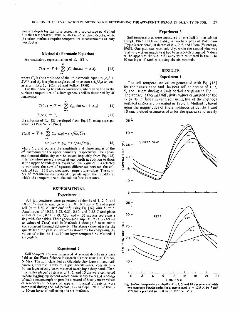
The soil temperature values generated with Eq. [16]for the quartz sand and the peat soil at depths of 1, 2,5, and 10 cm during a 24-h period are given in Fig. 1.The apparent thermal diffusivity values estimated for the1- to 10-cm layer in each soil using five of the methodsoutlined earlier are presented in Table 1. Method 1, basedupon the magnitudes of the amplitudes at depths 1 and10 cm, yielded estimates of a for the quartz sand nearly

35

30

QUARTZ SAND

ujK

% 20<EUJQ.

ui 15

10

35

30

I __ i i I _____ I

20

15 -

10 -

PEAT

9 12 15T I M E (hrs)

18 21 24

Fig. 1 — Soil temperature at depths of 1, 2, 5, and 10 cm generated withfive harmonic Fourier series for a quartz sand (as-') and a peat soil (a = 0.86 X 10~3 cm2 s-I

12.5 X 10"3 cm2

28 SOIL SCI. SOC. AM. J., VOL. 47, 1983

identical to the standard value; however, the estimate ofa for the peat soil was more than twice as large as thestandard. The phase equation of Method 2 yielded a val-ues which were 2.03 and 1.34 times as large as the stan-dard for the quartz sand and peat soil, respectively. Es-timates of a from these two methods (both based upona single sine term describing the surface soil temperature)failed to agree with each other. The common practice ofaveraging the values of a from both methods would haveproduced values that differed by 52 and 80% from thestandard values of a for the quartz sand and peat soils,respectively.

The Arctan Method (3) underestimated the standarda value for the quartz sand and overestimated a for thepeat soil. Estimates of a by the Logarithm Method (4)were slightly high for both soils. Temperatures at eachdepth for the arbitrary times of 0100, 0700, 1300, and1900 (1 and 10 cm) were used for Methods 3 and 4.Even for a day with clear skies and approximately sin-usoidal soil temperatures, the timing of the four pairs oftemperature measurements greatly affected the calculatedvalue of a. For the quartz sand Table 2 lists values of acalculated by Methods 3 and 4 for 12 different beginningtimes. The mean of a for the 12 different calculations isnearly identical to the standard value (12.58 X 10~3 cm2

s"1 for Method 3 and 12.53 X 10"3 cm2 s~l for Method4). However, a particular calculated value of a was asmuch as 8% (Method 4) to 15% (Method 3) differentfrom the standard value of a.

Table 1—Values of the apparent thermal diffusivity (10~'cm2 s"1)from experiment 1 for the 1- to 10-cm layer of quartz sand and

peat soil calculated using Methods 1 through 5.

No.

123456

Method

Title

AmplitudePhaseArctanLogarithmNumericalStandard

Quartz sand

Of

12.5725.4311.3013.1612.6012.50t

a/urSTD

1.012.030.901.051.011.00

Peat soil

a

1.951.151.880.900.890.86t

a/aSTD

2.271.342.191.051.031.00

f These values of the apparent thermal diffusivity ǤTD were used to gen-erate the soil temperatures from which values of a were calculated bythe five methods.

Table 2—Values of a for the quartz sand based upon Methods 3and 4 using different times at which temperatures are

observed(«STD = 12.5 x 10"'cm2 s~').

Beginning time

oioot0130J0200023003000330040004300500053006000630Mean

SD

Method 3

10-' em's'1

11.312.113.114.214.714.513.912.931.911.210.810.812.6

1.5

Method 4

10-' em's-'

13.112.712.111.711.511.611.812.312.813.313.513.4

12.50.8

The Numerical Method (5) based upon temperaturevalues measured every 0.5 h during the 24-h period, pro-duced estimates of a that were within 3% of the standardvalues. Even closer agreement is possible by reducing thechoice of Az and Af in Eq. [11]. Stability criteria for Eq.[11] are provided by Eq. [12], but there are no explicitcriteria available to ensure accuracy of the numericalscheme. The accuracy of Method 5 is obviously dependentupon the number of temperature observations used indescribing T(z,t). Values of a calculated from 4, 6, 8,12, and 24 values of T at each depth (1 and 10 cm) arepresented in Table 3. In a manner similar to that illus-trated in Table 2, for a given number of data points,several sets of calculations were made by selecting dif-ferent times at which the first value of T was taken.Calculated values of a were reasonably consistent wheneight data points per depth (temperature observationsevery 3 h) were used. Although improvement in calcu-lation of a was found with measurements every 2 h vs.every 3 h, little improvement in accuracy was found usingtemperature measurements at hourly or one-half-hourlyintervals vs. every 2 h.

Table 4 contains values of a calculated by Method 6for two-harmonic models using different numbers of tem-perature observations. Temperature observations recordedevery 3 h are required for an accurate determination ofa.

Experiment 2Observed temperature variations at depths of 1 and 10

cm below the surface of a bare soil over a 3-d period areshown in Fig. 2. The periodic nature of temperature var-iation can be seen at both depths, with greater diurnalvariations occurring at the shallower depth. The solidlines in Fig. 2 were obtained by fitting six harmonic Four-ier series to the data (Eq. [13]).

Estimates of a based upon Methods 1 through 6 usingthe soil temperature data presented in Fig. 2 are presentedin Table 5. Daily estimates of a are shown along with

Table 3—Values of 5 and its standard deviation (SD) for thequartz sand based upon Method 5 using different times at

which temperatures are observed (<XSTD =

12.5 x 10-' cm2 s-1).

No. data pointsperdeptht

468

1224

Sets

128642

10-' cm2 s-'

17.514.613.312.712.6

SD

10"'cm2s-'

4.44.30.50.1

<0.1

t Taken at equal time intervals.

Table 4—Values of a and its standard deviation (SD) for thequartz sand based upon Method 6 for 2 harmonics using

different times at which temperatures are observed(«STD = 12-5 x 10-3cm! s-'».

t Temperatures taken at 0100,0700,1300, and 1900 h.t Temperatures taken at 0130, 0730,1330. and 1930 h.

No. data pointsper depth!

68

1224

Sets

8642

«

10-3 cm1 s-

12.612.412.512.5

SD

10"'cm2s-'

1.8<0.2<0.2<0.2

t Taken at equal time intervals.

HORTON ET AL.: EVALUATION OF METHODS FOR DETERMINING THE APPARENT THERMAL DIFFUSIVITY OF SOIL 29

mean values of a for the 3-d period. Also estimates of afor the 3-d period were made. For the latter, values ofT averaged over the 3-d period were used in the 1-dequations of Methods 1 through 4. Observations of tem-perature for each depth (1 and 10 cm) were used in Eq.[11] (Method 5) and a was selected to minimize the sumof squared differences of calculated and measured tem-perature at the 5-cm depth. In Method 6, 72 (3 X 24per day) temperature observations at 1 cm were describedwith Eq. [14] whose coefficients were used to calculatea in Eq. [16]. The value of a was selected to minimizethe sum of squared differences of calculated and measuredtemperature at the 10-cm depth.

A wide range of a values exists (Table 5). As in ex-periment 1, estimates based upon a sinusoidal temperaturevariation at the surface (Methods 1 and 2) did not agree,and estimates via Method 2 were larger than via Method1. Although estimates of a from Methods 3 and 4 differed,their range was smaller than that for Methods 1 and 2.Methods 5 and 6 gave the most consistent estimates ofa with values of a ranging between 5.7 and 6.2 for Method5, and between 4.9 and 5.2 for Method 6.

Experiment 3Estimates of a for the 1- to 10-cm layer in the irrigated

and nonirrigated soils using Methods 1 through 6 arepresented in Table 6. The range in values of a was muchless for the dry soil than the wet soil. Values of a fromMethods 1 and 2 varied greatly for the irrigated site butwere relatively consistent for the nonirrigated site. Meth-ods 3 and 4 resulted in relatively large differences in theirestimates of a for both soils. Methods 5 and 6 differedslightly in estimations of a for both the wet and dry soils.

DISCUSSIONWhen partly cloudy conditions prevail, the occurrence

of two or more relative maxima may yield ambiguousvalues of a calculated from Methods 1 and 2. Figure 3depicts soil temperature at depths of 0, 1, 5, and 10 cmassociated with shading from cloud cover near mid-day.In this case two relative maximum temperatures wereobserved. With intermittent cloud cover several relativemaxima and minima per day may be realized. The in-

fluence of cloud cover on soil temperature variation atthe very shallow depths was large. For the 0-cm soil depth(Fig. 3a), the first relative maximum temperature at about1200 h was greater than the second relative maximumtemperature (at about 1500 h), while at the next twogreater depths, the second relative maximum was greaterthan the first. At the fourth depth (Fig. 3d), there wasonly one relative maximum value and its occurrence cor-responded with that of the second relative maxima at thethree shallower depths. Hence, on partially cloudy days,the ratio of noncorresponding amplitudes and their in-consistent occurrence yielding noncorresponding phaseangles result in erroneous estimates of a.

In experiment 1 calculations regarding the impact ofthe quantity of available data were made using Methods3 through 6. Similar calculations were made using thedata from experiments 2 and 3 (Table 7 and Table 8,respectively). In both cases the values of a calculated byMethods 3 and 4 differ substantially. Additionally, thestandard deviations of the calculated a's obtained withMethods 3 and 4 are much larger for the cloudy day(experiment 3, Table 8) than for the clear day (experiment2, Table 7). The relatively large standard deviations ob-tained with Methods 3 and 4 indicate that several cal-culations of a per day should be averaged in order tomake more suitable use of these methods. Calculationshave shown that a should be based on not less than threecalculations per day.

Although it is now established that Methods 3 and 4each require bihourly measures of temperature to computevalues of a consistent with those computed when morefrequent measures of temperature are available, the ac-curacy of a has not been evaluated. In experiment 1,Methods 3 and 4 produced about the same values of a(Table 2), but in experiments 2 and 3 large differencesin a were found (Tables 7 and 8). In experiment 1 thetemperatures represented a clear day, and a two-harmonicfunction described temperature variations very closely atboth the 1- and 10-cm depths. Because of this both Meth-ods 3 and 4 were consistent. However, in experiments 2

Table 5—Values of apparent thermal diffusivity (10~3 cm2 s"')from experiment 2 for the 1- to 10-cm depths calculated

from field data observed 12-14 Sept. 1980.

No.

123456

Method

Title

AmplitudePhaseArctanLogarithmNumericalHarmonic

12 Sept.

3.810.76.23.95.94.9

13 Sept.

4.46.96.23.95.75.1

(V

14 Sept.

4.110.75.73.56.25.2

3-d mean

4.19.56.03.85.95.1

12-14Sept.

4.1t9.2f6.0t3.7t5.85.1

t Values for Methods 1 through 4 are calculated from values of T(z,t) aver-aged over the 3-d period.

Table 6—Values of the apparent thermal diffusivity (10"' cm2 s"1)from experiment 3 for the 1- to 10-cm depth calculated from

field data observed 2 Sept. 1967.

24 36 46TIME (hrs)

Fig. 2—Hourly mean values of temperature measured at 1 and 10 cmin bare soil at Las Graces, N. Mex. from 12-14 Sept. 1980. The solidlines are fitted to the data with a 6-harmonic curve fit.

No.

123456

Method

Title

AmplitudePhaseArctanLogarithmNumericalHarmonic

Irrigated site

«

3.2910.74

7.324.835.173.94

Nonirrigated site

(V

1.271.723.721.591.441.75

30 SOIL SCI. SOC. AM. J., VOL. 47, 1983

56

48

532truo.5 24

• + 4- OBSERVED

F I T T E D56

48

32

a.5 24

42

- 30

24

5 18

• * - - * •+ OBSERVED

———— F I T T E D42

36

Z 30

IT

5 2 4ITUJ

•*• -f OBSERVED

FITTED

f • 29.08 C

9 12 ISTIME (hit)

18 24 9 12 15TIME (hrt)

IB 21

Fig. 3—Values of temperature measured at 0, 1, 5, and 10 cm in a nonirrigated bare soil and a Fourier series representation of the temperature ateach depth.

and 3 the field-measured temperatures were less well de-scribed by a two-harmonic function, especially the tem-perature variation at 1 cm. Because Methods 3 and 4 arebased on a two-harmonic function, the methods may beexpected to yield less consistent thermal diffusivity valuesnear the soil surface. Although the ease of calculationwarrants some merit, the differences in values of a ob-tained with these methods underline their limitations.

For clear days Methods 5 and 6 require at least eightvalues of temperature per depth (temperature measuredevery 3 h) in order to adequately calculate a. With in-creased numbers of observations little change in the valueof the standard deviation of a and of a was found. How-ever, for data representative of cloudy days more frequenttemperature observations were required in order to reducethe standard deviation and to obtain consistency in thecalculation of a. The numerical procedure of Method 5required, at most, hourly intervals (24 observations per

Table 7—Mean values of the apparent thermal diffusivity a(10 ' cm2 s~') and their standard deviations, s.

experiment 2,12 Sept. 1980. fNo. data

per depth

468

1224

Method 3

Sets

64321

ct

6.28na§nanana

s

0.94nananana

Method 4

«

3.95nananana

s

0.17nananana

Method 5

(K

7.285.705.635.865.90

s

3.011.280.310.20

Method 6}

(*

na}4.854.834.814.83

s

na0.660.150.04

t Based upon Methods 3 through 6 using different times at which tempera-tures are observed.

} Two harmonics only.§ Not applicable.

day), but was improved by going to one-half-h intervals.Method 6 did well with data acquired at 3-h intervalsbut improved with an interval of 2 h (Table 8).

In most cases the values of a calculated with Methods5 and 6 differed from each other. This result is not com-pletely unexpected in that temperature measurements atthree depths were required by Method 5 while measure-ments at only two depths were required by Method 6.Furthermore, the depths at which temperatures were fit-ted to obtain a differed for the two methods (5 cm forMethod 5 and 10 cm for Method 6). A test for accuracyof the calculated a's is to compare predicted with mea-sured soil temperatures. The depths fitted for selectionof a for experiment 3 data are shown in Fig. 4. Althoughdifferent values were found for a, the temperatures at 5and 10 cm were fitted very well using Methods 5 and 6,

Table 8—Mean values of the apparent thermal diffusivities «(10 ' cm2 s~') and their standard deviations, s, for the

irrigated plot from experiment 3.t

No. data

per depth

468122448

Method 3

Sets

1286421

(V

4.94na§nananana

s "

1.44nanananana

Method 4

(V

3.73nanananana

s

1.01nanananana

Method 5

<*

8.556.565.815.145.175.17

s

2.813.122.610.770.39

Method 6}

(V

na}4.053.993.963.973.97

s

na0.800.470.200.13

t Based upon Methods 3 through 6 using different times at which tempera-tures are observed. .

} Two harmonics only.§ Not applicable.

HORTON ET AL.: EVALUATION OF METHODS FOR DETERMINING THE APPARENT THERMAL DIFFUSIVITY OF SOIL 31

40 r- 40

35

30

UJaa

5 20ITui0.

g 15l-

1040

35

30

H 2 5UJac

METHOD 5

• • • OBSERVED IcmA » * OBSERVED 5cm———— PREDICTED 5cm

20IEUJ0.z 15 -

10

METHOD 6

OBSERVED IcmOBSERVED lOcmPREDICTED 10cm

18 21 243 6 9 12 15TIME (hrs)

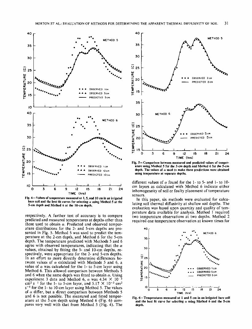
Fig. 4—Values of temperature measured at 1,5, and 10 cm in an irrigatedbare soil and the best fit curves for selecting a using Method 5 at the5-cm depth and Method 6 at the 10-cm depth.

respectively. A further test of accuracy is to comparepredicted and measured temperatures at depths other thanthose used to obtain a. Predicted and observed temper-ature distributions for the 2- and 5-cm depths are pre-sented in Fig. 5. Method 5 was used to predict the tem-perature at the 2-cm depth, and Method 6 for the 5-cmdepth. The temperature predicted with Methods 5 and 6agree with observed temperatures, indicating that the avalues, obtained by fitting the 5- and 10-cm depths, re-spectively, were appropriate for the 2- and 5-cm depths.In an effort to more directly determine differences be-tween values of a calculated with Methods 5 and 6, avalue of a was calculated for the 1- to 5-cm layer usingMethod 6. This allowed comparison between Methods 5and 6 when the same depth was fitted to obtain «. Usingexperiment 3 data and Method 6, a was 4.34 X 10~3

cm2 s~l for the 1- to 5-cm layer, and 5.17 X 10~3 cm2

s~' for the 1- to 10-cm layer using Method 5. The valuesof a differ, but a direct comparison between Methods 5and 6 is not possible. The measured and fitted temper-ature at the 5-cm depth using Method 6 (Fig. 6) com-pares very well with that from Method 5 (Fig. 4). The

35

30

H 25UJoc5 20ccUJ0.

ul 15

35

30

UJ(T3< 20ccUJa.S 1 5

METHOD 5

METHOD 6

OBSERVED 5cmPREDICTED 5cm

9 12 ISTIME (hrs)

18 21 24

Fig. 5—Comparison between measured and predicted values of temper-ature using Method 5 for the 2-cm depth and Method 6 for the 5-cmdepth. The values of a used to make these predictions were obtainedusing temperature at separate depths.

different values of a found for the 1- to 5- and 1- to 10-cm layers as calculated with Method 6 indicate eitherinhomogeneity of soil or faulty placement of temperaturesensors.

In this paper, six methods were evaluated for calcu-lating soil thermal diffusivity at shallow soil depths. Theevaluation was based upon quantity and quality of tem-perature data available for analysis. Method 1 requiredtwo temperature observations at two depths. Method 2required one temperature observation at known times for

40

35

30 -

-25

20

15

10

METHOD 6

OBSERVED 1 cmOBSERVED 5cmPREDICTED 5cm

9 12 15TIME (hrs)

IS 21 24

Fig. 6—Temperatures measured at 1 and 5 cm in an irrigated bare soiland the best fit curve for selecting or using Method 6 and the 5-cmdepth.

32 SOIL SCI. SOC. AM. J., VOL. 47, 1983

two depths. Both methods proved to be poor estimatorsof a near the soil surface. Methods 3 and 4 required fourmeasures of temperature equally spaced in time at twodepths. Both methods were erratic, but improved if tem-peratures were measured bihourly and all estimates of aaveraged. Method 5 was a reliable estimator of a if suf-ficient temperature data were available. For clear days,eight observations at each of three depths were required.On cloudy days, hourly measures of temperature at threedepths were required. Finally, Method 6 was found to bevery consistent with the least amount of required data.For both clear and cloudy days, only 8 to 12 temperatureobservations at two depths were required to obtain con-sistent estimates of the apparent thermal diffusivity. Be-cause Method 6 is reliable and requires fewer tempera-ture data than Method 5, it is recommended as the mostadvantageous of the six methods for determining the ap-parent thermal diffusivity near the soil surface.

Future work should evaluate the impact of the qualityand quantity of temperature data on the calculation ofthe depth dependence of the apparent thermal diffusivity.