evaluation of japan’s macro-fiscal policy and its challenges

1

Evaluation of Japan’s Macro-Fiscal Policy and its Challenges＊

FUKUDA Shin-ichiProfessor, Graduate School of Economics, University of Tokyo

SOMA NaotoAssociate Professor, Faculty of International Social Sciences, Division of International Social Sciences, Yokohama Nation-al University

AbstractThis study aims to examine the effectiveness of macro-fiscal policy conceptually to de-

rive empirical implications for the Japanese economy. Since the mid-1990s, Japan has re-mained stuck in a liquidity trap, where interest rates fall to or are below zero. However, not only has the cumulative fiscal deficit increased to an unprecedented level, but many structur-al problems have also emerged. Under these circumstances, previous empirical findings are inconclusive regarding whether fiscal policy has worked effectively in the Japanese econo-my. This study reexamined the findings of previous studies based on data for the period since 1980 and considered the challenges for such analyses. When a reduced-form equation or a VAR model was estimated, we found that the effects of fiscal expenditure, which had declined over the medium- to long-term period, may have increased since the fourth quarter of 2010. This finding suggests that the steadily falling effects of the fiscal expenditure may have recovered under ultra-low interest rates. Using the ESP Forecast Survey, representing the forecast data prepared by private-sector economists, it was confirmed that these econo-mists assumed the presence of a significant correlation between fiscal expenditure and GDP under ultra-low interest rates. However, the results must be carefully interpreted with re-spect to the limitations of the estimation method, including outliers, the reference year for GDP used in the analysis, and the robustness of the sample period. As the conclusion of this paper is based on a short sample period whose estimation efficiency is not necessarily high, it is unclear whether the effects of fiscal expenditure will continue to improve. In addition, the results obtained through a reduced-form equation or a VAR model indicate the presence of a Granger causality but not the presence of a true causal relationship. In the field of mac-roeconomics, the effectiveness of fiscal policy has been discussed for many years. This study’s findings should be verified in the future to check its robustness.

Keywords: fiscal policy, structural changes, ultra-low interest rates, ESP ForecastJEL Classification: E62, H30, E3

＊ This article is based on a study first published in the Financial Review No. 144, pp. 156-180, Fukuda and Soma (2021), “Evaluation of Macro-Fiscal Policy and Challenges in Japan” written in Japanese. We would like to thank participants of PRI review meeting for their helpful comments.

Policy Research Institute, Ministry of Finance, Japan, Public Policy Review, Vol.17, No.2, November 2021

I. Introduction

In macroeconomics, analyzing the effectiveness of fiscal policy in raising national in-come is an old and new question that has been debated for many years. This study aims to provide an extensive overview of macro-fiscal policy, focusing on the empirical results of the Japanese economy. Considering the effectiveness of macro-fiscal policy, the Japanese economy has exhibited three major characteristics in recent years.

First, since the mid-1990s, the economy has been under a “liquidity trap,” in which in-terest rates are zero or negative. If interest rates rise because of increased fiscal spending, a “crowding out” of private investment will occur, leading to a relatively small effect of fiscal policy on national income. However, as interest rates do not fall under the liquidity trap, the effects of fiscal policy are larger than those of crowding out. In addition, as Blanchard (2019) indicates, under zero or negative interest rates, the costs of expanding government debt are small because of the minor negative effects of fiscal deficit.

Second, the accumulation of fiscal deficit has reached a globally unprecedented level, which other major countries have never experienced. Therefore, although interest rates are historically low, the burden on future generations has become extremely heavy. To the ex-tent that the government is “Ricardian” behavior, being responsible for repaying the deficit, the accumulation of fiscal deficit may cause a “non-Keynesian effect” on private consump-tion when people have serious concerns about future burdens. In this case, a decline in the propensity to consume offsets the effects of fiscal policy on national income from the per-spective of long-term sustainability. Thus, if the non-Keynesian effect is large, the expansion of fiscal spending may even be counterproductive.

Third, after the bursting of the bubble, various structural problems have emerged, lead-ing to long-term stagnation. For example, the bubble burst in the early 1990s led to the emergence of “zombie companies,” primarily in the non-manufacturing sector. “Zombie companies” refer to those companies that would otherwise have to exit the market. In the late 1990s and early 2000s, persistent financial support for zombie companies could have further delayed economic recovery1. In addition, social security-related expenditures have increased owing to the declining birthrate and aging population. Thus, income transfer has claimed a substantial portion of government expenditure, which has been less effective in increasing national income in Keynesian economics.

Traditional macroeconomic frameworks, such as IS-LM analysis, tended to emphasize the first characteristic and conclude that fiscal policy is extremely effective under the “li-quidity trap.” However, if the second and third characteristics are important, the effective-ness of fiscal policy will be relatively low. When considering the effectiveness of Japan’s fiscal policy, it is important to reconsider the characteristic that is more important than the others in Japan’s context.

1 For the impact of zombie companies on the Japanese economy, see Hoshi (2006), Caballero, Hoshi and Kashyap (2008), and Fukuda and Nakamura (2011).

2 FUKUDA Shin-ichi, SOMA Naoto / Public Policy Review

3

In previous studies, Miyamoto, Nguyen, and Sergeyev (2018) showed that the effective-ness of Japan’s fiscal policy greatly increased under a “liquidity trap,” even though Kato, Miyamoto, Nguyen, and Sergeyev (2018) pointed out that tax cuts were less effective. Bay-oumi (2001), Kuttner and Posen (2001, 2002), and Morita (2015), using a multivariate au-toregressive (VAR) model, and Kameda, Nambaz, and Tsuruga (2021), using panel data by prefecture, found that fiscal policy continued to be effective after the 1990s in Japan. Con-trarily, focusing on the structural problem of a rapidly aging society with a declining birth-rate, Yoshino and Miyamoto (2017) showed calibration results in which the effectiveness of Japan’s fiscal policy declined. Werner (2004) and Auerbach and Gorodnichenko (2017) also indicated that the multiplier effect of fiscal policy, which was effective from a medium- to long-term perspective, has been on a declining trend in recent years. Umeda et al. (2018) found that many Japanese economists believed that the multiplier effect has declined.

Thus far, the empirical analysis has largely been controversial over whether fiscal policy has been effective in the Japanese economy in recent years. However, it is impossible to simply compare the results of the abovementioned studies because they used different ana-lytical frameworks as well as different sample periods. Therefore, in this study, we update the data of these previous studies and review the robustness of the results through the esti-mation of reduced-form equations and VAR models. We also examine private economists’ views on the impact of fiscal spending by using the forecast survey data “ESP Forecast.”

II. “Government Expenditures” used in the analysis

II-1. Concept of “government expenditures”

Before starting the empirical analysis, this section first summarizes the concept of “gov-ernment expenditures” used in the following analysis. The “government expenditures” in-clude “government consumption” and “public investment” based on the “National Accounts (GDP statistics)” (benchmark year 2011 [2008 SNA]). They are substantially different from the total expenditures by the central and local governments in two respects.

First, they are expenditures by the “general government,” composed not only of central and local governments’ expenditure but also of social security funds. The central govern-ment’s expenditures include those of the general account and the special account and inde-pendent administrative agencies. Local governments’ expenditures include those of the local government’s general account as well as local public businesses and local independent ad-ministrative agencies. Social security funds include the central government’s special account for public pension and employment insurance, the local government’s account for medical services and nursing care services, a part of the civil servant mutual aid association account, and the Government Pension Investment Fund.

Figure 1 shows that government consumption from FY2005 to FY2018 can be divided into those of central and local governments and social security funds. The central govern-ment’s share was small, from 17% in 2005 to 14% in 2018. Contrarily, the share of local


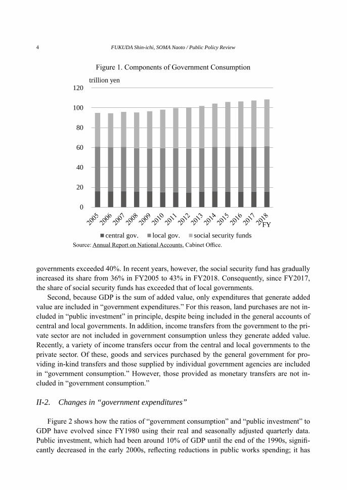
governments exceeded 40%. In recent years, however, the social security fund has gradually increased its share from 36% in FY2005 to 43% in FY2018. Consequently, since FY2017, the share of social security funds has exceeded that of local governments.

Second, because GDP is the sum of added value, only expenditures that generate added value are included in “government expenditures.” For this reason, land purchases are not in-cluded in “public investment” in principle, despite being included in the general accounts of central and local governments. In addition, income transfers from the government to the pri-vate sector are not included in government consumption unless they generate added value. Recently, a variety of income transfers occur from the central and local governments to the private sector. Of these, goods and services purchased by the general government for pro-viding in-kind transfers and those supplied by individual government agencies are included in “government consumption.” However, those provided as monetary transfers are not in-cluded in “government consumption.”

II-2. Changes in “government expenditures”

Figure 2 shows how the ratios of “government consumption” and “public investment” to GDP have evolved since FY1980 using their real and seasonally adjusted quarterly data. Public investment, which had been around 10% of GDP until the end of the 1990s, signifi-cantly decreased in the early 2000s, reflecting reductions in public works spending; it has

Figure 1. Components of Government Consumption

Source: Annual Report on National Accounts, Cabinet Office.

0

20

40

60

80

100

120trillion yen

FYcentral gov. local gov. social security funds


5

been around 5% of GDP since FY2007. However, government consumption has been steadi-ly increasing since the 1990s, from approximately 15% of the GDP in the early 1990s to around 20% since 20092.

Figure 3 depicts, in nominal terms, the changes in the breakdown of “government con-sumption” by its function since FY2005. It shows that expenditures for general administra-tion have been greatly reduced in recent years, from nearly 11 trillion yen in FY2005 to less than nine trillion yen in FY2012 and thereafter. However, there has been a huge increase in “health” expenditures such as medical expenses and “social assistance” expenditures such as welfare benefits. “Health” expenditures were about 30 trillion yen in FY2005, but they exceeded 40 trillion yen in FY2018. “Social assistance” expenditures were about 9.4 trillion yen in FY2005, but they exceeded 14 trillion yen in FY2017. Thus, the increase in social se-curity-related expenditures was a major factor in the recent increases in “government con-sumption.”

Figure 4 shows how the short-term fluctuations in “government consumption” and “pub-lic investment” have changed since FY1980 using the quarterly (annualized) changes of their real and seasonally adjusted data. From the figure, we can see that there were consider-able short-term fluctuations in the 1980s for “government consumption” and in the 1980s and 1990s for “public investment.” At that time, “public investment” typically exhibited large short-term fluctuations. However, in the 2000s, short-term fluctuations significantly decreased in both “government consumption” and “public investment.” After the collapse of

Figure 2. The Ratios of Government Consumption and Public Investment to GDP


0

5

10

15

20

2519

80Q

119

81Q

419

83Q

319

85Q

219

87Q

119

88Q

419

90Q

319

92Q

219

94Q

119

95Q

419

97Q

319

99Q

220

01Q

120

02Q

420

04Q

320

06Q

220

08Q

120

09Q

420

11Q

320

13Q

220

15Q

120

16Q

420

18Q

320

20Q

2

%

government consumption pubulic investment

2 Due to the revision of SNA, it is not possible to make a strict comparison between the data after FY1994 (benchmark year 2011) and that before FY1994 (benchmark year 2005). However, the above results are basically valid even after considering the discontinuity.


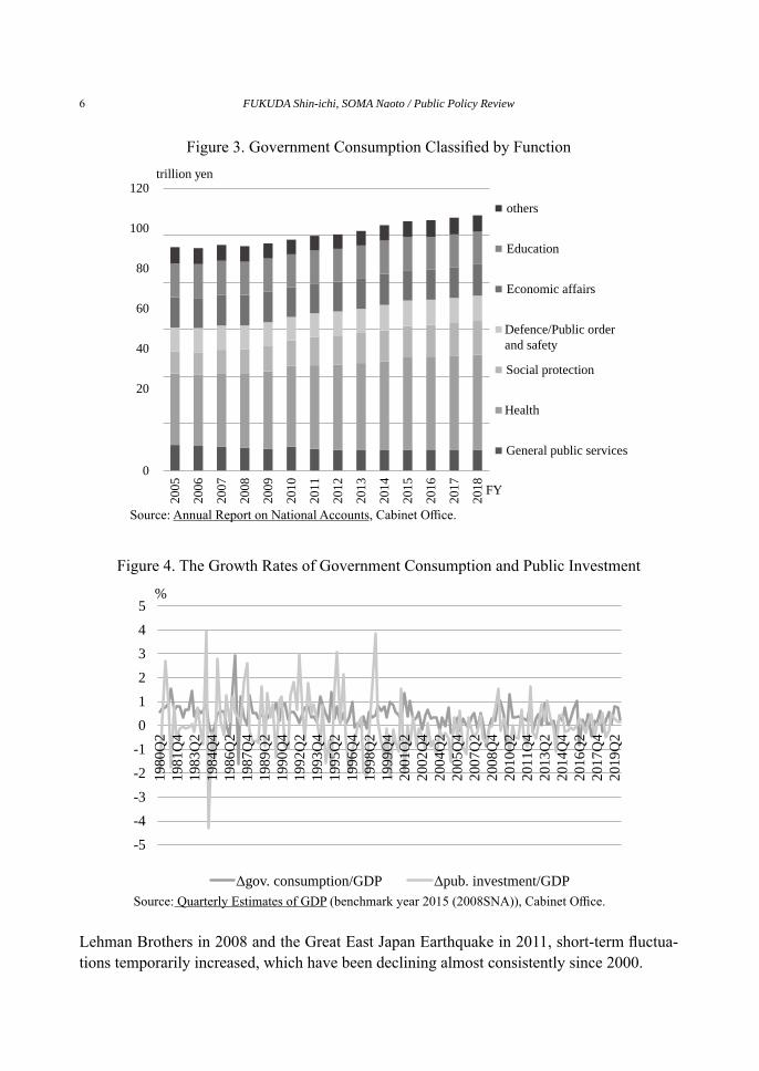
Lehman Brothers in 2008 and the Great East Japan Earthquake in 2011, short-term fluctua-tions temporarily increased, which have been declining almost consistently since 2000.

0

20

40

60

80

100

12020

05

2006

2007

2008

2009

2010

2011

2012

2013

2014

2015

2016

2017

2018

trillion yen

FY

General public services

Health

Social protection

Defence/Public order and safety

Economic affairs

Education

others

Figure 3. Government Consumption Classified by Function


-5-4-3-2-1012345

1980

Q2

1981

Q4

1983

Q2

1984

Q4

1986

Q2

1987

Q4

1989

Q2

1990

Q4

1992

Q2

1993

Q4

1995

Q2

1996

Q4

1998

Q2

1999

Q4

2001

Q2

2002

Q4

2004

Q2

2005

Q4

2007

Q2

2008

Q4

2010

Q2

2011

Q4

2013

Q2

2014

Q4

2016

Q2

2017

Q4

2019

Q2

%

Δgov. consumption/GDP Δpub. investment/GDP

Figure 4. The Growth Rates of Government Consumption and Public Investment

Source: Quarterly Estimates of GDP (benchmark year 2015 (2008SNA)), Cabinet Office.


7

III. Alternative Perspectives in Previous Studies

In previous studies, two types of analyses were conducted to examine the effectiveness of Japan’s fiscal policy. The first type is an analysis of structural changes in the Japanese economy from medium- to long-term perspectives. They indicated that the effects of fiscal policy, which had been effective for many years, may have been decreasing in recent years. Many of these studies have evaluated how the effects of fiscal policy have changed over several decades and concluded that the effects in recent years have decreased in contrast with those in the high growth period of the 1950s and 1960s and the stable growth period of the 1970s and 1980s. The second type is an analysis of changes in the effectiveness of fiscal policy under the recent ultra-low interest rate environment. They argued that the effects of fiscal policy have been increasing in the ultra-low interest rate environment in recent years. Many of these studies suggested that the effects of fiscal policy may have been greater in periods when interest rates are zero or negative than in previous periods.

However, these types of analyses face challenges owing to limited data availability in Japan. The first type faces a challenge because there are no consistent time-series data of “National Accounts (GDP Statistics)” from the 1950s to the 2000s. We can obtain consistent data from the first quarter of 1955 to that of 1999 by the benchmark year 1990 (1968 SNA). We can also obtain consistent data from the first quarter of 1980 to the second quarter of 2020 (including simple retrospective data) by the benchmark year 2011 (2008 SNA). In ad-dition, although the period is somewhat shorter, data are available for the period from the first quarter of 1980 to the second quarter of 2005 by the benchmark year 1995 (1993 SNA), the first quarter of 1980 to the third quarter of 2011 by the benchmark year 2000 (1993 SNA), the first quarter of 1980 to the third quarter of 2016 by the benchmark year 2005 (1993 SNA) (including simple retrospective data), and the first quarter of 1994 to the latest by the benchmark year 2015 (2008 SNA). However, the data from the benchmark year 1990 (1968 SNA) has not included periods with ultra-low interest rates in recent years. In con-trast, the other data do not include periods of high economic growth in the 1950s and 1960s and the stable growth period of the 1970s. Therefore, when analyzing policy effects from a medium- to long-term perspective, many previous studies conducted comparative analyses by connecting GDP statistics that were constructed using different methods and benchmark years.

However, it is not appropriate to examine the medium- to long-term effects of fiscal pol-icy using a connected series of GDP statistics. Table 1 shows how the data series constructed by one benchmark year were correlated with those constructed by another benchmark year, using seasonally adjusted quarterly data of real GDP, government expenditures (= govern-ment consumption + public investment), and public investment. When calculating the cor-relation coefficients, we used three benchmark years: 1990 (1968 SNA), 2000 (1993 SNA), and 2011 (2008 SNA). Although they were constructed using different methods and bench-mark years, they commonly provide time-series data from the second quarter of 1980 to the first quarter of 1999. The correlation is that of the growth rates (logged differences) of each


variable. The table shows that the 1993 SNA and 2008 SNA were highly correlated. The correlation was greater than 0.9. However, the 1968 SNA was not strongly correlated with the 1993 SNA and the 2008 SNA. The correlation ranged from 0.565 to 0.695.

Table 2 shows how the correlation coefficient between real GDP and government expen-ditures or public investment differs depending on the three benchmark years. The correlation coefficient is calculated using the growth rates (logged differences) of seasonally adjusted quarterly series from the second quarter of 1980 to the first quarter of 1999. The correlation coefficient between real GDP and government expenditures was the highest at the 2008 SNA at 0.255, while it was the lowest at the 1993 SNA at 0.140. The correlation coefficient between real GDP and public investment was the highest at the 1968 SNA at 0.214, while it was the lowest at the 1993 SNA at 0.088. These results suggest that connecting GDP statis-tics constructed using different methods and benchmark years may cause serious problems.

On the contrary, the second type faces a challenge because the sample period in the ul-

Table 1. Correlation Coefficient of GDP Statistics by Different Methods and Benchmark Years(1) The growth rate of real GDP

1968SNA 1993SNA 2008SNA

1968SNA 1.000

1993SNA 0.575 1.000

2008SNA 0.563 0.938 1.000

1968SNA 1993SNA 2008SNA

1968SNA 1.000

1993SNA 0.695 1.000

2008SNA 0.613 0.933 1.000

(2) The growth rate of real government expenditures

1968SNA 1993SNA 2008SNA

1968SNA 1.000

1993SNA 0.641 1.000

2008SNA 0.582 0.920 1.000

(3) The growth rate of real public investment

Table 2. Correlation Coefficient between GDP and Government Expenditures

Note. The correlation coefficient is calculated using their growth rates.

1968SNA 1993SNA 2008SNA

gov. expenditure 0.175 0.140 0.255

public investment 0.214 0.088 0.193


9

tra-low interest rate environment is small. The challenge occurs even if GDP statistics are constructed by the consistent method and benchmark year. In Japan, short-term interest rates have remained extremely low since the mid-1990s, with overnight call rates falling substan-tially throughout the 1990s: the official discount rate fell to 0.5% in 1995, and the zero-in-terest rate policy was launched in February 1999. However, long-term interest rates, such as the yield of 10-year government bonds, remained positive even under the zero-interest rate policy. It was not until October 2010, when the Bank of Japan started comprehensive mone-tary easing, that long-term interest rates began showing a clear downward trend. When ex-ploring the effects of fiscal policy, it is important to observe the stability of long-term inter-est rates. The sample size of the data is too small to test a structural change in the effects of fiscal policy between and prior to the periods under ultra-low long-term interest rates. Anal-ysis in a small sample period presents challenges in terms of the efficiency of estimation, and various considerations are required to interpret the results. The following sections of this paper will review the second type of analysis, recognizing this limitation.

IV. The Estimations of Reduced-form Equations

IV-1. Analytical framework

The following analysis examines whether there are structural changes in the effects of fiscal spending. The data used for the analysis are the national accounts (GDP statistics) of the benchmark year 2011 (2008 SNA)3. We use seasonally adjusted data from the first quar-ter of 1980 to the fourth quarter of 2019, even though simple retroactivity was applied from 1982 to 1993. As noted in the previous section, there are many challenges in analyzing structural changes using relatively short sample periods. However, given the limited avail-ability of data, we need to analyze structural changes using a relatively short sample period.

In the analysis, we first estimate the reduced-form equation and examine the structural changes in the impact of fiscal spending on the GDP. The estimation of the reduced-form equation has a limitation in that its economic structures are in a black box. In addition, the estimated “effect” is the “Granger causality,” which does not necessarily imply the true causal relation. However, the estimation of the reduced-form equation is the simplest meth-od to grasp the effect of exogenous variables, and it has been extensively used in previous research. We estimated the following equation, including lagged endogenous variables, us-ing seasonally adjusted quarterly data:

ΔYt = constant+∑2i=0 ai ΔGt – i +∑

2i=0 bi ΔYt – i +∑

1i=0 ci Xt – i, (1)

Here, ΔYt is the growth rate (logged difference) of real GDP, ΔGt is the increase (difference) in real government expenditures/real GDP in the previous period, and Xt is the control vari-able. For the control variable, we use the growth rate (logged difference) of real exports as 3 The analysis did not include the data for 2020 to exclude the enormous impacts of COVID-19 on the GDP.


the baseline estimate.The estimation is performed by the least-squares method and instrumental variable

method. We use the instrumental variable method because when the explanatory variable ΔG is determined endogenously, a simultaneous bias may occur. As Fukuda and Yamada (2011) pointed out, since the 1990s, the government has formulated economic measures and increased fiscal spending when a recession is expected. In such a case, the explanatory vari-able ΔG has a negative correlation with the error term in Equation (1). Thus, there is a possi-bility of “simultaneity bias,” in which the estimated value of the coefficient is smaller than the true value. In the following analysis, the constant term and the rate of increase in real exports were used as exogenous variables, and the lag values of all explanatory variables from period one to period three were used as instrumental variables. In addition, lagged val-ues of the following variables were added to the instrumental variables: the growth rate of real private consumption, the growth rate of real private non-residential investment, the rate of change in GDP deflator, ΔG, and the growth rate of the stock price index (Nikkei 225 at the end of the quarter).

IV-2. Timing of structural breaks

In examining structural changes during the sample period, it is important to determine when structural changes have occurred. Most previous studies divided the sample period by exogenous institutional changes, such as policy changes by the Bank of Japan, and explored whether there were any significant changes in the effectiveness of fiscal policy before and after the fixed structural changes. In contrast, this study uses the Quandt–Andrews Structur-al Break Test (Andrews 1993), typically used when the timing of structural changes is un-known, to determine when structural changes have occurred.

For the analysis, we first estimated Equation (1) for the sample period from the fourth quarter of 1980 to the fourth quarter of 2019 and then applied the Quandt–Andrews test to identify when structural changes have occurred in the estimated result. Table 3-1 summariz-es the results of the structural break tests. It showed that both the likelihood ratio test (LR) and the Wald test (Wald) had a significant structural change in the third quarter of 1991. The third quarter of 1991 coincided with the period when the bubble economy collapsed and po-tential growth rates fell4.

However, the sample period after the third quarter of 1991 includes both a period in which interest rates are significantly positive and a period in which interest rates have fallen to zero. We thus estimated Equation (1) again for the sample period from the third quarter of 1991 to the fourth quarter of 2019 and applied the Quandt–Andrews test to the estimation result. Table 3-2 summarizes the results of the structural break test. It showed that both the LR and Wald had structural changes at a 10% significance level in the fourth quarter of

4 February 1991 was the “peak” of the economy, according to the Committee for Business Cycle Indicators in the Cabinet Of-fice.


11

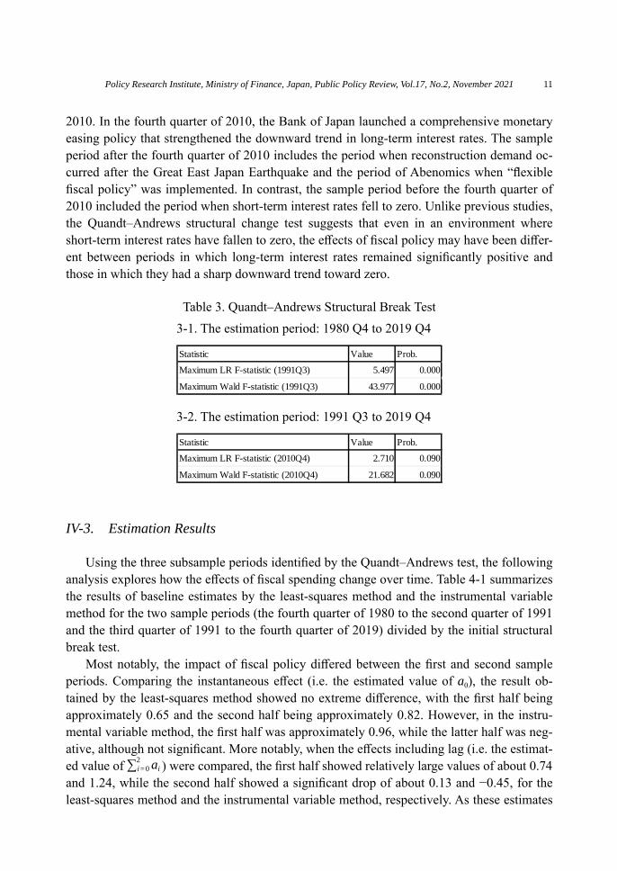
2010. In the fourth quarter of 2010, the Bank of Japan launched a comprehensive monetary easing policy that strengthened the downward trend in long-term interest rates. The sample period after the fourth quarter of 2010 includes the period when reconstruction demand oc-curred after the Great East Japan Earthquake and the period of Abenomics when “flexible fiscal policy” was implemented. In contrast, the sample period before the fourth quarter of 2010 included the period when short-term interest rates fell to zero. Unlike previous studies, the Quandt–Andrews structural change test suggests that even in an environment where short-term interest rates have fallen to zero, the effects of fiscal policy may have been differ-ent between periods in which long-term interest rates remained significantly positive and those in which they had a sharp downward trend toward zero.

IV-3. Estimation Results

Using the three subsample periods identified by the Quandt–Andrews test, the following analysis explores how the effects of fiscal spending change over time. Table 4-1 summarizes the results of baseline estimates by the least-squares method and the instrumental variable method for the two sample periods (the fourth quarter of 1980 to the second quarter of 1991 and the third quarter of 1991 to the fourth quarter of 2019) divided by the initial structural break test.

Most notably, the impact of fiscal policy differed between the first and second sample periods. Comparing the instantaneous effect (i.e. the estimated value of a0), the result ob-tained by the least-squares method showed no extreme difference, with the first half being approximately 0.65 and the second half being approximately 0.82. However, in the instru-mental variable method, the first half was approximately 0.96, while the latter half was neg-ative, although not significant. More notably, when the effects including lag (i.e. the estimat-ed value of ∑2

i=0 ai ) were compared, the first half showed relatively large values of about 0.74 and 1.24, while the second half showed a significant drop of about 0.13 and −0.45, for the least-squares method and the instrumental variable method, respectively. As these estimates

Table 3. Quandt–Andrews Structural Break Test3-1. The estimation period: 1980 Q4 to 2019 Q4

Statistic Value Prob.

Maximum LR F-statistic (1991Q3) 5.497 0.000

Maximum Wald F-statistic (1991Q3) 43.977 0.000

3-2. The estimation period: 1991 Q3 to 2019 Q4

Statistic Value Prob.

Maximum LR F-statistic (2010Q4) 2.710 0.090

Maximum Wald F-statistic (2010Q4) 21.682 0.090


are not highly significant, it is difficult to draw definitive conclusions from them. However, even from 1980 onward, the results show that the influence of fiscal policy has been declin-ing in recent years as a medium-term trend.

However, Table 4-2 summarizes the results of baseline estimation by the least-squares method and the instrumental variable method for the two sample periods (the second quarter of 1991 to the third quarter of 2010 and the fourth quarter of 2010 to the fourth quarter of 2019) divided by the second structural break test.

It is worth noting that a large value was observed only in the latter sample period in both the instantaneous effect and the total effect, including lags. The instantaneous effect shows that the first half had a negligible impact of about 0.54 and −0.38, while the second half had a large impact of about 2.39 and 2.34, respectively, for the least-squares method and the in-strumental variable method. By contrast, the total effect, including lags, shows that the first half had almost no effect with about 0.02 and −0.41, while the second half showed a signifi-cant effect with about 2.62 and 2.56, respectively, for the least-squares method and the in-strumental variable method. Both estimates indicate that the effects of fiscal policy has in-creased significantly since the fourth quarter of 2010.

Since the estimation of the reduced-form equation only shows the “Granger causality” rather than the true causality, we need more careful interpretations to conclude that “the pol-icy effect greatly increased.” The first half, however, includes the period when zombie com-panies became apparent and the period when spending cuts were implemented under fiscal reforms of the Koizumi administration. The Koizumi administration did not apply any fiscal stimulus. Contrarily, the second half coincides with the period in which long-term interest rates show a downward trend toward zero. Since the fourth quarter of 2010, the Bank of Ja-pan strengthened its unconventional monetary policy. Therefore, the above results are con-sistent with the view that the effects of fiscal policy have increased due to the “liquidity trap,” and the cost of expanding government debt is small under ultra-low interest rates.

However, it is worth noting that the short-term interest rates were virtually zero in most samples for the first half. No effect of fiscal spending was observed during that period, which is inconsistent with the argument that an ultra-low short-term interest rate policy en-hances fiscal policy effectiveness. Considering that long-term interest rates did not fall dis-continuously from the fourth quarter of 2010, the effects of fiscal spending may differ sig-nificantly, even under the same liquidity trap.

V. Estimations by VAR

In the previous section, we estimated the reduced-form equation to determine the struc-tural changes since the 1980s and examined how the impact of fiscal policy changed in Ja-pan. In this section, we use a vector autoregressive (VAR) model to examine the effects of fiscal policy on GDP over the same sample period. As with the reduced-form equation, the economic structures behind VAR are in a black box, and the “effects” showed by VAR are the “Granger causality,” which does not necessarily indicate the true causal relationship.


13

Whereas the reduced-form equation examines the unidirectional “impact” of government spending on GDP, the VAR examines the overall “impact” of government spending on GDP through various macro variables. As in the previous section, VAR models were estimated using seasonally adjusted quarterly data for each subsample period identified in the structur-

Notes 1) In the case of the instrumental variable method, the entire period starts from 1981Q1. 2) *** =significant at the 1% level, ** = significant at the 5% level, and * = significant at the 10% level. 3) ΣΔG(i) shows the total effect including lags.

Table 4. The Effects of Fiscal Spending on GDP4-1. The entire period

coeff. t value coeff. t value coeff. t value coeff. t value

C 0.014 4.350 *** 0.013 3.695 *** -0.001 -0.896 0.001 1.043

∆G 0.645 1.810 * 0.961 1.719 * 0.818 2.549 ** -0.306 -0.561

∆G(-1) 0.171 0.448 0.251 0.616 -0.224 -0.664 0.241 0.835

∆G(-2) -0.032 -0.087 0.026 0.067 -0.464 -1.470 -0.387 -1.553

∆Y(-1) -0.267 -1.617 -0.292 -1.705 * 0.017 0.126 -0.053 -0.485

∆Y(-2) -0.199 -1.207 -0.163 -0.918 0.063 0.649 0.099 1.287

∆EX 0.036 0.616 0.022 0.321 0.191 9.418 *** 0.164 10.229 ***

∆EX(-1) 0.036 0.628 0.047 0.776 -0.010 -0.320 -0.020 -0.817

Adj. R2 0.019 -0.037 0.449 0.454

DW stat 1.946 1.936 1.778 1.836

coeff. F-statistic coeff. F-statistic coeff. F-statistic coeff. F-statistic

Σ∆G(i) 0.784 1.045 1.238 1.609 0.130 0.080 -0.452 0.781348

The first subsample: 1980Q4 - 1991Q2

Ordinary least squares Instrumental variable

The second subsample: 1991Q3 - 2019Q4


4-2. The second subsample period


C -0.001 -0.952 0.001 0.629 0.000 -0.125 0.000 -0.092

∆G 0.540 1.976 * -0.377 -0.767 2.391 3.369 *** 2.343 2.807 ***

∆G(-1) -0.048 -0.168 0.372 1.284 -0.632 -0.860 -0.633 -0.861

∆G(-2) -0.469 -1.741 * -0.406 -1.588 0.865 1.164 0.848 1.118

∆Y(-1) -0.110 -0.814 -0.119 -0.930 0.230 1.263 0.229 1.257

∆Y(-2) 0.196 2.148 ** 0.187 2.160 ** -0.403 -2.636 ** -0.400 -2.554 **

∆EX 0.198 10.956 *** 0.166 9.693 *** 0.156 3.893 *** 0.156 3.882 ***

∆EX(-1) 0.006 0.208 -0.008 -0.289 -0.064 -1.253 -0.064 -1.255

Adj. R2 0.630 0.541 0.468 0.468

DW stat 1.965 1.902 1.704 1.705


Σ∆G(i) 0.023 0.004 -0.410 0.800 2.623 3.388 * 2.559 2.737

The second subsample I : 1991Q3 - 2010Q3 The second subsample II :2010Q4 - 2019Q4

Ordinary least squares Instrumental variable Ordinary least squares Instrumental variable


al break test.In the VAR model, ΔYt (≡ logged difference of real GDP), ΔGt (≡ increase in real gov-

ernment expenditures/real GDP in the previous period), and ΔPt (≡ logged difference of GDP deflator) were used as endogenous variables, and ΔEXt (≡ logged difference of real ex-ports) was used as the exogenous variable. Specifically, we estimate the following sec-ond-order VAR model5:

Xt = A1Xt− 1 + A2Xt− 2 + BZt, (4)

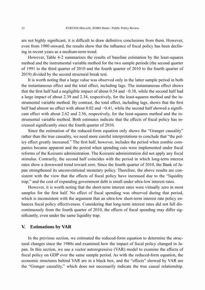
Here, Xt ≡ {ΔGt, ΔYt, ΔPt}, and Zt ≡ {the constant term, ΔEXt}.Figure 5-1 shows the cumulative impulse response functions of ΔYt to ΔGt when the en-

tire sample period was divided into the two sub-samples at the third quarter of 1991. The es-timated cumulative impulse response function showed no persistent impact of government spending on GDP in either period. In the first half (i.e. from the fourth quarter of 1980 to the second quarter of 1991), the value of the cumulative impulse response function was stable at 0.002 but was not statistically significant except in the first quarter. In the latter half of the period (i.e. from the third quarter of 1991 to the fourth quarter of 2019), the cumulative im-pulse response function showed a statistically significant value of 0.002 in the first two quarters but declined after the third quarter and became insignificant thereafter.

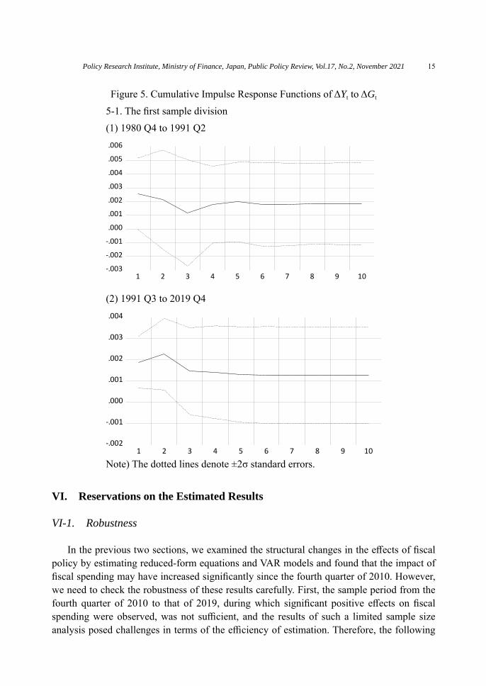
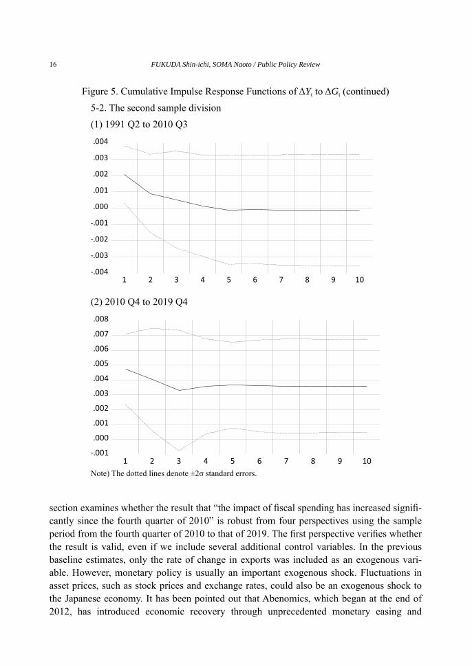
However, if the latter half of the sample is further divided in the fourth quarter of 2010, the result of the cumulative impulse response function changed significantly. Figure 5-2 shows the cumulative impulse response function of ΔYt to ΔGt when we split the latter half in the fourth quarter of 2010. In the first half (i.e. from the second quarter of 1991 to the third quarter of 2010), the cumulative impulse response function had a statistically signifi-cant value of 0.002 in the first quarter but dropped to almost zero after the second quarter. Conversely, in the latter half (i.e. from the fourth quarter of 2010 to the fourth quarter of 2019), not only was the cumulative impulse response function close to 0.05, which was sta-tistically significant in the first quarter, but it was also statistically significant after the sec-ond quarter, except in the third quarter. This result is consistent with the view that the impact of fiscal policy on GDP increased significantly since the third quarter of 2010.

However, even in the estimation from the third quarter of 2010 onward, the cumulative impulse response function had the largest value in the first quarter. This implies that even if there were significant policy effects, there was little ripple effect over time. Previous studies estimating VAR have shown that during the high growth period of the 1950s and 1960s and the stable growth period of the 1970s and 1980s, the cumulative impulse response function increased with time, producing various ripple effects. Such spillover effects may not be ob-served in the recent fiscal policy.

5 The identification was performed by Cholesky decomposition, where the order of exogeneity was ΔGt, ΔYt, and ΔPt.


15

VI. Reservations on the Estimated Results

VI-1. Robustness

In the previous two sections, we examined the structural changes in the effects of fiscal policy by estimating reduced-form equations and VAR models and found that the impact of fiscal spending may have increased significantly since the fourth quarter of 2010. However, we need to check the robustness of these results carefully. First, the sample period from the fourth quarter of 2010 to that of 2019, during which significant positive effects on fiscal spending were observed, was not sufficient, and the results of such a limited sample size analysis posed challenges in terms of the efficiency of estimation. Therefore, the following

Figure 5. Cumulative Impulse Response Functions of ΔYt to ΔGt

5-1. The first sample division(1) 1980 Q4 to 1991 Q2

-.003

-.002

-.001

.000

.001

.002

.003

.004

.005

.006

1 2 3 4 5 6 7 8 9 10

(2) 1991 Q3 to 2019 Q4

-.002

-.001

.000

.001

.002

.003

.004

1 2 3 4 5 6 7 8 9 10

Note) The dotted lines denote ±2σ standard errors.


section examines whether the result that “the impact of fiscal spending has increased signifi-cantly since the fourth quarter of 2010” is robust from four perspectives using the sample period from the fourth quarter of 2010 to that of 2019. The first perspective verifies whether the result is valid, even if we include several additional control variables. In the previous baseline estimates, only the rate of change in exports was included as an exogenous vari-able. However, monetary policy is usually an important exogenous shock. Fluctuations in asset prices, such as stock prices and exchange rates, could also be an exogenous shock to the Japanese economy. It has been pointed out that Abenomics, which began at the end of 2012, has introduced economic recovery through unprecedented monetary easing and

Note) The dotted lines denote ±2σ standard errors.

Figure 5. Cumulative Impulse Response Functions of ΔYt to ΔGt (continued)5-2. The second sample division(1) 1991 Q2 to 2010 Q3

-.004

-.003

-.002

-.001

.000

.001

.002

.003

.004

1 2 3 4 5 6 7 8 9 10

(2) 2010 Q4 to 2019 Q4

-.001

.000

.001

.002

.003

.004

.005

.006

.007

.008

1 2 3 4 5 6 7 8 9 10


17

changes in stock prices and exchange rates (e.g. Fukuda 2015). Therefore, it is important to verify that the results are robust when these variables are added to the control variables.

The second verifies whether the result is valid even when outliers are removed. In the reduced-form equation estimated thus far, it is implicitly assumed that the error term is a random shock following a normal distribution. However, this assumption may not be satis-fied because macro variables often have outliers. In particular, increases in the consumption tax in April 2014 and October 2020 caused a temporary large decline in the GDP due to a substantial decline in consumption. Therefore, it is important to verify that the result is ro-bust when the effects of outliers are controlled for.

The third verifies whether the result is valid when the sample period is further divided. In terms of estimation efficiency, subdividing the short sample period is not a good ap-proach. However, the GDP, which improved significantly in the early stages of Abenomics, has only improved moderately, with continuous fluctuations since FY2014. Therefore, there may have been structural changes in the macroeconomic environment since the second quarter of 2014.

The fourth verifies whether the result is still valid when GDP statistics produced by dif-ferent methods and benchmark years are used. As seen in Section 3, the correlation coeffi-cient between real GDP and government expenditures (= government consumption + public investment) differs when GDP statistics compiled on different criteria are used. For this rea-son, it is important to make the same estimates using GDP statistics produced by different methods and benchmark years to examine the robustness of the results.

VI-2. Additional control variables

In this subsection, we first verify that the result is valid even when we include several additional control variables. Specifically, we include the rate of changes (logged differences) in real money balances, stock prices, and exchange rates as additional control variables. The real money balances used in the analysis are calculated by dividing the quarterly average of the money stock (M2) and the monetary base (monthly average) by the GDP deflator. The stock price is the Nikkei 225 Average (at 3 p.m. at the end of each quarter) with a yen-dollar exchange rate (at 5 p.m. at the end of each quarter). The money stock (M2) and monetary base were downloaded from the Bank of Japan’s “Money Stock Statistics,” while the Nikkei 225 Average and the yen-dollar exchange rate were downloaded from Nikkei NEEDS.

Table 5-1 reports the results of the least-squares estimate when including the additional control variables. Compared with the case where no additional control variables were in-cluded, the instantaneous effect (i.e. the estimated value of a0) decreased from 2.39 to values between 2.02 and 2.22. The total impact, including the lags (i.e. the estimated value of ∑2

i=0 ai ), also decreased from 2.62 to values between 1.94 and 2.18 and became statistically less significant. However, the degree of decline was moderate, which did not rule out the significant increase in the impact of fiscal spending since the fourth quarter of 2010.

In addition, for the added control variables, the rate of increase in real money stock (M2)


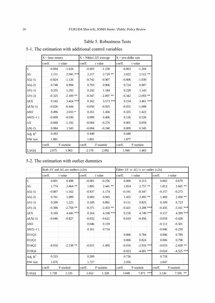
Table 5. Robustness Tests


C 0.001 0.498 -0.001 -0.256 0.000 0.313 0.002 0.679

∆G 1.774 2.464 ** 1.805 2.441 ** 1.814 2.757 ** 1.813 2.665 **

∆G(-1) -0.807 -1.162 -0.837 -1.174 -0.191 -0.347 -0.157 -0.273

∆G(-2) 0.761 1.089 0.683 0.945 1.425 2.495 ** 1.469 2.450 **

∆Y(-1) 0.209 1.225 0.169 0.881 0.111 0.825 0.109 0.723

∆Y(-2) -0.396 -2.758 ** -0.371 -2.453 ** -0.421 -3.208 *** -0.435 -3.161 ***

∆EX 0.169 4.445 *** 0.164 4.168 *** 0.156 4.749 *** 0.157 4.599 ***

∆EX(-1) -0.040 -0.827 -0.032 -0.621 -0.019 -0.456 -0.018 -0.428

∆Μ2 0.046 0.159 -0.112 -0.501

∆Μ2(−1) 0.161 0.716 -0.046 -0.250

D11Q3 0.006 0.784 0.006 0.789

D12Q1 0.006 0.824 0.006 0.798

D14Q2 -0.016 -2.238 ** -0.015 -1.495 -0.016 -2.916 *** -0.019 -2.439 **

D19Q4 -0.023 -4.681 *** -0.024 -4.525 ***

Adj. R2 0.533 0.509 0.736 0.718

DW stat 1.676 1.727 2.056 2.047


Σ∆G(i) 1.728 1.535 1.652 1.328 3.048 7.871 *** 3.126 7.595 **

Both ∆Y and ∆G are outliers (±2σ) Either ∆Y or ∆G is an outlier (±2σ)

5-2. The estimation with outlier dummies

coeff. t value coeff. t value coeff. t value

C -0.004 -1.634 -0.003 -1.238 -0.003 -1.204

∆G 2.151 2.945 *** 2.217 2.729 ** 2.022 2.512 **

∆G(-1) -0.824 -1.126 -0.742 -0.907 -0.806 -1.039

∆G(-2) 0.748 0.994 0.703 0.906 0.724 0.907

∆Y(-1) 0.255 1.292 0.242 1.184 0.228 1.143

∆Y(-2) -0.325 -2.109 ** -0.347 -2.097 ** -0.342 -2.093 **

∆EX 0.142 3.424 *** 0.162 3.573 *** 0.154 3.461 ***

∆EX(-1) -0.026 -0.444 -0.050 -0.935 -0.055 -1.008

∆Μ2 0.496 2.033 * 0.351 1.456 0.325 1.422

∆Μ2(−1) -0.009 -0.036 0.099 0.406 0.126 0.526

∆X -0.068 -1.192 -0.004 -0.276 0.001 0.059

∆X(-1) 0.084 1.543 -0.004 -0.240 0.009 0.345

Adj. R2 0.493 0.448 0.448

DW stat 1.881 1.801 1.877

coeff. F-statistic coeff. F-statistic coeff. F-statistic

Σ∆G(i) 2.075 1.963 2.178 2.092 1.940 1.483

X = yen-dollar rateX = base money X = Nikkei 225 average

5-1. The estimation with additional control variables


19

Table 5. Robustness Tests (continued)

Notes 1) *** = significant at the 1% level, ** = significant at the 5% level, and * = significant at the 10% level. 2) ΣΔG(i) shows the total effect including lags.

5-3. The estimation with further sample division


C 0.000 -0.091 -0.001 -0.424 -0.001 -0.204 0.000 -0.264

∆G 2.649 4.011 *** 2.461 2.555 * 2.660 1.871 * 1.197 1.239

∆G(-1) -0.230 -0.352 0.020 0.026 -1.038 -0.658 0.378 0.377

∆G(-2) 1.559 2.340 * 1.758 2.205 * -0.437 -0.270 1.732 1.652

∆Y(-1) 0.147 0.691 0.130 0.539 0.333 0.952 0.120 0.564

∆Y(-2) -0.527 -4.097 *** -0.547 -2.758 ** -0.116 -0.327 -0.206 -0.981

∆EX 0.165 4.219 *** 0.147 2.832 ** 0.097 0.808 0.190 2.578 **

∆EX(-1) -0.056 -0.847 -0.042 -0.578 -0.029 -0.266 0.079 1.097

D11Q3 0.004 0.473

D12Q1 0.006 0.653

D14Q2 -0.024 -3.410 ***

D19Q4 -0.024 -4.212 ***

Adj. R2 0.846 0.816 -0.037 0.634

DW stat 2.449 3.011 1.597 2.000


Σ∆G(i) 3.978 7.453 ** 4.239 6.869 * 1.185 0.185 3.306 3.237 *

2014Q2-2019Q42010Q4-2014Q1

5-4. The estimation with different benchmark year of GDP


C 0.000 -0.093 0.001 0.619 -0.002 -0.938 0.000 -0.160

∆G 1.551 1.976 * 0.985 1.612 3.451 2.447 ** 2.047 1.870 *

∆G(-1) -0.227 -0.304 -0.054 -0.099 -0.263 -0.320 -0.079 -0.137

∆G(-2) 0.668 0.831 0.933 1.612 1.412 1.436 1.212 1.849 *

∆Y(-1) 0.161 0.832 0.056 0.403 0.212 0.991 0.103 0.671

∆Y(-2) -0.206 -1.343 -0.284 -2.275 ** -0.328 -1.791 * -0.307 -2.302 **

∆EX 0.166 3.773 *** 0.165 4.693 *** 0.179 3.667 *** 0.166 4.451 ***

∆EX(-1) -0.086 -1.548 -0.023 -0.497 -0.083 -1.351 -0.030 -0.613

D11Q3 0.005 0.677 0.006 0.817

D12Q1 0.010 1.669 0.007 1.008

D14Q2 -0.020 -3.384 *** -0.016 -2.449 **

D19Q4 -0.022 -4.268 *** -0.023 -4.148 ***

Adj. R2 0.343 0.675 0.210 0.636

DW stat 1.622 1.913 1.776 2.149


Σ∆G(i) 1.991 1.705 1.864 2.814 4.601 4.111 * 3.179 3.919 *



was significantly positive at the 10% level, but the other control variables were not signifi-cant. Since the sample period was when the so-called “liquidity trap” occurred, the mone-tary policy of increasing the real money balance may have had little effect. In the estimation, the changes in stock prices and exchange rates had no consistent effect on the GDP due to large short-term volatility.

VI-3. Outlier dummy variables

In the following, we explore whether the result holds, despite removing the effects of outliers. In the analysis, we define ΔYt and ΔGt as outliers when they deviate from the aver-age of more than two standard deviations in the sample period from the fourth quarter of 2010 to that of 2019. This indicates that ΔYt is an outlier in the third quarter of 2011, the second quarter of 2014, and the fourth quarter of 2019 and that ΔGt is an outlier in the first quarter of 2012 and the second quarter of 2014. The third quarter of 2011 and the first quar-ter of 2012 coincided with the period of economic recovery after the Great East Japan Earth-quake. Contrarily, the second quarter of 2014 and the fourth quarter of 2019 reflect a con-sumption decline following the consumption tax hike.

To remove the effects of outliers, we considered two types of dummy variables. One is a dummy variable that takes one in the second quarter of 2014 when both ΔYt and ΔGt were outliers and zero otherwise. The others are three dummy variables, each of which takes one in the third quarter of 2011, the first quarter of 2012, and the fourth quarter of 2019, respec-tively, when either ΔYt or ΔGt was an outlier, and zero otherwise. We estimate Equation (1), either including the first type of dummy or including both types of dummies. The estimates were made with and without the growth rate of real money stock (M2) as an additional con-trol variable.

Table 5-2 reports the results of the least-squares method with outlier dummies. First, only with the dummy for the second quarter of 2014, the instantaneous impact (i.e. the esti-mated value of a0) ranged from approximately 1.77 to 1.81, and the total impact including lags (i.e. the estimated value of ∑2

i=0 ai ) ranged from approximately 1.65 to 1.73, both of which were significantly lower than without the outlier dummy. In the second quarter of 2014, both the GDP and government spending fell sharply. This may have overestimated the impact of government spending. However, even in the case where the value declined the most, both the instantaneous effect and the total effect, including lags, were greater in the estimates after than before the fourth quarter of 2010.

In contrast, with the dummies for the third quarter of 2011, the first quarter of 2012, the second quarter of 2014, and the fourth quarter of 2019, a similar decline was observed in the instantaneous effect. However, the effect of the two-period lag (i.e. the estimated value of a2) had a significant positive value, and consequently, the total impact including lags was approximately 3.05 to 3.13, which was larger than that without outlier dummies and more statistically significant. The existence of outliers might have biased the impact of fiscal spending on the GDP. However, even if we remove the effects of outliers, the impact of fis-


21

cal spending on the GDP increased significantly after the fourth quarter of 2010.

VI-4. Further structural breaks

In this subsection, we examine whether the results are valid when we further divide the sample period into the following periods: from the fourth quarter of 2010 to the first quarter of 2014, and from the second quarter of 2014 to the fourth quarter of 2019. Table 5-3 reports the results of estimation using the least-squares method for the two subdivided periods. We estimate with and without outlier dummies. A notable feature of the estimation results is that both the instantaneous effect and the total effect including lags were significantly larger in the first half (from the fourth quarter of 2010 to the first quarter of 2014) than in the entire period (from the fourth quarter of 2010 to the fourth quarter of 2019). Conversely, in the lat-ter half (from the second quarter of 2014 to the fourth quarter of 2019), the effect including lag dropped significantly when no outlier dummy was added, and the instantaneous impact dropped significantly when outlier dummies were added. The statistical significance also dropped substantially in the second half, with or without outlier dummies.

Since the sample size was very small, definitive conclusions should not be drawn from these results. However, the literal interpretation of these results suggests that the significant increase in the impact of fiscal spending on the GDP since the fourth quarter of 2010 mainly occurred before the first quarter of 2014, and the impact may not have been robust since the second quarter of 2014. This indicates that the “significant increase in the impact of fiscal spending since the fourth quarter of 2010” is not necessarily due to the ultra-low interest rate environment. This is because if the ultra-low interest rate environment increased the im-pact of fiscal spending, a larger value would be observed even after the second quarter of 2014, when long-term interest rates declined more significantly due to the strengthening of unconventional monetary policy.

VI-5. Alternative benchmark years for the GDP

In the following section, we examine whether the results are valid even when different methods and benchmark years of the GDP are used. In our previous analysis, we used data from the benchmark year 2011 (2008 SNA) published on November 16, 2020. This is be-cause the benchmark year 2011 (2008 SNA) was the latest available data from the first quar-ter of 1980 through the second quarter of 2020, when we made our initial estimations. How-ever, on December 8, 2020, data of the benchmark year 2015 (2008 SNA) were released, making updated data available from the first quarter of 1994 to the latest period. In this sec-tion, we use the benchmark year 2015 (2008 SNA) to check the robustness of our results.

The GDP statistics of the benchmark year 2015 use the 2008 SNA, which are similar to that of the benchmark year 2011. However, significant revisions have been made, such as the inclusion of renovations in investment, reflection of sales margins for condominiums, and updating of benchmarks for construction output estimates. Thus, not only did the level


of the GDP rise by about 1.3%, but the short-term fluctuations of GDP expenditures also changed significantly. For example, when examining the correlation coefficient between the value of the benchmark year 2011 and that of the benchmark year 2015 over the sample pe-riod from the fourth quarter of 2010 to the fourth quarter of 2019, the correlation coefficient was high at 0.975 for ΔYt but was not high at 0.836 for ΔGt. Furthermore, the correlation co-efficient between ΔYt and ΔGt, which was 0.421 in the benchmark year 2011, decreased sig-nificantly to 0.221 in the benchmark year 2015.

Table 5-4 summarizes the estimation results using the benchmark year 2015 (2008 SNA) and the least-squares method and the instrumental variable method, with and without outlier dummies. In the instrumental variable method, the constant term and the rate of increase in real exports were used as exogenous variables, and two-period lagged values of ΔYt, ΔGt, the growth rate of real private consumption, the growth rate of real private non-residential investment, and increase in real public investment/real GDP in the previous period were used as instrumental variables. The two-period lagged values in the rate of change in the Nikkei Stock Average and the yen-dollar exchange rate, along with the one-period lagged value in the rate of increase in real exports, were included as the instrumental variables.

The results of the least-squares method show that both the instantaneous effect and the total effect, including lags, were lower when using the benchmark year 2015 than when us-ing the benchmark year 2011. In particular, their statistical significance also declined when the benchmark year 2015 was used. Conversely, the results of the instrumental variable method show that both the instantaneous effect and the total effect, including lags, increased when using the benchmark year 2015. When using the benchmark year 2015, the negative correlation coefficient between ΔGt and the error term might have caused smaller estimates for both the instantaneous effect and the total effect, including lags, in the estimations by the least-squares method. However, these results indicate that the results may change signifi-cantly depending on the method and benchmark year of GDP, when assessing the impacts of fiscal spending.

VII. Analysis Based on the Forecast Survey Data

VII-1. Effects on GDP forecasts

Estimating the reduced-form equation and the VAR model, previous sections showed that the impact of fiscal spending on the GDP might have decreased over the medium-term but increased after the fourth quarter of 2010. In the following section, we examine whether this view is correct using forecast survey data from Japanese professional economists. Their forecast does not necessarily coincide with the actual effects of fiscal policy. However, it would be useful to see how Japan’s leading economists think about the effects of fiscal poli-cy under ultra-low interest rates.

The forecast survey data of economists used in the following analysis is based on “ESP Forecast,” which was collected by the Japan Center of Economic Research. It receives


23

monthly responses from approximately 40 private-sector economists who forecast several important indicators for the Japanese economy, including the GDP and its components6. The results of the survey revealed a consensus on future economic trends and economic sustain-ability. The real GDP growth rate, the real government consumption growth rate, and the real public investment growth rate in FY T are forecast monthly from October in FY T-2 to May in FY T + 17.

In the following analysis, we measure the “impact” of fiscal spending on the GDP by in-vestigating the extent to which individual forecasters change their GDP forecasts when they change their forecasts of government expenditures. Specifically, we estimate the following equation with a constant term using monthly forecaster-level panel data:

dEj,t ΔYT = ∑1i=0 αi dEj,t– jΔG1T +∑1

i=0 βi dEj,t– jΔG2T + γ dEj,t ΔEXT,j,t +υj +μT, (5)

Here, dEj,t represents a change in the forecast value of forecaster j from period t-1 to period t. ΔYT, ΔG1T, ΔG2T, and ΔEXT represent the growth rates of real GDP in FY T, the growth rate of real government consumption in FY T, the growth rate of real public investment in FY ΔT, and the growth rate of real exports in FY T, respectively8. νj and μT are the fixed effects for the forecaster and target year, respectively.

The dependent variable covers the forecasts from FY2009 to FY2019, during which the Japanese economy was experiencing ultra-low interest rates9. Estimates were made by pool-ing data not only for the period from FY2009 to FY2019 but also for the period after the Great East Japan Earthquake (i.e. from FY2013 to FY2019). If the entire period was pooled, ΔG1T, ΔG2T, and ΔEXT were estimated by adding the coefficient dummy in FY2011 to con-trol for the impact of the Great East Japan Earthquake.

Table 6 summarizes the estimation results. First, in the case of full-period estimations, the growth rates of real public investment and real exports had a significant positive effect on the growth rate of real GDP, regardless of the choice of the 2011 coefficient dummy. The growth rate of real government consumption also had a significant positive effect on the growth rate of real GDP when the coefficient dummy of 2011 was added. The results sug-gest that economists expected fiscal spending to impact economic growth, except in 2011. A positive effect was observed more robustly for public investment.

Conversely, in the FY2013 period, the growth rates of real government consumption, real public investment, and real exports had a significant positive effect on economic growth. In the forecasts formed after the Great East Japan Earthquake, economists expected the growth of government consumption and public investment to be more robustly correlat- 6 In April 2012, the Japan Center for Economic Research took over the Survey project that had been conducted by the Eco-nomic Planning Association since 2004. Fukuda and Soma (2019) analyzed the changes in inflation expectations under Abeno-mics using individual data from the survey.7 However, the forecast for growth rates for FY2009 and FY2010 will not be released until June in FY2008 and FY2009, re-spectively.8 For example, dEj,tΔYT represents how much the forecaster j changed his or her forecast of the real GDP growth rate in FY T from period t-1 to period t.9 The sample period is from FY2009 onwards, as the ESP forecast added the growth rate of government consumption and real public investment to the questionnaire from FY2009 onwards.


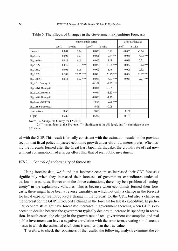
ed with the GDP. This result is broadly consistent with the estimation results in the previous section that fiscal policy impacted economic growth under ultra-low interest rates. When us-ing the forecasts formed after the Great East Japan Earthquake, the growth rate of real gov-ernment consumption had a larger effect than that of real public investment.

VII-2. Control of endogeneity of forecasts

Using forecast data, we found that Japanese economists increased their GDP forecasts significantly when they increased their forecasts of government expenditures under ul-tra-low interest rates. However, in the above estimations, there may be a problem of “endog-eneity” in the explanatory variables. This is because when economists formed their fore-casts, there might have been a reverse causality, in which not only a change in the forecast for fiscal expenditure introduced a change in the forecast for the GDP, but also a change in the forecast for the GDP introduced a change in the forecast for fiscal expenditure. In partic-ular, economists might have forecasted increases in government spending when GDP is ex-pected to decline because the government typically decides to increase its spending in reces-sion. In such cases, the change in the growth rate of real government consumption and real public investment can have a negative correlation with the error term, creating simultaneous biases in which the estimated coefficient is smaller than the true value.

Therefore, to check the robustness of the results, the following analysis examines the ef-

Table 6. The Effects of Changes in the Government Expenditure Forecasts

Notes 1) Dummy11≡Dummy for FY2011. 2) *** = significant at the 1% level, ** = significant at the 5% level, and * = significant at the 10% level.

coeff. t value coeff. t value coeff. t value

constant 0.004 0.24 0.003 0.21 -0.009 -0.64

dEj,t∆G1 T 0.002 0.93 0.051 2.54 ** 0.086 4.03 ***

dEj,t-1∆G1 T 0.011 1.08 0.018 1.48 0.011 0.71

dEj,t∆G2 T 0.017 6.63 *** 0.029 10.95 *** 0.022 8.44 ***

dEj,t-1∆G2 T 0.001 1.01 0.002 1.46 0.001 0.82

dEj,t∆EX T 0.102 20.25 *** 0.088 20.75 *** 0.092 23.67 ***

dEj,t-1∆EX T 0.011 3.52 *** 0.013 4.67 *** 0.019 7.21 ***

dEj,t∆G1·Dummy11 -0.101 -2.83 ***

dEj,t-1∆G1·Dummy11 -0.014 -0.59

dEj,t∆G2·Dummy11 -0.044 -8.33 ***

dEj,t-1∆G2·Dummy11 -0.005 -1.19

dEj,t∆EX·Dummy11 0.04 2.69 ***

dEj,t-1∆EX·Dummy11 -0.01 -0.99

observations 9055 9055 8131

Adj.R2 0.239 0.282 0.189

entire sample period after earthquake


25

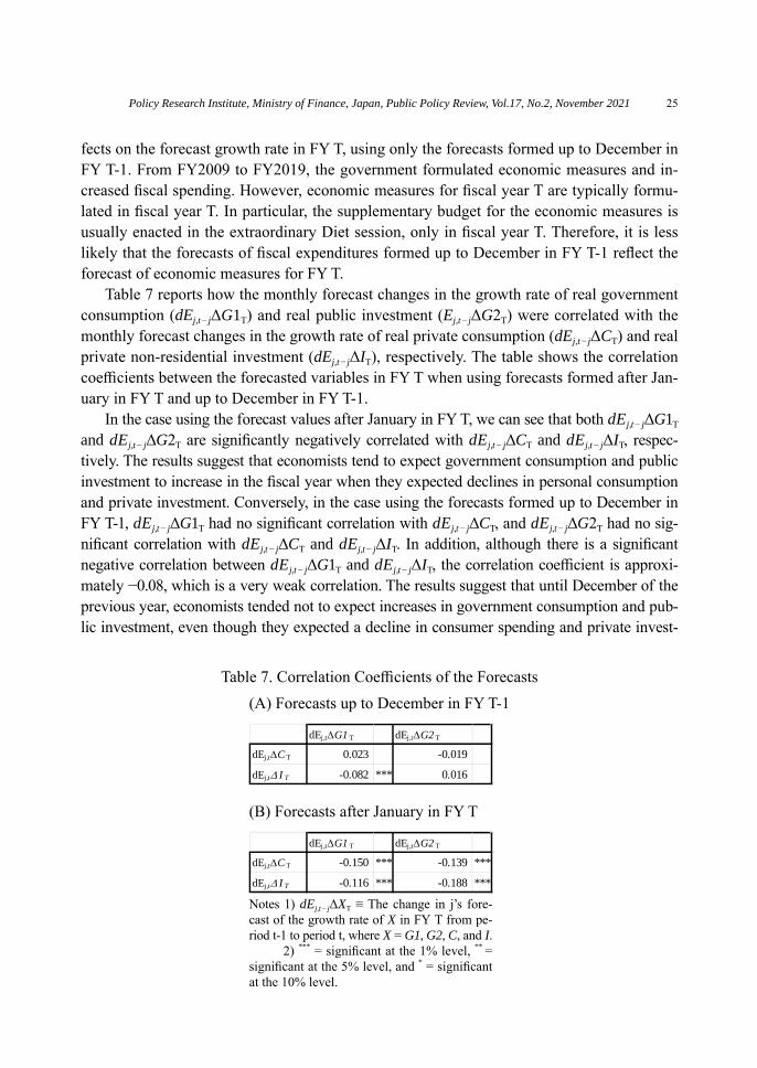
fects on the forecast growth rate in FY T, using only the forecasts formed up to December in FY T-1. From FY2009 to FY2019, the government formulated economic measures and in-creased fiscal spending. However, economic measures for fiscal year T are typically formu-lated in fiscal year T. In particular, the supplementary budget for the economic measures is usually enacted in the extraordinary Diet session, only in fiscal year T. Therefore, it is less likely that the forecasts of fiscal expenditures formed up to December in FY T-1 reflect the forecast of economic measures for FY T.

Table 7 reports how the monthly forecast changes in the growth rate of real government consumption (dEj,t− jΔG1T) and real public investment (Ej,t− jΔG2T) were correlated with the monthly forecast changes in the growth rate of real private consumption (dEj,t− jΔCT) and real private non-residential investment (dEj,t− jΔIT), respectively. The table shows the correlation coefficients between the forecasted variables in FY T when using forecasts formed after Jan-uary in FY T and up to December in FY T-1.

In the case using the forecast values after January in FY T, we can see that both dEj,t− jΔG1T and dEj,t− jΔG2T are significantly negatively correlated with dEj,t− jΔCT and dEj,t− jΔIT, respec-tively. The results suggest that economists tend to expect government consumption and public investment to increase in the fiscal year when they expected declines in personal consumption and private investment. Conversely, in the case using the forecasts formed up to December in FY T-1, dEj,t− jΔG1T had no significant correlation with dEj,t− jΔCT, and dEj,t− jΔG2T had no sig-nificant correlation with dEj,t− jΔCT and dEj,t − jΔIT. In addition, although there is a significant negative correlation between dEj,t − jΔG1T and dEj,t− jΔIT, the correlation coefficient is approxi-mately −0.08, which is a very weak correlation. The results suggest that until December of the previous year, economists tended not to expect increases in government consumption and pub-lic investment, even though they expected a decline in consumer spending and private invest-

Notes 1) dEj,t − jΔXT ≡ The change in j’s fore-cast of the growth rate of X in FY T from pe-riod t-1 to period t, where X = G1, G2, C, and I. 2) *** = significant at the 1% level, ** = significant at the 5% level, and * = significant at the 10% level.

Table 7. Correlation Coefficients of the Forecasts(A) Forecasts up to December in FY T-1

dEj,t∆G1 T dEj,t∆G2 T

dEj,t∆C T 0.023 -0.019

dEj,t∆ I T -0.082 *** 0.016

(B) Forecasts after January in FY T

dEj,t∆G1 T dEj,t∆G2 T

dEj,t∆C T -0.150 *** -0.139 ***

dEj,t∆ I T -0.116 *** -0.188 ***


ment in the next fiscal year. In other words, while there is a possibility of “simultaneity bias” in the estimation using the forecasts formed after January in FY T, it is less likely to occur us-ing the forecasts formed up to December in FY T-1.

Table 8 summarizes the estimation results of Equation (5) using only the forecasts formed up to December in FY T-110. In the table, both real government consumption and real public investment had a greater positive impact on the real GDP than that in Table 6. In particular, real government consumption had a much greater positive impact than that in Ta-ble 6. Despite controlling for the possibility of “simultaneous bias,” economists may have thought that fiscal spending was positively correlated with GDP under ultra-low interest rates. The estimation results are essentially the same when using the entire period and in the period after the Great East Japan Earthquake.

VIII. Concluding Remarks

In this study, we examined the effectiveness of macro-fiscal policy conceptually and re-considered its effectiveness by using data from 1980 onward. The sample period used in the analysis included the period of the “liquidity trap,” in which interest rates fell to zero or were negative. They also included the Abenomics period, in which a bold unconventional monetary policy was implemented. The results suggest that the impact of fiscal policy on the GDP may have decreased over the medium- to long-term period; however, the impact may have increased after the fourth quarter of 2010. It was also confirmed that private econo-mists considered fiscal spending to be significantly correlated with the GDP under extremely

Table 8. The Estimation by the Forecasts Formed up to December in FY T-1

Note: *** = significant at the 1% level, ** = significant at the 5% level, and * = significant at the 10% level.

coeff. t value coeff. t value

constant 0.014 0.69 0.015 0.71

dEj,t∆G1 T 0.110 2.87 *** 0.153 3.40 ***

dEj,t-1∆G1 T -0.003 -0.17 -0.011 -0.37

dEj,t∆G2 T 0.031 7.59 *** 0.027 5.98 ***

dEj,t-1∆G2 T 0.002 1.09 -0.002 -0.59

dEj,t∆EX T 0.091 9.67 *** 0.084 10.25 ***

dEj,t-1∆EX T 0.018 3.37 *** 0.012 2.57 ***

observations 3982 3180

Adj.R2 0.2253 0.174

entire sample period after earthquake

10 Unlike the case where all available forecasts are used, in the case where only forecasts formed up to December T-1 are used, all forecasts for FY2011 were formed before the Great East Japan Earthquake occurred. Therefore, ΔG1T and ΔG2T were esti-mated without the coefficient dummy of FY2011.


27

low interest rates.Nevertheless, it should be noted that the estimation of the reduced-form equation and

VAR model described in previous sections shows the “Granger causality,” which does not necessarily indicate a true causality. In addition, the results of this study do not imply that fiscal policy will continue to have a significant impact on the GDP even if the ultra-low in-terest rate environment continues. The estimated impacts of fiscal policy varied depending on the choice of outliers, the benchmark year of the GDP used, and the estimation period. In this sense, the results of this study must be interpreted with caution. Previous studies have long debated the effectiveness of fiscal policy. However, in the future, further verification will be necessary to confirm the robustness of these findings on the effectiveness of fiscal policy in Japan.

References

Andrews, D.W.K., (1993). “Tests for Parameter Instability and Structural Change with Un-known Change Point” Econometrica, 61(4), pp. 821-856.

Auerbach, A.J., and Y. Gorodnichenko, (2017). “Fiscal Multipliers in Japan” Research in Economics, 71(3), pp. 411-421.

Bessho, S., (2016). “Case Study of Central and Local Government Finance in Japan” Asian Development Bank Institute Working Paper Series No. 599 SSRN Electronic Journal.

Blanchard, O., (2019). “Public Debt and Low Interest Rates” American Economic Review, 109(4), pp. 1197-1229.

Bayoumi, T., (2001). “The Morning after: Explaining the Slowdown in Japanese Growth in the 1990s” Journal of International Economics, 53(2), pp. 241-259.

Brückner, M., and A. Tuladhar, (2014). “Local Government Spending Multipliers and Fi-nancial Distress: Evidence from Japanese Prefectures” The Economic Journal, 124(581), pp. 1279-1316.

Caballero, R.J., T. Hoshi, and A.K. Kashyap, (2008). “Zombie Lending and Depressed Re-structuring in Japan” American Economic Review, 98(5), pp. 1943-1977.

Fukuda, S., (2015). “Abenomics: Why was it so Successful in Changing Market Expecta-tions?” Journal of the Japanese and International Economies, 37, pp. 1-20.

Fukuda, S., and J. Nakamura, (2011). “Why Did ‘Zombie’ Firms Recover in Japan?” The World Economy, 34(7), pp. 1124-1137.

Fukuda, S., and J. Yamada, (2011). “Stock Price Targeting and Fiscal Deficit in Japan: Why Did the Fiscal Deficit Increase during Japan’s Lost Decades?” Journal of the Japanese and International Economies, 25(4), pp. 447-464.

Fukuda, S., and N. Soma, (2019). “Inflation Target and Anchor of Inflation Forecasts in Ja-pan” Journal of the Japanese and International Economies, 52, pp. 154-170.

Fukuda, S., and N. Soma, (2021), “Evaluation of Macro-Fiscal Policy and Challenges in Ja-pan” (in Japnanese), The Financial Review, No. 144, pp. 156-180.

Iwata, Y., (2011). “The Government Spending Multiplier and Fiscal Financing: Insights


from Japan” International Finance, 14(2), pp. 231-264.Kameda, T., R. Namba, and T. Tsuruga, (2021). “Decomposing Local Fiscal Multipliers:

Evidence from Japan” Japan and the World Economy, 57, article 101053.Kato, A., W. Miyamoto, T.L. Nguyen, and D. Sergeyev, (2018). “The Effects of Tax Chang-

es at the Zero Lower Bound: Evidence from Japan,” AEA Papers and Proceedings, 108, pp. 513-518.

Kuttner, K.N., and A.S. Posen, (2001). “The Great Recession: Lessons for Macroeconomic Policy from Japan” Brookings Papers on Economic Activity, 2001(2), pp. 93-185.

Kuttner, K.N., and A.S. Posen, (2002). “Fiscal Policy Effectiveness in Japan” Journal of the Japanese and International Economies, 16(4), pp. 536-558.

Miyamoto, W., T.L. Nguyen, and D. Sergeyev, (2018). “Government Spending Multipliers under the Zero Lower Bound: Evidence from Japan” American Economic Journal: Macroeconomics, 10(3), pp. 247-277.

Morita, H. (2015). “Japanese Fiscal Policy under the Zero Lower Bound of Nominal Interest Rates: Time-varying Parameters Vector Autoregression,” IER Discussion Paper A No. 627, Hitotsubashi University.

Umeda, M., T. Kawamoto, and M. Hori, (2018). “Twin Survey on the Japanese Economy and Policy Effects: Outline of the Survey and Report of Summary Statistics” Economic Analysis, 197, pp. 144-185.

Werner, R. (2004). “Why has Fiscal Policy Disappointed in Japan?” Money Macro and Fi-nance (MMF) Research Group Conference 2004 9, Money Macro and Finance Re-search Group.

Yoshino, N., and H. Miyamoto, (2017). “Declined Effectiveness of Fiscal and Monetary Policies Faced with Aging Population in Japan” Japan and the World Economy, 42, pp. 32-44.


evaluation of japan’s macro-fiscal policy and its challenges

Documents