evaluation of flow models and pollutant retention …gala.gre.ac.uk/14319/1/ruth_quinn_2015.pdf ·...
TRANSCRIPT

EVALUATION OF FLOW
MODELS AND
POLLUTANT RETENTION
ISOTHERMS FOR THEIR
APPLICATION TO RAIN
GARDEN BIORETENTION
Ruth Quinn
A thesis submitted in partial fulfilment of the
requirements of the University of Greenwich for the
Degree of Doctor of Philosophy

Design of SuDS: A Modelling Tool 2015
i | P a g e
DECLARATION
“I certify that this work has not been accepted in substance for any degree, and is
not concurrently being submitted for any degree other than that of Doctor of Philosophy
being studied at the University of
Greenwich. I also declare that this work is the result of my own investigations except
where otherwise identified by references and that I have not plagiarised the work of
others”.
Ruth Quinn
Candidate
Supported by
Peter Kyberd
Head of Engineering Science

Design of SuDS: A Modelling Tool 2015
ii | P a g e
ACKNOWLEDGEMENTS
Firstly, I would like to express my gratitude to my supervisor Dr. Alejandro Dussaillant for his
contributions to my research. I also wish to thank my second supervisor Prof Amir Alani for
his advice and support during my Ph.D. study.
Besides my advisors, I would like to thank my thesis committee: Prof Sue Charlesworth and
Prof Colin Hills for their suggestions, encouragement and support.
My sincere thanks also goes to the staff at the school of engineering especially the laboratory
staff and technicians: Ian Cakebread, Tony Stevens, Bruce Hassan, Colin Gordon and Matthew
Bunting whose help and assistance was invaluable. Without their support it would not have
been possible to conduct this research.
I would also like to thank the head of Engineering and Deputy Pro-Vice Chancellor Prof
Simeon Keates for his advice and understanding.
Last but not least, I would like to thank my parents, Peter and Elizabeth, my brother, Cillian,
my boyfriend Jeff and all of my friends for supporting me throughout writing this thesis and
my life in general.

Design of SuDS: A Modelling Tool 2015
iii | P a g e
ABSTRACT The primary aims of this research was firstly to develop a computer modelling tool which could
predict pollution retention in a rain garden and secondly to use the model and additional
experiments to examine various aspects of rain garden design with respect to pollutant
retention.
Initially, the behaviour of all contaminants in urban runoff was examined including their
retention and possible modelling methods. Heavy metals were then identified as the main focus
of this project as this choice was the most beneficial addition to current research. The main
factors affecting their retention were found to be macropore flow, pore water velocity, soil
moisture content and soil characteristics and the primary method of modelling capture was
identified as a sorption isotherm. Thus a dual-permeability heavy metal sorption model was
developed; this was based on an intensive literature review of current best practice in both
hydrological modelling and pollutant retention fields with respect to rain garden devices.
The kinematic wave equation was chosen to model water movement in both the matrix and
macropore regions as this provided a simpler alternative to more complex equations while still
maintaining good accuracy. With regards to the modelling of heavy metal retention three
isotherms were chosen: the linear, Langmuir and Freundlich equations as these were found
from previous research to be the most accurate. These isotherms were incorporated into a one
dimensional advection-dispersion-adsorption equation in order to model both transport and
retention together.
This model was tested against the appropriate literature and accurate comparisons were
obtained thus validating it.
Column experiments were designed to both provide a unique contribution to rain garden
research and further validate the model. This was achieved by analysing past experiments and
identifying an area where research is lacking; this area was the effect of macropore flow on
heavy metal retention in rain garden systems under typical English climatic conditions. The
findings of these experiments indicated that although macropore flow did not impact the
hydraulic performance of the columns, retention of the most mobile of heavy metals, copper,
was decreased slightly in one case. The overall retention of the columns was still high however
at a value in excess of 99% for copper, lead and zinc. The results of the experiments were also
used to further validate the model.

Design of SuDS: A Modelling Tool 2015
iv | P a g e
The model was then applied to the development of a rain garden device for a planned
roundabout in Kent, U.K. Preliminary design considered an upper root zone layer with organic
soil and a sandy storage sublayer each 30 cm thick, for a rain garden area of 5 and 10% the size
of the contributing impervious surface. Two scenarios were examined; the accumulation and
movement of metals without macropores and the possibility of groundwater contamination due
to preferential flow. It was shown that levels of lead can build up in the upper layers of the
system, but only constituted a health hazard after 10 years. Simulations showed that copper
was successfully retained (no significant concentrations below 50 cm of rain garden soil depth).
Finally given concerns of preferential flow bypassing sustainable drainage systems, macropore
flow was examined; results indicated that due to site conditions it was not a threat to
groundwater at this location for the time frame considered.
These actions successfully completed the objectives of this project and it was deemed
successful.

Design of SuDS: A Modelling Tool 2015
v | P a g e
CONTENTS DECLARATION ........................................................................................................................ i
ACKNOWLEDGEMENTS ....................................................................................................... ii
ABSTRACT ............................................................................................................................. iii
LIST OF FIGURES ................................................................................................................... x
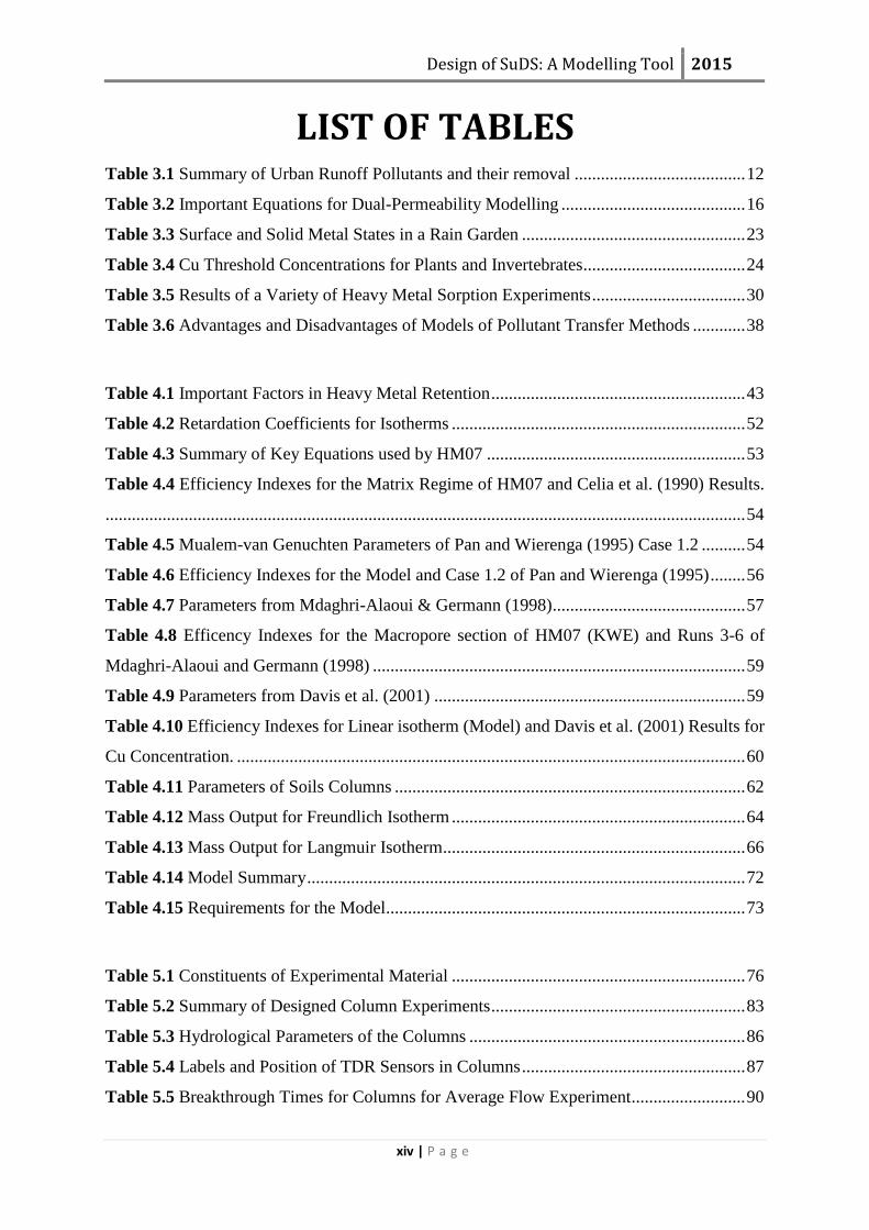
LIST OF TABLES .................................................................................................................. xiv
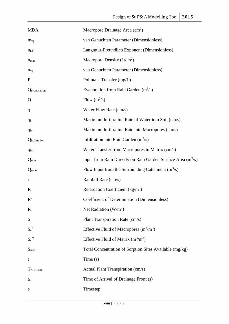
LIST OF SYMBOLS .............................................................................................................. xvi
ACROYNMS .......................................................................................................................... xxi
1 INTRODUCTION .............................................................................................................. 1
1.1 Background to Research.............................................................................................. 1
1.2 Justification ................................................................................................................. 3
1.3 Research Aims............................................................................................................. 4
1.4 Report Outline ............................................................................................................. 5
1.5 Conclusion ................................................................................................................... 6
2 METHODOLOGY ............................................................................................................. 7
2.1 Introduction ................................................................................................................. 7
2.2 Stage 1 - Identification of Key Factors ....................................................................... 7
2.3 Stage 2 - Development and Design of the Model ....................................................... 8
2.4 Stage 3 - Verification of the Model ............................................................................. 8
2.5 Stage 4 - Design and Complete Column Experiments ................................................ 9
2.6 Stage 5 - Perform Simulations .................................................................................... 9
3 LITERATURE REVIEW ................................................................................................. 10
3.1 Introduction ............................................................................................................... 10
3.2 Groundwater Recharge .............................................................................................. 10
3.3 Urban Runoff Contaminants ..................................................................................... 11
3.4 Water Modelling ....................................................................................................... 15
3.4.1 Dual Permeability Water Modelling .................................................................. 15
3.4.2 Evapotranspiration ............................................................................................. 20

Design of SuDS: A Modelling Tool 2015
vi | P a g e
3.4.3 Conclusions on Water Modelling ...................................................................... 21
3.5 Heavy Metal Adsorption ........................................................................................... 21
3.5.1 Cu ....................................................................................................................... 23
3.5.2 Pb ....................................................................................................................... 24
3.5.3 Zn ....................................................................................................................... 25
3.5.4 Heavy Metal Fractions ....................................................................................... 26
3.5.5 Sorption Experiments......................................................................................... 28
3.5.6 Linear Isotherm .................................................................................................. 31
3.5.7 Langmuir Isotherm model.................................................................................. 31
3.5.8 Freundlich Isotherm ........................................................................................... 32
3.5.9 Sips Isotherm ..................................................................................................... 33
3.5.10 Other Impacting Factors on Heavy Metal Retention ......................................... 33
3.5.11 Conclusions ........................................................................................................ 35
3.6 Heavy Metal Transport and Retention ...................................................................... 36
3.6.1 Transport and Retention in the Matrix Region .................................................. 36
3.6.2 Transport and Retention in the Macropore Region............................................ 41
3.6.3 Pollutant Transfer............................................................................................... 41
3.6.4 Conclusions ........................................................................................................ 41
3.7 Summary ................................................................................................................... 42
4 MODEL DEVELOPMENT ............................................................................................. 43
4.1 Introduction ............................................................................................................... 43
4.2 Hydrological Component .......................................................................................... 44
4.2.1 Matrix Region .................................................................................................... 44
4.2.2 Macropore Region ............................................................................................. 47
4.3 Pollutant Retention Component ................................................................................ 50
4.3.1 Heavy Metal Transport Modelling..................................................................... 50
4.3.2 Advection-Dispersion-Adsorption Equation ..................................................... 51
4.4 Preliminary Validation .............................................................................................. 52
4.4.1 Matrix Region .................................................................................................... 53
4.4.2 Macropore Region Flow .................................................................................... 56
4.4.3 Pollutant Retention (Linear Isotherm) ............................................................... 59

Design of SuDS: A Modelling Tool 2015
vii | P a g e
4.4.4 Pollutant Retention (Langmuir and Freundlich Isotherms) ............................... 60
4.5 Conclusion ................................................................................................................. 71
5 COLUMN EXPERIMENTS:
DESIGN AND RESULTS ....................................................................................................... 74
5.1 Introduction ............................................................................................................... 74
5.2 Aim of Column Experiments .................................................................................... 74
5.3 Column Experimental Design ................................................................................... 75
5.3.1 Composition & Macropore Presence ................................................................. 75
5.3.2 Input Metals ....................................................................................................... 77
5.3.3 Conditions .......................................................................................................... 78
5.3.4 Instrumentation .................................................................................................. 79
5.3.5 Calibration of Instrumentation ........................................................................... 81
5.3.6 Programming...................................................................................................... 82
5.3.7 Tracer ................................................................................................................. 82
5.3.8 Summary ............................................................................................................ 82
5.4 Methodology ............................................................................................................. 84
5.4.1 Average Flow Experiment ................................................................................. 85
5.4.2 First Flush Experiment ....................................................................................... 85
5.4.3 Heavy Metal Testing .......................................................................................... 86
5.5 Results ....................................................................................................................... 86
5.5.1 Hydrological Results for Experimental Set 1 .................................................... 86
5.5.2 Heavy Metal Results for Experimental Set 1 ..................................................... 92
5.6 Statistical Analysis of Heavy Metal Results ............................................................. 96
5.6.1 T-test (P-value) .................................................................................................. 98
5.6.2 ANOVA concept .............................................................................................. 106
5.7 Results of Further Experiments ............................................................................... 108
5.7.1 Experimental Set 2 ........................................................................................... 108
5.7.2 Experimental Set 3 ........................................................................................... 113
5.8 Comparisons Between Experimental Sets............................................................... 117
5.8.1 Average Flow Runs.......................................................................................... 117
5.8.2 First Flush Runs ............................................................................................... 119

Design of SuDS: A Modelling Tool 2015
viii | P a g e
5.9 Conclusion and Discussion ..................................................................................... 121
6 COLUMN EXPERIMENT: VALIDATION ........................................................... 124
6.1 Introduction ............................................................................................................. 124
6.2 Van Genuchten Parameters ..................................................................................... 124
6.3 Derivation of Unsaturated Hydraulic Conductivity ................................................ 126
6.4 Validation of Water Component of Model ............................................................. 129
6.5 Heavy Metal Retention Validation .......................................................................... 135
6.6 Conclusions ............................................................................................................. 137
7 MODEL APPLICATION ............................................................................................... 138
7.1 Introduction ............................................................................................................. 138
7.2 Site Description ....................................................................................................... 140
7.3 Accumulation and Transfer without Macropores.................................................... 142
7.4 Macropore flow ....................................................................................................... 143
7.5 Results ..................................................................................................................... 144
7.5.1 Matrix Flow ..................................................................................................... 144
7.5.2 Macropore Flow ............................................................................................... 148
7.5.3 Sensitivity Analysis ......................................................................................... 149
7.6 Discussion ............................................................................................................... 150
8 DISCUSSION ................................................................................................................. 153
8.1 Introduction ............................................................................................................. 153
8.2 Application of the Model ........................................................................................ 153
8.2.1 Rain Gardens .................................................................................................... 153
8.2.2 Green Roofs ..................................................................................................... 154
8.2.3 Permeable Pavements ...................................................................................... 156
8.3 Advantages of the Model ........................................................................................ 157
8.4 Limitations .............................................................................................................. 158
8.5 Contribution to Knowledge ..................................................................................... 158
8.5.1 Model ............................................................................................................... 158

Design of SuDS: A Modelling Tool 2015
ix | P a g e
8.5.2 Experimental .................................................................................................... 159
8.5.3 Simulations ...................................................................................................... 159
9 CONCLUSION AND FURTHER WORK .................................................................... 160
9.1 Introduction ............................................................................................................. 160
9.2 Conclusions ............................................................................................................. 160
9.3 Further Work and Recommendations ..................................................................... 165
REFERENCES ...................................................................................................................... 167
A DUAL-PERMEABILITY MODELS……………………………………………….183
B DISCRETIZATION OF KEY EQUATIONS………………………………………190
C EXPERIMENTAL DESIGN………………………………………………………..201
D EXPERIMENTAL RESULTS……………………………………………………...207
E PUBLICATIONS AND CONFERENCES ATTENDED…………………………..247

Design of SuDS: A Modelling Tool 2015
x | P a g e
LIST OF FIGURES Figure 1.1 Hourly Rainfall Intensity as a Percentage of Total Precipitation at Heathrow Airport
.................................................................................................................................................... 2
Figure 1.2 Diagram of a Rain Garden. Adapted from TP (2014) ............................................. 3
Figure 2.1 Five Stage Methodology .......................................................................................... 7
Figure 3.1 Heavy Metal Behaviour in Soil ............................................................................. 22
Figure 4.1 Relationship Between Near-Surface and Maximum Soil Profile Conductance
Parameters and Conductance (b). Adapted from Buttle and McDonald (2000). ..................... 49
Figure 4.2 Comparison of KWE Results with Celia et al. (1990) Simulation. ....................... 53
Figure 4.3 Comparison of the Results from KWE Model with Layered Soil Simulation with
case 1.2 Pan & Wierenga (1995). ............................................................................................ 55
Figure 4.4 Comparison of KWE with Cases 3-6 in Mdaghri-Alaoui and Germann (1998) ... 58
Figure 4.5 Comparison of Linear Isotherm (Model) Results for Cu Retention to Experiments
of Davis et al. (2001) ............................................................................................................... 60
Figure 4.6 Comparison of Freundlich Isotherm with the Outflow of Cu Concentration from
Column 1 (Oolitic Soils) .......................................................................................................... 63
Figure 4.7 Comparison of Freundlich Isotherm with the Outflow Zn Concentration from Lower
Greensand Aquifer ................................................................................................................... 64
Figure 4.8 Comparison of Langmuir Isotherm with the Outflow Cu Concentration from Oolitic
Soils.......................................................................................................................................... 65
Figure 4.9 Comparison of Langmuir Isotherm with the Outflow Zn Concentration from Lower
Greensand Aquifer ................................................................................................................... 65
Figure 4.10 Sensitivity Analysis of Pore Water Velocity on Freundlich Isotherm Results for
Cu Column 1 (Oolitic soils) ..................................................................................................... 67
Figure 4.11 Sensitivity Analysis of Pore Water Velocity on Freundlich Isotherm Results for
Zn Column 11 (Lower Greensand Aquifer)............................................................................. 68
Figure 4.12 Sensitivity Analysis of Bulk Density on Freundlich Isotherm Results for Cu
Column 1 (Oolitic Soil) ........................................................................................................... 69

Design of SuDS: A Modelling Tool 2015
xi | P a g e
Figure 4.13 Sensitivity Analysis of Bulk Density on Freundlich Isotherm for Zn Column 11
(Lower Greensand Aquifer) ..................................................................................................... 69
Figure 4.14 Sensitivity Analysis of Porosity on Freundlich Isotherm for Column 11 (Lower
Greensand Aquifer) .................................................................................................................. 70
Figure 4.15 Flow Chart of Model ........................................................................................... 71
Figure 5.1 Hourly Rainfall at Heathrow Weather Station from 1998-2008 ........................... 78
Figure 5.2 Hourly rainfall (mm) at Heathrow from 13/10/04 to 14/10/04 ............................. 79
Figure 5.3 Diagram of Column Experiments. All units in mm............................................... 81
Figure 5.4 Experimental Layout ............................................................................................. 84
Figure 5.5 Comparison of Soil Moisture Content in Column 2 (Matrix) and Column 5
(Macropore). Run 3. ................................................................................................................. 88
Figure 5.6 Comparison of Soil Moisture Content in Column 2 (Matrix) and Column 1
(Macropore). Run 3. ................................................................................................................. 89
Figure 5.7 Comparison of Soil Moisture Content in Column 2 (Matrix) and Column 5
(Macropore). First Flush. ......................................................................................................... 91
Figure 5.8 Cu Outflow Results ............................................................................................... 94
Figure 5.9 Pb Outflow Results ................................................................................................ 94
Figure 5.10 Zn Outflow Results .............................................................................................. 95
Figure 5.11 Plot of Cu Outflow Mean for the Different Columns. ......................................... 96
Figure 5.12 Plot of Pb Outflow Mean for the Different Columns. ......................................... 97
Figure 5.13 Plot of Zn Outflow Mean for the Different Columns. ......................................... 97
Figure 5.14 Cu Outflow Results for Experimental Set 2 ...................................................... 109
Figure 5.15 Pb Outflow Results for Experimental Set 2....................................................... 110
Figure 5.16 Zn Outflow Results for Experimental Set 2 ...................................................... 111
Figure 5.17 Plot of Cu Outflow Mean for the Different Columns for Experimental Set 2 .. 111
Figure 5.18 Plot of Pb Outflow Mean for the Different Columns for Experimental Set 2 ... 112
Figure 5.19 Plot of Zn Outflow Mean for the Different Columns for Experimental Set 2 ... 112
Figure 5.20 Cu Outflow Concentration for Experimental Set 3 ........................................... 114
Figure 5.21 Pb Outflow Concentration for Experimental Set 3 with Outliers ...................... 114
Figure 5.22 Pb Outflow Concentration for Experimental Set 3 without Outliers................. 115
Figure 5.23 Zn Outflow Concentration for Experimental Set 3 ........................................... 115
Figure 5.24 Plot of Cu Outflow Mean for the Different Columns for Experimental Set 3 .. 116

Design of SuDS: A Modelling Tool 2015
xii | P a g e
Figure 5.25 Plot of Zn Outflow Mean for the Different Columns for Experimental Set 3 ... 116
Figure 5.26 Plot of Pb Outflow Mean for the Different Columns for Experimental Set 3 with
Outliers ................................................................................................................................... 117
Figure 5.27 Comparison of Outflow Cu Concentration in Column 1 for Different Experimental
Sets for Average Flow Runs. ................................................................................................. 118
Figure 5.28 Comparison of Outflow Pb Concentration in Column 2 for Different Experimental
Sets for Average Flow Runs. ................................................................................................. 118
Figure 5.29 Comparison of Outflow Zn Concentration in Column 5 for Different Experimental
Sets for Average Flow Runs. ................................................................................................. 119
Figure 5.30 Comparison of Outflow Cu Concentration in Column 3 for Different Experimental
Sets for First Flush Flow Runs. ............................................................................................. 120
Figure 5.31 Comparison of Outflow Pb Concentration in Column 3 for Different Experimental
Sets for First Flush Flow Runs. ............................................................................................. 120
Figure 5.32 Comparison of Outflow Zn Concentration in Column 3 for Different Experimental
Sets for First Flush Flow Runs. ............................................................................................. 121
Figure 6.1 Comparison of Water Retention Curve for Soil/Sand Mix with the Van Genuchten
Fit. .......................................................................................................................................... 125
Figure 6.2 Comparison of Water Retention Curve for Sand with the Van Genuchten Fit. .. 126
Figure 6.3 Derived Unsaturated Hydraulic Conductivity for Column 1. Average Flow Run.
................................................................................................................................................ 128
Figure 6.4 Derived Unsaturated Hydraulic Conductivity for Column 1. First Flush Run. ... 129
Figure 6.5 Comparison of Experimental Soil Moisture Content at z=15cm with Kinematic
Wave Equation for Average Flow Condition ........................................................................ 131
Figure 6.6 Comparison of Experimental Soil Moisture Content at z=55cm with Kinematic
Wave Equation for Average Flow Condition ........................................................................ 131
Figure 6.7 Comparison of Experimental Soil Moisture Content at z=75cm with Kinematic
Wave Equation for Average Flow Condition ........................................................................ 132
Figure 6.8 Comparison of Experimental Soil Moisture Content at z=10cm with Kinematic
Wave Equation for First Flush Flow Condition ..................................................................... 133
Figure 6.9 Comparison of Experimental Soil Moisture Content at z=55cm with Kinematic
Wave Equation for First Flush Flow Condition ..................................................................... 134

Design of SuDS: A Modelling Tool 2015
xiii | P a g e
Figure 6.10 Comparison of Experimental Soil Moisture Content at z=75cm with Kinematic
Wave Equation for First Flow Condition............................................................................... 134
Figure 6.11 Comparison of Linear Isotherm with Experimental Results for Cu. ................. 136
Figure 6.12 Comparison of Linear Isotherm with Experimental Results for Pb. ................. 136
Figure 6.13 Comparison of Linear Isotherm with Experimental Results for Zn. ................. 137
Figure 7.1 Site Location Plan of Rain Garden ...................................................................... 138
Figure 7.2 Existing Site Layout ............................................................................................ 139
Figure 7.3 Proposed Site Layout ........................................................................................... 140
Figure 7.4 Diagram of Rain Garden Device ......................................................................... 141
Figure 7.5 Pb2+ Concentration in Rain Garden Soil with Highly Retentive (Organically-
Enriched) Soil (Kd=171214 L/kg) and Lower Retentive (Standard) Topsoil (Kd=500 L/kg) and
Two Area Ratios. ................................................................................................................... 145
Figure 7.6 Pb2+ Concentration in Water for Lower Retentive Topsoil with a 5% Area Ratio
after 10 years. ......................................................................................................................... 146
Figure 7.7 Cu2+ Concentration in Soil-Water for Highly Retentive (Organically Enriched) Soil
and Two Area Ratios after 10 Years. ..................................................................................... 147
Figure 7.8 Cu2+ Concentration in Water for High (Kd=4799 L/kg) and Lower Retentive
(Kd=550 L/kg) Soil with a 5% Area Ratio after 10 Years. .................................................... 147
Figure 7.9 Cu2+ Concentration in Macropore Water for Highly Retentive (Organically
Enriched) Soil and Two Area Ratios after 10 Years. ............................................................. 148
Figure 7.10 Cu2+ Water Concentration in Macropore Water for Lower Retentive Topsoil and
Two Area Ratios. ................................................................................................................... 149
Figure 7.11 Sensitivity Analysis ........................................................................................... 150
Figure 8.1 Diagram of a Permeable Pavement (Scholz & Grabowiecki, 2007) ................... 156
Design of SuDS: A Modelling Tool 2015
xiv | P a g e
LIST OF TABLES Table 3.1 Summary of Urban Runoff Pollutants and their removal ....................................... 12
Table 3.2 Important Equations for Dual-Permeability Modelling .......................................... 16
Table 3.3 Surface and Solid Metal States in a Rain Garden ................................................... 23
Table 3.4 Cu Threshold Concentrations for Plants and Invertebrates..................................... 24
Table 3.5 Results of a Variety of Heavy Metal Sorption Experiments ................................... 30
Table 3.6 Advantages and Disadvantages of Models of Pollutant Transfer Methods ............ 38
Table 4.1 Important Factors in Heavy Metal Retention .......................................................... 43
Table 4.2 Retardation Coefficients for Isotherms ................................................................... 52
Table 4.3 Summary of Key Equations used by HM07 ........................................................... 53
Table 4.4 Efficiency Indexes for the Matrix Regime of HM07 and Celia et al. (1990) Results.
.................................................................................................................................................. 54
Table 4.5 Mualem-van Genuchten Parameters of Pan and Wierenga (1995) Case 1.2 .......... 54
Table 4.6 Efficiency Indexes for the Model and Case 1.2 of Pan and Wierenga (1995) ........ 56
Table 4.7 Parameters from Mdaghri-Alaoui & Germann (1998) ............................................ 57
Table 4.8 Efficency Indexes for the Macropore section of HM07 (KWE) and Runs 3-6 of
Mdaghri-Alaoui and Germann (1998) ..................................................................................... 59
Table 4.9 Parameters from Davis et al. (2001) ....................................................................... 59
Table 4.10 Efficiency Indexes for Linear isotherm (Model) and Davis et al. (2001) Results for
Cu Concentration. .................................................................................................................... 60
Table 4.11 Parameters of Soils Columns ................................................................................ 62
Table 4.12 Mass Output for Freundlich Isotherm ................................................................... 64
Table 4.13 Mass Output for Langmuir Isotherm ..................................................................... 66
Table 4.14 Model Summary .................................................................................................... 72
Table 4.15 Requirements for the Model.................................................................................. 73
Table 5.1 Constituents of Experimental Material ................................................................... 76
Table 5.2 Summary of Designed Column Experiments .......................................................... 83
Table 5.3 Hydrological Parameters of the Columns ............................................................... 86
Table 5.4 Labels and Position of TDR Sensors in Columns ................................................... 87
Table 5.5 Breakthrough Times for Columns for Average Flow Experiment.......................... 90

Design of SuDS: A Modelling Tool 2015
xv | P a g e
Table 5.6 Breakthrough Times for Columns for First Flush Experiment ............................... 91
Table 5.7 Blank Sample Range and Average for Experimental Set 1 .................................... 93
Table 5.8 Initial Conditions for Each of the Average Flow Experimental Runs .................... 93
Table 5.9 P-values for Experimental Runs for Cu. ................................................................. 99
Table 5.10 P-values for Experimental Runs for Pb. .............................................................. 100
Table 5.11 P-values for Experimental Runs for Zn. ............................................................. 101
Table 5.12 P-values for Columns with Similar Characteristics for Cu ................................. 102
Table 5.13 P-values for Columns with Different Characteristics for Cu .............................. 103
Table 5.14 P-values for Columns with Similar Characteristics for Pb ................................. 104
Table 5.15 P-values for Columns with Different Characteristics for Pb .............................. 104
Table 5.16 P-values for Columns with Similar Characteristics for Zn ................................. 105
Table 5.17 P-values for Columns with Different Characteristics for Zn .............................. 105
Table 5.18 Two Way ANOVA Analysis Results for Cu Outflow ........................................ 106
Table 5.19 Two Way ANOVA Analysis Results for Pb Outflow ........................................ 106
Table 5.20 Two Way ANOVA Analysis Results for Zn Outflow ........................................ 107
Table 5.21 Two Way ANOVA Analysis for Pb Outflow for Three Runs\ ........................... 107
Table 5.22 Two Way ANOVA Analysis for Zn Outflow for Three Runs ............................ 108
Table 5.23 Blank Sample Range and Average for Experimental Set 2 ................................ 109
Table 5.24 Blank Sample Range and Average for Experimental Set 3 ................................ 113
Table 6.1 Van Genuchten Parameters for Column 1 Sand/Soil Mix .................................... 125
Table 6.2 Van Genuchten Parameters for Column 1 Sand ................................................... 126
Table 6.3 Initial and Boundary Conditions For Average Flow Experiment ......................... 130
Table 6.4 Initial and Boundary Conditions for First Flush Experiment................................ 133
Table 6.5 Linear Distribution Coefficients for Experimental Substrates .............................. 135
Table 7.1 Hydraulic Parameters of the Rain Garden ............................................................ 141
Table 7.2 Heavy Metal Retention Parameters of the Soil ..................................................... 143
Table 8.1 Heavy Metal Concentrations in Rainfall ............................................................... 154

Design of SuDS: A Modelling Tool 2015
xvi | P a g e
LIST OF SYMBOLS A Area Ratio (%)
aF Freundlich Exponent (Dimensionless)
aLF Langmuir-Freundlich Exponent (Dimensionless)
am Macropore Exponent (Dimensionless)
Arg Area of Rain Garden (cm2)
bm Conductance of Macropores (cm/s)
c Kinematic Wave Celerity (cm/s)
C Dissolved Pollutant Concentration (mg/L)
CA Cross Sectional Area (m2)
cD Drainage Celerity (cm/s)
Ce Effluent Metal Level (mg/L)
cm Macropore Celerity (cm/s)
Cma Pollutant Concentration in Macropore (mg/L)
Cmi Pollutant Concentration in Matrix (mg/L)
Co Influent Metal Level (mg/L)
Cs Media-sorbed Pollutant (mg/kg)
cw Wetting Front Celerity (cm/s)
D Dispersion Coefficient (cm2/s)
d Dispersity (cm)
De Effective Diffusion Coefficient (cm2/s)
Dm Mechanical Dispersion (cm2/s)
Do Binary Diffusion Coefficient (cm2/s)
dp Effective ‘Diffusion’ Pathlength (cm)
dr Drainage Rate (cm/s)
Eactual Actual Evaporation (cm/s)

Design of SuDS: A Modelling Tool 2015
xvii | P a g e
ee Molecular Diffusion (cm2/s)
Ep Potential Evaporation (cm)
Es Potential Soil Evaporation (cm/s)
F Infiltration (cm)
G Soil Heat Density (W/m2)
Gf Geometry Factor (Dimensionless)
h Pressure Head (cm)
hb Head at Bottom Boundary (cm)
hd Depression Depth of Rain Garden (cm)
hf Pressure Head in the Macropore (cm)
hm Pressure Head in the Matrix (cm)
hs Ponded Depth (cm)
ht Pressure Head at Time t (cm)
hwf Average Capillary Suction Head of the Wetting Front (cm)
i Water Supply Intensity (cm/s)
imat Infiltration into Soil Matrix (cm/s)
K Unsaturated Hydraulic Conductivity (cm/s)
Kd Distribution Coefficient (L/kg)
KF Freundlich Constant (L/kg)
KL Langmuir Isotherm Coefficient (L/kg)
KLF Langmuir-Freundlich Isotherm Constant (L/kg)
kr Relative Hydraulic Conductivity (Dimensionless)
Ks Saturated Hydraulic Conductivity (cm/s)
L Specified Depth in Soil (cm)
LAI Leaf Area Index (Dimensionless)
M Moisture Capacity Function
MAcc Total Metal Accumulation (mg)
Design of SuDS: A Modelling Tool 2015
xviii | P a g e
MDA Macropore Drainage Area (cm2)
mvg van Genuchten Parameter (Dimensionless)
nLF Langmuir-Freundlich Exponent (Dimensionless)
nmac Macropore Density (1/cm2)
nvg van Genuchten Parameter (Dimensionless)
P Pollutant Transfer (mg/L)
Qevaporation Evaporation from Rain Garden (m3/s)
Q Flow (m3/s)
q Water Flow Rate (cm/s)
qf Maximum Infiltration Rate of Water into Soil (cm/s)
qin Maximum Infiltration Rate into Macropores (cm/s)
Qinfiltration Infiltration into Rain Garden (m3/s)
qint Water Transfer from Macropores to Matrix (cm/s)
Qrain Input from Rain Directly on Rain Garden Surface Area (m3/s)
Qrunon Flow Input from the Surrounding Catchment (m3/s)
r Rainfall Rate (cm/s)
R Retardation Coefficient (kg/m3)
R2 Coefficient of Determination (Dimensionless)
Rn Net Radiation (W/m2)
S Plant Transpiration Rate (cm/s)
Sef Effective Fluid of Macropores (m3/m3)
Sem Effective Fluid of Matrix (m3/m3)
Smax Total Concentration of Sorption Sites Available (mg/kg)
t Time (s)
TACTUAL Actual Plant Transpiration (cm/s)
tD Time of Arrival of Drainage Front (s)
ts Timestep

Design of SuDS: A Modelling Tool 2015
xix | P a g e
Tp Potential Plant Transpiration (cm/s)
tw Time of Arrival of Wetting Front (s)
U Sink Term for Pollutants (mg/L)
Uw Sink Term for Water (1/s)
V Water Volume (L)
v Average Pore Velocity (cm/s)
ve Exponent (cm/s)
Vs Volume which Moves Past a Specified Point (cm3)
w Mobile Moisture Content in the Macropore (m3/m3)
x Horizontal Distance (cm)
y Radial Distance of Wetting Front (cm)
Z Specified Depth Point (cm)
z Vertical depth of Soil (cm)
α Ratio of Actual to Equilibrium Evaporation (Dimensionless)
αvg van Genuchten Parameter (1/cm)
αw First Order Mass Transfer Coefficient for Water (1/s)
β Attenuation Coefficient (Dimensionless)
Гw Water Transfer Term (cm/s)
𝛾 Psychrometric Constant (1/oC)
Δ Slope of the Saturation Vapour Pressure Curve
(Dimensionless)
𝜣 Relative Water Content (Dimensionless)
θ Soil Moisture Content (m3/m3)
θini Initial Soil Moisture Content (m3/m3)
θm Soil Moisture Content of Matrix (m3/m3)
θmat Matrix Soil Moisture Content (m3/m3)
θres Residual Soil Water Content (m3/m3)

Design of SuDS: A Modelling Tool 2015
xx | P a g e
θsat Saturated Soil Water Content (m3/m3)
θs Change Soil Water Content Over a Given Time Step (m3/m3)
𝜆 Latent Heat of Vaporization (oC)
𝜌 Bulk Mass Density (kg/m3)
τ Transmissivity Coefficient (Dimensionless)
τo Tortuosity (Dimensionless)
𝜔 First Order Rate Coefficient (cm/s)

Design of SuDS: A Modelling Tool 2015
xxi | P a g e
ACROYNMS ADE Advection Dispersion Equation
ANOVA Analysis of Variance
CPU Central Processing Unit
CTRW Continuous-time Random Walk
erfc Error Function
FADE Fractional Advective-Dispersion Equation
KWE Kinematic Wave Equation
PDE Partial Differential Equation
RSME Root Square Mean Error
RZWQM Root Zone Water Quality Model
SuDS Sustainable Drainage Systems
TDR Time Domain Reflectometry
UK United Kingdom
USA United States of America
WMP Water Matric Potential
Design of SuDS: A Modelling Tool 2015
1 | P a g e
1 INTRODUCTION
1.1 Background to Research
Urbanisation is an ever growing invasive and rapid form of land use change. In the United
Kingdom alone more than 90% of the population inhabit cities and it has been predicted that
60% of the global populace will live in urban areas by the year 2030 (The Guardian, 2009).
Urbanisation has been linked to hydrological problems such as diminished groundwater
recharge and impaired quality of water sources (Leopold, 1968; Klein, 1979; Pan, et al., 2011).
The decrease in groundwater recharge is caused by the rise in impervious surfaces which
prevent rainfall from percolating into the ground and replenishing aquifers. This is of major
concern especially in the South-East of England where aquifers are the primary source of public
water supply and drought has become increasingly common (British Geological Survey, 2012).
In addition, the effects of increased urbanisation on the quality of water are visible in many
lakes and waterways throughout the United Kingdom with 11% of the total pollution in Scottish
rivers attributed to urban runoff. In the United States, urban runoff is second only to agriculture
as a source of river pollution (Ellis & Mitchell, 2006). This pollution occurs as contaminants
present in urban storm water, such as nutrients, hydrocarbons and heavy metals, are transferred
through storm drains and pipes into local waterways. Needless to say these contaminants are
extremely harmful to the environment with nutrients causing noticeable problems such as
eutrophication. Heavy metals also impact on the health of humans; copper (Cu) and cadmium
(Cd) can cause liver and kidney damage (Brown, et al., 2000).
In order to prevent these detrimental effects, methods which enhance infiltration, evaporation
and recharge have been proposed. These methods involve the use of Sustainable Drainage
Systems (SuDS) which provide several benefits including increased groundwater recharge and
improved water quality through mechanisms such as filtering, adsorption and biological
processes (Klein, 1979). The motivation behind SuDS is to replicate natural systems that use
cost effective solutions with low environmental impact to drain away urban runoff through
collection, storage, and cleaning before allowing it to be released slowly back into the
environment.
Regarding the long-term water balance, in mild climates such as that of the South-East of
England the majority of rainfall is associated with relatively common events. For example, at

Design of SuDS: A Modelling Tool 2015
2 | P a g e
Heathrow, Greater London more than 90% of yearly rainfall falls in events of intensity less
than 10 mm/h (Figure 1.1). This diagram was created from data gathered from the MIDAS
weather database (http://badc.nerc.ac.uk/data/ukmo-midas/).
Figure 1.1 Hourly Rainfall Intensity as a Percentage of Total Precipitation at Heathrow
Airport
Infiltration practices are better equipped to handle smaller events and thus should perform well
in these conditions. One of the best infiltration methods has proven to be rain gardens (Dietz
& Clausen, 2005).
A rain garden is a vegetated depression that has been specifically designed to collect and
infiltrate the storm water running off impervious areas such as car parks, roofs and pavements
(Figure 1.2). They are usually shallow depressions (less than 20 cm in depth) and much smaller
than the impervious surface from which they receive storm water (Dussaillant, 2002). Rain
gardens consist of vegetation, a high permeability upper layer and lower storage zone, an
underdrain may also be present to prevent overflow in cases of heavy precipitation.
0
10
20
30
40
50
60
70
80
90
100
0 1 2 3 4 5.2 6.4 9.6 15.2
Pe
rce
nta
ge o
f To
tal P
reci
pit
atio
n
Hourly Rainfall Intensity (mm/h)

Design of SuDS: A Modelling Tool 2015
3 | P a g e
Figure 1.2 Diagram of a Rain Garden. Adapted from TP (2014)
They have been proven to increase groundwater recharge and also retain the contaminants
present in urban runoff thus, decreasing potential groundwater and waterway pollution
(Dussaillant, et al., 2005).
1.2 Justification
Research into rain gardens is of increasing importance as their use becomes more common.
Currently, they are not as prevalent in the UK as in other countries such as the USA where
guidelines have been in place since the 1990s to promote their use (Prince George's County,
Maryland. Department of Environmental Resources, 1999). However their popularity in the
U.K is certain to increase with the introduction of legislation such as ‘The Flood and Water
Management Act’ (2010) which promotes the use of SuDS to protect people and property from
flood risk. Recent developments in this area have proven the governments comittment to this
ideal by confirming that non-residential or mixed development must ensure that sustainable
drainage systems for the management of run-off are put in place, unless demonstrated to be
inappropriate. Under these arrangements, in ‘considering planning applications, local

Design of SuDS: A Modelling Tool 2015
4 | P a g e
planning authorities should consult the relevant lead local flood authority on the management
of surface water; satisfy themselves that the proposed minimum standards of operation are
appropriate’ (Pickles, 2014).
Previous research in this area has focused primarily on the degree to which groundwater is
replenished by these systems and computer models have been developed to quantify the extent
of that recharge i.e. RECARGA and RECHARGE (Dussaillant 2002; Dussaillant, et al., 2004;
Dussaillant, et al., 2005). However, these models do not simulate the generation or treatment
of water quality parameters such as pollutant loading and removal. The ability of rain garden
to retain pollutants has been well documented through various experiments (Davis, et al., 2001;
Farm, 2002; Hsieh & Davis, 2005; Li & Davis, 2008; Blecken, et al., 2009; Jones & Davis,
2013). For example, the rain garden boxes examined by Davis et al. (2003) exibited 99%
retention for Cu, Pb and Zn at a flowrate of 4.1cm/h. Despite the detailed research in this area
a computer model with the ability to simultaneously predict water budget and retention in a
layered soil system such as a rain garden has not previously been developed.
Thus, a design tool which can quantify contaminant retention in rain garden facilities is needed.
This can be utilised by both industry and research to examine the long term water balance and
pollutant retention capacity of rain gardens and other SuDS.
1.3 Research Aims
The primary aims of this research were as follows:
1. To develop a computer modelling tool which could predict pollution retention in a rain
garden
2. To use the model and additional experiments to examine various aspects of rain garden
design with respect to pollutant retention. This model should be of non-complex design
in order to increase usability and allow for quick simulation times.
In order to achieve these aims, the following research objectives were set.
For Aim 1:
1. Investigate the key factors affecting pollutant retention, specifically heavy metals,
including both soil physiological properties and hydraulic parameters and examine
which equations best model the effects of these influences on heavy metal retention.
2. Develop and verify a simple dual-permeability model specifically designed to simulate
both water flow and contaminant retention in a rain garden using the findings from

Design of SuDS: A Modelling Tool 2015
5 | P a g e
Objective 1. Dual-permeability refers to the multiple flow processes that can occur in
soil and will be discussed in greater detail in Section 3.4.1.
For Aim 2:
3. Design and perform column experiments that both provide a unique contribution to rain
garden research and also serve as further validation of the model’s algorithms.
4. Perform simulations to examine the effect of rain garden design parameters, including
surface area and soil choice, on pollution retention.
5. Investigate the effects of different hydrological processes such as macropore flow on
pollutant retention in a rain garden. Macropores are preferential pathways through the
soil which have been found to exacerbate the movement of contaminants (Beven &
Germann, 2013).
In order to achieve these objectives a detailed methodology was produced (Chapter 2).
1.4 Report Outline
The main body of this report has been divided into 9 chapters, the content of which are outlined
briefly below:
Chapter 1 introduces the study, outlines the research problem and defines the main
objectives of this thesis.
Chapter 2 details the five step methodology approach used to achieve the objectives
and overall aim of this project.
Chapter 3 examines the literature and research issues relevant to the development of
the model. Previous methods of modelling hydraulic functions and retention are
reviewed. This provides the groundwork for development of a specifically tailored
model to predict pollutant capture in rain gardens.
Chapter 4 provides a comprehensive account of all the components of the model and
its development. Preliminary validation of the model based on previous literature
results is also shown.
Chapter 5 gives a detailed account of the column experimental design, results and
statistical analysis.

Design of SuDS: A Modelling Tool 2015
6 | P a g e
Chapter 6 compares the column experimental results with the predictions of the model
providing further validation.
Chapter 7 applies the model to the design of a rain garden in Thanet, Kent. This chapter
provides recommendations for soil type and also examines the effects of macropore
flow on heavy metal retention.
Chapter 8 gives a detailed discussion of the project which addresses all aspects
pertinent to the proposed model
Chapter 9 concludes the main body of the thesis. The main accomplishments of this
project are reiterated and the success of this thesis measured against the objectives set.
This chapter also makes recommendations for further work.
In addition the report includes four appendices.
Appendix A details popular dual permeability models.
Appendix B outlines the methods used to solve the main equations found in the
numerical model.
Appendix C is a collection of information directly related to the column
experimental design including equipment diagrams, wiring plans and programming
code for the instrumentation.
Appendix D contains detailed column experiment results for soil moisture content,
water head, outflow, soil parameters and heavy metal concentrations.
Appendix E contains a list of publications and conferences presented at.
1.5 Conclusion
This chapter has provided a foundation for this thesis, detailing the field of research and
emphasizing the research gaps. The research aim has been justified, an outline of the main
objectives given and the structure of the report outlined hence allowing the research to continue
with a detailed methodology.

Design of SuDS: A Modelling Tool 2015
7 | P a g e
2 METHODOLOGY
2.1 Introduction
Based on the objectives outlined in Chapter 1, a five stage methodology was developed in order
to achieve the main aim of the project which was to develop and utilise a computer modelling
tool which can predict pollution retention in a rain garden. This five stage methodology is
illustrated in Figure 2.1.
Figure 2.1 Five Stage Methodology
2.2 Stage 1 - Identification of Key Factors
In order to complete Objective 1, an extensive literature review was undertaken, which is
detailed in Chapter 3. The purpose of this review was to identify the key factors which effect
heavy metal retention in a rain garden and from the findings determine the most appropriate
equations and methods for the proposed model. This review encompassed a wide range of
• Determine key factors affecting heavy metal retention in rain gardens
(Fulfils Objective 1)
• Develop and design a model based on the findings of Stage 1 (Fulfils Objective 2 )
• Verify the model based against previous research (Fulfils Objective 2)
• Design and perform column experiments to examine heavy metal retention in SuDS for research and further model validation
(Fufils Objective 3 and Objective 5)
• Perform simulations which aid in the design of rain gardens (Fufils Objectives 4 and 5)

Design of SuDS: A Modelling Tool 2015
8 | P a g e
topics starting with previous SuDS groundwater modelling tools. Following this, a brief
summary of the principle contaminants in storm water runoff (nutrients, hydrocarbons and
heavy metals), factors which influence their retention and possible retention modelling
equations are given. It was decided in Section 3.2 to focus solely on one contaminant type
(heavy metals). The review is then split into sections which examine modelling flow in variably
saturated soil (Section 3.4) and predicting heavy metal retention (Section 3.5).
Several types of literature were consulted in order to gain understanding of the above topics
including journal articles, software manuals and reports. A thorough search of all the available
databases along with consultations with professionals and academics was undertaken in order
to ensure as much of the appropriate information was accessed as was possible.
This stage provided a solid base for the thesis by determining the most appropriate methods of
predicting water transport and pollutant retention, thus successfully fulfilling Objective 1.
2.3 Stage 2 - Development and Design of the Model
A model was developed utilising the knowledge gathered during the literature review (Chapter
3). The purpose of the model was to provide a screening tool for both design and research with
long term hydrological data. Thus, the aim of this research was to create a non-complex tool
which required few parameters and relatively fast simulation run time. Thus all possible
equations were evaluated with regards to these needs. The rationale behind all decisions made
and a detailed discussion of model development is contained in Chapter 4. The model was
evaluated against a set of standards for pollutant retention models specified by previous
literature. It was deemed to meet these standards, thus partially completing Objective 2.
2.4 Stage 3 - Verification of the Model
The model was verified in three parts; the matrix, macropore and pollutant retention sections
(Section 4.4). This validation was completed against selected experimental and model results,
which reflect situations common to rain gardens. For the matrix section this was layered soil
profiles and sharp wetting fronts. For the macropore section, varying infiltration rates were
examined. Finally experiments examining heavy metal retention in many types of soil
(including specifically in rain garden substrate) were used to validate the pollutant retention
component. This validation was important to ensure that the model was functioning correctly
before any detailed theoretical simulations were performed. This completed Objective 2.

Design of SuDS: A Modelling Tool 2015
9 | P a g e
2.5 Stage 4 - Design and Complete Column Experiments
Column experiments were designed to both give an adequate validation of the model and also
a unique contribution to this field of research. This was achieved by analysing past experiments
and identifying an area where research is lacking; this was found to be the effect of macropore
flow on the retention of heavy metals in a rain garden under typical English climatic conditions.
This was examined as macropore flow has been observed to increase the flow of contaminants
through soils (Beven & Germann, 2013). The experimental design comprised of five columns
(3 columns with normally packed soil (matrix columns) and 2 columns which contained
preferential pathways (macropore columns)). This provided results as to the impact of
macropore flow on heavy metal retention and hydrological properties, and further served to
confirm the results of the proposed model through validation. A detailed examination of the
design of the column experiments, their results and further validation of the model is found in
Chapters 5 and 6. This successfully met Objective 3 and partially fulfilled Objective 5.
2.6 Stage 5 - Perform Simulations
Simulations using the verified computer model were performed to examine the following
scenarios
Effect of rain garden design parameters including surface area and soil choice
on pollutant retention (Section 7.5.1).
Investigate the pollutant retention capabilities at different points in the rain
gardens life cycle where increased macropore flow and metal accumulation will
have an effect on retention (Section 7.5.1 and 7.5.2).
Sensitivity of heavy metal retention to various parameters such as saturated
hydraulic conductivity (Ksat) and area ratio (Section 7.5.3). The area ratio is
defined as the ratio of drainage area to rain garden area.
This was achieved using the model to design a proposed rain garden in Thanet, Kent in
collaboration with Kent County Council. Further details of this simulation are contained in
Chapter 7. This successfully completed Objectives 4 and 5.

Design of SuDS: A Modelling Tool 2015
10 | P a g e
3 LITERATURE REVIEW
3.1 Introduction
Rain gardens have been used in their current form in the USA for at least the past two decades
to improve storm water quality and enhance groundwater recharge (Bitter & Bowens, 1994).
In 1993, Biohabitats and Engineering Technologies Associates (ETA) investigated SuDS
practices and in association with Prince George’s County, Maryland’s Department of
Environmental Protection developed a set of guidelines for their construction (Bitter &
Bowens, 1994). These recommendations formed the first basis for designing these systems
and included grading requirements, soil amendments, plant material selection, maintenance
requirements and an evaluation procedure to determine pollutant removal effectiveness.
Following this publication, more guidelines were produced by various companies and local
authorities (e.g. Design of Stormwater Filtering Systems (Claytor & Schueler, 1996)). These
guidelines were not incredibly accurate however and were simply based on findings from
selected existing systems. Often the pollution retention capabilities were categorised not as
percentages but as low, high, very high etc., in addition no account was taken of rate of
infiltration, amount of precipitation or macropore flow, all factors which effect pollution
retention (Bitter & Bowens, 1994).
Over the following years, two main areas of research regarding rain gardens and other SuDS
became prevalent. These are groundwater recharge and pollution retention.
3.2 Groundwater Recharge
Dussaillant (2002) developed a numerical model called RECHARGE to design and evaluate
groundwater recharge capacities of rain gardens. RECHARGE is based on the Richards
equation and includes the important pertinent processes of interception and depression storage,
run-on from impervious surfaces, ponding, infiltration through a layered system and
evapotranspiration (Dussaillant, et al., 2004). The function of this model was to simulate the
water balance of a rain garden; it can also be used as a design tool to plan crucial dimensions
including surface area, depression depth and thickness of the storage zone layer. A simpler
model (RECARGA) was later created based on the Green-Ampt equation and compared with
RECHARGE with favourable results (Dussaillant, et al., 2005).
Design of SuDS: A Modelling Tool 2015
11 | P a g e
A more complex model was proposed by Aravena and Dussaillant (2009) based on the
Richards equation coupled to a surface water balance using a two-dimensional finite-volume
code. This model was found to show good performance when compared to other standard
models for numerous test cases (less than 0.1% absolute mass balance error).
These models have limitations however as they do not predict macropore flow or pollutant
retention.
3.3 Urban Runoff Contaminants
The pollution retention capability of a rain garden has been well documented (Davis, et al.,
2001; Farm, 2002; Hsieh & Davis, 2005; Li & Davis, 2008; Blecken, et al., 2009; Jones &
Davis, 2013). The contaminants present are usually split into three distinct groups, nutrients,
heavy metals and petroleum and aromatic contaminants. A summary of the contaminants,
factors which influence their retention, possible retention modelling equations and references
is given in Table 3.1.
The negative percentage values refer to the rain garden increasing the concentration of pollutant
concentration.

Design of SuDS: A Modelling Tool 2015
12 | P a g e
Table 3.1 Summary of Urban Runoff Pollutants and their removal Pollutant Retention in rain
gardens
Factors which effect
retention
Transport
mechanism
Removal Phenomenon Possible Modelling
methods
Additional
Reccommendations
References
Nutrients
Nitrogen
-201% - 71%
Flowrate
Presence of Nitrogen
in soil
Temperature
Water Content
pH
Vegetation
Macropore Flow
Advection -
Dispersion
Vegetation uptake
Denitrification
Sorption
Nitrification
Langmuir/Freundlich
Isotherm
Use soil with low
nitrogen content to
prevent leaching
(Hunho et al., 2003;
Rahil & Antopoulos,
2007; Bratieres, et al.,
2008; Doltra &
Munoz, 2010)
Ammonia
0% - 86%
Nitrate
-630%- 96%
Denitrification function
Langmuir/Freundlich
Isotherm
Plant with vegetation
with high nitrate uptake
Phosphorus
4%-95%
Presence of
Phosphorus in soil
Mineralization
Vegetation uptake
Sorption
Organic Pool method
Langmuir/Freundlich
Isotherm
Method proposed by
Sharpley et al (1984)
Use soil with small grain
diameter
Use vegetation with high
phosphorus uptake
(Carex)
(Sharpley, et al., 1984;
Mc Gechen & Lewis.,
2002; Bratieres, et al.,
2008)
Heavy Metals
Lead 67-99%
Flowrate
Soil Type
Vegetation
Macropore Flow
Advection-
Dispersion
Sorption
Vegetation uptake
Linear/Langmuir isotherm
Soils with high organic
matter content and small
grain size preferable
Accumulation of heavy
metals in soils can cause
public health concerns
(Boller, 1997;Davis et
al. 2001; Davis et al.
2003; Farm,
2002;Hsieh & Davis,
2005;Jang et al. 2005;;
Li & Davis, 2008; Hatt
et al. 2008)
Copper 66%-95%
Zinc 67%-99%
Cadmium 61%-99%
Chromium 60%-98%

Design of SuDS: A Modelling Tool 2015
13 | P a g e
Pollutant Retention in rain
gardens
Factors which effect
retention
Transport
mechanism
Removal Phenomenon Possible Modelling
methods
Additional
Reccommendations
References
Hydrocarbons
Napthalene
90% - 97%
Flowrate
Total suspended
sediment
concentration
Vegetation
Macropore Flow
Advection-
dispersion
Sorption
Biodegredation
Vegetation uptake
Linear/ Langmuir equation
A thin mulch layer
should be used as the
upper layer of a rain
garden.
Deeply rooted vegetation
should be used
(Chang and
Corapcioglu, 1998;
Gao et al. 2000;
Roncevic et al. 2005;
Hong et al. 2006;
LeFevre et al. 2012)
Toluene
83%
Sorption
Vegetation Uptake Motor oil 80%

Design of SuDS: A Modelling Tool 2015
14 | P a g e
As can be seen from Table 3.1 conflicting advice is given regarding the retention of different
pollutants. For example, the thin layer of mulch suggested for the retention of hydrocarbons
and heavy metals would almost certainly result in the leaching of nutrients through the system
unless suitable vegetation was in place. Therefore, before designing a rain garden all urban
storm water contaminants should be examined.
To review, the goal of this thesis was to develop a non-complex model which can be used to
design and evaluate the pollutant retention capabilities of a rain garden. As the period of this
thesis was finite, it was decided to focus solely on one element of the runoff pollution namely
heavy metals. This decision was based on the following factors:
1. Heavy metals have the least amount of differing removal phenomenon thus providing
an ideal starting point for developing a simple pollution retention model (Li & Davis, 2008).
2. Nutrients and hydrocarbons are heavily dependent on vegetation uptake, thus simply
choosing the appropriate plants at the time of design can result in a significant decrease in their
concentration (Bratieres, et al., 2008). Heavy metals do not accumulate in vegetation and are
thus more dependent on the rain garden system design parameters such as soil type and depth.
It would therefore be more beneficial to create a model which predicts their retention based on
design factors (Li & Davis, 2008).
3. Unlike nutrients or hydrocarbons which biodegrade, the accumulation of heavy metals
in the upper layers of the system poses a significant health hazard (Li & Davis, 2008). It is thus,
of utmost importance to predict the quantity of build-up, so that remedial work can be
completed if necessary.
4. The isotherms which have been initially suggested to describe heavy metal sorption
also match those recommended for the sorption of nutrients and hydrocarbons meaning they
could be easily adapted to predict their retention (Table 3.1).
5. All the above contaminants depend on hydraulic factors such as macropore flow. The
proposed model will accurately predict these factors independent of heavy metal retention. This
allows for the addition of subroutines which predict other phenomena e.g. nutrient uptake by
plants and hydrocarbon biodegredation, at a later date (Table 3.1).
The next section will examine numerical methods of calculating water flow through a rain
garden. This is important as factors such as soil moisture content and macropore flow effect
heavy metal retention.

Design of SuDS: A Modelling Tool 2015
15 | P a g e
3.4 Water Modelling
Rain garden soil is predominately unsaturated owing to rapid infiltration rates, plant and soil
characteristics. In soil mechanics, unsaturated soil is commonly referred to as the vadose zone
and contains air in addition to water in the pore space. The most basic measure of water in
unsaturated soil is water content (θ (m3/m3)) which is defined as the volume of water per bulk
volume of the soil. Water is retained in unsaturated soil by forces whose effect is quantified in
terms of pressure. Numerous types of pressure exist in unsaturated hydrology, but matric
pressure (h (cm)) is of unique importance as it substantially influences the chief transport
process. Matric pressure is defined as the pressure in a soil pores relative to the pressure of air.
Another important soil characteristic is hydraulic conductivity (K (cm/s)) which is a measure
of how easily water moves through the medium for a given driving force. For saturated flow it
is generally assumed that the flow rate of water is equal to the hydraulic conductivity times the
driving force (typically gravity and pressure differences). This relation is known as Darcy’s
law. Flow through unsaturated porous media is a highly dynamic phenomenon however and
cannot be quantified by such a simple relationship. In addition several flow processes can exist
in the vadose zone resulting in non-equilibrium water transport. These flow types can be
broadly separated into preferential and matrix flow.
The three basic modes of preferential flow are (1) macropore flow, through larger continuous
pores; (2) funnelled flow, caused by flow impeding features such as impermeable rock that
concentrate flow in adjacent soil; and (3) unstable flow, which converges flow in wet,
conductive fingers. Macropore flow is by far the most common preferential pathway in highly
conductive homogenous soils such as those in rain garden. Common macropores in SuDS
include wormholes, root holes and fractures. When macropores are filled with water, flow
through them can be significantly higher than through the surrounding soil thus macropore
flow is typified by a small storage and large flow capacity. In contrast, matrix flow is
characterised by a large storage and small flow capacity. It is a relative slow and even
movement of water and solutes through the soil while sampling all pore spaces.
3.4.1 Dual Permeability Water Modelling
Most common flow modelling software is referred to as a dual permeability model and include
both types of flow. There are four key considerations of all dual permeability models: methods
of modelling macropore and matrix flow, initiation of macropore flow and determination of
water transfer between the flow types. Each of these considerations requires a separate

Design of SuDS: A Modelling Tool 2015
16 | P a g e
Table 3.2 Important Equations for Dual-Permeability Modelling
Method Theory Advantages Disadvantages Application to Rain Garden
Water Modelling
References
Matrix Flow
Richards Conservation of mass for
soil water flow combined
with Darcy’s law.
Highly accurate
Can be combined
with van Genuchten
equations to reduce
parameters needed.
Very complex equation
requires finite difference or
finite element models to
solve.
Has been previously applied
to rain garden devices in
both 1D and 2D.
Very complex so requires
long computational time
which is contrast to the
requirements for a simple
numerical model.
(Dussaillant, 2002;
Larsbo et al.,
2005; Simunek et
al., 2009)
Green-
Ampt
Darcys law coupled with
an assumption that water
infiltrates into dry soil as
a sharp wetting front.
Simpler alternative
to Richards equation
Previously applied
to rain garden
facilities.
Requires additional
redistribution equation.
Has been previously applied
to rain garden devices.
Does not give important soil
characteristic such as soil
moisture
(Ahuja et al.,
2000; Dussaillant,
2002)
KWE Assumes that soil
moisture/ matric
potential waves move
through the soil
kinematically.
Simple and
accurate.
Not as accurate as more
complex equations such as
Richards equation.
Can also be used to model
macropore flow thus
potentially simplifying
model as opposed to the
Richards equation.
Has been applied to
situations common to rain
gardens i.e. layered soil
profile, complex boundary
conditions.
(Smith, 1983;
Singh, 1997)

Design of SuDS: A Modelling Tool 2015
17 | P a g e
Method Theory Advantages Disadvantages Application to Rain
Garden Water
Modelling
References
Macropore Flow
Poiseuille Approximates the
macropore as a
cylindrical tube.
Relatively simple
equation.
Need geometrical
properties of
macropores which are
hard to obtain.
The cylindrical
assumption will
overestimate
macropore flow in a
rain garden device.
(Ahuja et al., 2000;
Jury & Horton.,
2004)
KWE Assumes water flow
move through the
macropores as a
kinematic wave.
Simpler alternative to
Richards equation.
Gravity based model
so only applicable to
vertically orientated
macropores.
Can also be used to
model matrix flow to
simplify the proposed
model.
(Larsbo et al., 2005;
Beven & Germann,
2013)
Richards Similar version to
matrix Richards
equation however
gravity rather than
capillarity is the
dominant force.
Highly accurate
Can also be used for
matrix flow
Can be used for
horizontal and
vertical macropores.
Complex equation
requires finite
difference or finite
element models to
solve.
Not deemed an
accurate method as its
founding assumptions
are based on capillary
(matrix) flow.
(Simunek et al.,
2009)
IN3M method The inflow quantity
of each macropore is
proportional to its
macropore drainage
area, which is defined
as the area that drains
to a macropore.
Simple equation. Not been
benchmarked against
other models
Based on macropore
geometrical
properties which are
hard to obtain.
Not applicable as
macropore drainage
area for rain garden
soil is not available.
(Weiler, 2005)
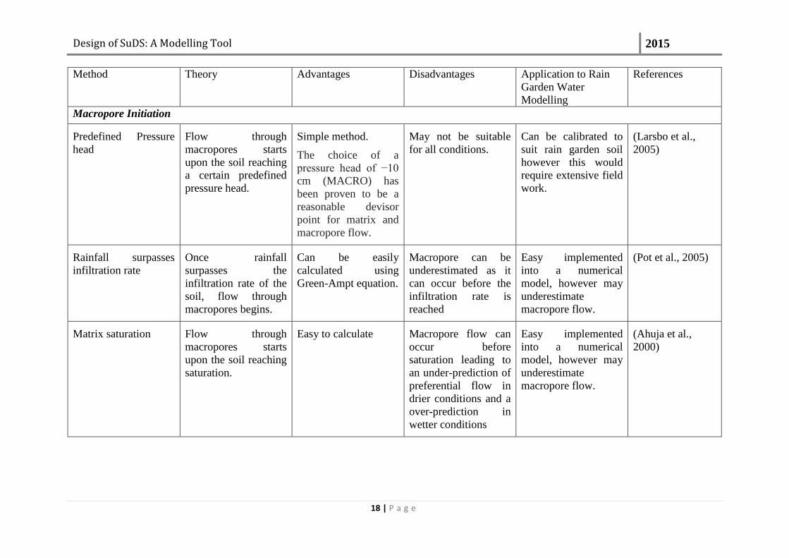
Design of SuDS: A Modelling Tool 2015
18 | P a g e
Method Theory Advantages Disadvantages Application to Rain
Garden Water
Modelling
References
Macropore Initiation
Predefined Pressure
head
Flow through
macropores starts
upon the soil reaching
a certain predefined
pressure head.
Simple method.
The choice of a
pressure head of −10
cm (MACRO) has
been proven to be a
reasonable devisor
point for matrix and
macropore flow.
May not be suitable
for all conditions.
Can be calibrated to
suit rain garden soil
however this would
require extensive field
work.
(Larsbo et al.,
2005)
Rainfall surpasses
infiltration rate
Once rainfall
surpasses the
infiltration rate of the
soil, flow through
macropores begins.
Can be easily
calculated using
Green-Ampt equation.
Macropore can be
underestimated as it
can occur before the
infiltration rate is
reached
Easy implemented
into a numerical
model, however may
underestimate
macropore flow.
(Pot et al., 2005)
Matrix saturation Flow through
macropores starts
upon the soil reaching
saturation.
Easy to calculate Macropore flow can
occur before
saturation leading to
an under-prediction of
preferential flow in
drier conditions and a
over-prediction in
wetter conditions
Easy implemented
into a numerical
model, however may
underestimate
macropore flow.
(Ahuja et al.,
2000)

Design of SuDS: A Modelling Tool 2015
19 | P a g e
Method Theory Advantages Disadvantages Application to Rain
Garden Water
Modelling
References
Water Transfer
Mass driven-effective
water content
The water transfer
between matrix and
macropores and vice-
versa is a function of
the soil moisture
content in both flow
regimes.
Simple to use
Doesn’t require many
parameters.
Has only been used in
conjunction with a ‘cut
and join’ approach to
hydraulic functions
and may need
adaptation to be used
with other techniques.
Accurate in soils
similar to SuDS but
never previously been
applied to rain
gardens.
(Larsbo et al.,
2005)
Mass driven-pressure
head
The water transfer
between matrix and
macropores and vice-
versa is a function of
the pressure head in
both flow regimes.
Accurate. Complex and may be
fundamentally
numerically unstable
as the product of two
highly non-linear
terms needs to be
calculated.
Accurate in soils
similar to SuDS but
never previously been
applied to rain
gardens.
(Simunek et al.,
2009)
Green-Ampt Water transfer is
described using the
Green-Ampt equation
for cylindrical
pores.
Simple to use term. Requires geometric
parameters of the
macropores
Generally assumes
water transfer from
macropores to matrix
only.
Accurate in soils
similar to SuDS but
never previously been
applied to rain
gardens.
(Ahuja et al.,
2000)

Design of SuDS: A Modelling Tool 2015
20 | P a g e
A summary of all relevant hydrological computer models is given in Appendix A.
3.4.2 Evapotranspiration
Evapotranspiration is an important factor of modelling water movement in soils. It refers to the
sum of evaporation and transpiration of the plants present in the rain garden. In previous
literature, energy-balance approaches have proven to be the most popular method of calculating
evapotranspiration, specifically the Penman equation and its revisions (Dingman, 1994;
Campbell & Norman, 1998). The Penman-Monteith equation has been shown to be reliable in
various situations and climatic conditions; this is due to incorporation of various calibrated
parameters such as leaf area index, vegetation height and canopy resistance (Allen, et al., 1989;
Ventura et al., 1999).
However, there are continuing problems applying energy-balance equations such as the above
as they require a significant amount of data which is difficult to obtain, especially wind and
relative humidity. Other simpler methods such as the Priestly-Taylor equation exploit the
intrinsic conservative and seasonal predictability of evaporation (Priestly & Taylor, 1972). The
Priestly-Taylor equation has been shown to give a good estimation of evapotranspiration for
numerous different situations including irrigation and intrinsically dry and wet conditions
(Ding, et al., 2013, Ngongondo, et al., 2013). Fowler (2002) compared monthly average
approaches as well as daily estimates using the Priestly-Taylor equation and it was seen that,
for estimating long-term soil water balance, a monthly average performs as well as a daily
value. It has also been used by RECHARGE to model evapotranspiration in rain gardens.
In this method, the total potential evaporation (Ep) (cm) is given by (Priestly & Taylor, 1972):
Ep =∝Δ
Δ+γ
𝑅𝑛
λ (3.1)
where ∝ (Dimensionless) is the ratio of actual to equilibrium evaporation commonly taken as
1.26, Δ (Dimensionless) is the slope of the saturation vapour pressure curve at air temperature,
Rn (W/m²) is the net radiation, G (W/m²) is the soil heat density, γ is the psychrometric constant
(6.66x10⁻⁴ 1/oC), λ (oC) is the latent heat of vaporization. In some cases a plant canopy can
intercept part of the incoming radiation, in such a situation the total potential evaporation can
be split into the potential soil evaporation Es (cm/s) and the potential plant transpiration Tp
(cm/s). Thus, if the transmissivity coefficient of the plant canopy is denoted by τ
(Dimensionless), the potential soil evaporation and the potential plant transpiration are given
by:

Design of SuDS: A Modelling Tool 2015
21 | P a g e
Es = τ∆
∆+γ
𝑛
λ (3.2)
Tp = (α − τ)Δ
Δ+γ
𝑅𝑛
λ (3.3)
The transmissivity coefficient τ can be approximated by (Campbell & Norman, 1998):
τ = exp(−β. LAI) (3.4)
where β (Dimensionless) is the attenuation coefficient and LAI (Dimensionless) is the leaf area
index.
3.4.3 Conclusions on Water Modelling
As is clear from this section, there are numerous dual-permeability approaches in existence,
however they do not currently meet the needs required to model flow in a rain garden with a
simple layered profile and coupled upper boundary conditions (for ponded and non-ponded
conditions). Thus, a new model must be created, the previous models used for groundwater
recharge estimations for rain gardens are not sufficient as they do not include macropore region
flow modelling which has been shown to have an impact on heavy metal retention. The
information gathered above with regards to current methods for prediction of water flow in
both regions, initiation of macropore flow and interaction between the matrix and macropore
regions will be used to develop the water modelling section of the pollutant retention model.
The steps taken to design such a model will be fully detailed in Chapter 4.
The next stage of the literature review is to examine current methods of modelling heavy metal
transport and capture in order to facilitate the design of the pollutant retention segment of the
computer model.
3.5 Heavy Metal Adsorption
As stated previously (Table 3.1) adsorption is the principal mechanism by which pollutants are
removed from runoff in a sustainable drainage system such as a rain garden. The adsorption
process is a surface phenomenon in which a multi-component fluid (gas or liquid) mixture is
drawn towards the surface of a solid adsorbent and forms an attachment through physical or
chemical bonds (Foo & Hameed, 2010).
The overall strength with which metals are retained in soils is dependent on several factors
(Alloway, 2013)
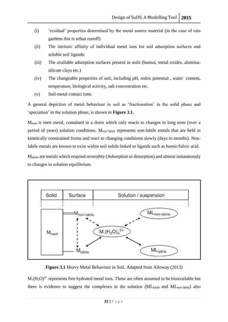
Design of SuDS: A Modelling Tool 2015
22 | P a g e
(i) ‘residual’ properties determined by the metal source material (in the case of rain
gardens this is urban runoff)
(ii) The intrinsic affinity of individual metal ions for soil adsorption surfaces and
soluble soil ligands:
(iii) The available adsorption surfaces present in soils (humus, metal oxides, alumina-
silicate clays etc.)
(iv) The changeable properties of soil, including pH, redox potential , water content,
temperature, biological activity, salt concentration etc.
(v) Soil-metal contact time.
A general depiction of metal behaviour in soil as ‘fractionation’ in the solid phase and
‘speciation’ in the solution phase, is shown in Figure 3.1.
Minert is inert metal, contained in a dorm which only reacts to changes in long term (over a
period of years) solution conditions. Mnon-labile represents non-labile metals that are held in
kinetically constrained forms and react to changing conditions slowly (days to months). Non-
labile metals are known to exist within soil solids linked to ligands such as humic/fulvic acid.
Mlabile are metals which respond reversibly (Adsorption or desorption) and almost instanteously
to changes in solution equilibrium.
Figure 3.1 Heavy Metal Behaviour in Soil. Adapted from Alloway (2013)
M.(H2O)2+ represents free hydrated metal ions. These are often assumed to be bioavailable but
there is evidence to suggest the complexes in the solution (MLlabile and MLnon-labile) also

Design of SuDS: A Modelling Tool 2015
23 | P a g e
contribute to bioavailability. All forms of metal contained in solutions or suspended is subject
to transportation in water.
Examples of the above surface and solid metal states with specific reference to rain garden
devices is shown in Table 3.3.
Table 3.3 Surface and Solid Metal States in a Rain Garden
Metal State Example
Minert Secondary (e.g., phosphate, carbonate) metal compounds solubilised by slow
oxidation reactions or dissolution over extended periods
Mnon-labile Surface adsorbed metals held strongly on mineral or organic surfaces
Mlabile Some specifically-adsorbed metal ions on Fe/Mn/Al hydrous oxide surfaces
and humus.
By far the most common types of metals contained in urban runoff are Cu, Pb and Zn, these
will be examined in greater detail in the subsequent section.
3.5.1 Cu
Traffic is responsible for a large amount of Cu present in urban runoff and thus input into rain
garden soil. This is attributed to both rail transport (corrosion of overhead wires) and road
transport (brake and tire wear). Additional Cu sources include external building applications
such as Cu roofs. This can result in maximum Cu concentrations of 140 μg/L in urban runoff
(Gobel et al. 2007).
The most common forms of Cu are cuprous (Cu1+) and cupric (Cu2+). Cuprous Cu is unstable
in urban runoff transferred to rain garden soil and soluble Cu1+ compounds form Cu2+ ions or
compounds and/or Cu(s) as a precipitate. When Cu2+ is introduced into the soil, the cupric ion
binds to inorganic matter. The Cu2+ ion forms stable complexes with –NH2, -SH, and, to a
lesser extent, -OH groups in these organic acids. It has been found in speciation studies that in
excess of 98% of the soluble Cu in soil was bound to organic ligands. Results from long-term
studies indicate that Cu moves from easily extracted pools to more strongly bound forms. This
results in limited desorption of Cu from soil. The proportion of Cu2+ in a solution decreases
with increasing pH. In rain gardens and native European soils the pH ranges from pH 3.4-6.8,

Design of SuDS: A Modelling Tool 2015
24 | P a g e
resulting in 73% to 99.96% of Cu being complexed. Excess Cu in the soil can result in
detrimental impacts to plants, invertebrates and microorganisms. The table below shows the
Cu threshold concentrations for plants and invertebrates.
Table 3.4 Cu Threshold Concentrations for Plants and Invertebrates (Alloway, 2013)
Range (mg Cu Kg-1 soil)
Monocotyledon Plants
e.g palms, grasses, corn, lillies, tulips, daffodils
18-537
Dicotyledon Plants
e.g. roses, oaks, maples and sycamore
36-698
Arthropods
e.g. insects, arachnids, crustaceans
31-1460
Annelida and Nematoda e.g worms 150-500
The wide range of toxicity values is attributed to the discrepancies between spiked tests and
long term studies. For example it has been found that soils which have been inundated with Cu
to test the detrimental effects on plants and invertebrates show larger toxicity than those in field
tests which have been exposed to a gradual accumulation of Cu over many years. The latter
scenario would be most applicable to rain garden. European risk assessments of Cu
recommend a PNEC (Predicted No Effect Concentration) of between 10 and 200 mg kg-1.
Clean-up standards for Cu soils are generally higher than this ecological standard and the clean-
up limit for Cu in residential soils and industrial soils are 100 mg kg-1 and 200 mg kg-1
respectively in Sweden (the U.K has no guidelines on Cu concentrations in soils) (Provoost et
al., 2006).
3.5.2 Pb
In the past the vast majority of Pb in urban runoff was attributed to leaded petrol since its’
elimination, Pb concentration has decreased. It is still present in smaller concentrations
however which is attributed to Pb roofs, tyre and brake pad abrasion with a maximum
concentration of 575 μg/L in urban runoff (Gobel et al. 2007).

Design of SuDS: A Modelling Tool 2015
25 | P a g e
Dissolved Pb exists in several states in a soil solution: organic complexes, inorganic ion pair
and free Pb2+. It was found by Sauve et al. (1997) that the free Pb2+ activity in soils can be
predicted accurately solely as a function of pH and is not dependent on other characteristics
such organic matter content. Pb in soils generally exists in the Pb+2 oxidation state, but is less
soluble with increasing pH in the soil solution due to sorption onto organic matter. Pb has been
found to be strongly adsorbed onto humic matter, clay minerals depending on soil composition.
It exhibits stronger retention in soil than other heavy metals such as Cu and Zn. This is
supported by previous experimental findings relating to rain gardens which will be discussed
later. Despite this sorption in longer term studies Pb leaching through soils has been observed.
This leaching has been attributed to the release of organic matter from the soil which contained
Pb. This will not be the case in rain garden soil as organic matter will not leave the device.
High levels of Pb in urban soils have been identified as a concern as soil is seen as an important
pathway of human lead exposure, in particular to children engaged in hand-to-mouth and pica
behaviour. As rain gardens may be located in residential and school areas these findings are of
concern when designing these devices.
In the U.K the regulatory limit of Pb in soils is 450 and 750 mg Kg-1 for residential and
industrial landuse respectively. If these levels are exceeded in a rain garden as predicted by Li
and Davis, several options are available for remediation including removal and amendment
with phosphate.
3.5.3 Zn
The presence of Zn in urban runoff is attributed primarily to tyre debris and Zn coated roofs,
this can result in concentrations of up to 2000 μg/L (Gobel et al. 2007).
Similar to Pb and Cu, Zn exists as the Zn2+ oxidation state in soils. This concentration is
regulated by sorption and mineral dissolution reactions where sorption is the dominant reaction.
Zn can experience strong sorption onto numerous soil components such as organic matter and
on Fe and Mn oxides. Alternatively weaker reversible reactions can occur by adsorption
through ion exchange on clay mineral surfaces. Soil acidity also decreases the solubility of Zn
in a similar fashion to Pb with the free ion fraction decreasing with increasing pH.
When Zn is initially input into soil, there is an almost immediate reaction in which Zn adsorbs
onto the solid phase. This reaction is rapid, following this slower reactions occur that form

Design of SuDS: A Modelling Tool 2015
26 | P a g e
bonds between the Zn and soil from which desorption is slow. This limits the release of Zn
from the soil but increases toxicity.
Although Zn is an essential nutrient for plants, excess content in soil may result in plant
toxicity. Typically there is a 10% reduction in plant yield at soil concentrations of 100 mg/Kg.
This is due to increased plant Zn concentrations causing reduced root growth or stunted shoot
growth. In the U.K the regulatory limit of Zn in soils is 500 mg/Kg for industrial land-use, no
current limits are in existence for residential areas however in Sweden it is 350 mg/Kg (Suave
et al., 1997).
3.5.4 Heavy Metal Fractions
Depending on soil properties and the heavy metals present, adsorption of the metal is associated
with different chemical fractions. The chemical fraction of a metal is the determining factor for
environmental mobility, bioavailability and the likelihood of desorption. The sequential
extraction method developed by Tessier (1979) provides a useful analytical method for
partioning of particulate trace metals into five geochemical phases:
Fraction 1. Exchangeable
The metals in this fraction are highly bioavailable and show mobility relative to their
environment and are potentially available to plants. Changes in ionic composition could result
in desorption of metals in this fraction.
Fraction 2. Bound to Carbonates
Metals in this fraction are also bioavailable and susceptible to changes in pH.
Fraction 3. Bound to Iron and Manganese Oxides
Iron and manganese oxides exist in soils as the adhesive between particles or as a particle
coating.
Fraction 4. Bound to Organic Matter
It has been found that metals can bind to numerous forms of organic matter such as living
organisms and coatings on mineral particles. However under oxidising conditions in natural
waters, organic matter can be degraded resulting in the release of soluble metal.
Fraction 5. Residual
The metals held in this fraction are generally found in the crystal structure of primary and
secondary minerals. These metals are not expected to be released into the environment over a
reasonable time span under conditions found in nature.

Design of SuDS: A Modelling Tool 2015
27 | P a g e
Numerous studies have quantified the metal fractions in both rain garden and road side soils
using Tessier’s (1979) method. It has been found that metal fractions in F1 are generally low,
the bulk of accumulation occurring in environmentally inaccessible fractions (F3 through F5)
therefore metals captured in rain garden media are expected to remain largely immobile
(Sansalone & Buchberger,1997; Wilcke, et al., 1998; Li, et al., 2001; Li & Davis, 2008).
There has been much criticism of Tessier’s and other sequential extraction methods due to the
non-selectivity of reagents used in testing which may alter the characteristics of sediments
tested. This usually results in metals collected for fractions 1-3 were underestimated and
fractions 4-5 overestimated (Zimmerman & Weindorf, 2010). This is turn underestimates the
possible release of metals from the soils.
Therefore, traditional chemical testing such as Tessier’s (1979) method cannot ensure that all
toxic chemicals of importance are identified and measured in the sediment of interest; nor can
they be used to estimate synergistic effects among compounds in a solution (Wang, et al.,
1998). Biological testing has, therefore, become an important tool in enhancing the traditional
environmental monitoring programmes based on chemical tests to characterise complex
chemical mixtures in sediments and water. Biological toxicity testing is based on exposing
organisms to all the bioavailable chemicals in a test sample and then noting the changes in
biological activity.
In conclusion, although recent research into heavy metal fractions in rain gardens and other
SuDS have shown that heavy metals are strongly retained in the soil, these findings are limited
by the analysis techniques used and should be treated with caution. In future it is recommended
that more accurate methods which reflect natural soil conditions be used such as biological
testing.
As stated in Section 1.3, the main aim of this thesis is to predict the adsorption of heavy metals
in rain garden soil. Over the years, many isotherm models (Langmuir, Freundlich, Brunauer-
Emmett-Teller, Sips etc.) have been developed to predict adsorption. An adsorption isotherm
is a curve representing the process controlling the retention or movement of a substance from
the aqueous porous media to a solid-phase at a constant temperature and pH (Ho, et al., 2001).

Design of SuDS: A Modelling Tool 2015
28 | P a g e
3.5.5 Sorption Experiments
Several studies have been completed into the suitability of selected isotherms for modelling
the adsorption of heavy metals onto various absorbents and in rain garden systems (Davis et
al., 2001, Li & Davis, 2008).
The accuracy of a great range of isotherms was examined by Ho et al. (2001). Here the sorption
of the metals Cu and Pb onto peat was examined using sorption experiments and the results
compared with those calculated using the Langmuir, Freundlich, Redlich-Peterson, Toth,
Temkin, Dubinin-Radushkevich and Sips (combined Langmuir-Freundlich) isotherm models.
It was found that in all cases the three parameter Sips isotherm equation offered the best fit to
the equilibrium data.
Jang et al. (2005) also examined heavy metal removal (Cu, Pb, Zn) from urban storm water by
various types of mulch using sorption experiments. The results from these experiments were
then compared to the predictions given by the Langmuir and Freundlich isotherms in order to
ascertain the better predictor of adsorption. It was found that the Langmuir isotherm was more
accurate in all cases with an R2 (correlation coefficient) value of between 0.997 and 0.999 as
opposed to values as low as 0.848 for the Freundlich model.
Li and Davis (2008) modelled the absorption of Cu, Pb and Zn in a rain garden using a linear
isotherm. They compared their results to an 85-90cm core sample from a 4.5 year old rain
garden system with media consisting of 50% sand, 30% top soil and 20% mulch. Their model
not only took into account the absorption of the metals to the media but also to total suspended
solids (TSS) in the urban runoff. This was accomplished by incorporating the average input
TSS and a filter parameter into the calculation of metal distribution coefficients which were
used to determine the quantity of contaminant retained. Their results indicated a successful
prediction of heavy metal retention especially in the cases of Pb and Zn with Cu however, the
retention was not modelled as accurately, possibly owing to its weaker association with the
soil, desorption or incorrect linear assumptions. Li and Davis (2008) concede that if a more
accurate numerical model is required, non-steady state and nonlinear isotherms would be
needed but this would greatly increase model complexity and input data requirements.
Genc-Fuhrman et al. (2007) examined the potential use of alumina, activated bauxsol-coated
sand, bauxsol-coated sand, fly ash, granulated activated carbon (GAC), granulated ferric
hydroxide, iron oxide-coated sand (IOCS), natural zeolite, sand and spinel as sorbents for

Design of SuDS: A Modelling Tool 2015
29 | P a g e
removing heavy metals from storm water; in this case the relevant metals tested were Cd, Cu
and Zn. The results of their experiments were then compared to the predictions of the
Freundlich isotherm which was deemed to give a better fit than the Langmuir model. For the
adsorbents, fly ash, spinel and bauxsol-coated sand, low values for R2 were obtained (as low
as 0.2), this was blamed on other removal mechanisms which the Freundlich isotherm was
unable to predict. Low R2 values for substances such as sand can also be caused by leaching of
some metals from the sorbents and oversaturated conditions which results in precipitation
becoming the leading removal mechanism over sorption. The results from other sorption
experiments are shown in Table 3.5.

Design of SuDS: A Modelling Tool 2015
30 | P a g e
Table 3.5 Results of a Variety of Heavy Metal Sorption Experiments
Metals
Tested
Adsorbent Isotherms Verification
Method
Findings Source
Cadmium Pine bark Freundlich Visual Good Correlation (Al-Asheh &
Duvnjak., 1997)
Copper
Lead
Tea waste
GAC
Freundlich
Langmuir
Correlation
Coefficient
Both Isotherms performed well with R2> 0.95 for both
metals
(Amarasinghe &
Williams, 2007)
Cadmium
Copper
Lead
Red Mud
Fly Ash
Langmuir Correlation
Coefficient
Fly Ash exhibited the greater amount of retention.
The Langmuir isotherm performed well for both
adsorbents and for all metals with R2>0.95 in every case.
(Apak, et al.,
1998)
Cadmium Juniper Fiber Langmuir
Freundlich
Correlation
Coefficient
The Langmuir isotherm exhibited a fractional advantage
over the Freundlich isotherm with an R2 value of 0.997 as
opposed to 0.938.
(Min, et al.,
2004)
Copper
Zinc
Clay Langmuir Correlation
Coefficient
Langmuir Isotherm performed well with an R2 value of
0.99 for both metals
(Vengris, et al.,
2001)
Copper
Lead
Zinc
Zeolite Sips, Redlich-
Peterson, Toth,
Dubinin-
Radushkevich,
Linewer-Burk
Correlation
Coefficient
All the isotherms showed good accuracy with R2>0.92 in
all cases. However Sips was to some extent the best fitting
curve.
(Peric, et al.,
2004)
Cadmium
Copper
Activated
carbon,
kaolin,
bentonite,
diatomite and
waste
materials
such as
compost
Langmuir
Freundlich
Correlation
Coefficient
For copper the Langmuir isotherm was more accurate on
all the absorbents save for compost where the Freundlich
model proved better with a R2 value of 0.95 as opposed
to 0.94.
For cadmium, the Langmuir model suited active carbon,
compost and cellulose pulp waste better whereas the
Freundlich equation gave better results for kaolin,
bentonite and diatomite.
(Ulmanu, et al.,
2003)

Design of SuDS: A Modelling Tool 2015
31 | P a g e
From the findings of previous experiments, it is clear that four principal isotherms are apparent
as the most common methods of heavy metal prediction; the linear, Langmuir, Freundlich and
Sips isotherms. These will be examined in the following sections.
3.5.6 Linear Isotherm
The linear isotherm is the simplest in isotherm theory and is essentially an interpretation of
Henry’s law of gases (Kulprathipanja, 2010). It assumes that the media-sorbed pollutant
concentration (Cs) (mg/kg) is directly proportional to the dissolved pollutant concentration (C)
(mg/L) (Kulprathipanja, 2010):
𝐶𝑠 = 𝐾𝑑𝐶 (3.5)
where Kd is the linear distribution coefficient (L/kg). The distribution coefficient is one of the
determining factors of pollutant retention; it is a measure of the ability of a media such as soil
to retain contaminants and also the affinity of the metal to sorb to the specific media. It varies
between both media and metals with metals such as Pb and Zn having higher distribution
coefficients in soils than Cu (Li & Davis, 2008). If the concentrations are low it has been found
that this isotherm can quite accurately describe adsorption (Kulprathipanja, 2010). This
supports its use as a method for the prediction of pollutant retention in rain gardens as the levels
of heavy metal concentrations are typically low (Davis, et al., 2001). As opposed to other more
complex equations, only one parameter is needed, Kd which gives it a decided advantage when
information about soil is not readily available.
It has been found from experiments that the capacity for a media to retain heavy metals varies
widely (Davis, et al., 2001; Morera, et al., 2001; Li & Davis, 2008). It depends not only on the
constituents of the soil such as organic matter content but also on factors such as pH and
adsorption preferences which will be discussed later (Section 3.5.10). The linear isotherms
main advantage is its simplicity and the relative ease by which its parameters can be obtained
however this results in a lack of accuracy as experienced by Li and Davis (2008). Increasing
accuracy can be obtained by exploiting more complex isotherms.
3.5.7 Langmuir Isotherm model
The Langmuir isotherm has conventionally been used to assess and compare the capacities of
various bio-sorbents. At low pollutant input concentrations, it essentially reduces to a linear
isotherm as detailed above and obeys Henry’s law. At higher input concentrations it assumes
monolayer adsorption, meaning the adsorbed layer is one molecule thick and that adsorption is

Design of SuDS: A Modelling Tool 2015
32 | P a g e
only present at a fixed number of definite sites that are identical and equivalent, with no lateral
interaction and steric hindrance between the adsorbed molecules. This signifies that an
equilibrium saturation point can be reached whereby once a molecule occupies a site no further
adsorption occurs (Foo & Hameed, 2010). In a device such as a rain garden, this can lead to a
complete saturation of the soil media with heavy metals resulting in the input concentration
travelling through the system without being adsorbed. This is a situation which requires further
examination and design, and will be discussed later. The nonlinear form of the Langmuir
isotherm can be represented as follows (Foo & Hameed, 2010):
𝐶𝑠 =𝐾𝐿𝑆𝑚𝑎𝑥𝐶
1+𝐾𝐿𝐶 (3.6)
where KL (L/kg) is the Langmuir isotherm coefficient and Smax (mg/Kg) is the total
concentration of sorption sites available.
Numerous studies have examined the Langmuir coefficients for various absorbents (Ulmanu,
et al., 2003; Seelsaen, et al., 2006; Amarasinghe & Williams., 2007; Nwachukwu & Pullford,
2008). It was found that the Langmuir provided an accurate prediction for a wide range of
media, pH values and metals with R2>0.92 in all cases, however a number of disadvtanges
were identified.
It does not account for the surface roughness of particles in the adsorbate (Foo & Hameed,
2010). Rough surfaces can have multiple sites for adsorption which disagrees with the
Langmuirs monolayer theory. Although in rain garden, soils with low particle roughness are
generally used such as mulch or peat, the use of sand to reduce nutrients is becoming
increasingly common (Hsieh & Davis, 2005). Thus the Langmuir isotherm may not always be
appropriate, the Freundlich isotherm however models multilayer absorption and will be
examined next.
3.5.8 Freundlich Isotherm
The Freundlich isotherm is the earliest known sorption isotherm equation. It is an empirical
model which can predict non-ideal sorption (this is non-uniform sorption with stronger binding
sites being occupied first) as well as multilayer sorption (Ho, et al., 2002). In recent years the
Freundlich isotherm has been extensively applied in heterogeneous systems and can be
represented as (Ho, et al., 2002):
𝐶𝑠 = 𝐾𝐹𝐶𝑎𝐹 (3.7)

Design of SuDS: A Modelling Tool 2015
33 | P a g e
where KF (L/kg) is the Freundlich constant and aF (Dimensionless) is the Freundlich exponent.
This equation has been criticised in the past few years because it lacks a fundamental
theromodynamic basis as it does not reduce to Henry’s law at low concentrations (Ho, et al.,
2002). This could cause a problem as typically heavy metal concentrations in storm water are
low, however the Freundlich isotherm has shown good results when previously tested at these
low levels (Genc-Fuhrman, et al., 2007).
3.5.9 Sips Isotherm
The Sips isotherm model is a three parameter isotherm and is a combined form of the Langmuir
and Freundlich expressions derived for modelling hetrogeneous adsorption systems. This
combination of isotherms reduces the inaccuracies experienced when applying them
individually. At low input concentrations, it reduces to a Freundlich isotherm; while at high
concentrations, it predicts the monolayer adsorption typical of the Langmuir isotherm. It can
be represented as (Ho, et al., 2001):
𝐶𝑠 =𝐾𝐿𝐹𝐶
𝑛𝐿𝐹
1+(𝑎𝐿𝐹𝐶)𝑛𝐿𝐹
(3.8)
where KLF (L/kg) is the Langmuir-Freundlich isotherm constant, nLF (Dimensionless) and aLF
(Dimensionless) are Langmuir-Freundlich isotherm exponents. The Sips isotherm however
does not obey Henry’s law at low concentrations (as it reduces to the Freundlich isotherm)
typical of the heavy metals in runoff, thus it has no thermodynamic grounding. It also has three
parameters which need estimation and has not commonly been used in the prediction of heavy
metal retention when compared to the other isotherms examined so experimental values of
these parameters are lacking.
3.5.10 Other Impacting Factors on Heavy Metal Retention
Co-ion effect and Competitive Adsorption
Storm water runoff generally contains a combination of several metals, this results in a co-ion
effect which can have a crucial role in sorption. This effect is produced by the existence of
different ions in runoff such as Cu2+, Pb2+, Zn2+ which compete with one another for sorption
sites. Several experiments have examined this phenomenon and it has been found that in mixed
metal solutions, the adsorption capabilities of a particular metal ion has been lessened by the
presence of other metals which results in a decrease in removal efficiency (Jang, et al., 2005).

Design of SuDS: A Modelling Tool 2015
34 | P a g e
For example, the adsorption of Cd is strongly affected by the occurrence of competing cations
such as divalent Ca and Zn, which compete with Cd for sorption sites in the soil (Bradl, 2004).
In the case of Jang et al. (2005), the order of adsorption was similar to the results obtained for
single component testing of Pb>Cu>Zn. This corresponds to the findings of Bradl (2004) for
peat and Gomes et al. (2001) for subsoil. This finding is reflected in the majority of the cases
discussed, the main exceptions to this being the linear isotherm cases of Davis et al. (2001) and
Li and Davis (2008) who found that for rain garden soil specifically the order of adsorption
followed Pb>Zn>Cu. These experiments, however did not reach complete breakthrough.
Heavy metal breakthrough is defined as the point at which inflow metal concentration is equal
to outflow concentration. Thus, these experiments could have reached the same sorption
preference found by the experiments of Gomes et al. (2001), Brandl (2004) and Jang et al.
(2005) if a longer experimental period had been observed. In the case of Li and Davis (2008)
additional factors could have played a part, such as soil composition and the presence of other
metal ions which inhibited the adsorption of Cu.
Effects of pH
Soil pH is a crucial parameter which affects metal-solution and soil-surface chemistry and
adsorption. Usually, heavy metal adsorption is small at low pH values as the quantity of
negatively charged surface sites is low and increases with increased pH. Adsorption then
increases at intermediate pH values from near zero to near complete adsorption over a small
pH range; this pH range is known as the pH-adsorption edge. This result has been exhibited
well by the findings of Bradl (2004) where the absorption of Cd, Cu and Zn onto sediment
increases from near zero at pH 4 to near complete at pH 7. This conclusion is confirmed by the
findings of Christensen et al. (1996) who examined the retention of these heavy metals in sandy
aquifer material and found that the adsorption capacity of the soil greatly diminished with
decreasing pH.
As pH has such an impact on adsorption, studies have attempted to quantify its effects using
an extension of the Freundlich isotherm. Van der Zee and van Riemsdijk (1987) suggested the
inclusion of soil pH as H+ and organic carbon in the Freundlich isotherm
Van der Zee and van Riemsdijk (1987) found their approach accurately reflects the molecular
impact pH has on heavy metal retention and is a useful as a tool for assessing metal capture
across the pH range from extremely acidic to basic soils. However, as well as increasing
accuracy, their approach also requires the quantification of a number of complex parameters.

Design of SuDS: A Modelling Tool 2015
35 | P a g e
As a rain garden is an artificial creation it is possible to use soils in the optimum pH range,
which can then be maintained. Of course this approach is not appropriate in areas which are
prone to acid rain but these cases can be assessed separately.
Organic Matter Content and Chemical Composition of Soil.
It has been shown that both organic matter content and the chemical composition of soil can
greatly affect its ability to retain metals. Hsieh and Davis (2005) examined the retention of Pb
for a variety of different media compositions. It was found that levels of organic matter were
seen to increase the retention of Pb. However when mulch (29.8% organic matter) was the
main component of the substrate, a drop in retention was seen, this can be explained by the
high number of larger coarse particles in this material, that leads to voids and preferential
channels which can inhibit metal capture. Cu also has an affinity to organic matter by its
preference for binding to organic ligands. The addition of organic carbon to rain garden column
experiments performed by Blecken et al. (2009) also resulted in larger removal of Cu further
proving the influence of organic matter on the adsorption of Cu. Further sinks for Cu include
iron and maganese oxides and sulphides (Fraction 4). Zn is less affected by organic matter but
is readily sorbed to minerals present in soils such as clays.
3.5.11 Conclusions
In conclusion, the isotherms which will have proved the most accurate and beneficial in
previous research are the linear, Langmuir and Freundlich isotherms. Each isotherm provides
certain advantages, the simplicity of the linear isotherm provides a good starting point for the
pollutant retention model and proves useful when information regarding the soil type is used
and it is also to date the only model which has been applied to existing SuDS. The Langmuir
isotherm is a more complex and more accurate equation which has been used effectively on
numerous soils however it is not applicable to all soil types such as those with high surface
roughness. The Freundlich isotherm is again complex but can be used in situations where the
Langmuir isotherm is inappropriate such as for coarse grained soils. The Sips isotherm was
also proven to be applicable but it introduces additional complexities in the form of a third
unknown variable (Ho, et al., 2001)
Section 3.5.10 showed that caution must be taken when selecting adsorption distribution
coefficients so as to account for both the co-ion effect and also the degree to which factors such
as chemical composition of the soil and the organic matter content will affect heavy metal

Design of SuDS: A Modelling Tool 2015
36 | P a g e
retention. The value of pH is also important as it has a direct impact on the capacity of the soil
to adsorb heavy metals.
These isotherms cannot be used solely to model the retention of pollutants in a rain garden as
they simply predict the mass of pollutant removal per mass of media. The retention of metals
in a SuDS such as a rain garden is far more complex and dependent on other factors such time,
depth and the volume of input; this will be examined in the next section.
3.6 Heavy Metal Transport and Retention
3.6.1 Transport and Retention in the Matrix Region
The principle mechanisms which control solute transport in soil have been identified as
advection and hydrodynamic dispersion (Freeze & Cherry, 1979). Advection is related to
average water flux or velocity. The hydrodynamic dispersion is analogous to a diffusion-like
process which is assumed to be the result of Brownian motion of solute particles. Brownian
motion is the presumption that particles suspended in a fluid move in a random pattern. The
dispersion component also adheres to Fick’s law which states that the flux moves from regions
of high concentration to regions of low concentration with a magnitude proportional to the
concentration gradient. These assumptions lead to the parabolic advection-dispersion equation
(ADE):
𝜕𝐶
𝜕𝑡= 𝐷
𝜕2𝐶
𝜕𝑧2− 𝑣
𝜕𝐶
𝜕𝑧 (3.9)
where C (mg/L) is the solute concentration, D (cm2/s) is the dispersion coefficient, v (cm/s) is
the average pore water velocity, z (cm) is the vertical distance travelled and t (s) is the time.
This is the mass conservation equation for transport of nonreactive solute through
homogeneous porous media. In order for the dispersion coefficient to equal diffusion, a solute
moving by advection in the direction of the mean transport at a rate different from 𝑣 must have
time to mix with the wetted soil. If this is not the case, as with larger scales (regional) and
deeper soils, the ADE cannot describe the transport with a constant D, as increased variability
in the constituency of soils enhance solute dispersion (Section 3.6.1.2). The ADE is the most
popular method of solute modelling and has been used by numerous hydrological models
including MACRO and HYDRUS albeit in different forms. For example the equation used by
MACRO is shown below (Larsbo & Jarvis, 2003):

Design of SuDS: A Modelling Tool 2015
37 | P a g e
𝜕(𝐶𝜃)
𝜕𝑡+𝜕(𝐶)
𝜕𝑡=
𝜕
𝜕𝑧(𝐷𝜃
𝜕𝐶
𝜕𝑧− 𝑞𝐶) − 𝑈 (3.10)
where θ (m3/m3) is the soil moisture content, q (cm/s) is the water flow rate and U (mg/L) is a
sink term for pollutants that represents a variety of diverse processes (i.e. mass exchange
between flow domains, kinetic sorption, solute uptake by crops, biodegradation). The
reliability of the ADE is dependent on the situation to which it is applied. It is most accurate
when used to model movement of bulk solutes over moderate distances (< 3m). At microscopic
scales it is erroneous due to insufficient mixing to validate Fickian assumptions.
It has been found that the ADE does not accurately quantify some key aspects of solute
transport through porous media. For instance, the dispersion coefficient has been found to
increase with soil depth whereas in the ADE is it assumed to be constant. In addition the
fundamental assumption of ADE that particles move by Brownian motion has been found to
be far too restrictive in many cases. In order to address these problems several other equations
have been suggested for modelling solute transport in soil, these are discussed briefly below
(van Dam, et al., 2004).
Stochastic-convective model (SCM)
This hypothesis assumes the soil volume is composed of stream tubes with randomly
distributed travel times (Jury & Scotter, 1994). The values of these travel times are presented
as a probability density function which is assumed to be lognormal. With this transport,
mechanism solutes are assumed never to leave their stream tubes, thus the SCM is only able to
model longitudinal spreading within the entire soil volume. It is simpler to implement than the
ADE, however it is unable to handle non-uniform solute applications. It has been found that
the SCM is adept at modelling regional-scale transport of pollutants from subsurface diffuse
sources, such as pipeline leakage.
Continuous-time random walk (CTRW)
This mechanism models solute transport in terms of the probability of a random displacement
with a random travel time (Berkowitz, et al. 2000). This approach offers numerous benefits
including its ability to model movement which is neither stochastic convective nor advective-
dispersive but some approximation of these. Unfortunately this model is difficult to implement
and requires considerably more parameters than other equations.

Design of SuDS: A Modelling Tool 2015
38 | P a g e
Fractional advective-dispersion equation (FADE)
This approach characterizes the intermediate stages between the SCM and the ADE and
includes the ADE as a special case. Its creation was prompted by the failure of the ADE to
accurately quantify field scale solute leaching (Benson, et al., 2000). This model is physically
based on the Lévy process, this is the assumption that a solute particle does not continuously
move between stream tubes but undergoes advective episodes during which Brownian
dispersive episodes occur intermittently. The main disadvantage of this approach is the
difficulty in solving the multidirectional fractional derivatives of which the equation is
composed.
The advantages and disadvantages of the above methods are shown in Table 3.6.
Table 3.6 Advantages and Disadvantages of Models of Pollutant Transfer Methods
Model Advantages Disadvantage
ADE Popular method
Data sets and parameters widely
available
Well researched
Can be solved analytically and
numerically
Simple underlying mathematics
Not reliable over large travel
distances
Fickian assumptions have
limited physical basis
Inaccurate at larger field and
regional scales
Assumptions relating to the
dispersion constant
inaccurate at large depths
(>3m)
SCM Physically based assumptions
Experimental support
Can accurately quantify field
scale solute transport
Travel time probability
density function requires
calibration
Application to layered soils is
difficult
Solute application must be
uniform
CTRW Generalises solute movement
Can model both Fickian and non
Fickian movement
Limited application to
unsaturated transport

Design of SuDS: A Modelling Tool 2015
39 | P a g e
Requires large number of
measurements
Not well researched
FADE Well established physical and
mathematical basis
More flexible than ADE and
SCM
Complex equation
Not well researched.
3.6.1.1 Advection-Dispersion-Adsorption Equation
Advection-dispersion has been used to succesfully predict the movement of heavy metals
through soils (Chang, et al., 2001; Sun & Davis, 2007; Ogata & Banks, 1964). This can be
solved both numerically and analytically. The analytical solution of the advection diffusion
equation for one-dimensional solute transport in semi-infinite soil columns is described by
Ogata and Banks (1964) as:
𝐶(𝑧, 𝑡) = (𝐶
2) {𝑒𝑟𝑓𝑐 [
(𝑧−𝑣𝑡)
2√𝐷𝑡] + exp (
𝑣𝑧
𝐷) 𝑒𝑟𝑓𝑐 [
(𝑧+𝑣𝑡)
2√𝐷𝑡]} (3.11)
where erfc is the error function.
In order to model retention a retardation factor (R) is incorporated into the ADE (Eq. 3.9). This
factor governs the retention of the pollutants and is dependent on the isotherm being used. The
value of R (kg/ m3) can be calculated as follows (Ho, et al., 2001):
𝑅 = 1 +𝜌
𝜃
𝜕𝐶𝑠
𝜕𝐶 (3.12)
where 𝜌 (kg/ m3) is the bulk mass density. The retardation factor was developed by Hashimoto
et al. (1964) to enable the prediction of solute dispersive transport through columns.
The combination of the ADE a retardation factor results in the advection-dispersion-adsorption:
𝑅𝜕𝐶
𝜕𝑡+ 𝑣
𝜕𝐶
𝜕𝑧− 𝐷
𝜕2𝐶
𝜕𝑧= 0 (3.13)
Again as above this equation can be solved numerically or analytically (Ogata & Banks, 1964):
𝐶(𝑧, 𝑡) = (𝐶
2) {𝑒𝑟𝑓𝑐 [
(𝑅𝑧−𝑣𝑡)
2√𝑅𝐷𝑡] + exp (
𝑣𝑧
𝐷) 𝑒𝑟𝑓𝑐 [
(𝑅𝑧+𝑣𝑡)
2√𝑅𝐷𝑡]} (3.14)
The use of these retardation coefficients allows for the prediction of retention as a function of
both the depth of the system (which facilitates examinations regarding the depth at which
polllutants reach in the rain garden) and the time (the pollutant values in the soil can be assessed

Design of SuDS: A Modelling Tool 2015
40 | P a g e
in years allowing for life cycle and remedial work evaluations to be made). For example as
detailed in Section 3.5 Pb has found to exceed soil concentration safety limits in the upper
layers of rain garden.
3.6.1.2 Dispersion
Dispersion performs an important role in the transport of contaminants through porous media.
It takes place as a function of two separate processes: (i) molecular diffusion (ee) (cm2/s), which
is due to Brownian motion and (ii) mechanical dispersion (Dm) (cm2/s) which is produced by
varying velocities and flow path distribution (Gaganis, et al., 2005). Thus the formula for the
dispersion coefficient generally combines both these elements (Matsubayashi, et al., 1997):
𝐷 = 𝐷𝑚 + 𝑒𝑒 (3.15)
It is commonly assumed that mechanical dispersion is proportional to the average linearized
pore water velocity (v) (cm/s) and dispersivity (d) (cm) resulting in the equation (Freeze &
Cherry, 1979):
𝐷𝑚 = 𝑑𝑣 (3.16)
The values of 𝑑 vary and are generally smaller in a laboratory column (0.5 to 2cm) than for
those measured in the field (5 to 20 cm) (Warrick, 2003). It has also been found that this value
is independent of water content and flow rate (Costa & Prunty, 2006). Molecular diffusion can
also be further dissected into a function of tortuosity (τo (Dimensionless)) and binary diffusion
coefficient of the solute in water (D0) (cm2/s):
𝑒𝑒 = 𝜏𝑜𝐷0 (3.17)
𝑒𝑒 generally applies on a microscopic level however when flow rates are small (Jury & Horton,
2004).
It has been noted that for larger water flows the transport process shifts from advection-
dispersion (where α is independent of depth) to a possibly stochastic dispersive process with
dispersivity increasing at greater depths (Costa & Prunty, 2006). This may not be due solely to
higher flow rates but due to the preferential flow caused by them. This was not identified by
the authors but the breakthrough curves they supply for the higher flow rate show anomalies
which could indicate a preferential flow pattern.

Design of SuDS: A Modelling Tool 2015
41 | P a g e
3.6.2 Transport and Retention in the Macropore Region
The advection-dispersion equation can be used to model solute transport in both the matrix and
macropore regions, in some dual permeability models such as RZWQM (Ahuja, et al., 2000)
and IN3M (Weiler, 2005) sorption in the macropore region is often neglected. This assumption
is certainly valid in short periods with high infiltration rates where water transport through
macropores is typified by high velocity and minimal soil-water contact which is necessary for
sorption. However when macropores are saturated, the period of soil-runoff contact is
significantly increased which can lead to sorption in this area (Knechtenhofer, et al., 2003).
3.6.3 Pollutant Transfer
The transfer between matrix and macropore regions is typically represented by a first order
advection-dispersion equation (MACRO, HYDRUS), advection equation (SIMULAT) or in
the case of the RZWQM instant mixing with a boundary matrix layer (Kohne et al., 2009).
Pollutant transport (P) (mg/L) in the direction from macropore (Cma) (mg/L) to matrix (Cmi)
(mg/L) in MACRO is expressed by (Larsbo & Jarvis, 2003):
𝑃 = (𝐺𝑓𝐷𝑒𝜃𝑚𝑎𝑡
𝑑𝑝2 ) (𝐶𝑚𝑎 − 𝐶𝑚𝑖) + 𝐶𝑚𝑎 (3.18)
where Gf (Dimensionless) is a geometry factor, dp (cm) is an effective ‘diffusion’ pathlength,
De (cm2/s) is an effective diffusion coefficient, θmat (m3/m3) is the mobile water content in the
matrix.
3.6.4 Conclusions
The advection-dispersion equation has proven in the past to be an accurate method of predicting
the transport of heavy metals through soil. By combining this equation with various isotherm
retardation factors it is possible to both model the adsorption and transport of heavy metals
simultaneously in soil which reduces computation time and simplifies any proposed model.
Pollutant transport in the macropores is generally modelled using only the advection-dispersion
equation and adsorption in this region is largely neglected unless tackled by a more complex
model such as HYDRUS. Pollutant transfer is often only deemed to occur from the macropore
region (where no sorption occurs) to the matrix region (RZWQM, MACRO). A further point
of consideration is the diverse range of processes represented by U in Eq. 3.10 which may have
to be considered such as mass exchange between flow domains (Section 3.6.3), solute uptake
by crops, biodegradation. The advection-dispersion-retardation equations in the matrix already

Design of SuDS: A Modelling Tool 2015
42 | P a g e
encompasses the kinetic sorption component of the term U. The other components of U are
dealt with as follows:
Solute absorption by plants: As stated above in previous experiments the proportion of heavy
metal uptake by vegetation was found to be minimal in comparison with the percentage which
was retained by the soil via adsorption (Li & Davis, 2008; Blecken, et al., 2009). Thus for this
reason in the initial version of the proposed model, it is assumed to be negligible.
Biodegradation: This is not an issue with heavy metals as unlike carbon-based (organic)
molecules and substances such as pesticides, metals do not degrade. There are two exceptions:
to this mercury and selenium but these are not present in significant concentrations in urban
runoff (Natural Resources Conservation Service, 2000).
Finally, a critical issue in dealing with heavy metals in a rain garden system is the build-up of
heavy metals in the upper layer of soil (Sun & Davis, 2007). This accumulation, especially of
Pb, may lead to metal concentrations in the soil which contravene public health standards; this
can be avoided by monitoring the levels of contamination in the soil and removing the upper
layer when required. The proposed pollutant retention model could help predict approximately
when this removal should occur.
3.7 Summary
This literature review was focused on the optimum method of developing a computer model
for determining the pollutant retention capability of rain gardens. It provides a summary of the
important factors which influence heavy metal capture, the crucial features of dual permeability
modelling and the main issues regarding retention prediction. This information provides the
basis on which the numerical model can be designed which will be discussed in the next
chapter.

Design of SuDS: A Modelling Tool 2015
43 | P a g e
4 MODEL DEVELOPMENT
4.1 Introduction
In this chapter, the development of a heavy metal retention modelling tool is described. As
discussed in the literature review (Section 3.4.1) and Appendix A, several popular
hydrological models (HYDRUS, MACRO, RZWQM etc.) are available for the prediction of
pollutant retention processes in soil. However these models do not meet the specific needs of
predicting heavy metal retention in rain gardens: they are typically complicated to use, do not
model heavy metals and are predominantly designed for agricultural applications. Therefore a
model called HM07 was developed which incorporated all of the important factors relating to
the retention of heavy metals in rain garden soils as identified by the literature review (Chapter
3) and shown in Table 4.1.
Table 4.1 Important Factors in Heavy Metal Retention
Parameter Type Factor
Hydrological Water flow in the matrix and macropore
regions
Initiation of macropore flow
Interaction between regions
Pore water velocity
Dispersion
Soil Heterogeneity of Soil
Organic matter content
Isotherm Distribution Coefficient
Other pH value
The following is a description of the methods used to develop the proposed model, for ease of
explanation it has been divided into both a hydrological and pollutant component.

Design of SuDS: A Modelling Tool 2015
44 | P a g e
4.2 Hydrological Component
In order to model both the matrix and the macropore regions of flow in soil, a dual-permeability
approach was used. This method described the soil as two overlapping pore domains with
water flowing relatively quickly in one region (through macropores and fractures) and slower
in the other region (matrix).
As stated in the literature review (Section 3.4.1) the predominant methods used to calculate
water flow in the matrix zone are: the Green-Ampt equation followed redestribution, the
kinematic wave equation (KWE) and Richards equation, for macropore flow: Richards
equation, KWE, Poeusielles law and the IN3M equation. As the purpose of this thesis was to
develop a simple computer model the Richards equation can be immediately ruled out. It was
also proposed that the same equation by utilised for both matrix and macropore regions, this
left only the KWE as an option. This equation has previously proven successful at modelling
water in the matrix region for situations that would be prevalent in a rain garden system such
as complex surface flux patterns and layered soil (Smith, 1983). It is also accurate at replicating
flow in macropores and has been used by computer models such as MACRO (Larsbo, et al.,
2005).
The difference in the form of the KWE between the two regions lies in the parameters and
boundary conditions used which are discussed below.
4.2.1 Matrix Region
As a rain garden is a layered system, discontinuities arise in the soil moisture content between
layers and it is thus more beneficial to utilise the pressure head (ℎ) (cm) version of the KWE:
𝜕ℎ
𝜕𝑡+
𝜕𝑞
𝜕𝜃
𝜕ℎ
𝜕𝑧= 0 (4.1)
where q (cm/s) is the water flux, θ (m3/m3) is the soil moisture content and t (s) and z (cm) are
the position in time and space respectively.
As discussed in Section 3.4 there are a number of parameters crucial to soil water flow (θ and
unsaturated hydraulic conductivity (K) (cm/s)), these parameters are important both for the
quantification of water behavouir in the rain garden and also to solve Eq 4.1. These were found
using the van-Genuchten-Mualem functions assuming no hysteresis. These equations are as
follows (van Genuchten, 1980):

Design of SuDS: A Modelling Tool 2015
45 | P a g e
𝐾(𝛩) = 𝐾𝑠 𝛩1
2 [1 − (1 − 𝛩1
𝑚)𝑚
]2
(4.2)
𝜃 =𝜃𝑠𝑎𝑡−𝜃𝑟𝑒𝑠
[1+(𝛼𝑣𝑔|ℎ|𝑛𝑣𝑔)]
𝑚𝑣𝑔 + 𝜃𝑟𝑒𝑠 (4.3)
Where 𝛩 (Dimensionless) is the relative water content:
𝛩 = [1
1+(𝛼𝑣𝑔ℎ)𝑛𝑣𝑔]
𝑚𝑣𝑔
(4.4)
where αvg (1/cm) and nvg (Dimensionless) are the van Genuchten parameters and mvg=1-1/nvg,
K (cm/s) is unsaturated hydraulic conductivity, Ks (cm/s) is the saturated hydraulic
conductivity, θsat (m3/m3) and θres (m
3/m3) are the saturated and residual soil moisture contents
respectively.
The Mualem functions were chosen over the alternative Brooks and Corey functions as
although the Brooks and Corey method gives accurate results, a discontinuity is present in the
slope of both the soil water retention curve and the unsaturated conductivity curve near
bubbling pressure (van Genuchten, 1980). This can prevent rapid convergence in numerical
saturated-unsaturated flow problems and consequently could cause difficulties simulating flow
in a rain garden which will undergo numerous wetting and drying events.
4.2.1.1 Numerical Solution of the Matrix KWE and Boundary Conditions
The pressure head form of the KWE (Eq. 4.1) is discretised using a Crank-Nicholson type
finite difference scheme where the weight can be changed from 0.5 (traditional Crank-
Nicholson) to 1.0 (fully implicit).
The upper boundary condition is dependent on the water balance in the rain garden surface
depression which can be expressed as:
𝐴𝑟𝑔𝑑ℎ𝑠
𝑑𝑡= 𝑄𝑟𝑎𝑖𝑛 + 𝑄𝑟𝑢𝑛𝑜𝑛 − 𝑄𝑖𝑛𝑓𝑖𝑙𝑡𝑟𝑎𝑡𝑖𝑜𝑛 − 𝑄𝑟𝑢𝑛𝑜𝑓𝑓 − 𝑄𝑒𝑣𝑎𝑝𝑜𝑟𝑎𝑡𝑖𝑜𝑛 (4.5)
where Arg (cm2) is the rain garden area, hs (cm) is the surface water ponded depth and the flows
Q (cm3/s) are the inputs and outputs to the rain garden depression where Qrain (cm3/s) is the
input from rain directly on the rain garden surface area and Qrunon (cm3/s) is the flow input from
the surrounding catchment area. It is assumed that rain and runoff are uniformly distributed
over the rain garden area.
As the KWE is typically used in cases where the water inflow is approximately equal to or less
than the soil saturated hydraulic conductivity (Smith, 1983) it must be combined with another

Design of SuDS: A Modelling Tool 2015
46 | P a g e
equation in order to calculate Qinfiltration (cm3/s) thus the kinematic model is supplemented with
the Green-Ampt equation (Weaver, et al., 1994). This approach has previously proven accurate
at modelling contaminants in the vadose zone and is thus deemed a reasonable method of
developing this model (Weaver, et al., 1994).
Qrunoff occurs once the ponded depth (hs) surpasses the maximum depression depth hd and water
overflows from the facility. The upper boundaries of the rain garden result in either a head
(equal to hs if the rain garden is ponded) or a flux condition.
The KWE combined with the system of boundary condition equations was solved using the
Thomas algorithm. This explanation is further expanded in Appendix B1.
4.2.1.2 Evapotranspiration and Transpiration
The Priestly and Taylor (1972) method was chosen to calculate evapotranspiration for this
model as it is simpler and requires less parameters than other more complex equations such as
the Penman-Monteith approach. In the method developed by Priestly and Taylor (1972),
potential soil evaporation (𝐸𝑠) (cm/s) and plant transpiration (𝑇𝑝) (cm/s) are given by Eq. 3.2
and 3.3 respectively.
There are limitations on the two above values. In the case of evaporation (Eactual) (cm/s), the
maximun is limited by maximum infiltration rate of water into the soil (𝑞𝑓) (cm/s) (this can be
calculated using the Green-Ampt, KWE or Richards equation):
𝐸𝑎𝑐𝑡𝑢𝑎𝑙 = 𝑚𝑖𝑛𝑖𝑚𝑢𝑚{𝐸𝑠, 𝑞𝑓} (4.6)
Evaporation (𝑄𝑒𝑣𝑎𝑝𝑜𝑟𝑎𝑡𝑖𝑜𝑛) forms part of the water balance equation (Eq 4.5)
It is assumed that rain and runoff are uniformly distributed over the rain garden area.
Transpiration is only active in the root zone and must be incorporated into the KWE (Eq 4.1).
Plant transpiration (Tactual) (cm/s) removes moisture from the soil and thus is subtracted from
the water mass balance equation which is the KWE:
𝜕ℎ
𝜕𝑡+
𝜕𝑞
𝜕𝜃
𝜕ℎ
𝜕𝑧 − 𝑇𝑎𝑐𝑡𝑢𝑎𝑙𝑡𝑠 = 0 (4.7)
where ts is the time step.

Design of SuDS: A Modelling Tool 2015
47 | P a g e
4.2.2 Macropore Region
4.2.2.1 Initiation of Macropore Flow
There are numerous methods to determine the initiation of macropore flow: infiltration,
saturation, a cut and join approach, all of which were discussed in Section 3.4.1. Typically rain
gardens experience significantly more water input than agricultural conditions which are
described by prior hydrological models. The sudden increase in infiltration rates caused by
runon from impervious surfaces especially after prolonged dryness has been shown to result in
macropore flow in unsaturated conditions (Pot, et al., 2005). In addition, during prolonged
periods of relatively light rainfall or in cases where the soil is saturated, ponding occurs. In
these conditions it may be more apt to utilize the saturated switching point proposed by the
RZWQM and IN3M.
However there is still a distinct lack of knowledge into activation of macropore flow due to
rainfall induced infiltration (Beven & Germann, 1982), therefore macropore flow will only be
initiated when inflow exceeds infiltration and ponding occurs. This assertion is supported by
the field experiments undertaken by Weiler and Naef (2003) who found that in grassland soils
macropore flow only occured upon ponding of the soil surface. These findings were consistent
for various rainfall rates ranging from 11.2 mm/h to 69 mm/h.
4.2.2.2 Numerical Solution of the Macropore KWE and Boundary Conditions
As stated earlier in this chapter, by far the most promising equation for modelling preferential
flow is the KWE (Mdaghri-Alaoui & Germann, 1998; Larsbo, et al., 2005). As the KWE is
also used for modelling flow in the matrix region it further simplifies the proposed computer
model.
Germann (1990) derived the following relation from boundary-layer flow theory in cylindrical
pores (q) (cm/s):
𝑞 = 𝑏𝑚𝑤𝑎𝑚 (4.8)
where w (m3/m3) is the mobile moisture content in the macropore, bm (cm/s) is the conductance
and am (Dimensionless) is the macropore exponent.
Boundary layer theory is an extensive area of fluid mechanics research and involves the
investigation of a thin slow moving layer of fluid adjacent to a surface. Further information
regarding this derivation is available from Germann (1990).

Design of SuDS: A Modelling Tool 2015
48 | P a g e
The following continuity equation is applicable for cylindrical macropores in which the flow
is gravity driven:
𝜕𝑞
𝜕𝑡+ 𝑐𝑚
𝜕𝑞
𝜕𝑧= 0 (4.9)
where the macropore celerity 𝑐𝑚 (cm/s), denotes one dimensional water velocity is given by:
𝑐𝑚 =𝑑𝑞
𝑑𝑤= 𝑎𝑚𝑏𝑤
(𝑎𝑚−1) = 𝑎𝑚𝑏1/𝑎𝑚𝑞(𝑎𝑚−1)/𝑎𝑚 (4.10)
A summary of the boundary conditions and methods for solving this equation are detailed in
Appendix B2.
The KWE treats the soil as a block so rather than calculate the flow through each individual
macropore as Pouiselle’s equation does, it predicts the macropore flow through the soil as a
whole. This removes problems associated with determining specific numbers of macropores
and their properties.
The exponent am determines the dominant flow mechanism (matrix or macropore). Germann
et al. (1997) have suggested ranges for am; am=2 for pure preferential flow along tubes e.g.
macropores, am=3 for fracture flow e.g. along cracks, 3<am<11 is a transitional flow between
the two regimes and 11<am<30 is diffusive flow.
The conductance bm is dependent on a variety of factors such as macroporosity, deformation
of macropores etc.
It has been shown however, that the maximum soil conductance parameter within the profile
at a field site is related directly to the surface derived macroporosity as shown in Figure 4.1
(Buttle & McDonald, 2000).

Design of SuDS: A Modelling Tool 2015
49 | P a g e
Figure 4.1 Relationship Between Near-Surface and Maximum Soil Profile Conductance
Parameters and Conductance (b). Adapted from Buttle and McDonald (2000).
This illustrates that bm is more dependent on the macroporosity of soil than the deformation of
the macropores themselves. It also shows that a certain degree of macroporosity is needed
before macropore flow is initiated; in this case 0.003%. This is due to the shallow nature of
some macropores which exist in soils with low near surface macroporosity. These shallow
macropores have a negligible conductance (bm) value. The macroporosity of rain gardens is
difficult to ascertain due to the lack of data. However from existing data relating to both
agriculture and forested watershed it is presumed that the macroporosity in a rain garden falls
within the range of Figure 4.1 (0.0-0.02%) (Weiler & Naef, 2003, Buttle & McDonald). This
a valid assumption as hydraulic parameters of the soils examined by Weiler & Naef (2003)
were similar to those of rain gardens (Dussaillant, 2001).
With regards to the value of the parameter am, it may be more realistic to use a value in the
transitional range. This is supported by findings of Allaire-Leung et al. (2000) that the
parameter am of macropores lies between 1.1 and 1.2 indicating transitional flow (am value of
1 would correspond to pure preferential flow). In respect to experimental findings, it was also
found by Mdaghri-Alaoui and Germann (1998) that soil generally lies in this range and pure
preferential flow is rare.

Design of SuDS: A Modelling Tool 2015
50 | P a g e
4.2.2.3 Interaction between Matrix and Macropore Regimes
As discussed in Section 3.4.1, there are several methods of the modelling interaction between
matrix and macropore regimes. The Green-Ampt equation is the simplest, however it requires
specific information regarding the dimensions of the macropores e.g. radius, depth etc. and is
therefore not appropriate for use in conjunction with the KWE. Therefore a first-order transfer
equation similar to that used by HYDRUS was chosen to model flow from macropores to
matrix as this is by far the dominant direction (Jury & Horton, 2004). This transfer equation
has been shown to be accurate for agricultural and effluent modelling and is applicable to the
case of heavy metal movement through rain gardens (Simunek, et al., 2009; Jiang, et al., 2010).
The first order water transfer term assumes water transfer (Γw) (cm/s) is proportional to the
difference in pressure head between the two pore systems (Gerke & van Genuchten, 1993):
𝛤𝑤 = 𝛼𝑤(ℎ𝑓 − ℎ𝑚) (4.11)
where αw (1/s) is a first-order mass transfer coefficient for water and hf (cm)and hm (cm) are
the water heads in the macropore and matrix respectively. It has been found that under free-
flowing conditions in well ventilated channels, as is assumed to be the case in rain gardens, hf
= 0 (Weiler, 2005).
For the case of HM07, as discussed in Section 4.2.2.1, macropore flow is initiated upon
ponding of the facility which happens close to soil saturation. When the soil is saturated no
transfer between the regions can occur. Thus, transfer is assumed to be negligible. For
unsaturated soil in rain gardens all of the water contained in the macropores transfers directly
to matrix region instantaneously due to the high hydraulic conductivity of the media. This was
also observed during the experiments completed as part of this project (Section 5.4.2).
Therefore in both cases of unsaturated and saturated soil water transfer is assumed to be
negligible.
4.3 Pollutant Retention Component
The pollutant retention component comprises of an equation which will both model the
transport of heavy metals and their retention in the soil.
4.3.1 Heavy Metal Transport Modelling
There are several approaches which can be taken when modelling pollutant retention and
transport through soil: stochastic-convective model, ADE, fractional advection-dispersion

Design of SuDS: A Modelling Tool 2015
51 | P a g e
equation and the continuous-time random walk method, all of which are detailed in Section
3.6.
The most common method, the ADE has a proven track record of modelling contaminant
behaviours in soils and has been used by HYDRUS and MACRO amongst others for this
purpose. Its main disadvantages are rooted in its assumption of Fickian transport which creates
difficulties when applying it to field scale movement and it has been found to be most reliable
when used to model the transport of solutes over distances of a few meters or less in moderate
to small sized soil volumes, this makes it ideal for the modelling of transport through rain
gardens and other SuDS. It is also a relatively simple equation and has had much research
devoted to it in the past unlike the other methods which are relatively recent developments.
4.3.2 Advection-Dispersion-Adsorption Equation
In order to incorporate retention into the advection-dispersion a retardation factor (R) creating
the advection-dispersion-adsorption equation (Eq. 3.13):
The retardation factor (R) (kg/m3) is calculated using isotherms. The linear, Langmuir and
Freundlich isotherm were all selected for the pollutant retention model as they all fulfil specific
roles. The simplicity of the linear isotherm provides a good starting point for the pollutant
retention model; it is also to date the only model which has been applied to existing rain garden
devices (Li & Davis, 2008). The Langmuir isotherm is a more complex and more accurate
equation which has been used effectively for numerous soils however it is not applicable to all
soil types such as those with high surface roughness; for these soils the Freundlich isotherm is
used. Care should be taken when selecting adsorption capabilities to account for both the co-
ion effect and also the degree to which factors such as chemical composition of the soil and
organic matter content affects the heavy metal retention. The value of pH was not be taken
into account with regards to the isotherm equation as it is possible to engineer a specific value
of pH in a rain garden and the chosen values for the sorption capacity and isotherm coefficients
reflected this. The value of R was calculated as follows for the selected isotherms as presented
in Table 4.2 where Kd (L/kg) is the linear distribution coefficient, 𝐾𝐿 (L/kg) is the Langmuir
isotherm constant 𝑆𝑚𝑎𝑥 (mg/kg) is the total concentration of sorption sites available, Kf
(L/kg)and aF are the Freundlich isotherm constant and exponent respectively.

Design of SuDS: A Modelling Tool 2015
52 | P a g e
Table 4.2 Retardation Coefficients for Isotherms
Isotherm Retardation Factor (R)
Linear 𝑅 = 1 +𝜌
𝜃Kd (4.12a)
Langmuir 𝑅 = 1 +𝜌
𝜃
𝐾𝐿𝑆𝑚𝑎𝑥
(1+𝐾𝐿𝐶)2 (4.12b)
Freundlich 𝑅 = 1 +𝜌
𝜃(𝑎𝐿𝐹𝐾𝐹𝐶
𝑎𝐿𝐹−1) (4.12c)
The 1D advection-dispersion-adsorption equation can be solved in two ways either analytically
using the Ogata-Banks approach (Eq. 3.14) or discretised employing a Crank-Nicholson type
finite difference scheme where the weight can be changed from 0.5 (traditional Crank-
Nicholson) to 1.0 (fully implicit). A detailed explanation of the initial and boundary conditions
in the multi-layered model is given in Appendix B3.
The total metal accumulation 𝑀𝐴𝑐𝑐 (mg) in the system can be calculated by a mass balance:
𝑀𝐴𝑐𝑐 = ∑ 𝑉𝐶0𝑡𝑡𝑡=𝑡𝑠 − ∑ 𝑉𝐶𝑒𝑡
𝑡𝑡=𝑡𝑠 (4.13)
Where V is the water volume (L) and Co (mg/L) and Ce (mg/L) are the influent and effluent
metal concentrations. This equation calculated the mass of metal accumulation over time by
subtracting the concentration outflow from inflow for a specified depth of soil.
It has also been shown that the above method can be used to calculate heavy metal retention in
the macropore region of soil (Simunek, et al., 2009).
4.4 Preliminary Validation
In summary, HM07 predicts water movement and heavy metal retention in rain garden. It
adopts a dual-permeability approach and divides the flow into two flow regimes: matrix and
macropore. A summary of the key equations used in this model is given by Table 4.3.

Design of SuDS: A Modelling Tool 2015
53 | P a g e
Table 4.3 Summary of Key Equations used by HM07
Process Equation/Approach
Model Type Dual Permeability Model
Water flow, Matrix KWE
Water flow, Macropore KWE
Solute Transport Advection-Dispersion
Sorption Linear, Langmuir, Freundlich Isotherm
In order to facilitate the identification of any faults with the various components of HM07, it
was split into three parts: matrix, macropore and pollutant retention for ease of validation.
4.4.1 Matrix Region
The model models the flow in this region using the KWE. The validation of this region was
completed by testing the model against two distinct scenarios. The first was a 24 hour
simulation of a sharp wetting front carried out by Celia et al. (1990), where the soil column
was 100 cm deep with θsat=0.268 m3/m3, θres=0.102 m3/m3, Ks=33.2 cm/h, αvg=0.0355 cm-1,
nvg=2, homogeneous initial head distribution of -1000cm, and the upper boundary condition
was fixed at -75cm. The KWE results agree well with those of Celia et al. (1990) as can be
seen in Figure 4.2.
Figure 4.2 Comparison of KWE Results with Celia et al. (1990) Simulation.
Along with a visual agreement, the efficiency indexes also showed good results (Table 4.4).
-1000
-900
-800
-700
-600
-500
-400
-300
-200
-100
0
0 20 40 60 80 100
Pre
ssu
re H
ead
(cm
)
Depth (cm)
Celia et al. (1990)
KWE

Design of SuDS: A Modelling Tool 2015
54 | P a g e
Table 4.4 Efficiency Indexes for the Matrix Regime of HM07 and Celia et al. (1990) Results.
Error Estimator Result
Coefficient of determination (R2)
(Dimensionless)
0.996
Nash-Sutcliffe Efficiency Index 0.995
Root Square Mean Error (cm) 30.5
As is illustrated by Figure 4.3 the main source of error occurs at the onset of the sharp wetting
front is due to a minor numerical instability, however despite this it is clear that the KWE still
exhibits satisfactory results.
The second validation case was chosen to be the layered soil profile case 1.2 of Pan and
Wierenga (1995), the soil characteristics are given in Table 4.5.
Table 4.5 Mualem-van Genuchten Parameters of Pan and Wierenga (1995) Case 1.2
Soil
Characteristic
Top
Layer
Middle
Layer
Lower
Layer
Texture
Loamy
fine sand
Clay
Loam
Loamy
Fine sand
Depth (cm) 10 30 10
αvg (1/cm) 0.028 0.010 0.028
nvg (unitless) 2.24 1.4 2.24
θres (cm3/cm3) 0.0286 0.106 0.0286
θsat (cm3/cm3) 0.366 0.469 0.366
Ksat (cm/h) 22.5 0.546 22.5
The initial condition was suction head profile of -1000 cm, the upper boundary condition was
a constant rainfall rate of 1.25 cm/h and the lower boundary condition was zero flux. The model
yielded similar results for both pressure head and soil volumetric water content predictions as
seen in Figure 4.3(a) and Figure 4.3(c). A comparison is also shown between KWE and
RECHARGE (Dussaillant, et al., 2004) to provide a comparison between the results of a

Design of SuDS: A Modelling Tool 2015
55 | P a g e
complex equation such as Richards (which RECHARGE uses) and the simpler KWE (Figure
4.3(b)).
(a) Pressure Head Simulation KWE and (b) Pressure Head Simulation KWE and
Pan & Weirenga (1995) RECHARGE
(c) Soil Moisture Content
Figure 4.3 Comparison of the Results from KWE Model with Layered Soil Simulation with
case 1.2 Pan & Wierenga (1995).
-1000
-900
-800
-700
-600
-500
-400
-300
-200
-100
0
0 10 20 30 40 50
Pre
ssu
re H
ead
(cm
)
Depth (cm)
Pan &Wierenga
KWE
-1000
-900
-800
-700
-600
-500
-400
-300
-200
-100
0
0 10 20 30 40 50
Pre
ssu
re H
ead
(cm
)Depth (cm)
RECHARGE
KWE
0
0.1
0.2
0.3
0.4
0.5
0.6
0 10 20 30 40 50
Vo
lum
etr
ic W
ate
r C
on
ten
t
Depth (cm)
Pan &Wierenga
KWE

Design of SuDS: A Modelling Tool 2015
56 | P a g e
Table 4.6 Efficiency Indexes for the Model and Case 1.2 of Pan and Wierenga (1995)
Efficiency Index Pressure head Volumetric water content
Coefficient of
determination (R2)
0.993 0.931
Nash-Sutcliffe Efficiency
Index
0.990 0.921
Root Square Mean Error 43.6 cm 0.0380 m3/m3
Efficiency indexes were calculated for the above simulations and are listed in Table 4.6. Again
as seen in both Figure 4.2 and Figure 4.3 respectively the main source of error occurs at the
onset of the sharp wetting front, though from Table 4.6 a good correlation is still seen.
The results of these validation runs illustrate that the KWE and consequently HM07 can
successfully handle the situations of sharp wetting fronts, dry initial conditions and layered soil
profiles in the matrix region, conditions common to rain gardens. It was therefore decided to
continue to validate HM07 for the macropore flow case.
4.4.2 Macropore Region Flow
The movement of flow through macropores is one of the most crucial aspects in relation to
pollutant modelling as it quantifies the total volume of water through the pores and also the
velocity of this movement. HM07 uses the KWE to model this flow. The following column
experiments completed by Mdaghri-Alaoui & Germann (1998) were chosen as suitable
validation cases for the macropore segment of this model as the six runs, which were performed
on a layered soil, encompass a range of infiltration, conductance and exponent values (am, b).
Runs 1-2 were classified as non-preferential flow thus only runs 3-6 are examined here and
their soil characteristics are shown in Table 4.7 below.

Design of SuDS: A Modelling Tool 2015
57 | P a g e
Table 4.7 Parameters from Mdaghri-Alaoui & Germann (1998)
Parameter Run 3 Run 4 Run 5 Run 6
Total Soil Depth (cm) 43
Column Diameter (cm) 39
Upper Boundary Condition (q )
(cm/h)
7.92 8.28 9.4 10.1
Duration of Infiltration(s) 4100 4500 4000 3000
am 4.77 4.73 4.38 5.60
bm (cm/h) 1.52 x 10⁶ 1.63 x 10⁶ 0.69 x 10⁶ 15.3 x 10⁶
Mdaghri-Alaoui & Germann (1998) undertook these experiments to examine the drainage
outflow for several infiltration rates, on soil which originated from calcareous silty-sandy lake
sediments. The upper layer 0-0.16 m was well structured with a porosity of 0.52 and a sandy
loam texture, the lower layer below 0.16 m had a porosity of 0.5 and was sandy in consistency.
The bulk density was found to increase slightly with depth.
A comparison between the KWE prediction and the experimental results for case 3-6 is shown
in Figure 4.4.

Design of SuDS: A Modelling Tool 2015
58 | P a g e
(a) Case 3 (b) Case 4
(c) Case 5 (d) Case 6
Figure 4.4 Comparison of KWE with Cases 3-6 in Mdaghri-Alaoui and Germann (1998)
The KWE accurately captured the peak flow rate (Figure 4.4) but failed to fully predict the
drainage wave in cases 3 and 4, yet at higher input rates the correlation between the
experimental and model drainage wave improved (cases 5 and 6). Despite these slight
inaccuracies the R2 value was still high (Table 4.8) with values of over 0.89 in all cases.
0
0.5
1
1.5
2
2.5
0 10000 20000
Flo
w r
ate
(1
0-5
m/s
)
Time (s)
Mdaghri-Alaoui &Germann
KWE
0
0.5
1
1.5
2
2.5
0 5000 10000 15000 20000 25000
Flo
w r
ate
(1
0-5
m/s
)
Time (s)
Mdaghri-Alaoui &Germann
KWE
0
0.5
1
1.5
2
2.5
3
0 10000 20000
Flo
w r
ate
(1
0-5
m/s
)
Time (s)
Mdaghri-Alaoui &Germann
KWE
0
0.5
1
1.5
2
2.5
3
3.5
0 10000 20000
Flo
w r
ate
(1
0-5
m/s
)
Time (s)
Mdaghri-Alaoui &Germann
KWE

Design of SuDS: A Modelling Tool 2015
59 | P a g e
Table 4.8 Efficency Indexes for the Macropore section of HM07 (KWE) and Runs 3-6 of
Mdaghri-Alaoui and Germann (1998)
Efficiency Index Run 3 Run 4 Run 5 Run 6
Coefficient of determination 0.93 0.92 0.89 0.96
Nash-Sutcliffe Efficiency Index 0.80 0.90 0.87 0.96
Root Square Mean Error (x 10-5 m/s) 0.386 0.253 0.330 0.204
4.4.3 Pollutant Retention (Linear Isotherm)
The linear isotherm method used in HM07 was validated against the experimental results of
Davis et al. (2001). This dataset was chosen as the experiments were specifically focused on
rain garden performance. They consisted of the heavy metal retention evaluation of several
small columns (3.5 cm depth) filled with topsoil (parameters shown in Table 4.9). Although
this is not fully representative of heavy metal behaviour in rain garden, it provides a valuable
preliminary validation, further validation was carried out using larger column experiment
results (Chapter 6)
Table 4.9 Parameters from Davis et al. (2001)
Parameter Value
Copper (Cu) Input Concentration
(mg /L)
80
Depth of Column (cm) 3.5
Diameter of Column (cm) 1.9
Input Rate (cm/h) 63.6
Duration of Input (Hours) 50
Bed Volume (cm3) 9.9
Linear Adsorption Coefficient
(L/Kg)
550
Figure 4.5 shows the total concentration of Cu absorbed by the soil. It is clear from this figure
that an accurate correlation between experimental and model results is seen, with only a small
divergence in results after approximately 10 hours. However despite this small inaccuracy the

Design of SuDS: A Modelling Tool 2015
60 | P a g e
efficiency indexes for this simulation (shown in Table 4.10) display a good agreement between
model and experimental data.
Figure 4.5 Comparison of Linear Isotherm (Model) Results for Cu Retention to Experiments
of Davis et al. (2001)
Table 4.10 Efficiency Indexes for Linear isotherm (Model) and Davis et al. (2001) Results
for Cu Concentration.
Error Estimator Result
Coefficient of Determination 0.999
Nash-Sutcliffe Efficiency Index 0.993
Root Square Mean Error (μg) 16.0
4.4.4 Pollutant Retention (Langmuir and Freundlich Isotherms)
In order to validate the Langmuir and Freundlich isotherms, the results of experiments
completed by the Highways Agency were used. These experiments investigated and attempted
to quantify the behaviour of pollutants present in highway runoff (heavy metals and
hydrocarbons) in the unsaturated zone of roadside soils (Highways Agency Research Group,
2010). This research consisted of laboratory based column studies using a synthetic highway
runoff to replicate the effects of long term infiltration of pollutants through several soil types.
The two principle heavy metals examined by the Highways Agency were Cu and Zn. The soils
chosen were oolitic, lower greensand, lower greensand aquifer, chalk aquifer and deposits over
chalk as these are the most predominant roadside soils in the U.K. Soil samples were taken
0
100
200
300
400
500
600
700
0 500 1000 1500 2000 2500
Cu
Co
nce
ntr
atio
n (μ
g)
Time (min)
Davis et al.
Model Predictions

Design of SuDS: A Modelling Tool 2015
61 | P a g e
from areas of uncontaminated land and contained very little heavy metal accumulation.
Altogether 32 columns were prepared (10 oolitic, 3 lower greensand, 3 lower greensand
aquifer, 9 chalk aquifer and 7 deposits over chalk) and exposed to infiltration regimes that
simulated 125-300 years of typical climatic conditions. The outflow from these columns was
monitored at regular intervals (weekly) for a period of 4 months and measurements taken of
contaminant concentrations at the outlets. This resulted in a total of 24 samples per column.
Hydrodynamic and soil characteristics such as pore water velocity, bulk density, porosity, pore
volume and dispersion coefficients were also measured over the time scale of a day. The
computer codes CXTFIT 2.1 and CFITM were used to derive retardation factors through the
use of the non-linear least squares data fitting capability of these models.
Batch studies were also completed to quantify the sorption characteristics of the soils including
Langmuir and Freundlich parameters. Batch studies involve the addition of a known
concentration of metal solution to a volume of soil for a specified period. At the end of this
time, the concentration of the solution is measured and the adsorption capacity of the media
calculated. It is noted that care should be taken when selecting the Freundlich and Langmuir
parameters to use as Pang, et al. (2004) reported that adsorption parameters for heavy metals
followed the order of batch>column>field. This is due to different experimental conditions
relating to batch tests which do not encompass the wide variety of reactions occurring in either
column experiments or the field. In batch experiments, leaching of the metals through the soil
is not accounted for and this leads to an increase in the sorption parameters. Therefore it is not
appropriate to use batch results to model heavy metal behaviour in the field without some sort
of sensitivity analysis or safety factor. Pang et al. (2004) further confirm this by suggesting that
retardation factors are inversely related to flow velocities and metal concentrations and this
should be taken into account when applying laboratory results to the field. Thus it is proposed
that a safety factor be applied to parameters obtained from batch and column experiments.
In addition, Pang et al. (2004) determined that flow velocity was the most influential aspects
affecting non-equilibrium transport in aquifer media with increased velocity decreasing
retardation factors.
Water was supplied to the column with a highly accurate flow rate ranging from .005 cm/h to
55 cm/h and the inflow concentrations for Cu and Zn were 10000 μg/L and 30000 μg/L
respectively. The average hydrodynamic and characteristic parameters of the soil columns are

Design of SuDS: A Modelling Tool 2015
62 | P a g e
shown in Table 4.11. These soils were chosen for validation as their composition is the most
similar to rain garden soil (Dussaillant, 2001)
Table 4.11 Parameters of Soils Columns
Column
Description
Pore
Water
Velocity
(cm/d)
Dispersion
Coefficient
(cm2/d)
Bulk
Density
(g/cm3)
Calculated
Porosity
(m3/m3)
Freundlich
Parameters
Langmuir
Parameters
Kf af KL Smax
Ooilitic
Soils
7.404 1.105 1.28 .4278 687 0.81 9.29 7347
Lower
Greensand
Aquifer
7.175 0.507 1.53 .3325 251 0.33 10.11 1634
4.4.4.1 Freundlich Isotherm
To ensure an accurate comparison with the experimental data, a time step of 1 day and a
distance step of 1cm were chosen when applying the isotherm. These were found to be the
optimum values for computer performance as using smaller resolutions did not change the
results of the isotherm.
A comparison of the laboratory results for Cu retention in the oolitic soil column with the
predictions of the Freundlich isotherm is shown in Figure 4.6. As the majority of soils display
excellent retention of Cu, the comparison between the Freundlich isotherm and column results
are displayed in terms of % retained.

Design of SuDS: A Modelling Tool 2015
63 | P a g e
Figure 4.6 Comparison of Freundlich Isotherm with the Outflow of Cu Concentration from
Column 1 (Oolitic Soils).
Oolitic soil exhibited a strong retention capacity for Cu; this is reflected well by the predictions
of the Freundlich isotherm (Figure 4.6).
A comparison of the laboratory results for Zn outflow concentration in the lower greensand
aquifer column with the predictions of the Freundlich isotherm is shown in Figure 4.7. As
breakthrough was achieved, the results are displayed in terms of Zn outflow concentration.
In the case of the lower greensand aquifer the Zn outlet concentration increased from day 7 to
breakthrough at day 97. The Freundlich isotherm gives an adequate representation of the
overall trend and prediction of breakthrough (Day 75). As can be seen from Figure 4.7 on
several occasions the Zn outflow concentration is greater than the inflow concentration (30000
μg/L). This is unexplained by the report but could be attributed to either desorption of Zn from
the medium or subsurface initiation of macropore flow both of which are beyond the scope of
the equation used. It is also possible that particulates of Zn existed in the outflow which resulted
in high Zn concentration readings, this problem could have been eliminated by repeated
sampling
95
96
97
98
99
100
101
102
103
104
105
0 50 100 150 200
% C
u R
eta
ine
d
Day
Column 1
Freundlich Isotherm

Design of SuDS: A Modelling Tool 2015
64 | P a g e
Figure 4.7 Comparison of Freundlich Isotherm with the Outflow Zn Concentration from
Lower Greensand Aquifer
It is worth comparing overall column Cu output to that predicted by the Freundlich isotherm
which is shown in Table 4.12. The total mass input of Cu and Zn is 290 mg and 870 mg
respectively.
Table 4.12 Mass Output for Freundlich Isotherm
Soil Column
Output
(mg)
Freundlich Isotherm
Predicted Output
(mg)
Total Cu Outflow Oolitic
Soil
1.075 0
Total Zn Outflow in Lower
Greensand Aquifer
552 534
Though some discrepancies between model and column results exist, overall when compared
to the possible total mass outflow, the Freundlich isotherm gives an accurate estimate of Cu
and Zn output from the columns.
0
10
20
30
40
50
60
70
80
0 50 100 150 200
Zn O
utf
low
Co
nce
ntr
atio
n (
mg/
L)
Day
Column 11
Freundlich Isotherm
Lower Greensand

Design of SuDS: A Modelling Tool 2015
65 | P a g e
4.4.4.2 Langmuir Isotherm
A comparison of the laboratory results for Cu retention in the oolitic soil column with the
predictions of the Langmuir isotherm is shown in Figure 4.9. Oolitic soil exhibited a strong
retention capacity for Cu, this is reflected by the predictions of the Langmuir isotherm.
Figure 4.8 Comparison of Langmuir Isotherm with the Outflow Cu Concentration from
Oolitic Soils
A comparison of the laboratory results for Zn outflow concentration in the lower greensand
aquifer column with the predictions of the Langmuir isotherm is shown in Figure 4.9.
Figure 4.9 Comparison of Langmuir Isotherm with the Outflow Zn Concentration from
Lower Greensand Aquifer
95
96
97
98
99
100
101
102
103
104
105
0 50 100 150 200
%C
u R
eta
ine
d
Day
Column 1
Langmuir Isotherm
0
10
20
30
40
50
60
70
80
0 50 100 150 200
Zn O
utl
et
Co
nce
ntr
atio
n (
mg/
L)
Day
Column 11
Langmuir Isotherm
LowerGreensand
Oolitic Soil

Design of SuDS: A Modelling Tool 2015
66 | P a g e
Again Cu outlet flow is compared to that predicted by the Langmuir isotherm which is shown
in Table 4.13. The possible mass output of Cu and Zn is 290 mg and 870 mg respectively.
Table 4.13 Mass Output for Langmuir Isotherm
Soil Column
Output
(mg)
Langmuir Isotherm
Predicted Output
(mg)
Total Cu Outflow Oolitic
Soil
1.075 0
Total Zn Outflow in Lower
Greensand Aquifer
552 480
As can be seen from Table 4.13, there a notable difference between the total outflow from the
column and that predicted by Langmuir Isotherm for the case of Zn retention in the Greensand
Aquifer (13%), this is attributed to its inability to accurately predict retention in coarse soil.
4.4.4.3 Comments on the Langmuir and Freundlich Isotherms
For both heavy metals it was found that the Freundlich isotherm marginally outperformed the
Langmuir Isotherm. This was attributed to the Langmuir isotherms problems predicting
retention in coarse and granular soils such as the Greensand Aquifer.
It should be noted that retardation factors were also derived from the column studies themselves
in addition to the batch experiments. It was observed that the retardation factors calculated
from the batch experiments were higher than those derived from the columns. This could be a
factor in the inaccuracies seen when modelling the retention of Zn. This discrepancy has been
reported by numerous researchers (Pang, et al., 2004; Markiewicz-Patkowska, et al., 2005;
Antonisdis, et al., 2007) and has been attributed to numerous causes. The main factor has been
identified as the reduction in sorption caused by a multi-element sorption system (column
experiments) vs. a single-element sorption system (batch studies). The reduction in retention
in multi element systems is attributed to competitive adsorption between the different metals
in solution which has been discussed in Section 3.5.10.
4.4.4.4 Sensitivity Analysis
A sensitivity analysis was performed on a selection of columns using the Freundlich equation.
Only the Freundlich equation was examined as it was proven to be the most effective at
predicting heavy metal retention in soils. Two column results were chosen for examination, Cu

Design of SuDS: A Modelling Tool 2015
67 | P a g e
retention in Column 1 (oolitic soil) which was high and Zn retention in column 11 which was
low. The parameters examined were pore water velocity, dispersion coefficient, bulk density
and porosity.
Pore Water Velocity
The impact of varying pore water velocity on the retention of Cu is shown in Figure 4.10.
As can be seen from Figure 4.10 only an addition of 700% to the calculated pore water velocity
resulted in a decrease in Cu retention in the column and a further 100% addition was needed to
reach breakthrough. This corresponds to a velocity of 59 cm/day (+700%) and 66 cm/day
(+800%) respectively. Breakthrough is defined as the time taken for outflow concentration to
equal inflow concentration.
Figure 4.10 Sensitivity Analysis of Pore Water Velocity on Freundlich Isotherm Results for
Cu Column 1 (Oolitic soils)
The impact of varying pore water velocity on the retention of Zn is shown in Figure 4.11.
For the case of Zn retention, an addition of 50% to pore water velocity (resulting in v = 14.35
cm/day) can decreased time to breakthrough from day 82 to day 40. However, if the velocity
is decreased by 50% (to 3.6 cm/day) the breakthrough does not occur until day 180.
0
20
40
60
80
100
120
0 50 100 150 200
% C
u R
eta
ine
d
Day
Column 1
Pore Water Velocity
Pore Water Velocity +700%
Pore Water Velocity +800%

Design of SuDS: A Modelling Tool 2015
68 | P a g e
Figure 4.11 Sensitivity Analysis of Pore Water Velocity on Freundlich Isotherm Results for
Zn Column 11 (Lower Greensand Aquifer)
Dispersion Coefficient
For both cases examined, the dispersion coefficient only had a minimal effect <10% increase
on retention when it was increased by a factor of 1000%, thus it will not be examined further
here.
Bulk Density
The impact of varying bulk density on the retention of Cu is shown in Figure 4.12. It was found
that a reduction of 90% was required to reduce retention to near breakthrough. If the bulk
density is reduced by 99% retention is almost negligible.
0
10
20
30
40
50
60
70
80
0 50 100 150 200
Zn O
utl
et
Co
nce
ntr
atio
n (
mg/
L)
Day
Column 11
Calculated Pore WaterVelocity
Calculated Pore WaterVelocity +50%
Calculated Pore WaterVelocity -50%

Design of SuDS: A Modelling Tool 2015
69 | P a g e
Figure 4.12 Sensitivity Analysis of Bulk Density on Freundlich Isotherm Results for Cu
Column 1 (Oolitic Soil)
The impact of varying bulk density on the retention of Zn is shown in Figure 4.13. A reduction
of 50% in bulk density resulted in a decrease in breakthrough time from day 82 to day 47. An
increase in bulk density by 100% increased time to breakthrough dramatically to day 106.
Figure 4.13 Sensitivity Analysis of Bulk Density on Freundlich Isotherm for Zn Column 11
(Lower Greensand Aquifer)
0
20
40
60
80
100
120
0 50 100 150 200
% C
u R
eta
ine
d
Day
Column 1
Bulk Density
Bulk Density -90%
Bulk Density -99%
0
10
20
30
40
50
60
70
80
0 50 100 150 200
Zn O
utl
et
Co
nce
ntr
atio
n (
mg/
L)
Day
Column 11
Calculated Bulk Density
Calculated Bulk Density+50%
Calculated Bulk Density-50%
Lower Greensand
Bulk Density
Bulk Density +50%
Bulk Density -50%

Design of SuDS: A Modelling Tool 2015
70 | P a g e
Porosity
For Cu retention, the porosity was increased and decreased by 99% however it did not have an
impact on results.
The impact of varying porosity on the retention of Zn is shown in Figure 4.14. Figure 4.14
shows an increase in porosity resulted in a decrease in breakthrough time from day 82 to day
62. A decrease in porosity by 50% results in a breakthrough at day 150.
Figure 4.14 Sensitivity Analysis of Porosity on Freundlich Isotherm for Column 11 (Lower
Greensand Aquifer)
Conclusions on Sensitivity Analysis
It is evident that for the case of high retention, only dramatic increases (velocity) or decreases
(bulk density) had an effect on the % of Cu retained. The other factors of dispersion coefficient
and porosity had no significant impact.
For Zn retention a lesser increase or decrease in values is needed to affect retention. In line
with the Freundlich equation the effect of an increase or decrease in bulk density was found to
be relative to the effect on retention. For velocity and porosity a reduction was seen to have a
greater effect than an increase.
As stated previous the KWE is not as accurate as the Richards Equation however this
inaccuracy was deemed to be unimportant as the above finding indicates that minor deviations
in hydrological parameters do not greatly influence heavy metal retention. Thus the choice of
the KWE has proven sensible.
0
10
20
30
40
50
60
70
80
0 50 100 150 200
Zn O
utl
et
Co
nce
ntr
atio
n (
mg/
L)
Day
Column 11
Calculated Porosity
Calculated Porosity+50%
Calculated Porosity -50%
Lower Greensand
Porosity
Porosity +50%
Porosity -50%

Design of SuDS: A Modelling Tool 2015
71 | P a g e
4.5 Conclusion
In the above section a computer model was developed to accurately quantify heavy metal
capture in a rain garden facility. This was achieved by evaluating current hydrological and
pollutant retention models and selecting or adapting the method used to best suit a rain garden
application for example incorporating a switchable boundary condition in the KWE. A flow
chart of the proposed model is shown below (Figure 4.15).
Figure 4.15 Flow Chart of Model
A summary of all the important equations and processes included in the model is shown in
Table 4.14.

Design of SuDS: A Modelling Tool 2015
72 | P a g e
Table 4.14 Model Summary
Process Equation/Approach
Model Type Dual Permeability Model
Water flow, Matrix Kinematic Wave Equation
Water flow, Macropore Kinematic Wave Equation
Potential Evapotranspiration Priestly-Taylor Equation
Initiation of Macropore Flow Upon Ponding of the System
Solute Transport,Matrix Advection-Dispersion
Solute Transport, Macropores Advection-Dispersion.
Water Transfer/Solute Transfer None as macropores only initiated upon soil
saturation and transfer cannot occur when
matrix is saturated.
Sorption, matrix Linear, Langmuir, Freundlich Isotherm
Sorption, macropore If the subsoil has low permeability and
macropore flow rate restricted - Linear,
Langmuir, Freundlich Isotherm
Else-No Sorption
At the beginning of this chapter a number of requirements for this model were mentioned.
These factors are listed in Table 4.15 along with the aspects of the proposed composite
model which fulfil them.
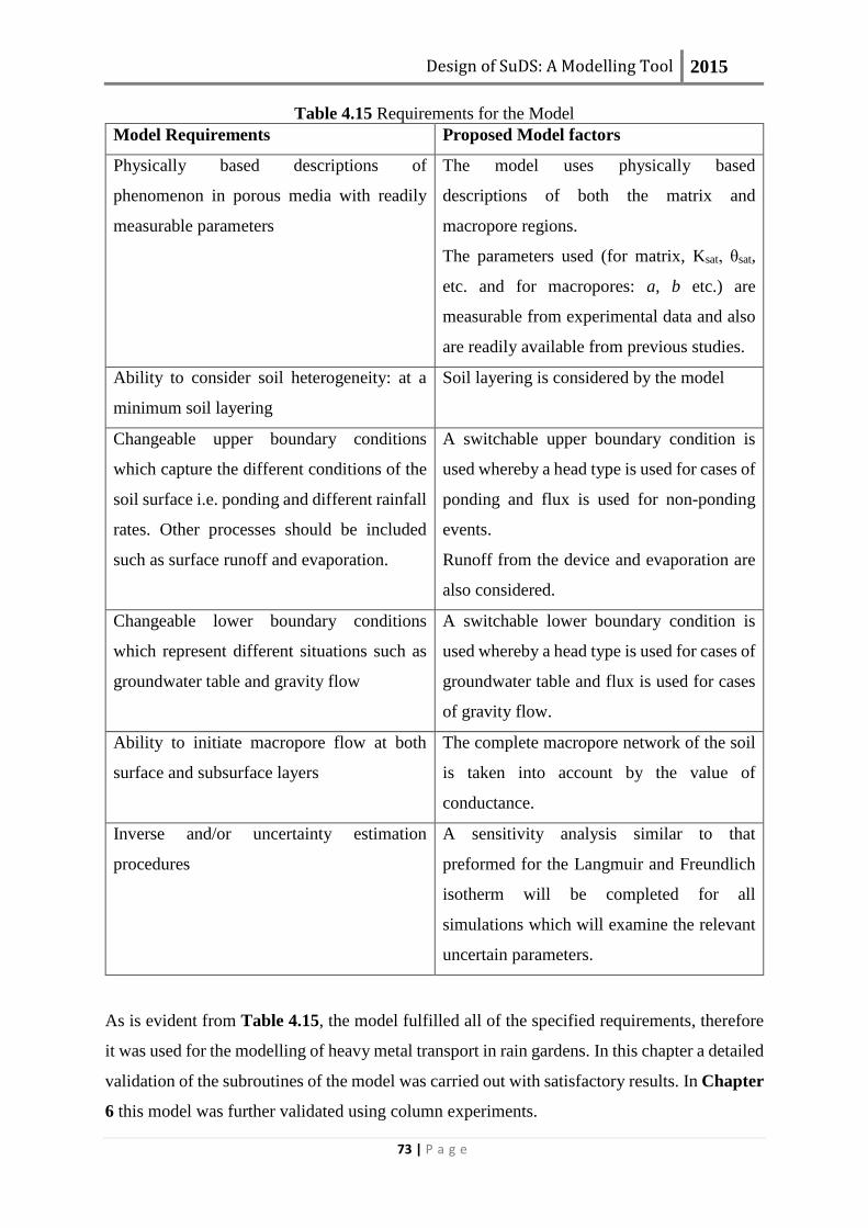
Design of SuDS: A Modelling Tool 2015
73 | P a g e
Table 4.15 Requirements for the Model
Model Requirements Proposed Model factors
Physically based descriptions of
phenomenon in porous media with readily
measurable parameters
The model uses physically based
descriptions of both the matrix and
macropore regions.
The parameters used (for matrix, Ksat, θsat,
etc. and for macropores: a, b etc.) are
measurable from experimental data and also
are readily available from previous studies.
Ability to consider soil heterogeneity: at a
minimum soil layering
Soil layering is considered by the model
Changeable upper boundary conditions
which capture the different conditions of the
soil surface i.e. ponding and different rainfall
rates. Other processes should be included
such as surface runoff and evaporation.
A switchable upper boundary condition is
used whereby a head type is used for cases of
ponding and flux is used for non-ponding
events.
Runoff from the device and evaporation are
also considered.
Changeable lower boundary conditions
which represent different situations such as
groundwater table and gravity flow
A switchable lower boundary condition is
used whereby a head type is used for cases of
groundwater table and flux is used for cases
of gravity flow.
Ability to initiate macropore flow at both
surface and subsurface layers
The complete macropore network of the soil
is taken into account by the value of
conductance.
Inverse and/or uncertainty estimation
procedures
A sensitivity analysis similar to that
preformed for the Langmuir and Freundlich
isotherm will be completed for all
simulations which will examine the relevant
uncertain parameters.
As is evident from Table 4.15, the model fulfilled all of the specified requirements, therefore
it was used for the modelling of heavy metal transport in rain gardens. In this chapter a detailed
validation of the subroutines of the model was carried out with satisfactory results. In Chapter
6 this model was further validated using column experiments.

Design of SuDS: A Modelling Tool 2015
74 | P a g e
5 COLUMN EXPERIMENTS:
DESIGN AND RESULTS 5.1 Introduction
In order to examine the retention of heavy metals in SuDS and further validate the model a
series of experiments were performed. In this chapter the aim of the experiments is briefly
discussed, the methodology used is detailed and finally the results shown and analysed. In a
subsequent chapter (Chapter 6) a validation of the model with the experimental results is
completed.
5.2 Aim of Column Experiments
As stated in Section 1.3 a component of the second aim of this research was to use experiments
to examine aspects of a rain garden device with respect to pollutant retention. Numerous
laboratory and field experiments have previously examined heavy metal retention in a rain
garden device (Davis, et al., 2001; Hsieh & Davis, 2005; Blecken, et al., 2009). However, none
examined the influence of macropores on heavy metal retention; this was established as a key
factor in pollutant capture in the literature review (Table 3.1).
Therefore, the aim of these experiments was to investigate the effect of a single artificial
macropore on heavy metal retention in a layered soil column (with similar soil layout to a rain
garden) under typical English climatic conditions.
Soil column experiments in both the saturated and unsaturated regimes are widely used for
applied and theoretical studies in such diverse fields as transport model evaluation, fate and
transport of pesticides, explosives, microbes, heavy metals and non-aqueous phase liquids.
(Lewis & Sjostrom, 2010). Their popularity is due to their apparent simplicity and
reproducibility (Lewis & Sjostrom, 2010). In terms of heavy metal sorption studies, column
experiments have inherent advantages over other approaches such as batch studies as
mentioned in Section 4.4.4.3. A further advantage is that column experiments work at a high
solid to solution ratio close to the one encountered in a natural rain garden device (Burgisser et
al., 1993). Due to these reasons, column experiments were chosen as a suitable method for
examining heavy metal retention in rain garden soil.

Design of SuDS: A Modelling Tool 2015
75 | P a g e
A number of experiments have examined the effect of the presence of macropores on the
transport and retention of tracers in soil. It was found that in the majority of cases the macropore
acted as an active preferential pathway exclusively under saturated conditions (Lamy, et al.,
2009). However numerous studies have suggested that macropore flow occurs under both
unsaturated and saturated conditions (Nimmo, 2012).
To the author’s knowledge only one column experiment has examined the influence of
macropores on the movement of heavy metals. Camobreco et al. (1996) applied an artificial
heavy metal solution to both undisturbed (containing macropores) and homogenised soil
columns of length 35 cm. A rainfall of approximately 3 cm/day (unsaturated conditions) was
simulated for 31.5 days. It was found that the homogenised columns fully capture the metals
however the macropore columns did not. Their outflow concentrations were relatively low
however at less than 30% of the input concentration. This experiment did not fully quantify the
macropore flow in the undisturbed columns so it is unclear the extent to which bypass of the
matrix region occurs.
This experimental study will indicate whether macropore flow typically occurs in rain gardens
under both average and high intensity rainfall.
5.3 Column Experimental Design
5.3.1 Composition & Macropore Presence
The experiment consisted of five columns with length 1.2 m and diameter 0.15 m. Each with
an identical substrate composition consisting of a 30 cm lower layer of coarse sand with a 60
cm upper layer of 50% compost/50% coarse sand mix by volume, an additional 30 cm was left
clear at the top of the column to allow for ponding. The constituents of both the sand and the
compost are given in Table 5.1. This composition was chosen as it reflects a typical design of
rain gardens currently in use, the top layer mix of soil was also an optimum choice for heavy
metal retention and water infiltration (Morgan, 2011). The sand used in the experiments of
Morgan (2011) had a grain size of 220𝜇m-2000𝜇m which corresponds well with the coarse
sand used in these experiments which had a diameter of 600𝜇m-2180𝜇m. This type of soil has
a very high hydraulic conductivity and has been found to have high retentive capacity for heavy
metals. As macropores have a ‘natural speed limit’, this high hydraulic conductivity may
reduce the impact of macropore flow. However, this is representative of the hydrological
processes in real garden device. This will be discussed in the conclusion in Section 5.9.

Design of SuDS: A Modelling Tool 2015
76 | P a g e
Table 5.1 Constituents of Experimental Material
Material Description Reference
Coarse Sand 100% Natural, uncrushed
Silica Sand (Quartz) Free
from silt, clay or organic
matter.
Geological classification:
Lower Greensand, Leighton
Buzzard, Beds, UK.
Diameter: 1.18mm – 600𝜇m
A sieve test was performed,
96.6% of sand was passed
the 1mm sieve and was
retained by the 500𝜇m
sieve and 3.4% passed the
500𝜇m sieve and was
retained by the 250𝜇m sieve.
Eurocode standard sieves
were used.
(DavidBall Specialist Sand,
2013)
Compost A mix of peat moss, peat and
pinebark at a ratio of 1:1:1
Chemical Composition
Humic Matter: 0.7%
Base Saturation: 78%
Phosphorus: 199 mg/L
Potassium: 100 mg/L
Cu < 50 mg/kg
Pb < 50 mg/kg
Zn <150 mg/kg
(North Carolina Department
of Agriculture, 1995; Waste
& Resources Action
Programme, 2011)
Note: The compost consisted of peat moss, peat and pinebark. The pinebark had a maximum
length of approximately 5cm. Any large clumps of peat were broken up when filling the
columns.

Design of SuDS: A Modelling Tool 2015
77 | P a g e
A common problem for column experiments is sidewall flow. Sidewall flow is the preferential
movement of water along the column wall-soil interface bypassing the material contents of the
column. In order to mitigate this effect several approaches were used:
1. The column walls were roughened using coarse sand paper to optimize soil-column
wall adhesion as recommended by Smajstrla (1985).
2. Silicone rings were installed at 30cm intervals on the interior surface of the column
prior to the addition of soil as recommended by Corwin (2000). This redirects sidewall
flow away from the column walls if it occurs.
3. The columns were filled by the method of slurry packing, this both minimizes sidewall
flow as it eliminates the air pockets at the soil column-interface and also ensures
homogeneity of the column material. This method was deemed best practice by Oliveira
et al. (1996) and Lewis & Sjostrom (2010).
Two of the columns contained artificially created macropores which extended through both
upper and lower layers of soil. These were of 1 cm in diameter in accordance with previous
solute transport experiments (Allaire-Leung, et al., 2000). These macropores were created by
inserting a metal rod through the length of the column from top to bottom following the
procedure of Kay et al. (2005). In order to prevent collapse, this insertion process was
completed before each experimental run. It was observed that the rod was easily inserted into
the substrate each time indicating that collapse did not occur
In summary, two sets of columns were created, three with normally packed homogeneous soil
(Matrix Columns) and two with preferential pathways (Macropore Columns).
5.3.2 Input Metals
The metal contaminants in the input solution for all columns were identical as Cu, Pb and Zn
as these are the most common metals present in urban storm water and also have the greatest
detrimental effects on the environment as discussed in Section 3.5 (Brown, et al. 2000; Davis,
et al. 2001).
With regards to metal concentration, high values (compared with stormwater heavy metal
concentrations) were chosen, 10000 μg/L Cu, 10000 μg/L Pb and 30000 μg/L Zn. These values
are identical to those used by the Highways Research Group (2010) and were chosen as it
allowed the examination of a large quantity of heavy metal inflow in a short amount of time.

Design of SuDS: A Modelling Tool 2015
78 | P a g e
For example the Highways Research group examined approximately a heavy metal input
amount equating to a 100 year duration in a six month period.
5.3.3 Conditions
In these experiments it was decided to replicate two common scenarios present in rain gardens
i) average and ii) first flush rainfall. Therefore, two separate experimental simulations were
carried out which are discussed below.
Average Flow
The average flow replicates a relatively low water input rate for a relatively long period of time
(5 hours). This input water rate was determined using data from a weather monitoring station
located at Heathrow. Figure 5.1 below shows the total annual rainfall as a function of intensity.
Figure 5.1 Hourly Rainfall at Heathrow Weather Station from 1998-2008
From Figure 5.1 the average rainfall amount was decided at 10.9 mm/h (circa 90% of total
annual rainfall). This was determined to be an adequate reflection of a high average rainfall in
the London area. The average input into a rain garden is much higher however as it receives
runoff from the impervious surfaces around it. The area ratio of rain garden to impervious
surface (see Section 2.6) was chosen as 10% as this was found to yield the most beneficial

Design of SuDS: A Modelling Tool 2015
79 | P a g e
results in a climate such as that of the U.K (Dussaillant, et al., 2005). This results in a total
water input of 120 mm/h.
First Flush
The first flush experiment simulated conditions where there was an extremely high intensity
rainfall following a long period of dryness. In this case the columns were allowed to drain for
a period of days prior to the start of the experimental run. The value of this high intensity
rainfall was again determined using data obtained from a weather monitoring station at
Heathrow as shown in the Figure 5.2 below.
Figure 5.2 Hourly rainfall (mm) at Heathrow from 13/10/04 to 14/10/04
The highest observed rainfall rate was 31.8 mm/h thus a column input rate of between 0 and
31.8 mm/h for 1.5 hours was chosen. As stated previously an area ratio of 10% was chosen so
this equates to a column inflow of 350 mm/h. This inflow provided a close to soil saturation
scenario for examination of macropore flow activity.
5.3.4 Instrumentation
A number of sensors were installed throughout the columns. In order to measure soil water
content eight CS645-L 3-Rod 7.5cm time domain reflectometry (TDR) probes were installed
through three of the columns (Column 1 (Macropore Column), Column 2 (Matrix Column) and
Column 5 (Macropore Column)). The probes function as a wave guide with reflections of the
applied signal along the wave guide happen when the impedance changes. The impedance is
directly related to the soil moisture content thus changes in this value result in changes in the
0
5
10
15
20
25
30
35
20
:00
:00
21
:00
:00
21
:00
:00
22
:00
:00
23
:00
:00
00
:00
:00
01
:00
:00
02
:00
:00
03
:00
:00
04
:00
:00
05
:00
:00
06
:00
:00
07
:00
:00
08
:00
:00
09
:00
:00
09
:00
:00
10
:00
:00
11
:00
:00
12
:00
:00
13
:00
:00
14
:00
:00
Ra
infa
ll (
mm
)
Time

Design of SuDS: A Modelling Tool 2015
80 | P a g e
shape of the reflection (Campbell Scientific, Inc., 2010). The shape of the reflection therefore
contains the information required for calculation of the water content.
The probes were inserted vertically through specially designed openings in the columns’ walls
following the procedure detailed by Campbell Scientific, Inc. (2013). Care was taken to
minimize soil compaction around the rods as this can lead to errors in the measurements.
To measure water head, eight 229-L water matric potential (WMP) sensors were installed
throughout three of the columns (Column 1 (Macropore Column), Column 2 (Matrix Column)
and Column 5 (Macropore Column)), as close as possible to the TDR probes so that the values
obtained were at consistent locations. A diagram of the columns and sensor positions is given
in Figure 5.3. These sensors used a heat dissipation method to indirectly measure water head
and so required a constant current source. A CE8 current excitation module was used in these
experiments.
The sensors were coated in silica flour before insertion into the columns to ensure good contact
between soil and sensor. They were installed following the procedure of Campbell Scientific,
Inc. (2009).
The water outflow rate from the base of each column was measured using a tipping bucket rain
gauge (Two Environmental Measurement Ltd. Golden River 2 mm tip rain gauges, one Texas
Instrumentation TR-525M rain gauge, one ADCON RG1 rain gauge and one ONSET 2 mm
tip rain gauge). Tipping bucket rain gauges consist of a funnel that collects and channels the
precipitation into a small seesaw-like container. After a pre-set amount of precipitation falls,
the lever tips, dumping the collected water and sending an electrical signal which is recorded
by the datalogger.
The TDR probes, WMP sensors and rain gauges were connected to a datalogger where their
measurements were stored.

Design of SuDS: A Modelling Tool 2015
81 | P a g e
Column 2 (Matrix) Column 1 (Macropore) Column 3 (Matrix)
Column 5 (Macropore) (Instrumented Column) Column 4 (Macropore)
(Instrumented Columns) (Not Instrumented Columns)
Figure 5.3 Diagram of Column Experiments. All units in mm.
5.3.5 Calibration of Instrumentation
Both types of sensors required calibration before use.
The TDR probes were calibrated using the Campbell Scientific software programme PCTDR.
For each probe the waveform length is adjusted until an accurate and clear reading is obtained.
The waveform lengths vary slightly between probes so this calibration is necessary. Further

Design of SuDS: A Modelling Tool 2015
82 | P a g e
information regarding this method is available from Campbell Scientific, Inc. (2010). An
example of the calibration procedure is contained in Appendix C1.
The WMP sensors were calibrated by inserting them in a column with the soil/sand mix or sand
(depending of their respective location). An ELE International jet fill 300mm long tensiometer
which gave water head measurements was inserted at a similar depth to the sensors. The column
was then saturated and allowed to dry. Readings were taken of the tensiometer and WMP and
compared thus calibrating the sensors. Further information regarding the calibration of WMP
sensors is available from Campbell Scientific, Inc. (2009). An example of the calibration
procedure is contained in Appendix C2.
5.3.6 Programming
The TDR probes and WMP sensors both require signals for the datalogger. These signals are
made possible by programming the datalogger. The rain gauges were also programmed but this
was separate from the probes. The pseudocode for the programming code used is given in
Appendix C4.
5.3.7 Tracer
To determine whether preferential flow has occurred a tracer (Bromide) was applied to the
column. Its outflow was monitored using a Cole-Parmer Bromide Ion Combination Epoxy
Electrode and from the breakthrough curves the degree of macropore flow was ascertained
(Cole-Parmer, 2008).
5.3.8 Summary
A summary of the experimental conditions and sensor locations is given in Table 5.2 and
illustrated in Figure 5.3.

Design of SuDS: A Modelling Tool 2015
83 | P a g e
Table 5.2 Summary of Designed Column Experiments
Column
No.
Column
Title
Diameter of
Column
Upper
Boundary
Flow
Condition
Lower
Boundary
Flow
Condition
Upper Boundary
Metal Concentration
Condition
TDR
Positions
WMP
Sensors
Positions Internal External
1 Macropore
0.14 m
0.15 m
Average Flow:
10 cm/h
First Flush:
35 cm/h
Free Flow
Measured with
Rain Gauge
10000 μg/L Cu
10000 μg/L Pb
30000 μg/L Zn
At 15cm,
55 cm, depth
At 10 cm,
50 cm depth
2 Matrix At 15 cm,
55 cm, 75cm
depth
At 10cm,
50 cm, 70 cm
depth
3 Matrix N/A N/A
4 Matrix N/A N/A
5 Macropore At 15 cm,
55 cm, 75 cm
depth
At 10 cm,
50 cm, 70 cm
depth

Design of SuDS: A Modelling Tool 2015
84 | P a g e
5.4 Methodology
The experimental set up is shown in Figure 5.4 with the inflow being delivered via sprinklers
with adjustable flow rates.
Figure 5.4 Experimental Layout

Design of SuDS: A Modelling Tool 2015
85 | P a g e
5.4.1 Average Flow Experiment
1. Solutions were prepared of 1000000 μg/L Cu, Pb and Zn using copper sulphate
(CuSO4), lead chloride (PbCl2) and zinc chloride (ZnCl2). These were then added to
deionised water to create a solution of 10000 μg/L of Cu and Pb and 30000 μg/L of Zn.
In addition, the tracer potassium bromide (KBr) (Section 5.3.7) was added at a
concentration of 1000000 μg/L. This became the inflow solution. The inflow solution
was added to the storage tank.
2. Before the start of the experiment initial readings were taken of temperature in the upper
soil of the column using a thermometer.
3. Upon commencement of the experiment the pump was switched on and the adjustable
sprinklers set to a rate of 120 mm/h. This was constantly checked throughout the course
of the experiment.
4. Measurements of soil water content and water head were taken automatically at 15
minute intervals. Soil temperature readings were taken every hour.
5. One 20 ml sample of water outflow was taken on breakthrough from the base of each
column and every hour subsequently. The concentration of Br in the sample was tested
using a Combination Ion Selective Electrode. Nitric acid was then added to the outflow
samples to preserve them and they were delivered to the laboratory for heavy metal
analysis.
6. After 5 hours the inflow ceased and the final outflow samples taken. The columns were
then allowed to completely drain out.
7. This was repeated on four separate days.
5.4.2 First Flush Experiment
Steps 1-6 were followed as above however the inflow rate was set to 350mm/h and the inflow
was ceased after 1.5 hours. This was not repeated.
The above run of experiments were repeated two more times with the soil replaced each time.
This resulted in two more experimental sets comprising of four average flow runs and one
first flush run. The first set focused on examining the hydrological parameters and heavy
metal outflow concentrations. The second and third experimental sets principally examined
the heavy metal outflow concentrations. There were minor differences in the procedure of
each of the sets, this is discussed in Section 5.7.

Design of SuDS: A Modelling Tool 2015
86 | P a g e
5.4.3 Heavy Metal Testing
All samples were sent to the Consultancy Laboratory at the University of Greenwich for
analysis. Determinations were by ICP-MS (Thermo X series II). Calibration was via synthetic
standards. The magnitude of error was 5% for this equipment and the level of detection was
0.03 μg/L for Cu, 0.01 μg/L for Pb and 0.1 μg/L for Zn (Prof D. Wray, Personal
Communication, 18/06/14). This allowed for highly accurate results and the analysis of minute
difference between matrix and macropore columns.
5.5 Results
5.5.1 Hydrological Results for Experimental Set 1
The aim of the experiments was to investigate the effect of a single artificial macropore on
heavy metal retention in a layered soil column (with similar soil layout to a rain garden) under
typical English climatic conditions. Thus it is important to ascertain whether macropore flow
had an impact on the hydrological results of soil moisture content, tracer concentration and
breakthrough time. General hydrological parameters are given in Table 5.3 for comparison
with results.
Table 5.3 Hydrological Parameters of the Columns
Parameter Sand/ Soil Mix Sand
Column 1
(Macropore
Column)
Column 2
(Matrix
Column)
Column 5
(Macropore
Column)
Column 2
(Matrix
Column)
Column 5
(Macropore
Column)
θsat (m3/m3)
(Saturated Soil
Moisture Content)
0.466
0.491
0.467
0.306
0.343
Ksat (cm/h)
(Saturated Hydraulic
Conductivity)
77 77 77 110 110
5.5.1.1 Average Flow
The labels and positions of the TDR sensors used are listed in Table 5.4.

Design of SuDS: A Modelling Tool 2015
87 | P a g e
Table 5.4 Labels and Position of TDR Sensors in Columns
TDR Sensors Column Position
1 5 (Macropore) 15 cm Depth Soil/Sand Upper Layer
2 5 (Macropore) 55 cm Depth Soil/Sand Upper Layer
3 2 (Matrix) 15 cm Depth Soil/Sand Upper Layer
4 2 (Matrix) 55 cm Depth Soil/Sand Upper Layer
5 1 (Macropore) 15 cm Depth Soil/Sand Upper Layer
6 1 (Macropore) 55 cm Depth Soil/Sand Upper Layer
7 5 (Macropore) 75 cm Depth Sand Lower Layer
8 2 (Matrix) 75 cm Depth Sand Lower Layer
Soil Moisture Content
In order to determine whether macropore flow occurred, soil moisture results of macropore and
matrix columns were examined (Figure 5.5).

Design of SuDS: A Modelling Tool 2015
88 | P a g e
Figure 5.5 Comparison of Soil Moisture Content in Column 2 (Matrix) and Column 5
(Macropore). Run 3.
If the results are compared to the θsat values contained in Table 5.3, it can be seen that the soil
moisture content is not near to saturation, thus macropore flow should not be expected to occur
in line with other column experiments (Lamy, et al., 2009).
As can be seen from Figure 5.5 at a depth of 15 cm and 75 cm the soil moisture contents in the
columns are comparable. It is noted however that at 55 cm there is a distinct difference in the
residual water content values with Column 5 (Macropore) having a considerably larger value
than Column 2 (Matrix) at all times. This could be due to macropore flow or heterogeneity of
the soil. In order to determine the cause of this discrepancy, the results of Column 2 were
compared with the other macropore column (Column 1); the results are shown in
0
0.05
0.1
0.15
0.2
0.25
0.3
0.35
0
76
20
4
33
2
46
0
58
8
71
6
84
4
97
2
11
00
12
28
13
56
14
84
Soil
Mo
istu
re C
on
ten
t (m
3 /m
3 )
Time after Start of Experiment (min)
TDR 3 (Matrix SoilDepth 15cm)
TDR 4 (Matrix SoilDepth 55cm)
TDR 8 (Matrix SandDepth 75cm)
TDR 1 (Macropore SoilDepth 15cm)
TDR 2 (Macropore SoilDepth 55cm)
TDR (Macropore SandDepth 75cm)

Design of SuDS: A Modelling Tool 2015
89 | P a g e
Figure 5.6 Comparison of Soil Moisture Content in Column 2 (Matrix) and Column 1
(Macropore). Run 3.
It is clear that there is no significant difference between the soil moisture contents in the
macropore and matrix columns. This indicates that the previous anomalous value might be due
to soil packing issues. This is supported by comparison between the TDR values at 75 cm, the
soil moisture in Column 5 displays a larger result but not later in time, this indicate that there
could be voids in the sand around TDR 8 resulting in the lower value. Without further
instrumentation it is impossible to correctly determine the cause of this deviation, thus if any
further experiments examining hydraulic properties were carried out using this equipment
additional sensors would be installed in Columns 1 and 2.
As there was no significant difference between the values of soil moisture content between the
columns, and saturation did not happen, this indicated that macropore flow did not occur and
thus did not affect the values of soil moisture content.
Tracer Results
It was found that upon breakthrough tracer inflow concentration was equal to the tracer outflow
concentration. This indicated matrix flow and no macropore or other preferential flow activity.
Water Breakthrough Times
Water breakthrough time refers to the point at which water begins to flow from the column. If
there is a preferential channel through the soil, the water should typically travel quickly through
it and thus will have a shorter breakthrough time than a matrix column (Jury & Horton, 2004).
Table 5.5 shows the breakthrough times for each of the columns for the four runs.
0
0.05
0.1
0.15
0.2
0.25
0.3
0.35
0
76
20
4
33
2
46
0
58
8
71
6
84
4
97
2
11
00
12
28
13
56
14
84
Soil
Mo
istu
re C
on
ten
t (m
3/m
3)
Time after Start of Experiment (min)
TDR 4 (Matrix Soil55cm)
TDR 6 (Macropore Soil55cm)

Design of SuDS: A Modelling Tool 2015
90 | P a g e
Table 5.5 Breakthrough Times for Columns for Average Flow Experiment
Average
Flow
Run
Column 1
(Macropore)
Breakthrough
Time (min)
Column 2
(Matrix)
Breakthrough
Time (min)
Column 3
(Matrix)
Breakthrough
Time (min)
Column 4
(Matrix)
Breakthrough
Time (min)
Column 5
(Macropore)
Breakthrough
Time (min)
1 35 37 39 37 43
2 37 43 47 37 44
3 47 45 49 48 47
4 41 41 47 48 48
As can be seen from Table 5.5 there is no considerable difference in breakthrough times
between the columns. On average they fall within 10% difference of one another.
5.5.1.2 First Flush
Soil Moisture Content
Figure 5.7 shows a comparison of the soil moisture content between a matrix and macropore
column for the first flush experimental run. As can be seen, the values vary by a much greater
degree than in the average flow experiment. This is because at higher flow rates the differences
in hydraulic parameters such as saturated soil moisture content (Table 5.3) have a greater
impact. It was thus difficult to ascertain whether macropore flow had occurred so breakthrough
times and tracer results were examined.

Design of SuDS: A Modelling Tool 2015
91 | P a g e
Figure 5.7 Comparison of Soil Moisture Content in Column 2 (Matrix) and Column 5
(Macropore). First Flush.
Tracer Results
It was found that similar to the average flow experiments upon breakthrough tracer inflow
concentration was equal to trace outflow concentration. This indicated matrix flow and no
macropore or other preferential flow activity.
Breakthrough Times
Table 5.6 shows the breakthrough times for each of the columns for the first flush experiment.
Table 5.6 Breakthrough Times for Columns for First Flush Experiment
Column 1
(Macropore)
Breakthrough
Time (min)
Column 2
(Matrix)
Breakthrough
Time (min)
Column 3
(Matrix)
Breakthrough
Time (min)
Column 4
(Matrix)
Breakthrough
Time (min)
Column 5
(Macropore)
Breakthrough
Time (min)
18 19 22 22 24
As can be seen from the table above, there is little difference between the breakthrough times
of the columns.
0
0.05
0.1
0.15
0.2
0.25
0.3
0.35
0.4
0 200 400 600
Soil
Mo
istu
re C
on
ten
t (m
3 /m
3 )
Time After Start of Experiment (min)
TDR 3 (Matrix Soil10cm)
TDR 4 (Matrix Soil45cm)
TDR 8 (Matrix Sand70cm)
TDR 1 (Macropore Soil10cm)
TDR 2 (Macropore Soil45cm)
TDR 7 (Macropore Sand70cm)

Design of SuDS: A Modelling Tool 2015
92 | P a g e
5.5.1.3 Discussion
With regards to the average flow columns, water breakthrough times, tracer and soil moisture
content findings indicate that if macropore flow was present it did not affect water flow in the
columns. This is consistent with previous findings as the columns had not achieved saturation
(Lamy, et al., 2009). This supports the possibility of complete water transfer from macropore
to matrix region as discussed in Section 4.2.2.3.
For the first flush run, soil moisture content differed between the macropore and matrix column
indicating that different flow phenomena were happening in each. This finding was not
supported by the tracer and breakthrough results, however this may be related to soil
compaction or characteristics (see Section 5.5.1.2).
It should be noted that the hydraulic conductivities of both the upper (soil/sand mix) and lower
(sand) layer are very high with a saturated hydraulic conductivity value of 77 cm/h and 110
cm/h respectively. These values are properties of the soil and was calculated by examining the
velocity of the wetting wave using the TDR results. It has been proposed by Nimmo (2007)
that macropores in soils have a ‘natural speed limit’. This limit varies depending on soil type
but has been found to range from 4.16 cm/h to 250 cm/h. The minimum breakthrough times
for the columns (Average Flow Run 3: 49 minutes Column 3, First Flush Run: 24 minutes
Column 5) indicate that the water velocity through the columns was 110 cm/h for average flow
and 225 cm/h for first flush. This is within these speed limits. Thus water could be active in the
macropores, yet have the same speed as flow in the matrix region, thus would explain the
similar breakthrough and tracer results yet the deviation in soil moisture content.
5.5.2 Heavy Metal Results for Experimental Set 1
The results of the average flow experiments are examined here as these were repeated four
times thus allowing for statistical analysis. The results of the first flush run are shown in
Appendix D6. Before the experiments were started, blank samples (containing no heavy
metals) of outflow needed to be obtained for the heavy metal chemical analysis. This was
achieved by inundating the columns with a high flow (500 mm/h) of deionised water for 1 hour.
A high flow was used as this would produce a washout of heavy metals present in the substrate.
Blank samples were collected from each of the columns, their ranges and averages are shown
in Table 5.7.

Design of SuDS: A Modelling Tool 2015
93 | P a g e
Table 5.7 Blank Sample Range and Average for Experimental Set 1
Heavy Metal Range (μg/L) Average (μg/L)
Cu 2.06-5.56 3.07
Pb 0.76-1.04 0.85
Zn 22.30-93.45 38.88
In the following figures the results of the four experimental runs are shown and heavy metal
outflow concentration is displayed as a function of experimental time (along the four runs). A
summary of the initial conditions is given in Table 5.8. Each run lasted 5 hours, there was a
period of 48 hours between Run 1 and Run 2, 96 hours between Run 2 and Run 3 and 48 hours
between Run 3 and Run 4. However soil initial conditions remained similar with a small
decrease in soil moisture content for Run 3 owing to the additional drying time (see Table 5.8).
Table 5.8 Initial Conditions for Each of the Average Flow Experimental Runs
Column Position Initial Soil Moisture Content (m3/m3)
Run 1 Run 2 Run 3 Run 4
Column 1
(Macropore)
Sand/Soil 15 cm 0.155 0.113 0.089 0.102
Sand/Soil 55 cm 0.165 0.163 0.157 0.156
Column 2
(Matrix)
Sand/Soil 15 cm 0.121 0.129 0.117 0.12
Sand/Soil 55 cm 0.146 0.147 0.138 0.145
Sand 75 cm 0.02 0.022 0.017 0.016
Column 5
(Macropore)
Sand/Soil 15 cm 0.135 0.141 0.123 .136
Sand/Soil 55 cm 0.193 0.2 0.197 .205
Sand 75 cm 0.026 0.023 0.021 .024
Cu
Figure 5.8 shows the Cu outflow results for the five columns over the accumulated
experimental time.

Design of SuDS: A Modelling Tool 2015
94 | P a g e
Figure 5.8 Cu Outflow Results
It is clear from Figure 5.8 that the Cu outflow is incredibly small compared to the inflow (2-
5.5 μg/L vs. 10000 μg/L). It is also evident that there is a trend of increasing outflow
concentration over time.
Pb
Figure 5.9 shows the Pb outflow results for the five columns over the accumulated
experimental time.
Figure 5.9 Pb Outflow Results
0.00
1.00
2.00
3.00
4.00
5.00
6.00
0 500 1000
Ou
tle
t C
u C
on
cen
trat
ion
(μ
g/L)
Time (Min)
Column 1 (Macropore)
Column 2 (Matrix)
Column 3 (Matrix)
Column 4 (Matrix)
Column 5 (Macropore)
Average BackgroundConcentration
Level of Detection
0.00
20.00
40.00
60.00
80.00
100.00
0 500 1000
Ou
tle
t P
b C
on
cen
trat
ion
(μ
g/L)
Time (Min)
Column 1 (Macropore)
Column 2 (Matrix)
Column 3 (Matrix)
Column 4 (Macropore)
Column 5 (Macropore)
Average BackgroundConcentration
Level of Detection

Design of SuDS: A Modelling Tool 2015
95 | P a g e
It is clear from Figure 5.9 that the Pb outflow is incredibly small compared to the inflow (0.23-
95 μg/L vs. 10000μg/L). There is a rapid rise in outflow concentration at the start of the
experimental time following this, the results become almost constant with a slight increase.
There is an unexplained decrease in Pb outflow concentration for the final sample this is
attributed to human error or additional sediment present in the sample collected. The high initial
values from Column 4 are attributed to early flush out of Pb from the soil. This is supported by
the values of the original blank sample from this column which was 1.04 μg/L compared to an
average of 0.70 μg/L for the other columns. Inconsistent results were also observed in Column
3; it was difficult to ascertain the cause of these anomalies as this column was not instrumented.
However it was observed that there were numerous voids in the columns allowing for sidewall
flow (a form of preferential flow).
Zn
Figure 5.10 shows the Zn outflow results for the five columns over the accumulated
experimental time.
Figure 5.10 Zn Outflow Results
It is evident from Figure 5.10 that the Zn outflow is incredibly small compared to the inflow
(7-130 μg/L vs. 30000 μg/L). There is a very slight increase in concentration over time however
similar to Pb, there is a decrease in outflow concentration towards the end of the experiment.
Although it is clear from the results that the columns showed excellent retention of heavy
metals, it is less apparent as to whether there is a dramatic difference in outflow between the
0.00
20.00
40.00
60.00
80.00
100.00
120.00
140.00
0 500 1000
Ou
tle
t Zn
Co
nce
ntr
atio
n (μ
g/L)
Time (min)
Column 1 (Macropore)
Column 2 (Matrix)
Column 3 (Matrix)
Column 4 (Macropore)
Column 5 (Macropore)
Average BackgroundConcentration
Level of Detection

Design of SuDS: A Modelling Tool 2015
96 | P a g e
different runs and also the different columns. This was the primary reason that statistical
analysis was completed.
5.6 Statistical Analysis of Heavy Metal Results
In the following section daily average outflow concentration graphs are displayed. The error
bars represent the maximum and minimum concentration values of samples in their respective
runs.
Cu
Figure 5.11 shows the plot of mean outflow of the runs for the five columns.
Figure 5.11 Plot of Cu Outflow Mean for the Different Columns.
The above plot clearly shows that similar behaviour can be seen in macropore columns (1 and
5) and in two of the matrix columns (2 and 4). This demonstrates that although preliminary
results for soil moisture content and water outflow indicated that macopore flow did not have
an impact on hydraulic parameters (Section 5.5.1), it did influence Cu transport.
Pb
Figure 5.12 shows the plot of mean outflow of the runs for the five columns.
0
1
2
3
4
5
6
1 2 3 4
Ou
tle
t C
u C
on
cen
trat
ion
(μ
g/L)
Run
Column 1 (Macropore)
Column 2 (Matrix)
Column 3 (Matrix)
Column 4 (Matrix)
Column 5 (Macropore)
Average BackgroundConcentration
Level of Detection

Design of SuDS: A Modelling Tool 2015
97 | P a g e
Figure 5.12 Plot of Pb Outflow Mean for the Different Columns.
For the case of Pb high similarity is observed between all columns, except for two exceptionally
high concentrations for Column 4 (Run 1) and Column 3 (Run 2). This is attributed to the same
reasons as discussed above for Cu. Again Column 4 had a high blank concentration of 30 μg/L
compared to an average of 22 μg/L for the other columns.
Zn
Figure 5.13 shows the plot of mean outflow of the runs for the five columns.
Figure 5.13 Plot of Zn Outflow Mean for the Different Columns.
0
20
40
60
80
100
120
1 2 3 4
Ou
tle
t P
b C
on
cen
trat
ion
(μ
g/L)
Run
Column 1 (Macropore)
Column 2 (Matrix)
Column 3 (Matrix)
Column 4 (Matrix)
Column 5 (Macropore)
Average BackgroundConcentration
Level of Detection
0
20
40
60
80
100
120
140
1 2 3 4
Ou
tle
t Zn
Co
nce
ntr
atio
n (μ
g/L)
Run
Column 1 (Macropore)
Column 2 (Matrix)
Column 3 (Matrix)
Column 4 (Matrix)
Column 5 (Macropore)
Average BackgroundConcentration
Level of Detection

Design of SuDS: A Modelling Tool 2015
98 | P a g e
With Zn there is no discernible pattern between the different types of columns.
5.6.1 T-test (P-value)
The basic t-test (or p-value testing) is the comparison of a t-distribution plot in which the null
or alternative hypothesis is proven to be true. In simple terms, the t-test compares the actual
difference between two means in relation to the variation in the data (expressed as the standard
deviation of the difference between the means).
Two different t-tests were completed; the results are found below.
T-test comparison of columns over different days
Purpose: To compare the runs for the individual columns to investigate whether the outflow
concentration increases with time.
1: State hypotheses
Null Hypotheses: Outflow concentration does not change over the runs.
Alternative Hypothesis: Outflow concentration does change over the runs
2: Formulate an analysis plan
Significance level: In accordance with generally accepted values
𝑃 < 0.01 Very strong presumption against null hypotheses (Highly statistically
significant)
0.01 < 𝑃 < 0.05 Strong presumption against null hypotheses (Statistically significant)
0.05 < 𝑃 < 0.1 Low presumption against null hypotheses (Low statistical significance)
𝑃 > 0.1 No presumption against null hypotheses (Not statically significant)
Test method: Paired t-test – data is not independent
3: Analyse Sample Data
Cu
Table 5.9 shows the p-values for the different columns over the experimental runs for Cu.
These values are derived from the t-distributions of all the outflow concentrations obtained on
each of the individual runs. It is clear that although the preliminary results (Section 5.4.2)
indicated that there is no evidence of macropore flow in any of the columns, the p-values
indicate that there is a strong presumption against the null hypothesis for Columns 1 and 5

Design of SuDS: A Modelling Tool 2015
99 | P a g e
(Macropore) and Column 3 (Matrix) across the runs (comparison of Run 1-4). For Column 1
and 5 this can be due to the macropores present; it is attributed to sidewall flow in Column 3.
These results further reinforce the trend indicated in Figure 5.11. This may be due to Cu
moving through the macropore channels; Cu is the most water-mobile of the heavy metals so
even if just a small concentration were present in the macropores it would not be retained to
the same extent as in the matrix region as macropores have a lower retentive capacity.
Table 5.9 P-values for Experimental Runs for Cu.
Column Run 1-2 Run 1-3 Run 1-4 Run 2-3 Run 2-4 Run 3-4
Column 1
(Macropore)
0.7020 0.8339 0.0211
Significant
0.9314 0.0172
Significant
0.1903
Column 2
(Matrix)
0.7186 0.0534
Low
Significance
0.2542 0.0099
High
Significance
0.1175 0.1903
Column 3
(Matrix)
0.0965
Low
Significance
0.0238
Significant
0.0319
Significant
0.2012 0.1660 0.4908
Column 4
(Matrix)
0.6889 0.1891 0.2063 0.2008 0.2895 0.3640
Column 5
(Macropore)
0.1514 0.8549 0.0088
High
Significance
0.4845 0.0026
High
Significance
0.0527
Low
Significance
Pb
Table 5.10 shows the p-values for the different columns over the experimental runs for Pb.
In general Pb is considered to be a very immobile heavy metal in the soil columns (Li & Davis,
2008). This is supported by the findings of the p-values which predominately support the null
hypothesis for each column. There was a problem however with the values obtained for Run 4
which were abnormally low compared to previous results. This explains the low p-values for
the comparison of Runs 1, 2 and 3 to Run 4. There are however two p-values which reject the
null hypothesis, these are predominately limited to the macropore columns (Column 1 and
Column 5).

Design of SuDS: A Modelling Tool 2015
100 | P a g e
Table 5.10 P-values for Experimental Runs for Pb.
Column Run 1-2 Run 1-3 Run 1-4 Run 2-3 Run 2-4 Run 3-4
Column 1
(Macropore)
0.953 0.9669 0.3023 0.2916 0.0715
Low
Significance
0.4331
Column 2
(Matrix)
0.4287 0.488 0.9321 0.6065 0.3106 0.4165
Column 3
(Matrix)
0.3317 0.210 0.5097 0.4299 0.2718 0.1813
Column 4
(Matrix)
0.3336 0.3272 0.2409 0.8275 0.1404 0.1601
Column 5
(Macropore)
0.6862 0.4221 0.1527 0.2004 0.0378
Significant
0.2457
Zn
Table 5.11 shows the p-values for the different columns over the experimental runs for Zn.
The results for the p-values in the majority of cases agree with the null hypothesis. This is
attributed to the immobility of Zn in the soil column. It is observed that the outflow of Zn was
very low on Run 4, which could indicate some problems having occurred such as an incorrect
amount of nitric acid being added thus allowing the heavy metals to sorb to the sample bottle
walls decreasing the concentration.

Design of SuDS: A Modelling Tool 2015
101 | P a g e
Table 5.11 P-values for Experimental Runs for Zn.
Column Run 1-2 Run 1-3 Run 1-4 Run 2-3 Run 2-4 Run 3-4
Column 1
(Macropore)
0.0777
Low
Significance
0.0853
Low
Significance
0.3914 0.7715 0.1432 0.3044
Column 2
(Matrix)
0.1061 0.0889
Low
Significance
0.1853 0.2291 0.7368 0.3931
Column 3
(Matrix)
0.1442 0.1010 0.6208 0.2851 0.1083 0.1578
Column 4
(Matrix)
0.4504 0.7879 0.3453 0.0201
Significant
0.7650 0.0872
Column 5
(Macropore)
0.0438
Significant
0.4740 0.8885 0.7369 0.6147 0.2476
Conclusion
It is clear from the results of the p-values that only Cu increases with time. This is to be
expected; as stated the experimental duration was short and Cu was the most mobile heavy
metal (Davis, et al., 2001), therefore the most likely to increase in outflow concentration over
the limited time of these experiments.
T-test comparison of columns with Each Other on Same Day
Purpose: To examine whether columns with the same and different characteristics
(matrix/macropore) have similar outflow concentrations i.e. are the results consistent and does
macropore flow impact pollutant retention compared with matrix columns.
Step 1: State hypotheses
Null Hypotheses: Outflow concentration does not change between columns
Alternative Hypothesis: Outflow concentration does change between columns
Step 2: Formulate an analysis plan
Significance level: In accordance with generally accepted values
P< 0.01 very strong presumption against null hypotheses

Design of SuDS: A Modelling Tool 2015
102 | P a g e
0.01<P<0.05 strong presumption against null hypotheses
0.05<P<0.1 low presumption against null hypotheses
P>0.1 no presumption against null hypotheses
Test method: Unpaired t-test – data is independent
Step 3: Analyse Sample Data
Cu
Comparing Columns with Similar Characteristics
Table 5.12 shows the p-values for a comparison between columns with the same characteristics
over the four runs for Cu.
Table 5.12 P-values for Columns with Similar Characteristics for Cu
Macropore
Columns
Matrix Columns
Column 1-5 Column 2-3 Column 2-4 Column 3-4
Run 1 0.6259 0.4613 0.2766 0.9592
Run 2 0.5704 0.0126
Significant
0.6785 0.1288
Run 3 0.8900 0.2904 0.7567 0.436
Run 4 0.7962 0.0886
Low
Significance
0.7727 0.0900
Low
Significance
It was found for the case of similar columns i.e. when matrix columns (2-4) were compared to
matrix columns and when macropore columns (1 and 5) were compared to macropore columns
there was no presumption against the null hypothesis. This indicated that the results of the
matrix and macropore columns were consistent within their type. There was one exception
however, of Column 2 compared with Column 3 for Run 2, as stated previously there were
some problems with Column 3 which were attributed to sidewall flow.

Design of SuDS: A Modelling Tool 2015
103 | P a g e
Comparing Columns with Different Characteristics
Table 5.13 shows the p-values for a comparison between columns with different characteristics
over the four runs for Cu.
Table 5.13 P-values for Columns with Different Characteristics for Cu
Column
1-2
Column
1-3
Column
1- 4
Column
5-2
Column
5-3
Column
5-4
Run 1 0.5319 0.9722 1 0.0523
Low
Significance
0.4941 0.3345
Run 2 0.4752 0.4038 0.720 0.8337 0.0375
Significant
0.8152
Run 3 0.4904 0.1645 0.3783 0.4963 0.1404 0.3646
Run 4 0.0712
Low
Significance
0.7929 0.0615
Low
Significance
0.0225
Significant
0.6161 0.0042
Highly
Significant
It is clear that the difference in outflow concentration between macrocpore columns (1 and 5)
and matrix columns (2-4) becomes significant in run 4. This is also clearly illustrated by
Figure 5.11.
Pb
Table 5.14 and Table 5.15 show the p-values for a comparison between the columns with
similar and different characteristics over the four runs for Pb respectively.

Design of SuDS: A Modelling Tool 2015
104 | P a g e
Table 5.14 P-values for Columns with Similar Characteristics for Pb
Macropore
Columns
Matrix Columns
Column 1-5 Column 2-3 Column 2-4 Column 3-4
Run 1 0.7804 0.9827 0.2551 0.2579
Run 2 0.4897 0.3478 0.7257 0.3394
Run 3 0.3725 0.2968 0.3410 0.2260
Run 4 0.5098 0.5063 0.4807 0.9755
Table 5.15 P-values for Columns with Different Characteristics for Pb
Column
1-2
Column
1-3
Column
1- 4
Column
5-2
Column
5-3
Column
5-4
Run 1 0.6109 0.6616 0.2867 0.3976 0.4750 0.2994
Run 2 0.3779 0.3974 0.2700 0.7163 0.3584 0.4048
Run 3 0.6712 0.2216 0.7883 0.3095 0.1464 0.3410
Run 4 0.8384 0.6651 0.6398 0.3556 0.8387 0.8622
For Pb in all cases, there is no presumption against the null hypothesis. This is attributed to
the immobility of Pb in soils (Li & Davis 2008)
Zn
Table 5.16 and Table 5.17 show the p-values for a comparison between the columns with
similar and different characteristics over the four runs for Zn respectively.

Design of SuDS: A Modelling Tool 2015
105 | P a g e
Table 5.16 P-values for Columns with Similar Characteristics for Zn
Macropore
Columns
Matrix Columns
Column 1-5 Column 2-3 Column 2-4 Column 3-4
Run 1 0.8987 0.4133 0.3729 0.4289
Run 2 0.0918
Low
Significance
0.1965 0.2700 0.4755
Run 3 0.3253 0.8108 0.8795 0.9232
Run 4 0.5308 0.3106 0.3895 0.9232
Table 5.17 P-values for Columns with Different Characteristics for Zn
Column
1-2
Column
1-3
Column
1- 4
Column
5-2
Column
5-3
Column
5-4
Run 1 0.7406 0.1012 0.3506 0.7905 0.1102 0.3546
Run 2 0.2225 0.8865 0.1045 0.1468 0.0609
Low
Significance
0.9494
Run 3 0.9724 0.8254 0.9010 0.3430 0.3162 0.3329
Run 4 0.6768 0.5540 0.6488 0.2869 0.9851 0.8884
For the majority of Zn case, there is no significant presumption against the null hypothesis.
This is attributed to the immobility of Zn in soils (Li & Davis, 2008).
Conclusion
For the case of Pb and Zn the null hypothesis was proven. However for the case of Cu the most
mobile heavy metal, it was shown that although the null hypothesis was proven for Runs 1-3,
the alternative hypothesis was true for Run 4. This indicates that with increasing time and
inflow the outlet concentration of macropore columns is greater than matrix columns. More
research is needed into this phenomenon and longer duration experiments should be carried out
in the future in order to conclusively prove that the Cu outflow increases in macropore columns
over time.

Design of SuDS: A Modelling Tool 2015
106 | P a g e
5.6.2 ANOVA concept
ANOVA (ANalyis Of VAriants) is a method of comparing the means of several groups. It is
used when there are more than two existing groups, for which a t-test would not give
appropriate results. The groups in this case consist of the all the samples (5 samples per column
per run) taken from a column on an individual run.
ANOVA comparison of results Two-Way ANOVA
Due to similarities between the one-way ANOVA test and the p-test completed earlier it was
decided only to discuss the results of two-way ANOVA analysis.
The two explanatory variables for examination in this experiment were the different columns
and the different experimental runs. The two way test not only indicates whether there is
significant difference between the individual explanatory variables but also whether they have
an influence on one another. The ANOVA results for the different heavy metals are shown in
the following tables, Table 5.18 (Cu), Table 5.19 (Pb), Table 5.20 (Zn).
Table 5.18 Two Way ANOVA Analysis Results for Cu Outflow
ANOVA
Source of Variation P-value (Significance)
Runs 5.58E-07
(High Significance)
Columns 0.027964
(Significant)
Interaction 0.261018
Table 5.19 Two Way ANOVA Analysis Results for Pb Outflow
ANOVA
Source of Variation P-value (Significance)
Runs 0.128651
Columns 0.544997
Interaction 0.34227

Design of SuDS: A Modelling Tool 2015
107 | P a g e
Table 5.20 Two Way ANOVA Analysis Results for Zn Outflow
ANOVA
Source of Variation P-value (Significance)
Runs 0.105281
Columns 0.467761
Interaction 0.535288
As can be seen only Cu has significant p-values for both the run and column explanatory
variables. This supports the findings of both the t-test (Section 5.6.1) and the plot of means
(Figure 5.11) which show that not only does Cu outflow increase over the runs but also that
there is a significant difference in outflow between the macropore and matrix columns. There
is no substantial interaction between the columns. It is interesting to note however that it is
clear from Figure 5.11 that the difference between the outflow for macropore and matrix
columns increases with the increasing runs.
Zn and Pb do not have significant p-values for columns or interaction meaning that there is no
difference between the columns and macropore flow did not increase the outflow
concentration. The values for the runs however almost reach a low presumption against the null
hypothesis. This contradicts what was found by the t-test (Section 5.6.1) and may be due to the
extremely high and low outflow concentrations observable in Figure 5.9 and Figure 5.10 and
not due to an underlying increase in outflow. In order to ascertain whether this is the case the
two-way ANOVA test has been repeated for Pb (Table 5.21) and Zn (Table 5.22) for the first
three runs ignoring the very low values of Run 4.
Table 5.21 Two Way ANOVA Analysis for Pb Outflow for Three Runs
ANOVA
Source of Variation P-value (Significance)
Runs 0.4844
Columns 0.480098
Interaction 0.327424

Design of SuDS: A Modelling Tool 2015
108 | P a g e
Table 5.22 Two Way ANOVA Analysis for Zn Outflow for Three Runs
ANOVA
Source of Variation P-value (Significance)
Runs 0.235367
Columns 0.433453
Interaction 0.386567
It is shown from both the above tables that the p-values have increased significantly once Run
4 was removed from the comparison. This proves that the results of the t-test are valid and Pb
and Zn are retained by the columns agreeing with previous research (Davis, et al., 2003).
5.7 Results of Further Experiments
It was observed from the results of the above experiments that the outflow heavy metal
concentrations were very low and did not significantly exceed background concentrations.
Although it was found that the outflow concentration of Cu increased with time in the
macropore columns; this outflow concentration was very close to both level of detection and
background concentration. This results in a higher degree of error in analysis which may have
resulted in the unexplained spikes in outflow concentration (Figure 5.9 and Figure 5.10).
Therefore, the above experiments were repeated two more times with the soil replaced each
time. This resulted in two more experimental sets comprising of four average flow runs and
one first flush run. In order to gain a better understanding of the results obtained several
changes were made to the experimental design:
1. Ph. values were taken for each of the experimental runs.
2. Blank samples were taken over a longer period of time see Section 5.7.1.2.
3. At every sample time, 3 samples were taken instead of one.
5.7.1 Experimental Set 2
5.7.1.1 pH Results
The pH was tested using Fisherbrand pH indicator paper litmus 2 to 12 pH. It was found that
the pH ranged from 4-5 in the tank before input into the columns and 6-7 for the column
outflow. This was consistent for all runs.

Design of SuDS: A Modelling Tool 2015
109 | P a g e
5.7.1.2 Blank Samples
A preliminary run was completed in order to obtain a sizeable number of blank samples and
obtain a meaningful representation of background heavy metal concentration. This run was
identical in duration and sampling times as the average flow runs detailed in Section 5.4.1
except the input was pure distilled water without additional heavy metals. The blank sample
range and average is shown in Table 5.23, the complete blank results are given in Appendix
D5.
Table 5.23 Blank Sample Range and Average for Experimental Set 2
Heavy Metal Range Average
Cu 0.727-8.633 2.682
Pb 0.03-3.416 0.896
Zn 2.093-33.400 14.840
5.7.1.3 Results
Below are the results for experimental set 2 for the average flow runs. The results of the first
flush run are shown in Appendix D6. The initial conditions for the columns were identical to
those for experiment set 1 (Table 5.8).
Cu
Figure 5.14 shows the Cu outflow for the five columns over the experimental time.
Figure 5.14 Cu Outflow Results for Experimental Set 2
0.00
1.00
2.00
3.00
4.00
5.00
6.00
7.00
0 200 400 600 800 1000 1200
Cu
Ou
tle
t C
on
cen
trat
ion
(μ
g/L)
Time (Min)
Column 1 (Macropore)
Column 2 (Matrix)
Column 3 (Matrix)
Column 4 (Matrix)
Column 5 (Macropore)
Average BackgroundConcentration
Level of Detection

Design of SuDS: A Modelling Tool 2015
110 | P a g e
It is clear from Figure 5.14 that the Cu outflow is small compared to the inflow (0.536-5,.8
μg/L vs. 10000 μg/L). The outflow concentration remains consistent between the columns and
is approximately equal to background concentration. This indicates that the inflow heavy metal
concentrations are being retained in the columns.
Pb
Figure 5.15 shows the Pb outflow for the five columns over the experimental time.
Figure 5.15 Pb Outflow Results for Experimental Set 2
Again, the outflow concentration is small compared to inflow (0.03-6.5 μg/L vs. 10000 μg/L)
and the outflow concentration remains approximately to the background concentration.
Zn
Figure 5.16 shows the Zn outflow for the five columns over the experimental time.
0.00
1.00
2.00
3.00
4.00
5.00
6.00
7.00
55 180 300 420 560 670 780 900 10201140
Pb
Ou
tlet
Co
nce
ntr
ati
on
(μ
g/L
)
Time (Min)
Column 1 (Macropore)
Column 2 (Matrix)
Column 3 (Matrix)
Column 4 (Matrix)
Column 5 (Macropore)
BackgroundConcentration
Level of Detection

Design of SuDS: A Modelling Tool 2015
111 | P a g e
Figure 5.16 Zn Outflow Results for Experimental Set 2
Again, the outflow concentration is small compared to inflow (0.03-95 μg/L vs. 30000 μg/L)
and the outflow concentration remains approximately to the background concentration.
Plot of the Means
The plot of the means for each of the heavy metal outflow concentrations, Cu (Figure 5.17),
Pb (Figure 5.18) and Zn (Figure 5.19) supports the findings of the above.
Figure 5.17 Plot of Cu Outflow Mean for the Different Columns for Experimental Set 2
0.0
20.0
40.0
60.0
80.0
100.0
120.0
55 180 300 420 560 670 780 900 1020 1140
Zn
Ou
tlet
Co
nce
ntr
ati
on
(μ
g/L
)
Time (Min)
Column 1(Macropore)
Column 2 (Matrix)
Column 3 (Matrix)
Column 4 (Matrix)
Column 5(Macropore)
Average BackgroundConcentration
Level of Detection
0.000
1.000
2.000
3.000
4.000
5.000
6.000
7.000
1 2 3 4
Cu
Ou
tlet
Co
ncen
tra
tio
n (μ
g/L
)
Run
Column 1(Macropore)
Column 2 (Matrix)
Column 3 (Matrix)
Column 4 (Matrix)
Column 5(Macropore)
AverageBackgroundConcentrationLevel of Detection

Design of SuDS: A Modelling Tool 2015
112 | P a g e
Figure 5.18 Plot of Pb Outflow Mean for the Different Columns for Experimental Set 2
Figure 5.19 Plot of Zn Outflow Mean for the Different Columns for Experimental Set 2
Unlike the increased Cu outflow observed in Experimental Set 1, no pattern is seen from any
of the heavy metal outflows in Experimental Set 2. Therefore, it is concluded that all columns
retained the inflow concentration which supports previous experimental findings (Davis et al.
2001, Li & Davis, 2008). Therefore no statistical analysis was completed.
0.00
0.50
1.00
1.50
2.00
2.50
3.00
3.50
4.00
4.50
5.00
1 2 3 4
Pb
Ou
tle
t C
on
cen
trat
ion
(μ
g/L)
Run
Column 1 (Macropore)
Column 2 (Matrix)
Column 3 (Matrix)
Column 4 (Matrix)
Column 5 (Macropore)
Average BackgroundConcentration
Level of Detection
0.00
20.00
40.00
60.00
80.00
100.00
120.00
1 2 3 4
Zn O
utl
et
Co
nce
ntr
atio
n (μ
g/L)
Run
Column 1 (Macropore)
Column 2 (Matrix)
Column 3 (Matrix)
Column 4 (Matrix)
Column 5 (Macropore)
Average BackgroundConcentration
Level of Detection

Design of SuDS: A Modelling Tool 2015
113 | P a g e
5.7.2 Experimental Set 3
5.7.2.1 pH Results
The pH was tested using Fisherbrand pH indicator paper litmus 2 to 12 pH. It was found that
the pH ranged from 4-5 in the tank before input into the columns and 6-7 for the column
outflow. This was consistent for all runs.
5.7.2.2 Blank Samples
A preliminary run to collect blank samples was completed in an identical fashion to that
described by Section 5.7.1.2. The blank sample range and average is shown in Table 5.23, the
complete blank results are given in Appendix D5.
Table 5.24 Blank Sample Range and Average for Experimental Set 3
Heavy Metal Range (μg/L) Average (μg/L)
Cu 1.228-7.444 3.223
Pb 0.215-2.097 0.592
Zn 3.639-132.207 22.435
5.7.2.3 Results
Below are the results for experimental set 2 for the average flow runs. The results of the first
flush run are shown in Appendix D6. The initial conditions for the columns were identical to
those for experiment set 1 and 2 (Table 5.8).
The outlet concentrations of Cu, Pb and Zn for the average flow runs are shown in Figure 5.20
(Cu), Figure 5.21(Pb with outliers), Figure 5.22 (Pb without outliers) and Figure 5.23 (Zn).
It is clear that in all cases excellent retention of heavy metals is observed with the outlet
concentration staying approximately equal to the average blank concentration. There is also no
significant difference between the matrix and macropore columns, indicating the macropores
did not diminish retention.

Design of SuDS: A Modelling Tool 2015
114 | P a g e
Figure 5.20 Cu Outflow Concentration for Experimental Set 3
Figure 5.21 Pb Outflow Concentration for Experimental Set 3 with Outliers
0.00
1.00
2.00
3.00
4.00
5.00
6.00
7.00
8.00
9.00
50 550 1050
Ou
tle
t C
u C
on
cen
trat
ion
(μ
g/L
)
Time (Min)
Column 1(Macropore)
Column 2 (Matrix)
Column 3 (Matrix)
Column 4 (Matrix)
Column 5(Macropore)
Average BlankConcentration
Level of Detection
0.00
50.00
100.00
150.00
200.00
250.00
50 250 450 650 850 1050 1250
Ou
tle
t P
b C
on
cen
trat
ion
(μ
g/L
)
Time (Min)
Column 1 (Macropore)
Column 2 (Matrix)
Column 3 (Matrix)
Column 4 (Matrix)
Column 5 (Macropore)
Average BlankConcentration
Level of Detection

Design of SuDS: A Modelling Tool 2015
115 | P a g e
Figure 5.22 Pb Outflow Concentration for Experimental Set 3 without Outliers
Figure 5.23 Zn Outflow Concentration for Experimental Set 3
Plot of the Means
The plot of the means for each of the heavy metal outflow concentrations, Cu (Figure 5.17),
Pb (Figure 5.18) and Zn (Figure 5.19) supports the findings of the above.
0.00
10.00
20.00
30.00
40.00
50.00
60.00
70.00
80.00
50 250 450 650 850 1050 1250
Ou
tle
t P
b C
on
cen
trat
ion
(μ
g/L
)
Time (Min)
Column 1 (Macropore)
Column 2 (Matrix)
Column 3 (Matrix)
Column 4 (Matrix)
Column 5 (Macropore)
Average BlankConcentration
Level of Detection
0.00
20.00
40.00
60.00
80.00
100.00
120.00
140.00
50 550 1050
Ou
tle
t Zn
Co
nce
ntr
atio
n (μ
g/L
)
Time (Min)
Column 1(Macropore)
Column 2 (Matrix)
Column 3 (Matrix)
Column 4 (Matrix)
Column 5(Macropore)
Average BlankConcentration
Level of Detection

Design of SuDS: A Modelling Tool 2015
116 | P a g e
Figure 5.24 Plot of Cu Outflow Mean for the Different Columns for Experimental Set 3
Figure 5.25 Plot of Zn Outflow Mean for the Different Columns for Experimental Set 3
0.00
1.00
2.00
3.00
4.00
5.00
6.00
7.00
8.00
1 1.5 2 2.5 3 3.5 4
Ou
tle
t C
u C
on
cen
trat
ion
(μ
g/L
)
Run
Column 1(Macropore)
Column 2 (Matrix)
Column 3 (Matrix)
Column 4 (Matrix)
Column 5(Macropore)
Average BlankConcentration
Level of Detection
0
20
40
60
80
100
120
140
160
180
200
1 2 3 4
Ou
tle
t Zn
Co
nce
ntr
atio
ns
(μg
/L)
Run
Column 1(Macropore)
Column 2 (Matrix)
Column 3 (Matrix)
Column 4 (Matrix)
Column 5(Macropore)
Average BlankConcentration
Level of Detection

Design of SuDS: A Modelling Tool 2015
117 | P a g e
Figure 5.26 Plot of Pb Outflow Mean for the Different Columns for Experimental Set 3 with
Outliers
5.8 Comparisons Between Experimental Sets
In this section, the experimental sets are compared to one another in order to determine the
variability between sets.
5.8.1 Average Flow Runs
An example of comparison between sets for individual columns is given for each of the heavy
metals Figure 5.27 (Cu) Figure 5.28 (Pb) and Figure 5.29 (Zn). The remainder of the
comparisons is given in Appendix D7.
0.000
20.000
40.000
60.000
80.000
100.000
120.000
140.000
160.000
180.000
200.000
1 2 3 4
Ou
tle
t P
b C
on
cen
trat
ion
(μ
g/L
)
Run
Column 1(Macropore)
Column 2 (Matrix)
Column 3 (Matrix)
Column 4 (Matrix)
Column 5(Macropore)
Average BlankConcentration
Level of Detection

Design of SuDS: A Modelling Tool 2015
118 | P a g e
Figure 5.27 Comparison of Outflow Cu Concentration in Column 1 for Different
Experimental Sets for Average Flow Runs.
Figure 5.28 Comparison of Outflow Pb Concentration in Column 2 for Different
Experimental Sets for Average Flow Runs.
0.00
1.00
2.00
3.00
4.00
5.00
6.00
0 200 400 600 800 1000 1200
Ou
tle
t C
u C
on
cen
trat
ion
(μ
g/L
)
Time (Min)
Set 1
Set 2
Set 3
0.00
20.00
40.00
60.00
80.00
100.00
120.00
140.00
160.00
180.00
200.00
0 200 400 600 800 1000 1200
Ou
tle
t P
b C
on
cen
trat
ion
(μ
g/L
)
Time (Min)
Set 1
Set 2
Set 3

Design of SuDS: A Modelling Tool 2015
119 | P a g e
Figure 5.29 Comparison of Outflow Zn Concentration in Column 5 for Different
Experimental Sets for Average Flow Runs.
It is clear that for all cases the results of the different sets for the average flow runs are
comparable. The small variation between the sets is attributed to differences in background
concentration (Table 5.7 (Set 1) Table 5.23 (Set 2) Table 5.24 (Set 3)). This indicates the
repeatability of the experiments.
5.8.2 First Flush Runs
An example of comparison between sets for individual columns is given for each of the heavy
metals Figure 5.30 (Cu), Figure 5.31 (Pb) and Figure 5.32 (Zn). The remainder of the
comparisons is given in Appendix D8.
0.00
20.00
40.00
60.00
80.00
100.00
120.00
0 200 400 600 800 1000 1200
Ou
tle
t Zn
Co
nce
ntr
atio
n (μ
g/L
)
Time (Min)
Set 1
Set 2
Set 3

Design of SuDS: A Modelling Tool 2015
120 | P a g e
Figure 5.30 Comparison of Outflow Cu Concentration in Column 3 for Different
Experimental Sets for First Flush Flow Runs.
Figure 5.31 Comparison of Outflow Pb Concentration in Column 3 for Different
Experimental Sets for First Flush Flow Runs.
0.00
2.00
4.00
6.00
8.00
10.00
12.00
15 25 35 45 55 65 75 85 95
Ou
tle
t C
u C
on
cen
trat
ion
(μ
g/L
)
Time (Min)
Set 1
Set 2
Set 3
0.00
0.50
1.00
1.50
2.00
2.50
3.00
15 25 35 45 55 65 75 85 95
Ou
tle
t P
b C
on
cen
trat
ion
(μ
g/L
)
Time (Min)
Set 1
Set 2
Set 3

Design of SuDS: A Modelling Tool 2015
121 | P a g e
Figure 5.32 Comparison of Outflow Zn Concentration in Column 3 for Different
Experimental Sets for First Flush Flow Runs.
It is clear that for all cases the results of the different sets for the first flow flow runs are
comparable. The small variation between the sets is attributed to differences in background
concentration (Table 5.7 (Set 1) Table 5.23 (Set 2) Table 5.24 (Set 3)). However this
variability is small compared to the overall inflow heavy metal concentration of 10,000 μg/L
for Cu and Pb and 30,000 μg/L for Zn. This proves that the experiments are consistent and
reproducible.
5.9 Conclusion and Discussion
In this project column experiments were performed to investigate the heavy metal capacity of
rain garden soil with and without macropores under English climatic conditions. It was found
for the average flow experiment a preliminary analysis of the soil moisture content,
breakthrough times and tracer results indicated that there was no significant hydrological
difference between the two types of columns. This is attributed to previous findings indicating
this may have either been due to the ‘natural speed limit’ in macropores being equal to the
matrix flow velocity or water transfer. This finding is supported by previous experimental
results which have suggested that macropore flow impacts solute transport only upon saturation
(Lamy, et al., 2009).
For the case of a heavier flow (First Flush) the soil moisture contents in the columns deviated
from one another significantly indicating macropore flow, although this was not supported by
the breakthrough or tracer results. It is clear that further research is required into macropore
0.00
20.00
40.00
60.00
80.00
100.00
120.00
140.00
15 25 35 45 55 65 75 85 95
Ou
tle
t Zn
Co
nce
ntr
atio
n (μ
g/L
)
Time (Min)
Set 1
Set 2
Set 3

Design of SuDS: A Modelling Tool 2015
122 | P a g e
flow in rain gardens to truly quantify whether this type of flow is occurring; suggestions for
additional experiments are detailed in Section 9.3.
The next stage of research was to examine the heavy metal outflow concentrations. From the
raw data for all experimental sets, it was clear that for all heavy metals (Cu, Pb, Zn) excellent
retention was seen (>99%). This result corresponds to previous findings (Davis, et al., 2001,
Sun & Davis, 2007, Li & Davis, 2008, Blecken et al. 2009).
For Set 1, the mean plots indicated a difference in outflow between macropore and matrix
columns for Cu, this was supported by the p-values obtained. Both the p-values and ANOVA
test also indicated that not only was there a difference between macropore and matrix columns
but Cu outflow also increased with time in line with other experimental findings (Davis, et al.,
2001). The results for Pb and Zn did not show a similar pattern, here there was no significant
difference between the outflows over the runs or between macropore and matrix columns. This
corresponds with the findings of other experiments which stated that Cu is the most mobile
heavy metal (Li & Davis 2008).
The most interesting result is that despite the fact that hydraulically macropore flow did not
have an impact on outflow rate or soil moisture content it exacerbated Cu concentration outflow
even over the short run duration of the experimental set 1. This could be explained by a
combination of factors; water transfer was the dominant aspect and transferred the majority of
macropore flow to the matrix region. This is supported by the findings of Pb and Zn which
were unaffected by macropore flow. Cu is the most mobile of heavy metal so even if just a
small concentration were present in the macropores it would not be retained to the same extent
as in the matrix region as macropores have a lower retentive capacity. The macropore flow
travelled at the same speed as the matrix flow and thus did not influence the breakthrough or
tracer results but did cause a deviation in soil moisture content as seen in Section 5.5.1. This
indicates that it is very important to take macropore flow into account when designing rain
garden systems something which has not been examined in the past. It has been found by
previous field studies that macropores can adsorb heavy metals but that there adsorption sites
decrease over time as they reach retention capacity (Knechtenhofer, et al., 2003). This could
explain the increase in Cu outflow overtime. It is reiterated that although in general the outflow
is of a very low concentration a definite pattern is observed.

Design of SuDS: A Modelling Tool 2015
123 | P a g e
For Sets 2 and 3 this pattern was not observed and it was found that there was no significant
difference in outflow heavy metal concentration between the macropore and matrix columns.
The results of experimental sets were compared and their repeatability proven.
In conclusion under English climatic conditions macropores are not a dominant factor in either
the movement of water or pollutant through a rain garden thus the presumptions previously
made regarding macropore initiation are proved valid. This is the discovery by Lamy et al.
(2009) that macropores are not initiated in unsaturated conditions. It should be noted however
that the values for saturated hydraulic conductivity (Ksat) in the columns were very high
compared to those used in rain gardens thus it is suggested that in the future different soils with
different ranges of Ksat should be tested (Dussaillant, 2001).
Further suggestions for future work are discussed in Section 9.3.

Design of SuDS: A Modelling Tool 2015
124 | P a g e
6 COLUMN EXPERIMENT:
VALIDATION 6.1 Introduction
In this chapter the results from the column experiments were used to further validate the model.
This was completed in a number of steps:
1. The van Genuchten-Mualem parameters for soil were derived for each of the columns
using water retentive curves.
2. The unsaturated hydraulic conductivity were derived for each of the experimental runs
for each column.
3. For the water flow component of the model the above parameters were input into the
model, in addition to the experimental conditions. A simulation was run and this was
compared to the experimental results. Its accuracy was determined using the statistical
methods such as the coefficient of determination.
4. Step 3 was repeated for the pollutant retention module of the model.
This process completely validated the model and confirmed its accuracy.
6.2 Van Genuchten Parameters
In order to successfully predict movement of water through the rain garden, soil moisture
content (θ) (m3/m3) and hydraulic conductivity (K) (cm/s) must be derived (see Section 3.4).
As discussed in Section 4.2.1 van Genuchten equations can be used to determine soil θ, K and
diffusion (De) (cm2/s) from the value of water head calculated by the KWE. However the van
Genuchten parameters (nvg (Dimensionless) and αvg (1/cm)) must be derived for each individual
soil type. This is achieved by obtaining the soil retentive curve with the programme SWRC fit
which fits estimates the van Genuchten parameters by utilising the experimental data regarding
the soil retentive curve to that predicted by the van Genuchten equations and derives its
parameters. SWRC fit is a well-respected tool in the hydrological community and has been
used by numerous researchers to evaluate soil parameters (Moret Fernandez, et al., 2008, Saito,
et al., 2009).

Design of SuDS: A Modelling Tool 2015
125 | P a g e
The water retention curve is the relationship between θ and water head (h) (cm). In the case of
the experiments both these values were measured by TDR probes and WMP sensors
respectively.
Figure 6.1 shows the water retention curve for the upper soil/sand layer in Column 1 fitted
with the van Genuchten equation.
Figure 6.1 Comparison of Water Retention Curve for Soil/Sand Mix with the Van Genuchten
Fit.
The van Genuchten parameters for the above figure are given in Table 6.1. A coefficient of
determination of 0.971 was calculated for the fit.
Table 6.1 Van Genuchten Parameters for Column 1 Sand/Soil Mix
Van Genuchten Parameters
θsat
Saturated Soil moisture
Content (m3/m3)
0.482
θres
Saturated Soil moisture
Content (m3/m3)
0.047819
αvg (1/cm) 0.055673
nvg (Dimensionless) 2.8943
Figure 6.2 shows the water retention curve for the lower coarse sand layer in Column 1 fitted
with the van Genuchten parameters.
0
0.1
0.2
0.3
0.4
0.5
0.6
0 20 40 60 80 100
Soil
Mo
istu
re C
on
ten
t (m
3/m
3)
Water Head (cm)
Van Genuchten Fit
Experimental WaterRetention Curve

Design of SuDS: A Modelling Tool 2015
126 | P a g e
Figure 6.2 Comparison of Water Retention Curve for Sand with the Van Genuchten Fit.
The van Genuchten parameters for the above figure are given in Table 6.2. A coefficient of
determination of 0.95 was calculated for this fit.
Table 6.2 Van Genuchten Parameters for Column 1 Sand
Van Genuchten Parameters
θsat (m3/m3) 0.34312
θres (m3/m3) 0.019755
αvg (1/cm) 0.074234
nvg (Dimensionless) 6.691
The soil retentive curves for the other columns and their van Genuchten parameters are given
in Appendix D5.
6.3 Derivation of Unsaturated Hydraulic Conductivity
In order to examine the movement speed of water through the columns the hydraulic
conductivity must be derived. Hydraulic conductivity of a soil is an important parameter for
the calculation of both groundwater recharge and solute transport in a rain garden. It is a
function of not only fluid and media properties but also the soil-water content and can be
described by the following equation (Perkins, 2011):
𝐾 = 𝐾𝑠𝑘𝑟 (6.1)
0
0.05
0.1
0.15
0.2
0.25
0.3
0.35
0.4
0 10 20 30 40
Soil
Mo
istu
re C
on
ten
t (m
3 /m
3 )
Water Head (cm)
van Genuchtenparameters
Experimental SoilWater Retention Curve

Design of SuDS: A Modelling Tool 2015
127 | P a g e
where 𝐾 is the unsaturated hydraulic conductivity, 𝐾𝑠 (cm/s) is the saturated hydraulic
conductivity, and 𝑘𝑟 (Dimensionless) is the relative hydraulic conductivity.
Relative hydraulic conductivity 𝑘𝑟 is a dimensionless number that has a value between 0 and
1. When this equals unity it denotes a saturated soil medium. Unsaturated hydraulic
conductivity is always lower than saturated hydraulic conductivity. It is not constant and can
be calculated from pressure head values. The KWE used by HM07 models the movement of
the pressure head wave through the soil. Thus using the KWE the hydraulic conductivity and
thus the pore water velocity can be obtained.
Instantaneous Profile Method (IPM)
The IPM is a transient approach whereby the sorption (wetting) and/or desorption (drying)
curve can be approximated in a single test (Smith, 2000). It is commonly used to calculate the
unsaturated hydraulic conductivity using the following equation:
𝐾 =𝑉𝑠
𝐶𝐴𝑡𝑠(
1
𝑑ℎ/𝑑𝑧) (6.2)
where Vs (cm3) is the volume which moves past a specified point, CA (cm2) is the cross
sectional area, ts (s) is the time taken, and 𝑑ℎ/𝑑𝑧 is the gradient of hydraulic head.
In order to utilise IPM the following steps were followed:
1. Profiles of soil properties (h and θ) are measured across the distance being examined at
various time intervals.
2. Hydraulic gradients at points Z(cm) and L(cm) which are depths of soil at times t and
t’ were determined from the h versus z graph plotted previously.
3. Vs in ts was calculated by integrating the differences in θ profile:
𝑉𝑠 = 𝐶𝐴∫ |𝜃′ − 𝜃|
𝐿
𝑧𝑑𝑧 (6.3)
𝑉𝑠 = {𝜃(𝐿)′+𝜃(𝑧)′
2−𝜃(𝐿)+𝜃(𝑧)
2} (𝐿 − 𝑧)𝐴 (6.4)
4. The above formulae were used to calculate K. The pressure head assigned to this K
value is the arithmetic mean of the pressure heads measured at times t and t’ [i.e. ℎ =
(ℎ𝑡 − ℎ𝑡′)/2]

Design of SuDS: A Modelling Tool 2015
128 | P a g e
Application of method to Columns
In the instrumented columns TDR and WMP are placed at 10cm depth and 45cm depth. So in
order to calculate K from the above equations L=45cm and z=10cm, thus dz=35cm. For the
wetting and drying of the columns, it was observed that Eq. 6.4 combined with 6.2 gave an
accurate result for K of between 0 and the input rate of 12 cm/h. However once the flow
through the column became steady state i.e. 1
𝑑ℎ/𝑑𝑧→ 1, K→ q. This is equivalent to a case
where gravity, not diffusion is the dominant influence on flow (Singh, 1997). This would
commonly be expected in column experiments where the effects of capillary potential gradients
are small.
Figure 6.3 shows the unsaturated hydraulic conductivity of the upper soil/sand layer (between
z=10cm and L=45cm) of Column 1 for Run 1(Average Flow Conditions). It is observed that
the drying front is not consistent and shows some anomalous results. This is attributed to the
fact that this is a layer system and drainage will thus not be at a constant rate.
Figure 6.3 Derived Unsaturated Hydraulic Conductivity for Column 1. Average Flow Run.
Figure 6.4 shows the unsaturated hydraulic conductivity in Column 1 for Run 5 (First Flush
Flow Conditions). It is observed that the drying front is more consistent than for the average
flow conditions. This is attributed to a faster more uniform drainage rate due to the high inflow
rate.
0
2
4
6
8
10
12
14
0 100 200 300 400 500
Un
satu
rate
d H
ydra
ulic
Co
nd
uct
ivit
y (c
m/h
)
Time After Start of Experiment (min)
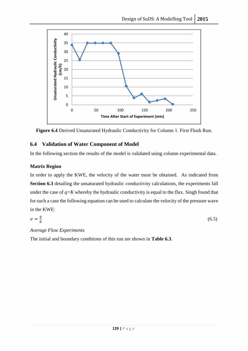
Design of SuDS: A Modelling Tool 2015
129 | P a g e
Figure 6.4 Derived Unsaturated Hydraulic Conductivity for Column 1. First Flush Run.
6.4 Validation of Water Component of Model
In the following section the results of the model is validated using column experimental data.
Matrix Region
In order to apply the KWE, the velocity of the water must be obtained. As indicated from
Section 6.3 detailing the unsaturated hydraulic conductivity calculations, the experiments fall
under the case of q=K whereby the hydraulic conductivity is equal to the flux. Singh found that
for such a case the following equation can be used to calculate the velocity of the pressure wave
in the KWE:
𝑣 =𝑞
𝜃 (6.5)
Average Flow Experiments
The initial and boundary conditions of this run are shown in Table 6.3.
0
5
10
15
20
25
30
35
40
0 50 100 150 200 250
Un
satu
rate
d H
ydra
ulic
Co
nd
uct
ivit
y (c
m/h
)
Time After Start of Experiment (min)

Design of SuDS: A Modelling Tool 2015
130 | P a g e
Table 6.3 Initial and Boundary Conditions For Average Flow Experiment
Parameter Value
Upper Boundary Condition 12 cm/h (0.2 cm/min)
Lower Boundary Condition Free Flow
Duration of Experiment 300 min
Initial Conditions Soil Moisture Content
(m3/m3)
Water Head (cm)
15 cm (Soil/Sand Upper Layer) 0.135 -45.1
55 cm (Soil/Sand Upper Layer) 0.193 -31.0
75 cm (Sand Lower Layer) 0.026 -26.0
Below a comparison of the results of the experiment and KWE for soil moisture content at
z=15 cm (soil) (Figure 6.5), 55 cm (soil) (Figure 6.6) and 75 cm (sand) (Figure 6.7) is shown.
Soil moisture is illustrated instead of water head as this parameter has been shown to have an
effect on heavy metal retention (Section 4.4.4.4). The van Genuchten parameters used are
detailed in Table 6.1 (soil/sand mix) and Table 6.2 (sand). The saturated hydraulic
conductivity (Ks) was taken as 77 cm/h for the upper soil/sand mix and 110 cm/h for the lower
sand layer (see Table 5.3).
The KWE was solved using the Thomas algorithm described in Appendix B1 and implemented
in Matlab.

Design of SuDS: A Modelling Tool 2015
131 | P a g e
Figure 6.5 Comparison of Experimental Soil Moisture Content at z=15cm with Kinematic
Wave Equation for Average Flow Condition
Figure 6.6 Comparison of Experimental Soil Moisture Content at z=55cm with Kinematic
Wave Equation for Average Flow Condition
0
0.05
0.1
0.15
0.2
0.25
0.3
0.35
0.4
0 100 200 300 400 500 600
Soil
Mo
istu
re C
on
ten
t (m
3 /m
3 )
Time After Start of Experiment (min)
Experiment
KWE
0
0.05
0.1
0.15
0.2
0.25
0.3
0.35
0 100 200 300 400 500 600
Soil
Mo
istu
re C
on
ten
t (m
3 /m
3)
Time After Start of Experiment (min)
Experiment
KWE

Design of SuDS: A Modelling Tool 2015
132 | P a g e
Figure 6.7 Comparison of Experimental Soil Moisture Content at z=75cm with Kinematic
Wave Equation for Average Flow Condition
As can be seen from Figure 6.5 and Figure 6.6 the KWE captures the overall movement of
soil moisture through the column well with R2=0.92 and a Nash-Sutcliffe coefficient = 0.91 for
z=15 cm and R2=0.86 and a Nash-Sutcliffe coefficient = 0.86 for z=55 cm. However there are
some minor inaccuracies in the drainage wave, this is due the steep drainage front characteristic
of kinematic wave approximations (Singh, 1997). This minor inaccuracy should not
significantly affect heavy metal retention as it only has a slight influence on relevant variables
(soil moisture content and pore water velocity) as illustrated in Section 4.4.4.4 .
For z=75cm the accuracy is given by R2=0.92 and a Nash-Sutcliffe coefficient = 0.87, the small
error is attached to the inaccuracy in the drainage wave which is overestimated by KWE. This
is attributed to the very high hydraulic conductivity in the sand layer (110 cm/h) compared with
the slower upper layer of compost/sand (77 cm/h) which, causes the discrepancy in velocity
between layers. In addition, the KWE diverges more during the drying phase as capillary action
is the dominant process, whereas with the KWE, gravity is the dominant mechanism of water
movement.
As is illustrated in Appendix D2, the hydrological results did not vary between the average
runs therefore a validation comparison for only one run is illustrated.
First Flush Experiments
The initial and boundary conditions of this run are shown in Table 6.4.
0
0.01
0.02
0.03
0.04
0.05
0.06
0.07
0.08
0.09
0 100 200 300 400 500 600
Soil
Mo
istu
re C
on
ten
t (m
3 /m
3 )
Time After Start of Experiment (min)
Experiment
KWE

Design of SuDS: A Modelling Tool 2015
133 | P a g e
Table 6.4 Initial and Boundary Conditions for First Flush Experiment
Experimental Setup
Upper Boundary Condition 35 cm/h (.583cm/min)
Lower Boundary Condition Free Flow
Duration of Experiment 90 min
Initial Conditions Soil Moisture Content
(m3/m3)
Water Head (cm)
15cm (Soil/Sand Upper Layer) 0.136 -44.75
55cm (Soil/Sand Upper Layer) 0.201 -31.3
75cm (Sand Lower Layer) 0.025 -26
Below a comparison of the results of the experiment and KWE for soil moisture content at
z=15 cm (soil) (Figure 6.8), 55 cm (soil) (Figure 6.9) and 75 cm (sand) (Figure 6.10) is shown.
Figure 6.8 Comparison of Experimental Soil Moisture Content at z=10cm with Kinematic
Wave Equation for First Flush Flow Condition
0
0.05
0.1
0.15
0.2
0.25
0.3
0.35
0.4
0 50 100 150 200 250 300
Soil
Mo
istu
re C
on
ten
t (m
3 /m
3)
Time After Start of Experimental (min)
Experiment
KWE

Design of SuDS: A Modelling Tool 2015
134 | P a g e
Figure 6.9 Comparison of Experimental Soil Moisture Content at z=55cm with Kinematic
Wave Equation for First Flush Flow Condition
Figure 6.10 Comparison of Experimental Soil Moisture Content at z=75cm with Kinematic
Wave Equation for First Flow Condition
Overall the KWE captures the overall movement of soil moisture through the column well with
R2=0.99 and a Nash-Sutcliffe coefficient = 0.98 for z=15 cm, R2=0.96 and a Nash-Sutcliffe
coefficient = 0.96 for z=55 cm and R2=0.86 and a Nash-Sutcliffe coefficient = 0.85 for z=75
cm. It is clear that the KWE accurately models soil moisture movement at the top of the column
but the accuracy decreases with depth. This is evident from the case of z=75 cm where the
KWE accurately models the wetting, however the prediction for the drainage wave has a very
0
0.05
0.1
0.15
0.2
0.25
0.3
0.35
0.4
0 50 100 150 200 250 300
Soil
Mo
istu
re C
on
ten
t (m
3 /m
3 )
Time After Start of Experiment (min)
Experiment
KWE
0
0.01
0.02
0.03
0.04
0.05
0.06
0.07
0.08
0.09
0.1
0 50 100 150 200 250 300
Soil
Mo
istu
re C
on
ten
t (m
3 /m
3 )
Time After Start of Experimental (min)
Experiment
KWE

Design of SuDS: A Modelling Tool 2015
135 | P a g e
sharp wetting front compared to the experimental results. This may indicate that diffusion is
not being properly quantified, this is an area for future work. This problem could potentially
be solved by incorporating an additional diffusion term into the KWE however it has been
shown that the KWE is accurate without this addition and it is deemed unnecessary at this time.
Macropore Region
As detailed in the previous chapter (Section 5.4.2), no macropore flow was observed with the
results of the tracer, breakthrough times and soil moisture content. Thus, one of the major
drawbacks of these experiments were their inability to validate the macropore section of this
model with experimental results. However, a detailed validation was completed in Section
4.4.2, this was deemed appropriate as the KWE displayed accuracy at predicting macropore
flow (R2>0.89) for four cases with different inflow rates and parameters proving its
applicability under a wide range of conditions.
6.5 Heavy Metal Retention Validation
As is clear from the previous chapter, breakthrough of the columns was not achieved therefore
the results for the linear distribution coefficient were obtained from very similar soils in the
literature (Table 6.5).
Table 6.5 Linear Distribution Coefficients for Experimental Substrates
Material Linear Distribution Coefficient (Kd) (L/kg) Reference
Cu Pb Zn
Soil/Sand
Upper Layer
4799 171214 11615 (Li & Davis
2008)
Sand
Lower Layer
1060 1295 1500 (Christensen et
al. 1996,
The figures below show a comparison between the experimental and linear isotherm results for
Cu (Figure 6.11), Pb (Figure 6.12) and Zn (Figure 6.13).
The results are shown for Column 3 as this was the column with the lowest retention.

Design of SuDS: A Modelling Tool 2015
136 | P a g e
Figure 6.11 Comparison of Linear Isotherm with Experimental Results for Cu.
Figure 6.12 Comparison of Linear Isotherm with Experimental Results for Pb.
99
99.5
100
100.5
101
101.5
102
0 1000 2000 3000 4000
% C
u R
ete
nti
on
Accumulated Experimental Time (min)
Experiment
Linear Isotherm
99
99.5
100
100.5
101
101.5
102
0 1000 2000 3000 4000
% P
b R
ete
nti
on
Accumulated Experimental Time (min)
Experiment
Linear Isotherm
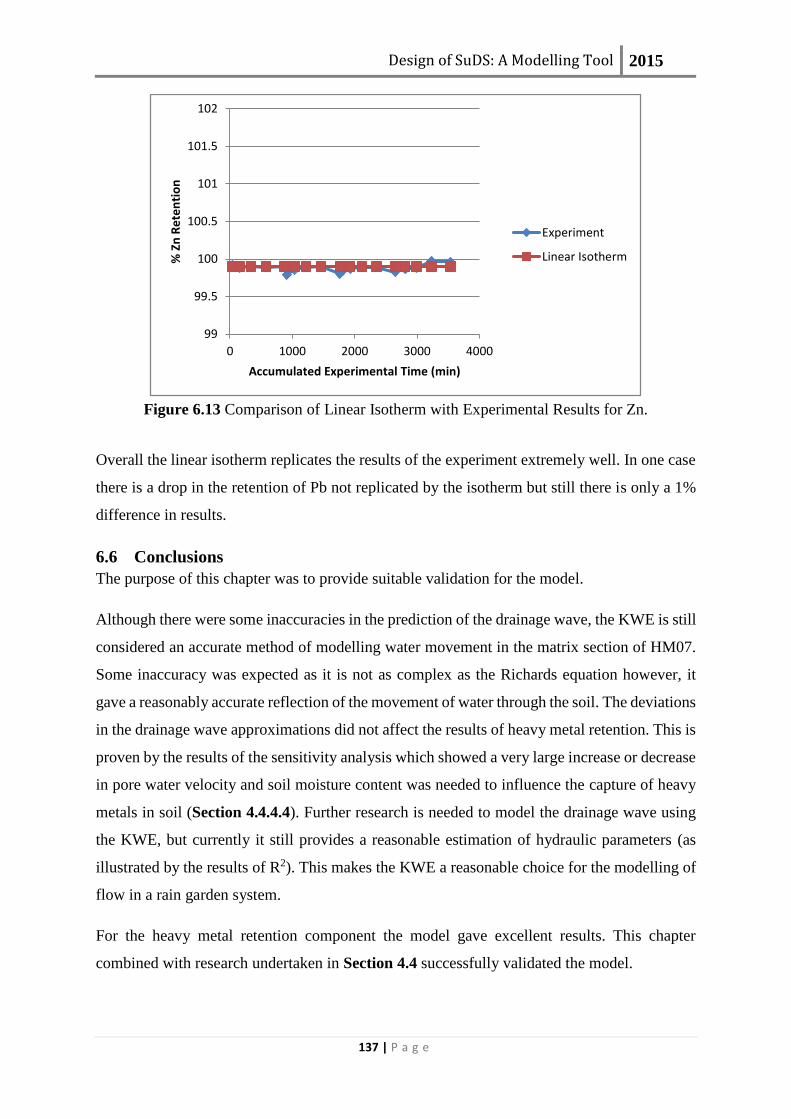
Design of SuDS: A Modelling Tool 2015
137 | P a g e
Figure 6.13 Comparison of Linear Isotherm with Experimental Results for Zn.
Overall the linear isotherm replicates the results of the experiment extremely well. In one case
there is a drop in the retention of Pb not replicated by the isotherm but still there is only a 1%
difference in results.
6.6 Conclusions
The purpose of this chapter was to provide suitable validation for the model.
Although there were some inaccuracies in the prediction of the drainage wave, the KWE is still
considered an accurate method of modelling water movement in the matrix section of HM07.
Some inaccuracy was expected as it is not as complex as the Richards equation however, it
gave a reasonably accurate reflection of the movement of water through the soil. The deviations
in the drainage wave approximations did not affect the results of heavy metal retention. This is
proven by the results of the sensitivity analysis which showed a very large increase or decrease
in pore water velocity and soil moisture content was needed to influence the capture of heavy
metals in soil (Section 4.4.4.4). Further research is needed to model the drainage wave using
the KWE, but currently it still provides a reasonable estimation of hydraulic parameters (as
illustrated by the results of R2). This makes the KWE a reasonable choice for the modelling of
flow in a rain garden system.
For the heavy metal retention component the model gave excellent results. This chapter
combined with research undertaken in Section 4.4 successfully validated the model.
99
99.5
100
100.5
101
101.5
102
0 1000 2000 3000 4000
% Z
n R
ete
nti
on
Accumulated Experimental Time (min)
Experiment
Linear Isotherm

Design of SuDS: A Modelling Tool 2015
138 | P a g e
7 MODEL APPLICATION 7.1 Introduction
In this chapter, HM07 was applied to the design of a rain garden facility located on a
roundabout in Thanet, Kent as shown in Figure 7.1. The existing and the proposed site layout
are shown in Figure 7.2 and Figure 7.3 respectively. The objective of this modelling exercise
was to not only examine the impact of different parameters on heavy metal retention in the
facility but also demonstrate the utility of the model for the design of such systems. The heavy
metals examined in this chapter are Cu2+ and Pb2+ as stated in Section 3.5 these are the most
common ionic composition of metals in storm water runoff.
Figure 7.1 Site Location Plan of Rain Garden

Design of SuDS: A Modelling Tool 2015
139 | P a g e
Figure 7.2 Existing Site Layout

Design of SuDS: A Modelling Tool 2015
140 | P a g e
Figure 7.3 Proposed Site Layout
7.2 Site Description
The rain garden was to be constructed on a roundabout in Thanet, Kent in the U.K. and receive
drainage from the road surrounding it. It was necessary to evaluate the potential pollutant
retention of the rain garden at this site as shallow groundwater was present. A preliminary
estimation of heavy metal retention in the rain garden using HM07 was viewed as the best
method of achieving this and as an efficient and simple tool for informing discussion between
Kent Council and the Environment Agency.
Several boreholes and detailed studies were completed by Pam Brown Associates. This allowed
for a relatively good characterisation of the subsoil which is a required model parameter. The
boreholes indicated an upper layer of made ground consisting of silty clay to 0.4 m and sandy
gravel underlying to 1.8 m (Pam Brown Associates, 2012). Groundwater was not encountered
directly at the site however it was found that in the vicinity (100 m away) saturated chalk lay

Design of SuDS: A Modelling Tool 2015
141 | P a g e
just 1.5 m deep (Pam Brown Associates, 2012). The upper layer was heterogeneous as it
consisted of several layers of made ground, however the lower layers of chalk were
homogeneous. It was noted that there was a possibility of soluble rocks at the site as indicated
by the British Geographical Society (http://www.bgs.ac.uk/products/geosure/soluble.html). It
would thus be prudent to complete further site investigation to ensure the rain garden did not
contribute to dissolution or degradation of the bedrock.
Table 7.1 Hydraulic Parameters of the Rain Garden
Soil Characteristic Root Zone Storage Zone Layer
Texture Loam Sand
Depth (cm) 30 30
Saturated Soil Moisture
Content (θsat) (cm3/cm3)
0.41 0.41
Residual Soil Moisture
Content (θres) (cm3/cm3)
0.02 0.041
Saturated Hydraulic
Conductivity (Ksat) (cm/h)
10.16 15
Figure 7.4 Diagram of Rain Garden Device

Design of SuDS: A Modelling Tool 2015
142 | P a g e
Hydraulic parameters common to rain garden soils were obtained from Dussaillant (2002) and
are provided in Table 7.1. a diagram of the device is shown by Figure 7.4. The depression
depth was set at 15 cm in agreement with previous rain garden design (Dussaillant, 2002)
The Ksat of the subsoil was 2 cm/h and was given by a soakaway test; further details are
available in the site report (Pam Brown Associates, 2012). Two distinct scenarios were
modelled, firstly the transfer and accumulation of heavy metals without macropore flow and
secondly, possible groundwater pollution caused by macropores.
A simulation period of ten years was chosen as it was deemed to give an appropriate measure
of time at which comprehensive maintenance may be expected. The rainfall data was given by
a local weather station at Manston (as shown Figure 7.1) approximately three miles from the
proposed site
(http://badc.nerc.ac.uk/cgibin/midas_stations/station_details.cgi.py?id=775&db=midas_statio
ns) and obtained from the British Atmospheric Data Centre
(http://badc.nerc.ac.uk/view/badc.nerc.ac.uk__ATOM__dataent_ukmo-midas). The interval
of 2003-2012 was chosen as it gave a sufficiently long period and included dry (2005) and wet
(2009) years. The Pb2+ input concentration was specified as 0.08 mg/L and corresponds to the
suggested level of synthetic runoff for rain garden design provided in Davis et al. (2001), it
also matches Pb2+ values found in runoff from a busy highway (M25 London orbital road
approximately 120000 vehicles per day) measured by Hares and Ward (1999). The Cu2+ input
concentration of 0.08 mg/L was also consistent with synthetic runoff values; this was double
the observed value experienced at roadside sites (Legret & Pagotto, 1999). Only Cu2+ and Pb2+
were examined in this study as they are most likely to pose a contamination risk, Pb2+ due to
accumulation and Cu2+ due to transfer through the system. Zn2+ was not examined as it does
not pose a significant risk of groundwater contamination or health risk (Li & Davis, 2008).
7.3 Accumulation and Transfer without Macropores
In this section, the accumulation of Pb2+ in the proposed rain garden was evaluated for two
upper layer soil substrates; an organically enriched soil (high retentive capacity) commonly
used in rain gardens and standard topsoil (low retentive capacity) (Davis et al. 2001, Li & Davis
2008). This was reflected in the linear distribution coefficient (Kd) values shown in Table 7.2.

Design of SuDS: A Modelling Tool 2015
143 | P a g e
Table 7.2 Heavy Metal Retention Parameters of the Soil
Soil Linear Distribution Coefficient (Kd) (L/kg) Reference
Pb2+ Cu2+
High
Retention
(Organically-
enriched)
Low
Retention
(Standard
topsoil)
High
Retention
(Organically-
enriched)
Low
Retention
(Standard
topsoil)
Loam 171214 500 4799 550 (Davis et al.
2001, Li & Davis
2008)
Sand 1295 1060 (Christensen et al.
1996)
Area ratios (see Section 2.6) were also considered in order to optimally design the device and
decrease the frequency of upper layer removal. Pb2+ was chosen as the focus as it was the only
metal known to exceed safety levels in rain garden soil (Li & Davis, 2008). Cu2+ behaviour
was also examined as it is the most likely heavy metal to cause groundwater pollution given its
high mobility in soil, even with no macropores present, and the fact that it was found not to
sorb as easily to soil as Pb2+ or Zn2+ (Li & Davis, 2008). The Kd values for Pb2+ and Cu2+ of
standard topsoil were similar (500 L/kg and 550 L/kg respectively), however for organically
enriched soil, the Kd value for Pb2+ is significantly greater than Cu2+ (171214 L/kg in
comparison with 4799 L/kg). This indicates that Pb2+ will sorb to the organic soil at a much
higher level than Cu2+.
The accumulation of Cu2+ in soil does occur but does not pose a health hazard and thus is not
examined for this device (Li & Davis, 2008).
7.4 Macropore flow
Typically macropores only occur in the root zone as this layer has the highest biological
activity. The storage zone is designed to be coarse sand or gravel, without organic matter, to
encourage flow and storage which makes it relatively inert and discourages growth of roots,

Design of SuDS: A Modelling Tool 2015
144 | P a g e
earthworm movement and other activities which increase macropore flow. However as
groundwater contamination was the key concern, the worst case scenario of a macropore
reaching 1.5m (depth of the groundwater) was examined. In previous studies, macropores have
been found to extend to this depth in soils similar to rain garden (Mallants et al., 1997). This
formation may take several years of development thus it is assumed that the macropore is active
for only a 7 year period compared to the total period of 10 years examined. The macropore
also received the maximum inflow possible. The model used the KWE to calculate macropore
flow rate, however the maximum flow rate in this case was limited to 2 cm/h owing to the
maximum infiltration rate of the lower layer of chalk. This infiltration rate was measured using
a soakaway test during the initial site investigation (Pam Brown Associates 2012).
7.5 Results
7.5.1 Matrix Flow
Using HM07 and the parameters discussed above, results for Pb2+ concentration in the upper 5
cm of the rain garden after a period of 10 years with an area ratio (AR) of 5 and 10%
respectively and highly retentive soil are shown in Figure 7.5. The maximum concentration in
the rain garden with AR=10% was 568 mg/kg. However if the area ratio was decreased to 5%
to minimise construction costs, the level of Pb2+ accumulation increased significantly to 1209
mg/kg, higher than the allowable Pb2+ concentration in soil of 750 mg/kg (Pam Brown
Associates, 2012) . This limit was set for industrial land use by the Environment Agency (Pam
Brown Associates, 2012).

Design of SuDS: A Modelling Tool 2015
145 | P a g e
Figure 7.5 Pb2+ Concentration in Rain Garden Soil with Highly Retentive (Organically-
Enriched) Soil (Kd=171214 L/kg) and Lower Retentive (Standard) Topsoil (Kd=500 L/kg)
and Two Area Ratios.
For soil with a lower Kd value, the accumulation in the upper layer of the systems for both area
ratios is reduced as illustrated in Figure 7.5b.
In addition to accumulation in the system, it is important also to consider the possibility of
groundwater pollution caused by this lower retention. Figure 7.6 shows the simulation results
for Pb2+ concentration in soil-water for a lower Pb2+ retention rate in the upper layer after a
period of 10 years. It indicates that in the case of an area ratio of 5%, Pb2+ does not reach a
depth of lower than 43 cm much lower than the total depth of 60 cm, thus Pb2+ was retained in
the device.

Design of SuDS: A Modelling Tool 2015
146 | P a g e
Figure 7.6 Pb2+ Concentration in Water for Lower Retentive Topsoil with a 5% Area Ratio
after 10 years.
For the case of Cu2+, Figure 7.7 illustrates results for concentration in soil-water through the
soil profile for highly retentive soil with an area ratio of 5 and 10% after 10 years. It shows that
Cu2+ soil-water concentration is negligible at 30 cm which indicates that all retention is taking
place in the upper layer. It also shows that area ratio has little effect on this concentration.
If however, the soil has a lower retention capacity such as normal topsoil (Table 7.2) it is
observed that the majority of retention after a 10 year period takes place in the lower storage
layer (Figure 7.8).

Design of SuDS: A Modelling Tool 2015
147 | P a g e
Figure 7.7 Cu2+ Concentration in Soil-Water for Highly Retentive (Organically Enriched)
Soil and Two Area Ratios after 10 Years.
Figure 7.8 Cu2+ Concentration in Water for High (Kd=4799 L/kg) and Lower Retentive
(Kd=550 L/kg) Soil with a 5% Area Ratio after 10 Years.

Design of SuDS: A Modelling Tool 2015
148 | P a g e
7.5.2 Macropore Flow
In this section, the effect of macropore flow on groundwater pollution is examined. Figure 7.9
shows the Cu2+ water concentration in a single macropore for soil with the higher retention
value after a period of ten years that has received the maximum water input based on the
limiting factors stated in Section 7.4. This figure illustrates that Cu2+ is removed from the
runoff in the root zone and that no groundwater pollution occurs due to macropore flow for
organically enriched soil.
Figure 7.9 Cu2+ Concentration in Macropore Water for Highly Retentive (Organically
Enriched) Soil and Two Area Ratios after 10 Years.
While Figure 7.10 shows the Cu2+ water concentration in macropore flow for topsoil, Cu2+ is
removed from the runoff by 55 cm depth for the worst case scenario (low retentive soil and an
area ratio of 5%).

Design of SuDS: A Modelling Tool 2015
149 | P a g e
Figure 7.10 Cu2+ Water Concentration in Macropore Water for Lower Retentive Topsoil and
Two Area Ratios.
7.5.3 Sensitivity Analysis
In order to quantify the effects of uncertainties in important parameter values, a sensitivity
analysis was performed. The focuses of this examination were the variables Kd, Ksat and A as
these have been shown to be the determining factor for retention. The reference values chosen
for this analysis are those used earlier which are listed in Table 7.1 and Table 7.2. As the main
concern of this examination was to prevent groundwater contamination at the site, the effects
of these variables on the Cu2+ outlet concentration in water from the upper layer of the system
were examined (Figure 7.11).
From the sensitivity analysis (Figure 7.11), a linear relationship between the outlet water
concentration and the value of Kd exists: this is to be expected as the linear isotherm is used.
Minor deviances from the reference value do not influence the results substantially, only when
the value of Kd is altered by above ±50% are major effects (±10%) on the Cu2+ outlet
concentration seen. The outlet concentration is most sensitive to the value of saturated
hydraulic conductivity Ksat. For low values of Ksat, outlet concentration is low, which may be
due to increased overflow from the system and/or decreased pore water velocity through the

Design of SuDS: A Modelling Tool 2015
150 | P a g e
soil. The analysis shows that varying the other parameters did not have a significant impact on
results.
A sensitivity analysis was not performed on macropore flow as the potential factors (number,
velocity and capacity of macropores) would not significantly affect the results for outlet
concentration given the maximum flow rate through the macropores of 2 cm/h determined by
the lower layer of chalk.
Figure 7.11 Sensitivity Analysis
7.6 Discussion
For highly retentive soils, the results for Pb2+ corresponded well to experimental findings by
Li and Davis (2008) in that the majority of Pb2+ retention was limited to the upper 10 cm of
soil (Figure 7.5a). The levels of accumulation were diminished when the value of Kd was
reduced (Figure 7.5b) and a more even distribution of lower Pb2+ accumulation through the
upper layer of the system was observed. Despite this, in all cases the rain garden demonstrated
excellent performance in Pb2+ removal and no groundwater contamination was predicted in the
10 year period examined (Figure 7.6). However, the risks posed by the accumulation of this

Design of SuDS: A Modelling Tool 2015
151 | P a g e
metal required additional investigation. As the roundabout was not accessible to the public, the
soil pollutant guidelines for industrial and commercial sites provided by the Environmental
Agency were appropriate; the regulatory level for Pb2+ in these guidelines is 750 mg/kg (Pam
Brown Associates 2012). This indicated that in the case of the lower area ratio (5%), the first
1 cm of soil needs to be replaced within the 10 year period examined after approximately 6
years. This would cause a large degree of inconvenience as it requires vegetation be removed.
The reason the contamination is limited to 1cm is due to the high adsorption capacity of the
soil for Pb2+ however this would not be the case in all circumstances. For example, if the Kd
was lower but still large enough to facilitate high rates of retention, a dangerous level of
accumulation would be distributed to a greater depth. For A=10% the level of accumulation did
not exceed regulatory guidelines provided by the Environmental Agency therefore no action
needed to be taken.
If this rain garden was situated in a residential area, the maximum allowable concentration
decreases to 350 mg/kg due to the possibility of human contact and thus would require remedial
action at more regular intervals even with an area ratio of 10% .This highlights the need to
design rain gardens on an individual basis and further underlines the utility of this model.
With regards to Cu2+, again substantial retention was predicted, also in line with experimental
evidence (Davis et al. 2001). Results shown in Figure 7.7 indicate that the water concentration
values were minimally affected by a decreased area ratio. A possible reason for this is that a
large increase in pore water velocity is required to have an effect on retention, an aspect which
needs to be further investigated. The majority of rainfall events at the site are of lower
precipitation values (<10mm) thus a significant rise in velocity is only seen during exceptional
events minimally affecting retention.
When the Kd value of the upper layer is reduced, the majority of Cu2+ capture shifts to the
storage zone, but no metal flux is predicted from the rain garden to the subsoil and groundwater
(Figure 7.8). It is thus, beneficial for the lower storage layer to also have high Kd values to
ensure that despite metal flux from the upper layer no pollution reaches the subsoil.
In the case of macropore flow, no Cu2+ flux is predicted to enter groundwater (Figure 7.9 and
Figure 7.10). This is caused by the limiting infiltration rate of the chalk of 2 cm/h (see Section
7.4) which decreases the maximum velocity in the macropore and thus increases sorption,
sorption does not typically occur in the macropores as their water velocity can be in excess of
134 cm/h (Jury & Horton, 2004). It is therefore important to consider each situation

Design of SuDS: A Modelling Tool 2015
152 | P a g e
individually. Overall, these observations emphasize the relevance of this recently developed
model, particularly given that macropores are not considered in the proposed standards for
SuDS design (DEFRA, 2011).
In summary, the model results imply that a higher distribution coefficient coupled with a low
area ratio results in large levels of Pb2+ accumulation. Thus, in order to evenly distribute Pb2+
throughout the upper layer of the rain garden, soils with lower Pb2+ distribution coefficient may
be more efficient. This would reduce the need for frequent costly removal of contaminated
soil. Macropore flow did not affect groundwater quality given the limiting infiltration effect of
the lower layer of chalk. Therefore, in this particular case, an area ratio of 5% is recommended
to decrease construction and maintenance costs. A soil with a lower Kd value can be used for
the upper layer to prevent hazardous metal accumulation, but care should be taken to ensure
the storage layer has enough retention capacity itself to offset the decreased heavy metal
retention this would cause.
It is clear from the findings of this examination that it is of vital importance to monitor the fate
of heavy metals in SuDS during the design process, to ensure the creation of an optimum
device. The advantages of the developed model over conventional design techniques such as
standards (DEFRA, 2011) are also illustrated as it allows for rain gardens to be individually
assessed based on their specific situations including climate change, soil conditions and design
parameter sets. This can be achieved by running simulations and varying the soil type, layer
depth, area ratio and rainfall levels enabling a detailed examination of these different situations
and their impact on groundwater recharge and heavy metal retention.
Finally, the model allows for the examination of possible consequences of choosing a design
with decreased construction costs such as a low area ratio which could lead to increased
overflow and need for increased maintenance. It can also be used to develop maintenance
schedules. This can be achieved by running simulations before construction whereby an
indication of when Pb2+ accumulations reach regulatory limits can be found. These findings
can be updated whenever further information is gathered, such as heavy metal runoff
concentrations.
In its current state however the model does not simulate the behaviour of other pollutants such
as nutrients and hydrocarbons which are also of concern, but the isotherms for these pollutants
can be added to this model in the future.

Design of SuDS: A Modelling Tool 2015
153 | P a g e
8 DISCUSSION 8.1 Introduction
In this chapter a discussion is given which addresses all aspects pertinent to the proposed
model. Firstly, the issue of applicability and purpose will be examined, starting with the
models use as a research and design tool for rain gardens and how it compliments current
research. Its applicability to other infiltration based SuDS (green roofs) is then examined, along
with any adaption which will need to be made.
Secondly, the advantages and limitations of the model are discussed in the context of other
options available for the prediction of heavy metal retention in rain garden systems.
Finally, the main contributions of knowledge that this thesis provides are detailed and
discussed.
8.2 Application of the Model
8.2.1 Rain Gardens
As discussed in Chapter 7, this model can be used to provide an accurate method of predicting
heavy metal retention and accumulation in rain gardens over long periods of time.
Currently, there are few studies completed into the long term heavy metal removal capacity of
these systems. Paus et al. (2014) examined the saturated hydraulic conductivity (Ksat) and
heavy metal accumulation of three rain gardens over a period of four years. They found that
the Ksat increased by between 300 and 600%. This, coupled with a decrease in bulk density of
between 10-22%, indicates macropore flow, although this is never identified in the paper.
Unfortunately, the metal accumulation is only measured at the end of the four year period so a
direct correlation cannot be established between macropore flow and a decrease in retention.
However, it was found that the Cd and Zn concentrations were lower than the estimated
sorption capacities for the media which could be due to bypass of the matrix regions by
preferential flow. It was stated by the authors that there is a need to investigate a wider range
of rain gardens to establish the key factors effecting long term infiltration and retention
performance. This need could partially met by utilising the fully validated model to examine
scenarios including changes of Ksat with time and possible macropore flow.
Current research is focussing predominantly on the examination of possible media and their
effects on hydraulic conductivity and retention removal (Paus et al. 2014, Jones & Davis,

Design of SuDS: A Modelling Tool 2015
154 | P a g e
2013). In the future, the model in this thesis could complement this research by utilising the
findings and running simulations which examine the effect of parameter variation. Thus this
model provides an excellent addition to research in the field of pollutant retention in SuDS.
8.2.2 Green Roofs
Green roofs are another type of infiltration based SuDS. The general construction of a green
roof consists of four layers: vegetation layer, soil layer, filter and drainage material (Czemial
Berndtsson, 2010). They are generally separated into two main classes: intensive, typified by
deep layers of soil which can support larger flora and extensive, which are characterised by
very thin soil layers and large coverage areas. Obviously the main aim of a green roof is
different to a rain garden in that it does not increase groundwater recharge but seeks to diminish
the peak storm flow (through soil retention) which can cause flash flooding and disruption in
cities. It is still important to ensure heavy metals are retained by these systems so that when the
delayed runoff reaches either sustainable or conventional drainage systems environmental
contamination does not occur. An example of maximum and minimum heavy metal
concentrations in urban runoff is given in Table 8.1 (Gobel et al., 2007).
Table 8.1 Heavy Metal Concentrations in Rainfall
Heavy Metal
Concentration
(μg/L)
Rainfall
Min Max
Cu 1 355
Pb 2 76
Zn 5 235
Green roofs share many similar characteristics to rain gardens such as layered soil profiles and
vegetation however there are some unique differences most notably slope and drainage method
(as green roofs do not drain into subsoil, their runoff is directed to outflow pipes). It has been
found that slope does not influence the shape of the direct runoff hydrograph however it does
impact water retention within the green roof: the lower the slope the higher the retention this
is due to the decreased infiltration capacity of slopes (Getter, et al., 2007). The kinematic wave
equation is commonly used to model unsaturated subsurface flow on hillslopes (Beven, 1982;
Singh, 1997; Norbiato & Borga, 2008); therefore it should be easy to adapt the model to suit a

Design of SuDS: A Modelling Tool 2015
155 | P a g e
green roof. In addition a simple reservoir routing equation similar to that used by She and Pang
(2010) can be incorporated to model the drainage from the device.
There are several computer models which have been used to examine the hydrological
performance of green roofs, some have been developed specifically for this purpose (She &
Pang, 2010) and others such as HYDRUS (Hilten, et al., 2008) and SWAP (Metselaar, 2012)
have been adapted with mixed results. However to the author’s knowledge a model has never
been used to examine heavy metal retention or pollutant transfer through macropores in these
systems.
With regards to metal retention, it has been observed that green roof runoff typically reduces
the loads of heavy metals in rainfall and runoff. However some metals appear in green roof
runoff in concentrations that would correspond to moderately polluted water (Czemial
Berndtsson, 2010). For example, a monitored extensive green roof in Sweden Cu outflow was
increased fourfold and only 8% of Zn retained. This supports the work of Gnecco et al. (2013)
who found that the use of certain substrates can lead green roofs to become a source of heavy
metal contamination. This again has been observed in aging green roof such as the 43 year old
intensive green roof at the University of Manchester which has become a source of Pb pollution
(Speak, et al., 2014). Other green roofs display excellent retention of heavy metals such as the
semi extensive (99% retention of Pb, Zn and Cu) and extensive (99% Pb, 97% Cu, 96% Zn)
systems examined by Steusloff (1998).
Macropore flow has never been examined in the context of green roofs but it is of vital
importance to consider due to the shallow nature of these systems and could possible explain
the large variance in retention between green roofs. It has also been observed by Getter et al.
(2007) that over a period of five years, the pore space in an intensive roof increased from
41.41% to 81.84%, this increased water holding capacity but would surely have an impact on
metal retention; unfortunately this was not examined.
Another less common aspect of green roof research is their use for vegetable production owing
to predicted food shortages in the future (Whittinghill, et al. 2013). If the roofs become
contaminated with heavy metals this avenue will not be possible so it is important to take this
into account.

Design of SuDS: A Modelling Tool 2015
156 | P a g e
The findings above indicate that the behaviour of heavy metals in green roofs is a complex
subject dependent on a number of factors. Therefore the application of the discussed model to
this area would be a significant contribution to this field of research.
8.2.3 Permeable Pavements
Permeable pavements are an alternative to traditional impermeable asphalt and concrete
surfaces. Permeable pavements enable stormwater to either infiltrate into an underground
storage basin or soil resulting in groundwater recharge while also potentially removing
pollutants (Bean et al., 2007). Permeable pavement designs vary greatly although generally
they comprise of a series of layers as shown in Figure 8.1.
Figure 8.1 Diagram of a Permeable Pavement (Scholz & Grabowiecki, 2007)
This type of permeable pavement comprises of four distinct components:
paving slabs or bricks;
unsaturated zone of the base material;
saturated zone of the base material; and
sub-grade.
One of the key differences between permeable pavements and other SuDS such as rain gardens
and green roofs is the presence of a geotextile. Geotextiles are needed to prevent sand from
migrating through the layers, reduce rutting depth and retain and degrade oil and nutrients. In
terms of heavy metal retention, Legret et al. (1996) showed that suspended solids and lead can
be reduced by PPS up to 64% and 79%, respectively. Generally, PPS are efficient in trapping
dissolved heavy metals in surface runoff. However, not all pavers and joint fillings have the
ability to trap dissolved heavy metals. Pavements with large joints for infiltration must have a
suitable joint filling. Otherwise, metals will pass through them, and may subsequently enter
groundwater resources. Particles usually accumulate in geotextiles and on pavement surfaces.

Design of SuDS: A Modelling Tool 2015
157 | P a g e
Geotextiles usually separate micropollutants such as cadmium, zinc and copper from the
underlying soil, therefore preventing groundwater from becoming contaminated (Legret et al.,
1996)
HM07 can be used to predict both the movement of water and the retention of heavy metals in
a permeable pavement systems. The unsaturated and saturated zone and subgrade are all types
of material with known parameters and can be modelled as layers of soil HM07. The geotextile
material is more problematic. There are many types of geotextile material available however
their properties are well researched (Aydilek & Edil, 2004). The key parameters required for
modelling water transport are porosity and permittivity as detailed in Section 3.4 both of which
have been calculated for a variety of geotextiles (Aydilek & Edil, 2004).
For heavy metal retention, linear, Freundlich and Langmuir retention coefficient for the
geotextiles are required. These will need to be obtained via an experiment similar to that
completed by Davis et al. (2001).
8.3 Advantages of the Model
When developing this thesis, the aim was to find a balance between a competent, highly
accurate model that can be used for research, and an appropriate tool for design purposes
(simulating long input rainfall datasets).
Prior to this thesis, no specifically- designed model existed which could be used to predict the
extent to which heavy metals were captured in rain garden systems. As discussed in Appendix
A, HYDRUS is a software package for simulating water, heat, and solute movement in variably
saturated media. HYDRUS is generally used to model the water flow and solute transport and
then combined with a more complex geochemical speciation model (Jacques, et al., 2008) or
uniquely scaled sorption isotherm (Xiao, et al., 2013) to predict metal retention. In both cases,
the movement of heavy metals was accurately quantified, however HYDRUS was primarily
aimed as a research tool and is difficult to modify, is site specific and requires extensive
calibration.
In addition, HYDRUS has been found to require a long CPU time. It was found by Noranbuena-
Contreras at al. (2012) that a period of approximately 8 days was required to simulate rainfall
infiltration into an embankment with a fine mesh of 3848 nodes and 7457 triangular elements
in Hydrus 2-D. Typically HYDRUS 2-D takes three times as long as HYDRUS 1-D but this

Design of SuDS: A Modelling Tool 2015
158 | P a g e
still equates to computational time of almost 3 days which would be unacceptable to engineers
designing these facilities (PC-PROGRESS, 2012).
The combination of complexity and long computational times make the above option
inappropriate as a design tool. These issues are addressed by the model proposed by this thesis,
which currently uses a Matlab interface which simply requires the parameters of the rain garden
and precipitation values. For the case study in Chapter 7 it took approximately 4 hours to run
for each 10 year case, using hourly data. The model still retains accuracy as illustrated in
Section 4.4.1 whereby it successfully replicated the results of the Richards’ equation with an
R2=0.993.
8.4 Limitations
The current study only focused on one of the major pollutant groups present in urban storm
water, heavy metals (in particular Cu and Pb); thus the other pollutant groups, hydrocarbons
and nutrients are not taken into account. The model however includes hydraulic characteristics
which impact all the contaminant groups so in the future it is possible to add further subroutines
which include the other contaminants (see Section 9.3).
Another factor that became apparent in testing is the kinematic wave equations’ inability to
fully quantify diffusion occurring during drainage as shown in Section 6.4. However the minor
influence this inaccuracy has on soil moisture content and pore water velocity does not
significantly affect heavy metal retention prediction as illustrated in Section 4.4.4.4. More
importantly, KWE diverges more from Richards equation when soil gets drier
(suction>gravity), but in a rain garden context the soil is encouraged to be perpetually
inundated with water from the surrounding area so aridness is rare.
8.5 Contribution to Knowledge
Throughout this project there have been several key contributions to knowledge. These are
split into three key sections Model, Experimental and Simulation
8.5.1 Model
As stated numerous times in this thesis, HM07 was created to predict heavy metal retention in
a rain garden facility. This model can be used for research (to examine the key factors which
make a high performance rain garden system) and also to design these devices (Quinn &
Dussaillant, 2014). No other model similar to this existed previously and this is deemed to be
a unique contribution to research.

Design of SuDS: A Modelling Tool 2015
159 | P a g e
8.5.2 Experimental
The experiment detailed in this thesis was the first to examine the effect of macropores on
heavy metal retention in a sustainable drainage system. As discussed in Section 3.2 macropore
flow is a key factor in the capture of pollutants so these experiments are a crucial next step in
the research area of pollutant retention in rain gardens. The outflow of these systems was
analysed with a very low level of detection: 0.03 μg/L for Cu, 0.01 μg/L for Pb and 0.1 μg/L
for Zn with only 5% error, this allows for highly accurate results and the analysis of minute
difference between matrix and macropore columns. As discussed in Section 5.5.1, it was found
that hydraulically there was no difference between matrix and macropore columns possibly
owing to speed restrictions in macropores or the assertion in Section 4.2.2.3 that water transfer
between macropore and matrix soils is instantaneous in rain garden soil. The column soil was
also of a much higher permeability than that recommended for a rain garden. Despite this
finding, macropore flow still has a minor influence on Cu retention, decreasing in macropore
columns, this indicates that macropores still have an influence on heavy metal retention and
this requires further research. This is a significant finding as it indicates that even for highly
permeable soils, macropore flow still facilitates heavy metal transport through the system.
8.5.3 Simulations
It was found during the simulations discussed in Chapter 7 that soils with high retention
capacity are not necessarily suited for rain gardens as they can lead to dangerous levels of
accumulation of Pb. This can be prevented by using a less retentive substrate while still
maintaining groundwater quality.
It was observed when undertaking the sensitivity analysis that area ratio and saturated hydraulic
conductivity did not significantly affect the retention of Cu. This had never previously been
simulated to the author’s knowledge.

Design of SuDS: A Modelling Tool 2015
160 | P a g e
9 CONCLUSION AND FURTHER
WORK 9.1 Introduction
This chapter examines the objectives provided in Section 1.3 and evaluates their progress.
Having completed this conclusion, future work is identified.
9.2 Conclusions
In order to provide a comprehensive set of conclusions for this thesis, this chapter has been
divided into sections which evaluate the findings of the research in terms of the contributions
they have made to the main objectives of this thesis.
With respect to Objective One (Investigate the key factors affecting pollutant retention
including both soil type and hydraulic functions and examine which equations best model the
effects of these influences on heavy metal retention):
An in-depth literature review (Chapter 3) was carried out which provided the necessary
background knowledge for this project in terms of understanding theory and the
implementation of equations (runoff pollutants, variably saturated flow through porous
media, dual-permeability models, solute transport and retention).
As part of this review heavy metals were chosen as the sole focus of the pollutant
retention model as they posed the greatest health hazard. In addition, the key factors
which affected their retention in rain gardens were identified. These were found to be
split into two distinct groups; hydrological and soil related (vegetation also affected
retention but to a much lesser extent). The hydrological factors largely revolved around
the pore water velocity with increased velocity resulting in decreased retention, soil
water content and the presence of macropore flow which can prevent a large amount of
retention by transferring the runoff directly through the rain garden. The soil
characteristics were dependent on properties such as bulk density and distribution
coefficients for various isotherms; it was also found that the organic matter content of
the soil had a beneficial impact on heavy metal capture providing that the soil is also
well graded.

Design of SuDS: A Modelling Tool 2015
161 | P a g e
With regards to water modelling, dual permeability models were examined and
methods of modelling flow in both the matrix and macropore regions. Determining the
initiation of macropore flow and transfer between the regions were discussed.
In terms of heavy metal retention, the accuracy and applicability of different isotherms
were assessed along with methods of solute transport prediction.
This objective was deemed to be complete as the relevant literature was consulted and
this provided a solid base from which a computer model could be designed.
With respect to Objective Two (Develop and verify a simple dual-permeability model
specifically designed to model both water flow and contaminant retention in a rain garden using
the findings from the above objectives and results from literature.):
It was decided to develop a dual-permeability approach to the water modelling section
so that both flows in the matrix and macropore regions could be accounted for. The
kinematic wave equation was chosen to model water movement in both regions as this
provides a simpler alternative to more complex methods such as the Richards equation
while still maintaining good accuracy. With regards to the heavy metal modelling three
isotherms were chosen: the linear, Langmuir and Freundlich equations, as these showed
the most promising results from literature data. All three were examined as they each
added beneficial attributes to the model; linear for initial estimations, Langmuir for
particles with little surface roughness and Freundlich for coarse particles. These
isotherms were incorporated into the one dimensional advection-dispersion-adsorption
equation so that both transport and retention could be modelled together. The equations
chosen and the reasoning behind these decision were discussed in Chapter 4.
A number of requirements were listed in Table 4.15 which needed to be met in order
to develop a useful pollutant retention model. It was found that the created model met
all of these requirements (Table 4.15).
This model was verified in three parts, the matrix, macropore and pollutant retention
sections (Section 4.4). The matrix portion was tested against cases which illustrated
situations common in rain garden systems, specifically sharp wetting fronts (Celia, et
al., 1990) and layered soil profiles (Pan & Wierenga, 1995) and showed excellent
results (Section 4.2.1). The macropore section was validated against experiments
completed by Mdaghri-Alaoui & Germann (1998). These cases were chosen as suitable

Design of SuDS: A Modelling Tool 2015
162 | P a g e
validation for the macropore segment of this model as the four runs examined were
performed on a layered soil and encompassed a large range of infiltration, conductance
and exponent values. The macropore section showed good agreement with the
experimental results (Section 4.4.2). The linear isotherm model was tested against the
experimental results of Davis et al. (2001) as these were performed with rain gardens
specifically in mind and again the results were good (Section 4.4.3)
The Langmuir and Freundlich isotherms were validated using data from the Highways
Research Group (2010) and were found to give accurate results. A sensitivity analysis
was also performed and it was found that only dramatic increases (velocity i.e. inflow
or saturated hydraulic conductivity (Ks)) or decreases (bulk density) had an effect on
the % of heavy metal retained. The other factors of dispersion coefficient and porosity
had no significant impact. This indicated that for the case of increases in velocity
caused by high inflow rates or high Ks and decreases in bulk density caused by
heterogeneity of the soil retention was not decreased dramatically (Section 4.4.4).
From the detailed model developed and the preliminary validation discussed in
Chapter 4, this objective was deemed to be complete.
With respect to Objective Three (Design and perform column experiments that both provide a
unique contribution to rain garden research but also serve to provide further validation of the
model routines):
This objective was achieved by analysing past experiments and identifying an area
where research is lacking; this area was the effect of a single artificial macropore on
heavy metal retention in a layered soil column (with similar soil layout to a rain garden)
under typical English climatic conditions. The findings of these experiments indicated
that although macropore flow did not impact the hydraulic performance of the columns,
retention of the most mobile heavy metal, Cu, decreased slightly by the presence of
macropores. This was attributed to macropore flow moving at the same speed as flow
in the matrix region due to its natural speed limit and the high permeability of the soil.
However retention in the macropores was less than the matrix region resulting in
increased outflow Cu concentration from those columns.
The overall heavy metal retention of the columns was high (>99%) proving that under
English climatic conditions macropores are not a dominant factor in either the

Design of SuDS: A Modelling Tool 2015
163 | P a g e
movement of water or pollutant through a rain garden. This finding supports the
presumptions previously made regarding macropore initiation and transfer.
Finally the results of the column experiments were compared to the prediction of the
model. Unfortunately, it was not possible to validate the macropore section due to
inconclusive results and the high hydraulic conductivity of the soil. The predictions of
the kinematic wave equation agreed well with the results from the matrix region
(R2>0.86). It was found that similar to the preliminary validation there were problems
quantifying the drainage wave although this would not significantly affect pollution
retention results (Section 6.4). Finally it was shown that there was good agreement
between the predicted heavy metal outflow by the linear isotherm and the column
results (Section 6.5).
From the experimental results (Chapter 5) and validation (Chapter 6) this objective
was deemed to have been met.
With respect to Objective Four (Perform simulations to examine effect on pollutant retention
of rain garden design parameters including surface area and soil choice):
In Chapter 7, the model was applied to the design of a rain garden system for a planned
roundabout in Kent, U.K. The preliminary design considered an upper root zone layer
with organic soil and a sandy storage sublayer each 30 cm thick, for a rain garden with
area ratio of 5 and 10%. One of the principle scenarios examined was the accumulation
and movement of metals without macropores. It was shown that levels of lead can build
up in the upper layers of the system and constitutes a health hazard (surpass
Environment Agency U.K. standard of 750 mg/Kg) after 10 years. Simulations showed
that Cu was successfully retained (no significant concentrations below 50 cm of rain
garden soil depth). Therefore in this case it was recommended that soil with a lower
retention capacity be used for the upper layer to prevent hazardous Pb accumulation,
but care should be taken to ensure the storage layer had enough retention capacity itself
to offset the decreased heavy metal retention this would cause. This finding is in
contrast to intuitive knowledge which suggests the use of specialist soil with a high
capacity for metal retention be used in these devices. Care should be taken however
when selecting soil with distribution coefficients based on batch and column studies.
As discussed in Section 4.4.4.3 the adsorption parameters for heavy metals followed
the order of batch>column>field. Thus it is proposed that a safety factor be applied to

Design of SuDS: A Modelling Tool 2015
164 | P a g e
parameters obtained from batch and column experiments in the future, or that sensitivity
analysis be completed to ensure that sufficient retention occurs even if the distribution
coefficient is significantly decreased.
With respect to Objective Six (Investigate the effects of different hydrological processes such
as macropore flow):
Rain garden soils have different characteristics from the agricultural clay soils which
are typically examined with regards to macropore flow; they have a high saturated
hydraulic conductivity and are not as prone to cracking at the soil surface. They
therefore require different approaches and equations to model preferential flow. Rain
garden soils typically have higher infiltration rates and a finer consistency which results
in a very high hydraulic conductivity, this facilitates easy transfer from the macropore
to matrix region (Section 4.2.2.3). Therefore a water transfer term is often not needed
as the worst case scenario (no transfer of water) only occurs when the rain garden is
saturated when no transfer is possible. This is often not the case in agricultural soils
(modelled by HYDRUS, MACRO and RZWQM) whose consistency often causes
ponding before saturation.
The column experiments further supported this argument: they indicated that
macropore flow travelled at the same velocity as matrix flow or possibly was transferred
into the matrix region. The outflow concentration of Pb and Zn was unaffected by the
macropores present. Cu showed an increase in outflow concentration from the
macropore columns indicating that macropore flow does affect the retention of the most
mobile of heavy metals. A detailed discussion of these issues is available in Chapter
5.
Finally with regards to the simulations completed in Chapter 7 macropore flow was
examined by the model for a case where groundwater contamination was a possibility
due to preferential flow bypassing the retention capabilities of a rain garden. Results
indicated that, due to site conditions macropore flow was not a threat to groundwater at
this location for the time frame considered. In addition, a sensitivity analysis was
completed to examine the effects of other parameter: saturated hydraulic conductivity
(Ksat), area ratio and distribution coefficient. The outlet concentration is most sensitive
to the value of saturated hydraulic conductivity Ksat. For low values of Ksat, outlet
concentration was low, which may be due to increased overflow from the system and/or

Design of SuDS: A Modelling Tool 2015
165 | P a g e
decreased pore water velocity through the soil. The analysis showed that varying the
other parameters did not have a significant impact on results. The results are detailed in
Chapter 7 and this objective was deemed to be met.
Further sensitivity analysis was carried out to examine the hydrological parameters
related to retention predicted by the Freundlich isotherm (Section 4.4.4.4). It was found
that pore water velocity had a minimal effect on retention whereas porosity (soil
moisture content) and diffusion were negligible. This supported the use of less complex
equations such as the kinematic wave equation which gave accurate results but was less
precise than the more complex Richards equation which required more computational
power.
9.3 Further Work and Recommendations
It is suggested that further work on this project address the limitations discussed in Section 8.4.
This would begin by expanding the model to include hydrocarbons and nutrients possibly using
the methods outlined in Table 3.1. The priority would be hydrocarbons as these have been
identified by the Highways Agency as significantly damaging to the natural environment
(Highways Research Group, 2010). The movement of hydrocarbons through soil is often
comprised of a three-fluid phase system with air, water, and a nonaqueous phase liquid. This
is generally the case for high contamination levels however with regard to urban runoff where
concentrations are lower, a simplified approach would be appropriate. This method would take
the form of a special advection-dispersion-adsorption equation adapted to include
biodegradation, isotherms for sorption, and a term for volatilisation. The final contaminant,
nutrients would be harder to model as they are composed of a number of different constituents,
nitrogen, ammonia, nitrate and phosphorus, all with different removal phenomena. Again an
adapted advection-dispersion-adsorption equation could be utilized (similar to HYDRUS and
MACRO) but it would need to include a denitrification function and an additional method to
calculate plant uptake such as the Feddes model (Simunek, et al., 2003; Larsbo, et al., 2005).
Phosphorus would be the easiest and most important nutrient to examine initially as it is the
limiting nutrient in most inland waters. These additions to the model would create a more
design tool allowing for the examination of multiple pollutant retention in addition to
groundwater recharge, further increasing knowledge in this research area.
Following this, the model could be adapted to apply to other SuDS such as green roofs (Section
8.2.2). This would require a more elaborate evapotranspiration scheme (for example Penman-

Design of SuDS: A Modelling Tool 2015
166 | P a g e
Monteith) as due to the shallow nature of these systems this process is more critical than in the
deeper soils of a rain garden. In addition, evapotranspiration is closely tied to the other benefits
of green roofs such as heat insulation. No current model exists to predict the pollution retention
in these systems so this addition would prove valuable.
In addition, it would be possible to expand this model to two dimensions. This would allow the
examination of water flow and pollutants movement in lateral directions. This would expand
the applicability of the model to more complex scenarios and systems such as permeable
pavements.
With regards to experiments, it was suggested by experimental and analytical knowledge that
water transfer is a dominant process in a rain garden system. It is recommended that further
experiments be completed in this area to investigate this phenomenon. These could take a form
similar to studies completed by Arora & McGuire (2011) where tensiometers were used to
directly measure the moisture content of macropores. This would provide evidence as to
whether water transfer was occurring or that macropore flow was at the same speed as matrix
flow owing to the high hydraulic conductivity of rain garden soil.
Finally, it would be advisable to complete the experiments detailed in this thesis with longer
simulation times and a lower saturated hydraulic conductivity (Ks). As mentioned previously
(Section Error! Reference source not found.) the Ks values for the column soil were higher
than that recommended for rain gardens thus in future they should be decreased. This can be
achieved by using a different texture soil or possibly carefully compacting the soil to eliminate
the voids that cause high hydraulic conductivity. This combined with a longer run time will
facilitate a greater understanding of the influence of macropore flow on heavy metal transport
in a rain garden system.
The most critical research in the future should be the examination of the effect of macropore
flow on heavy metal retention in sustainable drainage systems (initially rain gardens but can
be expanded to green roofs in the future). These experiments can form the basis to refine the
existing model to truly give an accurate representation of water flow and contaminant transport
in these devices and create a platform for expanding this model to other systems such as green
roofs.

Design of SuDS: A Modelling Tool 2015
167 | P a g e
REFERENCES Ahuja, L., Hanson, J.D., Rojas, K.W. & Shaffe, M.J., 2000. Root Zone Water Quality Model -
Modeling Management Effects on Water Quality and Crop Production. Colorado: Water
Resources Publications, LLC.
Al-Asheh, S. & Duvnjak, Z., 1997. Sorption of cadmium and other heavy metals by pine bark.
Journal of Hazardous Materials, 56(1-2), pp. 35-51.
Allaire-Leung, S., Gupta, S. & Moncrief, J., 2000. Water and solute movement in soil as
influenced by macropore characteristics 2. Macropore tortuosity. Journal of Contaminant
Hydrology, 41(3-4), pp. 303-315.
Allen, R. G., Jensen, M. E., Wright, J. L. & Burman, R. D., 1989. Operational estimates of
reference evapotranspiration. Agronomy Journal, 81(4), pp. 650-662.
Allison, G., Gee, G. W. & Tyler, S. W., 1994. Vadose-zone techniques for estimating
groundwater recharge in arid and semiarid regions. Soil Science Society of America Journal,
58(1), pp. 6-14.
Alloway, B., 2013. Heavy metals in soils: trace metals and metalloids in soils and their
bioavailability. Dordrecht: Springer.
Amarasinghe, B. & Williams, R., 2007. Tea Waste as a low cost adsorbent for the removal of
Cu and Pb from wastewater. Chemical Engineering Journal, 132(1-3), pp. 299-309.
Antoniadis, V., McKinley, J. D., & Zuhairi, W. Y., 2007. Single-Element and Competitive
Metal Mobility Measured with Column Infiltration and Batch Tests. Journal of Environmental
Quality, 36(1), 53-60.
Apak, R., Tutem, E., Hugel, M. & Hizal, J., 1998. Heavy metal cation retentions by
unconventional sorbents (Red Muds and Fly Ash). Water Research, 32(2), pp. 430-440.
Aravena, J. E. & Dussaillant, A., 2009. Storm-water infiltration and focused recharge modeling
with finite-volume two-dimensional Richards equation: Application to experimental rain
garden. Journal of Hydraulic Engineering, 135(12), pp. 1073-1080.

Design of SuDS: A Modelling Tool 2015
168 | P a g e
Arora, B. M. B. P. & McGuire, J. T., 2011. Inverse estimation of parameters for multidomain
flow models in soil columns with different macropore densities. Water Resources Research,
Volume 47, p. W04512.
Aydilek, A. H., & Edil, T. B., 2004. Evaluation of Woven Geotextile Pore Structure Parameters
Using Image Analysis. Geotechnical Testing Journal, 27(1), 1-12.
Bean, E. Z., Hunt, W. F., & Bidelspach, D. A., 2007. Field Survey of Permeable Pavement
Surface Infiltration Rates. Irrigation and Drainage Engineering , 133(3), 244-255.
Benson, D., Wheatcraft, S. & Meerschaert, M., 2000. Application of a fractional advective-
dispersion equation. Water Resources Research, 36(6), pp. 1403-1412.
Berkowitz, B., Scher, H. & Silliman, S., 2000. Anomalous transport in laboratory-scale,
heterogeneous porous media. Water Resources Research, 36(1), pp. 19-158.
Beven, K., 1982. Kinematic subsurface stormflow. Water Resources Research, 17(5), pp.
1419-1424.
Beven, K. & Germann, P., 1982. Macropores and water flow in soils. Water Resources
Research, 18(5), pp. 1311-1325.
Beven, K. & Germann, P., 2013. Macropores and water flows in soils revisited. Water
Resources Research, 49(6), pp. 3071-3092.
Bitter, S. D. & Bowens, J., 1994. Bioretention as a water quality best management pratice.
Watershed Protection Techniques, 1(3), pp. 114-116.
Blecken, G. T., Zinger, Y., Deletic, A. & Fletcher, T., 2009. Influence of intermittent wetting
and drying conditions on heavy metal removal by stormwater biofilters. Water Research,
43(18), pp. 4590-4598.
Boller, M., 1997. Tracking heavy metals reveals sustainable deficits of urban drainage systems.
Water Science Technology, 35(9), pp. 77-87.
Bradl, H. B., 2004. Adsorption of heavy metal ions on soils and soils constituents. Journal of
Colloid and Interface Science, 227(1), pp. 1-18.

Design of SuDS: A Modelling Tool 2015
169 | P a g e
Bratieres, K., Fletcher, T., Deletic, A. & Zinger, Y., 2008. Nutrient and sediment removal by
stormwater biofilters: A large scale design optimisation study. Water Research, 42(14), pp.
3930-3940.
British Geological Survey, 2012. Groundwater and climate change. [Online]
Available at:
http://www.bgs.ac.uk/discoveringGeology/climateChange/general/groundwater.html
[Accessed 1 April 2012].
Brown, P., Gill, S. & Allen, S., 2000. Metal removal from wastewater using peat. Water
Research, 34(16), pp. 3907-3916.
Burgisser, C. S., Cernik, M., Borkovec, M. & Sticher, H., 1993. Determination of nonlinear
adsorption isotherms from column experiments: An alternative to batch studies. Environmental
Science & Technology, 27(5), pp. 943-948
Buttle, J. M. & McDonald, D. J., 2000. Soil macroporosity and infiltration characteristics of a
forest podzol. Hydrological Processes, 14(5), pp. 831-848.
Camobreco, V., Richards, B., Steenhuis, T. & Peverly, J. M. M., 1996. Movement of heavy
metals through undisturbed and homogenized soil columns. Soil Science, 161(11), pp. 740-
750.
Campbell Scientific, Inc., 2010. TDR100 instruction manual, Logan: Campbell Scientific.
Campbell Scientific, Inc., 2013. TDR probes CS605, CS610, CS630, CS635, CS640, CS645,
Logan: Campbell Scientific, Inc..
Campbell Scientific, I., 2009. 229 heat dissipation matric water potential sensor instruction
manual, Logan: Campbell Scientific, Inc..
Campbell, G. & Norman, J., 1998. An Introduction to Environmental Biophysics. New York:
Springer Verlag.
Celia, M. A., Boulatas, E. T. & Zarba, R. L., 1990. A general mass conservative numerical
solution for the unsaturated flow equation. Water Resources Research, 26(7), pp. 1483-1496.

Design of SuDS: A Modelling Tool 2015
170 | P a g e
Chang, C. M., Wang, M. K, Chang, T. W., Lin, C. & Chen, Y. R., 2001. Transport modeling
of copper and cadmium with linear and nonlinear retardation factors. Chemosphere, 43(8), pp.
1133-1139.
Chang, Y. & Corapcioglu, M. Y., 1998. Plant-enhanced subsurface bioremediation of
nonvolatile hydrocarbons. Journal of Environmental Engineering, 124(2), pp. 162-169.
Christensen, T. H., Lehmann, N., Jackson, T. & Holm, P. E., 1996. Cadmium and nickel
distribution coefficients for sandy aquifer material.. Journal of Contaminant Hydrology, 24(1),
pp. 75-84.
Claytor, R. A. & Schueler, T. R., 1996. Design of Stormwater Filtering Systems, Chesapeake:
Center of Watershed Protection.
Cole-Parmer, 2008. Cole-Parmer Laboratory Bromide Ion Electrode instruction manual,
Vernon Hills: Cole Palmer Instrument Company.
Corwin, D.L., 2000. Evaluation of a simple lysimeter-design modification to minimize sidewall
flow. Journal of Contaminant Hydrology, 42 (1), pp. 35–49
Costa, J. L. & Prunty, L., 2006. Solute transport in fine sandy loam soil under different flow
rates. Agricultural Water Management, 83(1-2), pp. 111-118.
Czemial Berndtsson, J., 2010. Green roof performance towards management of runoff water
quantity and quality: A review. Ecological Engineering, 36(4), pp. 351-360.
DavidBall Specialist Sand, 2013. Standard Reference Materials BS 1881-131:1998. [Online]
Available at: http://www.davidballspecialistsands.co.uk/wp-
content/uploads/2013/05/BS1881-131-Fractions-A-E.pdf [Accessed 30 June 2015].
Davis, A. P., Shokouhian, M., Sharma, H. & Minami, C., 2003. Water quality improvement
through bioretention: lead, copper, and zinc removal. Water Environment Research, 75(1), pp.
73-82.
Davis, A., Shokouhian, M., Sharma, H. & Minami, C., 2001. Laboratory study of biological
retention for urban stormwater management. Water Environment Research, Volume 73, pp. 5-
14.
DEFRA SuDS Team, 2011. National Standards for Sustainable Drainage Systems, London:
DEFRA.

Design of SuDS: A Modelling Tool 2015
171 | P a g e
Dietz, M. E., & Clausen, J. C., 2005. A field evaluation of rain garden flow and pollutant
treatment. Water, Air and Soil Pollution, 167, 123-138.
Dingman, S., 1994. Physical Hydrology. New York: Prentice Hall.
Ding, R., Kang, S., Li, F., Zhang, Y. & Tong, L., 2013. Evapotranspiration measurement and
estimation using modified Priestly-Taylor model in an irrigated maize field with mulching.
Agriculture and Forest Meterology, 168(1), pp. 140-143.
Doltra, J., & Munoz, P., 2010. Simulation of nitrogen leaching from a fertigated crop rotation
in a Mediterranean climate using EU-Rotate_N and Hydrus-2D models. Agricultural Water
Management, 97, 227-285.
Dussaillant, A. R., 2002. Focused groundwater recharge in a rain garden: Numerical modeling
and field experiment, Madison: University of Wisconsin.
Dussaillant, A. R., Cuevas, A. & Potter, K. W., 2005. Raingardens for stormwater infiltration
and focused groundwater recharge: simulations for different world climates. Water Science and
Technology: Water Supply, 5(3-4), pp. 173-179.
Dussaillant, A. R., Wu, C. H. & Potter, K. W., 2004. Richards equation model of a rain garden.
Journal of Hydrologic Engineering, 9(3), pp. 219-225.
Ellis, J. & Mitchell, G., 2006. Urban diffuse pollution: key data information approaches for the
Water Framework Directive. Water Environment Research, 20(1), pp. 19-26.
Farm, C., 2002. Metal sorption to natural filter substrates for storm water treatment-column
studies.. The Science of the Total Environment, 298(1-3), pp. 17-24.
Foo, K. & Hameed, B., 2010. Insights into modeling of adsorption isotherm systems. Chemical
Engineering Journal, 156(1), pp. 2-10.
Fowler, A., 2002. Assessment of the validity of using mean potential evaporation in
computations of the long-term soil water balance. Journal of Hydrology, 256(3-4), pp. 248-
263.
Freeze, R. & Cherry, J., 1979. Groundwater. Prentice Hall: Englewood Cliffs, NJ.

Design of SuDS: A Modelling Tool 2015
172 | P a g e
Gaganis, P., Skouras, E. D., Theodoropoulou, M. A., Tsakiroglou, C. D. & Burganos, V. N.,
2005. On the evaluation of dispersion coefficients from visualisation experiments in artificial
porous media. Journal of Hydrology, 307(1-4), pp. 79-91.
Gao, B., Yang, L., Wang, X., Zhao, J. & Shang, G., 2000. Influence of modified soils on the
removal of diesel fuel oil from water and the growth of oil degradation micro organisms.
Chemosphere, 41(3), pp. 419-426.
Genc-Fuhrman, H., Mikkelsen, P. S. & Ledin, A., 2007. Simultaneous removal of As, Cd, Cr,
Cu, Ni and Zn from stormwater: Experimental comparison of 11 different sorbents. Water
Research, 41(3), pp. 591-602.
Gerke, H. & van Genuchten, M., 1993. Evaluation of a first-order water transfer term for
variably saturated dual-porosity flow models. Water Resources Research, 29(4), pp. 1225-
1238.
Germann, P., 1990. Preferential flow and the generation of runoff: 1 Boundary layer flow
theory. Water Resources Research, 26 (12), pp. 3055-3063.
Germann, P., Dipietro, L. & Singh, V., 1997. Momentum of flow in soils assessed with TDR-
moisture readings. Geoderma, 80(1-2), pp. 153-168.
Getter, K. L., Bradley Rowe, D. & Andresen, J. A., 2007. Quantifying the effect of slope on
extensive green roof stormwater retention. Ecological Engineering, 31(4), pp. 225-231.
Gnecco, I., Palla, A., Lanza, L. & La Barbera, P., 2013. The role of green roofs as a source/sink
of pollutants in storm water outflows. Water Resource Management, 27(14), pp. 4715-4730.
Gobel, P., Dierkes, C., & Coldewey, W., 2007. Storm water runoff concentration matrix for
urban areas. Journal of Contaminant Hydrology, 91(1-2), 26-42.
Gomes, P. C., Fontes, M., da Silva, A., Mendonca, E. & Netto, A., 2001. Selectivity sequence
and competitive adsorption of heavy metals by Brazilian soils. Soil Science of America Journal,
65(4), pp. 1115-1121.
Great Britain, 2010. Flood and Water Management Act, c.27, London: The stationary office.
Hares, R., & Ward, N. , 1999. Comparison of the heavy metal content of motorway stormwater
following discharge into wet biofiltration and dry detention ponds along the London Orbital
(M25) motorway. Science of the Total Environment, 235(1-3), 169-178.

Design of SuDS: A Modelling Tool 2015
173 | P a g e
Hatt, B., Fletcher, T. & Deletic, A., 2008. Hydraulic and pollutant removal performance of
stormwater filters under variable wetting and drying regimes. Environmental Science and
Technology, 42(12), pp. 2535-2541.
Highways Research Group, 2010. Fate of highway contaminants in the unsaturated zone.,
Nottingham: Highways Agency.
Hilten, R. N., Lawrence, T. M. & Tollner, E. W., 2008. Modeling stormwater runoff from green
roofs with HYDRUS-1D. Journal of Hydrology, 358(3-4), pp. 288-293.
Hong, E., Seagran, E. A. & Davis, A. P., 2006. Sustainable oil and grease removal from
synthetic stormwater runoff using bench-scale bioretention studies. Water Environmental
Resource, 78(2), pp. 141-155.
Ho, Y., Porter, J. & McKay, G., 2002. Equilibrium isotherm studies for the sorption of divalent
metal ions onto peat: copper, nickel and lead single component systems. Water, Air and Soil
Pollution, 141(1-4), pp. 1-33.
Hsieh, C. & Davis, A., 2005. Multiple event study of bioretention for treatment of urban
stormwater runoff. Water Science and Technology, 51(3-4), pp. 177-181.
Hunho, K., Seagran, E. A., & Davis, A. P. 2003. Engineered bioretention for removal of nitrate
from storm water runoff. Water Environmental Research, 75(13), 355-367.
Jacques, D., Simunek, J., Mallants, D. & van Genuchten, M., 2008. Modelling coupled water
flow, solute transport and geochemical reactions affecting heavy metal migration in a podzol
soil. Geoderma, 145(3-4), pp. 449-461.
Jang, A., Seo, Y. & Bishop, P. L., 2005. The removal of heavy metals in urban runoff by
sorption on mulch. Environmental Pollution, 133(1), pp. 117-127.
Jiang, S., Pang, L., Buchan, G. D., Simunek, J., Noonan, M. J. & Close, M. E., 2010. Modeling
water flow and bacterial transport in undisturbed lysimeters under irrigations of dairy shed
effluent and water using HYDRUS 1D. Water Research, 44(4), pp. 1050-1061.
Jones, P. S. & Davis, A. P., 2013. Spatial accumulation and strength of affiliation of heavy
metals in bioretention media. Environmental Science and Technology, 139(4), pp. 479-487.
Jury, W. A. & Horton, R., 2004. Soil Physics. New Jersey: John Wiley & Sons, Inc..

Design of SuDS: A Modelling Tool 2015
174 | P a g e
Jury, W. & Roth, K., 1994. A unified approach to stochastic-convective transport problems.
Soil Science of America Journal, 58(5), pp. 1327-1336.
Jury, W. A., & Scotter, D. R. 1994. A unified approach to stochastic-convective transport
problems. Soil Science Society of America Journal, 58(5), 1327-1336.
Kay, P., Blackwell, P. A. & Boxall, A. B., 2005. Column studies to investigate the fate of
veterinary antibiotics in clay soils following slurry application to agricultural land.
Chemosphere, 60(4), pp. 497-507.
Klein, R., 1979. Urbanization and stream quality impairment. Journal of the American Water
Resources Association, 15(4), pp. 948-963.
Knechtenhofer, L. A., Xifra, I., Scheinost, A., Fluher, H. & Kretzschmar, R., 2003. Fate of
heavy metals in a strongly acidic shooting-range soil: small-scale metal distribution and its
relation to preferential water flow. Journal of Plant Nutrition and Soil Science, 166(1), pp. 84-
92.
Kohne, J. M., Kohne, S. & Simunek, J., 2009. A review of model applications for structured
soils: a) Water flow and tracer transport. Journal of Contaminant Hydrology, 104(1-4), pp. 4-
35.
Kulprathipanja, S., 2010. Zeolites in Industrial Seperation and Catalysis. New Jersey: John
Wiley & Sons.
Larsbo, M., & Jarvis, N. 2003. MACRO 5.0 A model of water flow and solute transport in
macroporous soil. Technical description. Swedish University of Agricultural Sciences.
Lamy, E., Lassabatere, L., Bechet, B. & Andrieu, H., 2009. Modeling the influence of an
artificial macropore in sandy columns on flow and solute transfer. Journal of Hydrology,
379(3-4), pp. 392-402.
Larsbo, M., Roulier, S., Stenemo, F., Kasteel, R., & Jarvis, N., 2005. An improved dual-
permeability model of water flow and solute transport in the vadose zone. Vadose Zone
Journal, 4(2), pp. 398-406.
Larsson, M., Jarvis, N., Torstensson, G. & Kasteel, R., 1999. Quantifying the impact of
preferential flow on solute transport to tile drains in a sandy field soil. Journal of Hydrology,
215(1-4), pp. 116-134.

Design of SuDS: A Modelling Tool 2015
175 | P a g e
LeFevre, G. H., Hozalski, R. M. & Novak, P. J., 2012. The role of biodegradation in limiting
the accumulation of petroleum hydrocarbons in raingarden soils. Water Research, 46(20), pp.
6753-6762.
Legret, M., & Pagotto, C. 1999. Evaluation of pollutant loadings in the runoff waters from rural
highway. Science of the Total Environment, 235(1-3), 143-150.
Legret, M., Colandini, V., & LeMarc, C. 1996. Effects of a porous pavement with reservoir
structure on the quality of runoff water and soil. Science of the Total Environment, 190, 335-
40.
Leij, F. J., Dane, J. H. & van Genuchten, M. T., 1991. Mathematical analysis of one-
dimensional solute transport in a layered soil profile. Soil Society of Americal Journal, 55(1),
pp. 944-953.
Leopold, L., 1968. Hydrology for urban land planning: a guidebook on the hydrologic effect
on land use, Reston: U.S. Geological Survey.
Lewis, J. & Sjostrom, J., 2010. Optimizing the experimental design of soil columns in saturated
and unsaturated transport experiments. Journal of Contaminant Hydrology, 115(1-4), pp. 1-13.
Li, H. & Davis, A. P., 2008. Heavy metal capture and accumulation in bioretention media.
Environmental Science and Technology, 42(14), pp. 5247-5253.
Liu, J., Zhang, J. & Feng, J., 2008. Green-Ampt model for layered soils with nonuniform initial
water content under unsteady infiltration. Soil Science Society of America Journal, 72(4), pp.
1041-1047.
Li, X., Poon, C.-s. & Liu, P. S., 2001. Heavy metal contamination of urban soils and street
dusts in Hong Kong. Applied Geochemistry, 16(11-12), pp. 1361-1368.
Mallants, D., Mohanty, B. P., Vervoort, A., & J, F. 1997. Spatial analysis of saturated hydraulic
conductivity in a soil with macropores. Soil Technology, 10(2), 115-131.
Markiewicz-Patkowska, J., Hursthouse, A., & Przbyla-Kij. 2005. The interaction of heavy
metals with urban soils: sorption behaviour of Cd, Cu, Cr, Pb and Zn with a typical mixed
brownfield deposit. Environment International, 31(4), 513-521.
Design of SuDS: A Modelling Tool 2015
176 | P a g e
Matsubayashi, U., Devkota, L. & Takagi, F., 1997. Characteristics of the dispersion coefficient
in miscible displacement through a glass beads medium. Journal of Hydrology, 192(1-4), pp.
51-64.
McGechan, M. & Lewis, D. R., 2002. Sorption of phosphorus by soil, part 1: Principles,
equations and models. Biosystems Engineering, 82(1), pp. 1-24.
McGrath, G., Hinz, C. & Sivapalan, M., 2008. Modelling the impact of within-storm variability
of rainfall on the loading of solutes to preferential flow pathways. European Journal of Soil
Science, 59(1), pp. 24-33.
Mdaghri-Alaoui, A. & Germann, P. F., 1998. Kinematic wave approach to drainage flow and
moisture distribution in a structured soil. Hydrological Sciences Journal, 43(4), pp. 561-578.
Metselaar, K., 2012. Water retention and evapotranspiration of green roofs and possible natural
vegetation types. Resources, Conservation and Recycling, 64(1), pp. 49-55.
Min, S., Han, J., Shin, E. & Park, J., 2004. Improvement of cadmium ion removal by based
treatment of Juniper fiber. Water Research, 38(5), pp. 1289-1295.
Morera, M., Echeverria, J., Mazkiaran, J. & Garido, J., 2001. Isotherms and sequential
extraction procedures for evaluating sorption and distribution of heavy metals in soils.
Environmental Pollution, 113(2), pp. 135-144.
Moret-Fernandez, D., Arrue, J., Perez, V. & Lopez, M., 2008. A TDR-pressure cell design for
measuring the soil-water retention curve. Soil and Tillage Research, 100(1-2), pp. 114-119.
Morgan, J. G., 2011. Sorption and Release of Dissolved Pollutants Via Biortention Media. MSc
Thesis, Minnesota: University of Minnesota.
Mualem, Y., 1978. Hydraulic conductivity of unsaturated porous media: Generalized
macroscopic approach. Water Resources Research, 14 (2), pp. 325-334.
Natural Resources Conservation Service, 2000. Heavy Metal Soil Contamination, Auburn:
United States Department of Agriculture,.
Ngongondo, C., Xu, C., Tallaksen, L. & Alemaw, B., 2013. Evaluation of the FAO Penman-
Monteith, Priestley-Tayor and Hargreaves models for estimating reference evapotranspiration
in southern Malawi. Hydrology Research, 44(4), pp. 706-723.

Design of SuDS: A Modelling Tool 2015
177 | P a g e
Nimmo, J. R., 2007. Simple predictions of maximum transport rate in unsaturated soil and rock.
Water Resources Research, 43(5), p. W05426.
Nimmo, J. R., 2012. Preferential flow occurs in unsaturated conditions. Hydrological
Processes, 26(5), pp. 786-789.
Norambuena-Contreras, J., Arbat, G., Garcia Nieto, P. & Castro-Fresno, D., 2012. Nonlinear
numerical simulation of rainwater infiltration through road embankment by FEM. Applied
Mathematics and Computation, 219(4), pp. 1843-1852.
Norbiato, D. & Borga, M., 2008. Analysis of hysteretic behaviour of a hillslope-storage
kinematic wave model for subsurface flow. Water Resources, 31(1), pp. 118-131.
North Carolina Department of Agriculture, 1995. Topsoil., North Carolina Department of
Agriculture: Raleigh.
Nwachukwu, I. O. & Pulford, I. D., 2008. Comparative effectiveness of selected adsorbent
materials as potential amendments for the remediations of lead, copper and zinc contaminated
soil. Soil Use and Management, 24(2), pp. 199-207.
Ogata, A. & Banks, R., 1964. A solution of the differential equation of longitudinal dispersion
in porous media. United States Geological Survey, Volume 441-A.
Oliveira, I.B., Demond, A.H., Salehzadeh, A., 1996. Packing of sands for the production of
homogeneous porous media. Soil Science Society of America Journal, 60 (1), pp. 49–53.
Pam Brown Associates. 2012. Phase 1 desk study and phase 2 geoenvironmental investigation:
town centre consolidation, Westwood Cross, Thanet. Burton on Trent: Pam Brown Associates.
Pan, L. & Wierenga, P., 1995. A transformed pressure head-based approach to solve Richards'
equation for variably saturated soils. Water Resource Research, 31(4), pp. 925-931.
Pan, Y., Gong, H., Zhou, D., Li, X. & Nakagoshi, N., 2011. Impact of land use change on
groundwater recharge in Guishui River Basin, China. Chinese Geographical Society, 21(6),
pp. 734-743.
Pang, L., Close, M., & Flintoft, M., 2004. Attenuation and transport characteristics of
cadmium, zinc and lead in selected New Zealand aquifer systems. Journal of Hydrology (NZ),
2, 95-110.

Design of SuDS: A Modelling Tool 2015
178 | P a g e
Paus, K. H., Morgan, J., Guilliver, J. S., Leiknes, T. & Hozalski, R., 2014. Assessment of the
hydraulic and toxic metal removal capacities of bioretention cells after 2 to 8 years of service.
Water Air Soil Pollution, 225(1), p. 1801.
PC-PROGRESS, 2012. HYDRUS-2D:FAQ 21-30. [Online]
Available at: http://www.pc-progress.com/en/Default.aspx?hydrus-faq-21-30
[Accessed 14 July 2014].
Peric, J., Trgo, M. & Vukojevic Medvidovic, N., 2004. Removal of zinc, copper and lead by
natural zeolite-a comparison of adsorption isotherms. Water Research, 38(7), pp. 1893-1899.
Perkins, K. S., 2011. Measurement and Modeling of Unsaturated Hydraulic Conductivity. In:
Hydraulic Conductivity-Issues, Determination and Applications. s.l.:InTech, pp. 419-434.
Pot, V., Simunek, J., Benoit, P., Coquet, Y., Yra, A. & Martinez-Cordon M. J., 2005. Impact
of rainfall intensity on the transport of two herbicides in undisturbed grassed filter strip soil
cores. Journal of Contaminant Hydrology, 81(1-4), pp. 63-88.
Pickles, E., 2014. Effective provision of advice to local planning authorities in relation to
water drainage management - new consultation announced, London: UK Government
Priestly, C. & Taylor, R., 1972. On the assessment of surface heat flux and evaporation using
large-scale parameters. Monthly Weather Review, 100(2), pp. 81-92.
Prince George's County, Maryland. Department of Environmental Resources, 1999. Low-
Impact Development Hydrologic Analysis, Maryland: U.S Environmental Protection Agency.
Provoost, J., Cornelis, C. & Swartjes, F., 2006. Comparison of soil clean-up standards for trace
elements between countries: Why do they differ? Journal of Soils and Sediments, 6(3), pp. 173-
181.
Quinn, R. & Dussaillant, A., 2014. Modeling heavy metal behavior in Sustainable Drainage
Systems: A case study. Clean, 42(2), pp. 160-168.
Rahil, M. & Antonopoulos, V., 2007. Simulating soil water flow and nitrogen dynamics in a
sunflower field irrigated with reclaimed waste water. Agricultural Water Management, 92(3),
pp. 142-150.

Design of SuDS: A Modelling Tool 2015
179 | P a g e
Roncevic, S., Dalmacja, B., Ivancev-Tumbas, I., Trickovic, J., Petrovic, O., Klasnja, M. &
Agbata, J., 2005. Kinetics of degradation of hydrocarbons in the contaminated soil layer.
Archives of Environmental Contamination and Toxicology, 49(1), pp. 27-36.
Saito, H., Seki, K. & Simunek, J., 2009. An alternative deterministic method for the spatial
interpolation of water retention parameters. Hydrology and Earth System Sciences, 13(4), pp.
453-465.
Sansalone, J. J. & Buchberger, S. G., 1997. Partitioning and first flush of metals in urban
roadway storm water. Journal of Environmental Engineering, 123(2), pp. 134-143.
Sauve, S., McBride, M. & Hendershot, W., 1997. Speciation of lead in contaminated soils.
Environmental Pollutions, 98 (2), pp. 149-155.
Seelsaen, N., McLaughlan, R., Moore, J. & Stuetz, R., 2006. Pollutant removal efficiency of
alternative filtration media in stormwater treatment. Water Science and Technology, 54(6-7),
pp. 299-305.
Serrano, S., 2001. Explicit solution to Green and Ampt infiltration. Journal of Hydrologic
Engineering, 6(4), pp. 336-340.
Sharpley, A., Jones, C., Gray, C. & Cole, C., 1984. A simplified soil and plant phosphorus
model: II. Prediction of Labile, Organic, and Sorbed Phosphorus. Soil Science Society of
America Journal, 48(4), pp. 805-809.
She, N. & Pang, J., 2010. Physically based green roof model. Journal of Hydrologic
Engineering, 15(Special Issue), pp. 458-464.
Simunek, J., Jarvis, N. & van Genuchten, M. T., 2003. Review and comparison of models for
describing non-equilibrium and preferential flow and transport in the vadose zone. Journal of
Hydrology, 272(1), pp. 14-35.
Simunek, J., Senja, M., Saito, H., Sakai, M., & van Genuchten, M. Th., 2009. The HYDRUS-
1D software package for simulating the one dimensional movement of water, heat and multiple
solutes in variably saturated media, Riverside, California: Department of Environmental
Sciences, University of California Riverside.
Singh, V. P., 1997. Kinematic Wave Modeling in Water Resources. New York: John Wiley &
Sons, INC.

Design of SuDS: A Modelling Tool 2015
180 | P a g e
Smajstrla, A., 1985. A field lysimeter system for crop water use and water stress studies in
humid regions. Soil & Crop Science Society of Florida —Proceedings, pp. 28.
Smith, K. A., 2000. Soil and Environmental Analysis. New York: Marcel Dekker Inc.
Smith, R. E., 1983. Approximate soil water movement by kinematic characteristics. Soil
Science of America Journal, Volume 47, pp. 3-8.
Speak, A., Rothwell, J., Lindley, S. & Smith, C., 2014. Metal and nutrient dynamics on an aged
intensive green roof. Environmental Pollution, Volume 184, pp. 33-43.
Steusloff, S., 1998. Input and output of airborne agressive substances on green roofs in
Karslruhe. In: J. Breuste, J. Feldmann & O. Uhlmann, eds. Urban Ecology. Heidelberg:
Springer-Verlag.
Sun, X., & Davis, A. P. 2007. Heavy metal fates in laboratory bioretention systems.
Chemosphere, 66(9), pp. 1601-1609.
Tessier, A., Campbell, P. & Bisson, M., 1979. Sequential extraction procedure for the
speciation of particulate trace metals. Analytical Chemistry, 51(7), pp. 844-851.
The Guardian, 2009. Percentage of global population living in cities, by continent. [Online]
Available at: http://www.guardian.co.uk/news/datablog/2009/aug/18/percentage-population-
living-cities
[Accessed 1 April 2012].
TP, 2014. Rain Garden Design. [Online]
Available at: http://www.trickpod.net/rain-garden-designs/11/rain-garden-design-what-are-
the-benefits-applying-rain-garden/#
[Accessed 2 June 2014].
Ulmanu, M., Maranon, E., Fernandez, Y., Castrrillon, L., Anger, I., & Dumitriu, D., 2003.
Removal of copper and cadmium ions from diluted aqueous solutions by low cost and waste
material adsorbents. Water, Air and Soil Pollution, 142(1-4), pp. 357-373.
van Dam, J., de Rooij, G., Heinan, M. & Stagnitti, F., 2004. Concepts and dimensionality in
modeling unsaturated water flow and solute transport. Wageningen, Kluwer Academic.

Design of SuDS: A Modelling Tool 2015
181 | P a g e
van der Zee, S. & van Riemsdijk, W., 1987. Transport of reactive solute in spatially variable
soil systems. Water Resources Research, 23(11), pp. 2059-2069.
van Genuchten, M. T., 1980. A closed-form equation for predicting the hydraulic conductivity
of unsaturated soils. Soil Science Society of America Journal, Volume 44, pp. 892-898.
Vengris, T., Binkiene, R. & Sveikauskaite, A., 2001. Nickel, copper and zinc removal from
waste water by a modified clay sorbent. Applied Clay Science, 18(3-4), pp. 183-190.
Ventura, F., Spano, D., Duce, P. & Synder, R. L., 1999. An evaluation of common
evapotranspiration equations. Irrigation Science, 18(4), pp. 163-170.
Warrick, A., 2003. Soil Water Dynamics. New York: Oxford University Press Inc..
Waste & Resources Action Programme (WRAP), 2011. Guidelines for the specification of
quality compost for use in growing media. Banbury: WRAP.
Weaver, J., Charbeneau, R. & Lien, B., 1994. A screening model for nonaqueous phase liquid
transport in the vadose zone using Green-Ampt and kinematic wave theory. Water Resources
Research, 30(1), pp. 93-105.
Weiler, M., 2005. An infiltration model based on flow variability in macropores development
sensitivity analysis and applications. Journal of Hydrology, 310(1-4), pp. 294-315.
Weiler, M. & Naef, F., 2003. An experimental tracer study of the role of macropores in
infiltration in grassland soils. Hydrologic Process, 17(2), pp. 477-493.
Whittinghill, L. J., Bradley Rowe, D. & Cregg, B. M., 2013. Evaluation of Vegetable
Production on Extensive Green Roofs. Agroecology and Sustaianble Food Systems, 37(4), pp.
465-484.
Wilcke, W., Muller, S., Kanchanakool, N. & Zech, W., 1998. Urban soil contamination in
Bangkok: heavy metal and aluminium partitioning in topsoils. Geoderma, 86(3-4), pp. 211-
228.
Xiao, H., Bottcher, J. & Simunek, J., 2013. Simulation of the Heavy Metal Transport in
Unsaturated Soils: Use of Scale Factors to Quantify Variable Sorption Isotherms. In: J.
Simunek, M. T. van Genuchten & R. Kodesova, eds. Proceedings of the 4th International
Conference ''HYDRUS Software Applications to Subsurface Flow and Contaminant Transport
Problems''. Prague: March 21-22, pp. 385-394.

Design of SuDS: A Modelling Tool 2015
182 | P a g e
Zimmerman, A.J. & Weindorf, D.C., 2010. Heavy metal and trace metal analysis in soil by
sequential extraction: A review of procedures. International Journal of Analytical Chemistry,
2010, pp. 1-7.

Design of SuDS: A Modelling Tool 2015
183 | P a g e
A. DUAL-PERMEABILITY MODELS
A1. RECHARGE and RECARGA
Previously, research regarding the water balance in rain gardens has only modelled matrix flow
which is acceptable only for groundwater recharge calculations e.g RECHARGE and
RECARGA (Dussaillant, 2002). This flow has been modeled using the Richards’ equation for
soil water flow in unsaturated conditions (Dussaillant, et al., 2004):
𝜕𝜃(ℎ,𝑧)
𝜕𝑡=
𝜕𝜃
𝜕ℎ
𝜕ℎ
𝜕𝑡=
𝜕
𝜕𝑧[𝐾(ℎ, 𝑧) {
𝜕ℎ
𝜕𝑧+ 1}] − 𝑆(ℎ, 𝑧) (A.1)
where θ (m3/m3) is the soil volumetric moisture content, h (cm) is the suction head, z (cm) is
the vertical position, t (s) is time, K (cm/s) is the unsaturated hydraulic conductivity and S
(cm/hour) is the plant transpiration rate. This method was employed by the computer model
RECHARGE where no hysteresis was assumed and thus the van Genuchten-Mualem functions
(see Section 4.2.1) can be used to calculate the important soil properties θ and K. This has
given accurate results when compared with previous research into water balances and field
experiments. The simpler Green-Ampt equation can also be used to model flow in a rain garden
as is seen in the computer model RECARGA (Dussaillant, et al., 2005). This equation divides
infiltration into two distinct intervals, the time before ponding and the time after ponding where
tp (hour) is time of ponding:
𝑑𝐹
𝑑𝑡= 𝑖 0 ≤ 𝑡 ≤ 𝑡𝑝 (A.2)
𝑑𝐹
𝑑𝑡= 𝐾𝑠 (1 +
𝐵
𝐹) 𝑡𝑝 ≤ 𝑡 (A.3)
with:
𝐵 = (ℎ𝑤𝑓 + ℎ𝑠)(𝜃𝑠𝑎𝑡 − 𝜃𝑖𝑛𝑖) (A.4)
where F is the infiltration (cm), i (cm/s) is the water supply intensity, Ks (cm/s) is the saturated
hydraulic conductivity, hwf (cm) is the average capillary suction head at the wetting front, hs
(cm) is the ponded depth at the soil surface at time t, θsat (m3/m3) is the saturated volumetric
water content and θini (m3/m3) is the (uniform) initial soil moisture at t=0.
The Green-Ampt equation is a popular method used to model the development of the
cumulative infiltration depth and the infiltration rate in homogeneous and layered soils under
ponding conditions that develop during intense rainfall events (Serrano, 2001; Liu, et al., 2008).

Design of SuDS: A Modelling Tool 2015
184 | P a g e
Its popularity is attributed to its ease of implementation and simplicity as it is derived from
several basic assumptions about the wetting process during water infiltration. During an actual
wetting event where the soil surface has a constant matric potential head h with associated
water infiltration θ, water enters the media behind a wetting front that moves downwards with
time. This process is changed by the Green-Ampt equation to one that has a discontinuous
change in water content at the wetting front. Additionally, the following assumptions are made:
The soil in the wetted region has constant properties.
The matric potential head at the moving front is constant.
This results in the Green-Ampt prediction having a sharper wetting front than the actual
solution. This can decrease accuracy especially in soils prone to diffusion such as sands and
loamy clay.
The drainage rate (dr (cm/hour)) between layers is modelled using the following equation
𝑑𝑟 = 𝐾 = 𝐾𝑠𝛩1
2 [1 − (1 − 𝛩1
𝑚𝑣𝑔)
𝑚𝑣𝑔
]
2
(A.5)
where Θ (m3/m3) is the soil dimensionless water content and mvg (dimensionless) is a van
Genuchten parameter. This has compared accurately with RECARGE and thus is found to be
a suitably accurate way of predicting water flow in an unsaturated soil.
As stated previously both these models are suitable for determining groundwater recharge by
only examining flow in the matrix region however this is not always appropriate. For example,
when pollution retention is also being examined it is no longer acceptable to solely model
matrix flow as high flow rates in the macropore region may lead to the rapid transfer of
contaminants through the soil with limited adsorption as is seen in the experiments completed
by Farm (2002).
As mentioned in Table 3.1, macropore flow influences the retention of all runoff contaminants.
Macropores are large continuous openings in soil which can result in the rapid downward
movement of solutes and pollutants through the soil system (Beven & Germann, 2013). In a
rain garden environment they could be caused by numerous factors such as the voids left behind
by plant root decay, earthworm movement and cracks in soil formed by the natural wetting and
drying process.
It is thus of crucial importance to model matrix and macropore regimes of water flow through
soil thus only dual permeability models will be examined.

Design of SuDS: A Modelling Tool 2015
185 | P a g e
A2. Dual Permeability models
HYDRUS
HYDRUS is one of the most well-known and utilised dual-permeability models in existence.
It has been applied to a wide variety of circumstances including modelling water flow in
agricultural fields, constructed wetlands and more recently in green roofs with varied results
(Hilten, et al., 2008). HYDRUS is a capillary preferential flow model meaning the whole flow
is controlled by both capillary and gravity forces (Kohne, et al., 2009). It describes water, heat
and solute movement in the vadose zone, later updates HYDRUS (2D/3D) have additional
boundary condition specifications and means for determining spatially distributed model
parameters (Kohne, et al., 2009).
HYDRUS models water flow in both the matrix and macropore regions using the Richards
equation which it solves using a finite element method. The rate of water exchange between
the flow domains is presumed to be proportional to the difference in pressure heads between
the two flow regions.
MACRO
MACRO is another widely used dual-permeability model athough primarily in the agricultural
sector. It is a gravity driven preferential flow model meaning that macropore flow is controlled
by gravity only and thus always moves in a downward direction (Kohne, et al., 2009).
MACRO uses two different methods to calculate water movement in the different regions, it
combines a kinematic wave description of water flow for the macropore region with Richards
equation for matrix flow. The kinematic wave model assumes that the wetting front proceeds
by convective film flow in the mobile region and does not exchange water with the immobile
region (Kohne, et al., 2009). The following representation of the kinematic wave equation is
used by MACRO (Larsbo et al., 2005):
𝜕𝜃
𝜕𝑡=
𝜕𝐾
𝜕𝑧− 𝑈𝑤 (A.6)
where Uw (1/s) is a sink term for water which represents a wide range of parameters such as
soil water content, water exchange and plant transpiration. The advantage of using this method
is that no water retention properties of the macropore region are needed which reduces
complexity. However the assumption that flow is gravity driven limits the applicability of this
model to situations where the macropores are solely vertically oriented.
Design of SuDS: A Modelling Tool 2015
186 | P a g e
For water transfer MACRO uses a term that is based on a first-order approximation of the water
diffusion equation (Larsbo, et al., 2005). It is also noted that MACRO only calculates flow
from macropores to matrix and not in the reverse direction.
With regards to the initiation of macropore flow, in MACRO a predefined pressure head of
-10 cm is used to divide the flow regimes. This value is based on experimental results along
with complex pedotransfer functions (Larsbo, et al., 2005).
Root Zone Water Quality Model (RZWQM)
The RZWQM predates both HYDRUS and MACRO and employs a combination of dual-
permeability modelling with mobile and immobile soil water zones. Therefore along with the
standard macropore and mobile soil matrix, a third transport region is present in the form of
the immobile soil matrix (Kohne, et al., 2009).
In the mobile soil matrix, vertical water infiltration is calculated using the Green-Ampt
equation followed by the Richards equation for redistribution. The Green-Ampt equation is
also used to determine vertical infiltration in the soil and radial infiltration in macropores.
When the rainfall rate surpasses the infiltration rate (determined by the Green-Ampt equation),
overland flow is intiated (Ahuja, et al., 2000). This flow is directed into the macropores until
the flow rate capacity limit set by Poiseuille’s law is reached. For every time step, the flow is
successively routed downwards through the macropore channels. For each depth increase the
flow in the macropores can laterally infiltrate into the surrounding soil matrix if saturation has
not occured. This water exchange is determined by the lateral Green–Ampt equation, occurs in
only one direction from the macropore to matrix region and can be restricted by a sorptivity
(impedance factor) (Ahuja, et al., 2000). The RZWQM has some limitations commonly
associated with dual-permeability models, such as difficulty in determining input parameters
and some which require calibration, but overall it has been shown to adequately simulate the
important processes involved with water movement (Kohne, et al., 2009).
The Infiltration-Initiation-Interaction Model (IN3M)
IN3M is based on analytical solutions of the Green-Ampt equation combined with a simple
accounting scheme. The advantage of this method is that the use of analytical solutions
eliminate the numerical instability present in other dual permeability models (Weiler, 2005).
Vertical matrix infiltration is calculated in a similar manner to RECARGA using the Green-
Ampt method to determine infiltration rate followed by the Buckingham-Darcy law of vertical
water flow for soil water distribution between rainfall events. When the soil matrix becomes

Design of SuDS: A Modelling Tool 2015
187 | P a g e
saturated, macropore input is determined to have begun, this inflow 𝑞𝑖𝑛 (cm/s) is given by
(Weiler, 2005):
𝑞𝑖𝑛 = (𝑖(𝑡) − 𝑖𝑚𝑎𝑡(𝑡)𝑀𝐷𝐴𝑛𝑚𝑎𝑐) (A.7)
where i (cm/s) is the water supply intensity, imat (cm/s) is the infiltration rate into the soil
matrix, MDA (cm2) is macropore drainage area and nmac (1/cm2) is the macropore density. In
this model only water transfer from the macropores to the matrix is considered (qint (cm/s)) and
for a soil layer with a given height of zs for one vertically oriented macropore is given as
(Weiler, 2005):
𝑞𝑖𝑛𝑡(𝑡) = 𝜋[𝑦(𝑡)2 − 𝑦(𝑡 − 𝑡𝑠)
2]𝑧𝑠𝜃𝑠
∆𝑡 (A.8)
where 𝑡𝑠 (s) is the time step, y(t) (cm) is the radial distance of the wetting front at time t, and
y(𝑡 − 𝑡𝑠) is the radial distance of the wetting front at the previous time and 𝜃𝑠 (cm3/cm3) is the
change in soil moisture content over the timestep ts. This is a relatively easy approach
compared with the complex parameters required by models such as HYDRUS however it has
been found to overestimate water transfer between regions (Kohne, et al., 2009).
A3. Initiation of Macropore Flow
Initiation of macropore flow is a complex process often not accurately quantified by current
dual permeability models (Nimmo, 2012). These models such as MACRO, RZWQM and IN3M
often use predefined values or saturation in the matrix region to determine the point at which
macropore flow begins. However this assumption is in contrast to previous experimental
findings, field results and observations. It has been shown that macropore flow can take place
in a variety of different scenarios not specified by previous models such as in soil much drier
than saturation, in partly filled pores or prior to the onset of ponding, an additional signifigant
finding is that higher moisture contents can actually reduce macropore flow (Nimmo, 2012).
It is clear that the processes involved with modelling unsaturated flow through soil are
extremely complex which has lead to the simplified assumptions of the above models. However
the assertation that macropore flow only occurs upon saturation can result in incorrect
predictions of preferential flow which can cause damage to water supplys and ecosystem
assessments. This may occur as macropore flow can be prominant in drier soils, a trend not
accurately quantified by the above models (Nimmo, 2012).
In order to prevent these errors several methods of determining the initiation of preferential
flow are examined.

Design of SuDS: A Modelling Tool 2015
188 | P a g e
Infiltration: Although this method has not been used in previous hydrological models, high
rates of infiltration have been shown to initiate macropore flow in several experiments (Pot, et
al., 2005; McGrath, et al., 2008; Lamy, et al., 2009). Field observations were completed by
Pot et al. (2005) into the impact of rainfall intensity on the transport of two herbicides in
undisturbed grassed filter strip soil cores. It was found that for the highest rainfall intensities
(0.308 and 0.326 cm/h) macropore flow was apparent however at lesser intensities it did not
occur. This indicates that there is a direct correlation between infiltration intensity and
macropore flow. If using this method a problem arises however as to how best to determine the
rainfall rate which initiates macropore flow.
Saturation: The initiation of macropore flow is commonly assumed to occur when the soils
saturated moisture content is reached. Alternatively macropore flow is presumed to initiate
when ponding occurs.
Cut and join: In the model MACRO a predefined pressure head of -10cm is used to divide the
regions. This value may be inappropriate for rain gardens as it is based on pedotransfer
functions and detailed experimental detail relating to agricultural situations. This method has
been observed to underestimate the degree to which preferential flow occurs (Larsson, et al.,
1999).
A4. Interaction between Matrix and Macropore Regions
The final phenomenom that needs to be considered with regards to a dual-permeability
approach is interaction. As can be seen from the models which have been described above there
are several methods which can be used
Mass transfer driven by effective water content
This is the method utilised by MACRO and also in some versions of HYDRUS depending on
the conditions being tested (though mass transfer driven by pressure head is favourable).
In HYDRUS it can be represented by the following equation (Simunek, et al., 2003):
Γ𝑤 =∂θm
∂x= ω[Se
f − Sem] (A.9)
where Γw (cm/s) is water transfer, θm (m3/m3) is the soil moisture content of the matrix, x (cm)
is the horizontal distance, ω (cm/s) is a first order rate coefficient, and 𝑆𝑒𝑓 (m3/m3) and 𝑆𝑒
𝑚
(m3/m3) are effective fluid saturation of the macropore and matrix regions respectively. This
equation is relatively simple and easy to use as it does not require many parameters only
residual and saturated water contents and not the retention function for the matrix region

Design of SuDS: A Modelling Tool 2015
189 | P a g e
explicitly (Simunek, et al., 2003). As mentioned above the dual permeability model MACRO
uses an adaptation of the mass transfer term that is based on a first-order approximation of the
water diffusion equation. This equation has only been used in conjunction with a ‘cut and join’
approach to hydraulic functions and may need adaptation to be combined with other
techniques. It is also noted that the above equation only refers to flow from macropores to
matrix and not in the reverse direction.
Mass transfer driven by pressure heads
This method is seen as more complex as water retention curves for both regions need to be
calculated. Also it may be numerically unstable as the product of two highly non-linear terms
needs to be calculated (Simunek, et al., 2003). The rate of water transfer between the macropore
and matrix regions based on the variance in pressure heads between the two pore regions as
shown above.
Other Methods
Simunek et al. (2003) determined from examining these interaction models only very minute
variances were observed when comparing water mass transfer and water content profile in the
matrix. From this Weiler (2005) surmised that an appropriate depiction of interaction may not
be contingent on the chosen model but more on the parameterization of the approach.
Thus Weiler (2005) suggests the following equation to represent horizontal infiltration with
radial symmetry based on the Green-Ampt assumption. This is the method used by IN3M which
also assumes that there is only mass transfer from the macropore to matrix regions and not the
reverse.

Design of SuDS: A Modelling Tool 2015
190 | P a g e
B. DISCRETIZATION OF KEY
EQUATIONS B1. Matrix Kinematic Wave Equation
Kinematic waves are simple partial differential equations (PDE) with a sole unknown field
variable (e.g. flow or water head (h)) in terms of two independent variables, namely time (t)
and space with a number of parameters containing information about the movement of the
wave. Usually, the wave can be advecting and diffusing, in simple situations however the wave
is mostly advecting creating the equation shown by Eq. 4.1. In the case of subsurface flow the
diffusion element however during validation (Section 4.4.1), it was shown to decrease
numerical inconsistencies and so is included here. The equation can be expressed as:
𝜕ℎ
𝜕𝑡+ 𝑐
𝜕ℎ
𝜕𝑧= 𝐷
𝜕2ℎ
𝜕𝑧2− 𝑆 (B.1)
Where h (cm) is water head, t (s) is time, z (cm) is vertical distance, c (cm/s) is the kinematic
waves’ celerity, c=∂q/∂θ, q (cm/s) is the water flow rate, θ (m3/m3) is the soil moisture content,
Do (cm2/s) is diffusion coefficient and the sink term, S (cm/s) represents the depth averaged
evapotranspiration if a uniform root distribution is assumed. There are numerous difficulties
involving using ∂θ due to its tendency towards zero. Thus the moisture capacity function (M
(1/s)) where M=∂h/∂q is utilised:
𝜕𝑞
𝜕𝜃=
𝜕𝑞
𝜕ℎ
𝜕ℎ
𝜕𝜃=
1
𝑀
𝜕𝑞
𝜕ℎ~
1
𝑀
𝑑𝑞
𝑑ℎ (B.2)
So
𝜕ℎ
𝜕𝑡+
1
𝑀
𝑑𝑞
𝑑ℎ
𝜕ℎ
𝜕𝑧= −𝑆 (B.3)
𝑞 = −𝐾1
𝑀(𝑀
𝜕ℎ
𝜕𝑥) + 𝐾 = 𝐾 (1 −
𝜕ℎ
𝜕𝑥)~𝐾 (1 −
𝑑ℎ
𝑑𝑥) (B.4)
The time discretization uses a time step Δt where the time iteration progresses 0,1….n,n+1,…N
with n being the past time and n+1 being the present time.
The spatial discretization follows a constant Δz with m nodes numbered 1,….m. Node 1 is
located at the soil surface, at the interface with the atmosphere and node m is at the bottom of
the soil profile.
In order to solve this equation the Crank-Nicolson method (where i represents position and n
time) is utilised to transform the components of the PDE into the following:

Design of SuDS: A Modelling Tool 2015
191 | P a g e
𝜕ℎ
𝜕𝑡=
ℎ𝑖𝑛+1−ℎ𝑖
𝑛
∆𝑡 (B.5)
𝜕ℎ
𝜕𝑥=
𝑤𝐶𝑁
2∆𝑧((ℎ𝑖+1
𝑛+1 − ℎ𝑖−1𝑛+1) + (ℎ𝑖+1
𝑛 − ℎ𝑖−1𝑛 )) (B.6)
𝜕2ℎ
𝜕𝑥2=
𝑤𝐶𝑁
∆𝑧2((ℎ𝑖+1
𝑛+1 − 2ℎ𝑖𝑛+1 + ℎ𝑖−1
𝑛+1) + (ℎ𝑖+1𝑛 − 2ℎ𝑖
𝑛 + ℎ𝑖−1𝑛 )) (B.7)
Substituting these back into Eq. B.1 results in:
ℎ𝑖𝑛+1−ℎ𝑖
𝑛
∆𝑡+ (
𝑞𝑖𝑛−𝑞𝑖−1
𝑛
𝜃𝑖𝑛−𝜃𝑖−1
𝑛 )𝑤𝐶𝑁
2∆𝑧((ℎ𝑖+1
𝑛+1 − ℎ𝑖−1𝑛+1) + (ℎ𝑖+1
𝑛 − ℎ𝑖−1𝑛 )) =
𝐷𝑒𝑤𝐶𝑁
∆𝑧2((ℎ𝑖+1
𝑛+1 − 2ℎ𝑖𝑛+1 +
ℎ𝑖−1𝑛+1) + (ℎ𝑖+1
𝑛 − 2ℎ𝑖𝑛 + ℎ𝑖−1
𝑛 )) − 𝑆𝑖𝑛 (B.8)
and simplifying.
(ℎ𝑖𝑛+1 − ℎ𝑖
𝑛) + (𝑞𝑖𝑛−𝑞𝑖−1
𝑛
𝜃𝑖𝑛−𝜃𝑖−1
𝑛 )𝑤𝐶𝑁𝜎
2((ℎ𝑖+1
𝑛+1 − ℎ𝑖−1𝑛+1) + (ℎ𝑖+1
𝑛 − ℎ𝑖−1𝑛 )) =
𝑤𝐶𝑁𝜆
2((ℎ𝑖+1
𝑛+1 − 2ℎ𝑖𝑛+1 +
ℎ𝑖−1𝑛+1) + (ℎ𝑖+1
𝑛 − 2ℎ𝑖𝑛 + ℎ𝑖−1
𝑛 )) − 𝑆𝑖𝑛 (B.9)
Where
𝜎 =∆𝑡
∆𝑧 (B.10)
𝜆 =2𝐷𝑒∆𝑡
∆𝑧2 (B.11)
Where 𝑤𝐶𝑁 (Dimensionless) is the Crank-Nicolson coefficient, when wCN=0 the method is fully
explicit and fully implicit when wCN=1, wCN=0.5 is the classic Crank-Nicolson method. The
tridiagonal matrix scheme can now be used to solve equation A.1. The tridiagonal matrix
algorithm (TDMA), also known as the Thomas algorithm is a basic form of the Gaussian
elimination that can be employed to solve tridiagonal system of equations:
𝑎𝑖ℎ𝑖−1 + 𝑏𝑖ℎ𝑖 + 𝑐𝑖ℎ𝑖+1 = 𝑑𝑖 (B.12)
Which represents a set of m simultaneous equations for m unknowns h1,…….hi-1,hi,hi+1,….m
that can be shown in a matrix form as {P}[h]=[d]
[ 𝑏1𝑎20⋮0
𝑐1𝑏2𝑎3⋮0
0𝑐2𝑏3⋮0
00𝑐3⋮0
……0⋱𝑎𝑚
000
𝑐𝑚−1𝑏𝑚 ]
[ ℎ1ℎ2ℎ3⋮ℎ𝑚]
=
[ 𝑑1𝑑2𝑑3⋮𝑑𝑚]
(B.13)

Design of SuDS: A Modelling Tool 2015
192 | P a g e
Nodes i=1 and i=m are the boundary conditions (top and bottom respectively). The rest are
interior nodes. Both types of node equation are reviewed below.
Interior Nodes
Eq. B.9 can be arranged as follows:
(𝑤𝐶𝑁(−𝜆−(
𝑞𝑖𝑛−𝑞𝑖−1
𝑛
𝜃𝑖𝑛−𝜃𝑖−1
𝑛 )𝜎)
2)(ℎ𝑖−1
𝑛+1 + ℎ𝑖−1𝑛 ) + (1 + 𝑤𝐶𝑁𝜆)(ℎ𝑖
𝑛+1 + ℎ𝑖𝑛) +
(𝑤𝐶𝑁((
𝑞𝑖𝑛−𝑞𝑖−1
𝑛
𝜃𝑖𝑛−𝜃𝑖−1
𝑛 )𝜎−𝜆)
2)(ℎ𝑖+1
𝑛+1 + ℎ𝑖+1𝑛 ) + 𝑆𝑖
𝑛 = 0 (B.14)
Thus, the coefficients {ai,bi,ci} for interior nodes i=2,….m-1 are given by:
𝑎𝑖 = (𝑤𝐶𝑁(−𝜆−(
𝑞𝑖𝑛−𝑞𝑖−1
𝑛
𝜃𝑖𝑛−𝜃𝑖−1
𝑛 )𝜎)
2) (B.15a)
𝑏𝑖 = (1 + 𝑤𝐶𝑁𝜆) (B.15b)
𝑐𝑖 = (𝑤𝐶𝑁(−𝜆+(
𝑞𝑖𝑛−𝑞𝑖−1
𝑛
𝜃𝑖𝑛−𝜃𝑖−1
𝑛 )𝜎)
2) (B.15c)
From the above expressions, an equation di at time j can is given as:
𝑑𝑖 = ℎ𝑖𝑛 −
1
2(1 − 𝑤𝐶𝑁) (𝜎 (
𝑞𝑖𝑛−𝑞𝑖−1
𝑛
𝜃𝑖𝑛−𝜃𝑖−1
𝑛 ) (ℎ𝑖+1𝑛 − ℎ𝑖−1
𝑛 ) − 𝜆(ℎ𝑖+1𝑛 − 2ℎ𝑖
𝑛+ℎ𝑖−1𝑛 )) (B.15d)
Boundary nodes
The coefficients {ai,bi,ci} for the boundary nodes are detailed below.
Top Node (i=1)
The surface water balance gives the necessary information for the top boundary condition and
can be discretized explicitly as:
𝐴𝑟𝑔ℎ1𝑛+1−ℎ1
𝑛
∆𝑡= 𝑄𝑅𝑎𝑖𝑛
𝑛 (1 + 1/𝐿) − 𝑄𝐼𝑛𝑓𝑖𝑙𝑡𝑟𝑎𝑡𝑖𝑜𝑛𝑛 − 𝐴𝑟𝑔
ℎ1𝑛−ℎ𝑑
∆𝑡 (B.16)

Design of SuDS: A Modelling Tool 2015
193 | P a g e
Where QInfiltration is found through use of the Green-Ampt equation. From the above equation
the value of the top node head h1n+1 can be calculated. This is suitable for calculating the upper
boundary value when certain conditions apply
Ponding is present (h1 is positive)
h1 is negative, there is no water input and hs<hatm.
However in cases where h1 is negative and input is present, a flux boundary condition is more
appropriate (with q1=QIN in the case of water input or q1 equal to soil evaporation otherwise).
Therefore, the model considers the following two types of boundary condition:
Top Node (i=1)
Type 1: head boundary condition (Dirichlet)
In this case h1, is known and is given by h1=hs, therefore the coefficients {ai,bi,ci} for the
uppermost node i=1are given by:
𝑏1 = 1 (B.17a)
𝑐1 = 0 (B.17b)
𝑑1 = ℎ1 (B.17c)
And for the second equation
𝑑2 = 𝑑2 − 𝑎2ℎ1 (B.18a)
𝑎2 = 0 (B.18b)
This preserves the symmetry in the matrix, as a2=c1=0
Type 2: flux boundary condition (Neuman)
Option 1
For this case, the flux entering node 1 is known and denoted by 𝑞1 = 𝑞𝑓, where 𝑞1 is taken as
positive in the z-direction; i.e. upwards. For a Neumann Boundary Condition using an upwind
approximation:
ℎ1𝑛+1 =
1
𝑀
∆𝑡
∆𝑧𝑞𝑓 + ℎ1
𝑛 (B.19)
Therefore the coefficients {ai,bi,ci} for the uppermost node i=1are given by:

Design of SuDS: A Modelling Tool 2015
194 | P a g e
𝑏1 = 1 (B.20a)
𝑐1 = 0 (B.20b)
𝑑1 =1
𝑀
∆𝑡
∆𝑧𝑞𝑠 + ℎ1
𝑛 (B.20c)
And for the second equation
𝑑2 = 𝑑2 − 𝑎2𝑑1 (B.21a)
𝑎2 = 0 (B.21b)
This preserves the symmetry in the matrix, P as a2=c1=0
Option 2
The above option works well in the majority cases, however depending on soil type sometimes
M→∞. Therefore another method to calculate the upper boundary condition is needed. The
previous soil moisture version of the kinematic wave equation utilises a power function relating
relative hydraulic conductivity Kr (cm/s) to effective saturation S (cm3/cm3) as its upper
boundary condition. This is expressed as (Mualem, 1978):
𝐾𝑟 = 𝑆𝑣𝑒 (B.22)
Where 𝑆 =𝜃−𝜃𝑟𝑒𝑠
𝜃𝑠𝑎𝑡−𝜃𝑟𝑒𝑠 and ve (cm/s) is an exponent found to have a lower limit of 2.5 and to have
values up to 24.5 for fine-textured soils. For rainfall rate, r (cm/s) less than or equal to Ks flux
at the surface is equal to k is equal to r, and a series of waves with saturation S is created by a
series of rainfall rates. For rainfall rates larger than Ks, the Green & Ampt Equation predicts
infiltration and the soil water ‘’waves’’ will move downwards from the surface with saturated
water content for all r>Ks.
Bottom Node (i=m)
Type 1: head boundary condition (Dirichlet)
In this case hm is known and is given by hm=hb where hb (cm) is the head at the bottom boundary
condition. Therefore, the coefficients {am,bm,cm} are:
𝑎𝑚 = 0 (B.23a)
𝑏𝑚 = 1 (B.23b)
𝑑𝑚 = ℎ𝑏 (B.23c)

Design of SuDS: A Modelling Tool 2015
195 | P a g e
And the second-to-last equation:
𝑑𝑚−1 = 𝑑𝑚−1 − 𝑎𝑚−1ℎ1 (B.24a)
𝑐𝑚−1 = 0 (B.24b)
Solution
Following this, coefficients must be formed according to the following pattern, this is the
forward sweep
𝑒𝑖 = {
𝑐1𝑏1 𝑖 = 1 (B. 25)
𝑐𝑖𝑏𝑖 − 𝑒𝑖−1𝑎𝑖
𝑖 = 2,3, ………𝑘 − 1 (B. 26)
And:
𝑓𝑖 =
{
𝑑1𝑏1 𝑖 = 1 (B. 27)
𝑑𝑖 − 𝑓𝑖−1𝑎𝑖𝑏𝑖 − 𝑒𝑖−1𝑎𝑖
𝑖 = 2,3, ………𝑘 − 1 (B. 28)
With these new coefficients the matrix may be rewritten as such:
[ 100⋮0
𝑒110⋮0
0𝑒21⋮0
00𝑒3⋮0
……0
0
000𝑒𝑘−11 ]
[ ℎ1ℎ2ℎ3⋮ℎ𝑛]
=
[ 𝑓1𝑓2𝑓3⋮𝑓𝑘]
(B.29)
The final equations are obtained by a back substitution:
ℎ𝑘 = 𝑓𝑘, ℎ𝑘 = 𝑓𝑘 − 𝑒𝑘ℎ𝑖+1, 𝑖 = 𝑘 − 1, 𝑘 − 2,… . , 2, 1 (B.30)
B2. Macropore Kinematic Wave Equation
The solution above can be used to solve the macropore form of the kinematic wave equation:
𝜕𝑞
𝜕𝑡+ 𝑐𝑚
𝜕𝑞
𝜕𝑧= 0 (B.31)
Where q (cm/s) is the water flow through the macropore and the macropore celerity 𝑐, denotes
the one dimensional propogation velocity of a water property and is given by
𝑐𝑚 =𝑑𝑞
𝑑𝑤= 𝑎𝑚𝑏𝑚𝑤
(𝑎−1) = 𝑎𝑚𝑏𝑚1/𝑎𝑚𝑞(𝑎𝑚−1)/𝑎𝑚 (B.32)

Design of SuDS: A Modelling Tool 2015
196 | P a g e
where w (m3/m3) is the mobile moisture content, bm (cm/s) is the conductance and am
(Dimensionless) is an exponent. In the case of macropore flow diffusion is zero.
Boundary Conditions
The water entering the soil at the surface is modelled as a rectangular wave of flow rate q and
duration ts,(s) leading to the initial and boundary conditions of:
𝑡 ≤ 0, 𝑡 ≥ 𝑡𝑠, 𝑞(0, 𝑡) = 𝑤(0, 𝑡) = 0 (B.33a)
0 ≤ 𝑡 ≤ 𝑡𝑠, 𝑞(0, 𝑡) = 𝑞, 𝑤(0, 𝑡) = 𝑤𝑠 = (𝑞
𝑏𝑚)1/𝑎𝑚
(B.33b)
0 ≤ 𝑧 ≤ ∞, 𝑞(𝑧, 0) = 𝑤(𝑧, 0) = 0 (B.33c)
However as stated above, macropore flow is only initiated when ponding occurs, this leads to
a slight modification of the boundary layer conditions to:
𝑡 ≤ 0, 𝑡 ≥ 𝑡𝑠, 𝑞(0, 𝑡) = 𝑤(0, 𝑡) = 0 (B.34a)
0 ≤ 𝑡 ≤ 𝑡𝑠, 𝑞(0, 𝑡) =ℎ𝑠
∆𝑡, 𝑤(0, 𝑡) = (
ℎ𝑠
∆𝑡𝑏𝑚)1/𝑎𝑚
(B.34b)
At t=0, a wetting front initiates at the soil surface and moves as a kinematic shock (similar to
the model of the sharp wetting front model for the matrix region) with celerity (cw (cm/s)):
𝑐𝑤 = 𝑏𝑚1/𝑎𝑚𝑞
(𝑎𝑚−1)/𝑎𝑚 (B.35)
Thus, the time of arrival of the wetting front at depth z (tw (s)) can be calculated as:
𝑡𝑤(𝑧) =𝑧
𝑏𝑚1/𝑎𝑚𝑞
(𝑎𝑚−1)/𝑎𝑚 (B.36)
Following the cessation of infiltration at t=ts, a draining front is initiated at the soil surface
travelling with celerity (cD (cm/s)):
𝑐𝐷 = 𝑎𝑏1/𝑎𝑞𝑠
(𝑎−1)/𝑎 (B.37)
The time of arrival of the drainage front can be calculated by:
𝑡𝐷(𝑧) = 𝑡𝑠 +𝑧
𝑎𝑚𝑏𝑚1/𝑎𝑚𝑞𝑠
(𝑎𝑚−1)/𝑎𝑚 (B.38)

Design of SuDS: A Modelling Tool 2015
197 | P a g e
B3. Pollution Retention Modelling
Linear
As stated in the Section 3.5.6 the linear isotherm is the simplest method of examining heavy
metal retention when incorporated into the advection-dispersion-adsorption equation (Eq.
3.13) using its retardation factor (R (kg/m3)).
𝑅(𝑧, 𝑡) = 1 +𝜌
𝜃𝐾𝑑 (B.39)
where ρ (kg/m3) is bulk density, θ (m3/m3) is soil moisture content, Kd (L/kg) is the linear
distribution coefficient and z (cm) and t (s) represent vertical distance and time respectively.
The objective of the computer program is to model the heavy metals as both a function of depth
so that groundwater contamination can be monitored and time to calculate accumulation. This
was achieved by making the dissolved pollutant concentration (C (mg/L)) a function of both
time and space (C(z,t)) and employing a simply numerical scheme as detailed below.
The upper boundary condition is:
𝐶(0, 𝑡) = 𝐶0 (B.40)
Where C0 (mg/L) is the influent pollutant concentration. And the initial boundary condition
is:
𝐶(𝑧, 0) = 0 (B.41)
Combining the above with the advection-dispersion-adsorption equation results in the
following expression for pollution contamination:
𝐶(𝑧, 𝑡) = (𝐶02) {𝑒𝑟𝑓𝑐 [
(𝑅(𝑧, 𝑡)𝑧 − 𝑣𝑡)
2√𝑅(𝑧, 𝑡)𝐷𝑡] + exp (
𝑣𝑧
𝐷) 𝑒𝑟𝑓𝑐 [
(𝑅(𝑧, 𝑡)𝑧 + 𝑣𝑡)
2√𝑅(𝑧, 𝑡)𝐷𝑡]}
0 ≤ 𝑡 ≤ 𝑡𝑠 & 0 ≤ 𝑥 ≤ ∞ (B.42)
where D (cm2/s) is the dispersion coefficient. This was relatively simple as the retardation
coefficient is not dependent on pollutant concentration.
The linear isotherm has also been solved using the Thomas Algorithm detailed in Section B1,
this provides a fast alternative to the above equation and also allows for the possibility of
macropore to matrix pollutant transfer in the future.

Design of SuDS: A Modelling Tool 2015
198 | P a g e
Langmuir
Unlike the linear isotherm, the Langmuir retardation coefficient is a function of the pollutant
concentration:
𝑅(𝑧, 𝑡) = 1 +𝜌
𝜃(𝑧,𝑡)
𝐾𝐿𝑆𝑚𝑎𝑥
(1+𝐾𝐿𝐶(𝑧,𝑡))2 (B.43)
where KL (L/kg) is the Langmuir distribution coefficient and Smax (mg/kg) is the is the total
concentration of sorption sites available. So as the contaminated water moves through the soil,
its concentration will diminish and thus have an impact on the retardation factor. This needs
to be reflected in the equations used in the programming code.
The boundary and initial conditions for the heavy metal concentration are the same as the linear
values above result in the following conditions for the Langmuir retardation coefficient:
The upper boundary value:
𝑅(0, 𝑡) = 1 +𝜌
𝜃(0,𝑡)
𝐾𝐿𝑆𝑚𝑎𝑥
(1+𝐾𝐿𝐶0)2 (B.44)
And the initial conditions:
𝑅(𝑧, 0) = 1 +𝜌
𝜃(𝑧,0)(𝐾𝐿𝑆𝑚𝑎𝑥) (B.45)
Combining the above with the advection-dispersion-adsorption equation results in the
following expression for pollution contamination:
𝑅(𝑧, 𝑡) = 1 +𝜌
𝜃(𝑧,𝑡)
𝐾𝐿𝑆𝑚𝑎𝑥
(1+𝐾𝐿𝐶(𝑧−1,𝑡−1))2 0 ≤ 𝑡 ≤ 𝑡𝑠 & 0 ≤ 𝑥 ≤ ∞ (B.46)
𝑐(𝑧, 𝑡) = (𝐶0
2) {𝑒𝑟𝑓𝑐 [
(𝑅(𝑧,𝑡)𝑥−𝑣𝑡)
2√𝑅(𝑧,𝑡)𝐷𝑡] + exp (
𝑣𝑧
𝐷) 𝑒𝑟𝑓𝑐 [
(𝑅(𝑧,𝑡)𝑧+𝑣𝑡)
2√𝑅(𝑧,𝑡)𝐷𝑡]}
0 ≤ 𝑡 ≤ 𝑡𝑠 & 0 ≤ 𝑥 ≤ ∞ (B.47)
Freundlich
The Freundlich retardation coefficient is similar to that of Langmuir expression as they are
both dependent on the solution phase pollutant concentration. The Freundlich retardation
coefficient is expressed as:
𝑅(𝑧, 𝑡) = 1 +𝜌
𝜃(𝑧,𝑡)(𝑎𝑓𝐾𝐹𝐶
𝑎𝑓−1) (B.48)

Design of SuDS: A Modelling Tool 2015
199 | P a g e
Where KF (L/kg) is the Freundlich constant and af (Dimensionless) is the Freundlich exponent.
Again the boundary and initial conditions for the heavy metal concentration are the same as
the linear values above result in the following conditions for the Freundlich retardation
coefficient:
The upper boundary value:
𝑅(0, 𝑡) = 1 +𝜌
𝜃(0,𝑡)(𝑎𝐹𝐾𝐹𝐶0
𝑎𝑓−1) (B.49)
And the initial value:
𝑅(𝑧, 0) = 1 (B.50)
Combining the above with the advection-dispersion-adsorption equation results in the
following expression for pollution contamination:
𝑅(𝑧, 𝑡) = 1 +𝜌
𝜃(𝑧,𝑡)(𝑎𝐹𝐾𝐹𝐶(𝑧 − 1, 𝑡 − 1)
𝑎𝑓−1) 0 ≤ 𝑡 ≤ 𝑡𝑠 & 0 ≤ 𝑥 ≤ ∞ (B.51)
𝐶(𝑧, 𝑡) = (𝐶0
2) {𝑒𝑟𝑓𝑐 [
(𝑅(𝑧,𝑡)𝑧−𝑣𝑡)
2√𝑅(𝑧,𝑡)𝐷𝑡] + exp (
𝑣𝑧
𝐷) 𝑒𝑟𝑓𝑐 [
(𝑅(𝑧,𝑡)𝑥+𝑣𝑡)
2√𝑅(𝑧,𝑡)𝐷𝑡]}
0 ≤ 𝑡 ≤ 𝑡𝑠 & 0 ≤ 𝑥 ≤ ∞ (B.52)
Multi-Layered Systems
As a rain garden is a layered system, boundary conditions are needed not only at the soil surface
but also at the interface between layers. Thus it is assumed that each layer is homogeneous
and part of an effectively semi-infinite system where the concentration in the upper layer is not
affected by the lower layer. Solute transport in the lower layer is solved with first type boundary
condition at the interface using the outlet concentration of the upper layer as the inlet boundary
condition.
Linear Isotherm
This approach results in the following initial and boundary conditions at the surface:
𝑡 ≤ 0, 𝑡 ≥ 𝑡𝑠, 𝑐(0, 𝑡) = 0 (B.53)
0 ≤ 𝑡 ≤ 𝑡𝑠, 𝑐(0, 𝑡) = 𝐶0, (B.54)
0 ≤ 𝑥 ≤ ∞, 𝑐(𝑥, 0) = 0 (B.55)
The boundary conditions at the interface at depth L are:

Design of SuDS: A Modelling Tool 2015
200 | P a g e
𝑡 ≤ 0, 𝑡 ≥ 𝑡𝑠, 𝑐(𝐿, 𝑡) = 0 (B.56)
0 ≤ 𝑡 ≤ 𝑡𝑠, 𝑐(0, 𝑡) = 𝐶𝑒 , (B.57)
where Ce is the effluent concentration of the upper layer.
First type boundary conditions were used as these always lead to continuity in the resident
concentration between layers (Leij, et al., 1991).
The above technique can be applied to the Langmuir and Freundlich isotherms to achieve the
solutions to the initial and upper boundary conditions for a layered system.

Design of SuDS: A Modelling Tool 2015
201 | P a g e
C. EXPERIMENTAL DESIGN
C1. Calibration of TDR Probes
In order to properly programme the TDR and gain correct measurements a number of
parameters are needed. These are cable length, window length, probe length and probe offset.
The cable length and probe length can be measured directly from the sensors. The probe offset
can be obtained from literature. However the PCTDR software was required to determine
Window Length. Figure C.1 shows an uncorrected waveform. Here the probe start is at
approximately 5.7 m.
Figure C.1 Waveform of a TDR Probe in Water
Both the start point and length are adjusted until the wave form is contained within the green
and red lines see Figure C.2, in this case the Waveform Length was given as 5 m. This process
was completed for all the TDR probes used. The values obtained are given in Table C.1.

Design of SuDS: A Modelling Tool 2015
202 | P a g e
Figure C.2 Waveform of TDR Probe in Water after Changing Start and Length Parameters to
Display Relevant Portion of Reflected Signal.
Table C.1 Calibration Parameters for TDR Probes
TDR Probe Cable Length
(m)
Window
Length (m)
Probe Length
(m)
Probe Offset
1 13.11 3.05
.075
.0325
2 13.11 3
3 13.2 3.05
4 13.1 3
5 13.13
3.1
6 13.1 2.95
7 13.11 3
8 13.2 3.05

Design of SuDS: A Modelling Tool 2015
203 | P a g e
C2. Calibration of WMP Sensors
A detailed description of the principles behind the operation of the 229-L water matric potential
sensors is available in Campbell Scientific, Inc. (2009). In the simplest terms the water
potential of the soil is determined by a change in temperature of the probes after 30 second of
heating. Therefore they do not give a direct measurement of water head only the change in
temperature and thus require calibration. As discussed in Section 5.3.5, this was achieved by
comparing the results of a tensiometer to that of the sensors. This process gives a calibration
graph similar to Figure C.3 below.
Figure C.3 Calibration Graph for WMP Sensor 1.
0.86
0.88
0.9
0.92
0.94
0.96
0.98
1
1.02
Ch
ange
in T
em
pe
ratu
re (o
C)
Water Head (cm)

Design of SuDS: A Modelling Tool 2015
204 | P a g e
C3. Wiring of Sensors
Figure C.4 Laboratory Equipment Layout

Design of SuDS: A Modelling Tool 2015
205 | P a g e
C4. Coding for Sensors
1 Define Execution Interval
2 Measure Battery Voltage
Measure TDR Probes
3 Turn on TDR100
4 Take Measurement of TDR Probe 1
5 Square La/L to convert to dialetric constant
6 Multiply dialetric constant by 0.1 to prepare for 3rd order polynomial
7 Polynomial
8 Repeat for 8 Probes
9 Turn off TDR100
10 Stamp and Record TDR measurements
Measure WMP Sensors
11 Turn on AM16/32
12 Measure reference temp of 229 sensor
13 Measure initial temp of HDU 1
14 Turn on CE8
15 Delay excitation for 1 second
16 Read sensor temp after 1 sec
17 Delay 29s more
18 Measure temp after 30s
19 Turn off CE8
20 Calc Temp rise
21 Time stamp and record probe measurement
22 Repeat for other WMP Sensors
Measure Rain Gauge (RG) output

Design of SuDS: A Modelling Tool 2015
206 | P a g e
39 Pulse to RG 1
40 Set active storage area
41 Measure Real time
42 Totalize
43 Record Measurements
44 Repeat for RG 2-5

Design of SuDS: A Modelling Tool 2015
207 | P a g e
D. EXPERIMENTAL RESULTS
D1. Experimental Setup & Location of Instrumentations
A review of the experimental conditions is given in Table D.1.
Table D.1 Summary of Designed Column Experiments
Column
No.
Title Diameter Upper
Boundary
Flow
Condition
Lower
Boundary
Flow
Condition
Upper
Boundary
Metal
Concentration
Condition
Internal External
1 Macropore
0.14 m
0.15 m
Average Flow:
10 cm/h
First Flush:
35 cm/h
Free Flow
Measured
with Rain
Gauge
10 mg/L Cu
10 mg/L Pb
30 mg/L Zn
2 Average
3 Average
4 Average
5 Macropore
As discussed in Section 5.3.4, the soil moisture content is measured by TDR probes and the
water head is measured by WMP sensors whose positions are given by Table D.2.

Design of SuDS: A Modelling Tool 2015
208 | P a g e
Table D.2 Position of TDR/HDU Probes
TDR/WMP Sensors Column Position
1 5 (Macropore) 15 cm Depth Soil/Sand Upper Layer
2 5 (Macropore) 55 cm Depth Soil/Sand Upper Layer
3 2 (Matrix) 15 cm Depth Soil/Sand Upper Layer
4 2 (Matrix) 55 cm Depth Soil/Sand Upper Layer
5 1 (Macropore) 15 cm Depth Soil/Sand Upper Layer
6 1 (Macropore) 55 cm Depth Soil/Sand Upper Layer
7 5 (Macropore) 75 cm Depth Sand Lower Layer
8 2 (Matrix) 75 cm Depth Sand Lower Layer
D2. Soil Moisture Content
Figure D.1 Soil Moisture Content Results for Run 1 (Average Flow).
(TDR error ∓ 0.01 cm3/cm3)
0
0.05
0.1
0.15
0.2
0.25
0.3
0.35
0 500 1000 1500
Soil
Mo
istu
re C
on
ten
t (m
3 /m
3)
Time After Start of Experiment (min)
TDR 1
TDR 2
TDR 3
TDR 4
TDR 5
TDR 6
TDR 7
TDR 8

Design of SuDS: A Modelling Tool 2015
209 | P a g e
Figure D.2 Soil Moisture Content Results for Run 2 (Average Flow)
(TDR error ∓ 0.01 cm3/cm3)
Figure D.3 Soil Moisture Content Results for Run 3 (Average Flow)
(TDR error ∓ 0.01 cm3/cm3)
0
0.05
0.1
0.15
0.2
0.25
0.3
0.35
0 500 1000 1500
Soil
Mo
istu
re C
on
ten
t (m
3 /m
3 )
Time After Start of Experiment (min)
TDR 1
TDR 2
TDR 3
TDR 4
TDR 5
TDR 6
TDR 7
TDR 8
0
0.05
0.1
0.15
0.2
0.25
0.3
0.35
0 200 400 600 800 1000 1200 1400
Soil
Mo
istu
re C
on
ten
t (m
3 /m
3 )
Time After Start of Experiment (min)
TDR 1
TDR 2
TDR 3
TDR 4
TDR 5
TDR 6
TDR 7
TDR 8

Design of SuDS: A Modelling Tool 2015
210 | P a g e
Figure D.4 Soil Moisture Content Results for Run 4 (Average Flow)
(TDR error ∓ 0.01 cm3/cm3)
Figure D.5 Soil Moisture Content Results for Run 5 (First Flush)
(TDR error ∓ 0.01 cm3/cm3)
0
0.05
0.1
0.15
0.2
0.25
0.3
0.35
0 500 1000 1500
Soil
Mo
istu
re C
on
ten
t (m
3 /m
3 )
Time After Start of Experiment (min)
TDR 1
TDR 2
TDR 3
TDR 4
TDR 5
TDR 6
TDR 7
TDR 8
0
0.05
0.1
0.15
0.2
0.25
0.3
0.35
0.4
0 100 200 300 400 500 600 700
Soil
Mo
istu
re C
on
ten
t (m
3 /m
3 )
Time After Start of Experiment (min)
TDR 1
TDR 2
TDR 3
TDR 4
TDR 5
TDR 6
TDR 7
TDR 8

Design of SuDS: A Modelling Tool 2015
211 | P a g e
D3. Water Head Results
Figure D.6 Water Head Results for Run 1 (Average Flow)
(WMP Sensors error ∓ 2 cm)
Figure D.7 Water Head Results for Run 2 (Average Flow)
(WMP Sensors ∓ 2 cm)
-60
-50
-40
-30
-20
-10
0
0 250 500 750 1000 1250 1500
Wat
er
He
ad (
cm)
Time After Start of experiment (min)
HDU 1
HDU 2
HDU 3
HDU 4
HDU 5
HDU 6
HDU 7
HDU 8
-50
-45
-40
-35
-30
-25
-20
-15
-10
-5
0
0 250 500 750 1000 1250 1500
Wat
er
He
ad (
cm)
Time After Start of Experimental (min)
HDU 1
HDU 2
HDU 3
HDU 4
HDU 5
HDU 6
HDU 7
HDU 8

Design of SuDS: A Modelling Tool 2015
212 | P a g e
Figure D.8 Water Head Results for Run 3 (Average Flow)
(WMP Sensors ∓ 2 cm)
Figure D.9 Water Head Results for Run 4 (Average Flow)
(WMP Sensors ∓ 2 cm)
-60
-50
-40
-30
-20
-10
0
0 250 500 750 1000 1250 1500
Wat
er
He
ad (
cm)
Time After Start of Experiment (min)
HDU 1
HDU 2
HDU 3
HDU 4
HDU 5
HDU 6
HDU 7
HDU 8
-60
-50
-40
-30
-20
-10
0
0 250 500 750 1000 1250 1500
Wat
er
He
ad (
cm)
Time After Start of Experiment (min)
HDU 1
HDU 2
HDU 3
HDU 4
HDU 5
HDU 6
HDU 7
HDU 8

Design of SuDS: A Modelling Tool 2015
213 | P a g e
Figure D.10 Water Head Results for Run 5 (First Flush)
(WMP Sensors ∓ 2 cm)
D4. Water Output Results
Figure D.11 Water Outflow for Run 1 (Average Flow)
-50
-45
-40
-35
-30
-25
-20
-15
-10
-5
0
0 100 200 300 400 500 600 700
Wat
er
He
ad (
cm)
Time After Start of Experiment (min)
HDU 1
HDU 2
HDU 3
HDU 4
HDU 5
HDU 6
HDU 7
HDU 8
0
5
10
15
20
25
30
35
40
45
0 100 200 300 400 500 600
Ou
tflo
w (
cm3/m
in)
Time After Start of Experiment (min)
Column 1
Column 2
Column 3
Column 4
Column 5

Design of SuDS: A Modelling Tool 2015
214 | P a g e
Figure D.12 Water Outflow for Run 2 (Average Flow)
Figure D.13 Water Outflow for Run 3 (Average Flow)
0
5
10
15
20
25
30
35
40
45
0 100 200 300 400 500 600
Ou
tflo
w (
cm3 /
min
)
Time After Start of Experiments (min)
Column 1
Column 2
Column 3
Column 4
Column 5
0
5
10
15
20
25
30
35
40
45
0 100 200 300 400 500 600
Ou
tflo
w (
cm3/m
in)
Time After Start of the Experiment (min)
Column 1
Column 2
Column 3
Column 4
Column 5

Design of SuDS: A Modelling Tool 2015
215 | P a g e
Figure D.13 Water Outflow for Run 4 (Average Flow)
Table D.3 Table of Outflow Values for Run 5 (First Flush). Error ∓ 0.1 cm/h
18-81min 82-107min 107-1080min
Column 1
0.49 cm/min (29 cm/h)
0.09 cm/min (5.65 cm/h)
0.003cm/min (.18cm/h) (Breakthrough at
18min)
19-79 min 82-107 min 107-1080 min
Column 2 (Breakthrough at
19min)
0.46 cm/min (27.71 cm/h)
0.11cm/min 0.003cm/min
(6.34cm/h) (.196cm/h)
22-81 min 82-107min 107-1080min
Column 3 (Breakthrough at
22min)
0.58 cm/min 0.12 cm/min 0.004cm/min
(34.57 cm/h) (7.5 cm/h) (.227cm/h)
21-81 min 82-107min 107-1080min
Column 4 (Breakthrough at
22min)
0.58 cm/min 0.15 cm/min .004 cm/min
(34.35 cm/h) (8.92 cm/h) (.217 cm/h)
24-81min 82-107min 107-1080min
Column 5 (Breakthrough at
24min)
0.56 cm/min 0.19 cm/min .004 cm/min
(33.73 cm/h) (11.31 cm/h) (.228cm/h)
0
5
10
15
20
25
30
35
40
45
50
0 100 200 300 400 500 600
Ou
tflo
w (
cm3 /
min
)
Time After Start of Experiment (min)
Column 1
Column 2
Column 3
Column 4
Column 5

Design of SuDS: A Modelling Tool 2015
216 | P a g e
D5. Blank Samples Results for Heavy Metals for Experimental Sets 2 and 3
Figure D.14 Blank Cu Outlet Concentration for Experimental Set 2
Figure D.15 Blank Pb Outlet Concentration for Experimental Set 2
0.00
1.00
2.00
3.00
4.00
5.00
6.00
7.00
8.00
9.00
10.00
50 100 150 200 250 300
Ou
tle
t C
u C
on
cen
trat
ion
(μ
g/L
)
Time (Min)
Column 1 (Macropore)
Column 2 (Matrix)
Column 3 (Matrix)
Column 4 (Matrix)
Column 5 (Macropore)
Average BackgroundConcentration
Level of Detection
0.00
0.50
1.00
1.50
2.00
2.50
3.00
3.50
4.00
50 100 150 200 250 300
Ou
tle
t P
b C
on
cen
trat
ion
(μ
g/L
)
Time (Min)
Column 1 (Macropore)
Column 2 (Matrix)
Column 3 (Matrix)
Column 4 (Matrix)
Column 5 (Macropore)
Average BackgroundConcentration
Level of Detection

Design of SuDS: A Modelling Tool 2015
217 | P a g e
Figure D.16 Blank Zn Outlet Concentration for Experimental Set 2 with Outliers
Figure D.17 Blank Zn Outlet Concentration for Experimental Set 2 without Outliers
0.00
50.00
100.00
150.00
200.00
250.00
300.00
350.00
400.00
50 100 150 200 250 300
Ou
tle
t Zn
Co
nce
ntr
atio
n (μ
g/L
)
Time (Min)
Column 1 (Macropore)
Column 2 (Matrix)
Column 3 (Matrix)
Column 4 (Matrix)
Column 5 (Macropore)
Average BackgroundConcentration
Level of Detection
0.00
5.00
10.00
15.00
20.00
25.00
30.00
50 100 150 200 250 300
Ou
tle
t Zn
Co
nce
ntr
atio
n (μ
g/L
)
Time (Min)
Column 1 (Macropore)
Column 2 (Matrix)
Column 3 (Matrix)
Column 4 (Matrix)
Column 5 (Macropore)
Average BackgroundConcentration
Level of Detection

Design of SuDS: A Modelling Tool 2015
218 | P a g e
Figure D.18 Blank Cu Outlet Concentration for Experimental Set 3
Figure D.19 Blank Pb Outlet Concentration for Experimental Set 3
0.00
1.00
2.00
3.00
4.00
5.00
6.00
7.00
8.00
50 100 150 200 250 300
Ou
tle
t C
u C
on
cen
trat
ion
(μ
g/L
)
Time (Min)
Column 1 (Macropore)
Column 2 (Matrix)
Column 3 (Matrix)
Column 4 (Matrix)
Column 5 (Macropore)
Average BlankConcentration
Level of Detection
0.00
0.50
1.00
1.50
2.00
2.50
50 100 150 200 250 300
Ou
tle
t P
b C
on
cen
trat
ion
(μg
/L)
Time (Min)
Column 1 (Macropore)
Column 2 (Matrix)
Column 3 (Matrix)
Column 4 (Matrix)
Column 5 (Macropore)
Average BlankConcentration
Level of Detection

Design of SuDS: A Modelling Tool 2015
219 | P a g e
Figure D.20 Blank Zn Outlet Concentration for Experimental Set 3
D6. First Flush Experimental Results
Figure D.21 First Flush Cu Outflow Concentration for Experimental Set 1
0.00
20.00
40.00
60.00
80.00
100.00
120.00
140.00
50 100 150 200 250 300
Ou
tle
t Zn
Co
nce
ntr
atio
n (μ
g/L
)
Time (Min)
Column 1(Macropore)
Column 2 (Matrix)
Column 3 (Matrix)
Column 4(Macropore)
Column 5(Macropore)
Average BlankConcentration
Level of Detection
0.00
2.00
4.00
6.00
8.00
10.00
12.00
15 35 55 75 95
Ou
tle
t C
u C
on
cen
trat
ion
(μ
g/L
)
Time (Min)
Column 1(Macropore)
Column 2 (Matrix)
Column 3 (Matrix)
Column 4 (Matrix)
Column 5(Macropore)
Average BackgroundConcentration
Level of Detection

Design of SuDS: A Modelling Tool 2015
220 | P a g e
Figure D.22 First Flush Pb Outflow Concentration for Experimental Set 1
Figure D.23 First Flush Zn Outflow Concentration for Experimental Set 1
0.00
0.50
1.00
1.50
2.00
2.50
3.00
3.50
0 20 40 60 80 100
Ou
tle
t P
b C
on
cen
trat
ion
(μ
g/L
)
Time (Min)
Column 1 (Macropore)
Column 2 (Matrix)
Column 3 (Matrix)
Column 4 (Matrix)
Column 5 (Macropore)
Average BackgroundConcentration
Level of Detection
0.00
20.00
40.00
60.00
80.00
100.00
120.00
140.00
0 20 40 60 80 100
Ou
tle
t Zn
Co
nce
ntr
atio
n (μ
g/L
)
Time (Min)
Column 1 (Macropore)
Column 2 (Matrix)
Column 3 (Matrix)
Column 4 (Matrix)
Column 5 (Macropore)
Average BackgroundConcentration
Level of Detection

Design of SuDS: A Modelling Tool 2015
221 | P a g e
Figure D.24 First Flush Cu Outflow Concentration for Experimental Set 2
Figure D.25 First Flush Pb Outflow Concentration for Experimental Set 2
0.000
0.500
1.000
1.500
2.000
2.500
3.000
15 35 55 75 95
Ou
tle
t C
u C
on
cen
trat
ion
(μ
g/L
)
Time (Min)
Column 1 (Macropore)
Column 2 (Matrix)
Column 3 (Matrix)
Column 4 (Matrix)
Column 5 (Macropore)
Average BackgroundConcentration
Level of Detection
0.000
2.000
4.000
6.000
8.000
10.000
12.000
14.000
16.000
18.000
15 35 55 75 95
Ou
tle
t P
b C
on
cen
trat
ion
(μ
g/L
)
Time (Min)
Column 1 (Macropore)
Column 2 (Matrix)
Column 3 (Matrix)
Column 4 (Matrix)
Column 5 (Macropore)
Average BackgroundConcentration
Level of Detection

Design of SuDS: A Modelling Tool 2015
222 | P a g e
Figure D.26 First Flush Zn Outflow Concentration for Experimental Set 2
Figure D.27 First Flush Cu Outflow Concentration for Experimental Set 3
0.000
10.000
20.000
30.000
40.000
50.000
60.000
70.000
15 35 55 75 95
Ou
tle
t Zn
Co
nce
ntr
atio
n (μ
g/L
)
Time (Min)
Column 1 (Macropore)
Column 2 (Matrix)
Column 3 (Matrix)
Column 4 (Matrix)
Column 5 (Macropore)
Average BackgroundConcentration
Level of Detection
0.000
0.500
1.000
1.500
2.000
2.500
3.000
3.500
20 40 60 80 100
Ou
tle
t C
u C
on
cen
trat
ion
(μ
g/L
)
Time (Min)
Column 1 (Macropore)
Column 2 (Matrix)
Column 3 (Matrix)
Column 4 (Matrix)
Column 5 (Macropore)
Average BackgroundConcentration
Level of Detection

Design of SuDS: A Modelling Tool 2015
223 | P a g e
Figure D.28 First Flush Pb Outflow Concentration for Experimental Set 3
Figure D.29 First Flush Zn Outflow Concentration for Experimental Set 3
0.000
0.500
1.000
1.500
2.000
2.500
3.000
3.500
20 40 60 80 100
Ou
tle
t P
b C
on
cen
trat
ion
(μ
g/L
)
Time (Min)
Column 1 (Macropore)
Column 2 (Matrix)
Column 3 (Matrix)
Column 4 (Matrix)
Column 5 (Macropore)
Average BackgroundConcentration
Level of Detection
0.000
10.000
20.000
30.000
40.000
50.000
60.000
70.000
80.000
20 40 60 80 100
Ou
tle
t Zn
Co
nce
ntr
atio
n (μ
g/L
)
Time (Min)
Column 1 (Macropore)
Column 2 (Matrix)
Column 3 (Matrix)
Column 4 (Matrix)
Column 5 (Macropore)
Average BackgroundConcentration
Level of Detection

Design of SuDS: A Modelling Tool 2015
224 | P a g e
D7. Comparison of the Experimental Sets for Average Flow Runs
Figure D.30 Comparison of Outflow Cu Concentration in Column 1 for Different
Experimental Sets for Average Flow Runs.
Figure D.31 Comparison of Outflow Cu Concentration in Column 2 for Different
Experimental Sets for Average Flow Runs.
0.00
1.00
2.00
3.00
4.00
5.00
6.00
0 200 400 600 800 1000 1200
Ou
tle
t C
u C
on
cen
trat
ion
(μ
g/L
)
Time (Min)
Set 1
Set 2
Set 3
0.00
0.50
1.00
1.50
2.00
2.50
3.00
3.50
4.00
4.50
5.00
0 200 400 600 800 1000 1200
Ou
tle
t C
u C
on
cen
trat
ion
(μ
g/L
)
Time (Min)
Set 1
Set 2
Set 3

Design of SuDS: A Modelling Tool 2015
225 | P a g e
Figure D.32 Comparison of Outflow Cu Concentration in Column 3 for Different
Experimental Sets for Average Flow Runs.
Figure D.33 Comparison of Outflow Cu Concentration in Column 4 for Different
Experimental Sets for Average Flow Runs.
0.00
1.00
2.00
3.00
4.00
5.00
6.00
7.00
8.00
9.00
0 200 400 600 800 1000 1200
Ou
tle
t C
u C
on
cen
trat
ion
(μ
g/L
)
Time (Min)
Set 1
Set 2
Set 3
0.00
1.00
2.00
3.00
4.00
5.00
6.00
7.00
0 200 400 600 800 1000 1200
Ou
tle
t C
u C
on
cen
trat
ion
(μ
g/L
)
Time (Min)
Set 1
Set 2
Set 3
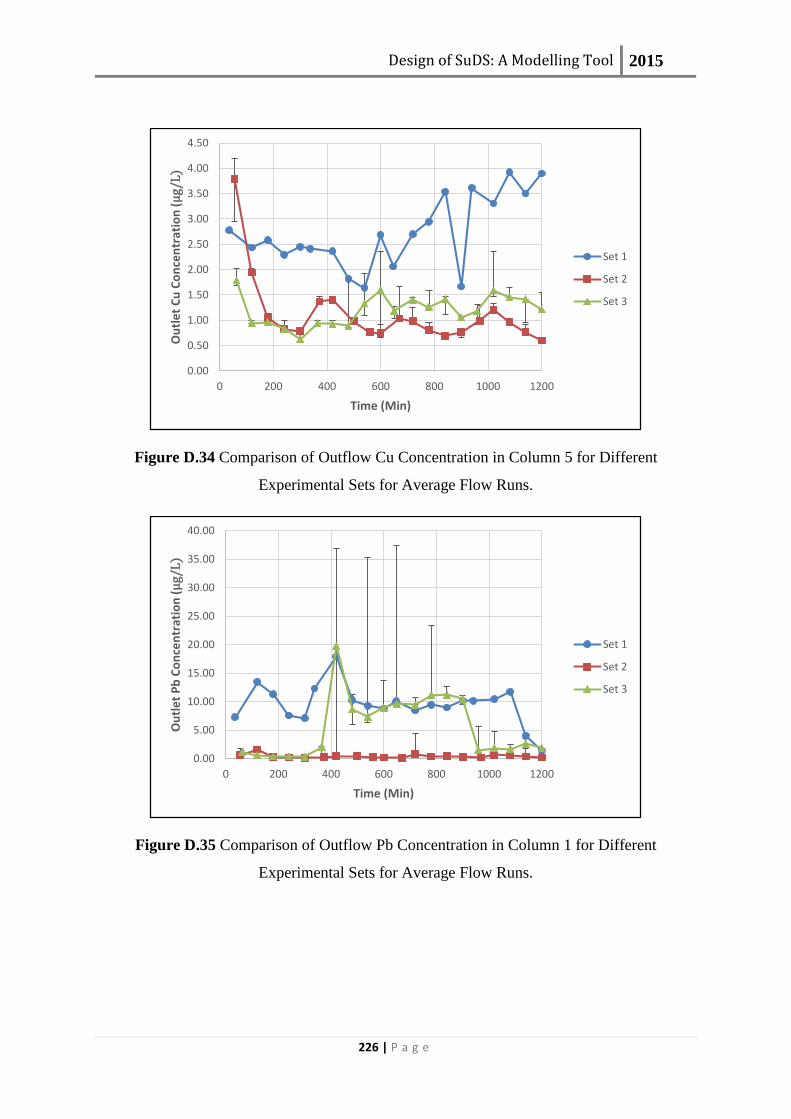
Design of SuDS: A Modelling Tool 2015
226 | P a g e
Figure D.34 Comparison of Outflow Cu Concentration in Column 5 for Different
Experimental Sets for Average Flow Runs.
Figure D.35 Comparison of Outflow Pb Concentration in Column 1 for Different
Experimental Sets for Average Flow Runs.
0.00
0.50
1.00
1.50
2.00
2.50
3.00
3.50
4.00
4.50
0 200 400 600 800 1000 1200
Ou
tle
t C
u C
on
cen
trat
ion
(μ
g/L
)
Time (Min)
Set 1
Set 2
Set 3
0.00
5.00
10.00
15.00
20.00
25.00
30.00
35.00
40.00
0 200 400 600 800 1000 1200
Ou
tle
t P
b C
on
cen
trat
ion
(μ
g/L
)
Time (Min)
Set 1
Set 2
Set 3

Design of SuDS: A Modelling Tool 2015
227 | P a g e
Figure D.36 Comparison of Outflow Pb Concentration in Column 2 for Different
Experimental Sets for Average Flow Runs.
Figure D.36 Comparison of Outflow Pb Concentration in Column 3 for Different
Experimental Sets for Average Flow Runs.
0.00
20.00
40.00
60.00
80.00
100.00
120.00
140.00
160.00
180.00
200.00
0 200 400 600 800 1000 1200
Ou
tle
t P
b C
on
cen
trat
ion
(μ
g/L
)
Time (Min)
Set 1
Set 2
Set 3
0.00
20.00
40.00
60.00
80.00
100.00
120.00
0 200 400 600 800 1000 1200
Ou
tle
t P
b C
on
cen
trat
ion
(μ
g/L
)
Time (Min)
Set 1
Set 2
Set 3

Design of SuDS: A Modelling Tool 2015
228 | P a g e
Figure D.37 Comparison of Outflow Pb Concentration in Column 4 for Different
Experimental Sets for Average Flow Runs.
Figure D.38 Comparison of Outflow Pb Concentration in Column 5 for Different
Experimental Sets for Average Flow Runs.
0.00
10.00
20.00
30.00
40.00
50.00
60.00
70.00
80.00
0 200 400 600 800 1000 1200
Ou
tle
t C
u C
on
cen
trat
ion
(μ
g/L
)
Time (Min)
Set 1
Set 2
Set 3
0.00
20.00
40.00
60.00
80.00
100.00
120.00
140.00
160.00
0 200 400 600 800 1000 1200
Ou
tle
t C
u C
on
cen
trat
ion
(μ
g/L
)
Time (Min)
Set 1
Set 2
Set 3

Design of SuDS: A Modelling Tool 2015
229 | P a g e
Figure D.39 Comparison of Outflow Zn Concentration in Column 1 for Different
Experimental Sets for Average Flow Runs.
Figure D.40 Comparison of Outflow Zn Concentration in Column 2 for Different
Experimental Sets for Average Flow Runs.
0.00
10.00
20.00
30.00
40.00
50.00
60.00
70.00
80.00
90.00
0 200 400 600 800 1000 1200
Ou
tle
t Zn
Co
nce
ntr
atio
n (μ
g/L
)
Time (Min)
Set 1
Set 2
Set 3
0.00
20.00
40.00
60.00
80.00
100.00
120.00
0 200 400 600 800 1000 1200
Ou
tle
t Zn
Co
nce
ntr
atio
n (μ
g/L
)
Time (Min)
Set 1
Set 2
Set 3

Design of SuDS: A Modelling Tool 2015
230 | P a g e
Figure D.41 Comparison of Outflow Zn Concentration in Column 3 for Different
Experimental Sets for Average Flow Runs.
Figure D.42 Comparison of Outflow Zn Concentration in Column 4 for Different
Experimental Sets for Average Flow Runs.
0.00
20.00
40.00
60.00
80.00
100.00
120.00
140.00
0 200 400 600 800 1000 1200
Ou
tle
t Zn
Co
nce
ntr
atio
n (μ
g/L
)
Time (Min)
Set 1
Set 2
Set 3
0.00
20.00
40.00
60.00
80.00
100.00
120.00
140.00
0 200 400 600 800 1000 1200
Ou
tle
t Z
n C
on
cen
trat
ion
(μ
g/L
)
Time (Min)
Set 1
Set 2
Set 3
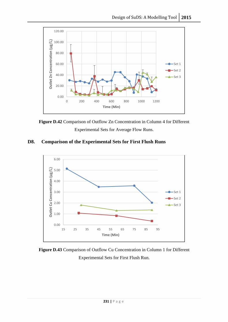
Design of SuDS: A Modelling Tool 2015
231 | P a g e
Figure D.42 Comparison of Outflow Zn Concentration in Column 4 for Different
Experimental Sets for Average Flow Runs.
D8. Comparison of the Experimental Sets for First Flush Runs
Figure D.43 Comparison of Outflow Cu Concentration in Column 1 for Different
Experimental Sets for First Flush Run.
0.00
20.00
40.00
60.00
80.00
100.00
120.00
0 200 400 600 800 1000 1200
Ou
tle
t Zn
Co
nce
ntr
atio
n (μ
g/L
)
Time (Min)
Set 1
Set 2
Set 3
0.00
1.00
2.00
3.00
4.00
5.00
6.00
15 25 35 45 55 65 75 85 95
Ou
tle
t C
u C
on
cen
trat
ion
(μ
g/L
)
Time (Min)
Set 1
Set 2
Set 3

Design of SuDS: A Modelling Tool 2015
232 | P a g e
Figure D.44 Comparison of Outflow Cu Concentration in Column 2 for Different
Experimental Sets for First Flush Run.
Figure D.45 Comparison of Outflow Cu Concentration in Column 3 for Different
Experimental Sets for First Flush Run.
0.00
1.00
2.00
3.00
4.00
5.00
6.00
7.00
8.00
15 25 35 45 55 65 75 85 95
Ou
tle
t C
u C
on
cen
trat
ion
(μ
g/L
)
Time (Min)
Set 1
Set 2
Set 3
0.00
2.00
4.00
6.00
8.00
10.00
12.00
15 25 35 45 55 65 75 85 95
Ou
tle
t C
u C
on
cen
trat
ion
(μ
g/L
)
Time (Min)
Set 1
Set 2
Set 3

Design of SuDS: A Modelling Tool 2015
233 | P a g e
Figure D.46 Comparison of Outflow Cu Concentration in Column 4 for Different
Experimental Sets for First Flush Run.
Figure D.47 Comparison of Outflow Cu Concentration in Column 5 for Different
Experimental Sets for First Flush Run.
0.00
0.50
1.00
1.50
2.00
2.50
3.00
3.50
4.00
4.50
5.00
15 25 35 45 55 65 75 85 95
Ou
tle
t C
u C
on
cen
trat
ion
(μ
g/L
)
Time (Min)
Set 1
Set 2
Set 3
0.00
1.00
2.00
3.00
4.00
5.00
6.00
7.00
8.00
9.00
15 25 35 45 55 65 75 85 95
Ou
tle
t C
u C
on
cen
trat
ion
(μ
g/L
)
Time (Min)
Set 1
Set 2
Set 3
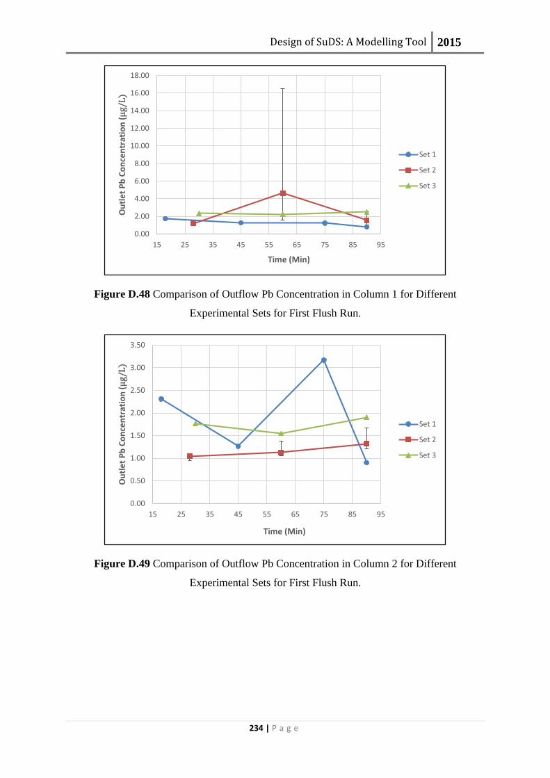
Design of SuDS: A Modelling Tool 2015
234 | P a g e
Figure D.48 Comparison of Outflow Pb Concentration in Column 1 for Different
Experimental Sets for First Flush Run.
Figure D.49 Comparison of Outflow Pb Concentration in Column 2 for Different
Experimental Sets for First Flush Run.
0.00
2.00
4.00
6.00
8.00
10.00
12.00
14.00
16.00
18.00
15 25 35 45 55 65 75 85 95
Ou
tle
t P
b C
on
cen
trat
ion
(μ
g/L
)
Time (Min)
Set 1
Set 2
Set 3
0.00
0.50
1.00
1.50
2.00
2.50
3.00
3.50
15 25 35 45 55 65 75 85 95
Ou
tle
t P
b C
on
cen
trat
ion
(μ
g/L
)
Time (Min)
Set 1
Set 2
Set 3

Design of SuDS: A Modelling Tool 2015
235 | P a g e
Figure D.50 Comparison of Outflow Pb Concentration in Column 3 for Different
Experimental Sets for First Flush Run.
Figure D.51 Comparison of Outflow Pb Concentration in Column 4 for Different
Experimental Sets for First Flush Run.
0.00
0.50
1.00
1.50
2.00
2.50
3.00
15 25 35 45 55 65 75 85 95
Ou
tle
t P
b C
on
cen
trat
ion
(μ
g/L
)
Time (Min)
Set 1
Set 2
Set 3
0.00
0.50
1.00
1.50
2.00
2.50
3.00
3.50
15 25 35 45 55 65 75 85 95
Ou
tle
t P
b C
on
cen
trat
ion
(μ
g/L
)
Time (Min)
Set 1
Set 2
Set 3

Design of SuDS: A Modelling Tool 2015
236 | P a g e
Figure D.52 Comparison of Outflow Pb Concentration in Column 5 for Different
Experimental Sets for First Flush Run.
Figure D.53 Comparison of Outflow Zn Concentration in Column 1 for Different
Experimental Sets for First Flush Run.
0.00
0.50
1.00
1.50
2.00
2.50
3.00
3.50
15 25 35 45 55 65 75 85 95
Ou
tle
t P
b C
on
cen
trat
ion
(μ
g/L
)
Time (Min)
Set 1
Set 2
Set 3
0.00
10.00
20.00
30.00
40.00
50.00
60.00
15 25 35 45 55 65 75 85 95
Ou
tle
t Zn
Co
nce
ntr
atio
n (μ
g/L
)
Time (Min)
Set 1
Set 2
Set 3

Design of SuDS: A Modelling Tool 2015
237 | P a g e
Figure D.54 Comparison of Outflow Zn Concentration in Column 2 for Different
Experimental Sets for First Flush Run.
Figure D.55 Comparison of Outflow Zn Concentration in Column 3 for Different
Experimental Sets for First Flush Run.
0.00
10.00
20.00
30.00
40.00
50.00
60.00
70.00
80.00
90.00
15 25 35 45 55 65 75 85 95
Ou
tle
t Zn
Co
nce
ntr
atio
n (μ
g/L
)
Time (Min)
Set 1
Set 2
Set 3
0.00
20.00
40.00
60.00
80.00
100.00
120.00
140.00
15 25 35 45 55 65 75 85 95
Ou
tle
t Zn
Co
nce
ntr
atio
n (μ
g/L
)
Time (Min)
Set 1
Set 2
Set 3

Design of SuDS: A Modelling Tool 2015
238 | P a g e
Figure D.56 Comparison of Outflow Zn Concentration in Column 4 for Different
Experimental Sets for First Flush Run.
Figure D.56 Comparison of Outflow Zn Concentration in Column 5 for Different
Experimental Sets for First Flush Run.
0.00
10.00
20.00
30.00
40.00
50.00
60.00
70.00
80.00
15 25 35 45 55 65 75 85 95
Ou
tle
t Zn
Co
nce
ntr
atio
n (μ
g/L
)
Time (Min)
Set 1
Set 2
Set 3
0.00
10.00
20.00
30.00
40.00
50.00
60.00
70.00
80.00
15 25 35 45 55 65 75 85 95
Ou
tle
t Zn
Co
nce
ntr
atio
n (μ
g/L
)
Time (Min)
Set 1
Set 2
Set 3

Design of SuDS: A Modelling Tool 2015
239 | P a g e
D9. Van Genuchten Parameters
Column 1 (Soil/Sand 10cm)
Table D.4 Van Genuchten Parameters for Column 1 (Soil/Sand 15 cm)
Van Genuchtens Parameters
θsat (m3/m3) 0.452
θres (m3/m3) 0.05185
Alpha 0.044
n 3.3166
m 0.698486
Column 1 (Soil/Sand 45cm)
Table D.5 Van Genuchten Parameters for Column 1 (Soil/Sand 55 cm)
Van Genuchtens Parameters
θsat (m3/m3) 0.4799
θres (m3/m3) 0.048581
Alpha 0.050602
n 3.0298
m 0.669945
Column 2 (Soil/Sand 10cm)
Table D.6 Van Genuchten Parameters for Column 2 (Soil/Sand 15 cm)
Van Genuchtens Parameters
θsat (m3/m3) 0.506
θres (m3/m3) 0.051815
Alpha 0.063814
n 2.6204
m 0.618379
Column 2 (Soil/Sand 45cm)
Table D.7 Van Genuchten Parameters for Column 2 (Soil/Sand 55 cm)
Van Genuchtens Parameters
θsat (m3/m3) 0.47699
θres (m3/m3) 0.047652
Alpha 0.052005
n 2.9639
m 0.662607

Design of SuDS: A Modelling Tool 2015
240 | P a g e
Column 2 (Sand 75cm)
Table D.8 Van Genuchten Parameters for Column 2 (Sand 75cm)
Van Genuchtens Parameters
θsat (m3/m3) 0.3055
θres (m3/m3) 0.011
Alpha 0.07
n 6.7
m 0.8507
Column 5 (Soil/Sand 10cm)
Table D.9 Van Genuchten Parameters for Column 5 (Soil/Sand 15 cm)
Van Genuchtens Parameters
θsat (m3/m3) 0.482
θres (m3/m3) 0.047819
Alpha 0.055673
n 2.8943
m 0.654493
Column 5 (Soil/Sand 45cm)
Table D.10 Van Genuchten Parameters for Column 5 (Soil/Sand 55 cm)
Van Genuchtens Parameters
θsat (m3/m3) 0.452
θres (m3/m3) 0.051815
Alpha 0.044
n 3.3166
m 0.698486
Column 5 (Sand 75cm)
Table D.11 Van Genuchten Parameters for Column 5 (Sand 75 cm)
Van Genuchtens Parameters
θsat (m3/m3) 0.34312
θres (m3/m3) 0.019755
Alpha 0.074234
n 6.691
m 0.85

Design of SuDS: A Modelling Tool 2015
241 | P a g e
E. PUBLICATIONS AND
CONFERENCES Quinn, R. and Dussaillant A. Predicting pollutant retention in SUDS, with a rain garden
application. 2012. BHS National Symposium. 3-6 July. DOI: 0.7558/bhs.2012.ns45
Quinn, R. and Dussaillant A. Predicting heavy metal retention in Sustainable Urban Drainage
Systems. 2012. SUDSnet International Conference. 4-5 September.
Quinn, R. and Dussaillant A. 2014. Heavy metal retention and bypass in Sustainable Drainage
Systems: application to bioretention facilities. Clean. 42(2), pp.160-168.
Quinn, R. and Dussaillant, A. 2014. Predicting infiltration pollutant retention in bioretention
sustainable drainage systems: model development and validation. Hydrology Research, 45 (6),
pp. 855-867.