EVALUATION OF EFFECTIVE WIDTH AND DISTRIBUTION FACTORS FOR GFRP BRIDGE DECKS SUPPORTED ON STEEL GIRDERS

by

Jonathan Moses

B.S.C.E., University of Pittsburgh, 2004

Submitted to the Graduate Faculty of

The School of Engineering in partial fulfillment

of the requirements for the degree of

Master of Science in Civil Engineering

University of Pittsburgh

2005

UNIVERSITY OF PITTSBURGH

SCHOOL OF ENGINEERING

This thesis was presented

by

Jonathan Moses

It was defended on

September 16, 2005

and approved by

Thesis Advisor: Dr. Kent A. Harries, Assistant Professor, Dept. of Civil & Environmental Engineering

Committee Member: Dr. Christopher Earls, Chairman, Associate Professor & William Kepler Whiteford Faculty Fellow,

Dept. of Civil & Environmental Engineering

Committee Member: Dr. Amir Koubaa, Academic Coordinator, Department of Civil & Environmental Engineering

ii

ABSTRACT

EVALUATION OF EFFECTIVE WIDTH AND DISTRIBUTION FACTORS FOR GFRP BRIDGE DECKS SUPPORTED ON STEEL GIRDERS

Jonathan Moses, M.S.

University of Pittsburgh, 2005

Glass fiber reinforced polymer (GFRP) bridge deck systems offer an attractive alternative

to concrete decks, particularly for bridge rehabilitation projects. Current design practice treats

GFRP deck systems in a manner similar to concrete decks. The results of this study, however,

indicate that this may result in non-conservative design values for the bridge girders. Results

from a number of in situ load tests of three steel girder bridges having the same (GFRP) deck

system are used to determine the degree of composite action that may be developed and the

transverse distribution of wheel loads that may be assumed for such structures. Results indicate

that appropriately conservative design values may be found by assuming no composite action

between GFRP deck and steel girder and using the lever rule to determine transverse load

distribution. When used to replace an existing concrete deck, the lighter GFRP deck will result in

lower total loads applied to the bridge structure, although, due to the decreased effective width

and increased distribution factors, local flange stresses and particularly the live load-induced

stress range is likely to be increased. Thus, existing fatigue-prone details may become a concern

and require attention in design.

iii

TABLE OF CONTENTS 1.0 INTODUCTION AND LITERATURE REVIEW ............................................................. 1

1.1 REINFORCED CONCRETE BRIDGE DECKS ........................................................... 3

1.2 FIBER REINFORCED POLYMER BRIDGE DECKS................................................. 3

1.2.1 Existing GFRP Bridge Decks in Use ...................................................................... 5

1.3 DESIGN PARAMETERS FOR GFRP DECKS........................................................... 11

1.3.1 Effective Width of Deck ....................................................................................... 11

1.3.1.1 Calculating Effective Width from In-situ Tests................................................ 12

1.3.2 Engaging Effective Deck Width with Shear Connectors...................................... 14

1.3.2.1 Push-off Tests to Determine Stud Capacity...................................................... 15

1.3.2.2 Engaging Effective Deck Width with Adhesively Bonded Deck Systems....... 19

1.3.3 Moment Distribution Factors................................................................................ 20

1.3.3.1 Calculating Moment Distribution Factors from In-situ Tests........................... 22

1.4 SCOPE OF THESIS ..................................................................................................... 23

2.0 DESCRIPTIONS OF BRIDGES REPORTED IN THIS STUDY................................... 24

2.1 TYPICAL GFRP DECK PANEL INSTALLATION................................................... 26

2.2 FAIRGROUND ROAD BRIDGE ................................................................................ 29

2.3 BOYER BRIDGE ......................................................................................................... 31

2.4 SOUTH CAROLINA S655 BRIDGE .......................................................................... 33

3.0 OBSERVED RESULTS OF LOAD TESTS .................................................................... 35

iv

3.1 APPARENT EFFECTIVE WIDTH ............................................................................. 35

3.2 MOMENT DISTRIBUTION FACTORS FROM IN-SITU TESTS ............................ 38

3.3 IMPLICATIONS FOR NEW CONSTRUCTION USING GFRP DECKS ................. 41

3.3.1 Composite Behavior.............................................................................................. 41

3.3.2 Moment Distribution Factors................................................................................ 42

3.4 IMPLICATIONS FOR REPLACING CONCRETE DECKS WITH GFRP DECKS . 42

4.0 ILLUSTRATIVE EXAMPLE – SUPERSTRUCTURE STRESSES............................... 44

4.1 PROTOTYPE BRIDGE SECTIONAL PROPERTIES................................................ 44

4.1.1 Plastic Moment Calculation for Composite GFRP Case ...................................... 49

4.2 APPLIED LOADING AND LOAD CASES................................................................ 53

4.3 STRESSES IN STEEL GIRDERS ............................................................................... 55

4.4 RETROFIT SCENARIOS ............................................................................................ 58

4.5 AASHTO FATIGUE CRITERIA................................................................................. 60

5.0 CONCLUSIONS AND RECOMMENDATIONS ........................................................... 64

5.1 RECOMMENDATIONS.............................................................................................. 65

APPENDIX A............................................................................................................................... 67

APPENDIX B-1............................................................................................................................ 70

APPENDIX B-2............................................................................................................................ 74

BIBLIOGRAPHY......................................................................................................................... 79

v

LIST OF TABLES Table 1-1: Existing Bridges with GFRP Decks .............................................................................. 6

Table 1-2: Effective Width Calculations ...................................................................................... 13

Table 1-3: Shear Stud Capacities for Various Tests ..................................................................... 18

Table 2-1: Summary of Bridge Details......................................................................................... 26

Table 3-1: Comparison of AASHTO and Observed Effective Width Values .............................. 36

Table 3-2: Comparison of AASHTO and Observed Moment Distribution Factor Values........... 39

Table 4-1: Material and Member Properties................................................................................. 46

Table 4-2: Plastic Moment Capacity Calculation ......................................................................... 52

Table 4-3: Design Loading and Moments (see Appendix B-2 for details)................................... 54

Table 4-4: Calculated Stress Ranges - STRENGTH I .................................................................. 56

Table 4-5: Calculated Stress Ranges - SERVICE I ...................................................................... 56

Table 4-6: Calculated Stress Ranges – FATIGUE ....................................................................... 56

Table 4-7: Ratios of Post-Retrofit Stresses to Pre-Retrofit Stresses............................................. 59

Table 4-8: AASHTO Fatigue Thresholds ..................................................................................... 62

vi

LIST OF FIGURES Figure 1-1: Schematic of DuraSpan Deck Panel (MMC).............................................................. 5

Figure 1-2: Cross-Section of GFRP Composite Section.............................................................. 13

Figure 1-3: Push-off Test Specimen ............................................................................................ 17

Figure 1-4: Push-off Test Specimen in Load Frame (Yulismana 2005)...................................... 17

Figure 2-1: Transverse Section GFRP Deck Geometry and Dimensions.................................... 25

Figure 2-2: Installation of GFRP deck panels (Boyer Bridge) .................................................... 28

Figure 2-3: Fairground Road Bridge............................................................................................ 30

Figure 2-4: Boyer Bridge .............................................................................................................. 32

Figure 2-5: South Carolina SC655 Bridge.................................................................................... 34

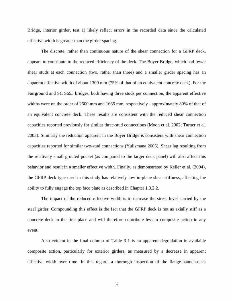
Figure 4-1: Cross-section of Composite Beam (Case 1) .............................................................. 48

Figure 4-2: Cross-section of Composite Beam (Case 3) .............................................................. 48

Figure 4-3: Loading Condition of Top Face Plate ........................................................................ 50

Figure 4-4: Determination of Plastic Section................................................................................ 51

vii

ACKNOWLEDGEMENTS

I would like to thank Dr. Earls for believing in me and giving me the opportunity to do

the research and the subsequent thesis. I would like to thank Dr. Harries for the many hours of

review, comments, and guidance provided me throughout and for giving me the necessary push

to see this thesis to conclusion. I would also like to thank Dr. Koubaa for being on my committee

and assisting me with the process. Finally, I would like to thank Joe Yulismana for teaching me

everything I know about composites and testing in the lab.

viii

1.0 INTODUCTION AND LITERATURE REVIEW

The deteriorating state of the Nation’s bridge infrastructure is well documented. Fewer

resources are available to maintain and repair a growing list of deteriorated structures.

Deterioration of bridge structures may result from age, exposure to adverse environments

(particularly the use of de-icing salts), increasing traffic volumes and loading, or specific

extreme events such as truck impacts. To address the issue of deteriorating structures, new cost

effective technology which can extend the service life of such structures is necessary. In recent

years, high-performance fiber reinforced polymer (FRP) composite materials have been

identified as excellent candidates for rehabilitating aging bridge structures.

According to data from the National Bridge Inventory (NBI 2003), of the nation’s

approximately 615,000 bridges, over 26% were either not structurally sufficient or functionally

obsolete. These numbers were significantly worse for Pennsylvania, with an estimated 42% of

the state’s approximately 22,000 bridges being deemed either not structurally sufficient or

functionally obsolete. A major cause of the structural deficiency of existing bridges is excessive

deterioration of conventional concrete decks. Deterioration is often worse in northern states

where large amounts of de-icing salt are applied to the deck surfaces of bridges during the winter

months. It has been estimated (FHWA 2004) that more than 88,000,000 m2 (approximately 1

billion square feet) of bridge deck is currently in need of replacement at an estimated cost of over

$30 billion. Additionally, 19% of the nation’s bridges are either posted for load or in need of

posting (NBI 2003).

1

There are a variety of different deck types to choose from at present. Traditionally,

reinforced concrete decks are used in most bridge structures. Another type of deck that has been

in use for more than 60 years is the concrete filled steel grid deck. More recent innovations

aimed at reducing deck weight include orthotropic steel deck systems and GFRP bridge deck

panels, which are both becoming more commonly used for bridge deck replacement.

The use of GFRP bridge deck elements has been introduced and demonstrated as a viable

means of both deck replacement and new deck construction. Since 1998, 83 bridges in the

United States have been constructed or had their existing decks replaced with GFRP decks

(Hooks and O’Connor 2004). GFRP decks are attractive because of their minimal installation

time, high strength-to-weight ratios, and excellent tolerance to frost and de-icing salts. Their light

weight, and thus reduced dead load, is particularly attractive for rehabilitating posted structures

since the replacement of heavy conventional concrete decking with lighter weight GFRP decking

may translate to additional live load carrying capacity for the bridge system.

Curiously, despite this latter advantage, most of the bridges currently employing GFRP

decks in their designs are new construction as opposed to rehabilitation applications. Using

GFRP deck panels in a new design may not be as practical as using them for rehabilitation

projects. The deck panels themselves are initially more expensive than their equivalent concrete

slab counterparts and there is not likely to be a great savings to be had from the reduced dead

load. The installation time, however, can be as little as one working day for a relatively short

span bridge. This is a significant time savings over placing a concrete deck and may warrant the

selection of a GFRP deck for new construction in some circumstances.

For rehabilitation, however, the reduced dead load of a GFRP deck may represent a

significant advantage possibly allowing load posting to be removed or an increase in the bridge

2

rating to be made. For example, the deck system reported in this work weighs approximately one

fifth of what a comparable concrete deck would weigh. Similarly, for historic bridge structures,

the reduced deck load may permit increased load rating without altering the original state of the

bridge. The rapid installation of a GFRP deck also reduces bridge closure time for a

rehabilitation project.

1.1 REINFORCED CONCRETE BRIDGE DECKS

Conventional concrete bridge deck design is largely prescriptive; guided by general

proportions as promulgated by the AASHTO (1996 and 2004) specifications. Deck thickness and

reinforcing details are selected based on longitudinal girder spacing. Strength and serviceability

of bridge systems having concrete decks have been established by heuristic and theoretical

means and the adequacy of such approaches have been borne out by engineering experience as

well as experimentally. The spatial nature of concrete deck systems allows the deck to transmit

loads laterally to the primary longitudinal girders while composite action between the deck and

the underlying girders may also be developed to permit the deck to assist in resisting the

longitudinal flexure in the span. These characteristics of a bridge deck are quantified in a design

context through the definition of the moment distribution factor and the effective width,

respectively. These characteristics will be discussed further below in relation to both new

construction and rehabilitation.

1.2 FIBER REINFORCED POLYMER BRIDGE DECKS

Glass fiber reinforced polymer (GFRP) composite bridge deck systems are beginning to

gain acceptance as light weight and durable alternatives to concrete decks (Black 2003).

3

Although many existing demonstration projects are based on new bridges, (Hooks and O’Connor

2004), GFRP decks hold their greatest promise as a method of deck replacement for older

structures. GFRP bridge decks capable of replacing 200 to 250 mm (8 to 10 in.) thick reinforced

concrete decks (weighing 4.8 to 6.0 kPa (100 to 125 psf)) typically weigh about 0.96 kPa (20

psf) without a wearing surface, representing a significant savings in the dead load of the

superstructure.

Although there are a variety of proprietary GFRP bridge deck systems that have been

proposed and demonstrated, this work focuses on those systems designed to span transversely

between longitudinal bridge girders and carry traffic loads in a manner similar to a “one way”

concrete deck. Such GFRP deck systems have taken two fundamental forms (Turner 2003):

1. A series of closed-shape pultruded GFRP tubes that are sandwiched between top and

bottom face plates. The tubes and face plate components are assembled using a structural

adhesive. (examples include Crocker et al. 2002 and Zhou et al. 2002). A variation on

this form using an arrangement of perpendicular tubes and no face plates is presented by

Chandrashekhara and Nanni (2000).

2. A series of interlocking pultruded shapes which include both face plates and web

elements (examples include Motley et al. 2002 and GangaRao et al. 1999). Such systems

are generally more versatile and have better final product quality control than adhesively

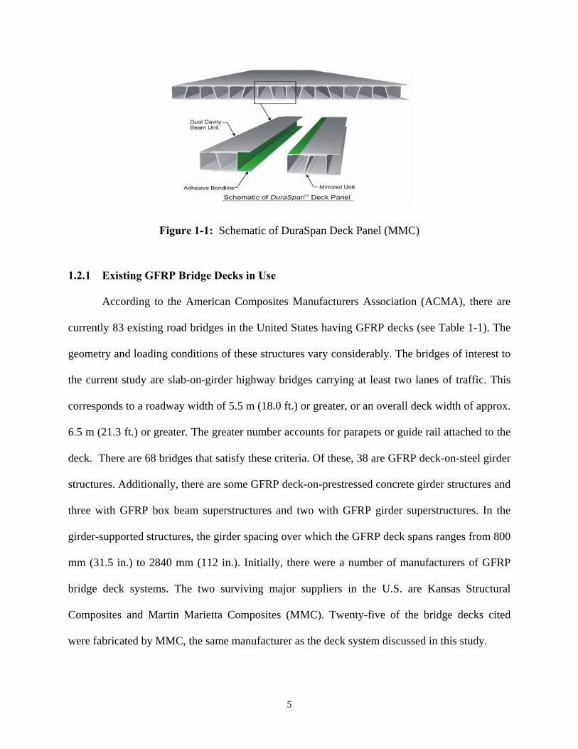
assembled tubes. An example of this type of deck is the Martin Marietta Composites

DuraSpan Deck Panel considered in this work (see Figure 1-1).

4

5

1.2.1 Existing GFRP Bridge Decks in Use

According to the American Composites Manufacturers Association (ACMA), there are

currently 83 existing road bridges in the United States having GFRP decks (see Table 1-1). The

geometry and loading conditions of these structures vary considerably. The bridges of interest to

the current study are slab-on-girder highway bridges carrying at least two lanes of traffic. This

corresponds to a roadway width of 5.5 m (18.0 ft.) or greater, or an overall deck width of approx.

6.5 m (21.3 ft.) or greater. The greater number accounts for parapets or guide rail attached to the

deck. There are 68 bridges that satisfy these criteria. Of these, 38 are GFRP deck-on-steel girder

structures. Additionally, there are some GFRP deck-on-prestressed concrete girder structures and

three with GFRP box beam superstructures and two with GFRP girder superstructures. In the

girder-supported structures, the girder spacing over which the GFRP deck spans ranges from 800

mm (31.5 in.) to 2840 mm (112 in.). Initially, there were a number of manufacturers of GFRP

bridge deck systems. The two surviving major suppliers in the U.S. are Kansas Structural

Composites and Martin Marietta Composites (MMC). Twenty-five of the bridge decks cited

were fabricated by MMC, the same manufacturer as the deck system discussed in this study.

Figure 1-1: Schematic of DuraSpan Deck Panel (MMC)

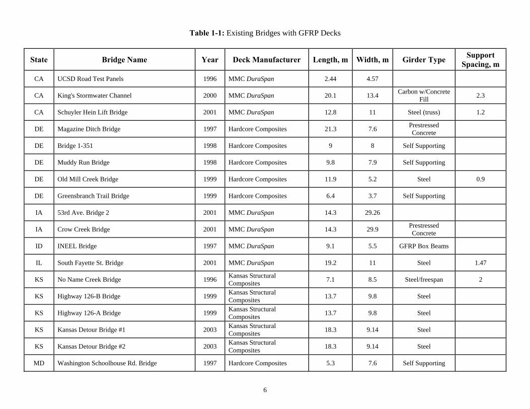
Table 1-1: Existing Bridges with GFRP Decks

State Bridge Name Year Deck Manufacturer Length, m Width, m Girder Type Support Spacing, m

CA UCSD Road Test Panels 1996 MMC DuraSpan 2.44 4.57

CA King's Stormwater Channel 2000 MMC DuraSpan 20.1 13.4 Carbon w/Concrete Fill 2.3

CA Schuyler Hein Lift Bridge 2001 MMC DuraSpan 12.8 11 Steel (truss) 1.2

DE Magazine Ditch Bridge 1997 Hardcore Composites 21.3 7.6 Prestressed Concrete

DE Bridge 1-351 1998 Hardcore Composites 9 8 Self Supporting

DE Muddy Run Bridge 1998 Hardcore Composites 9.8 7.9 Self Supporting

DE Old Mill Creek Bridge 1999 Hardcore Composites 11.9 5.2 Steel 0.9

DE Greensbranch Trail Bridge 1999 Hardcore Composites 6.4 3.7 Self Supporting

IA 53rd Ave. Bridge 2 2001 MMC DuraSpan 14.3 29.26

IA Crow Creek Bridge 2001 MMC DuraSpan 14.3 29.9 Prestressed Concrete

ID INEEL Bridge 1997 MMC DuraSpan 9.1 5.5 GFRP Box Beams

IL South Fayette St. Bridge 2001 MMC DuraSpan 19.2 11 Steel 1.47

KS No Name Creek Bridge 1996 Kansas Structural Composites 7.1 8.5 Steel/freespan 2

KS Highway 126-B Bridge 1999 Kansas Structural Composites 13.7 9.8 Steel

KS Highway 126-A Bridge 1999 Kansas Structural Composites 13.7 9.8 Steel

KS Kansas Detour Bridge #1 2003 Kansas Structural Composites 18.3 9.14 Steel

KS Kansas Detour Bridge #2 2003 Kansas Structural Composites 18.3 9.14 Steel

MD Washington Schoolhouse Rd. Bridge 1997 Hardcore Composites 5.3 7.6 Self Supporting

6

Table 1-1 (continued)

State Bridge Name Year Deck Manufacturer Length, m Width, m Girder Type Support Spacing, m

MD Wheatley Rd. Bridge 2000 Hardcore Composites 10.36 7.3 Self Supporting

MD MD 24 Over Deer Creek Bridge 2001 MMC DuraSpan 39 9.8 Steel 1.2

MD Snouffer School Rd. Bridge 2001 Hardcore Composites 8.84 10.06 Self Supporting

ME Milbridge Municipal Pier Bridge 2000 Univ. of Maine 53.34 4.88

ME Skidmore Bridge 2000 Kenway Corp. 18.9 7.01 Steel

MI Bridge St. Over Rouge River 2001 Mitsubishi Chemical 60.35 9.14

MO St. John's Street Bridge 2000 Kansas Structural Composites 8.23 7.92 Steel

MO Jay Street Bridge 2000 Kansas Structural Composites 8.23 7.92 Steel

MO St. Francis Street Bridge 2000 Kansas Structural Composites 7.92 8.53 Freespan

NC Service Route 1627 Bridge Over Mill Creek 2001 MMC DuraSpan 12.2 7.62 Steel 1.19

NY Route 248 Bridge Over Bennetts Creek 1998 Hardcore Composites 7.62 10.1 Self Supporting 7.62

NY Route 367 Bridge Over Bentley Creek 1999 Hardcore Composites 42.7 7.6 Steel Floor Beam 4.3

NY Cayuta Creek Bridge 2000 Hardcore Composites 39.3 8.8 Steel 1.8

NY South Broad St. Bridge 2000 Hardcore Composites 36.6 8.8 Steel

NY SR 418 Over Schroon River Bridge 2000 MMC DuraSpan 48.8 7.9 Steel - Floorbeams & Stringers 1.2

NY Osceola Rd. (Rt. 46) Over East Branch Salmon River Bridge 2001 MMC DuraSpan 10 7.9 Steel 1.25

NY Triphammer Rd. Bridge Over Conesus Lake Outlet 2001 Hardcore Composites 12.2 10.1 GFRP Box Beams

NY Route 36 Over Tributary to Troups Creek 2001 Kansas Structural Composites 9.75 11.28

7

Table 1-1 (continued)

State Bridge Name Year Deck Manufacturer Length, m Width, m Girder Type Support Spacing, m

NY County Rd. 153 2002 Hardcore Composites 16.5 8.2

OH Smith Creek Bridge (TECH-21) 1997 MMC DuraSpan 10.1 7.3 GFRP Box Beams 2.4

OH Shawnee Creek Bridge 1997 Creative Pultrusions Superdeck 7.3 3.66 Railway Bridge

Beams

OH Woodington Run Bridge 1999 MMC DuraSpan 15.2 14 Galvanized Steel 2.5

OH Salem Bridge (1) 1999 Creative Pultrusions Superdeck 51.2 15.24 Steel 2.7

OH Salem Bridge (2) 1999 Hardcore Composites 51.2 15.24 Steel 2.7

OH Salem Bridge (3) 1999 Infrastructure Composites Int'l 17.68 15.24 Steel 2.7

OH Sintz Rd. Bridge 2000 Hardcore Composites 18.9 9.14 Steel

OH Westbrook Road Bridge Over Dry Run Creek 2000 Hardcore Composites 10.36 10.1 Self Supporting

OH Highway 14 Over Elliot Run 2000 Hardcore Composites 11.9 7.9 Steel

OH Five Mile Road Bridge #0171 2000 Hardcore Composites 13.4 8.5 AASHTO Type II 2.2

OH Five Mile Road Bridge #0087 2001 Hardcore Composites 14.3 9.14 AASHTO Type II 2.2

OH Five Mile Road Bridge #0071 2001 Hardcore Composites 13.1 9.14 AASHTO Type II 2.2

OH Shaffer Road Bridge 2001 Hardcore Composites 53.3 5.2 Steel

OH Stelzer Road Bridge 2001 Fiber Reinforced Systems Inc. 118 10.7 2.1

OH Spaulding Road Bridge 2001 Hardcore Composites 25.3 17.1 Concrete

OH Tyler Road Bridge Over Bokes Creek 2001 Fiber Reinforced Systems Inc. 36.6 6.1 Steel

OH Fairground Road Bridge 2002 MMC DuraSpan 67.4 9.75 Steel 2.84

8

Table 1-1 (continued)

State Bridge Name Year Deck Manufacturer Length, m Width, m Girder Type Support Spacing, m

OH Cats Creek Bridge 2002 MMC DuraSpan 24.7 7.3

OH Hotchkiss Road Bridge 2003 MMC DuraSpan 19.8 8.53

OH Hudson Road/Wolf Creek Bridge 2003 MMC DuraSpan 35.7 10.36

OH Hales Branch Road Bridge 2003 MMC DuraSpan 19.8 7.3

OH County Line Road Bridge Over Tiffin River 2003 MMC DuraSpan 57 8.53

OR Lewis and Clarke Bridge 2001 MMC DuraSpan 37.8 6.4 Steel (truss) 0.8

OR Old Young's Bay Bridge 2002 MMC DuraSpan 53.6 6.4 Steel (truss) 1.5

OR US 101 Over Siuslaw River 2003 N/A 46.9 8.53

PA Rowser Farm Bridge 1998 Creative Pultrusions Superdeck 4.88 3.66 GFRP I-Beam

PA Wilson's Bridge 1998 Hardcore Composites 19.8 4.9 Steel Floor Beam

PA SR 4003 - Laurel Run Rd. Bridge 1998 Creative Pultrusions Superdeck 6.7 7.9 Steel 0.89

PA SR 4012 - Boyer's Bridge Over Slippery Rock Creek 2001 MMC DuraSpan 13 7.9 Steel 1.8

PA SR 1037 - Dubois Creek Bridge 2001 Hardcore Composites 6.7 10.1 Self Supporting

PA TR 565 - Dunning Creek Bridge 2002 MMC DuraSpan 27.7 6.7 Steel

SC SC655 - Greenwood Road Bridge Over Norfolk Southern Railway 2001 MMC DuraSpan 18.3 11.4 Steel 2.4

VA Troutville Weigh Station Ramp I-82 1999 Creative Pultrusions Superdeck 6.1 6.1

WA Chief Joseph Dam Bridge 2003 N/A 90.8 9.75

WI US 151 Over Highway 26 Bridge 2003 Hughes Bros., Inc. 32.6 13.1

9

Table 1-1 (continued)

State Bridge Name Year Deck Manufacturer Length, m Width, m Girder Type Support Spacing, m

WI US 151 Over Highway 26 Bridge 2003 Diversified Composites 65.2 11.9

WV Wickwire Run Bridge 1997 Creative Pultrusions Superdeck 9.1 6.7 Steel 1.8

WV Laurel Lick Bridge 1997 Creative Pultrusions Superdeck 6.1 4.88 GFRP I-Beam

WV Market Street Bridge 2000 Creative Pultrusions Superdeck 54.9 17.1 Steel 2.6

WV Hanover Bridge 2001 Kansas Structural Composites 36.6 8.5 Steel 1.3

WV Boy Scout Camp Bridge 2001 Hardcore Composites 9.4 7.9 Steel 1.1

WV Montrose Bridge 2001 Hardcore Composites 11.9 8.5 Steel 1.4

WV West Buckeye Bridge 2001 Kansas Structural Composites 45.1 11 Steel

WV Katty Truss Bridge 2002 Creative Pultrusions Superdeck 27.4 4.3 Steel 1.8

WV La Chein Bridge 2003 Bedford Reinforced Plastics 9.75 7.3 Steel 1.3

WV Howell's Mill Bridge 2003 MMC DuraSpan 74.7 10.1 Steel 2.1

WV Goat Farm Bridge 2003 Kansas Structural Composites 12.2 4.6 Steel 1.2

The information contained in this table was collected from a variety of sources. Most data however, may be found in the following references: http://www.mdacomposites.org/mda/Bridge_Report_VEH.htm, West Virginia University (2001), Martin Marietta Composites (2001), Hodgson et al. (2002) and FHWA (2002).

10

1.3 DESIGN PARAMETERS FOR GFRP DECKS

There are several important differences in behavior between conventional reinforced

concrete bridge decks and GFRP bridge decks. GFRP bridge decks do not act in a fully

composite manner with the underlying girders, as it is assumed concrete decks may. Thus, the

effective width is an important parameter to consider in deck replacements with GFRP deck

panels. Another important parameter to consider is the moment distribution factor for the bridge.

The moment distribution factor (DF) is a measure of the proportion of the live load that each

girder must be designed to resist. There is a different distribution factor for interior and exterior

girders.

1.3.1 Effective Width of Deck

In a composite deck-girder system, the effective width of the deck is the portion of the

deck assumed to be contributing to the flexural capacity of the longitudinal girder through the

development of a uniform longitudinal stress field. Such an approach is adopted as a

simplification allowing for the neglect of the actual “shear lag” in the deck plate during flexure.

The deck is engaged by providing interfacial continuity between the deck and girders through the

use of shear connectors. The width of deck that may be engaged in flexure must be evaluated in

order to optimize the design of the longitudinal girder system. In new construction using GFRP

decks, many demonstration projects have not relied on composite action between the deck and

girders. Since these are largely demonstration projects, the girders have been designed to permit

the eventual replacement of the demonstration GFRP deck with a heavier conventional concrete

deck, often assuming that no composite behavior will be available (Turner et al. 2004).

Nonetheless, shear connectors have been provided in all existing applications and a measure of

composite action under service loads is therefore achieved (Keelor et al. 2004).

11

For interior steel girders having a composite concrete deck, the effective concrete flange

width contributing to the flexural capacity of the girder is prescribed (AASHTO (2004) Clause

4.6.2.6.1) to be the lesser of:

1. one quarter of the effective span length;

2. 12 times the depth of the concrete deck plus one half the width of the top flange of the

girder; or,

3. the average spacing of adjacent beams (denoted S).

Differences between the effective width that may be engaged between concrete and

replacement GFRP decks may be a critical consideration in deck replacement. If an existing

bridge behaves in a composite manner, the replacement deck must also permit this behavior;

otherwise girder stresses due to live loads will increase significantly. While it is true that dead

load stresses may be significantly reduced in the case of a GFRP deck, this does not affect the

live load induced stress range which may also affect fatigue-sensitive details.

1.3.1.1 Calculating Effective Width from In-situ Tests

The calculations for effective width in this study are based on fundamental mechanics and the

assumption that plane sections remain plane. The calculations assumed fully composite action

between the steel stringers and the GFRP deck, although it is apparent from the data that the

GFRP deck is not acting in a fully composite manner.

The effective width of deck is calculated from a plane sections analysis of the composite

girder calculating the location of the neutral axis based on in situ girder strains and applying

girder and deck material properties. For a composite section, the neutral axis is located using

12

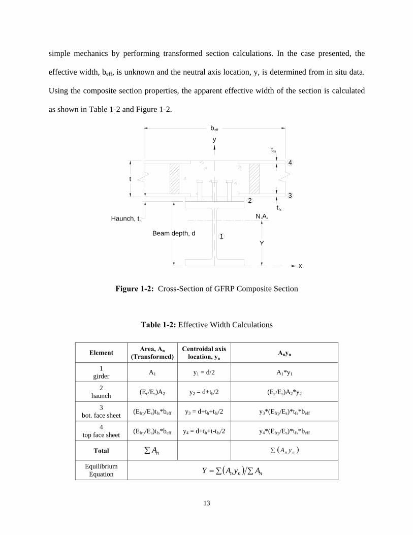
simple mechanics by performing transformed section calculations. In the case presented, the

effective width, beff, is unknown and the neutral axis location, y, is determined from in situ data.

Using the composite section properties, the apparent effective width of the section is calculated

as shown in Table 1-2 and Figure 1-2.

Haunch, t

t

t

Beam depth, d

h

1Y

x

N.A.fs

beff

yt

4

32

fs

Figure 1-2: Cross-Section of GFRP Composite Section

Table 1-2: Effective Width Calculations

Element Area, An (Transformed)

Centroidal axis location, yn

Anyn

1 girder A1 y1 = d/2 A1*y1

2 haunch (Ec/Es)A2 y2 = d+th/2 (Ec/Es)A2*y2

3 bot. face sheet (Efrp/Es)tfs*beff y3 = d+th+tfs/2 y3*(Efrp/Es)*tfs*beff

4 top face sheet (Efrp/Es)tfs*beff y4 = d+th+t-tfs/2 y4*(Efrp/Es)*tfs*beff

Total ∑ nA ( )∑ nn yA

Equilibrium Equation ( ) ∑∑= nnn AyAY

13

For each of the bridges in this study, strain gages were applied to the top and bottom

flanges of the girders. Strains were recorded for a number of truck positions for each bridge.

Negative, or compressive strains were measured at the top flange, while positive, or tensile

strains were measured at the bottom flange. Using a linear relationship between the top and

bottom flange strains, the neutral axis of each beam section, Y, was determined to be at the

position where the strain was zero. This neutral axis position was calculated for each of the

interior beams in the bridge cross section and an average was taken.

Once the average neutral axis value was computed, that value was used in the equilibrium

equation, shown in Table 1-2, to find the effective width, beff. The obtained value of effective

width for each of the bridges in this study is discussed in Chapter 3 along with the AASHTO-

prescribed values for the effective width of a similar depth concrete deck.

1.3.2 Engaging Effective Deck Width with Shear Connectors

The effective width of the deck is engaged through a stress transfer across the girder

flange-deck interface affected by shear connectors, most typically shear studs (Figure 1-2). Shear

connections for concrete decks are designed to have sufficient strength to develop the lesser of

the tensile capacity of the supporting girder flange or the compressive capacity of the concrete

deck. The AASHTO (2004) equation for determining the nominal capacity of a single shear stud

connector embedded in a concrete slab, Qn, is:

uscccscn FAEfAQ ≤= '5.0 (1.1)

Where Asc = area of shear connector

fc’ = specified compressive strength of concrete

Ec = modulus of elasticity of concrete

Fu = specified minimum tensile strength of stud

14

The first term in Equation 1.1 represents the strength of the confining concrete while the

second represents the ultimate capacity of the shear connector. For GFRP decks, Moon et al.

(2002) suggested that due to the occurrence of face plate bearing failure before crushing of the

confining grout, a new relationship be used for developing the capacity of a shear stud (Moon et

al. 2002):

uscfrpscfsn FAFdtQ ≤= (1.2)

Where tfs = thickness of the bottom face sheet

dsc = diameter of shear connector

Ffrp = longitudinally-directed compressive strength of composite material comprising

bottom face sheet

The first term of Equation 1.2 limits the capacity of the connection to the edge bearing

capacity of the bottom face sheet of the GFRP deck. This is a lower bound value as it is unlikely

that the shear connector will come to bear directly against the face sheet and it does not take into

account the distribution of load resulting from the larger area of the grout pocket.

1.3.2.1 Push-off Tests to Determine Stud Capacity

For projects involving the replacement of a bridge deck, the ability of the new deck to

develop composite action is especially important in cases where the existing bridge deck was

designed for composite action between the deck and the underlying girders. It is clear that in this

case the replacement bridge deck may be required to exhibit composite behavior in order to

achieve a similar girder capacity and stiffness. From a load carrying standpoint it may be

possible that the reduced dead load due to the replacement of a conventional concrete bridge

deck with an GFRP bridge deck may reduce the need to develop composite action, it is doubtful

that the stiffness criteria of the bridge will be satisfied without preserving some degree of

15

composite action. It is for these reasons that importance is placed on the capacity of the shear

connections between the GFRP deck and steel girders. As a way to quantify the interfacial

capacity and response of such connections, a conventional concrete-to-steel test, commonly

referred to as a “push-off” test, is adapted for the testing of GFRP-to-steel girder connections.

For the most part, the push-off test is performed to determine the ultimate capacity and shear-slip

behavior of the shear stud used in the connection between the deck and the steel girders.

For the push-off test, a typical specimen is comprised of a few main components. There

is a steel beam with shear studs welded to each flange, typically in pairs of 2 or 3. The GFRP

panels in the tests reported in this work came from Martin Marietta with holes already cut for the

insertion of the shear studs; this would be the case in the field as well. Formwork supports are

used in the attachment of the GFRP panels to the steel girder to support the deck and to provide a

grouted haunch. The tubular voids in which the shear studs are located are filled with grout

within the limits of foam dams and the entire bottom void is filled with concrete (See Fig. 1-3).

The final specimen is then placed in a testing frame and load is applied via a hydraulic actuator

(See Fig. 1-4). The results of various push-off tests reported in the literature are tabulated in

Table 1-3.

16

Figure 1-3: Push-off Test Specimen

Figure 1-4: Push-off Test Specimen in Load Frame (Yulismana 2005)

Shear studs

Grout in tube to limits of foam dams

Grout in panel end full length of panel

Beam

Grouted haunch

FRP deck

17

Table 1-3: Shear Stud Capacities for Various Tests

Researcher Sample Deck Type Studs/ Panel

Stud Diameter mm (in)

Observed Strength/Stud

kN (kips)

Nominal Stud Capacity from

AASHTO kN (kips) (Eq. 1.1)

Nominal Stud Capacity from

Moon kN (kips) (Eq. 1.2)

% of AASHTO Capacity (Eq. 1.1)

% of Moon

Capacity (Eq. 1.2)

1 2 22.2 (7/8) 88.7 (20.0) 160 (36) 124 (28) 56% 71% 2 2 22.2 (7/8) 86.6 (19.5) 160 (36) 124 (28) 54% 70% 3 2 22.2 (7/8) 93.2 (21.0) 160 (36) 124 (28) 58% 75%

Yulismana (2005)

4

5" MMC Duraspan

2 22.2 (7/8) 82.8 (18.6) 160 (36) 124 (28) 52% 66% 1 3 22.2 (7/8) 111.2 (25.0) 160 (36) 152 (34) 69% 74% Turner et

al. (2003) 2 7.66" MMC

Duraspan 3 22.2 (7/8) 145.5 (32.7) 160 (36) 152 (34) 91% 96%

1 7.66" MMC (Gen 3) 3 22.2 (7/8) 126.1 (28.4) 160 (36) 75 (17) 79% 167%

2 3 22.2 (7/8) 104.0 (23.4) 160 (36) 55 (12) 65% 195% Moon et al.

(2002) 3

7.66" MMC (Gen 4) 3 22.2 (7/8) 116.0 (26.1) 160 (36) 55 (12) 73% 218%

Drexler (2005) 1 5" MMC

Duraspan 4 22.2 (7/8) 161.3 (36.3) 160 (36) 124 (28) 101% 130%

Both Moon et al. (2002) and Turner et al. (2003) report the average capacity of shear

studs embedded in a GFRP deck grout pocket to be approximately 70-80% of the capacity of a

comparable shear connection in a continuous concrete deck. Similar tests conducted by

Yulismana (2005) showed that the shear studs were only able to achieve 52-58 % of their

nominal capacity and only 67-75% of the capacity suggested by Moon et al. (Equation 1.2). Only

the tests conducted by Drexler (2005) report the studs actually reaching the nominal stud

capacity given by AASHTO.

However, the test conducted by Drexler utilized two sets of shear stud connections on

each side of the test specimen. It is believed that this non-traditional test arrangement can result

in greater observed capacities. It is further noted that although the decks have the same

geometry, the tests reported by Yulismana and Drexler were conducted on 127 mm (5”) decks

while those of Turner et al. and Moon et al. used the 195 mm (7.66”) deck considered in the

present work.

18

The observed decreased capacity was due to failure modes associated with delamination

of the GFRP decks. In a GFRP deck, two- or three-stud groups are spaced 610 mm (24 in.) along

the beam and each grouted pocket is only 170 mm (6.7 in.) long (see Figure 2.1) and may extend

450 mm (18 in.) perpendicular to the longitudinal girder flange. As a result of these more

discrete connections (as compared to a concrete deck), there is considerable transverse shear lag

in a GFRP-to-steel flange connection. Additionally, the in-plane shear stiffness of the deck

provided by the webs and grout pockets is inadequate to fully develop the top GFRP face-plate,

resulting in a vertical shear lag effect in addition to that in the transverse direction as discussed in

the following section. Thus, full composite action, comparable to that obtained in concrete decks

cannot likely be achieved at the ultimate load state. Nonetheless, at service load levels

considerable composite action can be achieved (Keelor et al. 2004).

1.3.2.2 Engaging Effective Deck Width with Adhesively Bonded Deck Systems

As discussed, some of the difference between the behavior of GFRP and concrete decks

may stem from the discrete nature of the shear stud connections provided. A recent study by

Keller et al. (2004) investigated the possibility of improving the shear transfer between GFRP

deck and steel girder by adhesively bonding the deck to the girder, thus providing a continuous

shear transfer between steel girder and GFRP deck. In this study, composite behavior is reported

at service and ultimate load levels. The degree of composite behavior achieved was affected by

the in-plane longitudinal shear stiffness of the GFRP deck. While there was no strain

discontinuity reported at the girder-GFRP deck interface, there was significant shear lag between

the top and bottom face plates of the GFRP deck resulting in top plate strains of only

approximately 55% of those observed in the bottom face plate (for the same deck type reported

19

in the present work). Since the deck was adhesively connected to the girders, no grout pockets

were provided, likely reducing the efficiency of the through-deck shear transfer to some degree.

Although preliminary, the results of this study clearly indicate the importance of the in-

plane shear behavior in determining the expected degree of composite action. Keller et al. (2004)

report results using two different GFRP deck systems designed to carry comparable loading.

Nonetheless, the deck cell geometry differed such that the in-plane shear stiffness of the decks

differed by a factor of eight. The deck having lower in-plane shear stiffness (the same deck type

discussed in the present work) exhibited a composite stiffness at service load level of only 74%

of that of the stiffer deck. Additionally, the ultimate failure mode of the two deck types differed:

the deck having lower in-plane shear stiffness failed in the bottom face plate while the stiffer

deck exhibited a failure that engaged the entire deck depth.

1.3.3 Moment Distribution Factors

Moment distribution factors (DF) are design tools used to determine the maximum

expected moment each supporting girder must be able to resist given the strength contributions

of adjacent superstructure elements. Alternatively, they may be seen as factors describing the

manner in which the design live loads will be distributed to the supporting girders making up the

superstructure. These factors are given as a fraction of the design live load. Dead loads are

assumed to be distributed to superstructure elements in a uniform manner (AASHTO 2004).

An accurate assessment of moment distribution factors is critical for new bridge design.

The use of GFRP decks requires an evaluation of distribution factors for these decks so that

girder design forces are appropriately evaluated. For bridge deck replacement applications, the

behavior of the replacement deck should approximate that of the original deck with regard to

distribution. If, for instance, the distribution is more critical (less transverse distribution of wheel

20

loads) for the replacement GFRP deck, girders adjacent to wheel loads will see proportionately

greater stress due to a given live load. It is important to note that the reduced dead load of the

GFRP deck may have the effect of reducing overall girder stresses, but does not affect the live

load-induced stress range, which may be critical for fatigue considerations. Thus, distribution

factors for GFRP replacement decks that differ significantly from those of the original concrete

decks may aggravate fatigue-sensitive details. This is discussed further by way of an example

presented in Chapter 4.

There are a number of acceptable methods to calculate the moment distribution factor.

This study reports the distribution factors found from the field data and compares these to the

distribution factors arrived at by using these various AASHTO-prescribed methods. As a basis

for comparison, the distribution factor for interior girders, assuming a concrete deck on steel

girders, for two design lanes loaded, is calculated as (AASHTO (2004) Clause 4.6.2.2.2):

1.0

3

2.06.0

2900075.0 ⎟

⎟⎠

⎞⎜⎜⎝

⎛

⋅×⎟

⎠⎞

⎜⎝⎛×⎟

⎠⎞

⎜⎝⎛+=

s

g

tL

KLSSDF (1.3)

Where S = the center to center spacing of the longitudinal girders, mm;

L = the total span length of girder, mm;

Kg = longitudinal stiffness parameter (AASHTO (2004) Eq 4.6.2.2.1-1); and

ts = depth of slab (substituted with depth of GFRP deck), mm.

Since the AASHTO Standard Specifications (AASHTO 1996) are still commonplace in

design practice, the AASHTO 1996 distribution factors are also considered. For interior girders,

the distribution factor, assuming a concrete deck on steel girders, for two design lanes loaded, is

calculated as (AASHTO (1996) Clause 3.23.2):

⎟⎠⎞

⎜⎝⎛=1700

5.0 SDF (1.4)

21

Where S = the center to center spacing of the longitudinal stringers, mm.

The 0.5 factor in Equation 1.4 accounts for normalization of the AASHTO 1996 wheel-

path load (both front and rear) to that of LRFD full truck load used for design.

Finally, the “lever rule” (AASHTO 2004) – a simple static distribution of forces

transversely across the bridge assuming the deck is hinged at each girder – yields an alternate

conservative approach to estimating the distribution factor. In the case of the lever rule, wheel

loads are only carried by the two girders immediately adjacent the wheel location.

1.3.3.1 Calculating Moment Distribution Factors from In-situ Tests

Actual moment distributions observed during load tests may be calculated from

consistently-located observed girder strains at a particular section of the bridge:

∑

=

girdersall

jgirder strain

strainDF

j

_

(1.5)

As described in Chapter 3, moment distribution factors were derived from girder strain

data and calculated using Equation 1.5. Distribution factors calculated from test results are

affected by the geometry of the load vehicle and load path used. In certain cases where there are

discrepancies from AASHTO-prescribed geometry, it is believed that the calculated values of

moment distribution factors are affected. If the gage distance, or axle width, of the test vehicle is

a value other than the 1830 mm (72 in.) prescribed by AASHTO, the observed distribution

factors would have some degree of inaccuracy. Zokaie et al. (1992) report that experimentally

observed distribution factors will be lower when the test vehicle gage distance is larger than that

used to calibrate the AASHTO guidelines. Similarly, small gage distances may result in higher

distribution factors.

22

The distribution factor calculation is also affected by the passing distance between the

trucks. The passing distance is the distance between the wheel paths of multiple trucks. The

AASHTO prescribed passing distance is 1220 mm (4 ft.). An increase in passing distance will

result in lower calculated distribution factors. The concept of the governing load case in

calculating distribution factors, that is, two or more design lanes, is to have as many truck wheel

paths as close to a single girder as possible within the guidelines of AASHTO.

1.4 SCOPE OF THESIS

The objective of this work is to evaluate effective width and distribution factors for the

most commonly used GFRP deck system, the 195 mm (7.66”) Martin Marietta Composites

(MMC) DuraSpan product. The parameters are established using data from multiple load tests on

three existing steel multi-girder bridges described in Chapter 2. In Chapter 3, the resulting

experimentally determined effective widths and distribution factors are compared to comparable

values used for the design of concrete decks. Finally, an example, based on one of the described

bridges, assessing girder stresses both before and after concrete deck replacement is presented in

Chapter 4.

23

2.0 DESCRIPTIONS OF BRIDGES REPORTED IN THIS STUDY

The commercially available (MMC 2001) 195 mm (7.66 in.) deep GFRP bridge deck

panels considered in this study are formed by assembling 305 mm (12 in.) long interlocking

pultruded elements. (For consistency throughout this thesis, directions are given in terms of the

bridge orientation; thus “longitudinal” refers to the direction of traffic flow and the GFRP deck

system primary (one-way) flexural behavior is in the “transverse” direction.) The trapezoidal

tube deck design was designed to optimize stiffness of the system as well as to reduce material

usage (Motley et al. 2002). Fibers are placed so as to create a well balanced composite system

designed to behave in an isotropic manner (once assembled) at the plate component level, thus

providing strength and stiffness in all directions. The interlocking elements may be joined

together to form any length of deck necessary. Figure 2-1 shows a 610 mm (24 in.) long section

of this deck system made up of two interlocking elements. Full bridge-width preassembled

panels (typically 3.05 m (10 ft) in length) are delivered to the bridge site. Final placement,

interlocking, and bonding of the panels occurs on site. The GFRP panels are expected to act

compositely with the supporting steel girders. To develop composite action, two or three 22 mm

(7/8 in.) diameter, 150 mm (6 in.) tall shear studs are located in grouted pockets spaced at 610

mm (2 ft) along the entire length of each girder. Descriptions of each of the bridges considered in

this study are provided in the following sections.

24

7.8

19.1

15

.9

6.4 11.2 12.7

9.5

12.7

135

135

105 170all dimensions in mm

25.4 mm = 1 in.

haunchlongitudinal girder

22 mm studs ingrouted cavity

longitudinal direction of bridge (direction traffic flow)

Figure 2-1: Transverse Section GFRP Deck Geometry and Dimensions.

The GFRP deck depth is 195 mm (Turner 2003).

Many of the demonstration bridges reported in the literature have been subject to limited

proof load testing of some kind. A number of the existing GFRP bridges have been instrumented

to varying degrees and subject to in situ load testing and long term health monitoring programs.

The objective of the present study is to evaluate distribution factor and deck effective width

recommendations as they apply to GFRP decks at service load conditions. To this end, a limited

scope of bridge parameters was considered. Three bridges were selected as described below.

Each has a straight alignment and has the same GFRP deck type (MMC 2001) on steel girders.

Each bridge was sufficiently instrumented and subject to loading such that response parameters

of interest may be calculated. A summary of the bridge characteristics and load test

configurations is provided in Table 2-1.

25

Table 2-1: Summary of Bridge Details

Bridge Instrumented span length

Girders1 and spacing Test load2 Time of test(s)3

Fairground Road Bridge (BDI 2003) 20.7 m (68 ft) 4 – W36x260 @

2847 mm (9.33 ft) test 1: H34.5 test 2: H29.5

test 1: 180 days test 2: 925 days

Boyer Bridge (Luo 2003)

12.7 m (41.5 ft)

5 – W24x104 @ 1754 mm (5.75 ft)

test 1: H28.2 test 2: H32.6 test 3: H26.6 test 4: H22.8

test 1: 31 days test 2: 125 days test 3: 159 days test 4: 950 days

SC S655 (Turner et al. 2004)

17.5 m (57.5 ft)

5 – W36x150 @ 2440 mm (8.00 ft)

test 1: 2 - H23.7 test 2: 2 - H24.3 test 3: 2 - H23.7

test 1: 228 days test 2: 445 days test 3: 614 days

1 girders given in U.S. designation (inches x pounds/foot) 2 AAHSTO 2004 designation 3 approximate age of bridge measured from time of bridge opening to traffic.

2.1 TYPICAL GFRP DECK PANEL INSTALLATION

Figure 2-2 shows a few key steps in the installation of a typical GFRP deck panel (the

Boyer Bridge deck installation is shown). Full bridge-width preassembled panels are delivered to

the site (Fig. 2-2a). The panels are then placed by a crane onto the superstructure (Fig. 2-2b). The

panel is jacked into place using a mechanical jack and adhesive is placed on the interlocking

surface of the panel (Fig. 2-2c). Once the panels are in place, they are attached to the girders by

the use of shear studs embedded in a grout pocket that fills a portion of one of the tubular voids

of the GFRP deck (See Figure 2-1).

Shear studs are attached to the beam in groups of 2 or 3 in the grout pockets of the deck

located longitudinally along the bridge. The shear studs are attached to the girder after deck

panel placement using a stud gun (Fig. 2-2d). The pocket in which the studs are located is filled

with grout once all the studs are placed. Figure 2-2e shows all the deck panels in place and all of

the stud pockets filled with grout. In many cases, such as the installation of the Boyer Bridge (the

example shown in Figure 2-2), the deck placement can be completed in one working day. Once

26

the deck is placed, an asphalt or epoxy-modified concrete wearing surface is applied to the deck

(Fig. 2-2f). The speed with which a GFRP deck can be placed is one of the benefits to using a

GFRP deck system. The three GFRP bridge deck structures considered in this work are presented

in the following sections.

27

(a) (b)

(c) (d)

(e) (f)

Figure 2-2: Installation of GFRP deck panels (Boyer Bridge)

28

2.2 FAIRGROUND ROAD BRIDGE

The Fairground Road Bridge in Greene County Ohio (BDI 2003) is a 3-span continuous

steel bridge. It has span lengths of 20.7, 25.9 and 20.7 m (68, 85 and 68 ft) each consisting of

four W36x260 (U.S. designation) beams having a transverse spacing of 2847 mm (9.33 ft) (see

Figure 2-3). The 195 mm (7.66 in.) deep GFRP deck (MMC 2001) is attached to the girders

with three 22 mm (7/8 in.) diameter, 150 mm (6 in.) long shear studs located in grouted pockets

spaced at 610 mm (24 in.) along the girders. This connection is intended to allow the deck to act

compositely with the girders. All four beams of the first 20.7 m span were instrumented with

electrical resistance strain gages as shown in Figure 2-3(b). The gages were located near

midspan, 10,023 mm (32.9 ft) from the centerline of the abutment (although additional

instrumentation was provided, only that discussed in this thesis is presented here). Load tests

were conducted in October 2002 and 2004 using single dump trucks weighing 307 kN (69 kip)

and 262 kN (59 kip), respectively. These loading vehicles are approximately equivalent to

AASHTO (2004) H34.5 and H29.5 vehicles, respectively. For each test, the truck was driven

across the bridge at a “crawling speed” along multiple load paths. Strain data was recorded at

1525 mm (5 ft) intervals of the truck location. Only the load paths discussed in this work are

shown in Figure 2-3 (BDI 2003). These differed somewhat from test 1 to test 2 as indicated in

Figure 2-3. Data from the single truck traverses along each load path are superimposed to obtain

the data reported for the two-truck load case shown in Figure 2-3 and reported in Chapter 3.

29

instrumented span = 20.7 m 20.7 m25.9 m

10.0 m

4 - W36x260 at 2847 mm

strain gages (typ.)

2185 mm

2106 mm

2185 mm

2106 mm

1372 mm

1524 mm

2083 mm

2774 mm

716 mm

30 mm

CL

(a) plan view

(b) section at instrumentation

load path 1

load path 1

load path 2

load path 2

instrument locations

load test 2

load test 1

(c) photograph of Fairground Road Bridge

Figure 2-3: Fairground Road Bridge

30

2.3 BOYER BRIDGE

The Boyer Bridge, located in Butler County, Pennsylvania, is a 12.7 m (41.5 ft) long

simple span steel multi-girder bridge (Luo 2003). The span consists of five galvanized W24x104

(U.S. designation) girders having a transverse spacing of 1754 mm (5.75 ft) as shown in Figure

2-4. The 195 mm (7.66 in.) deep GFRP deck (MMC 2001) is attached to the girders with two 22

mm (0.75 in.) diameter, 150 mm (6 in.) long shear studs located in grouted pockets spaced at 610

mm (24 in.) along the girders. Electrical resistance strain gages were located on all beams at the

bridge midspan as indicated in Figure 2-4(b). Four load tests were conducted using single

vehicles having weights indicated in Table 2-1. The load case reported here represents a subset

of all load paths tested (Luo 2003); in this case, data for the vehicle traversing two load paths,

straddling the second and fourth interior girders, respectively (see Figure 2-4) was superimposed.

The vehicles were stopped at three longitudinal locations along the bridge and instrument data

was collected. Load tests were conducted three times between November 2001 and March 2002.

A fourth test was conducted in May 2004. Only data from exterior girders is available for this

last test.

31

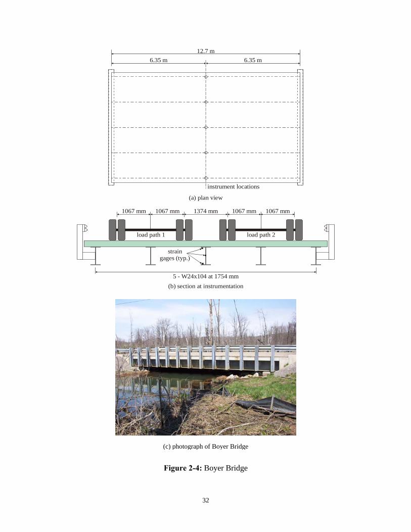
(a) plan view

instrument locations

5 - W24x104 at 1754 mm

straingages (typ.)

(b) section at instrumentation

1067 mm 1067 mm 1374 mm 1067 mm 1067 mm

12.7 m6.35 m 6.35 m

load path 1 load path 2

(c) photograph of Boyer Bridge

Figure 2-4: Boyer Bridge

32

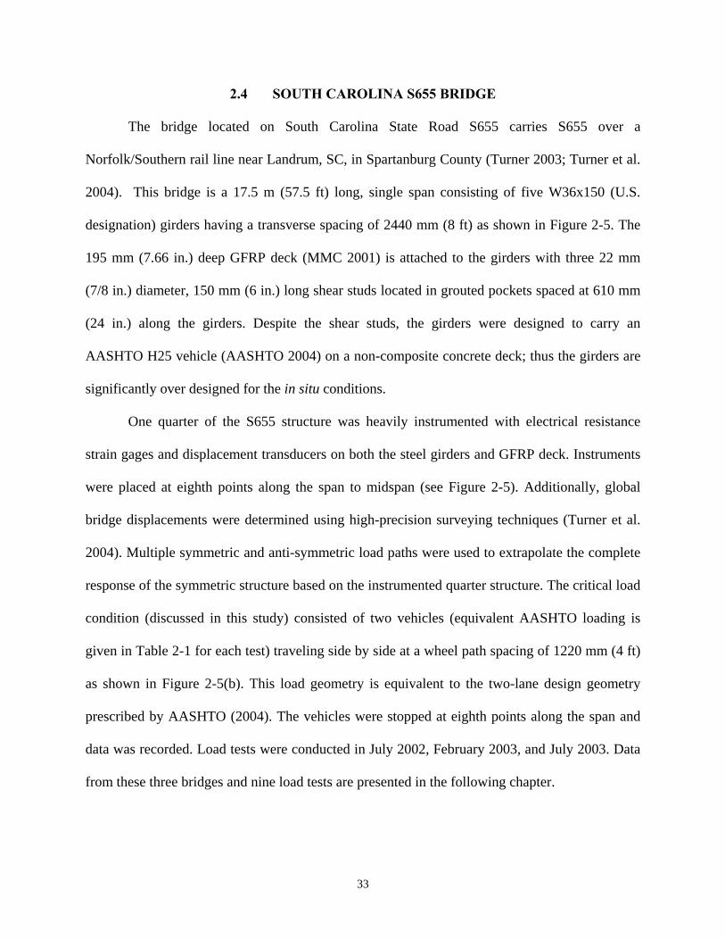
2.4 SOUTH CAROLINA S655 BRIDGE

The bridge located on South Carolina State Road S655 carries S655 over a

Norfolk/Southern rail line near Landrum, SC, in Spartanburg County (Turner 2003; Turner et al.

2004). This bridge is a 17.5 m (57.5 ft) long, single span consisting of five W36x150 (U.S.

designation) girders having a transverse spacing of 2440 mm (8 ft) as shown in Figure 2-5. The

195 mm (7.66 in.) deep GFRP deck (MMC 2001) is attached to the girders with three 22 mm

(7/8 in.) diameter, 150 mm (6 in.) long shear studs located in grouted pockets spaced at 610 mm

(24 in.) along the girders. Despite the shear studs, the girders were designed to carry an

AASHTO H25 vehicle (AASHTO 2004) on a non-composite concrete deck; thus the girders are

significantly over designed for the in situ conditions.

One quarter of the S655 structure was heavily instrumented with electrical resistance

strain gages and displacement transducers on both the steel girders and GFRP deck. Instruments

were placed at eighth points along the span to midspan (see Figure 2-5). Additionally, global

bridge displacements were determined using high-precision surveying techniques (Turner et al.

2004). Multiple symmetric and anti-symmetric load paths were used to extrapolate the complete

response of the symmetric structure based on the instrumented quarter structure. The critical load

condition (discussed in this study) consisted of two vehicles (equivalent AASHTO loading is

given in Table 2-1 for each test) traveling side by side at a wheel path spacing of 1220 mm (4 ft)

as shown in Figure 2-5(b). This load geometry is equivalent to the two-lane design geometry

prescribed by AASHTO (2004). The vehicles were stopped at eighth points along the span and

data was recorded. Load tests were conducted in July 2002, February 2003, and July 2003. Data

from these three bridges and nine load tests are presented in the following chapter.

33

(a) plan view

instrument locations

5 - W36x150 at 2440 mm

straingages (typ.)

(b) section at instrumentation

1830 mm 1220 mm 1830 mm

17.5 m

4 spaces at 2185 mm

single, two vehicleload case

(c) photograph of South Carolina SC655 Bridge

Figure 2-5: South Carolina SC655 Bridge

34

3.0 OBSERVED RESULTS OF LOAD TESTS

Complete results from all load tests are reported in their respective source references

(BDI 2003; Luo 2003; Turner 2003). The present study reports derived behavior parameters for

only the critical elements and critical load tests (see Chapter 2) conducted on each structure. It is

the objective of the following sections to place these parameters – the apparent effective width of

the GFRP deck and the apparent moment distribution factors – in the context of current

AASHTO requirements for steel girder bridges having reinforced concrete decks.

3.1 APPARENT EFFECTIVE WIDTH

The apparent effective width of GFRP deck participating in resisting longitudinal flexure

in a composite manner with the steel girders is calculated for each bridge in the same manner.

The vertical location of the neutral axis of the steel girder resisting the applied vehicle load is

determined from at least two strain measurements taken over the depth of the girder. In all cases,

the neutral axis was found to be located higher in the section than the mid-depth of the steel

beam (which would be the location of the neutral axis if no composite action was present).

Knowing the material properties and geometry of the GFRP deck and steel beam, the effective

width contributing to the flexural resistance (and thus resulting in the change in neutral axis

location) can be calculated for the composite section (see Chapter 1.3.1.1). In this calculation,

the effective width is calculated assuming both top and bottom GFRP face plates contribute

equally. A sample apparent effective width calculation for the interior girder of the Boyer Bridge

(test 1) is given in Appendix A. The inherent assumptions of this procedure are that all strains are

35

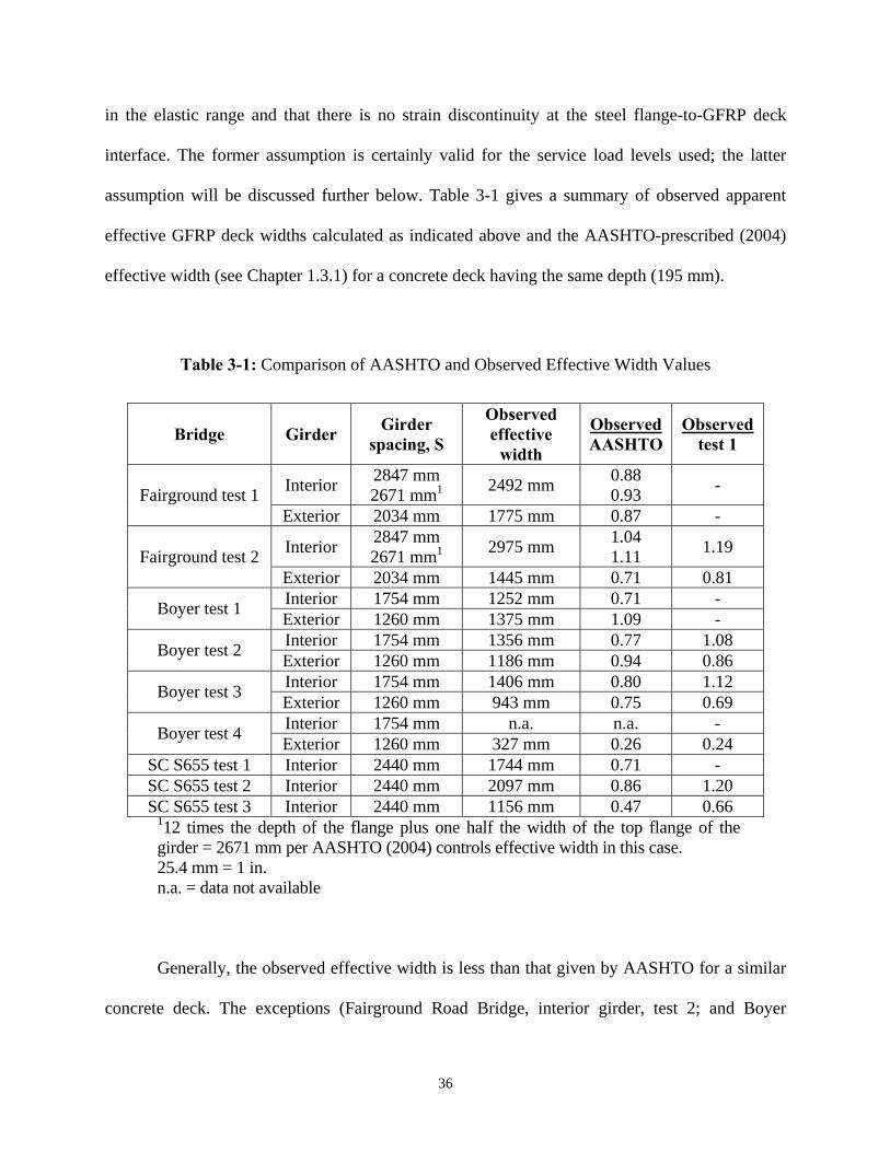
in the elastic range and that there is no strain discontinuity at the steel flange-to-GFRP deck

interface. The former assumption is certainly valid for the service load levels used; the latter

assumption will be discussed further below. Table 3-1 gives a summary of observed apparent

effective GFRP deck widths calculated as indicated above and the AASHTO-prescribed (2004)

effective width (see Chapter 1.3.1) for a concrete deck having the same depth (195 mm).

Table 3-1: Comparison of AASHTO and Observed Effective Width Values

Bridge Girder Girder spacing, S

Observed effective

width

Observed AASHTO

Observed test 1

Interior 2847 mm 2671 mm1 2492 mm 0.88

0.93 - Fairground test 1 Exterior 2034 mm 1775 mm 0.87 -

Interior 2847 mm 2671 mm1 2975 mm 1.04

1.11 1.19 Fairground test 2 Exterior 2034 mm 1445 mm 0.71 0.81 Interior 1754 mm 1252 mm 0.71 - Boyer test 1 Exterior 1260 mm 1375 mm 1.09 - Interior 1754 mm 1356 mm 0.77 1.08 Boyer test 2 Exterior 1260 mm 1186 mm 0.94 0.86 Interior 1754 mm 1406 mm 0.80 1.12 Boyer test 3 Exterior 1260 mm 943 mm 0.75 0.69 Interior 1754 mm n.a. n.a. - Boyer test 4 Exterior 1260 mm 327 mm 0.26 0.24

SC S655 test 1 Interior 2440 mm 1744 mm 0.71 - SC S655 test 2 Interior 2440 mm 2097 mm 0.86 1.20 SC S655 test 3 Interior 2440 mm 1156 mm 0.47 0.66

112 times the depth of the flange plus one half the width of the top flange of the girder = 2671 mm per AASHTO (2004) controls effective width in this case. 25.4 mm = 1 in. n.a. = data not available

Generally, the observed effective width is less than that given by AASHTO for a similar

concrete deck. The exceptions (Fairground Road Bridge, interior girder, test 2; and Boyer

36

Bridge, interior girder, test 1) likely reflect errors in the recorded data since the calculated

effective width is greater than the girder spacing.

The discrete, rather than continuous nature of the shear connection for a GFRP deck,

appears to contribute to the reduced efficiency of the deck. The Boyer Bridge, which had fewer

shear studs at each connection (two, rather than three) and a smaller girder spacing has an

apparent effective width of about 1300 mm (75% of that of an equivalent concrete deck). For the

Fairground and SC S655 bridges, both having three studs per connection, the apparent effective

widths were on the order of 2500 mm and 1665 mm, respectively - approximately 80% of that of

an equivalent concrete deck. These results are consistent with the reduced shear connection

capacities reported previously for similar three-stud connections (Moon et al. 2002; Turner et al.

2003). Similarly the reduction apparent in the Boyer Bridge is consistent with shear connection

capacities reported for similar two-stud connections (Yulismana 2005). Shear lag resulting from

the relatively small grouted pocket (as compared to the larger deck panel) will also affect this

behavior and result in a smaller effective width. Finally, as demonstrated by Keller et al. (2004),

the GFRP deck type used in this study has relatively low in-plane shear stiffness, affecting the

ability to fully engage the top face plate as described in Chapter 1.3.2.2.

The impact of the reduced effective width is to increase the stress level carried by the

steel girder. Compounding this effect is the fact that the GFRP deck is not as axially stiff as a

concrete deck in the first place and will therefore contribute less to composite action in any

event.

Also evident in the final column of Table 3-1 is an apparent degradation in available

composite action, particularly for exterior girders, as measured by a decrease in apparent

effective width over time. In this regard, a thorough inspection of the flange-haunch-deck

37

interface of the SC S655 Bridge did not reveal any obvious degradation or interface cracks

although all strain and deflection data collected revealed the same significant degradation

indicated in Table 3-1 (Turner 2003).

3.2 MOMENT DISTRIBUTION FACTORS FROM IN-SITU TESTS

Moment distribution factors were derived from girder strain data and calculated using

Equation 1.5. For the SC S655 Bridge, symmetry was assumed in order to obtain strains from the

uninstrumented girders (Turner 2003). Confidence in this assumption was developed in two

ways. First, similar calculations were made by superimposing symmetric and anti-symmetric

load cases (Turner 2003) resulting in similar results for a less critical load case. Secondly,

moment distribution calculations based on girder strains and girder deflections yielded uniform

results (Turner 2003).

Table 3-2 reports observed moment distribution factors as well as those calculated using

standard AASHTO practices. The first column of the table gives the bridge and test number. The

second and third columns show the distribution factors calculated according to AASHTO LRFD

(2004) and AASHTO Load Factor Design (1996) given in Eq. 1.3 and Eq. 1.4, respectively. The

fourth and fifth columns show the distribution factors calculated using the lever rule using both

AASHTO-prescribed (2004) load placement (to cause the greatest girder reactions) and the

actual load placement from each test (See Figures 2-3 through 2-5). The sixth column of the

table shows the value of the moment distribution factor observed from in-situ field tests

calculated based on Equation 1.5. The final four columns of the table show the ratio of the

observed value to each of the theoretical values.

38

Table 3-2: Comparison of AASHTO and Observed Moment Distribution Factor Values

Moment Distribution Factor Ratio of observed value to…

AASHTO Lever Rule Bridge

(2004) EQ 1.3

(1996) EQ 1.4

AASHTO prescribed geometry

based on geometry shown in

Figs 2.3-2.5

Observed (2004) EQ 1.3

(1996) EQ 1.4

AASHTO prescribed geometry

based on geometry shown in

Figs 2.3-2.5

Fairground 1 0.864 0.651 0.86 0.77 0.68 0.75 Fairground 2 0.756 0.848 0.964 0.738 0.676 0.89 0.80 0.70 0.78

Boyer 1 0.536 1.01 1.02 0.82 0.88 Boyer 2 0.501 0.94 0.96 0.77 0.82 Boyer 3

0.532 0.523 0.653 0.609 0.523 0.98 1.00 0.80 0.86

SC S655 1 0.876 1.27 1.20 1.00 1.17 SC S655 2 0.811 1.18 1.12 0.93 1.08 SC S655 3

0.688 0.727 0.875 0.750 0.777 1.13 1.07 0.89 1.04

Moment distribution factors are calculated from test results and are affected by the

geometry of the load vehicle and load path used. In the cases of the Fairground and Boyer

bridges the following discrepancies from AASHTO-prescribed geometry were present and are

believe to affect the calculated values of distribution factor to some extent:

1. The gages (axle width) of the test vehicles (see Figures 2-3 and 2-4) were larger than the

1830 mm (72 in.) prescribed by AASHTO. Zokaie et al. (1992) report that experimentally

observed distribution factors will be lower when the test vehicle gage is larger than that

used to calibrate the AASHTO guidelines. This effect may be evident in the Fairground

Road Bridge data where the truck gage in test 2, although still larger than 1830 mm, was

smaller than that used in test 1.

2. In both the Fairground and Boyer bridges, the two-truck load case was determined by

superimposing adjacent load cases each using a single vehicle. Significantly, the resulting

“passing distance” between the trucks was larger, 1372 mm (54 in.), than the AASHTO

39

prescribed, 1220 mm (48 in.). This increased truck spacing will also result in lower

calculated distribution factors (Zokaie et al. 1992).

Therefore, if two vehicles having the correct gage and passing distance were used for the

Fairground and Boyer Bridge load tests, larger observed moment distribution factors than those

reported in Table 3-2 may be expected. The two-truck load case having a 1220 mm (4 ft.)

passing distance used for the SC S655 Bridge (see Figure 2-5) is consistent with the AASHTO

prescribed load case from which moment distribution factors should be calculated.

Considering the forgoing discussion, the observed moment distribution factors for both

the Boyer and SC S655 bridges given in Table 3-2 are greater than the AASHTO-prescribed

values for comparable depth concrete decks. Thus, using the AASHTO values for concrete decks

is unconservative when GFRP decks are used. In both of these cases, the lever rule appears to

give a reasonable and appropriately conservative estimate. The observed values for the

Fairground Bridge appear to be conservative although this result must be understood in the

context of using a loading vehicle having a larger gage and greater passing distance. These

effects are compounded again by the larger girder spacing resulting in relatively conservative

experimental results. Furthermore, it is also acknowledged that AASHTO distribution factors

become more conservative as the girder spacing, S, increases (Eom and Nowak 2001).

The moment distribution factors reported in Table 3-2 appear to reflect the lower

transverse flexural stiffness of a GFRP deck as compared to a concrete deck. The lower stiffness

in the transverse deck direction should result in less redistribution of force beyond adjacent

girders. There is no significant change in the observed distribution factor with the age of the

bridge at testing.

40

3.3 IMPLICATIONS FOR NEW CONSTRUCTION USING GFRP DECKS

The eventual use of GFRP decks for new bridge construction is unclear. Light-weight

GFRP decks are attractive for certain applications such as moving spans (bascules, etc.) and

bridges located in remote areas where placing a concrete deck may become impractical (Moses

et al. 2005). Currently, there are no AASHTO guidelines for the application of GFRP decks and

designers appear to treat these decks as “equivalent to concrete”. Based on the observations

reported in this study, two recommendations for new construction using GFRP decks can be

made:

3.3.1 Composite Behavior

Although a degree of composite behavior is evident at service load levels as described in

Chapter 3.1, the degree of composite action is less than that attainable with an equivalent

concrete deck. Additionally, as discussed in Chapter 1.3.2.1, shear connections between the

GFRP deck and steel girder appear to have limit states associated with failure of the deck and the

full shear capacity may generally not be attained. Therefore, it is proposed that for the purposes

of STRENGTH (AASHTO 2004; see also Chapter 4) design, GFRP decks should not be

assumed to act in a composite manner with steel girders.

For SERVICE (AASHTO 2004; see also Chapter 4) level checks, some composite action

may be present. Based on the results presented, the degree of composite behavior appears to be

less than that attainable by comparable concrete decks and the behavior appears to degrade with

time. Therefore, conservatively, composite action may be neglected. For predictive purposes for

the MMC GFRP deck, an effective width equal to 75% of that calculated for a concrete deck

having the same depth as the GFRP deck (beff, see Chapter 1.3.1) is appropriate for determining

behavior shortly after construction. This value should be reduced to 50% for long-term behavior.

41

The foregoing values are based on the MMC deck tested having two or three studs per

connection located at 610 mm on center.

3.3.2 Moment Distribution Factors

GFRP decks are both longitudinally and transversely more flexible than comparable

concrete decks. There is insufficient data to accurately determine a relationship for the

distribution factors in a form similar to other AASHTO equations. For this reason it is proposed

that moment distribution factors may be best estimated using the lever rule. This formulation is

appropriately conservative as indicated in Chapter 3.2.

3.4 IMPLICATIONS FOR REPLACING CONCRETE DECKS WITH GFRP DECKS

Because of their significantly reduced weight and enhanced durability characteristics,

GFRP decks offer a very attractive alternative for bridge deck replacement, particularly in cases

where the existing bridge superstructure or substructure is structurally deficient. The reduced

dead load of the deck may permit removing posting or increasing the rating of a bridge.

Additionally, GFRP decks may allow similar enhancements for historic bridges without

requiring additional structural retrofit, which may affect the historic fabric of the bridge.

Nonetheless, there are implications of the reduced apparent effective width and increased

distribution factors discussed in the previous sections.

The primary consideration when replacing composite concrete bridge decks using GFRP

decks is that the supporting girders will be required to support increased live load stresses. This

increase results both from the decreased composite action and increased distribution factors

(resulting in decreased transverse distribution of forces). Although the dead load stress will likely

be reduced, the live load stress is transient and thus represents the stress range considered for

42

fatigue sensitive details. This increased stress range must be considered if fatigue-prone details

are present.

The decreased composite action available when a GFRP deck is installed also has the

effect of increasing compressive stresses in the steel girder since the neutral axis is effectively

lower. As such, compression flange and web region stress conditions change and slenderness and

stability effects must be considered.

Current practice is generally to assume that no composite action between a GFRP deck

and steel girder is available and that the girders must resist flexural loads in a non-composite

manner. The results of the present study support this practice. Particularly the apparent

degradation in composite action (as measured by effective deck width given in Table 3-1) over

the course of only a few years in the Boyer and SC S655 bridges indicates that composite action

should not be considered for the STRENGTH (AASHTO 2004) load cases when GFRP decks

are used to replace concrete decks, regardless of the original structural condition. Similar to the

discussion in Chapter 3.3.1, composite action may be considered for SERVICE (AASHTO 2004)

load checks, although the composite action will be significantly reduced from that of a

comparable concrete deck and may be conservatively neglected altogether.

Distribution factors may also increase when a GFRP deck is used in place of a concrete

deck. This increase results in girders adjacent the wheel paths carrying proportionally greater

loads than would be the case were a concrete deck used. The implication of this in existing

structures is that, once again, stress levels in the girders will increase. Bridge geometry (girder

spacing and location of girders relative to travel lanes) will have a significant influence on this

effect. Similar to new construction, use of the lever rule to determine distribution factors is

appropriately conservative for GFRP decks.

43

4.0 ILLUSTRATIVE EXAMPLE – SUPERSTRUCTURE STRESSES

In a bridge deck replacement scenario, a concrete deck may be replaced with a GFRP

deck. The original concrete deck may be composite with the underlying steel girders or non-

composite. Similarly, the GFRP deck may be composite or non-composite. Certainly by

replacing a concrete deck with a GFRP deck, the structural weight (dead load) is reduced.

Nonetheless, as a result of the observed decreased composite action and the increased

distribution factors discussed in Chapter 3, the resulting stresses in the supporting girders may

increase. As will be shown in the following sections, this is particularly the case for the

compression flange of the supporting girder. The magnitude of live loads are unaffected by the

deck replacement. Again, however, resulting live load transient stresses in the supporting girders

are increased due to the reduced composite action and the increased distribution factors. This

increased stress range must be considered if fatigue-prone details are present. The following

sections present an illustrative example, based on the geometry of the South Carolina SC655

Bridge, which assesses girder stresses prior to and after the replacement of an existing concrete

deck.

4.1 PROTOTYPE BRIDGE SECTIONAL PROPERTIES

Table 4-1 lists material properties and resulting member properties for a single interior

girder for the example bridge. The example is based on the SC655 Bridge (Turner et al. 2004)

reported in Section 2.4. Four cases were considered in evaluating the stress range and live load

44

capacity of the example bridge. The first case represents a 216 mm (8.5 in.) thick concrete deck

acting compositely with the underlying W36x150 steel girders. Case 2 represents the same 216

mm (8.5 in.) concrete deck acting in a non-composite manner. The third case represents a 195

mm (7.66 in.) thick MMC GFRP deck acting compositely with the underlying girders. The

fourth case represents the same 195 mm (7.66 in.) thick GFRP deck acting non-compositely with

the underlying girders. All cases had a 25 mm (1 in.) thick grout haunch between the deck soffit

and girder.

As a point of clarification, the S655 Bridge was not a deck replacement. The designers of

the S655 Bridge assumed the behavior to be represented by Case 3: the GFRP deck acting

compositely with the girders. Nonetheless, the girders are detailed to satisfy the requirements of

Case 2 in the event that the GFRP deck needed to be replaced. In South Carolina, such a rapid

deck replacement would be carried out using a precast concrete deck and no composite action

would be provided for.

45

Table 4-1: Material and Member Properties

Material Properties Case 1 - Concrete Composite

Case 2 - Concrete Non-composite

Case 3 - GFRP Composite

Case 4 - GFRP Non-Composite

Deck wt., kPa (psf) 5.081 (106) 5.081 (106) 0.962 (20) 0.962 (20) Esteel, GPa (ksi) 200 (29,000) 200 (29,000) 200 (29,000) 200 (29,000)

Egrout, GPa (ksi) 3 24.9 (3,605) 24.9 (3,605) 24.9 (3,605) 24.9 (3,605) Econcrete, GPa (ksi) 3 24.9 (3,605) 24.9 (3,605) N/A N/A

EFRP, GPa (ksi)2 N/A N/A 13.3 (1,923) 13.3 (1,923) n1 = Esteel/EFRP N/A N/A 15.1 15.1

n2 = Esteel/Egrout = Esteel/Econcrete 8.0 8.0 8.0 8.0 beff, mm (in) 2,438 (96) 2,438 (96) 0.75 x 2438 = 1,829 (72) 0.75 x 2438 = 1,829 (72)

DF 0.688 (Eq. 1.3)

0.688 (Eq. 1.3)

0.875 (lever rule)

0.875 (lever rule)

Member Properties Ix (Itr for composite), mm4 (in4) 1.09x1010 (26,260) 3.76x1010 (9,040) 5.13x1010 (12,332) 3.76x1010 (9,040)

Mp, kN·m (kip·ft) 6,018 (4,438) 3,283 (2,421) 5,028 (3,690) see Section 4.1.1 3,283 (2,421)

ytop, mm (in) 44 (1.74) 456 (17.95) 372 (14.66) 456 (17.95) ybot, mm (in) 868 (34.16) 456 (17.95) 540 (21.24) 456 (17.95)

1 density of concrete assumed to be 2400 kg/m3 (150 pcf) 2 Turner et al. (2004) 3 calculated per ACI (2005) based on fc’ = 27.6 MPa (4,000 psi); grout and concrete assumed to be the same material

For the composite cases, Case 1 and Case 3, composite section properties were derived

using simple mechanics (See Figs. 4.1-2). For Case 1, the neutral axis of the composite section

was calculated using an effective width for the concrete slab of 2,438 mm (96 in.), equal to the

girder spacing. For Case 3, as recommended in Section 3.4, an effective width of 75% of the

Case 1 value, or 1829 mm (72 in.) was used. The distribution factor (Table 4-1) used for

subsequent load calculations was determined from Eq. 1.3 for the concrete decks (Cases 1 and 2)

and using the lever rule, as recommended in Section 3.4, for the GFRP decks (Cases 3 and 4).

Both the grout haunch and concrete deck were assumed to have a compressive strength, fc’, of

27.6 MPa (4,000 psi). The reported compressive strength of the GFRP deck was 172.4 MPa (25

ksi) and the compressive failure strain was 0.013 (Turner et al. 2004), resulting in a compressive

46

modulus, EFRP equal to 13.3 GPa (1,923 ksi) (Table 4-1). Once the neutral axis was located, the

transformed moment of inertia for the composite section was calculated. This process is

tabulated in Appendix B-1 Tables B-1 & B-2.

47

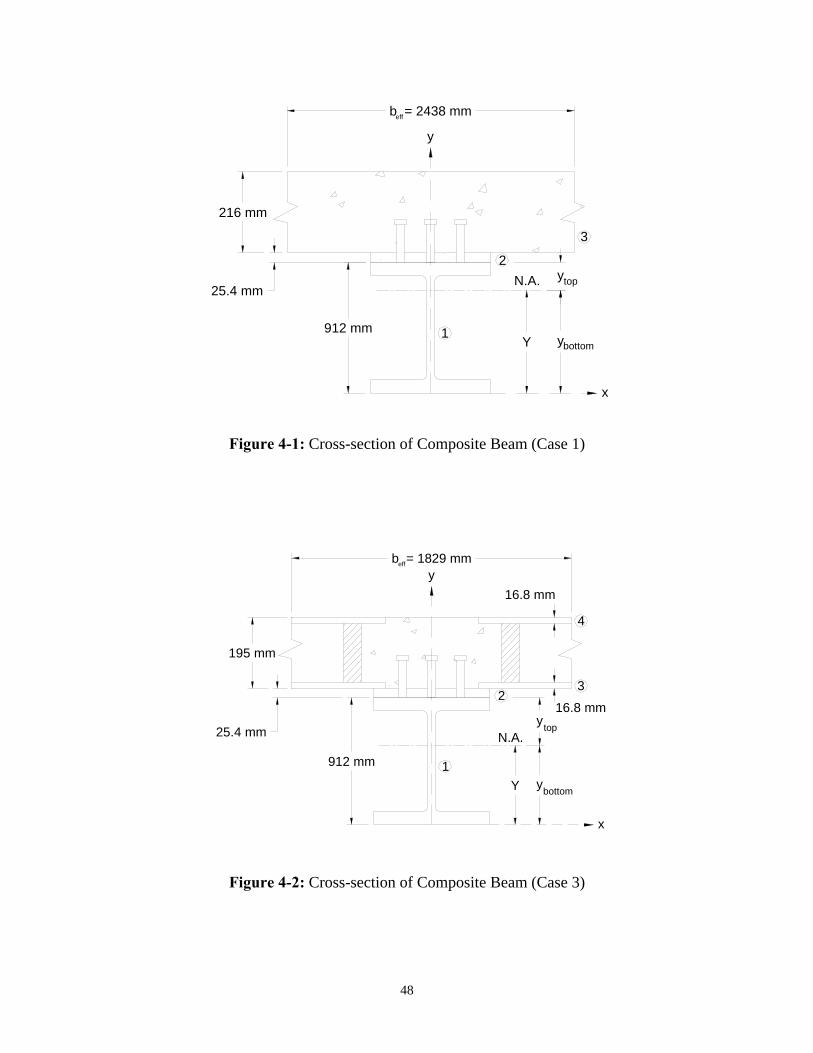
912 mm

25.4 mmy

Y y

x

N.A.

1bottom

top

b = 2438 mm

216 mm

eff

2

3

y

Figure 4-1: Cross-section of Composite Beam (Case 1)

16.8 mm

912 mm

25.4 mmy

1Y y

x

bottom

N.A.top

b = 1829 mm

195 mm

eff

y16.8 mm

23

4

Figure 4-2: Cross-section of Composite Beam (Case 3)

48

The plastic moment capacity, Mp, for the non-composite cases, Cases 2 & 4, was simply

calculated by multiplying the plastic section modulus of the W36 beam, Zx, by the yield stress of

the beam, Fy. This yielded a value for plastic moment capacity of 3,283 kN·m (2,421 kip·ft) for

Cases 2 & 4 (See Table 4-1). The calculation of plastic moment capacity for the composite cases

was a little more involved. For Case 1, the location of the plastic neutral axis (PNA) was

determined in the traditional manner for steel-concrete composite sections, assuming the

Whitney rectangular stress distribution applied to the slab cross section and a critical concrete

strain of 0.003. For Case 1, the value of the plastic moment capacity was determined to be 6,018

kN·m (4,438 kip·ft) (See Table 4-1). The aforementioned calculations are shown in App. B-1.

4.1.1 Plastic Moment Calculation for Composite GFRP Case

The calculation of plastic moment capacity is further complicated for Case 3. Because

GFRP behaves in a linear elastic manner to failure, the compressive stress in the bottom face

sheet of the GFRP deck does not equal the compressive stress in the top face sheet. Rather the

stress distribution through the deck reflects the assumed linear strain distribution. In order to

determine the section capacity, the strain in the top face sheet is assumed to be at its ultimate

value (see calculations below). The PNA is then selected and the stresses through the section are

calculated and the net axial force on the section is determined. The location of the neutral axis is

iterated upon until the net axial force equals zero. And thus the PNA, corresponding to the peak

GFRP strain, is determined and the corresponding plastic moment capacity may be calculated.

The GFRP face sheets are relatively thin and the top face sheet is only supported at

discrete lines (the webs) perpendicular to the applied compressive stress field. Therefore,

buckling of the top face plate is possible. Thus, before continuing the calculation of the plastic

moment capacity, the ultimate compressive stress of the top face sheet (and thus, the

49

corresponding strain) must be determined accounting for the effective length between web

supports. The top face sheet is supported by the deck webs at alternating spacings of 170 (5.7 in.)

and 135 mm (5.3 in.) (see Figure 2-1). For the purposes of this calculation, the longer effective

length is used.

The loading geometry of the top face sheet is shown in Figure 4-3. The choice of the

width of the section, b, is not relevant since, in the calculation of AIr /= , the b terms cancel.

The critical buckling stress is calculated as:

( )22

rkL

Ecr

πσ = (4.1)

b

135 mm

170 mm

t = 16.8 mm

Figure 4-3: Loading Condition of Top Face Plate

Although it is slightly conservative, the webs are assumed to only provide a “simple”

support; therefore, the value of k = 1 is selected. Solving Equation 4.1, the critical stress for the

top plate may be found to 105.5 MPa (15.3 ksi). The corresponding ultimate strain is 0.008. This

latter value is used as the top face sheet strain in the determination of the plastic capacity of the

composite GFRP deck section (Case 3).

50

The strain at the bottom face sheet is denoted by εb and the plastic neutral axis is denoted

as y in Fig. 4-4. The stresses for each section were arrived at by utilizing Hooke’s Law,

εσ ⋅= E . The forces at each section were then found by multiplying the stress by the cross

sectional area. All forces above the PNA are compressive forces, and all forces below the PNA

are tensile forces.

11.9

(y - 23.9) / 2

y + (912 - y - 23.9)/2900946

1123

y (mm)

y

7,290 2,509

Eccentricity, e = y - y

yσ·A15.9*(912 - y - 23.9)

15.9*(y - 23.9) σ·Ay

7,29030,645

30,645

13,261·ε·(A)2,509

b

3,234 0.008

εb

A (mm ) Force (kN)2

Figure 4-4: Determination of Plastic Section

As a sample calculation, illustrated in Figure 4-4, assume that the plastic neutral axis is

762 mm (30 in.) above the base of the steel beam, i.e. y = 762 mm. The top face sheet strain is

set at 0.008 which corresponds to a value of εb = 0.004. The compressive force in the top face

sheet is then:

( ) ( ) ( ) kNMPammmmA 32345.10576.161829 =⋅⋅=⋅σ

The compressive force in the bottom face sheet is:

( ) ( ) ( ) kNGPammmmEA b 628,1004.026.1376.161829 =⋅⋅⋅=⋅⋅ ε

51

The compressive force in the top flange of the steel member (whose strain is 0.003) is:

( ) ( ) ( ) kipsMPammmmA 25097.34424305 =⋅⋅=⋅σ

Similarly, the tensile force at the bottom flange of the steel member is:

( ) ( ) ( ) kNMPammmmA 25097.34424305 =⋅⋅=⋅σ

At this point in the calculation, it can be seen that the net axial force on the section will

be compressive since the web is only able to provide 4,804 kN (1,080 kips) if it is acting entirely

in tension (which it is not in this sample calculation). Thus the selection of the PNA, y = 762 mm

(30 in.) is too low. A new value for the PNA is selected and the calculations repeated until the

net axial force on the section is equal to zero.

Through trial and error, the location of the PNA is found to be y = 856 mm (33.7 in.).

The plastic moment capacity for the section can then be calculated by taking a summation of the

force components multiplied by their distance to the PNA (See Table 4-2). This results in a

plastic moment capacity of 5,030 kN·m (3,690 kip·ft). As expected, this value lies between the

non-composite capacity of the W36x150 alone (Cases 2 and 4) and the composite capacity

calculated assuming a stiffer concrete deck (Case 1).

Table 4-2: Plastic Moment Capacity Calculation

Force, F

kN (kips) Eccentricity, e

mm (in) F*e - kN·m (kip·ft)

Top face sheet 3,234 (727) 267.5 (10.53) 864.9 (637.9) Bottom face sheet 1,112 (250) 89.7 (3.53) 99.7 (73.5) Top flange steel 2,509 (564) 43.9 (1.73) 110.2 (81.3) Web (Comp.) 191 (43) 17.3 (0.68) 3.3 (2.4)

Steel Web (Tens.) -4,541 (-1,021) -414.8 (-16.33) 1,883.7 (1,389.4) Bottom flange steel -2,509 (-564) -823.7 (-32.43) 2,066.4 (1,524.2)

≈ 0 5,028.3 (3,708.9)

52

4.2 APPLIED LOADING AND LOAD CASES

Complete load calculations are presented in Appendix B-2. The loads applied to the

structure were determined based on the 2004 AASHTO LRFD Specification. The prescribed

dead loads: DC, the load due to bridge components and DW, the load due to the wearing surface

(assumed to be 38 mm (1.5 in.) of asphalt overlay), were calculated and distributed evenly to

each of the five supporting girders. From these uniformly distributed loads, the maximum dead

load moments were calculated. The live load (LL) was based on AASHTO H25 design loading.

The load was placed longitudinally on the span to yield the maximum live load moment (see

Appendix B-2). The distribution factors (DF) given in Table 4-1 are applied to all live load cases.

Three AASHTO load cases are considered: STRENGTH I, SERVICE I and FATIGUE

(AASHTO 2004 – Table 3.4.1-1). The load combinations and resulting design moments for an

interior girder are presented in Table 4-3. As an illustrative example, only the interior girders are

considered in this discussion.

53

Table 4-3: Design Loading and Moments (see Appendix B-2 for details)

Loading Cases 1 & 2 - Concrete Deck

Cases 3 & 4 - GFRP Deck

Deck 12.40 (0.850) 2.34 (0.160) Girder 2.19 (0.150) 2.19 (0.150) Parapet 2.38 (0.163) 2.38 (0.163)

Dead Load of Components DC - kN/m (kips/ft)

Diaphragms 0.18 (0.012) 0.18 (0.012)

Dead Load of Wearing Surface

DW - kN/m (kips/ft)

38mm (1.5") Asphalt Wearing Surface

2.19 (0.150) 2.19 (0.150)

Live Load

H25 H25

Moments MDC - kN·m (kip-ft) 658.5 (485.6) 271.8 (200.4) MDW - kN·m (kip-ft) 84.1 (62.0) 84.1 (62.0) MLL - kN·m (kip-ft) 606.9 (447.6) 772.0 (569.3)

STRENGTH I Mu = 1.75(1.33*MLL)+1.25MDC+1.5MDW kN·m (kip-ft) 2,361.9 (1,741.8) 2,262.6 (1,668.6)

SERVICE 1 Mu = 1.00(1.33*MLL)+1.00MDC+1.00MDW kN·m (kip-ft) 1,549.8 (1,142.9) 1,382.6 (1,019.6)

FATIGUE Mu = 0.75(1.15*MLL) kN·m (kip-ft) 523.5 (386.1) 665.8 (491.0)

54

4.3 STRESSES IN STEEL GIRDERS

Once the dead and live load moments were calculated for each case, they were used to

determine the stress in the top and bottom flanges of the W36x150 girders. The stress at the

extreme fibers of the girder is arrived at by using the equation:

xI

My=σ (4.2)

Where, σ = stress at location y

M = applied moment (Table 4-3)

y = distance from neutral axis to extreme fiber (ytop and ybot from Table 4-1)

I = moment of inertia of section (Table 4-1)

Stresses due to dead and live loads, in addition to total stresses were calculated at the

extreme tensile and compressive fibers for each of the three load cases considered. The results

are tabulated in Tables 4-4 through 4-6. In all cases, moments corresponding to DC loads are

applied to the non-composite steel girder section. DW and LL loads are applied to the composite

(Cases 1 and 3) or non-composite (Cases 2 and 4) section as appropriate.

55

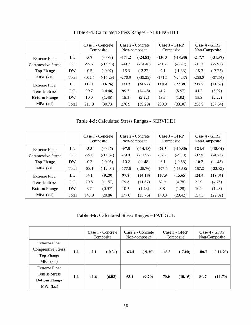
Table 4-4: Calculated Stress Ranges - STRENGTH I

Case 1 - Concrete Composite

Case 2 - Concrete Non-composite

Case 3 - GFRP Composite

Case 4 - GFRP Non-Composite

LL -5.7 (-0.83) -171.2 (-24.82) -130.3 (-18.90) -217.7 (-31.57) DC -99.7 (-14.46) -99.7 (-14.46) -41.2 (-5.97) -41.2 (-5.97) DW -0.5 (-0.07) -15.3 (-2.22) -9.1 (-1.33) -15.3 (-2.22)

Extreme Fiber Compressive Stress

Top Flange MPa (ksi) Total -105.5 (-15.29) -270.9 (-39.29) -171.5 (-24.87) -258.9 (-37.54)

LL 112.1 (16.26) 171.2 (24.82) 188.9 (27.39) 217.7 (31.57) DC 99.7 (14.46) 99.7 (14.46) 41.2 (5.97) 41.2 (5.97) DW 10.0 (1.45) 15.3 (2.22) 13.3 (1.92) 15.3 (2.22)

Extreme Fiber Tensile Stress

Bottom Flange MPa (ksi) Total 211.9 (30.73) 270.9 (39.29) 230.0 (33.36) 258.9 (37.54)

Table 4-5: Calculated Stress Ranges - SERVICE I

Case 1 - Concrete Composite

Case 2 - Concrete Non-composite

Case 3 - GFRP Composite

Case 4 - GFRP Non-Composite

LL -3.3 (-0.47) -97.8 (-14.18) -74.5 (-10.80) -124.4 (-18.04) DC -79.8 (-11.57) -79.8 (-11.57) -32.9 (-4.78) -32.9 (-4.78) DW -0.3 (-0.05) -10.2 (-1.48) -6.1 (-0.88) -10.2 (-1.48)

Extreme Fiber Compressive Stress

Top Flange MPa (ksi) Total -83.1 (-12.04) -177.6 (-25.76) -107.4 (-15.58) -157.3 (-22.82)

LL 64.1 (9.29) 97.8 (14.18) 107.9 (15.65) 124.4 (18.04) DC 79.8 (11.57) 79.8 (11.57) 32.9 (4.78) 32.9 (4.78) DW 6.7 (0.97) 10.2 (1.48) 8.8 (1.28) 10.2 (1.48)

Extreme Fiber Tensile Stress

Bottom Flange MPa (ksi) Total 143.9 (20.86) 177.6 (25.76) 140.8 (20.42) 157.3 (22.82)

Table 4-6: Calculated Stress Ranges – FATIGUE

Case 1 - Concrete

Composite Case 2 - Concrete

Non-composite Case 3 - GFRP

Composite Case 4 - GFRP Non-Composite

Extreme Fiber Compressive Stress

Top Flange MPa (ksi)

LL -2.1 (-0.31) -63.4 (-9.20) -48.3 (-7.00) -80.7 (-11.70)

Extreme Fiber Tensile Stress

Bottom Flange MPa (ksi)

LL 41.6 (6.03) 63.4 (9.20) 70.0 (10.15) 80.7 (11.70)

56

There are some important aspects to consider when looking at the theoretical stresses.

First and foremost, the stresses computed for Case 1 are assuming original conditions. It is

unlikely that a perfectly functioning composite concrete deck is going to be replaced. Bridge

decks that are in need of replacement are generally in poor condition. There can be a number of

issues that cause pre-replacement stresses to vary considerably from the theoretical values. For

instance, there can be significant section loss to the steel girders due to deterioration. The deck

may be heavily damaged and heavy spalling of the concrete deck can occur, which decreases the

deck sectional area and can decrease the degree of composite behavior of the girder-deck system.

In an extreme case, a concrete deck designed to act compositely with the underlying stringers

may actually exhibit behavior similar to a non-composite situation.

57

4.4 RETROFIT SCENARIOS

In practice, the following retrofit scenarios are possible:

Scenario A: Composite concrete deck replaced w/ composite GFRP deck – Case 1 to Case 3.

Scenario B: Composite concrete deck replaced w/ non-comp. GFRP deck – Case 1 to Case 4.

Scenario C: Non-comp. concrete deck replaced w/ non-comp. GFRP deck – Case 2 to Case 4.

Scenario D: Non-comp. concrete deck replaced w/ composite GFRP deck – Case 2 to Case 3.

Scenario E: Concrete deck replaced with concrete deck (composite or non-composite).

Scenario E is beyond the scope of the present discussion and will not be considered

further. Scenario A is the case typically considered for concrete deck replacement when GFRP

decks are to be used. Scenario B, on the other hand, is the scenario recommended in the present

work since it is proposed that composite action cannot be fully developed (see Section 3.4).

Scenario C may occur in practice when the concrete deck to be replaced is non-composite with

its supporting members. This may be the case when replacing a concrete deck supported on floor

beams spanning between main girders. Finally, Scenario D is unlikely in practice and will not be

considered further in this discussion. Table 4-7 shows the ratios of girder stresses following deck

replacement to those prior to deck replacement for Scenarios A, B, and C.

58

Table 4-7: Ratios of Post-Retrofit Stresses to Pre-Retrofit Stresses

Retrofit Scenario A B C (Case 1-3) (Case 1-4) (Case 2-4)

Compressive Stresses

STRENGTH I 1.63 2.46 0.96 SERVICE 1 1.29 1.89 0.89 FATIGUE 22.821 38.111 1.27

Tensile Stresses STRENGTH I 1.09 1.22 0.96 SERVICE 1 0.98 1.09 0.89 FATIGUE 1.68 1.94 1.27

1 ratio is misleading due to very small denominator (see Table 4.6)

It is often assumed, incorrectly, that composite concrete bridge decks replaced by GFRP

bridge decks remain fully composite (Scenario A). This fully composite behavior may be

exhibited for SERVICE I and FATIGUE load cases. Nonetheless, as discussed in Section 3.4, it

is unlikely that composite behavior (Case 3) may be achieved for STRENGTH I. Therefore, it is

more appropriate and more conservative to assume non-composite behavior (Case 4) and thus

retrofit Scenario B. As a result there is an error associated with stresses determined assuming

Scenario A when Scenario B is actually appropriate. In this example, compression flange stresses

are underestimated by 34% and tension flange stresses by 11% under STRENGTH I and 32%

and 10% under SERVICE I load combinations. FATIGUE stresses are underestimated by 13%.

Due to the significantly reduced dead load of a GFRP deck (DL stresses are reduced by

more than half in the example shown), Scenario C, when appropriate, results in reduced stresses

on the structure. Although it is noted that Scenario C does have an increased fatigue stress range

due to the increased DF used.

59

4.5 AASHTO FATIGUE CRITERIA

Fatigue loading is a special case and requires particular attention if fatigue-prone details

are present. The following discussion addresses the fatigue requirements from AASHTO (2004).

Fatigue is defined as a member’s tendency to fail at a level of stress below its specified yield

stress when subjected to repeated loading. Fatigue cracking generally results from repeated load

applications and the resulting cyclic stresses, which result from either a long exposure time or a

high frequency of occurrence. Steel cracking and the failures developed as a result of cyclic

loading generally show little or no evidence of plastic deformation. Hence, it is often difficult to

identify these problems before serious damage or failure occurs in the member (FHWA 2003).

Structural details have different levels of resistance to fatigue cracking. Three key factors

affecting the fatigue life of a member are:

• Stress Range (S)

• Number of cycles (N)

• Type of Detail

For the example structure, the FATIGUE stress ranges are given in Table 4-6. The

number of cycles depends on the roadway carried by the bridge (AASHTO 2004 – Section

6.6.1.2.5). A given detail is defined by assigning it to a category ranging from Category A (best

case having little susceptibility to fatigue damage) to Category E’ (worst case). These categories

are defined in AASHTO (2004) Table 6.6.1.2.5-3. Details sharing the same category usually

have comparable fatigue resistance and similar stress concentrations. During the inspection of

fracture critical members, the assigned fatigue category can be a reminder of which details are

the most critical with respect to fatigue cracking. The categories can also set precedence to which

details need to be addressed first.

60

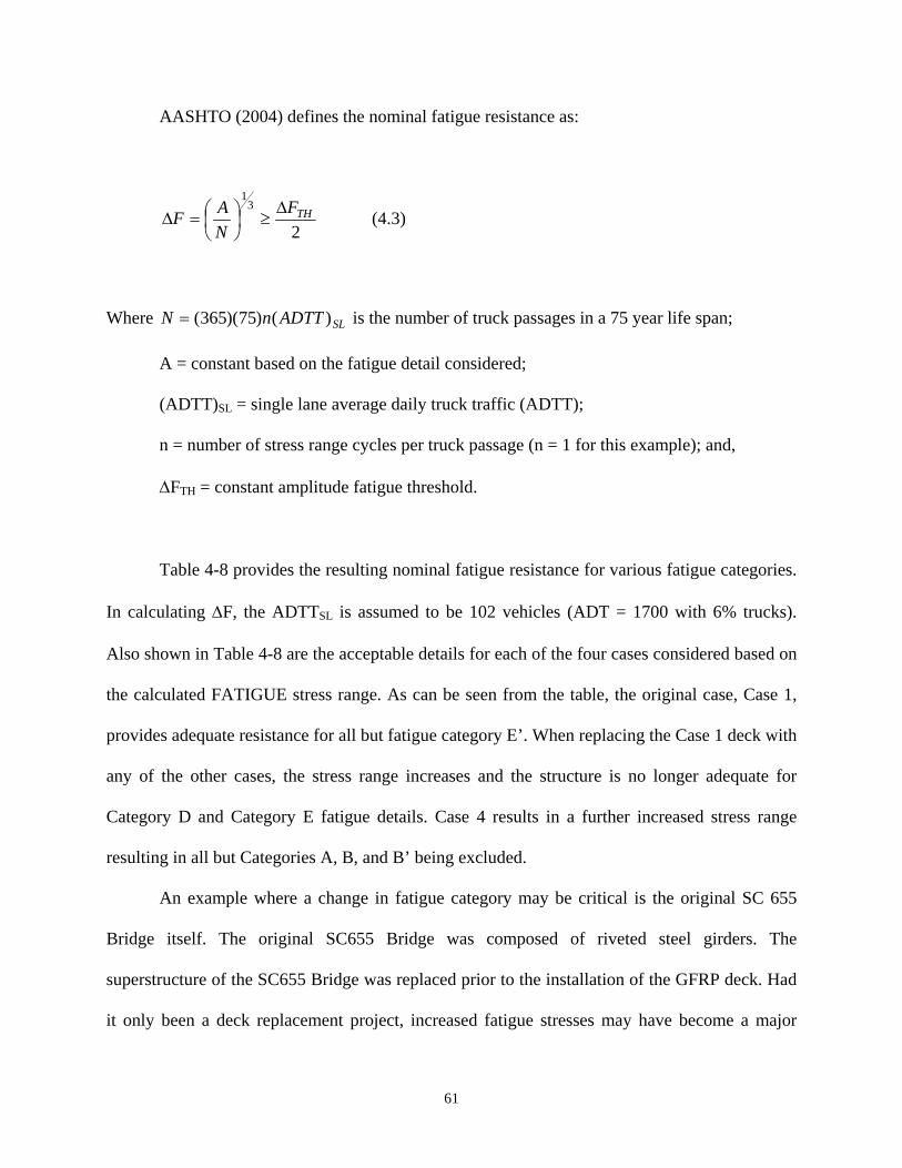
AASHTO (2004) defines the nominal fatigue resistance as:

23

1THF

NAF Δ

≥⎟⎠⎞

⎜⎝⎛=Δ (4.3)

Where is the number of truck passages in a 75 year life span; SLADTTnN )()75)(365(=

A = constant based on the fatigue detail considered;

(ADTT)SL = single lane average daily truck traffic (ADTT);

n = number of stress range cycles per truck passage (n = 1 for this example); and,

ΔFTH = constant amplitude fatigue threshold.

Table 4-8 provides the resulting nominal fatigue resistance for various fatigue categories.

In calculating ΔF, the ADTTSL is assumed to be 102 vehicles (ADT = 1700 with 6% trucks).

Also shown in Table 4-8 are the acceptable details for each of the four cases considered based on

the calculated FATIGUE stress range. As can be seen from the table, the original case, Case 1,

provides adequate resistance for all but fatigue category E’. When replacing the Case 1 deck with

any of the other cases, the stress range increases and the structure is no longer adequate for

Category D and Category E fatigue details. Case 4 results in a further increased stress range

resulting in all but Categories A, B, and B’ being excluded.

An example where a change in fatigue category may be critical is the original SC 655

Bridge itself. The original SC655 Bridge was composed of riveted steel girders. The

superstructure of the SC655 Bridge was replaced prior to the installation of the GFRP deck. Had

it only been a deck replacement project, increased fatigue stresses may have become a major

61

consideration. According to the FHWA, riveted splices are considered a fatigue category D

(FHWA 2003). In this hypothetical example, only Case 1, a composite concrete deck, would

exhibit the necessary fatigue resistance for H25 live loading.

Table 4-8: AASHTO Fatigue Thresholds

AASHTO (2004) Table

6.6.1.2.5-3 Case 1 - Concrete

Composite Case 2 - Concrete

Non-composite Case 3 - GFRP

Composite Case 4 - GFRP Non-Composite

Detail Category

ΔF MPa (ksi) (Eq. 4.3) S = 41.6 (6.03) S = 63.4 (9.20) S = 70.0 (10.15) S = 80.7 (11.70)

A 143.4 (20.8) OK OK OK OK B 112.4 (16.3) OK OK OK OK B' 89.6 (13) OK OK OK OK C 80 (11.6) OK OK OK NG C' 80 (11.6) OK OK OK NG D 63.4 (9.2) OK NG NG NG E 50.3 (7.3) OK NG NG NG E' 35.9 (5.2) NG NG NG NG

62

4.6 SUMMARY

As can be seen in this single illustrative example the internal stresses in the bridge

superstructure are significantly affected when replacing a concrete deck with a GFRP deck. The

more flexible axial behavior of the GFRP deck results in less composite behavior being

developed between deck and superstructure; resulting in a correspondingly lower neutral axis

location. Similarly, the flexible deck does not permit as much transverse distribution of applied

loads resulting in higher loads carried by girders immediate adjacent travel lanes. Finally,

particular care must be taken when replacing the deck on a structure that contains fatigue prone

details. Even though the dead load is reduced when the retrofit employs a GFRP deck replacing a

concrete deck, the live load remains the same. Due to decreased composite action and increased

distribution factors, the resulting live load stresses in the supporting girders may increase. Hence,

this increased stress range must be considered if fatigue-prone details are present.

When a GFRP deck replaces a concrete deck, it has been shown that superstructure

internal stresses may increase; significantly in some cases. Nonetheless, forces on structural

elements further along the load path, i.e. bearings, support bents, abutments, columns, and

foundations, see a reduction in dead load and are relatively unaffected by the composite behavior

of the deck or the distribution factor, which results in a lower stress condition. This may be

significant for certain situations, such as an old bridge that is supported on timber piers.

63

5.0 CONCLUSIONS AND RECOMMENDATIONS

Results from a number of in situ load tests of three steel girder bridges having the same

GFRP deck system were used to examine the degree of composite action that may be developed

and the transverse distribution of wheel loads that may be assumed for such structures. The

following conclusions are made based on the observations of these load tests:

1. In general, the observed effective width is less than that prescribed by AASHTO for a

comparable concrete deck.

2. The discrete, rather than continuous nature of the shear connection for a GFRP deck,

appears to contribute to the reduced efficiency of the deck.

3. There is an apparent degradation in available composite action, particularly for exterior

girders, as measured by a general decrease in apparent effective width over time.

4. The observed moment distribution factors for both the Boyer and SC S655 bridges are

greater than the AASHTO-prescribed values for comparable depth concrete decks.

Current design practice treats GFRP deck systems in a manner similar to concrete decks.

The results of this study indicate that this may result in non-conservative design values for the

bridge girders. Specifically:

5. The effective width of GFRP deck which may be engaged is lower than that of an

equivalent concrete deck. This decrease results from increased horizontal shear lag due to

the less stiff axial behavior of the deck (as compared to concrete) and increased vertical

shear lag due to the relatively soft in-plane shear stiffness of the GFRP deck.

64

6. Increased apparent moment distribution factors, indicating reduced transverse distribution

of wheel loads, are observed due to the increased transverse flexibility of the GFRP deck

system (as compared to an equivalent concrete deck).

5.1 RECOMMENDATIONS

The eventual use of GFRP decks for new bridge construction is unclear. Nonetheless,

light-weight GFRP decks are attractive for certain applications such as moving spans (bascules,

etc.) and bridges located in remote areas where placing a concrete deck may become impractical.

Regardless, the primary application for GFRP decks is thought to be deck replacement. The

following recommendations are focused on the use of GFRP decks for deck replacement

projects.

Because of their significantly reduced weight and enhanced durability characteristics,

GFRP decks offer a very attractive alternative for bridge deck replacement, particularly in cases

where the existing bridge superstructure or substructure is structurally deficient. The reduced

dead load of the deck may, in some cases, permit removing posting or increasing the rating of a

bridge. Additionally, GFRP decks may allow similar enhancements for historic bridges without

requiring additional structural retrofit, which may affect the historic fabric of the bridge.

The primary consideration when replacing composite concrete bridge decks using GFRP

decks is that the supporting girders will be required to support increased live load stresses. This

increase results both from the decreased composite action and increased distribution factors

(resulting in decreased transverse distribution of forces). Although the dead load stress will likely

be reduced, the live load stress is transient and thus represents the stress range considered for

65

fatigue sensitive details. This increased stress range must be considered if fatigue-prone details

are present.

The decreased composite action available when a GFRP deck is installed also has the

effect of increasing compressive stresses in the steel girder since the neutral axis is effectively

lower. As such, compression flange and web region stress conditions change and slenderness and

stability effects must be considered. Composite action should not be considered for the

STRENGTH (AASHTO 2004) load cases when GFRP decks are used in new construction or to

replace concrete decks. Additionally, until significantly more data is made available, the lever

rule should be used to determine distribution factors for GFRP decks. These recommendations

are felt to be appropriately conservative for GFRP decks.

66

APPENDIX A

SAMPLE CALCULATIONS OF BOYER BRIDGE DISTRIBUTION FACTORS AND EFFECTIVE WIDTH

The following calculations are presented in support of the discussion and results presented in

Chapter 3. The calculations are based on the Boyer Bridge presented in Chapter 2.3. All

calculations are based on data obtained from the field test #1 (November, 2001). A ½” grout

haunch was assumed for consistency with Luo (2003).

Properties of the W24x104 girders are given (AISC 2002) as:

d = 24.1 in b = 12.8 in tf = 0.750 in

tw = 0.50 in Ix = 3100 in4

A = 30.6 in2

Zx = 289 in3

Sx = 258 in3

Fy = 50 ksi

67

Boyer Bridge Effective Width Calculation

Haunch, t

t

t

Beam depth, d

h

1Y

x

N.A.fs

beff

yt

4

32

fs

Figure A-1: Cross-section of Composite Beam with GFRP Deck

Table A-1: Effective Width Calculations

Element Area y yA

1 30.60 12.05 368.73

2 8.08

5.08.12=

x 24.35 19.48

3 effeffefffs b

bnbt

057.058.11

66.0== 24.93 1.42beff

4 effeffefffs b

bnbt

057.058.11

66.0== 31.93 1.82beff

Total 31.4+0.114beff 388.2+3.24beff

Equilibrium Equation (31.4+0.114beff) y = 388.2+3.24beff

Observed neutral Axis depth, y 14.80 in.

Calculated Effective Width, beff 49.28 in.

tfs = 0.67 in. th = 0.50 in. t = 7.66 in. d = 24.1 in. ES = 29,000 ksi EFRP = 2,500 ksi n = Ec/EFRP = 11.58

68

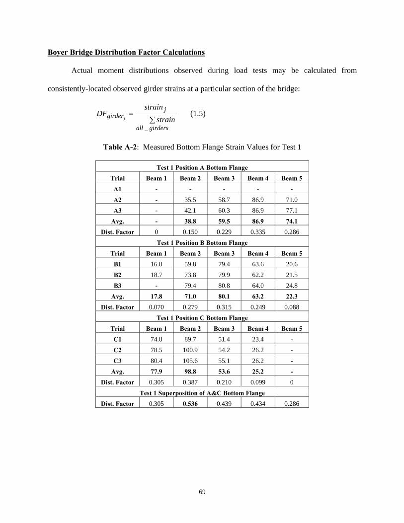
Boyer Bridge Distribution Factor Calculations

Actual moment distributions observed during load tests may be calculated from

consistently-located observed girder strains at a particular section of the bridge:

∑

=

girdersall

jgirder strain

strainDF

j

_

(1.5)

Table A-2: Measured Bottom Flange Strain Values for Test 1

Test 1 Position A Bottom Flange Trial Beam 1 Beam 2 Beam 3 Beam 4 Beam 5 A1 - - - - - A2 - 35.5 58.7 86.9 71.0 A3 - 42.1 60.3 86.9 77.1

Avg. - 38.8 59.5 86.9 74.1 Dist. Factor 0 0.150 0.229 0.335 0.286

Test 1 Position B Bottom Flange Trial Beam 1 Beam 2 Beam 3 Beam 4 Beam 5 B1 16.8 59.8 79.4 63.6 20.6 B2 18.7 73.8 79.9 62.2 21.5 B3 - 79.4 80.8 64.0 24.8

Avg. 17.8 71.0 80.1 63.2 22.3 Dist. Factor 0.070 0.279 0.315 0.249 0.088

Test 1 Position C Bottom Flange Trial Beam 1 Beam 2 Beam 3 Beam 4 Beam 5 C1 74.8 89.7 51.4 23.4 - C2 78.5 100.9 54.2 26.2 - C3 80.4 105.6 55.1 26.2 -

Avg. 77.9 98.8 53.6 25.2 - Dist. Factor 0.305 0.387 0.210 0.099 0

Test 1 Superposition of A&C Bottom Flange Dist. Factor 0.305 0.536 0.439 0.434 0.286

69

APPENDIX B-1

CALCULATIONS OF BRIDGE SECTIONAL PROPERTIES

The following calculations are presented in support of the discussion and results presented in

Chapter 4. The prototype structures are based on the South Carolina S655 bridge presented in

Chapter 2.4. Four cases were selected to represent the bound of behavior:

Case 1: 8.5 inch thick concrete slab on W36 x 150 girders acting in a fully composite manner

Case 2: 8.5 inch thick concrete slab on W36 x 150 girders having no composite action

Case 3: MMC 7.66 inch GFRP deck on W36 x 150 girders acting in a fully composite manner

Case 4: MMC 7.66 inch GFRP deck on W36 x 150 girders having no composite action

Properties of the W36 x 150 girders are given (AISC 2002) as:

d = 35.9 in b = 12.0 in tf = 0.940 in

tw = 0.625 in Ix = 9040 in4

A = 44.2 in2

Zx = 581 in3

Sx = 504 in3

Fy = 50 ksi

70

Case 1: 8.5 inch concrete slab on W36 x 150 girders acting in a fully composite manner Composite Section Properties

8.5"

1.0"y

35.9" 1 yY

x

bottom

N.A. top

b = 96"eff

y

3

2

Figure B-1: Cross-section of Composite Beam with Concrete Deck (Case 1)

Table B-1: Composite Section Properties Calculations for Case 1

Element Area (Transformed) y yA d Ad2 Ix Itr

1 44.2 17.95 793.39 -16.21 11,613 9,040

2 1.5 36.40 54.60 2.24 8 0

3 102.0 41.15 4,197.30 6.99 4,985 614

Total 147.7 5,045.29 16,605 9,654 26,260

Y= 34.16

71

Plastic Moment Capacity Assume plastic neutral axis (PNA) is in slab.

( )( )( )( ) "5.8"77.6

96485.0502.44

'85.0=<==

⋅⋅

= seffc

ys tbf

FAa PNA in slab…OK

( )( )( ) kipsbafC effc 210,29677.6485.0'85.0 ==⋅⋅=

( )( ) kipsFAT ys 210,2502.44 ==⋅=

inattde sgrout 1.24277.65.81

29.35

22=−++=−++=

Plastic Moment Capacity

( )( ) ftkipeCM p ⋅==⋅= 438,412

1.242210

For W36x150: 9.51=wth

9.515.9050000,2976.376.3 =≥==

wy th

FE Mp may be developed…OK

Case 2: 8.5 inch concrete slab on W36 x 150 girders having no composite action and Case 4: MMC 7.66 inch GFRP deck on W36 x 150 girders having no composite action

4040,9 inI x = 3581 inZ x =

ftkipFZM yxp ⋅== 421,2

72

Case 3: MMC GFRP deck on W36 x 150 girders acting in a fully composite manner

Composite Section Properties

7.66"

1.0"y

35.9" 1yY

x

bottom

N.A.top

b = 72"eff

y0.66"

4

3

0.66"

2

Figure B-2: Cross-section of Composite Beam with GFRP Deck (Case 2)

Table B-2: Composite Section Property Calculations for Case 3

Element Area (Transformed) y yA d Ad2 Ix I'x

1 44.2 17.95 793.39 -3.29 478 9,040

2 1.5 36.40 54.60 15.16 345 0

3 3.1 37.23 117.16 15.99 805 0

4 3.1 44.23 139.19 22.99 1,663 0

Total 52.0 1,104.35 3,291 9,040 12,332

Y= 21.24

Plastic Moment Capacity (see Section 4.1.1)

73

APPENDIX B-2

CALCULATIONS OF APPLIED BRIDGE LOADING

The following calculations are presented in support of the discussion and results presented in

Chapter 4. The prototype structures are based on the South Carolina S655 bridge presented in

Chapter 2.4. Four cases were selected to represent the bound of behavior:

Case 1: 8.5 inch thick concrete slab on W36 x 150 girders acting in a fully composite manner

Case 2: 8.5 inch thick concrete slab on W36 x 150 girders having no composite action

Case 3: MMC 7.66 inch GFRP deck on W36 x 150 girders acting in a fully composite manner

Case 4: MMC 7.66 inch GFRP deck on W36 x 150 girders having no composite action

Properties of the W36 x 150 girders are given (AISC) as:

d = 35.9 in b = 12.0 in tf = 0.940 in

tw = 0.625 in Ix = 9040 in4

A = 44.2 in2

Zx = 581 in3

Sx = 504 in3

Fy = 50 ksi

All loading calculations are consistent with the 2004 AASHTO LRFD Bridge Design

Specifications.

Dead Load of Prototype Structures

19"

10"

Dead Load of Components (DC) see Chapter 1.3.1

5"

7"

34"

2"8"

Effective width of slab = S = 96 in. = 8 ft

8.5 in. concrete slab: ( )( )( )

( ) ftk

ftin

ftk

850.012

150.0"5.8'8 3

=

74

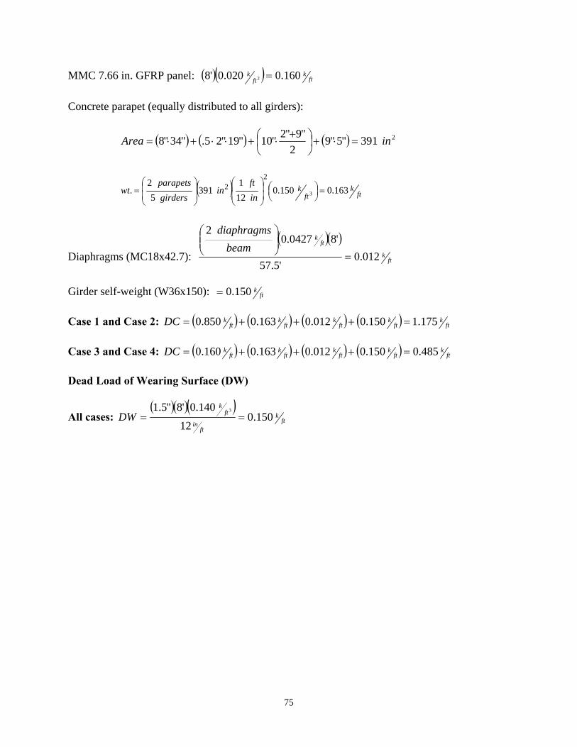
MMC 7.66 in. GFRP panel: ( )( ) ftk

ftk 160.0020.0'8 2 =

Concrete parapet (equally distributed to all girders):

( ) ( ) ( ) 2391"5"92

"9"2"10"19"25."34"8 inArea =⋅+⎟⎠⎞

⎜⎝⎛ +

⋅+⋅⋅+⋅=

( ) ftk

ftk

inft

ingirdersparapets

wt 163.0150.0121

3915

2. 3

22 =⎟

⎠⎞⎜

⎝⎛

⎟⎟⎠

⎞⎜⎜⎝

⎛⎟⎟⎠

⎞⎜⎜⎝

⎛=

Diaphragms (MC18x42.7): ( )( )

ftk

ftk

beamdiaphragms

012.0'5.57

'80427.02

=⎟⎟⎠

⎞⎜⎜⎝

⎛

Girder self-weight (W36x150): ft

k150.0= Case 1 and Case 2: ( ) ( ) ( ) ( ) ft

kft

kft

kft

kft

kDC 175.1150.0012.0163.0850.0 =+++= Case 3 and Case 4: ( ) ( ) ( ) ( ) ft

kft

kft

kft

kft

kDC 485.0150.0012.0163.0160.0 =+++= Dead Load of Wearing Surface (DW)

All cases: ( )( )( )

ftk

ftin

ftk

DW 150.012

140.0'8"5.1 3

==

75

Live Loads (LL)

H20 Loading: (AASHTO 2004)

ftxxxM x 8.2032)14(8 =→=+−⋅−=Σ

14'

8 kips 32 kips

x

R

therefore, for maximum moment position H20 rear axle @ x/2 = 1.4’ to the right of midspan.

1'-434"

28'-9"

-19.03

14'

M(kip-ft)

x338.7

V(kips)

x

20.97

8 kips

x

x

520.5

28'-9"

12.97

32 kips

1'-434"

R

Max H20 LL Moment = 520.5 kip-ft Max H25 LL Moment = 1.25 x 520.5 = 650.6 kip-ft

76

Dead Load Moments: Cases 1 and 2:

Max DC Moment: ( )( ) ftkipwlM DC ⋅=== 6.4858

5.57175.18

22

Max DW Moment: ( )( ) ftkipwlM DW ⋅=== 0.628

5.57150.08

22

Cases 3 and 4:

Max DC Moment: ( )( ) ftkipwlM DC ⋅=== 4.2008

5.57485.08

22

Max DW Moment: ( )( ) ftkipwlM DW ⋅=== 0.628

5.57150.08

22

As per AASHTO LRFD 2004, the Moment Distribution Factor (DF) for Normal Distribution is: Cases 1 and 2:

688.0=DF see Equation 1.3 Therefore the unfactored H25 LL moment for each girder is:

( ) ftkipMftkipM LLLL ⋅=→⋅⋅= 6.4476.650688.0 Cases 3 and 4:

875.0=DF lever rule Therefore the unfactored H25 LL moment for each girder is:

( ) ftkipMftkipM LLLL ⋅=→⋅⋅= 3.5696.650875.0 The STRENGTH I factored moment is: (AASHTO 2004)

( ) DWDCLLU MMMM ⋅+⋅+⋅⋅= 5.125.133.175.1 Cases 1 and 2:

( ) ( ) ( )ftkipftkipftkipMU ⋅⋅+⋅⋅+⋅⋅⋅= 0.625.16.48525.16.44733.175.1 → ftkipMU ⋅= 8.1741

77

Case 3 and Case 4:

( ) ( ) ( )ftkipftkipftkipMU ⋅⋅+⋅⋅+⋅⋅⋅= 0.625.14.20025.13.56933.175.1 → ftkipMU ⋅= 5.1668 The SERVICE I factored moment is: (AASHTO 2004)

( ) DWDCLLU MMMM ⋅+⋅+⋅⋅= 00.100.133.100.1 Cases 1 and 2:

( ) ( ) ( )ftkipftkipftkipMU ⋅⋅+⋅⋅+⋅⋅⋅= 0.6200.16.48500.16.44733.100.1 → ftkipMU ⋅= 9.1142 Case 3 and Case 4:

( ) ( ) ( )ftkipftkipftkipMU ⋅⋅+⋅⋅+⋅⋅⋅= 0.6200.14.20000.13.56933.100.1 → ftkipMU ⋅= 6.1019 The FATIGUE factored moment range is: (AASHTO 2004)

( )LLU MM ⋅⋅= 15.175.0 Cases 1 and 2:

( )ftkipMU ⋅⋅⋅= 6.44715.175.0 → ftkipMU ⋅= 1.386 Cases 3 and 4:

( )ftkipMU ⋅⋅⋅= 3.56915.175.0 → ftkipMU ⋅= 0.491

78

BIBLIOGRAPHY AASHTO, 2004. AASHTO LRFD Bridge Design Specifications, 3rd Edition, American Association of State Highway and Transportation Officials, Washington, D.C. AASHTO, 1996. Standard Specifications for Highway Bridges 16th edition. American Association of State Highway and Transportation Officials, Washington DC. American Composites Manufacturers Association (ACMA) 2004. Global FRP Use for Bridge Applications: Vehicular Bridges. http://www.mdacomposites.org/mda/Bridge_Report_VEH.htm American Institute of Steel Construction (AISC) 2002. Manual of Steel Construction, Load and Resistance Factor Design, 3rd Ed. American Institute of Steel Construction, Chicago. BDI, 2003. Load Testing and Rating Report Update, Fairground Road Bridge, Greene County., Ohio, Bridge Diagnostics Inc., Boulder, Colorado. Black, S. 2003. How are Composite Bridges Performing? Composites Technology, December 2003, pp 16-22. Chandrashekhara, K. and Nanni, A. 2000. Experimental Testing and Modeling of a GFRP Bridge. Report of the Missouri Department of Transportation, Research, Development and Technology Report No. RI 98-032. Crocker, H., Shehata, E., Haldane-Wilson, R. and Mufti A. 2002. Innovative Fibre Reinforced Bridge Deck Modules. Proceedings of the 3rd International Conference on Composites in Infrastructure, San Francisco, CA. Paper # 76. Drexler, A. 2005. Broadway Bridge Deck Panel Testing Report. Portland State University, Portland Oregon. Eom, J. and Nowak, A. 2001. Live Load Distribution for Steel Girder Bridges. ASCE Journal of Bridge Engineering, Vol. 6, No. 6, pp 489-497. Federal Highway Administration (FHWA) 2004. Deficient Bridges by State and Highway System, US Department of Transportation. Federal Highway Administration (FHWA) 2003. Fracture Critical Inspection Techniques for Steel Bridges, US Department of Transportation.

79

GangaRao, H., Thippeswamy, H. K., Shekar, V. and Craigo, C. 1999. “Development of Glass Fiber Reinforced Polymer Composite Bridge Deck.” SAMPE Journal, Vol. 35, No. 4, pp. 12-15. Hooks, J., and O’Connor, J., 2004. A Summary of Six Years Experience Using GFRP Composites for Bridge Decks, Proceedings of the 21st International Bridge Conference, June 12-14, 2004, Pittsburgh, PA. Keelor, D.C., Luo, V., Earls, C.J., and Yulismana, W. 2004. Service Load Effective Compression Flange Width in GFRP Deck Systems Acting Compositely with Steel Stringers, ASCE Journal of Composites for Construction, Vol. 8, No. 4, pp. 289-197. Keller, T and Gurtler, H. 2005. Composite Action and Adhesive Bond Between Fiber-Reinforced Polymer Bridge Decks and Main Girders, ASCE Journal of Composites for Construction, Vol. 9, No. 4, pp. 360-368. Keller, T., Gurtler, H. and Zhou, A. 2004. Performance of Adhesively Bonded GFRP Deck and Steel Bridge Girders, Proceedings of the Fourth Conference on Advanced Composite Materials in Bridges and Structures, Calgary, Canada, July 2004. Paper Number 076. Luo, Y. 2003. The Composite Response Assessment of the Steel Beam-FRP Deck System in the Boyer Bridge, MS Thesis, University of Pittsburgh, Pittsburgh, Pennsylvania. Martin Marietta Composites (MMC) 2001. Duraspan Fiber-reinforced Polymer (FRP) Bridge Deck Technical Literature. Moon, F.L., Eckel, D.A. and Gillespie, J.W., 2002. Shear Stud Connection for the Development of Composite Action Between Steel Girders and Fiber-Reinforced Polymer Bridge Decks, ASCE Journal of Structural Engineering, Vol. 128, No. 6, pp 762-770. Moses, J., Harries, K., Earls, C., and Yulismana, W. 2005. Evaluation of Effective Width and Distribution Factors for GFRP Bridge Decks Supported on Steel Girders, ASCE Journal of Bridge Engineering. (in press). Motley, D. R., Castanos, S. A., Klang, E. C. and Richards, D. 2002. Effects of Diagonal Webs in GFRP Bridge Decks. Proceedings of the 3rd International Conference on Composites in Infrastructure, San Francisco, CA. Paper # 34. National Bridge Inventory (NBI), 2003. http://www.nationalbridgeinventory.com, accessed March 14, 2005. Turner, K.M., 2003. In situ Evaluation of Demonstration GFRP Bridge Deck System Installed on South Carolina Route S655. M.S. Thesis, Department of Civil and Environmental Engineering, University of South Carolina. August 2003. 202 pp. Turner, K.M., Harries, K.A. Petrou, M.F. and Rizos, D. 2004. In-situ Structural Evaluation of GFRP Bridge Deck System. Journal of Composite Structures, Vol. 65 No. 2 pp. 157-165.

80

Turner, K., Harries, K.A. and Petrou, M.F. 2003. In-situ Structural Evaluation of GFRP Bridge Deck System. Proceedings of the 82nd Annual Meeting of the Transportation Research Board, Washington DC, January 2003. Yulismana, W., 2005. Experimental Study of the Behavior of Fiber Reinforced Polymer Bridge Deck System, Ph.D. Dissertation, University of Pittsburgh, Pittsburgh, Pennsylvania. Zhou, A., Lesko, J. J., Coleman, J. T. and Cousins T. E. 2002. Failure Modes and Failure Mechanisms of Fiber Reinforced Polymer Composite Bridge Decks. Proceedings of the 3rd International Conference on Composites in Infrastructure, San Francisco, CA. Paper # 63. Zokaie, T., Imbsen, R, Osterkamp, T., and Wong, T. (1992) Distribution of Wheel Loads on Highway Bridges, NCHRP Project 12-26, National Cooperative Highway Research Program, Washington, D.C.

81