evaluation of climate models using palaeoclimatic data

NATURE OLOGY | ADVANCE ONLINE PUBLICATION | www.nature.com/natureology 1

The fifth phase of the Coupled Model Intercomparison Project (CMIP5) is at present running simulations using state-of-the-art models to provide information about the likely evolution

of climate over the twenty-first century, with additional experiments to analyse the uncertainties inherent in these projections1. Models that perform equally well for present-day climate produce very dif-ferent responses to anthropogenic forcing2,3. Palaeoclimate simula-tions of the Last Glacial Maximum, the mid-Holocene and the Last Millennium are to be included for the first time in the suite of CMIP5 simulations4. Simulations of times in the past when the change in natural forcing was of a similar magnitude to that projected for the next century — and for which abundant palaeoenvironmental data are available for evaluation — provide a unique opportunity to assess model performance outside the climate range for which current models have been developed and, in particular, beyond the calibration range for parameterization that models still necessarily incorporate5,6. The inclusion of the Last Glacial Maximum (LGM; around 21,000 years (21 kyr) ago) and mid-Holocene (around 6 kyr ago) simulations in the CMIP5 experimental design is a reflec-tion of these periods having been major foci for the Palaeoclimate Modelling Intercomparison Project (PMIP; Box 1). This is because both the LGM and the mid-Holocene represent radically different climate states from the present-day and from each other, and have large natural forcings that are relatively well known (Supplementary Table S1). These simulations provide an opportunity to quantify the feedbacks associated with, for example, low carbon dioxide levels, large ice sheets (at the LGM) or vegetation changes (in both the mid-Holocene and LGM).

Evaluation of model simulations against palaeodata shows that models can reproduce the observed direction and large-scale pat-terns of changes in climate at the LGM and mid-Holocene. This would not be possible unless the models incorporated both the

Evaluation of climate models using palaeoclimatic dataPascale Braconnot1, Sandy P. Harrison2, Masa Kageyama1, Patrick J. Bartlein3, Valerie Masson-Delmotte1, Ayako Abe-Ouchi4, Bette Otto-Bliesner5 and Yan Zhao2

There is large uncertainty about the magnitude of warming and how rainfall patterns will change in response to any given scenario of future changes in atmospheric composition and land use. The models used for future climate projections were developed and calibrated using climate observations from the past 40 years. The geologic record of environmental responses to climate changes provides a unique opportunity to test model performance outside this limited climate range. Evaluation of model simulations against palaeodata shows that models reproduce the direction and large-scale patterns of past changes in climate, but tend to underestimate the magnitude of regional changes. As part of the effort to reduce model-related uncertainty and produce more reliable estimates of twenty-first century climate, the Palaeoclimate Modelling Intercomparison Project is systematically applying palaeoevaluation techniques to simulations of the past run with the models used to make future pro-jections. This evaluation will provide assessments of model performance, including whether a model is sufficiently sensitive to changes in atmospheric composition, as well as providing estimates of the strength of biosphere and other feedbacks that could amplify the model response to these changes and modify the characteristics of climate variability.

physics of, and the couplings between, different components of the climate system (land surface, ocean and atmosphere) necessary to simulate climate changes correctly. Thus PMIP climate-model evaluations unequivocally confirm the soundness of the strategy of using global climate models to simulate climates different from the present day. Nevertheless, the simulated magnitude of regional changes is often not as large as the observed magnitude. This may be because models are not sufficiently sensitive to external per-turbations or because they underestimate internal variability6, or it could be caused by incorrect representation of (or failure to include) important feedbacks. Quantifying the difference between observed palaeoclimates and the climate simulated by exactly the same models that are being used for projection of twenty-first cen-tury climate, and isolating the reasons for discrepancies, will be the major task in PMIP3.

Assessing model performance using palaeodata synthesesIce-core, marine and terrestrial archives provide information about environmental responses to past climate changes. These records can be used to derive estimates of climate parameters (that is, they provide proxies for climate) and hence they are sometimes referred to as palaeo-proxies, but here we use the term ‘environmental sen-sors’ because they provide a wider range of information than sim-ply climate. The records can be interpreted to provide qualitative inferences about climate7 or analysed statistically to provide climate reconstructions8. Statistical reconstructions are useful because they allow quantitative comparisons with model simulations, but they generally rely on the assumption that present-day relationships between, for example, pollen assemblages or marine microorgan-isms and climate variables hold in the past (that is, that the sta-tistical relationships are the same and can be mildly extrapolated beyond the calibration range). However, all environmental sensors

1Insitut Pierre Simon Laplace/Laboratoire des Sciences du Climat et de l’Environnement, unité mixte de recherches CEA-CNRS-UVSQ, Orme des Merisiers, bât 712, 91191 Gif sur Yvette Cedex, France, 2School of Biological Sciences, Macquarie University, North Ryde, New South Wales 2109, Australia, 3Department of Geography, University of Oregon, Eugene, Oregon 97403-1251, USA, 4Center for Climate System Research, University of Tokyo, 5-1-5 Kashiwanoha, Kashiwa 277-8569, Japan, 5Climate and Global Dynamics Division, National Center for Atmospheric Research, Boulder, Colorado 80305, USA. *e-mail: [email protected]

REVIEW ARTICLEPUBLISHED ONLINE: 18 MARCH 2012 | DOI: 10.1038/NCLIMATE1456

© 2012 Macmillan Publishers Limited. All rights reserved

mailto:[email protected]

http://www.nature.com/doifinder/10.1038/nclimate1456

2 NATURE CLIMATE CHANGE | ADVANCE ONLINE PUBLICATION | www.nature.com/natureclimatechange

are influenced by non-climatic factors. Atmospheric carbon dioxide concentration directly affects plant growth and competition, and low carbon dioxide levels at the LGM produced changes in terres-trial vegetation patterns (reflected in pollen records) that were as large as those produced by temperature and precipitation changes9. Similarly, changes in ocean circulation affect salinity and mixing depth, and the impact of these changes on marine microorganisms is difficult to separate from the impact of changes in sea surface temperature10. Assessments of the uncertainties inherent in pal-aeoclimate reconstructions are carried out by comparing estimates made using different types of evidence or different reconstruction techniques8,11. These uncertainties, and the much smaller uncer-tainties associated with measurement accuracy, can then be taken into account using statistical techniques that explicitly allow for uncertainties in both observed and simulated climates (for example, refs 12,13). An alternative way of exploiting palaeoenvironmental data for climate-model evaluation is to use models that explicitly simulate the sensor — for example, vegetation14, tree-ring forma-tion15, fire16, peat growth17, glacier mass balance18, marine biogeo-chemistry19, ocean tracers20, the dust cycle21 and stable isotopes of water22 — either in ‘forward’ mode driven by outputs from a climate model15,23–25 or in ‘inverse’ mode to reconstruct more traditional cli-mate variables so that they are consistent with observations26.

PMIP has fostered the production of homogeneous datasets that can serve as benchmarks for model evaluation. There are sev-eral global palaeodata sets available for model evaluation for the mid-Holocene and LGM periods (Supplementary Information), including compilations of existing reconstructions of sea surface temperatures27,28 and bioclimatic variables over land8. To comple-ment the information on environmental parameters, atmospheric composition and temperature from ice cores29–32, PMIP has also focused on assembling spatially explicit datasets that address key aspects of the carbon cycle (Supplementary Information), including peatland dynamics33, fire activity34, dust deposition35 and ocean pro-ductivity36. These datasets allow systematic evaluation (benchmark-ing) of both climate-model simulations (through the use of forward modelling) and the coupled climate–carbon cycle models that are being used for future climate projections1.

What we have learnt from PMIP2Isolating how a change in external conditions (climate forcing) produces a climate response is most tractable in a single, well-known modelling system. The PMIP approach does not preclude such diagnoses, but emphasises the use of multi-model ensembles to identify whether all models show a similar response, or diagnose

the range of possible responses, to a given change in forcing. The assumption is that robust responses that reproduce observed pat-terns of climate change are produced through realistic mechanisms whereas differences in the sign and/or magnitude of response are diagnostic of incorrect or inadequate treatment of the climate processes involved.

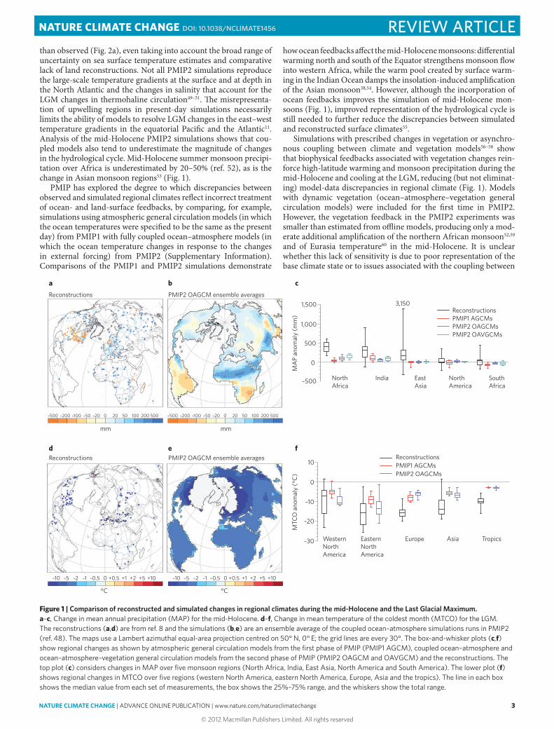
Evaluation of the PMIP2 simulations against palaeodata has clearly established that climate models reproduce the gener-ally colder, drier conditions of the LGM, as well as the large-scale changes in atmospheric circulation caused by the influence of ice sheets on topography37. Similarly, models reproduce the significant enhancement of the Northern Hemisphere monsoons and high-latitude warming during the mid-Holocene38,39. The PMIP2 simula-tions demonstrate that coupled climate models correctly represent large-scale climate features that differ from those at present. This qualitative agreement is illustrated in the comparison between reconstructions and the ensemble-mean of mid-Holocene and LGM model simulations from PMIP2 shown in Fig. 1.

A prominent feature of the palaeorecord, in both cold28,40 and warm41,42 intervals, is the muted surface temperature response of the tropics to changes in forcing compared with the amplification of the temperature response at high latitudes. This feature is present in future projections43. The PMIP2 simulations show polar amplifica-tion (Fig. 2) — although Antarctic cooling is underestimated in the LGM simulations44 — indicating that coupled models are capable of reproducing this signal. Polar amplification is primarily a result of the structure of the polar atmosphere and feedbacks in atmospheric lapse rate, water vapour and clouds that are amplified by changes in sea ice, snow cover and vegetation. Palaeodata also show larger changes in temperature over land than over the ocean in both cold and warm climate intervals (Fig. 2). This ‘land/sea warming ratio’ results from differences in evaporation between land and ocean, and from land-surface feedbacks45. The range for this ratio in pal-aeoclimate simulations46 is similar to that found in future climate projections (1.36–1.84; ref. 47). However, comparisons of simulated and reconstructed LGM temperatures show that values at the higher end of this range are unrealistic (Fig. 2), and thus future simulations showing the most marked contrasts between land and ocean warm-ing probably overestimate the feedback strength.

The PMIP2 simulations are less satisfactory at the regional scale, where they tend to underestimate the magnitude of the observed changes11,24,48,49. Although models simulate the magnitude of LGM cooling over North America (Fig. 1), they underestimate the annual mean cooling of the North Atlantic and Eurasia by at least 3–5 °C (Fig. 2a). Simulated temperatures in the tropics are slightly cooler

The PMIP48,96 emerged from two parallel endeavours. During the 1980s, the Cooperative Holocene Mapping Project97 showed the utility of combining model simulations and syntheses of palaeo-environmental data to analyse the mechanisms of climate change. At the same time, the climate-modelling community was becom-ing increasingly aware that responses to changes in forcing were model dependent. The need to investigate this phenomenon led to the establishment of the Atmospheric Modelling Intercomparison Project (AMIP)98 — the first of a plethora of model intercomparison projects of which PMIP (and CMIP1) are part. The specific aim of PMIP was, and continues to be, to provide a mechanism for coordi-nating palaeoclimate modelling and model-evaluation activities to understand the mechanisms of climate change and the role of cli-mate feedbacks. To facilitate model evaluation, PMIP has actively fostered palaeodata synthesis and the develop ment of benchmark datasets for model evaluation. During its initial phase (PMIP1), the

project focused on atmosphere-only general circulation models; comparisons of coupled ocean–atmosphere and ocean–atmos-phere–vegetation models were the focus of PMIP2 (ref. 48). In PMIP3, project members are running the CMIP5 palaeoclimate simulations and will lead the evaluation of these simulations. However, PMIP3 will also run experiments for non-CMIP5 time periods and will be coordinating the analysis and exploitation of transient simulations across intervals of rapid climate change in the past. PMIP also provides an umbrella for model intercomparison projects focusing on specific times in the past, such as the Pliocene Modelling Intercomparison Project (PLIOMIP)99, or on particular aspects of the palaeoclimate system, such as the Palaeo Carbon Modelling Intercomparison Project (PCMIP)100. PMIP membership is open to all palaeoclimatologists, and we actively encourage the use of archived simulations and data products for model diagnosis or to investigate the causes and impacts of past climate changes.

Box 1 | The Palaeoclimate Modelling Intercomparison Project.

REVIEW ARTICLE NATURE CLIMATE CHANGE DOI: 10.1038/NCLIMATE1456



NATURE CLIMATE CHANGE | ADVANCE ONLINE PUBLICATION | www.nature.com/natureclimatechange 3

than observed (Fig. 2a), even taking into account the broad range of uncertainty on sea surface temperature estimates and comparative lack of land reconstructions. Not all PMIP2 simulations reproduce the large-scale temperature gradients at the surface and at depth in the North Atlantic and the changes in salinity that account for the LGM changes in thermohaline circulation49–51. The misrepresenta-tion of upwelling regions in present-day simulations necessarily limits the ability of models to resolve LGM changes in the east–west temperature gradients in the equatorial Pacific and the Atlantic11. Analysis of the mid-Holocene PMIP2 simulations shows that cou-pled models also tend to underestimate the magnitude of changes in the hydrological cycle. Mid-Holocene summer monsoon precipi-tation over Africa is underestimated by 20–50% (ref. 52), as is the change in Asian monsoon regions53 (Fig. 1).

PMIP has explored the degree to which discrepancies between observed and simulated regional climates reflect incorrect treatment of ocean- and land-surface feedbacks, by comparing, for example, simulations using atmospheric general circulation models (in which the ocean temperatures were specified to be the same as the present day) from PMIP1 with fully coupled ocean–atmosphere models (in which the ocean temperature changes in response to the changes in external forcing) from PMIP2 (Supplementary Information). Comparisons of the PMIP1 and PMIP2 simulations demonstrate

how ocean feedbacks affect the mid-Holocene monsoons: differential warming north and south of the Equator strengthens monsoon flow into western Africa, while the warm pool created by surface warm-ing in the Indian Ocean damps the insolation-induced amplification of the Asian monsoon38,54. However, although the incorporation of ocean feedbacks improves the simulation of mid-Holocene mon-soons (Fig. 1), improved representation of the hydrological cycle is still needed to further reduce the discrepancies between simulated and reconstructed surface climates55.

Simulations with prescribed changes in vegetation or asynchro-nous coupling between climate and vegetation models56–58 show that biophysical feedbacks associated with vegetation changes rein-force high-latitude warming and monsoon precipitation during the mid-Holocene and cooling at the LGM, reducing (but not eliminat-ing) model-data discrepancies in regional climate (Fig. 1). Models with dynamic vegetation (ocean–atmosphere–vegetation general circulation models) were included for the first time in PMIP2. However, the vegetation feedback in the PMIP2 experiments was smaller than estimated from offline models, producing only a mod-erate additional amplification of the northern African monsoon52,59 and of Eurasia temperature60 in the mid-Holocene. It is unclear whether this lack of sensitivity is due to poor representation of the base climate state or to issues associated with the coupling between

Reconstructions PMIP2 OAGCM ensemble averages

Reconstructions PMIP2 OAGCM ensemble averages

–500 –100–200 –50 –20 50020010050200 –500 –100–200 –50 –20 50020010050200

1,500

1,000

500

0

–500

MA

P an

omal

y (m

m)

a b

d e

c

f

mm mm

–10 +10–5 +5–2 +2–1 +1–0.5 +0.50

°C

–10 +10–5 +5–2 +2–1 +1–0.5 +0.50

°C

10

0

–10

–20

–30

MTC

O a

nom

aly

(°C

)

NorthAfrica

India EastAsia

NorthAmerica

SouthAfrica

WesternNorthAmerica

EasternNorthAmerica

Europe Asia Tropics

ReconstructionsPMIP1 AGCMsPMIP2 OAGCMs

ReconstructionsPMIP1 AGCMsPMIP2 OAGCMsPMIP2 OAVGCMs

3,150

Figure 1 | Comparison of reconstructed and simulated changes in regional climates during the mid-Holocene and the Last Glacial Maximum. a–c, Change in mean annual precipitation (MAP) for the mid-Holocene. d–f, Change in mean temperature of the coldest month (MTCO) for the LGM. The reconstructions (a,d) are from ref. 8 and the simulations (b,e) are an ensemble average of the coupled ocean–atmosphere simulations runs in PMIP2 (ref. 48). The maps use a Lambert azimuthal equal-area projection centred on 50° N, 0° E; the grid lines are every 30°. The box-and-whisker plots (c,f) show regional changes as shown by atmospheric general circulation models from the first phase of PMIP (PMIP1 AGCM), coupled ocean–atmosphere and ocean–atmosphere–vegetation general circulation models from the second phase of PMIP (PMIP2 OAGCM and OAVGCM) and the reconstructions. The top plot (c) considers changes in MAP over five monsoon regions (North Africa, India, East Asia, North America and South America). The lower plot (f) shows regional changes in MTCO over five regions (western North America, eastern North America, Europe, Asia and the tropics). The line in each box shows the median value from each set of measurements, the box shows the 25%–75% range, and the whiskers show the total range.

REVIEW ARTICLENATURE CLIMATE CHANGE DOI: 10.1038/NCLIMATE1456




vegetation, soil moisture and land-surface exchanges61. In view of the failure of current models to reproduce the magnitude and regional patterns of past changes in the monsoon, this apparent lack of sensitivity to vegetation feedbacks raises concerns about the credibility of land-surface representation in ocean–atmosphere–vegetation general circulation models, and our ability to assess the impact of natural and anthropogenic land-cover changes on future climates62.

A further focus in PMIP has been on how external forcing and the mean climate state affects interannual variability, and how this is linked, in particular, to changes in the ocean and changes in modes of atmospheric circulation (for example, the North Atlantic Oscillation and El Niño/Southern Oscillation (ENSO)). PMIP2 mid-Holocene simulations show little change relative to present in the North Atlantic Oscillation63, but show reduced ENSO vari-ability64 that is apparently consistent with coral-based reconstruc-tions65. However, sensitivity experiments suggest that the impact of changing seasonality on sea surface temperatures is as impor-tant as changes in interannual variability66; further analyses of the coral records will be required to disentangle the two mechanisms. The mid-Holocene simulations also show changes in the strength of teleconnections with ENSO67, including the teleconnection with Sahel precipitation68. Changes in short-term variability and in the persistence of extremes can have as large an impact on vegetation cover as a shift in mean climate69, and thus changes in variabil-ity may be crucial to understanding land-surface feedbacks at a regional scale. One important result emerging from the analyses of records of interannual to multidecadal variability is that the spa-tial ‘fingerprint’ of atmospheric circulation modes varies through time without large external forcing70,71. There is little consistency about how atmospheric circulation modes will change in the future72, and therefore it is important to continue exploring the role of forced and unforced responses (and potential feedbacks) in the past.

Uncertainties in forcing and boundary conditions Models translate changes in the variables influencing climate on a specific timescale (‘boundary conditions’; Supplementary Table S1) into a radiative perturbation, which in turn is translated into changes in the global heat budget and hydrological cycle. However, as shown by future projections and palaeoexperiments43,52,73, dif-ferent models show different sensitivity to an initial perturbation. Climate sensitivity is conventionally defined as the change in global temperature in response to a doubling of carbon dioxide concentra-tion, but the concept applies equally well to other changes in climate forcing. Correctly simulating the way in which a given change in forcing propagates through the climate system and is affected by internal feedbacks is central to the prediction of future climate74. Palaeosimulations provide an opportunity to evaluate whether internal feedbacks are correctly simulated, providing it is possible to identify the impact of structural differences (or model biases) on effective radiative forcing37,75 and to quantify uncertainties in boundary conditions.

Boundary conditions — including insolation, atmospheric trace-gas concentration, land–sea geography and orography, land-surface surface type and river pathways — are specified for the CMIP5 pal-aeoclimate experiments (Supplementary Table S1). However, even though each model uses the same changes in boundary conditions, differences in model construction lead to differences in the effec-tive radiative perturbation computed in each model (Fig. 3 and Supplementary Table S2). For example, the mean modern surface albedo of regions covered by the LGM ice sheets ranges from 0.26 to 0.36 in the PMIP2 simulations. This spread results mainly from the representation of snow cover in the modern climate: models with a higher modern albedo produce a global shortwave ice-sheet and land albedo forcing in the lower part of the range of PMIP2 estimates (–3.48 to –2.59 W m–2; Fig. 3). In this estimate, the ice-sheet forcing ranges from –1.8 to –2.3 W m–2 and the albedo forcing from land exposed by the lower sea level at the LGM ranges from

–10 –5 0 –10 –5 0

0

–5

–10

0

–5

–10

Oce

an te

mpe

ratu

re c

hang

e (°

C)

Regi

onal

tem

pera

ture

cha

nge

(°C

)

Tropics – PMIP2 OAGCM

Tropics – reconstructions

North Atlantic Europe – PMIP2 OAGCMNorth Atlantic Europe – reconstructions

Tropical oceans – PMIP2 OAGCMEast Antarctica – PMIP2 OAGCM

a b

Land temperature change (°C) Global temperature change (°C)

Figure 2 | Relationships between key temperature indices at the Last Glacial Maximum as shown by observations and model simulations. a, The relationship between changes in mean annual temperature over ocean and land in the tropics (red) and changes in mean annual temperature over the North Atlantic and in Europe (blue). The squares show the mean value of the reconstructions, with the range shown in black. The diamonds are the results of individual coupled ocean–atmosphere general circulation models from the second phase of PMIP (PMIP2 OAGCM), where the bars show the range of simulated values from that model. The diagonal line shows the 1:1.5 ratio between ocean and land temperature anomalies, for illustration (see text). b, The simulated relationship between global cooling and regional cooling of the tropical oceans and over East Antarctica. The shaded panels show the range of reconstructed mean annual temperatures in the tropics (red) and over East Antarctica (blue); the red circles show tropical temperatures as simulated by individual coupled ocean–atmosphere general circulation models from the second phase of PMIP (PMIP2 OAGCM) and the blue crosses show simulated temperatures over East Antarctica from the same simulations.





–0.7 to –1.3 W m–2. The higher elevation of the ice sheet at the LGM also leads to colder surface temperatures and thereby alters the longwave emission to space by about –3.2 to –3.5 W m–2. The effect of the prescribed ice-sheet elevation has not been quantified as a forcing previously, but is critical for understanding regional changes over Antarctica44. These differences between models explain part of the range (–3 to –6 °C) in the simulated global LGM cooling. The remainder can be attributed to differences in climate feedbacks aris-ing from changes in surface albedo (due to changes in, for example, vegetation, ice or snow cover), atmospheric scattering and clouds, factors contributing to changes in longwave radiation (such as atmospheric lapse rates, water vapour and cloud feedbacks), and ocean heat uptake. Cloud feedbacks account for a large part of the model scatter in these feedbacks (Fig. 3)

Insolation and atmospheric composition at the LGM are known, but some other forcings are less well constrained. PMIP experi-ments have shown that there is considerable sensitivity to ice-sheet topography44. There are several possible configurations of LGM ice sheets (extent, orography) that are consistent with relative sea-level and geoidal constraints76–78. The LGM ice sheets created for CMIP5 are a blended product made from three of the latest ice-sheet recon-structions (https://pmip3.lsce.ipsl.fr/wiki/doku.php/pmip3:design:pi:final:icesheet), but each ice-sheet reconstruction will also be used in PMIP3 to test the sensitivity of the model results to the uncer-tainties in the ice-sheet specification. Estimates made using PMIP2 data suggest that the difference in the land–sea mask between the PMIP2 and PMIP3 experiments will lead to an additional forcing of around 0.6 W m–2, and the difference in ice-sheet elevation will lead to about 0.6 °C warmer conditions in the PMIP3 simulations, equivalent to a 1–3 W m–2 difference in the longwave-radiation forc-ing due to orography.

In the mid-Holocene experiment, the change in Earth’s orbital parameters (Supplementary Table S1) induces virtually no change in annual mean insolation but leads to a 30 to 60 W m–2 change in seasonal insolation shortwave forcing at the top of the atmosphere. In this case, the effective forcing can be estimated as net change in solar radiation at the top of the atmosphere, with the assumption that the planetary albedo is the same as at present48. Regional biases in the simulation of the pre-industrial planetary albedo (linked to the representation of convection, clouds, and snow and ice surfaces

in the models) thus have a major impact on the effective forcing, and may trigger erroneous feedbacks.

What we hope to learn in PMIP3Although not specifically designed as adjuncts to the projec-tion of future climate changes, evaluation of PMIP climate-model simulations against palaeodata are critical tests of whether climate models can reproduce the amplitude, timing and nonlinear feed-backs involved in climate change at the global and regional scale. Palaeoevaluation of the models being used for future projections in CMIP5, however, provides new opportunities to address issues that are critical for improved understanding of the trajectory of twenty-first century climate.

One area in which we expect to make substantial progress is in providing a well-founded constraint on climate sensitivity — the global temperature response to a doubling of carbon dioxide con-centration. Previous attempts to do this using palaeodata and mod-elling have focused on the LGM79,80, chiefly because the simulated global cooling at the LGM is of a similar magnitude to the warming expected at the end of next century. The response is not independent of climate state and climate forcing, mainly because of differences in cloud feedback79,81. This has motivated the inclusion of past warm intervals in PMIP3 to study climate sensitivity in climate states that are more comparable to future climates. A continued focus on the LGM is nevertheless justified, because the change in global temper-ature is large and well characterized, and the cooling of the tropics and Antarctica at the LGM is primarily a response to lower carbon dioxide levels52,82. The goal is not to estimate climate sensitivity at the LGM directly, but rather to establish which model best repro-duces observed LGM climates, on the assumption that this model is most likely to have a realistic climate sensitivity under modern conditions. A recent study adopting this approach compared results from a single intermediate complexity model ensemble with LGM observed temperature anomalies, and showed that the best esti-mate of the median climate sensitivity for the century timescale was 2.3 °C, with a likely range of 1.4–4.3 °C, which effectively rules out climate sensitivities greater than 6 °C (ref. 83). One task in PMIP3 will be to test this conclusion using a larger range of models because, although the range of sensitivities in these simulations are larger than those obtained from other single-model ensembles (for

Forcing

Longwave radiation (altitude)

Longwave radiation (residual)

FeedbackSurface albedo

Carbon dioxide

Atmosphere (scattering and clouds)

–6 –5 –4 –3 –2 –1 0 1

(W m–2)

LGM forcing (W m–2)–100 –50 –10–20 –5

Total (ice sheet + land)

Figure 3 | Estimation of the difference in radiative forcing and feedbacks at the LGM compared with pre-industrial conditions caused by changes in boundary conditions. The map is a composite of the results from six PMIP2 ocean–atmosphere models showing the spatial patterns of the change in total forcing associated with the expanded Northern Hemisphere ice sheets at the LGM and with the increase of land area due to lowered sea level. The map uses a Robinson projection centred on 0°, 0°; the grid lines are every 30°. Differences in the effective radiative perturbation computed in each model for individual components of the overall forcing are shown on the right-hand side. The change in longwave radiation represents a bulk greenhouse effect estimated from the difference between surface emission and outgoing longwave radiation at the top of the atmosphere. At the LGM, lower atmospheric trace-gas concentrations induce a longwave perturbation of −2.8 W m−2. Model spread is estimated to be 0.4–0.6 W m–2. See Supplementary Information for details of the method.



https://pmip3.lsce.ipsl.fr/wiki/doku.php/pmip3:design:pi:final:icesheet

https://pmip3.lsce.ipsl.fr/wiki/doku.php/pmip3:design:pi:final:icesheet



example, ref. 13), there are some aspects of the simulated regional climates that are not consistent with observations.

Evaluation of climate sensitivity is part of a wider strategy of model benchmarking. PMIP has now assembled independent benchmark datasets that allow multi-parameter evaluation of model skill for the CMIP5 mid-Holocene and LGM experiments (Supplementary Information), and will use these datasets to evaluate model perfor-mance quantitatively at both global and regional scales. Past climates will then provide a complete evaluation of the robustness of the rep-resentation of dynamical, physical and biogeochemical processes included in climate models. The emphasis on regional benchmark-ing is because models that reproduce large-scale features of past cli-mates reasonably well (for example, zonal cooling at the LGM) do not necessarily reproduce the regional patterns of change correctly. Similarly, a model may represent the observed change in one region and fail to capture the correct change in another, and correct simula-tion of surface climate does not guarantee that, for example, carbon-cycle feedbacks will also be correct. The motivation for evaluation is to inform model development, but given the increasingly urgent need to predict and manage the impacts of anthropogenic forcing, palaeobenchmarking should also provide guidance for selecting an appropriate subset of models based on process-oriented studies to be used for regional assessment exercises.

The Last Millennium (850–1850 ad) is included in the CMIP5 suite of palaeosimulations to examine natural climate variability in a climate state close to that of the present day84 and to serve as a reference for detecting and attributing observed twentieth-century changes in climate patterns and trends resulting from anthropo-genic activities85. A preliminary comparison of pre-CMIP5 Last Millennium simulations shows that models have some skill in reproducing the Last Millennium trends. However, inconsistencies between simulations and reconstructions suggest either that the changes between the Medieval Warm Period (950–1250 ad) and the Little Ice Age (1400–1700 ad) arose mainly from internal variabil-ity, or that transient simulations with state-of the-art models fail to reproduce some mechanisms of response to external forcing cor-rectly86. Quantification of uncertainties in climate forcings is thus critical for Last Millennium simulations, and the CMIP5 protocol defines a number of alternative forcing histories to take account of the large uncertainties in solar, volcanic and land-use forcing over this period. The range of these ‘scenarios’ is sufficiently large so that the structural uncertainty in forcing can be appropriately considered in a coherent model framework. The Last Millennium has not been a focus for PMIP until now, but provides opportunities to investi-gate the link between volcanism and ENSO variability87,88, to test the stability (or otherwise) of atmospheric modes, to analyse the inter-action between short-term variability and land-surface feedbacks, and to explore changes in recurrence or intensity of extreme events, including their societal impacts from historical archives89. However, the major task will be quantification of the carbon-cycle feedback, capitalizing on PMIP expertise in the use of multiple palaeoenvi-ronmental datasets for model evaluation and using new syntheses of high-resolution vegetation, peatland and fire data90.

PMIP3 activities are not confined to analyses and evaluation of the three CMIP5 palaeosimulations. There will be simulations of other warm periods, either orbitally driven (the last interglacial, 125 kyr ago) or carbon dioxide-driven (the mid-Pliocene, around 3.3–3.0 Myr ago). Planned simulations of Greenland stadials will test the simulation of cold climates with a different ice-sheet con-figuration and different greenhouse-gas concentrations from the LGM. The additional equilibrium experiments broaden the scope of the PMIP contribution to CMIP5, by offering additional oppor-tunities to test the mechanisms documented in the LGM and mid-Holocene simulations. They also provide a way of quantifying the sensitivity to individual boundary conditions, and, through com-parison with independent palaeodata sets40,41,91–93, of evaluating

whether this sensitivity is realistic. Transient experiments are now possible using the CMIP5 class of models94 and will explore the abrupt and widespread climate changes, most probably associated with freshwater inputs to the North Atlantic, that are characteristic of the last glacial and the last deglaciation40. The transient experi-ments provide opportunities to explore aspects of dynamic behav-iour that will not be expressed in the Last Millennium simulation. Specifically, they provide an opportunity to investigate interactions between ice-sheet and ocean dynamics, and to evaluate the realism of threshold behaviour, including that leading to rapid ice-sheet melting and thereby to sea-level rise95 — which could be important in the future.

PMIP has already done much to elucidate the mechanisms of climate change and to demonstrate the ability of climate models to simulate such changes. Our task in CMIP5 is to make use of the coherent framework between past, present and future simulations to provide a systematic and quantitative assessment of the realism of the models used to predict the future.

References1. Taylor, K. E., Stouffer, R. J. & Meehl, G. A. An overview of CMIP5

and the experiment design. Bull. Am. Meteorol. Soc. http://dx.doi.org/BAMS-D-11-00094.1 (2011).

2. Doherty, S. J. et al. Lessons learned from IPCC AR4: Scientific developments needed to understand, predict, and respond to climate change. Bull. Am. Meteorol. Soc. 90, 497-513 (2009).

3. Knutti, R., Furrer, R., Tebaldi, C., Cermak, J. & Meehl, G. A. Challenges in combining projections from multiple climate models. J. Clim. 23, 2739–2758 (2010).

4. Braconnot, P. et al. The Paleoclimate Modeling Intercomparison Project contribution to CMIP5. CLIVAR Exchanges No. 56 16, 15–19 (2011).

5. Schmidt, G. A. Enhancing the relevance of palaeoclimate model/data comparisons for assessments of future climate change. J. Quat. Sci. 25, 79–87 (2010).

6. Valdes, P. Built for stability. Nature Geosci. 4, 414–416 (2011).7. Kohfeld, K. E. & Harrison, S. P. How well can we simulate past climates?

Evaluating the models using global palaeoenvironmental datasets. Quat. Sci. Rev. 19, 321–346 (2000).

8. Bartlein, P. J. et al. Pollen-based continental climate reconstructions at 6 and 21 ka: A global synthesis. Clim. Dynam. 37, 775–802 (2011).

9. Harrison, S. & Prentice, C. Climate and CO2 controls on global vegetation distribution at the last glacial maximum: Analysis based on palaeovegetation data, biome modelling and palaeoclimate simulations. Glob. Change Biol. 9, 983–1004 (2003).

10. Richey, J. N., Hollander, D. J., Flower, B. P. & Eglinton, T. I. Merging late Holocene molecular organic and foraminiferal-based geochemical records of sea surface temperature in the Gulf of Mexico. Paleoceanography 26, PA1209 (2011).

11. Otto-Bliesner, B. L. et al. A comparison of PMIP2 model simulations and the MARGO proxy reconstruction for tropical sea surface temperatures at last glacial maximum. Clim. Dynam. 32, 799–815 (2009).

12. Brewer, S., Guiot, J. & Torre, F. Mid-Holocene climate change in Europe: A data-model comparison. Clim. Past 3, 499–512 (2007).

13. Hargreaves, J. C., Paul, A., Ohgaito, R., Abe-Ouchi, A. & Annan, J. D. Are paleoclimate model ensembles consistent with the MARGO data synthesis? Clim. Past 7, 917–933 (2011).

14. Kaplan, J. O. et al. Climate change and Arctic ecosystems: 2. Modeling, paleodata-model comparisons, and future projections. J. Geophys. Res. 108, D198171 (2003).

15. Evans, M. N. et al. A forward modeling approach to paleoclimatic interpretation of tree-ring data. J. Geophys. Res. 111, G03008 (2006).

16. Prentice, I. C. et al. Modeling fire and the terrestrial carbon balance. Glob. Biogeochem. Cycles 25, GB3005 (2011).

17. Gallego-Sala, A. V. et al. Bioclimatic envelope model of climate change impacts on blanket peatland distribution in Great Britain. Clim. Res. 45, 151–162 (2010).

18. Michlmayr, G. et al. Application of the Alpine 3D model for glacier mass balance and glacier runoff studies at Goldbergkees, Austria. Hydrol. Process. 22, 3941–3949 (2008).

19. Bopp, L., Kohfeld, K. E., Le Quere, C. & Aumont, O. Dust impact on marine biota and atmospheric CO2 during glacial periods. Paleoceanography 18, 1046 (2003).

20. Huhn, K., Paul, A. & Seyferth, M. Modeling sediment transport patterns during an upwelling event. J. Geophys. Res. 112, C10003 (2007).





21. Werner, M. et al. Seasonal and interannual variability of the mineral dust cycle under present and glacial climate conditions. J. Geophys. Res. 108, 47744 (2003).

22. Sturm, C., Zhang, Q. & Noone, D. An introduction to stable water isotopes in climate models: Benefits of forward proxy modelling for paleoclimatology. Clim. Past 6, 115–129 (2010).

23. Harrison, S. P. et al. Intercomparison of simulated global vegetation distributions in response to 6 kyr bp orbital forcing. J. Clim. 11, 2721–2742 (1998).

24. Coe, M. T. & Harrison, S. P. The water balance of northern Africa during the mid-Holocene: An evaluation of the 6 ka bp PMIP simulations. Clim. Dynam. 19, 155–166 (2002).

25. Bassinot, F. et al. Holocene evolution of summer winds and marine productivity in the tropical Indian Ocean in response to insolation forcing: Data-model comparison. Clim. Past 7, 815–829 (2011).

26. Wu, H. B., Guiot, J. L., Brewer, S. & Guo, Z. T. Climatic changes in Eurasia and Africa at the last glacial maximum and mid-Holocene: Reconstruction from pollen data using inverse vegetation modelling. Clim. Dynam. 29, 211–229 (2007).

27. Kim, J. H. et al. North Pacific and North Atlantic sea-surface temperature variability during the holocene. Quat. Sci. Rev. 23, 2141–2154 (2004).

28. Waelbroeck, C. et al. Constraints on the magnitude and patterns of ocean cooling at the Last Glacial Maximum. Nature Geosci. 2, 127–132 (2009).

29. Jouzel, J. et al. The GRIP deuterium-excess record. Quat. Sci. Rev. 26, 1–17 (2007).

30. Luthi, D. et al. High-resolution carbon dioxide concentration record 650,000–800,000 years before present. Nature 453, 379–382 (2008).

31. Loulergue, L. et al. Orbital and millennial-scale features of atmospheric CH4 over the past 800,000 years. Nature 453, 383–386 (2008).

32. Elsig, J. et al. Stable isotope constraints on Holocene carbon cycle changes from an Antarctic ice core. Nature 461, 507–510 (2009).

33. Yu, Z. C., Loisel, J., Brosseau, D. P., Beilman, D. W. & Hunt, S. J. Global peatland dynamics since the Last Glacial Maximum. Geophys. Res. Lett. 37, L13402 (2010).

34. Power, M. J. et al. Changes in fire regimes since the Last Glacial Maximum: An assessment based on a global synthesis and analysis of charcoal data. Clim. Dynam. 30, 887–907 (2008).

35. Kohfeld, K. E. & Harrison, S. P. DIRTMAP: The geological record of dust. Earth Sci. Rev. 54, 81–114 (2001).

36. Radi, T. & de Vernal, A. Last glacial maximum (LGM) primary productivity in the northern North Atlantic Ocean. Can. J. Earth Sci. 45, 1299–1316 (2008).

37. Jansen, E. et al. in IPCC Climate Change 2007: The Physical Science Basis (eds Solomon, S. et al.) 385–432 (Cambridge Univ. Press, 2007).

38. Zhao, Y. et al. A multi-model analysis of the role of the ocean on the African and Indian monsoon during the mid-Holocene. Clim. Dynam. 25, 777–800 (2005).

39. Wohlfahrt, J. et al. Evaluation of coupled ocean–atmosphere simulations of the mid-Holocene using palaeovegetation data from the Northern Hemisphere extratropics. Clim. Dynam. 31, 871–890 (2008).

40. Harrison, S. P. & Goni, M. F. S. Global patterns of vegetation response to millennial-scale variability and rapid climate change during the last glacial period. Quat. Sci. Rev. 29, 2957–2980 (2010).

41. Anderson, P. et al. Last Interglacial Arctic warmth confirms polar amplification of climate change. Quat. Sci. Rev. 25, 1383–1400 (2006).

42. Miller, G. H. et al. Arctic amplification: Can the past constrain the future? Quat. Sci. Rev. 29, 1779–1790 (2010).

43. Meehl, G. A. et al. in IPCC Climate Change 2007: The Physical Science Basis (eds Solomon, S. et al.) 747–845 (Cambridge Univ. Press, 2007).

44. Masson-Delmotte, V. et al. EPICA Dome C record of glacial and interglacial intensities. Quat. Sci. Rev.29, 113–128 (2010).

45. Joshi, M. M., Gregory, J. M., Webb, M. J., Sexton, D. M. H. & Johns, T. C. Mechanisms for the land/sea warming contrast exhibited by simulations of climate change. Clim. Dynam. 30, 455–465 (2008).

46. Laine, A., Kageyama, M., Braconnot, P. & Alkama, R. Impact of greenhouse gas concentration changes on surface energetics in IPSL-CM4: Regional warming patterns, land–sea warming ratios, and glacial–interglacial differences. J. Clim. 22, 4621–4635 (2009).

47. Sutton, R. T., Dong, B. W. & Gregory, J. M. Land/sea warming ratio in response to climate change: IPCC AR4 model results and comparison with observations. Geophys. Res. Lett. 34, L02701 (2007).

48. Braconnot, P. et al. Results of PMIP2 coupled simulations of the Mid-Holocene and Last Glacial Maximum — Part 1: Experiments and large-scale features. Clim. Past 3, 261–277 (2007).

49. Kageyama, M. et al. Last Glacial Maximum temperatures over the North Atlantic, Europe and western Siberia: A comparison between PMIP models, MARGO sea-surface temperatures and pollen-based reconstructions. Quat. Sci. Rev. 25, 2082–2102 (2006).

50. Otto-Bliesner, B. L. et al. Last Glacial Maximum ocean thermohaline circulation: PMIP2 model intercomparisons and data constraints. Geophys. Res. Lett. 34, L12706 (2007).

51. Weber, S. L. et al. The modern and glacial overturning circulation in the Atlantic Ocean in PMIP coupled model simulations. Clim. Past 3, 51–64 (2007).

52. Braconnot, P. et al. Results of PMIP2 coupled simulations of the Mid-Holocene and Last Glacial Maximum — Part 2: Feedbacks with emphasis on the location of the ITCZ and mid- and high latitudes heat budget. Clim. Past 3, 279–296 (2007).

53. Zhao, Y. & Harrison, S. P. Mid-Holocene monsoons: A multi-model analysis of the inter-hemispheric differences in the responses to orbital forcing and ocean feedbacks. Clim. Dynam. http://dx.doi.org/10.1007/s00382-011-1193-z (2011).

54. Ohgaito, R. & Abe-Ouchi, A. The role of ocean thermodynamics and dynamics in Asian summer monsoon changes during the mid-Holocene. Clim. Dynam. 29, 39–50 (2007).

55. Ohgaito, R. & Abe-Ouchi, A. The effect of sea surface temperature bias in the PMIP2 AOGCMs on mid-Holocene Asian monsoon enhancement. Clim. Dynam. 33, 975–983 (2009).

56. Wohlfahrt, J., Harrison, S. P. & Braconnot, P. Synergistic feedbacks between ocean and vegetation on mid- and high-latitude climates during the mid-Holocene. Clim. Dynam. 22, 223–238 (2004).

57. Jahn, A., Claussen, M., Ganopolski, A. & Brovkin, V. Quantifying the effect of vegetation dynamics on the climate of the Last Glacial Maximum. Clim. Past 1, 1–7 (2005).

58. Braconnot, P., Joussaume, S., Marti, O. & de Noblet, N. Synergistic feedbacks from ocean and vegetation on the African monsoon response to mid-Holocene insolation. Geophys. Res. Lett. 26, 2481–2484 (1999).

59. Levis, S., Bonan, G. B. & Bonfils, C. Soil feedback drives the mid-Holocene North African monsoon northward in fully coupled CCSM2 simulations with a dynamic vegetation model. Clim. Dynam. 23, 791–802 (2004).

60. Otto, J., Raddatz, T., Claussen, M., Brovkin, V. & Gayler, V. Separation of atmosphere–ocean–vegetation feedbacks and synergies for mid-Holocene climate. Glob. Biogeochem. Cycles 23, L09701 (2009).

61. Wang, Y. et al. Detecting vegetation–precipitation feedbacks in mid-Holocene North Africa from two climate models. Clim. Past 4, 59–67 (2008).

62. Pitman, A. J. et al. Importance of background climate in determining impact of land-cover change on regional climate. Nature Clim. Change 1, 472–475 (2011).

63. Gladstone, R. M. et al. Mid-Holocene NAO: A PMIP2 model intercomparison. Geophys. Res. Lett. 32, L16707 (2005).

64. Zheng, W., Braconnot, P., Guilyardi, E., Merkel, U. & Yu, Y. ENSO at 6ka and 21ka from ocean–atmosphere coupled model simulations. Clim. Dynam. 30, 745–762 (2008).

65. Tudhope, A. W. et al. Variability in the El Niño–Southern Oscillation through a glacial–interglacial cycle. Science 291, 1511–1517 (2001).

66. Braconnot, P., Luan, Y., Brewer, S. & Zheng, W. Impact of Earth’s orbit and freshwater fluxes on Holocene climate mean seasonal cycle and ENSO characteristics. Clim. Dynam. 38, 1081–1092 (2012).

67. Harrison, S. P. & Bartlein, P. J. in The Future of the World’s Climates (eds Henderson-Sellers, A. & McGuffie, K.) 403–436 (Elsevier, 2012).

68. Zhao, Y., Braconnot, P., Harrison, S. P., Yiou, P. & Marti, O. Simulated changes in the relationship between tropical ocean temperatures and the western African monsoon during the mid-Holocene. Clim. Dynam. 28, 533–551 (2007).

69. Ni, J., Harrison, S. P., Prentice, I. C., Kutzbach, J. E. & Sitch, S. Impact of climate variability on present and Holocene vegetation: A model-based study. Ecol. Model. 191, 469–486 (2006).

70. Cobb, K. M., Charles, C. D., Cheng, H. & Edwards, R. L. El Niño/Southern Oscillation and tropical Pacific climate during the last millennium. Nature 424, 271–276 (2003).

71. Wittenberg, A. T. Are historical records sufficient to constrain ENSO simulations? Geophys. Res. Lett. 36, L12702 (2009).

72. Guilyardi, E. et al. Understanding El Niño in ocean–atmosphere general circulation models: Progress and challenges. Bull. Am. Meteorol. Soc. 90, 325–340 (2009).

73. Crucifix, M. Does the Last Glacial Maximum constrain climate sensitivity? Geophys. Res. Lett. 33, L18701 (2006).

74. Bony, S. et al. How well do we understand and evaluate climate change feedback processes? J. Clim. 19, 3445–3482 (2006).

75. Hegerl, G. C. et al. in IPCC Climate Change 2007: The Physical Science Basis (eds Solomon, S. et al.) 665–775 (Cambridge Univ. Press, 2007).

76. Lambeck, K., Yokoyama, Y. & Purcell, T. Into and out of the Last Glacial Maximum: Sea-level change during oxygen isotope stages 3 and 2. Quat. Sci. Rev. 21, 343–360 (2002).

77. Tarasov, L. & Peltier, W. R. Greenland glacial history and local geodynamic consequences. Geophys. J. Int. 150, 198–229 (2002).





78. Engelhart, S. E., Peltier, W. R. & Horton, B. P. Holocene relative sea-level changes and glacial isostatic adjustment of the US Atlantic coast. Geology 39, 751–754 (2011).

79. Hargreaves, J. C. & Annan, J. D. Using ensemble prediction methods to examine regional climate variation under global warming scenarios. Ocean Model. 11, 174–192 (2006).

80. Schneider von Deimling, T., Held, H., Ganopolski, A. & Rahmstorf, S. Climate sensitivity estimated from ensemble simulations of glacial climate. Clim. Dynam. 27, 149–163 (2006).

81. Yoshimori, M., Yokohata, T. & Abe-Ouchi, A. A comparison of climate feedback strength between CO2 doubling and LGM experiments. J. Clim. 22, 3374–3395 (2009).

82. Hewitt, C. & Mitchell, J. F. B. Radiative forcing and response of a GCM to ice age boundary conditions: Cloud feedback and climate sensitivity. Clim. Dynam. 13, 821–834 (1997).

83. Schmittner, A. et al. Climate sensitivity estimated from temperature reconstructions of the Last Glacial Maximum. Science 334, 1385–1388 (2011).

84. Schmidt, G. A. et al. Climate forcing reconstructions for use in PMIP simulations of the last millennium (v1.0). Geoscientific Model Dev. 4, 33–45 (2011).

85. Hegerl, G. J. et al. Influence of human and natural forcing on European seasonal temperatures Nature Geosci. 4, 99–103 (2011).

86. González-Rouco, F. J. et al. Medieval Climate Anomaly to Little Ice Age transition as simulated by current climate models. PAGES news 19, 7–11 (2011).

87. Emile-Geay, J., Seager, R., Cane, M. A., Cook, E. R. & Haug, G. H. Volcanoes and ENSO over the past millennium. J. Clim. 21, 3134–3148 (2008).

88. Wilson, R. et al. Reconstructing ENSO: The influence of method, proxy data, climate forcing and teleconnections. J. Quat. Sci. 25, 62–78 (2010).

89. IPCC Special Report on Managing the Risks of Extreme Events and Disasters to Advance Climate Change Adaptation (eds Field, C. B. et al.) (Cambridge Univ. Press, 2011).

90. Marlon, J. R. et al. Climate and human influences on global biomass burning over the past two millennia. Nature Geosci. 1, 697–702 (2008).

91. Salzmann, U., Haywood, A. M., Lunt, D. J., Valdes, P. J. & Hill, D. J. A new global biome reconstruction and data-model comparison for the Middle Pliocene. Glob. Ecol. Biogeogr. 17, 432–447 (2008).

92. Dowsett, H. J., Robinson, M. M. & Foley, K. M. Pliocene three-dimensional global ocean temperature reconstruction. Clim. Past 5, 769–783 (2009).

93. Daniau, A. L., Harrison, S. P. & Bartlein, P. J. Fire regimes during the Last Glacial. Quat. Sci. Rev. 29, 2918–2930 (2010).

94. Liu, Z. et al. Transient simulation of last deglaciation with a new mechanism for Bolling-Allerod warming. Science 325, 310–314 (2009).

95. Otto-Bliesner, B. L. et al. Simulating Arctic climate warmth and icefield retreat in the last interglaciation. Science 311, 1751–1753 (2006).

96. Joussaume, S. & Taylor, K. E. Status of the Paleoclimate Modeling Intercomparison Project Proc. 1st Int. AMIP Scientific Conf. WCRP-92 425–430 (1995).

97. COHMAP Members Climatic changes of the last 18,000 years: Observations and model simulations. Science 241, 1043–1052 (1988).

98. Gates, W. L. AMIP: The Atmospheric Model Intercomparison Project. Bull. Am. Meteorol. Soc. 73, 1962–1970 (1992).

99. Haywood, A. M. et al. Pliocene Model Intercomparison Project (PlioMIP): Experimental design and boundary conditions (Experiment 1). Geoscientific Model Dev. 2, 1215–1244 (2009).

100. Abe-Ouchi, A. & Harrison, S. P. Constraining the carbon-cycle feedback using palaeodata: The PalaeoCarbon Modelling Intercomparison Project. EOS 90, 140 (2009).

AcknowledgementsWe thank our PMIP colleagues for contributing to the PMIP simulation archive and to the benchmark syntheses, as well as for discussions of the PMIP analyses. The analyses and figures use the PMIP database release of January 2010 (http://pmip2.lsce.ipsl.fr/database/).

Additional informationThe authors declare no competing financial interests. Supplementary information accompanies this paper on www.nature.com/natureclimatechange. Reprints and permissions information is available online at http://www.nature.com/reprints.



http://pmip2.lsce.ipsl.fr/database/

http://pmip2.lsce.ipsl.fr/database/


evaluation of climate models using palaeoclimatic data

Documents