HAL Id: hal-01596683https://hal.archives-ouvertes.fr/hal-01596683

Submitted on 28 Sep 2017

HAL is a multi-disciplinary open accessarchive for the deposit and dissemination of sci-entific research documents, whether they are pub-lished or not. The documents may come fromteaching and research institutions in France orabroad, or from public or private research centers.

L’archive ouverte pluridisciplinaire HAL, estdestinée au dépôt et à la diffusion de documentsscientifiques de niveau recherche, publiés ou non,émanant des établissements d’enseignement et derecherche français ou étrangers, des laboratoirespublics ou privés.

Evaluation of chloride contamination in concrete usingelectromagnetic non-destructive testing methods

Xavier Derobert, Jean-François Lataste, Jean Pierre Balayssac, S. Laurens

To cite this version:Xavier Derobert, Jean-François Lataste, Jean Pierre Balayssac, S. Laurens. Evaluation of chloridecontamination in concrete using electromagnetic non-destructive testing methods. NDT & E Interna-tional, Elsevier, 2017, 89, pp.9-29. �10.1016/j.ndteint.2017.03.006�. �hal-01596683�

Evaluation of chloride contamination in concrete using electromagnetic non-

destructive testing methods

Xavier Dérobert1*, J.F. Lataste2, J.-P. Balayssac3, S. Laurens3

1LUNAM université, IFSTTAR, CS4, 44344 Bouguenais, France

2University of Bordeaux, I2M, 33 400 Talence, France

3LMDC, INSA/UPS Génie Civil, 135 Avenue de Rangueil, 31077 Toulouse cedex 04 France

Corresponding author: xavier.derobert@ifsttar.fr

Ifsttar, route de Bouaye, CS4, 44344 Bouguenais, France

Tel: +33 (0)2 40 84 59 11 Fax: +33 (0)2 40 84 59 97

Abstract

We present the results of the sensitivity of some electromagnetic non-destructive testing

(NDT) methods to chloride contamination. The NDT methods are resistivity, using a

quadripole probe, capacitive technique, with few sets of electrodes, and radar technique,

using different bistatic configurations. A laboratory study was carried out involving

three different concretes with different water to cement ratios. The concretes were

conditioned with different degrees of NaCl saturation by means of three solutions

containing 0 g/L, 30 g/l or 120 g/l. The solution was homogenized in the concrete by

using a specific procedure. Results show that the EM techniques are very sensitive to

the chloride content and saturation rate and, on a second level, to the porosity. Multi-

linear regression processing was performed to estimate the level of sensitivity of the

NDT measurements to the three indicators. Values of ten ND observables are presented

and discussed. At last, the uncertainties of the regression models are studied on a real

structure in a tidal zone.

Keywords: radar, resistivity, capacitance, humidity, concrete, chloride, measurement

1

2

3

4

5

6

7

8

9

10

11

12

13

14

15

16

17

18

19

20

21

22

23

24

25

uncertainty

1. Introduction

Chloride-induced corrosion is one of the major causes of degradation of reinforced

concrete structures, considering marine exposure conditions or the extensive use of de-

icing salts in many countries. Reliable assessment of existing structures is based on the

knowledge of chloride concentration values, as the residual service life is estimated

from the time required to reach the chloride threshold value at the depth of the

reinforcement [1-3].

Although the destructive characterization of chloride content is now fully applied all

over the world, it is widely recognized that the procedure is cumbersome and requires a

lot of time, and that any non-destructive technique able to provide this information

would bring an appreciable improvement to the assessment methodologies [4]. The

complexity of the diagnosis is partially due to the multiple influences included during

the measurement and the inversion process, all of which act as sources of uncertainty in

the diagnosis. Generally, to assess an indicator (e.g. chloride content), all other

properties are assumed to be constant. This assumption is either justified – and the

diagnosis is accurate – or false – but the approach is still used for lack of another

solution. The latter case is the more frequent, which is why improvements to NDT

methods and interpretation methodology are long overdue.

Numerous studies have shown the great potential of electromagnetic (EM) techniques,

including electrical ones, for the evaluation of concrete durability indicators, such as

water content, chloride content and, to a lesser extent, porosity [5-12]. These studies,

performed on different concrete mixes, have shown the high level of sensitivity of the

EM observables (from conductivity to relative permittivity at radar frequencies) to these

26

27

28

29

30

31

32

33

34

35

36

37

38

39

40

41

42

43

44

45

46

47

48

49

durability indicators.

A national project gathering six academic partners and six industrials, the “Strategy of

non-destructive evaluation for the monitoring of concrete structures” (SENSO) project,

aimed to propose a methodology for the non-destructive evaluation of some indicators

related to the durability of concrete by means of a combination of numerous non-

destructive testing (NDT) methods, including electrical, EM and ultra-sonic (US)

techniques [13]. For each indicator, the objectives were to evaluate its value (average

and degree of variability) and to estimate the degree of reliability of this evaluation. An

important experimental study was carried out on controlled samples (homogeneous

regarding the variation of indicators inside the samples) and a large database was built

up and explored to draw relationships between NDT measurements and indicators [13-

16]. Saturation rate, porosity, carbonation depth and chloride ingress were the indicators

addressed for 8 different concrete compositions, and were investigated with more than

11 ND methods.

Within that framework, a specific experimental programme was dedicated to chloride

content, and the objective of this paper is to present the results of that study. Laboratory

experiments were carried out on three different concretes using three saturation degrees

of solutions involving two concentrations of NaCl (30 and 120 g/l). The quantities of

total chloride were assessed by chemical titration and NDT measurements were

performed at the same time. As US techniques showed very low sensitivity to chloride

content, only the electrical and EM techniques are presented and discussed below.

In this paper, the objective of the first study is to determine multilinear regressions

between ND measurements and specific indicators: saturation rate, porosity and

chloride content, for various depths, on controlled concrete samples. The second part

50

51

52

53

54

55

56

57

58

59

60

61

62

63

64

65

66

67

68

69

70

71

72

73

studies the use of these regressions to estimate chloride content, also addressing the

question of uncertainty at the levels of methods and models. Then, the last part is

devoted to their implementation on a real site in a tidal zone. The discussion only

focuses on the choice of techniques for chloride contamination diagnosis here, and on

the uncertainty levels.

2. Experimental design

2.1. Preparation and conditioning of concretes

Focusing on chlorides, three concretes were made using the same cement (CEMI 52.5 N

from Calcia) and the same nature of aggregates (round siliceous) from the River

Garonne. The details are presented in Table 1, keeping the same references as those used

in the SENSO project [13]. For each mix, 11 slabs (50x25x12 cm) were cast and water

cured for 28 days. Three of these slabs were devoted to assessment of the porosity, the

compressive strength and the characterization of the Young’s modulus.

Table 1. Concrete characteristics

Aggregates Round Siliceous (0/20 mm)

Reference G1 G3 G8

W/C 0.30 0.55 0.80

Cement (kg/m3) 405* 370 240

28 day strengh (MPa) 72.9 43.8 20.2

Density (kg/m3) 2541 2457 2405

Porosity (%) 12.5 15.5 18.1

* addition of 45 kg/m³ of silica fume

The other 8 slabs were contaminated with different concentrations of chlorides. After

drying at 80°C until their weight became constant, 4 slabs were contaminated by

absorbing a solution of water containing 30 g/l of NaCl (CL-1) at three different

saturation degrees (one slab at 40%, one slab at 80% and two slabs at 100%). The other

74

75

76

77

78

79

80

81

82

83

84

85

86

87

88

89

90

91

92

93

4 slabs were contaminated with a solution of water containing 120 g/l of NaCl (CL-2) in

the same conditions of saturation. After absorbing the quantity of salt water

corresponding to a given saturation degree, each slab was sealed in a polyethylene sheet

and adhesive aluminium foil.

They were then placed in an oven at 80°C for three months to homogenize the

interstitial solution. Before the contamination with chlorides, the slabs were conditioned

at 5 different levels of saturation (0, 40%, 60%, 80% and 100% of tap water) and tested

with NDT methods in the same conditions as for chloride contamination (CL-0). Thus it

was possible to compare the effect of chloride contamination on NDT measurements on

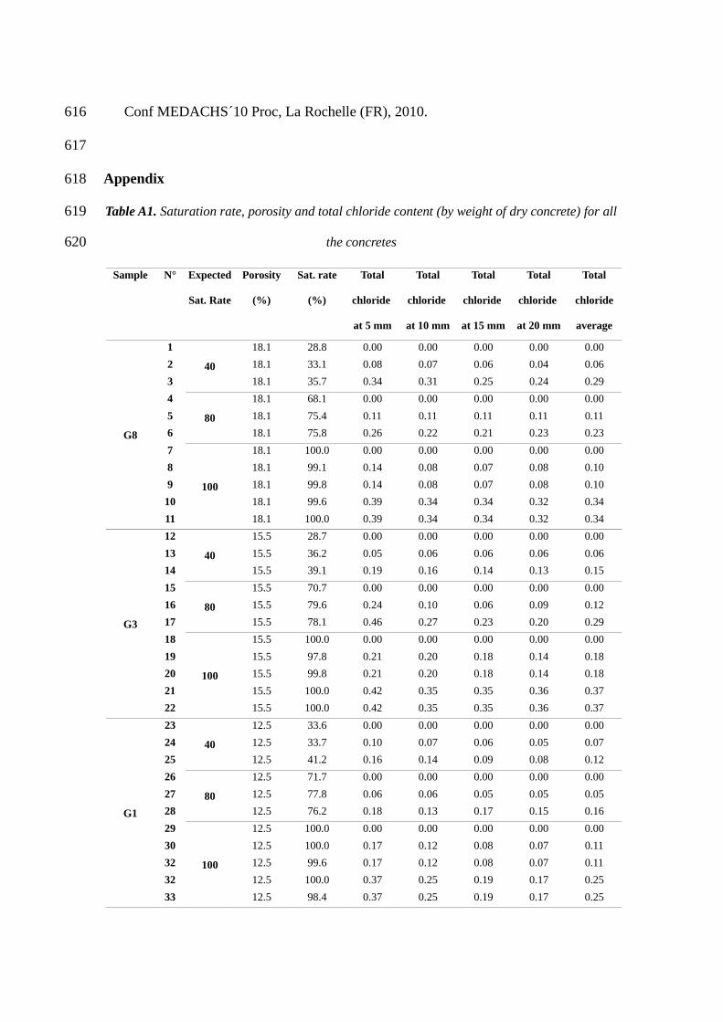
the sample samples. Table A1, in appendix, summarizes the saturation rate for all the

concretes, the porosity (measured on only 1 slab) and the total chloride content in

percentage weight of dry concrete, assessed by chemical titration at different depths (5,

10, 15 and 20 mm). It can be seen that there was no significant chloride gradient over

the depth investigated by titration.

2.2. NDT measurements

Radar technique

The radar techniques developed in the framework of this study relied on commercial

ground-penetrating radar (GPR) systems, using SIR-3000 systems from Geophysical

Survey Systems Inc. (GSSI®) and two separate ground-coupled 1.5 GHz antennas. Two

approaches were employed. One of them used four offsets (transmitter-receiver

distance), ranging from 7 to 14 cm, with an absorbing sponge placed between the

transmitter and the receiver, in order to measure the direct wave in the medium without

distortion due to the direct air wave [16]. Few observables were studied with this

94

95

96

97

98

99

100

101

102

103

104

105

106

107

108

109

110

111

112

113

114

115

116

117

configuration: the velocity, the corresponding relative permittivity and the attenuation

from the direct wave, and the arrival time for the largest offset. For the attenuation, the

observable studied corresponded to the slope coefficient of the logarithm of the

amplitudes.

The second approach, with one standard 1.5 GHz antenna, directly measured the peak-

to-peak amplitude of the direct wave in the medium [6-7]. This amplitude was

normalized to the peak-to-peak amplitude of the signal in air. For both configurations,

the coupled thickness of the medium, in the near vicinity of a GPR antenna which

interacts with it, can be estimated at 8-10 cm.

Capacitive technique

This technique, and the corresponding sensor, was designed by the network of

laboratories of the Ministry of Ecology, Sustainable Development and Energy (France)

and tested in reinforced concrete structures [16-18]. The principle of the capacitive

technique is to measure the resonance frequency of an oscillating circuit (around 30-35

MHz) between several electrodes lying on the upper face of the concrete slab. A

calibration allows the concrete relative permittivity ε'r to be obtained, which is mainly

related to the water content and the mixture components. The volume investigated

depends on the geometry of the electrodes (coupled depth of roughly 1-2 cm for

medium sized electrodes – ME – and 6-8 cm for large electrodes – GE).

Resistivity technique

The technique tested in this study used a four-probe square device that injects electrical

current between two lateral probes and measures the potential difference between the

118

119

120

121

122

123

124

125

126

127

128

129

130

131

132

133

134

135

136

137

138

139

140

141

other two probes [18-20]. The apparent resistivity is deduced from the ratio of the

potential to the intensity, according to the geometrical characteristics. Measurements,

with two spacings (5 and 10 cm), were performed for two orthogonal directions of

electrical current injection and then averaged, for coupling thicknesses of about 3 and 6

cm respectively. For an accurate analysis, given the wide range of variation of resistivity

between concretes in different states of moisture and chloride content, it is necessary to

study the resistivity in its logarithmic form (Log(Res)).

In the following text, the term “observable” will be used as a generic term for all the ND

studied observables (Table A2, in appendix).

3. Laboratory results

The first campaigns in the SENSO project showed that most of the NDT techniques

tended to give results that varied linearly with the indicators. As the EM techniques are

sensitive to both water and chloride content, and indirectly to the porosity, some

regression functions to one indicator can only be proposed when the other two are

constant. The data were processed to fit a multi-linear regression (3-parameter) function

on the three indicators, under the hypothesis of averaged values without depth gradient.

Equation 1, for the GPR velocity, is presented as a model equation:

(1)

where Poro, Sr and Cl- correspond to the porosity, the saturation rate and the chloride

content, respectively, and a, b, c and d to the multi-linear regression coefficients.

Some ND observables require specific adaptation, such as the GPR signal attenuation

and the resistivity measurements. Concerning the electrical resistivity, for concrete, as

for porous materials, the empirical Archie’s law is used and expressed as:

142

143

144

145

146

147

148

149

150

151

152

153

154

155

156

157

158

159

160

161

162

163

164

165

(2)

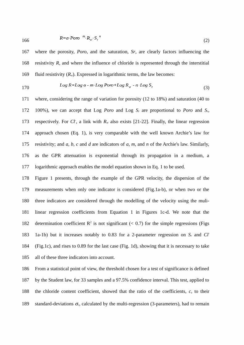
where the porosity, Poro, and the saturation, Sr, are clearly factors influencing the

resistivity R, and where the influence of chloride is represented through the interstitial

fluid resistivity (Rw). Expressed in logarithmic terms, the law becomes:

(3)

where, considering the range of variation for porosity (12 to 18%) and saturation (40 to

100%), we can accept that Log Poro and Log Sr are proportional to Poro and Sr,

respectively. For Cl-, a link with Rw also exists [21-22]. Finally, the linear regression

approach chosen (Eq. 1), is very comparable with the well known Archie’s law for

resistivity; and a, b, c and d are indicators of a, m, and n of the Archie's law. Similarly,

as the GPR attenuation is exponential through its propagation in a medium, a

logarithmic approach enables the model equation shown in Eq. 1 to be used.

Figure 1 presents, through the example of the GPR velocity, the dispersion of the

measurements when only one indicator is considered (Fig.1a-b), or when two or the

three indicators are considered through the modelling of the velocity using the muli-

linear regression coefficients from Equation 1 in Figures 1c-d. We note that the

determination coefficient R2 is not significant (< 0.7) for the simple regressions (Figs

1a-1b) but it increases notably to 0.83 for a 2-parameter regression on Sr and Cl-

(Fig.1c), and rises to 0.89 for the last case (Fig. 1d), showing that it is necessary to take

all of these three indicators into account.

From a statistical point of view, the threshold chosen for a test of significance is defined

by the Student law, for 33 samples and a 97.5% confidence interval. This test, applied to

the chloride content coefficient, showed that the ratio of the coefficients, c, to their

standard-deviations c, calculated by the multi-regression (3-parameters), had to remain

166

167

168

169

170

171

172

173

174

175

176

177

178

179

180

181

182

183

184

185

186

187

188

189

above the threshold 2.037.

With this approach for each ND method, the coefficients of the regression were assessed

as a function of porosity, saturation rate, and chloride content. For all the EM ND

techniques, values depended on the chloride contents assessed at different depths (5, 10,

15, 20 mm and average). Table 2 summarizes the values obtained in the test of

significance. The results confirm that all the EM ND techniques are sufficiently

sensitive and reliable as far as the estimation of the chloride content is concerned. We

note that the highest values (in bold in the table) are obtained when the depth of the

estimation of the chloride content tends to the coupled volume of the ND technique.

a) b)

c) d)

Fig. 1. GPR velocity measurements, obtained by CMP, as a function of a) the chloride content,

b) the saturation rate, c) the GPR velocity modelled using the 2-parameter regression (Sr and

Cl-), d) the GPR velocity modelled using the 3-parameter regression (Sr, Cl-, Poro)

Table 3 shows the regression coefficients obtained by keeping the case (depth for

estimation of chloride content) leading to the best value in the test of significance, for

190

191

192

193

194

195

196

197

198

199

200

201

202

203

each technique.

The values of the coefficients of the indicators, corresponding to Equation 1 and

presented in Table 3, enable the ND measurements to be linked to the modelled ones.

Some examples of modelling (one per technique) are shown in Figure 2. Their

coefficients of determination (R2) vary from 0.67 for the GPR (Time Offset-L parameter

observable) to 0.78 for the capacitive technique (LE), values which increase to above

0.8 when removing one apparent outlier. These results show that, even if the chloride

contents are not perfectly constant versus depth in the mixes, the multi-linear regression

remains efficient to estimate Cl-, while taking Sr and Poro into account.

Table 2. Values obtained in test of significance, applied to the Cl- coefficient, for the ND techniques

according to the chosen total chloride content (at 5, 10, 15 and 20 mm and average)

Test of significance values (> 2.037)

Technique Total

chloride

at 5 mm

Total

chloride

at 10 mm

Total

chloride

at 15 mm

Total

chloride

at 20 mm

Total

chloride

average

ResistivityQ5 5.25 5.04 5.03 5.33 5.34

Q10 4.31 4.10 4.23 4.53 4.41

CapacitiveAE 5.75 5.85 5.47 5.43 5.85

LE 6.22 6.31 6.08 6.38 6.51

GPR

Epsilon 3.50 4.44 5.24 5.66 4.64

Velocity 3.66 4.47 4.99 5.28 4.59

Log(peak-to-peak) 5.90 6.27 6.47 7.30 6.68

Ampl CMP 3.83 4.55 5.17 5.67 4.80

Ampl Offset-L 6.75 6.96 6.95 7.13 7.26

Time Offset-L 3.15 3.24 3.35 3.59 3.39

It is interesting to note that Hugenschmidt and Loser [8] obtained very similar values,

about 0.81 for the GPR attenuation (in logarithmic units), versus Cl-, using air-coupled 2

GHz echoes on concretes containing chlorides. These values are close to our coefficient

of 0.77 for Cl- for the GPR log (peak-to-peak) observable. Sbartaï & al. [23] also found

204

205

206

207

208

209

210

211

212

213

214

215

216

217

218

219

similar results, with a value of about 0.74, for the coefficient related to Cl-, using

ground-coupled GPR antennas at 1.5 GHz and a normalized reflected echo (in

logarithmic units), on homogeneous concrete slabs having 14-15 % porosity. This

means that several distinct and independent studies have led to the same reliability for

attenuation versus chloride content. This may be considered as a classical dependency.

Nevertheless, there is no discussion of uncertainties in these papers.

Table 3. Coefficient of the multi-regressions of the ND techniques performed in their optimal

configuration of chloride content (correponding to the greatest a/a)

Coefficients

Techniques

Coef. a for

Poro

Coef. b for

Sr

Coef. c for

Cl-

Coef. d R2 Chloride

content

ResistivityQ5 -0.167 -0.0083 -3.574 5.993 0.76 Average

Q10 -0.157 -0.0079 -3.383 5.637 0.73 20 mm

CapacitiveAE 1.037 0.0739 33.30 -8.559 0.72 10 mm

LE 0.612 0.0757 28.92 -3.527 0.78 Average

GPR

Epsilon 0.246 0.0519 9.628 1.600 0.85 20 mm

Velocity -0.105 -0.026 -3.397 13.45 0.89 20 mm

Log(peak-to-

peak)

-0.0125 -0.0007 -0.763 -0.077 0.77 20 mm

Ampl CMP -0.0015 -0.0003 -0.105 -0.0189 0.73 20 mm

Ampl Off.-L -0.0070 -0.0009 -0.227 0.308 0.87 Average

Time Off.-L 0.0181 0.00235 0.5245 0.788 0.67 20 mm

The influence of chlorides on electrical resistivity is complex since the interstitial fluids

in concrete are naturally conductive. Fluid in concrete depends on the composition of

the cement and additions, so it is influenced by alkali content: the more alkali there is in

the pore water, the smaller is the influence of external fluid [21]. The real value for Rw

in the Archie’s law is a composition of conductance of fluids from the concrete and

from external ingresses [24]. Numerous works present the relationship between

220

221

222

223

224

225

226

227

228

229

230

231

232

233

234

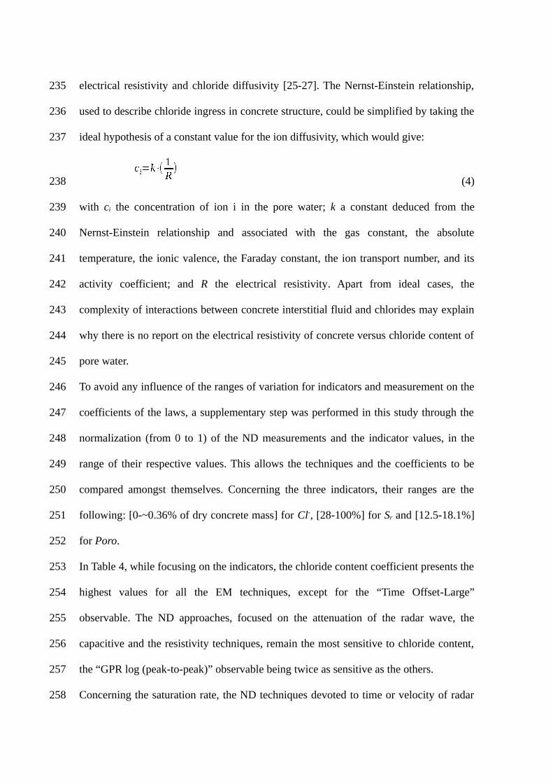
electrical resistivity and chloride diffusivity [25-27]. The Nernst-Einstein relationship,

used to describe chloride ingress in concrete structure, could be simplified by taking the

ideal hypothesis of a constant value for the ion diffusivity, which would give:

(4)

with ci the concentration of ion i in the pore water; k a constant deduced from the

Nernst-Einstein relationship and associated with the gas constant, the absolute

temperature, the ionic valence, the Faraday constant, the ion transport number, and its

activity coefficient; and R the electrical resistivity. Apart from ideal cases, the

complexity of interactions between concrete interstitial fluid and chlorides may explain

why there is no report on the electrical resistivity of concrete versus chloride content of

pore water.

To avoid any influence of the ranges of variation for indicators and measurement on the

coefficients of the laws, a supplementary step was performed in this study through the

normalization (from 0 to 1) of the ND measurements and the indicator values, in the

range of their respective values. This allows the techniques and the coefficients to be

compared amongst themselves. Concerning the three indicators, their ranges are the

following: [0-~0.36% of dry concrete mass] for Cl-, [28-100%] for Sr and [12.5-18.1%]

for Poro.

In Table 4, while focusing on the indicators, the chloride content coefficient presents the

highest values for all the EM techniques, except for the “Time Offset-Large”

observable. The ND approaches, focused on the attenuation of the radar wave, the

capacitive and the resistivity techniques, remain the most sensitive to chloride content,

the “GPR log (peak-to-peak)” observable being twice as sensitive as the others.

Concerning the saturation rate, the ND techniques devoted to time or velocity of radar

235

236

237

238

239

240

241

242

243

244

245

246

247

248

249

250

251

252

253

254

255

256

257

258

wave propagation are the most sensitive, slightly more than for the chloride content.

The difference between the capacitive technique and the GPR time or velocity can be

explained by the fact that the EM characteristics of civil engineering materials at the

frequencies used (very low GPR frequency band) are sensitive to both chloride and

water content [28], due to the predominant effect of interfacial polarization.

a) b)

c) d)

Fig. 2. Comparison of the measured and calculated observables for a) the resistivity technique

– quadripole 5 cm b) the capacitive technique – large electrodes, c) the GPR Log(peak-to-peak)

amplitude, d) the GPR amplitude (large offset), at their optimal configuration

Table 4. Coefficient of the multi-regressions of the ND normalized measurements performed in their

optimal configuration of chloride content (corresponding to the greatest a/a)

Coefficients obtained with normalized observables and

indicators

Techniques

Coef. a for Poro Coef. b for Sr Coef. c for Cl- Chloride

content

259

260

261

262

263

264

265

266

267

268

269

ResistivityQ5 -0.32 -0.20 -0.45 Average

Q10 -0.35 -0.23 -0.48 20 mm

CapacitiveAE 0.18 0.17 0.38 10 mm

LE 0.14 0.23 0.45 Average

GPR

Epsilon 0.15 0.4 0.37 20 mm

Velocity -0.15 -0.48 -0.31 20 mm

Log(peak-to-

peak)

-0.18 -0.12 -0.69 20 mm

Ampl CMP -0.11 -0.25 -0.49 20 mm

Ampl Off.-L -0.23 -0.39 -0.49 Average

Time Off.-L -0.20 -0.39 0.28 20 mm

Finally, for the porosity estimation, the electrical techniques give the best performance.

This can be explained by the increase in connectivity of pores as the porosity increases,

which facilitates ionic displacement and thus the electric current, especially for

saturation degrees higher than 40%.

This normalized study thus shows that all these EM techniques are capable of providing

information on the following indicators: chloride content, saturation rate and porosity, in

concrete mixes. Their sensitivity to these indicators encourages complementary use of

these ND techniques if we want to dissociate the indicators surveyed.

4. On-site implementation and discussion

The objective of the campaign described here is to estimate the uncertainty on the

values of indicators from ND measurements made at a real site in a tidal zone, using the

regressions studied above and the corresponding uncertainties (from the ND

measurement and from the regression). Given their high sensitivity to chlorides, three

techniques were considered for comparison, out of the three NDT families: resistivity,

capacity and GPR. By performing statistical calculations, this study, described below,

will quantify the influence of the ND measurements or the regressions on indicator

270

271

272

273

274

275

276

277

278

279

280

281

282

283

284

285

286

287

estimation, from a structural engineering point of view. As the calibration was not

performed on the structure in question, only the uncertainties will be studied, and not

the absolute values, for which no reliability estimate can be made.

4.1. Presentation of the site

The chosen test site was a 15-year-old reinforced concrete wharf at the port of Saint-

Nazaire (France). A large ND campaign was carried out on the site in the framework of

the SENSO project, in which all the authors participated. The wharf, the ND techniques,

and the destructive analysis are accurately described in [15] and EM values in [29].

The structure tested was a precast reinforced concrete beam exposed to chloride ingress

in a tidal zone. The concrete mix used a CEM II/A 32.5PM cement with a water-to-

cement ratio of 0.46, and included fly ash and siliceous aggregates as components. The

standard tests showed a 28-day compressive strength of about 36 MPa. Gas

permeability measurements on five cores gave values corresponding to a porosity in the

11-12% range, and chloride profiles were also obtained from these cores.

The chloride profiles, presented in [15], show values of total chlorides per weight of dry

concrete of about 0.025% in the first 5 mm, a maximum of 0.09+/-0.01% at 15+/-2 mm

and then a linear decrease to 0.03% at about 32 mm.

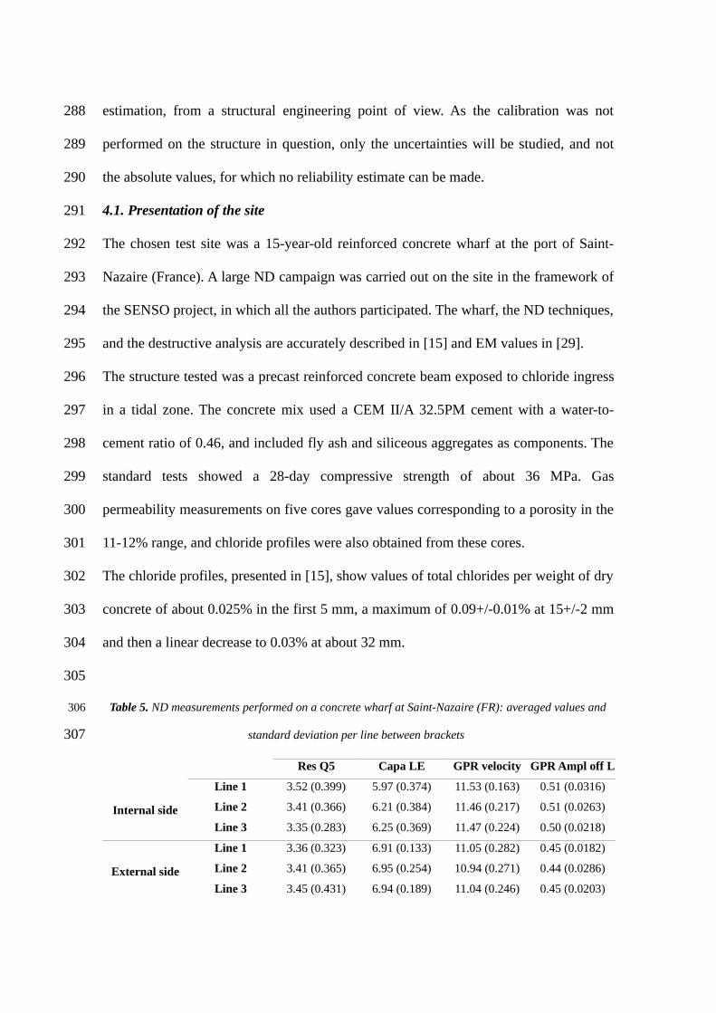
Table 5. ND measurements performed on a concrete wharf at Saint-Nazaire (FR): averaged values and

standard deviation per line between brackets

Res Q5 Capa LE GPR velocity GPR Ampl off L

Internal side

Line 1 3.52 (0.399) 5.97 (0.374) 11.53 (0.163) 0.51 (0.0316)

Line 2 3.41 (0.366) 6.21 (0.384) 11.46 (0.217) 0.51 (0.0263)

Line 3 3.35 (0.283) 6.25 (0.369) 11.47 (0.224) 0.50 (0.0218)

External side

Line 1 3.36 (0.323) 6.91 (0.133) 11.05 (0.282) 0.45 (0.0182)

Line 2 3.41 (0.365) 6.95 (0.254) 10.94 (0.271) 0.44 (0.0286)

Line 3 3.45 (0.431) 6.94 (0.189) 11.04 (0.246) 0.45 (0.0203)

288

289

290

291

292

293

294

295

296

297

298

299

300

301

302

303

304

305

306

307

NDT method S.D 0.012 0.0003 0.003 0.0055

ND measurements were performed on each side of the beam – the external side exposed

to wind, rain and ocean spray, and the protected, internal side under the wharf deck – on

three horizontal lines. Thirty measurements were recorded per face, at the centre of the

reinforcement meshes. The ND values shown in Table 5 are the average of each line. An

ND procedure repeated several times at one point (centre of a reinforced mesh) in order

to find the standard deviation (S.D.) of each NDT method on the structure (last line of

table 5).

4.2. Methodological approach

Non-destructive measurements led to the determination of the observables, from which

the indicators were deduced through the inverse analysis of a specific relationship for

each technique, for instance Eq.1. During this process, uncertainty appeared at various

levels, mainly (Table 6 based on Eq.1):

on the measurement (uncertainty on observable). This uncertainty was assessed

during the investigation of the structure by repeated measurements. For this

study, the measurement uncertainty is the standard deviation of repeated

measurements relative to the average value (in other words the Coefficient of

Variation CoV), given in terms of relative uncertainty;

on the relationship between observable and indicator (model error). This error is

linked to the reliability of the calibration process. In this study, it corresponds to

the standard error value of the parameter considered, as assessed during the

linear regression calculation relative to the average value of the parameter (the

CoV).

308

309

310

311

312

313

314

315

316

317

318

319

320

321

322

323

324

325

326

327

328

329

330

331

The sensitivity analysis showing the effect of these various uncertainty levels on

diagnostic reliability is performed through a Monte Carlo simulation. It consists of

performing repeated sampling for a parameter described by its statistics (average and

CoV). The simulated population respects the same statistical distribution. Then from

each “simulated uncertain term” of the population, it is possible assess the uncertainty

propagating to the final result. For this study, and at each step, 1000 values were

simulated. According to the objective, the uncertainties could be simulated on different

parameters.

Table 6. Uncertainty levels on Eq.1

parameter for instance in Eq.1 Symbol uncertainty uncertainty level

Observable Velocity GPR VGPR +/- VGPR measurement

law Porosity coefficient a +/- a calibration

law Saturation coefficient b +/- b calibration

law Chloride content coefficient c +/- c calibration

law Constant coefficient d +/- d calibration

indicator Porosity Poro +/- Poro interpretation

indicator Saturation rate Sr +/- Sr interpretation

indicator Chloride content Cl- +/- Cl- interpretation

If the measurement uncertainty is considered, with the perfect regression model, VGPR

exists, and a, b, c, d are equal to 0. Respectively one thousand “measured” values

are considered (statistically correct), leading to the calculation of a thousand values for

Poro, Sr and Cl- after inversion. Thus the average values can be assessed for each

indicator as well as Poro, Sr, and Cl-. If the measurement is considered as perfect

and the uncertainty is only on the regression model, VGPR equals 0, and a, b, c, d

exist. From measurements, and considering the thousand values each for a, b, c and d

(for the observable under consideration) to be statistically correct, a thousand values for

332

333

334

335

336

337

338

339

340

341

342

343

344

345

346

347

348

349

poro, Sr and Cl- are assessed by inversion. Here again, average values are assessed for

indicators and for Poro, Sr, and Cl-. Then, both approaches are studied and the

uncertainties on Poro, Sr and Cl- are compared.

Moreover, the inversion process is carried out considering matrix calculations (Eqs 5 to

7) with O the matrix of observables, d the matrix containing the constant term of each

regression, I the matrix of indicators, and M the matrix of regression coefficients.

Inversion consists to of determining the matrix [M]-1, inverse of [M], thus leading to the

assessment of its determinant: Det(M).

(5)

with

(6)

Inversion consists of assessing [M]-1 in order to solve the following equation:

(7)

This problem is not solvable if Det(M) is equal to 0, which would correspond to the

situation where the models have the same coefficients of regression. In this case, no

additional information would be provided by any NDT method compared with the

others. If Det(M) is very close to 0, the calculation error will be very high. To overcome

this difficulty it is decided to consider uncertainties of indicators, namely Poro, Sr,

and Cl- instead of the indicators themselves.

4.3. Influence of types of uncertainty of NDT methods

For this study, we considered the triplet: resistivity Q5, capa LE, and GPR velocity,

350

351

352

353

354

355

356

357

358

359

360

361

362

363

364

365

366

367

368

369

370

371

chosen as the three techniques presenting the best relationship to chloride content in

each of the three NDT families (see R² values in Table 3).

An overview of the results is given in the following tables (7, 8 and 9). Case 1

corresponds to ND values associated with their average standard deviation per line,

which includes a part of the material variability along the beam. Case 2 corresponds to

the standard deviation calculated at a measurement point, which corresponds to the

technique variability. Standard deviations decrease from roughly 40, 28, 23 and 2.4% in

case 1 to 1.2, 0.03, 0.3 and 0.55% in case 2 for res_Q5, capa_LE, GPR velocity and

GPR_Ampl_off_L, respectively.

The first observations in Tables 7 and 8 show that uncertainties on the regression

models lead to an unacceptable estimation of indicators. The models obtained from

laboratory experiments, which were not suited to Saint Nazaire wharf, are used. This is

made obvious by the negative values for chloride factors. So, the influence of model

error or measurement uncertainty is estimated by the error of indicator assessment and

not to by the value of the indicator. This implies that a calibration of the regression

models is necessary for each ND technique for every ND inspection on a new concrete

structure.

Table 7. Statistical inversions of the ND measurements, performed on a concrete wharf (Table 5), under

the hypothesis of perfect regression models or perfect measurements and considering Case 1

Perfect models (uncert. on meas.) Perfect measurements (uncert. on models)

Case 1 Porosity Sat Cl- Porosity Sat Cl-

Int. side

L1 14.3 (29%) 19.1 (65.3%) -0.025(306%) 19.2 (447%) 20.3 (768%) -0.17 (1569%)

L2 15.2 (26.2%) 19.7 (76.1%) -0.036 (217%) 20.4 (447%) 21.2 (773%) -0.19 (1460%)

L3 15.9 (19.1%) 18.1 (79.2%) -0.046 (143%) 21.2 (94.4%) 19.1 (882%) -0.21 (1426%)

Ext. side L1 15.2 (24.1%) 17.4 (46%) -0.060 (127%) 20.2 (433%) 42.2 (388%) -0.22 (1257%)

L2 14.7 (27.2%) 17.4 (37.6%) -0.070 (114%) 19.5 (429%) 50.0 (321%) -0.22 (1198%)

372

373

374

375

376

377

378

379

380

381

382

383

384

385

386

387

388

389

390

391

L3 14.0 (33.3%) 16.8 (40.4%) 0.044 (198%) 18.7 (433%) 44.5 (349%) -0.19 (1351%)

As inversions show similar results for the internal and the external sides, only the values

of the internal face are presented below.

Table 8. Statistical inversions of the ND measurements, performed on the internal side of the

concrete wharf (Table 5), under the hypothesis of perfect regression models or perfect

measurements and considering Case 2

Internal side Perfect models (uncert. on meas.) Perfect measurements (uncert. on models)

Porosity Sat Cl- Porosity Sat Cl-

Case 2

L1 14.4 (0.9%) 18.6 (1.6%) -0.026 (8.3%) 19.2 (447%) 20.3 (768%) -0.17 (1569%)

L2 15.3 (0.8%) 19.4 (1.6%) -0.038 (5.5%) 20.4 (447%) 21.2 (773%) -0.19 (1460%)

L3 15.9 (0.8%) 17.4 (1.7%) -0.044 (4.7%) 21.2 (94.4%) 19.1 (882%) -0.21 (1426%)

The analysis of Table 7 is mainly focused on the uncertainty values (percentage in bold

characters in brackets), and not on the values themselves, since the regression models

are not created on the surveyed concrete but on laboratory slabs. The first findings show

extremely high levels for Poro, Sr, and Cl- in the case of uncertainty of models, in a

range ten times above those for the case of uncertainty of measurements.

The second point concerns the comparison of cases 1 and 2 when considering perfect

models. We can note similar values of indicators but a large difference in the uncertainty

values. Taking account of the variability of ND measurements from a large zone (Case

1) on the inversion induces results that are unacceptable because unreliable. We must

consider only the uncertainty of the NDT on this concrete mix (obtained from the

repetitive procedure on one representative local zone) rather than the integrated

uncertainty combining NDT and the variability of the material.

Finally, from a structural engineering point of view, the uncertainties on the indicators

392

393

394

395

396

397

398

399

400

401

402

403

404

405

406

407

408

409

410

411

412

Poro, Sr, and Cl- give rise to acceptable ranges when the hypothesis of perfect

regression models is maintained (if they can be designed on the concrete being

surveyed) and when the standard deviation of each ND technique is found on site.

4.4. Influence of combination of observables

The choice of the three techniques also has an influence on uncertainties of assessment.

We compare the results obtained when the techniques were selected on their own

reliability with respect to chloride variations (as in Section 3, techniques chosen on the

R² value, see Table 3), or if the techniques were chosen according to their

complementarity (based on the assessment of the highest determinant value, see Eqs. 5

to 7).

The two cases are studied in Table 9, which shows the influence of observable

combination on the assessment of indicators. As expected, when the value of Det(M)

decreases too much, the inversion process induces unacceptable uncertainties, as seen

for the triplet Techn. Res (Q5) / Capa (LE) / GPR ampl.

Table 9. Statistical inversions of the ND measurements, performed on the internal side of the

concrete wharf (Table 5), including either the GPR velocity or the GPR amplitude

Perfect models (uncert. on meas.) Porosity Sat Cl-

Techn. Res / Capa / GPR vel.

Average S.D. per line

Det = -0.0464

Line 1 14.4 (0.9%) 18.6 (1.6%) -0.026 (8.3%)

Line 2 15.3 (0.8%) 19.4 (1.6%) -0.038 (5.5%)

Line 3 15.9 (0.8%) 17.4 (1.7%) -0.044 (4.7%)

Techn. Res / Capa / GPR ampl.

Off. L

Average S.D. per line

Det = -0.00092

Line 1 4.7 (4.5%) -849 (1.9%) 2.45 (1.8%)

Line 2 4.2 (5.0%) -965 (1.6%) 2.77 (1.6%)

Line 3 3.0 (6.9%) -1129 (5.9%) 3.23 (1.3%)

413

414

415

416

417

418

419

420

421

422

423

424

425

426

427

428

429

430

431

An explanation can be furnished by Figure 3, which shows the regression relations for

the two distinct NDT triplets (from Table 9) while focusing on chloride. Ideally, the

estimation of chloride content should be made by the intersection of the three

regressions. In both cases, there is no single intersection of the three curves.

Nevertheless, the uncertainty of the apparent solution (not exact since the calibration

does not correspond to the material under study) is represented by the band covered by

the three ranges of uncertainty for each of the observables.

The bandwidth of uncertainty on chloride content varies from less than 0.3 for the first

case (blue arrow in Fig. 3a), to more than 0.35 for the second case (blue arrow in Fig.

3b). The closer the three regressions intersect (the farther the determinant from Eq. 7 is

from 0) the less uncertainty there is. Then, for the second case, it is shown that both

resistivity and GPR amplitude have similar sensitivities to chloride (expressed by a

determinant very close to 0), and the third technique does not significantly improve the

assessment of indicator. For these two cases DET are -0.0464, and -0.0009, respectively.

a) b)

Fig. 3. Regressions of selected ND techniques (normalized values) versus chloride content for

the triplets a) Techn. Res (Q5) / Capa (LE) / GPR velocity and b) Techn. Res (Q5) / Capa (LE) /

GPR ampl. The bandwidths correspond to the uncertainties of each regression.

4.5. Discussion on how to choose an ideal third ND technique

432

433

434

435

436

437

438

439

440

441

442

443

444

445

446

447

448

449

450

451

The question of the choice of three complementary techniques could be then based on

the determinant value. To test this approach, and having already chosen the resistivity

and capacitive techniques, a third NDT is chosen: GPR epsilon, which leads to Det(M)

= 0.0721. The estimation of chloride content uncertainty with this new triplet (Fig. 4a)

is 0.35. This value is in the range of the first results, proving that this approach is not

sufficient when working with EM techniques.

Going further in this study, we also tested this criterion by considering an ideal virtual

technique fairly perpendicular to the first two (Fig. 4b). The uncertainty level of this

technique was taken to be in the same range as the others. The result shows a chloride

content uncertainty decreasing to 0.15. Finally, it should be noted that the uncertainty of

the ideal ND technique could strongly influence the uncertainty on indicators, even if

the intersection is quite perpendicular (that is to say, even if the determinant is high).

a) b)

Fig. 4. Regressions of selected ND techniques (normalized values) versus chloride content for

the triplets a) Techn. Res (Q5) / Capa (LE) / GPR eps and b) Techn. Res (Q5) / Capa (LE) /

ideal techn. The bandwidths correspond to the uncertainties of each regression.

5. Conclusion

The results presented in this paper concern the implementation of different NDT

methods (using radar, capacitive and resistivity techniques) for the detection of

452

453

454

455

456

457

458

459

460

461

462

463

464

465

466

467

468

469

470

471

chlorides in concrete. Three different concrete mixes were tested in the laboratory with

different levels of saturation and involving two concentrations of NaCl. A multi-linear

regression, depending on the three indicators: chloride content, saturation rate and

porosity, was performed for each ND technique, under the hypothesis of averaged

indicator values without a depth gradient.

The results show that all the techniques devoted to attenuation measurements or the

resistivity are very sensitive to the presence of chlorides. This phenomenon is less

visible for the relative permittivity, as the frequency increases in the GPR frequency

band. Concerning the other two indicators, more than half of the ND techniques are less

than half as sensitive to them as to the chloride content.

Experiments on a real site in a marine environment have shown that it is necessary to

take two other indicators into account: the saturation rate and the porosity, to properly

estimate the chloride content through a multi-linear regression approach. A statistical

study was performed on the influence of the accuracy of ND measurements and the

model error on chloride content, from a structural engineering point of view.

The principal results show that:

- all the ND techniques must be calibrated on the structure actually surveyed,

- the combination of 3 techniques sensitive to chloride is not necessarily the best ND

triplet,

- the determinant of the regression equations considered as an indicator of reliability

(for chloride estimation), is not sufficient because it is sensitive to the 3 techniques,

- when considering a virtual ideal technique (the regression slope of which would be

“perpendicular” to those of the other techniques), the parametric study shows the

importance of the uncertainty of each technique in the estimation of the chloride

472

473

474

475

476

477

478

479

480

481

482

483

484

485

486

487

488

489

490

491

492

493

494

495

content.

Finally, it is illusory to believe that it is possible to accurately estimate the chloride

content of a concrete structure using the hypothesis that all other indicators are spatially

constant. The paper has highlighted the present limitations of the various possible

approaches for chloride content assessment.

Acknowledgments

The French National Research Agency (ANR) is gratefully acknowledged for

supporting the ANR-PGCU SENSO project. This work is a contribution to COST action

TU1208 on “Civil engineering applications of GPR”.

Our thanks are extended to Susan Becker, a native English speaker, commissioned to

proofread the final English version of this paper.

Glossary

Chloride content: ratio (percentage) of the weight of total chloride (free and bound) to

the weight of dry concrete.

Durability indicator: property describing the concrete in term of durability and

performances (i.e. porosity, density, resistance, Young modulus, chloride content,

moisture...).

Indicator: generic term designating all durability indicators and more generally all the

properties involved in concrete durability

Multi-linear regression: approach of modeling the relationship between a dependent

variable (i.e. permittivity) and few conditioning variables (i.e. chloride content,

porosity...) using linear mathematical expression.

496

497

498

499

500

501

502

503

504

505

506

507

508

509

510

511

512

513

514

515

516

517

518

519

ND observable: direct value (i.e. permittivity, resistivity...) or extracted value (i.e. wave

attenuation or velocity…) from non-destructive (ND) measurements.

Porosity: ratio (in percentage) of the volume of void to the total volume of material.

Saturation rate: ratio (in percentage) of a volume of fluid (interstitial solution for

concrete) to the total volume of voids inside concrete.

uncertainty: statistical expression of the dispersion of a result, associated to the

imperfect and/or unknown information. For an inverse process to predict a value (ie.

Chloride content), it can result from both imperfect measurement and imperfect model.

Variability: expression characterizing the effect of the natural unmastered variations of

the material properties at the measurement scale. It leads to the dispersion of the

measurement results which can be attributed to the object (material) being measured.

References

[1] Baroghel-Bouny V, Belin P, Maultzsch M, Henry D. AgNO3 spray tests -

Advantages, weaknesses, and various applications to quantify chloride ingress into

concrete. Part 1: Non-steady-state diffusion tests in laboratory and exposure to

natural conditions. Mater Struct 2007;40:759-781.

[2] Tutti K. Corrosion of steel in Concrete. Research Report 4.82. Swed Cem

Concr Res Inst, Stockholm (SE), 1982.

[3] Kropp J, Alexander M. Non-destructive methods to measure ion migration. In:

RILEM Report 040 Non-destructive evaluation of the penetrability and thickness of

concrete cover. RILEM TC 189-NEC: State of the art report 2007;13-34.

[4] M. Torres-Luque M, Bastidas-Arteaga E, Schoefs F, Sánchez-Silva M, Osma

JF. Non-destructive methods for measuring chloride ingress into concrete: State-of-

520

521

522

523

524

525

526

527

528

529

530

531

532

533

534

535

536

537

538

539

540

541

542

543

the-art and future challenges. Constr Build Mater 2014;68:68-81.

[5] Soutsos MN, Bungey JH, Millard SG, Shaw MR, Patterson A. Dielectric

properties of concrete and their influence on radar testing. NDT&E Int

2001;34(6):419-25.

[6] Laurens S, Balayssac JP, Rhazi J, Arliguie G. Influence of concrete moisture

upon radar waveform. Mater Struct 2002;35(248):198–203.

[7] Klysz G, Balayssac JP. Determination of volumetric water content of concrete

using ground-penetrating radar. Cem Concr Res 2007;37(8):1164-71.

[8] Hugenschmidt J, Loser R. Detection of chlorides and moisture in concrete

structures with ground penetrating radar. Mater Struct 2008;41(4):785–92.

[9] Kalogeropoulos A, Van der Kruk J, Hugenschmidt J, Busch S, Merz K.

Chlorides and moisture assessment in concrete by GPR full waveform inversion.

Near Surf Geophys 2011;9(3):277-86.

[10] Villain G, Ihamouten A, du Plooy R, Palma Lopes S, Dérobert X. Use of

electromagnetic non-destructive techniques for monitoring water and chloride

ingress into concrete. Near Surf Geophys 2015;13:299-309.

[11] Loche JM, Lataste JF, Amiri O, Larget M, Tahlaiti M, Aït-Mokhtar A.

Evaluation of cover concrete and assessment of chloride ingress into cover concrete

by Non Destructive Testing. Part.I - Samples preparation - Porosity and resistivity

measurements. 1st Int Conf MEDACHS´08 Proc, Lisbon (PT), 2008.

[12] Dérobert X, Lataste JF, Loche JM, Villain G, Larget M, Aït-Mokhtar A, Amiri

O, Coffec O, Tahlaiti M, Durand O, Lu L, Abraham O. Evaluation of cover concrete

and assessment of chloride ingress into cover concrete by Non Destructive

Techniques. Part II – Comparison of NDT measurements and correlations. 1st Int

544

545

546

547

548

549

550

551

552

553

554

555

556

557

558

559

560

561

562

563

564

565

566

567

Conf MEDACHS´08 Proc, Lisbon (PT), 2008.

[13] Balayssac JP, Laurens S, Arliguie G, Breysse D, Garnier V, Dérobert X,

Piwakowski B. Description of the general outlines of the French project SENSO –

Quality assessment and limits of different NDT methods. Constr Build Mater

2012;35:131–8.

[14] Ploix MA, Garnier V, Breysse D, Moysan J. NDE data fusion to improve the

evaluation of concrete structures. NDT&E Int 2011;44(5):442-

8,doi:10.1016/j.ndteint.2011.04.006.

[15] Sbartaï ZM, Breysse D, Larget M, Balayssac JP. Combining NDT Techniques

for Improving Concrete Properties Evaluation. Cem & Conc Comp, 2012;34(6):725-

33.

[16] Villain G, Sbartaï ZM, Dérobert X, Garnier V, Balayssac JP. Durability

diagnosis of a concrete structure in a tidal zone by combining NDT methods:

laboratory tests and case study. Constr Build Mater 2012;37:893–903.

[17] Dérobert X, Iaquinta J, Klysz G, Balayssac JP. Use of capacitive and GPR

techniques for non-destructive evaluation of cover concrete. NDT&E Int

2008;41(1):44-52.

[18] Chataigner S, Saussol JL, Dérobert X, Villain G. Temperature influence on

electromagnetic measurements of concrete moisture", Eur Journ Env & Civil Eng

2015;19(4):482-95,http://dx.doi.org/10.1080/19648189.2014.960102.

[19] Lataste JF, Sirieix C, Breysse D, Frappa M. Electrical resistivity measurement

applied to cracking assessment on reinforced concrete structures in civil

engineering. NDT&E Int 2003;36(6):383-94.

[20] Lataste JF, de Larrard T, Benboudjema F, Semenadisse J. Study of electrical

568

569

570

571

572

573

574

575

576

577

578

579

580

581

582

583

584

585

586

587

588

589

590

591

resistivity: variability assessment on two concretes: protocol study in laboratory and

assessment on site. Eur Journ Env & Civil Eng 2012;16(3-4):298-310.

[21] Hunkeler F. The resistivity of pore-water solution - a decisive parameter of

rebar corrosion and repair methods. Constr Build Mater 1996;10(5):381-9.

[22] Saleem M, Shameem M, Hussain SE, Maslehuddin M. Effect of moisture,

chloride, and sulfate contamination on the electrical resistivity of Portland Cement

Concrete. Constr Build Mater 1996;10(3):209-14.

[23] Sbartaï ZM, Laurens S, Balayssac JP, Arliguie A, Ballivy G. Ability of the

direct wave of radar ground-coupled antenna for NDT of concrete structures.

NDT&E Int 2006;39:400-7.

[24] McCarter WJ, Ezirim H, Emerson M. Properties in the cover zone :Water

penetration, sorptivity and ionic ingress. Mag Concr Res 1996;48(176):149-56.

[25] Andrade C, Andrea R, Rebolledo N. Chloride ion penetration in concrete: the

reaction factor in the electrical resistivity model. Cem Concr Comp 2014;47:41-6.

[26] Polder RB, Peelen WHA. Characterisation of chloride transport and

reinforcement corrosion in concrete under cyclic wetting and drying by electrical

resistivity. Cem Concr Res 2002;24:427-35.

[27] Sengul O. Used of electrical resistivity as an indicator for durability. Constr

Build Mater 2014;73:434-41.

[28] Dérobert X, Villain G, Cortas R, Chazelas JL. EM characterization of

hydraulic concretes in the GPR frequency-band using a quadratic experimental

design. 7th Int Symp NDT-CE Proc, Nantes (FR), 2009.

[29] Balayssac JP, Laurens S, Lataste JF, Dérobert X. Evaluation of chloride

contamination in concrete by combining non destructive testing methods. 2nd Int

592

593

594

595

596

597

598

599

600

601

602

603

604

605

606

607

608

609

610

611

612

613

614

615

Conf MEDACHS´10 Proc, La Rochelle (FR), 2010.

Appendix

Table A1. Saturation rate, porosity and total chloride content (by weight of dry concrete) for all

the concretes

Sample N° Expected

Sat. Rate

Porosity

(%)

Sat. rate

(%)

Total

chloride

at 5 mm

Total

chloride

at 10 mm

Total

chloride

at 15 mm

Total

chloride

at 20 mm

Total

chloride

average

G8

1

40

18.1 28.8 0.00 0.00 0.00 0.00 0.00

2 18.1 33.1 0.08 0.07 0.06 0.04 0.06

3 18.1 35.7 0.34 0.31 0.25 0.24 0.29

4

80

18.1 68.1 0.00 0.00 0.00 0.00 0.00

5 18.1 75.4 0.11 0.11 0.11 0.11 0.11

6 18.1 75.8 0.26 0.22 0.21 0.23 0.23

7

100

18.1 100.0 0.00 0.00 0.00 0.00 0.00

8 18.1 99.1 0.14 0.08 0.07 0.08 0.10

9 18.1 99.8 0.14 0.08 0.07 0.08 0.10

10 18.1 99.6 0.39 0.34 0.34 0.32 0.34

11 18.1 100.0 0.39 0.34 0.34 0.32 0.34

G3

12

40

15.5 28.7 0.00 0.00 0.00 0.00 0.00

13 15.5 36.2 0.05 0.06 0.06 0.06 0.06

14 15.5 39.1 0.19 0.16 0.14 0.13 0.15

15

80

15.5 70.7 0.00 0.00 0.00 0.00 0.00

16 15.5 79.6 0.24 0.10 0.06 0.09 0.12

17 15.5 78.1 0.46 0.27 0.23 0.20 0.29

18

100

15.5 100.0 0.00 0.00 0.00 0.00 0.00

19 15.5 97.8 0.21 0.20 0.18 0.14 0.18

20 15.5 99.8 0.21 0.20 0.18 0.14 0.18

21 15.5 100.0 0.42 0.35 0.35 0.36 0.37

22 15.5 100.0 0.42 0.35 0.35 0.36 0.37

G1

23

40

12.5 33.6 0.00 0.00 0.00 0.00 0.00

24 12.5 33.7 0.10 0.07 0.06 0.05 0.07

25 12.5 41.2 0.16 0.14 0.09 0.08 0.12

26

80

12.5 71.7 0.00 0.00 0.00 0.00 0.00

27 12.5 77.8 0.06 0.06 0.05 0.05 0.05

28 12.5 76.2 0.18 0.13 0.17 0.15 0.16

29

100

12.5 100.0 0.00 0.00 0.00 0.00 0.00

30 12.5 100.0 0.17 0.12 0.08 0.07 0.11

32 12.5 99.6 0.17 0.12 0.08 0.07 0.11

32 12.5 100.0 0.37 0.25 0.19 0.17 0.25

33 12.5 98.4 0.37 0.25 0.19 0.17 0.25

616

617

618

619

620

Table A2. ND measurements

Sample N° Capa

(LE)

(-)

Capa

(ME)

(-)

Log (Res

– 5 cm)

(.m)

Log (Res

– 10 cm)

(.m)

GPR

velocity

(cm/ns)

GPR pic-

pic

(-)

Log(GPR

att.)

(-)

GPR

Ampl

(D4) - (-)

GPR OD

(D4)

(ns)

G8

1 7.07 7.34 3.32 2.97 11.35 0.543 -0.054 0.154 1.104

2 12.82 16.34 2.60 2.73 10.71 0.520 -0.055 0.165 1.220

3 17.53 22.64 1.95 1.94 10.00 0.320 -0.066 0.100 1.330

4 10.84 12.31 2.67 2.35 9.77 0.447 -0.063 0.115 1.261

5 21.14 24.11 1.37 1.36 9.23 0.310 -0.077 0.071 1.410

6 22.86 25.36 1.54 1.56 9.11 0.310 -0.095 0.045 1.430

7 13.67 15.50 1.97 1.80 8.89 0.429 -0.065 0.104 1.463

8 16.53 19.44 2.03 2.10 8.57 0.410 -0.084 0.052 1.260

9 21.05 23.44 1.78 1.78 8.60 0.320 -0.084 0.049 1.330

10 22.93 37.65 1.13 1.16 7.87 0.220 -0.088 0.028 1.540

11 16.12 17.26 1.27 1.17 7.88 0.250 -0.105 0.023 1.510

G3

12 6.92 7.52 3.58 3.25 11.01 0.547 -0.058 0.181 1.112

13 11.39 13.15 2.74 2.83 10.67 0.510 -0.053 0.155 1.190

14 12.20 16.08 1.71 1.72 10.76 0.350 -0.052 0.166 1.300

15 11.08 12.58 2.32 2.04 9.56 0.430 -0.071 0.142 1.285

16 18.34 21.68 1.53 1.52 9.43 0.350 -0.073 0.082 1.380

17 21.95 23.29 1.49 1.35 9.03 0.300 -0.080- 0.056 1.420

18 13.85 16.19 2.07 1.84 8.61 0.421 0.061 0.120 1.420

19 19.72 19.71 2.70 2.74 8.64 0.550 -0.101 0.041 1.180

20 22.43 24.34 1.56 1.57 8.39 0.340 -0.092 0.040 1.310

21 29.90 27.76 1.03 1.03 7.45 0.220 -0.125 0.012 1.520

22 24.74 23.17 1.06 1.02 7.72 0.250 -0.121 0.017 1.500

G1

23 6.15 5.86 3.94 3.38 11.27 0.537 -0.064 0.158 0.878

24 11.04 12.38 3.37 3.50 10.23 0.460 -0.060 0.129 1.210

25 11.04 13.52 2.85 2.82 10.20 0.440 -0.049 0.155 1.240

26 8.02 7.59 3.52 3.22 10.30 0.475 -0.066 0.166 1.196

27 12.35 12.96 2.52 2.51 9.97 0.410 -0.059 0.129 1.210

28 12.62 14.09 2.68 2.64 9.95 0.490 -0.060 0.126 1.270

29 10.75 11.17 3.28 3.06 9.55 0.511 -0.057 0.155 1.347

30 15.02 15.85 3.42 3.52 9.76 0.490 -0.067 0.115 1.230

32 13.65 15.40 2.95 3.01 9.76 0.470 -0.067 0.115 1.300

32 17.14 17.75 2.25 2.27 9.36 0.380 -0.071 0.079 1.290

33 16.19 18.62 2.44 2.41 9.58 0.430 -0.070 0.096 1.300

621

622

623

624

625