evaluation of base ground - sace.ktu.lt

Journal of Sustainable Architecture and Civil Engineering 2016/1/1460

Journal of Sustainable Architecture and Civil EngineeringVol. 1/ No. 14 / 2016pp. 60-72DOI 10.5755/j01.sace.14.1.15821 © Kaunas University of Technology

Received 2016/03/24

Accepted after revision 2016/05/31

Evaluation of Base Ground Stiffness on Statically Indeterminate Framed Building Structures

JSACE 1/14 Evaluation of Base Ground Stiffness on Statically Indeterminate Framed Building Structures

*Corresponding author: [email protected]

http://dx.doi.org/10.5755/j01.sace.14.1.15821

Introduction

Ignacio Villalon*, Deividas Martinavičius, Mindaugas Gricius, Šarūnas Kelpša Department of Building Structures, Faculty of Civil Engineering and Architecture Kaunas University of Technology, Studentu st. 48, LT-51367 Kaunas, Lithuania

Mindaugas KasiulevičiusJSC “Smailusis skliautas”, Piliakalnio st. 3, LT-46224 Kaunas, Lithuania

The aim of this paper is to investigate the influence of the modulus of subgrade reaction in statically indeterminate framed structures. In building’s design the interaction between ground and foundation can be modelled variously: using springs instead of supports, modelling the wholesale soil as finite elements, etc. The most common situation in practice is that the interaction is modelled using the springs. Nevertheless, there is not just one approved method to calculate it, and engineers use different methods, proposed by various authors. In practice the settlements of foundations are usually calculated and compared with the limit value. However, in some cases the impact of settlements is not taken into account on the analysis of the structure. During the design process, the number of boreholes is always limited. Therefore, the real situation cannot be considered exactly. As a result, unforeseen settlements may cause the considerable redistribution of internal forces, leading to the cracking or even to the failure of the structure.In this research, different calculation methods of modulus of subgrade reaction are presented. Most of these methods are adopted for the base of foundations consisted of one soil layer. Therefore, an evaluation proposal of the modulus of subgrade reaction for multi-layered soils, using the reviewed methods, is suggested. Using those methods, the modulus of subgrade reaction of soils of 4 specific boreholes were calculated and compared. Furthermore, internal forces of two-storied framed building were calculated and compared in two different cases. In the first case the calculations are performed considering the settlements of the foundations. The settlements are calculated using 2 particular geological situations. In the second case all supports are assumed to be rigid.

KEYWORDS: base ground, modulus subgrade reaction, settlements, redistribution of internal forces.

The settlements of the foundations are a very significant factor, which affects the behaviour of structures of the designed building. If the settlements in the design process are not evaluated accurately, it may cause undesirable effects for the elements of the buildings: cracks and con-siderable deformations may occur in the constructions. The whole structure may even collapse. Therefore, evaluation of those settlements is a substantial stage in the design process. Different standards and recommendations, which limit the settlements of foundations exist. It is determined in appendix H of EN-1997-1:2004: Eurocode 7 (further – EC7) that for structures with individual foundations, the settlements up to 50 mm are acceptable. EC7 and other authors (eg. Skempton and McDonald (1956), Polshin and Tokar (1957), Bjerrum (1963) and others) also limit the ratio of

61Journal of Sustainable Architecture and Civil Engineering 2016/1/14

settlements of adjacent foundations, because when the foundations settle irregularly, additional dangerous internal forces in the structures may be caused.

On purpose to predict and avoid the negative effects of settlements of foundations, in the design process it is very important to describe and evaluate the interaction of soil particularly accurately. The mechanical behaviour of soil is very complex because of its nonlinear, heterogeneous and stress dependent nature. Therefore, in the modelling of soil, frequently particular assumptions are admitted, simplifying the complex mechanical behaviour of soil. One of the most important assumptions is Winkler’s (1867) suggested model. Winkler’s (1867) local elastic deformations theory describes the soil as a spring, which has a particular stiffness. That stiffness is named the modulus of subgrade reaction ks and is one of the most significant magnitudes in the calculation of the settlements of foundations. It is a conceptual magnitude, which describes the ratio between applied load and the subsequent deformation of soil (Bowles 1997).

The main issue of Winkler’s model is the calculation of the modulus of subgrade reaction ks. One of the first experiments which was made on purpose to obtain this magnitude was performed by Terzaghi (1955), by loading the subgrade with a metal plate. However, these experimental results are not sufficiently accurate because of the fact that modulus of subgrade reaction depends not only on properties of soil, but also on the magnitude of load and geometrical parameters of the foundation, whereas these conditions are hardly achievable while performing the experiment with metal plates. As Ziaie-Moayed and Janbaz (2009) observed, the method of Terzaghi becomes in-accurate when dimensions of foundations are much greater than dimensions of the plate.

The modulus of subgrade reaction depends on various factors: the width of foundation’s base (B), shape, the thickness of base, depth (D), the elastic modulus of material of foundation’s base (Ef) and the moment of inertia (If), Poisson’s ratio of soil (ν), the load which press the soil, the soil deformation modulus (E0) and etc. The shear deformation (Poisson’s) coefficient of soil describes the ratio between shear and normal stresses. The tentative magnitudes of this coefficient may be chosen by Rowe’s (2001) represented proposals: for clay in undrained conditions – 0,5; for clay in drained conditions – 0,2-0,3; for thick sand – 0,3-0,4; for powdery sand – 0,1-0,3.

The modulus of subgrade reaction is a useful magnitude in modelling of foundations and subgrade interaction. As mentioned above, it does not depend on “internal” factors as the natural properties of soil, but also on “external” factors such as the geometrical characteristics of foundation or the magnitude of loading. For this reason, the modulus of subgrade reaction is not a fundamental property of soil. Depending on the mentioned external factors, for the same soil, the coefficient ks may obtain different magnitudes. There does not exist a united calculation method of the modulus of subgrade reaction. Therefore, the comparable analysis of different calculation methods was performed. Further, ten different methods of calculation of coefficient ks are analysed and evalu-ated according to its accuracy.

Moreover, an influence of different settlements of foundations for structures is assessed. A com-parable analysis of redistribution of the internal forces of the modelled constructional elements of the structure is performed by a computer-based program. The analysis consists of comparing the redistribution of internal forces when the settlements of all foundations are the same and the case where the settlements are different.

Calculation methods

The first analysed method is the Winkler´s model. This model describes the soil as an elastic system in which there is a linear dependence between the applied load and the subsequent settle-ments of the foundation. The mathematical value which describes this dependence, is the modu-lus subgrade reaction ks:

where: F– applied load to the soil; s – foundation settlement.

(1)sFks =


In order to determine the modulus subgrade reaction ks, the value of the settlement of the foun-dation (method No. 1) must be previously obtained. There are different ways to calculate these settlements. In this case, the method of addition was used, where the total settlement of the soil consists of the deformation of each small layer in which the soil is divided.

Using the principles of the elastic theory F. Schleicher (1926) presented a mathematical expres-sion to calculate the modulus subgrade reaction (method No. 2):

Vesic (1961) considered the influence of the materials and the section of the foundation and pro-posed an expression to obtain ks (method No. 3):

where: ω – form coefficient of the foundation (for squared elastic foundation slabs – ω=0,95; for squared rigid foundation slabs – ω=0,88); E0 – deformation modulus of soil.

where: Ef – elastic modulus of foundation; If – moment of inertia of the section of the foundation.

(2)

Using the principles of the elastic theory F. Schleicher (1926) presented a mathematical expression to calculate the modulus subgrade reaction (method No. 2):

(2)


Vesic (1961) considered the influence of the materials and the section of the foundation and proposed an expression to obtain ks (method No. 3):

(3)

The value ks’ can be obtained using the next equation

2012

40'

165,0

E

IEBEk

ffs (4)

where: – elastic modulus of foundation; – moment of inertia of the section of the foundation. For practical purpose Vesic reduces the expression to (method No. 4):

(5)

According to Timoshenko and Goodyear (1951) method to calculate foundation settlements,

J. Bowles (1997) proposed another equation to obtain ks (method No. 5):

(6)

where: IF – influence factor, which depends on the ratio D/L and L/B (L– foundation length; B– foundation width; D – foundation slab depth) and on Poisson’s ratio ν;

IS – influence factor, which depends on L’/B’ ratio (L’ and B’ – effective foundation dimensions), width of the soil layer, Poisson’s coefficient ν and depth of the foundation D.

m – number of corners contributing to settlement (at a corner of the footing m=1; at the centre m=4).

In all of the presented methods modulus subgrade reaction ks is obtained from soil deformation

modulus E0. However, this property sometimes is not known. Therefore, it can be useful to count on other kind of approximations not depending on E0. J. Bowles (1997) proposed a method in which modulus subgrade reaction ks can be obtained from the allowable bear capacity of the soil qa (method No. 6):

(7) where: SF – safe factor; qa – allowable bear capacity.

Selvadurai (1984) proposed another method to obtain ks (method No. 7):

(8)

Modulus ks can be obtained using finite-element analysis software Autodesk Robot Structural Analysis Professional (further – Autodesk Robot) (method No. 8). This program obtains ks by predicting the settlements of a footing by the method of addition (which is used in the method No. 1).

20

1-νBωEks

B'kk s

s

fE fI

1...650 12 ,

ks E0

B 1 v2

FSs IImνB

EΔHΔqk

2

0

1

as qSFk 40

20

1650

νBE,

ks

(3)



(2)



(3)


2012

40'

165,0

E

IEBEk

ffs (4)


(5)



(6)








(8)


20

1-νBωEks

B'k

k ss

fE fI

1...650 12 ,

ks E0

B 1 v2

FSs IImνB

EΔHΔqk

2

0

1

as qSFk 40

20

1650

νBE,ks

For practical purpose Vesic reduces the expression


(2)



(3)


2012

40'

165,0

E

IEBEk

ffs (4)


(5)



(6)








(8)


20

1-νBωEks

B'kk s

s

fE fI

1...650 12 ,

ks E0

B 1 v2

FSs IImνB

EΔHΔqk

2

0

1

as qSFk 40

20

1650

νBE,

ks

to (method No. 4):

(4)


(2)



(3)


2012

40'

165,0

E

IEBEk

ffs (4)


(5)



(6)








(8)


20

1-νBωEks

B'kk s

s

fE fI

1...650 12 ,

ks E0

B 1 v2

FSs IImνB

EΔHΔqk

2

0

1

as qSFk 40

20

1650

νBE,ks

(5)

(6)


(2)



(3)


2012

40'

165,0

E

IEBEk

ffs (4)


(5)



(6)








(8)


20

1-νBωEks

B'kk s

s

fE fI

1...650 12 ,

ks E0

B 1 v2

FSs IImνB

EΔHΔqk

2

0

1

as qSFk 40

20

1650

νBE,ks

According to Timoshenko and Goodyear (1951) method to calculate foundation settlements, J. Bowles (1997) proposed another equation to obtain ks (method No. 5):


(2)



(3)


2012

40'

165,0

E

IEBEk

ffs (4)


(5)



(6)








(8)


20

1-νBωEks

B'kk s

s

fE fI

1...650 12 ,

ks E0

B 1 v2

FSs IImνB

EΔHΔqk

2

0

1

as qSFk 40

20

1650

νBE,

ks

where:

IF – influence factor, which depends on the ratio D/L and L/B (L– foundation length; B– foundation width; D – foundation slab depth) and on Poisson’s ratio ν;




where: SF – safe factor; qa – allowable bear capacity.

In all of the presented methods modulus subgrade reaction ks is obtained from soil deformation modulus E0. However, this property sometimes is not known. Therefore, it can be useful to count on other kind of approximations not depending on E0. J. Bowles (1997) proposed a method in which modulus subgrade reaction ks can be obtained from the allowable bear capacity of the soil qa (method No. 6):

(7)



(2)



(3)


2012

40'

165,0

E

IEBEk

ffs (4)


(5)



(6)








(8)


20

1-νBωEks

B'kk s

s

fE fI

1...650 12 ,

ks E0

B 1 v2

FSs IImνB

EΔHΔqk

2

0

1

as qSFk 40

20

1650

νBE,ks

(8)

Modulus ks can be obtained using finite-element analysis software Autodesk Robot Structural Analysis Professional (further – Autodesk Robot) (method No. 8). This program obtains ks by pre-dicting the settlements of a footing by the method of addition (which is used in the method No. 1).

Another way to determine modulus of subgrade reaction is to apply the finite layer method. It is assumed that, under a footing, there are vertical shear forces between the particles of the soil, so that the soil behaves plastically. However, going deeper in the ground, it occurs that these shear forces become weaker and, at some depth, disappear. Then, the considered soil behaves elastically. This means that there is a layer under the footing of thickness Hsl in which there are plastic deformations. It is recommended to take Hsl=1/4 B. The results obtained by some authors (Gorbunov-Posadov et al. (1984), Zhemochkin B. N. and Sinitsyn A. P. (1947)) are provided in (8) and (9) equations:


(2)



(3)


2012

40'

165,0

E

IEBEk

ffs (4)


(5)



(6)








(8)


20

1-νBωEks

B'kk s

s

fE fI

1...650 12 ,

ks E0

B 1 v2

FSs IImνB

EΔHΔqk

2

0

1

as qSFk 40

20

1650

νBE,

ks

(9)

(10)

The first equation (Eq. 9) considers that the plastic layer can slide on the ground, which is under it (method No. 9); the other equation assumes that slip does not occur (method No. 10).


(9)

(10)

The first equation (Eq. 9) considers that the plastic layer can slide on the ground, which is

under it (method No. 9); the other equation assumes that slip does not occur (method No. 10).

Calculation of modulus subgrade reaction for a multi-layer soil In most of analysed methods, modulus ks depends on other ground properties like deformation

modulus E0, Poisson’s coefficient ν and bear capacity qa. When under the footing is a one-layered soil, these properties are assumed be uniform and the modulus ks can be obtained simply using the considered methods.

Nevertheless, frequently ground consists of several layers with different type of soil, mechanical properties, granulometric composition, thickness, water saturation degree and etc. Therefore, in order to calculate modulus subgrade reaction using the analysed methods and considering these different properties between soil layers, authors propose to apply the influence factor ki to each soil layer. This coefficient depends on the thickness and the depth of the considered layer. The thinner and deeper layer is the less significant layer. The influence factor ki also depends on the deformation modulus E0 of the layer and on the form and dimensions of the foundation.

First of all transitional coefficient ktr,i is obtained:

(11)

where: L1 – half of the length of the foundation; B1 – half of the foundation width; zi – upper depth of the considered layer.

(12) The transitional coefficient may be obtained from the tables presented by some authors (e. g.,

Šližytė et al. (2012)). In this case ktr,i can be selected from the ratio between foundation and from the relative depth of the analysed layer .

Transitional coefficients ktr,i are normalized and the influence factor of layer is obtained:

(13)

The final joint properties of the overall multi-layered soil are calculated by these equations:

(14)

sls Hν

Ek

2

0

1

sl

s HννEνk

211

1 0

22

122

1

112

12

122

221

2111

0

arcsin2

iii

ii

i,

iitr,

zBzL

BLBLzDD

zBLzBLEh

k

21

21

21 zBLD

L/Bη z/Bζ 2

ki ktr,i

ktr,ii1

n

n

i,ii EkE

100


(9)

(10)







(11)





(13)


(14)

sls Hν

Ek

20

1

sl

s HννEνk

211

1 0

22

122

1

112

12

122

221

2111

0

arcsin2

iii

ii

i,

iitr,

zBzL

BLBLzDD

zBLzBLEh

k

21

21

21 zBLD

L/Bη z/Bζ 2

ki ktr,i

ktr,ii1

n

n

i,ii EkE

100

In most of analysed methods, modulus ks depends on other ground properties like deformation modulus E0, Poisson’s coefficient ν and bear capacity qa. When under the footing is a one-layered soil, these properties are assumed be uniform and the modulus ks can be obtained simply using the considered methods.

Nevertheless, frequently ground consists of several layers with different type of soil, mechanical properties, granulometric composition, thickness, water saturation degree and etc. Therefore, in order to calculate modulus subgrade reaction using the analysed methods and considering these different properties between soil layers, authors propose to apply the influence factor ki to each soil layer. This coefficient depends on the thickness and the depth of the considered layer. The

Calculation of modulus subgrade reaction for a multi-layer soil


thinner and deeper layer is the less significant layer. The influence factor ki also depends on the deformation modulus E0 of the layer and on the form and dimensions of the foundation.


(11)

The transitional coefficient may be obtained from the tables presented by some authors (e. g., Šližytė et al. (2012)). In this case ktr,i can be selected from the ratio between foundation


(9)

(10)







(11)





(13)


(14)

sls Hν

Ek

20

1

sl

s HννEνk

211

1 0

22

122

1

112

12

122

221

2111

0

arcsin2

iii

ii

i,

iitr,

zBzL

BLBLzDD

zBLzBLEh

k

21

21

21 zBLD

L/Bη z/Bζ 2

ki ktr,i

ktr,ii1

n

n

i,ii EkE

100

and from the relative depth of the analysed layer


(9)

(10)







(11)





(13)


(14)

sls Hν

Ek

20

1

sl

s HννEνk

211

1 0

22

122

1

112

12

122

221

2111

0

arcsin2

iii

ii

i,

iitr,

zBzL

BLBLzDD

zBLzBLEh

k

21

21

21 zBLD

L/Bη z/Bζ 2

ki ktr,i

ktr,ii1

n

n

i,ii EkE

100

.



(9)

(10)







(11)





(13)


(14)

sls Hν

Ek

20

1

sl

s HννEνk

211

1 0

22

122

1

112

12

122

221

2111

0

arcsin2

iii

ii

i,

iitr,

zBzL

BLBLzDD

zBLzBLEh

k

21

21

21 zBLD

L/Bη z/Bζ 2

ki ktr,i

ktr,ii1

n

n

i,ii EkE

100

where:

L1 – half of the length of the foundation; B

1 – half of the foundation width;

zi – upper depth of the considered layer.

(12)

(14)

(15)

(16)


(9)

(10)







(11)





(13)


(14)

sls Hν

Ek

20

1

sl

s HννEνk

211

1 0

22

122

1

112

12

122

221

2111

0

arcsin2

iii

ii

i,

iitr,

zBzL

BLBLzDD

zBLzBLEh

k

21

21

21 zBLD

L/Bη z/Bζ 2

ki ktr,i

ktr,ii1

n

n

i,ii EkE

100

(13)



(9)

(10)







(11)





(13)


(14)

sls Hν

Ek

20

1

sl

s HννEνk

211

1 0

22

122

1

112

12

122

221

2111

0

arcsin2

iii

ii

i,

iitr,

zBzL

BLBLzDD

zBLzBLEh

k

21

21

21 zBLD

L/Bη z/Bζ 2

ki ktr,i

ktr,ii1

n

n

i,ii EkE

100


(9)

(10)







(11)





(13)


(14)

sls Hν

Ek

20

1

sl

s HννEνk

211

1 0

22

122

1

112

12

122

221

2111

0

arcsin2

iii

ii

i,

iitr,

zBzL

BLBLzDD

zBLzBLEh

k

21

21

21 zBLD

L/Bη z/Bζ 2

ki ktr,i

ktr,ii1

n

n

i,ii EkE

100

(15)

(16)

Applying this method, the significant ground depth is . For weak soils it can be adopted

.

Analysis of the different methods

In order to check the accuracy of the presented methods, the modulus subgrade reaction was obtained from four different geologies boreholes. Two of them (geologies A and B) are one – layered soils and the other two (geologies C and D) are multi-layered soils. For each one of them, the modulus of subgrade reaction ks is calculated, applying three different vertical loads to a square shallow footing. The loads are: 500 kN, 1000 kN and 2000 kN. The dimensions of the square shallow foundation are selected in each case according to soil parameters and the magnitude of load, in the way that bearing capacity would not be exceeded (dimensions of foundations vary from 1,3 m to 3,6 m).

The properties of each geological layer are presented in table 1. Table 1. Properties of the layers of the soil

Layer No. Soil Hsl, m qc, MPa E0, MPa c', kPa φ, ̊ γ, kN/m3 ν Soil A

1 Sand 0,20 5,0 15,0 1 32,6 1,85 0,25 Soil B

1 Clay 0,20 2,0 18,0 35,7 19,2 2,16 0,35 Soil C

1 Silty clay 0,45 1,5 11 15 18 19,4 0,30 2 Clay 0,70 2,0 13 15 18 19,4 0,30 3 Sandy silt 3,40 4,9 27 9 21 19,9 0,30 4 Silty sand 0,50 14,3 48 3 35 18,1 0,25 5 Sandy silt 0,50 7,3 27 9 21 19,9 0,30 6 Silty sand 1,30 12,5 48 3 35 18,1 0,25

Soil D 1 Sand 0,20 5,5 16 - 35 18,0 0,25 2 Sand 0,60 4,0 12 - 33 17,0 0,25 3 Sand with some gravel 2,10 6,5 19 - 38 20,0 0,25 4 Gravel 1,30 26,0 78 1,0 44 20,9 0,25 5 Sandy silty clay 1,10 8,0 80 35,0 26 22,8 0,35 6 Sandy gravel 0,60 11,0 33 1,0 41 21,0 0,25 7 Sandy silty clay 4,80 14,0 140 35,0 26 22,8 0,35

where: Hsl – layer thickness; qc – cone tip resistance; E0 – deformation modulus; c’ – effective cohesion; φ – soil friction angle; γ – weight; ν – Poisson’s coefficient.

The calculation of modulus ks was carried out for all 4 geological situations. The results were obtained using the 10 different analysed methods, which are shown in figures 1 and 2. Winkler’s method (method No. 1) is assumed to be the standard with which the other method can be compared. The results obtained by methods No. 9 and 10 differed considerably: ks values were about 4 times bigger than those obtained using the other methods. As a consequence, methods No. 9 and 10 were not analysed.

ki ii1

n

qa ki qa,ii1

n

B,H 51BH 2

(15)

(16)

Applying this method, the significant ground depth is . For weak soils it can be adopted

.


In order to check the accuracy of the presented methods, the modulus subgrade reaction was obtained from four different geologies boreholes. Two of them (geologies A and B) are one – layered soils and the other two (geologies C and D) are multi-layered soils. For each one of them, the modulus of subgrade reaction ks is calculated, applying three different vertical loads to a square shallow footing. The loads are: 500 kN, 1000 kN and 2000 kN. The dimensions of the square shallow foundation are selected in each case according to soil parameters and the magnitude of load, in the way that bearing capacity would not be exceeded (dimensions of foundations vary from 1,3 m to 3,6 m).

The properties of each geological layer are presented in table 1. Table 1. Properties of the layers of the soil

Layer No. Soil Hsl, m qc, MPa E0, MPa c', kPa φ, ̊ γ, kN/m3 ν Soil A

1 Sand 0,20 5,0 15,0 1 32,6 1,85 0,25 Soil B

1 Clay 0,20 2,0 18,0 35,7 19,2 2,16 0,35 Soil C

1 Silty clay 0,45 1,5 11 15 18 19,4 0,30 2 Clay 0,70 2,0 13 15 18 19,4 0,30 3 Sandy silt 3,40 4,9 27 9 21 19,9 0,30 4 Silty sand 0,50 14,3 48 3 35 18,1 0,25 5 Sandy silt 0,50 7,3 27 9 21 19,9 0,30 6 Silty sand 1,30 12,5 48 3 35 18,1 0,25

Soil D 1 Sand 0,20 5,5 16 - 35 18,0 0,25 2 Sand 0,60 4,0 12 - 33 17,0 0,25 3 Sand with some gravel 2,10 6,5 19 - 38 20,0 0,25 4 Gravel 1,30 26,0 78 1,0 44 20,9 0,25 5 Sandy silty clay 1,10 8,0 80 35,0 26 22,8 0,35 6 Sandy gravel 0,60 11,0 33 1,0 41 21,0 0,25 7 Sandy silty clay 4,80 14,0 140 35,0 26 22,8 0,35


The calculation of modulus ks was carried out for all 4 geological situations. The results were obtained using the 10 different analysed methods, which are shown in figures 1 and 2. Winkler’s method (method No. 1) is assumed to be the standard with which the other method can be compared. The results obtained by methods No. 9 and 10 differed considerably: ks values were about 4 times bigger than those obtained using the other methods. As a consequence, methods No. 9 and 10 were not analysed.

ki ii1

n

qa ki qa,ii1

n

B,H 51BH 2Applying this method, the significant ground depth is B,H ⋅= 51 . For weak soils it can be adopt-

ed BH ⋅= 2 .


In order to check the accuracy of the presented methods, the modulus subgrade reaction was obtained from four different geologies boreholes. Two of them (geologies A and B) are one – lay-ered soils and the other two (geologies C and D) are multi-layered soils. For each one of them, the modulus of subgrade reaction ks is calculated, applying three different vertical loads to a square shallow footing. The loads are: 500 kN, 1000 kN and 2000 kN. The dimensions of the square shal-low foundation are selected in each case according to soil parameters and the magnitude of load, in the way that bearing capacity would not be exceeded (dimensions of foundations vary from 1,3 m to 3,6 m).

The properties of each geological layer are presented in table 1.


Table 1 Properties of the layers of the soil

Layer No. Soil Hsl, m qc, MPa E0, MPa c’, kPa φ, ° γ, kN/m3 ν

Soil A

1 Sand 0,20 5,0 15,0 1 32,6 1,85 0,25

Soil B

1 Clay 0,20 2,0 18,0 35,7 19,2 2,16 0,35

Soil C

1 Silty clay 0,45 1,5 11 15 18 19,4 0,30

2 Clay 0,70 2,0 13 15 18 19,4 0,30

3 Sandy silt 3,40 4,9 27 9 21 19,9 0,30

4 Silty sand 0,50 14,3 48 3 35 18,1 0,25

5 Sandy silt 0,50 7,3 27 9 21 19,9 0,30

6 Silty sand 1,30 12,5 48 3 35 18,1 0,25

Soil D

1 Sand 0,20 5,5 16 - 35 18,0 0,25

2 Sand 0,60 4,0 12 - 33 17,0 0,25

3Sand with some gravel

2,10 6,5 19 - 38 20,0 0,25

4 Gravel 1,30 26,0 78 1,0 44 20,9 0,25

5 Sandy silty clay 1,10 8,0 80 35,0 26 22,8 0,35

6 Sandy gravel 0,60 11,0 33 1,0 41 21,0 0,25

7 Sandy silty clay 4,80 14,0 140 35,0 26 22,8 0,35

The calculation of modulus ks was carried out for all 4 geological situations. The results were ob-tained using the 10 different analysed methods, which are shown in Fig. 1 and 2. Winkler’s method (method No. 1) is assumed to be the standard with which the other method can be compared. The results obtained by methods No. 9 and 10 differed considerably: ks values were about 4 times



bigger than those obtained using the other methods. As a consequence, methods No. 9 and 10 were not analysed.

Fig. 1. Values for soil A (left) and soil B (right)

In figure 1 ks values of one-layered soils A (sandy soil) and B (clayey soil) are shown,

calculated using all the discussed methods. In both cases the calculations show common accuracy trends. The obtained results are quite similar, however using the reduction of Vesic’s equation (method No. 3) and Salvadurai’s expression (method No. 7), ks values are the lowest. It means that by these methods, coefficient ks is calculated too carefully. In the case of the second method of Bowles (method No. 6) the difference of the obtained ks values, applying different magnitude loads, is the highest.

Fig. 2. Values for soil C (left) and soil D (right)

In figure 2 it is presented the subgrade modulus values (using 8 different methods) for soils C and D. Soil C and D are composed of several different layers. Therefore, influence factor ki is included in the calculations of modulus ks. In one-layered soil diagram (figure 1) it can be seen the resembling trends: using methods No. 3 and 7, the results keep a reserve (are not considerable); the results of method No. 6 are strongly dependent of the magnitude of the applied load.

Using the method No. 1, footing settlements were predicted by the addition method, and then the modulus of subgrade reaction ks was calculated (eq. 1). Modulus ks is obtained directly from the definition of Winkler’s theory. On the other hand, the other methods are approximations from which

0123456789

1 2 3 4 5 6 7 8

k s , 1

04kN

/m

Method No.

500 kN 1000 kN 2000 kN

0123456789

1 2 3 4 5 6 7 8

k s, 1

04kN

/m

Method No.

500 kN 1000 kN 2000 kN

0

2

4

6

8

10

12

14

1 2 3 4 5 6 7 8

k s, 1

04kN

/m

Method No.

500 kN 1000 kN 2000 kN

0

2

4

6

8

10

12

14

1 2 3 4 5 6 7 8

k s, 1

04kN

/m

Method No.

500 kN 1000 kN 2000 kN

In Fig. 1 ks values of one-layered soils A (sandy soil) and B (clayey soil) are shown, calculated us-ing all the discussed methods. In both cases the calculations show common accuracy trends. The obtained results are quite similar, however using the reduction of Vesic’s equation (method No. 3) and Salvadurai’s expression (method No. 7), ks values are the lowest. It means that by these meth-ods, coefficient ks is calculated too carefully. In the case of the second method of Bowles (method No. 6) the difference of the obtained ks values, applying different magnitude loads, is the highest.

Fig. 1Values for soil A (left) and

soil B (right)

Fig. 2Values for soil C (left) and

soil D (right)

Fig. 1. Values for soil A (left) and soil B (right)

In figure 1 ks values of one-layered soils A (sandy soil) and B (clayey soil) are shown,

calculated using all the discussed methods. In both cases the calculations show common accuracy trends. The obtained results are quite similar, however using the reduction of Vesic’s equation (method No. 3) and Salvadurai’s expression (method No. 7), ks values are the lowest. It means that by these methods, coefficient ks is calculated too carefully. In the case of the second method of Bowles (method No. 6) the difference of the obtained ks values, applying different magnitude loads, is the highest.

Fig. 2. Values for soil C (left) and soil D (right)

In figure 2 it is presented the subgrade modulus values (using 8 different methods) for soils C and D. Soil C and D are composed of several different layers. Therefore, influence factor ki is included in the calculations of modulus ks. In one-layered soil diagram (figure 1) it can be seen the resembling trends: using methods No. 3 and 7, the results keep a reserve (are not considerable); the results of method No. 6 are strongly dependent of the magnitude of the applied load.

Using the method No. 1, footing settlements were predicted by the addition method, and then the modulus of subgrade reaction ks was calculated (eq. 1). Modulus ks is obtained directly from the definition of Winkler’s theory. On the other hand, the other methods are approximations from which

0123456789

1 2 3 4 5 6 7 8

k s , 1

04kN

/m

Method No.

500 kN 1000 kN 2000 kN

0123456789

1 2 3 4 5 6 7 8

k s, 1

04kN

/m

Method No.

500 kN 1000 kN 2000 kN

0

2

4

6

8

10

12

14

1 2 3 4 5 6 7 8

k s, 1

04kN

/m

Method No.

500 kN 1000 kN 2000 kN

0

2

4

6

8

10

12

14

1 2 3 4 5 6 7 8

k s, 1

04kN

/m

Method No.

500 kN 1000 kN 2000 kN

In Fig. 2 it is presented the subgrade modulus values (using 8 different methods) for soils C and D. Soil C and D are composed of several different layers. Therefore, influence factor ki is included in the calculations of modulus ks. In one-layered soil diagram (Fig. 1) it can be seen the resembling trends: using methods No. 3 and 7, the results keep a reserve (are not considerable); the results of method No. 6 are strongly dependent of the magnitude of the applied load.

Using the method No. 1, footing settlements were predicted by the addition method, and then the modulus of subgrade reaction ks was calculated (eq. 1). Modulus ks is obtained directly from


the definition of Winkler’s theory. On the other hand, the other methods are approximations from which the modulus ks is calculated using the other soil and footing properties. Therefore, method No. 1 is assumed to be the standard with which the other methods can be compared in order to determine its accuracy.

The difference between each method and Winkler’s (method No. 1) is calculated from the next equation:

(17)

the modulus ks is calculated using the other soil and footing properties. Therefore, method No. 1 is assumed to be the standard with which the other methods can be compared in order to determine its accuracy.


(17)

Difference Δ was calculated for each one of the soils and for each one of loading cases (500

kN, 1000 kN and 2000 kN), applying the different ks calculation methods. The unified Δ value for each soil is obtained calculating average of the obtained values in each loading case. Finally average Δ value for one-layered soils (A and B) and average Δ value for multi-layered soils (C and D) were obtained. The comparison analysis of these final Δ results is presented in figure 5.

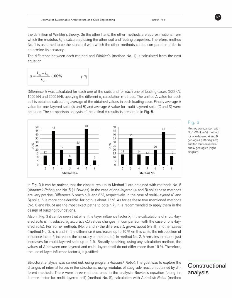
Fig. 3. Method comparison with No.1 (Winkler’s) method for one-layered A and B geologies (left diagram) and for multi-layered C and D geologies (right diagram).

In figure 3 it can be noticed that the closest results to Method 1 are obtained with methods No. 8 (Autodesk Robot) and No. 5 (J. Bowles). In the case of one-layered (A and B) soils these methods are very precise. Difference Δ reach 6 % and 8 %, respectively. In the case of multi-layered (C and D) soils, Δ is more considerable: for both is about 12 %. As far as these two mentioned methods (No. 8 and No. 5) are the most exact paths to obtain ks, it is recommended to apply them in the design of building foundations.

Also in figure 3 it can be seen that when the layer influence factor ki in the calculations of multi-layered soils is introduced, ks accuracy (Δ) values changes (in comparison with the case of one-layered soils). For some methods (No. 5 and 8) the difference Δ grows about 5-8 %. In other cases (method No. 3, 4, 6 and 7), the difference Δ decreases up to 10 % (in this case, the introduction of influence factor ki increases the accuracy of the results). In method No. 2, Δ remains similar: it just increases for multi-layered soils up to 2 %. Broadly speaking, using any calculation method, the values of Δ between one-layered and multi-layered soil do not differ more than 10 %. Therefore, the use of layer influence factor ki is justified.

Constructional analysis

Structural analysis was carried out, using program Autodesk Robot. The goal was to explore the changes of internal forces in the structures, using modulus of subgrade reaction obtained by different methods. There were three methods used in the analysis: Bowles’s equation (using influence

12

45

19

8

25

48

6

05

101520253035404550

2 3 4 5 6 7 8

Δ, %

Method No.

14

35

14 12

20

43

12

05

101520253035404550

2 3 4 5 6 7 8

Δ, %

Method No.

ks,i ks,1

ks,1

100%

Difference Δ was calculated for each one of the soils and for each one of loading cases (500 kN, 1000 kN and 2000 kN), applying the different ks calculation methods. The unified Δ value for each soil is obtained calculating average of the obtained values in each loading case. Finally average Δ value for one-layered soils (A and B) and average Δ value for multi-layered soils (C and D) were obtained. The comparison analysis of these final Δ results is presented in Fig. 5.

Fig. 3 Method comparison with No.1 (Winkler’s) method for one-layered A and B geologies (left diagram) and for multi-layered C and D geologies (right diagram)

the modulus ks is calculated using the other soil and footing properties. Therefore, method No. 1 is assumed to be the standard with which the other methods can be compared in order to determine its accuracy.


(17)

Difference Δ was calculated for each one of the soils and for each one of loading cases (500

kN, 1000 kN and 2000 kN), applying the different ks calculation methods. The unified Δ value for each soil is obtained calculating average of the obtained values in each loading case. Finally average Δ value for one-layered soils (A and B) and average Δ value for multi-layered soils (C and D) were obtained. The comparison analysis of these final Δ results is presented in figure 5.

Fig. 3. Method comparison with No.1 (Winkler’s) method for one-layered A and B geologies (left diagram) and for multi-layered C and D geologies (right diagram).

In figure 3 it can be noticed that the closest results to Method 1 are obtained with methods No. 8 (Autodesk Robot) and No. 5 (J. Bowles). In the case of one-layered (A and B) soils these methods are very precise. Difference Δ reach 6 % and 8 %, respectively. In the case of multi-layered (C and D) soils, Δ is more considerable: for both is about 12 %. As far as these two mentioned methods (No. 8 and No. 5) are the most exact paths to obtain ks, it is recommended to apply them in the design of building foundations.

Also in figure 3 it can be seen that when the layer influence factor ki in the calculations of multi-layered soils is introduced, ks accuracy (Δ) values changes (in comparison with the case of one-layered soils). For some methods (No. 5 and 8) the difference Δ grows about 5-8 %. In other cases (method No. 3, 4, 6 and 7), the difference Δ decreases up to 10 % (in this case, the introduction of influence factor ki increases the accuracy of the results). In method No. 2, Δ remains similar: it just increases for multi-layered soils up to 2 %. Broadly speaking, using any calculation method, the values of Δ between one-layered and multi-layered soil do not differ more than 10 %. Therefore, the use of layer influence factor ki is justified.


Structural analysis was carried out, using program Autodesk Robot. The goal was to explore the changes of internal forces in the structures, using modulus of subgrade reaction obtained by different methods. There were three methods used in the analysis: Bowles’s equation (using influence

12

45

19

8

25

48

6

05

101520253035404550

2 3 4 5 6 7 8

Δ, %

Method No.

14

35

14 12

20

43

12

05

101520253035404550

2 3 4 5 6 7 8

Δ, %

Method No.

ks,i ks,1

ks,1

100%

In Fig. 3 it can be noticed that the closest results to Method 1 are obtained with methods No. 8 (Autodesk Robot) and No. 5 (J. Bowles). In the case of one-layered (A and B) soils these methods are very precise. Difference Δ reach 6 % and 8 %, respectively. In the case of multi-layered (C and D) soils, Δ is more considerable: for both is about 12 %. As far as these two mentioned methods (No. 8 and No. 5) are the most exact paths to obtain ks, it is recommended to apply them in the design of building foundations.

Also in Fig. 3 it can be seen that when the layer influence factor ki in the calculations of multi-lay-ered soils is introduced, ks accuracy (Δ) values changes (in comparison with the case of one-lay-ered soils). For some methods (No. 5 and 8) the difference Δ grows about 5-8 %. In other cases (method No. 3, 4, 6 and 7), the difference Δ decreases up to 10 % (in this case, the introduction of influence factor ki increases the accuracy of the results). In method No. 2, Δ remains similar: it just increases for multi-layered soils up to 2 %. Broadly speaking, using any calculation method, the values of Δ between one-layered and multi-layered soil do not differ more than 10 %. Therefore, the use of layer influence factor ki is justified.

Structural analysis was carried out, using program Autodesk Robot. The goal was to explore the changes of internal forces in the structures, using modulus of subgrade reaction obtained by dif-ferent methods. There were three methods used in the analysis: Bowles’s equation (using in-fluence factor for multi-layered soil) (method No. 5), calculation with Autodesk Robot (method



No. 8) and Winkler’s method (method No. 1). After the analysis, it was noticed that the values of the internal forces obtained from the different three methods were very similar: the differences were up to 1%. As a result, further in this work, only the internal forces obtained using the modu-lus of subgrade reaction calculated by method No. 5 will be shown.

Calculation scheme is represented in Fig. 4. The modelled structure is a two-storied building. The height of the first storey is 3 m. The distance between the floor of the first storey and the bottom chord of the truss is 3 m. The first floor has five 6 meters long spans. The span of the second floor is 30 m. In the calculations, the transverse frame is being analysed. Its step in the longitudinal direction of the building is 6 meters.

Fig. 4 Calculation scheme

factor for multi-layered soil) (method No. 5), calculation with Autodesk Robot (method No. 8) and Winkler’s method (method No. 1). After the analysis, it was noticed that the values of the internal forces obtained from the different three methods were very similar: the differences were up to 1%. As a result, further in this work, only the internal forces obtained using the modulus of subgrade reaction calculated by method No. 5 will be shown.

Calculation scheme is represented in fig. 4. The modelled structure is a two-storied building. The height of the first storey is 3 m. The distance between the floor of the first storey and the bottom chord of the truss is 3 m. The first floor has five 6 meters long spans. The span of the second floor is 30 m. In the calculations, the transverse frame is being analysed. Its step in the longitudinal direction of the building is 6 meters.

Fig. 4. Calculation scheme

The redistribution of internal forces was explored in the transverse frame of the structure.

Three different geological situations were assumed in order to carry out the analysis: a) Situation No. 1: absolutely rigid soil under all the supports of the building. b) Situation No. 2: relatively weak soil (soil E) under all the supports of the building. c) Situation No. 3: relatively strong soil (soil F) under supports S1 and S2; relatively weak soil

(soil E) under supports S3, S4, S5 and S6. Now the soil was chosen to be different from the soil used in the previous chapter. The soil in

this chapter was chosen with the purpose to give potentially extreme differences of internal forces. The elastic behaviour of the soil is modelled introducing springs in the situations No. 2 and

No. 3. The elastic modulus of those springs is the modulus of subgrade reaction of the considered soils E and F.

The properties of soils E and F are shown in Table 2. Those characteristics have been obtained by evaluating geological boreholes from the same construction site. In spite of their proximity, their characteristics are considerably different. Table 2. Characteristics of layers of soils E and F

Layer No. Soil Hsl, m qc, MPa E0, MPa c', kPa φ, ̊ γ, kN/m3 ν Soil E

1 Sand 2,1 3,0 9 - 32 21,0 0,25 2 Coarse sand 1,2 6,0 18 - 33 18,0 0,2 3 Coarse sand 1,1 3,0 9 - 33 17,5 0,2 4 Coarse sand 0,8 11,0 33 1,0 37 21,0 0,2 5 Sandy silty clay 1,2 6,0 60 70,0 26 23,0 0,3

Soil F 3 Sand with some gravel 1,1 11 37 1 37 19,5 0,25 4 Sand with some gravel 1,6 9 36 1 36 19,0 0,25

The redistribution of internal forces was explored in the transverse frame of the structure. Three different geological situations were assumed in order to carry out the analysis:

a) Situation No. 1: absolutely rigid soil under all the supports of the building.

b) Situation No. 2: relatively weak soil (soil E) under all the supports of the building.

c) Situation No. 3: relatively strong soil (soil F) under supports S1 and S2; relatively weak soil (soil E) under supports S3, S4, S5 and S6.

Now the soil was chosen to be different from the soil used in the previous chapter. The soil in this chapter was chosen with the purpose to give potentially extreme differences of internal forces.

The elastic behaviour of the soil is modelled introducing springs in the situations No. 2 and No. 3. The elastic modulus of those springs is the modulus of subgrade reaction of the considered soils E and F.

The properties of soils E and F are shown in Table 2. Those characteristics have been obtained by evaluating geological boreholes from the same construction site. In spite of their proximity, their characteristics are considerably different.

The bending moment diagrams under the three different described situations are shown in Fig. 5.

Note: boxes of internal forces of columns have solid lines. Boxes of internal forces of beams have dashed lines. Values of bending moments in Fig. 5 are divided by 527,67 in beams and by 161,7 in columns (maximum values).

In Fig. 5, it can be noticed that, when the springs are introduced (situation No. 2) instead of rigid supports (situation 1), bending moments in the beams increase up to 43 %. The maximum in-crease of bending moments can be noticed in beams B1 and B5, in the places, where those beams are connected to columns C1 and C6 respectively. However, the values of bending moments in several beams decrease. The biggest decline of bending moments is noticed in the places, where beams are connected to columns C2 and C5. In these places the values of bending moments de-


Table 2Characteristics of layers of soils E and F

Layer No. Soil Hsl, m qc, MPa E0, MPa c’, kPa φ, ° γ, kN/m3 ν

Soil E

1 Sand 2,1 3,0 9 - 32 21,0 0,25

2 Coarse sand 1,2 6,0 18 - 33 18,0 0,2

3 Coarse sand 1,1 3,0 9 - 33 17,5 0,2

4 Coarse sand 0,8 11,0 33 1,0 37 21,0 0,2

5 Sandy silty clay 1,2 6,0 60 70,0 26 23,0 0,3

Soil F

3 Sand with some gravel 1,1 11 37 1 37 19,5 0,25

4 Sand with some gravel 1,6 9 36 1 36 19,0 0,25

5 Coarse sand 2,0 4 12 - 33 17,5 0,2

6 Coarse sand 0,5 12 36 1 38 21,0 0,2

7 Sandy silty clay 1,5 5 50 70 26 23,0 0,3


Fig. 5Diagrams of bending moments

Table 3 Legend of the diagrams

5 Coarse sand 2,0 4 12 - 33 17,5 0,2 6 Coarse sand 0,5 12 36 1 38 21,0 0,2 7 Sandy silty clay 1,5 5 50 70 26 23,0 0,3


The bending moment diagrams under the three different described situations are shown in Fig.

5. Note: boxes of internal forces of columns have solid lines. Boxes of internal forces of beams have dashed lines. Values of bending moments in Fig. 5 are divided by 527,67 in beams and by 161,7 in columns (maximum values).

Fig. 5. Diagrams of bending moments

Table 3. Legend of the diagrams

Case Marking Note

1. Situation No. 1 2. Situation No. 2 3. Situation No. 3

In figure 5, it can be noticed that, when the springs are introduced (situation No. 2) instead of rigid supports (situation 1), bending moments in the beams increase up to 43 %. The maximum increase of bending moments can be noticed in beams B1 and B5, in the places, where those beams are connected to columns C1 and C6 respectively. However, the values of bending moments in several beams decrease. The biggest decline of bending moments is noticed in the places, where beams are connected to columns C2 and C5. In these places the values of bending moments decreased by up to 21 %. There are also significant differences of bending moments in the columns. Bending moments increased by up to 41 % at the top of the columns C1 and C6.

Introducing different types of soil (situation No. 3) and comparing it to the results obtained from situation No. 2, where there is only one type of soil, changes are also noticeable. The maximum increase of bending moments, 72 %, can be noticed in beam B1, in the place where this beam is connected to column C2. Comparing the latter situations, there is a considerable decrease of bending moments in some structures. For example, the bending moment in the midspan of beam B1 was up to 21 %. Although the changes of bending moments in columns are not so significant, they should also be evaluated. The most noticeable decrease, 23 % occurred at the top of column C1. The increase of bending moments in columns is not considerable.

Diagrams of axial forces under three types of soil rigidity situations are represented in Fig. 6 Those situations are represented in Table 3. Note: Values of axial forces in Fig. 6 are divided by the value of maximum axial force - 782,76.

Case Marking Note

1. Situation No. 1

2. Situation No. 2

3. Situation No. 3

creased by up to 21 %. There are also signif-icant differences of bending moments in the columns. Bending moments increased by up to 41 % at the top of the columns C1 and C6.

Introducing different types of soil (situation No. 3) and comparing it to the results ob-tained from situation No. 2, where there is only one type of soil, changes are also noticeable. The maximum increase of bending moments, 72 %, can be noticed in beam B1, in the place where this beam is connected to column C2. Com-paring the latter situations, there is a considerable decrease of bending moments in some struc-tures. For example, the bending moment in the midspan of beam B1 was up to 21 %. Although the changes of bending moments in columns are not so significant, they should also be evaluated. The most noticeable decrease, 23 % occurred at the top of column C1. The increase of bending moments in columns is not considerable.


Diagrams of axial forces under three types of soil rigidity situations are represented in Fig. 6 Those situations are represented in Table 3.

Note: Values of axial forces in Fig. 6 are divided by the value of maximum axial force - 782,76.

Fig. 6 Diagrams of axial forces

Fig. 6. Diagrams of axial forces

Maximum and minimum axial forces in columns were obtained. However, under all of those

situations tension did not occur and the differences of axial forces are very low. As a consequence, maximum axial forces are more relevant and only the changes of maximum axial forces will be discussed.

In the column C1 there are no large differences of axial forces under the three situations of soil rigidity. In this column there is no difference between the results obtained from situations No. 2 and No. 1. There are significant changes under the situation No. 3, when axial force decreases by 5 %. In the column C2 the changes of axial forces under situation No. 2 decrease 6 % in comparison to situation No. 1. Under the situation No. 3, axial force increases by up to 10 %. Axial forces in column C3 under situations No. 1 and No. 2 are similar. However, in the situation No. 3 the axial forces of this column decrease by 15 %. There are no considerable changes of the axial forces in columns C4 and C6. Axial forces in column C5 only diverge under the situation No. 1. Under the elastic situations (No. 2 and 3) the values of axial forces decreased by 6 % in comparison to situation No. 1.

Diagrams of lateral forces under three types of soil rigidity cases are represented in Fig. 7. Those cases are represented in Table 3. Note: Values of lateral forces in Fig. 7 are divided by 382,63 in beams and by 73,5 in columns (maximum values).

Fig. 7. Diagrams of shear forces

When the springs are introduced (situation No. 2) instead of rigid supports (situation No. 1),

the lateral forces in the beams increase by up to 7 %. This maximum increase is noticed in beams B1

Maximum and minimum axial forces in columns were obtained. However, under all of those sit-uations tension did not occur and the differences of axial forces are very low. As a consequence, maximum axial forces are more relevant and only the changes of maximum axial forces will be discussed.

In the column C1 there are no large differences of axial forces under the three situations of soil rigidity. In this column there is no difference between the results obtained from situations No. 2 and No. 1. There are significant changes under the situation No. 3, when axial force decreases by 5 %. In the column C2 the changes of axial forces under situation No. 2 decrease 6 % in comparison to situation No. 1. Under the situation No. 3, axial force increases by up to 10 %. Axial forces in column C3 under situations No. 1 and No. 2 are similar. However, in the situation No. 3 the axial forces of this column decrease by 15 %. There are no considerable changes of the axial forces in columns C4 and C6. Axial forces in column C5 only diverge under the situation No. 1. Under the elastic situations (No. 2 and 3) the values of axial forces decreased by 6 % in comparison to situ-ation No. 1.

Diagrams of lateral forces under three types of soil rigidity cases are represented in Fig. 7. Those cases are represented in Table 3.

Note: Values of lateral forces in Fig. 7 are divided by 382,63 in beams and by 73,5 in columns (maximum values).

Fig. 7 Diagrams of shear forces

Fig. 6. Diagrams of axial forces

Maximum and minimum axial forces in columns were obtained. However, under all of those

situations tension did not occur and the differences of axial forces are very low. As a consequence, maximum axial forces are more relevant and only the changes of maximum axial forces will be discussed.

In the column C1 there are no large differences of axial forces under the three situations of soil rigidity. In this column there is no difference between the results obtained from situations No. 2 and No. 1. There are significant changes under the situation No. 3, when axial force decreases by 5 %. In the column C2 the changes of axial forces under situation No. 2 decrease 6 % in comparison to situation No. 1. Under the situation No. 3, axial force increases by up to 10 %. Axial forces in column C3 under situations No. 1 and No. 2 are similar. However, in the situation No. 3 the axial forces of this column decrease by 15 %. There are no considerable changes of the axial forces in columns C4 and C6. Axial forces in column C5 only diverge under the situation No. 1. Under the elastic situations (No. 2 and 3) the values of axial forces decreased by 6 % in comparison to situation No. 1.

Diagrams of lateral forces under three types of soil rigidity cases are represented in Fig. 7. Those cases are represented in Table 3. Note: Values of lateral forces in Fig. 7 are divided by 382,63 in beams and by 73,5 in columns (maximum values).

Fig. 7. Diagrams of shear forces

When the springs are introduced (situation No. 2) instead of rigid supports (situation No. 1),

the lateral forces in the beams increase by up to 7 %. This maximum increase is noticed in beams B1


When the springs are introduced (situation No. 2) instead of rigid supports (situation No. 1), the lat-eral forces in the beams increase by up to 7 %. This maximum increase is noticed in beams B1 and B5, in the connections to columns C1 and C6. The decrease of lateral forces in some of the beams is also considerable. Maximum decrease is noticed in beam B2, in the connection to column C2. This maximum decrease reaches 6 %. When comparing situation No. 2 to situation No. 1, it can be seen, that lateral forces increase in all of the columns of the first floor (columns C1 to C6). The maximum increase, up to 38 %, occurs in columns C1 and C6.

Comparing the values of the lateral forces obtained from situation No. 3 to the results obtained from situation No. 3, significant changes can be noticed. The maximum increase of lateral forces occurs in beam B2, in its connection to column C2. The values obtained in situation No. 3 are 21 % larger than in situation No. 2. The maximum decrease is also in beam B2. This decrease is noted at the place where the beam B2 is connected to the column C3. The values obtained in situation No. 3 decrease 18 % in comparison to situation No. 2. While comparing the changes of lateral forces in columns under situation No. 3 to situation No. 2, the maximum increase, up to 28 %, can be noticed in columns C4 and C5. The maximum decrease also occurs in the same columns. It is possible because there are many load combinations. This leads to the fact that there are diagrams on both sides of the columns. Lateral forces increase on one side and decrease on the other side.

1 The comparable analysis of calculation methods of the modulus of subgrade reaction was performed. When analysing it was assumed that the most realistic results are obtained

with the first method (Winkler’s). The accuracy of other methods was determined by compar-ing those methods with the method No. 1 in calculating the difference Δ. The closest results to first method were derived from calculation methods No. 5 (Bowles) and No. 8 (Autodesk Robot) where the difference Δ does not exceed 12 %. Applying methods No. 2, 4 and 6 the value difference Δ oscillate vary from 12 % to 25 %. The largest difference from the first method is obtained calculating by methods No. 3 (simplified Vesic’s equation) and No. 7 (Selvadurai) when the difference Δ reaches 48 %.

2 Most of the considered methods are dedicated to homogenous soils. However, in practise often occurs that the soil is consisted of many layers, which have different properties. In

order to calculate the modulus of subgrade reaction of such soil, it is proposed to use the layer influence factor ki. By some methods (method No. 5 and 8) the difference of methods increased in one-layer case by 5 %. The difference Δ of other methods remained similar or even less than Δ of these methods in one-layer case. The differences Δ, while calculating the coefficient ks by the same method for one-layered and multi-layered soil, never differed more than 10 %. Therefore, the application of the coefficient ki is advisable and rational in the determination of the modulus of subgrade reaction of a multi-layered soil.

3 When the analysis of considered building was performed, it was determined that eval-uation of the modulus of subgrade reaction has considerable influence for the internal

forces of the structures. Redistribution of internal forces occurred with particular intensity when there were modelled different base ground stiffness (situation No. 3) under supports S1 and S2. Redistribution of bending moments was the most relevant: under situation No. 3 it increased more than 70 %. Moreover, there was a considerable variation of shear forces in the columns. Evaluating the base ground stiffness (situation No. 2) and comparing it with the internal forces of the case where the supports are rigid (situation No. 1), the increase reached even 40 %. In beams considerable changes of shear forces were determined introducing the different types of soil (situation No. 3). It exceeded 20 %. The changes of axial forces were not such considerable (up to 10 %). However, the evaluation of those changes is essential.

4 The analysis of structures was performed evaluating the different modulus of subgrade reaction in several cases: Bowles’s method (No. 5), Winkler’s method (No. 1) and Autodesk

Robot method (No. 8). Obtained internal forces were compared in all cases. Calculating the stiff-

Conclusions


ness with method No. 5 (using the influence factor for multi-layered soil ki) and comparing it with the other chosen methods, inconsiderable differences were obtained (up to 1 %). As a con-sequence, it is obvious that results obtained from method No. 5 are accurate, and that influence factor ki is reliable and appropriate to use in the analysis of multi-layered soils.

EN 1997-2 (2007) (English): Eurocode 7: Geotechni-cal design - Part 2: Ground investigation and testing.

Bowles, J. E. Foundation Analysis and Design. 5th ed. New York: Mc Graw-Hill; 1997.

Bjerrum L. Contribution to the discussion. Sect. 6, 6th E.C.S.M.F.E., 1963; Wiesbaden; vol. 2: 135-137.

Gorbunov-Posadov M.I., Malikova T. A., Solomin V. I. Calculation of structures of elastic bed. Moscow: Stroyizdat; 1984.

Polshin D. E., Tokar R. A. Maximum allow-able non-uniform settlement of structures. 4th I.C.S.M.F.E., 1957; London; Vol. 1: 402-405.

Rowe, R. K. Geotechnical and Geoenvironmental Engineering Handbook. 1st ed., New York, Springer science + Bussiness Media, 2001.

Sadrekarimi, J. Comparative study of methods of determination of coefficient of subgrade reaction. Electronic Journal of Geotechnical Engineering, 2009, Vol. 14, Bund. E.

Schleicher, F. Zur theorie des baugrundes [The theory of soils]. Bauingenieur, 1926; 7: 931–935, 949–952.

Selvadurai, A.P.S. The flexure of an infinite strip of finite width embedded in an isotropic elastic medium of finite extent. Int. J. Numer. Anal. Meth. Geomech., 1984; 8: 157-166.

Skempton A. W., McDonalds D. H. Allowable settle-ments of buildings. Proc. I.C.E, 1956; London; Vol 5: 727-768.

Šližytė, D., Medzvieckas, J., Mackevičius, R. Pamatai ir pagrindai [Foundations and grounds]. Vilnius: Technika; 2012.

Vesic, A. B.Beams on Elastic Subgrade and the Win-kler’s Hypothesis. Proceedings of 5th International Conference of Soil Mechanics, 1961; Paris: 845-850.

Terzaghi, K. V. Evaluation of Coefficient of Subgrade Reaction, Geotechnique,1955; 5(4): 297-326.

Ziaie-Moayed, R., Janbaz, M. Effective Parameters on Modulus of subgrade Reaction in Clayey Soils”. Journal of Applied Sciences, 2009; 9 (22): 4006-4012.

Zhemochkin B. N., Sinitsyn A. P. Practical meth-ods of calculation for beams and slabs on elastic foundation without usig the Winkler hypothesis. Moscow: Gosstroyizdat; 1947.

IGNACIO VILLALON FORNESMaster’s degree studentKaunas University of Technology, Department of Building Structures.

Main research area

Calculation and analysis of building structures

AdressStudentu st. 48, LT-51367, Kaunas, LithuaniaTel.: +370 675 79085E-mail: [email protected]

References

DEIVIDAS MARTINAVIČIUSMaster’s degree student

Kaunas University of Technology, Department of Building Structures.

Main research area



MINDAUGAS GRICIUSMaster’s degree student

Kaunas University of Technology, Department of Building Structures.

Main research area



ŠARŪNAS KELPŠALecturer

Kaunas University of Technology, Department of Building Structures

Main research area

Reinforced concrete. Structural analysis.

Address

Studentu st. 48, LT-51367, Kaunas, LithuaniaTel.: +370 37 30 04 73E-mail: [email protected]

MINDAUGAS KASIULEVIČIUS

Director

JSC “Smailusis skliautas”

Main research area

Timber structures. Structural analysis

Adress

Piliakalnio st. 3, LT-46224 Kaunas, LithuaniaTel.: +370 37 33 04 40E-mail: mindaugas kasiulevicius@ yachoo.com

About the authors

evaluation of base ground - sace.ktu.lt

Documents