evaluation of archived and off-line diagnosed vertical ... · 40 project (i and iii). the archived...
TRANSCRIPT
Atmos Chem Phys 4 2313ndash2336 2004wwwatmos-chem-physorgacp42313SRef-ID 1680-7324acp2004-4-2313European Geosciences Union
AtmosphericChemistry
and Physics
Evaluation of archived and off-line diagnosed vertical diffusioncoefficients from ERA-40 with 222Rn simulations
D J L Olivi e12 P F J van Velthoven1 and A C M Beljaars3
1Royal Netherlands Meteorological Institute De Bilt The Netherlands2Eindhoven University of Technology Eindhoven The Netherlands3European Centre for Medium-range Weather Forecasts Reading UK
Received 15 June 2004 ndash Published in Atmos Chem Phys Discuss 3 August 2004Revised 2 November 2004 ndash Accepted 11 November 2004 ndash Published 26 November 2004
Abstract Boundary layer turbulence has a profound influ-ence on the distribution of tracers with sources or sinks at thesurface The 40-year ERA-40 meteorological data set of theEuropean Centre for Medium-range Weather Forecasts con-tains archived vertical diffusion coefficients We evaluatedthe use of these archived diffusion coefficients versus off-linediagnosed coefficients based on other meteorological param-eters archived during ERA-40 by examining the influence onthe distribution of the radionuclide222Rn in the chemistrytransport model TM3 In total four different sets of verti-cal diffusion coefficients are compared (i) 3-hourly verticaldiffusion coefficients archived during the ERA-40 project(ii) 3-hourly off-line diagnosed coefficients from a non-localscheme based onHoltslag and Boville(1993) Vogelezangand Holtslag(1996) andBeljaars and Viterbo(1999) (iii) 6-hourly coefficients archived during the ERA-40 project and(iv) 6-hourly off-line diagnosed coefficients based on a localscheme described inLouis (1979) and Louis et al(1982)The diffusion scheme to diagnose the coefficients off-line in(ii) is similar to the diffusion scheme used during the ERA-40 project (i and iii)
The archived diffusion coefficients from the ERA-40project which are time-averaged cause stronger mixing thanthe instantaneous off-line diagnosed diffusion coefficientsThis can be partially attributed to the effect of instantaneousversus time-averaged coefficients as well as to differencesin the diffusion schemes The 3-hourly off-line diagnosis ofdiffusion coefficients can reproduce quite well the 3-hourlyarchived diffusion coefficients
Atmospheric boundary layer heights of the sets (ii) and(iii) are also compared Both were found to be in reason-able agreement with observations of the atmospheric bound-ary layer height in Cabauw (the Netherlands) and from theFIFE-campaign (United States) during summer
Correspondence toD J L Olivie(olivieknminl)
Simulations of222Rn with the TM3 model using these foursets of vertical diffusion coefficients are compared to surfacemeasurements of222Rn at the mid-latitude continental sta-tions Freiburg Schauinsland Cincinnati and Socorro in or-der to evaluate the effect of these different sets of diffusioncoefficients on the tracer transport It is found that the dailycycle of the222Rn concentration is well represented using3-hourly diffusion coefficients Comparison with observa-tions of222Rn data with the station in Schauinsland which issituated on a hill shows that all considered schemes underes-timate the amplitude of the daily cycle of the222Rn concen-tration in the upper part of the atmospheric boundary layer
1 Introduction
Boundary layer turbulence is an important transport mecha-nism in the troposphere (Wang et al 1999) In the convec-tive or turbulent atmospheric boundary layer (ABL) tracerscan be transported throughout the height range of the ABLin time intervals of tens of minutes All species emitted atthe surface must pass through the ABL in order to reach thefree troposphere Because turbulence acts on spatial scalesthat are much smaller than the typical size of the grid cells ofglobal atmospheric models turbulent diffusion must be pa-rameterised in these models
The European Centre for Medium-range Weather Fore-casts (ECMWF) re-analysis project (ERA-40) aims at pro-viding a consistent time series of the state of the global at-mosphere for the period 1957ndash2002 (Simmons and Gibson2000) A wide variety of meteorological fields were archivedin ERA-40 In the earlier ERA-15 re-analysis project (Gib-son et al 1997) where the atmosphere for the period 1979ndash1993 has been reanalysed meteorological fields describingsmall-scale transport like convection or boundary layer tur-bulence were not archived The more recent ERA-40 data setis one of the first long-term meteorological data sets where
copy 2004 Author(s) This work is licensed under a Creative Commons License
2314 D J L Olivie et al Vertical diffusion coefficients from ERA-40
vertical diffusion coefficients for heat are archived (availableas 3- or 6-hourly averaged values)
Meteorological data sets such as ERA-40 and ERA-15 arecommonly used to study the transport and chemical evolu-tion of atmospheric gases and aerosols in chemical transportmodels (CTMs) The chemical transport model TM3 (TracerModel Version 3) is a global atmospheric model which is ap-plied to evaluate the atmospheric composition and changesherein caused by natural and anthropogenic changes For de-scribing the turbulent transport it can use different turbu-lent diffusion data Until now two off-line vertical diffu-sion schemes have been used in the TM3 model where thediffusion coefficients are diagnosed off-line based on otherregularly (eg 6-hourly) archived meteorological fields Thefirst scheme based onLouis (1979) andLouis et al(1982)is a local diffusion scheme that describes the vertical diffu-sion coefficient as a function of a mixing length scale thelocal gradient of the wind and the virtual temperature How-ever under convective conditions when the largest trans-porting eddies may have sizes similar to the depth of theABL local schemes do not perform well (Troen and Mahrt1986) the characteristics of the large eddies are not properlytaken into account The second scheme based on a combi-nation ofHoltslag and Boville(1993) Vogelezang and Holt-slag(1996) andBeljaars and Viterbo(1999) is a non-localdiffusion scheme Non-local ABL schemes often contain aterm that describes counter gradient transport by the largeeddies (Troen and Mahrt 1986) and prescribe the shape ofthe vertical profile of the diffusion coefficient Apart fromthe meteorological fields needed for a local scheme a non-local scheme also uses the surface sensible and latent heatfluxes The vertical exchange has been shown to be morepronounced with non-local schemes than with local schemes(Holtslag and Boville 1993 Holtslag et al 1995) The3-hourly off-line scheme (Holtslag and Boville 1993 Vo-gelezang and Holtslag 1996 Beljaars and Viterbo 1999) iscurrently most used in the TM3 model The 6-hourly off-linescheme (Louis 1979 Louis et al 1982) was until recentlyused in the TM3 model for various studiesDentener et al(2003) used meteorological data from the ERA-15 project(which does not provide 3-hourly surface latent heat fluxes)and the 6-hourly off-line scheme (Louis 1979 Louis et al1982) From now on however the ERA-40 data set allowsthe use of archived vertical diffusion data (3-hourly or 6-hourly) in the TM3 model One of the first to use archivedsub-grid meteorological parameters wasAllen et al (1996)They used archived convective mass fluxes and detrainmentsas well as the ABL heights An advantage of the use ofarchived meteorological fields to describe small-scale trans-port in CTMs is the consistency of these fields with thearchived fields of cloud cover temperature humidity or pre-cipitation
The effect on the transport of tracers by the diffusion datacan be studied by making222Rn simulations with CTMs222Rn is an excellent tracer to study the transport character-
istics on short time scales (hours to weeks) because it hasan almost uniform emission rate over land and is only lostthrough radioactive decay with an e-folding lifetime of about55 days (Dentener et al 1999 Balkanski and Jacob 1990Kritz et al 1990 Brost and Chatfield 1989 Polian et al1986) Therefore222Rn has been used extensively to evaluateparameterisations of convective transport (Mahowald et al1997 Allen et al 1996 Feichter and Crutzen 1990 Jacoband Prather 1990) and ABL diffusion (Stockwell and Chip-perfield 1999 Stockwell et al 1998 Jacob et al 1997 Leeand Larsen 1997 Mahowald et al 1997) in atmosphericmodels
In this work we try to answer the following questions(1) How well is the mid-latitude summer time ABL height re-produced in the ERA-40 data and in an off-line model drivenby ERA-40 data (2a) Can diffusion coefficients be repro-duced accurately off-line for use in CTMs (2b) How dolocal ABL schemes perform versus non-local ABL schemeswhen applied off-line (3a) How crucial is a 3-hourly timeresolution for diffusion data for CTM-modelling (3b) Whatis the influence of using time-averaged diffusion coefficientson the tracer transport in CTMs
To answer these questions we will start with a descriptionof the TM3 model and the diffusion schemes that generatethe different sets of vertical diffusion coefficients (Sect 2)In that section we will also describe the222Rn emission sce-nario in the TM3 model the222Rn observations and theABL height observations In Sect 3 we will first comparethe vertical diffusion coefficients from the different schemesThen we will compare the modelled ABL height at two mid-latitude stations with observations Next we will compare the222Rn concentration which is modelled in the TM3 modelusing the different sets of diffusion data with surface mea-surements of the222Rn concentration at four selected surfacestations In Sect 4 we will formulate the conclusions andformulate some recommendations
2 Methods
21 The TM3 chemistry transport model
The chemical transport model TM3 (Tracer Model Version3) is a global atmospheric CTM with a regular longitude-latitude grid and hybridσ -pressure levels (Lelieveld andDentener 2000 Houweling et al 1998 Heimann 1995)The meteorological input data for TM3 from ERA-40 isavailable for 1957 to 2002 For dynamics calculationsERA-40 used a spectral truncation of T159 The physi-cal calculations were done on a reduced Gaussian grid of160 nodes (N80) In the vertical 60 hybridσ -pressure lev-els (Simmons and Burridge 1981) were used reaching upto 01 hPa To be used in the TM3 model the meteorologi-cal data is interpolated or averaged to the desired TM3 gridcells (Bregman et al 2003) For advection of the tracers
Atmos Chem Phys 4 2313ndash2336 2004 wwwatmos-chem-physorgacp42313
D J L Olivie et al Vertical diffusion coefficients from ERA-40 2315
the model uses the slopes scheme developed by Russel andLerner (Russell and Lerner 1981) To describe the effect ofconvective transport on the tracer concentration we used thearchived convective mass fluxes from the ERA-40 data set(Olivi e et al 2004) The convection scheme in the ECMWF-model used during the ERA-40 project is based onTiedtke(1989) Gregory et al(2000) andNordeng(1994)
The vertical diffusion of tracers in the TM3 model is de-scribed with a first order closure scheme The net turbulenttracer fluxwprimeχ prime is expressed as
minus wprimeχ prime = Kz
partχ
partz (1)
whereKz is the vertical diffusion coefficient for heatw thevertical velocityχ the tracer concentration andz the heightabove the surface It is assumed that the vertical diffusioncoefficient for tracers is equal to the vertical diffusion coeffi-cient for heat In contrast toHoltslag and Boville(1993) andWang et al(1999) there is no counter gradient term in theTM3 implementation
The vertical diffusion coefficients are applied in the TM3model by converting the vertical diffusion coefficients intoupward and downward vertical air mass fluxes of equal mag-nitude which model the exchange between two model layersThese air mass fluxes are combined with the vertical con-vective mass fluxes from the convection parameterisation tocalculate the sub-grid scale vertical tracer transport with animplicit numerical scheme This allows the time steps in theTM3 model to be rather large without introducing stabilityproblems In the case of very large time steps the effect ofthe scheme is that it pushes the tracer concentration at onceto its equilibrium distribution In this study we used a timestep of 1 h for the small-scale vertical transport
From Eq (1) one derives that the dimensions ofKz areL2Tminus1 Taking the ABL height as a representative lengthscale for the effect of diffusion gives a relationship betweenKz and the time scale of turbulent diffusion If for examplethe ABL height is 1000 m andKz is 300 m2s one finds atime scale of around 1 h This means that a tracer initiallyonly present at the surface will be well mixed throughoutthe complete ABL on a time scale of 1 h
22 Vertical diffusion data
Different sets of vertical diffusion coefficients are used in theTM3 model We will briefly describe the schemes that areused to calculate these data sets
221 The ERA-40 3-hourly and 6-hourly diffusion coeffi-cients
The scheme as it is used in the ERA-40 project is describedin the documentation of the cycle CY23r4 of the ECMWFmodel see httpwwwecmwfintresearchifsdocsCY23r4It is a non-local scheme The coefficients for vertical dif-
fusion of heat were stored during the ERA-40 project as 3-hourly averaged values They can also be combined to 6-hourly averaged values
Different formulations are used based on the stabilityregime that is determined by the virtual potential temperatureflux (wprimeθ prime
v)0 If the surface layer is unstable ((wprimeθ primev)0gt0)
then a method according toTroen and Mahrt(1986) is ap-plied This method determines the ABL heighth using aparcel method where the parcel is lifted from the minimumvirtual temperature rather than from the surface The dimen-sionless coefficient for the excess of the parcel temperatureis reduced from 65 (Troen and Mahrt 1986) or 85 (Holt-slag and Boville 1993) to 2 (to get a well controlled entrain-ment rate and a less aggressive erosion of inversions) In theABL the vertical profile of diffusion coefficients is prede-fined (Troen and Mahrt 1986)
Kz = κ wh z(1 minus
z
h
)2 (2)
where wh is a turbulent velocity scale andκ=04 theVon Karman constant At the top of the ABL there is an ex-plicit entrainment formulation in the capping inversion Thevirtual heat flux at the top of the ABL is taken proportionalto the surface virtual heat flux
(wprimeθ primev)h = minusC (wprimeθ prime
v)0 (3)
with C=02 andθv the virtual potential temperature Know-ing the flux the diffusion coefficient at the top of the ABLcan be expressed as
Kz = C(wprimeθ prime
v)0partθv
partz
(4)
wherepartθv
partzis the virtual potential temperature gradient in the
inversion layerIf the surface layer is stable ((wprimeθ prime
v)0lt0) the diffusion co-efficients are determined by the gradient Richardson numberRi which is defined as
Ri =g
θ
partθpartz∣∣∣ partvpartz
∣∣∣2 (5)
wherev is the horizontal wind velocity When the atmo-sphere is locally unstable (Rilt0) then
Kz =l2h
8m 8h
∣∣∣∣partv
partz
∣∣∣∣ (6)
where
8m(ζ ) = (1 minus 16ζ )minus14 (7)
and where
8h(ζ ) = (1 minus 16ζ )minus12 (8)
wwwatmos-chem-physorgacp42313 Atmos Chem Phys 4 2313ndash2336 2004
2316 D J L Olivie et al Vertical diffusion coefficients from ERA-40
whereζ is taken equal toRi The mixing lengthlh is calcu-lated according to
1
lh=
1
κ z+
1
λh
(9)
The asymptotic mixing lengthλh [m] is defined as
λh = 30+120
1 +(
z4000
)2 (10)
wherez [m] is the height above the surface The asymptoticmixing lengthλh is a typical length scale in a neutral atmo-sphere for the vertical exchange of some quantity (momen-tum heat or tracer) due to turbulent eddies In the lowestlayers of the atmosphere the size of the turbulent eddies islimited by the presence of the earthrsquos surface which is takeninto account in the mixing lengthlh in Eq (9)
When the atmosphere is locally stable (Rigt0) ζ is readfrom a table (ζ=ζ(Ri)) The diffusion coefficients are cal-culated with
Kz = l2h
∣∣∣∣partv
partz
∣∣∣∣ Fh(Ri) (11)
where the stability functionFh(Ri) is a revised function oftheLouis et al(1982) function (Beljaars and Viterbo 1999)
Fh(Ri) =1
1 + 2b Riradic
1 + d Ri (12)
whereb=5 andd=1 This formulation has less discrepancybetween momentum and heat diffusion the ratio of momen-tum and heat diffusion is reduced (Viterbo et al 1999) Theformulation ofKz in case of a stable surface layer also ap-plies to the formulation ofKz above the ABL in case of anunstable surface layer
The calculation of the atmospheric boundary layer heightstored during the ERA-40 project is also described in the in-formation about the cycle CY23r4 As well in the stablein the neutral as in the unstable case a parcel lifting methodproposed byTroen and Mahrt(1986) is used They use a crit-ical bulk Richardson numberRib=025 The bulk Richard-son number is based on the difference between quantities atthe level of interest and the lowest model level This ABLheight is available every 3 h and represents an instantaneousvalue We only studied the 6-hourly values We will referto these 3-hourly diffusion coefficients as E3 and to these6-hourly diffusion coefficients and 6-hourly ABL heights asE6
222 The TM3 off-line 3-hourly and 6-hourly diffusion co-efficients
The first set of off-line diagnosed diffusion coefficients inTM3 is calculated with a scheme that is rather similar tothe above-described scheme It is a non-local scheme basedon Holtslag and Boville(1993) Vogelezang and Holtslag
(1996) andBeljaars and Viterbo(1999) The diffusion co-efficients are calculated every 3 h based on 3-hourly latentand sensible heat fluxes and 6-hourly fields of wind tem-perature and humidity It has been implemented and testedin the TM3 model (Jeuken 2000 Jeuken et al 2001) ThecalculatedKz values are instantaneous values
Although the scheme is rather similar to the aforemen-tioned E3E6 scheme there are some differences (i) a bulkRichardson criterion instead of a parcel ascent method isused to determine the height of the ABL (ii) there is no en-trainment formulation at the top of the ABL (iii) the temper-ature excess of the large eddies under convective conditionsis larger (iv) the prescribed profile of the asymptotic mixinglength is different and (v) the stability functions are differ-ent
If the surface layer is unstable ((wprimeθ primev)0gt0) a prescribed
profile of the vertical diffusion coefficients as in Eq (2) isused According toVogelezang and Holtslag(1996) the ABLheighth is the layer where the bulk Richardson number
Rib =
gθvs
(θvh minus θvs)(h minus zs)
|vh minus vs |2 + b u2
lowast
(13)
reaches a critical valueRib=03 (in Vogelezang and Holtslag(1996) the critical value isRib=025) The indexs refers tovalues in the lowest model layer the indexh refers to valuesat the top of the ABLulowast is the friction velocity The valuefor b=100 The exact ABL height is calculated by linearinterpolation The temperature excess under convective con-ditions is calculated using a coefficient with value 85 (versus2 in the E3E6 case)
If the surface layer is stable ((wprimeθ primev)0lt0) the diffusion co-
efficients are calculated with Eq (11) When the atmosphereis locally stable (Rigt0) we take
Fh(Ri) =1
1 + 10Riradic
1 + Ri (14)
while when the atmosphere is locally unstable (Rigt0) wetake
F(Ri) = 1 (15)
Above the ABL a formulation according to theLouis(1979) scheme is used In the free atmosphere the stabil-ity functions in the unstable case (Rilt0) (Williamson et al1987 Holtslag and Boville 1993) is
Fh(Ri) =radic
1 minus 18Ri (16)
and in the stable case (Rigt0) (Holtslag and Boville 1993)
Fh(Ri) =1
1 + 10Ri(1 + 8Ri) (17)
The asymptotic mixing lengthλh [m] in this scheme is de-fined as
λh =
300 if z lt 1000 m30+ 270 exp
(1 minus
z1000
)if z ge 1000 m
(18)
Atmos Chem Phys 4 2313ndash2336 2004 wwwatmos-chem-physorgacp42313
D J L Olivie et al Vertical diffusion coefficients from ERA-40 2317Figures
Asymptotic mixing length
0 100 200 300 400 500asymptotic mixing length [m]
0
2
4
6
8
10
heig
ht [k
m]
Mixing length
0 100 200 300 400 500mixing length [m]
0
2
4
6
8
10
heig
ht [k
m]
Fig 1 Vertical profiles of the asymptotic mixing length (left) and mixing length (right) for heat in the different
diffusion schemes E3E6 scheme (solid black line) H3 scheme (dotted red line) and L6 scheme (dot-dashed
blue line) The mixing length can be derived from the asymptotic mixing length using Equation 9
28
Fig 1 Vertical profiles of the asymptotic mixing length (left) and mixing length (right) for heat in the different diffusion schemes E3E6scheme (solid black line) H3 scheme (dotted red line) and L6 scheme (dot-dashed blue line) The mixing length can be derived from theasymptotic mixing length using Eq (9)
We will refer to the diffusion coefficients calculated with thisdiffusion scheme as H3
The second set of diffusion coefficients that are off-linediagnosed in TM3 is based on a local diffusion scheme de-scribed inLouis (1979) andLouis et al(1982) These fieldsof vertical diffusion coefficients are calculated every 6 hbased on 6-hourly fields of wind temperature and humid-ity The vertical diffusion coefficients are expressed as inEq (11) The stability functionFh(Ri) in the stable case(Rigt0) is
Fh(Ri) =1
1 + 3b Riradic
1 + d Ri (19)
whereb=5 andd=5 and in the unstable case (Rilt0)
Fh(Ri) = 1 minus3b Ri
1 + 3b c l2
radicradicradicradicradicminusRi2
(1+
1zz
) 13minus1
1z
3 (20)
wherec=5 and1z is the height difference between the cen-tres of two model layers The asymptotic mixing lengthλh
is taken to be 450 m We will refer to this diffusion schemeas L6 A plot of the mixing length and asymptotic mixinglength for heat in the different schemes is shown in Fig1
23 222Rn emission
222Rn is emitted at a relatively uniform rate from the soil onthe continents It is relatively insoluble in water inert and notefficiently removed by rain It has a mean e-folding lifetimeof about 55 days due to radioactive decay It is assumedthat the average flux from the soil lies somewhere between08 and 13 atoms cmminus2 sminus1 (Liu et al 1984 Turekian et al1977 Wilkening and Clements 1975) Oceans are also asource for222Rn However the mean oceanic flux is esti-mated to be 100 times weaker than the continental source(Lambert et al 1982 Broecker et al 1967) The fact that222Rn has a lifetime and source characteristics that are simi-lar to the lifetime and source characteristics of air pollutants
such as NO NO2 propane butane and other moderately re-active hydrocarbons makes it interesting for evaluation oftransport parameterisations
We adopted the222Rn emission scenario recommendedby WCRP (Jacob et al 1997) land emission between60 S and 60 N is 1 atoms cmminus2 sminus1 land emission be-tween 70 S and 60 S and between 60 N and 70 N is0005 atoms cmminus2 sminus1 oceanic emission between 70 S and70 N is 0005 atoms cmminus2 sminus1 This leads to a global222Rnemission of 16 kg per year We did not account for any re-gional or temporal variation in the emission rate
24 Measurements
241 ABL height measurements
ABL height observations from two mid-latitude sites areused in this study They are made in Cabauw (the Nether-lands) and during the FIFE campaign in Manhattan (KansasUnited States) The ABL height in Cabauw (520 N 49 E)is derived from measurements with a wind profiler during theday and with a SODAR (Sound Doppler Acoustic Radar)during the night The wind profiler is a pulsed Doppler radarThe strength of the echo from the radar pulse depends onthe turbulence intensity In the clear air case (no clouds orrain drops) the strength of the echo is directly proportionalto the eddy dissipation velocity and ABL heights can be de-rived from it in a straightforward manner ABL heights be-low 2 km are measured with a resolution of 100 m and ABLheights above 2 km with a resolution of 400 m The SO-DAR measures wind velocities and wind directions between20 and 500 m by emitting sound pulses and measuring thereflection of this pulse by the atmosphere The ABL heightis available as 30-min averages The Cabauw observationsthat are available to us were performed during 12 days in thesummer of 1996
The second set of ABL height measurements was madeduring the field experiments of the First ISLSCP Field Ex-periment (FIFE) (Sellers et al 1988) which were performed
wwwatmos-chem-physorgacp42313 Atmos Chem Phys 4 2313ndash2336 2004
2318 D J L Olivie et al Vertical diffusion coefficients from ERA-40
30oN-60oN land
10-4 10-3 10-2 10-1 100 101 102 103
K [m2 s-1]
1000
800
600
400
200
0
pres
sure
[hP
a]
0oN-30oN land
10-4 10-3 10-2 10-1 100 101 102 103
K [m2 s-1]
1000
800
600
400
200
0
pres
sure
[hP
a]
30oS-0oS land
10-4 10-3 10-2 10-1 100 101 102 103
K [m2 s-1]
1000
800
600
400
200
0
pres
sure
[hP
a]
30oN-60oN land
10-4 10-3 10-2 10-1 100 101 102 103
K [m2 s-1]
1000
800
600
400
200
0
pres
sure
[hP
a]
0oN-30oN land
10-4 10-3 10-2 10-1 100 101 102 103
K [m2 s-1]
1000
800
600
400
200
0
pres
sure
[hP
a]30oS-0oS land
10-4 10-3 10-2 10-1 100 101 102 103
K [m2 s-1]
1000
800
600
400
200
0
pres
sure
[hP
a]
Fig 2 Profiles of
[m
s] in January (left) and July (right) 1993 over land as a function of pressure level
Profiles are given separately for 3 latitude bands The solid black line denotes the E3E6 case the dotted red
line the H3 case and the dot-dashed blue line the L6 case The thick lines denote the median the thin lines
denote the 10- and 90-percentile The mean surface pressure level is indicated as the horizontal dashed line
For an overview of the different cases see Table 1
29
Fig 2 Profiles ofKz [m2s] in January (left) and July (right) 1993 over land as a function of pressure level Profiles are given separately for3 latitude bands The solid black line denotes the E3E6 case the dotted red line the H3 case and the dot-dashed blue line the L6 case Thethick lines denote the median the thin lines denote the 10- and 90-percentile The mean surface pressure level is indicated as the horizontaldashed line For an overview of the different cases see Table1
Table 1 Overview of the diffusion schemes
code scheme time step data origin Kz ABL height
E3 non-local 3 h archived averagedH3 non-local 3 h off-line diagnosed instantaneous instantaneousE6 non-local 6 h archived averaged instantaneousL6 local 6 h off-line diagnosed instantaneousN no diffusion
in 1987 and 1989 near Manhattan Measurements of ABLheight were done with a Volume Imaging LIDAR (Eloranta1994) and with a SODAR (Wesely 1994) The VolumeImaging LIDAR is an elastic backscatter LIDAR that usesatmospheric light-scattering particles as tracers It measuresthe radial component of the air velocity and operates at awavelength of 1064 nm Measurements are available for 22days in the summer of 1987 and 1989 The time resolution
of the data is about 30 min The SODAR in Manhattan (We-sely 1994) measured during day as well as night and gaveestimates of the height of the mixed layer and the verticaldimensions of inversions within the lowest kilometre of theatmosphere It worked at a frequency of 1500 Hz It hasmeasured during 42 days in summer of 1987 The data isavailable as 30 min averages and the vertical resolution isapproximately 25 m
Atmos Chem Phys 4 2313ndash2336 2004 wwwatmos-chem-physorgacp42313
D J L Olivie et al Vertical diffusion coefficients from ERA-40 2319
Kz [m2s] E3-case
0 1 2 3 4 5 6 7 8 9 10 11 12 13 14 15time [day]
0
1
2
3
altit
ude
[km
]
Kz [m2s] H3-case
0 1 2 3 4 5 6 7 8 9 10 11 12 13 14 15time [day]
0
1
2
3
altit
ude
[km
]
Kz [m2s] E6-case
0 1 2 3 4 5 6 7 8 9 10 11 12 13 14 15time [day]
0
1
2
3
altit
ude
[km
]
Kz [m2s] L6-case
0 1 2 3 4 5 6 7 8 9 10 11 12 13 14 15time [day]
0
1
2
3
altit
ude
[km
]
001
003
010
030
100
300
1000
3000
10000
30000
100000
[m2s]300000
Fig 3 Time series of
-profile [m
s] in lowest 3 km of the atmosphere at 80E and 20
N (India) from 1
until 15 January 1993
30
Fig 3 Time series ofKz profile [m2s] in lowest 3 km of the atmosphere at 80 E and 20 N (India) from 1 until 15 January 1993
242 222Rn measurements
222Rn observations from four stations are used in this studyHourly measurements of222Rn at Freiburg and Schauinsland(both at 48 N 8 E) for the year 1993 are used These datahave also been used in a study byDentener et al(1999)Freiburg and Schauinsland are located at heights of 300 and1200 m above sea level respectively Schauinsland is locatedapproximately 12 km south of Freiburg Because the orogra-phy on horizontal scales smaller than 150 km is not resolvedin the TM3 model at mid-latitudes the observations at theSchauinsland station are not compared with the concentra-tions from the lowest model layer but with the concentra-tions from the model layer at 900 m above the surface
222Rn measurements were made in Cincinnati (40 N84 W) at 800 and 1500 LT from January 1959 until Febru-ary 1963 The monthly mean222Rn concentrations at thesetwo times of the day have been taken from the literature(Gold et al 1964) The measurements in Cincinnati werein the past extensively used in tracer transport models butnever allowed a direct comparison The ERA-40 reanaly-sis which starts from the year 1957 now allows a month-to-month comparison of these measurements
In Socorro (34 N 107 W) measurements of222Rn in theatmosphere over a 6-year period have been made between
1951 and 1957 Monthly mean daily cycles over this periodof the 222Rn concentration in Socorro (34 N 107 W) arepublished inWilkening (1959) Although the measurementswere not continuous (only 692 days were sampled during thisperiod) they give a good indication of the average monthlymean daily cycle of the222Rn concentration in Socorro
25 Experiments
We have performed model simulations with the TM3 modelseparately for each of the available sets of vertical diffu-sion coefficients We performed 5 simulations each withdifferent vertical diffusion coefficients The 5 model setupsare (E3) using 3-hourly averaged fields from the scheme inSect221 (H3) using 3-hourly instantaneous fields from thefirst scheme in Sect222 (E6) as E3 but with 6-hourly aver-aged fields (L6) using 6-hourly instantaneous fields accord-ing to the second scheme in Sect222 and (N) using no dif-fusion Table1 gives an overview of the different model sim-ulations The model is used with a horizontal resolution of25
times25 and 31 layers up to 10 hPa The lowest layer hasa thickness of about 60 m the second layer of about 150 m
For comparison with the222Rn observations in Freiburgand Schauinsland we performed model simulations fromNovember 1992 until December 1993 November and De-cember 1992 are included as a spin up period and the
wwwatmos-chem-physorgacp42313 Atmos Chem Phys 4 2313ndash2336 2004
2320 D J L Olivie et al Vertical diffusion coefficients from ERA-40
Kz [m2s] E3-case
0 1 2 3 4 5 6 7 8 9 10 11 12 13 14 15time [day]
0
1
2
3
altit
ude
[km
]
Kz [m2s] H3-case
0 1 2 3 4 5 6 7 8 9 10 11 12 13 14 15time [day]
0
1
2
3
altit
ude
[km
]
Kz [m2s] E6-case
0 1 2 3 4 5 6 7 8 9 10 11 12 13 14 15time [day]
0
1
2
3
altit
ude
[km
]
Kz [m2s] L6-case
0 1 2 3 4 5 6 7 8 9 10 11 12 13 14 15time [day]
0
1
2
3
altit
ude
[km
]
001
003
010
030
100
300
1000
3000
10000
30000
100000
[m2s]300000
Fig 4 Time series of
-profile [m
s] in lowest 3 km of the atmosphere at 140E and 20
S (Australia) from
1 until 15 January 1993
31
Fig 4 Time series ofKz profile [m2s] in lowest 3 km of the atmosphere at 140 E and 20 S (Australia) from 1 until 15 January 1993
analysis is restricted to the year 1993 To allow com-parisons with222Rn measurements in Socorro and Cincin-nati we made model simulations from November 1958 untilFebruary 1963 We analyzed the period from January 1959until February 1963 and used November and December 1958as a spin up period For this period we did not perform anE3-simulation
3 Results
31 Comparison of the diffusion coefficients
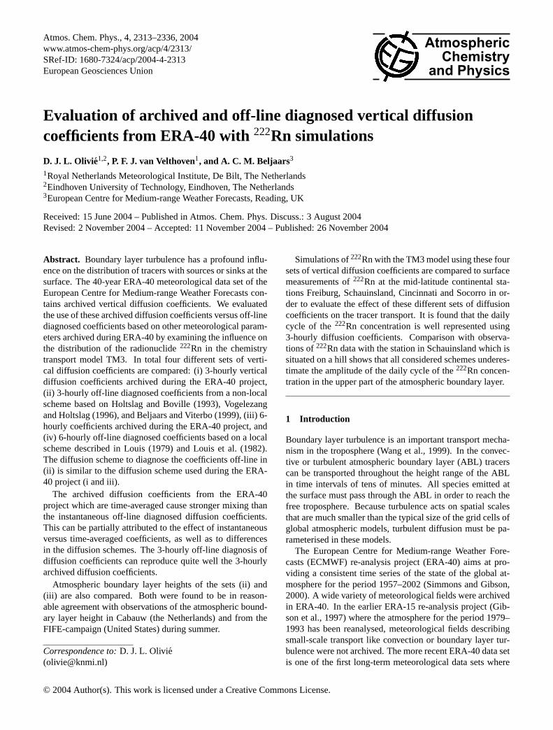
Zonally averagedKz profiles from the E3E6 scheme the H3scheme and the L6 scheme are shown in Fig2 for Januaryand July 1993 High values between the surface and 600 hPacorrespond to the presence of an ABL a local maximumaround 300 hPa corresponds to strong vertical wind gradi-ents in the upper troposphere Between 900 and 600 hPa overland the 90-percentileKz value is almost a factor 10 smallerin winter than during summer The largest differences be-tween the data sets can be found above the ABL In the freeatmosphere the L6 diffusion coefficients are 2 to 3 orders ofmagnitude larger than the H3 diffusion coefficients This ismainly due to the difference in the asymptotic mixing length450 m in the L6 case 30 m in the H3 case The E3E6 co-
efficients in the free atmosphere have values between the L6and H3 case
We studied time series ofKz at many different sites As anexample Figs3 4 and5 give time series of theKz profilein the lowest 3 km of the atmosphere at 3 different locationsat 80 E and 20 N (India) in January 1993 at 140 E and20 S (Australia) in January 1993 and at 150 W and 30 N(Pacific Ocean) in July 1993 In the ABL the profile ofKz
in the H3 case is very similar to the E3E6 case The ver-tical extent of the intenseKz values is a bit smaller than inthe E3E6 case In the H3 case the values are also slightlyless intense except in the winter over the continent at mid-latitudes Also in these time series one can observe the verylow values in the free troposphere in the H3 case There is aslightly higher variability in the E3 than in the H3 case (seeFig 5) which might be due to the archival ofKz (E3) versusoff-line diagnosis ofKz (H3) only every 6 h new profiles oftemperature humidity and wind are used in the H3 case
The Kz value in the L6 case differs often strongly fromthe other data sets At mid-latitudes E6 is much stronger inwinter Above sea the vertical extent of the ABL is muchsmaller (see Fig5) Also the profile ofKz is sometimes verydifferent because one finds locally sometimes very highKz
values in the L6 profile above sea (see Fig5) in the sub-tropics over land in the upper part of the ABL (see Fig4)
Atmos Chem Phys 4 2313ndash2336 2004 wwwatmos-chem-physorgacp42313
D J L Olivie et al Vertical diffusion coefficients from ERA-40 2321
Kz [m2s] E3-case
0 1 2 3 4 5 6 7 8 9 10 11 12 13 14 15time [day]
0
1
2
3
altit
ude
[km
]
Kz [m2s] H3-case
0 1 2 3 4 5 6 7 8 9 10 11 12 13 14 15time [day]
0
1
2
3
altit
ude
[km
]
Kz [m2s] E6-case
0 1 2 3 4 5 6 7 8 9 10 11 12 13 14 15time [day]
0
1
2
3
altit
ude
[km
]
Kz [m2s] L6-case
0 1 2 3 4 5 6 7 8 9 10 11 12 13 14 15time [day]
0
1
2
3
altit
ude
[km
]
001
003
010
030
100
300
1000
3000
10000
30000
100000
[m2s]300000
Fig 5 Time series of
-profile [m
s] in lowest 3 km of the atmosphere at 150W and 30
N (Pacific Ocean)
from 1 until 15 July 1993
32
Fig 5 Time series ofKz profile [m2s] in lowest 3 km of the atmosphere at 150 W and 30 N (Pacific Ocean) from 1 until 15 July 1993
or as disconnected spots in Fig3 Although the strong de-viation for the L6 case which is caused by the local natureof the scheme there is still a strong similarity with the otherKz profiles This is due to the fact that the L6Kz valuesare based on atmospheric profiles of temperature humidityand wind which carry the imprint of the ABL scheme usedduring ERA-40
32 Evaluation of the model simulated atmospheric bound-ary layer height
We compared the 6-hourly ABL height from the ERA-40data (E6) and the 3-hourly ABL height diagnosed in theH3-scheme with ABL heights observed in Cabauw and dur-ing the FIFE campaign The calculated and measured ABLheights during the FIFE campaign are shown in Fig6 (onlya subset of the data is shown) for Cabauw they are shown inFig 7 (all data is shown) The maximum value of the heightof the ABL is quite well represented both for the E6 and H3case Also the time of strongest growth and decrease is wellrepresented
Figure8 gives a scatter plots of the measured ABL heightduring the FIFE campaign versus the modelled ABL heightfor the cases E6 and H3 separately A distinction is madebetween measurements made during daytime and measure-ments made during nighttime At the end of the day (obser-
vations before 2100 LT) we see that the observations andmeasurements do not correspond very well (the model ABLheight is much larger) At this time of the day the ABL ishard to define anyway a stable inversion layer is building upbelow the residual layer Later during the night we see thatthe agreement between the observations and model is muchbetter It is clearly visible in Fig8 that the ABL height withlow as well as with high wind speeds corresponds well be-tween model and observations The H3 case gives a betteragreement than the L6 case
Also during daytime there is a good agreement For bothcases (E6 and H3) the modelled ABL height is larger thanobserved the H3 ABL height corresponds however slightlybetter with the observations The higher ABL height in theE6 case can be caused by the smaller coefficient for the ex-cess of the parcel temperature under unstable conditions Italso shows that a 6-hourly resolution is rather coarse for de-scribing the ABL height evolution
Due to the limited amount of data in Cabauw we only lookat the time evolution of the ABL height in Fig7 We seethat the quality of the ERA-40 ABL height and the H3 ABLheight are similar for both schemes the ABL height in theafternoon falls off in the model sometimes too fast and is atnight sometimes too high Comparison of the ABL height be-tween model and observations is hampered by representation
wwwatmos-chem-physorgacp42313 Atmos Chem Phys 4 2313ndash2336 2004
2322 D J L Olivie et al Vertical diffusion coefficients from ERA-40
28- 5-1987
0 6 12 18 24time [hour]
00
05
10
15
20
25
altit
ude
[km
]
29- 5-1987
0 6 12 18 24time [hour]
00
05
10
15
20
25
altit
ude
[km
]
30- 5-1987
0 6 12 18 24time [hour]
00
05
10
15
20
25
altit
ude
[km
]
31- 5-1987
0 6 12 18 24time [hour]
00
05
10
15
20
25
altit
ude
[km
]
1- 6-1987
0 6 12 18 24time [hour]
00
05
10
15
20
25
altit
ude
[km
]
2- 6-1987
0 6 12 18 24time [hour]
00
05
10
15
20
25
altit
ude
[km
]
3- 6-1987
0 6 12 18 24time [hour]
00
05
10
15
20
25
altit
ude
[km
]
4- 6-1987
0 6 12 18 24time [hour]
00
05
10
15
20
25al
titud
e [k
m]
5- 6-1987
0 6 12 18 24time [hour]
00
05
10
15
20
25
altit
ude
[km
]
6- 6-1987
0 6 12 18 24time [hour]
00
05
10
15
20
25
altit
ude
[km
]
25- 6-1987
0 6 12 18 24time [hour]
00
05
10
15
20
25
altit
ude
[km
]
26- 6-1987
0 6 12 18 24time [hour]
00
05
10
15
20
25
altit
ude
[km
] 27- 6-1987
0 6 12 18 24time [hour]
00
05
10
15
20
25
altit
ude
[km
]
28- 6-1987
0 6 12 18 24time [hour]
00
05
10
15
20
25
altit
ude
[km
]
29- 6-1987
0 6 12 18 24time [hour]
00
05
10
15
20
25
altit
ude
[km
]
30- 6-1987
0 6 12 18 24time [hour]
00
05
10
15
20
25
altit
ude
[km
]
1- 7-1987
0 6 12 18 24time [hour]
00
05
10
15
20
25
altit
ude
[km
]
2- 7-1987
0 6 12 18 24time [hour]
00
05
10
15
20
25
altit
ude
[km
]
3- 7-1987
0 6 12 18 24time [hour]
00
05
10
15
20
25
altit
ude
[km
]
4- 7-1987
0 6 12 18 24time [hour]
00
05
10
15
20
25
altit
ude
[km
]
5- 7-1987
0 6 12 18 24time [hour]
00
05
10
15
20
25
altit
ude
[km
]
6- 7-1987
0 6 12 18 24time [hour]
00
05
10
15
20
25
altit
ude
[km
]
7- 7-1987
0 6 12 18 24time [hour]
00
05
10
15
20
25
altit
ude
[km
]
8- 7-1987
0 6 12 18 24time [hour]
00
05
10
15
20
25
altit
ude
[km
]
Fig 6 Time evolution of the ABL height during the FIFE campaign in 1987 and 1989 in the US Pink stars de-
note the observed ABL height the dashed green line denotes the ABL height archived in the ERA-40 data (E6)
the dotted red line denotes the ABL height calculated in the H3-scheme The time is expressed in GMT+6h
33
Fig 6 Time evolution of the ABL height during the FIFE campaign in 1987 and 1989 in the US Pink stars denote the observed ABL heightthe dashed green line denotes the ABL height archived in the ERA-40 data (E6) the dotted red line denotes the ABL height calculated in theH3-scheme The time is expressed in GMT+6h
Atmos Chem Phys 4 2313ndash2336 2004 wwwatmos-chem-physorgacp42313
D J L Olivie et al Vertical diffusion coefficients from ERA-40 2323
5- 6-1996
0 6 12 18 24time [hour]
00
05
10
15
20
25al
titud
e [k
m]
11- 7-1996
0 6 12 18 24time [hour]
00
05
10
15
20
25
altit
ude
[km
]
15- 7-1996
0 6 12 18 24time [hour]
00
05
10
15
20
25
altit
ude
[km
]
16- 7-1996
0 6 12 18 24time [hour]
00
05
10
15
20
25
altit
ude
[km
]
17- 7-1996
0 6 12 18 24time [hour]
00
05
10
15
20
25
altit
ude
[km
]
19- 7-1996
0 6 12 18 24time [hour]
00
05
10
15
20
25
altit
ude
[km
]
2- 8-1996
0 6 12 18 24time [hour]
00
05
10
15
20
25
altit
ude
[km
]
4- 8-1996
0 6 12 18 24time [hour]
00
05
10
15
20
25
altit
ude
[km
] 5- 8-1996
0 6 12 18 24time [hour]
00
05
10
15
20
25
altit
ude
[km
]
15- 8-1996
0 6 12 18 24time [hour]
00
05
10
15
20
25
altit
ude
[km
]
19- 8-1996
0 6 12 18 24time [hour]
00
05
10
15
20
25
altit
ude
[km
]
22- 8-1996
0 6 12 18 24time [hour]
00
05
10
15
20
25
altit
ude
[km
]
Fig 7 Time evolution of the ABL height during some days in June July and August 1996 in Cabauw the
Netherlands Symbol and line code as in Figure 6 The time is expressed in GMT
34
Fig 7 Time evolution of the ABL height during some days in June July and August 1996 in Cabauw the Netherlands Symbol and linecode as in Fig6 The time is expressed in GMT
errors in modelled fluxes the presence of clouds during day-time and limited space and time resolution of the modelBosveld et al(1999) have compared observed heat fluxeswith modelled heat fluxes from ERA-15 at Cabauw Theyfound that the ECMWF model underestimates the amount ofclouds at Cabauw which leads to excessive surface heatingresulting in too large surface heat fluxes Similar deficienciesseem to be present in the ERA-40 data
Despite the rather limited comparison with measurementswe can conclude that the ABL heights as calculated duringthe ERA-40 project (E6) and with the H3 scheme agreereasonably with the measurements during summer in mid-latitudes
33 Comparison with222Rn measurements in Freiburg andSchauinsland
We compared the simulated222Rn concentrations from theTM3 model with surface observations from Freiburg andSchauinsland Time series of modelled and observed222Rnconcentrations are shown in Fig9 for the first 15 days ofJune and September 1993
Table 2 Mean value of the222Rn concentration [10minus21 molmol]in 1993 in Freiburg and Schauinsland
diffusion Freiburg Schauinsland
E3 102plusmn45 33plusmn15H3 110plusmn59 33plusmn16E6 98plusmn41 34plusmn15L6 125plusmn68 32plusmn16N 501plusmn113 26plusmn17
observed 113plusmn70 37plusmn19
331 Seasonal cycle of the modelled and measured222Rnconcentration
The monthly mean values of the222Rn concentration thecorrelation of the modelled with the observed daily mean val-ues and the correlation of the residues for the year 1993 inFreiburg and Schauinsland are shown in Fig10 (the residueis defined as the hourly concentration minus the daily meanconcentration) Table2 gives the 1993 yearly mean222Rn
wwwatmos-chem-physorgacp42313 Atmos Chem Phys 4 2313ndash2336 2004
2324 D J L Olivie et al Vertical diffusion coefficients from ERA-40
night time BLH case E6
00 05 10 15 20measurement [km]
00
05
10
15
20
mod
el [k
m]
y=026+065x
corr coeff=033
N=133
night time BLH case H3
00 05 10 15 20measurement [km]
00
05
10
15
20
mod
el [k
m]
y=006+125x
corr coeff=085
N=133
day time BLH case E6
00 05 10 15 20 25measurement [km]
00
05
10
15
20
25
mod
el [k
m]
y=061+081x
corr coeff=071
N=332
day time BLH case H3
00 05 10 15 20 25measurement [km]
00
05
10
15
20
25
mod
el [k
m]
y=027+093x
corr coeff=078
N=332
Fig 8 Scatter plot of the measured ABL height during the FIFE campaign versus the modelled ABL height
for E6 (left) and H3 (right) In the upper panel the nighttime observations are shown black signs refer to
measurements before 21h00 LT green signs (wind speed
3 ms) and red signs (wind speed 3 ms) refer
to measurements after 21h00 LT The regression line for the nighttime is only based on the observations after
21h00 LT In the lower panel the daytime observations are shown
35
Fig 8 Scatter plot of the measured ABL height during the FIFE campaign versus the modelled ABL height for E6 (left) and H3 (right)In the upper panel the nighttime observations are shown black signs refer to measurements before 2100 LT green signs (wind speedgt3ms) and red signs (wind speedlt3 ms) refer to measurements after 2100 LT The regression line for the nighttime is only based on theobservations after 2100 LT In the lower panel the daytime observations are shown
Table 3 Correlation of the modelled with the observed222Rn concentration in 1993 in Freiburg and Schauinsland In column (a) thecorrelation of the modelled with the observed daily mean is given in column (b) the correlation of the modelled with the observed hourlyvalue and in column (c) the correlation of the modelled with the observed residue (the residue is defined as the hourly concentration minusthe daily mean concentration)
diffusion Freiburg Schauinsland(a) (b) (c) (a) (b) (c)
(N=306) (N=7731) (N=7344) (N=243) (N=7250) (N=5832)
E3 0870 0773 0498 0589 0508 0282H3 0871 0790 0522 0528 0455 0242E6 0871 0759 0449 0596 0509 0262L6 0844 0735 0484 0538 0477 0286N 0704 0648 0364 0400 0347 0125
concentration All schemes reproduce the monthly meanvalues quite well both in Freiburg and in Schauinsland InFreiburg the spread in mean concentration between the dif-ferent diffusion schemes is about 20 The L6 scheme re-sults in the highest mean concentrations the E6 scheme inthe lowest mean concentrations The E3 case gives almostsimilar results as the E6 scheme In Schauinsland the spreadin the modelled result is much smaller (except in February)but the agreement with the measurements is smaller Forboth stations the correlation of the modelled with the ob-served mean daily value is higher than the correlation of themodelled with the observed hourly value (not shown) and
the correlation of the modelled with the observed residueis smallest It clearly shows that the variation of the222Rnconcentration by large scale synoptic variability is well mod-elled and that the variation of the222Rn concentration dueto local and short time scale phenomena (like diffusion) isharder to describe There is also a remarkable differencebetween the correlation of the modelled with the observedresidue between the E6 and the E3 case as well in Freiburgas Schauinsland Table3 gives the correlations between theobserved and modelled222Rn concentration during 1993
Atmos Chem Phys 4 2313ndash2336 2004 wwwatmos-chem-physorgacp42313
D J L Olivie et al Vertical diffusion coefficients from ERA-40 2325
JUN 1993
0 1 2 3 4 5 6 7 8 9 10 11 12 13 14 15time [day]
0
50
100
150
200
250
300
conc
entr
atio
n [1
0-21 m
olm
ol]
JUN 1993
0 1 2 3 4 5 6 7 8 9 10 11 12 13 14 15time [day]
0
20
40
60
80
100
120
conc
entr
atio
n [1
0-21 m
olm
ol]
SEP 1993
0 1 2 3 4 5 6 7 8 9 10 11 12 13 14 15time [day]
0
50
100
150
200
250
300
conc
entr
atio
n [1
0-21 m
olm
ol]
SEP 1993
0 1 2 3 4 5 6 7 8 9 10 11 12 13 14 15time [day]
0
20
40
60
80
100
120
conc
entr
atio
n [1
0-21 m
olm
ol]
Fig 9 Time series of
Rn concentration [10 molmol] in first 15 days of June and September 1993 for
Freiburg (1st and 3rd panel) and Schauinsland (2nd and 4th panel) The pink stars denote the observations the
lines denote the results from the model runs using E3 data (black line) using H3 data (red line) using E6 data
(green line) using L6 data (blue line) and using no diffusion (yellow line)36
Fig 9 Time series of222Rn concentration [10minus21 molmol] in first 15 days of June and September 1993 for Freiburg (1st and 3rd panel)and Schauinsland (2nd and 4th panel) The pink stars denote the observations the lines denote the results from the model runs using E3data (black line) using H3 data (red line) using E6 data (green line) using L6 data (blue line) and using no diffusion (yellow line)
332 Daily cycle
The mean daily cycle of the222Rn concentration in Freiburgand Schauinsland for December January and February (DJF)and for June July and August (JJA) are shown in Fig11 InFreiburg the daily cycle of the L6 case is largest The E3 andE6 cases are very similar except for the periods 600ndash900and 1500ndash2100 (only in DJF) where the E6 case results in
lower 222Rn values For all schemes the daytime concentra-tions are almost the same in JJA while differences persist inDJF
The daily cycle in the model simulations in Schauinslandis clearly not as strong as in the measurements The devi-ation is quite large in DJF In JJA the simulations repro-duce an increase in the concentration in the morning butnot large enough The schemes differ in the time positioning
wwwatmos-chem-physorgacp42313 Atmos Chem Phys 4 2313ndash2336 2004
2326 D J L Olivie et al Vertical diffusion coefficients from ERA-40
Mean 1993
J F M A M J J A S O N Dtime [month]
0
50
100
150
200
250
300
conc
entr
atio
n [1
0-21 m
olm
ol]
Mean 1993
J F M A M J J A S O N Dtime [month]
0
20
40
60
80
100
120
conc
entr
atio
n [1
0-21 m
olm
ol]
Mean correlation 1993
J F M A M J J A S O N Dtime (month)
00
02
04
06
08
10
corr
elat
ion
Mean correlation 1993
J F M A M J J A S O N Dtime (month)
00
02
04
06
08
10
corr
elat
ion
Residu correlation 1993
J F M A M J J A S O N Dtime (month)
00
02
04
06
08
10
corr
elat
ion
Residu correlation 1993
J F M A M J J A S O N Dtime (month)
00
02
04
06
08
10
corr
elat
ion
Fig 10 Monthly mean
Rn concentration (upper panels) correlation of the modelled with the observed
mean daily value (middle panels) and correlation of the observed with the modelled deviation (lower panels)
for Freiburg (left) and Schauinsland (right) in 1993 The pink stars denote the mean observations the lines
denote the results from the model runs using E3 data (solid black line) using H3 data (dotted red line) using
E6 data (dashed green line) and using L6 data (dot-dashed blue line) The error bars (upper panels) show the
standard deviation of the observations
37
Fig 10Monthly mean222Rn concentration (upper panels) correlation of the modelled with the observed mean daily value (middle panels)and correlation of the observed with the modelled deviation (lower panels) for Freiburg (left) and Schauinsland (right) in 1993 The pinkstars denote the mean observations the lines denote the results from the model runs using E3 data (solid black line) using H3 data (dottedred line) using E6 data (dashed green line) and using L6 data (dot-dashed blue line) The error bars (upper panels) show the 1σ standarddeviation of the observations
of this increase The second maximum in the measurementsin JJA in Schauinsland is clearly not present in the modelsimulations (except for the H3 case) In Fig11 one canclearly identify the times when the meteorological fields areupdated
The daily minimum daily maximum and daily amplitudeof the 222Rn concentration are closely related to the dailycycle of the ABL turbulence In Fig12 the monthly meanvalue of the daily minimum maximum and amplitude areshown It can be seen that in Freiburg these values corre-spond quite well with the measurements The amplitude isslightly overestimated by the L6 scheme while it is underes-timated by the E3 H3 and E6 scheme At the same time thecorrelation (not shown) of the modelled with the observeddaily amplitude is considerably smaller than the correlationof the modelled with the observed daily minimum or daily
maximum In Schauinsland we see that the minimum valuesin the model are in general higher than the observed mini-mum values that the maximum values are in general smallerthan the observed values and that the modelled amplitudeis therefore much smaller than the observed amplitude Theamplitude in the L6 case is largest In Schauinsland the vari-ation between the schemes is much smaller than in FreiburgAll this shows that the coarse time and spatial resolution ofthe model limit its ability to reproduce variations on shorttime scales
333 Ratio between222Rn concentration in Freiburg andSchauinsland
Because the stations at Freiburg and Schauinsland are closeto each other (12 km) and the station at Schauinsland lies
Atmos Chem Phys 4 2313ndash2336 2004 wwwatmos-chem-physorgacp42313
D J L Olivie et al Vertical diffusion coefficients from ERA-40 2327
DJF 1993
0 6 12 18 24time [hour]
0
50
100
150
200
250
300
conc
entr
atio
n [1
0-21 m
olm
ol]
JJA 1993
0 6 12 18 24time [hour]
0
50
100
150
200
250
300
conc
entr
atio
n [1
0-21 m
olm
ol]
DJF 1993
0 6 12 18 24time [hour]
0
20
40
60
80
100
120
conc
entr
atio
n [1
0-21 m
olm
ol]
JJA 1993
0 6 12 18 24time [hour]
0
20
40
60
80
100
120
conc
entr
atio
n [1
0-21 m
olm
ol]
Fig 11 Daily cycle of observed and modelled
Rn concentration in Freiburg in DJF (upper left) and JJA
(upper right) and in Schauinsland in DJF (lower left) and JJA (lower right) 1993 The stars denote the observed
value the lines denote the modelled values (line code is as in Figure 10) The error bars show the standard
deviation of the observations
38
Fig 11Daily cycle of observed and modelled222Rn concentration in Freiburg in DJF (upper left) and JJA (upper right) and in Schauinslandin DJF (lower left) and JJA (lower right) 1993 The stars denote the observed value the lines denote the modelled values (line code is as inFig 10) The error bars show the 1σ standard deviation of the observations
on a hill 900 m higher than Freiburg these stations are quitewell suited to study vertical concentration gradients in themodel Ideally we would prefer to use co-located observa-tions however tower measurements were not available to us
The ratio of the222 Rn concentration in Freiburg (300 mabove sea level) and Schauinsland(1200 m above sea level)is assumed to be less sensitive to errors in the222Rn emissionand to influences of large-scale transport (synoptic variabil-ity) In Fig 13 and Table4 the correlation between the ratioin the model and the ratio in the measurements is given Thisvalue of the correlation lies close to the correlation of thehourly value in Freiburg and is significantly higher than thecorrelation of the hourly concentration in Schauinsland (seeTable3)
Because we expect a strong dependence of the aforemen-tioned ratio on the ABL height we have grouped the mea-sured and modelled ratios as a function of the height of theABL For the height of the ABL we took the values of theABL height as they are calculated in the H3 scheme theyare calculated every 3 h and correspond well with observa-tions (see Sect32) Because the222Rn data are availablehourly we interpolated the ABL height to an hourly resolu-tion (We also tried this with the 6-hourly ABL heights fromthe ERA-40 data set We noticed however that this gave morenoisy relationships due to the coarser time resolution of theE6 ABL height)
In Fig 13 one can observe that the ratio becomes smalleras a function of the height of the ABL We would expect
Table 4 Correlation between the observed and modelled ratio ofthe222Rn concentration in Freiburg and in Schauinsland in 1993
diffusion FreiburgSchauinsland(N=6531)
E3 0758H3 0772E6 0741L6 0717N 0575
the ratio to go to one when the ABL height reaches higherthan the station in Schauinsland one expects hyperbolic be-haviour for ABL heights below 800ndash1000 m and a sharpdrop in the ratio around 800ndash1000 m We see however that aswell for the observed ratio as for the modelled ratio the tran-sition point is around 500 m and not around 800ndash1000 mThis can be related to the coarse vertical resolution between500 and 1000 m the large scatter of the data and the use ofa modelled ABL height to deduce these curves The E3E6scheme shows the strongest correspondence with the mea-surement the H3 and L6 scheme show the worst correspon-dence Also from this graph it is clear that the E3 and E6 casecause stronger mixing than the H3 and L6 case In generalthis Fig13shows that despite of the failure of the schemersquosto reproduce all the short time scale variations the mean vari-ations in the ratio are reasonably captured
wwwatmos-chem-physorgacp42313 Atmos Chem Phys 4 2313ndash2336 2004
2328 D J L Olivie et al Vertical diffusion coefficients from ERA-40
Minimum 1993
J F M A M J J A S O N Dtime [month]
0
50
100
150
200
250
300
conc
entr
atio
n [1
0-21 m
olm
ol]
Minimum 1993
J F M A M J J A S O N Dtime [month]
0
20
40
60
80
100
120
conc
entr
atio
n [1
0-21 m
olm
ol]
Maximum 1993
J F M A M J J A S O N Dtime [month]
0
50
100
150
200
250
300
conc
entr
atio
n [1
0-21 m
olm
ol]
Maximum 1993
J F M A M J J A S O N Dtime [month]
0
20
40
60
80
100
120
conc
entr
atio
n [1
0-21 m
olm
ol]
Amplitude 1993
J F M A M J J A S O N Dtime [month]
0
50
100
150
200
250
300
conc
entr
atio
n [1
0-21 m
olm
ol]
Amplitude 1993
J F M A M J J A S O N Dtime [month]
0
20
40
60
80
100
120
conc
entr
atio
n [1
0-21 m
olm
ol]
Fig 12 Monthly mean of the daily minimum (upper panels) daily maximum (middle panels) and daily am-
plitude (lower panels) in the
Rn concentration in Freiburg (left) and Schauinsland (right) in 1993 The stars
denote the measurements the lines denote the results from the model runs (line code as in Figure 10) The error
bars show the standard deviation of the observations
39
Fig 12 Monthly mean of the daily minimum (upper panels) daily maximum (middle panels) and daily amplitude (lower panels) in the222Rn concentration in Freiburg (left) and Schauinsland (right) in 1993 The stars denote the measurements the lines denote the results fromthe model runs (line code as in Fig10) The error bars show the 1σ standard deviation of the observations
Table 5 Correlation of the observed with the modelled222Rn con-centration in Cincinnati and Socorro
diffusion Cincinnati Socorromorning afternoon daily cycle(N=48) (N=48) (N=288)
H3 0523 0388 0823E6 0639 0399 0714L6 0711 0421 0759
334 Time shift
The diffusive and convective mass fluxes are updated in theTM3 model every 3 or 6 h The updates have a strong influ-ence on the modelled222Rn distribution (see Fig11) Thesimulations show that the more frequent the updates are the
better the correspondence with the measurements is E3 per-forms better than E6 H3 performs better than L6
Averaging of diffusion coefficients over a certain time in-terval leads to a strong influence of the large diffusion co-efficients during a part of this interval on the time-averageddiffusion coefficient and thus on the concentration and trans-port in the tracer transport model If one compares the E6 andE3 case it shows up as an earlier start and a sustained prolon-gation of the low daytime222Rn values in Freiburg (see againFig11) Using instantaneous diffusion coefficients can max-imally lead to a time shift of half the time step while usinga time-averaged value can lead in the extreme case to a timeshift of almost the whole time step This has a considerableinfluence in case of time steps of 6 h This might also play animportant role for other tracers than222Rn where chemistryand dry deposition come into play
Atmos Chem Phys 4 2313ndash2336 2004 wwwatmos-chem-physorgacp42313
D J L Olivie et al Vertical diffusion coefficients from ERA-40 2329
Ratio correlation 1993
J F M A M J J A S O N Dtime (month)
00
02
04
06
08
10
corr
elat
ion
1993
00 05 10 15 20 25boundary layer height [km]
0
2
4
6
8
10
conc
entr
atio
n ra
tio
Fig 13 Left panel correlation of the modelled with the observed ratio of the concentration in Freiburg and
the concentration in Schauinsland Right panel mean ratio between the
Rn concentration in Freiburg and
the concentration in Schauinsland as a function of the ABL height (calculated with the H3 scheme) for the year
1993 The thick pink line denotes the ratio derived from the observed concentrations the other lines denote
the ratiorsquos derived from the modelled concentrations using E3 data (solid black line) using H3 data (dotted red
line) using E6 data (dashed green line) and using L6 data (dot-dashed blue line) To calculate these curves
we binned all the hourly ABL height data in 15 bins with a width of 150 m ranging from 0 up to 2250 m The
ABL height is taken from the H3 scheme The error bars denote the standard deviation of the ratio derived
from the observed concentrations
MAM 1993
-12 -9 -6 -3 0 3 6 9 12timeshift [hour]
00
02
04
06
08
10
corr
elat
ion
JJA 1993
-12 -9 -6 -3 0 3 6 9 12timeshift [hour]
00
02
04
06
08
10
corr
elat
ion
Fig 14 The correlation of the hourly modelled with the hourly observed
Rn concentration in Freiburg in
MAM (left) and JJA (right) as a function of the time shift Only the modelled concentration between 0h00 and
12h00 GMT is used Values in the right hand part of the figure (positive time shifts) give the correlation of
model concentrations with a later observation values in the left part of the figure (negative time shifts) give the
correlation of model concentrations with an earlier observation Line code using E3 data (solid black line)
using H3 data (dotted red line) using E6 data (dashed green line) and using L6 data (dot-dashed blue line)
40
Fig 13Left panel correlation of the modelled with the observed ratio of the concentration in Freiburg and the concentration in SchauinslandRight panel mean ratio between the222Rn concentration in Freiburg and the concentration in Schauinsland as a function of the ABL height(calculated with the H3 scheme) for the year 1993 The thick pink line denotes the ratio derived from the observed concentrations the otherlines denote the ratiorsquos derived from the modelled concentrations using E3 data (solid black line) using H3 data (dotted red line) using E6data (dashed green line) and using L6 data (dot-dashed blue line) To calculate these curves we binned all the hourly ABL height data in15 bins with a width of 150 m ranging from 0 up to 2250 m The ABL height is taken from the H3 scheme The error bars denote the 1σ
standard deviation of the ratio derived from the observed concentrations
Ratio correlation 1993
J F M A M J J A S O N Dtime (month)
00
02
04
06
08
10
corr
elat
ion
1993
00 05 10 15 20 25boundary layer height [km]
0
2
4
6
8
10
conc
entr
atio
n ra
tio
Fig 13 Left panel correlation of the modelled with the observed ratio of the concentration in Freiburg and
the concentration in Schauinsland Right panel mean ratio between the
Rn concentration in Freiburg and
the concentration in Schauinsland as a function of the ABL height (calculated with the H3 scheme) for the year
1993 The thick pink line denotes the ratio derived from the observed concentrations the other lines denote
the ratiorsquos derived from the modelled concentrations using E3 data (solid black line) using H3 data (dotted red
line) using E6 data (dashed green line) and using L6 data (dot-dashed blue line) To calculate these curves
we binned all the hourly ABL height data in 15 bins with a width of 150 m ranging from 0 up to 2250 m The
ABL height is taken from the H3 scheme The error bars denote the standard deviation of the ratio derived
from the observed concentrations
MAM 1993
-12 -9 -6 -3 0 3 6 9 12timeshift [hour]
00
02
04
06
08
10
corr
elat
ion
JJA 1993
-12 -9 -6 -3 0 3 6 9 12timeshift [hour]
00
02
04
06
08
10co
rrel
atio
n
Fig 14 The correlation of the hourly modelled with the hourly observed
Rn concentration in Freiburg in
MAM (left) and JJA (right) as a function of the time shift Only the modelled concentration between 0h00 and
12h00 GMT is used Values in the right hand part of the figure (positive time shifts) give the correlation of
model concentrations with a later observation values in the left part of the figure (negative time shifts) give the
correlation of model concentrations with an earlier observation Line code using E3 data (solid black line)
using H3 data (dotted red line) using E6 data (dashed green line) and using L6 data (dot-dashed blue line)
40
Fig 14The correlation of the hourly modelled with the hourly observed222Rn concentration in Freiburg in MAM (left) and JJA (right) as afunction of the time shift Only the modelled concentration between 000 and 1200 GMT is used Values in the right hand part of the figure(positive time shifts) give the correlation of model concentrations with a later observation values in the left part of the figure (negative timeshifts) give the correlation of model concentrations with an earlier observation Line code using E3 data (solid black line) using H3 data(dotted red line) using E6 data (dashed green line) and using L6 data (dot-dashed blue line)
We have investigated this effect by correlating the mod-elled morning concentrations (from 000 until 1200 GMT)with time-shifted observed concentrations The correlationas a function of the applied time shift is shown in Fig14 forthe periods March-April-May (MAM) and JJA The strongesttime shift is found for the E6 and E3 case (E6 stronger thanE3) which both use time-averaged diffusion coefficientsThe time shift is smallest for the L6 and H3 case (instan-taneous values) With an applied time shift for the morningconcentrations of 3 h for the E3 case and up to 4 or 5 h inthe E6 case the E3 and E6 case perform equally good (JJA)or better (MAM) than the H3 scheme We have also cor-related the modelled afternoon concentrations (from 1200until 2400) with time-shifted observed concentrations Thisresulted in slightly smaller time shifts with the highest cor-relation for shifts back in time in the E6 and E3 case (cor-responding to persistent low222Rn concentrations at the end
of the day) Due to the opposite sign of the shifts betweenmorning and afternoon and due to a probable geographicaldependence of this shift it is not easy to implement a rem-edy It shows the necessity of high sampling frequency ofdata
34 Comparison with222Rn measurements in Cincinnatiand Socorro
Figure 15 gives the observed and modelled monthly meansurface concentration in Cincinnati for 800 and 1500 LTfrom January 1959 until February 1963 The seasonal vari-ation in the observations is much larger than in the modelGold et al(1964) attribute this to freezing minimizing theemission in winter and to an increasing emanation rate of222Rn due to the decrease of the moisture content of the soilwith increase of temperature in summer This dependence
wwwatmos-chem-physorgacp42313 Atmos Chem Phys 4 2313ndash2336 2004
2330 D J L Olivie et al Vertical diffusion coefficients from ERA-40
Morning
J F M A M J J A S O N D J F M A M J J A S O N D J F M A M J J A S O N D J F M A M J J A S O N D J Ftime [month]
0
100
200
300
400
500
conc
entr
atio
n [1
0-21 m
olm
ol]
Afternoon
J F M A M J J A S O N D J F M A M J J A S O N D J F M A M J J A S O N D J F M A M J J A S O N D J Ftime [month]
0
50
100
150
200
conc
entr
atio
n [1
0-21 m
olm
ol]
Morning
0 100 200 300 400 500measurement concentration [10-21 molmol]
0
100
200
300
400
500
mod
el c
once
ntra
tion
[10-2
1 mol
mol
] Afternoon
0 50 100 150 200 250measurement concentration [10-21 molmol]
0
50
100
150
200
250
mod
el c
once
ntra
tion
[10-2
1 mol
mol
]
Fig 15 Monthly mean morning (upper panel) and afternoon (middle panel)
Rn concentration from January
1959 until February 1963 at Cincinnati Observed concentrations (pink stars) and modelled concentrations
using H3 data (dotted red line) E6 data (dashed green line) and L6 (dot-dashed blue line) are shown Scatter
plots of the monthly mean morning (lower left) and afternoon (lower right)
Rn concentration are shown
using H3 data (red triangles) using E6 data (green squares) and using L6 data (blue diamonds)
41
Fig 15 Monthly mean morning (upper panel) and afternoon (middle panel)222Rn concentration from January 1959 until February 1963at Cincinnati Observed concentrations (pink stars) and modelled concentrations using H3 data (dotted red line) E6 data (dashed greenline) and L6 (dot-dashed blue line) are shown Scatter plots of the monthly mean morning (lower left) and afternoon (lower right)222Rnconcentration are shown using H3 data (red triangles) using E6 data (green squares) and using L6 data (blue diamonds)
of the emanation of222Rn on meteorological conditions isnot included in the TM3 model The poor correspondence ofthe morning data is probably also caused by a bad represen-tation of the night and morning222Rn profiles in the globalmodel due to the large thickness of the lowest model layer(about 60 m) resulting in lower modelled222Rn concentra-tions under very stable meteorological conditions Anothermain reason for discrepancy is that the morning measure-ments represent more local conditions which may not fulfilthe 1 atom cmminus2 sminus1 emission rate Although the observedmorning concentration is quite different from the modelledmorning concentration the afternoon concentrations agreequite well with the observations (see Fig15) As for the222Rn concentrations in Freiburg we see that the L6 schemeleads to the highest morning concentrations while the E6case gives the lowest values The H3 case gives intermediatevalues
Measurements of222Rn have been made at Socorro fromNovember 1951 until June 1957 These data were used togenerate monthly mean daily cycles of the222Rn concen-tration (Wilkening 1959) We have compared the monthlymean daily cycles from January 1959 until February 1963with these data The result can be seen in Fig16 The after-noon values for E6 L6 and H3 are very similar The meanvalues are given in Table6
35 Global222Rn distribution
In order to see the effect of diffusive transport on the freetroposphere concentrations of tracers we now consider thebudgets and transport of222Rn Diffusion leads in gen-eral to differences of up to 30 in the zonal mean222Rnconcentration compared to the case where no diffusion isapplied in the TM3 model Smaller diffusion coefficients
Atmos Chem Phys 4 2313ndash2336 2004 wwwatmos-chem-physorgacp42313
D J L Olivie et al Vertical diffusion coefficients from ERA-40 2331
JAN
0 6 12 18 24time [hour]
050
100150200250300
conc
entr
atio
n [1
0-21 m
olm
ol]
FEB
0 6 12 18 24time [hour]
050
100150200250300
conc
entr
atio
n [1
0-21 m
olm
ol]
MAR
0 6 12 18 24time [hour]
050
100150200250300
conc
entr
atio
n [1
0-21 m
olm
ol]
APR
0 6 12 18 24time [hour]
050
100150200250300
conc
entr
atio
n [1
0-21 m
olm
ol]
MAY
0 6 12 18 24time [hour]
050
100150200250300
conc
entr
atio
n [1
0-21 m
olm
ol]
JUN
0 6 12 18 24time [hour]
050
100150200250300
conc
entr
atio
n [1
0-21 m
olm
ol]
JUL
0 6 12 18 24time [hour]
050
100150200250300
conc
entr
atio
n [1
0-21 m
olm
ol]
AUG
0 6 12 18 24time [hour]
050
100150200250300
conc
entr
atio
n [1
0-21 m
olm
ol]
SEP
0 6 12 18 24time [hour]
050
100150200250300
conc
entr
atio
n [1
0-21 m
olm
ol]
OCT
0 6 12 18 24time [hour]
050
100150200250300
conc
entr
atio
n [1
0-21 m
olm
ol]
NOV
0 6 12 18 24time [hour]
050
100150200250300
conc
entr
atio
n [1
0-21 m
olm
ol]
DEC
0 6 12 18 24time [hour]
050
100150200250300
conc
entr
atio
n [1
0-21 m
olm
ol]
Fig 16 Monthly mean daily cycle of
Rn concentration from January 1959 until February 1963 in Socorro
measured (thick solid pink line) and modelled using H3 (dotted red line) using E6 (dashed green line) and using
L6 (dot-dashed blue line) The observed monthly mean daily cycles are based on measurements from November
1951 until June 1957 The error bars denote the standard deviation of the modelled concentration42
Fig 16 Monthly mean daily cycle of222Rn concentration from January 1959 until February 1963 in Socorro measured (thick solid pinkline) and modelled using H3 (dotted red line) using E6 (dashed green line) and using L6 (dot-dashed blue line) The observed monthlymean daily cycles are based on measurements from November 1951 until June 1957 The error bars denote the 1σ standard deviation of themodelled concentration
wwwatmos-chem-physorgacp42313 Atmos Chem Phys 4 2313ndash2336 2004
2332 D J L Olivie et al Vertical diffusion coefficients from ERA-40
Table 6 Mean observed and modelled222Rn concentration[10minus21 molmol] at Socorro The observations have been made be-tween November 1951 and June 1957 The modelled concentrationsare mean values for the period January 1959 until December 1962
diffusion Socorro
H3 113plusmn44E6 91plusmn44L6 121plusmn44
observed 158
lead to higher222Rn concentration in the lowest layers andhigher concentrations higher up in the atmosphere The in-fluence of diffusion is strongest in the parts of the atmospherewith strong downward large-scale motion like the subtropicsandor where there is no vertical mixing by convection InFig 17 the relative difference in the zonal mean222Rn con-centration between the E3 and H3 case and between the E3and L6 case is shown for DJF 1993
In Fig 18 the relative difference in222Rn concentrationsat 700 hPa between the E3 and H3 case and between the E3and L6 case is shown for JJA 1993
If we compare the E6 and E3 case the zonal mean differ-ences are everywhere smaller than 1 (not shown)
If we compare H3 and L6 with E3 we always see that the222Rn concentration in the lowest 500ndash1000 m is lower forE3 while above 1 km it is higher for E3 This higher concen-tration for H3 and L6 in the lowest layers of the atmosphereleads to higher222Rn concentrations in the upper troposphereby convection which transports the surface air to high alti-tudes in the tropics We see in JJA around the North Polehigher concentrations in the lowest kilometre in the E3 caseBecause there is almost no222Rn emission north of 60 Nthe concentration is higher in the free troposphere than at thesurface (via long range transport) The increased mixing inthe E3 case will then transport this222Rn downward
If we compare the H3 and E3 case we see much higherconcentrations in the E3 case in almost the whole tropo-sphere (except the lowest layers) The stronger diffusiongives more mixing Large differences can be found around700 hPa in the winter subtropics ie around 20 N in DJFand around 20 S in JJA
If we compare L6 and E3 we see the effect of strongerdiffusion in the free troposphere in the winter subtropics forL6 Through more intense and higher mixing the222Rn con-centrations are 5 to 10 higher around 500 hPa and 15lower around 800 hPa in DJF around 20 N and in JJA around20 S
Because222Rn has a short lifetime (about 55 days) wecan deduce the global mean net vertical222Rn transport andchanges therein due to differences in the diffusion schemesfrom its mean distribution The net flux profile of222Rn isan indication of how the vertical diffusion will affect other
tracers This flux strongly depends on the source character-istics of the tracer (which are uniform on the continent for222Rn) and it is also strongly dependent on the sinks and thelifetime In Fig 19 we show the net global vertical222Rnfluxes All fluxes are expressed relative to the E3 case Thedifferences in net global transport are maximally 4 Thedifference is largest around 900 hPa The difference betweenE3 and E6 are less than 1 The net transport for the H3 caseis stronger than the E3 case above 500 hPa and stronger forthe L6 case than the E3 case above 700 hPa The interactionbetween the convection and the ABL turbulence is clearlyvisible One can observe the following pattern weaker trans-port in the lower troposphere leads to stronger transport inand into the upper troposphere As mentioned before if theturbulent transport is weaker more222Rn remains in the low-est atmospheric levels which can then be transported to theupper troposphere via fast convective transport Higher con-centrations at the surface (due to less turbulent transport) thuslead to higher concentrations in the upper troposphere
In general one can see in Fig19 that the differences inconcentration and transport are quite small This can partlybe attributed to the fact that diffusion is not the only way ofvertical transport If the diffusive transport changes it willbe partly compensated by convective or large-scale verticaltransport
4 Conclusions
We have studied the application of archived and off-line diag-nosed vertical diffusion coefficient from the ERA-40 projectfor making simulations with chemistry transport models Wecompared 4 sets of vertical diffusion coefficients (E3) 3-hourly archived coefficients based on a non-local scheme(H3) 3-hourly off-line diagnosed coefficients based on a non-local scheme (E6) as E3 but 6-hourly values and (L6) 6-hourly off-line diagnosed coefficients based on a local diffu-sion scheme We also compared the ABL height of the setsE6 and H3
With the results of these comparisons in mind we wantto return to our research questions Comparison with ABLheight measurements shows that the ABL height (question1) archived in ERA-40 (E6) and the ABL height from the3-hourly off-line non-local scheme (H3) are in reasonableagreement with the ABL height observations performed inCabauw and during the FIFE campaign The time resolu-tion of 3 h makes the H3 ABL height more valuable than the6-hourly E6 ABL height
Vertical diffusion coefficients can be calculated accuratelyoff-line (question 2a) The off-line diagnosed set of non-local diffusion coefficients (H3) is based on a parameteri-sation that is very similar to the parameterisation used inthe ECMWF model to generate the archived diffusion co-efficients (E3E6) We find that the results are quite sim-ilar between the E3 and H3 case (both with 3-hourly time
Atmos Chem Phys 4 2313ndash2336 2004 wwwatmos-chem-physorgacp42313
D J L Olivie et al Vertical diffusion coefficients from ERA-40 2333
Fig 17 Zonal mean relative difference () in
Rn concentration between E3 and H3 (upper panel) and
between E3 and L6 (lower panel) for DJF 199343
Fig 17 Zonal mean relative difference () in222Rn concentrationbetween E3 and H3 (upper panel) and between E3 and L6 (lowerpanel) for DJF 1993
resolution) and that the apparent difference can be attributedto small differences in the implementation of the parame-terisation (different asymptotic mixing length different sta-bility functions present or absent detrainment formulation)Hence the off-line diagnosis of diffusion coefficients repro-duces quite well the archived diffusion coefficients
TheKz values from the local scheme in the L6 case (ques-tion 2b) were sometimes quite different from the non-localscheme E6 Although the mean values of the diffusion co-efficients in the lower troposphere were larger for the L6case than for the E6 case the instantaneous values led tosmaller ABL transport This could be attributed to the factthat the daytime222Rn concentrations are not very sensitiveto the much larger daytime L6 diffusion coefficients whilethe smaller night time diffusion coefficients have a strongimpact on the night concentration Sometimes theKz val-ues of L6 and E6 were still surprisingly similar This is due
Fig 18 The relative difference () in
Rn concentration at 700 hPa between E3 and H3 (upper panel) and
between E3 and L6 (lower panel) for DJF 1993
44
Fig 18 The relative difference () in222Rn concentration at700 hPa between E3 and H3 (upper panel) and between E3 andL6 (lower panel) for DJF 1993
to the fact that the underlying profiles of temperature humid-ity and wind to drive the off-line L6 scheme are taken fromthe ECMWF-model
Comparison of222Rn simulations from the TM3 modelwith surface222Rn observations in Freiburg SchauinslandCincinnati and Socorro shows that the 3-hourly E3 and H3(question 3a) schemes perform better than the 6-hourly E6and L6 schemes Using the 3-hourly coefficients results in abetter description of the daily cycle of the222Rn concentra-tion This might have an impact on tracers that undergo fastphotochemistry or are affected by dry deposition or vegeta-tion
It is also shown that using time-averaged diffusion coeffi-cients (question 3b) can lead to time shifts of the daily cycle
wwwatmos-chem-physorgacp42313 Atmos Chem Phys 4 2313ndash2336 2004
2334 D J L Olivie et al Vertical diffusion coefficients from ERA-40
DJF
08 09 10 11 12relative concentration
1000
800
600
400
200
0
pres
sure
(hP
a)
JJA
08 09 10 11 12relative concentration
1000
800
600
400
200
0
pres
sure
(hP
a)
DJF
0950 0975 1000 1025 1050relative tracer flux
1000
800
600
400
200
0
pres
sure
(hP
a)
JJA
0950 0975 1000 1025 1050relative tracer flux
1000
800
600
400
200
0
pres
sure
(hP
a)
Fig 19 Profiles of the global mean
Rn concentration (upper panels) and profiles of the global mean net
upward
Rn flux (lower panels) are shown for DJF and JJA 1993 The concentration and flux of E3 (solid
black) H3 (dotted red) E6 (dashed green) L6 (dot-dashed blue) are expressed with respect to the flux of E3
45
Fig 19Profiles of the global mean222Rn concentration (upper panels) and profiles of the global mean net upward222Rn flux (lower panels)are shown for DJF and JJA 1993 The concentration and flux of E3 (solid black) H3 (dotted red) E6 (dashed green) L6 (dot-dashed blue)are expressed with respect to the flux of E3
of tracer concentrations and stronger vertical transport thaninstantaneous diffusion coefficients
Finally some recommendations can be formulated Firstusing the E3 scheme resulted in higher222Rn concentrationsin the free troposphere than using the H3 scheme The sea-sonal zonal and monthly mean222Rn concentration can dif-fer up to 10 Earlier studies with the TM3 model suggestedthat vertical mixing was underestimated As mentioned be-fore this difference can be partially attributed to the use ofthe detrainment formulation at the top of the ABL for theE3 case a larger asymptotic mixing length and differencesin the stability functions It would be therefore worthwhilemaking these changes in the off-line H3-scheme
Secondly the non-local schemes that are used here do notcontain a counter gradient term Also here it could be in-teresting to investigate whether including the counter gradi-ent term could further improve the agreement with measure-ments
Finally the large discrepancy in222Rn concentration be-tween model and observations at some sites suggests that amore physical based emanation rate of222Rn and perhaps ahigher spatial resolution should be used
AcknowledgementsThis evaluation of diffusion coefficients wouldnot have been possible without the atmospheric monitoring workof Mr Sartorius from the Federal Office for Radiation Protection inFreiburg Germany who provided222Rn data from the locations
Freiburg and Schauinsland We thank H Klein Baltink for theABL height measurement data from Cabauw ECMWF ERA-40data used in this study have been provided by ECMWF Thiswork was supported by the Netherlands Organization for ScientificResearch (NWO) and by the European Union under contractnumber EVK2-CT-2002-00170 (RETRO)
Edited by F J Dentener
References
Allen D J Rood R B Thompson A M and Hudson R DThree-dimensional radon 222 calculations using assimilated me-teorological data and a convective mixing algorithm J GeophysRes D3 101 6871ndash6881 1996
Balkanski Y J and Jacob D J Transport of continental air to thesubantarctic Indian Ocean Tellus B 42 62ndash75 1990
Beljaars A C M and Viterbo P Role of the boundary layerin a numerical weather prediction model in Clear and cloudyboundary layers edited by Holtslag A A M and DuynkerkeP G pp 287ndash304 NH-publishers 1999
Bosveld F van Ulden A and Beljaars A C M A compari-son of ECMWF Re-Analysis data with fluxes and profiles ob-served in Cabauw ECMWF Re-Analysis Project Report Series 8ECMWF Reading RG2 9AX UK 1999
Bregman B Segers A Krol M Meijer E and van VelthovenP On the use of mass-conserving wind fields in chemistry trans-
Atmos Chem Phys 4 2313ndash2336 2004 wwwatmos-chem-physorgacp42313
D J L Olivie et al Vertical diffusion coefficients from ERA-40 2335
port models Atmos Chem Phys 3 447ndash457 2003SRef-ID 1680-7324acp2003-3-447
Broecker W S Li Y H and Cromwell J Radium-226 andradon-222 concentration in Atlantic and Pacific Oceans Science158 1307ndash1310 1967
Brost R A and Chatfield R B Transport of radon in a three-dimensional subhemispheric model J Geophys Res 94 5095ndash5119 1989
Dentener F Feichter J and Jeuken A Simulation of the trans-port of 222Rn using on-line and off-line global models at differ-ent horizontal resolutions a detailed comparison with measure-ments Tellus B 51 573ndash602 1999
Dentener F Peters W Krol M van Weele M Bergamaschi Pand Lelieveld J Interannual variability and trend of CH4 life-time as measure for OH changes in the 1979ndash1993 time periodJ Geophys Res 108 4442 doi1010292002JD002916 2003
Eloranta E W Boundary Layer Heights LIDAR (FIFE)Data set Available online [httpwwwdaacornlgov] from OakRidge National Laboratory Distributed Active Archive CenterOak Ridge Tennessee USA also published in Collected Dataof the First ISLSCP Field Experiment Vol 1 Surface Observa-tions and Non-Image Data Sets edited by Strebel D E Lan-dis D R Huemmrich K F and Meeson B W CD-ROMNational Aeronautics and Space Administration Goddard SpaceFlight Center Greenbelt Maryland USA 1994
Feichter J and Crutzen P J Parameterization of vertical transportdue to deep cumulus convection in a global transport model andits evaluation with222Radon measurements Tellus B 42 100ndash117 1990
Gibson J K Kallberg P Uppala S Hernandez A NomuraA and Serrano E ERA-15 description ECMWF Re-AnalysisProject Report Series 1 ECMWF Reading RG2 9AX UK1997
Gold S Barkhau H W Shleien B and Kahn B Measurementsof naturally occuring radionucleides in air in The Natural Ra-diation Environment edited by Adams J A S and LowderW M pp 369ndash382 University of Chicago Press Chicago Ill1964
Gregory D Morcrette J-J Jakob C Beljaars A C M andStockdale T Revision of convection radiation and cloudschemes in the ECMWF Integrated Forecasting System Q J RMeteor Soc 126 1685ndash1710 2000
Heimann M The global atmospheric tracer model TM2 TechRep 10 Deutsches Klimarechenzentrum Hamburg Germany1995
Holtslag A A M and Boville B A Local versus nonlocalboundary-layer diffusion in a global climate model J Climate6 1825ndash1842 1993
Holtslag A A M van Meijgaard E and de Rooy W C A com-parison of boundary layer diffusion schemes in unstable condi-tions over land Boundary-Layer Meteor 76 69ndash95 1995
Houweling A Dentener F and Lelieveld J The impact of non-methane hydrocarbon compounds on tropospheric photochem-istry J Geophys Res D9 103 10 673ndash10 696 1998
Jacob D J and Prather M J Radon-222 as a test of boundarylayer convection in a general circulation model Tellus B 42117ndash134 1990
Jacob D J Prather M J Rasch P J Shia R-L BalkanskiY L Beagley S R Bergmann D J Blackshear W T Brown
M Chiba M Chipperfield M P de Grandpre J DignonJ E Feichter J Genthon C Grose W L Kasibhatla P SKohler I Kritz M A Law K Penner J E Reeves M RC E Rotman D A Stockwell D Z van Velthoven P F JVerver G Wild O Yang H and Zimmerman P Evaluationand intercomparison of global transport models using222Rn andother short-lived tracers J Geophys Res D5 102 5953ndash59701997
Jeuken A Evaluation of chemistry and climate models usingmeasurements and data assimilation PhD thesis University ofTechnology Eindhoven Eindhoven The Netherlands availableathttpalexandriatuenlextra2200001283pdf 2000
Jeuken A Veefkind J P Dentener F Metzger S and GonzalesC R Simulation of the aerosol optical depth over Europe forAugust 1997 and a comparison with observations J GeophysRes D22 106 28 295ndash28 311 2001
Kritz M A Roulley J-C L and Danielsen E F The ChinaClipperndashfast advective transport of radon-rich air from the Asianboundary layer to the upper troposphere near California TellusB 42 46ndash61 1990
Lambert G Polian G Sanak J Ardouin B Buisson AJegou A and Roulley J C L Cycle du radon et de sesdescendants applicationa lrsquoetude desechanges troposphere-stratosphere Ann Geophys 4 38 497ndash531 1982
Lee H N and Larsen R J Vertical diffusion in the lower atmo-sphere using aircraft measurements of222Rn J Appl Meteorol36 1262ndash1270 1997
Lelieveld J and Dentener F What controls tropospheric ozoneJ Geophys Res D3 105 3531ndash3551 2000
Liu S C McAfee J R and Cicerone R J Radon 222 and tro-pospheric vertical transport J Geophys Res D5 7291ndash72971984
Louis J-F A parametric model of vertical eddy fluxes in the at-mosphere Bound-Layer Meteor 17 187ndash202 1979
Louis J F Tiedtke M and Geleyn J F A short history of the op-erational PBL-parameterization at ECMWF in Proceedings ofECMWF workshop on boundary layer parameterization Novem-ber 1981 59ndash79 ECMWF Reading England 1982
Mahowald N M Rasch P J Eaton B E Whittlestone S andPrinn R Transport of222radon to the remote troposphere usingthe Model of Atmospheric Transport and Chemistry and assimi-lated winds from ECMWF and the National Center for Environ-mental PredictionNCAR J Geophys Res D23 102 28 139ndash28 151 1997
Nordeng T E Extended versions of the convective parametriza-tion scheme at ECMWF and their impact on the mean and tran-sient activity of the model in the tropics Research DepartmentTechnical Memorandum 206 ECMWF Reading RG2 9AXUK 1994
Olivi e D J L van Velthoven P F J Beljaars A and KelderH M Comparison between archived and off-line diagnosedconvective mass fluxes in the chemistry transport model TM3 JGeophys Res D11 109 D11 303 doi1010292003JD0040362004
Polian G Lambert G Ardouin B and Jegou A Long-rangetransport of radon in subantarctic and antarctic areas Tellus B38 178ndash189 1986
Russell G L and Lerner J A A new finite-differencing schemefor the tracer transport equation J Appl Meteorol 20 1483ndash
wwwatmos-chem-physorgacp42313 Atmos Chem Phys 4 2313ndash2336 2004
2336 D J L Olivie et al Vertical diffusion coefficients from ERA-40
1498 1981Sellers P J Hall F G Asrar G Strebel D E and Murphy
R E The First ISLSCP Field Experiment (FIFE) Bull AmMeteor Soc 69 22ndash27 1988
Simmons A J and Burridge D M An energy and angular-momentum conserving vertical finite-difference scheme and hy-brid vertical coordinates Mon Weather Rev 109 758ndash7661981
Simmons A J and Gibson J K The ERA-40 project plan ERA-40 Project Report Series 1 ECMWF Reading RG2 9AX UK2000
Stockwell D Z and Chipperfield M P A tropospheric chemical-transport model development and validation of the model trans-port schemes Q J R Meteorol Soc 125 1747ndash1783 1999
Stockwell D Z Kritz M Chipperfield M P and Pyle J A Val-idation of an off-line three-dimensional chemical transport modelusing observed radon profiles 2 Model results J Geophys ResD7 103 8433ndash8445 1998
Tiedtke M A comprehensive mass flux scheme for cumulus pa-rameterization in large-scale models Mon Weather Rev 1171779ndash1800 1989
Troen I and Mahrt L A simple model of the atmospheric bound-ary layer sensitivity to surface evaporation Bound-Layer Me-teor 37 129ndash148 1986
Turekian K K Nozaki Y and Benninger L K Geochemistry ofatmospheric radon and radon products Ann Rev Earth PlanetSci 5 227ndash255 1977
Viterbo P Beljaars A Mahfouf J-F and Teixeira J The rep-resentation of soil moisture freezing and its impact on the stableboundary layer Q J R Meteor Soc 125 2401ndash2426 1999
Vogelezang D H P and Holtslag A A M Evaluation andmodel impacts of alternative boundary-layer height formulationsBound-Layer Meteor 81 245ndash269 1996
Wang K-Y Pyle J A Sanderson M G and Bridgeman C Im-plementation of a convective atmospheric boundary layer schemein a tropospheric chemistry transport model J Geophys ResD19 104 23 729ndash23 745 1999
Wesely M L Boundary Layer Heights SODAR (FIFE) Data setAvailable online [httpwwwdaacornlgov] from Oak RidgeNational Laboratory Distributed Active Archive Center OakRidge Tennessee USA also published in Collected Data ofthe First ISLSCP Field Experiment Vol 1 Surface Observa-tions and Non-Image Data Sets edited by Strebel D E Lan-dis D R Huemmrich K F and Meeson B W CD-ROMNational Aeronautics and Space Administration Goddard SpaceFlight Center Greenbelt Maryland USA 1994
Wilkening M H Daily and annual courses of natural atmosphericradioactivity J Geophys Res 64 521ndash526 1959
Wilkening M H and Clements W E Radon 222 from the oceansurface J Geophys Res 80 3828ndash3830 1975
Williamson D L Kiehl J T Ramanathan V Dickinson R Eand Hack J J Description of NCAR Community ClimateModel (CCM1) NCAR Technical Note 285 NCAR 1987
Atmos Chem Phys 4 2313ndash2336 2004 wwwatmos-chem-physorgacp42313

2314 D J L Olivie et al Vertical diffusion coefficients from ERA-40
vertical diffusion coefficients for heat are archived (availableas 3- or 6-hourly averaged values)
Meteorological data sets such as ERA-40 and ERA-15 arecommonly used to study the transport and chemical evolu-tion of atmospheric gases and aerosols in chemical transportmodels (CTMs) The chemical transport model TM3 (TracerModel Version 3) is a global atmospheric model which is ap-plied to evaluate the atmospheric composition and changesherein caused by natural and anthropogenic changes For de-scribing the turbulent transport it can use different turbu-lent diffusion data Until now two off-line vertical diffu-sion schemes have been used in the TM3 model where thediffusion coefficients are diagnosed off-line based on otherregularly (eg 6-hourly) archived meteorological fields Thefirst scheme based onLouis (1979) andLouis et al(1982)is a local diffusion scheme that describes the vertical diffu-sion coefficient as a function of a mixing length scale thelocal gradient of the wind and the virtual temperature How-ever under convective conditions when the largest trans-porting eddies may have sizes similar to the depth of theABL local schemes do not perform well (Troen and Mahrt1986) the characteristics of the large eddies are not properlytaken into account The second scheme based on a combi-nation ofHoltslag and Boville(1993) Vogelezang and Holt-slag(1996) andBeljaars and Viterbo(1999) is a non-localdiffusion scheme Non-local ABL schemes often contain aterm that describes counter gradient transport by the largeeddies (Troen and Mahrt 1986) and prescribe the shape ofthe vertical profile of the diffusion coefficient Apart fromthe meteorological fields needed for a local scheme a non-local scheme also uses the surface sensible and latent heatfluxes The vertical exchange has been shown to be morepronounced with non-local schemes than with local schemes(Holtslag and Boville 1993 Holtslag et al 1995) The3-hourly off-line scheme (Holtslag and Boville 1993 Vo-gelezang and Holtslag 1996 Beljaars and Viterbo 1999) iscurrently most used in the TM3 model The 6-hourly off-linescheme (Louis 1979 Louis et al 1982) was until recentlyused in the TM3 model for various studiesDentener et al(2003) used meteorological data from the ERA-15 project(which does not provide 3-hourly surface latent heat fluxes)and the 6-hourly off-line scheme (Louis 1979 Louis et al1982) From now on however the ERA-40 data set allowsthe use of archived vertical diffusion data (3-hourly or 6-hourly) in the TM3 model One of the first to use archivedsub-grid meteorological parameters wasAllen et al (1996)They used archived convective mass fluxes and detrainmentsas well as the ABL heights An advantage of the use ofarchived meteorological fields to describe small-scale trans-port in CTMs is the consistency of these fields with thearchived fields of cloud cover temperature humidity or pre-cipitation
The effect on the transport of tracers by the diffusion datacan be studied by making222Rn simulations with CTMs222Rn is an excellent tracer to study the transport character-
istics on short time scales (hours to weeks) because it hasan almost uniform emission rate over land and is only lostthrough radioactive decay with an e-folding lifetime of about55 days (Dentener et al 1999 Balkanski and Jacob 1990Kritz et al 1990 Brost and Chatfield 1989 Polian et al1986) Therefore222Rn has been used extensively to evaluateparameterisations of convective transport (Mahowald et al1997 Allen et al 1996 Feichter and Crutzen 1990 Jacoband Prather 1990) and ABL diffusion (Stockwell and Chip-perfield 1999 Stockwell et al 1998 Jacob et al 1997 Leeand Larsen 1997 Mahowald et al 1997) in atmosphericmodels
In this work we try to answer the following questions(1) How well is the mid-latitude summer time ABL height re-produced in the ERA-40 data and in an off-line model drivenby ERA-40 data (2a) Can diffusion coefficients be repro-duced accurately off-line for use in CTMs (2b) How dolocal ABL schemes perform versus non-local ABL schemeswhen applied off-line (3a) How crucial is a 3-hourly timeresolution for diffusion data for CTM-modelling (3b) Whatis the influence of using time-averaged diffusion coefficientson the tracer transport in CTMs
To answer these questions we will start with a descriptionof the TM3 model and the diffusion schemes that generatethe different sets of vertical diffusion coefficients (Sect 2)In that section we will also describe the222Rn emission sce-nario in the TM3 model the222Rn observations and theABL height observations In Sect 3 we will first comparethe vertical diffusion coefficients from the different schemesThen we will compare the modelled ABL height at two mid-latitude stations with observations Next we will compare the222Rn concentration which is modelled in the TM3 modelusing the different sets of diffusion data with surface mea-surements of the222Rn concentration at four selected surfacestations In Sect 4 we will formulate the conclusions andformulate some recommendations
2 Methods
21 The TM3 chemistry transport model
The chemical transport model TM3 (Tracer Model Version3) is a global atmospheric CTM with a regular longitude-latitude grid and hybridσ -pressure levels (Lelieveld andDentener 2000 Houweling et al 1998 Heimann 1995)The meteorological input data for TM3 from ERA-40 isavailable for 1957 to 2002 For dynamics calculationsERA-40 used a spectral truncation of T159 The physi-cal calculations were done on a reduced Gaussian grid of160 nodes (N80) In the vertical 60 hybridσ -pressure lev-els (Simmons and Burridge 1981) were used reaching upto 01 hPa To be used in the TM3 model the meteorologi-cal data is interpolated or averaged to the desired TM3 gridcells (Bregman et al 2003) For advection of the tracers
Atmos Chem Phys 4 2313ndash2336 2004 wwwatmos-chem-physorgacp42313
D J L Olivie et al Vertical diffusion coefficients from ERA-40 2315
the model uses the slopes scheme developed by Russel andLerner (Russell and Lerner 1981) To describe the effect ofconvective transport on the tracer concentration we used thearchived convective mass fluxes from the ERA-40 data set(Olivi e et al 2004) The convection scheme in the ECMWF-model used during the ERA-40 project is based onTiedtke(1989) Gregory et al(2000) andNordeng(1994)
The vertical diffusion of tracers in the TM3 model is de-scribed with a first order closure scheme The net turbulenttracer fluxwprimeχ prime is expressed as
minus wprimeχ prime = Kz
partχ
partz (1)
whereKz is the vertical diffusion coefficient for heatw thevertical velocityχ the tracer concentration andz the heightabove the surface It is assumed that the vertical diffusioncoefficient for tracers is equal to the vertical diffusion coeffi-cient for heat In contrast toHoltslag and Boville(1993) andWang et al(1999) there is no counter gradient term in theTM3 implementation
The vertical diffusion coefficients are applied in the TM3model by converting the vertical diffusion coefficients intoupward and downward vertical air mass fluxes of equal mag-nitude which model the exchange between two model layersThese air mass fluxes are combined with the vertical con-vective mass fluxes from the convection parameterisation tocalculate the sub-grid scale vertical tracer transport with animplicit numerical scheme This allows the time steps in theTM3 model to be rather large without introducing stabilityproblems In the case of very large time steps the effect ofthe scheme is that it pushes the tracer concentration at onceto its equilibrium distribution In this study we used a timestep of 1 h for the small-scale vertical transport
From Eq (1) one derives that the dimensions ofKz areL2Tminus1 Taking the ABL height as a representative lengthscale for the effect of diffusion gives a relationship betweenKz and the time scale of turbulent diffusion If for examplethe ABL height is 1000 m andKz is 300 m2s one finds atime scale of around 1 h This means that a tracer initiallyonly present at the surface will be well mixed throughoutthe complete ABL on a time scale of 1 h
22 Vertical diffusion data
Different sets of vertical diffusion coefficients are used in theTM3 model We will briefly describe the schemes that areused to calculate these data sets
221 The ERA-40 3-hourly and 6-hourly diffusion coeffi-cients
The scheme as it is used in the ERA-40 project is describedin the documentation of the cycle CY23r4 of the ECMWFmodel see httpwwwecmwfintresearchifsdocsCY23r4It is a non-local scheme The coefficients for vertical dif-
fusion of heat were stored during the ERA-40 project as 3-hourly averaged values They can also be combined to 6-hourly averaged values
Different formulations are used based on the stabilityregime that is determined by the virtual potential temperatureflux (wprimeθ prime
v)0 If the surface layer is unstable ((wprimeθ primev)0gt0)
then a method according toTroen and Mahrt(1986) is ap-plied This method determines the ABL heighth using aparcel method where the parcel is lifted from the minimumvirtual temperature rather than from the surface The dimen-sionless coefficient for the excess of the parcel temperatureis reduced from 65 (Troen and Mahrt 1986) or 85 (Holt-slag and Boville 1993) to 2 (to get a well controlled entrain-ment rate and a less aggressive erosion of inversions) In theABL the vertical profile of diffusion coefficients is prede-fined (Troen and Mahrt 1986)
Kz = κ wh z(1 minus
z
h
)2 (2)
where wh is a turbulent velocity scale andκ=04 theVon Karman constant At the top of the ABL there is an ex-plicit entrainment formulation in the capping inversion Thevirtual heat flux at the top of the ABL is taken proportionalto the surface virtual heat flux
(wprimeθ primev)h = minusC (wprimeθ prime
v)0 (3)
with C=02 andθv the virtual potential temperature Know-ing the flux the diffusion coefficient at the top of the ABLcan be expressed as
Kz = C(wprimeθ prime
v)0partθv
partz
(4)
wherepartθv
partzis the virtual potential temperature gradient in the
inversion layerIf the surface layer is stable ((wprimeθ prime
v)0lt0) the diffusion co-efficients are determined by the gradient Richardson numberRi which is defined as
Ri =g
θ
partθpartz∣∣∣ partvpartz
∣∣∣2 (5)
wherev is the horizontal wind velocity When the atmo-sphere is locally unstable (Rilt0) then
Kz =l2h
8m 8h
∣∣∣∣partv
partz
∣∣∣∣ (6)
where
8m(ζ ) = (1 minus 16ζ )minus14 (7)
and where
8h(ζ ) = (1 minus 16ζ )minus12 (8)
wwwatmos-chem-physorgacp42313 Atmos Chem Phys 4 2313ndash2336 2004
2316 D J L Olivie et al Vertical diffusion coefficients from ERA-40
whereζ is taken equal toRi The mixing lengthlh is calcu-lated according to
1
lh=
1
κ z+
1
λh
(9)
The asymptotic mixing lengthλh [m] is defined as
λh = 30+120
1 +(
z4000
)2 (10)
wherez [m] is the height above the surface The asymptoticmixing lengthλh is a typical length scale in a neutral atmo-sphere for the vertical exchange of some quantity (momen-tum heat or tracer) due to turbulent eddies In the lowestlayers of the atmosphere the size of the turbulent eddies islimited by the presence of the earthrsquos surface which is takeninto account in the mixing lengthlh in Eq (9)
When the atmosphere is locally stable (Rigt0) ζ is readfrom a table (ζ=ζ(Ri)) The diffusion coefficients are cal-culated with
Kz = l2h
∣∣∣∣partv
partz
∣∣∣∣ Fh(Ri) (11)
where the stability functionFh(Ri) is a revised function oftheLouis et al(1982) function (Beljaars and Viterbo 1999)
Fh(Ri) =1
1 + 2b Riradic
1 + d Ri (12)
whereb=5 andd=1 This formulation has less discrepancybetween momentum and heat diffusion the ratio of momen-tum and heat diffusion is reduced (Viterbo et al 1999) Theformulation ofKz in case of a stable surface layer also ap-plies to the formulation ofKz above the ABL in case of anunstable surface layer
The calculation of the atmospheric boundary layer heightstored during the ERA-40 project is also described in the in-formation about the cycle CY23r4 As well in the stablein the neutral as in the unstable case a parcel lifting methodproposed byTroen and Mahrt(1986) is used They use a crit-ical bulk Richardson numberRib=025 The bulk Richard-son number is based on the difference between quantities atthe level of interest and the lowest model level This ABLheight is available every 3 h and represents an instantaneousvalue We only studied the 6-hourly values We will referto these 3-hourly diffusion coefficients as E3 and to these6-hourly diffusion coefficients and 6-hourly ABL heights asE6
222 The TM3 off-line 3-hourly and 6-hourly diffusion co-efficients
The first set of off-line diagnosed diffusion coefficients inTM3 is calculated with a scheme that is rather similar tothe above-described scheme It is a non-local scheme basedon Holtslag and Boville(1993) Vogelezang and Holtslag
(1996) andBeljaars and Viterbo(1999) The diffusion co-efficients are calculated every 3 h based on 3-hourly latentand sensible heat fluxes and 6-hourly fields of wind tem-perature and humidity It has been implemented and testedin the TM3 model (Jeuken 2000 Jeuken et al 2001) ThecalculatedKz values are instantaneous values
Although the scheme is rather similar to the aforemen-tioned E3E6 scheme there are some differences (i) a bulkRichardson criterion instead of a parcel ascent method isused to determine the height of the ABL (ii) there is no en-trainment formulation at the top of the ABL (iii) the temper-ature excess of the large eddies under convective conditionsis larger (iv) the prescribed profile of the asymptotic mixinglength is different and (v) the stability functions are differ-ent
If the surface layer is unstable ((wprimeθ primev)0gt0) a prescribed
profile of the vertical diffusion coefficients as in Eq (2) isused According toVogelezang and Holtslag(1996) the ABLheighth is the layer where the bulk Richardson number
Rib =
gθvs
(θvh minus θvs)(h minus zs)
|vh minus vs |2 + b u2
lowast
(13)
reaches a critical valueRib=03 (in Vogelezang and Holtslag(1996) the critical value isRib=025) The indexs refers tovalues in the lowest model layer the indexh refers to valuesat the top of the ABLulowast is the friction velocity The valuefor b=100 The exact ABL height is calculated by linearinterpolation The temperature excess under convective con-ditions is calculated using a coefficient with value 85 (versus2 in the E3E6 case)
If the surface layer is stable ((wprimeθ primev)0lt0) the diffusion co-
efficients are calculated with Eq (11) When the atmosphereis locally stable (Rigt0) we take
Fh(Ri) =1
1 + 10Riradic
1 + Ri (14)
while when the atmosphere is locally unstable (Rigt0) wetake
F(Ri) = 1 (15)
Above the ABL a formulation according to theLouis(1979) scheme is used In the free atmosphere the stabil-ity functions in the unstable case (Rilt0) (Williamson et al1987 Holtslag and Boville 1993) is
Fh(Ri) =radic
1 minus 18Ri (16)
and in the stable case (Rigt0) (Holtslag and Boville 1993)
Fh(Ri) =1
1 + 10Ri(1 + 8Ri) (17)
The asymptotic mixing lengthλh [m] in this scheme is de-fined as
λh =
300 if z lt 1000 m30+ 270 exp
(1 minus
z1000
)if z ge 1000 m
(18)
Atmos Chem Phys 4 2313ndash2336 2004 wwwatmos-chem-physorgacp42313
D J L Olivie et al Vertical diffusion coefficients from ERA-40 2317Figures
Asymptotic mixing length
0 100 200 300 400 500asymptotic mixing length [m]
0
2
4
6
8
10
heig
ht [k
m]
Mixing length
0 100 200 300 400 500mixing length [m]
0
2
4
6
8
10
heig
ht [k
m]
Fig 1 Vertical profiles of the asymptotic mixing length (left) and mixing length (right) for heat in the different
diffusion schemes E3E6 scheme (solid black line) H3 scheme (dotted red line) and L6 scheme (dot-dashed
blue line) The mixing length can be derived from the asymptotic mixing length using Equation 9
28
Fig 1 Vertical profiles of the asymptotic mixing length (left) and mixing length (right) for heat in the different diffusion schemes E3E6scheme (solid black line) H3 scheme (dotted red line) and L6 scheme (dot-dashed blue line) The mixing length can be derived from theasymptotic mixing length using Eq (9)
We will refer to the diffusion coefficients calculated with thisdiffusion scheme as H3
The second set of diffusion coefficients that are off-linediagnosed in TM3 is based on a local diffusion scheme de-scribed inLouis (1979) andLouis et al(1982) These fieldsof vertical diffusion coefficients are calculated every 6 hbased on 6-hourly fields of wind temperature and humid-ity The vertical diffusion coefficients are expressed as inEq (11) The stability functionFh(Ri) in the stable case(Rigt0) is
Fh(Ri) =1
1 + 3b Riradic
1 + d Ri (19)
whereb=5 andd=5 and in the unstable case (Rilt0)
Fh(Ri) = 1 minus3b Ri
1 + 3b c l2
radicradicradicradicradicminusRi2
(1+
1zz
) 13minus1
1z
3 (20)
wherec=5 and1z is the height difference between the cen-tres of two model layers The asymptotic mixing lengthλh
is taken to be 450 m We will refer to this diffusion schemeas L6 A plot of the mixing length and asymptotic mixinglength for heat in the different schemes is shown in Fig1
23 222Rn emission
222Rn is emitted at a relatively uniform rate from the soil onthe continents It is relatively insoluble in water inert and notefficiently removed by rain It has a mean e-folding lifetimeof about 55 days due to radioactive decay It is assumedthat the average flux from the soil lies somewhere between08 and 13 atoms cmminus2 sminus1 (Liu et al 1984 Turekian et al1977 Wilkening and Clements 1975) Oceans are also asource for222Rn However the mean oceanic flux is esti-mated to be 100 times weaker than the continental source(Lambert et al 1982 Broecker et al 1967) The fact that222Rn has a lifetime and source characteristics that are simi-lar to the lifetime and source characteristics of air pollutants
such as NO NO2 propane butane and other moderately re-active hydrocarbons makes it interesting for evaluation oftransport parameterisations
We adopted the222Rn emission scenario recommendedby WCRP (Jacob et al 1997) land emission between60 S and 60 N is 1 atoms cmminus2 sminus1 land emission be-tween 70 S and 60 S and between 60 N and 70 N is0005 atoms cmminus2 sminus1 oceanic emission between 70 S and70 N is 0005 atoms cmminus2 sminus1 This leads to a global222Rnemission of 16 kg per year We did not account for any re-gional or temporal variation in the emission rate
24 Measurements
241 ABL height measurements
ABL height observations from two mid-latitude sites areused in this study They are made in Cabauw (the Nether-lands) and during the FIFE campaign in Manhattan (KansasUnited States) The ABL height in Cabauw (520 N 49 E)is derived from measurements with a wind profiler during theday and with a SODAR (Sound Doppler Acoustic Radar)during the night The wind profiler is a pulsed Doppler radarThe strength of the echo from the radar pulse depends onthe turbulence intensity In the clear air case (no clouds orrain drops) the strength of the echo is directly proportionalto the eddy dissipation velocity and ABL heights can be de-rived from it in a straightforward manner ABL heights be-low 2 km are measured with a resolution of 100 m and ABLheights above 2 km with a resolution of 400 m The SO-DAR measures wind velocities and wind directions between20 and 500 m by emitting sound pulses and measuring thereflection of this pulse by the atmosphere The ABL heightis available as 30-min averages The Cabauw observationsthat are available to us were performed during 12 days in thesummer of 1996
The second set of ABL height measurements was madeduring the field experiments of the First ISLSCP Field Ex-periment (FIFE) (Sellers et al 1988) which were performed
wwwatmos-chem-physorgacp42313 Atmos Chem Phys 4 2313ndash2336 2004
2318 D J L Olivie et al Vertical diffusion coefficients from ERA-40
30oN-60oN land
10-4 10-3 10-2 10-1 100 101 102 103
K [m2 s-1]
1000
800
600
400
200
0
pres
sure
[hP
a]
0oN-30oN land
10-4 10-3 10-2 10-1 100 101 102 103
K [m2 s-1]
1000
800
600
400
200
0
pres
sure
[hP
a]
30oS-0oS land
10-4 10-3 10-2 10-1 100 101 102 103
K [m2 s-1]
1000
800
600
400
200
0
pres
sure
[hP
a]
30oN-60oN land
10-4 10-3 10-2 10-1 100 101 102 103
K [m2 s-1]
1000
800
600
400
200
0
pres
sure
[hP
a]
0oN-30oN land
10-4 10-3 10-2 10-1 100 101 102 103
K [m2 s-1]
1000
800
600
400
200
0
pres
sure
[hP
a]30oS-0oS land
10-4 10-3 10-2 10-1 100 101 102 103
K [m2 s-1]
1000
800
600
400
200
0
pres
sure
[hP
a]
Fig 2 Profiles of
[m
s] in January (left) and July (right) 1993 over land as a function of pressure level
Profiles are given separately for 3 latitude bands The solid black line denotes the E3E6 case the dotted red
line the H3 case and the dot-dashed blue line the L6 case The thick lines denote the median the thin lines
denote the 10- and 90-percentile The mean surface pressure level is indicated as the horizontal dashed line
For an overview of the different cases see Table 1
29
Fig 2 Profiles ofKz [m2s] in January (left) and July (right) 1993 over land as a function of pressure level Profiles are given separately for3 latitude bands The solid black line denotes the E3E6 case the dotted red line the H3 case and the dot-dashed blue line the L6 case Thethick lines denote the median the thin lines denote the 10- and 90-percentile The mean surface pressure level is indicated as the horizontaldashed line For an overview of the different cases see Table1
Table 1 Overview of the diffusion schemes
code scheme time step data origin Kz ABL height
E3 non-local 3 h archived averagedH3 non-local 3 h off-line diagnosed instantaneous instantaneousE6 non-local 6 h archived averaged instantaneousL6 local 6 h off-line diagnosed instantaneousN no diffusion
in 1987 and 1989 near Manhattan Measurements of ABLheight were done with a Volume Imaging LIDAR (Eloranta1994) and with a SODAR (Wesely 1994) The VolumeImaging LIDAR is an elastic backscatter LIDAR that usesatmospheric light-scattering particles as tracers It measuresthe radial component of the air velocity and operates at awavelength of 1064 nm Measurements are available for 22days in the summer of 1987 and 1989 The time resolution
of the data is about 30 min The SODAR in Manhattan (We-sely 1994) measured during day as well as night and gaveestimates of the height of the mixed layer and the verticaldimensions of inversions within the lowest kilometre of theatmosphere It worked at a frequency of 1500 Hz It hasmeasured during 42 days in summer of 1987 The data isavailable as 30 min averages and the vertical resolution isapproximately 25 m
Atmos Chem Phys 4 2313ndash2336 2004 wwwatmos-chem-physorgacp42313
D J L Olivie et al Vertical diffusion coefficients from ERA-40 2319
Kz [m2s] E3-case
0 1 2 3 4 5 6 7 8 9 10 11 12 13 14 15time [day]
0
1
2
3
altit
ude
[km
]
Kz [m2s] H3-case
0 1 2 3 4 5 6 7 8 9 10 11 12 13 14 15time [day]
0
1
2
3
altit
ude
[km
]
Kz [m2s] E6-case
0 1 2 3 4 5 6 7 8 9 10 11 12 13 14 15time [day]
0
1
2
3
altit
ude
[km
]
Kz [m2s] L6-case
0 1 2 3 4 5 6 7 8 9 10 11 12 13 14 15time [day]
0
1
2
3
altit
ude
[km
]
001
003
010
030
100
300
1000
3000
10000
30000
100000
[m2s]300000
Fig 3 Time series of
-profile [m
s] in lowest 3 km of the atmosphere at 80E and 20
N (India) from 1
until 15 January 1993
30
Fig 3 Time series ofKz profile [m2s] in lowest 3 km of the atmosphere at 80 E and 20 N (India) from 1 until 15 January 1993
242 222Rn measurements
222Rn observations from four stations are used in this studyHourly measurements of222Rn at Freiburg and Schauinsland(both at 48 N 8 E) for the year 1993 are used These datahave also been used in a study byDentener et al(1999)Freiburg and Schauinsland are located at heights of 300 and1200 m above sea level respectively Schauinsland is locatedapproximately 12 km south of Freiburg Because the orogra-phy on horizontal scales smaller than 150 km is not resolvedin the TM3 model at mid-latitudes the observations at theSchauinsland station are not compared with the concentra-tions from the lowest model layer but with the concentra-tions from the model layer at 900 m above the surface
222Rn measurements were made in Cincinnati (40 N84 W) at 800 and 1500 LT from January 1959 until Febru-ary 1963 The monthly mean222Rn concentrations at thesetwo times of the day have been taken from the literature(Gold et al 1964) The measurements in Cincinnati werein the past extensively used in tracer transport models butnever allowed a direct comparison The ERA-40 reanaly-sis which starts from the year 1957 now allows a month-to-month comparison of these measurements
In Socorro (34 N 107 W) measurements of222Rn in theatmosphere over a 6-year period have been made between
1951 and 1957 Monthly mean daily cycles over this periodof the 222Rn concentration in Socorro (34 N 107 W) arepublished inWilkening (1959) Although the measurementswere not continuous (only 692 days were sampled during thisperiod) they give a good indication of the average monthlymean daily cycle of the222Rn concentration in Socorro
25 Experiments
We have performed model simulations with the TM3 modelseparately for each of the available sets of vertical diffu-sion coefficients We performed 5 simulations each withdifferent vertical diffusion coefficients The 5 model setupsare (E3) using 3-hourly averaged fields from the scheme inSect221 (H3) using 3-hourly instantaneous fields from thefirst scheme in Sect222 (E6) as E3 but with 6-hourly aver-aged fields (L6) using 6-hourly instantaneous fields accord-ing to the second scheme in Sect222 and (N) using no dif-fusion Table1 gives an overview of the different model sim-ulations The model is used with a horizontal resolution of25
times25 and 31 layers up to 10 hPa The lowest layer hasa thickness of about 60 m the second layer of about 150 m
For comparison with the222Rn observations in Freiburgand Schauinsland we performed model simulations fromNovember 1992 until December 1993 November and De-cember 1992 are included as a spin up period and the
wwwatmos-chem-physorgacp42313 Atmos Chem Phys 4 2313ndash2336 2004
2320 D J L Olivie et al Vertical diffusion coefficients from ERA-40
Kz [m2s] E3-case
0 1 2 3 4 5 6 7 8 9 10 11 12 13 14 15time [day]
0
1
2
3
altit
ude
[km
]
Kz [m2s] H3-case
0 1 2 3 4 5 6 7 8 9 10 11 12 13 14 15time [day]
0
1
2
3
altit
ude
[km
]
Kz [m2s] E6-case
0 1 2 3 4 5 6 7 8 9 10 11 12 13 14 15time [day]
0
1
2
3
altit
ude
[km
]
Kz [m2s] L6-case
0 1 2 3 4 5 6 7 8 9 10 11 12 13 14 15time [day]
0
1
2
3
altit
ude
[km
]
001
003
010
030
100
300
1000
3000
10000
30000
100000
[m2s]300000
Fig 4 Time series of
-profile [m
s] in lowest 3 km of the atmosphere at 140E and 20
S (Australia) from
1 until 15 January 1993
31
Fig 4 Time series ofKz profile [m2s] in lowest 3 km of the atmosphere at 140 E and 20 S (Australia) from 1 until 15 January 1993
analysis is restricted to the year 1993 To allow com-parisons with222Rn measurements in Socorro and Cincin-nati we made model simulations from November 1958 untilFebruary 1963 We analyzed the period from January 1959until February 1963 and used November and December 1958as a spin up period For this period we did not perform anE3-simulation
3 Results
31 Comparison of the diffusion coefficients
Zonally averagedKz profiles from the E3E6 scheme the H3scheme and the L6 scheme are shown in Fig2 for Januaryand July 1993 High values between the surface and 600 hPacorrespond to the presence of an ABL a local maximumaround 300 hPa corresponds to strong vertical wind gradi-ents in the upper troposphere Between 900 and 600 hPa overland the 90-percentileKz value is almost a factor 10 smallerin winter than during summer The largest differences be-tween the data sets can be found above the ABL In the freeatmosphere the L6 diffusion coefficients are 2 to 3 orders ofmagnitude larger than the H3 diffusion coefficients This ismainly due to the difference in the asymptotic mixing length450 m in the L6 case 30 m in the H3 case The E3E6 co-
efficients in the free atmosphere have values between the L6and H3 case
We studied time series ofKz at many different sites As anexample Figs3 4 and5 give time series of theKz profilein the lowest 3 km of the atmosphere at 3 different locationsat 80 E and 20 N (India) in January 1993 at 140 E and20 S (Australia) in January 1993 and at 150 W and 30 N(Pacific Ocean) in July 1993 In the ABL the profile ofKz
in the H3 case is very similar to the E3E6 case The ver-tical extent of the intenseKz values is a bit smaller than inthe E3E6 case In the H3 case the values are also slightlyless intense except in the winter over the continent at mid-latitudes Also in these time series one can observe the verylow values in the free troposphere in the H3 case There is aslightly higher variability in the E3 than in the H3 case (seeFig 5) which might be due to the archival ofKz (E3) versusoff-line diagnosis ofKz (H3) only every 6 h new profiles oftemperature humidity and wind are used in the H3 case
The Kz value in the L6 case differs often strongly fromthe other data sets At mid-latitudes E6 is much stronger inwinter Above sea the vertical extent of the ABL is muchsmaller (see Fig5) Also the profile ofKz is sometimes verydifferent because one finds locally sometimes very highKz
values in the L6 profile above sea (see Fig5) in the sub-tropics over land in the upper part of the ABL (see Fig4)
Atmos Chem Phys 4 2313ndash2336 2004 wwwatmos-chem-physorgacp42313
D J L Olivie et al Vertical diffusion coefficients from ERA-40 2321
Kz [m2s] E3-case
0 1 2 3 4 5 6 7 8 9 10 11 12 13 14 15time [day]
0
1
2
3
altit
ude
[km
]
Kz [m2s] H3-case
0 1 2 3 4 5 6 7 8 9 10 11 12 13 14 15time [day]
0
1
2
3
altit
ude
[km
]
Kz [m2s] E6-case
0 1 2 3 4 5 6 7 8 9 10 11 12 13 14 15time [day]
0
1
2
3
altit
ude
[km
]
Kz [m2s] L6-case
0 1 2 3 4 5 6 7 8 9 10 11 12 13 14 15time [day]
0
1
2
3
altit
ude
[km
]
001
003
010
030
100
300
1000
3000
10000
30000
100000
[m2s]300000
Fig 5 Time series of
-profile [m
s] in lowest 3 km of the atmosphere at 150W and 30
N (Pacific Ocean)
from 1 until 15 July 1993
32
Fig 5 Time series ofKz profile [m2s] in lowest 3 km of the atmosphere at 150 W and 30 N (Pacific Ocean) from 1 until 15 July 1993
or as disconnected spots in Fig3 Although the strong de-viation for the L6 case which is caused by the local natureof the scheme there is still a strong similarity with the otherKz profiles This is due to the fact that the L6Kz valuesare based on atmospheric profiles of temperature humidityand wind which carry the imprint of the ABL scheme usedduring ERA-40
32 Evaluation of the model simulated atmospheric bound-ary layer height
We compared the 6-hourly ABL height from the ERA-40data (E6) and the 3-hourly ABL height diagnosed in theH3-scheme with ABL heights observed in Cabauw and dur-ing the FIFE campaign The calculated and measured ABLheights during the FIFE campaign are shown in Fig6 (onlya subset of the data is shown) for Cabauw they are shown inFig 7 (all data is shown) The maximum value of the heightof the ABL is quite well represented both for the E6 and H3case Also the time of strongest growth and decrease is wellrepresented
Figure8 gives a scatter plots of the measured ABL heightduring the FIFE campaign versus the modelled ABL heightfor the cases E6 and H3 separately A distinction is madebetween measurements made during daytime and measure-ments made during nighttime At the end of the day (obser-
vations before 2100 LT) we see that the observations andmeasurements do not correspond very well (the model ABLheight is much larger) At this time of the day the ABL ishard to define anyway a stable inversion layer is building upbelow the residual layer Later during the night we see thatthe agreement between the observations and model is muchbetter It is clearly visible in Fig8 that the ABL height withlow as well as with high wind speeds corresponds well be-tween model and observations The H3 case gives a betteragreement than the L6 case
Also during daytime there is a good agreement For bothcases (E6 and H3) the modelled ABL height is larger thanobserved the H3 ABL height corresponds however slightlybetter with the observations The higher ABL height in theE6 case can be caused by the smaller coefficient for the ex-cess of the parcel temperature under unstable conditions Italso shows that a 6-hourly resolution is rather coarse for de-scribing the ABL height evolution
Due to the limited amount of data in Cabauw we only lookat the time evolution of the ABL height in Fig7 We seethat the quality of the ERA-40 ABL height and the H3 ABLheight are similar for both schemes the ABL height in theafternoon falls off in the model sometimes too fast and is atnight sometimes too high Comparison of the ABL height be-tween model and observations is hampered by representation
wwwatmos-chem-physorgacp42313 Atmos Chem Phys 4 2313ndash2336 2004
2322 D J L Olivie et al Vertical diffusion coefficients from ERA-40
28- 5-1987
0 6 12 18 24time [hour]
00
05
10
15
20
25
altit
ude
[km
]
29- 5-1987
0 6 12 18 24time [hour]
00
05
10
15
20
25
altit
ude
[km
]
30- 5-1987
0 6 12 18 24time [hour]
00
05
10
15
20
25
altit
ude
[km
]
31- 5-1987
0 6 12 18 24time [hour]
00
05
10
15
20
25
altit
ude
[km
]
1- 6-1987
0 6 12 18 24time [hour]
00
05
10
15
20
25
altit
ude
[km
]
2- 6-1987
0 6 12 18 24time [hour]
00
05
10
15
20
25
altit
ude
[km
]
3- 6-1987
0 6 12 18 24time [hour]
00
05
10
15
20
25
altit
ude
[km
]
4- 6-1987
0 6 12 18 24time [hour]
00
05
10
15
20
25al
titud
e [k
m]
5- 6-1987
0 6 12 18 24time [hour]
00
05
10
15
20
25
altit
ude
[km
]
6- 6-1987
0 6 12 18 24time [hour]
00
05
10
15
20
25
altit
ude
[km
]
25- 6-1987
0 6 12 18 24time [hour]
00
05
10
15
20
25
altit
ude
[km
]
26- 6-1987
0 6 12 18 24time [hour]
00
05
10
15
20
25
altit
ude
[km
] 27- 6-1987
0 6 12 18 24time [hour]
00
05
10
15
20
25
altit
ude
[km
]
28- 6-1987
0 6 12 18 24time [hour]
00
05
10
15
20
25
altit
ude
[km
]
29- 6-1987
0 6 12 18 24time [hour]
00
05
10
15
20
25
altit
ude
[km
]
30- 6-1987
0 6 12 18 24time [hour]
00
05
10
15
20
25
altit
ude
[km
]
1- 7-1987
0 6 12 18 24time [hour]
00
05
10
15
20
25
altit
ude
[km
]
2- 7-1987
0 6 12 18 24time [hour]
00
05
10
15
20
25
altit
ude
[km
]
3- 7-1987
0 6 12 18 24time [hour]
00
05
10
15
20
25
altit
ude
[km
]
4- 7-1987
0 6 12 18 24time [hour]
00
05
10
15
20
25
altit
ude
[km
]
5- 7-1987
0 6 12 18 24time [hour]
00
05
10
15
20
25
altit
ude
[km
]
6- 7-1987
0 6 12 18 24time [hour]
00
05
10
15
20
25
altit
ude
[km
]
7- 7-1987
0 6 12 18 24time [hour]
00
05
10
15
20
25
altit
ude
[km
]
8- 7-1987
0 6 12 18 24time [hour]
00
05
10
15
20
25
altit
ude
[km
]
Fig 6 Time evolution of the ABL height during the FIFE campaign in 1987 and 1989 in the US Pink stars de-
note the observed ABL height the dashed green line denotes the ABL height archived in the ERA-40 data (E6)
the dotted red line denotes the ABL height calculated in the H3-scheme The time is expressed in GMT+6h
33
Fig 6 Time evolution of the ABL height during the FIFE campaign in 1987 and 1989 in the US Pink stars denote the observed ABL heightthe dashed green line denotes the ABL height archived in the ERA-40 data (E6) the dotted red line denotes the ABL height calculated in theH3-scheme The time is expressed in GMT+6h
Atmos Chem Phys 4 2313ndash2336 2004 wwwatmos-chem-physorgacp42313
D J L Olivie et al Vertical diffusion coefficients from ERA-40 2323
5- 6-1996
0 6 12 18 24time [hour]
00
05
10
15
20
25al
titud
e [k
m]
11- 7-1996
0 6 12 18 24time [hour]
00
05
10
15
20
25
altit
ude
[km
]
15- 7-1996
0 6 12 18 24time [hour]
00
05
10
15
20
25
altit
ude
[km
]
16- 7-1996
0 6 12 18 24time [hour]
00
05
10
15
20
25
altit
ude
[km
]
17- 7-1996
0 6 12 18 24time [hour]
00
05
10
15
20
25
altit
ude
[km
]
19- 7-1996
0 6 12 18 24time [hour]
00
05
10
15
20
25
altit
ude
[km
]
2- 8-1996
0 6 12 18 24time [hour]
00
05
10
15
20
25
altit
ude
[km
]
4- 8-1996
0 6 12 18 24time [hour]
00
05
10
15
20
25
altit
ude
[km
] 5- 8-1996
0 6 12 18 24time [hour]
00
05
10
15
20
25
altit
ude
[km
]
15- 8-1996
0 6 12 18 24time [hour]
00
05
10
15
20
25
altit
ude
[km
]
19- 8-1996
0 6 12 18 24time [hour]
00
05
10
15
20
25
altit
ude
[km
]
22- 8-1996
0 6 12 18 24time [hour]
00
05
10
15
20
25
altit
ude
[km
]
Fig 7 Time evolution of the ABL height during some days in June July and August 1996 in Cabauw the
Netherlands Symbol and line code as in Figure 6 The time is expressed in GMT
34
Fig 7 Time evolution of the ABL height during some days in June July and August 1996 in Cabauw the Netherlands Symbol and linecode as in Fig6 The time is expressed in GMT
errors in modelled fluxes the presence of clouds during day-time and limited space and time resolution of the modelBosveld et al(1999) have compared observed heat fluxeswith modelled heat fluxes from ERA-15 at Cabauw Theyfound that the ECMWF model underestimates the amount ofclouds at Cabauw which leads to excessive surface heatingresulting in too large surface heat fluxes Similar deficienciesseem to be present in the ERA-40 data
Despite the rather limited comparison with measurementswe can conclude that the ABL heights as calculated duringthe ERA-40 project (E6) and with the H3 scheme agreereasonably with the measurements during summer in mid-latitudes
33 Comparison with222Rn measurements in Freiburg andSchauinsland
We compared the simulated222Rn concentrations from theTM3 model with surface observations from Freiburg andSchauinsland Time series of modelled and observed222Rnconcentrations are shown in Fig9 for the first 15 days ofJune and September 1993
Table 2 Mean value of the222Rn concentration [10minus21 molmol]in 1993 in Freiburg and Schauinsland
diffusion Freiburg Schauinsland
E3 102plusmn45 33plusmn15H3 110plusmn59 33plusmn16E6 98plusmn41 34plusmn15L6 125plusmn68 32plusmn16N 501plusmn113 26plusmn17
observed 113plusmn70 37plusmn19
331 Seasonal cycle of the modelled and measured222Rnconcentration
The monthly mean values of the222Rn concentration thecorrelation of the modelled with the observed daily mean val-ues and the correlation of the residues for the year 1993 inFreiburg and Schauinsland are shown in Fig10 (the residueis defined as the hourly concentration minus the daily meanconcentration) Table2 gives the 1993 yearly mean222Rn
wwwatmos-chem-physorgacp42313 Atmos Chem Phys 4 2313ndash2336 2004
2324 D J L Olivie et al Vertical diffusion coefficients from ERA-40
night time BLH case E6
00 05 10 15 20measurement [km]
00
05
10
15
20
mod
el [k
m]
y=026+065x
corr coeff=033
N=133
night time BLH case H3
00 05 10 15 20measurement [km]
00
05
10
15
20
mod
el [k
m]
y=006+125x
corr coeff=085
N=133
day time BLH case E6
00 05 10 15 20 25measurement [km]
00
05
10
15
20
25
mod
el [k
m]
y=061+081x
corr coeff=071
N=332
day time BLH case H3
00 05 10 15 20 25measurement [km]
00
05
10
15
20
25
mod
el [k
m]
y=027+093x
corr coeff=078
N=332
Fig 8 Scatter plot of the measured ABL height during the FIFE campaign versus the modelled ABL height
for E6 (left) and H3 (right) In the upper panel the nighttime observations are shown black signs refer to
measurements before 21h00 LT green signs (wind speed
3 ms) and red signs (wind speed 3 ms) refer
to measurements after 21h00 LT The regression line for the nighttime is only based on the observations after
21h00 LT In the lower panel the daytime observations are shown
35
Fig 8 Scatter plot of the measured ABL height during the FIFE campaign versus the modelled ABL height for E6 (left) and H3 (right)In the upper panel the nighttime observations are shown black signs refer to measurements before 2100 LT green signs (wind speedgt3ms) and red signs (wind speedlt3 ms) refer to measurements after 2100 LT The regression line for the nighttime is only based on theobservations after 2100 LT In the lower panel the daytime observations are shown
Table 3 Correlation of the modelled with the observed222Rn concentration in 1993 in Freiburg and Schauinsland In column (a) thecorrelation of the modelled with the observed daily mean is given in column (b) the correlation of the modelled with the observed hourlyvalue and in column (c) the correlation of the modelled with the observed residue (the residue is defined as the hourly concentration minusthe daily mean concentration)
diffusion Freiburg Schauinsland(a) (b) (c) (a) (b) (c)
(N=306) (N=7731) (N=7344) (N=243) (N=7250) (N=5832)
E3 0870 0773 0498 0589 0508 0282H3 0871 0790 0522 0528 0455 0242E6 0871 0759 0449 0596 0509 0262L6 0844 0735 0484 0538 0477 0286N 0704 0648 0364 0400 0347 0125
concentration All schemes reproduce the monthly meanvalues quite well both in Freiburg and in Schauinsland InFreiburg the spread in mean concentration between the dif-ferent diffusion schemes is about 20 The L6 scheme re-sults in the highest mean concentrations the E6 scheme inthe lowest mean concentrations The E3 case gives almostsimilar results as the E6 scheme In Schauinsland the spreadin the modelled result is much smaller (except in February)but the agreement with the measurements is smaller Forboth stations the correlation of the modelled with the ob-served mean daily value is higher than the correlation of themodelled with the observed hourly value (not shown) and
the correlation of the modelled with the observed residueis smallest It clearly shows that the variation of the222Rnconcentration by large scale synoptic variability is well mod-elled and that the variation of the222Rn concentration dueto local and short time scale phenomena (like diffusion) isharder to describe There is also a remarkable differencebetween the correlation of the modelled with the observedresidue between the E6 and the E3 case as well in Freiburgas Schauinsland Table3 gives the correlations between theobserved and modelled222Rn concentration during 1993
Atmos Chem Phys 4 2313ndash2336 2004 wwwatmos-chem-physorgacp42313
D J L Olivie et al Vertical diffusion coefficients from ERA-40 2325
JUN 1993
0 1 2 3 4 5 6 7 8 9 10 11 12 13 14 15time [day]
0
50
100
150
200
250
300
conc
entr
atio
n [1
0-21 m
olm
ol]
JUN 1993
0 1 2 3 4 5 6 7 8 9 10 11 12 13 14 15time [day]
0
20
40
60
80
100
120
conc
entr
atio
n [1
0-21 m
olm
ol]
SEP 1993
0 1 2 3 4 5 6 7 8 9 10 11 12 13 14 15time [day]
0
50
100
150
200
250
300
conc
entr
atio
n [1
0-21 m
olm
ol]
SEP 1993
0 1 2 3 4 5 6 7 8 9 10 11 12 13 14 15time [day]
0
20
40
60
80
100
120
conc
entr
atio
n [1
0-21 m
olm
ol]
Fig 9 Time series of
Rn concentration [10 molmol] in first 15 days of June and September 1993 for
Freiburg (1st and 3rd panel) and Schauinsland (2nd and 4th panel) The pink stars denote the observations the
lines denote the results from the model runs using E3 data (black line) using H3 data (red line) using E6 data
(green line) using L6 data (blue line) and using no diffusion (yellow line)36
Fig 9 Time series of222Rn concentration [10minus21 molmol] in first 15 days of June and September 1993 for Freiburg (1st and 3rd panel)and Schauinsland (2nd and 4th panel) The pink stars denote the observations the lines denote the results from the model runs using E3data (black line) using H3 data (red line) using E6 data (green line) using L6 data (blue line) and using no diffusion (yellow line)
332 Daily cycle
The mean daily cycle of the222Rn concentration in Freiburgand Schauinsland for December January and February (DJF)and for June July and August (JJA) are shown in Fig11 InFreiburg the daily cycle of the L6 case is largest The E3 andE6 cases are very similar except for the periods 600ndash900and 1500ndash2100 (only in DJF) where the E6 case results in
lower 222Rn values For all schemes the daytime concentra-tions are almost the same in JJA while differences persist inDJF
The daily cycle in the model simulations in Schauinslandis clearly not as strong as in the measurements The devi-ation is quite large in DJF In JJA the simulations repro-duce an increase in the concentration in the morning butnot large enough The schemes differ in the time positioning
wwwatmos-chem-physorgacp42313 Atmos Chem Phys 4 2313ndash2336 2004
2326 D J L Olivie et al Vertical diffusion coefficients from ERA-40
Mean 1993
J F M A M J J A S O N Dtime [month]
0
50
100
150
200
250
300
conc
entr
atio
n [1
0-21 m
olm
ol]
Mean 1993
J F M A M J J A S O N Dtime [month]
0
20
40
60
80
100
120
conc
entr
atio
n [1
0-21 m
olm
ol]
Mean correlation 1993
J F M A M J J A S O N Dtime (month)
00
02
04
06
08
10
corr
elat
ion
Mean correlation 1993
J F M A M J J A S O N Dtime (month)
00
02
04
06
08
10
corr
elat
ion
Residu correlation 1993
J F M A M J J A S O N Dtime (month)
00
02
04
06
08
10
corr
elat
ion
Residu correlation 1993
J F M A M J J A S O N Dtime (month)
00
02
04
06
08
10
corr
elat
ion
Fig 10 Monthly mean
Rn concentration (upper panels) correlation of the modelled with the observed
mean daily value (middle panels) and correlation of the observed with the modelled deviation (lower panels)
for Freiburg (left) and Schauinsland (right) in 1993 The pink stars denote the mean observations the lines
denote the results from the model runs using E3 data (solid black line) using H3 data (dotted red line) using
E6 data (dashed green line) and using L6 data (dot-dashed blue line) The error bars (upper panels) show the
standard deviation of the observations
37
Fig 10Monthly mean222Rn concentration (upper panels) correlation of the modelled with the observed mean daily value (middle panels)and correlation of the observed with the modelled deviation (lower panels) for Freiburg (left) and Schauinsland (right) in 1993 The pinkstars denote the mean observations the lines denote the results from the model runs using E3 data (solid black line) using H3 data (dottedred line) using E6 data (dashed green line) and using L6 data (dot-dashed blue line) The error bars (upper panels) show the 1σ standarddeviation of the observations
of this increase The second maximum in the measurementsin JJA in Schauinsland is clearly not present in the modelsimulations (except for the H3 case) In Fig11 one canclearly identify the times when the meteorological fields areupdated
The daily minimum daily maximum and daily amplitudeof the 222Rn concentration are closely related to the dailycycle of the ABL turbulence In Fig12 the monthly meanvalue of the daily minimum maximum and amplitude areshown It can be seen that in Freiburg these values corre-spond quite well with the measurements The amplitude isslightly overestimated by the L6 scheme while it is underes-timated by the E3 H3 and E6 scheme At the same time thecorrelation (not shown) of the modelled with the observeddaily amplitude is considerably smaller than the correlationof the modelled with the observed daily minimum or daily
maximum In Schauinsland we see that the minimum valuesin the model are in general higher than the observed mini-mum values that the maximum values are in general smallerthan the observed values and that the modelled amplitudeis therefore much smaller than the observed amplitude Theamplitude in the L6 case is largest In Schauinsland the vari-ation between the schemes is much smaller than in FreiburgAll this shows that the coarse time and spatial resolution ofthe model limit its ability to reproduce variations on shorttime scales
333 Ratio between222Rn concentration in Freiburg andSchauinsland
Because the stations at Freiburg and Schauinsland are closeto each other (12 km) and the station at Schauinsland lies
Atmos Chem Phys 4 2313ndash2336 2004 wwwatmos-chem-physorgacp42313
D J L Olivie et al Vertical diffusion coefficients from ERA-40 2327
DJF 1993
0 6 12 18 24time [hour]
0
50
100
150
200
250
300
conc
entr
atio
n [1
0-21 m
olm
ol]
JJA 1993
0 6 12 18 24time [hour]
0
50
100
150
200
250
300
conc
entr
atio
n [1
0-21 m
olm
ol]
DJF 1993
0 6 12 18 24time [hour]
0
20
40
60
80
100
120
conc
entr
atio
n [1
0-21 m
olm
ol]
JJA 1993
0 6 12 18 24time [hour]
0
20
40
60
80
100
120
conc
entr
atio
n [1
0-21 m
olm
ol]
Fig 11 Daily cycle of observed and modelled
Rn concentration in Freiburg in DJF (upper left) and JJA
(upper right) and in Schauinsland in DJF (lower left) and JJA (lower right) 1993 The stars denote the observed
value the lines denote the modelled values (line code is as in Figure 10) The error bars show the standard
deviation of the observations
38
Fig 11Daily cycle of observed and modelled222Rn concentration in Freiburg in DJF (upper left) and JJA (upper right) and in Schauinslandin DJF (lower left) and JJA (lower right) 1993 The stars denote the observed value the lines denote the modelled values (line code is as inFig 10) The error bars show the 1σ standard deviation of the observations
on a hill 900 m higher than Freiburg these stations are quitewell suited to study vertical concentration gradients in themodel Ideally we would prefer to use co-located observa-tions however tower measurements were not available to us
The ratio of the222 Rn concentration in Freiburg (300 mabove sea level) and Schauinsland(1200 m above sea level)is assumed to be less sensitive to errors in the222Rn emissionand to influences of large-scale transport (synoptic variabil-ity) In Fig 13 and Table4 the correlation between the ratioin the model and the ratio in the measurements is given Thisvalue of the correlation lies close to the correlation of thehourly value in Freiburg and is significantly higher than thecorrelation of the hourly concentration in Schauinsland (seeTable3)
Because we expect a strong dependence of the aforemen-tioned ratio on the ABL height we have grouped the mea-sured and modelled ratios as a function of the height of theABL For the height of the ABL we took the values of theABL height as they are calculated in the H3 scheme theyare calculated every 3 h and correspond well with observa-tions (see Sect32) Because the222Rn data are availablehourly we interpolated the ABL height to an hourly resolu-tion (We also tried this with the 6-hourly ABL heights fromthe ERA-40 data set We noticed however that this gave morenoisy relationships due to the coarser time resolution of theE6 ABL height)
In Fig 13 one can observe that the ratio becomes smalleras a function of the height of the ABL We would expect
Table 4 Correlation between the observed and modelled ratio ofthe222Rn concentration in Freiburg and in Schauinsland in 1993
diffusion FreiburgSchauinsland(N=6531)
E3 0758H3 0772E6 0741L6 0717N 0575
the ratio to go to one when the ABL height reaches higherthan the station in Schauinsland one expects hyperbolic be-haviour for ABL heights below 800ndash1000 m and a sharpdrop in the ratio around 800ndash1000 m We see however that aswell for the observed ratio as for the modelled ratio the tran-sition point is around 500 m and not around 800ndash1000 mThis can be related to the coarse vertical resolution between500 and 1000 m the large scatter of the data and the use ofa modelled ABL height to deduce these curves The E3E6scheme shows the strongest correspondence with the mea-surement the H3 and L6 scheme show the worst correspon-dence Also from this graph it is clear that the E3 and E6 casecause stronger mixing than the H3 and L6 case In generalthis Fig13shows that despite of the failure of the schemersquosto reproduce all the short time scale variations the mean vari-ations in the ratio are reasonably captured
wwwatmos-chem-physorgacp42313 Atmos Chem Phys 4 2313ndash2336 2004
2328 D J L Olivie et al Vertical diffusion coefficients from ERA-40
Minimum 1993
J F M A M J J A S O N Dtime [month]
0
50
100
150
200
250
300
conc
entr
atio
n [1
0-21 m
olm
ol]
Minimum 1993
J F M A M J J A S O N Dtime [month]
0
20
40
60
80
100
120
conc
entr
atio
n [1
0-21 m
olm
ol]
Maximum 1993
J F M A M J J A S O N Dtime [month]
0
50
100
150
200
250
300
conc
entr
atio
n [1
0-21 m
olm
ol]
Maximum 1993
J F M A M J J A S O N Dtime [month]
0
20
40
60
80
100
120
conc
entr
atio
n [1
0-21 m
olm
ol]
Amplitude 1993
J F M A M J J A S O N Dtime [month]
0
50
100
150
200
250
300
conc
entr
atio
n [1
0-21 m
olm
ol]
Amplitude 1993
J F M A M J J A S O N Dtime [month]
0
20
40
60
80
100
120
conc
entr
atio
n [1
0-21 m
olm
ol]
Fig 12 Monthly mean of the daily minimum (upper panels) daily maximum (middle panels) and daily am-
plitude (lower panels) in the
Rn concentration in Freiburg (left) and Schauinsland (right) in 1993 The stars
denote the measurements the lines denote the results from the model runs (line code as in Figure 10) The error
bars show the standard deviation of the observations
39
Fig 12 Monthly mean of the daily minimum (upper panels) daily maximum (middle panels) and daily amplitude (lower panels) in the222Rn concentration in Freiburg (left) and Schauinsland (right) in 1993 The stars denote the measurements the lines denote the results fromthe model runs (line code as in Fig10) The error bars show the 1σ standard deviation of the observations
Table 5 Correlation of the observed with the modelled222Rn con-centration in Cincinnati and Socorro
diffusion Cincinnati Socorromorning afternoon daily cycle(N=48) (N=48) (N=288)
H3 0523 0388 0823E6 0639 0399 0714L6 0711 0421 0759
334 Time shift
The diffusive and convective mass fluxes are updated in theTM3 model every 3 or 6 h The updates have a strong influ-ence on the modelled222Rn distribution (see Fig11) Thesimulations show that the more frequent the updates are the
better the correspondence with the measurements is E3 per-forms better than E6 H3 performs better than L6
Averaging of diffusion coefficients over a certain time in-terval leads to a strong influence of the large diffusion co-efficients during a part of this interval on the time-averageddiffusion coefficient and thus on the concentration and trans-port in the tracer transport model If one compares the E6 andE3 case it shows up as an earlier start and a sustained prolon-gation of the low daytime222Rn values in Freiburg (see againFig11) Using instantaneous diffusion coefficients can max-imally lead to a time shift of half the time step while usinga time-averaged value can lead in the extreme case to a timeshift of almost the whole time step This has a considerableinfluence in case of time steps of 6 h This might also play animportant role for other tracers than222Rn where chemistryand dry deposition come into play
Atmos Chem Phys 4 2313ndash2336 2004 wwwatmos-chem-physorgacp42313
D J L Olivie et al Vertical diffusion coefficients from ERA-40 2329
Ratio correlation 1993
J F M A M J J A S O N Dtime (month)
00
02
04
06
08
10
corr
elat
ion
1993
00 05 10 15 20 25boundary layer height [km]
0
2
4
6
8
10
conc
entr
atio
n ra
tio
Fig 13 Left panel correlation of the modelled with the observed ratio of the concentration in Freiburg and
the concentration in Schauinsland Right panel mean ratio between the
Rn concentration in Freiburg and
the concentration in Schauinsland as a function of the ABL height (calculated with the H3 scheme) for the year
1993 The thick pink line denotes the ratio derived from the observed concentrations the other lines denote
the ratiorsquos derived from the modelled concentrations using E3 data (solid black line) using H3 data (dotted red
line) using E6 data (dashed green line) and using L6 data (dot-dashed blue line) To calculate these curves
we binned all the hourly ABL height data in 15 bins with a width of 150 m ranging from 0 up to 2250 m The
ABL height is taken from the H3 scheme The error bars denote the standard deviation of the ratio derived
from the observed concentrations
MAM 1993
-12 -9 -6 -3 0 3 6 9 12timeshift [hour]
00
02
04
06
08
10
corr
elat
ion
JJA 1993
-12 -9 -6 -3 0 3 6 9 12timeshift [hour]
00
02
04
06
08
10
corr
elat
ion
Fig 14 The correlation of the hourly modelled with the hourly observed
Rn concentration in Freiburg in
MAM (left) and JJA (right) as a function of the time shift Only the modelled concentration between 0h00 and
12h00 GMT is used Values in the right hand part of the figure (positive time shifts) give the correlation of
model concentrations with a later observation values in the left part of the figure (negative time shifts) give the
correlation of model concentrations with an earlier observation Line code using E3 data (solid black line)
using H3 data (dotted red line) using E6 data (dashed green line) and using L6 data (dot-dashed blue line)
40
Fig 13Left panel correlation of the modelled with the observed ratio of the concentration in Freiburg and the concentration in SchauinslandRight panel mean ratio between the222Rn concentration in Freiburg and the concentration in Schauinsland as a function of the ABL height(calculated with the H3 scheme) for the year 1993 The thick pink line denotes the ratio derived from the observed concentrations the otherlines denote the ratiorsquos derived from the modelled concentrations using E3 data (solid black line) using H3 data (dotted red line) using E6data (dashed green line) and using L6 data (dot-dashed blue line) To calculate these curves we binned all the hourly ABL height data in15 bins with a width of 150 m ranging from 0 up to 2250 m The ABL height is taken from the H3 scheme The error bars denote the 1σ
standard deviation of the ratio derived from the observed concentrations
Ratio correlation 1993
J F M A M J J A S O N Dtime (month)
00
02
04
06
08
10
corr
elat
ion
1993
00 05 10 15 20 25boundary layer height [km]
0
2
4
6
8
10
conc
entr
atio
n ra
tio
Fig 13 Left panel correlation of the modelled with the observed ratio of the concentration in Freiburg and
the concentration in Schauinsland Right panel mean ratio between the
Rn concentration in Freiburg and
the concentration in Schauinsland as a function of the ABL height (calculated with the H3 scheme) for the year
1993 The thick pink line denotes the ratio derived from the observed concentrations the other lines denote
the ratiorsquos derived from the modelled concentrations using E3 data (solid black line) using H3 data (dotted red
line) using E6 data (dashed green line) and using L6 data (dot-dashed blue line) To calculate these curves
we binned all the hourly ABL height data in 15 bins with a width of 150 m ranging from 0 up to 2250 m The
ABL height is taken from the H3 scheme The error bars denote the standard deviation of the ratio derived
from the observed concentrations
MAM 1993
-12 -9 -6 -3 0 3 6 9 12timeshift [hour]
00
02
04
06
08
10
corr
elat
ion
JJA 1993
-12 -9 -6 -3 0 3 6 9 12timeshift [hour]
00
02
04
06
08
10co
rrel
atio
n
Fig 14 The correlation of the hourly modelled with the hourly observed
Rn concentration in Freiburg in
MAM (left) and JJA (right) as a function of the time shift Only the modelled concentration between 0h00 and
12h00 GMT is used Values in the right hand part of the figure (positive time shifts) give the correlation of
model concentrations with a later observation values in the left part of the figure (negative time shifts) give the
correlation of model concentrations with an earlier observation Line code using E3 data (solid black line)
using H3 data (dotted red line) using E6 data (dashed green line) and using L6 data (dot-dashed blue line)
40
Fig 14The correlation of the hourly modelled with the hourly observed222Rn concentration in Freiburg in MAM (left) and JJA (right) as afunction of the time shift Only the modelled concentration between 000 and 1200 GMT is used Values in the right hand part of the figure(positive time shifts) give the correlation of model concentrations with a later observation values in the left part of the figure (negative timeshifts) give the correlation of model concentrations with an earlier observation Line code using E3 data (solid black line) using H3 data(dotted red line) using E6 data (dashed green line) and using L6 data (dot-dashed blue line)
We have investigated this effect by correlating the mod-elled morning concentrations (from 000 until 1200 GMT)with time-shifted observed concentrations The correlationas a function of the applied time shift is shown in Fig14 forthe periods March-April-May (MAM) and JJA The strongesttime shift is found for the E6 and E3 case (E6 stronger thanE3) which both use time-averaged diffusion coefficientsThe time shift is smallest for the L6 and H3 case (instan-taneous values) With an applied time shift for the morningconcentrations of 3 h for the E3 case and up to 4 or 5 h inthe E6 case the E3 and E6 case perform equally good (JJA)or better (MAM) than the H3 scheme We have also cor-related the modelled afternoon concentrations (from 1200until 2400) with time-shifted observed concentrations Thisresulted in slightly smaller time shifts with the highest cor-relation for shifts back in time in the E6 and E3 case (cor-responding to persistent low222Rn concentrations at the end
of the day) Due to the opposite sign of the shifts betweenmorning and afternoon and due to a probable geographicaldependence of this shift it is not easy to implement a rem-edy It shows the necessity of high sampling frequency ofdata
34 Comparison with222Rn measurements in Cincinnatiand Socorro
Figure 15 gives the observed and modelled monthly meansurface concentration in Cincinnati for 800 and 1500 LTfrom January 1959 until February 1963 The seasonal vari-ation in the observations is much larger than in the modelGold et al(1964) attribute this to freezing minimizing theemission in winter and to an increasing emanation rate of222Rn due to the decrease of the moisture content of the soilwith increase of temperature in summer This dependence
wwwatmos-chem-physorgacp42313 Atmos Chem Phys 4 2313ndash2336 2004
2330 D J L Olivie et al Vertical diffusion coefficients from ERA-40
Morning
J F M A M J J A S O N D J F M A M J J A S O N D J F M A M J J A S O N D J F M A M J J A S O N D J Ftime [month]
0
100
200
300
400
500
conc
entr
atio
n [1
0-21 m
olm
ol]
Afternoon
J F M A M J J A S O N D J F M A M J J A S O N D J F M A M J J A S O N D J F M A M J J A S O N D J Ftime [month]
0
50
100
150
200
conc
entr
atio
n [1
0-21 m
olm
ol]
Morning
0 100 200 300 400 500measurement concentration [10-21 molmol]
0
100
200
300
400
500
mod
el c
once
ntra
tion
[10-2
1 mol
mol
] Afternoon
0 50 100 150 200 250measurement concentration [10-21 molmol]
0
50
100
150
200
250
mod
el c
once
ntra
tion
[10-2
1 mol
mol
]
Fig 15 Monthly mean morning (upper panel) and afternoon (middle panel)
Rn concentration from January
1959 until February 1963 at Cincinnati Observed concentrations (pink stars) and modelled concentrations
using H3 data (dotted red line) E6 data (dashed green line) and L6 (dot-dashed blue line) are shown Scatter
plots of the monthly mean morning (lower left) and afternoon (lower right)
Rn concentration are shown
using H3 data (red triangles) using E6 data (green squares) and using L6 data (blue diamonds)
41
Fig 15 Monthly mean morning (upper panel) and afternoon (middle panel)222Rn concentration from January 1959 until February 1963at Cincinnati Observed concentrations (pink stars) and modelled concentrations using H3 data (dotted red line) E6 data (dashed greenline) and L6 (dot-dashed blue line) are shown Scatter plots of the monthly mean morning (lower left) and afternoon (lower right)222Rnconcentration are shown using H3 data (red triangles) using E6 data (green squares) and using L6 data (blue diamonds)
of the emanation of222Rn on meteorological conditions isnot included in the TM3 model The poor correspondence ofthe morning data is probably also caused by a bad represen-tation of the night and morning222Rn profiles in the globalmodel due to the large thickness of the lowest model layer(about 60 m) resulting in lower modelled222Rn concentra-tions under very stable meteorological conditions Anothermain reason for discrepancy is that the morning measure-ments represent more local conditions which may not fulfilthe 1 atom cmminus2 sminus1 emission rate Although the observedmorning concentration is quite different from the modelledmorning concentration the afternoon concentrations agreequite well with the observations (see Fig15) As for the222Rn concentrations in Freiburg we see that the L6 schemeleads to the highest morning concentrations while the E6case gives the lowest values The H3 case gives intermediatevalues
Measurements of222Rn have been made at Socorro fromNovember 1951 until June 1957 These data were used togenerate monthly mean daily cycles of the222Rn concen-tration (Wilkening 1959) We have compared the monthlymean daily cycles from January 1959 until February 1963with these data The result can be seen in Fig16 The after-noon values for E6 L6 and H3 are very similar The meanvalues are given in Table6
35 Global222Rn distribution
In order to see the effect of diffusive transport on the freetroposphere concentrations of tracers we now consider thebudgets and transport of222Rn Diffusion leads in gen-eral to differences of up to 30 in the zonal mean222Rnconcentration compared to the case where no diffusion isapplied in the TM3 model Smaller diffusion coefficients
Atmos Chem Phys 4 2313ndash2336 2004 wwwatmos-chem-physorgacp42313
D J L Olivie et al Vertical diffusion coefficients from ERA-40 2331
JAN
0 6 12 18 24time [hour]
050
100150200250300
conc
entr
atio
n [1
0-21 m
olm
ol]
FEB
0 6 12 18 24time [hour]
050
100150200250300
conc
entr
atio
n [1
0-21 m
olm
ol]
MAR
0 6 12 18 24time [hour]
050
100150200250300
conc
entr
atio
n [1
0-21 m
olm
ol]
APR
0 6 12 18 24time [hour]
050
100150200250300
conc
entr
atio
n [1
0-21 m
olm
ol]
MAY
0 6 12 18 24time [hour]
050
100150200250300
conc
entr
atio
n [1
0-21 m
olm
ol]
JUN
0 6 12 18 24time [hour]
050
100150200250300
conc
entr
atio
n [1
0-21 m
olm
ol]
JUL
0 6 12 18 24time [hour]
050
100150200250300
conc
entr
atio
n [1
0-21 m
olm
ol]
AUG
0 6 12 18 24time [hour]
050
100150200250300
conc
entr
atio
n [1
0-21 m
olm
ol]
SEP
0 6 12 18 24time [hour]
050
100150200250300
conc
entr
atio
n [1
0-21 m
olm
ol]
OCT
0 6 12 18 24time [hour]
050
100150200250300
conc
entr
atio
n [1
0-21 m
olm
ol]
NOV
0 6 12 18 24time [hour]
050
100150200250300
conc
entr
atio
n [1
0-21 m
olm
ol]
DEC
0 6 12 18 24time [hour]
050
100150200250300
conc
entr
atio
n [1
0-21 m
olm
ol]
Fig 16 Monthly mean daily cycle of
Rn concentration from January 1959 until February 1963 in Socorro
measured (thick solid pink line) and modelled using H3 (dotted red line) using E6 (dashed green line) and using
L6 (dot-dashed blue line) The observed monthly mean daily cycles are based on measurements from November
1951 until June 1957 The error bars denote the standard deviation of the modelled concentration42
Fig 16 Monthly mean daily cycle of222Rn concentration from January 1959 until February 1963 in Socorro measured (thick solid pinkline) and modelled using H3 (dotted red line) using E6 (dashed green line) and using L6 (dot-dashed blue line) The observed monthlymean daily cycles are based on measurements from November 1951 until June 1957 The error bars denote the 1σ standard deviation of themodelled concentration
wwwatmos-chem-physorgacp42313 Atmos Chem Phys 4 2313ndash2336 2004
2332 D J L Olivie et al Vertical diffusion coefficients from ERA-40
Table 6 Mean observed and modelled222Rn concentration[10minus21 molmol] at Socorro The observations have been made be-tween November 1951 and June 1957 The modelled concentrationsare mean values for the period January 1959 until December 1962
diffusion Socorro
H3 113plusmn44E6 91plusmn44L6 121plusmn44
observed 158
lead to higher222Rn concentration in the lowest layers andhigher concentrations higher up in the atmosphere The in-fluence of diffusion is strongest in the parts of the atmospherewith strong downward large-scale motion like the subtropicsandor where there is no vertical mixing by convection InFig 17 the relative difference in the zonal mean222Rn con-centration between the E3 and H3 case and between the E3and L6 case is shown for DJF 1993
In Fig 18 the relative difference in222Rn concentrationsat 700 hPa between the E3 and H3 case and between the E3and L6 case is shown for JJA 1993
If we compare the E6 and E3 case the zonal mean differ-ences are everywhere smaller than 1 (not shown)
If we compare H3 and L6 with E3 we always see that the222Rn concentration in the lowest 500ndash1000 m is lower forE3 while above 1 km it is higher for E3 This higher concen-tration for H3 and L6 in the lowest layers of the atmosphereleads to higher222Rn concentrations in the upper troposphereby convection which transports the surface air to high alti-tudes in the tropics We see in JJA around the North Polehigher concentrations in the lowest kilometre in the E3 caseBecause there is almost no222Rn emission north of 60 Nthe concentration is higher in the free troposphere than at thesurface (via long range transport) The increased mixing inthe E3 case will then transport this222Rn downward
If we compare the H3 and E3 case we see much higherconcentrations in the E3 case in almost the whole tropo-sphere (except the lowest layers) The stronger diffusiongives more mixing Large differences can be found around700 hPa in the winter subtropics ie around 20 N in DJFand around 20 S in JJA
If we compare L6 and E3 we see the effect of strongerdiffusion in the free troposphere in the winter subtropics forL6 Through more intense and higher mixing the222Rn con-centrations are 5 to 10 higher around 500 hPa and 15lower around 800 hPa in DJF around 20 N and in JJA around20 S
Because222Rn has a short lifetime (about 55 days) wecan deduce the global mean net vertical222Rn transport andchanges therein due to differences in the diffusion schemesfrom its mean distribution The net flux profile of222Rn isan indication of how the vertical diffusion will affect other
tracers This flux strongly depends on the source character-istics of the tracer (which are uniform on the continent for222Rn) and it is also strongly dependent on the sinks and thelifetime In Fig 19 we show the net global vertical222Rnfluxes All fluxes are expressed relative to the E3 case Thedifferences in net global transport are maximally 4 Thedifference is largest around 900 hPa The difference betweenE3 and E6 are less than 1 The net transport for the H3 caseis stronger than the E3 case above 500 hPa and stronger forthe L6 case than the E3 case above 700 hPa The interactionbetween the convection and the ABL turbulence is clearlyvisible One can observe the following pattern weaker trans-port in the lower troposphere leads to stronger transport inand into the upper troposphere As mentioned before if theturbulent transport is weaker more222Rn remains in the low-est atmospheric levels which can then be transported to theupper troposphere via fast convective transport Higher con-centrations at the surface (due to less turbulent transport) thuslead to higher concentrations in the upper troposphere
In general one can see in Fig19 that the differences inconcentration and transport are quite small This can partlybe attributed to the fact that diffusion is not the only way ofvertical transport If the diffusive transport changes it willbe partly compensated by convective or large-scale verticaltransport
4 Conclusions
We have studied the application of archived and off-line diag-nosed vertical diffusion coefficient from the ERA-40 projectfor making simulations with chemistry transport models Wecompared 4 sets of vertical diffusion coefficients (E3) 3-hourly archived coefficients based on a non-local scheme(H3) 3-hourly off-line diagnosed coefficients based on a non-local scheme (E6) as E3 but 6-hourly values and (L6) 6-hourly off-line diagnosed coefficients based on a local diffu-sion scheme We also compared the ABL height of the setsE6 and H3
With the results of these comparisons in mind we wantto return to our research questions Comparison with ABLheight measurements shows that the ABL height (question1) archived in ERA-40 (E6) and the ABL height from the3-hourly off-line non-local scheme (H3) are in reasonableagreement with the ABL height observations performed inCabauw and during the FIFE campaign The time resolu-tion of 3 h makes the H3 ABL height more valuable than the6-hourly E6 ABL height
Vertical diffusion coefficients can be calculated accuratelyoff-line (question 2a) The off-line diagnosed set of non-local diffusion coefficients (H3) is based on a parameteri-sation that is very similar to the parameterisation used inthe ECMWF model to generate the archived diffusion co-efficients (E3E6) We find that the results are quite sim-ilar between the E3 and H3 case (both with 3-hourly time
Atmos Chem Phys 4 2313ndash2336 2004 wwwatmos-chem-physorgacp42313
D J L Olivie et al Vertical diffusion coefficients from ERA-40 2333
Fig 17 Zonal mean relative difference () in
Rn concentration between E3 and H3 (upper panel) and
between E3 and L6 (lower panel) for DJF 199343
Fig 17 Zonal mean relative difference () in222Rn concentrationbetween E3 and H3 (upper panel) and between E3 and L6 (lowerpanel) for DJF 1993
resolution) and that the apparent difference can be attributedto small differences in the implementation of the parame-terisation (different asymptotic mixing length different sta-bility functions present or absent detrainment formulation)Hence the off-line diagnosis of diffusion coefficients repro-duces quite well the archived diffusion coefficients
TheKz values from the local scheme in the L6 case (ques-tion 2b) were sometimes quite different from the non-localscheme E6 Although the mean values of the diffusion co-efficients in the lower troposphere were larger for the L6case than for the E6 case the instantaneous values led tosmaller ABL transport This could be attributed to the factthat the daytime222Rn concentrations are not very sensitiveto the much larger daytime L6 diffusion coefficients whilethe smaller night time diffusion coefficients have a strongimpact on the night concentration Sometimes theKz val-ues of L6 and E6 were still surprisingly similar This is due
Fig 18 The relative difference () in
Rn concentration at 700 hPa between E3 and H3 (upper panel) and
between E3 and L6 (lower panel) for DJF 1993
44
Fig 18 The relative difference () in222Rn concentration at700 hPa between E3 and H3 (upper panel) and between E3 andL6 (lower panel) for DJF 1993
to the fact that the underlying profiles of temperature humid-ity and wind to drive the off-line L6 scheme are taken fromthe ECMWF-model
Comparison of222Rn simulations from the TM3 modelwith surface222Rn observations in Freiburg SchauinslandCincinnati and Socorro shows that the 3-hourly E3 and H3(question 3a) schemes perform better than the 6-hourly E6and L6 schemes Using the 3-hourly coefficients results in abetter description of the daily cycle of the222Rn concentra-tion This might have an impact on tracers that undergo fastphotochemistry or are affected by dry deposition or vegeta-tion
It is also shown that using time-averaged diffusion coeffi-cients (question 3b) can lead to time shifts of the daily cycle
wwwatmos-chem-physorgacp42313 Atmos Chem Phys 4 2313ndash2336 2004
2334 D J L Olivie et al Vertical diffusion coefficients from ERA-40
DJF
08 09 10 11 12relative concentration
1000
800
600
400
200
0
pres
sure
(hP
a)
JJA
08 09 10 11 12relative concentration
1000
800
600
400
200
0
pres
sure
(hP
a)
DJF
0950 0975 1000 1025 1050relative tracer flux
1000
800
600
400
200
0
pres
sure
(hP
a)
JJA
0950 0975 1000 1025 1050relative tracer flux
1000
800
600
400
200
0
pres
sure
(hP
a)
Fig 19 Profiles of the global mean
Rn concentration (upper panels) and profiles of the global mean net
upward
Rn flux (lower panels) are shown for DJF and JJA 1993 The concentration and flux of E3 (solid
black) H3 (dotted red) E6 (dashed green) L6 (dot-dashed blue) are expressed with respect to the flux of E3
45
Fig 19Profiles of the global mean222Rn concentration (upper panels) and profiles of the global mean net upward222Rn flux (lower panels)are shown for DJF and JJA 1993 The concentration and flux of E3 (solid black) H3 (dotted red) E6 (dashed green) L6 (dot-dashed blue)are expressed with respect to the flux of E3
of tracer concentrations and stronger vertical transport thaninstantaneous diffusion coefficients
Finally some recommendations can be formulated Firstusing the E3 scheme resulted in higher222Rn concentrationsin the free troposphere than using the H3 scheme The sea-sonal zonal and monthly mean222Rn concentration can dif-fer up to 10 Earlier studies with the TM3 model suggestedthat vertical mixing was underestimated As mentioned be-fore this difference can be partially attributed to the use ofthe detrainment formulation at the top of the ABL for theE3 case a larger asymptotic mixing length and differencesin the stability functions It would be therefore worthwhilemaking these changes in the off-line H3-scheme
Secondly the non-local schemes that are used here do notcontain a counter gradient term Also here it could be in-teresting to investigate whether including the counter gradi-ent term could further improve the agreement with measure-ments
Finally the large discrepancy in222Rn concentration be-tween model and observations at some sites suggests that amore physical based emanation rate of222Rn and perhaps ahigher spatial resolution should be used
AcknowledgementsThis evaluation of diffusion coefficients wouldnot have been possible without the atmospheric monitoring workof Mr Sartorius from the Federal Office for Radiation Protection inFreiburg Germany who provided222Rn data from the locations
Freiburg and Schauinsland We thank H Klein Baltink for theABL height measurement data from Cabauw ECMWF ERA-40data used in this study have been provided by ECMWF Thiswork was supported by the Netherlands Organization for ScientificResearch (NWO) and by the European Union under contractnumber EVK2-CT-2002-00170 (RETRO)
Edited by F J Dentener
References
Allen D J Rood R B Thompson A M and Hudson R DThree-dimensional radon 222 calculations using assimilated me-teorological data and a convective mixing algorithm J GeophysRes D3 101 6871ndash6881 1996
Balkanski Y J and Jacob D J Transport of continental air to thesubantarctic Indian Ocean Tellus B 42 62ndash75 1990
Beljaars A C M and Viterbo P Role of the boundary layerin a numerical weather prediction model in Clear and cloudyboundary layers edited by Holtslag A A M and DuynkerkeP G pp 287ndash304 NH-publishers 1999
Bosveld F van Ulden A and Beljaars A C M A compari-son of ECMWF Re-Analysis data with fluxes and profiles ob-served in Cabauw ECMWF Re-Analysis Project Report Series 8ECMWF Reading RG2 9AX UK 1999
Bregman B Segers A Krol M Meijer E and van VelthovenP On the use of mass-conserving wind fields in chemistry trans-
Atmos Chem Phys 4 2313ndash2336 2004 wwwatmos-chem-physorgacp42313
D J L Olivie et al Vertical diffusion coefficients from ERA-40 2335
port models Atmos Chem Phys 3 447ndash457 2003SRef-ID 1680-7324acp2003-3-447
Broecker W S Li Y H and Cromwell J Radium-226 andradon-222 concentration in Atlantic and Pacific Oceans Science158 1307ndash1310 1967
Brost R A and Chatfield R B Transport of radon in a three-dimensional subhemispheric model J Geophys Res 94 5095ndash5119 1989
Dentener F Feichter J and Jeuken A Simulation of the trans-port of 222Rn using on-line and off-line global models at differ-ent horizontal resolutions a detailed comparison with measure-ments Tellus B 51 573ndash602 1999
Dentener F Peters W Krol M van Weele M Bergamaschi Pand Lelieveld J Interannual variability and trend of CH4 life-time as measure for OH changes in the 1979ndash1993 time periodJ Geophys Res 108 4442 doi1010292002JD002916 2003
Eloranta E W Boundary Layer Heights LIDAR (FIFE)Data set Available online [httpwwwdaacornlgov] from OakRidge National Laboratory Distributed Active Archive CenterOak Ridge Tennessee USA also published in Collected Dataof the First ISLSCP Field Experiment Vol 1 Surface Observa-tions and Non-Image Data Sets edited by Strebel D E Lan-dis D R Huemmrich K F and Meeson B W CD-ROMNational Aeronautics and Space Administration Goddard SpaceFlight Center Greenbelt Maryland USA 1994
Feichter J and Crutzen P J Parameterization of vertical transportdue to deep cumulus convection in a global transport model andits evaluation with222Radon measurements Tellus B 42 100ndash117 1990
Gibson J K Kallberg P Uppala S Hernandez A NomuraA and Serrano E ERA-15 description ECMWF Re-AnalysisProject Report Series 1 ECMWF Reading RG2 9AX UK1997
Gold S Barkhau H W Shleien B and Kahn B Measurementsof naturally occuring radionucleides in air in The Natural Ra-diation Environment edited by Adams J A S and LowderW M pp 369ndash382 University of Chicago Press Chicago Ill1964
Gregory D Morcrette J-J Jakob C Beljaars A C M andStockdale T Revision of convection radiation and cloudschemes in the ECMWF Integrated Forecasting System Q J RMeteor Soc 126 1685ndash1710 2000
Heimann M The global atmospheric tracer model TM2 TechRep 10 Deutsches Klimarechenzentrum Hamburg Germany1995
Holtslag A A M and Boville B A Local versus nonlocalboundary-layer diffusion in a global climate model J Climate6 1825ndash1842 1993
Holtslag A A M van Meijgaard E and de Rooy W C A com-parison of boundary layer diffusion schemes in unstable condi-tions over land Boundary-Layer Meteor 76 69ndash95 1995
Houweling A Dentener F and Lelieveld J The impact of non-methane hydrocarbon compounds on tropospheric photochem-istry J Geophys Res D9 103 10 673ndash10 696 1998
Jacob D J and Prather M J Radon-222 as a test of boundarylayer convection in a general circulation model Tellus B 42117ndash134 1990
Jacob D J Prather M J Rasch P J Shia R-L BalkanskiY L Beagley S R Bergmann D J Blackshear W T Brown
M Chiba M Chipperfield M P de Grandpre J DignonJ E Feichter J Genthon C Grose W L Kasibhatla P SKohler I Kritz M A Law K Penner J E Reeves M RC E Rotman D A Stockwell D Z van Velthoven P F JVerver G Wild O Yang H and Zimmerman P Evaluationand intercomparison of global transport models using222Rn andother short-lived tracers J Geophys Res D5 102 5953ndash59701997
Jeuken A Evaluation of chemistry and climate models usingmeasurements and data assimilation PhD thesis University ofTechnology Eindhoven Eindhoven The Netherlands availableathttpalexandriatuenlextra2200001283pdf 2000
Jeuken A Veefkind J P Dentener F Metzger S and GonzalesC R Simulation of the aerosol optical depth over Europe forAugust 1997 and a comparison with observations J GeophysRes D22 106 28 295ndash28 311 2001
Kritz M A Roulley J-C L and Danielsen E F The ChinaClipperndashfast advective transport of radon-rich air from the Asianboundary layer to the upper troposphere near California TellusB 42 46ndash61 1990
Lambert G Polian G Sanak J Ardouin B Buisson AJegou A and Roulley J C L Cycle du radon et de sesdescendants applicationa lrsquoetude desechanges troposphere-stratosphere Ann Geophys 4 38 497ndash531 1982
Lee H N and Larsen R J Vertical diffusion in the lower atmo-sphere using aircraft measurements of222Rn J Appl Meteorol36 1262ndash1270 1997
Lelieveld J and Dentener F What controls tropospheric ozoneJ Geophys Res D3 105 3531ndash3551 2000
Liu S C McAfee J R and Cicerone R J Radon 222 and tro-pospheric vertical transport J Geophys Res D5 7291ndash72971984
Louis J-F A parametric model of vertical eddy fluxes in the at-mosphere Bound-Layer Meteor 17 187ndash202 1979
Louis J F Tiedtke M and Geleyn J F A short history of the op-erational PBL-parameterization at ECMWF in Proceedings ofECMWF workshop on boundary layer parameterization Novem-ber 1981 59ndash79 ECMWF Reading England 1982
Mahowald N M Rasch P J Eaton B E Whittlestone S andPrinn R Transport of222radon to the remote troposphere usingthe Model of Atmospheric Transport and Chemistry and assimi-lated winds from ECMWF and the National Center for Environ-mental PredictionNCAR J Geophys Res D23 102 28 139ndash28 151 1997
Nordeng T E Extended versions of the convective parametriza-tion scheme at ECMWF and their impact on the mean and tran-sient activity of the model in the tropics Research DepartmentTechnical Memorandum 206 ECMWF Reading RG2 9AXUK 1994
Olivi e D J L van Velthoven P F J Beljaars A and KelderH M Comparison between archived and off-line diagnosedconvective mass fluxes in the chemistry transport model TM3 JGeophys Res D11 109 D11 303 doi1010292003JD0040362004
Polian G Lambert G Ardouin B and Jegou A Long-rangetransport of radon in subantarctic and antarctic areas Tellus B38 178ndash189 1986
Russell G L and Lerner J A A new finite-differencing schemefor the tracer transport equation J Appl Meteorol 20 1483ndash
wwwatmos-chem-physorgacp42313 Atmos Chem Phys 4 2313ndash2336 2004
2336 D J L Olivie et al Vertical diffusion coefficients from ERA-40
1498 1981Sellers P J Hall F G Asrar G Strebel D E and Murphy
R E The First ISLSCP Field Experiment (FIFE) Bull AmMeteor Soc 69 22ndash27 1988
Simmons A J and Burridge D M An energy and angular-momentum conserving vertical finite-difference scheme and hy-brid vertical coordinates Mon Weather Rev 109 758ndash7661981
Simmons A J and Gibson J K The ERA-40 project plan ERA-40 Project Report Series 1 ECMWF Reading RG2 9AX UK2000
Stockwell D Z and Chipperfield M P A tropospheric chemical-transport model development and validation of the model trans-port schemes Q J R Meteorol Soc 125 1747ndash1783 1999
Stockwell D Z Kritz M Chipperfield M P and Pyle J A Val-idation of an off-line three-dimensional chemical transport modelusing observed radon profiles 2 Model results J Geophys ResD7 103 8433ndash8445 1998
Tiedtke M A comprehensive mass flux scheme for cumulus pa-rameterization in large-scale models Mon Weather Rev 1171779ndash1800 1989
Troen I and Mahrt L A simple model of the atmospheric bound-ary layer sensitivity to surface evaporation Bound-Layer Me-teor 37 129ndash148 1986
Turekian K K Nozaki Y and Benninger L K Geochemistry ofatmospheric radon and radon products Ann Rev Earth PlanetSci 5 227ndash255 1977
Viterbo P Beljaars A Mahfouf J-F and Teixeira J The rep-resentation of soil moisture freezing and its impact on the stableboundary layer Q J R Meteor Soc 125 2401ndash2426 1999
Vogelezang D H P and Holtslag A A M Evaluation andmodel impacts of alternative boundary-layer height formulationsBound-Layer Meteor 81 245ndash269 1996
Wang K-Y Pyle J A Sanderson M G and Bridgeman C Im-plementation of a convective atmospheric boundary layer schemein a tropospheric chemistry transport model J Geophys ResD19 104 23 729ndash23 745 1999
Wesely M L Boundary Layer Heights SODAR (FIFE) Data setAvailable online [httpwwwdaacornlgov] from Oak RidgeNational Laboratory Distributed Active Archive Center OakRidge Tennessee USA also published in Collected Data ofthe First ISLSCP Field Experiment Vol 1 Surface Observa-tions and Non-Image Data Sets edited by Strebel D E Lan-dis D R Huemmrich K F and Meeson B W CD-ROMNational Aeronautics and Space Administration Goddard SpaceFlight Center Greenbelt Maryland USA 1994
Wilkening M H Daily and annual courses of natural atmosphericradioactivity J Geophys Res 64 521ndash526 1959
Wilkening M H and Clements W E Radon 222 from the oceansurface J Geophys Res 80 3828ndash3830 1975
Williamson D L Kiehl J T Ramanathan V Dickinson R Eand Hack J J Description of NCAR Community ClimateModel (CCM1) NCAR Technical Note 285 NCAR 1987
Atmos Chem Phys 4 2313ndash2336 2004 wwwatmos-chem-physorgacp42313
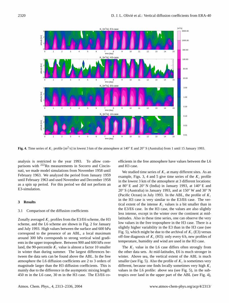
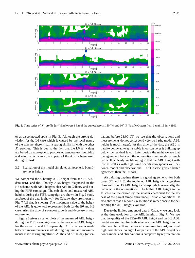
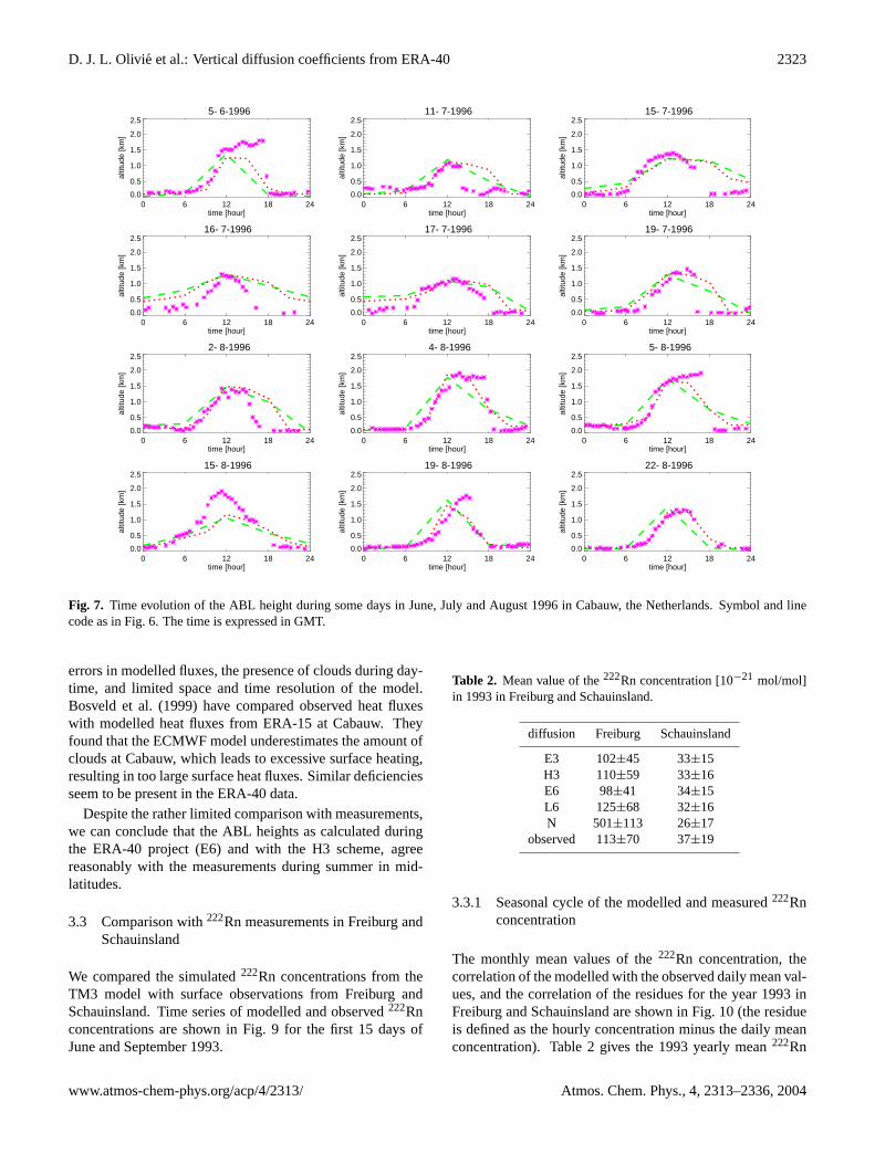
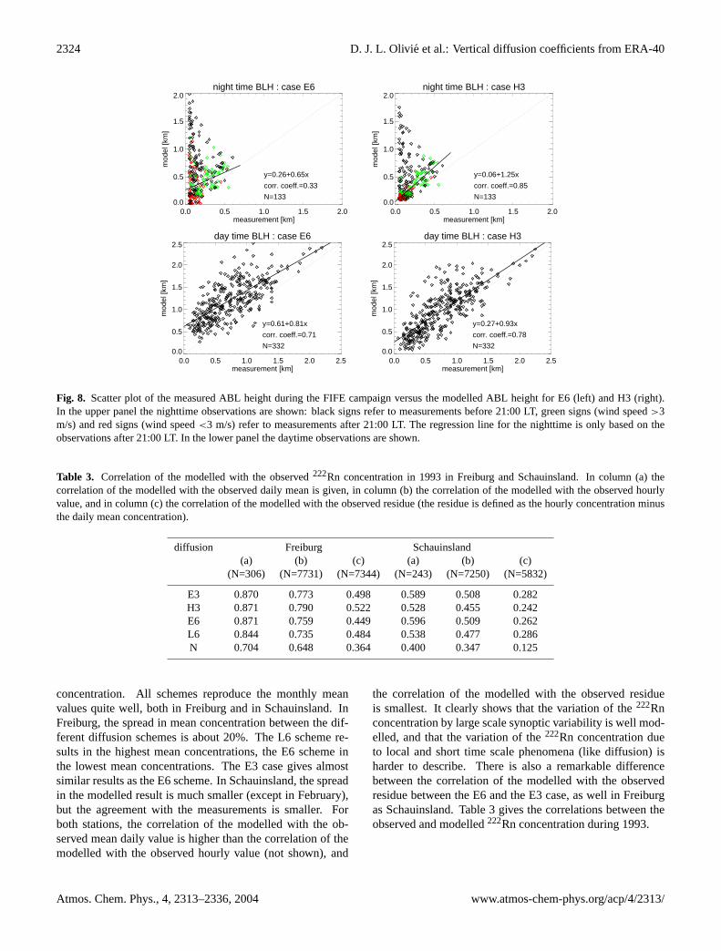
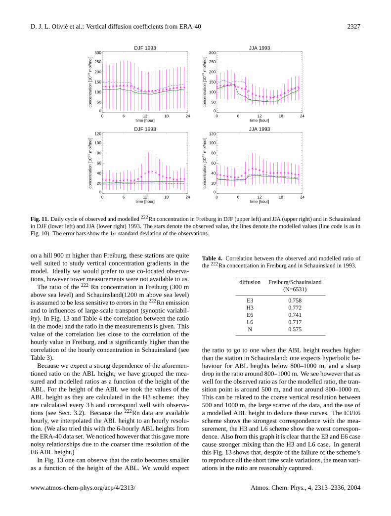