evaluation and development of ... - texas a&m university · pdf filecarlos chang-albitres,...

Technical Report Documentation . Report No.

FHWA/TX-12/0-6386-3

2. Government Accession No.

3. Recipient's Catalog No.

4. Title and Subtitle

EVALUATION AND DEVELOPMENT OF PAVEMENT SCORES, PERFORMANCE MODELS AND NEEDS ESTIMATES FOR THE TXDOT PAVEMENT MANAGEMENT INFORMATION SYSTEM–FINAL REPORT

5. Report Date

Published: October 2012 6. Performing Organization Code

7. Author(s)

Nasir Gharaibeh, Tom Freeman, Siamak Saliminejad, Andrew Wimsatt, Carlos Chang-Albitres, Soheil Nazarian, Imad Abdallah, Jose Weissmann, Angela Jannini Weissmann, Athanassios T. Papagiannakis, and Charles Gurganus

8. Performing Organization Report No.

Report 0-6386-3

9. Performing Organization Name and Address

Texas A&M Transportation Institute The Texas A&M University System College Station, Texas 77843-3135

10. Work Unit No. (TRAIS)

11. Contract or Grant No.

Project 0-6386 12. Sponsoring Agency Name and Address

Texas Department of Transportation Research and Technology Implementation Office P.O. Box 5080 Austin, Texas 78763-5080

13. Type of Report and Period Covered

Technical Report: November 2008–August 201114. Sponsoring Agency Code

15. Supplementary Notes

Project performed in cooperation with the Texas Department of Transportation and the Federal Highway Administration. Project Title: Evaluation and Development of Pavement Scores, Performance Models and Needs Estimates URL: http://tti.tamu.edu/documents/0-6386-3.pdf 16. Abstract

This project conducted a thorough review of the existing Pavement Management Information System (PMIS) database, performance models, needs estimates, utility curves, and scores calculations, as well as a review of District practices concerning the three broad pavement types, asphalt concrete pavement, jointed concrete pavement, and continutously reinforced concrete pavement. The proposed updates to the performance models, utility curves, and decisions trees are intended to improve PMIS scores and needs estimates so that they more accurately reflect District opinions and practices, and reduce performance prediction errors. Reseachers hope that implementation of these PMIS modifications will improve its effectiveness as a decision-aid tool for the Districts. Appendices H, J, and K contain calibrated PMIS performance model coefficients for asphalt concrete pavement (ACP), continuously reinforced concrete pavement (CRCP), and jointed concrete pavement (JCP), respectively; they are recommended for use in the existing PMIS performance models (summarized in Chapter 4). Appendices M and N contain new revised utility curves and coefficients for ACP, CRCP, and JCP pavement distresses. Appendices T, U, and V contain revised ACP, CRCP, and JCP decision trees for needs estimates determination. Appendix Z contains a recommended priority index that can be used for programming projects for preservation, rehabilitation, and reconstruction. 17. Key Words

Pavement Management Information System, PMIS, Asphalt, Concrete, Ride Quality, Performance Model, Utility Curve, Decision Tree

18. Distribution Statement

No restrictions. This document is available to the public through NTIS: National Technical Information Service Alexandria, Virginia http://www.ntis.gov

19. Security Classif. (of this report)

Unclassified

20. Security Classif. (of this page)

Unclassified 21. No. of Pages

302 22. Price

Form DOT F 1700.7 (8-72) Reproduction of completed page authorized

EVALUATION AND DEVELOPMENT OF PAVEMENT SCORES, PERFORMANCE MODELS AND NEEDS ESTIMATES FOR THE TXDOT

PAVEMENT MANAGEMENT INFORMATION SYSTEM–FINAL REPORT

by

Nasir Gharaibeh Assistant Professor

Department of Civil Engineering, Texas A&M University

Tom Freeman

Engineering Research Associate Texas A&M Transportation Institute

Siamak Saliminejad

Graduate Research Assistant Texas A&M Transportation Institute

Andrew Wimsatt

Materials and Pavements Division Head Texas A&M Transportation Institute

Carlos Chang-Albitres

Assistant Professor University of Texas at El Paso

Soheil Nazarian

Professor University of Texas at El Paso

Imad Abdallah

Associate Director, Center for Transportation Infrastructure Systems

University of Texas at El Paso

Jose Weissmann Associate Professor

University of Texas at San Antonio

Angela Jannini Weissmann Transportation Researcher


Athanassios T. Papagiannakis Professor


and

Charles Gurganus Mineola Area Engineer, Tyler District, Texas Department of Transportation

Report 0-6386-3 Project 0-6386

Project Title: Evaluation and Development of Pavement Scores, Performance Models and Needs Estimates

Performed in cooperation with the

Texas Department of Transportation and the

Federal Highway Administration

Published: October 2012

TEXAS A&M TRANSPORTATION INSTITUTE The Texas A&M University System College Station, Texas 77843-3135

v

DISCLAIMER

This research was performed in cooperation with the Texas Department of Transportation (TxDOT) and the Federal Highway Administration (FHWA). The contents of this report reflect the views of the authors, who are responsible for the facts and the accuracy of the data presented herein. The contents do not necessarily reflect the official view or policies of the FHWA or TxDOT. This report does not constitute a standard, specification, or regulation. This report is not intended for construction, bidding, or permit purposes. The engineer in charge of the project was Andrew J. Wimsatt, P.E. #72270 (Texas).

The United States Government and the State of Texas do not endorse products or manufacturers. Trade or manufacturers’ names appear herein solely because they are considered essential to the object of this report.

vi

ACKNOWLEDGMENTS

This project was conducted in cooperation with TxDOT and FHWA. Special thanks go to Bryan Stampley of TxDOT’s Construction Division, project director; Jenny Li, project advisor; and District personnel in Beaumont, Brownwood, Bryan, Dallas, and El Paso who provided ratings of specific sections and project related information. Researchers also thank the other project advisors—Magdy Mikhail, Lisa Lukefahr, Dale Rand, Gary Charlton, Miles Garrison, and Stephen Smith—for their assistance and support, as well as German Claros of TxDOT’s Research and Technology Implementation Office.

vii

TABLE OF CONTENTS

Page List of Figures ................................................................................................................................... x List of Tables ............................................................................................................................... xvii List of Acronyms ............................................................................................................................ xx Chapter 1. Introduction................................................................................................................... 1 Chapter 2. Compare District Rehabilitation and Repair Needs to PMIS Results ..................... 3

Introduction .................................................................................................................................... 3 Methodology .................................................................................................................................. 3 Overview of the PMIS Needs Estimate ......................................................................................... 3 Comparison of Treatments Applied by the District with PMIS Treatment

Recommendations .............................................................................................................. 4 Analysis of Discrepancies in Treatment Selection ...................................................................... 10 Criteria Applied by the Districts for Treatment Selection ........................................................... 15 Budget Prioritization Analysis ..................................................................................................... 15 Conclusions .................................................................................................................................. 20 Recommendations ........................................................................................................................ 21

Chapter 3. District Ratings of Specific Sections and Comparison to PMIS Data .................... 23 Introduction .................................................................................................................................. 23 Section Selection .......................................................................................................................... 23 Data Analysis Summary .............................................................................................................. 23 Conclusions .................................................................................................................................. 34

Chapter 4. Calibration of TxDOT’s Asphalt Concrete Pavement Performance Prediction Models .............................................................................................................. 35

Introduction .................................................................................................................................. 35 Measuring Pavement Performance at TxDOT ............................................................................. 35 Original Pavement Performance Prediction Models ................................................................... 37 Estimation of Pavement Age ....................................................................................................... 39 Evaluation of Original Prediction Models ................................................................................... 41 Data Grouping .............................................................................................................................. 43 Model Calibration Process and Software Tool ............................................................................ 46 Calibrated Models ........................................................................................................................ 49 Assessment of Model Error ......................................................................................................... 77 Summary and Conclusions .......................................................................................................... 78

Chapter 5. Calibration of TxDOT’s Continuously Reinforced Concrete Pavement Performance Prediction Models ....................................................................................... 79

Introduction .................................................................................................................................. 79 Overview of PMIS CRCP Performance Curves .......................................................................... 79 Procedure to Calibrate Pavement Distress Performance Models ................................................ 82 PMIS Data Gathering and Distress Statistical Analysis .............................................................. 83 Conclusions ................................................................................................................................ 119

Chapter 6. Calibration of TxDOT’s Jointed Concrete Pavement Performance Prediction Models ............................................................................................................ 121

Introduction ................................................................................................................................ 121

viii

JCP Distress Types and Evaluation in PMIS ............................................................................. 122 Distress Predictions in PMIS ..................................................................................................... 122 Maintenance and Rehabilitation Treatments in PMIS ............................................................... 123 Methodology .............................................................................................................................. 124 Data Treatment .......................................................................................................................... 125 Updated Models ......................................................................................................................... 130 Summary, Conclusions, and Recommendations ........................................................................ 141

Chapter 7. Proposed Changes to Asphalt Concrete Pavement Utility Curves ...................... 143 Introduction ................................................................................................................................ 143 Alligator Cracking ..................................................................................................................... 144 Patching ..................................................................................................................................... 145 Failures ....................................................................................................................................... 146 Block Cracking .......................................................................................................................... 147 Longitudinal Cracking ............................................................................................................... 148 Transverse Cracks ...................................................................................................................... 149 Raveling and Flushing ............................................................................................................... 150 Percent Sections with Specific Distress ..................................................................................... 151 Proposed Changes to Condition Scores ..................................................................................... 152 Comparisons to Ratings by District Personnel .......................................................................... 156 Summary and Conclusions ........................................................................................................ 174

Chapter 8. Proposed Changes to Continuously Reinforced Concrete Pavement Utility Curves ................................................................................................................... 175

Introduction ................................................................................................................................ 175 Overview of PMIS CRCP Utility Curves .................................................................................. 175 Procedure to Calibrate Pavement Distress Utility Models ........................................................ 180 CRCP Utility Curve Interviews ................................................................................................. 181 Data Compilation and Recalibrations of CRCP Utility Curves ................................................. 182 Conclusions ................................................................................................................................ 185

Chapter 9. Proposed Changes to Jointed Concrete Pavement Utility Curves ....................... 187 Introduction ................................................................................................................................ 187 Interpretation of Utility Equation Coefficients .......................................................................... 188 Objectives of the JCP Utility Curves Update ............................................................................ 190 Methodology for Updating JCP Utilities ................................................................................... 190 Updated Utility Functions .......................................................................................................... 191 PMIS Scores Calculations ......................................................................................................... 210 Impacts, Conclusions, and Recommendations .......................................................................... 210

Chapter 10. Proposed Changes to Asphalt Concrete Pavement Decision Trees .................... 213 Introduction ................................................................................................................................ 213 Deep Rutting Criteria ................................................................................................................. 214 Functional Class Criteria ........................................................................................................... 218 ADT, Distress Quantities, and Ride Quality .............................................................................. 219 PMIS Data Analysis ................................................................................................................... 219 Recommended ACP Decision Tree Trigger Criteria ................................................................. 222

Chapter 11. Proposed Changes to Continuously Reinforced Concrete Pavement Decision Trees .......................................................................................................................... 227

Introduction ............................................................................................................................. 227 Overview of PMIS CRCP Decision Tree ............................................................................... 227

ix

Sensitivity Analysis of Influencing Factors in the Treatment Selection Process ...................... 232 Procedure to Develop a Revised CRCP Decision Tree ............................................................. 235 Revised CRCP Decision Tree .................................................................................................... 236 Conclusions ................................................................................................................................ 239

Chapter 12. Proposed Changes to Jointed Concrete Pavement Decision Trees .................... 241 Introduction ................................................................................................................................ 241 Research Approach .................................................................................................................... 242 Analysis of the PMIS Needs Estimate Tool for JCP ................................................................. 243 Survey of Current District Practices .......................................................................................... 250 JCP Decision Trees Update ....................................................................................................... 255 Impacts, Conclusions, and Recommendations .......................................................................... 261

Chapter 13. Recommendations ................................................................................................... 265 Introduction and Objective ........................................................................................................ 265 Priority Index ............................................................................................................................. 265 Recommended Improvements to the Existing PMIS Components ........................................... 266 Long-Term Recommendations .................................................................................................. 269 Alternative Approaches for the Needs Estimates Tool .............................................................. 271

Incorporating Nondestructive Testing Data in PMIS.................................................................280 References ..................................................................................................................................... 281 Appendices are located on a CD in the back of the report.

x

LIST OF FIGURES

Page Figure 1. Condition Score Comparison, Beaumont District. ........................................................ 24 Figure 2. Distress Score Comparison, Beaumont District. ........................................................... 25 Figure 3. Ride Score Comparison, Beaumont District. ................................................................ 25 Figure 4. Condition Score Comparison, Brownwood District. ..................................................... 26 Figure 5. Distress Score Comparison, Brownwood District. ........................................................ 27 Figure 6. Ride Score Comparison, Brownwood District. ............................................................. 27 Figure 7. Condition Score Comparison, Bryan District. ............................................................... 28 Figure 8. Distress Score Comparison, Bryan District. .................................................................. 29 Figure 9. Ride Score Comparison, Bryan District. ....................................................................... 29 Figure 10. Condition Score Comparison, Dallas. ......................................................................... 30 Figure 11. Distress Score Comparison, Dallas. ............................................................................ 31 Figure 12. Ride Score Comparison, Dallas. .................................................................................. 31 Figure 13. Condition Score Comparison, El Paso. ....................................................................... 32 Figure 14. Distress Score Comparison, El Paso. .......................................................................... 33 Figure 15. Ride Score Comparison, El Paso. ................................................................................ 33 Figure 16. General Shape of Utility Curves Used for Computing DS and CS. ............................ 36 Figure 17. General Shape of TxDOT’s Existing Pavement Performance Prediction

Model. ................................................................................................................................... 38 Figure 18. Illustrative Example 1 of Method Used for Estimating Pavement Age and

Treatment Type. .................................................................................................................... 40 Figure 19. Illustrative Example 2 of Method Used for Estimating Pavement Age and

Treatment Type. .................................................................................................................... 40 Figure 20. Example Actual DS vs. Predicted DS Using PMIS’s Existing Uncalibrated

Model (Pavement Type 4, 5, and 6 with HR in the Beaumont District). ............................. 42 Figure 21. Example Actual DS vs. Predicted DS Using PMIS’s Existing Uncalibrated

Model (Pavement Type 4, 5, and 6 with PM in the Beaumont District). ............................ 42 Figure 22. Performance Pattern Using Original Model Coefficients (Ector County in

Odessa District). .................................................................................................................... 43 Figure 23. Data Grouping for ACP Model Calibration Purposes. ................................................ 44 Figure 24. Climate and Subgrade Zones for ACP Performance Prediction Model

Calibration. ............................................................................................................................ 45 Figure 25. Effect of Model Coefficients on the Li(Age) Curve. ................................................... 47 Figure 26. Genetic Algorithm Used to Solve the Model Calibration Optimization

Problem. ................................................................................................................................ 49 Figure 27. Calibrated and Original DS Prediction Models (Zone 1, Pavement Family A,

& HR). ................................................................................................................................... 51 Figure 28. Calibrated and Original DS Prediction Models (Zone 1, Pavement Family A,

& MR). .................................................................................................................................. 52 Figure 29. Calibrated and Original DS Prediction Models (Zone 1, Pavement Family A,

& LR). ................................................................................................................................... 52 Figure 30. Calibrated and Original DS Prediction Models (Zone 1, Pavement Family A,

& PM). .................................................................................................................................. 53

xi

Figure 31. Calibrated and Original DS Prediction Models (Zone 1, Pavement Family B, & HR). ................................................................................................................................... 53

Figure 32. Calibrated and Original DS Prediction Models (Zone 1, Pavement Family B, & MR). .................................................................................................................................. 54

Figure 33. Calibrated and Original DS Prediction Models (Zone 1, Pavement Family B, & LR). ................................................................................................................................... 54

Figure 34. Calibrated and Original DS Prediction Models (Zone 1, Pavement Family B, & PM). .................................................................................................................................. 55

Figure 35. Calibrated and Original DS Prediction Models (Zone 1, Pavement Family C, & HR). ................................................................................................................................... 55

Figure 36. Calibrated and Original DS Prediction Models (Zone 1, Pavement Family C, & MR). .................................................................................................................................. 56

Figure 37. Calibrated and Original DS Prediction Models (Zone 1, Pavement Family C, & LR). ................................................................................................................................... 56

Figure 38. Calibrated and Original DS Prediction Models (Zone 1, Pavement Family C, & PM). .................................................................................................................................. 57

Figure 39. Calibrated and Original DS Prediction Models (Zone 2, Pavement Family A, & HR). ................................................................................................................................... 57

Figure 40. Calibrated and Original DS Prediction Models (Zone 2, Pavement Family A, & MR). .................................................................................................................................. 58

Figure 41. Calibrated and Original DS Prediction Models (Zone 2, Pavement Family A, & LR). ................................................................................................................................... 58

Figure 42. Calibrated and Original DS Prediction Models (Zone 2, Pavement Family A, & PM). .................................................................................................................................. 59












xii






















Figure 75. Distribution of Standardized Model Error for Both Calibrated and Original Models. .................................................................................................................................. 77

Figure 76. PMIS Performance Curve for Spalled Cracks. ............................................................ 81 Figure 77. PMIS Performance Curve for Punchouts. ................................................................... 81

xiii

Figure 78. PMIS Performance Curve for ACP Patches. ............................................................... 82 Figure 79. PMIS Performance Curve for PCC Patches. ............................................................... 82 Figure 80. Histogram of Observed Li for Spalled Cracks. ............................................................ 84 Figure 81. Relative Frequency Plot of Observed Li for Spalled Cracks. ...................................... 84 Figure 82. Box Plot of Observed Li for Spalled Cracks. .............................................................. 85 Figure 83. Histogram of Li for Punchouts. ................................................................................... 86 Figure 84. Frequency Plot of Li for Punchouts. ............................................................................ 86 Figure 85. Box Plot of Li for Punchouts. ...................................................................................... 87 Figure 86. Histogram of Observed for ACP Patches. ............................................................... 88 Figure 87. Frequency Plot of Observed for ACP Patches. ....................................................... 88 Figure 88. Box Plot of Observed Li for ACP Patches. ................................................................. 89 Figure 89. Histogram of Li for PCC Patches. ............................................................................... 90 Figure 90. Frequency Plot of Li for PCC Patches. ........................................................................ 90 Figure 91. Box Plot of Observed Li for PCC Patches. .................................................................. 91 Figure 92. Histogram for CRCP Distress Scores, Statewide. ....................................................... 93 Figure 93. Relative Frequency Plot for CRCP Distress Score, Statewide. ................................... 93 Figure 94. Box Plot for CRCP Distress Scores, Statewide. .......................................................... 94 Figure 95. Histogram of Li for CRCP Ride Scores. ...................................................................... 95 Figure 96. Relative Frequency Plot of Li for CRCP Ride Scores. ................................................ 95 Figure 97. Box Plot of Li for CRCP Ride Score. .......................................................................... 96 Figure 98. Histogram for CRCP Ride Scores, Statewide. ............................................................ 96 Figure 99. Frequency Plot for CRCP Ride Scores, Statewide. ..................................................... 97 Figure 100. Box Plot for CRCP Ride Scores, Statewide. ............................................................. 97 Figure 101. Histogram for CRCP Condition Scores, Statewide. .................................................. 98 Figure 102. Frequency Plot of CRCP Condition Scores, Statewide. ............................................ 98 Figure 103. Box Plot of Li for CRCP Condition Scores, Statewide. ............................................ 99 Figure 104. Recalibrated CRCP Spalled Cracks Performance Curve, Statewide, Median

Method (Unconstrained). .................................................................................................... 104 Figure 105. Recalibrated CRCP Punchouts Performance Curve, Statewide, Median

Method (Unconstrained). .................................................................................................... 104 Figure 106. Recalibrated CRCP ACP Patches Performance Curve, Statewide, Median

Method (Unconstrained). .................................................................................................... 105 Figure 107. Recalibrated CRCP PCC Patches Performance Curve, Statewide, Median

Method (Unconstrained). .................................................................................................... 105 Figure 108. Recalibrated CRCP Spalled Cracks Performance Curve, Median Method,

(Constrained). ...................................................................................................................... 109 Figure 109. Recalibrated CRCP Punchouts Performance Curve, Median Method,

(Constrained). ...................................................................................................................... 109 Figure 110. Recalibrated CRCP ACP Patches Performance Curve, Median Method,

(Constrained). ...................................................................................................................... 110 Figure 111. Recalibrated CRCP PCC Patches Performance Curve, Median Method,

(Constrained). ...................................................................................................................... 110 Figure 112. Recommended Statewide CRCP Spalled Cracks Performance Curve, Median

Method. ............................................................................................................................... 111 Figure 113. Recommended Statewide CRCP Punchouts Performance Curve, Median

Method. ............................................................................................................................... 112

xiv

Figure 114. Recommended Statewide CRCP ACP Patches Performance Curve, Median Method. ............................................................................................................................... 112

Figure 115. Recommended Statewide CRCP PCC Patches Performance Curve, Median Method. ............................................................................................................................... 113

Figure 116. Recalibrated CRCP Ride Li Performance Curve, Median Method, (Unconstrained). .................................................................................................................. 115

Figure 117. Recalibrated CRCP Ride Li Performance Curve, Median Method, (Constrained). ...................................................................................................................... 116

Figure 118. Climate and Subgrade Zones Utilized for Recalibration of CRCP Performance Curves. ........................................................................................................... 117

Figure 119. Modeling Groups and Grouping Factors. ................................................................ 121 Figure 120. Observed versus Estimated JCP Ages. .................................................................... 128 Figure 121. JCP Distress Progression. ........................................................................................ 128 Figure 122. Failures in Zone 3, Light Rehabilitation. ................................................................. 131 Figure 123. FJC Model for Zones 2 and 3, Light Rehabilitation, Low Traffic. ......................... 132 Figure 124. Failed Joints and Cracks, Zone 1 Models. ............................................................... 132 Figure 125. Failed Joints and Cracks, Zones 2 and 3 Models. ................................................... 133 Figure 126. Failures Models, Zone 1. ......................................................................................... 134 Figure 127. Failures Models, Zone 2. ......................................................................................... 134 Figure 128. Failures Models, Zone 3. ......................................................................................... 135 Figure 129. Concrete Patches Models, Zone 1. .......................................................................... 135 Figure 130. Concrete Patches Models, Zone 2. .......................................................................... 136 Figure 131. Concrete Patches Models, Zone 3. .......................................................................... 136 Figure 132. Longitudinal Cracks Models, Zone 1. ..................................................................... 137 Figure 133. Longitudinal Cracks Models, Zone 2. ..................................................................... 137 Figure 134. Longitudinal Cracks Models, Zone 3. ..................................................................... 138 Figure 135. Shattered Slabs Models. .......................................................................................... 139 Figure 136. Ride Score Frequency Distribution, All Data. ......................................................... 140 Figure 137. Average Ride Score by Treatment and Age. ........................................................... 141 Figure 138. Proposed Alligator Cracking Utility Value. ............................................................ 144 Figure 139. Proposed Patching Utility Value. ............................................................................ 145 Figure 140. Proposed Failure Utility Value. ............................................................................... 146 Figure 141. Proposed Block Cracking Utility Value. ................................................................. 147 Figure 142. Proposed Longitudinal Cracking Utility Value. ...................................................... 148 Figure 143. Proposed Transverse Cracking Utility Value. ......................................................... 149 Figure 144. Proposed Level 2 Flushing and Raveling Utility Value. ......................................... 150 Figure 145. Proposed Level 3 Flushing and Raveling Utility Value. ......................................... 151 Figure 146. PMIS Ride Quality Utility Values. .......................................................................... 153 Figure 147. Proposed Exponents to Ride Utility Function. ........................................................ 155 Figure 148. Proposed Coefficients (Overall) to Ride Utility Function. ...................................... 155 Figure 149. Proposed Coefficients (Ride Score Less than 1) to Ride Utility Function. ............. 156 Figure 150. Distress Scores for Bryan District Sections. ............................................................ 159 Figure 151. Condition Scores for Bryan District Sections. ........................................................ 161 Figure 152. Comparison of District Distress Score for Bryan District to PMIS and

Modified PMIS Score. ........................................................................................................ 161

xv

Figure 153. Comparison of District Condition Score for Bryan District to PMIS and Modified PMIS Score. ........................................................................................................ 162

Figure 154. Distress Scores for Dallas District Sections. ........................................................... 164 Figure 155. Condition Scores for Dallas District Sections. ........................................................ 166 Figure 156. Comparison of District Distress Score for Dallas District to PMIS and

Modified PMIS Score. ........................................................................................................ 166 Figure 157. Comparison of District Condition Score for Dallas District to PMIS and

Modified PMIS Score. ........................................................................................................ 167 Figure 158. Distress Scores for Beaumont District Sections. ..................................................... 168 Figure 159. Condition Scores for Beaumont District Sections. .................................................. 169 Figure 160. Comparison of District Distress Score for Beaumont District to PMIS and

Modified PMIS Score. ........................................................................................................ 170 Figure 161. Comparison of District Condition Score for Beaumont District to PMIS and

Modified PMIS Score. ........................................................................................................ 170 Figure 162. Current PMIS Utility Curve for Spalled Cracks...................................................... 177 Figure 163. Current PMIS Utility Curve for Punchouts. ............................................................ 178 Figure 164. Current PMIS Utility Curve for ACP Patches. ........................................................ 178 Figure 165. Current PMIS Utility Curve for PCC Patches. ........................................................ 179 Figure 166. Current PMIS Utility Curve for Low Traffic Level Ride Quality........................... 179 Figure 167. Current PMIS Utility Curve for Medium Traffic Level Ride Quality. ................... 180 Figure 168. Current PMIS Utility Curve for High Traffic Level Ride Quality. ......................... 180 Figure 169. Recalibrated CRCP Spalled Cracks Utility Curve, Statewide. ............................... 183 Figure 170. Recalibrated CRCP Punchouts Utility Curve, Statewide. ....................................... 183 Figure 171. Recalibrated CRCP ACP Patches Utility Curve, Statewide. ................................... 184 Figure 172. Recalibrated CRCP PCC Patches Utility Curve, Statewide. ................................... 184 Figure 173. Recalibrated CRCP Ride Quality Utility Curve for All Traffic Levels,

Statewide. ............................................................................................................................ 185 Figure 174. Impact of Coefficient α (ρ=β=1). ............................................................................ 189 Figure 175. Impact of Coefficient β. ........................................................................................... 189 Figure 176. Impact of Coefficient ρ. ........................................................................................... 190 Figure 177. Updated Low Traffic Utility Function for Failed Joints and Cracks. ..................... 192 Figure 178. Updated Medium Traffic Utility Function for Failed Joints and Cracks. .............. 193 Figure 179. Updated Heavy Traffic Utility Function for Failed Joints and Cracks. ................. 193 Figure 180. Updated Utility Functions for Failed Joints and Cracks, Comparison. .................. 194 Figure 181. Updated Low Traffic Utility Function for Failures. ................................................ 195 Figure 182. Updated Medium Traffic Utility Function for Failures. .......................................... 195 Figure 183. Updated Heavy Traffic Utility Function for Failures. ............................................. 196 Figure 184. Updated Utility Functions for Failures: Comparison. ............................................. 196 Figure 185. Updated Low Traffic Utility Function for Concrete Patches. ................................. 198 Figure 186. Updated Medium Traffic Utility Function for Concrete Patches. ........................... 198 Figure 187. Updated Heavy Traffic Utility Function for Concrete Patches. .............................. 199 Figure 188. Updated Utility Functions for Concrete Patches: Comparison. .............................. 199 Figure 189. Updated Low Traffic Utility Function for Longitudinal Cracks. ............................ 200 Figure 190. Updated Medium Traffic Utility Function for Longitudinal Cracks. ...................... 201 Figure 191. Updated Heavy Traffic Utility Function for Longitudinal Cracks. ......................... 201 Figure 192. Updated Utility Functions for Longitudinal Cracks: Comparison. ......................... 202

xvi

Figure 193. Updated Low Traffic Utility Function for Shattered Slabs. .................................... 203 Figure 194. Updated Medium Traffic Utility Function for Shattered Slabs. .............................. 203 Figure 195. Updated Heavy Traffic Utility Function for Shattered Slabs. ................................. 204 Figure 196. Updated Utility Functions for Shattered Slabs: Comparison. ................................. 204 Figure 197. Cumulative Ride Score Percentiles in the Historical JCP Database. ...................... 205 Figure 198. Questionnaire Responses and Updated Region of RSL=0. ..................................... 207 Figure 199. Ride Score Loss Utility for Heavy Traffic. ............................................................. 208 Figure 200. Ride Score Loss Utility for Medium and Low Traffic. ........................................... 209 Figure 201. Updated and Original Utility Functions for Ride Score Loss. ................................ 209 Figure 202. Percent of Sections with NN Reason Codes All Pavement Types. ......................... 216 Figure 203. Percent of Sections with NN Reason Codes for Only Asphalt Pavement

Types. .................................................................................................................................. 216 Figure 204. Sections with A705 Reason Code. .......................................................................... 217 Figure 205. Current Deep Rutting Utility Curve from PMIS. .................................................... 218 Figure 206. Functional Classification ADT High/Low Decision Tree. ...................................... 229 Figure 207. CRCP Needs Estimate Decision Tree. .................................................................... 230 Figure 208. Revised Functional Classification ADT High/Low Decision Tree. ........................ 237 Figure 209. Proposed Updates to Current Functional Class/ADT Decision Tree. ..................... 238 Figure 210. Revised CRCP Needs Estimate Decision Tree. ...................................................... 239 Figure 211. Existing Functional Class Decision Tree. ............................................................... 244 Figure 212. Existing JCP Decision Tree. .................................................................................... 248 Figure 213. Updated High Traffic JCP Decision Tree. .............................................................. 258 Figure 214. Updated Low Traffic JCP Decision Tree. ............................................................... 259 Figure 215. Original and Updated Needs Estimates for PMIS 2011. ......................................... 262 Figure 216. Basic Framework for Alternative 1 Needs Estimate Tool. ...................................... 273 Figure 217. Sample Decision Hierarchy. .................................................................................... 277 Figure 218. Sample Distress Hierarchy. ..................................................................................... 279

xvii

LIST OF TABLES

Page Table 1. Factors Used in PMIS to Estimate Needs. ........................................................................ 4 Table 2. PMIS Condition Score, Distress Score, and Ride Score Classes. ..................................... 5 Table 3. Mann-Whitney Test Results for Preventive Maintenance for Beaumont,

Brownwood, Bryan, Dallas, and El Paso Districts in 2007–2009. ......................................... 7 Table 4. Mann-Whitney Test Results for Light Rehabilitation for Beaumont,

Brownwood, Bryan, Dallas, and El Paso Districts in 2007–2009. ......................................... 8 Table 5. Mann-Whitney Test Results for Medium Rehabilitation for Beaumont,

Brownwood, Bryan, Dallas, and El Paso Districts in 2007–2009. ......................................... 9 Table 6. Mann-Whitney Test Results for Heavy Rehabilitation for Beaumont,

Brownwood, Bryan, Dallas, and El Paso Districts in 2007–2009. ....................................... 10 Table 7. Pavement Sections Selected in Brownwood District to Illustrate Discrepancies in

Treatment Selection. ............................................................................................................. 11 Table 8. Flexible Pavement Sections Selected in El Paso District to Illustrate

Discrepancies in Treatment Selection. .................................................................................. 13 Table 9. Concrete Pavement Sections Selected in El Paso District to Illustrate

Discrepancies in Treatment Selection. .................................................................................. 14 Table 10. Sections Selected for Preventive Maintenance, El Paso District (2009). ..................... 17 Table 11. Sections Selected for Rehabilitation, El Paso District (2009). ..................................... 18 Table 12. PMIS Prioritized Sections Not Selected by the District for Treatment in 2009

El Paso District. .................................................................................................................... 19 Table 13. Summary of Treatment Cost and Lane Miles, El Paso District (2009). ....................... 20 Table 14. Original Utility Curve Coefficients ACP. ..................................................................... 37 Table 15. Examples of Treatment Types for ACP. ....................................................................... 39 Table 16. Estimation of DS Thresholds Associated with Different M&R Treatments. ............... 41 Table 17. Counties Used in Model Calibration. ........................................................................... 50 Table 18. Point Sizes Representing the Number of Repeated Data Points in Figures 27–

74. .......................................................................................................................................... 51 Table 19. PMIS Rating for CRCP Distress Types. ....................................................................... 80 Table 20. PMIS Performance Curve Coefficients for CRCP (Type 01). ...................................... 80 Table 21. Li Statistical Parameters for Spalled Cracks. ................................................................ 85 Table 22. Statistical Parameters for ,É for Punchouts. ................................................................. 87 Table 23. ,É Statistical Parameters for ACP Patches. ................................................................... 89 Table 24. LiStatistical Parameters for PCC Patches. ................................................................... 91 Table 25. Number of Sections with Level of Distress (Li) Greater than Zero. ............................. 92 Table 26. Statistical Parameters for CRCP Distress Score, Statewide. ........................................ 94 Table 27. ,ÉStatistical Parameters for CRCP Ride Scores. ......................................................... 95 Table 28. Statistical Parameters for CRCP Ride Scores, Statewide. ............................................ 97 Table 29. ,ÉStatistical Parameters for CRCP Condition Scores, Statewide. ............................... 99 Table 30. Recalibration of CRCP Distress Performance Models. .............................................. 101 Table 31. Recalibration of CRCP Distress Performance Models with Constrained

Parameters. .......................................................................................................................... 106 Table 32. Recommended Statewide CRCP Performance Curve Coefficients. ........................... 112

xviii

Table 33. RSmin Value for Calculating Level of Distress (Li) according to Traffic Category. ............................................................................................................................. 114

Table 34. Recalibration of CRCP Ride (Li) Performance Curves. ............................................. 114 Table 35. Climate and Subgrade Characteristics for Zones. ....................................................... 116 Table 36. Counties in Climate and Subgrade Zones. .................................................................. 117 Table 37. Recalibration of CRCP Performance Curves for Zones. ............................................ 118 Table 38. Recalibration of CRCP Performance Curves for Zones with Constrained

Parameters. .......................................................................................................................... 118 Table 39. JCP Distress Manifestations in PMIS. ........................................................................ 123 Table 40. PMIS Scores Interpretation. ........................................................................................ 123 Table 41. JCP Treatments and Corresponding PMIS Intervention Levels. ................................ 124 Table 42. Summary of Modeling Groups. .................................................................................. 126 Table 43. M&R Treatment Criteria. ........................................................................................... 130 Table 44. Current and Proposed Modified Distress Utility Coefficients. ................................... 143 Table 45. Table of Quantity of Distress at 0, 25, 50, and 90% of Sections with Distress. ......... 151 Table 46. Proposed Exponents and Ride Scores. ........................................................................ 153 Table 47. Distress Score Results from the Bryan District. ......................................................... 157 Table 48. Condition Score Results from the Bryan District. ...................................................... 159 Table 49. Distress Score Results from the Dallas District. ......................................................... 162 Table 50. Condition Score Results from the Dallas District. ...................................................... 164 Table 51. Distress Score Results from the Beaumont District. ................................................... 167 Table 52. Condition Score Results from the Beaumont District. ............................................... 168 Table 53. Summary Statistics for Distress Scores. ..................................................................... 170 Table 54. Summary Statistics for Condition Scores. .................................................................. 170 Table 55. Summary of Distress and Condition Score Ranges. ................................................... 172 Table 56. PMIS Rating for CRCP Distress Types. ..................................................................... 176 Table 57. PMIS Coefficients for CRC Pavements Utility Equations (Type 01). ...................... 177 Table 58. Recalibrated Utility Curve Coefficients for CRCP Distresses and Ride Quality. ..... 182 Table 59. R2 Values for Different Traffic Class Values of Ride Score. ..................................... 185 Table 60. Minimum JCP Ride Score Values. ............................................................................. 187 Table 61. PMIS Scores Interpretation. ........................................................................................ 188 Table 62. Historical Frequencies of Sections by Ride Score Range. .......................................... 206 Table 63. Ride Score Importance to the Condition Score Calculation. ...................................... 210 Table 64. PMIS Needs Estimate Trigger Criteria for Rehabilitation Treatment

Recommendations. .............................................................................................................. 211 Table 65. PMIS Needs Estimate Trigger Criteria for Preventive Maintenance

Recommendations. .............................................................................................................. 212 Table 66. Percent of NN Sections for Bryan, Beaumont, and Dallas. ........................................ 213 Table 67. FY 2011 PMIS–Failures. ............................................................................................ 217 Table 68. FY 2011 PMIS–Alligator Cracking. ........................................................................... 218 Table 69. FY 2011 PMIS–Block Cracking. ................................................................................ 218 Table 70. FY 2011 PMIS–Longitudinal Cracking. ..................................................................... 218 Table 71. FY 2011 PMIS–Distribution of Transverse Cracks. ................................................... 219 Table 72. FY 2011 PMIS–Patching. ........................................................................................... 219 Table 73. FY 2011 PMIS–Deep Rutting. .................................................................................... 219 Table 74. FY 2011 PMIS–Shallow Rutting. ............................................................................... 220

xix

Table 75. Needs Estimate Trigger Criteria for ADT from 0 to 99. ............................................ 220 Table 76. Needs Estimate Trigger Criteria for ADT from 100 to 999. ...................................... 221 Table 77. Needs Estimate Trigger Criteria for ADT from 1000 to 4999. .................................. 221 Table 78. Needs Estimate Trigger Criteria for ADT Greater than or Equal to 5000. ................. 221 Table 79. PMIS Needs Estimate Treatment Levels and Respective Treatment Examples. ....... 225 Table 80. PMIS Functional Classification for Pavement Sections. ............................................ 225 Table 81. CRCP Needs Estimate Tree Input Factor Codes. ....................................................... 229 Table 82. CRCP Needs Estimate Treatment Codes. ................................................................... 229 Table 83. CRCP Needs Estimate Decision Tree Input Factors for the Sensitivity Analysis. ..... 230 Table 84. Statistical Analysis of PMIS CRC Pavement Data, 2011. .......................................... 231 Table 85. Sensitivity Categories for Spearman’s Correlation Coefficient. ................................ 231 Table 86. Sensitivity Analysis Results of Decision Tree Input Factors. .................................... 232 Table 87. Sensitivity Analysis Ranking of Decision Tree Input Factors. ................................... 232 Table 88. Number and Percentage of Lane Miles per Functional Class (CRCP, 2010). ............ 234 Table 89. JCP Treatments and PMIS Intervention Levels. ......................................................... 239 Table 90. JCP Distress Manifestations in PMIS. ........................................................................ 243 Table 91. PMIS 2011 Original Reason Codes and Minimum Treatments for Distress

Thresholds. .......................................................................................................................... 247 Table 92. Surveyed JCP Sections. .............................................................................................. 249 Table 93. Comparison between PMIS and Evaluators’ Recommendations. .............................. 250 Table 94. Survey Recommendations and Their Time Frames. ................................................... 250 Table 95. Averages of Evaluators’ Subjective DS and RS, and of Observed Distress

Levels Triggering Treatment Recommendations (Next-Year Equivalency). ..................... 251 Table 96. Individual Distress Values Required to Reach DS Levels. ........................................ 252 Table 97. Updated Reason Codes and Frequency of PMIS 2011 Sections. ............................... 255 Table 98. ESALs and Functional Class Traffic Levels. .............................................................. 259 Table 99. Original and Updated Needs Estimates for PMIS 2011. ............................................ 261 Table 100. Needs Estimates Comparison by Section Condition. ............................................... 262 Table 101. Decision Matrix Definitions and Explanations. ........................................................ 275 Table 102. Example Completed Matrix. ..................................................................................... 276 Table 103. Example Importance Levels. .................................................................................... 278

xx

LIST OF ACRONYMS

AADT Average Annual Daily Traffic ACP Asphalt Concrete Pavement ACS Average crack spacing ADT Average daily traffic AHP Analytic Hierarchy Process AJS Apparent joint spacing CRCP Continuously Reinforced Concrete Pavement CP Concrete patches CPR Concrete pavement restoration CRF Average country rainfall CS Condition score CSJ Control Section Job (TxDOT Construction Project Designation) DS Distress score DV Decision variable ESAL Equivalent Single Axle Load FC Functional class FJC Failed joints and cracks FL Failures FPS19 Texas Flexible Pavement Design System GA Genetic algorithm HR Heavy rehabilition IRI Ride Quality JCP Jointed Concrete Pavement LC Longitudinal cracks Li Level of distress LR Light rehabilitation M&R Maintenance and rehabilitation MR Medium rehabilitation NN Needs nothing PCC Portland Cement Concrete PM Preventive maintenance PMIS Pavement Management Information System RV Real value RS Ride score RSL Ride score loss RSME Root Mean Squared Error SS Shattered slabs TxDOT Texas Department of Transportation α Maximum loss factor β Slope factor ρ Prolongation factor

1

CHAPTER 1. INTRODUCTION

This report documents comparisons, calibration of pavement performance models, proposed changes to utility curves, and proposed changes to decision trees conducted under the project titled, Evaluation and Development of Pavement Scores, Performance Models and Needs Estimates. The project was split into three phases. Phase I involves a review of the current Pavement Management Information System (PMIS) and recommendations for modifying and improving analytical processes in the system. Phase II involves developing pavement performance models for the system. Finally, Phase III involves developing improved decision trees for the system’s needs estimate process.

The first project task involved developing a synthesis on how states define and measure pavement scores; that synthesis was published in report 0-6386-1 in February 2009.

The second report, published as 0-6386-2, contains the results of a literature review relating to this research; a review of the current PMIS score process and recommendations based on that review; and preliminary conclusions. The report also contains a summary of interviews with Texas Department of Transportation (TxDOT) personnel concerning distresses collected and stored in PMIS; sample pavement performance indices from Pennsylvania, Ohio, Oregon, and South Dakota; and a sensitivity analysis of the PMIS score process.

This report documents the remaining work conducted in this study. The following chapters and in this report:

Chapter 2 documents the comparison between District Priority Ranking and Repair Needs to PMIS results.

Chapter 3 documents TxDOT District ratings of specific sections and comparison to the PMIS data.

Chapter 4 documents the calibration of the PMIS Asphalt Concrete Pavement (ACP) Performance Prediction Models.

Chapter 5 documents the calibration of the PMIS Continuously Reinforced Concrete Pavement (CRCP) Performance Prediction Models in PMIS.

Chapter 6 documents the calibration of the PMIS Jointed Concrete Pavement (JCP) Performance Prediction Models in PMIS.

Chapter 7 documents proposed changes to Asphalt Concrete Pavement Utility Curves. Chapter 8 documents proposed changes to CRCP Utility Curves. Chapter 9 documents proposed changes to JCP Utility Curves. Chapter 10 documents proposed changes to ACP Decision Tree Trigger Criteria. Chapter 11 documents proposed changes to CRCP Decision Tree Trigger Criteria. Chapter 12 documents proposed changes to JCP Decision Tree Trigger Criteria. Chapter 13 contains conclusions and recommendations.

The report also contains 26 technical appendices (Appendices A through Z) that document specific details of the study. The following major appendices that were required by TxDOT are as follows. Appendices H, J, and K contain calibrated PMIS performance model coefficients for asphalt concrete pavement (ACP), continuously reinforced concrete pavement (CRCP), and

2

jointed concrete pavement (JCP), respectively; they are recommended for use in the existing PMIS performance models (summarized in Chapter 4). Appendices M and N contain new revised utility curves and coefficients for ACP, CRCP, and JCP pavement distresses. Appendices T, U, and V contain revised ACP, CRCP, and JCP decision trees for needs estimates determination. Appendix Z contains a recommended priority index that can be used for programming projects for preservation, rehabilitation, and reconstruction.

3

CHAPTER 2. COMPARE DISTRICT REHABILITATION AND REPAIR NEEDS TO PMIS RESULTS

INTRODUCTION

This chapter documents a comparison of rehabilitation and repair needs provided by experienced District personnel with those provided by PMIS. Beaumont, Brownwood, Bryan, Dallas, and El Paso Districts were selected for the purpose of this analysis because of their range of pavement types, environmental conditions, traffic levels, and pavement ages in their regions.

METHODOLOGY

Researchers met with District personnel to obtain a list of preventive maintenance and rehabilitation treatments applied by the District and compare them to PMIS scores and treatment needs recommendations. Treatments applied by the District from 2007 through 2009 were collected for the purpose of this analysis. The amount and level of detail of historical information available about treatments applied by each District vary and the type of analysis conducted during this task was coordinated with each District. The overall methodology followed to perform this subtask is summarized as follows:

Visit the District to obtain a historical list of preventive maintenance and rehabilitation

treatments. Treatments applied by the District were collected at least from 2007 through 2009.

Conduct statistical analysis with PMIS data including Condition Scores, Distress Scores, treatments recommended by PMIS. PMIS data from 2001 through 2009 were analyzed for each District.

Conduct a comparison between PMIS data and information provided by the Districts. This comparison was conducted for treatments applied from 2007 through 2009.

Summarize analysis and findings from the comparison and provide overall recommendations.

OVERVIEW OF THE PMIS NEEDS ESTIMATE

PMIS estimates needs in terms of dollars and lane miles of pavement sections recommended for preventive maintenance and rehabilitation. The following treatment categories are defined in PMIS:

Needs Nothing (NN). Preventive Maintenance (PM). Light Rehabilitation (LR). Medium Rehabilitation (MR). Heavy Rehabilitation or Reconstruction (HR).

4

PMIS selects the appropriate treatments using an “if-then” decision tree with trigger criteria based on “reason codes” associated to each treatment category. The “reason code” provides the District engineer with a clue of the factors that prompted the treatment recommendation. Factors used in PMIS to estimate needs are listed in Table 1.

Table 1. Factors Used in PMIS to Estimate Needs. …Factor Used For

Pavement Type Decision tree statements (ACP, CRCP, or JCP) Distress Scores Decision tree statements Ride Score Decision tree statements (rehab treatments only) Average Daily Traffic (ADT)

Decision tree statements (ADT per lane)

Number of Lanes Decision tree statements (ADT per lane) and to compute treatment cost in terms of lane miles

Functional Class Decision tree statements (used with ADT per lane)

County Decision tree statements (heavy rehab on CRCP) and to compute pavement needs in future years

Date of Last Surface Decision tree statements (preventive maintenance seal coats) 18-k ESAL Computing pavement needs in future years Section Length Computing treatment cost in terms of lane miles The PMIS Condition Scores are not directly related to the treatment selection. As a result, it is possible for a pavement section with a high Condition Score to receive a treatment heavier than a section with a low Condition Score. It is also possible that PMIS recommends PM or NN for sections with Condition Scores below 70.

COMPARISON OF TREATMENTS APPLIED BY THE DISTRICT WITH PMIS TREATMENT RECOMMENDATIONS

The study included the statistical analysis of the PMIS data only and a comparison of treatments applied by the District with PMIS treatment recommendations. Details about the analysis conducted for each District are in the appendices. The appendices include:

Summary of PMIS Scores (Appendix A): Appendix A includes a summary of the results for all the five Districts. Each District’s lane miles and percentages grouped by Condition Score, Distress Score, and Ride Score classes are reported and compared to the statewide statistics. The annual average scores for each District compared to the statewide scores are also included. The PMIS data from fiscal years 2001 through 2009 were used for this comparison. Table 2 shows PMIS score classes.

5

Table 2. PMIS Condition Score, Distress Score, and Ride Score Classes. Classification Condition Score Distress Score Ride Score

Very Good 90–100 90–100 4.0–5.0 Good 70–89 80–89 3.0–3.9 Fair 50–69 70–79 2.0–2.9 Poor 35–49 60–69 1.0–1.9

Very Poor 1–34 1–59 0.1–0.9

PMIS Treatment Needs and Scores by Treatment Category (Appendix B): Total lane miles by PMIS treatment category are shown from fiscal years 2001 through 2009. Summaries are provided for all pavement types, asphalt, and concrete. Minimum, maximum, mean, standard deviation, and quartiles of PMIS scores by PMIS treatment category are reported from 2001 through 2009. PMIS treatment categories include: NN, PM, LR, MR, and HR. Analyses were performed for all types of rigid and flexible pavements.

Comparison of PMIS Scores for Treatments Applied in the District with PMIS Treatment Recommendations (Appendix C): PMIS scores for pavement sections that received treatment from 2007 through 2009 are included in this appendix. Minimum, maximum, mean, standard deviation, and quartiles of PMIS scores by PMIS treatment category for pavement sections that received treatment from 2007 through 2009 are included in that appendix.

Evolution of PMIS Scores due to Treatments Applied by the District (Appendix D): A comparison of PMIS scores before and after treatment is reported including the frequency (number of sections) and cumulative frequency. Analyses were conducted for District sections that received treatments in years 2007, 2008, and 2009.

Answers from the Districts to Questionnaires about Treatment Selection Philosophy (Appendix E): Interviews were conducted with District personnel to document how the District currently selects road for a construction project and then decide what treatment category to apply. Variables, in order of priority, affecting their decision on what road sections will receive treatment and what type of work will be performed are also documented.

Budget Prioritization Analyzes and PMIS Ranking for Sections Selected by the District for Treatment (Appendix F): A sufficient budget prioritization analysis was used to determine differences in philosophy for sections selected for treatment by the District when compared to PMIS recommendations.

Statistical Tests to Compare PMIS Treatment Recommendations with Treatments Applied in the Beaumont, Brownwood, Bryan, Dallas, and El Paso Districts

Hypothesis tests were performed to compare if the scores for the PMIS treatment recommendations were statistically different than the scores for treatments applied by the District. A preliminary analysis of the score histograms by treatment category shows that they do not follow a normal distribution. Therefore, nonparametric statistical tests were selected to perform the analysis.

Nonparametric tests are not completely free of assumptions about the data since they still require the data to be independent random samples. The Mann-Whitney nonparametric hypothesis test

6

was used to determine whether the medians () of the PMIS scores were statistically different for PMIS treatment recommendations when compared to treatments applied by the District. The Mann-Whitney test does not require the data to come from normally distributed populations, but it does make the following assumptions: (a) the histograms and the distribution curves of the scores for the PMIS treatment recommendations and treatments applied by the District show the similarity in shapes, and (b) all the scores from PMIS treatment recommendations and treatments applied by the District are independent of each other. In probability theory, the two events are independent, which intuitively means that the occurrence of one event makes it neither more nor less probable that the other occurs.

The test is formulated as follow:

Null hypothesis -> H0: = (medians are equal). Alternative hypothesis -> Ha: ≠ (medians are not equal).

The Mann-Whitney test uses the ranks of the sample data, instead of their specific values, to detect statistical significance. The test was performed at the 0.05 significance level. If the test’s p-value is less than 0.05 then we reject the null hypothesis.

Tables 3–6 show the results of the two samples’ Mann-Whitney hypothesis testing when comparing scores for PMIS treatment recommendations and treatments applied by Beaumont, Brownwood, Bryan, Dallas, and El Paso Districts. Analysis was conducted from 2007 to 2009 for PM, LR, MR, and HR. We should expect the PMIS score statistics for each treatment category to be statistically equal when compared to District score statistics for treatments applied. This expectation should be reflected in the results of the Mann-Whitney test by accepting the null hypothesis of equal medians, which means that PMIS and District score statistics belong to the same population.

The bottom of each table has a summary of PMIS and District records relating to the table results. For example, at the bottom of table 3, “3682-1602 Beaumont” indicates that 3,682 PMIS sections are recommended for preventive maintenance according to PMIS. However, 1,602 PMIS sections received preventive maintenance treatments according to Beaumont District records.

For PM, results of the Mann-Whitney tests show statistical differences for the PMIS Condition Score, Distress Score, and Ride Score medians when comparing PMIS recommendations to treatments applied in Beaumont, Bryan, and El Paso Districts. However for Brownwood District the null hypothesis should be accepted for Condition, Distress, and Ride Scores. For Dallas, we should accept the null hypothesis of equal means for the Condition Score and reject it for distress and Ride Score.

7

Table 3. Mann-Whitney Test Results for Preventive Maintenance for Beaumont, Brownwood, Bryan, Dallas, and El Paso Districts in 2007–2009.

PMIS- District records: 3682-1602 Beaumont, 8473-1208 Brownwood, 5225-1485 Bryan, 8012-1716 Dallas, 3057-267 El Paso.

Year Score Medians

P-Value

Test Result PMIS District

Beaumont Condition Score 90 100 0.0000 Reject Distress Score 91 100 0.0000 Reject

Ride Score 3.4 3.6 0.000 Reject

Brownwood

Condition Score 99 100 0.1024 Accept

Distress Score 100 100 0.2650 Accept

Ride Score 3.3 3.4 0.7428 Accept

Bryan

Condition Score 90 95 0.0000 Reject

Distress Score 92 97 0.0000 Reject


Dallas




El Paso




8

Table 4. Mann-Whitney Test Results for Light Rehabilitation for Beaumont, Brownwood, Bryan, Dallas, and El Paso Districts in 2007–2009.

PMIS- District records: 552-213Beaumont, 749-27 Brownwood, 1834-36 Bryan, 2860-267 Dallas, 0-0 El Paso. For the LR, results of the Mann-Whitney tests show a statistical difference for PMIS Condition Score, Distress Score, and Ride Score medians when comparing PMIS recommendations to treatments applied in Beaumont, and Dallas Districts. In the Brownwood District the null hypothesis of equal means should be accepted for condition and Distress Scores while rejected for Ride Score. In Bryan, the null hypothesis of equal means should be accepted for Distress Score and rejected for condition and Ride Scores. No light rehabilitation treatments were applied in the El Paso District from 2007–2009.

For MR, results of the Mann-Whitney tests show a statistical difference for PMIS Condition Score, Distress Score, and Ride Score medians when comparing PMIS recommendations to treatments applied in Bryan District. In Beaumont, Brownwood, and Dallas the null hypothesis of equal means should be accepted for Distress Score and rejected for condition and Ride Scores. No MR treatments were applied in the El Paso District from 2007–2009.

For HR, results of the Mann-Whitney tests show statistical differences for PMIS Condition Score, Distress Score, and Ride Score medians when comparing PMIS recommendations to treatments applied in Beaumont, Brownwood, and Dallas Districts. In the Bryan District the null hypothesis of equal means should be accepted for the Distress Score and rejected for condition and Ride Scores. No HR treatments were applied in the El Paso District from 2007–2009.

Year Score Medians

P-Value


Beaumont




Brownwood




Bryan




Dallas




El Paso

Condition Score - - - -

Distress Score - - - -

Ride Score - - - -

9

Table 5. Mann-Whitney Test Results for Medium Rehabilitation for Beaumont, Brownwood, Bryan, Dallas, and El Paso Districts in 2007–2009.


Year Score Medians

P-Value


Beaumont




Brownwood




Bryan




Dallas




El Paso



Ride Score - - - -

10

Table 6. Mann-Whitney Test Results for Heavy Rehabilitation for Beaumont, Brownwood, Bryan, Dallas, and El Paso Districts in 2007–2009.


ANALYSIS OF DISCREPANCIES IN TREATMENT SELECTION

Individual pavement sections with discrepancies between the treatments recommended by the PMIS and the treatments applied were analyzed with District personnel. Table 7 shows a summary of pavement sections selected to illustrate discrepancies in treatment selection in Brownwood District. Tables 8 and 9 show a summary of the asphalt and concrete sections selected to illustrate discrepancies in treatment selection in the El Paso District.

Criteria used to select these sections included functional class, level of traffic, pavement type, and PMIS scores. Pavement sections with high Condition Score and low Ride Score or low Condition Score but high Ride Score also were considered when selecting these sections. It is observed that in addition to PMIS scores, engineering judgment regarding the importance of the road section, location, traffic level, and budget constraints influence the final decision when selecting a treatment.

Year Score Medians

P-Value


Beaumont




Brownwood




Bryan




Dallas




El Paso



Ride Score - - - -

Tab

le 7

. Pav

emen

t Sec

tions

Sel

ecte

d in

Bro

wnw

ood

Dis

tric

t to

Illus

trat

e D

iscr

epan

cies

in T

reat

men

t Sel

ectio

n.

PMIS

B

RO

WN

WO

OD

DIS

TR

ICT

FISC

AL

Y

EA

R

SIG

NE

D

HIG

HW

AY

B

RM

E

RM

A

AD

T

CU

RR

EN

T

TR

UC

K A

AD

T

PCT

CU

M A

DT

O

RIG

SU

RFA

CE

Q

TY

CO

ND

ITIO

N

SCO

RE

R

IDE

SC

OR

E

DIS

TR

ESS

SC

OR

E

TR

EA

TM

EN

T

AB

BR

EV

.

TR

EA

TM

EN

T

App

lied

by th

e D

istr

ict

Dis

tric

t Rea

son

2007

FM

1030

03

78 +

01.0

03

78 +

01.5

16

0 46

.8

9052

00

19

2.1

20

MR

PM

Lo

w A

DT,

Rur

al, N

ot H

igh

Prio

rity,

Se

al C

oat.

2007

FM

1030

03

78 +

00.0

03

78 +

00.5

24

0 37

.3

1949

100

23

1.9

28

MR

PM

20

07

FM10

30

0376

+01

.5

0378

+00

.0

240

37.3

19

4910

0 46

1.

8 59

M

R

PM

2007

FM

1030

03

78 +

00.5

03

78 +

01.0

16

0 46

.8

9052

00

55

2.3

55

LR

PM

2008

FM

1176

03

48 -0

0.2

0348

+00

.0

910

4.6

5179

350

58

1.9

69

MR

PM

N

ear r

ailro

ad th

eref

ore

caus

ing

ride

to b

e lo

w. I

n ho

use

forc

es w

ill

mai

ntai

n.

Low

AD

T, S

eal C

oat.

2008

FM

1176

03

48 +

00.5

03

48 +

01.0

19

0 8.

6 14

5635

0 77

1.

8 10

0 M

R

PM

2008

FM

1176

03

48 +

01.5

03

50 +

00.0

19

0 8.

6 14

5635

0 99

2.

2 10

0 LR

PM

20

08

FM11

76

0348

+00

.0

0348

+00

.5

910

4.6

6000

600

75

2.4

90

LR

PM

2008

FM

1770

04

22 +

01.5

04

22 +

01.7

38

0 29

.4

2361

550

48

2.2

49

LR

PM

Low

AD

T, R

ural

, Not

Hig

h Pr

iorit

y,

Seal

Coa

t. 20

08

FM17

70

0422

+00

.5

0422

+01

.0

270

35

1357

800

78

2.4

78

LR

PM

2008

FM

1770

04

22 +

01.0

04

22 +

01.5

38

0 29

.4

2565

950

95

2.1

100

LR

PM

2008

FM

2302

03

28 +

01.0

03

28 +

01.5

11

0 10

62

7800

83

2.

3 83

LR

PM

Lo

w A

DT,

Rur

al, N

ot H

igh

Prio

rity,

Se

al C

oat.

2008

FM

2302

03

28 +

01.5

03

30 +

00.0

11

0 10

62

7800

96

2.

3 96

LR

PM

2008

FM

3099

02

64 +

01.0

02

64 +

01.5

10

50

18.9

76

1755

0 52

2.

4 62

LR

PM

H

ad a

lot o

f spo

t rep

air p

rior t

o se

al

coat

and

that

is w

hy th

e sc

ore

was

lo

w. S

truct

ure

is ok

. 20

08

FM30

99

0266

+01

.6

0266

+02

.1

1050

18

.9

5967

750

61

2.3

78

LR

PM

2008

FM

0567

03

44 +

00.5

03

44 +

01.0

70

8.

9 57

3050

85

2.

4 85

LR

PM

Lo

w A

DT,

Rur

al, N

ot H

igh

Prio

rity,

Se

al C

oat.

2008

FM

0567

03

44 +

00.0

03

44 +

00.5

70

8.

9 58

0350

90

2

100

LR

PM

2008

FM

0567

03

42 +

01.0

03

42 +

01.5

70

8.

9 58

0350

98

2.

4 98

LR

PM

20

08

FM05

67

0342

+01

.5

0344

+00

.0

70

8.9

5803

50

100

2.4

100

LR

PM

2008

FM

0569

03

00 +

01.5

03

02 +

00.0

11

0 8.

2 52

9250

96

2.

4 96

LR

PM

Low

AD

T, R

ural

, Not

Hig

h Pr

iorit

y,

Seal

Coa

t.

2008

FM

0588

03

20 +

01.0

03

20 +

01.5

21

0 6.

2 10

7310

0 66

2.

1 69

LR

PM

20

08

FM05

88

0322

+00

.0

0322

+00

.5

210

6.2

1073

100

100

2.4

100

LR

PM

2008

FM

0589

04

76 +

00.5

04

76 +

01.0

12

0 8.

4 83

9500

95

2.

1 10

0 LR

PM

20

08

FM05

89

0474

+01

.0

0474

+01

.5

120

8.4

8395

00

100

2.3

100

LR

PM

2008

FM

0701

02

70 +

00.5

02

70 +

00.7

17

0 26

.8

1164

350

73

2.2

74

LR

PM

2008

FM

0701

02

62 +

00.5

02

62 +

01.0

15

0 27

.9

9599

50

88

2.3

88

LR

PM

2009

IH

0020

03

63 +

00.0

03

63 +

00.1

88

50

41.4

50

8372

00

10

3.4

10

MR

H

R

361-

364

Som

e se

ctio

ns w

ere

very

ba

d w

ith lo

w d

istre

ss sc

ore

so w

e di

d a

reco

nstru

ct. I

t had

failu

re a

nd

fatig

ue c

rack

ing.

We

rem

oved

H

MA

, rew

orke

d ba

se, a

nd a

dded

15"

H

MA

. Exi

stin

g st

ruct

ure

was

not

ad

equa

te fo

r tra

ffic.

2009

IH

0020

03

63 +

00.1

03

63 +

00.6

88

50

41.4

50

8372

00

12

2.9

14

MR

H

R

2009

IH

0020

03

61 +

00.0

03

61 +

00.6

88

40

41.4

49

9009

75

20

3.8

20

MR

H

R

2009

IH

0020

03

63 +

00.6

03

63 +

00.9

88

50

41.4

50

8372

00

24

3.3

24

MR

H

R

2009

IH

0020

03

62 +

00.0

03

62 +

00.2

88

50

41.4

50

8372

00

26

4.1

26

MR

H

R

2009

IH

0020

03

62 +

00.4

03

63 +

00.0

88

50

41.4

50

8372

00

26

3.4

26

MR

H

R

2009

IH

0020

03

63 +

00.6

03

63 +

00.9

88

50

41.4

50

8372

00

36

3.4

36

MR

H

R

2009

IH

0020

03

63 +

00.1

03

63 +

00.6

88

50

41.4

50

8372

00

46

3.8

46

PM

HR

2

Tab

le 7

. Pav

emen

t Se

ctio

ns S

elec

ted

in B

row

nwoo

d D

istr

ict

to I

llus

trat

e D

iscr

epan

cies

in T

reat

men

t S

elec

tion

(C

onti

nue

d).

P

MIS

B

RO

WN

WO

OD

DIS

TR

ICT

FIS

CA

L

YE

AR

S

IGN

ED

H

IGH

WA

Y

BR

M

ER

M

AA

DT

C

UR

RE

NT

T

RU

CK

AA

DT

P

CT

CU

M A

DT

O

RIG

SU

RF

AC

E

QT

Y

CO

ND

ITIO

N

SC

OR

E

RID

E

SC

OR

E

DIS

TR

ES

S

SC

OR

E

TR

EA

TM

EN

T

AB

BR

EV

.

TR

EA

TM

EN

T

Ap

pli

ed b

y th

e D

istr

ict

Dis

tric

t R

easo

n

2009

IH

0020

03

62 +

00.2

03

62 +

00.4

88

50

41.4

50

8372

00

55

3.2

56

MR

H

R

361-

364

Som

e se

ctio

ns w

ere

very

ba

d w

ith

low

dis

tres

s sc

ore

so w

e di

d a

reco

nstr

uct.

It h

ad f

ailu

re a

nd

fati

gue

crac

king

. We

rem

oved

HM

A,

rew

orke

d ba

se, a

nd a

dded

15"

HM

A.

Exi

stin

g st

ruct

ure

was

not

ade

quat

e fo

r tr

affi

c.

2009

IH

0020

03

61 +

00.6

03

62 +

00.0

88

50

41.4

50

8372

00

67

4.1

67

PM

HR

20

09

IH00

20

0363

+00

.0

0363

+00

.1

8850

41

.4

5083

7200

74

4.

1 74

PM

H

R

2009

IH

0020

03

62 +

00.2

03

62 +

00.4

88

50

41.4

50

8372

00

82

4 82

PM

H

R

2009

IH

0020

03

60 +

00.6

03

61 +

00.0

88

40

41.4

49

8900

25

86

3.6

86

PM

HR

20

09

IH00

20

0361

+00

.6

0362

+00

.0

8850

41

.4

5083

7200

89

4.

1 89

PM

H

R

2009

IH

0020

03

61 +

00.0

03

61 +

00.6

88

40

41.4

49

9009

75

91

3.9

91

PM

HR

20

09

IH00

20

0362

+00

.0

0362

+00

.2

8850

41

.4

5083

7200

93

4

93

PM

HR

20

09

IH00

20

0360

+00

.0

0360

+00

.6

8840

41

.4

4989

0025

94

3.

3 94

PM

H

R

2009

IH

0020

03

62 +

00.4

03

63 +

00.0

88

50

41.4

50

8372

00

96

3.9

96

PM

HR

2009

IH

0020

03

60 +

00.6

03

61 +

00.0

88

40

41.4

49

8900

25

99

3.5

99

PM

HR

T

his

was

a P

M. W

e m

ille

d an

d ov

erla

yed

wit

h 2"

of

hot m

ix. T

here

w

ere

som

e fa

ilur

es, r

uts

and

fati

gue

crac

king

. Fai

lure

s an

d fa

tigue

cr

acki

ng w

ere

repa

ired

pri

or to

ov

erla

y.

2009

IH

0020

03

60 +

00.0

03

60 +

00.6

88

40

41.4

49

8900

25

99

3.2

100

PM

HR

2007

SH

0016

03

42 -

01.4

03

42 -

01.0

69

20

12.7

45

3403

00

45

2.4

84

MR

PM

We

did

leve

l up

and

appl

ied

a se

al

coat

.

2007

SH

0016

03

56 +

00.5

03

56 +

01.0

61

40

13

3534

6600

64

2.

6 99

L

R

PM

2007

SH

0016

04

14 +

00.0

04

14 +

00.5

30

00

17.7

18

3595

00

49

2.4

59

MR

PM

20

07

SH00

16

0388

+01

.0

0388

+01

.3

1300

20

68

2550

0 32

3.

8 32

M

R

PM

2007

SH

0016

03

40 +

00.0

03

40 +

00.1

15

50

18.6

11

3515

00

78

2.3

100

MR

PM

2008

U

S018

0 04

74 +

01.5

04

76 +

00.0

95

00

33.1

59

9658

50

46

2.3

96

MR

PM

B

ad r

ide.

Lev

el u

p an

d se

al c

oat.

2008

U

S018

3 03

00 +

00.5

03

00 +

01.0

62

00

13.6

33

9158

00

29

2.6

44

MR

PM

R

epai

r fa

ilur

es, f

ill in

rut

s, a

nd s

eal

coat

. 20

09

US0

067

0574

+01

.5

0576

+00

.0

5500

11

.4

0 53

3

59

PM

PM

Thi

s w

as a

PM

job

wit

h 2"

mil

l and

ov

erla

y. L

ocal

ized

rep

airs

wer

e m

ade

prio

r to

sea

l coa

t.

2009

U

S006

7 05

74 +

00.5

05

74 +

01.0

55

00

11.4

0

64

3.1

67

PM

PM

2009

U

S006

7 05

74 +

00.5

05

74 +

01.0

55

00

11.4

0

65

3.8

65

PM

PM

2009

U

S006

7 05

76 +

00.0

05

76 +

00.5

55

00

11.4

0

67

3.5

67

PM

PM

2009

U

S006

7 05

74 +

01.5

05

76 +

00.0

55

00

11.4

0

74

3.2

75

PM

PM

2009

U

S006

7 05

74 +

01.0

05

74 +

01.5

55

00

11.4

0

74

3.4

74

PM

PM

2009

U

S006

7 05

76 +

00.0

05

76 +

00.5

55

00

11.4

0

81

3.6

81

PM

PM

2009

U

S006

7 05

74 +

01.0

05

74 +

01.5

55

00

11.4

0

90

3.2

91

PM

PM

2009

U

S006

7 05

72 +

01.2

05

74 +

00.0

55

00

11.4

0

92

3.8

92

PM

PM

2009

U

S006

7 05

72 +

01.2

05

74 +

00.0

55

00

11.4

0

96

3.8

96

PM

PM

Thi

s is

a r

econ

stru

ctio

n. R

ewor

k ex

isti

ng p

avem

ent,

add

new

fle

xibl

e ba

se a

nd 2

CS

T. T

he s

ectio

n w

as

seal

ed r

ecen

tly

to h

old

toge

ther

. It i

s ha

rd to

see

the

dist

ress

and

ther

efor

e th

e st

ruct

ure

was

wor

se th

an it

sh

ows.

2009

U

S008

4 05

98 +

01.0

05

98 +

01.5

22

00

26.5

0

52

3.3

52

PM

LR

2009

U

S008

4 06

00 +

00.5

06

00 +

01.0

22

00

26.5

0

54

3.4

54

MR

L

R

2009

U

S008

4 06

00 +

01.5

06

02 +

00.0

19

50

25.6

0

54

3.4

54

MR

L

R

2009

U

S008

4 06

00 +

00.0

06

00 +

00.5

22

00

26.5

0

88

2.7

90

PM

LR

1

Tab

le 8

. Fle

xib

le P

avem

ent

Sec

tion

s S

elec

ted

in E

l Pas

o D

istr

ict

to I

llu

stra

te D

iscr

epan

cies

in T

reat

men

t S

elec

tion

.

PM

IS

El P

aso

Dis

tric

t

FIS

CA

L

YE

AR

SIG

NE

D

HIG

HW

AY

ID

B

RM

E

RM

A

AD

T

CU

RR

EN

T

TR

UC

K

AA

DT

P

CT

CU

M A

DT

OR

IG

SU

RF

AC

E Q

TY

C

ON

DIT

ION

S

CO

RE

R

IDE

S

CO

RE

D

IST

RE

SS

SC

OR

E

TR

EA

T.

AB

BR

EV

TR

EA

TM

EN

T A

pp

lied

by

the

Dis

tric

t D

istr

ict

Rea

son

2009

FM

0034

03

68 +

00.0

03

68 +

00.5

70

6.

4 74

4600

42

1.

3 90

H

R

PM

Hea

vy tr

affi

c, h

eavy

load

. Bor

der

fenc

e m

aint

enan

ce c

ause

d th

e di

stre

sses

. 20

09

FM00

34

0368

+00

.5

0368

+01

.0

70

6.4

7446

00

70

1.7

99

MR

PM

20

09

FM00

34

0368

+01

.0

0368

+01

.5

70

6.4

7446

00

23

0.8

99

HR

PM

20

09

FM00

34

0370

+00

.0

0370

+00

.6

70

6.4

7446

00

36

1.1

100

HR

PM

20

09

FM01

70

0136

+01

.0

0136

+01

.5

100

6 58

7650

70

1.

8 90

M

R

PM

Low

traf

fic.

2009

FM

0170

01

44 +

01.0

01

44 +

01.5

10

0 6

5876

50

58

1.5

100

MR

PM

20

09

FM01

70

0146

+00

.5

0146

+01

.0

100

6 58

7650

36

1.

1 10

0 H

R

PM

2009

FM

0170

01

46 +

01.5

01

48 +

00.0

10

0 6

5876

50

46

1.3

100

HR

PM

20

09

FM01

70

0148

+00

.0

0148

+00

.5

100

6 58

7650

31

1

100

HR

PM

20

09

FM01

70

0148

+00

.5

0148

+01

.0

100

6 58

7650

46

1.

3 10

0 H

R

PM

2009

FM

0170

01

48 +

01.0

01

48 +

01.5

10

0 6

5876

50

52

1.4

100

HR

PM

20

09

FM01

70

0148

+01

.5

0150

+00

.0

100

6 58

7650

35

1.

1 97

H

R

PM

2009

FM

0170

01

50 +

00.0

01

50 +

00.5

10

0 6

5876

50

64

1.6

99

MR

PM

20

09

FM01

70

0150

+00

.5

0150

+01

.0

100

6 58

7650

22

0.

8 94

H

R

PM

2009

FM

0170

01

50 +

01.0

01

50 +

01.5

10

0 6

5876

50

31

1 10

0 H

R

PM

2009

FM

0170

01

50 +

01.5

01

52 +

00.0

10

0 6

5876

50

31

1 10

0 H

R

PM

2009

FM

0170

01

52 +

00.0

01

52 +

00.5

10

0 6

5876

50

40

1.2

97

HR

PM

20

09

FM01

70

0152

+00

.5

0152

+01

.0

100

6 58

7650

45

1.

3 97

H

R

PM

2009

FM

0170

01

52 +

01.0

01

52 +

01.5

10

0 6

5876

50

63

1.6

99

MR

PM

20

09

FM01

70

0152

+01

.5

0154

+00

.0

100

6 58

7650

64

1.

6 10

0 M

R

PM

2009

FM

0170

01

54 +

00.0

01

54 +

00.5

10

0 6

5876

50

64

1.6

99

MR

PM

20

09

FM01

70

0154

+01

.5

0156

+00

.0

270

5.4

1974

650

58

1.5

100

MR

PM

20

09

FM01

70

0156

+00

.0

0156

+00

.5

270

5.4

1974

650

64

1.6

100

MR

PM

20

09

FM01

70

0156

+00

.5

0156

+01

.0

270

5.4

1974

650

70

1.7

99

MR

PM

20

09

FM01

70

0158

+00

.5

0158

+01

.0

270

5.4

1974

650

23

0.8

100

HR

PM

20

09

FM01

70

0158

+01

.0

0158

+01

.5

270

5.4

1974

650

58

1.5

100

MR

PM

20

09

FM01

70

0160

+00

.0

0160

+00

.5

270

5.4

1974

650

46

1.3

100

HR

PM

20

09

FM01

70

0184

+00

.5

0184

+01

.0

110

11.8

12

0450

0 67

1.

7 94

M

R

PM

2009

FM

0170

01

94 +

00.5

01

94 +

01.0

11

0 11

.8

1204

500

64

1.6

100

MR

PM

20

09

FM01

70

0202

+00

.0

0202

+00

.5

110

11.8

12

0450

0 64

1.

6 10

0 M

R

PM

2009

FM

0170

02

02 +

01.0

02

02 +

01.5

11

0 11

.8

1204

500

58

1.5

100

MR

PM

20

09

FM01

92

0058

+00

.0

0058

+00

.5

190

5.5

1095

000

58

1.5

100

MR

Hea

vy tr

affi

c, h

eavy

load

. Bor

der

fenc

e m

aint

enan

ce c

ause

d th

e di

stre

sses

.

2009

FM

0192

00

58 +

00.5

00

58 +

01.0

19

0 5.

5 10

9500

0 65

1.

7 91

M

R

20

09

FM01

92

0060

+00

.0

0060

+00

.5

90

6.1

4526

00

69

1.7

98

MR

2009

FM

0192

00

62 +

01.0

00

62 +

01.5

90

6.

1 48

5450

58

1.

5 10

0 M

R

20

09

FM01

92

0064

+00

.0

0064

+00

.5

40

7.5

3978

50

64

1.6

100

MR

2009

FM

0192

00

64 +

01.5

00

66 +

00.0

40

7.

5 39

7850

58

1.

6 90

M

R

PM

2009

FM

0192

00

68 +

00.0

00

68 +

00.5

40

7.

5 39

7850

34

1.

1 95

H

R

PM

2009

FM

0192

00

70 +

01.0

00

70 +

01.5

70

6.

4 53

6550

54

1.

5 94

M

R

PM

2007

FM

0259

00

10+

01.0

00

10+

01.2

10

500

19.9

54

3120

00

34

2 10

0 H

R

PM

2007

FM

1112

04

32+

00.0

04

32+

00.5

17

20

4.9

9205

300

22

1.8

47

HR

PM

L

ow tr

affi

c.

2009

FM

1281

00

30 +

00.0

00

30 +

00.5

20

000

18.1

11

9647

000

53

2.4

100

HR

Sea

ling

of

crac

ks.

2009

FM

1281

00

30 +

00.5

00

30 +

01.0

22

000

17.9

13

1031

350

61

2.6

94

MR

2007

FM

2637

00

24+

00.0

00

24+

00.5

19

0 23

.1

7957

00

100

2.3

100

LR

PM

L

ow tr

affi

c, N

ear

a ga

s st

atio

n, P

ump

line

s ha

ve b

umps

that

aff

ect r

ide.

20

06

SH00

20

0322

+00

.5

0322

+01

.0

2450

0 5.

2 10

8040

000

56

2.7

79

MR

PM

M

ater

ial f

ailu

re.

2006

SH

0020

03

22+

01.5

03

24+

00.0

22

000

5.3

1034

7750

0 77

3.

3 77

M

R

PM

2006

SH

0054

03

68+

01.0

03

68+

01.5

18

0 13

.3

8833

00

46

1.3

100

HR

PM

P

avem

ent s

ectio

ns h

ave

bum

ps. O

nly

a S

eal C

oat w

as a

ppli

ed to

fix

dis

tres

ses

but

not r

ide

scor

e.

2006

SH

0054

03

68+

01.5

03

70+

00.0

18

0 13

.3

8833

00

35

1.1

98

HR

PM

14

Tab

le 9

. Con

cret

e P

avem

ent

Sec

tion

s S

elec

ted

in E

l Pas

o D

istr

ict

to I

llu

stra

te D

iscr

epan

cies

in T

reat

men

t S

elec

tion

. P

MIS

E

l Pas

o D

istr

ict

FIS

CA

L

YE

AR

S

IGN

ED

H

IGH

WA

Y I

D

BR

M

AA

DT

C

UR

RE

NT

TR

UC

K

AA

DT

P

CT

CU

M A

DT

O

RIG

S

UR

FA

CE

Q

TY

CO

ND

ITIO

N

SC

OR

E

RID

E

SC

OR

ED

IST

RE

SS

S

CO

RE

T

RE

AT

. A

BB

RE

V

TR

EA

TM

EN

T

Ap

pli

ed b

y th

e D

istr

ict

Dis

tric

t R

easo

n

2009

IH

0010

L

90

7050

58

.9

3649

4525

17

3.

7 17

H

R

PM

T

rans

itio

n zo

ne f

rom

asp

halt

to c

oncr

ete.

20

09

IH00

10 L

91

70

50

58.9

36

4945

25

52

4.1

52

HR

P

M

Mos

t of

IH00

10 is

in g

ood

shap

e,

Fin

ishi

ng o

f jo

ints

was

not

ver

y w

ell s

o it

cau

sed

prob

lem

s. P

avem

ent s

ecti

ons

have

som

e co

ncre

te p

atch

es. L

ack

of

mai

nten

ance

, and

spa

lled

cra

cks

wer

e no

t fix

ed.

2009

IH

0010

L

92

7050

58

.9

3649

4525

37

4.

4 37

H

R

PM

20

09

IH00

10 L

94

70

50

58.9

36

4945

25

23

3.9

23

HR

P

M

2009

IH

0010

L

98

7050

58

.9

3649

4525

45

4

45

HR

P

M

2009

IH

0010

L

98

7050

58

.9

3649

4525

50

3.

8 50

H

R

PM

20

09

IH00

10 L

98

70

50

58.9

36

4945

25

47

3.7

47

HR

P

M

2009

IH

0010

L

99

7050

58

.9

3649

4525

53

3.

7 53

H

R

PM

20

09

IH00

10 L

10

5 70

50

58.9

37

8505

00

56

3.7

56

HR

P

M

2009

IH

0010

R

91

7050

58

.9

3649

4525

16

4.

3 16

H

R

PM

20

09

IH00

10 R

10

2 70

50

58.9

36

4945

25

48

3.7

48

HR

P

M

2009

S

L03

75 L

25

73

35

18.8

27

8203

00

9 3.

5 9

HR

P

M

Mos

t of

SL

0375

is in

goo

d sh

ape,

nee

d to

ana

lyze

sit

e, d

istr

ess

scor

e is

low

ered

be

caus

e of

agg

rega

te p

atch

es.

2009

S

L03

75 L

35

71

75

18.9

32

4120

00

55

4 55

H

R

PM

2009

S

L03

75 L

40

16

000

11.6

11

4434

800

100

2.9

84

MR

P

M

Mos

t of

SL

0375

is in

goo

d sh

ape.

20

09

SL

0375

R

45

1600

0 4.

3 11

3423

750

92

4.5

92

LR

P

M

Mos

t of

SL

0375

is in

goo

d sh

ape.

2009

IH

0010

R

0009

+00

.5

- -

- 45

3.

7 45

H

R

PM

E

rror

in P

MIS

dat

a du

e to

dup

lica

te

rati

ng d

istr

esse

s.

15

CRITERIA APPLIED BY THE DISTRICTS FOR TREATMENT SELECTION

Three major factors when deciding what road sections should receive maintenance or rehabilitation are: the Condition Score, traffic volume, and location. Once a section is considered as a candidate for maintenance and rehabilitation, Distress and Ride Score information becomes more relevant to decide the specific type of treatment needed for that particular section. For example, the El Paso District uses the following criteria, in order of priority, to select roadways for a construction project: Condition Score (below 70), Distress, and Ride Score (Distress Score is given priority over Ride Score), time to last treatment applied, ADT and speed limit, and budget. Decisions also depend on the location of the road segment (urban or rural). Ride scores are more relevant in urban areas than rural because of traffic volume and speed.

The type of treatment or work action is finally selected based on the type of distress, quantity of distress, and level of severity. ADT, speed limit, and location of road section are also taken into consideration. Definitions about preventive maintenance, light rehabilitation, medium rehabilitation, and heavy rehabilitation may vary among Districts, but there are common aspects. For example, guidelines in El Paso to define the type of treatment are as follows:

PM: Preventive maintenance is applied to sections with minor distresses like transverse and longitudinal cracking. These sections may also show small amounts of shallow rutting and patches. Seal coats and 2-in. overlays with small amounts of base repair (typically less that 20 percent of project area) are usually applied as PM.

LR: In light rehabilitation, seal coat and overlay treatments with light base repair are applied. Final decision on the type of treatment is made based on location and traffic (ADT).

MR: Medium rehabilitation is applied to sections demonstrating distresses such as patching, deep rutting, and a significant amount of shallow rutting. Base repair is applied to pavement sections according to the FWD results.

HR: Heavy rehabilitation is applied to sections with distresses like deep rutting, patches, alligator cracking, and repairs for punchouts. The base and hot mix asphalt layers are repaired.

BUDGET PRIORITIZATION ANALYSIS

A budget prioritization analysis of the PMIS sections recommended for treatment and treatments applied by the Districts were performed. We requested the list of sections and budgets for the last 4 years for the purpose of comparing priority rankings.

PMIS candidate sections for treatment are ranked from the highest to the lowest cost-effectiveness ratio. Districts prioritize pavement sections when funds are constraint based on field inspections and local project conditions.

PMIS ranking for sections in which the District applied treatment were compared and discussed with the District. Sections recommended by PMIS in a Fiscal Year where sometimes treated by the District the next year or considered in future maintenance and rehabilitation programs. The projects were separated into two categories for the comparison: preventive maintenance and

16

rehabilitation. Tables 10–13 are used to illustrate the ranking analysis and budget prioritization performed for each of the Districts. El Paso is used as an example.

Tables 10 and 11 provide a list of the El Paso sections and the costs estimated by both the District and PMIS for preventive maintenance and rehabilitation projects, respectively. The priority rankings according to PMIS are also displayed for these sections. The discrepancies between the District and PMIS priorities were discussed with the District engineer. The District based their prioritization decisions on the reasoning presented in the last column of the tables.

Table 12 presents the top 20 PMIS prioritized sections for fiscal year 2009. These sections were reviewed by the District engineer. In many cases, it was found that sections not treated by the District in the same year where included in later maintenance and rehabilitation programs.

Tab

le 1

0. S

ectio

ns S

elec

ted

for

Prev

entiv

e M

aint

enan

ce, E

l Pas

o D

istr

ict (

2009

).

Sect

ion

HW

Y

TR

M

From

TR

M

From

D

ispl

TR

M

To

TR

M

To

Dis

pl

Lan

e M

iles

Tre

atm

ent

Dis

tric

t C

ost

PMIS

Cos

t H

ighe

st

C/E

R

atio

PMIS

R

ank

Dis

tric

t rea

son

for

prio

ritiz

atio

n gi

ven

PMIS

ran

king

1 U

S 00

62

0120

0.

8 01

28

1.5

12.5

M

ILL

AN

D

OV

ERLA

Y

$4,5

79,1

04

$201

,600

0.

116

76

Con

trol s

ectio

n w

as c

lust

ered

to o

ne

proj

ect (

sect

ions

1 &

2).

2 U

S 00

62

0114

1.

35

0120

0.

8 5.

1 M

ILL

AN

D

INLA

Y

$1,8

42,7

46

$91,

000

0.00

9 11

11

Con

trol s

ectio

n w

as c

lust

ered

to o

ne

proj

ect (

sect

ions

1 &

2).

3 U

S00

62

0028

0.

7 00

42

1.32

29

.5

OV

ERLA

Y

$9,7

13,3

35

$1,7

13,0

00

0.15

2 41

-

4 U

S 00

62

0042

1.

32

0044

0.

9 3.

8 O

VER

LAY

$1

,010

,789

$7

4,80

0 0.

081

109

-

5 LP

0 37

5 00

48

0.59

00

47

0.98

4.

4 O

VER

LAY

$4

87,9

07

$68,

400

0.06

3 18

7 C

ontro

l sec

tion

was

clu

ster

ed to

one

pr

ojec

t (se

ctio

ns 5

& 6

).

6 LP

037

5 00

56

0.96

00

48

0.59

16

.8

OV

ERLA

Y

$7,8

26,6

21

$1,1

59,8

00

0.21

2 13

C

ontro

l sec

tion

was

clu

ster

ed to

one

pr

ojec

t (se

ctio

ns 5

& 6

).

7 SH

00 1

7 04

52

1.92

04

54

0.66

1.

2 SE

AL

CO

AT

$76,

393

$84,

000

0.06

4 18

0 Se

ctio

n w

as c

lust

ered

to o

ne p

roje

ct o

f se

al c

oats

.

8 U

S 00

67

0934

0.

17

0948

1.

19

15.5

SE

AL

CO

AT

$1,2

79,0

55

$28,

000

0.08

8 96

-

9 U

S 00

67

0948

1.

32

0966

0.

36

17.4

SE

AL

CO

AT

$1,1

01,0

81

- 0.

000

- -

10

RM

170

3 04

30

0.0

0432

1.

93

0.0

SEA

L C

OA

T $2

07,0

80

- 0.

000

- -

11

SH00

54

0326

1.

9 03

32

1.97

6.

0 SE

AL

CO

AT

$322

,976

-

0.00

0 -

-

12

FM11

10

0036

0.

11

0036

1.

1 1.

2

OV

ERLA

Y

WIT

H

AR

RA

FU

ND

S

$299

,900

$3

0,00

0 0.

060

204

Extra

ava

ilabl

e m

oney

per

mitt

ed p

roje

ct

for d

eter

iora

ting

sect

ion.

17

Tab

le 1

1. S

ecti

ons

Sel

ecte

d f

or R

ehab

ilit

atio

n, E

l Pas

o D

istr

ict

(200

9).

Sec

tion

H

WY

T

RM

F

rom

TR

M

Fro

m

Dis

pl

TR

M

To

TR

M

To

Dis

pl

Lan

e M

iles

T

reat

men

t D

istr

ict

Cos

t P

MIS

Cos

t H

igh

est

C/E

R

atio

PM

IS

Ran

k D

istr

ict

reas

on f

or p

rior

itiz

atio

n g

iven

P

MIS

ran

kin

g

1 SP

014

8 00

54

0.0

0054

1.

44

0 M

ILL

AN

D

OV

ER

LA

Y

$351

,113

-

0.

0000

-

-

2 L

P 03

75

0023

0.

32

0023

0.

72

3 O

VE

RL

AY

, M

ILL

AN

D

INL

AY

$5

14,2

13

$223

,000

0.

1301

69

-

3 L

P 03

75

0023

0.

72

0024

0.

64

3.8

OV

ER

LA

Y,

MIL

L A

ND

IN

LA

Y

$762

,307

$1

87,0

00

0.13

88

63

-

4 L

P 03

75

0058

0.

067

0059

0.

807

4 M

ILL

AN

D

INL

AY

WIT

H

AR

RA

FU

ND

S

$1,7

36,9

70

$84,

000

0.03

71

551

Sec

tion

is a

con

tinua

tion

of s

ectio

n 5

proj

ect

in th

e pr

even

tive

mai

nten

ance

cat

egor

y. O

ther

fa

ctor

s in

clud

e da

te o

f la

st tr

eatm

ent a

nd

fore

cast

of

poor

pav

emen

t con

diti

on.

5 FM

252

9 03

10

0.0

0312

0.

938

3

OV

ER

LA

Y,

MIL

L A

ND

IN

LA

Y W

ITH

A

RR

A F

UN

DS

$596

,778

$4

5,00

0 0.

0789

11

8 -

6 U

S 0

067

0908

1.

787

0916

1.

169

7.9

OV

ER

LA

Y

AN

D B

AS

E

RE

PA

IR W

ITH

A

RR

A F

UN

DS

$2,3

77,1

59

$12,

000

0.06

55

171

-

7 U

S 0

062

0020

1.

272

0022

0.

392

6.7

MIL

L A

ND

IN

LA

Y

$1,7

86,7

38

$640

,800

0.

0765

12

6 -

8 U

S 0

062

0022

0.

392

0023

0.

0 1

MIL

L A

ND

IN

LA

Y

$1,2

50,0

00

$150

,000

0.

0271

75

6 C

ontr

ol s

ectio

n w

as c

lust

ered

to o

ne p

roje

ct

(sec

tions

7 &

8).

Sec

tion

was

due

for

tr

eatm

ent g

iven

the

date

of

last

trea

tmen

t.

9 IH

001

0 00

20

0.14

1 00

23

0.81

5 15

M

ILL

AN

D

INL

AY

$

954,

126

$3,7

68,5

00

0.00

74

1185

C

ontr

ol s

ectio

n w

as c

lust

ered

to o

ne p

roje

ct

(sec

tions

9 &

10)

. Sec

tion

was

due

for

tr

eatm

ent g

iven

the

date

of

last

trea

tmen

t.

10

IH 0

010

0023

0.

815

0032

0.

054

34

MIL

L A

ND

IN

LA

Y

$1,4

96,1

51

$2,0

42,5

00

0.04

90

334

-

18

Tab

le 1

2. P

MIS

Pri

orit

ized

Sec

tion

s N

ot S

elec

ted

by

the

Dis

tric

t fo

r T

reat

men

t in

200

9 E

l Pas

o D

istr

ict.

P

MIS

R

ank

HW

Y

BR

M

ER

M

Dis

tric

t re

ason

for

not

ch

oosi

ng s

ecti

ons

prio

riti

zed

by

PM

IS

1 U

S006

7 09

06 +

01.2

09

06 +

01.7

S

ectio

ns a

re b

eing

add

ress

ed a

t thi

s m

omen

t.

2 U

S006

7 09

08 +

00.0

09

08 +

00.5

S

ectio

ns a

re b

eing

add

ress

ed a

t thi

s m

omen

t

3 FM

1905

00

14 -

00.5

00

14 +

00.0

S

ectio

n is

not

in s

ever

e ba

d co

nditi

on, b

ut a

sea

l coa

t and

ove

rlay

may

be

cons

ider

ed.

4 U

S006

7 09

06 +

01.7

09

08 +

00.0

S

ectio

ns a

re b

eing

add

ress

ed a

t thi

s m

omen

t.

5 FM

1905

00

14 -

01.0

00

14 -

00.5

S

ectio

n is

not

in s

ever

e ba

d co

nditi

on, b

ut a

sea

l coa

t and

ove

rlay

may

be

cons

ider

ed.

10

FM11

09

0348

+00

.5

0348

+01

.0

Sec

tion

is n

ot u

nder

dis

tric

t jur

isdi

ctio

n an

ymor

e.

11

FM11

09

0350

+00

.0

0350

+00

.5

Sec

tion

is n

ot u

nder

dis

tric

t jur

isdi

ctio

n an

ymor

e.

12

SH00

54

0382

+00

.5

0384

+00

.0

Sec

tion

is a

lrea

dy s

ched

uled

for

reh

abili

tatio

n.

13

SL03

75

0053

+00

.0

0053

+00

.5

Sec

tion

is a

lrea

dy in

the

2009

pro

ject

list

.

14

SH01

18

0440

+01

.5

0442

+00

.0

Sco

res

are

low

, but

traf

fic

is n

ot to

o hi

gh.

15

SL03

75

0051

+00

.2

0051

+00

.7

Sec

tion

is in

the

2009

pro

ject

list

.

16

SH01

18

0438

+01

.5

0440

+00

.0

Sco

res

are

low

, but

traf

fic

is n

ot to

o hi

gh.

17

SH01

18

0438

+00

.5

0438

+01

.0

Sco

res

are

low

, but

traf

fic

is n

ot to

o hi

gh.

18

SH01

18

0438

+01

.0

0438

+01

.5

Sco

res

are

low

, but

traf

fic

is n

ot to

o hi

gh.

19

FM11

09

0348

+01

.0

0348

+01

.5

Sec

tion

is n

ot u

nder

dis

tric

t jur

isdi

ctio

n an

ymor

e.

20

SH01

18

0438

+00

.0

0438

+00

.5

Sco

res

are

low

, but

traf

fic

is n

ot to

o hi

gh.

19

20

A comparison of the preventive maintenance and rehabilitation total treatment cost for PMIS was conducted. Table 13 continues with the example of the analysis performed for the El Paso District. It displays the total cost for each treatment type according to each source. Differences in the budgets may be due to out-of-date PMIS unit cost or local project conditions.

Table 13. Summary of Treatment Cost and Lane Miles, El Paso District (2009). Treatment Type Source Treatment Cost Percentage Lane Miles

Preventive Maintenance

PMIS $ 6,712,900 14% 366.1

District $ 28,746,988 71% 113.4

Rehabilitation PMIS $ 41,510,000 86% 324.2

District $ 11,825,554 29% 78.4

CONCLUSIONS

1. Statistical comparisons of the Condition, Distress, and Ride Scores indicate that there is no relationship between the PMIS scores for treatments recommended by the system and the treatments applied by the District. The scores and treatment recommendations may change considerably among reference market segments within a short length of road (0.5 miles). One reason could be that the PMIS recommended treatments are from the PMIS Needs Estimate with unlimited budget, while the District applied treatments result from a process similar to after-optimization with a limited budget.

2. On a multi-lane road, often there are different scores for different lanes and one lane is clearly worse than others. Nevertheless, all lanes in that Control Section Job number for the project (CSJ) receive the treatment applied because of the one bad lane(s). The data analysis may indicate mismatches due to this factor.

3. Treatment decisions by the District are routinely made for a long segment while PMIS recommendations are provided for 0.5-mile sections. From the interviews and review of pavement sections that show discrepancies between the PMIS treatment recommendation and treatment applied by the District, it is concluded that there is a sound engineering judgment behind selection of treatments to apply to lengths of road compatible with job contracts. In addition to the Condition Score and distresses, other factors such as traffic level and location of the section may influence the final decision.

4. The PMIS Condition, Distress and Ride Scores, and treatment recommendations provided good guidance to the District personnel as starting point to select a treatment. However, there is a need to integrate PMIS information with engineering judgment to select a treatment for an entire CSJ length.

5. A comparison of PMIS prioritization results to treatment priorities set by Districts show that pavement condition and type of distresses are important factors, but the functional classification, level of traffic, and location are also relevant when allocating limited funds among sections. In many cases, sections ranked top by PMIS but not funded by the District were included in maintenance or rehabilitation programs in later fiscal years. Other sections recommended for treatment by PMIS were not considered for funding by a District because

21

of very low traffic. It was also mentioned that treatment recommendations for 0.5-mile sections are not cost-effective and Districts prefer to let longer sections.

RECOMMENDATIONS

1. PMIS makes recommendations for each of the reference marker sections, which are too short for contract jobs. Therefore, any type of analysis comparing “recommended treatment” to “applied treatment” will indicate numerous mismatches, even when the PMIS recommendation most applicable to the entire length of the CSJ containing that reference marker was followed. An accurate analysis of the “before and after” scores would require accurate recording of the dates construction ended in the PMIS database.

2. Independence between the DCIS-CSJ database and the PMIS database leads to considerable difficulties in collecting important information for research and for future PMIS improvements. Information such as age of a rehabilitation treatment, and future comparisons between the PMIS recommendations and District decisions could be greatly facilitated by recording the following additional variables every time a job is let and completed:

CSJ number. Date construction started (or job was let, whichever is readily available). Date of construction completion. Treatment applied.

3. It is very challenging for an automated decision process to mimic the type of engineering judgment embedded in final decisions about treatment selection. One avenue to be explored in PMIS improvement would be to define management sections based on typical contracted job lengths and attempt to refine the decision tree to output a uniform recommendation for the entire management section.

4. It is recommended that the PMIS prioritization criteria include other factors mentioned by the District including importance of the pavement section due to traffic volume and location, length of projects for construction (higher than 0.5 miles), proximity of other sections in an area identified as high priority. These factors will influence final decisions when selecting a treatment in a fiscal year or postponing it for future maintenance and rehabilitation programs. A “weighted ranking index” that assimilates these other factors should be considered.

23

CHAPTER 3. DISTRICT RATINGS OF SPECIFIC SECTIONS AND COMPARISON TO PMIS DATA

INTRODUCTION

In order to compare PMIS results with District personnel’s perspectives on pavement scores and needs estimates, the team worked with District personnel to select PMIS sections in five Districts. Personnel in those Districts rated the sections and gave their needs estimate recommendations. This chapter summarizes the process and results from this task. The team used the information and results gathered from this effort in generating recommendations for changes to PMIS utility curves, score calculations, and needs estimate recommendations.

SECTION SELECTION

The general methodology to select pavement sections for rating is as follows:

1. Analyze PMIS data by pavement type including Condition, Distress, and Ride Score.

2. Identify pavement sections where the Condition Score is below 70 but the Distress Score is 90 or above (i.e., roadways with little distress but apparent ride quality problems).

3. Identify sections where the Distress Score is below 70 but the Ride Score is above 3.5 (i.e., roadways with distress problems such as patching but good ride quality).

4. Meet with District personnel to review the list of candidate sections, select additional sections, and determine what sections will be rated,

5. Have the Districts personnel identify who in their District will rate these sections.

6. District personnel rate the sections with rating forms provided by the researchers.

7. Researchers compare the ratings to PMIS results.

Sections in the Beaumont, Brownwood, Bryan, Dallas, and El Paso Districts were chosen for ratings by District personnel. In Beaumont, Bryan, and Dallas, the personnel preferred to rate the sections individually due to time constraints and scheduling conflicts. Research team members were not present when personnel rated those sections. In the Brownwood and El Paso Districts, researchers were able to be present when personnel rated sections in those Districts.

DATA ANALYSIS SUMMARY

Following is a summary of the data analysis for the rated sections. District personnel rated these sections in fall 2010 (i.e., during the PMIS Fiscal Year [FY] 2011 annual rating cycle). Appendix G contains the rating forms, detailed information about the sections, and the rating results. All sections are 0.5 miles long except as noted.

24

Beaumont District

A total of 20 sections were rated by two members of the Beaumont District. Twelve sections were ACP surfaced, three were CRCP surfaced, and five were JCP surfaced. However, three sections could not be used in the comparison because no FY 2011 PMIS data were available for those sections. Therefore, 17 sections were used for the analysis. District personnel provided ratings and needs estimates for each 0.5-mile section.

As shown in Appendix G, the raters provided a total of 32 scores and 34 needs estimate recommendations (one rater did not provide scores for two sections). The raters provided the same needs estimate recommendations as PMIS for 15 ratings, or 44 percent of the total ratings. The PMIS needs estimate procedure did generate PM, LR, MR, or HR treatment recommendations for 10 sections (59 percent of the sections). The raters provided treatment recommendations for 15 ratings, or 44 percent of the total needs estimate ratings.

Figures 1–3 show a comparison between the PMIS scores and the District raters’ averages for condition, distress, and ride. The standard deviation between the District raters was 19.00 for the Condition Score, 19.09 for the Distress Score, and 1.01 for the Ride Score.

BMT Condition Score

0

20

40

60

80

100

0 10 20 30 40 50 60 70 80 90 100

PMIS Condition Score

Average

District Rating

Figure 1. Condition Score Comparison, Beaumont District.

25

BMT Distress Score

0

20

40

60

80

100

0 20 40 60 80 100

PMIS Distress Score

Average

District Rating

Figure 2. Distress Score Comparison, Beaumont District.

BMT Ride Score

0

1

2

3

4

5

0 1 2 3 4 5

PMIS Ride Score

Average

District Rating

Figure 3. Ride Score Comparison, Beaumont District.

26

Brownwood District

A total of 21 sections were rated by two members of the Brownwood District. All sections were ACP surfaced. However, nine sections could not be used in the comparison because no FY 2011 PMIS data were available for those sections. Therefore, 12 were used for the analysis. District personnel provided ratings and needs estimates for each 0.5-mile section.

As shown in Appendix G, the raters provided a total of 24 Condition Score, Distress Score, and needs estimate recommendations. However, the raters provided 16 Ride Score ratings. The raters did not provided the same needs estimate recommendations as PMIS for any of those sections. The PMIS needs estimate procedure did generate PM, LR, MR, or HR treatment recommendations for 4 sections (33 percent of the sections). The raters provided treatment recommendations for 24 ratings (100 percent).


BWD Condition Score

0

20

40

60

80

100

0 10 20 30 40 50 60 70 80 90 100

PMIS

Average

District Rating

Figure 4. Condition Score Comparison, Brownwood District.

27

BWD Distress Score

0

20

40

60

80

100

0 10 20 30 40 50 60 70 80 90 100

PMIS

Average

District Rating

Figure 5. Distress Score Comparison, Brownwood District.

BWD Ride Score

0

1

2

3

4

5

0 1 2 3 4 5

PMIS

Average

District Rating

Figure 6. Ride Score Comparison, Brownwood District.

28

Bryan District

A total of 24 sections were rated by two members of the Bryan District. All sections were ACP surfaced. However, one section could not be used in the comparison because no FY 2011 PMIS data were available for that section. Therefore, 23 were used for the analysis. District personnel provided ratings and needs estimates for each 0.5-mile section.

As shown in Appendix G, the raters provided a total of 46 scores and needs estimate recommendations (since there were two raters). The raters provided the same needs estimate recommendations as PMIS for 9 ratings, or 20 percent of the total ratings. The PMIS needs estimate procedure did generate PM, LR, MR, or HR treatment recommendations for 20 sections (87 percent of the sections). The raters provided treatment recommendations for 35 ratings (77 percent of the ratings).


BRY Condition Score

0

20

40

60

80

100

0 20 40 60 80 100

PMIS

Average

District Rating

Figure 7. Condition Score Comparison, Bryan District.

29

BRY Distress Score

0

20

40

60

80

100

0 20 40 60 80 100

PMIS

Average

District Rating

Figure 8. Distress Score Comparison, Bryan District.

BRY Ride Score

0

1

2

3

4

5

0 1 2 3 4 5

PMIS

Average

District Rating

Figure 9. Ride Score Comparison, Bryan District.

30

Dallas District

A total of 24 sections were rated by four members of the Dallas District. However, not all four rated all sections as indicated in Appendix G, but all sections were rated by at least three members of the District. Thirteen sections were ACP surfaced, five sections were CRCP surfaced, and eight sections were JCP surfaced. However, one section could not be used in the comparison because no FY 2011 PMIS distress data were available for that section. Therefore, 23 were used for the analysis. District personnel provided ratings and needs estimates for each 0.5-mile section.

Figures 10–12 show a comparison between the PMIS scores and the District raters’ averages for condition, distress, and ride. As shown in Appendix G, the raters provided a total of 91 scores and needs estimate recommendations (since there were at least three raters per section). The raters provided the same needs estimate recommendations as PMIS for 34 ratings, or 39 percent of the total ratings. The PMIS needs estimate procedure did generate PM, LR, MR, or HR treatment recommendations for 20 sections (87 percent of the sections). The raters provided treatment recommendations for 75 ratings (82 percent of the ratings).

DAL Condition Score

0

20

40

60

80

100

0 10 20 30 40 50 60 70 80 90 100

PMIS

Average

District Rating

Figure 10. Condition Score Comparison, Dallas.

31

DAL Distress Score

0

20

40

60

80

100

0 20 40 60 80 100

PMIS

Average

District Rating

Figure 11. Distress Score Comparison, Dallas.

DAL Ride Score

0

1

2

3

4

5

0 1 2 3 4 5

PMIS

Average

District Rating

Figure 12. Ride Score Comparison, Dallas.

32

El Paso District

A total of 94 sections were rated by one member of the El Paso District. District personnel preferred to rate sections that were adjacent to each other, which was the main reason why the total number of sections was significantly higher than other sections. Forty-two sections were ACP surfaced, and 51 sections were CRCP surfaced. However, one CRCP section could not be used in the comparison because no FY 2011 PMIS data were available for that section. Therefore, 93 were used for the scores analysis. District personnel preferred to provide ratings and needs estimates for 2-mile sections that were adjacent to each other (as compared to 0.5-mile sections), so the comparison was made with that issue in mind.

Figures 13–15 show a comparison between the PMIS scores and the District raters’ averages for condition, distress, and ride. As shown in Appendix G, the rater provided score ratings for 93 sections but needs estimate recommendations for 49 sections. The rater provided the same needs estimate recommendations as PMIS for 13 ratings, or 27 percent of the total ratings. The PMIS needs estimate procedure did generate PM, LR, MR, or HR treatment recommendations for 41 sections (82 percent of the 49 sections where the rater provided an estimate). The rater provided treatment recommendations for all 49 sections where he provided a needs estimate (100 percent).

ELP Condition Score

0

20

40

60

80

100

0 20 40 60 80 100

PMIS

Average

District Rating

Figure 13. Condition Score Comparison, El Paso.

33

ELP Distress Score

0

20

40

60

80

100

0 20 40 60 80 100

PMIS

Average

District Rating

Figure 14. Distress Score Comparison, El Paso.

ELP Ride Score

0

1

2

3

4

5

0 1 2 3 4 5

PMIS

Average

District Rating

Figure 15. Ride Score Comparison, El Paso.

34

CONCLUSIONS

As stated earlier, the team used the information and results gathered from this effort in generating recommendations for changes to PMIS utility curves, score calculations, and needs estimate recommendations. District raters did provide more detailed information in the rating forms in Appendix G. The team used that detailed information for the tasks described later in this report.

The team noted the following from the analysis.

Needs Estimate Comparison

In general, raters agreed with the PMIS Needs Estimate recommendation as follows: 44 percent of the total rated in Beaumont; none in Brownwood; 20 percent of the total rated in Bryan; 39 percent of the total rated in Dallas; and 27 percent of the total rated in El Paso.

PMIS did provide PM, LR, MR, and HR treatment recommendations for the majority of sections in four Districts: Beaumont (77 percent), Bryan (87 percent), Dallas (87 percent), and El Paso (82 percent). However, in Brownwood, PMIS provided treatment recommendations for 33 percent of the sections.

Raters in four Districts provided PM, LR, MR, and HR treatment recommendations for the majority of their ratings: Brownwood (100 percent), Bryan (77 percent), Dallas (82 percent), and El Paso (100 percent). However, in Beaumont, the raters provided treatment recommendations for 44 percent of their ratings.

Thus, for Brownwood, the PMIS needs estimate report indicates fewer needs in Brownwood than the raters indicate. Conversely, for Beaumont, the PMIS needs estimate report indicates more needs than what the raters indicate.

Scores Comparison

In general, raters in the Bryan, Dallas, and El Paso Districts provided higher distress, condition, and Ride Scores than PMIS when the PMIS scores were below 100 (or 5.0 for the Ride Score). However, those three Districts generally gave lower ratings when the PMIS distress and Condition Scores were at or near 100 (or 5.0 for the Ride Score).

Brownwood and Beaumont District raters generally provided lower scores than PMIS, especially when the PMIS distress and Condition Scores were at or near 100.

The rater in El Paso did not give a distress or Condition Score below 60.

35

CHAPTER 4. CALIBRATION OF TXDOT’S ASPHALT CONCRETE PAVEMENT PERFORMANCE PREDICTION MODELS

INTRODUCTION

TxDOT’s PMIS includes a vast amount of pavement condition data for individual distress types and composite pavement condition indexes. Individual distress types vary by pavement type (e.g., alligator cracking for asphalt concrete pavement and punchouts for continuously reinforced concrete pavement). To enable TxDOT to use these data for early identification of maintenance and rehabilitation (M&R) requirements and for estimation of future funding needs, pavement performance prediction models need to be developed (McNeil et al. 1992; Shahin 2005; AASHTO 2002).

In the late 1980s and early 1990s, TxDOT developed pavement performance prediction models based on the engineering judgment of a group of experienced engineers due to lack of field data at that time. However, since that time TxDOT has accumulated a wealth of pavement performance data (gathered as part of the PMIS annual field surveys). The opportunity now is to calibrate these existing prediction models using these field data.

The objective of this study is to improve the accuracy of TxDOT’s existing pavement performance prediction models through calibrating these models using actual field data obtained from PMIS.

Appendix H contains the modified coefficients for the ACP performance prediction models. Appendix I provides a description of the Genetic Algorithm and Tool for calibrating the models.

MEASURING PAVEMENT PERFORMANCE AT TXDOT

TxDOT measures pavement performance in terms of the following indicators (Stampley et al. 1993, 1995):

Density of individual distress types (Li): this represents the density of each distress in the pavement section. Density is measured as quantity of distress per mile, quantity of distress per section area, quantity of distress per 100 ft, etc. (depending on the distress type). PMIS raters assign an Li value to each distress based on visual observation.

Distress score (DS): this is a composite index that combines multiple Lis using mathematical utility functions. DS has a 1–100 scale (with 100 representing no or minimal distress).

Condition score (CS): this is a broad composite index that combines the DS and ride quality. CS has a 1–100 scale (with 100 representing no or minimal distress and roughness).

DS is computed as follows:

1

100n

ii

DS U

(1)

36

where Ui is a utility value for distress type i and is computed as follows:

1.0 0

1 0

i

i

iL

i

when L

U

e when L

(2)

Ui ranges between zero and 1.0 and represents the quality of a pavement in terms of overall usefulness (e.g., a Ui of 1.0 indicates that distress type i is not present and thus is most useful). The (Maximum Loss factor), (Slope factor), and (Prolongation factor) control the location of the utility curve’s inflection point and the slope of the curve at that point, as illustrated in Figure 16. Table 14 shows the default utility coefficients for ACP Type 5 (2.5- to 5.5-in thick ACP layer). Different pavement types have different utility curve coefficients.

0.0

0.2

0.4

0.6

0.8

1.0

0 10 20 30 40 50 60 70 80 90 100

Utility (Ui)

Distress Density (Li)

Elongation

Controlled by

Max Loss

Controlled by

Slope Controlled by

Figure 16. General Shape of Utility Curves Used for Computing DS and CS.

37

Table 14. Original Utility Curve Coefficients ACP.

Distress (Maximum Loss factor)

(Slope factor)

(Prolongation factor)

Shallow Rut 0.31 1.0 19.72 Deep Rut 0.69 1.0 16.27 Patching 0.45 1.0 10.15 Failure 1.0 1.0 4.70 Alligator Cracking 0.53 1.0 8.01 Longitudinal Cracking 0.87 1.0 184.0 Transverse Cracking 0.69 1.0 10.39 Block Cracking 0.49 1.0 9.78

Ride Quality (CS only)

1.818 (Low Traffic), 1.76 (Medium Traffic),

1.73 (High Traffic) 1.0

58.50 (Low Traffic), 48.10 (Medium Traffic),

41.00 (High Traffic) The CS is computed as shown in Eq. 3 using a ride utility value (URide).

CS = URide DS (3)

ORIGINAL PAVEMENT PERFORMANCE PREDICTION MODELS

The original performance prediction models (which are coded in PMIS) were developed in the 1980s–1990s (Stampley et al. 1995) based on the engineering judgment of experienced engineers due to lack of field data at that time. These models predict distress density (Li) as a function of pavement age, climatic region, traffic loading level, and subgrade quality using sigmoidal functions. The general form of this function is shown in Eq. 4.

iAge

iL e

(4) where Li represents the density of the distress in the pavement section. Agei represents the age of the pavement since original construction or last maintenance or rehabilitation activity. The , , , coefficients represent traffic loading, climatic region, and subgrade type, respectively. The coefficient (Maximum Loss factor), coefficient (Slope factor), and coefficient (Prolongation factor) control the location of the Li curve’s inflection point and the slope of the curve at that point, as illustrated in Figure 17.

38

Pavement Age (in years)

Le

vel o

f D

istr

es

s (

or

Rid

e l

os

s),

Li

1.0

00

eAge

iLi

Slope =

Figure 17. General Shape of TxDOT’s Existing Pavement Performance Prediction Model.

Once the Lis are predicted over time (using Eq. 4), they are combined (using Eqs. 1 and 2) to predict DS over time. Once DS is predicted over time, it is used to predict CS over time (using Eq. 3).

Each combination of pavement type and rehabilitation or maintenance types can potentially have a different set of model coefficients. PMIS has 10 pavement types and four M&R types. The pavement types are CRCP, JPCP, and hot-mix ACP (divided into seven sub-types of ACP). This study focuses on ACP only. The M&R types are PM, LR, MR, and HR. Table 15 shows examples of treatment types associated with each sub-type of ACP.

39

Table 15. Examples of Treatment Types for ACP.

Treatment Type

Thick ACP

(Type 4)

Intermediate ACP

(Type 5)

Thin AC

(Type 6)

Composite

(Type 7)

Concrete overlaid (Type 8)

Flexible overlaid (Type 9)

Thin-surfaced flexible base

(Type 10)

PM

Crack seal,

Surface seal

Crack seal, Surface seal



Crack seal,

Surface seal

Crack seal,

Surface seal

Surface seal, no patching

LR Thin

asphalt overlay

Thin asphalt overlay





Surface seal, Light/medium

patching

MR Thick asphalt overlay

Thick asphalt overlay

Mill and asphalt overlay



Thick asphalt overlay

Surface seal, Heavy

patching

HR

Remove asphalt surface, Replace

and rework

base

Remove asphalt surface,

Replace and rework base

Reconstruct

Remove asphalt surface,

Replace and rework base


and rework

base


and rework

base

Rework base & surface seal

ESTIMATION OF PAVEMENT AGE

Since construction history is not recorded in PMIS, it was necessary to estimate the pavement age based on historical performance data. Year of construction and type of last M&R treatment were estimated based on the magnitude of increase in DS (DS) and the year in which this increase occurred.

For example, Figure 18 shows a pavement section where DS has suddenly increased from 35 to 100 (DS = 100−35 = 65) in 2003. Thus, it was assumed that this pavement section received a major rehabilitation in 2003 (making its age in 2009 = 4 years). Similarly, Figure 19 shows a pavement section where DS has increased from 80 to 100 (DS = 20) in 2007. Thus, it was assumed that this pavement section received a preventative maintenance treatment in 2007 (making its age in 2009 = 2 years).

40

0

10

20

30

40

50

60

70

80

90

100

1993 1994 1995 1996 1997 1998 1999 2000 2001 2002 2003 2004 2005 2006 2007 2008 2009

Distress Score

DS= 65Treatment = HRAge in 2009 = 4 years

Figure 18. Illustrative Example 1 of Method Used for Estimating Pavement Age and Treatment Type.

0

10

20

30

40

50

60

70

80

90

100

1993 1994 1995 1996 1997 1998 1999 2000 2001 2002 2003 2004 2005 2006 2007 2008 2009

Distress Score

DS=20Treatment = PMAge in 2009 = 2 years

Figure 19. Illustrative Example 2 of Method Used for Estimating Pavement Age and Treatment Type.

To define what DS values represent each treatment type, historical DS data (at year of applying M&R treatments) from the Beaumont, Bryan, and Dallas Districts were analyzed. Initially, it was suggested that the median DS at year of treatment would be representative of DS. However, it was found that the median DS at year of treatment is too high to be representative of DS (see Table 16). This was explained by a separate analysis of actual construction projects from these

41

Districts (being conducted under a separate task in this research project). That analysis indicated that 40–60 percent of the time, PMIS sections receive M&R treatments due to factors other than pavement condition (such as grouping of adjacent pavement sections to form a construction project). Thus, it was decided to reduce the median DS by one standard deviation to obtain reasonable DS values (as shown in Table 16).

Table 16. Estimation of DS Thresholds Associated with Different M&R Treatments.

Treatment Median DS DS Standard

Deviation

DS Threshold = Median D–1

StdDev

100–DS Threshold

DS used in Estimating

M&R Age and Type

PM 100.0 13.5 86.5 13.5 6 to 20 LR 100.0 23.3 76.7 23.3 21 to 30 MR 91.0 26.5 64.5 35.5 31 to 40 HR 82.0 24.7 57.3 42.7 Greater than 40

EVALUATION OF ORIGINAL PREDICTION MODELS

The original ACP performance prediction models were examined as follows:

Model Accuracy: The accuracy of the original models was assessed using scatter plots of predicted vs. measured performance. These plots showed major differences between the measured and predicted performance (for both DS and individual distresses). For example, Figures 20 and 21 show a clear difference between predicted and observed DS for heavy rehabilitation and preventive maintenance of ACP in the Beaumont District (PMIS pavement types 4, 5, and 6). Similar scatter plots were developed for various cases (counties, distress types, etc.). In all examined cases, a consistent pattern was observed: the original models predicted higher values for distress and lower DS than the actual data.

Logical Performance Patterns: Performance prediction models should provide a consistent and logical performance pattern across treatment types; where heavy rehabilitation performs superior to medium rehabilitation, medium rehabilitation performs superior to light rehabilitation; and light rehabilitation performs superior to preventive maintenance. However, the original model coefficients do not guarantee such logical pattern (see Figure 22, for example).

Based on the above evaluations, it was concluded that the original model coefficients require calibration to minimize the difference between predicted performance and actual (observed) performance. The process and computational tool used for calibrating these models are described later in this report.

42

0

10

20

30

40

50

60

70

80

90

100

0 10 20 30 40 50 60 70 80 90 100

Pre

dic

ted

DS

Actual DS

Figure 20. Example Actual DS vs. Predicted DS Using PMIS’s Existing

Uncalibrated Model (Pavement Type 4, 5, and 6 with HR in the Beaumont District).

0

10

20

30

40

50

60

70

80

90

100

0 10 20 30 40 50 60 70 80 90 100

Pre

dic

ted

DS

Actual DS Figure 21. Example Actual DS vs. Predicted DS Using PMIS’s Existing

Uncalibrated Model (Pavement Type 4, 5, and 6 with PM in the Beaumont District).

43

0

10

20

30

40

50

60

70

80

90

100

1 2 3 4 5 6 7 8 9 10 11 12 13 14 15

Distress Score (D

S)

Age (years)

Original Models

Heavy Rehabilitation

Medium Rehabilitation

Light Rehabilitation

Preventive Maintenance

Figure 22. Performance Pattern Using Original Model Coefficients

(Ector County in Odessa District).

DATA GROUPING

Because of the large number of model coefficients (more than 1000 coefficients are used for various combinations of distress types, pavement types, and M&R types) and the massive amount of data that exist in PMIS, it was necessary to group the data into broader categories. Thus, the model coefficients , , , and are consolidated into one coefficient (A), leading to replacing the term with the A coefficient.

Families of pavement sections with uniform characteristics were created to reduce the combinations of model coefficients. These characteristics included climate, subgrade quality, pavement type, maintenance and rehabilitation type, traffic loading level, and distress type. Grouping the data according to these characteristics creates a tree-like division, as shown in Figure 23. These divisions are discussed in the following sections of this report.

44

TxDOT Network

Zone 1

PvtFamily A

HR

Heavy Traffic

Cracking Rutting Failures Others

Medium Traffic

Light Traffic

MR LR PM

PvtFamily B

PvtFamily C

Zone 2 Zone 3 Zone 4

7 Distress Types

3 Traffic Loading Levels

4 Treatment Types

3 Pavement Families

4 Climate and Subgrade Zones

Figure 23. Data Grouping for ACP Model Calibration Purposes.

Climate and Subgrade Zones

Since temperature, moisture, and subgrade quality affect pavement performance and are considered in the original models, it was decided to group pavement sections to represent the best-case and worst-case scenarios of these characteristics, as follows:

Zone 1: This zone represents wet-cold climate and poor, very poor, or mixed subgrade. Zone 2: This zone represents wet-warm climate and poor, very poor, or mixed subgrade. Zone 3: This zone represents dry-cold climate and good, very good, or mixed subgrade. Zone 4: This zone represents dry-warm climate and good, very good, or mixed subgrade.

Each county in Texas is assigned one of the above zones, with a few cases of interpolations: counties with mixed climate and poor or very poor subgrade are assigned to Zone 2; counties with mixed climate and good or very good subgrade are assigned to Zone 3; and counties with mixed climate and mixed subgrade are assigned to Zone 2 (only 4 counties are in this category). These zones are depicted in the color-coded map shown in Figure 24. As shown on the map, there are some counties that appear out of place in terms of the zones in which they were assigned. This was mainly due to the assessment of those counties’ subgrade strength. In particular, Gillespie and Hamilton Counties have poor subgrade strength according to FPS19, while some of the surrounding counties have very good subgrade strength. This resulted in Gillespie and Hamilton Counties to be assigned to Zone 2, while the surrounding counties were assigned to Zone 3.

On the other hand, Brazos County’s subgrade strength is rated as very good according to the county’s default subgrade modulus in Texas Flexible Pavement Design System (FPS19). This

45

would result in assigning Brazos County to Zone 3. However, the surrounding counties have medium to poor subgrade strength according to FPS19 and are assigned to Zone 2. The researchers decided to assign Brazos County to Zone 2 as a result of discussions with TxDOT personnel and observations of pavement performance in that county.

Figure 24. Climate and Subgrade Zones for ACP Performance Prediction Model

Calibration.

Pavement Families

PMIS divides ACP into seven types. These seven ACP types were grouped into three broader families, as follows:

Pavement Family A: This pavement family includes thick ACP (PMIS Pavement Type 4), Intermediate ACP (PMIS Pavement Type 5), and overlaid ACP (PMIS Pavement Type 9).

Pavement Family B: This pavement family includes composite pavement (PMIS Pavement Type 7) and concrete pavement overlaid with ACP (PMIS Pavement Type 8).

Pavement Family C: This pavement family includes thin ACP (PMIS Pavement Type 6) and thin-surfaced ACP (PMIS Pavement Type 10).

Treatment Types

This division is the same as in the original models. As discussed earlier, the PMIS treatment types include PM, LR, MR, and HR.

46

Traffic Loading Levels

This division is the same as in the original models. It includes three loading levels, as follows:

Low Traffic Loading: This level includes pavement sections that have a 20-year projected cumulative Equivalent Single Axle Load (ESAL) of less than 1.0 million ESALs.

Medium Traffic Loading: This level includes pavement sections that have a 20-year projected cumulative ESAL greater than or equal to 1.0 million ESALs and less than 10 million ESALs.

Heavy Traffic Loading: This level includes pavement sections that have a 20-year projected cumulative ESAL greater than or equal to 10 million ESALs.

MODEL CALIBRATION PROCESS AND SOFTWARE TOOL

As stated earlier, the purpose of the calibration process is to determine a new set of values for the model coefficients to minimize the difference between predicted and observed performance. This can be expressed as an objective function, as follows:

| ( ) |p g ax

g G

Minimize P c P

(5)

where: cg = a set of coefficient values that minimize the difference between predicted performance (Pp) and actual performance (Pa). As discussed earlier, the grouping of data into uniform families based on subgrade, climate, and traffic loading allowed for aggregating the χ, є, σ, and ρ coefficients in the original model (see Eq. 4) into a single coefficient (A), as shown in Eq. 6.

i

A

AgeiL e

(6)

To help explain the detailed calibration process, it is important to explain the meaning of the model coefficients from the mathematical view point. It can be seen from both Eq. 7 and Figure 25 that Li approaches α as age increases toward infinity. In other words, α is the maximum amount of distress a pavement section can have. Most distress quantities are defined as the percentage of length or area of the pavement section affected by the distress. In these cases, α=100. In other cases, α is set based on the distress definition and as a result, it is reasonable to treat α as a constant and not a variable in calibration process.

47

lim i

A

Ageage e

(7)

AgeA×Age Age

L

1

AgeL e

A

AgeL e

Figure 25. Effect of Model Coefficients on the Li(Age) Curve.

A is a scaling factor in the horizontal axis direction. By comparing the two curves in Figure 25, one can observe that for A>1, the curve is stretched horizontally. For higher values of A, the distress quantity approaches high values at higher ages; and thus, the pavement will last longer (and vice versa).

The second derivative of L (Eq. 6) with respect to age shows that the curvature sign changes from positive to negative when age=agec (Eq. 8 below). Thus, β controls the shape of the curve by controlling agec and affecting the slope of the curve. Since β is the power of the (A/age) parameter, which itself is the power of e, L is very sensitive to β. Thus, the effect of β on Li is much more significant than the effect of α and A. That effect is so intense that Li depends on α and A only when β is controlled within a certain range. For β values smaller or larger than that range, Li has a constant value: For large values of β, L=0 and for small values of β, L= α/e, regardless of the values of A and α. Thus, calibrating β is the most critical task in the calibration process.

1

1cAge

(8)

0lim

A

Ageee

(9)

As discussed earlier, there are four possible treatment types, PM, LR, MR, and HR, and the distress prediction models are different for each one of them. Although it is possible to calibrate

48

each of those four models based on their associated database separately, it is preferred to define a total error which is the summation of the errors of all those four errors. The reason lies in the fact that it is expected that a section will exhibit less amount of distress in the future if it receives HR than if it receives MR, and less if it receives LR, and so on. However, if the four models are calibrated separately, this logical performance pattern cannot be guaranteed in the calibrated models. Thus, the calibration process is defined as a constrained optimization problem, where the total error is minimized and was forced not to violate the logical performance pattern (relationships) between the different treatment types (see Eqs. 10–13).

The objective function is:

1 1

100 ( , , )

pp

p ageAnTage

age i

Min e RV p age i

1 1

100 ( , , )

lll age

AnTage

age i

e RV l age i

1 1

100 ( , , )

mmm age

AnTage

age i

e RV m age i

1 1

100 ( , , )

hhh age

AnTage

age i

e RV h age i

(10)

Subjected to the following constraints:

Ah > Am > Al > Ap (11)

β h > β m > β l > βp (12)

For all ages: (13)

where:

βp, βl, βm, βh, Ap, Al, Am, Ah = the model’s calibration coefficients (i.e., the decision variables (DV) in this optimization problem). RV (p, age, i) = the real values (RVs) extracted from PMIS with the following features:

49

maintenance type = p (preventive maintenance). Age = treatment age, which ranges between 1 and T. np-age = total number of such cases in the database.

RV (l, age, i) = the real values extracted from PMIS with the following features: maintenance type = l (Light Rehabilitation) and Age = treatment age, which ranges between 1 and T; nl-age is the total number of such cases in the database; RV (m, age, i) = the real values extracted from PMIS with the following features: maintenance type = m (Medium Rehabilitation) and Age = treatment age, which ranges between 1 and T; nm-age is the total number of such cases in the database; RV (h, age, i) = the real values extracted from PMIS with the following features: maintenance type = h (Heavy Rehabilitation) and Age = treatment age, which ranges between 1 and T. nh-age = total number of such cases in the database. Since data from 2000 to 2009 are used in this analysis, T=9.

A genetic algorithm (GA) was developed to solve this optimization problem. Figure 26 illustrates the GA used in this work. Appendix I discusses the steps of this GA. The GA was coded in a software tool to automate and facilitate the calibration process. It was developed using Visual c# 2005 and is able to connect to an Access database that contain PMIS data. This software is used now as a research tool. However, ultimately, it can be customized for use by TxDOT’s engineers to allow them to re-run the calibration process as new data become available in the future. The components of this software tool are discussed in Appendix I.

Yes

No

Initialization

Parent Selection

Crossover

Mutation

END

Convergence

Figure 26. Genetic Algorithm Used to Solve the Model

Calibration Optimization Problem.

CALIBRATED MODELS

The above calibration process was applied to 35 counties distributed throughout Texas to provide sufficient representation of the data groups discussed earlier (climate and subgrade zones, pavement families, traffic loading levels, treatment types). These counties are listed in Table 17,

50

by climate and subgrade zones. The researchers assumed that the pavement performance in these counties is generally representative of pavement performance in each zone.

Table 17. Counties Used in Model Calibration. Climate and

Subgrade Zone

County (District)

1 Delta (PAR), Franklin (PAR), Hopkins (PAR), Rains (PAR), Red River (PAR), Gregg (TYL)

2 Trinity (LFK), Brazoria (HOU), Fort Bend (HOU), Matagorda (YKM), Aransas (CRP), Karnes (CRP), Kleberg (CRP), Nueces (CRP), Refugio (CRP), San Patricio (CRP), Chambers (BMT), Orange (BMT)

3 Cook (WFS), Montague (WFS), Gray (AMA), Hutchinson (AMA), Garza (LBB), Hockley (LBB), Mitchell (ABL), Hall (CHS)

4 Crockett (SJT), Irion (SJT), Schleicher (SJT), Sutton (SJT), Hildago (PHR), Duval (LRD), Val Verde (LRD), Culberson (ELP), Hudspeth (ELP)

Time restrictions prevented the researchers from using more counties in the calibration process. If this process is used to generate performance curves from data for all 254 Texas counties, a maximum of 82,296 models would be developed (assuming that each county has three pavement families, three traffic levels, four treatment types, and nine distress types). If an automated process can be developed to generate 10 models per hour, then it would take 8,230 hours to generate 82,296 models.

Appendix H shows the calibrated coefficient (Maximum Loss factor), coefficient (Slope factor), and A coefficient (Prolongation factor) for each distress type (Li) and Ride Score. Using these calibrated coefficients and the default utility values, calibrated DS are computed using Eqs. 1–3. The calibrated DS curves, original DS curves, and data points used in the calibration process are shown in Figures 27–74. The average traffic level for the sections considered in each case (graph) was used for generating the predicted curves shown in these figures. Since there are different pavement sections with the same age and Distress Score, the data points are plotted with different sizes to indicate the number of repetitions of each data point. Table 18 can be used to estimate the number of repetitions of each point based on its size.

51

Table 18. Point Sizes Representing the Number of Repeated Data Points in Figures 27–74.

Shape Point Size # of Repetitions Shape Point Size # of Repetitions

2 1–2

3 3–5

4 6–15

5 16–20

6 21–30

7 31–40

8 41–50

9 51–70

10 71–90

11 91–110

12 111–130 13 131–150

14 151–170 15 171–190

16 191–210 17 211–240

18 241–270 19 271–300

20 301–340 21 341–380

22 381–420 23 421–470

24 470–550

25 551–1000

30 ≥ 1001

Figure 27. Calibrated and Original DS Prediction Models

(Zone 1, Pavement Family A, & HR). (Number of data points (n)= 1647; Average 20-year ESALs = 4.74 million)

52


(Zone 1, Pavement Family A, & MR). (Number of data points (n)= 647; Average 20-year ESALs = 5.82 million)


(Zone 1, Pavement Family A, & LR). (Number of data points (n)= 742; Average 20-year ESALs = 6.83 million)

53


(Zone 1, Pavement Family A, & PM). (Number of data points (n)= 2068; Average 20-year ESALs = 5.12 million)


(Zone 1, Pavement Family B, & HR). (Number of data points (n)= 466; Average 20-year ESALs = 5.44 million)

54


(Zone 1, Pavement Family B, & MR). (Number of data points (n)= 68; Average 20-year ESALs = 2.96 million)


(Zone 1, Pavement Family B, & LR). (Number of data points (n)= 210; Average 20-year ESALs = 6.08 million)

55


(Zone 1, Pavement Family B, & PM). (Number of data points (n)= 738; Average 20-year ESALs = 4.66 million)


(Zone 1, Pavement Family C, & HR). (Number of data points (n)= 1055; Average 20-year ESALs = 0.20 million)

56


(Zone 1, Pavement Family C, & MR). (Number of data points (n)= 581; Average 20-year ESALs = 0.23 million)


(Zone 1, Pavement Family C, & LR). (Number of data points (n)= 501; Average 20-year ESALs = 0.27 million)

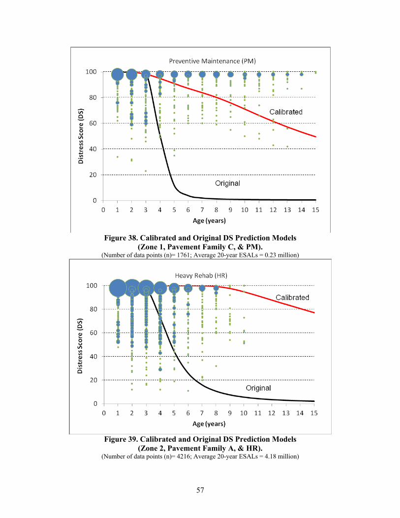
57


(Zone 1, Pavement Family C, & PM). (Number of data points (n)= 1761; Average 20-year ESALs = 0.23 million)



58





59





60





61

Figure 46. Calibrated and Original DS Prediction Models (Zone 2, Pavement Family B, & PM).

(Number of data points (n)= 735; Average 20-year ESALs = 2.77 million)



62



63


(Zone 2, Pavement Family C, & LR). (Number of data points (n)= 82; Average 20-year ESALs =1.94 million)

64

Figure 50. Calibrated and Original DS Prediction Models (Zone 2, Pavement Family C, & PM).

(Number of data points (n)= 310; Average 20-year ESALs = 1.36 million)



65





66





67





68





69





70





71




(Zone 4, Pavement Family A, & LR). (Number of data points (n)= 943; Average 20-year ESALs =5.73 million)

72





73





74





75



76





77

ASSESSMENT OF MODEL ERROR

Model error is measured as the difference between actual distress values and predicted distress values. This prediction error is defined as shown in Eq. 14.

(14)

where: e = the average prediction error. n = the total number of data points. Xi-predicted = the predicted value for ith section. Xi-actual = the actual value for ith section. In total, there are 914 distress prediction models (i.e., 914 sets of coefficients for various combinations of climate and subgrade zones, traffic level, treatment type, and pavement family). Considering all of these models, on average, the calibrated models have an error of ±8.3 percent (i.e., predicted distress is ±8.3 percent of actual distress). The original models have an average error of 19.9 percent (i.e., predicted distress is ±19.9 percent of actual distress). Figure 75 shows the frequency distributions of the model error for the original and calibrated models. It can be seen that the frequency distribution of the calibrated models error is significantly shifted to the left of the frequency distribution of the original models error. This signifies a major improvement to the in the models’ accuracy as a result of the calibration process.

Figure 75. Distribution of Standardized Model Error for Both Calibrated and Original Models.

78

SUMMARY AND CONCLUSIONS

TxDOT developed its existing pavement performance prediction models in the 1980s–1990s based on engineering judgment due to the lack of field performance data at that time. This report presents a process for calibrating these models using data extracted from PMIS and the results of applying this process to ACP in Texas. In this calibration process, a GA is used to determine the optimum model coefficients that minimize the model error (i.e., difference between actual and predicted performance). The GA was developed and coded in a software tool using the C# language. Because of the large number of model coefficients (more than 1000 coefficients are used for various combinations of distress types, pavement types, and M&R types) and the massive data that exists in PMIS, it was necessary to group the data into broader categories. These categories include climate, subgrade quality, pavement type, maintenance and rehabilitation type, traffic loading level, and distress type.

Based on the results of this study, the following conclusions can be made:

In all examined cases, the original models exhibited a pattern of predicting higher distress values (and consequently lower DS values) than the actual data (observed in the field).

The calibrated models predict less pavement deterioration compared to the original models (i.e., the calibrated models are not as severe as the original models).

The model’s standard error (i.e., difference between actual and predicted performance) was reduced significantly as a result of the calibration process. On average, the calibrated models have an error of ±8.3 percent (i.e., predicted distress is ±8.3 percent of actual distress); whereas the original models have an average error of 19.9 percent (i.e., predicted distress is ±19.9 percent of actual distress).

The original model coefficients do not ensure a logical performance pattern across treatment types: where heavy rehabilitation performs superior to medium rehabilitation, medium rehabilitation performs superior to light rehabilitation, and light rehabilitation performs superior to preventive maintenance. The calibrated models ensure that this logical performance pattern is maintained in all cases.

79

CHAPTER 5. CALIBRATION OF TXDOT’S CONTINUOUSLY REINFORCED CONCRETE PAVEMENT PERFORMANCE PREDICTION

MODELS

INTRODUCTION

This chapter documents the recalibration of continuously reinforced concrete pavement performance curves for PMIS. The purpose of the recalibration was to enhance current CRCP performance models to improve the reliability of pavement’s condition prediction. Performance curves were recalibrated for CRCP distress types and Ride Score using PMIS data from years 1993–2010. The recalibration process of the CRCP performance models was conducted using non-linear multi-regression for each of the 25 TxDOT Districts, 4 climate-subgrade zones, and statewide.

OVERVIEW OF PMIS CRCP PERFORMANCE CURVES

Performance curves are used to predict future pavement condition of Texas highways by projecting future distress ratings and Ride Scores. Through these predictions, pavement managers are able to plan future treatment and budget needs.

Performance curves relate pavement age to pavement distress through the following sigmoidal equation:

(15) where:

Li = level of distress in a pavement section or percent of ride quality lost for the distress and ride quality performance curves, respectively. alpha (α) = horizontal asymptote factor that represents the maximum range of distress growth. beta (β) = a slope factor that controls how steeply utility is lost in the middle of the curve. rho (ρ) = prolongation factor that controls the time it takes before significant increases in distress occur. chi (Χ ) = the traffic weighting factor that controls the effect of an 18-k ESAL on performance. epsilon (ϵ) = climate weighting factor that controls the effect of rainfall and freeze-thaw cycles on performance. (σ) = sub grade weighting support factor that controls the effect of sub grade strength on performance. Age = pavement age of section, in years.

The level of distress is obtained by “normalizing” the PMIS rating with the length of the pavement section (Eq. 16). Table 19 displays the criteria used for computing Li values for CRCP distress types.

80

Table 19. PMIS Rating for CRCP Distress Types.

(16)

Performance curves are used in PMIS to predict the amount of a given distress during the pavement’s life. The performance curve is described by a combination of coefficients for each particular distress. Table 20 displays the alpha, beta, and rho coefficients currently used statewide by PMIS for the CRCP performance curves for spalled cracks, punchouts, asphalt patches, and concrete patches. PMIS currently uses a value of 1 for the chi, epsilon, and sigma coefficients for all CRCP distresses.

Table 20. PMIS Performance Curve Coefficients for CRCP (Type 01). Distress Type Alpha Beta Rho Chi Sigma Rho

Spalled Cracks 1.690 22.090 10.270 1 1 1Punchouts 101.517 0.438 538.126 1 1 1Asphalt Patches 96.476 0.375 824.139 1 1 1Concrete Patches 146.000 1.234 40.320 1 1 1

The current CRCP PMIS performance curves for spalled cracks, punchouts, ACP patches, and Portland Cement Concrete (PCC) patches are shown in Figures 76–79, respectively.

81

Figure 76. PMIS Performance Curve for Spalled Cracks.

Figure 77. PMIS Performance Curve for Punchouts.

82

Figure 78. PMIS Performance Curve for ACP Patches.

Figure 79. PMIS Performance Curve for PCC Patches.

PROCEDURE TO CALIBRATE PAVEMENT DISTRESS PERFORMANCE MODELS

The steps to calibrate pavement performance models are outlined as follows:

1. Gather historical pavement distress information from PMIS records for a given District.

2. Perform a statistical analysis of the observed level of distress (Li) for each of the four CRCP distresses: spalled cracks, punchouts, ACP patches, and PCC patches. Mean, median, quartiles, maximum, minimum, and percentage of zeros were calculated in this analysis.

3. Review the results obtained from statistical analysis and receive feedback from experienced District personnel to identify critical age distress deterioration stages for setting a feasible range of performance curve coefficients to start the iterations for that District.

83

4. Determine the estimated age of the pavement sections. Since age is not included in the PMIS records and not all the Districts have this information available, then age is estimated with the following criteria:

a. If a pavement section initially demonstrates no distresses (Li = 0), then the fiscal year when the distress begins (Li>0) is given the age at which the distress deterioration starts.

b. Age increases according to the age increment between fiscal years. The age increment is initially set as one year. An age of zero is reset for a section when the Li decreases to zero.

5. Prepare Li and ΔLi data for regression analysis by filtering pavement distress data from outliers not representing the pavement distress evolution in the field.

6. Perform calibrations using non-linear multi-regression analysis. Two methods are used for this analysis: the Li Method and the ΔLi Method. The Li method consists of calibrating the estimated age directly with the observed Li values. The ΔLi method consists of calibrating the estimated age with the distress deterioration rate (ΔLi). ΔLi is calculated with Eq. 17.

(17) where:

= distress at the current year. = distress at the following year.

The ΔLi method consists was conceived as an alternative method in case non-linear multi-regression analysis for Li and Age directly did not show meaningful results.

PMIS DATA GATHERING AND DISTRESS STATISTICAL ANALYSIS

PMIS CRCP distress data were extracted for each of the 25 TxDOT Districts from FY1993 to FY 2010. There were 12,449 sections Statewide included in the distress statistical analysis. Histograms and box plots with quartiles were generated to study distress characteristics for spalled cracks, punchouts, ACP patches, and PCC patches.

Spalled Cracks

The Li spalled crack value has a large variation going from 0 to 1980 spalled cracks per mile. Seventy-one percent of the records report a Li value of 0. Figure 80 shows the histogram of the observed level of distress Li for spalled cracks. Figure 81 shows a relative frequency plot for this distress.

84

Figure 80. Histogram of Observed Li for Spalled Cracks.

Figure 81. Relative Frequency Plot of Observed Li for Spalled Cracks.

Seventy-five percent of the records reported two spalled cracks per mile or less. Table 21 shows a summary of the mean, standard deviation, minimum, maximum, median, first quartile, and third quartile of the Li for spalled cracks. Figure 82 shows the box plot of the Li values.

85

Table 21. Li Statistical Parameters for Spalled Cracks. Statistical Parameter Li

Mean 9.73Standard Deviation 45.73

Median 0Minimum 0Maximum 1980

1st Quartile 03rd Quartile 2

Frequency of Maximum 1

Figure 82. Box Plot of Observed Li for Spalled Cracks.

Punchouts

Eighty-nine percent of the PMIS records register zero punchouts. Figure 83 shows the histogram for Li for punchouts. Figure 84 shows a relative frequency plot for this distress.

86

Figure 83. Histogram of Li for Punchouts.

Figure 84. Frequency Plot of Li for Punchouts.

Table 22 displays the statistical parameters for the Li data of the punchout distress. Li ranges from 0 to 100 punchouts per mile with a mean of 0.54 and 2.57 as a standard deviation. Figure 85 shows the box plot for the punchouts data.

87

Table 22. Statistical Parameters for Li for Punchouts.

Statistical Parameter Li Mean 0.54

Standard Deviation 2.57Median 0

Minimum 0Maximum 100



Figure 85. Box Plot of Li for Punchouts.

ACP Patches

The number of records with ACP patches is minimal. Ninety-eight percent of records show a Li value of 0 for ACP patches. Figure 86 shows the histogram for the Li values for ACP patching. Figure 87 shows a relative frequency plot for this distress.

88

Figure 86. Histogram of Observed for ACP Patches.

Figure 87. Frequency Plot of Observed for ACP Patches.

Table 21 shows a summary of the statistical parameters for this distress. This distress does not show much variability. Figure 88 shows the box plot of Li for ACP patches.

89

Table 23. Li Statistical Parameters for ACP Patches.


Standard Deviation 2.08Median 0

Minimum 0Maximum 100



Figure 88. Box Plot of Observed Li for ACP Patches.

PCC Patches

Eighty-two percent of the PMIS records show no PCC patch. Figure 89 shows the histogram for the Li values for the PCC patches. Figure 90 shows a frequency plot for this distress.

90

Figure 89. Histogram of Li for PCC Patches.

Figure 90. Frequency Plot of Li for PCC Patches.

Table 24 presents the statistical parameters for the Li data of PCC Patches. There is a greater variability in the number of PCC patches per mile, which range from a minimum Li of 0 to a maximum of 205. Figure 91 shows the box plot for PCC patches.

91

Table 24. Li Statistical Parameters for PCC Patches. Statistical Parameter Li





Figure 91. Box Plot of Observed Li for PCC Patches.

Table 25 displays the number of sections for a District that demonstrate a Li greater than zero, the total number of sections in the District and the percentage of sections with an Li greater than zero. This is displayed for all the Districts fit for calibration. Districts displaying a hyphen are those Districts where no recalibrated performance curve was obtained due to the lack of data.

92

Tab

le 2

5. N

um

ber

of

Sect

ion

s w

ith

Lev

el o

f D

istr

ess

(Li)

Gre

ater

th

an Z

ero.

Dis

tric

ts

Sp

alle

d C

rack

s P

un

chou

ts

AC

P P

atch

es

PC

C P

atch

es

Li>

0 T

otal

P

erce

nta

ge

Li>

0 T

otal

P

erce

nta

ge

Li>

0 T

otal

P

erce

nta

ge

Li>

0 T

otal

P

erce

nta

ge

1 P

aris

51

16

0 32

%76

160

48%

- -

- 67

163

41%

2

For

t Wor

th

575

2165

27

%31

521

6315

%13

221

556%

576

2165

27%

3

Wic

hita

Fal

ls

245

484

51%

147

483

30%

- -

- 12

648

326

%

4 A

mar

illo

16

3 52

4 31

%48

515

9%-

- -

105

524

20%

5

Lub

bock

27

8 47

6 58

%84

476

18%

1646

93%

150

473

32%

6

Ode

ssa

1 10

10

%0

90%

- -

- -

- -

7 S

an A

ngel

o -

- -

- -

- -

- -

- -

- 8

Abi

lene

-

- -

- -

- -

- -

17

9

Wac

o 39

12

6 31

%-

- -

- -

- 31

110

28%

10

T

yler

27

86

31

%8

7311

%-

- -

1188

13%

11

L

ufki

n -

- -

- -

- -

- -

- -

- 12

H

oust

on

1305

37

37

35%

872

3737

23%

2337

291%

761

3737

20%

13

Y

oaku

m

54

163

33%

2315

615

%-

- -

2815

718

%

14

Aus

tin

9 28

7 3%

- -

- -

- -

- -

- 15

S

an A

nton

io

11

74

15%

- -

- -

- -

274

3%

16

Cor

pus

Chr

isti

-

- -

- -

- -

- -

- -

- 17

B

ryan

84

11

4 74

%32

105

30%

682

7%46

113

41%

18

D

alla

s 56

5 18

26

31%

- -

- -

- -

368

1824

20%

19

A

tlan

ta

34

84

40%

1084

12%

361

5%12

8514

%

20

Bea

umon

t 94

58

7 16

%11

258

519

%-

- -

103

587

18%

21

P

harr

3

6 50

%-

- -

- -

- -

- -

22

Lar

edo

1

23

4%-

- -

- -

- -

- -

23

Bro

wnw

ood

- -

- -

- -

- -

- -

- -

24

El P

aso

149

797

19%

101

795

13%

- -

- 12

279

715

%

25

Chi

ldre

ss

57

133

43%

3713

328

%-

- -

4413

433

%

Sta

tew

ide

3745

11

862

32%

1865

9474

20%

180

6496

3%25

5311

521

22%

93

From the statistical analysis performed in the Distress Score for Texas, it is observed that that CRCP sections are in good condition. Figures 92–94 show the histogram, relative frequency plots, and box plots. Seventy-eight percent of the Distress Score demonstrate to have a score of 100. The First Quartile of Distress Score started at 99 as shown in Table 26.

Figure 92. Histogram for CRCP Distress Scores, Statewide.

Figure 93. Relative Frequency Plot for CRCP Distress Score, Statewide.

94

Table 26. Statistical Parameters for CRCP Distress Score, Statewide.


Standard Deviation 20.07 Median 100

Minimum 1 Maximum 100

1st Quartile 99 3rd Quartile 100

Frequency of Maximum 83,936

Figure 94. Box Plot for CRCP Distress Scores, Statewide.

A statistical analysis was also performed for the Li of the Ride Score, statewide. Figures 95–97 show the histogram, relative frequency plot and box plot are used to summarize the data. The concentration of zeros is minimal when compared to the CRCP distresses. Only 0.2 percent of the data have a Li value of zero. Table 27 displays the statistical parameters.

95

Figure 95. Histogram of Li for CRCP Ride Scores.

Figure 96. Relative Frequency Plot of Li for CRCP Ride Scores.

Table 27. Li Statistical Parameters for CRCP Ride Scores. Statistical Parameter Li


Median 0.42Minimum 0 Maximum 1

1st Quartile 0.303rd Quartile 0.52


96

Figure 97. Box Plot of Li for CRCP Ride Score.

The Ride Score itself was also analyzed. Figures 98–100 show the histogram, relative frequency plot, and box plot. Most of the CRC pavement sections have a Ride Score between 3 and 4. Table 28 shows the statistical parameters.

Figure 98. Histogram for CRCP Ride Scores, Statewide.

97

Figure 99. Frequency Plot for CRCP Ride Scores, Statewide.

Table 28. Statistical Parameters for CRCP Ride Scores, Statewide. Statistical Parameter Li


Median 3.4Minimum 0.1Maximum 5

1st Quartile 33rd Quartile 3.8


Figure 100. Box Plot for CRCP Ride Scores, Statewide.

98

The Condition Score statewide was also analyzed. Figures 101–103 show the histogram, relative frequency plots, and box plots for the Condition Score. Fifty-one percent of the data have a Condition Score of 100. Table 29 presents the statistical parameters. It can be concluded from these results that most of the CRCP pavement sections in Texas are in a good condition.

Figure 101. Histogram for CRCP Condition Scores, Statewide.

Figure 102. Frequency Plot of CRCP Condition Scores, Statewide.

99

Table 29. Li Statistical Parameters for CRCP Condition Scores, Statewide. Statistical Parameter Li





Figure 103. Box Plot of Li for CRCP Condition Scores, Statewide.

Estimating Pavement Age

As the pavement age increases, the level of distress increases and the amount of utility decreases. The age at which distresses develop and the rate of distress increase vary according to the distress type. The distress starting age is a key factor in recalibrating the performance curve. According to the current PMIS performance curves, spalling develops around an age of nine years, punchouts at four years, asphalt patches at four years, and concrete patches at seven years. In order to determine this age, it is recommended to consult experienced District personnel and review historical records if available.

During the recalibration process, the theoretical age from the current PMIS performance curves was calculated for the Li data collected for each District. These data were plotted and used to determine an approximate distress starting age for each CRCP distress. From these analyses, the distress starting age was determined for each distress: at 9.5 years for spalled cracks and at 0 years for punchouts, ACP patches, and PCC patches. This information is used to start the iterations when conducting the non-linear multi-variable regression analysis.

100

The age associated to Li values was determined with the following criteria:

1. Age increases according to the age increment between fiscal years. For example, if data were collected for fiscal year 1995 and it is known that the pavement age is one year old, then the pavement age in 1996 is two years.

2. In a given section, an age of zero will be given to the year where the distresses decrease to an Li value of zero. For example, if a section had a distress of 14 spalled cracks per mile in 1997 and in 1998 the data showed no spalling, then it is assumed that the pavement has received major rehabilitation. As a result, the age of the pavement is restored back to 0 at the year at which the distress is no longer present. The age for the following years is then increased from that year (e.g., 0, 1, 2, 3…).

3. If a pavement section initially demonstrates no distresses (Li=0), then the year at which the distresses begin (Li>0) is given the age at which distress deterioration starts. This age is the distress starting age. The age for the previous and following fiscal years is then determined based on this distress starting age. If the distress starting age is zero, the first year at which distresses are recorded is set to zero.

Data Preparation

The next step in the calibration process is to prepare Li data for the non-linear multi regression analysis. Quartiles are used to filter outliers in the data sets. The Li data for a given distress type in the first and fourth quartile of each estimated age are removed. The data between the second and third quartiles of each estimated age is used in the recalibration process.

Due to the large concentration of records with Li = 0, the median of the observed Li values (for the Li Method) for each estimated age is calculated. The data set is reduced to a single representative Li values for each estimated age for the given distress type.

Non-Linear Multiple Regression Analysis

Non-linear multiple regression analysis is performed to recalibrate the PMIS CRCP distress performance curves. The method is applied using Li datasets filtered for first and fourth quartiles, and also for Li medians. Eq. 18 is used for the regression analysis of Li (Age):

(18) Table 30 shows a summary of the coefficients alpha (α), beta (β), and rho (ρ) obtained for the recalibrated CRC pavement distress performance models for spalled cracks, punchouts, PCC patches, and ACC patches in each of the 25 Districts and statewide. The R2–Median value presented in the table, measures how well the calibrated curve fits the Li Method data set for the Li medians. The R2–Quartile value shows how well the calibrated curve fits the Li Method data set for the Li data filtered for quartiles. The coefficients currently used by PMIS are also displayed

101

with the R2 measuring how well the PMIS curve fits the Li Method quartile data set. Districts displaying a hyphen are those Districts where a recalibration was not feasible due to limited distress data.

Table 30. Recalibration of CRCP Distress Performance Models.

Districts CRCP Distress Recalibrated Performance Curve Coefficients

α β ρ R²-Median R²-Quartile

01-Paris

Spalled Cracks 3.00 53.57 9.34 0.95 0.26Punchouts 8.00 123.44 12.87 0.95 0.51

ACP Patches - - - - -PCC Patches 2,643.55 0.95 73.09 0.94 0.81

02-Fort Worth


ACP Patches 11,694.17 1.41 72.57 0.66 0.45PCC Patches 4.46 32.95 15.89 1.00 0.43

03-Wichita Falls


ACP Patches - - - - -PCC Patches 4.09 24.07 12.61 0.99 0.40

04-Amarillo



05-Lubbock


ACP Patches 15,045,539 0.17 247,096,415.20 0.35 0.14PCC Patches 396.00 0.65 151.19 0.80 0.46

06-Odessa

Spalled Cracks 4.04 43.75 9.42 1.00 0.09Punchouts - - - - -

ACP Patches - - - - -PCC Patches - - - - -

07-San Angelo

Spalled Cracks - - - - -Punchouts - - - - -


08-Abilene



102

Table 30. Recalibration of CRCP Distress Performance Models (Continued).



09-Waco



10-Tyler



11-Lufkin



12-Houston


ACP Patches 71.58 19.82 17.93 1.00 1.00PCC Patches 4,918.58 0.99 112.06 0.96 0.51

13-Yoakum

Spalled Cracks 2,538.82 0.49 389.27 0.75 0.62Punchouts 59.72 14.79 16.29 1.00 0.42

ACP Patches - - - - -PCC Patches 171,632.50 0.25 220,138.48 0.31 0.03

14-Austin



15-San Antonio



16-Corpus Christi

Spalled Cracks

District 16 does not have CRC pavement. Punchouts

ACP Patches PCC Patches

17-Bryan


ACP Patches 2.00 124.04 13.24 1.00 1.00PCC Patches 17.50 159.26 11.02 0.55 0.58

103

Table 30. Recalibration of CRCP Distress Performance Models (Continued).



18-Dallas



19-Atlanta



20-Beaumont


ACP Patches - - - - -PCC Patches 95,923.650 0.323 9766.617 0.640 0.430

21-Pharr



22-Laredo



23-Brownwood

Spalled Cracks



24-El Paso

Spalled Cracks 2.20 79.28 9.22 0.96 0.27Punchouts 34,239.33 0.26 147,796.12 0.40 0.14


25-Childress



Statewide



Current PMIS

Spalled Cracks 1.69 22.09 10.27 - 0.552Punchouts 101.517 0.438 538.126 - 0.344

ACP Patches 96.476 0.375 824.139 - -PCC Patches 146.000 1.234 40.320 - 0.452

Figures 104–107 show the best fit recalibrated distress statewide performance curves for spalled cracks, punchouts, PCC patches, and ACP patches, respectively.

104

Figure 104. Recalibrated CRCP Spalled Cracks Performance Curve,

Statewide, Median Method (Unconstrained).

Figure 105. Recalibrated CRCP Punchouts Performance Curve,


105

Figure 106. Recalibrated CRCP ACP Patches Performance Curve,


Figure 107. Recalibrated CRCP PCC Patches Performance Curve,


In a second analysis, we limited the maximum range of distress growth by constraining the value of alpha. Alpha values were constrained within a 90 percent confidence interval. Eq. 19 was used to calculate the maximum limit for the alpha value.

(19)

Table 31 shows a summary of the recalibrated coefficients for CRCP distress performance curves obtained for each of the 25 Districts and statewide. The R² values for the Li Method data set for the median method and quartile method are presented. Districts displaying a hyphen are those Districts where a calibration was not feasible due to limited distress data.

106

Table 31. Recalibration of CRCP Distress Performance Models with Constrained Parameters.



01-Paris



02-Fort Worth



03-Wichita

Falls



04-Amarillo



05-Lubbock



06-Odessa



07-San Angelo



08-Abilene



107

Table 31. Recalibration of CRCP Distress Performance Models with Constrained Parameters (Continued).



09-Waco



10-Tyler



11-Lufkin



12-Houston



13-Yoakum



14-Austin



15-San Antonio



16-Corpus Christi

Spalled Cracks



17-Bryan



108

Table 31. Recalibration of CRCP Distress Performance Models with Constrained Parameters (Continued).



18-Dallas



19-Atlanta



20-Beaumont



21-Pharr



22-Laredo



23-Brownwood

Spalled Cracks



24-El Paso



25-Childress



Statewide



Figures 108–111 show the best fit recalibrated statewide distress performance curves for the constrained method for spalled cracks, punchouts, PCC patches, and ACC patches, respectively.

109

Figure 108. Recalibrated CRCP Spalled Cracks Performance Curve,

Median Method, (Constrained).

Figure 109. Recalibrated CRCP Punchouts Performance Curve,


110

Figure 110. Recalibrated CRCP ACP Patches Performance Curve,


Figure 111. Recalibrated CRCP PCC Patches Performance Curve,


The performance curves were revised and recalibrated based on feedback from TxDOT personnel and statistical analysis of PMIS data. In the recalibration, the beta (β) parameter was constrained to 50.

The recalibrated CRCP distress performance curves are based on the following reasoning:

1. For the spalled cracks performance curve, it was concluded that the most representative distress model is the unconstrained curve. According to feedback from TxDOT pavement experts, this curve represents the slow appearance of this distress.

111

2. The alpha (α) of the punchouts performance curve was constrained to 2. Given that punchouts are a serious structural distress and that they need to be addressed quickly, the performance curve limit the maximum number of acceptable punchouts to 2.

3. The alpha (α) of the ACP patches performance curve was constrained to 1 since according to the statistical analysis performed this distress is not very common in CRC pavements. Ninety-eight percent of the data analyzed showed no ACP patching distress (ACP patch Li was equal to zero). This constraint was also found reasonable according to feedback from TxDOT pavement experts. The rho (ρ) parameter was also constrained to less than 15 to control the age at which ACP patches start to occur (distress starting age). Given that patches are used to address punchout problems, it is reasonable for punchouts to start earlier than ACP patches.

4. According to feedback from TxDOT pavement experts, the alpha (α) of the PCC patches performance curve was suggested to be constrained at 4.

Figures 112–115 shows the final recalibrated CRCP distress performance curves recommended statewide.

Figure 112. Recommended Statewide CRCP Spalled Cracks Performance Curve, Median Method.

112

Figure 113. Recommended Statewide CRCP Punchouts Performance

Curve, Median Method.

Figure 114. Recommended Statewide CRCP ACP Patches Performance


113

Figure 115. Recommended Statewide CRCP PCC Patches Performance


Table 32 shows the coefficients for the final recalibrated statewide CRCP distress performance curves.

Table 32. Recommended Statewide CRCP Performance Curve Coefficients.

CRCP Distress Recalibrated Statewide Performance Curve Coefficients α β ρ R²-Median R²-Quartile



Distress Score, Ride Score, and Condition Score

Once the distress performance curves are recalibrated, the performance models can be used to estimate future needs for pavement sections. The performance curves are used to determine the following: (a) the current age of the pavement for each distress type, (b) the level of distress (Li) for the predicted needs estimate age (predicted age=current age + additional number of years to the year where the needs estimate is to be predicted), and (c) future utility value for the needs estimate.

Once the utility value is obtained for each distress type, the Distress Score for the pavement section can be predicted. The Distress Score is calculated using Eq. 20.

(20)

where U is the utility of the given distress type obtained with Eq. 21.

114

(21)

The coefficients in Eq. 21 retain the same meaning as those described in Eq. 16 while Li is the level of distress for the given distress type.

Using the Ride Score utility value and the Distress Score, the Condition Score of the pavement section is calculated with Eq. 22.

(22)

Before determining the Condition Score, the Ride Score performance curves need to be calibrated. As a result, calibration of the Ride Score performance curves was also performed. The following steps outline the process followed to recalibrate the Ride Score curves:

1. The traffic level for each pavement section was classified into “Low” (ADT × Speed Limit≤27,500), “Medium” (27,501<ADT × Speed Limit≤165,000), and “High” (ADT × Speed Limit>165,000).

2. According to the traffic level classification, the percent of ride quality lost (Li) for the Ride Score (RS) was obtained using Eq. 23 and Table 33. Table 33 displays the minimum Ride Score (RSmin) for each of the traffic levels. There are two existing special cases of the Li calculation that need to be addressed differently. First, if the calculated Li is greater than or equal to one (or in other words, Ride Score is less than or equal to RSmin), then Li is set equal to one. Second, if the calculated Li is less than or equal to zero (or in other words, the Ride Score is greater than or equal to 4.8), then Li is set equal to zero.

(23)

Table 33. RSmin Value for Calculating Level of Distress (Li) according to Traffic Category.

PMIS Traffic Class RSmin Value Low 0.5

Medium 1.0High 1.5

3. The same data filter process applied to Li for CRCP distresses was applied to the ride Li. The same age assumptions were also used to determine the pavement age. A distress starting age of zero was used in these assumptions.

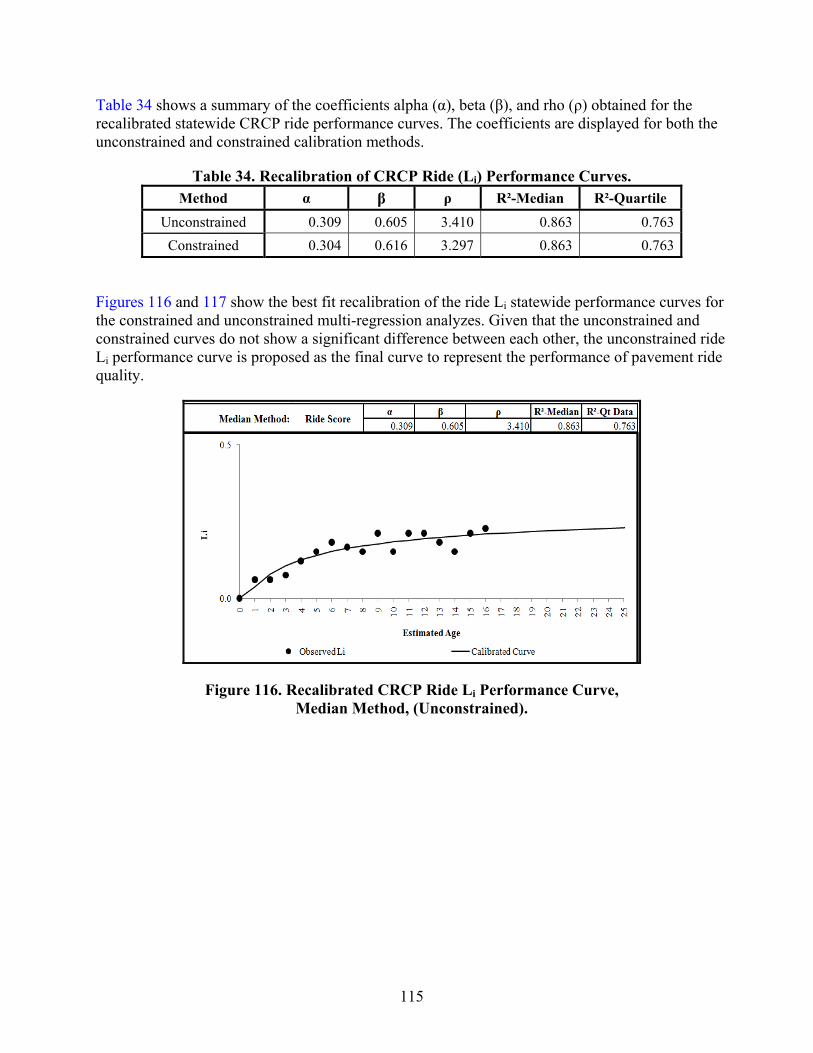
115

Table 34 shows a summary of the coefficients alpha (α), beta (β), and rho (ρ) obtained for the recalibrated statewide CRCP ride performance curves. The coefficients are displayed for both the unconstrained and constrained calibration methods.

Table 34. Recalibration of CRCP Ride (Li) Performance Curves. Method α β ρ R²-Median R²-Quartile

Unconstrained 0.309 0.605 3.410 0.863 0.763

Constrained 0.304 0.616 3.297 0.863 0.763

Figures 116 and 117 show the best fit recalibration of the ride Li statewide performance curves for the constrained and unconstrained multi-regression analyzes. Given that the unconstrained and constrained curves do not show a significant difference between each other, the unconstrained ride Li performance curve is proposed as the final curve to represent the performance of pavement ride quality.

Figure 116. Recalibrated CRCP Ride Li Performance Curve, Median Method, (Unconstrained).

116

Figure 117. Recalibrated CRCP Ride Li Performance Curve, Median Method, (Constrained).

Climate and Subgrade Zones

Recalibration was also performed based on climate and subgrade zones to obtain curves that are representative of the effects of temperature, moisture, and subgrade quality on CRCP. Counties in Texas were divided into the zones according to similar climate and subgrade characteristics. Table 35 describes the characteristics for each zone. Table 36 presents the 254 counties grouped in each of the four zones. Figure 118 presents the areas of the zones.

Table 35. Climate and Subgrade Characteristics for Zones. Zone Climate and Subgrade Characteristics

Zone 1 Wet-cold climate and poor, very poor, or mixed subgrade Zone 2 Wet-warm climate and poor, very poor, or mixed subgrade Zone 3 Dry-cold climate and good, very good, or mixed subgrade Zone 4 Dry-warm climate and good, very good, or mixed subgrade

117

Table 36. Counties in Climate and Subgrade Zones. Zone Counties

Zone 1 1, 19, 32, 34, 37, 43, 57, 60, 61, 71, 73, 75, 81, 92, 93, 103, 108, 112, 113, 117, 120, 127, 130, 139, 155, 172, 175, 182, 183, 184, 190, 194, 199, 201, 212, 213, 220, 225, 230, 234, 249, 250

Zone 2 3, 4, 8, 11, 13, 20, 21, 26, 28, 29, 36, 45, 62, 74, 76, 80, 82, 85, 87, 89, 90, 94, 98, 101, 102, 106, 110, 114, 121, 122, 124, 126, 129, 137, 143, 144, 145, 146, 147, 149, 154, 158, 166, 170, 174, 176, 178, 181, 187, 196, 198, 202, 203, 204, 205, 210, 228, 229, 235, 236, 237, 239, 241

Zone 3 5 , 6, 9, 12, 14, 16, 17, 18, 23, 25, 27, 30, 33, 35, 38, 39, 40, 42, 44, 47, 49, 50, 51, 54, 56, 58, 59, 63, 65, 68, 77, 78, 79, 84, 86, 91, 96, 97, 99, 100, 104, 105, 107, 111, 115, 118, 128, 132, 135, 138, 140, 141, 148, 150, 152, 153, 157, 160, 161, 167, 168, 169, 171, 173, 177, 179, 180, 185, 188, 191, 197, 206, 208, 209, 211, 215, 217, 219, 221, 223, 224, 227, 242, 243, 244, 246, 251, 252

Zone 4 2, 7, 10, 15, 22, 24, 31, 41, 46, 48, 52, 53, 55, 64, 66, 67, 69, 70, 72, 83, 88, 95, 109, 116, 119, 123, 125, 131, 133, 134, 136, 142, 151, 156, 159, 162, 163, 164, 165, 186, 189, 192, 193, 195, 200, 207, 214, 216, 218, 222, 226, 231, 232, 233, 238, 240, 245, 247, 248, 253, 254

Figure 118. Climate and Subgrade Zones Utilized for Recalibration of CRCP Performance Curves.

118

After grouping the distress data according to zones, the CRCP distresses were calibrated using the methods previously presented. The same age assumptions were also used to determine the pavement age and a distress starting age of zero was used for these assumptions. The calibrated curves were determined for both the constrained and unconstrained alpha parameter. Tables 37 and 38 present the results obtained from the calibration for both approaches, respectively.

Table 37. Recalibration of CRCP Performance Curves for Zones.

Zone CRCP Distress Recalibrated Performance Curve Coefficients


Zone 1



Zone 2


ACP Patches 71.58 19.818 17.93 1 1PCC Patches 585.746 1.207 58.058 0.943 0.468

Zone 3

Spalled Cracks 4.166 94.121 9.182 0.860 0.597Punchouts 7.436 30.341 17.15 1 0.992

ACP Patches 1.8E-13 0.65692 1.21 - 0.0011PCC Patches 7.338 4.957 13.884 0.870 0.567

Zone 4

Spalled Cracks 2.200 79.276 9.223 0.964 0.275Punchouts 393333 0.224 1696612 0.406 0.142


Table 38. Recalibration of CRCP Performance Curves for Zones with Constrained Parameters.

Zone CRCP Distress Recalibrated Performance Curve Coefficients


Zone 1



Zone 2



Zone 3



Zone 4



119

CONCLUSIONS

1. PMIS raw data from 1993–2010 show a large amount of records with no distresses (71 percent for spalled cracks, 89 percent for punchouts, 98 percent for ACP patches, and 83 percent for PCC patches). This situation reflects the importance of the pavement sections where CRP pavements are located (interstates, state highways), which demand immediate repair from TxDOT (especially punchouts). The lack of data at a later deterioration stage makes it challenging to develop performance curves to forecast future distresses. In reality, CRCP pavements are not allowed to deteriorate without being repaired by TxDOT in the short term. These observations will be used in Phase III of the project where decision trees will be improved. The trigger values used in the Needs Estimate decision trees will be modified according to these conclusions.

2. The recalibrated CRCP distress performance curves presented here represent an improvement when compared to the current distress performance curves since the analysis was conducted with a larger dataset. Further refinement of the CRCP performance curves will require additional feedback from TxDOT Districts and external CRCP experts. In the current analysis, alpha values were constrained, but they could be further adjusted based on local experience at each District. Rho, which is the prolongation factor that controls the time the pavement takes before significant increases in distress occur, could also be further adjusted based on additional local information from each District.

3. The initial Ride Score for a CRCP is mainly affected by factors acting during construction, and then its decline in ride quality is influenced by the quality of patches and the presence of distresses (spalling and punchouts) as well as the effect of expansive soils if such soils were not properly stabilized. Since there are not many distresses manifested for CRCP according to the PMIS records (75 percent of the data have a Distress Score of 100) due to TxDOT maintenance policies, the Condition Scores observed in the database for CRCP were more sensitive to changes in the Ride Score. For CRCP only 0.2 percent of the ride Li have a value of zero, and 51 percent of the data have a Condition Score of 100.

4. The methodology followed for the recalibration of CRCP performance curves could also be applied to other pavement types.

5. TxDOT personnel indicated that the coefficients in Table 37 and Table 38 will be considered for use for PMIS. These tables are also included in Appendix J. As indicated in conclusion 2, additional feedback from TxDOT Districts and external CRCP experts is needed to determine if further refinement is needed for these coefficients.

121

CHAPTER 6. CALIBRATION OF TXDOT’S JOINTED CONCRETE PAVEMENT PERFORMANCE PREDICTION MODELS

INTRODUCTION

TxDOT routinely collects distress data during annual field surveys statewide, storing them in TxDOT’s PMIS database. PMIS has five distress prediction models and one Ride Score loss model for JCP. PMIS models, developed in the 1990s, are still in use for both JCP types and all traffic levels, maintenance strategies, and climatic zones (Stampley et al. 1995).

However, since the time these performance prediction models were developed, TxDOT has accumulated a wealth of additional pavement performance data from their annual field surveys. The broad objective of this project was to calibrate the existing models for all pavement types, using historical PMIS distress data.

For JCP, the goal was more than recalibration; it also included disaggregating the data into modeling groups consisting of all combinations of traffic levels, maintenance strategies, JCP types, and climatic zones. Figure 119 illustrates the 72 possible combinations, which would result in a total of 1296 recalibrated coefficients for 432 JCP models. Please note that there were no JCP sections present in Zone 4 at the time of this analysis. If such pavements are constructed in Zone 4 in the future, the researchers recommend using Zone 3 coefficients. The performance prediction coefficients are in Appendix K.

2

1

Low Medium

PM

LR

HR

HR

3

32

2JCPtypes

3zones

3trafficlevelsHeavy

4treatments:PM=preventivemaintenanceLR=lightrehabilitationMR=mediumrehabilitationHR=heavyrehabilitation

Foreachdistress,model:

Figure 119. Modeling Groups and Grouping Factors.

122

JCP DISTRESS TYPES AND EVALUATION IN PMIS

Table 39 summarizes the JCP distress manifestations defined and recorded in PMIS, with their most commonly used abbreviations and units of measurement. It also shows how they transition into other categories as the pavement gets worse (e.g., failed joints and cracks becoming failures) or the pavement is treated (e.g., failures becoming patches).

PMIS performance evaluation is based on two indices, the Distress Score and the Condition Score, respectively, calculated according to Eqs. 24 and 25. Both indices rate the pavements from 0 to 100 and are interpreted as depicted in Table 40.

5

1iiUDS

(24) where:

Subscript “i” refers to the JCP distress manifestations listed in Table 39.

Ui are utility values between 0 and 1, calculated for the observed level of each distress “i” using utility functions that were also updated in this project.

The CS is the product of DS and the Ride Score utility RSu:

CS=DS*RSu (25)

Utility functions were also updated in this project based on results of a utility questionnaire and of project-specific field surveys by TxDOT’s experts.

DISTRESS PREDICTIONS IN PMIS

PMIS currently has one JCP model for each distress manifestation, in use for all traffic levels and maintenance strategies. All models follow Eq. 26. One of this project’s objectives was to recalibrate Eq. 26 using a 17-year historical database, defining models for each combination of traffic level, climatic zone, and maintenance strategy. The original models are discussed in conjunction with the recalibrated models.

age

iL e (26)

where:

Li = the level (L) of each JCP distress manifestation “i.”

age = pavement age.

e = 2.7182818…

α, σ, and β = model coefficients recalibrated in this project.

123

Table 39. JCP Distress Manifestations in PMIS.

JCP distress Brief description May progress into

Failed Joints & Cracks (FJC) % failed

Spalled and/or unsealed joints and transverse cracks that still transfer load

Failure

Failures (F, FL) number / mile

Distresses resulting in load transfer loss: punchouts, asphalt patches in any condition, faulted joints or cracks, failed concrete patches, D-cracking, wide or large spalls, etc.

Patch Shattered slab

Shattered slabs (S, SS) % slabs

Any slab with five or more failures or with failures covering half or more of the slab.

Concrete Patches (P, CP, PAT, CPAT) Number / mile

Any concrete patch longer than 10 in., rated as one patch for every 10 ft in length. Patch width is not considered.

Failure Shattered slab

Longitudinal Cracks % slabs with LC

Cracks parallel to the highway centerline. Failure Patch

Source: TxDOT PMIS Rater’s Manual 2010 (summary of contents) Note: Ride Score is also measured (0 to 5)

Table 40. PMIS Scores Interpretation. Class Description Distress Score Condition Score

A Very Good 90–100 90–100 B Good 80–89 70–89 C Fair 70–79 50–69 D Poor 60–69 35–49 F Very Poor ≤59 1–34

Source: TxDOT PMIS Manua1 1997, page 2-13,

MAINTENANCE AND REHABILITATION TREATMENTS IN PMIS

PMIS uses the five treatment categories listed below for all pavement types. Table 41 lists the various JCP treatments and their corresponding PMIS treatment codes. Applied treatments are not recorded in PMIS.

124

Table 41. JCP Treatments and Corresponding PMIS Intervention Levels. JCP TREATMENT PMIS Code

None NN

Grooving and Grinding PM

Joint Sealing PM

Repair of Spalled Cracks or Joints PM

Full Depth Repair of Concrete Pavement (FDRCP) LR

Partial depth patch LR or PM

ACP Overlay LR

FDRCP and ACP Overlay MR

Mill and ACP Overlay MR

Unbonded Concrete Overlay HR

Bonded Concrete Overlay HR

Reconstruction HR Needs nothing (NN); Preventive Maintenance (PM); Light Rehabilitation (LR); Medium Rehabilitation (MR); Heavy Rehabilitation (HR).

Source: various TxDOT District personnel (this project’s interviews and surveys).

METHODOLOGY

The methodology used for data treatment and subsequent modeling consisted of the following steps:

1. Estimate JCP age (not available in PMIS) based on 580 JCP sections with construction dates (see Data Treatment).

2. Treat the distress data to minimize the influence of maintenance policies as well as of one distress type evolving into another (see Table 39).

3. Estimate JCP treatments (not available in PMIS) based on Distress Scores and distress evolution (see Data Treatment).

4. Test the significance of modeling factors (JCP types, climatic zones, traffic levels, and maintenance) in overall JCP performance, grouping factors where applicable (see Modeling Groups).

5. For each distress and modeling group:

a. Examine the data for adherence to the expected order of performance, from best to worst: HR > MR > LR > PM Low traffic > medium traffic > heavy traffic.

b. Check for statistical significance of modeling factors (zone, traffic, etc.) in each distress manifestation, grouping them for that particular distress manifestation when applicable.

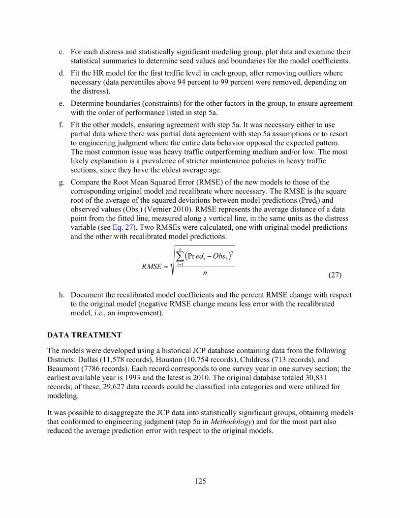
125

c. For each distress and statistically significant modeling group, plot data and examine their statistical summaries to determine seed values and boundaries for the model coefficients.

d. Fit the HR model for the first traffic level in each group, after removing outliers where necessary (data percentiles above 94 percent to 99 percent were removed, depending on the distress).

e. Determine boundaries (constraints) for the other factors in the group, to ensure agreement with the order of performance listed in step 5a.

f. Fit the other models, ensuring agreement with step 5a. It was necessary either to use partial data where there was partial data agreement with step 5a assumptions or to resort to engineering judgment where the entire data behavior opposed the expected pattern. The most common issue was heavy traffic outperforming medium and/or low. The most likely explanation is a prevalence of stricter maintenance policies in heavy traffic sections, since they have the oldest average age.

g. Compare the Root Mean Squared Error (RMSE) of the new models to those of the corresponding original model and recalibrate where necessary. The RMSE is the square root of the average of the squared deviations between model predictions (Predi) and observed values (Obsi) (Vernier 2010). RMSE represents the average distance of a data point from the fitted line, measured along a vertical line, in the same units as the distress variable (see Eq. 27). Two RMSEs were calculated, one with original model predictions and the other with recalibrated model predictions.

n

ObsedRMSE

n

iii

1

2Pr

(27)

h. Document the recalibrated model coefficients and the percent RMSE change with respect

to the original model (negative RMSE change means less error with the recalibrated model, i.e., an improvement).

DATA TREATMENT

The models were developed using a historical JCP database containing data from the following Districts: Dallas (11,578 records), Houston (10,754 records), Childress (713 records), and Beaumont (7786 records). Each record corresponds to one survey year in one survey section; the earliest available year is 1993 and the latest is 2010. The original database totaled 30,831 records; of these, 29,627 data records could be classified into categories and were utilized for modeling.

It was possible to disaggregate the JCP data into statistically significant groups, obtaining models that conformed to engineering judgment (step 5a in Methodology) and for the most part also reduced the average prediction error with respect to the original models.

126

Modeling Groups

The two JCP types were grouped to ensure sufficient data to model by zone, as well as consistency across zones, based on the following facts:

About 85 percent of the available data are JCP type 2. There are no JCP type 3 data for Zone 3. Less than 7 percent of the JCP data in Zone 2 are type 3. Statistical tests of Distress Score differences by JCP type were not significant for PM or

HR in Zone 1.

Class variable zone was not significant for Distress Score in the HR dataset (P-value=0.4136, Kruskal-Wallis test; statistical significance starts at P-value≤0.05). This agrees with the expectation that new and/or reconstructed JCP should perform well regardless of zone.

The other combinations of zones and traffic levels were significant for overall performance (Distress Score) and were retested on a distress-by-distress basis. In some cases, two or more zones and/or traffic levels could be grouped, as discussed later under “Updated Models.” Table 42 summarizes the modeling groups and the number of data points available.

Table 42. Summary of Modeling Groups.

Heavy Traffic

Medium Traffic

Low Traffic

Total by Treatment

Zone 1 364 2,102 1,735

PM Zone 2 1,566 2,633 2,818 11,787

Zone 3 40 25 504

Zone 1 731 1,079 1,249

LR Zone 2 2,214 2,127 2,513 10,020

Zone 3 81 0 26

HR All 3,269 2,316 2,235 7,820

Total by Traffic Level 8,265 10,282 11,080 29,627

Traffic Level

Cumulative ESALs are recorded in PMIS, and traffic levels are defined as follows:

Low Traffic: less than 1.0 million ESALs (11,080 records). Medium Traffic: greater than or equal to 1.0 million and less than 10 million ESALs

(10,282). Heavy Traffic: greater than or equal to 10 million ESALs (8265).

127

Pavement Age

Since pavement age is not available in PMIS, the researchers procured a dataset containing construction dates of 580 JCP sections. Pavement age is fiscal year (of the survey) minus year built. After merging with the historical data base and eliminating inconsistent data (such as negative ages), 2,750 ages of 558 sections could be used to estimate JCP age. These data were used as a basis to estimate the age of the remaining records. Eq. 28 depicts the best regression model for JCP age (R2=56 percent, all coefficients’ P-values less than 0.0001).

(28) where: FJCadj = failed joints and cracks (adjusted and no outliers). Padj = patches (adjusted and no outliers). FLadj = failures (adjusted and no outliers). Shattered slabs (SS) and longitudinal cracks (LC) are both zero for over 90 percent of the data records and as a result were not significant in fitting the age model. For example, the P-value for the LC coefficient in the first modeling attempt using all distresses was 0.5730 (statistical significance requires a P-value of 0.05 or less). JCP Ride Scores tend to remain constant with time; adding Ride Score loss to the model resulted in inconsistent age estimates.

Figure 120 shows the plot of predicted versus observed values and the line of equality (in blue). There is significant data scatter; not surprisingly, the average prediction error is 5 years (calculated according to Eq. 27). Nevertheless, using these age estimates instead of elapsed times between surveys made JCP distress modeling feasible.

Age=0 was not assigned using Eq. 28; rather, age=0 was assigned using the criteria for heavy rehabilitation (HR) detailed in Table 43 under JCP Treatment Estimates.

Eq. 28 should not be used directly with distress data from PMIS; it was developed using distress values adjusted to minimize impacts of maintenance measures on distress evolution, as well distress category changes, as discussed under Adjusted Distress Data.

Eq. 28 works best within the following ranges: pavements 12-years old or younger (nearly 85 percent of the data was in that age range) and distress levels below their 95 percent percentile. It is not valid to estimate age=0.

128

‐5

0

5

10

15

20

25

‐5 0 5 10 15 20 25

Estimated Age

(years)

Observed Age (years)

Figure 120. Observed versus Estimated JCP Ages.

Adjusted Distress Data

The JCP models intend to capture distress progression as the pavement ages, but careful examination of the distress data indicated that distress levels often change due to:

TxDOT’s good maintenance practices. The definition of JCP distresses in PMIS.

JCP distresses progress as charted in Figure 121. For example, “failed joints and cracks” may progress into failures, then into patches, which may revert to failures and then be patched again (TxDOT 2010).

FailedJointsandCracks

Failures

LongitudinalCracks

ConcretePatches

ShatteredSlabsApparentJointSpacing

Figure 121. JCP Distress Progression.

Moreover, distress quantities measured per slab are calculated as a function of the apparent joint spacing (AJS), which is the distance between transverse cracks wide enough to prevent load transfer (see Eq. 29). If AJS increases, the amount of distress per “apparent” slab also increases.

129

Theoretically, this could not happen, but crack width varies with the slab temperature so the AJS increases observed in PMIS are possible due to temperature differentials among different survey days. In addition, cracks can be sealed, cross-stitched, etc., so AJS can revert to the original distance between joints.

(29) where:

L = distress quantity in PMIS. Rat = survey rating. Len = section length in miles. AJS = apparent joint spacing. Clearly, it was necessary to adjust the distress histories to minimize the influence of maintenance practices and distress type changes, thus ensuring that the models would accurately reflect distress progression with time rather than maintenance practices, distress type change, and/or environmental differences in crack widths defining the AJS.

Distress data treatment consisted of two steps:

1. Ensure consistency in AJS history, recalculating the distress quantities where needed.

2. More importantly, minimize the influence of maintenance and of distress evolution into another type by maintaining the previous distress observation every time a distress decreased. Using failed joints and cracks as an example, FJCi≥FJCi-1 for every survey year.

Using data where some observations are equal to or greater than their value in the database and others are equal to that value is a statistical technique called “censoring.” It is commonly used for modeling life-span and reliability, where experiments usually end before all subjects “fail” or “die.” Censoring extracts every bit of information provided by the data and is especially useful when it is necessary to extrapolate beyond the existing data range (Kalbfleisch et al. 1980; Klein et al. 1997).

JCP Treatment Estimates

Unlike pavement age, there are no M&R treatment data for any subset of the historical JCP database. Therefore, it was necessary to assign treatments based on logical deductions from Distress Scores and distress manifestation histories. Table 43 show the criteria used to assign treatments and the number of records obtained for each treatment.

130

Table 43. M&R Treatment Criteria.

M&R Category

Criteria and Assumptions Historical

Data Records

HR

New pavements (ages known, see Pavement Age section) HR treatment year and age=0 assigned based on the following criteria:

No distresses. Condition score (CS)=100. Distresses more serious than FJC and LC in the year preceding

treatment.

2,750 5,070

MR MR for JCP consists of flexible overlays, so data is no longer stored as JCP.

None

LR Section’s average Distress Score above the lower quartile and not meeting any HR assumptions.

10,020

PM Section’s average Distress Score below the lower quartile. 11,787 TOTAL 29,627

UPDATED MODELS

Distress Manifestations

Appendix K contains a table (formatted in 8.5 in. by 14 in.) depicting the updated and original model coefficients for each statistically significant model group (see Eq. 26). It also documents the number of data records used in the recalibration, and the percent change in RMS error with respect to the original model (see Eq. 27).

The analysis generated 66 new distress models, with a total average improvement in RMSE of 27.72 percent when compared to the original models. Appendix L presents plots comparing the distress data, the fitted model and the original model, as well as plots comparing updated and original models in each treatment group.

Eighty-nine percent of the 66 updated models (59 models) showed an improvement in the RMSE when compared with the original models (percent RMSE change depicted in Appendix K is negative). In one case, the original model was recommended. The remaining six models increased the RMSE when compared to the original models. Error increases occurred where it was impossible to simultaneously achieve error reduction and compatibility with the logical performance order by traffic level and by M&R treatment (see step 5 in Methodology).

Figure 122 illustrates this issue. It depicts all data points available for Zone 3, light rehabilitation (there is no medium traffic in this group). This group was selected as an example because the fact that heavy traffic outperformed low traffic for all ages is easily visible. In order to reduce the error, it would be necessary to improve model agreement with the data. However, the updated models must meet the reverse underlying assumption (heavy traffic causes more failures). Considering that the average age of the heavy traffic sections is the highest, the only logical explanation for this behavior would be stricter maintenance policies in heavy traffic areas.

131

‐4

‐2

0

2

4

6

8

10

12

14

16

‐3 ‐2 ‐1 0 1 2 3 4 5 6 7 8 9 10 11 12 13 14 15 16 17 18 19

Failures / mile

Age

Heavy Traffic Data, 81 observations

Low Traffic Data, 26 observations

Original Model

Figure 122. Failures in Zone 3, Light Rehabilitation.

Figure 123 compares a bubble plot of the data scatter, the updated and the original model, for failed joints and cracks. In this example, the updated model predicted more FJC at early ages and less at later ages, achieving a 36.4 percent improvement in prediction error. Clearly, there is considerable data scatter around all improved models (see Appendix L), which was unavoidable, given the nature of the distress data and the fact that hard data on pavement age as well as on M&R treatment are not available in PMIS.

Figures 124–135 in the next sections present the updated models for each distress manifestation in more detail, discussing their principal characteristics as compared to the original models. Please note that these figures’ legends use the abbreviations and color coding listed below.

Original models are thin black lines. M&R treatments: PM models are thick solid lines, LR models are thin solid lines, and

HR models are dotted lines. Traffic levels: L, M, and H, respectively, in green, orange, and red. Grouped traffic levels are color-coded in blue for L&M and in brown for M&H. Other groupings are color-coded in shades of purple and pink.

132

‐20

‐10

0

10

20

30

40

50

60

70

80

90

100

‐2 0 2 4 6 8 10 12 14 16 18 20 22

Failed Joints and Cracks (%

)

Age

Low Traffic Data

Original Model

Low Traffic Model

Figure 123. FJC Model for Zones 2 and 3, Light Rehabilitation, Low Traffic.

Failed Joints and Cracks

Fifteen new models were developed for this distress manifestation, with an average RMSE improvement of 17.65 percent over all models. They are depicted in Figure 124 (Zone 1) and Figure 125 (Zones 2 and 3, which were grouped due to statistical non-significance). The original model predicts a very slow development of this distress at early ages, while the updated models predict a more accelerated development. All models improved RMSE with respect to the original model.

0

10

20

30

40

50

60

70

80

0 2 4 6 8 10 12 14 16 18 20


)

Age

Zone 1,2,3 HR L

Zone 1,2,3 HR M

Zone 1,2,3 HR H

Zone 1 LR L

Zone 1 LR M

Zone 1 LR H

Zone 1 PM L

Zone 1 PM M

Zone 1 PM H

Original Model

Figure 124. Failed Joints and Cracks, Zone 1 Models.

133

0

10

20

30

40

50

60

70

80

0 2 4 6 8 10 12 14 16 18 20


)

Age

Zone 1,2,3 HR L

Zone 1,2,3 HR M

Zone 1,2,3 HR H

Zone 2,3 LR L

Zone 2,3 LR M

Zone 2,3 LR H

Zone 2,3 PM L

Zone 2,3 PM M

Zone 2,3 PM H

Original Model

Figure 125. Failed Joints and Cracks, Zones 2 and 3 Models.

Failures

Sixteen new models were developed for this distress manifestation, with an average RMSE improvement of 13.21 percent over all models. Figure 126 (Zone 1), Figure 127 (Zone 2), and Figure 128 (Zone 3) depict the updated models. Fourteen models improved the RMSE, and two increased the error.

In Zone 3, light rehabilitation group, there was a statistically significant difference between low and heavy traffic, but as previously discussed (see Figure 122), heavy traffic outperformed low traffic. It was impossible to disaggregate the data by traffic level and obtain models capable of meeting the logical order of performance without considerably increasing the RMSE for this group. Therefore, one model was developed for all traffic levels.

134

0

5

10

15

20

25

30

35

40

0 2 4 6 8 10 12 14 16 18 20

Failures / mile

Age

Zone 1,2,3 HR L

Zone 1,2,3 HR M

Zone 1,2,3 HR H

Zone 1 LR L,M

Zone 1 LR H

Zone 1 PM M,H

Zone 1 PM L

Original Model

Figure 126. Failures Models, Zone 1.

‐202468

101214161820222426

0 2 4 6 8 10 12 14 16 18 20

Failures / mile

Age

Zone 1,2,3 HR L

Zone 1,2,3 HR M

Zone 1,2,3 HR H

Zone 2 LR L

Zone 2 LR M

Zone 2 LR H

Zone 2 PM L

Zone 2 PM M

Zone 2 PM H

Original Model


135

0

2

4

6

8

10

12

14

16

18

0 2 4 6 8 10 12 14 16 18 20

Failures / mile

Age

Zone 1,2,3 HR L

Zone 1,2,3 HR M

Zone 1,2,3 HR H

Zone 3 PM L&M

Zone 3 PM H

Original Model

Zone 3 LR L,M,H


Concrete Patches

Sixteen new models were developed for this distress manifestation, with an average RMSE improvement of 59.4 percent for all models. Figure 129 (Zone 1), Figure 130 (Zone 2), and Figure 131 (Zone 3) depict the updated models. Fourteen models improved the RMSE and both heavy rehabilitation models increased it.

0.0

0.5

1.0

1.5

2.0

2.5

3.0

3.5

4.0

4.5

5.0

0 2 4 6 8 10 12 14 16 18 20

Concrete Patches / mile

Age

Zone 1,2,3 HR L

Zone 1,2,3 HR M&H

Zone 1 LR L

Zone 1 LR M

Zone 1 LR H

Zone 1 PM L

Zone 1 PM M&H

Original Model

Figure 129. Concrete Patches Models, Zone 1.

136

0.0

1.0

2.0

3.0

4.0

5.0

6.0

7.0

8.0

0 2 4 6 8 10 12 14 16 18 20


Age

Zone 1,2,3 HR L

Zone 1,2,3 HR M&H

Zone 2 LR L

Zone 2 LR M

Zone 2 LR H

Zone 2 PM L

Zone 2 PM M

Zone 2 PM H

Original Model


0.0

1.0

2.0

3.0

4.0

0 2 4 6 8 10 12 14 16 18 20


Age

Zone 1,2,3 HR L

Zone 1,2,3 HR M&H

Zone 3 LR All Traffic

Zone 3 PM L

Zone 3 PM M&H


Longitudinal Cracks

Fifteen new models were developed for this distress, with an average RMSE improvement for all models of 1.8 percent. They are depicted in Figure 132 (Zone 1), Figure 133 (Zone 2), and Figure 134 (Zone 3). Twelve models improved the RMSE, two increased the error, and the original model was recommended in one case.

Longitudinal cracks are somewhat rare (only 31 percent of the data records have this distress), and their levels are low when present. The original model predicts low levels of this distress manifestation, so the updated LC models are rather close to the original; as a matter of fact, the original model fitted the data for heavy rehabilitation, heavy traffic, agreeing with the logical order of performance.

137

0

1

2

3

4

5

0 2 4 6 8 10 12 14 16 18 20

Longitudinal Cracks (%

Slabs)

Age

Zone 1,2,3 HR L

Zone 1,2,3 HR M

Zone 1,2,3 HR H

Zone 1 LR L

Zone 1 LR M

Zone 1&2 LR H

Zone 1 PM L

Zone 1 PM M

Zone 1&2 PM H

Original Model

Figure 132. Longitudinal Cracks Models, Zone 1.

0

1

2

3

4

0 2 4 6 8 10 12 14 16 18 20


Slabs)

Age

Zone 1,2,3 HR L

Zone 1,2,3 HR M

Zone 1,2,3 HR H

Zone 2 LR L

Zone 2 LR M

Zone 1&2 LR H

Zone 2 PM L

Zone 2 PM M

Zone 1&2 PM H

Original Model


138

0

1

2

3

4

0 2 4 6 8 10 12 14 16 18 20


Slabs)

Age

Zone 1,2,3 HR L

Zone 1,2,3 HR M

Zone 1,2,3 HR H

Zone 3 LR&PM L&M

Zone 3 LR&PM H

Original Model


Shattered Slabs

Four new models were developed for this distress, with the best average RMSE improvement (95.3 percent for all models). Figure 135 depicts the updated models. All models improved RMSE by at least 86 percent.

Shattered slabs are very rare (over 97 percent of the records do not present this distress), so the updated sigmoidal models reflect this trend and predict low levels of this distress. However, shattered slabs =0 would also be a very accurate prediction for this distress regardless of zone, traffic level, or M&R strategy.

139

0.00

0.10

0.20

0.30

0.40

0.50

0.60

0.70

0.80

0.90

1.00

0 2 4 6 8 10 12 14 16 18 20 22 24 26 28 30

Shattered Slabs (%

)

Age

HR, Zone 1,2,3, L,M,H

LR, Zone 1,2,3 L,M,H

PM, Zone 1,2,3 L,M

PM, Zone 1,2,3, H

Original Model

Figure 135. Shattered Slabs Models.

Ride Score

The literature review indicates that JCP roughness is significantly affected by slab warping due to moisture and temperature gradients (FHWA 2010). Practical observations of JCP performance in Texas indicate that roughness is not always a good indicator of JCP condition (Lukefahr 2010).

These literature findings indicate that JCP Ride Scores should be normally distributed around their mean, reflecting primarily the randomness in moisture and temperature gradients in various survey days. A symmetrical distribution was indeed observed, as depicted in Figure 136. Three tests of normality (Kolmogorov-Smirnov, Cramer-von Mises, and Anderson-Darling) were highly significant for the overall data as well as for the data disaggregated by treatment. JCP type was not significant (P-value>0.08).

140

0 0.5 1 1.5 2 2.5 3 3.5 4 4.5 50

5

10

15

20

25

30

35

Perc

ent

RSCORE

Figure 136. Ride Score Frequency Distribution, All Data.

There was some decrease in mean Ride Score with age, but it was detectable only every 10 years, as depicted in Figure 137. Even so, the PM group showed an unexpected increase in the oldest age group, possibly reflecting maintenance policies designed to keep the Ride Scores above the threshold of 2.5 in older pavements.

Conclusions follow:

JCP Ride Scores are for the most part kept above 2.5 (76 percent of the data). The best estimate for next year Ride Score is last year’s measurement. The 95 percent confidence intervals for the overall mean Ride Score by treatment were:

o HR 3.23±0.014. o LR 2.86±0.011. o PM 2.61±0.01.

141

0.00

0.50

1.00

1.50

2.00

2.50

3.00

3.50

Age

Mean

Ride Score by Age Group

HR

LR

PM

HR 3.25 3.15 2.84

LR 2.86 2.85 2.80

PM 2.65 2.53 2.59

up to 10 yrs 10.1 to 20 yrs >20 yrs

Figure 137. Average Ride Score by Treatment and Age.

SUMMARY, CONCLUSIONS, AND RECOMMENDATIONS

This chapter discussed the disaggregation of JCP data into statistically significant groups of climatic zones, traffic levels and treatments, and their subsequent use to develop distress prediction models. All models follow the original sigmoidal shape and correlate distress to pavement age.

Age is not available in PMIS, and as a result it had to be estimated from a data set containing construction dates of 580 JCP sections. The M&R treatments types are not available either and had to be estimated from logical deductions from the distress and Distress Score evolution in the historical database.

In the model recalibration process, the model coefficients were constrained to reflect the following performance order, from best to worst:

Low traffic > medium traffic > heavy traffic. HR > LR > PM.

Distress data summaries and scatter plots were examined to estimate the seed values and boundaries for the non-linear regression parameters. In several instances, heavy traffic performed best, requiring model adjustments based on engineering judgment. This data behavior is possibly reflecting stricter maintenance policies in heavy-traffic sections, since the average age of heavy traffic sections is greater than that of the others.

142

Based on the results of this study, the following conclusions and recommendations can be made:

The analysis generated 66 new models, with an average reduction in RMSE of 27.8 percent when compared to the original models.

Longitudinal cracks are somewhat rare (only 31 percent of the data records have this distress) and, when present, their levels are low. The original model predicts low levels of this distress manifestation, so the updated LC models are quite close to the original.

Shattered slabs are very rare (over 97 percent of the records do not present this distress), so the updated sigmoidal models reflect this trend and predict low levels of this distress. However, shattered slabs =0 would also be a very accurate prediction for this distress regardless of zone, traffic level, or M&R strategy.

Some models predict more JCP deterioration than the original models. 59 of the 66 models (i.e., 89 percent) presented an improvement in distress prediction

with respect to the original models (i.e., the percent RMSE change in Appendix K is negative). Six models had worse RMSE, and in one case the original model was recommended.

Improvements in prediction error with respect to the original models do not necessarily result in small prediction errors for the recalibrated models, which should be used accordingly.

Zone 3 had the smallest amount of data, and a reduced amount of data is always a concern in every statistical model.

JCP Ride Scores are significantly impacted by warping due to moisture and temperature gradients, remaining approximately constant with age. On the average, detectable changes were observed every 10 years. Therefore, the best prediction for the next year Ride Score is the previous year measurement. If a network-level assessment of Ride Scores by treatment is necessary, the best estimates for the next “n” years are the means by treatment of the past “n” years.

Construction/reconstruction dates, as well as date and type of M&R treatments applied should be included in PMIS. The models should be updated again after actual data become available.

143

CHAPTER 7. PROPOSED CHANGES TO ASPHALT CONCRETE PAVEMENT UTILITY CURVES

INTRODUCTION

The following proposed changes to the ACP utility curves are based on interviews with TxDOT personnel documented in the 6386-2 report (Gharaibeh et al. 2011), multiple conversations with TxDOT Pavement Engineers, and personal inspection and discussion of thousands of miles of pavement ratings. The rationale for the proposed change will be discussed for each pavement type. Later, the impact of these changes will be compared to the ratings by District personnel and the impact of these changes on the overall distress and Condition Score will be computed for several Districts.

For each distress, the changes were concentrated on the areas of the curves containing the most data. That is, while the range of allowable values for the alligator cracking curve is between 0 and 100 percent, 90 percent of the sections that have alligator cracking have a value of less than 20 percent. To best illustrate the effect of the changes being proposed, the most important ranges were selected for illustration. The proposed curves do extend to the maximum allowable quantity of distress (such as 100 percent or 999 ft/100 ft). As another example, the allowable values for longitudinal cracking are between 0 and 999, but 90 percent of the data for sections with longitudinal cracking are less than 86 ft per 100 ft, so the focus for longitudinal cracking will be in this range. Table 44, at the end of the distress curves, contains the data for all distress types.

Currently, pavement types 8 and 9 (overlaid or widened pavement) have separate utility curves from pavement types 4, 5, 6, 7, and 10 and result in much higher Distress Scores for a given quantity of distress than for these other ACP types. The proposed curves remove this distinction. The overlaid or widened pavement types (pavement types 8 and 9) were analyzed separately, but the data are not included in the following graphs. The original curves for pavement types 4, 5, 6, 7, and 10 will be blue, and the new proposed curves are green.

Table 44. Current and Proposed Modified Distress Utility Coefficients.

Distress Alpha Beta Rho Alpha' Beta' Rho'Alligator Cracking (Percent WP) 0.5300 1.0000 8.01 0.5476 0.9392 7.76Patching (Percent) 0.4500 1.0000 10.15 0.2398 1.6978 12.03Failures (Num) 1.0000 1.0000 4.70 0.9965 0.9997 6.29Block Cracking (Percent) 1.0000 1.0000 4.70 0.4479 0.8792 12.77Longitudinal Cracking (Unsealed) 0.8700 1.0000 184.00 0.9571 0.7613 191.44Longitudinal Cracking (Sealed) 0.3700 1.0000 136.90Transverse Cracking (Unsealed) 0.6900 1.0000 10.39 0.6670 1.0727 7.24Transverse Cracking (Sealed) 0.4300 1.0000 9.56

ModifiedCurrent PMIS

144

ALLIGATOR CRACKING

Minor changes were made so that alligator cracking had larger effect, especially at lower values (Figure 138). At 10 percent Alligator Cracking, the utility score moves from 0.762 to 0.751.

Figure 138. Proposed Alligator Cracking Utility Value.

145

PATCHING

The effect of patching was reduced, especially at low values, and the bottom end of the curve was made flatter. The patches that are rough will be taken into account in ride calculations, and any distresses found in the patches are recorded (Figure 139). At 50 percent patching, the utility score moves from 0.633 to 0.781.

Figure 139. Proposed Patching Utility Value.

146

FAILURES

The effects of failures were reduced, especially at lower values. One failure could be slightly larger than 1 sq ft out of a section that is 2640 ft by 12 ft, or 31,680 sq ft and cause the Distress Score to drop 10 points. The proposed drop is 4 points (Figure 140). At 2 failures, the utility score moves from 0.691 to 0.793.

Figure 140. Proposed Failure Utility Value.

147

BLOCK CRACKING

The impact of Block Cracking was reduced (Figure 141) based on experience of TxDOT personnel that the impact is too severe. Currently, 15 percent Block Cracking resulted in a Distress Score of 70, which was determined unsatisfactory. The revised curve requires 50 percent Block Cracking to reach that score of 70. This more closely matched the experiences of the field personnel. At 20 percent block cracking, the utility score moves from 0.700 to 0.772.

Figure 141. Proposed Block Cracking Utility Value.

148

LONGITUDINAL CRACKING

The impact of longitudinal cracking was increased, especially on the lower end, because it is being proposed that unsealed cracks be separated from sealed cracks. The percentage of cracks that are sealed will be estimated by raters during inspection. Unsealed cracks will use one curve, while sealed cracks will use a sealed curve. All asphalt pavement types will use these curves (Figure 142). At 100 ft of longitudinal cracking/station (ft/100 ft), the utility score moves from 0.862 to 0.814 to 0.906 if all cracks are sealed.

Figure 142. Proposed Longitudinal Cracking Utility Value.

149

TRANSVERSE CRACKS

The impact of transverse cracking was increased, especially on the lower end, because it is being proposed that unsealed cracks be separated from sealed cracks. The percentage of cracks that are sealed will be estimated by raters during inspection. Unsealed cracks will use one curve, while sealed cracks will use sealed curve. All asphalt pavement types will use these curves (Figure 143). At 3 transverse cracks/station, the utility score moves from 0.978 to 0.950, to 0.982 if all cracks are sealed.

Figure 143. Proposed Transverse Cracking Utility Value.

150

RAVELING AND FLUSHING

Raveling and flushing are not currently used in the calculation of the distress or Condition Scores, so a pavement that has substantial flushing or raveling will receive a score of 100 but may still need rehabilitation. Since these defects have little impact on low volume, low speed roads, these Distress Scores will either not be affected or affected very little. Only when the combination of posted speed limit times the square root of the average annual daily traffic (Speed × Average Annual Daily Traffic [AADT]^0.5) is high will these ratings have an impact. A flushing or raveling score of 0 (0 percent distress) or 1 (less than 10 percent distress) will have no impact. A score of 2 (11–50 percent) or 3 (>50 percent) will result in a deduct if the Speed × AADT^0.5 is high enough. A road with a posted speed of 50 mph and an AADT of 850 would be where this distress utility begins to affect the score for a Ravel/Flush score of 2 (also 60 mph and 600 AADT, 70 mph and 500 ADT, and other similar combinations). For a Ravel/Flush score of 3, the initiation of deduct values are 50 mph and 650 AADT, 60 mph and 450 AADT, and 70 mph and 350 AADT (Figures 144 and 145).

Figure 144. Proposed Level 2 Flushing and Raveling Utility Value.

151

Figure 145. Proposed Level 3 Flushing and Raveling Utility Value.

PERCENT SECTIONS WITH SPECIFIC DISTRESS

The “Percent Sections with Specific Distress” column in Table 45 shows how common each distress is by listing the percentage of sections in the database that have that distress type. For asphalt type pavements, shallow rut and longitudinal cracks are the most common distress with block cracking the least common. For CRCP, spall is most common and ACP patching is least. For jointed, failed joints, and cracks and railures are most common, and shattered slabs are the least common.

The rest of the table is concerned with the situation when a section does have a particular distress, such as alligator cracking. The sections that did have alligator cracking were sorted in increasing percentage and the value at the top of the range for the bottom quartile (sections in the bottom 25 percent) was 1 percent alligator cracking. Using the same approach, the value for 50 percent of the sections (with distress) was 4 percent and for 90 percent it was 20 percent alligator cracking. The overlaid or widened pavement types (pavement types 8 and 9) were analyzed separately, but not included in this report. Distress scores for pavement types 8 and 9 are much higher than for other asphalt pavement types with the same amount of distress.

152

Table 45. Table of Quantity of Distress at 0, 25, 50, and 90% of Sections with Distress.

Distress Type

Percent Sections with Specific Distress

For Sections with Distress

Value at Cumulative 25% of Sections

Distress Score at Value





Alligator Crack 16.5% 1 100 4 92.9 20 64.5

Patching 15.3% 4 96.4 10 83.7 46 63.9

Failures 4.7% 1 90.5 1 90.5 3 54.3

Block Crack 0.7% 3 98.1 11 79.9 75 57.0

Longitudinal Crack 40.5% 4 100 11 100 86 89.8

Transverse Crack 10.3% 1 100 2 99.6 4 94.9

Shallow Rut 46.9% 1 100 2 100 8 97.4

Deep Rut 11.2% 1 100 1 100 4 98.8

AC-Ride - 4.0 3.5 2.7

CRC-Ride - 4.0 3.5 2.8

CRC-Spall 17.9% 1 100 2 100 11 94.8

CRC-Punchout 8.4% 1 92.5 1 92.5 2 72.8

CRC-AC Patch 1.1% 2 72.8 4 48.2 11 22.0

CRC-PC Patch 14.2% 1 98.6 2 88.9 11 40.4

JPC-Ride - 3.4 2.9 2.2

JPC-FJC 46.6% 1 100 2 100 10 98.8

JPC-Fails 42.8% 1 100 2 99.4 9 57.5

JPC-Shattered 0.9% 1 100 1 100 6 99.0

JPC-Long 19.7% 1 100 3 100 20 98.5

JPC-Patch 31.9% 2 99.8 6 85.9 30 28.8

PROPOSED CHANGES TO CONDITION SCORES

Currently, the Condition Score calculation uses three separate functions based on categories of multiplying the speed limit of the section times the AADT, in combination with the Ride Score, to determine the Ride Utility Value (Figure 146). The step-wise nature of the input to these

153

curves leads to some potential problems. For example, consider two consecutive pavement sections with no distress (Distress Score = 100) and a Ride Score 2.2. Both have an AADT of 500, but one has a speed limit of 55 while the other has a speed limit of 60. Under this scenario, the lower speed limit section would have a Condition Score of 99 (due to being on the Low traffic curve) while the second section would have a score of 70 (due to being on the Medium traffic curve). A similar scenario exists for the Medium to High transition where the score would be 70 and 43, respectively.

Figure 146. PMIS Ride Quality Utility Values.

To correct the disparate impacts of minor changes and to reduce the impact of Ride Score on low volume, low speed pavements (such as park roads and remote FM roads), the following sets of curves and equations are proposed (Figures 147–149). The blue diamonds represents a value for the new equation while the green triangles represent the existing curves. Above a Ride Score of 3.3, all values are 1.0.

The original curves used a direct product of speed and AADT. To have a single curve where those values might range from a low AADT of 10 or 15 mph to a high of 163,125 (highest and lowest values in 2011 database) where the maximum product values (15 mph × 15 AADT = 225 for lowest value and 65 mph × 163125 AADT=10,603,125) can vary by a factor of over 45,000 (10,603,125/225=47,125). Converting the AADT to the square root of AADT lowers this ratio (1:451) and, perhaps, is a better measure of the impact of AADT. That is, a section with double the AADT may not merit twice as much importance.

154

The curves were developed by creating a table of different speed limits and AADTs, then assigning the appropriate PMIS Ride Quality Index Value based on the curves above. Not all possible values were used. Since the values of Speed × AADT overlap depending on the ranges used, some values were deleted to create the curves. While it may appear that values greater than 1.0 and less than zero are technically possible, the calculation procedure converts any value greater than 1.0 to a value of 1.0. When the product of the ride utility and the Distress Score (Condition Score) is less than 1.0, it is converted to an integer value of 1.

The main question to be answered is: do these curves better address the issue of assigning utility scores based on speed, AADT, and Ride Score?

The following table (Table 46) contains the coefficients and exponents for the curves. NOTE: The coefficients and exponents are for the product of Speed times the square root of AADT. The individual curves below use Speed times AADT. The exponents follow the curve (Figure 147) of: Exponent = 0.686406Ln(Ride Score)–0.821282.

Many attempts were made to develop a curve that fit the coefficients, but none has, of yet, been successful. The curve of these coefficients are shown in Figure 148 (overall curve) and 149 (Ride Score greater than 1.0). Two curves were used because the maximum value is 50,000, while most of the values are less than 100. These values would be implemented in a lookup table that would return the appropriate coefficient and exponent for the Ride Score of the pavement section. Appendix N contains the curves for each Ride Score.

Table 46. Proposed Exponents and Ride Scores. Ride Score

Proposed Exponent

Proposed Coefficient

Ride Score

Proposed Exponent


Ride Score

Proposed Exponent


3.3 −0.00177 1.1 2.2 −0.28008 5.32 1.1 −0.75586 553.2 −0.02289 1.21 2.1 −0.31201 6.5 1.0 −0.82128 803.1 −0.04468 1.42 2.0 −0.34550 7.4 0.9 −0.89360 1003.0 −0.06719 1.634 1.9 −0.38071 9.1 0.8 −0.97445 1502.9 −0.09046 1.9 1.8 −0.41782 11.2 0.7 −1.06611 2302.8 −0.11455 2.16 1.7 −0.45706 14 0.6 −1.17192 4002.7 −0.13951 2.5 1.6 −0.49867 16 0.5 −1.29706 8002.6 −0.16541 2.85 1.5 −0.54297 20.5 0.4 −1.45023 18502.5 −0.19233 3.3 1.4 −0.59033 25.1 0.3 −1.64770 55002.4 −0.22036 3.85 1.3 −0.64119 33.5 0.2 −1.92601 20,0002.3 −0.24957 4.55 1.2 −0.69614 44 0.1 −2.40179 50,000

The exponent and coefficient determined above are used in the following equation to determine the Ride Utility value. The equation is:

Ride Utility = Coefficient×(Speed×(AADT^0.5))^Exponent.

Appendix N contains each curve and each equation for every Ride Score. No other changes to the Condition Score equation were suggested.

155

Figure 147. Proposed Exponents to Ride Utility Function.

Figure 148. Proposed Coefficients (Overall) to Ride Utility Function.

156

Figure 149. Proposed Coefficients (Ride Score Less than 1) to Ride Utility Function.

COMPARISONS TO RATINGS BY DISTRICT PERSONNEL

As part of the 0-6386 project, pavement sections in several Districts (Beaumont, Brownwood, Bryan, Dallas, and El Paso) were selected that represented different traffic levels, pavement types, and conditions. The District personnel visited the locations and provided an estimated Distress and Condition Score and also recommend the desired District repair strategy for these sections. The estimated distress and Condition Scores for the asphalt sections in the Beaumont, Bryan, and Dallas sections will be used in this analysis. Data from the other two Districts were collected by a slightly different method and focused more on the treatment assignments. In this analysis, the ratings from the District raters will be compared to the standard PMIS distress and Condition Score calculations and to the new modified Distress and Condition Scores.

Bryan District

Table 47 and Figure 150 list the values and illustrate the distribution of Distress Score ratings for the 22 sections in the Bryan District. Table 48 and Figure 151 do the same for the Condition Score. In this case, the raters were consistent, and the standard deviation of the Distress Score observations was very low (2.9). In addition, the Condition Score observations were also fairly consistent (5.2). Figures 152 and 153 show these distributions along with a linear trendline showing how well the PMIS scores and proposed new score methodology (Mod-DS, Mod-CS) compare to the values of the District raters. For the Distress Score, the regression for the

157

modified methodology appears to fit the District raters slightly better than the PMIS score (R2=0.39 versus 0.32). The modified Condition Score fit the data even better (R2=0.53 versus 0.45).

The definitions of the column headings used in the following tables are:

SecNum Section Number

DS-Rater1,2,3… Estimated Distress Score rating for each rater.

DS2011 PMIS Distress Score

Mod-DS Proposed modified Distress Score

Ave DS Average of Distress Scores for all District raters

AveDS-DS Difference between the average rating and PMIS Distress Score

AveDS-ModDS Difference between the average rating and modified Distress Score

Abs AveDS-DS Absolute value of the difference between the average rating and PMIS Distress Score

Abs AveDS-Mod-DS Absolute value of the difference between the average rating and modified Distress Score

These same column headings are used for the CS with CS substituted for the DS.

158

Table 47. Distress Score Results from the Bryan District.

Sec Num

DS- Rater1

DS- Rater2

DS 2011

Mod -DS Ave DS

Ave DS-DS

Ave DS-Mod DS

Abs AveDS-DS

Abs AveDS-Mod DS

17-01 95 95 100 100 95.0 −5.0 −5.0 5.0 5.0

17-02 98 98 100 100 98.0 −2.0 −2.0 2.0 2.0

17-03 98 95 100 100 96.5 −3.5 −3.5 3.5 3.5

17-04 90 87 100 100 88.5 −11.5 −6.5 11.5 6.5

17-05 99 100 100 100 99.5 −0.5 −0.5 0.5 0.5

17-06 85 90 100 100 87.5 −12.5 −12.5 12.5 12.5

17-07 98 99 100 100 98.5 −1.5 −1.5 1.5 1.5

17-08 95 80 100 100 87.5 −12.5 −11.5 12.5 11.5

17-09 90 90 100 100 90.0 −9.0 −3.0 9.0 3.0

17-10 90 85 100 100 87.5 −10.5 −12.5 10.5 12.5

17-11 90 90 98 96 90.0 −3.0 −6.0 3.0 6.0

17-12 95 90 93 97 92.5 5.5 −4.5 5.5 4.5

17-13 80 75 90 95 77.5 −7.5 −17.5 7.5 17.5

17-14 85 90 87 90 87.5 3.5 −2.5 3.5 2.5

17-15 85 85 87 97 85.0 2.0 −10.0 2.0 10.0

17-16 85 80 87 74 82.5 6.5 8.5 6.5 8.5

17-17 100 95 85 81 97.5 25.5 16.5 25.5 16.5

17-18 85 75 84 82 80.0 11.0 −2.0 11.0 2.0

17-20 86 90 72 100 88.0 30.0 31.0 30.0 31.0

17-21 85 85 69 96 85.0 43.0 22.0 43.0 22.0

17-22 87 80 68 97 83.5 50.5 27.5 50.5 27.5

17-23 60 70 42 59 65.0 51.0 45.0 51.0 45.0

Average 6.8 2.3 14.0 11.4

159

Figure 150. Distress Scores for Bryan District Sections.

160

Table 48. Condition Score Results from the Bryan District.

Sec Num

CS- Rater1

CS- Rater2

CS 2011

Mod -CS

Ave CS

CS 2011

Ave CS -CS

Ave CS-Mod CS

Abs AveCS-CS

Abs AveCS-Mod CS

17-01 90 95 100 100 92.5 100 −7.5 −7.5 7.5 7.5

17-02 95 98 100 100 96.5 100 −3.5 −3.5 3.5 3.5

17-03 95 90 100 100 92.5 100 −7.5 −7.5 7.5 7.5

17-04 80 85 100 95 82.5 100 −17.5 −12.5 17.5 12.5

17-05 95 100 100 100 97.5 100 −2.5 −2.5 2.5 2.5

17-06 80 90 100 100 85 100 −15.0 −15.0 15.0 15.0

17-07 90 99 100 100 94.5 100 −5.5 −5.5 5.5 5.5

17-08 95 80 100 99 87.5 100 −12.5 −11.5 12.5 11.5

17-09 87 80 99 93 83.5 99 −15.5 −9.5 15.5 9.5

17-10 90 90 98 100 90 98 −8.0 −10.0 8.0 10.0

17-11 92 90 93 96 91 93 −2.0 −5.0 2.0 5.0

17-12 85 90 87 97 87.5 87 0.5 −9.5 0.5 9.5

17-13 98 90 85 95 94 85 9.0 −1.0 9.0 1.0

17-14 75 70 84 90 72.5 84 −11.5 −17.5 11.5 17.5

17-15 85 85 83 95 85 83 2.0 −10.0 2.0 10.0

17-16 92 80 76 74 86 76 10.0 12.0 10.0 12.0

17-17 80 90 72 81 85 72 13.0 4.0 13.0 4.0

17-18 85 80 69 82 82.5 69 13.5 0.5 13.5 0.5

17-20 90 80 58 57 85 58 27.0 28.0 27.0 28.0

17-21 75 70 42 63 72.5 42 30.5 9.5 30.5 9.5

17-22 80 70 33 56 75 33 42.0 19.0 42.0 19.0

17-23 45 70 14 20 57.5 14 43.5 37.5 43.5 37.5

Average 3.8 −0.8 13.6 10.8

161

Figure 151. Condition Scores for Bryan District Sections.

Figure 152. Comparison of District Distress Score for Bryan District to PMIS and Modified PMIS Score.

162

Figure 153. Comparison of District Condition Score for Bryan District to PMIS and Modified PMIS Score.

Dallas District

Table 49 and Figure 154 illustrate the distribution of Distress Score ratings for the 13 sections in the Dallas District. Table 50 and Figure 155 illustrate the distribution for the Condition Score. In this case, the raters were much less consistent, and the standard deviation of the Distress Score observations was somewhat high (8.4). In addition, the Condition Score observations were also not very consistent (9.4). Figures 156 and 157 show these distributions along with a linear trendline showing how well the PMIS scores and proposed new score methodology (Mod-DS, Mod-CS) compare to the ratings of the District raters. For the Distress Score, the regression for the standard PMIS score methodology appears to fit the District raters slightly better than the modified methodology (R2=0.74 versus 0.72). For the Condition Score, the modified methodology fit the District raters score better (R2=0.842 versus 0.836).

163

Table 49. Distress Score Results from the Dallas District.

Sec Num

DS- Rater 1

DS- Rater 2

DS- Rater 4

DS-Rater 7

DS-Rater 8

DS 2011

Mod -DS

Ave DS

Ave DS -DS

Ave DS-Mod DS

Abs Ave CS -CS

Abs Ave CS-Mod CS

18-03 65 75 75 60 99 100 68.8 −30.3 −31.3 30.3 31.3

18-05 85 88 88 100 100 87.0 −13.0 −13.0 13.0 13.0

18-07 60 80 80 67 70 73.3 6.3 3.3 6.3 3.3

18-09 85 85 90 94 100 100 88.5 −11.5 −11.5 11.5 11.5

18-13 40 75 60 86 89 58.3 −27.7 −30.7 27.7 30.7

18-14 85 85 90 99 81 92 89.8 8.8 −2.3 8.8 2.3

18-15 30 55 35 15 46 61 33.8 −12.3 −27.3 12.3 27.3

18-16 90 80 90 96 100 100 89.0 −11.0 −11.0 11.0 11.0

18-19 25 50 20 40 27 37 33.8 6.8 −3.3 6.8 3.3

18-20 100 100 95 100 100 100 98.8 −1.3 −1.3 1.3 1.3

18-21 30 25 30 17 24 28.3 11.3 4.3 11.3 4.3

18-23 40 35 40 20 38 43 33.8 −4.3 −9.3 4.3 9.3

18-25 50 65 50 50 92 97 53.8 −38.3 −43.3 38.3 43.3

Average −8.9 −13.6 14.0 14.7

164

Figure 154. Distress Scores for Dallas District Sections.

165

Table 50. Condition Score Results from the Dallas District.

Sec Num

CS- Rater 1

CS- Rater 2

CS-Rater 4

CS-Rater 7

CS-Rater 8

CS 2011

Mod-CS

Ave CS

Ave CS -CS

Ave CS- Mod CS

Abs Ave CS -CS

Abs Ave CS-Mod CS

18-03 60 75 80 50 77 87 66.3 −10.8 −20.8 10.8 20.8

18-05 90 90 85 90 95 88.3 −1.7 −6.7 1.7 6.7

18-07 60 82 77 64 69 73.0 9.0 4.0 9.0 4.0

18-09 90 88 95 94 100 100 91.8 −8.3 −8.3 8.3 8.3

18-13 40 70 55 56 72 55.0 −1.0 −17.0 1.0 17.0

18-14 90 82 96 98 63 79 91.5 28.5 12.5 28.5 12.5

18-15 30 40 30 10 32 42 27.5 −4.5 −14.5 4.5 14.5

18-16 90 75 92 96 100 100 88.3 −11.8 −11.8 11.8 11.8

18-19 30 50 10 35 17 27 31.3 14.3 4.3 14.3 4.3

18-20 100 100 98 99 100 100 99.3 −0.8 −0.8 0.8 0.8

18-21 30 20 30 15 22 26.7 11.7 4.7 11.7 4.7

18-23 40 35 40 15 20 32 32.5 12.5 0.5 12.5 0.5

18-25 45 65 45 40 14 25 48.8 34.8 23.8 34.8 23.8

Average 5.5 −2.3 11.5 9.9

166

Figure 155. Condition Scores for Dallas District Sections.

Figure 156. Comparison of District Distress Score for Dallas District to PMIS and Modified PMIS Score.

167

Figure 157. Comparison of District Condition Score for Dallas District to PMIS and Modified PMIS Score.

Beaumont District

Table 51 and Figure 158 illustrate the distribution of Distress Score ratings for the 11 sections in the Beaumont District. Table 52 and Figure 159 show the distribution for the Condition Score. In this case, the raters were much less consistent, and the standard deviation of the Distress Score observations was somewhat high (8.4). In addition, the Condition Score observations were also not very consistent (9.4). Figures 160 and 161 show these distributions along with a linear trendline showing how well the PMIS scores and proposed new score methodology (Mod-DS, Mod-CS) compare to the ratings of the District raters. For the Distress Score, the regression for the standard PMIS score methodology appears to fit the District raters about the same as the modified methodology (R2=0.57 versus 0.56). For the Condition Score, the standard PMIS methodology fit the District raters’ score slightly better (R2=0.20 versus 0.14).

168

Table 51. Distress Score Results from the Beaumont District.

Sec Num

DS-Rater1

DS-Rater2

DS 2011

Mod-DS Ave DS

Ave DS-DS

Ave DS-Mod DS

Abs AveCS -CS

Abs AveCS -Mod CS

20-01 95 90 100 92 92.5 −7.5 0.5 7.5 0.5

20-02 100 100 100 100 100 0 0 0 0

20-04 70 100 98 70 −30 −28 30 28

20-05 100 100 100 95 100 0 5 0 5

20-08 90 50 100 85 70 −30 −15 30 15

20-09 100 100 100 100 100 0 0 0 0

20-10 90 85 99 93 87.5 −11.5 −5.5 11.5 5.5

20-11 80 55 99 75 67.5 −31.5 −7.5 31.5 7.5

20-13 70 45 75 91 57.5 −17.5 −33.5 17.5 33.5

20-15 75 65 62 68 70 8 2 8 2

20-20 40 25 54 65 32.5 −21.5 −32.5 21.5 32.5

Average −12.9 −10.4 14.3 11.8

Figure 158. Distress Scores for Beaumont District Sections.

169

Table 52. Condition Score Results from the Beaumont District.

Sec Num

CS- Rater1

CS- Rater2

CS 2011

Mod-CS Ave CS

Ave CS-CS

Ave CS- Mod CS

Abs AveCS -CS

Abs AveCS -Mod CS

20-01 90 90 100 92 90 −10 −2 10 2

20-02 98 100 100 100 99 −1 −1 1 1

20-04 75 40 99 98 57.5 −41.5 −40.5 41.5 40.5

20-05 97 80 93 95 88.5 −4.5 −6.5 4.5 6.5

20-08 60 40 75 85 50 −25 −35 25 35

20-09 98 95 71 86 96.5 25.5 10.5 25.5 10.5

20-10 80 85 65 61 82.5 17.5 21.5 17.5 21.5

20-11 60 60 62 75 60 −2 −15 2 15

20-13 85 60 43 52 72.5 29.5 20.5 29.5 20.5

20-15 75 40 1 4 57.5 56.5 53.5 56.5 53.5

20-20 40 20 54 65 30 −24 −35 24 35

Average 1.9 −2.6 21.6 21.9

Figure 159. Condition Scores for Beaumont District Sections.

170

Figure 160. Comparison of District Distress Score for Beaumont District to PMIS and Modified PMIS Score.

Figure 161. Comparison of District Condition Score for Beaumont District to PMIS and Modified PMIS Score.

171

Differences between Scores

In addition to the previous analysis, Tables 53 and 54 show the summary statistics from the previous tables. As a reminder, a description of some of those variables is repeated below.

AveDS-DS Difference between the average rating and PMIS Distress Score

AveDS-ModDS Difference between the average rating and modified Distress Score

Abs AveDS-DS Absolute value of the difference between the average rating and PMIS Distress Score

Abs AveDS-Mod-DS Absolute value of the difference between the average rating and modifiedDistress Score

In each table, the bold value represents which method best fit the data.

Table 53. Summary Statistics for Distress Scores.

District Ave DS-DS

Ave DS-Mod DS

Abs AveCS-CS Abs AveCS-Mod CS

Bryan 6.8 2.3 14.0 11.4

Dallas −8.9 −13.6 14.0 14.7

Beaumont −12.9 −10.4 14.3 11.8

Table 54. Summary Statistics for Condition Scores.

District Ave CS-CS

Ave CS-Mod CS

Abs AveCS-CS Abs AveCS-Mod CS

Bryan 3.8 −0.8 13.6 10.8

Dallas 5.5 −2.3 11.5 9.9

Beaumont 1.9 −2.6 21.5 21.9

The results of the regression analysis in the earlier graphs and the average differences between the District rater scores and the PMIS and modified methodology show that in general the revised method does provide a better fit to the data.

Impact of Revised ACP Curves and Score Calculations on District Ratings

The graphs in Appendix O illustrate the effect that the revised asphalt pavement distress and Condition Score calculation would have on the ratings for an entire District. PMIS data for 2011 are used for this analysis. For each section in a District, the data for the asphalt pavement types

172

were extracted from the database and used to calculate a new modified Distress Score. For all sections, 50 percent of the longitudinal and 50 percent of the transverse cracks were assumed to be sealed (Depending on the actual percentages of sealed cracks, these numbers could change slightly over that of a section where no cracks were sealed. At higher levels of cracking, the assumption of cracking would cause a slight decrease in the distress and Condition Score. At low values of cracking, the assumption of 50 percent cracking would cause a slight increase in the Distress Score.). The new distress and Condition Scores were then compared to the existing PMIS scores and a plot of the percent of sections by the various condition categories (asphalt pavements only) was created, including the percentage of sections with a distress or Condition Score less than 70. The analysis was conducted on eight Districts (Paris, Ft. Worth, Childress, Amarillo, Lubbock, Odessa, San Angelo, and Abilene). The figures in Appendix O display the results, and Table 55 provides a summary of the values. Note that due to the constraints of the plotting procedure, one symbol may represent multiple occurrences of the same pair of new and original Distress Scores. This is most likely to occur at the higher values.

In general, the new modified PMIS scores are slightly higher. Fewer sections have a distress or Condition Score of 100 because of the changes at the small levels of distress and the small deducts for flushing and raveling on the higher volume, high speed sections. This reduction is more than offset by the increase in scores at the lower levels. Very low values were typically calculated to have higher values where the traffic and speed were low. Table 55 contains the summarized data. The increase in score at the lower values is due to the reduction in the effect of failures and patching and the reduced impact of Ride Score for lower volume, low AADT roads.

173

Table 55. Summary of Distress and Condition Score Ranges. Range Distress Score Condition Score

District 0-39 40-69 70-89 90-99 100 <70 0-39 40-69 70-89 90-99 100 <70

Paris PMIS 1% 11% 11% 25% 52% 12% 1% 12% 11% 25% 50% 13%

Paris Modified 0% 7% 14% 28% 51% 7% 1% 7% 15% 29% 47% 8%

Fort Worth PMIS 1% 7% 14% 19% 59% 9% 3% 9% 15% 21% 52% 12%

Fort Worth Modified 1% 4% 13% 23% 59% 4% 1% 5% 16% 29% 48% 7%

Childress PMIS 0% 4% 11% 18% 67% 5% 1% 5% 12% 19% 63% 7%

Childress Modified 0% 3% 11% 29% 58% 3% 1% 4% 13% 30% 53% 4%

Amarillo PMIS 1% 10% 13% 17% 59% 11% 2% 11% 14% 19% 54% 13%

Amarillo Modified 1% 6% 16% 26% 51% 6% 1% 7% 20% 26% 45% 9%

Lubbock PMIS 1% 11% 11% 25% 52% 12% 1% 12% 11% 25% 50% 13%

Lubbock Modified 0% 7% 14% 28% 51% 7% 1% 7% 15% 29% 47% 8%

Odessa PMIS 0% 3% 4% 8% 85% 3% 1% 5% 5% 9% 80% 5%

Odessa Modified 0% 2% 5% 8% 85% 2% 0% 3% 6% 13% 77% 3%

San Angelo PMIS 0% 3% 6% 9% 82% 3% 1% 4% 8% 13% 74% 5%

San Angelo Modified 0% 1% 5% 11% 82% 1% 0% 3% 9% 21% 67% 3%

Abilene PMIS 1% 8% 10% 16% 65% 9% 2% 9% 12% 18% 59% 11%

Abilene Modified 0% 3% 13% 24% 60% 4% 1% 5% 16% 26% 52% 6%

174

SUMMARY AND CONCLUSIONS

Based on the input from knowledgeable TxDOT personnel and the inspection of thousands of miles of pavement, the distress utility factors were modified. In addition, modifications to the Condition Score were made through changes to the effects of the Ride Score. These modifications removed the step function aspect of the speed limit and AADT used to determine the appropriate curve. Instead, a curve was developed for each possible Ride Score, and the speed limit-AADT input was made a continuous variable by using the product of the speed limit and the square root of the AADT. This change provides two major improvements: as described above, the step function where two pavement sections with exactly the same Distress Score, Ride Score, and AADT could have two widely different Condition Scores due to a small change in the speed limit; and low volume, low AADT roads were not penalized for low Ride Scores. In addition, a utility function was developed for the higher values of raveling and flushing where the speed limit and AADT were high.

After the revised score assignment procedure was tested, the modified scores were compared to ratings by District personnel on a few selected pavements. The modified scores fit the District ratings better than the current PMIS scores and provide more reasonable values, especially for roads that have appreciable roughness but low speed limits.

Finally, the modified method was applied to eight Districts, and the impact of implementing this methodology was quantified for those Districts. The methodology was not developed to increase the percentage of lane miles in “good” or “better” condition (PMIS Condition Score 70 or above), but it does just that. It increases the Condition Score on rough, low volume pavements and encourages Districts to invest in higher-volume pavements.

The implementation of this modified method would be relatively easy as much of the work would require that only the utility curves be modified. Having raters add the percentage of sealed cracks should be easy, and the programming required to convert the Ride Score utility is straightforward and easy. Previous scores could also be modified quickly and easily.

The results of the regression analysis in the earlier graphs and the average differences between the District rater scores and the PMIS and modified methodology show that the revised method does fit the data better. A much more extensive analysis that uses a dedicated group of pavement engineers, maintenance personnel, District engineers, and even members of the Transportation Commission is needed.

175

CHAPTER 8. PROPOSED CHANGES TO CONTINUOUSLY REINFORCED CONCRETE PAVEMENT UTILITY CURVES

INTRODUCTION

This chapter concentrates on the recalibration performed on continuously reinforced concrete pavement utility curves. The purpose of the recalibration is to enhance the current CRCP utility models to better reflect expert judgment. The CRCP utility curves were recalibrated through data collected from interviews of CRCP experts. The recalibration of the utility models was conducted using non-linear multi-regression for each of the statewide distress and ride quality utility models.

OVERVIEW OF PMIS CRCP UTILITY CURVES

PMIS uses utility factors to fairly compare different distresses and ride quality values of sections. Utility describes the quality of a pavement section at different levels of condition in terms of its usefulness. The utility factors describe the functional and structural utility of a pavement. They range from 0.001, which represent a pavement that is the least useful, to 1, which represents a pavement that is the most useful. The utility factors are also used to calculate pavement Condition Scores.

Utility curves relate the level of distress or ride quality lost (Li) to pavement utility (Ui) through the sigmoidal curve in Eq. 30.

(30) where:

= utility value for a distress type i or percent ride quality lost. = level of distress for a distress type i or percent of ride quality lost.

alpha (α) = horizontal asymptote factor that represents the maximum amount of utility that can be lost. beta (β) = a slope factor that describes the slope of the utility at its inflection point. rho (ρ) = a prolongation factor that describes how long the pavement will last until its utility inflection point is reached. The level of distress is obtained by “normalizing” the PMIS rating with the length of the pavement section. Eq. 31 is used to conduct this normalization. Table 56 displays the criteria used for computing Li values for CRCP distress types.

176

Table 56. PMIS Rating for CRCP Distress Types.

(31)

The percent of ride quality lost (Li for ride quality) is determined according to the traffic level (which is determined by the ADT and speed limit) and Ride Score of the given pavement section. The traffic level for each pavement section is classified into “Low” (ADT × Speed Limit≤27,500), “Medium” (27,501<ADT × Speed Limit≤165,000), and “High” (ADT × Speed Limit>165,000). According to the traffic level classification, the percent of ride quality lost (Li) for the Ride Score is obtained by using Eqs. 32–34 for “Low” traffic level, “Medium” traffic level and “High” traffic level, respectively. There are three curves representing the utility of the low, medium, and high traffic level pavement sections.

(32)

(33)

(34)

The distress and ride quality utility curves are described by different alpha, beta, and rho coefficients. Table 57 displays the current PMIS coefficients for the statewide CRCP utility curves for spalled cracks, punchouts, ACP patches, PCC patches, and ride quality for low, medium, and high traffic levels. Figures 162–168 show their utility curves, respectively.

177

Table 57. PMIS Coefficients for CRC Pavements Utility Equations (Type 01).

Distress Type Alpha Beta Rho

Spalled Cracks 0.9369 1.0000 62.7000

Punchouts 0.9849 1.0000 5.1400

Asphalt Patches 0.9849 1.0000 5.1400

Concrete Patches 0.8649 1.0000 8.2000

Ride Quality-Low 1.1810 1.0000 58.5000

Ride Quality-Medium 1.7600 1.0000 48.1000

Ride Quality-High 1.7300 1.0000 41.0000

Figure 162. Current PMIS Utility Curve for Spalled Cracks.

178

Figure 163. Current PMIS Utility Curve for Punchouts.

Figure 164. Current PMIS Utility Curve for ACP Patches.

179

Figure 165. Current PMIS Utility Curve for PCC Patches.

Figure 166. Current PMIS Utility Curve for Low Traffic Level Ride Quality.

180

Figure 167. Current PMIS Utility Curve for Medium Traffic Level Ride Quality.

Figure 168. Current PMIS Utility Curve for High Traffic Level Ride Quality.

PROCEDURE TO CALIBRATE PAVEMENT DISTRESS UTILITY MODELS

The steps to calibrate pavement utility models are:

1. Interview 10 CRCP experts about the usefulness (utility) of pavement sections at different levels of deterioration (distress or ride quality lost).

2. Compile data from responses for each of the different distresses and ride quality lost by traffic level.

181

3. Perform calibrations using non-linear multi-regression analysis of the data collected from the interviews. Review results with experienced TxDOT District personnel.

CRCP UTILITY CURVE INTERVIEWS

Ten experts in CRCP were interviewed to obtain a better understanding of the usefulness of pavement sections at different levels of deterioration. The experts interviewed include:

Abbas Mehdibeigi–TxDOT Transportation Engineer. Darlene Goehl–TxDOT Pavement Engineer. David Wagner–TxDOT District Pavement Management Engineer. Elizabeth Lukefahr–TxDOT Rigid Pavements Branch Manager. Mike Alford–TxDOT Director of Maintenance. Stacey Young–TxDOT Transportation Engineer. Ron Baker–TxDOT Director of Construction. Tomas Saenz–TxDOT Transportation Engineering Supervisor. Andrew Wimsatt–TTI Division Head Materials and Pavements. Moon Won–Texas Tech University Professor.

In the interviews, the current PMIS utility curves were reviewed and discussed. Experts were asked to give their opinion on the maximum amount of distress to be acceptable for each CRCP distress type. They rated the usefulness of the pavement at this maximum amount of distress on a scale of 0.001 (least useful) to 1 (most useful). After giving these two parameters, they were asked to rate the usefulness (utility) of the pavement at different percentages of the maximum acceptable distress for each distress type. The percentages inquired about were 10, 25, 40, 60, and 80 percent.

During the interview process, questions about the utility factors of the ride quality at different traffic levels were also performed. Experts were asked to give their opinions on the maximum percent of ride quality lost that can be accepted for each traffic level. They rated the usefulness of the pavement at this maximum percent of ride quality lost on a scale of 0.001 (least useful) to 1 (most useful). After giving these two parameters, they were asked to rate the usefulness of the pavement at different percentages of the maximum percent of ride quality lost. The percentages inquired about were 10, 25, 40, 60, and 80 percent. The responses given by all the experts are available in Appendix P.

General observations and conclusions made from the responses given by the experts are:

The utility (usefulness) of CRCP sections is not impacted as severely by the presence of spalled cracks and ACP Patches. Most experts gave higher ratings of the utility of this distress when compared to the utility ratings with the current coefficients.

The presence of punchouts is considered to be a serious distress. This is demonstrated by the lower utility ratings given to pavements at different distress levels when compared to the current utility ratings.

The presence of PCC Patches is not considered to be a serious distress. This is demonstrated by the higher utility ratings given to pavements with this distress when

182

compared to the current utility ratings. Some experts stated that PCC Patches should not be punished as severely since they are evidence that pavement failures are being addressed. One expert stated that this distress should only be evaluated if it has failed.

For the ride quality utility value for the low traffic level, the PMIS maximum percentage of ride quality lost (351 percent) was found to be unreasonable. Most experts believed this value should be at most 100 percent. As for the medium and high traffic levels, 4 out of the 10 experts interviewed agreed with the current PMIS ride quality utility curves. Nevertheless, the calibrated ride quality utility curve for the high traffic level is proposed to also represent the ride quality for sections with low and medium traffic levels.

DATA COMPILATION AND RECALIBRATIONS OF CRCP UTILITY CURVES

After the interviews, the data obtained were compiled for each of the different CRCP distresses and traffic levels of the ride quality. Non-linear multiple regression analysis was performed to recalibrate the coefficients of the PMIS CRCP utility curves. Table 58 shows a summary of the coefficients alpha (α), beta (β), and rho (ρ) obtained from the recalibrated CRC pavement distress and ride quality statewide utility models. Given that 93 percent of CRCP statewide sections in 2010 carry high volumes of traffic, the coefficients obtained for the high traffic ride quality utility curve are recommended for the ride quality utility curves of low and medium traffic levels. The high traffic ride quality utility curve was constrained to an alpha value of 1.

Table 58. Recalibrated Utility Curve Coefficients for CRCP Distresses and Ride Quality.

Distress Type Alpha Beta Rho

Spalled Cracks 0.99 0.51 62.70

Punchouts 0.77 0.95 2.91

Asphalt Patches 1.60 0.25 50.00

Concrete Patches 0.90 0.66 13.61 Ride Quality-All traffic levels

1.00 1.60 25.19

Figures 169–173 show the best fit recalibrated utility curves for CRCP distresses and ride quality. The current PMIS utility curves and the data collected from the surveys are also displayed in their respective figures. The R2 value also presented in each figure measures how well the calibrated curve fits the utility data collected from the surveys.

183

Figure 169. Recalibrated CRCP Spalled Cracks Utility Curve, Statewide.

Figure 170. Recalibrated CRCP Punchouts Utility Curve, Statewide.

R²=0.580

R²=0.755

76

9

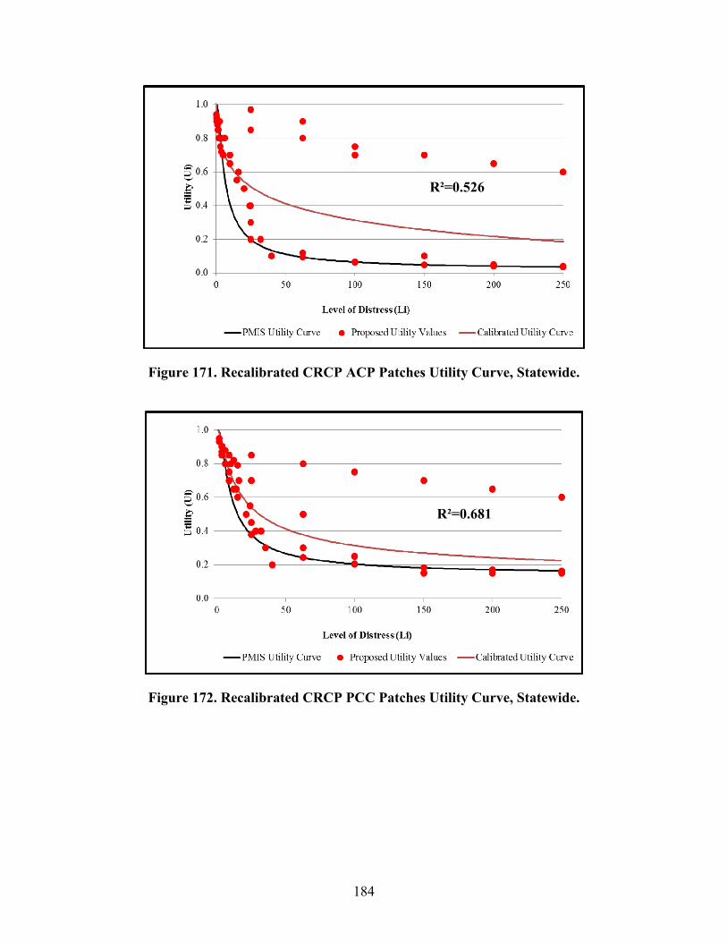
184

Figure 171. Recalibrated CRCP ACP Patches Utility Curve, Statewide.

Figure 172. Recalibrated CRCP PCC Patches Utility Curve, Statewide.

R²=0.526

R²=0.681

185

Figure 173. Recalibrated CRCP Ride Quality Utility Curve for All Traffic Levels, Statewide.

Table 59. R2 Values for Different Traffic Class Values of Ride Score. Ride Score Traffic Class Value of R2

Low 0.793

Medium 0.845

High 0.799

CONCLUSIONS

General observations made from the recalibrated utility curves are:

1. From the recalibrated spalled cracks utility curve, it is observed that presence of less than 76 spalled cracks per mile gives a pavement utility value lower than the utility value given by the current PMIS curves. This can be observed in Figure 169. Given the presence of no other distress or ride quality issue, this can also be interpreted as lower distress and Condition Scores. The opposite behavior is observed for spalled cracks greater than this value.

2. The recalibrated punchouts utility curve is very similar to the current PMIS utility curve. In the presence of more than nine punchouts per mile, the utility represented by the recalibrated curve is larger than the current PMIS curve. This can be observed in Figure 170.

3. The recalibrated ACP and PCC patches utility curves generally give higher utility ratings than their respective current PMIS utility curves. This means that given the presence of no other distress or ride quality issue, we will usually obtain higher Distress and Condition Scores. If extensive patching is present then the Distress and Condition Scores are not penalized as much as with the current PMIS utility curve. However, the greater impact in the

186

calculation of the Distress and Condition Scores is caused when a small number of patches are present as shown by both the current and recalibrated PMIS utility curves.

4. The high traffic level ride quality utility curve recommended for all traffic levels generally gives lower utility values than the current PMIS ride quality utility curves for the low and medium traffic levels. Nevertheless, when only compared to the current high traffic level utility curve, which represents 93 percent of CRCP statewide in 2010, the recalibrated curve is very similar. This concurs with the experts’ opinions about the current ride quality utility curve.

5. Appendix Q contains the impact analysis of these changes to the calculation of distress and Condition Scores for CRCP.

187

CHAPTER 9. PROPOSED CHANGES TO JOINTED CONCRETE PAVEMENT UTILITY CURVES

INTRODUCTION

Utilities are subjective evaluations of the pavements’ ability to carry traffic, measured in a scale from 0 to 1 and calculated according to Eq. 35. U=0 would describe a pavement that can no longer carry traffic and U=1 a new pavement. The utility of a given distress is 1 when the distress level L is zero (no distress leads to maximum utility). As L increases, the utility decreases according to Eq. 35, dropping to a minimum that represents the ability to carry traffic of a pavement with level L of distress type i.

(35) where:

L = level of distress manifestation or ride score loss. e = base of natural logarithms. α, β, and ρ = equation 1 coefficients. Values of original and updated coefficients are tabulated in Appendix M and discussed in the sections titled after each distress manifestation. Distress levels L are used in Eq. 35 as recorded in PMIS for the five JCP distress manifestations previously discussed in this report: failed joints and cracks (FJC), failures (FL), LC, SS, and concrete patches (CP). For the RS utility, L is the ride score loss (RSL) with respect to minimum values corresponding to no utility loss, which are currently defined for three traffic levels as depicted in Table 60. These values are analyzed later, in conjunction with the proposed updates. RSL is calculated according to Eq. 36.

(36) where:

RS = ride score from 0 to 5, as recorded in PMIS. L= RSL = ride score loss. RSmin = see Table 60.

Table 60. Minimum JCP Ride Score Values.

Source: Stampley et al. 1995

188

TxDOT’s PMIS evaluates pavement performance based on two indices that depend on utilities: the DS and the CS. DS and CS are calculated according to Eq. 37 and 38. The DS of a JCP section presenting only one type of distress is 100 times the utility value of that distress level. The CS of a distress-free section is the ride score loss utility times 100.

(37) CS=DS*(RSLu) (38) where:

Subscript “i” = the type of JCP distress manifestation. n = the number of distress manifestations considered in PMIS. Ui = distress utility values between 0 and 1, calculated according to Eq. 35. RSLu = the utility of the ride score loss, calculated with Eqs. 35 and 36. JCP distresses, DS and CS, were described in detail in a previous chapter. DS and CS interpretations are repeated in Table 61 for the readers’ convenience.

Table 61. PMIS Scores Interpretation.

Class Pavement Condition Distress Score Condition Score

A Very Good 90–100 90–100 B Good 80–89 70–89 C Fair 70–79 50–69 D Poor 60–69 35–49 F Very Poor ≤59 1–34

Source: TxDOT, 1997

INTERPRETATION OF UTILITY EQUATION COEFFICIENTS

Coefficient α in Eq. 35 controls the horizontal asymptote of the utility curve. As depicted in Figure 174, [α-1] is the minimum value of the utility, which is not necessarily zero because a distressed pavement may still have some utility (Stampley et al. 1995).

Coefficient β controls the slope of the curve at the inflection point (Figure 175). Coefficient ρ indicates the distress value at the inflection point, as shown in Figure 176 (see also ρ=30 in Figure 175). Distress manifestations considered problematic at relatively low levels can have low values of β as well as ρ, so that the utility drops fast for low distress levels. The utility curve is very sensitive to small changes in β, as depicted in Figure 175.

189

0.0

0.1

0.2

0.3

0.4

0.5

0.6

0.7

0.8

0.9

1.0

0 10 20 30 40 50 60 70 80 90 100 110 120

Utility

Distress Level

α=0.1

α=0.2

α=0.3

α=0.4

α=0.5

α=0.6

α=0.7

α=0.8

α=0.9

α=1

Figure 174. Impact of Coefficient α (ρ=β=1).

0.0

0.1

0.2

0.3

0.4

0.5

0.6

0.7

0.8

0.9

1.0

0 10 20 30 40 50 60 70 80 90 100 110 120

Utility

Distress Level

β=0.5

β=1

β=1.5

β=2

β=2.5

β=3

ρ=30α=1

Figure 175. Impact of Coefficient β.

190

0.0

0.1

0.2

0.3

0.4

0.5

0.6

0.7

0.8

0.9

1.0

0 10 20 30 40 50 60 70 80 90 100 110 120

Utility

Distress Level

ρ=10

ρ=20

ρ=30

ρ=40

ρ=50

ρ=60

Figure 176. Impact of Coefficient ρ.

OBJECTIVES OF THE JCP UTILITY CURVES UPDATE

The original utility curves were developed in the 1990s, and since then TxDOT has accumulated considerable additional experience with them as well as with DS, CS, and their interpretation. As a result, TxDOT decided to have the PMIS utility curves updated to ensure that DS and CS reflect current District needs and practices for each pavement type. The specific objectives of the JCP utility curves updates are to:

Develop different distress utility curves for different traffic levels (JCP distress utilities are currently the same for all traffic levels).

Update the minimum RS values depicted in Table 60 as well as the RSL utility curves to reflect current District practices.

Verify and, if applicable, update DS and CS calculations (Eqs. 37 and 38) to reflect responses to a questionnaire regarding these indices.

The original utility curves are presented in conjunction with the updated ones to facilitate the discussion and enable comparisons between original and updated curves. The coefficients of the updated and original utility curves are tabulated in Appendix M.

METHODOLOGY FOR UPDATING JCP UTILITIES

Traditional utility theory states that utility function points should represent expert opinions on the subject at hand. Opinions are usually elicited through questionnaires and/or surveys designed for this purpose (Inoue et al. 2009).

In this project, JCP utility points were elicited in two phases. In phase 1, a JCP field survey was conducted as part of Subtask 1.5, and its results were used to develop preliminary utility curves.

191

These preliminary curves were submitted to TxDOT’s JCP experts along with a JCP utility questionnaire. In phase 2, the preliminary curves were finalized based on questionnaire responses.

The approach to develop the preliminary curves in phase 1 consisted of the four steps described below.

1. Literature review, especially Lukefahr (2010) and the Beaumont District Plan to Improve Pavement Scores (2008).

2. Statistical analyses of PMIS historical distress levels and of their progression onto the next distress (for example, failures being patched), which indicated how far distresses are allowed to progress and how soon they are treated. Minimum utilities corresponded to distress levels observed at low historical percentiles. This analysis helped define the curves’ horizontal asymptote and its slope magnitude.

3. Analysis of a survey totaling 35 opinions about 13 JCP sections, in which TxDOT experts subjectively evaluated distress levels, CS and DS, and recommended treatments as well as their time frames (how long they could wait). This survey is discussed in detail in a previous chapter. Phase 1 utility function points were estimated as follows: for each survey section and each distress i, distress levels Li were retrieved from PMIS 2011 and matched with the subjective DS and CS estimates from the survey. Elicited utility points for each Li are survey estimates divided by 100 (see Eq. 37).

4. The preliminary utility curves developed in phase 1 defined values of the coefficients α, β, and ρ that made the curve fit as close as possible to the survey points defined in step 3 as well as the horizontal asymptote and the slope boundaries defined in step 2. Given the small size of the survey data, there were limited points for each distress and certainly not sufficient data for fitting separate curves for low, medium, and heavy traffic.

In phase 2, the preliminary utility curves developed in phase 1 were submitted to TxDOT experts along with a questionnaire designed to elicit utility points by traffic level, verify the minimum Ride Score values, and check DS and CS definitions. Two responses were received, which provided utility points in general different than those based on the field survey. The revised curves balance the results of the field survey, the utility questionnaire, and the experts’ comments and recommendations.

UPDATED UTILITY FUNCTIONS

The proposed utility functions are discussed in this section, under headings identifying each distress manifestation. These sections have four figures each. The fourth figure compares the original and the three utility functions proposed for each traffic level (i.e., low, medium, and heavy). The first three compare the five characteristics identified below:

1. The original utility function (which is the same for all traffic levels except in the case of Ride Score loss).

192

2. The points from the field survey.

3. The preliminary curve fitted to the field survey results during phase 1.

4. The points elicited with phase 2 questionnaire (there were two responses).

5. The updated curve, fitted through questionnaire points and survey points, and also reflecting TxDOT’s comments and suggestions from the questionnaire when applicable.

The concluding section of this chapter presents the combined impact of the updated functions on the evaluation of the JCP network, comparing the percent of JCP sections classified into the categories depicted in Table 61 (poor, fair, etc.), with the original and updated utility functions.

Failed Joints and Cracks (FJC)

Figures 177–179 depict the updated curves for low, medium, and heavy traffic, respectively. Figure 180 compares the three updated functions to the original function. Some questionnaire responses indicated significantly lower utilities for high FJC values, as indicated in the three figures. These responses clearly deviate from the sigmoidal format of Eq. 35. However, the parts of these curves corresponding to high FJC levels are theoretical; untreated FJCs would progress into failures.

The updated low traffic function slightly increases the utilities with respect to the original, while the heavy traffic function decreases it. For medium traffic, the utilities are approximately the same as the original up to FJC≈30 percent; after that, they decrease with respect to the original function.

0.0

0.1

0.2

0.3

0.4

0.5

0.6

0.7

0.8

0.9

1.0

0 10 20 30 40 50 60 70 80 90 100

FJC Utility, Low Traffic

FJC (% )

Original

Preliminary (Phase 1)

Proposed (Phase 2)

Field Survey

Questionnaire Response 1


Figure 177. Updated Low Traffic Utility Function for

Failed Joints and Cracks.

193

0.0

0.1

0.2

0.3

0.4

0.5

0.6

0.7

0.8

0.9

1.0

0 10 20 30 40 50 60 70 80 90 100

FJC Utility, M

edium Traffic

FJC (% )

Original


Proposed (Phase 2)

Field Survey



Figure 178. Updated Medium Traffic Utility Function for


0.0

0.1

0.2

0.3

0.4

0.5

0.6

0.7

0.8

0.9

1.0

0 10 20 30 40 50 60 70 80 90 100

FJC Utility, H

eavy Traffic

FJC (% )

Original


Proposed (Phase 2)

Field Survey



Figure 179. Updated Heavy Traffic Utility Function for


194

0.0

0.1

0.2

0.3

0.4

0.5

0.6

0.7

0.8

0.9

1.0

0 10 20 30 40 50 60 70 80 90 100

FJC Utility

Failed Joints and Cracks (%)

OriginalLow TrafficMedium TrafficHeavy Traffic

Figure 180. Updated Utility Functions for Failed Joints

and Cracks, Comparison.

The impact of using the updated FJC utility functions instead of the original one on the DS of a section where only failed joints and cracks are present can be illustrated by comparing the FJC levels required to reach DS=69, the upper threshold of a “poor” JCP (see Table 61). These levels are:

FJC = 40 percent for all traffic levels with the original utility function. FJC = 54 percent with the utility function updated for low traffic. FJC = 35.5 percent with the utility function updated for medium traffic. FJC = 26.6 percent with the utility function updated for heavy traffic.

Failures (F)

Figures 181–183 depict the updated curves for low, medium, and heavy traffic, respectively. The parts of these curves beyond 50 failures/mile would be used very rarely, since more than 99 percent of the records in the 13-year PMIS database are below this value. The historical maximum is 125 failures/mile. Figure 184 presents a comparison among the three updated curves and the original one.

195

0.0

0.1

0.2

0.3

0.4

0.5

0.6

0.7

0.8

0.9

1.0

0 10 20 30 40 50 60 70 80 90 100 110 120

Failures Utility, Low Traffic

Failures/mile

Original


Proposed (Phase 2)

Field Survey



Figure 181. Updated Low Traffic Utility Function for Failures.

0.0

0.1

0.2

0.3

0.4

0.5

0.6

0.7

0.8

0.9

1.0

0 10 20 30 40 50 60 70 80 90 100 110 120

Failures Utility, M

edium Traffic

Failures/mile

Original


Proposed (Phase 2)

Field Survey



Figure 182. Updated Medium Traffic Utility Function for Failures.

196

0.0

0.1

0.2

0.3

0.4

0.5

0.6

0.7

0.8

0.9

1.0

0 10 20 30 40 50 60 70 80 90 100 110 120

Failures Utility, H

eavy Traffic

Failures/mile

Original


Proposed (Phase 2)

Field Survey



Figure 183. Updated Heavy Traffic Utility Function for Failures.

0.0

0.1

0.2

0.3

0.4

0.5

0.6

0.7

0.8

0.9

1.0

0 10 20 30 40 50 60 70 80 90 100 110 120 130

Failures Utility

Failures/mile

Original

Low Traffic

Medium Traffic

Heavy Traffic

Figure 184. Updated Utility Functions for Failures: Comparison.

Both questionnaire responses were consistent in recommending higher utilities than the original values for all traffic levels, but one response recommended significantly higher utilities than all other available evaluations (i.e., original utility curve, the preliminary curve developed in phase 1, and the other questionnaire response). It would be interesting to elicit additional failures utilities from different experts in order to further refine the failures utility curves.

The impact of using the updated utility functions instead of the original one on the DS of a section where only failures are present can be illustrated by comparing the number of failures

197

required to reach DS=69, which is the upper threshold of a “poor” JCP (see Table 61). These levels are:

F = 14.3/mile for all traffic levels with the original utility function. F = 26.1/mile with the utility function updated for low traffic. F = 23.4/mile with the utility function updated for medium traffic. F = 18.5/mile with the utility function updated for heavy traffic.

Concrete Patches (CP)

As discussed in the Beaumont District Plan to Improve Pavement Scores (2008), “nine concrete patches per half mile on JCP gives DS=72,” and “anytime the number of patches approached these numbers, the pavement had to have a new surface, even if there were no other distress or ride problems.”

While the number of patches is important to make treatment decisions and should be part of PMIS scores, it does not seem cost-effective to assign a low DS and therefore recommend treatments to properly patched JCP sections with few or no other distresses. The questionnaire responses seemed to agree with this underlying notion, which is reflected in the updated curves. Most questionnaire responses increased the utility values of a patched JCP with respect to both the original and the preliminary (phase 1) curves.

Figures 185–187 depict the updated patches utility curves for low, medium, and heavy traffic, respectively. Figure 188 presents a comparison among the three updated curves and the original one.

The parts of these utility curves beyond 55 patches/mile would be rarely used, since more than 95 percent of the records in the 13-year PMIS database are below this value. The historical maximum is 200 patches/mile.

198

0.0

0.1

0.2

0.3

0.4

0.5

0.6

0.7

0.8

0.9

1.0

0 20 40 60 80 100 120 140 160 180 200

P Utility, Low Traffic

Patches / mile

OriginalPreliminary (Phase 1)Proposed (Phase 2)Field SurveyQuestionnaire Response 1Questionnaire Response 2

Figure 185. Updated Low Traffic Utility Function for Concrete Patches.

0.0

0.1

0.2

0.3

0.4

0.5

0.6

0.7

0.8

0.9

1.0

0 20 40 60 80 100 120 140 160 180 200

P Utility, M

edium Traffic

Patches / mile

Original


Proposed (Phase 2)

Field Survey



Figure 186. Updated Medium Traffic Utility Function for Concrete Patches.

199

0.0

0.1

0.2

0.3

0.4

0.5

0.6

0.7

0.8

0.9

1.0

0 20 40 60 80 100 120 140 160 180 200

P Utility, H

eavy Traffic

Patches / mile

Original


Proposed (Phase 2)

Field Survey



Figure 187. Updated Heavy Traffic Utility Function for Concrete Patches.

0.0

0.1

0.2

0.3

0.4

0.5

0.6

0.7

0.8

0.9

1.0

0 10 20 30 40 50 60 70 80 90 100

Patches Utility

Patches / mile


Figure 188. Updated Utility Functions for Concrete Patches: Comparison.

The impact of using the updated utility functions instead of the original one on the DS of a section where only concrete patches are present can be illustrated by comparing the patches’ levels required to reach DS=69, the upper threshold of a “poor” JCP (see Table 61). These levels are:

P = 19.6/mile for all traffic levels with the original utility function. P = 61.5/mile with the utility function updated for low traffic.

200

P = 50.0/mile with the utility function updated for low traffic. P = 36.5/mile with the utility function updated for heavy traffic.

Longitudinal Cracks

Figures 189–191 depict the updated LC utility curves for low, medium, and heavy traffic, respectively. Figure 192 presents a comparison among the three updated curves and the original one.

The parts of these curves beyond LC=6 percent would be rarely used, since more than 95 percent of the records in the 13-year PMIS database are less than this value. Moreover, 85 percent of the sections have LC=0. The historical maximum is 96.6 percent.

One of the two questionnaire response assigned higher utilities than the original, while the other assigned lower utilities. In this case, additional questionnaire responses would have been particularly beneficial.

0.0

0.1

0.2

0.3

0.4

0.5

0.6

0.7

0.8

0.9

1.0

0 10 20 30 40 50 60 70 80 90 100

LC Utility, Low Traffic

Longitudinal Cracks (% slabs)

Original


Proposed (Phase 2)

Field Survey



Figure 189. Updated Low Traffic Utility Function for Longitudinal Cracks.

201

0.0

0.1

0.2

0.3

0.4

0.5

0.6

0.7

0.8

0.9

1.0

0 10 20 30 40 50 60 70 80 90 100

LC Utility, M

edium Traffic


Original


Proposed (Phase 2)

Field Survey



Figure 190. Updated Medium Traffic Utility Function for Longitudinal Cracks.

0.0

0.1

0.2

0.3

0.4

0.5

0.6

0.7

0.8

0.9

1.0

0 10 20 30 40 50 60 70 80 90 100

LC Utility, H

eavy Traffic


Original


Proposed (Phase 2)

Field Survey



Figure 191. Updated Heavy Traffic Utility Function for Longitudinal Cracks.

202

0.0

0.1

0.2

0.3

0.4

0.5

0.6

0.7

0.8

0.9

1.0

0 10 20 30 40 50 60 70 80 90 100

LC U

tility

Longitudinal cracks (% slabs)


Figure 192. Updated Utility Functions for Longitudinal Cracks: Comparison.

The impact of using the updated utility functions on the DS of a section where only longitudinal cracks are present can be illustrated by comparing the LC levels required to reach DS=69, the upper threshold of a “poor” JCP (see Table 61). These levels are listed below, but they can be viewed as theoretical, given the fact that 95 percent of all sections in the historical data base have LC below 6 percent.

LC = 40.5 percent for all traffic levels with the original utility function. LC = 43 percent with the utility function updated for low traffic. LC = 31 percent with the utility function updated for medium traffic. LC = 24 percent with the utility function updated for heavy traffic.

Shattered Slabs

Figures 193–Figure 195 depict the updated SS utility curves for low, medium, and heavy traffic, respectively. Figure 196 presents a comparison among the three updated curves and the original one. Only the beginning of these curves is relevant in practical terms, because over 99 percent of the records indicate SS<1. The historical maximum is 30.3 percent.

Shattered slabs are present in only 2.5 percent of the entire historical JCP database. In other words, they are repaired as soon as they appear, and/or other distresses are treated before they progress into shattered slabs. The preliminary curve (phase 1, depicted in green in Figures 193–195) reflected this practice by assigning utilities that would make the “fair” pavement threshold of DS=70 to be reached when SS approaches 1 percent. However, the questionnaire responses assigned the “fair” threshold to much higher levels of this distress, while lowering the utility values with respect to the original for the beginning of the curves. Given this difference, it was decided to update the utilities based primarily on the questionnaire. The practical impact of changing SS utility curves is negligible on the network-level evaluation, due to rare occurrence of this distress.

203

0.0

0.1

0.2

0.3

0.4

0.5

0.6

0.7

0.8

0.9

1.0

0 10 20 30 40 50 60 70 80 90 100

SS Utility, Low Traffic

Shattered Slabs (%)

Original


Proposed (Phase 2)

Field Survey



Figure 193. Updated Low Traffic Utility Function for Shattered Slabs.

0.0

0.1

0.2

0.3

0.4

0.5

0.6

0.7

0.8

0.9

1.0

0 10 20 30 40 50 60 70 80 90 100

SS Utility, M

edium Traffic

Shattered Slabs (%)

Original


Proposed (Phase 2)

Field Survey



Figure 194. Updated Medium Traffic Utility Function for Shattered Slabs.

204

0.0

0.1

0.2

0.3

0.4

0.5

0.6

0.7

0.8

0.9

1.0

0 10 20 30 40 50 60 70 80 90 100

SS Utility, H

eavy Traffic

Shattered Slabs (%)

Original


Proposed (Phase 2)

Field Survey



Figure 195. Updated Heavy Traffic Utility Function for Shattered Slabs.

0.0

0.1

0.2

0.3

0.4

0.5

0.6

0.7

0.8

0.9

1.0

0 10 20 30 40 50 60 70 80 90 100

SS Utility

Shattered Slabs (%)

Original

Low Traffic

Medium Traffic

Heavy Traffic

Figure 196. Updated Utility Functions for Shattered Slabs: Comparison.

Ride Score Loss

Characteristics of JCP Ride Scores

The Ride Score is not a particularly well-suited indicator of JCP performance, since it changes little from year to year and from one section to another. Historically, Ride Scores have been statistically the same for medium and low traffic sections and higher (rather than lower) for heavy traffic sections. A non-parametric test of RS difference between medium and low traffic

205

turned out to be non-significant (P-value=0.06). Heavy traffic section Ride Scores, on the other hand, were significantly greater than the RS of the pooled medium and low traffic sections (P-value<0.001).

Figure 197 depicts the cumulative distribution of Ride Scores observed in the historical database. It helps visualize the similarity of low and medium traffic Ride Scores and the consistently higher Ride Scores in heavy traffic sections. In Figure 197, the cumulative distributions of medium and low traffic (i.e., yellow and green curves) are intertwined, while the heavy traffic distribution sits below the other two.

0

10

20

30

40

50

60

70

80

90

100

0 1 2 3 4 5

Cumulative Percentile

Ride Score

Heavy Traffic

Medium Traffic

Low Traffic

Figure 197. Cumulative Ride Score Percentiles in the Historical JCP Database.

The historical mean RS is 2.7 for medium/low and 2.9 for heavy traffic. The 99 percent confidence interval for the difference between heavy traffic Ride Scores (RSH) and low/medium (RSM/L) is [+0.2114 0.0022]. On the average, RSH=RSM/L+0.2 at 99 percent confidence. The data strongly suggest that JCP Ride Scores reflect stricter construction and maintenance practices in heavy traffic sections, which are intended to compensate for the additional wear-and-tear.

Additional statistical analyses of the 13-year historical database indicated that the RS tends to remain constant with time, as opposed to JCP distresses, which tend to increase during the periods when they remain untreated. As discussed in the chapter on JCP performance prediction models, three goodness-of-fit tests indicated that JCP Ride Scores are normally distributed. Ride scores were not significantly different by JCP type (P-value>0.08) thus confirming the original assumption (the original RS utilities are the same for both JCP types).

Minimum Ride Score Values for No Utility Loss

As already explained in the “Background and Objective” section, PMIS defines a “minimum” RS value above which there is no utility loss (U=1). Ride score utilities are defined in terms of the percent Ride Score loss (RSL) with respect those minima (see Eq. 36). The original minima (see Table 60) are 2.5, 3.0, and 3.5, respectively, for low, medium, and heavy traffic (Stampley

206

et al. 1995). The utility questionnaire obtained the following two responses for the cut-off value above which there should be no utility loss (and therefore no Ride Score loss either):

5/4.5 for heavy traffic. 5/4.0 for medium traffic. 5/3.5 for low traffic.

The 13-year PMIS database was used to verify whether or not these minima (original and proposed by respondents) actually reflect District practices and the realities of JCP ride quality. Table 62 depicts RS occurrences at or above the RS minimum values listed above in the 13-year database.

Table 62. Historical Frequencies of Sections by Ride Score Range. Minimum RS for U=1 Historical Occurrence RS=5.0 for all traffic levels: 3 heavy traffic sections

Questionnaire RS≥4.5 for heavy traffic: 152 sections (0.51%) Responses RS≥4.0 for medium traffic: 53 sections (0.18%)

RS≥3.5 for low traffic: 182 sections (0.61%) RS≥3.5 for heavy traffic: 4,331 sections (17.7%)

Original values RS≥3.0 for medium traffic: 1,031 sections (30.9%) RS≥2.5 for low traffic: 1,432 sections (68.5%)

Using the original RS utility function and minimum values, CS=100 occurred in 5909 of the 6794 sections with RS greater than the original RSmin for each traffic level. These 5909 sections correspond to approximately 20 percent of all JCP sections in the historical database. The proposed minimum value of RS=5.0 for all traffic level resulted in a mere three sections with a perfect Condition Score. The other questionnaire response (4.5, 4.0, and 3.5) resulted in less than 0.5 percent sections with CS=100.

Neither response contributes to more realistic JCP Condition Scores, but both respondents advised increasing the minimum values corresponding to U=1, and their practical experience is very valuable for this project. The updated minima are between the original values and the values recommended by the two respondents and correspond to 7 percent of the sections in both categories, ensuring uniform criteria. The updated minima are:

RS≥4.0 for heavy traffic (7 percent). RS≥3.6 for medium & low (7 percent).

Updated Ride Score Loss (RSL) Utilities

Figure 198 depicts the two questionnaire responses as asked, i.e., as a function of Ride Score rather than RSL, since the minima were also under investigation. The red and blue rectangles indicate the regions where RSL=0, respectively, for heavy and low/medium traffic, with RSL calculated according to Eq. 36 using the updated minima. When plotted against RSL rather than RS, the responses falling inside these rectangles line up with RSL=0. The best fit to the responses and the updated minimum RS values would require changing Eq. 35 into Eq. 39,

207

where “y” would be the lowest RS utility the respondents assigned to RS values above the updated minima, since they are lower than the minima proposed by the respondents.

(35) into:

(39)

0

0.1

0.2

0.3

0.4

0.5

0.6

0.7

0.8

0.9

1

012345

Elicited Utility

Ride Score

Respondent 1Respondent 2HeavyMediumLow

Proposed RS Loss=0 (heavy traffic)

Proposed RS Loss=0 (medium and low traffic)

Figure 198. Questionnaire Responses and Updated Region of RSL=0.

This equation change is not recommended since it conflicts with the definition of minimum RS with no utility loss. The updated utilities in effect recalibrated Eq. 35 coefficients through the two questionnaire responses obtained, using the updated minimum RS values to calculate RSL. Figures 199 and 200 depict the original and updated RSL utility curves and the questionnaire responses, respectively, for heavy traffic and for low/medium traffic in both figures. One response is represented as a triangle and the other as a circle with both color-coded by traffic level as indicated in the legend. Figure 201 depicts a comparison among the original and updated functions.

In all figures, the RSL was calculated according to Eq. 35, using the original minimum values for the original curves, and the updated minima for the updated curves and questionnaire responses. The parts of the curves corresponding to questionnaire responses above the updated RS minimum values were kept as close as possible to the original.

The original curves reach the point of U=0 for high RSL values. However, it is impossible to fit a sigmoidal curve that passes through all questionnaire responses and also through the point [100,0], i.e., the point matching zero utility to total Ride Score loss. For practical purposes, however, only the values corresponding to RSL≤50 percent are relevant, because

208

RSL≥50 percent with respect to updated minima occurs in only 1.3 percent of the sections in the historical database. For heavy traffic, the best fit to the questionnaire responses is the straight line indicated in Figure 199. However, utilities are defined as asymptotic functions, so a straight line is not recommended.

0

0.1

0.2

0.3

0.4

0.5

0.6

0.7

0.8

0.9

1

0 10 20 30 40 50 60 70 80 90 100

Heavy Traffic RS Utility

Ride Score Loss (%)

Questionnaire Response 1Questionnaire Response 2Original Equation and Minimum RSProposed Equation and Minimum RSBest Fit: RSu=1‐0.0072*RSL

Figure 199. Ride Score Loss Utility for Heavy Traffic.

209

0.0

0.1

0.2

0.3

0.4

0.5

0.6

0.7

0.8

0.9

1.0

0 10 20 30 40 50 60 70 80 90 100

Low &Medium Traffic RS Utility

Ride Score Loss (%)

Questionnaire Response 1 (Low)

Questionnaire Response 2 (Low)

Original Equation and Minimum RS (Low Traffic )

Questionnaire Response 1 (Medium)

Questionnaire Response 2 (Medium)

Original Equation and Minimum RS (Medium Traffic)

Proposed Equation and Minimum RS (L&M)

Figure 200. Ride Score Loss Utility for Medium and Low Traffic.

0.0

0.1

0.2

0.3

0.4

0.5

0.6

0.7

0.8

0.9

1.0

0 10 20 30 40 50 60 70 80 90 100

Ride Score Utility

Ride Score Loss (%)

Proposed, Heavy Traffic

Proposed, Low & Medium Traffic

Original Equation and Minimum RS (Heavy Traffic)

Original Equation and Minimum RS (Medium Traffic)

Original Equation and Minimum RS (Low Traffic )

Figure 201. Updated and Original Utility Functions for Ride Score Loss.

210

PMIS SCORES CALCULATIONS

The questionnaire responses regarding the PMIS score calculations depicted in Eqs. 37 and 38 indicated that the Ride Score should have less importance than the Distress Score in the JCP Condition Score calculation. Table 63 depicts both responses and their average.

The updated utilities are greater than the originals and already decrease the Ride Score importance in the CS calculation. Therefore, no changes are proposed to the distress and Condition Score formulas.

Table 63. Ride Score Importance to the Condition Score Calculation. Traffic Relevance to CS calculations Level Distress Score Ride Score

Response 1 Heavy 44% 56% Medium 45% 55%

Low 46% 54% Response 2 Heavy 60% 40%

Medium 70% 30% Low 80% 20%

Average Heavy 52% 48% Medium 57% 43%

Low 63% 37%

IMPACTS, CONCLUSIONS, AND RECOMMENDATIONS

The updated distress utilities had the following general impact on the scores of the 3,522 JCP sections in PMIS 2011 database (data from PMIS tables “PMIS JCP Ratings” and “PMIS Scores Summary”):

The average Distress Score of JCP sections increased from 82 to 87.

No significant change in the average Distress Score of JCP sections presenting only failed joints and cracks (decreased by 0.3).

Slight increase in the average Distress Score of JCP sections presenting only failures (changed from 93 to 95).

Considerable improvement in the Distress Score of properly patched JCPs with no other problems. The average Distress Score of sections presenting only patches increased from 81.0 to 90.7.

No significant change in the Distress Score of sections presenting only longitudinal cracks (LC) (average Distress Score decreased by 0.6).

Significant improvement in the overall average Condition Score: it increased from 65.8 (poor) to 76.2 (good).

211

The average Condition Score of sections presenting only failed joints and cracks improved from 80.0 to 87.1.

The average Condition Score increased from 60.1 to 76.5 in sections presenting only patches, and from 86.4 to89.2 in sections presenting only longitudinal cracks.

Appendix S presents a detailed impact analysis of the proposed changes on the PMIS 2011 utility functions used to calculate the PMIS scores.

213

CHAPTER 10. PROPOSED CHANGES TO ASPHALT CONCRETE PAVEMENT DECISION TREES

INTRODUCTION

Currently, TxDOT’s PMIS ACP needs estimate procedure suggests broad treatment types based on distress, ride, ADT levels, and age information stored in PMIS. Tables 64 and 65 are summaries of the ACP reason codes in PMIS. The trigger criteria listed in those tables are used in the PMIS decision tree for ACP. The actual decision tree is too large to be reproduced in this report.

Table 64. PMIS Needs Estimate Trigger Criteria for Rehabilitation Treatment Recommendations.

PMIS Needs Estimate Reason Code Pavement Treatment Code Needs Estimate Trigger Criterion

A005 Heavy Rehab ADT per lane greater than 5,000 and Ride Score less than 2.5

A010 Heavy Rehab ADT per lane greater than 750 and Ride Score less than 2.0A015 Heavy Rehab Ride Score less than 1.5A020 Heavy Rehab Deep Rutting greater than 50 percent

A025 Heavy RehabADT per lane greater than 750 and Ride Score less than 3.0 and Alligator Cracking greater than 50 percent

A030 Heavy RehabRide Score less than 2.5 and Alligator Cracking greater than 50 percent

A100 Medium Rehab ADT per lane greater than 5,000 and Ride Score less than 3.0

A105 Medium Rehab ADT per lane greater than 750 and Ride Score less than 2.5A110 Medium Rehab Ride Score less than 2.0

A115 Medium RehabADT per lane greater than 750 and Deep Rutting greater than 25 percent

A120 Medium Rehab Alligator Cracking greater than 50 percent

A125 Medium RehabADT per lane greater than 5,000 and Alligator Cracking greater than 10 percent

A130 Medium Rehab Failures greater than or equal to 10 per mile

A135 Medium RehabADT per lane greater than 750 and Failures greater than or equal to 5 per mile

A140 Medium RehabADT per lane greater than 750 and Block Cracking greater than 50 percent

A200 Light Rehab Ride Score less than 2.5

A300 Light RehabADT per lane to "High" based on Functional Class and Shallow Rutting greater than 25 percent

A305 Light RehabADT per lane to "High" based on Functional Class and Deep Rutting greater than 10 percent

A310 Light RehabADT per lane to "High" based on Functional Class and Ride Score less than 3.0

214

Table 65. PMIS Needs Estimate Trigger Criteria for Preventive Maintenance Recommendations.

PMIS Needs Estimate Reason Code Pavement Treatment Code Needs Estimate Trigger Criterion

A400 Preventive MaintenanceADT per lane to "Low" based on Functional Class and Shallow Rutting greater than 50 percent

A405 Preventive MaintenanceADT per lane to "Low" based on Functional Class and Deep Rutting greater than 10 percent

A500 Preventive MaintenanceADT per lane to "High" based on Functional Class and Block Cracking greater than 5 percent

A505 Preventive MaintenanceADT per lane to "High" based on Functional Class and Failures greater than 1 per mile

A510 Preventive MaintenanceADT per lane to "High" based on Functional Class and Alligator Cracking greater than 5 percent

A515 Preventive MaintenanceADT per lane to "High" based on Functional Class and Longitudinal Cracking greater than 50 feet per station

A520 Preventive MaintenanceADT per lane to "High" based on Functional Class and Transverse Cracking greater than 2 per station

A600 Preventive MaintenanceADT per lane to "Low" based on Functional Class and Alligator Cracking greater than 5 percent

A605 Preventive MaintenanceADT per lane to "Low" based on Functional Class and Block Cracking greater than 5 percent

A610 Preventive MaintenanceADT per lane to "Low" based on Functional Class and Failures greater than 1 per mile

A615 Preventive MaintenanceADT per lane to "Low" based on Functional Class and Longitudinal Cracking greater than 50 feet per station

A620 Preventive MaintenanceADT per lane to "Low" based on Functional Class andTransverse Cracking greater than 2 per station

A700 Preventive Maintenance Shallow Rutting greater than 25 percentA705 Preventive Maintenance Deep Rutting greater than 0 percentA900 Preventive Maintenance Age of last surface greater than 7 years

Researchers evaluated the trigger criteria based on the data comparisons and interviews described in Chapter 3, analyzed PMIS data, and used the information and results described in Mr. Charles Gurganus’ thesis, which is included in this report as Appendix W. This chapter documents further analysis of the data and recommendations for changing the ACP decision tree needs estimate trigger criteria.

DEEP RUTTING CRITERIA

When evaluating the Beaumont, Bryan, and Dallas District Needs Estimates, researchers discovered drastic swings in the percent of Needs Nothing sections. Table 66 below illustrates the percent of NN sections for these three Districts from FY 2004 through FY 2009.

215

Table 66. Percent of NN Sections for Bryan, Beaumont, and Dallas.

FY %NN %PM %LRhb %MRhb %HRhb %NN %PM %LRhb %MRhb %HRhb

2004 66.16% 19.63% 8.36% 4.67% 1.18% 66.17% 19.86% 8.41% 4.59% 0.97%

2005 55.36% 26.60% 10.41% 6.34% 1.30% 55.37% 26.92% 10.44% 6.27% 1.00%

2006 57.96% 22.91% 11.17% 6.56% 1.40% 57.93% 23.02% 11.21% 6.44% 1.41%

2007 60.99% 22.32% 9.42% 5.71% 1.55% 61.09% 22.52% 9.48% 5.57% 1.34%

2008 42.43% 42.57% 8.72% 4.44% 1.84% 42.30% 42.93% 8.74% 4.39% 1.63%

2009 73.02% 12.19% 8.80% 4.66% 1.33% 73.08% 12.34% 8.88% 4.59% 1.10%


2004 56.87% 30.59% 2.86% 6.37% 3.31% 57.72% 35.60% 2.02% 3.33% 1.34%

2005 57.03% 27.27% 3.58% 8.81% 3.31% 58.96% 31.82% 2.78% 5.22% 1.23%

2006 63.94% 22.13% 3.15% 7.62% 3.15% 65.99% 25.66% 2.54% 4.20% 1.61%

2007 63.10% 26.15% 2.58% 5.38% 2.79% 64.82% 30.16% 1.27% 2.64% 1.11%

2008 63.30% 25.65% 3.26% 5.63% 2.17% 64.39% 29.37% 2.17% 3.34% 0.73%

2009 68.72% 19.72% 4.86% 5.69% 1.00% 69.38% 23.13% 3.76% 3.19% 0.54%


2004 52.04% 18.56% 11.49% 14.58% 3.32% 52.59% 25.60% 8.08% 11.43% 2.30%

2005 57.81% 13.70% 10.22% 14.11% 4.17% 61.13% 18.86% 6.99% 10.35% 2.67%

2006 51.66% 13.41% 10.72% 18.50% 5.70% 54.28% 18.95% 9.01% 13.23% 4.53%

2007 45.23% 22.69% 9.80% 17.14% 5.15% 43.74% 31.45% 7.63% 13.09% 4.10%

2008 40.10% 20.79% 10.77% 21.13% 7.21% 40.37% 29.10% 10.18% 14.07% 6.27%

2009 53.66% 14.16% 9.55% 16.83% 5.80% 56.97% 18.47% 8.55% 11.15% 4.85%

Dallas District

Total Asphalt Pavements

Bryan District


Beaumont District


The table above clearly illustrates drastic drops in the quantity of NN sections for the Bryan District in FY 2008 and for the Dallas District in FY 2007 and FY 2008. For Bryan, the change from FY 2007 to FY 2008 is almost 20 percent, while the subsequent increase from FY 2008 to FY 2009 is over 30 percent. Dallas experienced a similar decline in NN sections (this includes sections that have reason code A900) from FY 2006 to FY 2007 where the drop was over 10 percent. While it remains steady through FY 2008, there has been a rise of almost 17 percent from FY 2008 to FY 2009. Additional investigation proved that reason code A705 (PM for deep rutting greater than 25 percent) is the major culprit for the drastic swings in percent NN sections. Many of these cases add “false” rut values caused by signal scatter when the acoustic rut sensor is measuring a high surface texture pavement (such as a new Grade 3 seal coat). The information from the table above and the aforementioned drastic movements are graphically illustrated in Figures 202 and 203 below.

216

Figure 202. Percent of Sections with NN Reason Codes All Pavement Types.

Figure 203. Percent of Sections with NN Reason Codes for Only Asphalt Pavement Types.

The impact of A705 is shown in Figure 204 below.

217

Figure 204. Sections with A705 Reason Code.

The Bryan District curve clearly indicates multiple drastic shifts in the quantity of A705, although none were larger than the quantity reached in FY 2008. The Dallas District curve is more constant with the exception of FY 2007 and FY 2008 where the quantity of A705 sections rises to above 1000 in each year.

The current description of A705 is “Deep Rutting greater than zero percent,” returning an M&R treatment suggestion of PM. The “zero percent” limit on Deep Rutting was defined in the early 1990s when Rut was rated visually and when Deep Rutting was defined as 1-3 inches. In FY 1996 TxDOT changed to automated acoustic rut sensors; and in FY 2001 the current definition of Deep Rutting, ¼- to ½-inch, was established. However, field observations showed that the acoustic sensors are not accurate enough to measure ½-inch ruts with any kind of confidence, which led to much of the false classifications of reason code A705.

In addition to the redundancy in the reason codes, another reason to rewrite or eliminate A705 is the fact that it uses a 0 percent limit when the utility curves allow a certain percent of deep rutting to accrue before the Distress Score is impacted. Figure 205 below is a screenshot illustrating the current utility curve for deep rutting and pavement type 5.

218

Figure 205. Current Deep Rutting Utility Curve from PMIS.

Based on this utility curve, if A705 is rewritten rather than eliminated, the percent of deep rutting triggering a PM suggestion should coincide with the percent of deep rutting that begins to affect the Distress Score. A405 cannot be eliminated because it has additional ADT/Lane and Functional Class criteria.

FUNCTIONAL CLASS CRITERIA

The current PMIS ACP needs estimate recommendations use actual ADT numbers as the trigger criteria for Medium and Heavy Rehabilitation recommendations. However, for Light Rehabilitation and Preventive Maintenance recommendations, the trigger criteria are a combination of functional class and whether or not the ADT is high or low based on that functional class. Based on interviews conducted with the Districts, TxDOT personnel did not use Functional Class as a factor in determining the type of pavement treatment to be applied. Thus, the researchers generated new decision tree trigger criteria that eliminated functional class and instead used ADT ranges. The recommended ranges indicated later in this chapter are based on ADT ranges that TxDOT staff considered for a multi tier system concept.

219

ADT, DISTRESS QUANTITIES, AND RIDE QUALITY

The District interviews indicated that ADT did play a factor in determining how much distress would be tolerated before a treatment is applied. In other words, District personnel would allow a higher distress level to be present on a lower ADT roadway than a higher ADT roadway before applying a treatment. In addition, District personnel may also allow ride quality to deteriorate to a greater degree on a lower ADT roadway before applying a treatment. Researchers then concluded that the distress and ride quality trigger criteria in the needs estimate should be a function of ADT.

PMIS DATA ANALYSIS

Researchers also analyzed the data in PMIS to determine distributions of individual distress ratings. For the FY 2011 PMIS data, the researchers found the following distress frequency for 174,165 sections, as shown in Tables 67–74.

Table 67. FY 2011 PMIS–Failures.

Failures (no.) No. Obs.

Percent of Total

0 165,127 94.81

1 5,973 3.43

2 1,656 0.95

3 666 0.38

4 293 0.17

5 135 0.08

6 90 0.05

7 54 0.03

>7 171 0.10

220

Table 68. FY 2011 PMIS–Alligator Cracking. Alligator Cracking,

% No. Obs. Percent of Total

0 144,341 82.88

1 7,490 4.30

2 6,439 3.70

3 2,924 1.68

4 2,042 1.17

5 1,501 0.86

6 1,210 0.69

7 821 0.47

8 938 0.54

9 630 0.36

10 385 0.22

>10 5,444 3.13

Table 69. FY 2011 PMIS–Block Cracking. Block

Cracking, % No. Obs.

Percent of Total

0 172,932 99.29

1–4 371 0.21

5–12 276 0.16

13–20 132 0.08

21–27 73 0.04

>27 381 0.22

Table 70. FY 2011 PMIS–Longitudinal Cracking.

Longitudinal Cracking,

ft/sta. No.

Obs. Percent of Total

0 101,893 58.50

1–25 47,710 27.39

26–100 19,035 10.93

101–150 3,563 2.05

151–175 993 0.57

>175 971 0.56

221

Table 71. FY 2011 PMIS–Distribution of Transverse Cracks. Transverse

Cracks (no.) No. Obs.

Percent of Total

0 153,783 88.30

1 9,124 5.24

2 4,714 2.71

3 2,627 1.51

4 1,590 0.91

5 1,045 0.60

6 570 0.33

7 318 0.18

8 147 0.08

>8 247 0.14

Table 72. FY 2011 PMIS–Patching.

Patching, % No. Obs.

Percent of Total

0 146,308 84.01

1–3 6,172 3.54

4–11 9,073 5.21

12–22 5,378 3.09

23–44 4,207 2.42

>44 3,027 1.74

Table 73. FY 2011 PMIS–Deep Rutting.

Deep Rutting, % No. Obs.

Percent of Total

0 156,863 90.07

1–4 15,845 9.10

5–7 864 0.50

8–9 233 0.13

10–11 119 0.07

>11 241 0.14

222

Table 74. FY 2011 PMIS–Shallow Rutting.

Shallow Rutting, % No. Obs.

Percent of Total

0 107,567 61.76

1–5 56,338 32.35

6–9 6,534 3.75

10–13 2,218 1.27

14–18 947 0.54

>18 561 0.32

RECOMMENDED ACP DECISION TREE TRIGGER CRITERIA

Based on the District interviews and analysis of PMIS data, Gurganus and Wimsatt generated the recommended ACP decision tree trigger criteria. Tables 75–78 below have criteria based on ADT levels below 100; between 100 and 1000; between 1000 and 5000; and 5000 or greater. The four tables below have values based on a PMIS section length of 0.5 miles. Note that the tables result in needs estimate suggestions that are based on one distress or ride quality range. Obviously, a section may have several different distresses, but the trigger will be based on the distress that generates the highest needs estimate suggestion.

Table 75. Needs Estimate Trigger Criteria for ADT from 0 to 99. Needs Estimate Suggestion Distress NN PM LR MR HR Ride Score - - - - - Failures 0 1 to 2 3 to 4 5 to 7 8 or more Alligator Cracking 0% to 2% 3% to 24% 25% to 49% 50% to 79% ≥80% Block Cracking 0% to 7% 8% to 15% 16% to 23% 24% to 29% ≥30% Longitudinal Cracking 0' to 50' 51' to 125' 126' to 175' ≥176' NA Transverse Cracking 0 to 4 5 to 6 7 to 8 ≥9 NA Patching 0% to 7% 8% to 41% 42% to 54% 55% to 84% ≥85% Deep Rutting 0% to 6% 7% to 8% 9% to 10% 11% to 12% ≥13% Shallow Rutting 0% to 7% 8% to 11% 12% to 15% ≥16% NA

223

Table 76. Needs Estimate Trigger Criteria for ADT from 100 to 999. Needs Estimate Suggestion Distress NN PM LR MR HR Ride Score - - - - 0.1 to 1.5 Failures 0 1 2 3 4 or more Alligator Cracking 0% to 2% 3% to 19% 20% to 44% 45% to 59% ≥60% Block Cracking 0% to 7% 8% to 15% 16% to 23% 24% to 29% ≥30% Longitudinal Cracking 0' to 50' 51' to 100' 101' to 150' 151' to 200' ≥201' Transverse Cracking 0 to 3 4 to 6 7 to 8 ≥9 NA Patching 0% to 7% 8% to 31% 32% to 44% 45% to 74% ≥75% Deep Rutting 0% to 6% 7% to 8% 9% to 10% 11% to 12% ≥13% Shallow Rutting 0% to 7% 8% to 11% 12% to 15% 16% to 18% ≥19%

Table 77. Needs Estimate Trigger Criteria for ADT from 1000 to 4999. Needs Estimate Suggestion Distress NN PM LR MR HR Ride Score - - - - 0.1 to 1.5 Failures 0 1 2 3 4 or more Alligator Cracking 0% to 2% 3% to 14% 15% to 39% 40% to 54% ≥55% Block Cracking 0% to 7% 8% to 15% 16% to 19% 20% to 27% ≥28% Longitudinal Cracking 0' to 25' 25' to 100' 101' to 150' 151' to 200' ≥201' Transverse Cracking 0 to 2 3 to 6 7 8 ≥9 Patching 0% to 3% 3% to 21% 22% to 34% 35% to 64% ≥65% Deep Rutting 0% to 4% 5% to 8% 9% to 10% 11% to 12% ≥13% Shallow Rutting 0% to 4% 5% to 9% 10% to 13% 14% to 18% ≥19%

Table 78. Needs Estimate Trigger Criteria for ADT Greater than or Equal to 5000. Needs Estimate Suggestion Distress NN PM LR MR HR Ride Score - - - - 0.1 to 2.0 Failures 0 1 2 3 4 or more Alligator Cracking 0% to 2% 3% to 9% 10% to 34% 35% to 49% ≥50% Block Cracking 0% to 3% 4% to 11% 12% to 19% 20% to 27% ≥28% Longitudinal Cracking 0' to 24' 25' to 100' 101' to 150' 151' to 175' ≥176' Transverse Cracking 0 to 2 3 to 4 5 to 6 7 to 8 ≥9 Patching 0% to 2% 3% to 11% 12% to 24% 25% to 54% ≥55% Deep Rutting 0% to 4% 5% to 7% 8% to 9% 10% to 11% ≥12% Shallow Rutting 0% to 4% 5% to 9% 10% to 13% 14% to 18% ≥19%

The researchers first conducted an impact study of the recommended distress ranges on the needs estimate using the statewide FY 2011 PMIS data for 174,165 ACP sections.

224

Using the FY 2011 PMIS data and the criteria proposed in Tables 75 through 78, 3.3 percent of the ACP sections would need HR; 3.0 percent would need MR; 6.4 percent would need LR, and 21.0 percent would need PM.

The researchers then obtained the FY 2011 PMIS Needs Estimate for ACP sections. The PMIS estimate indicates that 1.0 percent would need HR, 3.5 percent would need MR, 5.6 percent would need LR, and 25.3 percent would need PM. Thus, the percentages between the proposed criteria and the FY 2011 PMIS Needs Estimate report are comparable; however, there is a significant increase in the percent of sections needing HR with the proposed criteria, and a somewhat significant decrease in the percent of sections needing PM with the proposed criteria.

The researchers also conducted an impact study of the recommended distress ranges on the needs estimate using the statewide FY 2010 PMIS distress data for 174,809 ACP sections. Using the criteria proposed in Tables 75 through 78, 3.3 percent of the ACP sections would need HR, 3.2 percent would need MR, 6.9 percent would need LR, and 21.4 percent would need PM. As can be seen, the percentages using the FY 2010 PMIS data do not change appreciably from the FY 2011 PMIS data analysis.

The researchers also applied the proposed criteria for the sections rated by the Beaumont, Bryan, and Dallas Districts and using the FY 2011 PMIS data for those sections. In all three cases, the proposed criteria generated more matches with the raters’ needs estimate recommendations as compared to the PMIS needs estimate. For the Beaumont District, the proposed criteria resulted in 11 matches out of 22 ratings (versus 8 for the existing PMIS criteria). For the Bryan District, the proposed criteria resulted in 15 matches out of 46 ratings (versus 9 for the existing PMIS criteria). For the Dallas District, the proposed criteria resulted in 17 matches out of 47 ratings (versus 9 for the existing PMIS criteria).

However, it is difficult for any ADT and distress-based needs estimate procedure to exactly match what TxDOT personnel will propose, especially when it comes to PM needs recommendations. For the Bryan District, 11 ratings indicated that PM was needed, while the new criteria would indicate that no treatment is needed (NN). For the Dallas District, 12 ratings indicated that PM was needed, while the new criteria would indicate that no treatment is needed. This is because other factors are considered when developing needs estimates that are not effectively captured in PMIS, such as surface oxidation or the date of last surface.

Finally, for the three Districts, the raters and the proposed criteria indicated that a treatment was needed for the majority of the sections (PM, LR, MR, and HR). For the Beaumont District, 68 percent of the ratings indicated that a treatment was needed; the analysis using the recommended criteria indicated that 82 percent of the sections needed treatment. For the Bryan District, 89 percent of the ratings indicated that a treatment was needed; the analysis using the recommended criteria indicated that 87 percent of the sections needed treatment. For the Dallas District, 91 percent of the ratings indicated that a treatment was needed; the analysis using the recommended criteria indicated that 70 percent of the sections needed treatment. So, although the proposed criteria may not generate as many exact matches to the raters as would be desired, the percentage of sections needing treatment are comparable.

225

In any case, the researchers believe that the revised needs estimate criteria provided in this chapter would generate more understandable recommendations from PMIS. In addition, TxDOT personnel can easily change the criteria and determine the impact of those changes on the needs estimates more quickly.

The researchers believe that there is a more promising approach to improving PMIS needs estimate recommendations. In the future, the researchers suggest that TxDOT personnel use an Analytical Hierarchy process generating better needs estimates; this will be discussed in the last chapter of this report. It is also described in Appendix W.

227

CHAPTER 11. PROPOSED CHANGES TO CONTINUOUSLY REINFORCED CONCRETE PAVEMENT DECISION TREES

INTRODUCTION

Researchers reviewed the CRCP decision tree currently used by the TxDOT’s PMIS. The purpose of this task is to more accurately reflect the treatment selection process used by CRC pavement experts. A revised CRCP decision tree is presented as a result.

OVERVIEW OF PMIS CRCP DECISION TREE

PMIS uses the CRCP decision trees to identify treatment needs. The decision tree has two parts, the Functional Classification ADT High/Low and the CRCP Needs Estimate. This decision tree is used in the needs estimate and optimization programs of PMIS to select maintenance and rehabilitation treatments. Table 79 shows an example of the CRCP treatments under each PMIS treatment category.

Table 79. PMIS Needs Estimate Treatment Levels and Respective Treatment Examples. Treatment Level Treatment

Need Nothing (NN) No treatment is applied Light Rehabilitation (LR) Concrete Pavement Restoration (CPR)

Medium Rehabilitation (MR) Patch and Asphalt Overlay Heavy Rehabilitation (HR) Concrete overlay

The Functional Classification ADT High/Low decision tree section, which is displayed in Figure 206, is used to classify a pavement section as having either a high or low ADT. The two input factors are the ADT per lane (ADT/L) and the functional class (FC). Table 80 displays the current PMIS functional classifications of pavements.

Table 80. PMIS Functional Classification for Pavement Sections. Functional Class

Rur

al

Rural Interstate Rural Principal Arterial (other) Rural Minor Arterial Rural Major Collector Rural Local

Urb

an

Urban Principal Arterial (interstate) Urban Principal Arterial (other freeway) Urban Principal Arterial (other) Urban Minor Arterial Urban Collector Urban Local

The CRCP Needs Estimate Tree section, which is displayed in Figure 207, is used to determine the treatment level category. The decision tree inputs include pavement type, distress ratings,

228

ride score, ADT per lane, functional class, and average county rainfall (in inches per year). Table 81 presents the factor codes used in the decision tree. The decision tree checks the type of distress and ride against critical limits to determine the treatment needed. A “hierarchical” scheme is used in the decision process of the tree being arranged in the following order: HR, MR, LR, and NN. The condition of the pavement section is first checked against the critical limits that will trigger a HR. If these are not met, then it follows to the limits of the next treatment level until one is selected. If none of the critical limits are triggered, then NN is recommended for the pavement section. Besides providing the treatment level to be applied, the cause of recommending the given treatment is identified by the tree according to a reason code given in the treatment recommendation. Table 82 displays the treatment codes used in PMIS in the needs estimate process.

229

Figure 206. Functional Classification ADT High/Low Decision Tree.

230

Figure 207. CRCP Needs Estimate Decision Tree.

231

Table 81. CRCP Needs Estimate Tree Input Factor Codes. Input Factor

Code Description

ACS Average Crack Spacing Rating ADT/L/FC ADT per lane per Functional Class (separate decision tree)

CRF Average County Rainfall (in.) PUN/M Number of Punchouts per mile

PUNPAT/M Number of Punchouts per mile+ Number of ACP Patches per mile +Number of PCC Patches/mile

RS Ride Score SPC/M Number of Spalled Cracks per mile

Table 82. CRCP Needs Estimate Treatment Codes. Reason Code

Justification of Treatment Recommendation

C010 Average Crack Spacing less than 4 ft, Average County Rainfall greater than 40 in. per year

C015 ADT per lane to "High" based on Functional Class, Sum(Punchouts, Asphalt Patches, Concrete Patches) per mile greater than 8

C016 Average Crack Spacing less than or equal to 2 ft, ADT per lane to "High" based on Functional Class, Sum(Punchouts, Asphalt Patches, Concrete Patches) per mile greater than 6

C020 Average Crack Spacing less than 6 ft, ADT per lane to "High" based on Functional Class, Ride score less than 2.5

C021 Average Crack Spacing less than or equal to 2 ft, ADT per lane to "High" based on Functional Class, Sum(Punchouts, Asphalt Patches, Concrete Patches) per mile greater than 3

C025 ADT per lane to "High" based on Functional Class, Spalled Cracks per mile greater than 50 C030 ADT per lane to "High" based on Functional Class, Ride score less than 3.0 C035 ADT per lane to "High" based on Functional Class, Punchouts per mile greater than 0

C040 ADT per lane to "Low" based on Functional Class, Sum(Punchouts, Asphalt Patches, Concrete Patches) per mile greater than 10

C041 Average Crack Spacing less than or equal to 2 ft, ADT per lane to "Low" based on Functional Class, Sum(Punchouts, Asphalt Patches, Concrete Patches) per mile greater than 8

C045 ADT per lane to "Low" based on Functional Class, Spalled Cracks per mile greater than 50

C046 Average Crack Spacing less than or equal to 2 ft, ADT per lane to "Low" based on Functional Class, Sum(Punchouts, Asphalt Patches, Concrete Patches) per mile greater than 4

C050 ADT per lane to "Low" based on Functional Class, Ride score less than 2.5 C055 ADT per lane to "Low" based on Functional Class, Punchouts per mile greater than 0 C999 Needs Nothing

General observations were made of the current PMIS CRCP Needs Estimate Decision Tree limits. The values of the limits that trigger the different treatment levels in this decision tree were analyzed. The following values were observed to trigger the PMIS treatment levels in the current CRCP Needs Estimate Decision Tree. The trigger criteria used depends on the branch of the decision tree which the pavement’s condition falls into. In some cases triggering at least one of the criteria resulted in the need for a specific treatment level.

HR. o CRF greater than 40.

232

o PUNPAT/M values greater than 6, 8, or 10 (based on branch used according to ACS and ADT/L/FC).

o RS less than 2.5. MR.

o PUNPAT/M values of 4 and 5, or 5 to 7 (based on the branch used according to ACS, ADT/L/FC).

o SPC/M greater than 50. o RS less than 2.5 or 3 (based on branch used according to ACS and ADT/L/FC).

LR. o PUN/M greater than 0. o PUNPAT/M values less than 3, 4, 6, 8, or 10 (based on branch used according to ACS

and ADT/L/FC). o SPC/M less than 50. o RS greater than 2.5 or 3 (based on branch used according to ACS and ADT/L/FC).

NN. o PUN/M equal to 0. o PUNPAT/M values less than 3, 4, 6, 8, or 10 (based on branch used according to ACS

and ADT/L/FC). o SPC/M less than 50. o RS greater than 2.5 or 3 (based on branch used according to ACS and ADT/L/FC).

SENSITIVITY ANALYSIS OF INFLUENCING FACTORS IN THE TREATMENT SELECTION PROCESS

Methodology

A sensitivity analysis was conducted to determine the most influential input factors in the treatment selection. Table 83 presents the input factors evaluated.

Table 83. CRCP Needs Estimate Decision Tree Input Factors for the Sensitivity Analysis. Input Factor

Code Description

FC Functional Class ADT/L Average Daily Traffic per lane

ACS Average Crack Spacing Rating CRF Average County Rainfall (in.)

PUN/M Number of Punchouts per mile

PUNPAT/M Number of Punchouts per mile+ Number of ACP Patches per mile +Number of PCC Patches/mile

RS Ride score SPC/M Number of Spalled Cracks per mile

A sensitivity analysis was performed with these factors using the @Risk ™ software. The impact of each factor in triggering the four treatment levels (HR, MR, LR, and NN) was evaluated. For the analysis, the factors were given a triangular distribution with a minimum, maximum, and average from the statistical analysis using 2011 PMIS data. Table 84 presents this statistical analysis.

233

Table 84. Statistical Analysis of PMIS CRC Pavement Data, 2011.

Statistical Parameter

Rainfall Average Crack

Spacing

Spalled Cracks

Li

Punchouts Li

ACP Patches

Li

PCC Patches

Li

Ride Score

ADT/L

PUNPAT/M

Average 8.39 4.49 0.11 0.06 0.3 1.05 3.36 6,587 1Max 19 8 20 6.7 100 58 4.8 27,462 100Min 8 2 0 0 0 0 0 1,750 0

Median 8 5 0 0 0 0 3.8 4,025 0 Besides varying the values of the input factors, a variation of the PMIS limits of each decision branch were made. Two main sensitivity analyses were conducted for each treatment level:

Sensitivity Analysis 1: o Decision input factors were varied according to a triangular distribution. o PMIS limits of each decision branch were kept constant.

Sensitivity Analysis 2: o Decision input factors were varied according to triangular distribution. o PMIS limits of each decision branch were varied plus and minus 20 percent of the

current PMIS limits.

The sensitivity of the input factors was evaluated with the Spearman’s Correlation Coefficient which measures the statistical dependence between two variables. This coefficient varies from −1 to 1. For this analysis, the sensitivity was determined as Not Sensitive (NS), Sensitive (S), and Very Sensitive (VS) according to the criteria presented in Table 85.

Table 85. Sensitivity Categories for Spearman’s Correlation Coefficient.

Sensitivity Category

Range Min (≥) Max (<)

VS 0.7 1 S 0.3 0.7

NS 0 0.3

Results and Conclusions

Table 86 presents the results for the Sensitivity Analysis 1 (Constant PMIS Limits) and the Sensitivity Analysis 2 (±20 percent PMIS Limits). The Spearman’s correlation coefficient (rs) and the sensitivity category (S) are presented for each case. Input factors with a dash are factors that do not influence the treatment selection.

234

Table 86. Sensitivity Analysis Results of Decision Tree Input Factors.

Table 87 summarizes the results presented in the previous table. Table 87 ranks the input factors for each treatment level from the largest to smallest correlation coefficient. Different colors are used to facilitate the identification of the coefficients with the highest priority. It can be concluded from the statistical analysis that the Ride Score (RS), the number of punchouts and patches per mile (PUNPAT/M), and the Average Crack Spacing (ACS) are ranked as the top three for all the treatment levels except for HR which excludes RS from the top three ranking and shows the ADT per lane.

Table 87. Sensitivity Analysis Ranking of Decision Tree Input Factors.

Discussions of the statistical analysis results were performed with TxDOT personnel. They did agree that RS and PUNPAT/M be considered influential input factors. It was also emphasized that at the time the decision tree was developed, the ACS was an important indicator of future

235

distresses and as a result given priority in the current CRCP decision tree. They stated that this is no longer the case due to a thicker CRCP thickness; therefore, it was recommended to remove the ACS in a revised CRCP decision tree.

PROCEDURE TO DEVELOP A REVISED CRCP DECISION TREE

The steps to develop a revised CRCP decision trees are:

1. Interview 10 CRC pavement experts about the factors used to select a pavement treatment category as well as trigger values for distresses and ride. The experts interviewed were:

Abbas Mehdibeigi–Transportation Engineer. Darlene Goehl–Pavement Engineer. David Wagner–District Pavement Management Engineer. Elizabeth Lukefahr–Rigid Pavements Branch Manager. Mike Alford–TxDOT Director of Maintenance. Stacey Young–Transportation Engineer. Ron Baker–Director of Construction. Tomas Saenz–Transportation Engineering Supervisor. Andrew Wimsatt–TTI Division Head Materials and Pavements. Moon Won–Texas Tech University Professor.

Summaries of the expert responses and data analysis are presented in Appendix X.

2. Determine the priority given to each factor in the treatment selection process as well as trigger values for each treatment level.

3. Develop a revised CRCP decision tree as a result of the interviews.

The experts were questioned about the current PMIS limits used to classify different functional class pavement sections as having a high or low ADT. It was concluded from the answers that the current PMIS trigger values used to classify pavement sections as having a high or low ADT/L are correct.

In order to obtain a better understanding of the treatments, experts referred to their initial answers while being interviewed; experts were also asked to list the treatments they consider for each of the PMIS treatment levels. The experts interviewed had different perspectives of the classification of the different types of treatments as can be seen in Appendix X. Nevertheless, there were agreements in the classification of treatments. Common types of treatments for the different treatment levels are the following:

Light Rehabilitation: Overlay (about 2 in.); milling; partial depth repair. Medium Rehabilitation: Overlay (3–4 in.); diamond grinding; full depth repair. Heavy Rehabilitation: Reconstruction; full depth repair; thick overlay (4 in. or more, or

9 in. or more).

236

The questionnaire also required the expert to give the priority ranking in the treatment selection process of the current decision tree input factors presented in Table 83, the Condition Score, the Distress Score, and any other suggested input factor the expert wanted to propose. Experts were asked to do this for each of the treatment levels. The values they considered to trigger each of the treatment levels were also requested. This process was completed for sections with a High ADT/L and a Low ADT/L. The results are presented in Appendix X.

REVISED CRCP DECISION TREE

From the interviews, it was concluded that no major changes to the Functional Classification ADT High/Low decision tree are required. An analysis of the number of lane miles of CRC pavement in each functional classification was conducted to determine the distribution of road types. Table 88 presents the results of this analysis. It can be observed that CRCP is mainly composed of high priority roads: interstates and principal arterial for both rural and urban areas. Given this observation, functional classes can be grouped together for simplification purposes. Figure 208 shows the revised Functional Classification ADT High/Low decision tree section. Functional classes were grouped into the following categories:

Group 1: 1 and 2 (Rural). Group 2: 6, 7, 8, and 9 (Rural). Group 3: 11, 12, and 14 (Urban). Group 4: 16, 17, and 19 (Urban).

The limits classifying sections as having a high or low ADT for each of the functional classes were also grouped into two ADT/L categories in the proposed tree for both urban and rural areas. Pavement sections in groups 1 and 3 will have an ADT/L limit of 7500, while groups 2 and 4 will have an ADT/L limit of 2000. Figure 209 shows the proposed changes to the current tree. As can be observed, the only two updates will be the limits for functional classes 6 and 16.

Table 88. Number and Percentage of Roadbed Miles per Functional Class (CRCP, 2010). Lane Miles Percentage

1 Rural Interstate 686 16%2 Rural Principal Arterial (Other) 369.3 9%6 Rural Minor Arterial 29.3 1%7 Rural Major Collector 80.2 2%8 Rural Minor Collector 0.8 0%9 Rural Local 15.8 0%11 Urban Principal Arterial (Interstate) 782.1 19%12 Urban Principal Arterial (Other Freeway) 1017.1 24%14 Urban Principal Arterial (Other) 529.6 13%16 Urban Minor Arterial 98.8 2%17 Urban Collector 508.9 12%19 Urban Local 83.8 2%

4201.7 100%

FC

Total Lane Miles

237

Figure 208. Revised Functional Classification ADT High/Low Decision Tree.

238

Figure 209. Proposed Updates to Current Functional Class/ADT Decision Tree.

Figure 210 presents the revised CRCP Needs Estimate decision tree section as a result of the interviews and statistical analysis. As can be noted, the tree was simplified showing only two branches; one branch evaluating treatment needs for high ADT/L sections and another branch for low ADT/L sections. The hierarchical order of revising sections for heavy rehabilitation to no treatment was kept in this proposed tree. Trigger values for each treatment level were determined from the interview responses and statistical analysis. The ACS and the average county rainfall

ADT/L≥ 2,000

ADT/L≥ 2,000

239

(CRF) were removed from the revised decision tree since they were not considered relevant factors by the experts.

Figure 210. Revised CRCP Needs Estimate Decision Tree.

CONCLUSIONS

A revised version of the PMIS CRCP decision trees is presented based on responses from experts and statistical analysis. The distress and ride trigger values can be modified according to District practices and experience. We should also note that 93 percent of the CRCP sections are categorized as having a high ADT/L, therefore the branch for the low ADT/L in the revised

240

CRCP Needs Estimate decision tree could be just merged with the high ADT/H branch simplifying the revised tree.

CHAPTER 12. PROPOSED CHANGES TO JOINTED CONCRETE PAVEMENT DECISION TREES

INTRODUCTION

TxDOT’s PMIS Needs Estimate tool uses the results of annual condition surveys to recommend one of the M&R levels listed below, ideally to be to be implemented within one year. Table 89 shows the correspondence between PMIS intervention levels and actual interventions commonly used to treat JCP.

Needs nothing, NN, code 1. Preventive maintenance, PM, code 2. Light rehabilitation, LR, code 3. Medium rehabilitation, MR, code 4. Heavy rehabilitation, HR, code 5.

Table 89. JCP Treatments and PMIS Intervention Levels. JCP Maintenance and Rehabilitation (M&R) Treatment PMIS Level

None NN Grooving and Grinding PM Joint Sealing PM Repair of Spalled Cracks or Joints PM Full Depth Repair of Concrete Pavement (FDRCP) LR/MR1 Partial Depth Patch LR/PM2 ACP Overlay LR FDRCP and ACP Overlay MR Mill and ACP overlay MR Unbonded Concrete Overlay HR Bonded Concrete Overlay HR Reconstruction HR Dowel bar retrofit n/a

Note 1: MR if replacing 6 or more shattered slabs. Note 2: Opinions differed.

Source: TxDOT

The PMIS Needs Estimate tool recommended HR for over 30 percent of the sections in the 13-year research database and MR for another 30 percent. According to TxDOT sources such as Lukefahr (2010), the Beaumont District Plan (2008), and interviews with TxDOT personnel during this project, TxDOT reconstructs/overlays 5 percent of the JCP network each year on the average. In addition, PM strategies such as crack sealing and spalling repair are important to JCP integrity and should be recommended at least as often as they occur. Longitudinal cracks and/or failed joints and cracks without other distresses occurred in 13 percent of the sections in the 13-

241

242

year historical database, but the original Needs Estimate tool recommended PM for only 3 percent of these sections.

TxDOT project 0-6586 (Dessouky et al. 2010) as well as this project conducted surveys and interviews to determine how the Districts select projects for different treatments. These surveys confirmed that there is disparity between PMIS recommendations and District practices, which motivated the effort to update the JCP decision trees.

RESEARCH APPROACH

The research approach had the following specific objectives:

Collect information on Districts’ practices on JCP interventions. Update JCP decision trees so that they reflect these practices more closely.

The updated decision trees maintain the existing principle of estimating needs to address distress levels observed in the last survey using treatments to be applied within one year of the survey data and based on the section’s traffic level.

The ideal approach to evaluate the accuracy of the existing tree and of any changes under consideration would be to compare recommended treatments to applied treatments. However, manually obtaining data on applied treatments was possible only for a sample of flexible pavements due to this project’s schedule and budget constraints.

For JCP, the sources of information were Subtask 1.5 field survey of 13 JCP sections by a panel of TxDOT engineers; a review of TxDOT-specific literature (Lukefahr 2010; Beaumont District 2008; Dessouky et al. 2010; Gurganus 2010); analysis of historical PMIS data, and analysis of the original decision tree.

Preliminary trees were developed based on the data sources and analyses mentioned above, and their needs estimates were tabulated together with those from the original trees for comparison. A technical memorandum with this material was submitted to TxDOT along with a JCP decision tree questionnaire, and the preliminary trees were refined accordingly. The five steps below detail the research approach.

1. Analysis of the existing Needs Estimate tool, comparing its recommendations to available PMIS data. This analysis helped evaluate the changes required to make the JCP decision tree more in line with current District practices.

2. A panel of 5 TxDOT experts surveyed 13 JCP sections at the beginning of fiscal year 2011 (Subtask 1.5). They estimated the sections’ distress levels, DS, RS, and CS, and they recommended interventions as well as how long the recommended treatments could/should wait.

3. Analysis of the field survey data, comparing the evaluators’ estimated values and recommendations to those available in PMIS 2011 (PMIS 2010 data were used when 2011 data were not available).

243

4. Based on these analyses, four preliminary decision trees were developed, their impacts were prepared and tabulated, and this material was submitted to TxDOT for comments, along with a decision tree questionnaire targeting specific issues. The preliminary trees covered all four combinations of low/high traffic and wet/dry climates. Distress thresholds were evaluated based on the original distress utility curves (except for patches, which required a preliminary utility update).

5. The preliminary decision trees were refined using information from the two questionnaire responses received in step 4 together with the updated utility curves, resulting in the recommended updated trees.

ANALYSIS OF THE PMIS NEEDS ESTIMATE TOOL FOR JCP

The PMIS Needs Estimate tool starts by determining the section’s traffic levels (high or low), defined as a function of the AADT per lane and the highway FC. Figure 211 depicts the original functional class decision tree used in PMIS to determine the section traffic level. TxDOT’s experts recommended no changes to the FC decision tree for JCP (see Appendix Y).

For each traffic level (high or low), the PMIS Needs Estimate tool recommends JCP interventions based on the results of the most recent condition survey, using the decision tree depicted in Figure 212. Table 90 briefly describes the five JCP distresses used by the decision tree in conjunction with the RS to recommend treatments. Table 90 also presents the abbreviations commonly used in the JCP literature. Additional details and distress photographs can be found in TxDOT’s PMIS Rater’s Manual (2010).

244

Figure 211. Existing Functional Class Decision Tree.

Source: TxDOT

245

Table 90. JCP Distress Manifestations in PMIS. JCP Distress 1 Brief Description May Progress into Failed Joints & Cracks3 % failed

Spalled and/or unsealed joints and transverse cracks that can transfer load

Failure

Failures (F, FL) number/mile

Distresses resulting in load transfer loss: punchouts, asphalt patches in any condition, faulted joints or cracks, failed concrete patches, D-cracking, wide or large spalls, etc.

Patch Shattered slab

Shattered slabs (S, SS)2, 3 Any slab with five or more failures or with failures covering half or more of the slab

Concrete Patches (P, CP, PAT, CPAT) Number / mile

Any concrete patch longer than 10 in., rated as one patch for every 10 ft. Patch width is not considered

Failure Shattered slab

Longitudinal Cracks3 % slabs with LC

Cracks parallel to highway centerline Failure Patch

1 Ride scores (RS) from 0 to 5—very poor to very good—are also utilized in the existing decision tree. 2 The original decision tree thresholds are in shattered slabs (SS) per mile, but PMIS stores this distress as percent shattered slabs. The updated trees use percentages, in order to be consistent with “SSLi” values stored in PMIS. 3 PMIS considers that failed (faulted or open) transverse cracks “form” new joints for practical purposes, so percent slabs are computed in terms of the “apparent joint spacing,” also measured during the survey. Detailed information on this subject can be found in TxDOT’s PMIS Rater’s Manual (2010), and in Stampley et al. (1995).

The Needs Estimate tool checks one distress threshold at a time, moving along the tree from worst to best condition until a threshold is met. If no threshold is met, PMIS issues the NN recommendation. Figure 212 thresholds are coded in terms of JCP distress measurements stored in PMIS, except for shattered slabs (see Table 90). Thresholds that are met lead to one of the 20 “needs estimate reason codes” ranging from JCP005 to JCP999. These reason codes are depicted in Figure 212 and in Table 91.

In columns 1 through 11, Table 91 depicts the original decision tree thresholds and reason codes (the same as Figure 212), the frequencies of PMIS 2011 treatment recommendations, and the frequencies of each reason code observed with the 2011 data. The remaining columns are discussed later. Intervention level color-coding is consistent among all figures and tables in this chapter. PMIS 2011 data were available for 2670 JCP sections when this task was being developed.

Each reason code in Figure 212 and in Table 91 corresponds to one of the five M&R categories previously listed (NN, PM, LR, MR, and HR). For example, see box 2 in Figure 212 and/or row 1 in Table 91: a high-traffic section with more than 33 percent failed joints and cracks (FJC) has reason code J005, which corresponds to an HR recommendation, which in turn corresponds to a rigid overlay or a reconstruction (see Table 89). For available PMIS 2011 data, original decision tree gave the following needs estimates: 35 percent NN, 7 percent PM, 20 percent LR, 30 percent MR, and 8 percent HR (see row 22, columns 5 to 9 in Table 91).

246

Some reason codes seem too conservative. For example, it is very unlikely that TxDOT would build a rigid overlay on a JCP presenting only 33.1 percent failed joints and cracks (i.e., spalling) or on a section with RS=3.4 and 6 shattered slabs per mile. The first section would be a PM candidate and the second, LR. In addition, the preferred strategy to treat low cracking and/or spalling levels (FJC and LC) is a PM strategy (see Table 89), while boxes 13 and 22 in Figure 213 recommend LR; all but two of the LR recommendations in Table 91 (20 percent of the sections) match FJC>0. Concrete patching, on the other hand, is a rather common LR strategy: patches/mile increased from one year to the next in 17.6 percent of the sections of the historical database. Clearly, more PM and LR and less MR and HR recommendations would reflect District practices more closely.

In order to check if minimum needs would be realistic, existing JCP reason codes were matched to treatments depicted in Table 89, which are used to treat the distress thresholds associated with each reason code (see Figure 212 and Table 91). Minimum needs were estimated and the results are shown in columns 12 to 18 of Table 91, resulting in 41.4 percent NN, 56.8 percent PM, 0.2 percent LR, 1.2 percent MR and 0.8 percent HR (see row 22, columns 14 to 18). These minimum needs are also unrealistic. For example, the minimum recommendation to repair a failure should be concrete patching, an LR strategy historically observed in 17.6 percent of the sections (rather than only 0.2 percent).

These inconsistencies happened because the existing tree cannot address the fact that M&R decisions are usually based on combinations of different levels of various distresses. For example, look at row 5 in Table 91 or box 10 in Figure 212. The existing tree recommends HR for any high-traffic JCP section presenting 11 patches/mile, regardless of other distresses. Below are treatment recommendations for some of the possible levels of the previously checked distresses a section being evaluated at box 10 might have (please follow boxes 2, 4, 6, and 8 in Figure 212, and/or rows 1 through 4 in Table 91):

No other distresses, NN. 10 percent FJC, PM. 5 failures/mile, LR. 49 failures/mile, MR/HR. 4 shattered slabs/mile, LR. 19 percent slabs with longitudinal cracks, PM.

Summary of Findings

This analysis indicates that the updated JCP decision tree(s) should take into account different combinations of distress levels, match reason codes with Table 89 definitions, and take distress levels into account, while ensuring that:

Properly patched sections with no other distresses receive the NN recommendation. Sections presenting low to moderate FJC or LC receive the PM recommendation. Sections presenting low to moderate failures receive the LR recommendation.

247

Distress combinations frequently observed in the historical data are addressed by the tree logic.

Serious situations (such as too many failures and/or too many shattered slabs) are addressed regardless of their rare occurrence in the historical database.

248

NN

PM LR MR

HR

Fig

ure

212

. Exi

stin

g JC

P D

ecis

ion

Tre

e.

249

Tab

le 9

1. P

MIS

201

1 O

rigi

nal R

easo

n C

odes

and

Min

imum

Tre

atm

ents

for

Dis

tres

s Thr

esho

lds.

Column

12

34

56

78

910

1112

1314

1516

1718

Row

FCRe

ason

Distress

Original

Total byRe

ason

Minim

um treatmen

tMin.

Traffic

Code

Thresholds

Tree

NNPM

LRMR

HRSections

%for thresho

ld distress level

Tree

NNPM

LRMR

HR

1HIGH

J005

FJC > 3

3%HR

Spallin

g repair

PM‐

2HIGH

J010

SS > 10

/mile

HRFD

CR>10

MR

3HIGH

J015

FL > 50

/mile

HR2

2

0.08

%MR/HR

MR/HR

4

4HIGH

J020

LC > 20

%HR

10 10

0.40

%Crack s

ealin

g and

/or repair

PM10

5HIGH

J025

CP > 10

/mile

HR16

5

165

6.66

%NN

NN

165

6HIGH

J030

RS < 3.5 & SS > 5/mile

HRFD

CR<10

LR

7HIGH

J035

RS < 3.5 & FJC > 1

5%HR

2

2

0.1%

Spallin

g repair, gr

inding

PM2

8HIGH

J040

RS < 3.5 & FL > 25

/mile

HR8

8

0.3%

MR, HR

HR16

9HIGH

J045

RS < 3.0

MR

380

38

0

15.3%

Grinding

PM38

0

10HIGH

J050

FJC > 0

%LR

153

15

3

6.2%

Spallin

g repair

PM15

3

11HIGH

J055

SS > 0/mile

LR1

1

0.04

%FD

CR<10

LR1

12HIGH

J060

LC > 0%

PM66

66

2.7%

Crack s

ealin

g and

or repair (PM

)PM

66

13LO

WJ065

RS < 2.5

MR

329

32

9

13.3%

Grinding

PM32

9

14LO

WJ070

SS > 10

/mile

MR

FDCR

(LR, M

R)MR

15LO

WJ075

FL > 50

/mile

MR

30 30

1.2%

MR

MR

30

16LO

WJ080

FJC > 5

0%MR

extre

mely r

are

MR

17LO

WJ085

FJC > 0

%LR

351

35

1

14.2%

Crack s

ealin

g and

or repair

PM35

1

18LO

WJ090

SS > 0/mile

LR1

1

0.04

%FD

CR<10

LR1

19LO

WJ095

LC > 0%

PM11

8

118

0.0

Crack s

ealin

g and

or repair

PM11

8

20ALL

J999

None

of the

abo

veNN

860

86

0

0.3

NNNN

860

2186

018

450

673

918

724

76 To

tals by

Interven

tion,

1025

1407

430

20

2235

%7%

20%

30%

8% m

inim

um treatm

ent

41.4%

56.8%

0.2%

1.2%

0.8%

Totals by

Interven

tion, orig

inal de

cision tree

250

SURVEY OF CURRENT DISTRICT PRACTICES

Survey Description

The JCP survey conducted under the work described in Chapter 3 was a fundamental source of information on TxDOT JCP practices, and its results were used to update JCP decisions trees as well as the JCP utility functions.

The survey form (shown in Appendix G) asked the surveyors to subjectively evaluate the section’s levels of each observed distress as low, medium, and high; its Ride Score; and its PMIS scores (condition and distress). It also asked respondents to recommend treatments from Table 89 and estimate how long the treatments could wait. Time frame choices were now, in 1, 2, or 3–4 years, and greater than 4 years.

Table 92 summarizes the surveyed sections, their characteristics, and the corresponding PMIS recommendations. In three of the forms, the beginning reference marker numbers were greater than the ending numbers; these are highlighted in red font. Distresses subjectively marked on the survey forms were compared to those recorded in PMIS 2011 for both beginning RM number possibilities, to verify whether or not the surveyor noticed the switch. The section(s) that most closely matched survey evaluations to PMIS distresses were used in the analysis and are highlighted in boldface. For SH124L, the best interpretation is that one surveyor went to BRM 480+0 and the other to 480+0.5, increasing to 13 the number of sections surveyed (although these two sections have no replicates).

Comparisons with PMIS recommendations (which are for next year) were made based on “next year equivalent” survey recommendations. For example, a “PM” recommendation that can wait two or more years is equivalent to “NN” for the subsequent year. In other cases, the most logical action for a next-year treatment was assigned.

251

Tab

le 9

2. S

urv

eyed

JC

P S

ecti

ons.

Dis

tric

t C

oun

ty

Nam

e H

igh

way

B

RM

E

RM

JC

P

Typ

e T

raff

ic

Lev

el1

PM

IS

2010

P

MIS

20

11

Rea

son

C

ode

2010

D

alla

s S

H00

78R

27

6+0

276+

0.5

3 L

M

R

n/a2

J065

D

alla

s IH

0045

A

270+

0.5

271+

0 2

L

LR

L

R

J085

D

alla

s F

M13

82L

28

0+0.

5 28

0+0(

1)

2 L

L

R

LR

J0

85

D

alla

s F

M13

82L

28

0+0

280+

0.5

2 L

NN

J0

85

Dal

las

Dal

las

US

0075

A

264+

0 26

4+0.

5 3

H

MR

M

R

J045

D

alla

s IH

035E

A

445+

0 44

5+0.

5 3

L

MR

M

R

J065

K

aufm

an

IH00

20R

49

1+0

491+

0.5

3 H

3 N

N

NN

J9

99

C

olli

n S

S03

59R

59

6+1

596+

1.5

2 L

M

R

MR

J0

65

D

ento

n S

L02

88R

56

2+0

562+

0.5

3 L

L

R

LR

J0

85

Je

ffer

son

SS

0136

K

448+

0 44

8+0.

5 2

L

NN

N

N

J999

Bea

um

ont

Jeff

erso

n

US

0069

X

520+

0.5

520+

0 2

H

HR

n

/a4

J025

Je

ffer

son

FM

0366

K

450+

1.5

452+

0 2

L

MR

M

R

J065

C

ham

bers

S

H12

4L

480+

0.5

480+

0(1)

2

L

LR

L

R

J085

C

ham

bers

S

H12

4L

480+

0 48

0+0.

5 2

L

N

N

J999

1 Bas

ed o

n fu

nctio

nal c

lass

dec

isio

n tr

ee

2 Use

d PM

IS10

rec

omm

enda

tion

3 B

orde

rlin

e A

AD

T p

er la

ne v

alue

, ass

umed

hig

h si

nce

AA

DT

yea

r w

as e

arlie

r th

an 2

011

4 520

+0

and

520+

0.5

both

pre

sent

ed s

igni

fica

nt d

istr

ess

man

ifes

tatio

ns.

252

Principal Survey Findings

Table 93 compares survey to PMIS recommendations. The rows in blue are the most significant: they compare PMIS recommendations to evaluators’ “next year equivalent” recommendations for the same sections. The most significant differences are: 60 percent NN survey recommendations versus 35 percent from PMIS, and 23 percent PM recommendations versus none from PMIS. Historically (13-year database), PMIS recommended PM for about 3 percent of the sections, while evaluators recommended PM for 23 percent of the sections they surveyed. Detailed comparisons between PMIS and survey recommendations are documented in UTSA’s April 2011 technical memorandum on Subtask 1.5 (this survey).

Table 93. Comparison between PMIS and Evaluators’ Recommendations. NN PM LR MR HR

Evaluators (all time frames) 21% 50% 18% 3% 9%Evaluators (within one year)1 60% 23% 9% 0.0% 8%PMIS 2011 (survey sections) 35% 7% 20% 30% 8%PMIS 13-year history, low traffic 20.7% 1.3% 11.9% 34.6% 31.5%PMIS 13-year history, high traffic 20.1% 2.3% 39.2% 38.4% n/a

1NN recommendation was assigned to PM recommended for 2 or more years later. For other treatments recommended for later than one year, the most logical next-year recommendation was used based on evaluators’ comments and distress levels.

The evaluators were often willing to recommend treatments for later than PMIS’ next-year time frame: more than half of all survey recommendations were for later than PMIS’ one-year target. In addition, the most frequent wait time was longer than 4 years (over 28 percent of the opinions). Table 94 summarizes the recommended waiting times.

Table 94. Survey Recommendations and Their Time Frames.

When NN PM LR MR HR Total

Recommended # % # % # % # % # % # %

Within 1 Year 0 0 3 18 2 33 0 0 3 1 8 23

Later than 1 year 1 14 13 77 3 50 2 100 0 0 19 54

n/a 6 86 1 6 1 17 0 0 0 0 8 23

Table 95 depicts the averages of the evaluators’ assessments of DS and RS, and PMIS average distress levels corresponding to each treatment level the evaluators would recommend for next year. The evaluators tolerated distress levels greater than zero for next-year NN recommendations, while the existing JCP decision tree does not. The average DS for a next-year PM recommendation was 65.7, which is somewhat lower than the threshold of 70 for a JCP in “fair” condition.

253

Table 95. Averages of Evaluators’ Subjective DS and RS, and of Observed Distress Levels Triggering Treatment Recommendations (Next-Year Equivalency).

Evaluators’ Recommendation

DS1 RS1 FJC2 F2 SS2 LC2 CP2

NN 87.5 3.74 1.38 3.83 0 1 0.75 PM 65.7 2.46 0.41 4.57 0 4 2.57 LR 45.0 2.20 0.76 8.67 0 14 4 MR 40.0 n/a 0 1.33 0 0 1.33 HR 16.7 1.17 3.98 26.00 0 0 43.33

1 Subjective assessment 2 Average PMIS data for sections with each recommendation

A careful reading of the comments on the survey forms suggested that the evaluators always recommended complex treatments based on combinations of observed distresses. The evaluators recommended MR or HR for sections presenting distresses more serious than FJC or LC, while the existing decision tree recommends MR or HR for high-traffic sections presenting more than 33 percent FJC (spalled joints and/or cracks) or more than 20 percent slabs with LC and no other distresses.

Table 96 shows the individual distress levels necessary to attain evaluators’ average DS thresholds for each treatment decision (see Table 95), as well as DS=70 (fair pavement) and DS=99.9 (near-perfect pavement), with the existing utility functions and the revised utility functions for the updated trees.

These results helped evaluate potential distress thresholds associated with District practices. Additional consultations to the historical database indicated the most frequent distress level combinations to be addressed by the updated trees. The preliminary trees relied on the original utilities, while the recommended trees considered the updated utilities.

The survey size was insufficient to split the data into different climatic zones or traffic levels. The subtask called for decisions trees for different climatic and traffic conditions, which were developed based on a combination of historical database analyses, literature review, and interviews with TxDOT personnel.

254

Table 96. Individual Distress Values Required to Reach DS Levels.

Utility Distress Score Distress Function 99.9 70 87.5

(NN)1 65.7

(PM) 1 45

(LR)1 40

(MR)1 16.7

(HR)1 Original 3.4 37.5 14.8 50.0

FJC (%) Heavy traffic 1.9 26.5 11.15 32.4 87.0

Avg. med/low 4.3 44.0 19.05 56.85

Original 3.0 14 8.7 14.8 22.8 25 40

F /mi Heavy traffic 2.8 18.0 10.1 19.8 36.0 42.5 101.5

Avg. med/low3 4.3 24.2 14.3 27.0 46.0 52.8 117.1

Original 2.4 12 7.8 13.3 21.5 24.4 48.3

SS (%)2 Heavy traffic 0.3 7.4 2.65 9.15 25.6 33

Avg. med/low3 0.28 11.50 3.65 14.70 47.50 64.50

Original 9 39.5 23 45.6 79 92

LC (%) Heavy traffic 2 23.7 11 28 63 78

Avg. med/low3 2.75 35.6 15.95 42.8

Original 3 19 11 21 36 42 98

P /mi Heavy traffic 6 36 21.3 40 65 73 134

Avg. med/low3 12.00 54.50 33.75 61.00 102.00 116.50

1 Evaluators’ recommendations within one year 2 Unit compatibilization/conversion necessary, see Table 90. 3 Updated utility functions for heavy traffic utility were utilized, while the average of low and medium traffic utility functions as used for “low” FC traffic. Empty cells: outside function range.

Grey cells: Table 89 does not recommend this treatment for this distress.

Summary of Findings

The survey confirmed previously discussed findings of the Needs Estimate tool analysis and the literature review: the existing JCP decision tree underestimates PM and LR needs, overestimates MR and HR needs, and may underestimate how many sections need nothing within the one-year time frame of the PMIS Needs Estimate tool. In addition, the evaluators based their decisions on combinations of distresses more complex than those covered by the original decision tree, especially when recommending LR, MR, or HR treatments.

The PMIS Needs Estimate tool’s underlying philosophy cannot address one important survey finding: according to the evaluators, treatments can often wait longer than a year. Addressing this

255

issue with broader NN criteria would mix sections that will “need something” in the next two or three years with sections in excellent condition. Future projects should investigate whether or not it would be useful to develop more complex decision trees, which would be able to forecast needs a year or two into the future.

JCP DECISION TREES UPDATE

Preliminary JCP Decision Trees and JCP Decision Tree Questionnaire

Step 4 of the research approach resulted in four preliminary decision trees, which are depicted in Appendix Y.

Appendix Y also shows the questionnaire and the two responses received (Dallas and Beaumont Districts). The 5th and final step of the research approach consisted of implementing TxDOT’s responses and comments, which resulted in the recommended version of the updated JCP decision trees (see next sub-section). TxDOT responses are discussed below.

The Dallas District concurred with the preliminary decision trees and the original functional class decision tree without reservations. The Beaumont District also concurred with the functional class decision tree, agreed with the preliminary trees in general terms but had some comments, and disagreed with different trees for different climatic conditions. Since other District personnel interviewed by TTI also indicated that they do not generally consider climatic conditions when making JCP treatment decisions, the consensus was to split the trees only by traffic level, and to maintain the original functional class decision tree to define traffic levels for JCP.

The comments received from the Beaumont District were incorporated in the updated trees to the fullest extent possible, i.e., as long as there was no conflict with Dallas District opinions or with other input from interviews conducted by TTI. These comments are relevant and thus are discussed below.

Both this project’s analysis of JCP Ride Scores and the literature review indicated that Ride Scores tend to remain constant with time and therefore do not measure JCP performance particularly well. The preliminary trees reflected these technical findings by considerably decreasing the Ride Score role as a trigger for treatment decisions. The Dallas District was comfortable with this approach, but the Beaumont District had two concerns.

1. Concern: whether load transfer loss was well accounted for in the preliminary trees, since low Ride Scores may indicate this problem. Discussion: PMIS defines JCP distresses causing load transfer loss as either failures or shattered slabs (see Table 90). Both preliminary as well as updated trees have zero tolerance for these distresses, while the original tree allows NN recommendations for sections with a significant number of failures.

2. The other concern about Ride Score importance is quoted here: “In theory, we could have roads with acceptable DS but terrible rides” and “smoothness is a primary consideration for road users, which would decrease the public’s opinion of how well TxDOT is serving them, the shareholders.”

256

These concerns were addressed by adding more Ride Score thresholds to the updated trees. However, sections with good DS and “terrible rides” are not common. The historical average DS for “good rides” (when defined as RS≥3) was 87, which is near the lower limit of the “very good” class. Analogous average for “terrible rides” (when defined as RS<2) was 65, which is the middle of the “poor” class.

Besides commenting on Ride Scores, the Beaumont District presented a combination of borderline thresholds resulting in the LR recommendation where the respondent would recommend MR or HR along with a recommendation to address this type of issue by lowering the failures and patches thresholds.

Some of the thresholds were indeed lowered and some logical pathways were updated pursuant to questionnaire responses and further analyses of the historical database, but the core issue underlying Beaumont’s pertinent comment cannot be resolved simply by lowering threshold values. The number of possible combinations of distress values leading to each recommendation is infinite, so non-conservative combinations are unavoidable in any fixed-threshold decision-aid tool. There are different decision-aid concepts better suited to circumvent this limitation, and two alternative approaches are presented in the final chapter.

Another relevant comment that questions the core concepts underlying the PMIS Needs Estimate tool was: “If a road has a high number of patches, this usually indicates issues with the subbase or subgrade below and also reveals that we are continuously spending maintenance funds to bandage repair the road when a medium or heavy rehab may be a better cost effective solution. This research does not address this.”

The PMIS Needs Estimate tool recommends treatments for the upcoming year based only on the latest condition survey results, and changing this core concept was not part of this research. A decision-aid tool capable of verifying if TxDOT is indeed “continuously spending maintenance funds to band-aid repair the road” would have to examine the section’s distress history in addition to the latest data. An alternative approach to address this issue is discussed in the final chapter.

Updated JCP Decision Trees

The updated JCP decision trees recommended for implementation are depicted Figure 214 (high traffic) and Figure 215 (low traffic). The recommended trees’ logic is more complex than that of the original tree and require more reason codes. Table 97 depicts the number of PMIS 2011 sections in each updated reason code, as well as the corresponding treatment for code. Figure 213 (high traffic) and Figure 214 (low traffic) depict the logical pathways leading to each new reason code and the corresponding treatments.

257

Table 97. Updated Reason Codes and Frequency of PMIS 2011 Sections. High Traffic Low Traffic

Code Treatment Sections Code Treatment SectionsJ005 HR 0 J065 MR 0J010 HR 20 J070 MR 59J015 HR 34 J075 MR 54J020 MR 115 J080 MR 215J025 HR 0 J085 MR 0J030 HR 0 J086 MR 0J035 HR 1 J087 MR 0J036 LR 1 J088 LR 0J037 LR 23 J089 LR 10J038 LR 3 J090 LR 4J040 LR 475 J091 LR 29J045 LR 6 J092 LR 0J050 LR 0 J093 LR 609J054 PM 10 J094 PM 1J055 PM 252 J095 PM 145J060 PM 165 J096 PM 263J999 NN 333 J999 NN 579

Subtotal 1,438 Subtotal 1,968New codes

258

HR

JCP005

HR

JCP015

HR

JCP010

MR

JCP020

SS ≥ 10

start

FL > 30

PAT+FL>80

RS < 2

FJC+LC

> 0

NN

JCP999

PM

JCP060

RS ≥ 2.9

PAT > 40

LRJCP045

LRJCP040

MR

JCP025

LRJCP050

FL > 0

FL+SS > 0

PM

JCP055

FJC+LC

> 50

FL+SS > 15

SS > 0

SS ≥ 6

Branch

1Branch

2Branch

4

Branch

5

MR

JCP030

MR

JCP035

PAT > 40

LRJCP036

RS ≥ 2.9

RS ≥ 2.9

FL+SS > 0

PM

JCP054

LRJCP037

Branch

3

Route 1

PAT > 40

LRJCP038

Route 4

Red=no

Green=yes

Fig

ure

213

. Up

dat

ed H

igh

Tra

ffic

JC

P D

ecis

ion

Tre

e.

259

MR

JCP065

MR

JCP075

MR

JCP070

MR

JCP080

SS ≥ 10

start

FL > 35

PAT+FL>90

RS < 2

FJC+LC

> 0

NN

JCP999

PM

JCP096

RS ≥ 2.5

PAT > 50

LRJCP091

LRJCP093

MR

JCP085

LRJCP092

FL > 0

FL+SS > 0

PM

JCP095

FJC+LC

> 50

FL+SS > 20

SS > 0

SS ≥ 6

Branch

1Branch

2Branch

4

Branch

5

MR

JCP086

MR

JCP087

PAT > 50

LRJCP088

RS ≥ 2.5

RS ≥ 2.5FL

+SS > 0

PM

JCP094

LRJCP089

Branch

3

PAT > 50

LRJCP090

Fig

ure

214

. Up

dat

ed L

ow T

raff

ic J

CP

Dec

isio

n T

ree.

260

As previously discussed, the decision trees depicted in Figures 213 and Figure 214 maintained some of the original decision tree concepts, while others were updated. This is summarized below.

Original Decision Tree Concepts Remaining Unchanged

1. Treatment decisions depend on traffic levels.

2. Traffic levels are determined using the original functional class decision tree (see Figure 211).

3. Fixed thresholds for distress levels are compared to the latest PMIS distress data.

4. Treatments are recommended for the next year.

5. The highest treatment level for low traffic is MR.

The latter concept requires a discussion. A JCP segment can be fully rehabilitated with a combination of localized repairs as needed, milling, and ACP overlay (MR strategy according to Table 89). ACP is less prone to rutting and other distresses under low traffic, so MR appears to be a cost-effective recommendation for a network-level evaluation.

However, low functional class traffic does not necessarily mean low ESALs and vice-versa, as depicted in Table 98 (PMIS 2011 data). For example, more than 18 percent of all JCP sections have low FC traffic but ESALs in the third quartile, and over 16 percent of sections have high FC traffic but ESALs in the first quartile. A change in the original functional class traffic level definition would be necessary address this, but TxDOT recommended no changes in the original FC decision tree for JCP.

Table 98. ESALs and Functional Class Traffic Levels.

Functional Class Traffic

ESALs Quartile High Low

First 16.1% 14.0%

Between first and median 4.1% 15.9%

Between median and third 6.6% 18.4%

Third 15.5% 9.5%

New Concepts

1. The updated decision trees base most of their decisions on combinations of distresses, while the original trees check one distress threshold at a time. This change concurs with District practices, according to TxDOT input and field survey results.

261

2. PMIS defines failures as distress manifestations that cause load transfer loss. Therefore, the updated NN recommendations have zero tolerance for failures, while the original trees may recommend NN for sections with 25 and 50 failures/mile for high and low traffic, respectively. The NN original thresholds do not correspond to District practices. The historical data indicates that 95 percent of the JCP sections have 14 or less failures/mile.

3. Treatment decisions more complex than PM are triggered by at least one type of distress more serious than failed joints and cracks or longitudinal cracks, while the original tree may issue LR, MR, or HR recommendations for sections presenting only these types of distress manifestations.

4. Concrete patches are rated as failures when no longer in good condition. Therefore, patches need no treatment as long as the Ride Score is acceptable and there are no other distresses. The updated NN thresholds for patches/mile are 40 and 50 for high and low traffic, respectively.

5. Shattered slab thresholds were changed to percent instead of the original SS/mile for consistency with PMIS survey units. Since actual slab lengths are not available in PMIS, the conversion was based on the weighted average of slab length by both JCP types. This approximation does not affect the overall needs estimates, since 98.5 percent of the SS historical records are zeroes, any non-zero value leads to a slab replacement recommendation, and high values leading to MR or HR recommedations are extremely rare.

IMPACTS, CONCLUSIONS, AND RECOMMENDATIONS

Table 99 and Figure 215 compare the number and percent of sections assigned each treatment with the original and updated Needs Estimates trees, using PMIS 2011 data available as of October 2011 (3406 JCP sections).

More specifically, the JCP Needs Estimates should recommend significantly less reconstruction and overlays (HR and MR) and significantly more PM and LR. It should always recommend treatments for distresses causing load transfer loss (namely failures), as well as recommend PM for sections with unsealed and/or spalled joints and cracks (FJC and LC) but no other distresses. Moreover, it should not recommend treatments for properly patched sections without other distresses and acceptable Ride Scores. As depicted in Table 100, the updated trees achieved all these goals, providing JCP recommendations that match District practices more closely than the original decision tree.

262

Table 99. Original and Updated Needs Estimates for PMIS 2011. FC Original Tree Updated Tree %change

Traffic

Low HighTotalbyTreatment Low High

TotalbyTreatment (Updated/Original)

NN 685 354 1,039 579 333 912 ‐12.2%34.8% 24.6% 30.5% 29.4% 23.2% 26.8%

PM 134 65 199 409 427 836 320.1%6.8% 4.5% 5.8% 20.8% 29.7% 24.5%

LR 582 195 777 652 508 1,160 49.3%29.6% 13.6% 22.8% 33.1% 35.3% 34.1%

MR 567 528 1,095 328 116 444 ‐59.5%28.8% 36.7% 32.1% 16.7% 8.1% 13.0%

HR 0 296 296 0 54 54 ‐81.8%0.0% 20.6% 8.7% 0.0% 3.8% 1.6%

Total 1,968 1,438 3,406 1,968 1,438 3,406byTraffic 58% 42% 58% 42%

0%

5%

10%

15%

20%

25%

30%

35%

40%

Original Updated Original Updated

Low Traffic High Traffic

Percent Sections NN

PM

LR

MR

HR

Figure 215. Original and Updated Needs Estimates for PMIS 2011.

263

Table 100. Needs Estimates Comparison by Section Condition. Section RecommendedCondition Treatment Original Updated Original UpdatedSectionswithonly HR 4 0 0.1% 0.0%FJCorLC MR 167 0 4.9% 0.0%

LR 243 48 7.1% 1.4%PM 76 444 2.2% 13.0%NN 2 0 0.1% 0.0%

Distress‐free HR 29 2 0.9% 0.1%patchedsections MR 59 19 1.7% 0.6%(allridescores) LR 0 2 0.0% 0.1%

PM 0 56 0.0% 1.6%NN 91 100 2.7% 2.9%

Sectionsleftwith PM 107 0 3.1% 0.0%untreatedfailures NN 131 0 3.8% 0.0%DS=100 HR 1 0 0.0% 0.0%

MR 501 140 14.7% 4.1%LR 337 263 9.9% 7.7%PM 115 607 3.4% 17.8%NN 916 860 26.9% 25.2%

CS=100 MR 3 0 0.1% 0.0%LR 166 100 4.9% 2.9%PM 70 175 2.1% 5.1%NN 594 558 17.4% 16.4%

Sections PercentofTotalSections

Note: these percentages do not add up since the table does not cover all recommendations.

Treatment costs of implementing both sets of recommendations were estimated using unit costs from the PMIS data table titled “Distress Treatment Costs.” These costs and the assumed correspondence to PMIS needs estimates are:

$60,000 Concrete Pavement Restoration (PM and LR). $125,000 Patch and Asphalt Concrete Overlay (MR). $400,000 Portland Concrete Overlay (HR).

These unit costs were multiplied by the sum of PMIS 2011 sections’ lane miles assigned to each treatment by the original and updates trees. Values were $196.9 million for the original needs estimates and $50.2 million for the updated estimates. Costs calculated in this manner underestimate the real implementation costs because contracted jobs are longer than the PMIS sections, so the real mileage would be considerably greater than the PMIS section lengths. Nevertheless, cost ratios are the same because the lengths cancel out in the division. On the other hand, the PMIS table titled “Distress Treatment Costs” does not assign a cost for PM in

264

pavement type “J,” so these costs are calculated only for comparative purposes. They do not accurately reflect real costs in either case, but the relative difference is meaningful.

The updated trees do not leave any failures, spalled/unsealed cracks, or low Ride Scores untreated, and yet the cost to fully implement the updated recommendations would be about 25 percent of the cost of fully implementing the original needs estimates. According to available TxDOT literature, JCP maintenance cost estimates developed by one District for 2010 and 2011 were approximately 14 percent of PMIS needs estimates (Beaumont District Plan 2008). Therefore, the updated trees are considerably closer to District practices in terms of implementation costs as well as in terms of treatment recommendations.

265

CHAPTER 13. RECOMMENDATIONS

INTRODUCTION AND OBJECTIVE

This project conducted a thorough review of the existing PMIS database, performance models, needs estimates, utility curves, and scores calculations, as well as a review of District practices concerning the three broad pavement types—ACP, JCP, and CRCP. The project compared PMIS recommendations to District practices, proposing the updates discussed in previous chapters, namely for the performance models, utility curves, and decision trees. The proposed updates are intended to improve PMIS scores and needs estimates so that they more accurately reflect District opinions and practices and reduce performance prediction errors. It is hoped that implementation of these PMIS modifications will improve its effectiveness as a decision-aid tool for the Districts.

The proposed updates do not expand PMIS’ original capabilities as a decision-aid tool; this project scope was limited to updating PMIS’ three primary components, within the existing underlying structure and concepts, namely:

Performance predictions are based on models correlating distress to age, for different traffic levels and rehabilitation strategies.

Pavement evaluations are based on scores that are a function of distress and Ride Score utilities.

Needs are estimated for the next year, using fixed-threshold decision trees that consider only the most recent condition survey data.

The first section of this chapter discusses proposed approaches to further improve the existing PMIS components, further increasing their reliability and concurrence with District needs and opinions.

Several challenges would remain after full implementation of changes and updates that maintain the existing underlying concepts. For example, PMIS cannot address requests from TxDOT administration and the legislature concerning budgeting and the impact of different funding scenarios on the network. These additional challenges and proposed approaches to address them are discussed in the second part of this chapter, which fulfills Subtask 1.8.

PRIORITY INDEX

One of TxDOT’s deliverable requirements for this study was a priority index that can be used for programming projects for preservation, rehabilitation, and reconstruction. However, in September 2011, TxDOT funded the 6683 research project that will produce such an index. This project is titled, “Develop a Pavement Project Evaluation Index to Support the 4-Year Pavement Management Plan.” The researchers believe that the index generated from the 0-6683 project will be adopted by TxDOT. However, since TxDOT required a priority index be included for the 0-6386 report, the researchers suggest the one described in Appendix Z. This index, which was effectively used by TxDOT’s Fort Worth District for prioritizing projects, is simply a product of the pavement surface age in years, the percent of the project needing work according to the

266

PMIS needs estimate, and the project length (in lane miles) divided by the project estimated cost (i.e., miles per dollar). The District interviews conducted under the 0-6386 project indicated that all three factors were considered in one way or another when considering what projects to program for letting.

RECOMMENDED IMPROVEMENTS TO THE EXISTING PMIS COMPONENTS

Introduction

This project’s proposed updates to the PMIS components should improve PMIS concurrence with District opinions and practices. This section presents recommendations to address further issues affecting PMIS components that were identified during the development of this project, by the researchers and/or TxDOT personnel.

Performance Models

For all three pavement broad types (ACP, CRCP, and JCP), the proposed updates to PMIS performance models consisted of recalibrating the original sigmoidal function correlating distress levels to pavement age (see Eq. 40). This effort resulted in different models for each statistically significant combination of three traffic levels (low, medium, and heavy), four maintenance strategies (PM, LR, MR, and HR), and Texas climatic zones.

age

iL e (40)

where: L = the level of each distress manifestation “i.” age = pavement age. e=2.7182818…, the base of natural logarithms. α, p, and β are model coefficients recalibrated in this project. The updated models improved the prediction error with respect to the original models, since the analysis was conducted with a very large dataset. The updated models are an improvement when compared to the original distress performance curves. While rather impressive, such improvements do not necessarily result in small prediction errors for the recalibrated models, which should be used accordingly. Several challenges remain, which also affect the proposed model updates. These challenges are discussed below, along with possible solutions.

Absence of PMIS Data on Pavement Age, Treatment Type, and Treatment Data

Although the updated models improved the average prediction error for all three pavement types, they were recalibrated based on estimates of pavement age and applied treatments. Practical use of the models also relies on such estimates, further increasing the prediction errors. Construction and reconstruction dates, as well as date and type of each M&R treatment applied should be

267

included in PMIS, and the models should be updated again after sufficient data become available.

Need to Constrain Coefficients in the Calibration Process

As discussed before, the recalibration process consisted of fitting historical data for each subgroup of treatment, climatic zone, and traffic level, to the curve depicted in Eq. 40. In this curve, coefficient α is the upper asymptote and represents the highest possible value of the distress manifestation. Coefficient ρ is the prolongation factor which locates the inflection point and as such controls the time the pavement takes before significant increases in distress occur. Coefficient β controls the slope of the curve at the inflection point.

Non-linear modeling procedures are generally problematical to converge, and this difficulty increases with data scatter and with the complexity of the curve being fitted.

Further refinement of the performance curves will require additional feedback from TxDOT Districts and external experts. For example, α, β, and ρ values constrained based on historical data and engineering judgment could be further adjusted based on local experience at each District.

Developing CRCP and JCP models using databases that consist primarily of zeroes and low values for the distress (i.e., lack of data at later deterioration stages) was a particular problem. Percent zeroes in the historical data are:

CRCP: 71 percent for spalled cracks, 89 percent for punchouts, 98 percent for ACP patches, and 83 percent for PCC patches.

JCP: 41 percent for failed joints and cracks, 52 percent for failures, 62 percent for patches, 86 percent for longitudinal cracks, and 98.5 percent for shattered slabs.

This characteristic of the PMIS database is due to the following facts:

In reality, TxDOT pavements are repaired as promptly as possible, and PMIS data will always consist of primarily of early stage distress manifestations.

Distresses change classification as they progress. For example, JCP failed joints and cracks may progress into failures, which may progress into shattered slabs if untreated or concrete patches if treated, and patches may revert to failures or shattered slabs.

A large amount of zeroes are in the CRCP subset, reflecting the importance of the highway sections where these pavements are located (interstates, state highways). These highways demand immediate repair from TxDOT (especially punchouts). The lack of data at a later deterioration stage makes it challenging to develop performance curves to forecast future CRCP distresses.

The concepts discussed above for CRCP are also applicable to JCP.

Stricter Maintenance Policies on Heavy Traffic Sections

This is another unavoidable consequence of logical maintenance policies and is linked to the previous discussions. For modeling purposes, ideal baseline data would indicate more distress for heavier traffic. However, the historical data clearly indicate that heavy traffic sections receive

268

maintenance more promptly than medium and low traffic areas, which is a sensible managerial decision. For example, during JCP modeling, there were cases where the heavy traffic data consistently presented less distress than the low and medium for the same ages, necessitating manual adjustments to obtain a heavy traffic model that would predict more distress than the others. Chapter 6 presents an example of this situation, one of many that cannot be controlled with data treatment.

Ride Scores in Rigid Pavements

The initial Ride Score for a CRCP is mainly affected by factors acting during construction, and then its decline in ride quality is influenced by the quality of patches and the presence of distresses (spalling and punchouts) as well as the effect of expansive soils if such soils were not properly stabilized. Since there are not many distresses manifested for CRCP due to TxDOT maintenance policies (75 percent of the data have a Distress Score of 100 according to PMIS records), the Condition Scores observed in the database for CRCP were more sensitive to changes in the Ride Score. Because of that sensitivity, only 51 percent of the data have a Condition Score of 100.

As discussed in Chapter 6, JCP Ride Scores are significantly impacted by warping due to moisture and temperature gradients, remaining approximately constant with age. On the average, detectable changes in Ride Score were observed every 10 years. Therefore, the best prediction for the next year’s Ride Score is the previous year measurement. If a network-level assessment of Ride Scores by treatment is necessary, the best estimates for the next “n” years are the means of the past “n” years for that treatment. TxDOT should investigate whether it is cost-effective to measure JCP Ride Scores every two years instead of every year.

Utility Curves

The revised utility curves for all three pavement types (ACP, CRCP, and JCP) were based on interviews with TxDOT personnel and analysis of PMIS data. However, these curves should be further refined based on more opinions, if possible.

However, the updated utility curves in general more accurately reflect the opinions and experience of TxDOT personnel interviewed for this study; their implementation is recommended. Generally speaking, the recommended utility functions resulted in increases in the percentage of sections rated “good or better,” in both CS- and DS-based classifications.

Decision Trees

The existing structure of the PMIS Needs Estimate tool remains unchanged. It is still a fixed-threshold tool that estimates next-year treatments based only on the most recent condition surveys. These characteristics are discussed below.

Estimating Treatments for the Next Year

This underlying PMIS concept does not address one important finding of the JCP field survey: evaluators often recommended treatments for time frames longer than one year. Addressing this issue within the existing structure using broader “Needs Nothing” criteria would not provide a

269

good decision-aid tool, since it would mix sections that “need something” with sections that actually need nothing.

If the recommendation to record treatment type and date in PMIS is implemented, future projects should develop more complex decision trees after sufficient data are amassed. These trees would forecast needs further into the future. This might be especially helpful to extend PMIS capabilities to address requests from TxDOT administration and the legislature concerning budgeting and the impact of different funding scenarios on the network.

Estimating Treatments Based Only on the Most Recent Survey

As discussed in the Chapter 12, preliminary JCP decision trees were developed and sent to TxDOT for comments. A TxDOT District employee wrote that the preliminary JCP trees “did not address” situations when the distress history indicated that “we are continuously spending maintenance funds to bandage repair the road when a medium or heavy rehab may be a better cost effective solution.”

This relevant comment from the Beaumont District questions another of the core concepts underlying the PMIS Needs Estimate tool. A decision-aid tool capable of verifying if TxDOT is indeed “continuously spending maintenance funds to band-aid repair the road,” would examine the section’s distress history in addition to the latest data. Some alternatives are discussed in detail in the Long-Term Recommendations section.

Combinations of Borderline Thresholds Leading to Non-Conservative Needs Estimates

A TxDOT District pointed out this decision tree limitation during a questionnaire developed by UTSA to obtain input about preliminary JCP decision trees. This valid comment questions a limitation inherent to any decision-aid tool based on fixed-threshold methods. Alternative approaches that do not have this limitation are discussed as long-term recommendations, since they entail major changes in the PMIS structure.

LONG-TERM RECOMMENDATIONS

PMIS Data Collection

PMIS’ ability to retrieve, collect, and store additional information and to ensure that its definitions are uniform across Districts and reflect all District practices may become critical to the future of PMIS as a budget and forecasting tool. Below we list data that should be retrieved, stored, and collected on a routine basis and research that will ensure uniform definitions and their concurrence with District practices.

Obtain and store the original construction date and original surface type. Obtain and store dates, types, and costs of treatments applied, continuing the practice of

storing this information in PMIS as new treatments are applied. The ability to predict distress, identify future work needed, analyze impacts of budgets, and evaluate investment alternatives all require a basis for calculating pavement age.

270

Develop treatment taxonomies for each broad pavement type. These nomenclatures should be agreeable to all Districts and cover all maintenance practices. The correspondence between these treatments and PMIS needs estimate categories of PM, LR, MR, and HR must also be agreed upon by all Districts and uniformly implemented.

PMIS Components Integration

The utility function updates ideally should have involved establishing threshold values for Ride Score and for distress values in conjunction with decision tree M&R triggers. Threshold values of Ride Score and distress manifestations leading to each maintenance and rehabilitation strategy (NN, PM, LR, MR, and HR) should mathematically match values of condition and Distress Scores normally associated with each of these M&R decisions for any distress and Ride Score threshold combinations in all functional classes and all traffic levels.

This is not possible at this point because PMIS has three different definitions of traffic levels, one for the decision trees, another for the Ride Score utilities and a third one for performance models. This makes sense from a practical standpoint, and this is perhaps why TxDOT’s consensus was to maintain these distinctions. M&R decisions differ with AADT and functional class, so the decision tree traffic levels must consider these two variables. Pavement performance is linked to ESALs, while utilities should differ depending on speed and AADT, since the faster the traffic, the worse it “feels” pavement distresses.

The JCP questionnaires specifically asked about these definitions, and not surprisingly, the respondents unanimously advised no change to any of these definitions. While each definition captures traffic issues pertinent to each situation, different traffic level definitions preclude full compatibility among three PMIS components: utility functions, needs estimates, and performance models.

Integrating these components requires very careful research in order to balance the need to consider traffic from the standpoint valid for the PMIS component at hand and the ability to integrate evaluations based on utilities, M&R decisions, and performance predictions.

For example, the highest treatment level for low traffic is MR. A JCP segment can be fully rehabilitated with a combination of localized repairs as needed, milling, and ACP overlay (MR strategy according to Table 101). ACP is less prone to rutting and other distresses under low traffic, so MR appears to be a cost-effective recommendation at network level. However, there may be sections with high functional class traffic and low ESALs and vice-versa; the current traffic level definition cannot address this.

PMIS and CSJ Integration

PMIS distress models as a function of age have been an important part of PMIS since its inception. However, PMIS does not have variables to store the construction completion date or M&R treatment types and dates. Daily usage of the PMIS models, as well as the model updates developed in this project, relys on estimates of pavement age and applied treatments. This introduces an undesirable amount of error in distress evolution estimates. Adding this information to PMIS would require integrating PMIS to the control section job database.

271

Such integration would also be the first step toward solving a problem already identified since the mid 1990s: maintenance sections versus survey sections. Once variables that record the type, date, and cost of each treatment performed at each section become available in PMIS, typical (statistically significant) lengths for control section jobs can be determined for each type of pavement, which is the initial step toward developing a system capable of recommending treatments for maintenance sections rather than considerably shorter survey sections.

Treatment decisions by the District are routinely made for a long segment while PMIS recommendations are provided for 0.5 mile sections. From the interviews and review of pavement sections that show discrepancies between the PMIS treatment recommendation and treatment applied by the District, it is concluded that there is a sound engineering judgment behind selection of treatments to apply to lengths of road compatible with job contracts. In addition to the Condition Score and distresses, other factors such as traffic level and location of the section may influence the final decision.

The PMIS Condition, Distress and Ride Scores, and treatment recommendations provided good guidance to the District personnel as starting point to select a treatment. However, there is a need to integrate PMIS information with engineering judgment to select a treatment for an entire CSJ length. For example, on a multi-lane road, often there are different scores for different lanes and one lane is clearly worse than others. Nevertheless, all lanes in that CSJ receive the treatment applied because of the one bad lane(s).

One way to start implementing this recommendation would be to collect and store the geographical coordinates of each CSJ starting and ending point. A proximity algorithm can later be used to merge CSJ to PMIS sections.

ALTERNATIVE APPROACHES FOR THE NEEDS ESTIMATES TOOL

This project updated existing PMIS components, aiming at improving their usefulness for the Districts. As documented in the previous chapters, the updated decision trees provide recommendations considerably closer to District practices than the original trees. Nevertheless, they maintain the original decision-aid approach of basing the recommendations of comparing the latest condition survey data to fixed thresholds. This type of decision-aid tool inherently has the following limitations:

Combinations of borderline thresholds leading to non-conservative recommendations can be decreased with careful threshold choice but cannot be avoided.

Districts often consider past distress history when making treatment decisions, while the original as well as the updated decision trees examine only the latest data.

Distress thresholds reflect engineering judgment about unacceptable distress levels, and Districts take action to correct these situations as far as their budget allows. On a network level basis, the better the maintenance, the fewer sections meet such fixed thresholds, and the decision tool would eventually penalize well-maintained areas.

This section discusses alternative approaches for the Needs Estimate tool that would minimize or eliminate these limitations.

272

Alternative 1: Needs Estimate Tool Based on Self-Adjusting Distress Percentiles and Past Distress History

This alternative does not require a comprehensive overhaul of PMIS’ Needs Estimate tool. Treatment recommendations would still be made based on logical pathways that compare the sections’ condition to certain standards. The main differences of this approach are:

In addition to the latest condition survey data, the decision tree logic would also examine the distress history.

Instead of fixed thresholds, the trees would use distress percentiles as standards. For example, sections would be candidates for HR/MR when carefully developed distress combinations reached top percentiles in the latest survey and the distress history indicated that routine maintenance was not correcting some underlying problem (for example, a JCP section whose history shows one or more cycles of failures—patches—failures).

Well-maintained sections would still be selected by the program, since it updates the percentiles according to the latest survey data.

Figure 216 depicts the basic framework of this alternative. The decision-aid tool may be coded to allow the user to select the standard distress percentiles based on his/her experience what percent of the sections could realistically be assigned each treatment. For example, if the user wants to test if it is possible to rehabilitate 5 percent of all sections presenting a certain distress, s/he could enter the 95 percent percentile for this distress. The program would rank all sections with distress values above this percentile and rank them by distress amount.

273

User may override default distress percentiles and default length of the distress history to be examined

Assign PM, LR, or NN according to distress type, traffic level, possibly other factors

Assign MR or HR according to traffic level , distress type, possibly other when

Does the distress history indicate possible structural issue?

OUTPUTPrioritized list of sections by M&R strategy

Prioritize sections in each M&R strategy according to distress percentiles

Needs estimate tool

Calculate distress percentiles and assign percentiles to sections

Examine distress histories

yesno

Figure 216. Basic Framework for Alternative 1 Needs Estimate Tool.

TxDOT project 0-6586 (Review of Best Practices for the Selection of Rehab and Preventative Maintenance Projects) found seven key factors that are considered by Districts when making treatment selections. Factors based on variables present in PMIS:

AADT: traffic volume can be an indicator of pavement deterioration rate. Failures: numerous failures can be a factor toward selection for rehabilitation. Skid/safety: projects should rapidly climb in priority when skid data and crash records

indicate a safety concern. Condition and Distress Scores: Distress Score is used for PM prioritization; Condition

Score to prioritize rehabilitation candidates. Ride score: in some cases they can be indicative of structural issues beyond PM

treatments.

274

Factors based on variables not present in PMIS:

Surface age: most Districts consider surface age a major PM consideration. Maintenance expenditures: high average spending can be indicative of a good candidate

for rehabilitation.

The basic framework presented in Figure 216 can be enhanced with additional criteria to select M&R treatments, based on those findings. Moreover, after implementation of this project’s recommendation to store date, type, and cost of treatments in PMIS, M&R history would also be checked for signs of underlying structural issues. For example, the user would be more confident that an ACP section really is a good candidate for MR/HR if, in addition to the distress histories and percentiles, the recommendation is also based on cycles of seal coating.

Alternative 2: Needs Estimate Tool Based on the Analytic Hierarchy Process (AHP)

The following summary details a decision support method specifically designed for use within an individual District. The decision support method captures the multiple criteria and the respective weights of those criteria that a District considers when making pavement preservation decisions. The ultimate output of the method is a prioritized list of pavement sections in need of preservation action. The numerical output associated with running the method is termed a Project Selection Number, a value that each section will be assigned. Unlike Condition Score and Distress Score, these numerical values can be added together, allowing a District to aggregate sections into project lengths and ultimately prioritize preservation projects, not merely sections.

This District decision support method is based on research performed by Charles Gurganus while in TxDOT’s Master’s Program. The underlying multi-criteria decision making method utilized by the tool is the Analytic Hierarchy Process (AHP). A copy of Mr. Gurganus’ thesis has been provided to TxDOT HRD and TxDOT RTI and is also available online through Texas A&M University. It is also in Appendix W of this report.

The following is a step-by-step description of the process:

1. Convene a meeting of District decision makers involved in the selection of pavement preservation projects to determine what parameters should be involved. These parameters could include visual distress, ADT, truck traffic, ride quality, development, evacuation route, etc.

2. The decision parameters selected should be placed in an nxn matrix. The creation of this matrix allows for each parameter to be compared against every other parameter. These comparisons must use the scale established in the AHP. Table 101 shows this scale. Following this figure is an example of a completed matrix along with the thought process behind its completion.

275

Table 101. Decision Matrix Definitions and Explanations.

Weight of Importance Definition (13 ) Explanation (13 )

1 Equal ImportanceTwo activities contribute equally to the objective

3 Moderate importance of one over anotherExperience and judgment strongly favor one activity over another

5 Essential or strong importanceExperience and judgment strongly favor one activity over another

7 Very strong importanceAn activity is strongly favored and its dominance demonstrated in practice

9 Extreme importanceThe evidence favoring one activity over another is of the highest order of affirmation

2, 4, 6, 8Intermediate values between the two adjacent judgments

When compromise is needed

Reciprocals

If activity i has one of the above numbers assigned to it when compared with activity j , then j has the reciprocal value when compared with i

276

Table 102. Example Completed Matrix.

Vis

ual

Dis

tres

s

Cu

rren

t A

DT

Cu

rren

t T

ruck

AD

T

Con

dit

ion

Sco

re

Rid

e Q

ual

ity

Sec

tion

s th

at r

ecei

ve

mos

t M

ain

t.

Max

Eig

enve

ctor

Pri

orit

y V

ecto

r

(Wei

gth

s)

Visual Distress

1 7 5 1 7 70.6711 0.3660

Current ADT 1/7 1 1/3 1/7 1/5 1/30.0546 0.0298

Current Truck ADT

1/5 3 1 1/7 1/5 1/30.0854 0.0466

Condition Score

1 7 7 1 7 70.6968 0.3801

Ride Quality 1/7 5 5 1/7 1 10.1839 0.1003

Sections that receive most Maint.

1/7 3 3 1/7 1 10.1417 0.0773

The values of 1 along the diagonal are in place because when a parameter is compared with itself, it is always equal to itself. Beyond that, the completion of the matrix follows a comparison of each component beginning with “Visual Distress” on the left being compared with “Visual Distress” across the top, thus explaining the initial 1. Then “Visual Distress” on the left is compared with “Current ADT” across the top, and it is determined that “Visual Distress” has a very strong importance over “Current ADT,” explaining the 7 in the second box on the top row. The reciprocal value is placed in the first box of the second row where “Current ADT” is compared against “Visual Distress.” This process is continued until the entire matrix is complete. Once the matrix is complete, the maximum eigenvalue is calculated and the corresponding vector associated with this value is computed. This vector, known as the maximum eigenvector, can be normalized to create a priority vector, or simply the weights for each parameter. Computational tools such as Python, MatLab, or C can be used to aid in eigen calculations.

The calculations above provide the weights associated with each decision parameter. The process continues by comparing each section within the pavement network to every other section in the pavement network. This finalizes the creation of the hierarchy associated with the decision. This hierarchy might look similar to Figure 217.

277

Figure 217. Sample Decision Hierarchy.

Currently, the process has only established the weights for the parameters at Level 2. At Level 3, each section competes with every other section for every parameter. Use ADT for example. The District can decide how varying volumes of ADT affect the decision making process. Maybe the District has a threshold for running vehicles on base or needing to construct detour pavement. These traffic volumes could help provide importance breaks in the decision support method. Ultimately, questions as to whether or not a section with 2500 vehicles/day is more or less important than a section with 4000 vehicles/day will be answered. In fact, this method provides a degree of importance so that it is known how much more important a section with 12,000 vehicles/day is than a section with 1000 vehicles/day. To make these determinations, District decision makers should meet to determine when importance levels change for the various criteria at Level 2 of the hierarchy. This could look something like the Table 103 below.

278

Table 103. Example Importance Levels.

AHP Weight Visual Distress (DN) Current ADT (veh/day)

Current FM Truck ADT (trucks/day

Current Non-FM Truck ADT (trucks/day)

1 DN = 0.2629 veh/day ≤ 1000 trucks/day ≤ 160 trucks/day ≤ 12252 0.2629 < DN ≤ 0.433 NA NA NA3 0.433 < DN ≤ 0.603 1000 < veh/day ≤ 2000 160 < trucks/day ≤ 320 1225 < trucks/day ≤ 24504 0.603 < DN ≤ 0.773 NA NA NA5 0.733 < DN ≤ 0.943 2000 < veh/day ≤ 7000 320 < trucks/day ≤ 480 2450 < trucks/day ≤ 36756 0.943 < DN ≤ 1.113 NA NA NA7 1.113 < DN ≤ 1.283 7000 < veh/day ≤ 10,000 480 < trucks/day ≤ 640 3675 < trucks/day ≤ 49008 1.283 < DN ≤ 1.45 NA NA NA9 1.45 < DN 10,000 < veh/day 640 < trucks/day 4900 < trucks/day

AHP Weight Condition Score (CS) FM Ride Quality (IRI)

Non-FM Ride Qualtiy (IRI) Maintenance Cost ($)

1 90 to 100 1 to 119 1 to 59 Cost = $02 NA NA NA $0 < Cost ≤ $60003 70 to 89 120 to 154 60 to 119 $6000 < Cost ≤ $12,0004 NA NA NA $12,000 < Cost ≤ $18,0005 50 to 69 155 to 189 120 to 170 $18,000 < Cost ≤ $24,0006 NA NA NA $24,000 < Cost ≤ $30,0007 35 to 49 190 to 220 171 to 220 $30,000 < Cost ≤ $36,0008 NA NA NA $36,000 < Cost ≤ $42,0009 1 to 34 221 to 950 221 to 950 $42,000 < Cost

The “Visual Distress” parameter used as a decision parameter has not yet been defined. Districts could do this in a variety of ways from using something as simple as the Distress Score to meeting and discussing how particular distresses affect the respective District. If the latter option is selected, application of the AHP can be performed for distresses in the same way as it was for the creation of the Project Selection Number. A hierarchy would be created that looks similar to Figure 218, and matrices must be completed in the same way as described above.

279

Figure 218. Sample Distress Hierarchy.

Again, District decision makers should meet to determine how different distresses rank in terms of importance when compared with each other. A matrix would be created and completed with eigen calculations resulting in weights that can be applied to each distress. These weights indicate how much each distress type contributes to the pavement preservation project decision. Ultimately, each section must compete with every other section regarding every distress, and this requires breaks in the data regarding importance levels of amount of distress manifested on a section. More simply put, it must be determined how a section increases in importance as distress density increases. This can be done in various ways. One way is to have importance levels change in the same way as the current utility curves for Distress Score. This method was used by Mr. Gurganus in his research. Other ways include data analysis or empirical knowledge.

To make the comparisons between every section for each parameter and distress, conditional statements must be written. The network in the evaluation will be far too big to complete the pairwise comparisons with personnel. Instead, “if” statements must be coded in a computational tool to make the comparisons. These statements will result in an nxn matrix the size of the pavement network and will be established on the AHP scale. To generate priority vectors for each of the components, eigen calculations must proceed for this matrix. These calculations deal with an nth degree polynomial, the size of the network. Computational tools can perform these calculations.

After priority vectors are created for each component of the decision (parameters and distresses), the weights at Level 2 of the hierarchy can be applied to every pavement section listed in the priority vector. All components can be summed, and the result will be the Project Selection Number (or Distress Number if evaluating distresses). Every section within the network will contain a Project Selection Number, with the higher the number indicating more importance.

Because all components have been placed on the AHP scale, the Project Selection Number is additive and can be summed across sections. The advantage to this is that sections can be summed together to create realistic project lengths. A District might want to set a minimum

280

preservation project length and then add the number of sections together to reach that length and evaluate projects rather than sections. As with the section evaluations, the higher the number, the more important in regards to preservation needs.

The process described above simply provides the framework for a possible District-specific decision support tool; it does not provide detailed information on how to perform all necessary calculations. More detailed calculation information and specifics about the AHP are available in Mr. Gurganus’ thesis. The achievement of the above process is its ability to capture decision parameters that are on various scales of measure that are considered in pavement preservation project selection. These parameters can be considered and weighted in a way that District decision makers feel the affect on a specific District, not the state as a whole. The importance of this is that decision makers in Amarillo consider parameters and importance levels within those parameters differently than decision makers in Houston. This is true throughout Texas. This process provides an analytical technique that can consider engineering and non-engineering criteria in the decision making process. It can allow Districts to continue to make decisions in the same way decisions have been made but have a process that provides justification and consistency. The justification can help answer questions from administrators, elected officials, and the public.

In summary, the AHP process can handle limitations that are inherent in the current PMIS needs estimate approach, but no approach is limitation-free and no network-level decision tool can make project-level decisions.

INCORPORATING NONDESTRUCTIVE TESTING DATA INTO PMIS TxDOT is a leader in pavement nondestructive testing technologies. The Department currently owns and operates a fleet of Falling Weight Deflectometer (FWD) and Ground Penetrating Radar (GPR) equipment that is routinely used by TxDOT personnel in developing pavement designs for rehabilitation and reconstruction projects. Although PMIS has the capability to store and provide general analyses of Falling Weight Deflectometer data, the Districts are not required to store these data into PMIS. In addition, GPR data can be very useful in estimating surface pavement layer thicknesses and possible surface defects (such as excessive moisture, low density areas, and so on). The researchers recommend that the Department consider increasing the capabilities of PMIS so that it can store and use such data in assessing pavement condition and recommending general treatment options.

281

REFERENCES

American Association of State Highway and Transportation Officials (AASHTO) (2002). Transportation Asset Management Guide, Pub Code: RP-TAMG-1, Washington, D.C.

De Jong, K. A. (2006). Evolutionary Computation; a Unified Approach, MIT Press, Cambridge, UK.

Dessouky, S., Krugler, P., Papagiannakis, A.T., and Freeman, T. (2010). Review of Best Practices for the Selection of Rehab and Preventative Maintenance Projects, TxDOT Project 0-6586 Technical Report. The University of Texas at San Antonio, October.

Federal Highway Administration. (2010). The Advanced Concrete Pavement Technology (ACPT) Products Program. Technical Briefing. Impact of Temperature Curling and Moisture Warping on Jointed Concrete Pavement Performance, FHWA-HIF-10-010.

Gharaibeh, N., Freeman, T., Wimsatt, A., and Zou, Y. (2011). Evaluation and Development of Pavement Scores, Performance Models and Needs Estimates: Phase I Activities, TxDOT Project 0-6386 Technical Report. Texas Transportation Institute, the Texas A&M University System, June.

Gurganus, C. (2010). Bridging the Gap between Network and Project Selection Levels in Pavement Management. Master of Science Thesis. Texas A&M University, Office of Graduate Studies.

Inoue Lurdes, Y. T., Hedibert F. L., and Parmigiani, G. (2009). Decision Theory: Principles and Approaches. ISBN: 9780471496571, April.

Kalbfleisch, J. D. and Prentice, R. L. (1980). The Statistical Analysis of Failure Time Data, New York: John Wiley & Sons.

Klein, J. P. and Moeschberger, M. L. (1997). Survival Analysis: Techniques for Censored and Truncated Data, New York: Springer-Verlag.

Lukefahr L., P.E. (2010). Jointed Concrete Pavement Success Stories. TxDOT –CST M&P, TxDOT/CCT Concrete Conference.

McNeil, S., Markow, M.M., Neumann, L., Ordway, J., and Uzarski, D. (1992). “Emerging Issues in Transportation Facilities Management.” Journal of Transportation Engineering, ASCE, Vol. 118, No. 4, 477–495.

Michalewicz, Z. and Fogel, D.B. (2000). How to Solve It - Modern Heuristics, Springer.

Papagiannakis, A.T. and Masad, E.A. (2008). Pavement Design and Materials. Wiley and Inc. Sons.

282

SAS Institute. (2012). SAS/STAT User’s Guide. http://support.sas.com/documentation/cdl/en/statug/63347/HTML/default/viewer.htm#intro_toc.htm.

Shahin, M. Y. (2005). Pavement Management for Airports, Roads and Parking Lots, Springer.

Stampley, B. E., Miller, B., Smith, R. E., and Scullion, T. (1993). Development of Pavement Performance Models for Texas, Texas Transportation Institute and Texas Department of Transportation.

Stampley, B., Miller, B., Smith, R., and Scullion, T. (1995). Pavement Management Information System Concepts, Equations and Analysis Models. Texas Transportation Institute, Research Report TX 96/1989-1, August.

Texas Department of Transportation (TxDOT). (1997). Pavement Management Information System (PMIS) User’s Manual Volume I -Requirements and Concepts. November.

TxDOT. (2008). Beaumont District Plan to Improve Pavement Scores. TxDOT.

TxDOT. (2009). Pavement Management Information System Rater’s Manual for Fiscal Year 2010. April.

TxDOT. (2010). PMIS Rater’s Manual.

Vernier Software & Technology. (2011). What Are Mean Squared Error and Root Mean Squared Error? Vernier Tech Info Library TIL #1014, http://www.vernier.com/til/1014.html.

evaluation and development of ... - texas a&m university · pdf filecarlos chang-albitres,...

Documents