evaluating window joins over unbounded streams

Evaluating Window Joins over Unbounded Streams

Jaewoo Kang Jeffrey F. Naughton Stratis D. Viglas

{jaewoo, naughton, viglas}@cs.wisc.edu

Univ. of Wisconsin-Madison

ICDE’03 Bangalore, India

Outline of the talk Introduction: Continuous Queries over

Unbounded Streams

Measuring the Cost of Sliding Window Joins

On Maximizing the Efficiency of Processing Joins

Summary

Sliding Windows

Handling internal states is big challenge.

Approximate answers Sliding windows – toss out expired

tuples Synopses – resort to reduced answer

precision

A Simple Sliding Window Query

On arrival of a new tuple to window A

1. Scan window B and propagate matching tuples

2. Insert new tuple into window A

3. Invalidate all expired tuples in window A

λaTa

λa λb

λbTbA B

Some interesting questions

How should we measure the efficiency of a sliding window join evaluation strategy?

Can a sliding window join algorithm take advantages of asymmetries in two input stream speeds?

Interesting questions (Cont’d)

How should we allocate computing resources between the two windows to maximize join efficiency?

If memory is the bottleneck, how should we allocate memory between the two windows for the two inputs?

Interesting questions




Unbounded Streams



Summary

Cost Model Unit-time basis

cost model Aggregate cost of

processing tuples arriving in each window in a time unit

λaTa

λa λb

λbTbA B

( ( ) ( ) ( ))

( ( ) ( ) ( ))

A B a

b

C probe b insert a invalidate a

probe a insert b invalidate b

*

Cost Model (Cont’d) Cost formula can be divided into two

independent groups, one for each input stream

Thus, can evaluate join algorithms for each join direction independently

( ( )) ( ( ) ( ))

( ( )) ( ( ) ( ))

A B A B A B

A B a b

A B b a

C C C

C probe b insert b invalidate b

C probe a insert a invalidate a

* ) (

)

(

λaTa

λa λb

λbTbA B

Cost of One-way NLJ

P(D) - cost of accessing one tuple in data structure D during search operation

I(D) - cost of accessing one tuple in data structure D during update operation

Total number of tuples processed in a time unit multiplied by the tuple access cost

( ( )) ( ( ) ( ))

( ) ( ) 2 ( )

A B a b

A B a b

C probe b insert b invalidate b

C NJ B P N I N

)

)

Cost of One-way HJ

|B| -- #of hash buckets in window B B/|B| -- #of tuples in a hash bucket

Implement hash bucket to preserve tuple arrival order – avoid invalidation overhead.

( ) ( ) 2 ( )A B a bB

C HJ P H I HB

)

Cost of One-way T-tree INLJ

N – size of a T-tree node (#of tuples)

B/N – total #of nodes in a T-tree

2 2

2 2

( ) (1.5 ( log 1) log ) ( )

(2 1.5 ( log 1) log ) ( )

A B a

b

BC TJ N P TT

NB

N I TTN

)

Implementation Implemented:

Four join algorithms: NLJ, HJ, BJ, and TJ. Asymmetric join operator Stream emulator

System: Java HotSpot VM 1.4 AMD Athlon XP 1533Mhz, 1GB memory Windows XP Professional

Fitting Parameters in the Model

Process 60 seconds worth of tuples without intermittent delays, at 20 different points with increasing workload rates.

Then, equate the measured values with the cost formula, and solve the equation.

Hash bucket size = 10, T-tree node size = 100 used

P(N) = 3x10-4 P(H) = 5.5x10-4

P(BT) = 2.6x10-4 P(TT) = 2.6x10-4

I(N) = 1x10-4 I(H) = 7.8x10-4

I(BT) = 2.6x10-4 I(N) = 2.7x10-4


Unbounded Streams



Summary

Interesting questions



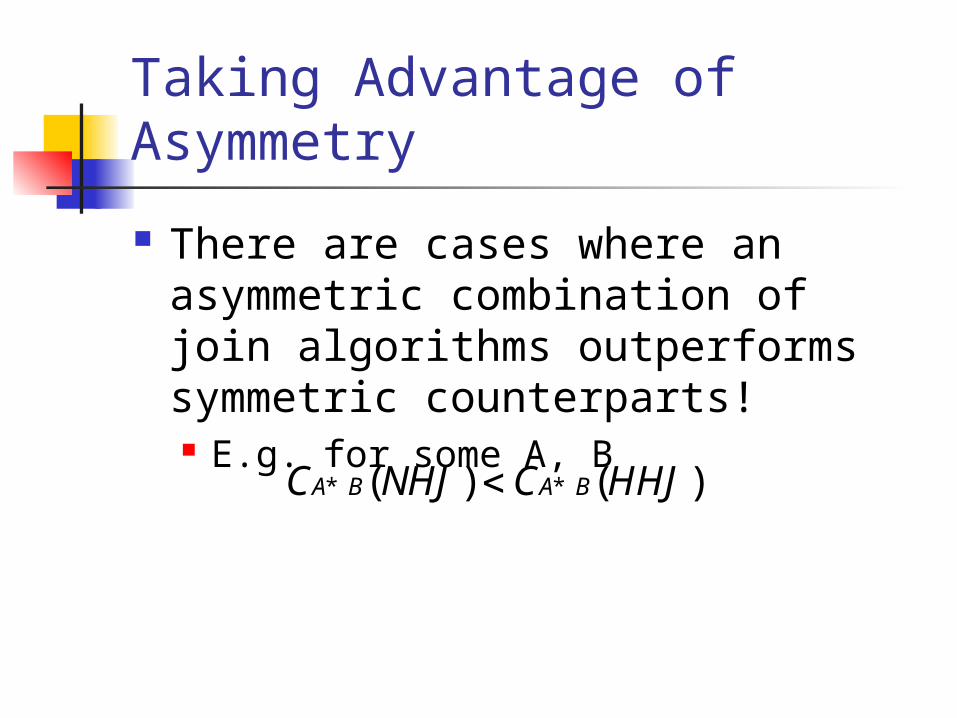
Taking Advantage of Asymmetry

There are cases where an asymmetric combination of join algorithms outperforms symmetric counterparts! E.g. for some A, B

( ) ( )A B A BC NHJ C HHJ* *

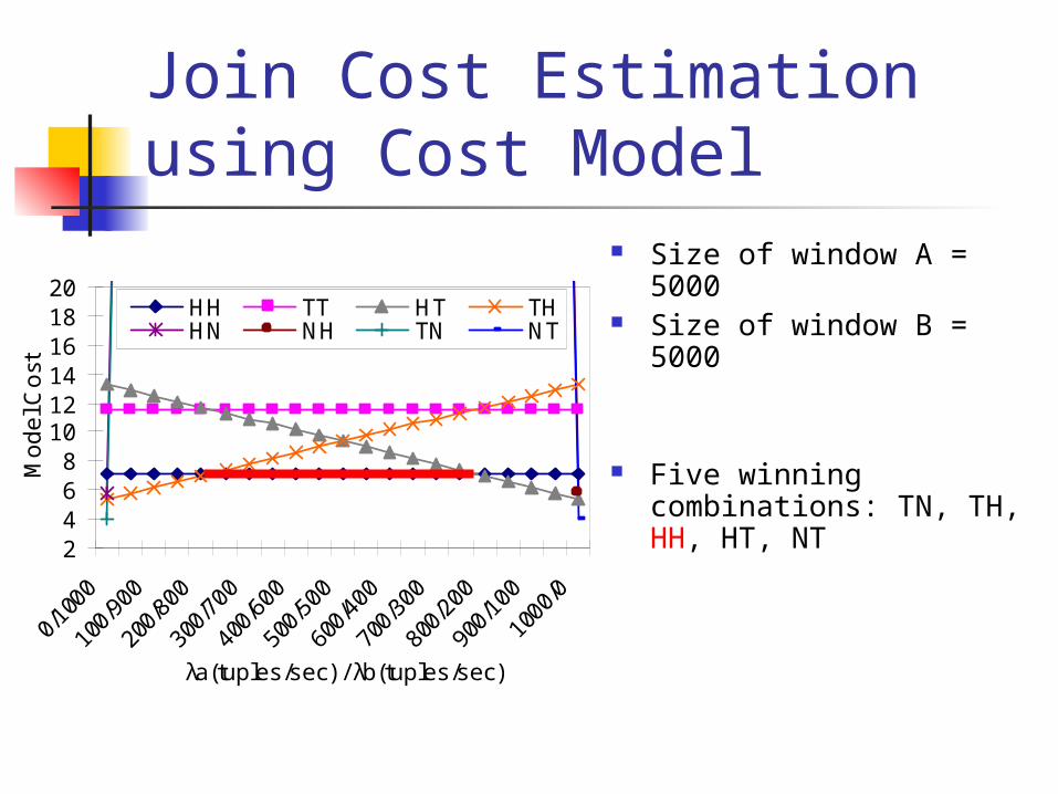
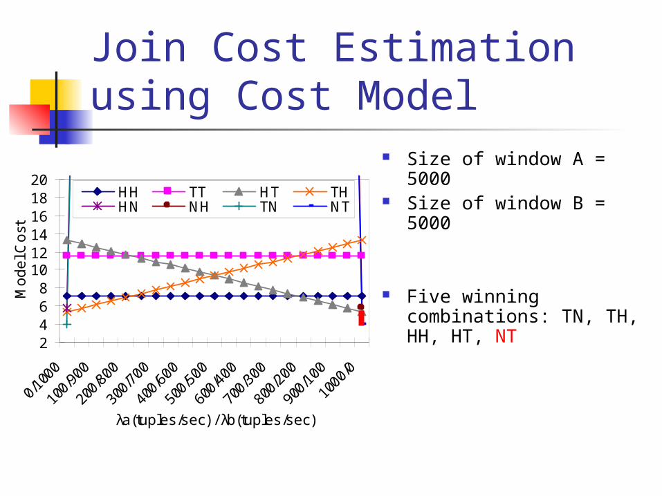
Join Cost Estimation using Cost Model

Size of window A = 5000 Size of window B = 5000

Five winning combinations: TN, TH, HH, HT, NT

2468

101214161820

0/10

00

100/

900

200/

800

300/

700

400/

600

500/

500

600/

400

700/

300

800/

200

900/

100

1000

/0

λa(tuples/sec) / λb(tuples/sec)

Mo

de

l Co

st

HH TT HT THHN NH TN NT

Measured Join Cost (CPU Time)

A=5000, B=5000 Memory utilization: HJ

(h=10) consumed 5% more than TJ (n=100).

Same five winners: TN, TH, HH, HT, NT

Cost model prediction was accurate for both overall shape and crossover points.

500

1500

2500

3500

4500

5500

6500

0/10

00

100/

900

200/

800

300/

700

400/

600

500/

500

600/

400

700/

300

800/

200

900/

100

1000

/0

λa(tuples/sec) / λb(tuples/sec)

CP

U T

ime

(m

illis

)

HH TT HT THHN NH TN NT

What if we increase window A and decrease window B? (e.g. A=7000, B=3000 as opposed to current 5000:5000)

Cross-over Point TN-TH

( ) ( )

( ( ) ( )) ( ( ) ( ))

( ) ( ) 0

13.6

3 55

A B A B

A B A B A B A B

A B A B

a

b

C TNJ C THJ

C TJ C NJ C TJ C HJ

C NJ C HJ

B

* *

( ) ( )

) )

TN-TH only dependent on window size B TN-TH = 0.0094 (B=500), meaning TNJ will

outperform THJ when stream B is more than 106 times faster than stream A.

TN-TH = 0.0555 (B=100), 18 times.

λaTa

λa λb

λbTbA B

Cross-over Point TH-HH

2 2

2 2

( ) ( ) ( ) ( ) 0

58.9 3.9 log 2.6 log

8.1 log 2.7 log 23.7

A B A B A B A B

a

b

C THJ C HHJ C TJ C HJ

AN

NA

NN

* * ( (

TH-HH only dependent on the size of window A If the size of window A increases the crossover

point TH-HH will move toward left, and vice versa.

A=9500, B=500, λa=2, λb=998

Join Performance

0

200

400

600

800

1000

#of Input Tuples Processed

CP

U T

ime

(milli

s)

HHTTHTTHHNTN

A=7000, B=3000, λa=800,λb=200

0200

400600

8001000

12001400

#of Input Tuples Processed

CP

U T

ime

(milli

s) HHTTHTTH

Interesting questions (Cont’d)

How should we allocate computing resources between the two windows to maximize join efficiency?

If memory is the bottleneck, how should we allocate memory between the two windows for the two inputs?

Resource Allocation & Join Performance

Focus on cases where system resources are insufficient to fully support queries and workloads. Input streams are simply too fast to keep

up with. Evaluating expensive join operator and its

service rate is lower than the input rates. System memory cannot hold both

windows.

Resource Allocation & Join Performance (Cont’d) Approximate answers may be acceptable

E.g. query involving aggregate (e.g. average) over join

Question is how to maximize the accuracy of the approximate answers, given the limited resources.

We use insight that larger samples produce better answers

Goal is to maximize the #of join result tuples Care must be taken to ensure that the result

produced is statistically comparable to a random sample of the full join result.

Limited Computing Resources

λa=800, λb=200 A=100, B=200 =0.01, μ=100

( )o a br B A

( ) where , , o a b a b a a b br B A ( )o ar B A A

Window Join Output Rate :w/ Effective Rates =

0

1000

2000

3000

4000

5 10 15 20 25 30 35 40 45 50 55 60Execution T ime (seconds)

Out

put S

ize

(num

ber

of tu

ples

)

Max λaMax λbλ ProportionalWindow ProportionalEqual Distribution

Limited Memory Resources

λa=10, λb=50 M=1000, =0.005

( )o a br B A Window Join Output Rate =

0

5000

10000

15000

20000

5 10 15 20 25 30 35 40 45 50 55 60

Execution T ime (seconds)

Out

put S

ize

(num

ber

of tu

ples

) Max AMax Bλ Proportionalλ InverseEqual Distribution

( ) where (total avaliable memory)o a br B A A B M

( )o b a ar A M

Limited Memory & Computing Resources

μ=10, M=100 =0.01

0100

200300

400500

600

5 10 15 20 25 30 35 40 45 50 55 60

Execution T ime (seconds)

Ou

tpu

t Siz

e (n

um

ber

of tu

ple

s)

Max A / Max λbMax B / Max λaMax A / Max λaMax B / Max λbEqual Distribution

( )

where , , ,

o a b

a b a a b b

r B A

A B M

Best performers are groups that allocate maximum computing resources to one stream and maximum memory to the another.

Summary Introduced unit-time basis cost model and

experimentally validated it.

Extended traditional join framework to include asymmetric combinations of join algorithms.

Investigated resource allocation strategies for improving the accuracy of approximate answers.

Developed powerful optimization framework for sliding window join queries by addressing these issues in a unified manner.

evaluating window joins over unbounded streams

Documents

cost of sliding window

window ascan window

window ainvalidate

join efficiency

window b bb

join algorithms

unbounded streamsmeasuring

search operation id