TRANSPORTATION RESEARCH RECORD 1328 21

Evaluating the Sensitivity of Travel Demand Forecasts to Land Use Input Errors

JIT N. BAJPAI

The sensitivity of the urban transportation planning process (UTPP) to differences (or errors) in socioeconomic input is examined using the Dallas-Fort Worth area as a case study. The sensitivity analysis indicated that the final output of the UTPP, link volumes, is sensitive to errors in the district-level forecasting of population and employment. Planners undertaking corridor-level studies should be most concerned about the reliability and accuracy of district-level socioeconomic forecasts, particularly for districts di­rectly served by the corridor. Because local transportation facil­ities are most sensitive to errors in zone-level inputs, site-specific studies may be severely affected by data errors at the traffic zone level. Greater attention should be paid to suburban areas where the potential for introducing large input errors is high. Because of the potential for large assignment errors, expansion of a district-to-district trip table to a zone-to-zone trip table should be avoided. Travel demand models must be applied using traffic zone-level data, not district-level data.

The Urban Transportation Planning Process (UTPP), com­prising a sequence of models, is commonly used to analyze and predict traffic volumes on a transportation network on the basis of anticipated changes in socioeconomic variables such as population, employment, vehicle availability, income, and household size. To produce an accurate geographic dis­tribution of trip making, these models are usually applied at the traffic zone level using the regional transportation system network- and zone-level socioeconomic inputs. Agencies re­sponsible for the preparation of zone-level data, in general, develop inputs in two steps: first, from region to district and, second, from district to zone (J). Because events that influ­ence the location of economic activities and population are difficult to predict, allocation errors are inevitable though of different magnitude in the two steps of allocation.

Large errors in the forecast of socioeconomic variables are likely to produce highly inaccurate traffic forecasts for deci­sion makers responsible for investment in transportation in­frastructure. For instance, a large disparity between the fore­cast and actual traffic can cause substantial misallocation of public resources due to under- or overdesign of a facility. A recent comparative analysis of 10 urban rail transit projects (2) indicated that overestimates of future population and em­ployment in downtown areas were sufficiently large to con­tribute significantly to overestimation of future ridership on some rail projects built with federal funds. Acknowledging this, it becomes necessary for a transportation planner to

COMSIS Corporation, Suite 1100, 8737 Colesville Road, Silver Spring, Md. 20910. Current affiliation: World Bank, 1818 H Street, N.W., Washington, D.C. 20433.

understand the implications of various types and magnitudes of socioeconomic input errors on the prediction of travel de­mand. This issue is examined by analyzing the sensitivity of travel demand forecasts to land use input errors.

Prior works on the propagation of errors in the travel pre­diction process mostly considered errors caused by the structure of models, input data size, and aggregation procedures. For example, one of the early works on the sensitivity of the four­step travel prediction process to model specification errors and sampling variation in data used was conducted by CONSAD in 1968 (3). Later, efforts were made to analyze errors in prediction with disaggregate choice models. Koppelman ( 4) identified ma­jor sources of errors in prediction, including model error and aggregation error, and suggested ways to improve prediction models.

The sensitivity analysis reported in this paper differs from earlier efforts. The focus of this analysis was on evaluating only the impact of changes in the input of socioeconomic data on the UTPP outputs; other inputs of the process (network data, travel data, and zone structure and the models) were kept the same. The same travel demand model was repeatedly applied to avoid the effect of changes in the structure of the model on traffic forecasts. The Dallas-Fort Worth area travel demand model was selected for the sensitivity tests. Five sce­narios representing various types and magnitudes of errors in district and subdistrict (zone) allocations were tested.

APPROACH

Selected Travel Demand Model

The Dallas-Fort Worth area travel demand model was se­lected for the sensitivity tests. The selection considered the sophistication of and familiarity with travel demand models as well as staff skill levels in their maintenance and operation. However, the foremost factor was the willingness of the North Central Texas Council of Governments (NCTCOG) to assist in the analysis. NCTCOG currently uses the DRAM/EMP AL (5) models to allocate regional land use forecasts for the nine­county Dallas-Fort Worth area to 170 forecast districts. The district forecasts are subsequently allocated to almost 5,691 traffic survey zones (TSZs). Travel demand simulation models produce assignments for transit and highway networks using the TSZ-level socioeconomic variable inputs (households; median income; and employment by basic, retail, and service categories) and mode-specific network attributes (6). The model

22

generates interzonal trip tables for four income categories (low, low-middle, high-middle, and high) and four trip pur­poses (home-based work, home-based nonwork, non-home based, and other). The four-step modeling process (trip gen­eration, trip distribution, mode choice, and network assign­ment) includes three sophisticated multinomial logit type mode choice models for each of the three trip purposes (excluding "other" purpose).

The trip distribution model uses a standard gravity for­mulation technique and a second-order Bessel curve as the travel decay function for each of the seven trip purposes (home­based work for three income groups, home-based nonwork, non-home based, and other). Minimum time of travel be­tween zones is used as the impedance measure in the distribu­tion models.

For roadway traffic assignment a capacity-restrained as­signment model with an incremental loading procedure is ap­plied. A generalized cost function of time, distance, and toll is used in building the minimum paths between zones. The model uses the upper and lower bounds of the total number of trips (defined as 20,000 and 100,000 trips) and the critical volume-to-capacity ratio (set at 0.8) as three parameters for controlling link updating. As the network becomes congested, the trips assigned between each successive link updating de­crease from the upper bound toward the lower bound. Two separate volume-delay equations are used for high- and low­capacity facilities. Further distinction is made between the daily and peak-hour assignment models. As the volume-to­capacity ratio exceeds 0. 7, the delay rises exponentially to the maximum allowable delay.

Because all sensitivity tests were performed for the base year, the mode shares (transit and highway) represented the observed shares in the base year. In other words, mode-split models were not used while running the entire model chain. The primary intent was to examine the effect of allocation errors on highway trip assignments only. The daily assignment procedure was applied, and estimates of daily link volumes were converted to hourly units using factors of 0.10 and 0.12 for high- and low-capacity facilities, respectively.

Scenarios of Land Use Input Errors

Traffic zone-level inputs are usually prepared in two steps: first, from region to district and second, from district to zone. Most agencies use two separate methods for each of the two steps of forecasting. The difference between the input fore­casts and reality, referred to here as errors in allocation/fore­casting, can occur at either step, though the errors are of different magnitude and nature. "Nature of error" means the pattern of error distribution in the geographical space. Errors can be concentrated in a few locations, reflecting a geograph­ical bias, or distributed in a random fashion. The contem­porary phenomenon of rapid suburban growth, for example, can easily produce underprediction of employment in the sub­urbs and overprediction in the central city. This can occur if the forecasting/allocation method used for district forecasts fails to anticipate, for example, the magnitude and trend of suburbanization in high-technology service jobs. Similarly, one or more biased parameters in an analytical method can produce allocation errors of almost random nature.

TRANSPORTATION RESEARCH RECORD 1328

To illustrate the effect of errors (or changes) in socioeco­nomic input data on the UTPP outputs, five scenarios, repre­senting various types and magnitudes of errors in district and subdistrict allocations, were formulated. In addition, a sep­arate test scenario was developed to examine the impact of assigning a zone-to-zone trip interchange table that was pro­duced by disaggregating a district-to-district trip table instead of using a trip table generated directly by the application of travel demand models at the zone level. The intent behind this scenario was to examine whether the practice among certain agencies of expanding a trip table to develop a smaller spatial unit level trip interchange table is accurate. In practice, a district-level trip table, an output of either a trip distribution model or a land use simulation model such as DRAM/ EMPAL (5), POLIS (7), or PLUM (8), is often disaggregated into a zonal trip using a proportioning method.

Although many test scenarios could be evaluated, the fol­lowing six tests addressed the issues of land use allocation mentioned previously within the available resources.

• Errors in district level allocation were evaluated by Test A (introduce ± 20 percent random errors into land use fore­casts at the district level) and Test B (introduce ± 40 percent random errors into land use forecasts at the district level) .

• Errors in subdistrict level allocation were evaluated by Test C (introduce geographical bias into land use allocation at the district level), Test D (introduce ± 40 percent random errors into land use forecasts at the zone level), and Test E (distribute district forecasts uniformly among zones compos­ing a district).

• Trip table disaggregation was evaluated by Test F (dis­aggregate district-level trip table to zone level).

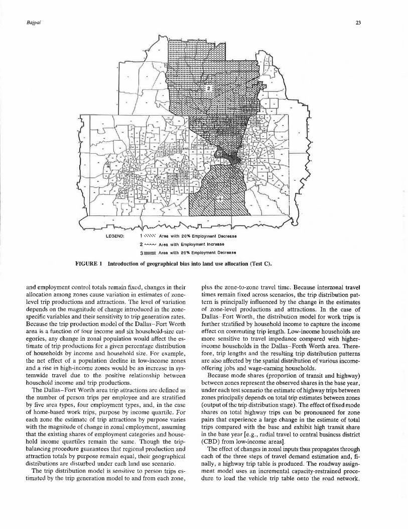
For Tests A, B, and D, the distribution of error was created by randomly selecting one-third of districts or zones for pos­itive, one-third for negative, and one-third for no errors. The overall magnitude of positive error was kept equal to negative error and distributed in proportion to population and em­ployment. For Test C, employment for the downtown district and the districts in the southwestern sector of Dallas was reduced by 20 percent, and the same magnitude of employ­ment increase was allocated among districts located in the northwestern sector (Figure 1) in the same proportion as ex­isting employment. For developing uniform distribution under Test E, traffic zone-level data were prepared by dividing the district forecasts by the number of zones (i.e., PIN, where P and N represent the population and the number of zones in a district, respectively) . For Test F, an 800 x 800 trip inter­change table was first collapsed into a 147 x 147 table and then expanded back to an 800 x 800 table using zonal shares of households and employment in each district. The number of households and total employment were used as the pro­portioning factors for trip productions and attractions, respectively.

Sensitivity of Travel Models to Zone-Level Inputs

Changes introduced in zonal socioeconomic inputs affect all four steps of travel forecasting: trip generation, distribution, mode choice, and assignment. Even though the population

..

Bajpai 23

LEGEND: 1 '''''' Area with 20% Employment DecreaH

2 ~ Area with Employment Increase

3»'~ Area with 20% Employment Decrease

FIGURE 1 Introduction of geographical bias into land use allocation (Test C).

and employment control totals remain fixed, changes in their allocation among zones cause variation in estimates of zone­level trip productions and attractions. The level of variation depends on the magnitude of change introduced in the zone­specific variables and their sensitivity to trip generation rates. Because the trip production model of the Dallas-Fort Worth area is a function of four income and six household-size cat­egories, any change in zonal population would affect the es­timate of trip productions for a given percentage distribution of households by income and household size. For example, the net effect of a population decline in low-income zones and a rise in high-income zones would be an increase in sys­temwide travel due to the positive relationship between household income and trip productions.

The Dallas-Fort Worth area trip attractions are defined as the number of person trips per employee and are stratified by five area types, four employment types, and, in the case of home-based work trips, purpose by income quartile. For each zone the estimate of trip attractions by purpose varies with the magnitude of change in zonal employment, assuming that the existing shares of employment categories and house­hold income quartiles remain the same. Though the trip­balancing procedure guarantees that regional production and attraction totals by purpose remain equal, their geographical distributions are disturbed under each land use scenario.

The trip distribution model is sensitive to person trips es­timated by the trip generation model to and from each zone,

plus the zone-to-zone travel time. Because interzonal travel times remain fixed across scenarios, the trip distribution pat­tern is principally influenced by the change in the estimates of zone-level productions and attractions. In the case of Dallas-Fort Worth, the distribution model for work trips is further stratified by household income to capture the income effect on commuting trip length. Low-income households are more sensitive to travel impedance compared with higher­income households in the Dallas-Forth Worth area. There­fore, trip lengths and the resulting trip distribution patterns are also affected by the spatial distribution of various income­offering jobs and wage-earning households.

Because mode shares (proportion of transit and highway) between zones represent the observed shares in the base year, under each test scenario the estimate of highway trips between zones principally depends on total trip estimates between zones (output of the trip distribution stage). The effect of fixed mode shares on total highway trips can be pronounced for zone pairs that experience a large change in the estimate of total trips compared with the base and exhibit high transit share in the base year [e.g., radial travel to central business district (CBD) from low-income areas].

The effect of changes in zonal inputs thus propagates through each of the three steps of travel demand estimation and, fi­nally, a highway trip table is produced. The roadway assign­ment model uses an incremental capacity-restrained proce­dure to load the vehicle trip table onto the road network.

24

Because the assignment process is sensitive to congestion, a significant change in the orientation of vehicle trips can trigger traffic diversion. The output of this step is road link volumes, the final outcome of the four-step process. Hence, a com­parison of the base year and individual test scenario specific link volumes illustrates the magnitude of overall traffic impact caused by a particular scenario. In other words, changes in link volumes manifest the accumulated effect of the zone­level input changes on link-level travel.

Traffic Impact Measures

For each test scenario, the effect of introducing a certain type and magnitude of socioeconomic input error on the final out­put of UTPP is measured at both the systemwide level and the micro level. The output measures of individual test runs and the run without any error (base run) are compared to illustrate the magnitude of the effect.

At the system level, root mean square error (RMSE), av­erage trip length, and total number of trips are considered as aggregate output measures of UTPP. The final UTPP output is traffic volumes assigned on a particular transportation sys­tem network or a group of links. To check the accuracy of UTPP, however, the assigned link volumes are generally com­pared with the ground counts (or ridership counts in the case of transit). RMSE is usually calculated to indicate the overall goodness of fit between traffic counts and model assigned traffic volumes. It is measured in the following manner:

RMSE 2: (count - assigned volume )2

(N - 1)

where N is the number of traffic count stations. Because of the large number of trip interchanges in an area,

average trip length is a commonly used summary measure of trip distribution patterns. Similarly, the total number of trips is a simple measure of trip generation model output.

To examine the micro-level effects of each sensitivity test, lane error, a measure reflecting the difference between the test case assigned link volume and the base case (without error) link volume, is calculated for individual links. Lane error for a link is defined as

test case link volume - base link volume Lane error = ---------------­

link capacity • number of lanes

Link capacity is expressed in terms of vehicles per hour per lane. It varies with the type of facility (freeways, major ar-

TRANSPORTATION RESEARCH RECORD 1328

terial, minor arterial, and collector) and area type (downtown, suburb, etc.). Lane error is a measure of discrepancy in traffic volume easily understood by transportation planners and highway engineers. A road planning rule of thumb suggests that a forecast error not exceeding one half-lane (positive or negative) is tolerable without a high probability of under- or overdesigning a facility. In other words, it reflects the mag­nitude of public resource misallocation that may occur be­cause of the error in traffic forecasts.

FINDINGS OF SENSITIVITY TESTS

Errors in Distict Level Land Use Forecasts

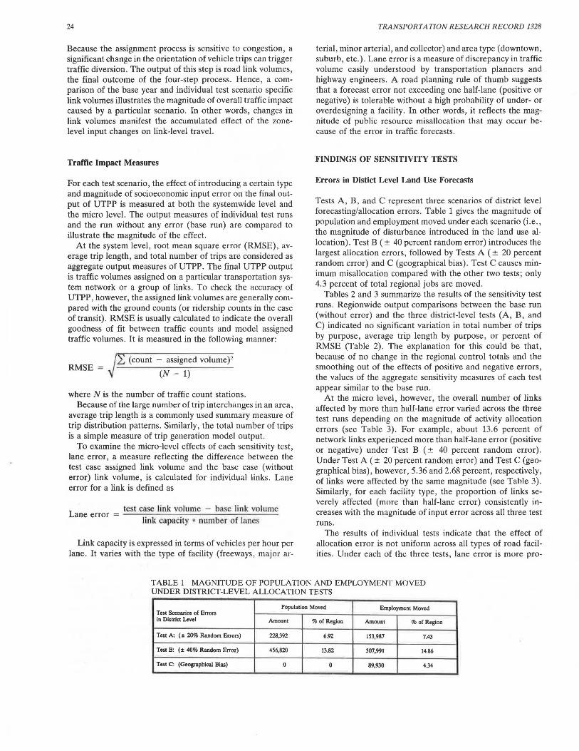
Tests A, B , and C represent three scenarios of district level forecasting/allocation errors. Table 1 gives the magnitude of population and employment moved under each scenario (i.e., the magnitude of disturbance introduced in the land use al­location). Test B ( ± 40 percent random error) introduces the largest allocation errors, followed by Tests A ( ± 20 percent random error) and C (geographical bias). Test C causes min­imum misallocation compared with the other two tests; only 4.3 percent of total regional jobs are moved.

Tables 2 and 3 summarize the results of the sensitivity test runs. Regionwide output comparisons between the base run (without error) and the three district-level tests (A, B, and C) indicated no significant variation in total number of trips by purpose, average trip length by purpose, or percent of RMSE (Table 2). The explanation for this could be that, because of no change in the regional control totals and the smoothing out of the effects of positive and negative errors, the values of the aggregate sensitivity measures of each test appear similar to the base run.

At the micro level, however, the overall number of links affected by more than half-lane error varied across the three test runs depending on the magnitude of activity allocation errors (see Table 3). For example, about 13.6 percent of network links experienced more than half-lane error (positive or negative) under Test B ( ± 40 percent random error). Under Test A ( ± 20 percent random error) and Test C (geo­graphical bias), however, 5.36 and 2.68 percent, respectively, of links were affected by the same magnitude (see Table 3). Similarly, for each facility type, the proportion of links se­verely affected (more than half-lane error) consistently in­creases with the magnitude of input error across all three test runs.

The results of individual tests indicate that the effect of allocation error is not uniform across all types of road facil­ities. Under each of the three tests, lane error is more pro-

TABLE 1 MAGNITUDE OF POPULATION AND EMPLOYMENT MOVED UNDER DISTRICT-LEVEL ALLOCATION TESTS

Test Scenarios of Errors Population Moved Employment Moved

in District Level Amount % of Region Amount % of Region

Test A: ( :t 20% Random Errors) 228,392 6.92 153,987 7.43

Test B: (:t 40% Random Error) 456,820 13.82 307,991 14.86

Test C: (Geographical Bias) 0 0 89,930 4.34

Bajpai 25

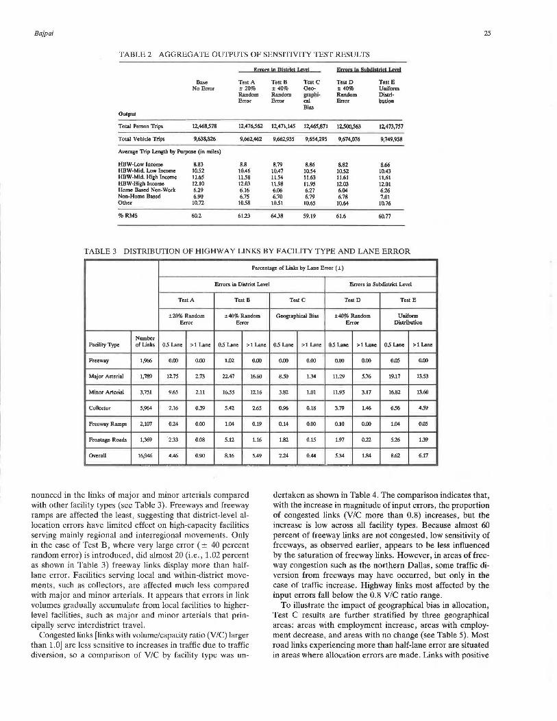
TABLE2 AGGREGATE OUTPUTS OF SENSITIVITY TEST RESULTS

Ema ID Dll ld'I Leri Emra In Sybdlnrlct 1.«ycl

Base Test A TestB TestC TestD Test E No Error ± 20% ± 40% Geo- ± 40% Uniform

Random Random snphl· Random Distrl· Error Error cal Error bution

Bias Output

Total Person Trips 12,468,578 12,476,562 12,471,145 12,465,871 12,500,563 12,473,757

Total Vehicle Trips 9,638,826 9,662,462 9,662,935 9,654,295 9,674,076 9,749,958

Average Trip Length by Purpose (in miles)

HBW-Low Income 8.83 8.8 8.79 8.86 8.82 8.66 HBW-Mid. Low Income 10.52 10.46 10.47 10.54 10.52 10.43 HBW-Mid. High Income 11.65 11.58 11.54 11.63 11.61 11.61 HBW-High Income 12.10 12.03 11.98 11.95 12.03 12.01 Home Based Non-Work 6.29 6.16 6.06 6.27 6.04 6.26 Non-Home Based 6.90 6.75 6.70 6.79 6.78 7.01 Other 10.72 10.58 10.51 10.65 10.64 10.76

%RMS 60.2 61.23 64.38 59.19 61.6 60.77

TABLE 3 DISTRIBUTION OF HIGHWAY LINKS BY FACILITY TYPE AND LANE ERROR

Percentage of Links by Lane Error ( ±)

Errors in District Level

Test A Test B

±20% Random ±40% Random Error Error

Number Facility Type of Links 0.5 Lane >1 Lane 05 Lane >1 Lane

Freeway 1,966 0.00 0.00 1.02

Major Arterial 1,789 12.75 2.73 22.47

Minor Arterial 3,751 9.65 2.11 1655

Collector 5,964 2.16 0.39 5.42

Freeway Ramps 2,107 0.24 0.00 1.04

Frontage Roads 1,369 2.33 0.08 5.12

Overall 16,946 4.46 0.90 8.16

nounced in the links of major and minor arterials compared with other facility types (see Table 3). Freeways and freeway ramps are affected the least, suggesting that district-level al­location errors have limited effect on high-capacity facilities serving mainly regional and interregional movements. Only in the case of Test B, where very large error ( ± 40 percent random error) is introduced, did almost 20 (i.e., 1.02 percent as shown in Table 3) freeway links display more than half­lane error. Facilities serving local and within-district move­ments, such as collectors, are affected much less compared with major and minor arterials. It appears that errors in link volumes gradually accumulate from local facilities to higher­level facilities, such as major and minor arterials that prin­cipally serve interdistrict travel.

Congested links [links with volume/capacity ratio (V/C) larger than 1.0] are less sensitive to increases in traffic due to traffic diversion, so a comparison of V/C by facility type was un-

0.00

16.60

12.16

2.65

0.19

1.16

5.49

Errors in Subdistrict Level

TestC Test D Test E

Geographical Bias ±40% Random Uniform Error Distribution

05 Lane >1 Lane 0.5 Lane >1 Lane 0.5 Lane >1 Lane

0.00 0.00 0.00 0.00 0.05 0.00

8.50 1.34 11.29 5.76 19.17 13.53

3.82 1.01 11.95 3.17 16.82 13.60

0.96 0.18 3.79 1.46 6.56 4.59

0.14 0.00 0.10 0.00 1.04 0.05

1.82 0.15 1.97 0.22 5.26 1.39

2.24 0.44 5.34 1.84 8.62 6.17

dertaken as shown in Table 4. The comparison indicates that, with the increase in magnitude of input errors, the proportion of congested links (V/C more than 0.8) increases, but the increase is low across all facility types. Because almost 60 percent of freeway links are not congested, low sensitivity of freeways, as observed earlier, appears to be less influenced by the saturation of freeway links. However, in areas of free­way congestion such as the northern Dallas, some traffic di­version from freeways may have occurred, but only in the case of traffic increase. Highway links most affected by the input errors fall below the 0.8 V/C ratio range.

To illustrate the impact of geographical bias in allocation, Test C results are further stratified by three geographical areas: areas with employment increase, areas with employ­ment decrease, and areas with no change (see Table 5). Most road links experiencing more than half-lane error are situated in areas where allocation errors are made. Links with positive

26 TRANSPORTA TJON RESEARCH RECORD 1328

TABLE 4 DISTRIBUTION OF HIGHWAY LINKS BY FACILITY TYPE AND V/C RATIO

Distribution of Uaka (in %) % Change in I.he Distribulioo of Links Compared lo Base

Errors in District uvel

Test A Tc.ID nasc Case +I- 20 rcrccnt ltanJom Error + /- 40 Pcrccnl Random Error

Pacilily Type < 0.8 0.8 - 1.0 > 1.00 < 0.8 O.H-1.0 > 1.00 < 0.8 0.8 - 1.0 > 1.00

Freeway 59.92 10.89 29.20 0.10 -0.31 0.20 -1.93 0.15 1.78

Major Arterial 47.18 11.85 4.97 -2.24 0.17 -0.11 -2.40 -0.11 2.52

Minor Arterial 75.23 8.93 15.84 0.05 0,56 -0.61 -0.64 J_(J.1 ·0.40

Colleclor 89.40 3.24 7.36 -0.15 0.03 0.12 0.07 -0.17 0.10

Freeway Ramps 79.69 6.03 14.29 -0.33 0.09 0.24 -1.00 0.90 0,()9

Fronlage Roads 81.67 4.60 13.73 -0.37 0.15 0.22 -1.17 0.07 1.10

Overall 76.55 6.75 16.69 -0.11 0.14 -0.04 -0.81 0,30 0.5!

TABLE 5 LANE ERRORS BY GEOGRAPHICAL AREAS UNDER TEST C (GEOGRAPHICAL BIAS)

Facility Number Areas wilh No Change Type o£Linlcs +0.5 Lane ->0.5 Lane

Freeways 1966 0 0

Major Arterial 1789 7 13 % of Links 0.39 0.73

Minor Arterial 3751 6 1 % of Links .16 0.03

Collector 5964 2 11 % of Links 0.03 0.18

Freeway Ramps 2107 0 0 % of Links 0.00 0.00

Frontage Roads 1369 2 6 % of Links 0.15 0.44

Total 16946 17 31

% of Links 100.00 0,10 0.18

(overestimation of traffic) and negative lane error are con­centrated in areas with employment increase and decrease, respectively. For instance, out of 455 road links with greater than half-lane error, 228 links serving areas of employment increase indicated positive error, and 166 links situated in areas where employment is reduced indicated negative error. As observed earlier, the most affected links are concentrated in the categories of major and minor arterials. Overall, al­though the percentage of links severely affected appears low (2.68 percent with more than half-lane error) due to a small magnitude of geographical bias in district inputs (Test C), the affected number of links is high enough (176 major and 181 minor arterial links) to cause misallocation of public resources.

Errors in the Disaggregation of District-Level Inputs to Zone Level

Tests D ( ± 40 percent random error) and E (uniform distribu­tion) are extreme cases of subdistrict allocation errors. Test

Areas w /Employmenl Increase Areas w /Employmenl Deaease +0.5 Lane ->0.5 Lane +0.5 Lane ->0.5 Lane

0 0 0 0

89 2 4 61 4.97 0.11 0.22 3.41

86 2 0 86 2.1.9 0.05 0.00 2-29

41 4 0 10 0.69 0.07 0.00 0.17

0 0 0 3 0.00 0.00 0.00 0.14

12 1 0 6 0.88 0.07 0.00 0.44

228 9 4 166

l.3S 0.05 .02 0.98

E presents a case where zone-level forecasts are prepared with no consideration given to zonal capacity, zoning policy, or other major factors influencing the attractiveness of a zone for development (e.g., transportation accessibility, availabil­ity of public services , existing development , etc.). Test D, however, reflects a case of large random error in allocation. To illustrate the level of disturbance caused under each of the two scenarios, R2 values for zonal population and em­ployment are estimated by comparing the inputs for the base (no error) and individual test runs separately (Table 6). In this case, the R2 value reflects the strength of association between the base case inputs and particular test run inputs. A value of 1 represents a perfect match between the two sets, and 0 means no match. The higher values of R2 (0.917 for population and 0.915 for employment) observed under Test D (±40 percent random error) clearly indicate that this test does not cause as large a deviation from the base case allo­cation as Test E (uniform distribution). Actually, uniform distribution under Test E causes an extremely large error in zonal inputs.

Bajpai

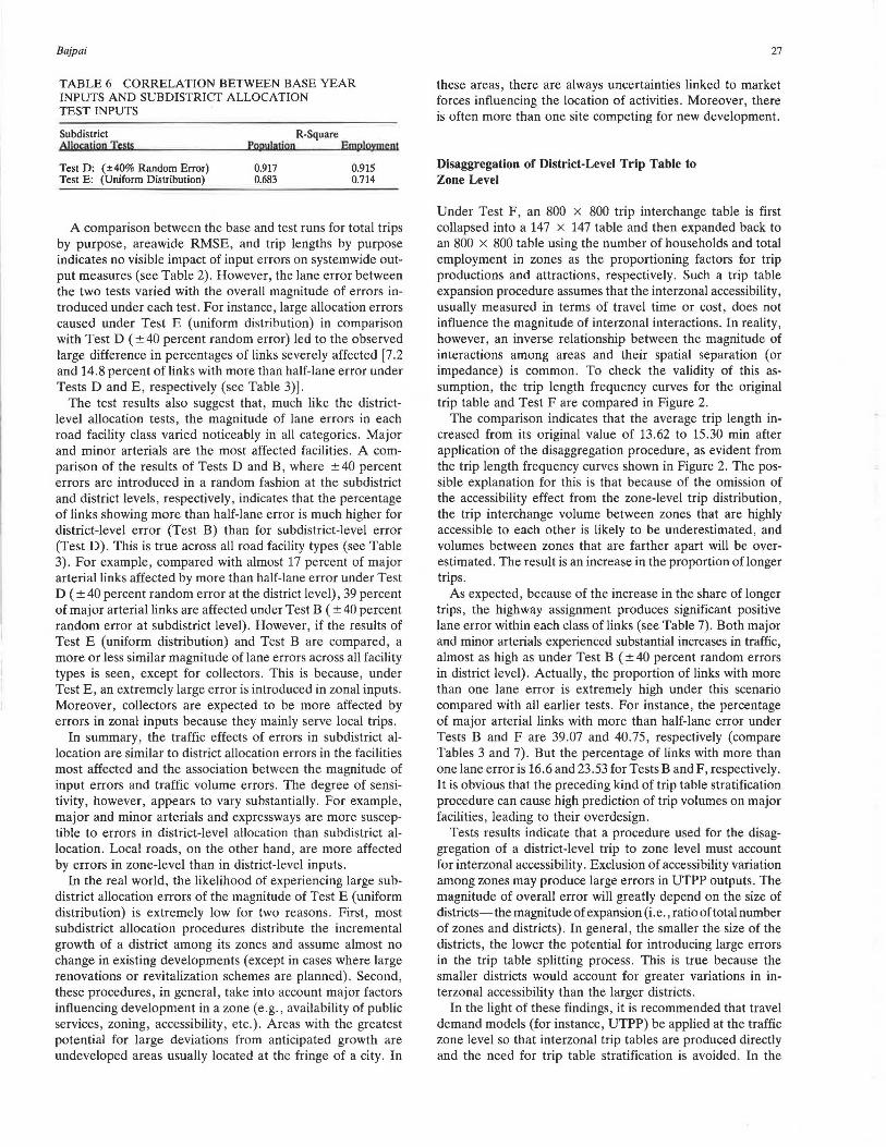
TABLE 6 CORRELATION BETWEEN BASE YEAR INPUTS AND SUBDISTRICT ALLOCATION TEST INPUTS

Subdistrict Al!oca1jon Tests

Test D: (±40% Random Error) Test E: (Uniform Distribution)

R-Square Population Employmem

0.917 0.683

0.915 0.714

A comparison between the base and test runs for total trips by purpose, areawide RMSE, and trip lengths by purpose indicates no visible impact of input errors on systemwide out­put measures (see Table 2). However, the lane error between the two tests varied with the overall magnitude of errors in­troduced under each test. For instance, large allocation errors caused under Test E (uniform distribution) in comparison with Test D ( ± 40 percent random error) led to the observed large difference in percentages of links severely affected [7.2 and 14.8 percent of links with more than half-lane error under Tests D and E , respectively (see Table 3)].

The test results also suggest that, much like the district­level allocation tests, the magnitude of lane errors in each road facility class varied noticeably in all categories. Major and minor arterials are the most affected facilities. A com­parison of the results of Tests D and B, where ± 40 percent errors are introduced in a random fashion at the subdistrict and district levels, respectively, indicates that the percentage of links showing more than half-lane error is much higher for district-level error (Test B) than for subdistrict-level error (Test D). This is true across all road facility types (see Table 3). For example , compared with almost 17 percent of major arterial links affected by more than half-lane error under Test D ( ± 40 percent random error at the district level), 39 percent of major arterial links are affected under Test B ( ± 40 percent random error at subdistrict level). However, if the results of Test E (uniform distribution) and Test B are compared, a more or less similar magnitude of lane errors across all facility types is seen , except for collectors. This is because, under Test E, an extremely large error is introduced in zonal inputs. Moreover, collectors are expected to be more affected by errors in zonal inputs because they mainly serve local trips.

In summary, the traffic effects of errors in subdistrict al­location are similar to district allocation errors in the facilities most affected and the association between the magnitude of input errors and traffic volume errors. The degree of sensi­tivity, however, appears to vary substantially. For example, major and minor arterials and expressways are more suscep­tible to errors in district-level allocation than subdistrict al­location. Local roads, on the other hand, are more affected by errors in zone-level than in district-level inputs.

In the real world, the likelihood of experiencing large sub­district allocation errors of the magnitude of Test E (uniform distribution) is extremely low for two reasons. First, most subdistrict allocation procedures distribute the incremental growth of a district among its zones and assume almost no change in existing developments (except in cases where large renovations or revitalization schemes are planned). Second, these procedures, in general, take into account major factors influencing development in a zone (e.g., availability of public services, zoning, accessibility, etc .). Areas with the greatest potential for large deviations from anticipated growth are undeveloped areas usually located at the fringe of a city. In

27

these areas, there are always uncertainties linked to market forces influencing the location of activities. Moreover, there is often more than one site competing for new development.

Disaggregation of District-Level Trip Table to Zone Level

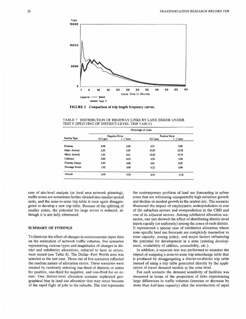
Under Test F, an 800 x 800 trip interchange table is first collapsed into a 147 x 147 table and then expanded back to an 800 x 800 table using the number of households and total employment in zones as the proportioning factors for trip productions and attractions, respectively. Such a trip table expansion procedure assumes that the interzonal accessibility , usually measured in terms of travel time or cost , does not influence the magnitude of interzonal interactions. In reality, however, an inverse relationship between the magnitude of interactions among areas and their spatial separation (or impedance) is common . To check the validity of this as­sumption, the trip length frequency curves for the original trip table and Test F are compared in Figure 2.

The comparison indicates that the average trip length in­creased from its original value of 13.62 to 15.30 min after application of the disaggregation procedure, as evident from the trip length frequency curves shown in Figure 2. The pos­sible explanation for this is that because of the omission of the accessibility effect from the zone-level trip distribution, the trip interchange volume between zones that are highly accessible to each other is likely to be underestimated, and volumes between zones that are farther apart will be over­estimated. The result is an increase in the proportion of longer trips.

As expected, because of the increase in the share of longer trips, the highway assignment produces significant positive lane error within each class of links (see Table 7). Both major and minor arterials experienced substantial increases in traffic, almost as high as under Test B ( ± 40 percent random errors in district level) . Actually, the proportion of links with more than one lane error is extremely high under this scenario compared with all earlier tests. For instance, the percentage of major arterial links with more than half-lane error under Tests B and F are 39.07 and 40.75, respectively (compare Tables 3 and 7) . But the percentage of links with more than one lane error is 16.6 and 23.53 for Tests Band F, respectively. It is obvious that the preceding kind of trip table stratification procedure can cause high prediction of trip volumes on major facilities, leading to their overdesign.

Tests results indicate that a procedure used for the disag­gregation of a district-level trip to zone level must account for interzonal accessibility. Exclusion of accessibility variation among zones may produce large errors in UTPP outputs. The magnitude of overall error will greatly depend on the size of districts-the magnitude of expansion (i.e., ratio of total number of zones and districts). In general , the smaller the size of the districts, the lower the potential for introducing large errors in the trip table splitting process. This is true because the smaller districts would account for greater variations in in­terzonal accessibility than the larger districts.

In the light of these findings , it is recommended that travel demand models (for instance, UTPP) be applied at the traffic zone level so that interzonal trip tables are produced directly and the need for trip table stratification is avoided. In the

28 TRANSPORTATION RESEARCH RECORD 1328

Trips 15000 .---~~~~~~~~~~~~~~~~~~~~~~~~~

10000

5000

5 10 15 . 20 25 30 35 40 45 50 55

Travel Time In Minutes Legend:········· Base

-Test F

FIGURE 2 Comparison of trip length frequency curves.

TABLE 7 DISTRIBUTION OF HIGHWAY LINKS BY LANE ERROR UNDER TEST F (SPLITIING OF DISTRICT-LEVEL TRIP TABLE)

Negative Error Facility Type 0.5 Lane > 1 Lane

Freeway 0.00

Major Arterial 2.35

Minor Arterial 1.52

Collector 0.89

Freeway Ramps 0.05

Frontage Roads 1.02

Overall 0.99

case of site-level analysis (or local area network planning), traffic zones are sometimes further divided into smaller spatial units, and the zone-to-zone trip table is once again disaggre­gated to develop a new trip table. Because of the splitting of smaller zones, the potential for large errors is reduced, al­though it is not fully eliminated.

SUMMARY OF FINDINGS

To illustrate the effect of changes in socioeconomic input data on the estimation of network traffic volumes, five scenarios representing various types and magnitudes of changes in dis­trict and subdistrict allocations, referred to here as errors, were tested (see Table 8). The Dallas-Fort Worth area was selected as the test case. Three out of five scenarios reflected the random nature of allocation errors. These scenarios were created by randomly selecting one-third of districts or zones for positive, one-third for negative, and one-third for no er­rors. One district-level allocation scenario replicated geo­graphical bias in land use allocation that may occur because of the rapid flight of jobs to the suburbs. The test represents

0.00

0.95

0.41

0.32

0.00

0.00

0.29

Percentage of Llnks

Positive Error 0.5 Lane > 1 Lane

0.51 0.00

14.87 22.58

13.01 13.74

4.59 3.30

0.81 0.05

6.22 6.90

6.44 6.76

the contemporary problem of land use forecasting in urban areas that are witnessing unexpectedly high suburban growth and decline or modest growth in the central city. The scenario illustrated the impact of employment underprediction in one of the suburban sectors and overprediction in the CBD and one of its adjacent sectors. Among subdistrict allocation sce­narios, one test showed the effect of distributing district-level inputs equally (or uniformly) among the zones of each district. It represented a special case of subdistrict allocation where zone-specific land use forecasts are completely insensitive to zone capacity, zoning policy, and major factors influencing the potential for development in a zone (existing develop­ment, availability of utilities, accessibility, etc.).

In addition, a separate test was performed to examine the impact of assigning a zone-to-zone trip interchange table that is produced by disaggregating a district-to-district trip table instead of using a trip table generated directly by the appli­cation of travel demand models at the zone level.

For each scenario the demand sensitivity of facilities was measured in terms of the proportion of links experiencing large differences in traffic volumes (increase or decrease by more than half-lane capacity) after the introduction of input

Bajpai 29

TABLE 8 FINDINGS OF SENSITIVITY TESTS

Tnllic lmpKt mi Pacilitica

-------- ---- ---------------------------- ----- ---Collect on

>--·------------ -------·---.--... ------------------·-Prom Region to District Random Small Not significant Moderate ww

Random Large ww High '-<>w /Moderate

Geographical Small Not Significant Moderate but '-<>w Bias conccntlated in areu

with input errors

------- ------------ ·-Prom District to Zones Random Large Not Significant Moderate ww /Moderate

Uniform Large WW High Moderate

------ ·----------·-- ----------- ·---------------------------------Splitting of Trip Table ww High Moderate/High

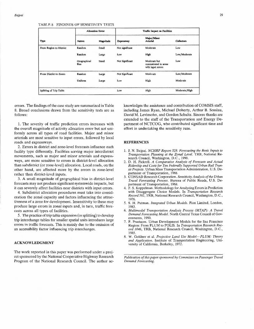
errors. The findings of the case study are summarized in Table 8. Broad conclusions drawn from the sensitivity tests are as follows:

1. The severity of traffic prediction errors increases with the overall magnitude of activity allocation error but not uni­formly across all types of road facilities. Major and minor arterials are most sensitive to input errors , followed by local roads and expressways.

2. Errors in district and zone-level forecasts influence each facility type differently. Facilities serving major interdistrict movements, such as major and minor arterials and express­ways, are more sensitive to errors in district-level allocation than subdistrict (or zone-level) allocation. Local roads, on the other hand, are affected more by the errors in zone-level rather than district-level inputs.

3. A small magnitude of geographical bias in district-level forecasts may not produce significant systemwide impacts, but it can severely affect facilities near districts with input errors .

4. Subdistrict allocation procedures must take into consid­eration the zonal capacity and factors influencing the attrac­tiveness of a zone for development. Insensitivity to these may produce large errors in zonal inputs and, in turn, traffic fore­casts across all types of facilities .

5. The practice of trip table expansion (or splitting) to develop trip interchange tables for smaller spatial units introduces large errors in traffic forecasts. This is mainly due to the omission of an accessibility factor influencing trip interchanges.

ACKNOWLEDGMENT

The work reported in this paper was performed under a proj­ect sponsored by the National Cooperative Highway Research Program of the National Research Council. The author ac-

knowledges the assistance and contribution of COMSIS staff, including James Ryan, Michael Doherty, Arthur B. Sosslau, David M. Levinsohn, and Gordon Schultz. Sincere thanks are extended to the staff of the Transportation and Energy De­partment of NCTCOG, who contributed significant time and effort in undertaking the sensitivity runs .

REFERENCES

1. J. N. Bajpai. NCHRP Report 328: Forecasting the Basic Inputs to Transportation Planning at the Zonal Level. TRB, National Re­search Council, Washington, D.C., 1990.

2. D . H. Pickrell . A Comparative Analysis of Forecasts and Actual Ridership and Costs for Ten Federally Supported Urban Rail Tran­sit Projects . Urban Mass Transportation Administration, U .S. De­partment of Transportation, 1988.

3. CONSAD Research Corporation. Sensitivity Analysis of the Urban Travel Forecasting Process . Bureau of Public Roads, U.S . De­partment of Transportation, 1968.

4. F. S. Koppelman. Methodology for Analyzing Errors in Prediction with Disaggregate Choice Models . In Transportation Research Record 592, TRB, National Research Council, Washington, D.C., 1976.

5. S. H . Putman. Integrated Urban Models . Pion Limited, London, 1983.

6. Multimodal Transportation Analysis Process (MTAP) : A Travel Demand Forecasting Model . North Central Texas Council of Gov­ernments, 1990.

7. P. Prastacos. Urban Development Models for the San Francisco Region : From PLUM to POLIS. In Transportation Research Rec­ord 1046, TRB, National Research Council, Washington, D.C., 1985.

8. W. Goldner et al. Projective Land Use Model-PLUM: Theory and Application. Institute of Transportation Engineering, Uni­versity of California, Berkeley, 1972.

Publication of this paper sponsored by Committee on Passenger Travel Demand Forecasting.