evaluating the quality of intelligent controllers for 3

Evaluating the Quality of Intelligent Controllers

for 3-DOF Delta Robot Control

Le Minh Thanh, Luong Hoai Thuong, Pham Thanh Tung Vinh Long University of Technical Education, Vietnam

Email: [email protected], {thuonglh, tungpt}@vlute.edu.vn

Cong-Thanh Pham Viet Nam Aviation Academy, Vietnam

Email: [email protected]

Chi-Ngon Nguyen *

Can Tho University, Vietnam


Abstract—Delta robots have been successfully researched

and manufactured in many countries. In this paper, the

authors will research and compare many different

controllers to control the delta robot so that it works

stability when changing the working speed and load. The

regression fuzzy neural network along with PID controller

(RFNNC-PID) is used to observe the output error

parameters of the robot through the identifier to update and

adjust the optimal input parameters to control the robot,

contributing error reduction of the closed-loop control

system. The advantage of this controller is that it does not

care about the robot's mathematical model and the RFNNC-

PID controller has been successfully simulated by the

authors in MATLAB/Simulink through the robot's

trajectory control. The proposed controller will be

compared to the single neuron PID controller and the

traditional PID controller in MATLAB/Simulink. The

simulation results show that the proposed controller is

better than the single neuron PID controller and the

traditional one with obtaining response time about 3.8 ± 0.1

(s) and without steady-state error.

Index Terms—Delta robot, single neural PID, recurrent

fuzzy neural network, Identifier, trajectory tracking.

Symbol Unit Meaning

1 2 3, , rad/s Angles the upper leg of the robot

1 2 3, , rad/s Passive angles determine the position

of the connection points

R m Radius of the fixed plate

r m Radius of the moving plate

L1 m Length of upper arm

L2 m Length of upper arm

m1 kg Mass of upper arm

m2 kg Mass of lower arm

mP kg Mass of the moving plate

O m The center of the fixed plate

P m The center of the moving plate

Ai m The connection point of the upper legs

Manuscript received November 16, 2020; revised March 25, 2021. (*) Corresponding author: Chi-Ngon Nguyen, Can Tho University,


with the fixed plate

Bi m The connection point of the upper legs

with the lower legs

Di m The connection point of the lower legs

with the moving plate

Abbreviation

PID Proportional Integral Derivative

DOF Degrees of freedom

RFNNC Recurrent Fuzzy Neural Network Controller

RFNNI Recurrent Fuzzy Neural Network Identifier

I. INTRODUCTION

Parallel robot is a kind of closed multi-loop

mechanism and is widely used in industrial fields thanks

to its high rigidity, high precision and outstanding weight

and load ratio [1], [2]. Parallel Delta robot was adopted in

many complex fields, for example: microelectronics [3],

[4], medicine [5], [6], logistics intelligence [7], [8], and

3D printing [9], [10]. In those complex applications, the

high-precision control of Delta parallel robots has

become an important issue for researchers. One of these

studies is the PD and LQR controllers presented by Joao

Fabian [11]. In this paper, Joao Fabian used embedded NI

my RIO hardware programmed in LabView software to

compare the two PD controllers and LQR robot trajectory

controllers. The nonlinear PID shown by the HAN [12] is

used to replace increment scheduling with a nonlinear

gain function by introducing a continuous dynamic

nonlinear function to achieve better noise cancel-lation

and better tracking, this is achieved by the synthesis of a

function consists of a linear function close to zero error

and a nonlinear function far from zero error. The third

technique is using a PD controller with intelligent

compensation that is used to solve the trap trajectory

tracking for a parallel delta robot with three degrees of

freedom presented by Ahmed Chemori [13]. Ahmed

Chemori tested a PID controller that performs the

542

International Journal of Mechanical Engineering and Robotics Research Vol. 10, No. 10, October 2021

© 2021 Int. J. Mech. Eng. Rob. Resdoi: 10.18178/ijmerr.10.10.542-552

reference trajectory tracking of a real delta robot with

extremely high acceleration up to 100 G as shown in [14]

Recently, several controllers are proposed to control

the parallel robot. In [15], R. Anoop and K. Achu

designed and verified the performance of the adaptive

PID driving a parallel Delta controller. In that work, the

controller was able to track the desired trajectory without

any discouragement. In [16], Zhang et al. studied the

problem of dynamic control for redundantly actuated

planer 2-DOF parallel manipulator. The work proposed

an augmented PD controller based on the forward

dynamic compensation control technique, which showed

better performance when compared to conventional PD

controls. In [17], Hussein Saied et al. proposed different

model-based (augmented PD and adaptive feedforward

with PD) controllers and non-model-based (PD, PID, and

nonlinear PD) controllers for a 4-DOF parallel VELOCE

robot. Experimental results indicated that the nonlinear

control method can achieve a superior performance [18].

Su et al. developed a nonlinear proportional integral

derivative algorithm in link space to achieve high

precision tracking control for a general 6-DOF parallel

manipulator.

The PID controllers have been successfully developed

for 6-DOF robots. However, when changing robot’s

parameters such as load, input coupling and friction, the

PID controllers are difficult to archive control criteria by

their fixed parameters. So that, the neural networks and

fuzzy logic are applied to improve controlling of Delta

robot [19]. The RFNN controllers and identifiers have

been developed and applied for nonlinear systems [20-24].

During control process, the RFNN identifier can estimate

the object's sensitivity, called Jacobian information. That

information is used for online training the RFNN

controller. Therefore, by using RFNN, the control

technique is flexible to adjust its parameters online

adapting to the control conditions.

In this paper, the group of authors makes two main

contributions. Firstly, the team set up the motion equation

of the parallel delta robot (including the equations of the

forward kinetics, the reverse kinetics, the delta robot

dynamics) and successfully simulated the motion

equations of the delta robots on MATLAB / Simulink.

Secondly, the optimal RFNNC-PID is built and

successfully simulated to control the trajectory of the

delta robot on an ellipse curve and eight curve in

MATLAB / Simulink and make sure this trajectory is

always stable with the changes of control conditions.

This paper is organized consists of five sections. An

introduction is Section I; Section II presents the construct

mathematical models of the 3-DOF delta robot; trajectory

tracking control of the 3-DOF delta robot is presented in

Section III; compare the simulation results of the three

controllers are presented in Section IV and Section V is

the conclusion.

II. CONSTRUCT MATHEMATICAL MODELS OF THE 3-

DOF DELTA ROBOT

A. Kinetic Models of the 3-DOF Delta Robot

The dynamics of the delta robot are shown in Fig. 1

which consists of two equal triangles (fixed plate and

movable plate).

Figure 1. Rotation angle and position of delta robot.

The common angles are 1 ,

2 ,3 , the point P is the

end point location with coordinates (xP, yP, zP). To

calculate the inverse kinetics of delta robot, we have to

know in advance the position of the end point P(xP, yP,

zP), from there we go back to the opposite angle 1 ,

2 ,

3 . Conversely, to find the forward dynamics of delta

robot, we have to know the angles in advance, and then

we find the endpoint position P (xP, yP, zP)

1) Reverse kinetics of delta robot

The reverse kinetics in this paper require to obtain the

desired angular position of the actuator given the desired

endpoint of the effect in Cartesian space. This is a

geometrical method, so weight and moment of inertia are

not considered during modeling.

The physical geometry and the real robotic delta model

are shown in Fig. 2

The geometrical shape of the delta

robot

Realistic delta robot model

made by authors

Figure 2. The physical geometry and the real robotic delta model.

In Fig. 2: R is the radius of the fixed plate, r is the

radius of the moving plate, f represents the length of the

equilateral triangle of the upper platform, e is the length

of the equilateral side of the lower-moving disc, L1 the

upper leg length, L2 length of the lower leg,

, ,P P PP x y z is the center of the low-moving disc,

1 1 11 , ,D D DD x y z is the midpoint of the equilateral triangle

of the lower-moving disc, and D1 is the connection point

of the lower leg to the motion plate, 0 (0,0,0) is the center

of the top fixed plate, the point A1 is the midpoint of the

equilateral triangle of the top fixed plate, and A1 is the

connection point of the upper leg to the fixed plate. The

P (xP, yP, zP)

543


© 2021 Int. J. Mech. Eng. Rob. Res

angles 1 ,

2 ,

3 , are the driving angles of the three

mechanical arms, point B1 is the intersection point

between the upper leg and the lower leg of the delta robot.

Due to the structure of the delta robot, A1B1 can only

rotate around the YZ axis to form a circle with the

center point A1 and radius L1. In contrast to A1B1, point D1

is seen as a composite joint, meaning that D1B1 can rotate

freely depending on point D1 forming a sphere with

center D1 and radius L2.

The intersections between a sphere and a circle are

shown in Fig. 3

Figure 3. The geometric intersection between a sphere and a circle.

In the Fig. 3 points D’1 is the projection of point D1 on

the YZ plane. The point B1 can be found at the

intersection point of two circles C1 and C2 with the

centers are A1 and D'1 respectively, and the radius L1 and

D'1B1 respectively, if we find B1 then we can Calculates

the rotation angle of the robot and B1 is found the

following circle formulas

Equation of the circle C1:

1 1 1 1 1 1

2 22

1B A B A B Ax y y y z z L (1)

With points 1 0, ,0

2 3

fA

and 1 11 0, ,B BB y z are

found from Fig. 3, then deduced:

1 1

2

2 2

12 3

B B

fy z L

Equation of the circle C2:

1 1 1 1

2 2 22 2 '

' ' 1 1 2 1 1'B D B Dy y z z D B L D D (2)

With points '

1 x , y ,z2 3

P P P

eD

and '

1 1 PD D x ,

then deduced:

1 1

22

2 2

22 3

B P B P P

ey y z z L x

We need to find the point 1 11 0, ,B BB y z through

equations (1) and (2), and if we know in advance the

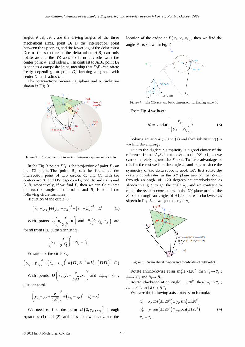
location of the endpoint , ,P P PP x y z , then we find the

angle 1 as shown in Fig. 4

Figure 4. The YZ-axis and basic dimensions for finding angle θ1.

From Fig. 4 we have:

1

11

1 arctan ?B

BA

z

y y

(3)

Solving equations (1) and (2) and then substituting (3)

we find the angle1 .

Due to the algebraic simplicity is a good choice of the

reference frame: A1B1 joint moves in the YZ-axis, so we

can completely ignore the X axis. To take advantage of

this for the rest we find the angle 2

and 3

, and since the

symmetry of the delta robot is used, let's first rotate the

system coordinates in the XY plane around the Z-axis

through an angle of -120 degrees counterclockwise as

shown in Fig. 5 to get the angle 2

, and we continue to

rotate the system coordinates in the XY plane around the

Z-axis through an angle of +120 degrees clockwise as

shown in Fig. 5 so we get the angle 3

Figure 5. Symmetrical rotation and coordinates of delta robot.

Rotate anticlockwise at an angle -1200 then

1 →

2 ;

A1→ A’1 and B1→ B’1

Rotate clockwise at an angle +1200 then

1 →

3 ;

A1→ A’’1 and B1→ B’’1

We have the following axis conversion formula:

0 0

0 0

cos 120 sin 120

sin 120 cos 120

i

P P P

i

P P P

i

P P

x x y

y y x

z z

(4)

544



With i = 2, 3

From the axis conversion formula we deduce the

formula of angle 2

as follows:

2 0 0

2 0 0

2

cos 120 sin 120

sin 120 cos 120

P P P

P P P

P P

x x y

y y x

z z

(5)

With i = 2, Similar to finding angle 1 , we substitute (5)

into (1) and (2) and solve the solution for solution, then

we replace the solution we just found in (6) we find angle

2 :

1

1 1

'

2

' '

arctanB

A B

z

y y

(6)

We have the following formula for changing the axis

of angle 3

:

3 0 0

3 0 0

3

cos 120 sin 120

sin 120 cos 120

P P P

P P P

P P

x x y

y y x

z z

(7)

With i = 3

We substitute (7) into (1) and (2) and solve the

solution for solution, then we replace the solution we just

found in (8) we find angle 3

1

1 1

''

3

'' ''

arctanB

A B

z

y y

(8)

Constructing the inverse kinetic block of the delta

robot in Simulink by giving the endpoint position

, ,P P PP x y z , we will find the angles 1 ,

2 ,

3 of the

delta robot through the formulas (3), (6) and (8).

2) The forward kinetics of delta robot

A forward motion is used to reach the end position

using the upper leg angles. The representative geometry

of a robot leg is shown in Fig. 6 [25]

Figure 6. Geometrical parameters of a robotic delta leg.

From Fig. 7, we have a global variable like this:

i m , eff iD n

2i iB D L , 1i iB L

where point i ∈ {1, 2, 3} refers to pins on 1, 2, 3 and Σ is

the global reference system, Σi is the reference system for

the above pins, Σeff is the reference system for the end

points, Bi is the connection point between the upper and

lower legs, Di is the connection point between the lower

leg and the fixed plate,i are the angles of the upper legs

and i

are the angles separating each upper leg and the

XY plane.

Lower leg length can be calculated using the following

vector relation:

i i i iD B D B (9)

Equation (9) can be written in terms of the geometrical

length of the robot and the position Di with due the

correlation to reference Σ, as follows:

1

1

cos cos

0 sin

sin 0

i

i i

i

Di n i

i i n i D

i D

xL

D B R y

L z

(10)

Inside, Δn = m - n and i

R is the rotation matrix

between the Σi and Σ of the reference system

The i

R contained in the equation (10) is bound by the

following length:

2 2

2i iD B L , with i =1,2,3 (11)

Equation (11) is rewritten as follows:

2 2 2

2

2i i i i i iD B D B D Bx x y y z z L (12)

With i = 1, 2, 3

Substituting equation (12) for (10) gives the following

formula:

1

1

1

cos cos

cos sin

sin

i

i

i

B n i i

B n i i

B i

x L

y L

z L

(13)

From equation (13), if we give the angles i

and i

then we will find the position 1 1 11 , ,B B BB x y z of delta

robot. After finding the point 1 1 11 , ,B B BB x y z from

equation (13), then we replace equation (12) solve

equation finding for point 1 1 11 , ,D D DD x y z , we deduce

the end point location , ,P P PP x y z

Constructing the forward kinetic block of the delta

robot in Simulink by giving the corners 1 ,

2 ,

3 of the

delta robot, we will find the endpoint position

, ,P P PP x y z of the delta robot through the formulas (12)

and (13).

545



B. Dynamic Model of a 3-DOF Delta Robot

The best model for a 3-DOF delta robot is a system of

rigid bodies connected by joints. The parallelogram

mechanisms that connect the driving links to the mobile

platform are modeled as homogeneous rods with

universal and spherical joints at two ends. By using this

model, the robot is seen as a multibody system with seven

bodies: three legs each leg having two links and the

mobile platform. The calculating models are shown in Fig.

7 [21], [27].

Figure 7. Calculating models of a 3-DOF delta robot [21].

Putting i , i = 1, 2, 3 be the driving angles of the

actuated links;1

, i = 1, 2, 3 be the passive angles that

determine the position of the connecting rods; and

, ,T

P P PP x y z be the position of the center of mass of

the mobile platform. Hence, the position of robot is

determined by the generalized coordinates:

𝑞 = [𝜃1 𝜃2 𝜃3 𝑥𝑃 𝑦𝑃 𝑧𝑃]

Set the differential equation of motion of the 3-DOF

delta robot

The motion equation is established by using the

Lagrange formula:

𝑑

𝑑𝑡(𝜕𝑇

𝜕�̇�𝑘) −

𝜕𝑇

𝜕𝑞𝑘= 𝑄𝑘 −∑ 𝜆𝑖

𝜕𝑓𝑖

𝜕𝑞𝑘(𝑘 = 1,2, … . ,𝑚)𝑟

𝑖=1 (14)

where qk is the extrapolation coordinates of the robot, fi is

the linking equations, Qk is the extrapolation force, i is

the Lagrange factor. With this model, the vector of

extrapolation coordinates 6R and the number of

associated equations is three, so m = 6, r = 3. We divide

the forces acting on the robot into potential forces and

forces without potential energy, the extrapolation force

Qk is calculated as follow

np

k k

k

Q Qq

(15)

In it np

kQ are extrapolation forces corresponding to

forces that are not possible. Virtual power of

extrapolation is not so:

𝛿𝐴 = 𝜏1𝛿𝜃1 + 𝜏2𝛿𝜃2 + 𝜏3𝛿𝜃3 (16)

So we have: 1 1 2 2 3 3, ,np np npQ Q Q , cases 0np

kQ

with k = 4, 5, 6. Substituting kinetic expressions,

potentials and equations into equation (14), we get the

motion equation of the robot as the system. The

differential equation-algebra is as follows:

(𝐼𝐼𝑦 +𝑚𝑏𝑙12)�̈�1 = 𝑔𝑙1 (

1

2𝑚1 +𝑚𝑏) 𝑐𝑜𝑠 𝜃1 + 𝜏1

−2𝜆1𝑙1 (𝑠𝑖𝑛 𝜃1 (𝑅 − 𝑟) − 𝑐𝑜𝑠 𝛼1 𝑠𝑖𝑛 𝜃1 𝑥𝑝−𝑠𝑖𝑛 𝛼1 𝑠𝑖𝑛 𝜃1 𝑦𝑝 − 𝑐𝑜𝑠 𝜃1 𝑧𝑝

) (17)

(𝐼𝐼𝑦 +𝑚𝑏𝑙12)�̈�2 = 𝑔𝑙1 (

1



) (18)

(𝐼𝐼𝑦 +𝑚𝑏𝑙12)�̈�3 = 𝑔𝑙1 (

1



) (19)

(𝑚𝑝 + 3𝑚𝑏)�̈�𝑝 =

−2𝜆1(𝑐𝑜𝑠 𝛼1 (𝑅 − 𝑟) + 𝑙1 𝑐𝑜𝑠 𝛼1 𝑐𝑜𝑠 𝜃1 − 𝑥𝑝)

−2𝜆2(𝑐𝑜𝑠 𝛼2 (𝑅 − 𝑟) + 𝑙1 𝑐𝑜𝑠 𝛼2 𝑐𝑜𝑠 𝜃2 − 𝑥𝑝) (20)

−2𝜆3(𝑐𝑜𝑠 𝛼3 (𝑅 − 𝑟) + 𝑙1 𝑐𝑜𝑠 𝛼3 𝑐𝑜𝑠 𝜃3 − 𝑥𝑝)

(𝑚𝑝 + 3𝑚𝑏)�̈�𝑝 =

−2𝜆1(𝑠𝑖𝑛 𝛼1 (𝑅 − 𝑟) + 𝑙1 𝑠𝑖𝑛 𝛼1 𝑐𝑜𝑠 𝜃1 − 𝑦𝑝)

−2𝜆2(𝑠𝑖𝑛 𝛼2 (𝑅 − 𝑟) + 𝑙1 𝑠𝑖𝑛 𝛼2 𝑐𝑜𝑠 𝜃2 − 𝑦𝑝) (21)

−2𝜆3(𝑠𝑖𝑛 𝛼3 (𝑅 − 𝑟) + 𝑙1 𝑠𝑖𝑛 𝛼3 𝑐𝑜𝑠 𝜃3 − 𝑦𝑝)

(𝑚𝑝 + 3𝑚𝑏)�̈�𝑝 =

−(3𝑚𝑏 +𝑚𝑝)𝑔 + 2𝜆1(𝑧𝑝 + 𝑙1 𝑠𝑖𝑛 𝜃1) (22)

+2𝜆2(𝑧𝑝 + 𝑙1 𝑠𝑖𝑛 𝜃2) + 2𝜆3(𝑧𝑝 + 𝑙1 𝑠𝑖𝑛 𝜃3)

22

1 1 1 1 1

2

1 1 1 1

2

1 1

cos coscos

sin

sin 0p

p

p

l R r l x

R r l y

zl

22

2 2 1 2 2

2

2 1 2 2

2

1 2

cos cos

sin cos (24)

cos

sin

sin 0p

p

p

l R r l x

R r l y

zl

22

3 3 1 3 3

2

3 1 3 3

2

1 3

cos cos

sin cos (25)

cos

sin

sin 0p

p

p

l R r l x

R r l y

zl

From the motion equations of the parallel robot (17) to

(25), according to the proposal [21], [26], [27] we will

construct the model of the 3-DOF Delta robot in

MATLAB/Simulink.

546



sin cos (23)

III. TRAJECTORY TRACKING CONTROL OF THE 3-DOF

DELTA ROBOT

A. Delta Robot Control Using a Single Neuron PID

The control system for a robot arm is presented in Fig.

8

Figure 8. Controller structure [21].

The reference signal yref is the rotation angle of the

upper three arms of the robot is sent to three adders

giving three error signals e1, e2, e3 to three PID controllers

one neuron, the output of three the controller was inserted

into Tau1, Tau2, Tau3 of the 3-DOF Delta Robot. At the

same time, three RFNN identifiers will observe three

outputs of three single-neuron PID controllers and three

output signals y (theta1, theta2, theta3) of delta robot,

each RFNN identifier will train the parameter Jacobian

returned three single-neuron PID controllers to

continuously update the KP, KD, and KI parameters of the

three controllers to control the delta robot following

the reference signal yref presented by the authors in [21]

B. The 3-DOF Delta Robot Control Using RFNNC-PID

1) The 3-DOF delta robot RFNN identifier

The identifier is shown in Fig. 9 that consists of 4

layers, with a 2-node input layer, a 10-node fuzzy layer, a

25-node fuzzy rule, and a 1-node output layer [28]-[32].

Figure 9. Delta robot model in MATLAB/Simulink.

Layer 1 (Input layer): This layer takes the input

variables and passes the input values to the next layer.

Feedback lines are added in this layer to embed time

relations into the network. The output of layer 1 is

represented as (26):

1 1 1 1 , 1,2k

i i i iO k x k O k i (26)

With 1

i is the connection weight at the current time k.

The input of the corresponding RFNN is the current

control signal and the past output of the response:

1 1

1 2, 1x k u k x k y k (27)

Figure 10. Structure of four-layer RFNN.

Layer 2 (Fuzzy layer): This layer consists of (2x5)

nodes, each node representing a related function of the

Gaussian form with mean value mij and standard

deviation σij, and defined as (28).

21

2

2exp , 1,2; 1,2,...,5

i ij

ij

j

O k mO k i j

i

(28)

At each node on the fuzzy layer, there are 2 parameters

that are automatically adjusted during the online training

of the RFNN identifier, that is mij and σij.

Layer 3 (Rule layer): This layer provides fuzzy

inferences. Each node corresponds to a fuzzy rule. The

link before each node represents the prerequisites of the

respective rule. The qth the fuzzy law can be described:

3 2 , 1,2,...,5; 1,2,...,5q iq iii

O k O k i q (29)

Layer 4 (Output layer): This layer includes 1 linear

neuron with the defined output as follows:

4 4 3 , 1; 1,2,...,25i ij jj

O k w O k i j (30)

where 4

ijw is the connecting weights from 3rd layer to 4th

layer. The output of this layer is also the output of the

RFNN:

𝑂14(𝑘) = 𝑦𝑚(𝑘) = 𝑓[𝑥1(𝑘), 𝑥2(𝑘)] = 𝑓[𝑢(𝑘), 𝑦(𝑘 − 1)] (31)

The performance RFNN identifier training is based on

a cost function in (32) [20]:

22 4

1

1 1

2 2I m IE k y k y k y k O k (32)

The RFNN's weights are adjusted according to (33) [20]:

1I I I

I

I I

I

W k W k W k

E kW k

W

(33)

where, I is the learning rate, WI=[I, mI, σI, wI]T

is the

weight vector of RFNN updated during training the

RFNN. And subscript I presents the RFNN identifier,

called RFNNI.

547



Given eI(k)=y(k)-ym(k) is the error between plant’s

output and RFNN’s output, then the gradient EI(.) with

respect to WI is determined as (34):

4

1I m I

I I

I I I

E k y k O ke k e k

W W W

(34)

The weight of each RFNNI network layer is updated as

follows [21], [32]:

4 4 31wI

ij iI Iij I I Iw k w k e k O (35)

1

4 3

2

1

2

Iij Iij

Iij IijmII I Iik Ik

kIij

m k m k

O k me k w O

(36)

3

21

4 3

1

2

Iij Iij

Iij IijII I Iik Ik

kIij

k k

O k me k w O

(37)

1 1

1 1

4 3

1

2 1

2

Ii Ii

Iij Iij IijI

I I Iik Ikk

Iij

k k

O k m O ke k w O

(38)

In addition, to estimate the output of the model ym(k),

the RFNNI must also estimate Jacobian information

( )( )

y ku k

, determined as follows [21], [31], [32]:

13

4

2 2

2 Iij IijIq

Iijq s

IqsIij

O k mOy kw

u k O

(39)

2) Building controller of RFNNC-PID

In this part, for controlling a robot arm, a RFNN

controller (RFNNC) is combined with a traditional PID

controller with its structure is shown in Fig. 11 [21]-[23].

Figure 11 Control system based on RFNNs.

In Fig. 11, the RFNNI is used to identify the model of

the robot, based on y(k-1) and u(k). That makes the

RFNN model is simple and decreases number of neurons.

Through training, the RFNNI estimates the output

trajectories of the delta robot by (30).

Training performance criterion is defined as (40) [20]:

2

C rfnnc

24

C1rfnnc

1E k = u k -u k

2

1u k -O k

2

(40)

where u(k) is the sth

input of the plant,rfnnc

u (k) is the sth

output of RFNNC. After the initialization process, a

gradient-descent-based back-propagation algorithm was

employed to adjust the controller parameters (40):

1C C C

C

C C

C

W k W k W k

E kW k

W

(41)

In which, c is the learning rate, WC=[C, mC, σC, wC]

T

is the weight vector of the RFNNC updated during

training. Subscript C presents the RFNNC.

Given eC(k)=urfnn(k)-u(k), the gradient EC(.) with

respect to WC is defined as (42):

4

1rfnncC

C C

C C C

u kE k O ke k e k

W W W

(42)

The weight of each RFNNC network layer is updated

as follows [21], [30]:

4

4

4

4 3

1

( )

Cw

Cij C

Cij

ijC

wCij iC C C Cpid

E kw k

ww k

w k u k e k O

(43)

1

4 3

2

1

2

Cm

Cij C

Cij

ijC

Cij CijmCCij C C C Cik k

kCij

E km k

mm k

O k mm k e k w O

(44)

21

4 3

3

1

2

C

ij C

Cij

Cij

Cij CijC

Cij C C Cik Ckk

ijC

E kC kk

O k mk e k w O

(45)

1

1

1 1

1 1

4 3

2

1

2 1

C

Ci C

Ci

Ci Ci

Cij Cij CijC

C Cik Ckk

Cij

E kkk k

O k m O ke k w O

(46)

IV. COMPARE THE SIMULATION RESULTS OF THE

THREE CONTROLLERS

A. Simulation Parameters of Three Controllers

The specifications of the real robot that the authors

have built are shown in Table I.

548



TABLE I. DELTA ROBOT MECHANICAL SPECIFICATIONS

Symbol Value Unit

α1 0 rad/s

α2 2π/3 rad/s α3 4π/3 rad/s

R 138.9 mm

r 25 mm f 481.07 mm

e 43.3 mm

L1 250 mm L2 544 mm

m1 0.258 kg

m2=2mb 0.088 kg mp 0.044 kg

The parameters of the Single Neural PID Algorithms,

and Recurrent Fuzzy Neural Network Controller, and

Recurrent Fuzzy Neural Network Identifier are randomly

initialized.

B. Simulation Results

The MATLAB/Simulink control system for a 3-DOF

delta robot with the desired trajectory as an ellipse curve

(47).

x = 0.19sin( t)+0.3

y = 0.12cos( t)+0.2

z = -0.8

d

d

d

(47)

Figure 12. The 3-DOF Delta Robot controller in MATLAB/Simulink.

Figure 13. The angles of theta 1.



Figure 16. Errors of responses.

549



Fig. 13, Fig. 14, Fig. 15 and Fig. 16 comparisons

angles theta of three traditional PID, Single-Neuron PID

controller and RFNN-PID controller.

Figure 17. Trajectory tracking of traditional PID and Single Neuron PID and RFNN-PID controller.

Figure 18. Responses when changing load from 4.71 Kg to 7.05 Kg.

The response of the traditional PID, Single neuron PID

and the RFNN-PID controllers are presented in Fig. 13 –

Fig. 18 including load changed. Simulation results show

that the RFNN-PID controller is better than Single neuron

PID controller, with the setting time is about 3. 8±0. 1

seconds, and the steady-state error is eliminated.

The MATLAB/Simulink control system for a 3-DOF

delta robot with the desired trajectory as a Fig. 8 is shown

(48).

x = 0.15sin(2 t)+0.3

y = 0.15sin(2 t)*cos(2 t)+0. 2

z = -0.7

d

d

d

(48)

Figure 19. Trajectory tracking of the Fig. 8.

And the control criteria of PID controller, Single

Neuron PID and RFNNC-PID controller are presented in

Table II. The results show that the proposed controller

must be better than the Single Neuron PID controller and

traditional PID controller.

TABLE II. SYSTEM CONTROL QUALITY STANDARDS

Respons

e

PID Single Neuron PID RFNN-PID

Rise

time (s)

Overshoot

(%)

Settling

time (s)

Rise

time (s)

Overshoot

(%)

Settling

time (s)

Rise

time (s)

Overshoot

(%)

Settling

time (s)

Theta 1 3.134 1.873 5.6±0.1 3.119 1.799 4.2±0.1 2.942 0.299 3.9±0.1

Theta 2 2.838 1.882 6.9±0.1 2.889 1.992 3.6±0.1 3.346 1.953 3.8±0.1

Theta 3 2.698 1.859 4.2±0.1 2.705 1.973 3.9±0.1 2.447 0.409 3.6±0.1

V. CONCLUSION

In this paper, the RFNN-PID controller is proposed to

control the 3-DOF delta robot. This controller guarantees

the real trajectory converges the reference trajectory with

finite time. The simulation results show that the proposed

controller is better than the single neuron PID controller

and the traditional PID controller. The proposed RFNNC-

PID algorithm is stable while changing the control

conditions such as the speed and load of the delta robot

increasing. In further work, the proposed controller will

be experimenting with the real robot model.

CONFLICT OF INTEREST

The authors declare no conflict of interest.

AUTHOR CONTRIBUTIONS

Mr. Le Minh Thanh, first author, is a PhD student

under supervising of Assoc. Prof. Dr. Chi-Ngon Nguyen

(last and corresponding author), who has prepared the

manuscript. Mr. Luong Hoai Thuong and Mr. Pham

Thanh Tung, 2nd

and 3rd

authors have contributed on

model simulation. Dr. Cong-Thanh Pham, 4th

author, has

contributed on writing correction. Assoc. Prof. Dr. Chi-

Ngon Nguyen is chief of research group, who has

supervised for this study and finalized this paper.

REFERENCES

[1] G. Gao, M. Ye, and M. Zhang, "Synchronous robust sliding mode control of a parallel robot for automobile electro-coating

conveying," IEEE Access, vol. 7, pp. 85838-85847, 2019.

550



[2] S. Qian, B. Zi, D. Wang, and Y. Li, “Development of modular cable-drivenn parallel robotic systems,” IEEE Access, vol. 7, pp.

5541–5553, 2019.

[3] J. E. Correa, J. Toombs, N. Toombs, and P. M. Ferreira, “Laminated micromachine: Design and fabrication of a flexure-

based Delta Robot,” J. Manuf. Processes, vol. 24, pp. 370–375,

Oct. 2016. [4] X. J. Liu, J. I. Jeong, and J. Kim, “A three translational DOFs

parallel cube manipulator,” Robotica, vol. 21, no. 6, pp. 645–653,

Dec. 2003. [5] K. C. Olds, “Global indices for kinematic and force transmission

performance in parallel robots,” IEEE Trans. Robot., vol. 31, no. 2,

pp. 494–500, Apr. 2015. [6] G. Yedukondalu, A. Srinath, and J. S. Kumar, “Mechanical chest

compression with a medical parallel manipulator for

cardiopulmonary resuscitation,” Int. J. Med. Robot. Comput. Assist. Surgery, vol. 11, no. 4, pp. 448–457, Oct. 2014.

[7] G. Borchert, M. Battistelli, G. Runge, and A. Raatz, “Analysis of

the mass distribution of a functionally extended delta robot,” Robot. Comput-Integr. Manuf., vol. 31, pp. 111–120, Feb. 2015.

[8] R. Kelaiaia, “Improving the pose accuracy of the Delta robot in

machining operations,” Int. J. Adv. Manuf. Technol, vol. 91, no. 5–8, pp. 2205–2215, July 2017.

[9] E. Rodriguez, C. Riaño, A. Alvares, and R. Bonnard, “Design and

dimensional synthesis of a linear delta robot with single legs for additive manufacturing,” J. Brazilian Soc. Mech. Sci. Eng., vol. 41,

no. 11, p. 536, Nov. 2019.

[10] K. He, Z. Yang, Y. Bai, J. Long, and C. Li, “Intelligent fault diagnosis of Delta 3D printers using attitude sensors based on

support vector machines,” Sensors, vol. 18, no. 4, p. 1298, Apr.

2018. [11] J. Fabian, C. Monterrey and R. Canahuire, “Trajectory tracking

control of a 3 DOF delta robot: a PD and LQR comparison,” in

Proc. 2016 IEEE XXIII. Inter. Congress on Electronics, Electrical Engineering and Computing (INTERCON), Piura, pp. 1-5, 2016.

[12] J. Han, “From PID to active disturbance rejection control,” IEEE

Transactions on Industrial Electronics, vol. 56, no. 3, pp. 900-906, 2009.

[13] J. M. E. Hernández, H. Aguilar-Sierra, O. Aguilar-Mejía, A. Chemori, J. Arroyo-Núñez, “An intelligent compensation through

B-spline neural network for a delta parallel robot,” in Proc. 6th

Inter. Conf. on Control, Decision and Information Technologies (CoDIT), Paris, France, pp. 361-366, 2019.

[14] A. Chemori, G. S. Natal, F. Pierrot, “Control of parallel robots:

Towards very high accelerations. SSD,” Systems, Signals and Devices, Mar. 2013, Hammamet, Tunisia. pp. 8, ffirmm-00809514

2013.

[15] R. Anoop and K. Achu, “Control technique for parallel manipulator using PID,” Inter. J. of Engineering Research &

Technology, vol. 5, no. 7, pp. 56–59, 2016.

[16] Y. X. Zhang, S. Cong, W. W. Shang, Z. X. Li, and S. L. Jiang, “Modeling, identification and control of a redundant planar 2-DOF

parallel manipulator,” Inter. J. of Control, Automation, and

Systems, vol. 5, no. 5, pp. 559–569, 2007. [17] H. Saied, A. Chemori, M. El Rafei, C. Francis, and F. Pierrot,

“From non-model-based to model-based control of PKMS: a

comparative study,” in Proc. 1st Inter. Congress for the Advan. of Mechanism, Machine, Robotics and Mechatronics Sciences,

pp.50–64, Beirut Lebanon, 2017.

[18] Y. X. Su, B. Y. Duan, and C. H. Zheng, “Nonlinear PID control of a six-DOF parallel manipulator,” in IEEE Proc. Control Theory

and Applications, vol. 151, no. 1, pp. 95–102, 2004.

[19] W. Widhiada, T. G. T. Nindhia, and N. Budiarsa, “Robust control for the motion five fingered robot gripper,” Inter. J. Mecha. Eng.

and Robotics Research, vol. 4, no. 3, pp. 226-232, 2015.

[20] J. K. Liu, “Radial Basis Function (RBF) neural network control for mechanical systems,” Design, Analysis and Matlab Simulation.

Springer-Verlag Berlin Heidelberg, pp. 55-69, 2013.

[21] L. M. Thanh, L. H. Thuong, P. Th. Loc, C. N. Nguyen, “Delta robot control using single neuron PID algorithms based on

recurrent fuzzy neural network Identifiers,” Inter. J. of Mechanical

Eng. and Robotics Research, vol. 9, no. 10, 2020. [22] S. Slama, A. Errachdi, and M. Benrejeb, “Adaptive PID controller

based on neural networks for MIMO nonlinear systems,” J. of

Theoretical and Applied Information Tech., vol. 97, no. 2, pp. 361–371, 2019.

[23] W. Sun, Y. N. Wang, “A recurrent fuzzy neural network based adaptive control and its application on robotic tracking control,”

Neural Information Processing-Letters and Reviews, vol. 5, no. 1,

2004. [24] H. Hasanpour, M. H. Beni, and M. Askari, “Adaptive PID control

based on RBF NN for quadrotor,” Inter. Research J. of Applied

and Basic Sciences, vol. 11, no. 2, pp. 177–186, 2017. [25] J. Fabian, C. Monterrey, and R. Canahuire, "Trajectory tracking

control of a 3 DOF delta robot: A PD and LQR comparison," in

Proc. 2016 IEEE XXIII International Congress on Electronics, Electrical Engineering and Computing (INTERCON), Piura, 2016,

pp. 1-5.

[26] J. Merlet, Parallel Robots, the Netherlands: Kluwer Academic Publishers (2000).

[27] N. D. Dung, “Reverse dynamics of parallel delta space robots,”

PhD dissertation on Mechanical Engineering,” Vietnam National Library, 2018.

[28] H. Hasanpour, M. H. Beni, and M. Askari: “Adaptive PID control

based on RBF NN for quadrotor,” Inter. Research J. of Applied and Basic Sciences, vol. 11, no. 2, pp. 177–186, 2017.

[29] S. Slama, A. Errachdi, and M. Benrejeb, “Neural adaptive PID and

neural indirect adaptive control switch controller for nonlinear MIMO systems,” Mathematical Problems in Engineering, vol.

2019.

[30] C. H. Lee and C. C. Teng, “Identification and control of dynamic systems using recurrent fuzzy neural networks,” IEEE Transaction

on Fuzzy Systems, vol. 8, no.4, pp. 349-366, 2000.

[31] S. Wei, Z. Lujin, Z. Jinhai, and M. Siyi, “Adaptive control based on neural network,” Adaptive Control, Kwanho You (Ed.), InTech

2009.

Copyright © 2021 by the authors. This is an open access article

distributed under the Creative Commons Attribution License (CC BY-

NC-ND 4.0), which permits use, distribution and reproduction in any medium, provided that the article is properly cited, the use is non-

commercial and no modifications or adaptations are made.

Le Minh Thanh received a Bachelor of

Engineering degree in Electrical and Electronic Engineering at Mekong University

in 2006, a Master's degree in Automation at

the University of Transport in Ho Chi Minh City in 2011. He is now a lecturer of the

Faculty Electrical – Electronics, Vinh Long

University of Technical Education.

Luong Hoai Thuong received a Bachelor of

Engineering in Control Engineering from Can Tho University in 2009, a Master's degree in

Electronic Engineering at Ho Chi Minh City

University of Technical Education in 2015. He is currently a lecturer in the Faculty of

Electrical -

Electronics, Vinh Long University

of Technical Education.

Cong-Thanh Pham

received the Bachelor &

M.Sc. degree in automation and

control engineering from the Ho Chi Minh City

University of Technology, Vietnam, 2002 &

2006, the Ph.D. received degree at Department of Control Science and

Engineering, Huazhong University of Science

and Technology (HUST), Wuhan 430074, China, 2014. He is currently with the Faculty

of Automatiom Control, Viet Nam Aviation Academy, Ho Chi Minh

City. His current research interests include AC motor, Pes

551



Thanh Tung Pham received degree in Electrical and Electronic Engineering at

Mekong University in 2004, a Master's degree

in Automation at Ho Chi Minh City University of Transport in 2010. The degree

of Ph.D. was award by the Ho Chi Minh City

University of Transport, Vietnam, in 2019. Nowadays, he has worked at Vinh Long

University of Technical Education.

Chi-Ngon Nguyen

received his B.S. and M.S.

degree in Electrical Engineering from Can Tho University and Ho Chi Minh City

University of Technology, in 1996 and 2001,

respectively. The degree of Ph.D. was award by the University of Rostock, Germany, in

2007.

Since 1996, he has worked at the Can Tho University. Currently, he is an associate

professor in automation of the Department of

Automation Technology. He is working as a position of Dean of the College of Engineering Technology at the

Can Tho University. His research interests are intelligent control,

medical control, pattern recognition, classifications, speech recognition and computer vision.

552



evaluating the quality of intelligent controllers for 3

Documents