evaluating the industrial and occupational foundations … · evaluating the industrial and...
TRANSCRIPT

Evaluating the Industrial and Occupational Foundations of the Iowa Lakes Region
Dave Swenson & Liesl Eathington
Department of Economics Iowa State University
Research and technical assistance services provided by
Iowa State University Extension Services:
Center for Industrial Research and Service
Department of Economics
Colleges of Engineering and Business
March 2008
___________________________________
Economic Development Administration Statement:
The Center for Industrial Research and Services is supported by the Economic Development Administration (EDA), U.S. Department of Commerce, through its University Centers Program. The mission of EDA is to lead the federal economic development agenda by promoting innovation and competitiveness, preparing American regions for growth and success in the worldwide economy.
Iowa State University Nondiscrimination Statement:
Iowa State University does not discriminate on the basis of race, color, age, religion, national origin, sexual orientation, gender identity, sex, marital status, disability, or status as a U.S. veteran. Inquiries can be directed to the Director of Equal Opportunity and Diversity, 3680 Beardshear Hall, (515) 294‐7612.

Contents I. Industrial and Occupational Evaluations: a Summary of Our Approach ............................................... 3
Introduction ............................................................................................................................................... 3
What Do We Mean by Industrial Linkages? ............................................................................................... 3
Linkages................................................................................................................................................. 3
Industrial Agglomerations ..................................................................................................................... 4
Economic Advantages and Disadvantages of Industrial Concentrations ................................................... 5
Advantages ........................................................................................................................................... 5
Disadvantages ....................................................................................................................................... 5
Key Industry and Occupational Analysis .................................................................................................... 6
Top‐Down Targeted Industry Approaches ............................................................................................ 7
Pre‐defined Clusters.............................................................................................................................. 7
Asset mapping and industrial targeting ................................................................................................ 7
Cautions on Targeted Industrial Development Strategies ......................................................................... 8
Regional Economic Development Research and Programming Requirements ....................................... 10
II. Demographic and Economic Overview ............................................................................................ 12
Population Characteristics ....................................................................................................................... 12
Age Distribution ....................................................................................................................................... 13
Components of Regional Population Change .......................................................................................... 16
The Labor Force ....................................................................................................................................... 17
Regional Jobs ........................................................................................................................................... 17
Worker Earnings ...................................................................................................................................... 20
III. Regional Industrial Summary .......................................................................................................... 24
IV. Characteristics of Industrial Production .......................................................................................... 32
Regional Input and Output Summaries ................................................................................................... 32
Measuring Output and Productivity ........................................................................................................ 34
Top Regional Imports ............................................................................................................................... 39
V. Identifying Regional Key Industries .................................................................................................. 40
Organizing the Primary Data Sets ............................................................................................................ 41
Key Industry Selection Process ................................................................................................................ 42
Initial Selection Results ............................................................................................................................ 44
Regional Key Industries ............................................................................................................................ 45
VI. Import Substitution Opportunities .................................................................................................. 52
Criteria for Selecting Potential Substitutes .............................................................................................. 53
Import Substitution Candidates ............................................................................................................... 55
VII. Regional Export Potential .............................................................................................................. 58
VIII. Regional Alignment with State of Iowa Targeted Industries .......................................................... 64
Methodology for the Targeted Industry Evaluation for the Lakes Region .............................................. 64
Iowa Targeted Industry Alignment and Evaluation ................................................................................. 64
IX. An Occupational Evaluation for the Lakes Region ........................................................................... 69
2

I. Industrial and Occupational Evaluations: a Summary of Our Approach
Introduction
This is an applied research and technical assistance project for the Iowa Lakes region
that consists of Buena Vista, Clay, Dickinson, Emmet, and Palo Alto County. The
objective of the research is to help the region to identify its industrial and occupational
strengths, to clarify its potential for job growth, and to help educate economic
development officials about their economic and social foundations.
We employ what we call a key industrial analysis approach to this research. This
involves, using standard economics criteria and measures that we have devised,
isolating industries in the region that stand out from the state and the nation – areas
where the region appears to have a clear competitive advantage. This research is
supplemented by additional data that help us to understand characteristics of the
region’s industrial structure to include firm size, average earnings, the amount of sales
that are generated in different sectors, and the overall worth of the firms to the regional
economy.
Taken as a whole, all industries are important to a region for a variety of reasons to
include their job potential, the incomes that are generated, their importance to
communities and collections of communities, and their importance to other industries.
Industries are not only important to workers and communities, they are important to
each other. We measure this importance by tracking the flow of inputs into different
sectors of the economy and measuring just how interdependent industries are with one
another. Accordingly, we use statistical means to isolate regional industrial linkages and
the degree to which there may be meaningful and sustainable industrial relationships in
a region. This section outlines the major terminology used for this research and the
approach to studying the region that we employ.
What Do We Mean by Industrial Linkages?
Linkages
There are two types of industrial organizations pertinent to this research: those with
horizontal relationships and vertical relationships. These relationships can also called
linkages. Horizontal linkages occur when similar firms producing similar products rely
on shared input sources. These kinds of firms have access to highly efficient and
3

common suppliers, skilled labor pools, and may even benefit from public infrastructure
designed specifically for their industrial group. These kinds of firms may also collectively
develop product ideas, promote their products collectively, and cooperatively organize
to influence laws and regulations (lobbying). Good examples might include computer
software and advanced information technology sectors in, for example, Seattle or the
Silicone Valley region of California. Central Iowa’s extensive insurance industry is
another good example.
Vertical linkages exist when we find evidence of significant relationships along different
lines of production. In Iowa, for example, there may be strong vertical relationships
from crop production, to animal production, to meat slaughtering, to specialized
processing. These kinds of relationships imply a rich “multiplier” effect to the extent
that the multiplier reflects the value of successive processing that may occur in a region,
not the likelihood that new jobs are created.
These two types of configurations are not mutually exclusive. Horizontally‐linked firms
certainly may and most likely will have rich and significant linkages to sets of suppliers in
their region. Vertically‐linked firms, on the other hand, can very well exist in the
absence of any significant horizontal relationships, especially in more rural areas. It is
therefore important for the analysts to thoroughly research the potential for or the
value of supplying relationships (linkages) in a study region so that the reader
understands whether there are meaningful multiplier effects to be considered or
whether there are other, non‐multiplier effects at work in an economy.
Industrial Agglomerations
There is also a geographic component to industrial analysis. When like industries (those
horizontally configured) or inter‐related firms (vertically configured) exist in some
meaningful proximity to one another, they constitute a proximal “cluster” of economic
activity. Some industrial location research incorporates spatial statistics of actual firm
locations to determine whether there are, in fact, significant geographic correlations of
firms in evidence in a region, beyond what would be expected in a typical regional
economy. The research presented here will not look at firm specific locations; instead, it
looks at the overall size and comparative competitiveness of industries in the region.
Our approach is to isolate key industries and to profile their characteristics, not to
promote the identification of or predict the possibility of industrial clusters.
4
Economic Advantages and Disadvantages of Industrial Concentrations
There are both advantages and disadvantages to the existence of industrial
concentrations in a region.
Advantages
Localization agglomerations emerge because firms are able to tap into more
specialized (and efficient) suppliers of inputs and producer services, and the firms
are able to access an adequate pool of specialized and skilled workers.
These types of industrial concentrations may be more responsive to demands for re‐
organization, re‐investment, and related industrial spin‐offs as a consequence to
their proximity to each other, because of their pool of both specialized suppliers and
labor in the region, and the need to remain not just globally but regionally
competitive with one another.
The opportunity for inter‐firm and intra‐industry communication, cooperation, and
coordination regarding their collective capacities to identify markets, share and
disseminate expert industrial knowledge, and otherwise operate beneficial formal
and informal networks is great.
Last, there is the potential for larger localized economic impacts than similar firms
not exhibiting a regional concentration. The existence of linked, affiliated or supplier
firms in a region and the ability of those firms to concomitantly grow with, adapt to,
or gear up to supply necessary inputs into new firms implies a larger regional
multiplier effect. A multiplier is simply a ratio that expresses the relationships of
one kind of firm in an economy to other businesses. The higher the multiplier, the
greater the linkages, the greater the potential value of a firm’s growth (or decline) to
the local economy.
Disadvantages
The presence of locational agglomerations can be disadvantageous to an area. A
notable national example is the entire textiles industry. This industry has been
significantly concentrated in the Middle Atlantic and Southern states. Over just the
past 10 years, the nation’s textile industries have lost 570,000 jobs. Those
manufacturing job losses are highly localized among urban areas and result in
significant multiplied‐through losses in fabric mills, accessory manufacturers, cut and
sew apparel makers, fiber and yarn mills, and thread manufacturers. The
advantageous multipliers of growth are highly disadvantageous to regional
5

economies during declines. The fortunes of U.S. automakers also demonstr
down‐side of localization agglomerations. As Ford and GM continue to re‐size and
down‐size over the next few years, industries that existed solely to supply them with
parts and engineering inputs will necessarily downsize as well. The multiplier effect
works in reverse, too.
ate the
Iowa’s rapid growth in biofuels production currently portends the rapid nce
t Iowa.
Key Industry and Occupational Analysis
development of supply, storage, distribution, and other technical assista
concentrations, most notably in large portions of north‐central and northwes
The overall durability of those production concentrations remains to be proven
however over the medium term.
g organizations increasingly rely on industrial
gions to
f late, much attention has been focused on the overall capacity of the state of Iowa to
hen the key industry and occupational analyses are combined, they allow regions to
d
here have been, historically, several general approaches to this type of analysis, all of
Regional economic development plannin
analysis techniques designed to isolate key industries and evaluate a region’s
competitive strengths, weaknesses, and development potential. By helping re
isolate their key industries, these methods aid the efficient use of public and private
economic development resources.
O
grow, let alone its separate regions. The first component of that focus is the state’s
occupational structure. The second component is the state’s ability to both train and
retain workers in sufficient quantity to supply anticipated future industrial needs. This
research incorporates several evaluation matrices to assist regional planners in
evaluating their occupational strengths and weaknesses as well.
W
much more accurately gauge their regional strengths, identify challenges to growth, an
better plan for their industrial and human resource needs.
T
which are designed to yield a manageable set of desirable industries for development
activities and regional economic development.
6

Top‐Down Targeted Industry Approaches
Relying on an established list of “desired” industries, a region’s industrial portfolio may
be assessed to ascertain how closely it aligns with the list. This research is typically used
to gauge an area’s overall economic strengths and alignment with a set of overarching
growth goals for a regional or a statewide economy, thus its characterization as a “top‐
down” approach.
For example, the state of Iowa, relying on research conducted over many years and
successive consultancy reports, has determined three major categories of desired
growth are compatible with its existing industrial strengths, represent possible emerging
industrial growth opportunities, or will otherwise beneficially diversify the state’s
economy. These industries, and there are hundreds of them, are organized into three
main groups to include life sciences industries, advanced manufacturing, and
information technology.
Pre‐defined Clusters
Analysts may also assess a region’s industrial structure to detect the presence of
industries that align with specific, nationally pre‐defined industrial groupings. These
groupings are now also commonly called industrial clusters. Following the “birds of a
feather” maxim, the presence of an industry fitting into a proto‐typical cluster might
suggest a local competitive advantage in attracting other firms or industries in that
cluster grouping.
Identifying cluster potentials based on national industrial criteria may contribute very
little information to a region about its own unique industrial structure and relationships,
its intrinsic strengths and weaknesses, nor how the interplay of those factors shape its
overall attractiveness to different types of industrial prospects. The applicability of this
approach to the needs of most rural regions is highly questionable, yet still remains
popular in some circles.
Asset mapping and industrial targeting
Economic development agencies, professionals, and analysts are currently and broadly
engaged compiling estimates of regional industrial strengths and weaknesses. These
efforts often come under the rubric of asset mapping, and include estimates of regional
critical development infrastructure, occupations, populations, along with an accounting
of regional economic activity. These activities are highly useful as a baseline
7

assessment, but they do not often lead to action steps for regions absent timely
facilitation and group processing.
Currently, in response to the closing of the flagship Maytag operation in Newton, Iowa,
for example, there is a multi‐dimensioned effort at asset mapping and industrial
assessment for a several county region. This effort is noteworthy for two reasons: first
it is funded to the tune of $250,000 with federal money, an amount of aid unrealized by
most regions in Iowa, including those that have suffered far more severe job losses than
the storied Maytag closing. Second, it is a broad‐based, multi‐county, and multi‐
faceted approach to help renovate and restore the regional economy in light of its
losses. The effort is being facilitated to develop and implement multi‐step plans and
remedy weaknesses. If the effort is successful, it may provide a model for assistance to
other impacted regions in the state.
Cautions on Targeted Industrial Development Strategies
This entire process pits local leaders and economic development planners against
the entire regional, national, and global economies and puts them in the position of
sorting out industrial winners from losers. It’s asking them to be smarter than they
can possibly be. The consequences, on the margins, can be great for choosing
poorly. While, for example, people in northwest Iowa still bemoan the lost
opportunity when Gateway Computers abandoned its Iowa base near Sioux City and
relocated to North Sioux City, South Dakota, the fact remains that the computer
industry has tremendously transformed itself over the past decade or so. And now
that Gateway is essentially gone from the region, who is left holding the economic
development bag? Even though the nation added more than 130,000 jobs in
semiconductor and electronic component manufacturing between 1993 and 1998, it
turned around and lost 188,000 of these jobs between 1998 and 2003. Five years of
relatively robust growth were followed by five years of stark decline. Industrial
development officials at the state and local levels that cut multi‐year deals with
these kinds of firms found themselves increasingly holding the bag, rhetorically and
fiscally, for something that was once quite promising that is now bust. Another
regional example is the Mitsubishi Motors situation in Bloomington, Illinois, which is
now, after not very long in existence, significantly downsizing. Last year’s economic
development hero can be this year’s economic development goat. Recently, Pella
Windows announced it was shutting down its Story City plant.
8

Fads. The terms industrial clustering, gap analysis, and asset mapping are bandied
about so much that they have muddled meanings for many. There are other
categories of industrial change occurring continuously that may or may not have an
impact on local production, local capacity, or local growth. It is difficult for most
planners and elected leaders to sort out fad and faddishness from fact.
A case in point: Iowa aggressively promotes its potential in biotechnology, especially
as it relates to the state’s existing cash crops. It is not surprising that 49 other states
also list biotechnology industries among their top industrial recruitment prospects.
It is implied that, because Iowa is heavily and valuably farmed, it has an obvious
advantage in this area. It can also be implied that such a heavily and valuably
farmed region can be placed at risk if rules and safeguards are not put in place to
protect traditional agriculture from emerging agriculture and non‐agricultural uses
of farm commodities. In short, the entire biotechnology category of industrial
growth potential is substantively lacking regarding product definition, market
growth, producer and community risks, and global acceptance of future products
and processes. Sorting fad from fact, growth opportunity from risky venture, and
isolating the appropriate investment levels of public infrastructure and resources
requires insights into the future that most local officials, nor anyone else, could
possibly possess.
The whole industry marketing process has risks. Statistical measures are applied to
assist decision makers and to provide guidance. But statistical measures in and of
themselves must be tempered by both expert perspective on the parts of analysts,
assessments of recent trends and transformations in the economy, and the
considered local expertise that development officials possess. If the two dimensions
are not able to communicate clearly, industrial targeting research and programming
can be an exercise in futility. Information is useful to decision making, but it cannot
supplant common sense.
In addition, expectations for both job and income growth and regional change must
be made explicit and be based on realistic data. There is often a large difference
between the rhetoric of growth (declared new jobs, retained jobs, etc., and regional
multipliers) and actual quantified growth. Iowa’s local governments are easily
dedicating in excess of $250 million annually towards economic development as
investment in urban revitalization, infrastructure or development site investments,
or more and more commonly as simple tax abatements in support of industrial
9

growth. The state of Iowa of late has dedicated hundreds of millions more. The
relationship between direct state and local investment in economic development
and the likely beneficial outcomes to the entire Iowa economy are very poorly
demonstrated. In short, in an era where governments must increasingly pay to
in the arena of economic development, and the “pay” is taxpayers’ money of some
form or another, it is often not clear what the payoff is to communities, the state as
a whole, and the average well‐being of its citizens per public dollar re‐channeled
away from other traditional government uses. In short, the benefits of economic
development activity as compared to the cumulative costs are very hard to quanti
play
fy.
ll of this acknowledged, however, regions and planners engaged formally in industrial
g
Regional Economic Development Research and Programming Requirements
A
and occupational activities should be able to attain a competitive advantage vis a vis
regions that have not undergone this kind of a process. The process should assist
planners in focusing their efforts, targeting scarce public resources, and in increasin
their likelihood of enhancing the stability of their regional economies.
nt
pment
The overall expected outcome of all key industrial and occupational assessme
processes is to bring intelligence and information to bear on the economic develo
activities so that scarce public and private resources are maximized towards promoting
economic growth and regional stability. Regardless of the approach, whether top‐down,
heavily researched, locally‐participatory, or a blend of them all, the process should be
driven by participant consensus in at least three major areas:
The region is responsible for developing its economic development goals and
ose identifying the specific objectives that it intends to accomplish in support of th
goals.
The region, ultimately, is responsible for selecting the industries for targeting that
ing
best fit with its goals and with the region’s collective expectations for industrial
growth. Analysts can provide lists of desirable industries and criteria for evaluat
them, but outside analysts do not select the region’s goals or its industrial priorities.
The region develops procedures, programs, and activities designed to recruit
l
,
industries, retain or expand industries, provide or otherwise facilitate technica
assistance and occupational development to improve industrial productivity, and
10

not to be forgotten, promote programs to assist small business development and
entrepreneurial activity in keeping with its industrial recruitment and developmen
goals. Economic development is a comprehensive process that is conducted in light
of community and regional capacities and the collective needs of the citizenry.
t
In this entire process it is important for the region and the participating analysts to pay
y and
y using a goal‐driven process for identifying industrial prospects, the region should be
particular attention to the region’s strengths, whether they are industrial, labor based,
or locational, along with the region’s capacity to supply public goods. When an
industrial targeting approach is employed, it provides a research and procedural
foundation for focusing both private and public resources in support of communit
regional growth.
B
able to
better identify the region’s industrial needs and its capacity for growth,
more efficiently utilize existing resources, and potentially,
limit its reliance on or otherwise focus growth inducements, like tax abatements or
other development incentives
11

II. Demographic and Economic Overview
It is pointless to evaluate a region’s capacity for growth and change without first taking
an inventory of basic economic and social assets. There are vast differences in
economic activity, social structures, and population attributes across the state of Iowa –
it is not a homogeneous plain. Rural areas differ markedly from trade centers, and trade
centers differ markedly from metropolitan areas. The extent to which areas deviate
plus or minus from state averages helps us to understand the areas’ basic capacities and
basic performances over time.
Population Characteristics
The total population of the Lakes region declined during the first part of this decade
(See Table 1). While the state of Iowa grew by just 1.9 percent over the first six years,
about a third of the rate of the nation, the region as a whole declined by 2 percent.
Only Dickinson County posted a gain, 3 percent, while Palo Alto and Emmet County
posted losses of 5 percent or greater.
Table 1
Population Change, 2000 to 2006
Census
2000 July, 2006 Change
Percentage
Change
State of Iowa 2,926,324 2,982,085 55,761 1.9%
Buena Vista 20,411 20,091 ‐320 ‐1.6%
Clay 17,372 16,801 ‐571 ‐3.3%
Dickinson 16,424 16,924 500 3.0%
Emmet 11,027 10,479 ‐548 ‐5.0%
Palo Alto 10,147 9,549 ‐598 ‐5.9%
Region Total 75,381 73,844 ‐1,537 ‐2.0%
Over this same period, for the entire state of Iowa, nearly two‐thirds of counties posted
population declines, with most net growth for the state occurring only in its
metropolitan counties and those counties that are adjacent to them. Counties that do
not contain a major trade center city or are at some distance from a major employment
center were much more likely to post population losses.
12

The region’s population has lost ground to the state of Iowa persistently since 1983
(Figure 1). The rate of loss slowed by 1987, but the region is still realizing some erosion
in population since. During this period of time, the nation grew by over 30 percent,
Iowa grew by only 1.7 percent total, and the Lakes area declined by 10 percent. Since
the mid 1990s, the region’s divergence from the state is more evident.
Figure 1
Index of Population Change: 1980 = 1.0 (or 100%)
0.6
0.8
1.0
1.2
1.4
1980 1985 1990 1995 2000 2005
USIowaLakes Area
Age Distribution
Figure 2 is the composition of the region’s population by age group. It compares the
distribution of males and females in the region to the state of Iowa distribution for
2006. It is evident that the region has proportionately many more elderly men and
women than the state of Iowa, as well as a much larger fraction of baby boom‐aged
people, those ages 45 to 64. If those proportions are much higher, then there must be
deficits in evidence elsewhere. The region posts significantly lower percentages of
persons from ages 25 to 44. This also “echoes” through, resulting in proportionately
fewer children than the state average experience.
13
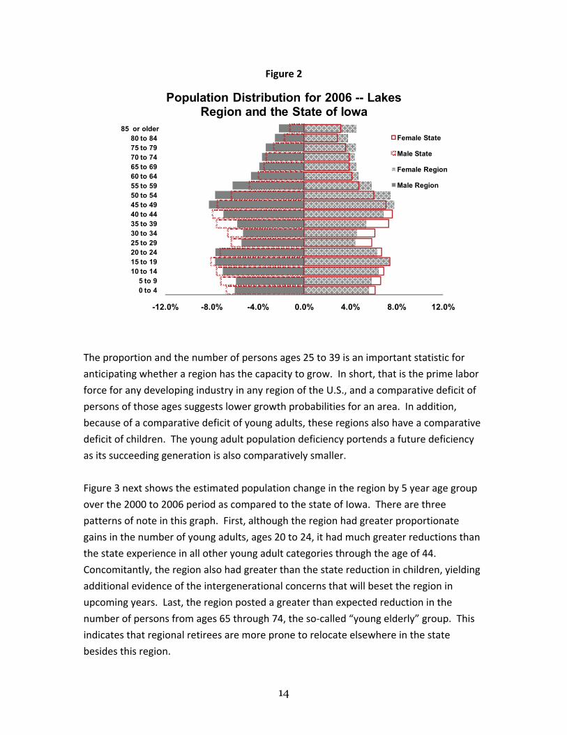
Figure 2
-12.0% -8.0% -4.0% 0.0% 4.0% 8.0% 12.0%
0 to 4 5 to 9
10 to 14 15 to 19 20 to 24 25 to 29 30 to 34 35 to 39 40 to 44 45 to 49 50 to 54 55 to 59 60 to 64 65 to 69 70 to 74 75 to 79 80 to 84
85 or older
Population Distribution for 2006 -- Lakes Region and the State of Iowa
Female State
Male State
Female Region
Male Region
The proportion and the number of persons ages 25 to 39 is an important statistic for
anticipating whether a region has the capacity to grow. In short, that is the prime labor
force for any developing industry in any region of the U.S., and a comparative deficit of
persons of those ages suggests lower growth probabilities for an area. In addition,
because of a comparative deficit of young adults, these regions also have a comparative
deficit of children. The young adult population deficiency portends a future deficiency
as its succeeding generation is also comparatively smaller.
Figure 3 next shows the estimated population change in the region by 5 year age group
over the 2000 to 2006 period as compared to the state of Iowa. There are three
patterns of note in this graph. First, although the region had greater proportionate
gains in the number of young adults, ages 20 to 24, it had much greater reductions than
the state experience in all other young adult categories through the age of 44.
Concomitantly, the region also had greater than the state reduction in children, yielding
additional evidence of the intergenerational concerns that will beset the region in
upcoming years. Last, the region posted a greater than expected reduction in the
number of persons from ages 65 through 74, the so‐called “young elderly” group. This
indicates that regional retirees are more prone to relocate elsewhere in the state
besides this region.
14

Figure 3
‐30.0% ‐20.0% ‐10.0% 0.0% 10.0% 20.0% 30.0% 40.0%
0 to 4 5 to 9
10 to 14 15 to 19 20 to 24 25 to 29 30 to 34 35 to 39 40 to 44 45 to 49 50 to 54 55 to 59 60 to 64 65 to 69 70 to 74 75 to 79 80 to 84
85 or older
Percentage Change
Age Group
Percentage Population Change by Age Group, 2000 to 2006
State of Iowa Region
The intergenerational change statistic, the smaller proportions of young people, is
demonstrated further in Table 2. From the 2000 to 2001 academic year through 2006‐
2007, the region suffered a 7.3 percent decline in school enrollment. Palo Alto had
more than twice the regional decline at 15.5 percent, with the lowest decline in Buena
Vista County. These numbers reinforce the preceding table and indicate that the fixed
cost of education are likely to be consumed by fewer students and paid for by a
declining number of taxpayers.
15

Table 2. School Enrollment in the Lakes Region School Year
2000‐2001 2006‐2007 Change Percentage Change
State of Iowa 492,022 483,122 (8,900) ‐1.8%
Buena Vista 3,810 3,750 (60) ‐1.6%
Clay 2,822 2,548 (274) ‐9.7%
Dickinson 2,800 2,668 (132) ‐4.7%
Emmet 1,944 1,727 (217) ‐11.2%
Palo Alto 1,839 1,554 (285) ‐15.5%
Region Total 13,215 12,247 (968) ‐7.3%
Components of Regional Population Change
When we study a region’s population, we are interested in the components of change.
There are only three components to area population change: births, deaths, and
migration. We can decompose population change into these elements to see which are
playing what parts in explaining area changes.
The overall performance of the region on these elements is displayed in Table 3. The
region’s total change of ‐1,537 persons is explained as follows. It had a natural change
of 491, net outmigration of 1,778, and 248 persons for whom estimates could not
account. Two of the counties, Pala Alto and Dickinson were in natural decline as there
were more deaths than births. The vast majority of natural change in the region is
attributed to Buena Vista County gain, and only Dickinson County had net inmigration.
Net outmigration consists of the sum of all international migration into the region and
all domestic migration to or from other states.
16

Table 3. Components of Population Change, 2000 to 2006
Components Buena Vista Clay Dickinson Emmet Palo Alto Region
Births ‐ 1,609 1,302 1,069 833 684 5,497
Deaths = 1,159 1,128 1,088 790 841 5,006
Natural Change 450 174 (19) 43 (157) 491
Migration (695) (696) 582 (554) (415) (1,778)
Residual (73) (49) (63) (37) (26) (248)
Total Change (320) (571) 500 (548) (598) (1,537)
The Labor Force
There is relatively strong alignment of the region’s overall labor force performance with
the state, as shown in Table 4. Through November of last year, the year‐to‐date
statistics indicated the regional unemployment rate was just 3.5 percent. Clay was
lowest at 3.1 percent, and Dickinson and Emmet were highest at 3.7 percent. By all
standard comparisons, these are relatively low unemployment rates.
Table 4. Labor Force Characteristics Through November 2007
Employed Unemployed Labor Force
Unemployment
Rate
State of Iowa 1,602,700 60,600 1,663,300 3.6%
Buena Vista 10,020 340 10,360 3.3%
Clay 9,850 310 10,160 3.1%
Dickinson 10,020 380 10,400 3.7%
Emmet 5,740 220 5,960 3.7%
Palo Alto 5,220 190 5,410 3.5%
Region 40,850 1,440 42,290 3.4%
Regional Jobs
Table 5 gives us the total number of jobs in the region as provided by the U.S. Bureau of
Economic Analysis. Jobs are counted where they are located, regardless of where the
job‐holder lives. There are newer numbers available from the Department of Labor, but
the patterns of change over time demonstrated here are instructive for this portion of
the report. During the 1990s the region enjoyed an annual rate of job growth similar to
the state and the nation. Although Palo Alto’s rate was half the regional average,
17

Dickinson’s was nearly twice as high, so there was a lot of variability within the region.
During the first half of this decade, however, the region stalled. The nation’s rate of
annual growth was half the previous decade, and Iowa’s rate was a fourth of its previous
rate. The Lakes region, however, is stagnant overall. Dickinson continues to lead the
region, but Palo Alto, Clay, and Emmet County posted declines over the period
measured.
Table 5. Total Jobs 1990 to 2005 Annual Rate of
Change
1990 2000 2005
1990 to
2000
2000 to
2005
US 139,380,900 166,758,800 174,249,600 1.8% 0.9%
State of Iowa 1,645,944 1,934,077 1,968,219 1.6% 0.4%
Buena Vista 12,021 13,553 13,745 1.2% 0.3%
Clay 11,093 12,707 12,314 1.4% ‐0.6%
Dickinson 9,231 12,783 13,481 3.3% 1.1%
Emmet 6,053 6,732 6,606 1.1% ‐0.4%
Palo Alto 5,346 5,786 5,429 0.8% ‐1.3%
Region Total 43,744 51,561 51,575 1.7% 0.0%
Figure 4 clearly shows the pattern of change in total jobs and people realized by the
region as shares of the state totals. Although both trended down together through
most of the 1980s and the 1990s, regional job shares increased in the current decade
while population continued its decline. The job share is now above the population
share. There are two explanations for this: (1) the region, compared to surrounding
areas is attractive for job creation and is able to rely on more incommuters than would
be expected, or (2) the region is adding jobs, but those jobs are not sufficient to offset
the population erosions. This latter consideration is often an indication that the wage
level of new jobs is, on average, below the regional average.
18

Figure 4
2.3%
2.5%
2.8%
3.0%
1980 1985 1990 1995 2000 2005
Percen
t of Iow
a Total
Lakes Region Job and Population Shares of Iowa Totals
Jobs
People
Figure 5 tracks the total rate of job growth for the U.S., Iowa, and the region over the
past two decades. In this graph, 1980 values equal 1 (or 100%), and the plots track
patterns of change since that origin. We see that the state and the region diverged
from the national pattern of change through the mid 1980s, and that the region then
followed the national pattern through the late 1990s. We also see that the pace of
growth since has slowed for Iowa and the region. Over the 25 years measured, the
nation’s jobs grew by 53 percent, the state’s jobs increased by 28 percent and the
region’s by 20 percent.
19

Figure 5
1.53
1.28
1.20
0.50
0.75
1.00
1.25
1.50
1.75
1980 1985 1990 1995 2000 2005
1980
= 1.0
Index of Job Change: 1980 = 1.0 (or 100 percent)
US
Iowa
Lakes Area
Worker Earnings
Figure 6 allows us to see what has happened to the average earnings of workers in Iowa
and in the region when compared to the U.S. averages. In 1980, the region’s workers
earned just over 80 percent of the U.S. average pay per job, while the state was at 90.5
percent. The state has eroded by nearly 10 percentage points since to 80.7 percent, but
the region’s share has eroded by nearly 15 percentage points to 65.7 percent. While the
state has lost ground to the nation, the region has also lost ground to the state.
Average earnings per worker are an important component of maintaining the livability
and desirability of a region. In general, workers migrate to where they feel they will be
able to maximize their earnings chances, to include appreciable gains in the values of
their net worth (as usually measured by housing investment and retirement
accumulations). Depressed regional earnings are generally a hindrance to business
development efforts. This may seem counter‐intuitive to some, but the situation usually
is this: an area with depressed earnings likely will be exporting its skilled labor to
regions with better earnings. Businesses that are sensitive to labor costs might seem to
be initially attracted to an area where the prevailing wage level is low. In fact, however,
firms will often find that the pool of workers in such areas has skill and education
deficiencies. In short, wages notwithstanding, workers go to where they can get a good
20

return on their labor, and firms go to where there are workers. This simultaneous
dynamic generally works against many rural economies and thwarts much of their
economic development initiatives.
Figure 6
90.5%
80.7%80.2%
65.7%
40.0%
60.0%
80.0%
100.0%
1980 1985 1990 1995 2000 2005
Percen
t of U
.S.
Wage and Salary Per Job as a Percentage of U.S. Average
Iowa
Lakes
Next, a few words about small businesses and entrepreneurship: In recent years, the
state of Iowa has posted the lowest rates of new firm startups in the nation, but it also
has posted the lowest rate of firm failures in the nation. The consensus among analysts
is that the state, its people and investors, tend to be highly conservative and careful
about starting new businesses.
The overall returns to small business ownership can be measured in a number of ways,
but the Bureau of Economic Analysis does measure both the incidence of nonfarm
proprietors (either sole proprietors or simple partnerships) and the annual income that
they generate. Those values are displayed in Figure 7 below.
The findings are dramatic. In 1980, the average Iowa nonfarm proprietor had an income
per proprietorship that was about 93.5 percent of the U.S. average. In the Lakes region,
that average was 86.1 percent. Those relative positions held until the 1980s when Iowa
and the Lakes region values plummeted. By 2005 the state average was just 66.6
percent and the percentage in the Lakes region fell to 54 percent. This erosion in
21

returns to nonfarm proprietorships is both puzzling and troublesome. It implies much
lower returns to entrepreneurship, which helps to explain the very low rate of business
startups.
It is likely that the data in Figure 6 help to explain just what is going on in Figure 7. If,
overall, average earnings are depressed in the state and generally considered
substandard, then workers and households must (1) increase the number of jobs that
are part of that household or (2) begin a side business to help supplement family
incomes. As the side business is a supplement to earnings and not the primary source of
earnings, then the averages are to be expected to be low. Still, the two sets of statistics
taken together are quite bothersome for the state as a whole and for this region in
particular.
Figure 7
93.5%
66.6%
86.1%
54.0%
25%
50%
75%
100%
125%
1980 1985 1990 1995 2000 2005
Percen
t of U
.S. A
verage
Nonfarm Proprietor Income Per Proprietor Compared to the U.S. Average
Iowa
Lakes
The upshot is that Iowa households have to work more jobs and more hours to maintain
their household income levels. This pattern is illustrated starkly in the following graph.
In Figure 8 the average number of nonfarm work hours per week per capita are
measured and compared to the U.S. average. Over the course of this decade, Iowans
have worked consistently more hours per capita than the national average and the gap
between Iowa and the U.S. is widening in recent years. In 2007 it is estimated that the
average hours worked per capita in Iowa were 10 percent greater. This graph actually
22

understates the situation. First, it does not include farm hours worked, an area where
Iowa has a competitive advantage over the nation. Those hours are not in the
numerator while the farm families are in the denominator. Second, Iowa has a higher
proportion of non‐working elderly than the nation which inflates its denominator.
Perhaps more noteworthy, though, has been the strong increase in the slope in recent
years compared to the U.S. There are no comparable data at the county level so we
cannot make estimates for the Lakes region.
Figure 8
13.0
14.3
11.5
12.0
12.5
13.0
13.5
14.0
14.5
2001 2002 2003 2004 2005 2006 2007
Hou
rs
Iowa and U.S. Average Weekly Hours of Work Per Capita
U.S. Iowa
23

III. Regional Industrial Summary
This section profiles the comparable size and broad industrial composition of the Lakes
area economy. Table 6 lists several measures of industrial activity. These data are
derived from an input‐output summary of the regional economy that was compiled by a
non‐governmental source.* The data are presented in concordance with the North
American Industrial Classification schema at the “2‐digit” level, which allows us to
identify the major sectors of the regional economy.
In 2006, according to this summary, there were 49,036 jobs in the region producing
$6.124 billion in industrial output. Industrial output is, roughly, the sales value of all
production by all industries and governments in the area. Payroll to workers in the
region was $1.32 billion, returns to sole proprietors were $277.3 million, payments
made to investors were $804.5 million, indirect tax payments to governments was
$185.8 million, and total value added, the sum of the preceding four categories, was
$2.59 billion. All manufacturing accounted for $2.45 billion of the region’s output,
followed by agriculture at $802.5 million. All governments came in a very distant third
in this category with $571.8 million in output value. The top five sectors for jobs were
manufacturing at 7,447, governments at 6,668, all agriculture at 4,384, health and social
services at 4,295, and accommodation and food services at 3,620.
* The data for this region were compiled by the Minnesota Implan Group, Inc. This company provides estimates of industrial data summarized down to the county level. These data are based largely on existing U.S. Bureau of Labor Statistics, Bureau of Economic Analysis, and Census Bureau data sets that are compiled annually or quinquennially by federal agencies. Gaps in data are filled using “clean and structure” techniques to estimate missing data by apportioning broad categorical remainders into categories where data were either missing or suppressed. As a consequence, some of the industrial details in more highly disaggregated tables are estimates.
24

Table 6. Summary Industrial Accounts for the Lakes Region, 2006 All financial amounts in millions + + + + =
Total
Industrial Output
Jobs Employee
Compensation Proprietor
Income
Other Property Income
Indirect Business
Taxes
Value Added
Ag, Forestry, Fish & Hunting 802.493 4,384 36.814 90.537 115.074 13.099 255.524
Mining 22.274 82 0.904 2.524 2.981 0.456 6.866
Utilities 95.692 229 15.874 3.062 36.045 10.044 65.025
Construction 265.184 2,458 72.436 25.918 13.435 1.455 113.245
Manufacturing 2,451.02 7,447 327.807 37.53 175.967 13.622 554.925
Wholesale Trade 214.764 1,687 68.133 12.96 31.789 31.765 144.647
Transportation & Warehousing 150.811 1,596 44.26 14.492 12.787 2.778 74.317
Retail trade 367.595 6,855 121.746 23.113 39.999 49.348 234.206
Information 86.88 543 16.131 0.44 9.405 2.615 28.591
Finance & insurance 203.27 1,155 50.36 4.488 79.123 2.891 136.862
Real estate & rental 120.938 1,340 7.277 13.017 47.429 13.968 81.691
Professional- scientific & tech 111.983 1,285 31.806 17.587 4.551 0.993 54.937
Management of companies 5.101 46 1.474 ‐0.002 0.395 0.03 1.898
Administrative & waste services 78.405 1,753 24.182 5.204 6.72 1.048 37.155
Educational 25.326 651 10.22 0.469 0.405 0.056 11.15
Health & social services 258.44 4,295 123.864 12.813 14.563 2.046 153.287
Arts- entertainment & recreation 30.459 671 7.256 2.203 3.802 1.704 14.965
Accommodation & food services 156.967 3,620 42.691 2.575 15.209 7.85 68.324
Other services 105.031 2,270 34.196 8.377 1.015 3.891 47.478
Government & non NAICs 571.796 6,668 283.819 0 193.779 26.096 503.694
Totals 6,124.42 49,036 1,321.25 277.306 804.473 185.755 2,588.79
Table 7 shows just how dominant manufacturing and agriculture were in the Lakes
region economy in 2006. Manufacturing was 40 percent of industrial output (the value
of gross sales), and agriculture followed at 13.1 percent. Output, however, is a crude
measure of industrial activity in a region. It is more appropriate to use either jobs or
value added to gauge the overall importance of industrial activity to a region and its
communities.
Using these more standard measures, manufacturing produced 15.2 percent of the
region’s jobs and yielded 21.4 percent of its value added. Agriculture produced 8.9
percent of jobs and 9.9 percent the regional value added. The second highest share of
value added was found in the government sector at 19.5 percent. Because the value
added percentage is above the jobs percentage in manufacturing, the returns of these
jobs to workers and to investors were comparatively higher than most of the remaining
sectors of the Lakes regional economy (wages to workers and payments to investors are
the bulk of value added). The retail sector is the second most prevalent industry in
terms of jobs at 14 percent but only generates 9 percent of value added. The worst
25

ratios of value added to jobs are found in entertainment and recreation,
accommodation, and all other services.
Table 7. Summary Industrial Accounts for the Lakes Region, 2006, as Percentages of Regional Totals
Total Industrial
OutputJobs
Value Added
Ag, Forestry, Fish & Hunting 13.1% 8.9% 9.9%
Mining 0.4% 0.2% 0.3%
Utilities 1.6% 0.5% 2.5%
Construction 4.3% 5.0% 4.4%
Manufacturing 40.0% 15.2% 21.4%
Wholesale Trade 3.5% 3.4% 5.6%
Transportation & Warehousing 2.5% 3.3% 2.9%
Retail trade 6.0% 14.0% 9.0%
Information 1.4% 1.1% 1.1%
Finance & insurance 3.3% 2.4% 5.3%
Real estate & rental 2.0% 2.7% 3.2%
Professional- scientific & tech 1.8% 2.6% 2.1%
Management of companies 0.1% 0.1% 0.1%
Administrative & waste services 1.3% 3.6% 1.4%
Educational 0.4% 1.3% 0.4%
Health & social services 4.2% 8.8% 5.9%
Arts- entertainment & recreation 0.5% 1.4% 0.6%
Accommodation & food services 2.6% 7.4% 2.6%
Other services 1.7% 4.6% 1.8%
Government & non NAICs 9.3% 13.6% 19.5%
Totals 100.0% 100.0% 100.0%
The preceding table allows us to gauge sectoral strength in the regional economy; Table
8 shows which counties accounted for which components of industrial activity in the
region. Buena Vista had 35 percent of the output, nearly 27 percent of the jobs, and
29.2 percent of the value added. Clay County had a quarter of all jobs and value added,
but only 20 percent of industrial output. Again, comparatively, areas where the value
added share exceeds the jobs share are areas where productivity is higher per job and
compensation is higher than the regional average. The gap between value added and
jobs is relatively small in all of the counties with only Buena Vista’s value added
percentage exceeding its jobs by a substantial margin.
26

Table 8. Industrial Summaries by County or Area
Summary all Counties
Total Industrial
Output JobsValue
Added Buena Vista 34.9% 26.8% 29.2%
Clay 20.0% 25.2% 25.1%
Dickinson 21.6% 24.1% 23.2%
Emmet 11.6% 12.0% 11.4%
Palo Alto 12.0% 11.8% 11.1%
Region 100.0% 100.0% 100.0%
Table 9 compares the major industrial values found in the Lakes region to those of the
state of Iowa. This table is very instructive and gives a good general idea of the region’s
comparative strengths and weaknesses vis à vis the state of Iowa. The first set of values
to understand are the column totals. These are “expected” values. They represent the
region’s total shares of state activity in the categories measured. The region had 2.4
percent of the state’s industrial output, 2.5 percent of jobs, and paid out 2.2 percent of
the state’s value added. These, for each column, are the expected values for the region.
Now that we know the expected values, we can look to where the region has categorical
strengths and weaknesses. Values in green are areas that were a half of a percentage
point than the expected values. Those in red shading are a half a percentage point or
more below the expected values.
Overall, broadly, the region has strengths in agriculture, mining, manufacturing, retail
trade, and accommodation industries. It has comparative weaknesses in transportation
and warehousing, financial and information industries, and in most of the professional,
health and social, and other service categories. All other sectors are, plus or minus,
relatively close to the expected values.
27

Table 9. Summary Industrial Accounts for the Lakes Region, 2006, as Percentages of State Totals
Lakes Region
Total Industrial
Output JobsValue
Added Ag, Forestry, Fish & Hunting 5.3% 3.4% 5.4% Mining 3.6% 3.0% 2.6% Utilities 2.9% 3.2% 2.6% Construction 2.2% 2.3% 2.1% Manufacturing 2.7% 3.2% 2.5% Wholesale Trade 2.0% 2.3% 2.0% Transportation & Warehousing 1.7% 2.0% 1.6% Retail trade 2.9% 3.0% 2.9% Information 1.1% 1.5% 0.9% Finance & insurance 1.0% 1.1% 1.2% Real estate & rental 2.2% 2.8% 2.3% Professional- scientific & tech svcs 1.5% 1.8% 1.5% Management of companies 0.2% 0.4% 0.2% Administrative & waste services 1.8% 2.0% 1.5% Educational svcs 1.4% 1.6% 1.1% Health & social services 1.9% 2.2% 1.9% Arts- entertainment & recreation 1.9% 1.9% 1.6% Accomodation & food services 2.9% 3.0% 2.8% Other services 2.2% 2.3% 2.0% Government & non NAICs 2.5% 2.6% 2.4%
Totals 2.4% 2.5% 2.2%
The preceding table gave a general, albeit aggregated, indication of regional competitive
strengths. Table 10 below gives a much more detailed indication of regional
specialization. It calculates a specialization index for each displayed category as
compared to the state of Iowa. If an industry scores a 1.0, then it is producing relative
to the total value in that category, at the state average level as a fraction of all
production. A value greater than 1.0 indicates specialization. A value less than 1.0
indicates an absence of specialization. In the table cells shaded in green indicate 25
percent more specialization than would be expected. Cells shaded red indicate 25
percent less than would be expected. Industries not in evidence in the region were
deleted. All other un‐shaded cells range from .75 to 1.25 in value and would be
considered within generally normal ranges for a region as compared to the state. This
table, by color, readily shows regional competitive advantages within the state (the
28

green areas), average areas (the unshaded areas), and areas where the region, overall, is
industrially under‐represented (the red shaded spaces).
This greater detail shows that indeed the region has a lot of specialization in all aspects
of agriculture. It also demonstrates the region’s strengths and deficits in manufacturing.
Food and food related processing is strong, as are textiles and printing along with
transportation and furniture manufacture. The region shows, compared to Iowa, deficits
in the proportion of many other manufacturing categories.
The region also demonstrates some strength in several retail categories. Part of this is
attributable to the distribution of trade centers, and part is attributable to the
preponderance of small towns with, relatively, small stores. In contrast, the region
demonstrates deficits in most information, financial, and service categories except for
nursing and residential care services and accommodations.
29

Table 10.
Lake Region Industrial Competitiveness Compared to the State of Iowa
Industry Output Jobs Value Added
Crop Farming 2.06 1.15 2.25
Livestock 2.36 1.50 3.23
Forestry & Logging 1.76 1.72 1.75
Fishing‐ Hunting & Trapping 2.91 2.76 3.47
Ag & Forestry 1.80 1.68 1.98
Mining 0.86 0.76 1.03
Mining services 0.67 1.62 0.52
Utilities 1.18 1.29 1.15
Construction 0.90 0.91 0.94
Food products 1.81 2.60 1.83
Beverage & Tobacco 0.03 0.04 0.02
Textile Mills 1.58 1.40 1.17
Apparel Mfg 0.02 0.02 0.02
Wood Products 0.99 1.10 0.95
Printing & Related 2.00 2.30 2.35
Petroleum & coal processing 1.66 0.47 2.75
Chemical Manufacturing 1.16 0.49 2.07
Plastics & rubber prod 0.12 0.14 0.12
Nonmetal mineral prod 0.46 0.59 0.43
Primary metal mfg 0.26 0.78 0.43
Fabricated metal prod 0.58 0.62 0.63
Machinery Mfg 1.01 1.19 1.09
Computer & other electronic 0.06 0.05 0.08
Electrical equip & appliances 0.07 0.14 0.05
Transportation equip 1.57 1.08 1.57
Furniture & related prod 2.04 2.94 1.74
Miscellaneous mfg 1.19 1.06 1.31
Wholesale Trade 0.83 0.93 0.90
Air transportation 0.15 0.19 0.01
Rail Transportation 0.21 0.20 0.23
Water transportation 0.14 0.24 0.08
Truck transportation 0.80 0.87 0.79
Transit & ground passengers 1.46 1.50 1.54
Pipeline transportation 0.68 0.65 0.73
Sightseeing transportation 1.74 1.51 1.89
Postal service 0.82 0.89 0.86
Couriers & messengers 0.42 0.57 0.40
Warehousing & storage 0.45 0.37 0.50
Motor veh & parts dealers 1.19 1.28 1.27
30

Table 10 (Continued)
Lake Region Industrial Competitiveness Compared to the State of Iowa Industry Output Jobs Value Added
Furniture & home furnishings 1.30 1.50 1.38
Electronics & appliances stores 1.02 1.33 1.11
Bldg materials & garden dealers 1.41 1.56 1.48
food & beverage stores 1.32 1.16 1.48
Health & personal care stores 0.81 0.83 0.87
Gasoline stations 1.57 1.26 1.71
Clothing & accessories stores 0.75 0.88 0.81
Sports‐ hobby‐ book & music stores 0.55 0.76 0.52
General merch stores 1.26 1.18 1.39
Misc retailers 1.48 1.66 1.61
Non‐store retailers 0.93 1.14 1.01
Publishing industries 0.30 0.60 0.30
Motion picture & sound recording 1.79 1.83 1.35
Broadcasting 0.65 0.76 0.60
Internet & data process 0.02 0.02 0.02
Credit inter‐mediation & related 0.10 0.11 0.11
Securities & other financial 0.43 0.42 0.47
Insurance carriers & related 0.11 0.22 0.16
Monetary authorities 1.10 1.05 1.20
Real estate 1.05 1.22 1.14
Rental & leasing 0.51 0.69 0.47
Professional‐ scientific & tech 0.64 0.71 0.68
Management of companies 0.10 0.14 0.07
Admin support 0.74 0.80 0.70
Waste mgmt & remediation 0.76 1.00 0.56
Educational 0.57 0.66 0.51
Ambulatory health care 0.77 0.81 0.83
Hospitals 0.42 0.47 0.40
Nursing & residential care 1.38 1.36 1.49
Social assistance 0.86 0.74 1.04
Performing arts & spectator sports 0.95 0.64 0.66
Museums & similar 0.80 1.17 0.65
Amusement‐ gambling & recreation 0.73 0.84 0.75
Accommodations 1.36 1.65 1.34
Food & drinking places 1.14 1.13 1.21
Repair & maintenance 0.95 1.10 0.91
Personal & laundry 0.88 1.00 1.00
Religious‐ grantmaking‐ & similar orgs 0.80 0.78 0.82
Private households 0.90 0.81 0.98
Government & non NAICs 1.02 1.06 1.08
31

IV. Characteristics of Industrial Production
Regional Input and Output Summaries
The regional economy for the five‐county area can be parsed into its constituent inputs
and outputs. In so doing we introduce readers to the elements of economic activity in
the region. All of these data come from an input output model of the regional economy
for 2006. That is the latest year for which estimates of the regional economy are
available. This data set, however, is very appropriate for the modern economy because
it does contain the recent additions of biofuels and casino operations to the region.
Total inputs in an economy always equal total outputs. Table 11 isolates the overall
inputs and outputs of the Lakes region. That amount is $6.124 billion. In producing that
output, regional industries made $3.54 billion in payments for production inputs, nearly
two‐thirds of which were imported. Next the region made payments to value added in
the amount of $2.6 billion. Payments to workers and proprietors combined form labor
income and represent 61.7 percent of all value added. Payments to investors and
property owners are 31 percent of value added, with the remaining amount going to
make indirect tax payments that are part of the production process in the region.
The table also lets us see how the outputs of the region are distributed. Local industries
purchase an estimated $1.21 billion of the region’s output, and the remaining $4.933
billion go to the final demanding sectors. The largest final demand category is exports
at 58.7 percent of the total, followed by regional households at 23.2 percent,
governments purchases are 9.7 percent of final demand, and the remaining 8.3 percent
go to inventory and capital.
This table is useful for understanding what makes a regional economy tick. Income in a
region is a function of all local consumption by households and industries plus all
exports, minus all imports.
An alternative characterization of inputs and outputs is displayed in Figure 9. It is based
on the data from Table 11 and gives a visual sense of the size of inputs and the size of
outputs from regional industries.
32
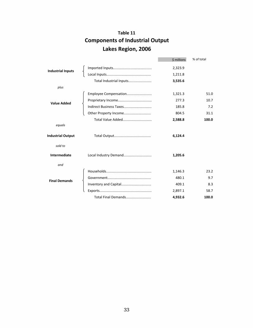
Table 11
$ millions % of total
Imported Inputs........................................ 2,323.9
Local Inputs.............................................. 1,211.8
Total Industrial Inputs........................ 3,535.6
plus
Employee Compensation.......................... 1,321.3 51.0
Proprietary Income................................... 277.3 10.7
Indirect Business Taxes............................. 185.8 7.2
Other Property Income............................ 804.5 31.1
Total Value Added.............................. 2,588.8 100.0 equals
Industrial Output Total Output...................................... 6,124.4
sold to
Intermediate Local Industry Demand............................. 1,205.6
and
Households............................................... 1,146.3 23.2
Government............................................. 480.1 9.7
Inventory and Capital............................... 409.1 8.3
Exports...................................................... 2,897.1 58.7
Total Final Demands.......................... 4,932.6 100.0
Components of Industrial OutputLakes Region, 2006
Industrial Inputs
Value Added
Final Demands
33

Figure 9 Components of Industrial Output in the Lakes Region
Imported Inputs
Locally Purchased Inputs
Employee Compensation
Proprietary Income
Indirect Business Taxes
Other Property Income
Local Industries
Households
$ 6,124 million
Government
Inventory and Capital
Exports
Payments by Industries Total Industrial Output Industry Sales
Measuring Output and Productivity
Table 12 re‐summarizes the basic components of industrial output for the region that
are already contained in Table 6 (in the previous section). It, however, compiles those
data on a per job basis as a measure of overall productivity. Productivity and rankings
are listed for output, value added, and earnings, a subset of value added. The standard
measure of productivity (or gross domestic product) is value added per job. By that
measure, the finance, insurance, and real estate sectors had the highest productivity,
followed by wholesale, and transportation and utilities. Services and retail trade yield
the lowest productivity. When that measure is applied just to the earnings levels of
workers, then the manufacturing sector has the highest measure, followed by wholesale
trade. All other services post the lowest measure of earnings per job, followed by retail.
Value added productivity is 96 percent of the state level. Earnings productivity is 92
percent of the state average. Earnings are the wages and salaries of workers, plus the
value of all work‐related benefits, plus the returns to sole proprietors.
34

Table 12
$ Per Job Rank $ Per Job Rank $ Per Job Rank
Agriculture and Mining......................................................... 184,676 2 58,753 5 29,283 9
Construction......................................................................... 107,842 7 46,053 7 39,998 5
Manufacturing...................................................................... 329,261 1 74,547 4 49,078 1
Wholesale Trade................................................................... 1 127,305 6 85,742 2 48,069 2
Retail Trade........................................................................... 1 53,640 9 34,176 9 21,138 10
Transportation and Utilities.................................................. 134,997 4 76,310 3 42,545 3
Communications and Information........................................ 160,002 3 52,656 6 30,517 7
Finance, Insurance, and Real Estate..................................... 130,047 5 87,667 1 30,141 8
Professional and Social Services........................................... 2 63,503 8 35,202 8 31,573 6
Other Services....................................................................... 46,334 10 20,761 10 15,545 11
Government.......................................................................... 3,4 42,452 4
Average, All Industries**................................................... 124,907 52,798 32,602
Average, State of Iowa...................................................... 4 117,583 54,845 35,496
Contributions by Industrial Sector
2 Private sector education and health services are included in the professional and social services group.
Lakes Region, 2006
................................................................................
3 Household and government enterprises engage in activities resembling those of business entities. Household transactions includeprivate households employing workers in activities primarily concerned with the operation of the household; transactions between
Average Output, Value Added, and Earnings per Job
Industry GroupOutput EarningsValue Added
1 Values for the wholesale and retail trade sectors reflect only their trade margins on the goods they purchase and resell.
households for used and secondhand goods; and the imputed rental value received by households for their owner‐occupied dwellings. Government enterprises include public utilities, passenger transit, and other public enterprises with characteristics of business entities.
sector. This may deflate the average output per job values in regions with relatively high concentrations of government employment.** All‐industry average output and value added per job includes values for household and government enterprises and the government
output per job and average value added per job values are not reported.
4 Government output and value added measures are not comparable with private industries; therefore, total government output,
Table 13 shows the composition of industrial outlays for each major industrial sector in
the region. This shows where regional industries make payments as part of their
production process and compares them to one another. Statewide averages are
included for comparison; however, differences from the state should be interpreted
with caution. The region, by virtue of its smaller size, is relatively more dependent on
imported inputs (38.7 percent) than the state (30.7 percent). Within the region, the
agriculture and manufacturing sectors are both more dependent on imported inputs
than other sectors. Payments to employment compensation represent relatively higher
fractions of inputs in the services and retail sectors. The finance and real estate sector
(FIRE) stands out with its relatively high proportion of input payments to other property
incomes (39 percent). This is due primarily to the heavy emphasis on farming and the
farmland rental payments accrue to that sector.
35
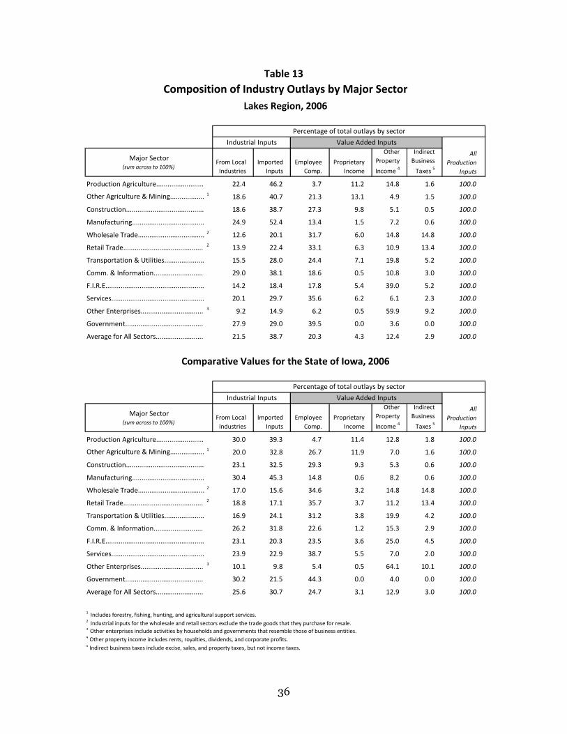
Table 13
From Local Industries
Imported Inputs
Employee Comp.
Proprietary Income
Other Property
Income 4
Indirect Business
Taxes 5
Production Agriculture......................... 22.4 46.2 3.7 11.2 14.8 1.6 100.0
Other Agriculture & Mining.................. 1 18.6 40.7 21.3 13.1 4.9 1.5 100.0
Construction......................................... 18.6 38.7 27.3 9.8 5.1 0.5 100.0
Manufacturing...................................... 24.9 52.4 13.4 1.5 7.2 0.6 100.0
Wholesale Trade................................... 2 12.6 20.1 31.7 6.0 14.8 14.8 100.0
Retail Trade.......................................... 2 13.9 22.4 33.1 6.3 10.9 13.4 100.0
Transportation & Utilities..................... 15.5 28.0 24.4 7.1 19.8 5.2 100.0
Comm. & Information.......................... 29.0 38.1 18.6 0.5 10.8 3.0 100.0
F.I.R.E.................................................... 14.2 18.4 17.8 5.4 39.0 5.2 100.0
Services................................................. 20.1 29.7 35.6 6.2 6.1 2.3 100.0
Other Enterprises................................. 3 9.2 14.9 6.2 0.5 59.9 9.2 100.0
Government......................................... 27.9 29.0 39.5 0.0 3.6 0.0 100.0
Average for All Sectors......................... 21.5 38.7 20.3 4.3 12.4 2.9 100.0
From Local Industries
Imported Inputs
Employee Comp.
Proprietary Income
Other Property
Income 4
Indirect Business
Taxes 5
Production Agriculture......................... 30.0 39.3 4.7 11.4 12.8 1.8 100.0
Other Agriculture & Mining.................. 1 20.0 32.8 26.7 11.9 7.0 1.6 100.0
Construction......................................... 23.1 32.5 29.3 9.3 5.3 0.6 100.0
Manufacturing...................................... 30.4 45.3 14.8 0.6 8.2 0.6 100.0
Wholesale Trade................................... 2 17.0 15.6 34.6 3.2 14.8 14.8 100.0
Retail Trade.......................................... 2 18.8 17.1 35.7 3.7 11.2 13.4 100.0
Transportation & Utilities..................... 16.9 24.1 31.2 3.8 19.9 4.2 100.0
Comm. & Information.......................... 26.2 31.8 22.6 1.2 15.3 2.9 100.0
F.I.R.E.................................................... 23.1 20.3 23.5 3.6 25.0 4.5 100.0
Services................................................. 23.9 22.9 38.7 5.5 7.0 2.0 100.0
Other Enterprises................................. 3 10.1 9.8 5.4 0.5 64.1 10.1 100.0
Government......................................... 30.2 21.5 44.3 0.0 4.0 0.0 100.0
Average for All Sectors......................... 25.6 30.7 24.7 3.1 12.9 3.0 100.0
3 Other enterprises include activities by households and governments that resemble those of business entities.4 Other property income includes rents, royalties, dividends, and corporate profits.5 Indirect business taxes include excise, sales, and property taxes, but not income taxes.
Comparative Values for the State of Iowa, 2006
Composition of Industry Outlays by Major SectorLakes Region, 2006
Industrial Inputs Value Added Inputs
AllProduction
Inputs
Percentage of total outlays by sector
Major Sector(sum across to 100%)
Major Sector(sum across to 100%)
Percentage of total outlays by sector
Industrial Inputs Value Added Inputs
AllProduction
Inputs
2 Industrial inputs for the wholesale and retail sectors exclude the trade goods that they purchase for resale.
1 Includes forestry, fishing, hunting, and agricultural support services.
36

Figure 10 itemizes the top 20 production inputs for the region and differentiates
between estimated imports and those that are regionally supplied. Livestock imports,
both into agriculture and into meat processing are a primary regional production input
at an estimated $596.1 million, with a substantial fraction expected to be supplied by
local producers. The vaguely defined wholesale sector is a distant second at $208
million, followed by real estate services, crops, and refined petroleum owing to the
region’s heavy dependence on energy inputs.
Figure 10
Total Inputs ($ millions)
Agriculture ‐ livestock..................................................... 596.1
Wholesale trade services................................................ 207.8
Real estate services........................................................ 171.6
Agriculture ‐ crops.......................................................... 121.0
Petroleum refineries....................................................... 114.9
Management of companies and enterprises................. 108.7
Other animal food manufacturing................................. 101.6
Truck transportation...................................................... 77.2
Iron and steel mills......................................................... 72.1
Other engine equipment manufacturing....................... 71.4
Pesticide and other agricultural chemical mfg............... 60.8
Soybean processing........................................................ 55.1
Motor vehicle parts manufacturing............................... 48.0
Banking and savings institutions and related................. 48.0
Agriculture ‐ other.......................................................... 45.4
Architectural and engineering services.......................... 43.9
Oil and gas extraction..................................................... 42.8
Telecommunications...................................................... 41.5
Miscellaneous professional and technical svc................ 35.9
Insurance carriers........................................................... 34.0
Lakes Region, 2006
Top 20 Inputs to Regional Industrial Production
- 200 400 600 800 $ millions
Assumed Imports Regionally Supplied
37

Figure 11 displays the region’s top 15 industries in total value added production. That
amount is divided into labor income, the earnings of workers and returns to proprietors,
into investors’ incomes (dividends, interests, and rents) and indirect payments to
governments. The labor income portion is very important because that aspect of value
added remains in the region and is most readily converted into household income.
Crop farming leads with $170 billion in value added. Next at $133 and $120 million
respectively are state and local government non‐education and education sectors.
Fourth is the banking sector. Manufacturing occupies the 5th, 6th, and 8th positions.
Sectors where it is clear that labor income is the preponderance of value added are
government, the meat packing industry, health practitioners, wholesale, food and
drinking places, and nursing care.
Figure 11
Value Added ($ millions) Total
Agriculture ‐ crops.......................................................... 169.8
State & local government non‐education...................... 133.1
State & local government education.............................. 119.8
Banking and savings institutions and related................. 109.0
Pesticide and other agricultural chemical mfg............... 90.2
Animal, except poultry, slaughtering............................. 88.9
Real estate services........................................................ 78.3
Farm machinery and equipment manufacturing........... 73.3
Agriculture ‐ livestock..................................................... 68.6
Offices of health practitioners........................................ 66.2
Merchant wholesale ‐ durable goods............................ 65.5
Merchant wholesale ‐ nondurable goods...................... 65.4
Power generation and supply........................................ 57.5
Food services and drinking places.................................. 48.0
Nursing and residential care facilities............................ 43.6
*Other Property Income + Indirect Business Taxes
Lakes Region, 2006Top 15 Industries Ranked by Total Value Added
- 50 100 150 200 $ millions
Investors & Govt* Labor Income
38

Top Regional Imports
Earlier it was shown that the region was estimated to have $2.32 billion in commodity
and service imports. Table 14 lists the estimated values of the top 15 imports into
production for the region. Animal imports at $305 million are three times the values of
the next categories of company and enterprise management, petroleum refineries,
animal food manufacturing, and real estate services.
A more detailed assessment of imports later in this study will allow for an investigation
of the possibility that import demand is sufficient to pursue the development of import
substituting industries. From this aggregated list, however, it is evident that many of
the commodities that must be imported into the region are specialized goods that
cannot be produced locally.
Table 14. Top 15 Commodities or Services Imported Into the
Lakes Region, 2006
(listed by industries in which they are produced)
Imports in
Commodity or Service $ millions
Animal production, except poultry and eggs........................................................... 305.2
Management of companies and enterprises........................................................... 103.9
Petroleum refineries................................................................................................... 102.1
Other animal food manufacturing............................................................................ 99.5
Real estate services..................................................................................................... 99.4
Wholesale trade services............................................................................................ 79.8
Iron and steel mills...................................................................................................... 72.1
Other engine equipment manufacturing.................................................................. 71.4
Soybean processing.................................................................................................... 54.2
All other crop farming................................................................................................ 44.4
Motor vehicle parts manufacturing.......................................................................... 43.9
Grain farming............................................................................................................... 36.1
All other miscellaneous professional and technical services................................. 35.4
Oil and gas extraction................................................................................................. 30.0
Insurance carriers........................................................................................................ 29.9
39

V. Identifying Regional Key Industries
An important objective of industrial targeting research is to help economic development
planners to zero‐in on an area’s production, trade, and service strengths and to assist in
identifying emerging industries. Some economic development planning is analogous to
a personal investment strategy where investors attempt, via research and experience,
to place their resources into investments that will balance their expectations for growth
against their respective tolerances for risk. An investor would not seriously think about
putting funds into a category that research indicated might not grow in the near future.
Smart investors would be careful about fads and bandwagons. Finally, investors would
move resources away from categories that were likely to decline. Economic developers
must think along the same lines. The mix of industrial opportunities is very much like a
mix of stock choices.
This analogy to economic development is apt, but only to a point. Regional economic
development planners are not in charge of, nor do they have the power to influence,
the whole regional economy. To pretend so would be silly, if not arrogant. Instead,
economic development practitioners have an opportunity to steer both public and
private investment dollars and activities into areas that may accomplish one of several
important economic development goals. For example, developers may wish to
Encourage the diversification of industrial production in an area to offset historic patterns to help move the regional industrial mix into the direction of the state or
national economy,
Capitalize on existing industrial strengths and use those strengths to leverage similar
industries or industries that link well with that historical base,
Nurture nascent industrial activity appearing to hold promise or further the
development of regional or sectoral niche industries,
Search for new firms that allow for more efficient utilization of existing private and
public infrastructure such as private and public transportation, storage, energy
production capacity, and municipal utilities. Regional education capacity could also
be considered in this instance.
40

Enhance the average earnings potential of regional labor force members and the
total incomes of the average regional household.
In all of these examples, the economic development planners ideally are using sound
industrial, labor force, and other economic research to inform their decisions. They are
not transforming the economy regionally, they are working to use scarce public
resources in manners that are efficient and offer the potential for desirable economic
and social outcomes.
The primary objectives of this portion of the analysis are three‐fold:
Clarify the region’s overall industrial strengths Identify industries that have a higher potential for locating in the region. In so doing, we hope to help identify industries that have comparatively attractive
economic development impacts to include,
Potential future growth
Wage values
Efficient utilization of existing private and public capacities
Ability to contribute to the regional tax base
The key industry methodology employed in this analysis looks at three main industry
selection criteria
Existing regional competitive advantages
Growth potential Evidence of emerging industries
Organizing the Primary Data Sets
There are two primary sources of data for our analysis. We are employing Minnesota
Implan data for our analysis of regional industrial structure and competitiveness. We
buy this data set annually, and the data we are currently using are for 2006. Implan
data have a high degree of detail and allow us to gain insights into regional industrial
composition that is not available from governmental sources. The other major source
for regional data is the Quarterly Census of Employment and Wages (QCEW)
administered by the Iowa Department of Workforce Development. They are also highly
detailed at the county level, and they provide valuable insights into industrial
41

compositions. Those data, however, must be managed carefully so as not to
unintentionally reveal proprietary information about firms in an area.
The first steps in conducting the targeted industry assessments for the region involved
setting two key analysis parameters: a reasonable time period for analysis and the level
of industrial detail. For the time parameter, we are primarily, regionally, only looking at
the 2000 to 2006 period as our era of contemporary change.
The selection of the appropriate level of industrial detail was influenced by structural
limitations of the data sets used for analysis. We are relying on Minnesota Implan data
as the foundation for our regional industrial social accounts. Those data were compiled
using a 1997 North American Industry Classification System (NAICS) basis, which has
minor differences from the 2002 NAICS coding structure currently in use by Iowa
Workforce Development and other state and federal agencies. Furthermore, the Implan
data are organized at several different levels of industrial specification. Some industries
are aggregated to the two‐digit NAICS level. In other instances the data set contains
four, five, and even six‐digit industrial classifications. Importantly and beneficial for our
purposes, Implan data are highly specific in the manufacturing sector.
Reconciling data set organizational structures required us to align IMPLAN data and the
QCEW data sets. A complete set of Implan industrial accounts in the region was
collapsed and aggregated at no greater than the NAICS five‐digit level, although several
industries were aggregated at a lower level. Next, the regional QCEW data sets for our
measurement years, 2000 and 2006, were aligned so that they matched the final
aggregations of the IMPLAN data set.
Key Industry Selection Process
With our resulting data sets, we looked at all industries in the region using the following
potential targeted industry selection criteria:
Firm size: There were 50 or more jobs in the industry region‐wide.
Regional specialization: The industries’ location quotients (LQ), a measure of local
industrial specialization, were greater than 1.50 in 2006.
Absolute employment change: There was evidence of a positive “shift” in
employment in an industry in excess of 25 percent, regardless of its location
quotient.
42

The first two selection criteria identify industries that have a significant presence in the
region (both in size and in specialization). Job changes calculated in the third category
allow us to differentiate industries that are competitive, stable, declining, and emerging.
Location quotients are a standard measure of an area’s industrial composition and
degree of industrial specialization. Using the U.S. as a basis for comparison, an area’s
location quotient (LQ) for an industry is simply the percentage of jobs in that industry
locally divided by the percentage of jobs in that industry nationally:
Regional jobs in industry i
_________________ Regional total jobs t
LQ = _____________________ U.S. jobs in industry I
__________________ U.S. total jobs T
A LQ of 1.0 means that an area has the same percentage of jobs in an industry as the
national average. A LQ < 1.0 means that there is a regional deficit of jobs in an industrial
category, the region does not demonstrate production specialization in that instance. A
LQ > 1.0 means that there is evidence of industrial specialization. Our cut‐off is 1.50.
That means, considering the national experience, industries in the region meeting this
criterion have 50 percent or more jobs than the national average would have suggested.
The higher the LQ in an industry in a region, the higher the assumed level of
specialization.
We also use job growth as a proxy indicator of LQ change. The LQs in our analysis were
calculated from the transformed Implan data set for the regional and U.S. economies.
We also calculated industrial job shifts for the 2001 to 2006 period using QCEW data. By
definition, industries with percentage changes in jobs in excess of the overall national
average rate of growth for that same industry over this period of time will have realized
an increase in their LQs. Industries with lower growth percentages will have realized a
decrease in their LQs. For the short period assessed, the percentage job changes
indicate change in industrial competitiveness.
43

Initial Selection Results
There are three major tables of industrial ratings resulting from our initial, targeted
industry selection criteria:
Agriculture and food processing industries. These industries all have more than 50
employees and location quotients (LQs) above 1.5.
Other manufacturing. These firms as well have more than 50 employees and LQs in
excess of 1.5.
All other industries. These industries meet the criteria for minimum jobs, but their
LQs might be below the cutoff value of 1.5. Instead, for those with lower LQs, they
demonstrated job growth of 25 percent or greater since 2000.
Within each table there are nine important industrial characteristic measures.
Value added. This is the same statistic as gross domestic product, and it is the
standard way in which industrial size and overall productivity are characterized in
the U.S. economy. This number is the amount in millions produced by the industry
in 2006
Location quotient. As explained above, the LQ is a measure of the region’s degree
of production specialization.
Local growth. This measure looks at the percentage of job growth since 2001 for
private wage and salary jobs. This helps us to identify emerging industries.
Local dispersion. This is a measure of the overall concentration employment in our
counties. Industries with low dispersion are concentrated in one or two counties.
Industries with high dispersion are more scattered about the region.
Local linkages. This measure is derived from the IMPLAN data set. It looks at the
ratio of jobs that provide inputs into the key industries. For example, if this ratio for
an industry was 1.3, that means that for every job in the key industry, there was
3/10th of a job in all of the supplying sectors. For every 100 jobs in the key sector,
then, there were 30 supplying jobs. The higher this measure, the greater the
industry’s job linkage to the regional economy.
44

Projected U.S. job growth annually. Expectations for future annualized growth in the industry at the national level were derived from Bureau of Labor Statistics data
sets for the U.S. for 2006 through 2016.
Projected U.S. output growth annually. Output is a measure of the sales value of all
production. This measure is of projected real or inflation adjusted growth for the
2006 through 2016 period.
Average earnings. These are the average earnings per job. They are analyzed as a percentage of the state average for that industry.
Export jobs. These are the jobs that are, statistically, producing for export to users outside of the region. The number of export jobs in an industry in the region is (1‐
1/LQ) X industrial employment.
The critical values for the last seven of these comparison indicators are presented below
in Table 15. In all cases, the least desirable indicators are coded red. Indicators that are
considered average are grey, and those coded blue indicate a better score. Readers can
quickly scan the tables to see which industries have the highest indicators by category,
or they can refer back to this table to identify the cut‐off values.
Table 15. Threshold Values for Key Industry Categories
Evaluation Criteria Low Medium High
Local Growth (private wage & salary jobs only ‐ from IWD) <0 <= 25% > 25%
Dispersion =1 0.5 ‐ 1 <.5
Local Linkages < 1.25 1.25 ‐ 1.5 > 1.5
Projected Annual Average Growth Rate < 0 < 1% > 1%
Projected Annual Average Growth Rate ‐ Output < 0 < 3% > 3%
Average Earnings < 87% 85‐100% > 100%
Export Jobs < 100 100‐500 > 500
Regional Key Industries
The regions key industries are grouped following this section in Tables 16 through 18.
Table 16 gives the agricultural and food processing key industries for the region. The
highest value added production (or GDP) is generated in meatpacking (slaughtering)
45

46
followed by grain and oilseed farming. Meatpacking also had the highest LQ of 44 of the
group followed by animal food manufacturing at 19, fish product manufacturing
(seafood) at 16, and hog production at 16. Only two of these industries, cattle farming
and agricultural services, posted strong job gains in the 2001 to 2006 period in excess of
25 percent, though six posted positive gains. Animal foods manufacturing and
meatpacking both posted job reductions, according the BLS statistics over this period.
Dispersion among the firms is mixed. All of the agricultural sectors are of course
dispersed, as too are the animal food manufacturers (this would include feed mills).
Two industries stand out as not dispersed, meaning the industries are in just one
county. Both poultry and fish processing have this characteristic, the remainder are
found in at least two counties in the region. The degree of local linkages is very high in
seven of the ten industries. This means that there are secondary jobs in the region that
are highly dependent on these industries. The only industry with a low linkage indicator
is the agricultural services sector because most of the inputs into that sector come from
external sources.
Projected U.S. job growth is disappointing in this group. All of the agriculture and ag
related sectors will have net negative job growth nationally, with only animal and
poultry processing slated for expansion. Agricultural services and all other food
processing are expected to grow, but at less than 1 percent per annum. Expectations
for national output growth are positive, however, for all 10 industries, with real output
gains in oilseed and grain farming expected to top 3 percent per annum in the future.
Average earnings in this category are superior to state averages in all of the agricultural
sectors and animal foods. They are average in the remaining food manufacturing with
the exception of all other foods where they are lower than the state average.
Last, are export jobs. In four of the sectors there are more than 500 jobs producing for
export – jobs dependent on external economic conditions, not local ones. Five have
from 100 to 500 export producing jobs, with only the cattle farming sector posting fewer
than 100 jobs producing for export.

Table 16. Lakes Re
gion
Spe
cialization Indu
stries: A
g an
d Food
Processing
Indu
stry
Value
Add
ed
Locatio
nQuo
tient
Local
Growth
Local
Dispe
rsion
Local
Linkages
Projected
U.S. Job
Growth
Projected
U.S.
Outpu
t Growth
Average
Earnings
Expo
rt
Jobs
Agriculture & Food Processing
Animal, excep
t pou
ltry, slaughtering
88.9
43.9
Grain farm
ing
84.5
6.6
Oilseed farm
ing
80.7
8.9
Animal produ
ction, excep
t cattle
and
pou
ltry and eggs
32.0
15.8
Poultry processing
29
.0
10.8
Other animal fo
od m
anufacturing
12
.6
18.7
All othe
r food
manufacturing
10
.5
12.0
Agriculture and
forestry sup
port activities
9.7
2.4
Seafoo
d prod
uct p
reparatio
n and packaging
8.1
16.4
Cattle ranching and farm
ing
7.5
0.8

Table 17 lists other, non‐food processing manufacturing key industries. There are 17 of them and they represent a range of production activity. The highest value added is found in the category of pesticide and other organic chemical manufacturing, at $90.2 million, followed by farm machinery and equipment at $73.3 million, and in a distant third other transport equipment at $41.3 million. Other transport equipment had the highest LQ at 108 followed by cylinder manufacturing at 44, and farm machinery and equipment at 40. High levels of local growth were found in ready‐mix concrete, fluid cylinders, ethanol (other organic chemical), surgical appliances, and wood kitchen cabinet manufacture. Six of the industries posted employment declines over the 2001 to 2006 period, with six posting growth, but less than 1 percent per year. Only farm machinery and equipment along with ready mix concrete demonstrated wide dispersion in the region. Concentration in just one county was recorded for eight industries, with the remaining seven found in at least more than one county. Strong local job linkages from suppliers was found in the chemical manufacturing sector, ethanol production, farm machinery and equipment, and other transportation equipment. Very low regional job linkages were noticed in five industries, with eight posting average industrial relationships. Industries with low linkages tend to have lower regional multiplier effects when they grow and when they decline. As is the case with manufacturing in general in the U.S., the projected job growth of these industries nationally is dire. Twelve are projected to decline, and the remaining five are expected to grow no more than 1 percent per year. Strong real output growth in the U.S. is expected in farm machinery and equipment, transport equipment, and in surgical appliances and supplies. The U.S. data post an expected real decline in output in agricultural chemical manufacturing and commercial printing. Output growth in all other industries is expected to be less than 3 percent per year. Readers will notice that the ethanol sector (other organic chemicals) is slated to lose jobs nationally and may have trouble reconciling that with the current ethanol boom in Iowa. The U.S. corn based ethanol industry will only offset through 2016 about a 10th of those projected losses, given the recently passed energy bill. Compared to other Iowa firms, earnings were much greater than the state average for printing, prefab wood buildings, chemical manufacture, and aluminum foundry work. Earnings were much below the state average for five industries and about average for seven. Farm machinery and equipment and upholstered furniture had export job estimates that exceeded 500. Six had export jobs amounts ranging from 100 to 500, and nine had export job values that were less than 100.

Table 17. Lakes Re
gion
Spe
cialization Indu
stries: O
ther M
anufacturing
Indu
stry
Value
Add
ed
Locatio
nQuo
tient
Local
Growth
Local
Dispe
rsion
Local
Linkages
Projected U.S.
Job Growth
Projected U.S.
Outpu
t Growth
Average
Earnings
Expo
rt
Jobs
Other Manufacturing
Pesticide and othe
r agricultu
ral che
mical m
anufacturing
90
.2
15.2
Farm
machine
ry and
equ
ipmen
t manufacturing
73
.3
39.6
All othe
r transportatio
n eq
uipm
ent m
anufacturing
41
.3
107.7
Uph
olstered
hou
seho
ld fu
rnitu
re m
anufacturing
35
.3
27.9
Commercial printing
30.2
3.3
Prefabricated woo
d bu
ilding manufacturing
17
.8
33.2
Fluid po
wer cylinde
r and actuator m
anufacturing
15
.2
43.6
Overhead cranes, hoists, and
mon
orail systems
10.5
34.0
Aluminum
foun
dries
8.8
11.8
Surgical app
liance and supp
lies manufacturing
7.5
3.1
Plate work manufacturing
7.3
5.3
Metal valve m
anufacturing
4.5
2.1
Woo
d kitche
n cabine
t and
cou
ntertop manufacturing
4.1
1.5
Other basic organic che
mical m
anufacturing
4.1
2.3
Ready‐mix con
crete manufacturing
3.9
1.6
Fabricated
structural m
etal m
anufacturing
3.3
1.9
Woo
d containe
r and pallet m
anufacturing
2.1
3.0

Table 18 contains the key industry list for the eleven other industries for the region.
From our data sources we discerned that power generation and supply (electric utility)
had the most value added in the region at $57.5 million, followed by truck
transportation, and non‐store retailers. Many of these industries did not make either
the minimum employment cut‐off or the LQ cut‐off but demonstrated growth sufficient
enough to gain our attention. Consequently, the highest LQ in the bunch is for other
accommodations at 3, the next highest 1.6 in truck transportation, followed by 1.5 for
power generation, nonstore retailers, and for artists and performers. Of these industrial
groups, six demonstrate strong job growth since 2000, and two, power generation and
nonstore retailers indicate declines.
Nine of the 11 industries are dispersed widely throughout the region with only the other
accommodations category (these are primarily tourism, camp ground, RV parks, and
other direct activities for visitors) and the independent artists and performers indicating
a concentration in one county. Among these firms, only the category of motion picture
and video production demonstrated a relatively high indirect jobs multiplier. Three had
average multipliers, and seven had multipliers in the lower range.
Only power generation is projected nationally to post declines in employment, and eight
of the group are in industries that are expected to grow strongly nationally. Similarly,
five of the industries are slated for strong U.S. real output growth in excess of 3 percent
per annum, and the remaining six are expected to grow also, but by less than 1 percent
per year.
Average earnings among the group are lower than the state averages in nine of the 11
categories. Above state‐level earnings were posted for sightseeing transport and for
other accommodations. Eight of the 11 industries have fewer than 100 export
producing jobs, and three have from 100 to 500 export producing jobs.

Table 18. Lakes Re
gion
Spe
cialization Indu
stries: A
ll Other In
dustries
Indu
stry
Value
Add
ed
Locatio
nQuo
tient
Local
Growth
Local
Dispe
rsion
Local
Linkages
Projected
U.S. Job
Growth
Projected
U.S.
Outpu
t Growth
Average
Earnings
Expo
rt
Jobs
All Other
Power gen
eration and supp
ly
57.5
1.5
Truck transportatio
n 40
.1
1.6
Non
store retailers
18.6
1.5
Hotels and motels, includ
ing casino
hotels
18.0
1.3
Services to
buildings and
dwellings
11.3
0.9
Other amusem
ent, gam
bling, and
recreation indu
stries
10.1
1.1
Scen
ic and
sightseeing
transportatio
n and supp
ort a
ctivities
for transpo
rtation
8.9
0.7
Other accom
mod
ations
2.3
3.0
Motion picture and vide
o indu
stries
1.6
0.9
Inde
pend
ent a
rtists, w
riters, and
perform
ers
1.2
1.5
Other edu
catio
nal services
1.0
0.3

VI. Import Substitution Opportunities
When we analyze industrial growth opportunities for a region, it is important to assess
all components of the regional economy. Thus far, we’ve looked primarily at regional
industrial specialization – areas where the economy is producing goods for exports and
are, therefore, key or basic industrial sectors. There are two other important
components to normal market activity in a region: overall regional consumption of
goods and services (by households, institutions, and private industry), and the amount
of imports that flow into a region.
It is instructive to think of an economy as a set of plusses and minuses. One of the ways
that we can configure our thinking about regional dynamics is to describe how money
accrues to the regional economy. In a very simplified vein,
Regional
Income =
All regional consumption (households, industries, and
institutions)
+ All export sales
‐ All import purchase
±
Other factors (investments and savings, taxation,
government transfers in, etc)
Regional economic development planners primarily work at stimulating (or replacing
lost) export sales. They generally can do very little about overall regional household
consumption patterns, but there are opportunities for an economy to increase regional
industrial consumption.
The mechanism for that possible enhancement is through the investigation of potential
import substitution by new local industrial production. Imports, according to the simple
table above, take income out of an area. By decreasing imports in (a minus) and
enhancing production of that commodity locally, you increase regional consumption (a
plus).
There are a variety of reasons that commodities are imported. For one, while Iowa
farmers like to believe that they feed the world, the vast majority of our household
foodstuffs are imported – other parts of the U.S. are much more efficient and

specialized in producing many of the necessary fruits, vegetables, and other food
products upon which we rely. A second reason is that there simply is not enough
demand density, either by industry or by households, to warrant the location of a
production facility in the region. As a third consideration, the region may not possess
requisite natural resources or other raw materials necessary to produce the commodity.
A good example of this would be petroleum or lumber products. Lastly, there may be
labor, infrastructure, or other preemptive market factors that rule out an area from
producing a commodity.
Still, it may be possible to expand industrial targeting in an area by investigating
industries that might have the potential to locate in a region. If import substitutes can
be identified, they have the potential to decrease sales leakages, add jobs, and enhance
regional income and job multipliers.
Criteria for Selecting Potential Substitutes
We are estimating the region’s imports of manufactured goods using the data produced
by our input‐output model of the region for 2006. That aggregated data set identifies all
the commodities expected to be used by all industries in the Lakes region. It also
estimates how much of that commodity demand is expected to be met by local
producers. The difference between total commodity demand and the regional
commodity supply is the commodity import value. We use following criteria to screen
and evaluate our data:
Total regional imports: We list regional industrial inputs for which estimated
imports exceeded $10 million in the most recent year for which data are available.
Import substitution firm potential: We determine the number of firms of average
national size that might be supported by the region’s total demand for the given
input. This value is obtained by dividing the total national sales for the industry
producing the input by the number of firms in that industry nationally. If the
average U.S. firm has sales of $20 million, then it would take $20 million of local
commodity imports to even consider attracting a new firm.
Regional specialization: There are two opportunities that present themselves. First,
if the industry does not exist in the region, then there is the potential of new
industrial recruitment. If the industry does exist, then that industry could expand ‐‐
53

existing firms could try to ramp up production. This measure tells us the presence of
the industry, and if present, whether the region already has a competitive
advantage.
Iowa targeted industry: Iowa has several broad categories of industrial targets designed to both build upon state existing strengths and to help diversify its
economic structure. This column simply identifies which of the import substitution
categories align with the state’s current industrial targets.
Projected U.S. job growth: Expectations for national industrial growth are included to help leaders figure out which industries are destined to expand in the U.S.
Projected U.S. output growth: Expectations for real growth in industrial output is also an important glimpse into the future. Industries that are destined to expand
real sales nationally would be more desirable than those that were not.
Table 19 lists the screening criteria for the indicators that are displayed in Table 20. In
most cases the least desirable position is coded as red, the average characteristic in
grey, and the superior position is coded blue. In the Iowa targeted industry column,
those industries that are not targets are coded grey as this is a dichotomous choice.
Table 20. Screening Criteria for Import Substitution Analysis
Low Medium High
Import Substitute Firm Potential < 1 firm 1‐5 firms > 5 firms Regional Specialization not present LQ <= 1.5 LQ > 1.5 Iowa Targeted Industry ‐ No Yes Projected U.S. Job Growth < 0 <= 1 % > 1 % Projected U.S. Output Growth < 0 <= 3 % > 3 %
54

Import Substitution Candidates
Table 21 lists the 42 estimated commodity imports into the region that were in excess of
$10 million in 2006. Before analyzing the table a few cautions are in order. It would be
a stretch to assume that these commodities and services might automatically be
candidates for industrial recruitment. Several of these industries may be disqualified.
For example,
Some industries may be undesirable or unlikely candidates in light of existing
national and international production locations and shifts in production locations in
recent years.
Resource‐dependent industries such as petroleum refineries require capital‐
intensive production facilities located near input sources that are not present within
the Lakes region.
Some of the region’s import flows represent highly specialized financial and real
estate services that are offered only in large, urban financial centers and could not
reasonably be produced within the region.
Other regional import flows through the wholesale trade sector represent highly
specialized goods that are demanded in insufficient quantities to merit a local
wholesaler. Our modeling system cannot differentiate the types of wholesale
goods.
Industries that clearly are not candidates for new industries due to an absence of
natural resources or other regional attributes are displayed in italics.
Referring to Table 21, we see that there are four categories that are near or exceed
$100 million in estimated regional inputs into production. The greatest of these is
management of companies and enterprises at $104 million, followed by refined
petroleum at $102 million, other animal food manufacturing at $100 million, and real
estate services at 99 million. In the management of companies category, firms that are
subsidiaries of other firms are assumed to be, in the main, managed by the parent firm.
Real estate services are also a particularly tricky category. It does not mean that there is
an overall deficit of real estate services in the region, only that much of real estate
services must be purchased by owners of real estate that do not live in the region. For
example, agricultural landowners that rent their land may live in another area of Iowa or
55

another state. The same goes for owners of commercial and rental housing property.
All of those private owners of real estate that is rented or leased in the region are part
of the real estate industry.
Of the 42 listed commodities, 17 were manufactured goods and eight were in service
areas that are valuable to all production in the region, to include management and
consulting, architecture and engineering, research and development, legal services,
advertising, data processing, employment services, and bookkeeping and accounting.
There were sufficient volumes of imports in 14 industrial categories to warrant at least 5
firms or more potential growth. There was not enough import volume, however, to
support even one new firm in 12 of the categories. The remainder could support from 1
to 4 firms.
Ten of the import substitution categories were for industries that did not exist in the
region. Six, on the other hand, were in industries in which the region already
demonstrated a strong competitive advantage by posting a location quotient in excess
of 1.5. The remaining firms had LQ values below 1.5.
Sixteen of the commodity groups were of goods produced by the state of Iowa’s
targeted industries. The remaining 26 categories were outside of the state’s current
industrial goals.
U. S job growth in excess of 1 percent per year is expected in 16 of the import
substitution categories, and job declines, nationally, are expected in 17. The remaining
9 industries have job growth projections that are less than 1 percent.
Finally, real gains in industrial output in excess of 3 percent per year are projected in 18
of the commodity groups, and declines in four. All others are expected to grow by less
than 3 percent per year.
Ten of the categories had three superior level ratings (a blue indicator), however only
one of which, animal foods manufacturing, was in a category that the region already
demonstrated a competitive advantage. Seven of the categories had at least three
inferior ratings (a red indicator or a grey in the targeted industry code), with phosphatic
fertilizer, steel mills, paperboard, and sawmilling posting four inferior indications.
56

Table 21. Import Substitution Candidates for the Lakes Region
Industry
Regional Imports ($mil)
Import Substitution
Firm Potential
Regional Specialization
Iowa Targeted Industry
Projected U.S. Job Growth
Projected U.S.
Output Growth
Management of companies and enterprises 103.9
Petroleum refineries 102.1
Other animal food manufacturing 99.5
Real estate 99.4
Wholesale trade 79.8
Iron and steel mills 72.1
Other engine equipment manufacturing 71.4
Soybean processing 54.2
Motor vehicle parts manufacturing 43.9
All other miscellaneous professional and technical services 35.4
Oil and gas extraction 30.0
Insurance carriers 29.9
Nondepository credit intermediation and related activities 28.8
Pesticide and other agricultural chemical manufacturing 23.8
Telecommunications 22.7
Other basic organic chemical manufacturing 22.6
Securities, commodity contracts, investments 22.5
Truck transportation 22.3
Management consulting services 19.9
Architectural and engineering services 19.2
Plastics packaging materials, film and sheet 18.9
Monetary authorities and depository credit intermediation 18.6
Paperboard container manufacturing 17.5
Scientific research and development services 17.3
Advertising and related services 17.2
Sawmills 15.8
Pharmaceutical and medicine manufacturing 15.1
Tire manufacturing 14.5
Rail transportation 14.1
Legal services 13.5
Data processing services 13.3
Semiconductors and related device manufacturing 13.0
Lessors of nonfinancial intangible assets 12.8
Ferrous metal foundaries 12.7
Automotive equipment rental and leasing 12.1
Plastics plumbing fixtures and all other plastics products 11.8
Air transportation 11.7
Metal valve manufacturing 11.4
Phosphatic fertilizer manufacturing 11.2
Warehousing and storage 10.5
Employment services 10.5
Accounting and bookkeeping services 10.1
57
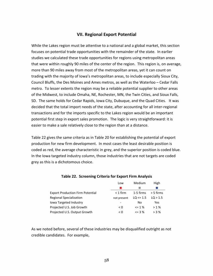
VII. Regional Export Potential
While the Lakes region must be attentive to a national and a global market, this section
focuses on potential trade opportunities with the remainder of the state. In earlier
studies we calculated these trade opportunities for regions using metropolitan areas
that were within roughly 90 miles of the center of the region. This region is, on average,
more than 90 miles away from most of the metropolitan areas, yet it can count on
trading with the majority of Iowa’s metropolitan areas, to include especially Sioux City,
Council Bluffs, the Des Moines and Ames metros, as well as the Waterloo – Cedar Falls
metro. To lesser extents the region may be a reliable potential supplier to other areas
of the Midwest, to include Omaha, NE, Rochester, MN, the Twin Cities, and Sioux Falls,
SD. The same holds for Cedar Rapids, Iowa City, Dubuque, and the Quad Cities. It was
decided that the total import needs of the state, after accounting for all inter‐regional
transactions and for the imports specific to the Lakes region would be an important
potential first step in export sales promotion. The logic is very straightforward: it is
easier to make a sale relatively close to the region than at a distance.
Table 22 gives the same criteria as in Table 20 for establishing the potential of export
production for new firm development. In most cases the least desirable position is
coded as red, the average characteristic in grey, and the superior position is coded blue.
In the Iowa targeted industry column, those industries that are not targets are coded
grey as this is a dichotomous choice.
Table 22. Screening Criteria for Export Firm Analysis
Low Medium High
Export Production Firm Potential < 1 firm 1‐5 firms > 5 firms Regional Specialization not present LQ <= 1.5 LQ > 1.5 Iowa Targeted Industry ‐ No Yes Projected U.S. Job Growth < 0 <= 1 % > 1 % Projected U.S. Output Growth < 0 <= 3 % > 3 %
As we noted before, several of these industries may be disqualified outright as not
credible candidates. For example,
58
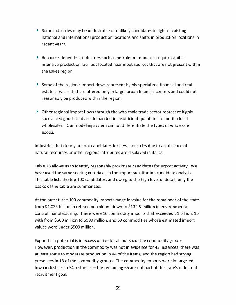
Some industries may be undesirable or unlikely candidates in light of existing
national and international production locations and shifts in production locations in
recent years.
Resource‐dependent industries such as petroleum refineries require capital‐
intensive production facilities located near input sources that are not present within
the Lakes region.
Some of the region’s import flows represent highly specialized financial and real
estate services that are offered only in large, urban financial centers and could not
reasonably be produced within the region.
Iowa industries in 34 instances – the remaining 66 are not part of the state’s industrial
recruitment goal.
Other regional import flows through the wholesale trade sector represent highly
specialized goods that are demanded in insufficient quantities to merit a local
wholesaler. Our modeling system cannot differentiate the types of wholesale
goods.
Industries that clearly are not candidates for new industries due to an absence of
natural resources or other regional attributes are displayed in italics.
Table 23 allows us to identify reasonably proximate candidates for export activity. We
have used the same scoring criteria as in the import substitution candidate analysis.
This table lists the top 100 candidates, and owing to the high level of detail, only the
basics of the table are summarized.
At the outset, the 100 commodity imports range in value for the remainder of the state
from $4.033 billion in refined petroleum down to $132.5 million in environmental
control manufacturing. There were 16 commodity imports that exceeded $1 billion, 15
with from $500 million to $999 million, and 69 commodities whose estimated import
values were under $500 million.
Export firm potential is in excess of five for all but six of the commodity groups.
However, production in the commodity was not in evidence for 43 instances, there was
at least some to moderate production in 44 of the items, and the region had strong
presences in 13 of the commodity groups. The commodity imports were in targeted
59

As many of the commodities are manufactured goods, the overall long term job
rospects are not good. Of the 100 commodity categories, 55 were expecting job
year,
t
hich the region had a level of specialization sufficient to assume some productive
anufactured commodities. The values
ange from $53.2 million in electric power and transformer manufacturing up to $3.215
high levels of specialization in 23 of the categories. That means the
egion has industries with LQ values in excess of 1.5. The remainder, by selection, range
ed
ational level is expected to decline in 21 of the commodity imports,
ut employment is expected to grow by more than 1 percent per year in 18 of the items.
p
declines at the national level, 24 are expected to grow by less than 1 percent per
and 26 are expected to exceed 1 percent per annum growth. Real industrial outpu
nationally is expected to decline in 13 of these commodities, grow, but by fewer than 3
percent per year in 47 of the items, and grow by more than 3 percent per year in 30.
Table 24 makes a second pass through the data and only selects commodity imports for
w
capacity. In this case we have chosen only the categories for which the region had at
least an LQ of .5, again, where an LQ of 1.0 means a region is self‐sufficient in
production. This table uses $50 million in statewide imports as the cut‐off, and
coincidentally there are 50 commodity groups.
Notably, seven of the top 10 groups are in nonm
r
billion in real estate services. Five exceed $1 billion in imports, and 14 are less than
$100 million.
The region has
r
from .5 to 1.5. Only 11 of the commodities in this grouping are part of Iowa’s target
industry definitions.
Employment at the n
b
Overall real output is expected to decline in just three, and it is expected to grow by
more than 3 percent per year in 15 items.
60
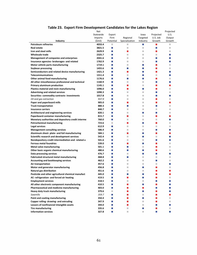
Table 23. Export Firm Development Candidates for the Lakes Region
Industry
Net Statewide Imports ($mil)
Export Firm
Potential Regional
Specialization
Iowa Targeted Industry
Projected U.S. Job Growth
Projected U.S.
Output Growth
Petroleum refineries 4033.4 Real estate 3821.5 Iron and steel mills 2629.9 Wholesale trade 2325.7 Management of companies and enterprises 2041.6 Insurance agencies‐ brokerages‐ and related 1762.9 Motor vehicle parts manufacturing 1719.1 Soybean processing 1455.6 Semiconductors and related device manufacturing 1421.3 Telecommunications 1311.4 Other animal food manufacturing 1176.6 All other miscellaneous professional and technical 1160.9 Primary aluminum production 1145.1 Plastics material and resin manufacturing 1096.0 Advertising and related services 1090.3 Securities‐ commodity contracts‐ investments 1017.8 Oil and gas extraction 937.9 Paper and paperboard mills 905.0 Truck transportation 880.3 Insurance carriers 840.7 Architectural and engineering services 820.1 Paperboard container manufacturing 815.7 Monetary authorities and depository credit interme 760.0 Petrochemical manufacturing 723.6 Legal services 612.9 Management consulting services 586.4 Aluminum sheet‐ plate‐ and foil manufacturing 584.1 Scientific research and development services 542.4 Nondepository credit intermediation and related a 541.6 Ferrous metal foundries 539.0 Metal valve manufacturing 501.1 Other basic organic chemical manufacturing 480.6 Data processing services 476.7 Fabricated structural metal manufacturing 468.8 Accounting and bookkeeping services 462.2 Air transportation 457.6 Motor and generator manufacturing 456.8 Natural gas distribution 451.6 Pesticide and other agricultural chemical manufact 445.0 AC‐ refrigeration‐ and forced air heating 419.5 Employment services 418.5 All other electronic component manufacturing 410.5 Pharmaceutical and medicine manufacturing 403.0 Heavy duty truck manufacturing 379.6 Sawmills 359.7 Paint and coating manufacturing 350.4 Copper rolling‐ drawing‐ and extruding 347.9 Lessors of nonfinancial intangible assets 344.0 Tire manufacturing 335.6 Information services 327.8
61
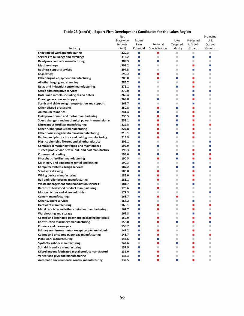
Table 23 (cont'd). Export Firm Development Candidates for the Lakes Region
Industry
Net Statewide Imports ($mil)
Export Firm
Potential Regional
Specialization
Iowa Targeted Industry
Projected U.S. Job Growth
Projected U.S.
Output Growth
Sheet metal work manufacturing 320.3 Services to buildings and dwellings 313.2 Ready‐mix concrete manufacturing 309.3 Machine shops 303.2 Business support services 297.5 Coal mining 297.3 Other engine equipment manufacturing 289.0 All other forging and stamping 285.7 Relay and industrial control manufacturing 279.1 Office administrative services 270.0 Hotels and motels‐ including casino hotels 269.4 Power generation and supply 268.8 Scenic and sightseeing transportation and support 265.7 Other oilseed processing 250.8 Aluminum foundries 241.4 Fluid power pump and motor manufacturing 235.5 Speed changers and mechanical power transmission e 232.1 Nitrogenous fertilizer manufacturing 229.8 Other rubber product manufacturing 227.8 Other basic inorganic chemical manufacturing 218.1 Rubber and plastics hose and belting manufacturing 215.9 Plastics plumbing fixtures and all other plastics 202.1 Commercial machinery repair and maintenance 195.9 Turned product and screw‐ nut‐ and bolt manufacture 195.3 Commercial printing 193.6 Phosphatic fertilizer manufacturing 190.5 Machinery and equipment rental and leasing 190.3 Computer systems design services 187.2 Steel wire drawing 186.8 Wiring device manufacturing 185.0 Ball and roller bearing manufacturing 183.1 Waste management and remediation services 181.7 Reconstituted wood product manufacturing 175.6 Motion picture and video industries 172.3 Cement manufacturing 168.7 Other support services 168.2 Hardware manufacturing 168.1 Metal can‐ box‐ and other container manufacturing 167.7 Warehousing and storage 162.8 Coated and laminated paper and packaging materials 159.0 Construction machinery manufacturing 158.0 Couriers and messengers 155.7 Primary nonferrous metal‐ except copper and alumin 147.2 Coated and uncoated paper bag manufacturing 145.7 Plate work manufacturing 144.6 Synthetic rubber manufacturing 142.6 Soft drink and ice manufacturing 137.9 Miscellaneous fabricated metal product manufacturi 135.0 Veneer and plywood manufacturing 133.3 Automatic environmental control manufacturing 132.5
62

Table 24. Export Firm Development Candidates for the Lakes Region – Moderate to High Regional Specialization
Industry
Net Statewide Imports ($mil)
Export Firm
Potential Regional
Specialization
Iowa Targeted Industry
Projected U.S. Job Growth
Projected U.S.
Output Growth
Real estate 3821.5 Wholesale trade 2325.7 Insurance agencies‐ brokerages‐ and related 1762.9 Soybean processing 1455.6 Other animal food manufacturing 1176.6 Truck transportation 880.3 Architectural and engineering services 820.1 Monetary authorities and depository credit interme 760.0 Legal services 612.9 Metal valve manufacturing 501.1 Other basic organic chemical manufacturing 480.6 Fabricated structural metal manufacturing 468.8 Accounting and bookkeeping services 462.2 Natural gas distribution 451.6 Pesticide and other agricultural chemical manufact 445.0 Tire manufacturing 335.6 Services to buildings and dwellings 313.2 Ready‐mix concrete manufacturing 309.3 Machine shops 303.2 Business support services 297.5 Office administrative services 270.0 Hotels and motels‐ including casino hotels 269.4 Power generation and supply 268.8 Scenic and sightseeing transportation and support 265.7 Aluminum foundries 241.4 Commercial machinery repair and maintenance 195.9 Turned product and screw‐ nut‐ and bolt manufactur 195.3 Commercial printing 193.6 Waste management and remediation services 181.7 Motion picture and video industries 172.3 Other support services 168.2 Plate work manufacturing 144.6 Fluid power cylinder and actuator manufacturing 127.3 Postal service 123.7 Miscellaneous wood product manufacturing 119.9 Animal‐ except poultry‐ slaughtering 113.4 Environmental and other technical consulting servi 99.8 Civic‐ social‐ professional and similar organizati 99.6 Transit and ground passenger transportation 94.1 Household goods repair and maintenance 92.9 Sand‐ gravel‐ clay‐ and refractory mining 86.1 Food services and drinking places 82.4 Farm machinery and equipment manufacturing 80.5 Prefabricated metal buildings and components 72.9 Gasket‐ packing‐ and sealing device manufacturing 72.6 Surgical appliance and supplies manufacturing 71.0 Independent artists‐ writers‐ and performers 61.3 Seafood product preparation and packaging 57.4 Industrial mold manufacturing 55.0 Electric power and specialty transformer manufactu 53.2
63

VIII. Regional Alignment with State of Iowa Targeted Industries
Methodology for the Targeted Industry Evaluation for the Lakes Region
The following assessment and evaluation has several parts and will take some
explaining. The goal of this section was to take a look at the state of Iowa’s targeted
industry groups and investigate the extent to which the regional industrial structure
both aligned with the targeted industry category or could potentially supply inputs to
those industrial targets. The point of this exercise was to evaluate the potential linkage
that the region has to the state of Iowa’s industrial targets as documented in the
Battelle Iowa Studies and Reports (http://www.iowalifechanging.com/studies.html).
Overall, the state’s industrial targets are classified as bioscience industries, advanced
manufacturing, or information technology.
This was an intricate estimating process that first identified the NAICS codes of the
industrial targets and then aligned those industries with our input output model. The
resulting classification yielded 157 distinct industrial sectors in our model. Next, for
simplicity’s sake, these industries were collapsed into 31 groups using the naming
conventions that are in the Battelle studies.
We evaluated the top 20 production input commodities into each of the industrial
targets using a national input output model in order to have a thorough sense of each
industry’s characteristics. We are looking at the total national production recipe for our
firms, both inputs that are produced domestically and those that are imported. Then
we identified whether industries in the region could supply those commodity inputs to
Iowa’s targeted industry firms were they to emerge. The region’s ability to supply
inputs to these industrial groups was scored by weighting the presence of firms that
produce that commodity in the region by the overall importance of that commodity to
the industrial target. In effect, the more important a commodity input, the higher the
score. The point of this analysis is to help regional planners identify their respective
abilities to potentially benefit locally from targeted industry growth elsewhere in Iowa,
let alone in the region.
Iowa Targeted Industry Alignment and Evaluation
In all, Table 26 below contains quite a bit of data. First, it identifies the overall industrial
composition of the major 31 groups as to whether they are advanced manufacturing
(AM), bioscience (BIO), or information technology (IT). In nine cases, there are firms in
64

the groupings that are in more than one category. As an example, ethanol production
(Chemicals, organic and agricultural) is classified as a bioscience and as an advanced
manufacturing industry – portions of the industry group fit into both taxonomies.
The 31 major groups are much more intuitively easy to grasp than the original 249
detailed categories gleaned from the Battelle research, and give a good sense of the
scope of industrial targets deemed important to Iowa’s overall long term economic
health. By way of evaluation, the first group is the degree of regional linkage
demonstrated by the region. Degree of local linkage is the weighted capacity of the
region to supply production inputs to the industrial targets, and is calculated relative to
the median linkage value for all 31 groups.
As before, we have determined the aggregate potential of the industries to generate
jobs in the future as gauged at the national level. We also look at real output growth,
where output is roughly the same as gross sales.
A new measure has been added that looks at net Iowa job shifts instead of actual job
growth. Despite overall national declines in manufacturing, Iowa’s share of
manufacturing jobs has been increasing in recent years. We measure here whether the
state is realizing share gains (or improvements in its national competitive position in the
industry of scrutiny). Next we evaluate wage level. These industries are evaluated at
the national level relative to all average earnings per job in all industries. Ideally, the
state would want to target industries that, nationally or regionally, paid higher than
average per job.
The last column measures the region’s occupational alignment with the industrial
targets. This is much like the evaluation of the production inputs, only in this instance
human capital is the input. For the schedule of necessary occupational needs at the
national level, an industry by occupation matrix was matched and aggregated to our
input output model. Next, the weighted occupational mix for the targeted industry
groups was compared to the region’s entire estimated occupational structure to
determine the degree to which it was in alignment with the targeted industry and its
primary supply change. This measure, in effect, determines whether there is a weak,
medium, or strong occupational alignment in the region with the production needs of
the targeted industry.
65

Taken together, these indicators help the region identify its potential to contribute
meaningfully to the state’s targeted industry goals, and, conversely, the set of target
industries’ overall potential contribution to job growth in the state.
Table 25 contains the evaluation criteria for Table 26. As before, the more desirable
position is coded in blue, the average position in grey, and the undesirable position in
red.
Table 25. Evaluation Criteria for State Targeted Industry Alignment
Low Mod High
Evaluation Criteria
Local Linkages (relative to median score for all 31 groups) <80% 80‐120% >120%
Projected U.S. Job Growth, 2006‐2016 < 0 <= 1% > 1%
Projected U.S. Output Growth, 2006‐2016 < 0 <= 3% > 3%
Iowa Competitive Job Shift < 0 <= 500 > 500
Wage Level Relative to U.S. All‐Industry Average < 100% 100‐150% > 150%
Occupational Fit (relative to median score for all 31 groups) <80% 80‐120% >120%
Of the 31 state targeted industry groups in Table 26, the region had a low level of supply
linkage in seven, and a high level in 12. Declines in jobs are expected in two‐thirds of
the industries at the national level, and strong gains in excess of 1 percent per year are
only expected in four. Strong real output growth at the national level, however, is
expected in 11 categories, and only one, printing and packaging, is expected to decline.
Iowa scores competitive job shifts in excess of 500 jobs when compared to the nation in
eight of the categories. This means, all other things equal, Iowa’s competitive position
in these firms is improving. Iowa’s competitive position vis a vis the nation deteriorated
in 14 categories. This means that Iowa is losing jobs to the rest of the nation or losing
jobs at a faster rate than the nation. In the remaining nine categories, the state has a
positive shift, but not in excess of 500 jobs. Much higher worker earnings can be
expected in six industrial categories, higher than the national average but less than 150
percent of the national average can be expected in 19 groups, and six industries in the
targeted grouping generally compensate below the average U.S. wage.
Last, the region’s occupational structure is misaligned with the production requirements
of aerospace and defense targets, industrial chemical production, and medical drugs
and devices. The region has strong occupational alignment with the production inputs
66

67
with five categories, to include ag services, construction components, printing and
packaging, communications and network services, and software and computer services.
In all other instances the region deviated about the median by a plus or minus 20
percentage points.

Table 26. Lakes Re
gion
Alignm
ent With State of Io
wa Indu
strial Targets
AM
BIO
IT
Targeted
Indu
stry Group
ing
Local
Linkages
Projected
U.S. Job
Growth
Projected
U.S. O
utpu
t Growth
Iowa
Compe
titive
Job Shift
U.S.
Wage
Level
Occup
ational
Alignm
ent
Aerospace and
Defen
se
Autom
ation Precision Machine
ry ‐ Bioscien
ce Focus
Autom
ation Precision Machine
ry ‐ IT Focus
Autom
ation Precision Machine
ry ‐ Other
Electron
ic & Com
puter H
ardw
are Co
mpo
nents ‐Sem
icon
ductors & Electronic
Compo
nents
Electron
ic & Com
puter H
ardw
are Co
mpo
nents ‐ C
ompu
ters & Periphe
rals
Electron
ic & Com
puter H
ardw
are Co
mpo
nents ‐ C
ommun
ications & M
edia
Electron
ic & Com
puter H
ardw
are Co
mpo
nents ‐ M
edia Recording
Equ
ipmen
t
Commercial & Indu
strial M
otor Veh
icles
Power Gen
eration Eq
uipm
ent
Indu
strial M
etal Processing
Digita
l & Electronic Devices ‐ Bioscien
ce Focus
Digita
l & Electronic Devices ‐ Other
Environm
ent C
ontrol Systems
Co
mmun
ications & M
edia Equ
ipmen
t ‐ Cable and
Wire
Active Ch
emical Agents
Polymers & Coatin
gs
Indu
strial Che
micals
Chem
icals ‐ O
rganic and
Agricultural
Med
ical Drugs & Devices
Agricultural Processing
Constructio
n Co
mpo
nents
Printin
g and Packaging
Agricultural Services
Engine
ering Re
lated Services ‐ Bioscien
ce Focus
Engine
ering Re
lated Services ‐ Other
Co
mmun
ications Network Services
Internet & Data Services
Med
ia Services
Software & Com
puter S
ervices
Hospitals & Labs
IX. An Occupational Evaluation for the Lakes Region
This next section addresses the region’s occupational structure. It is designed to give
the region a clear perspective on the kind of industries that it is attractive to by virtue of
the skill and knowledge base of its workforce. There are several innovative and
somewhat complicated calculations involved in this assessment, but there are other
components that are very similar to analyses done in previous sections.
In the first instance it must be emphasized that the occupational structure developed
for this assessment is based on the region’s industrial composition and the expected
staffing that those industries would require. We have not surveyed industries to gauge
occupations; instead we have identified employment in specific industries in the region
and then we applied national average industrial staffing components to the regional
industrial structure.
Like our previous assessments, we have compiled a location quotient indicator for the
region by different occupation. The location quotient is merely the percentage of
occupations in a sector locally of the total occupations locally as compared to the same
occupational percentage at the national level. From that analysis, we have chosen the
top 25 occupations, those where the region has strong location quotients, and the
bottom 25 occupations, those where the area has weak location quotients.
Next we compiled several qualitative measures for our occupational groupings.
1. Projected growth. The compounded annual growth rates in employment by occupation from 2006‐2016 are based on estimates for the United States from the Bureau of Labor Statistics. Occupations with projected employment declines are coded as “low” and are colored red, occupations with growth rates below the all‐occupation average of .99 percent are “moderate” and colored grey, and occupations projected to grow more rapidly than the average rates are “high” and coded blue.
2. Average earnings. Average annual wages by occupation for the United States were calculated using 2006 data from the Bureau of Labor Statistics. Occupations earning less than 85 percent of the all‐occupation average are coded as “low,” occupations between 85 and 100% of average are “moderate,” and occupations earning above the average wages are “high.”

70
3. Education. The education index measures the percentage of workers from 25 to 44 years of age with a 4‐year college degree or higher educational attainment. This measure may be used to evaluate the educational requirements of various occupations as well as the relative attractiveness of those occupations to young, college‐educated workers. The data were obtained from Occupational Projections and Training Data files from the Bureau of Labor Statistics. All occupations were ranked in order of the college‐educated worker percentages. In this report, occupations coded in red fall into the lowest quarter of all U.S. occupations. In these occupations, fewer than 8.7 percent of young workers have a college degree. Occupations coded in grey are in the second lowest quartile of U.S. occupations, with values between 8.7 percent and 18.6 percent. Occupations coded in blue are among the top half of U.S. occupations, ranked by percentage of young workers with a college degree.
4. Knowledge index and STEM knowledge index. The knowledge index scores are based upon a national data set that describes the type, level, and importance of knowledge typically required to perform jobs in different occupations. The information used here was obtained from the O*NET Version 12.0 database, maintained by the U.S. Department of Labor, Employment and Training Administration. The O*NET database contains data for more than 900 occupations and 33 knowledge areas including engineering and technology, mathematics, science, business and management, production, logistics, health services, education and training, and others.
Occupations in the national data set are rated by the level of knowledge (1‐7) and its importance (1‐5) in performing the job. Ratings are provided by individual knowledge area. For this report, scores across all knowledge areas were aggregated to construct an overall knowledge requirement score for an occupation. The scores for each occupation were obtained by multiplying the “level” scores by the “importance” score in each knowledge area, yielding a maximum overall value of 35 and a minimum of zero, and then averaging those resulting values across all knowledge areas. A subset of the knowledge areas was also used to construct a “STEM” index that describes knowledge requirements in science, technology, engineering, and mathematics. The occupations are color‐coded according to their national average knowledge requirements. Local differences in knowledge requirements are not captured within this analysis. Occupations falling in the bottom third of all U.S. occupations, as measured by their knowledge index, are coded in red. Occupations in the middle third are coded in gray, and occupations in the top third are coded in blue.

Table 27 summarizes the screening criteria and cutoffs established for the next two
tables.
Table 27. Evaluation Criteria for Occupational Analysis
Criteria Low Moderate High
Evaluation Criteria
Average annual U.S. employment growth, 2006‐
2016 <0 <= 0.99% > 0.99%
U.S. average annual earnings index < 85% 85‐100% > 100%
U.S. self‐employment index (all‐occupation
average is 7.5%) < 7.5% 7.5 ‐ 15% > 15%
% College degree or higher educational
attainment for workers ages 25‐44 < 9% 9 ‐ 19% > 19 %
Knowledge index < 3.4 3.4 ‐ 5.3 > 5.3
Science, Technology, Engineering, and
Mathematics (STEM) Knowledge index < 4.1 4.1 ‐ 5.9 > 5.9
Table 28 lists the region’s occupational strengths. All have location quotients based on
national figures that are greater than 1.0. Relative to Iowa, the region shows strengths
in five categories, weaknesses in four, and similar characteristics in 16. Of the region’s
strengths, though, eight are expected to post strong growth, another seven some
growth, but 10 are slated to decline in numbers nationally. Earnings are below 85
percent of the U.S. average in 17 of the occupations, and above 115 percent of the U.S.
average in just four. Three‐fifths of the occupations scored in the lowest group in terms
of the college index, while 17 were in the middle or higher group on the knowledge
index. The STEM statistics, however, is very low. Just four occupational strengths
scored in the higher group, and 16 scored in the bottom group.
Table 29 contains the region’s occupational deficits. The location quotient ranges from
the near‐average .9 to .3 for computer specialists. Disturbingly, when compared to
Iowa, the region is below the state average in all but one category. The importance of
these occupations nationally is indicated by the growth category – all are slated to grow
in number, and 14 are expected to grow smartly. Among these occupations, 16 have
very high average earnings, and six have low average earnings. Another 16 score
highest on the college index, and 13 score highest on the knowledge index. The STEM
score for this group, however, is really not that much better than the previous table: 11
score in the lowest group, and six are in the highest.

Table 28. Lakes Re
gion
Occup
ationa
l Evaluation ‐‐ Regiona
l Occup
ationa
l Spe
cialization
Occup
ation Group
Locatio
n Quo
tient
U.S.
Locatio
nQuo
tient
IA
Projected
U.S.
Growth
U.S.
Average
Earnings
College
Inde
x Kn
owledge
Inde
x STEM
Inde
x
Food
Processing Workers
7.7
Supe
rvisors, Farming, Fishing, and
Forestry Workers
4.0
Woo
dworkers
3.0
Farm
ing and Other Spe
cialized
Indu
stry M
anagers
2.6
Agricultural W
orkers
2.5
Printin
g Workers
2.0
Supe
rvisors, Produ
ction Workers
1.6
Other Produ
ction Occup
ations
1.5
Nursing, Psychiatric, and
Hom
e Health
Aides
1.4
Material M
oving Workers
1.3
Motor Veh
icle Ope
rators
1.2
Metal W
orkers and
Plastic W
orkers
1.2
Assem
blers and Fabricators
1.2
Retail Sales Workers
1.2
Supe
rvisors, Transpo
rtation and Material M
oving Workers
1.1
Supe
rvisors, Sales W
orkers
1.1
Vehicle and Mob
ile Equ
ipmen
t Mechanics, Installers, and
Rep
airers
1.1
Cooks and Food
Preparatio
n Workers
1.1
Other Foo
d Prep
aration and Serving Re
lated Workers
1.1
Textile, A
pparel, and
Furnishings W
orkers
1.1
Supe
rvisors, Foo
d Prep
aration and Serving Workers
1.1
Coun
selors, Social W
orkers, and
Other Com
mun
ity and
Social Service
Specialists
1.1
Material Recording, Sched
uling, Dispatching, and
Distributing Workers
1.1
Food
and
Beverage Serving Workers
1.0
Other Installatio
n, M
ainten
ance, and
Rep
air O
ccup
ations
1.0
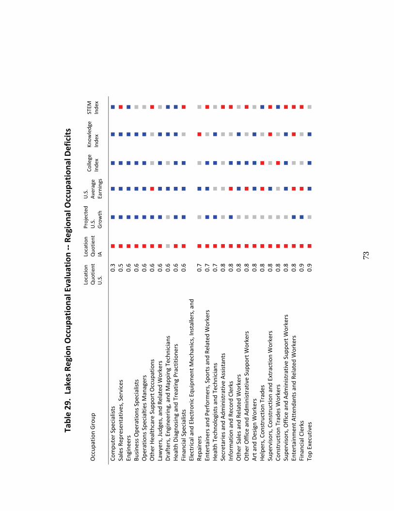
73
Table 29. Lakes Re
gion
Occup
ationa
l Evaluation ‐‐ Regiona
l Occup
ationa
l Deficits
Occup
ation Group
Locatio
n Quo
tient
U.S.
Locatio
nQuo
tient
IA
Projected
U.S.
Growth
U.S.
Average
Earnings
College
Inde
x Kn
owledge
Inde
x STEM
Inde
x
Compu
ter S
pecialists
0.3
Sales Re
presen
tativ
es, Services
0.5
Engine
ers
0.6
Busine
ss Ope
ratio
ns Spe
cialists
0.6
Ope
ratio
ns Spe
cialtie
s Managers
0.6
Other Health
care Sup
port Occup
ations
0.6
Lawyers, Jud
ges, and
Related
Workers
0.6
Drafters, Engineering, and
Mapping
Techn
icians
0.6
Health
Diagnosing and Treatin
g Practitione
rs0.6
Financial Spe
cialists
0.6
Electrical and
Electronic Equipm
ent M
echanics, Installers, and
Re
pairers
0.7
Entertaine
rs and
Perform
ers, Spo
rts and Re
lated Workers
0.7
Health
Techn
ologists and
Techn
icians
0.7
Secretaries and Adm
inistrative Assistants
0.8
Inform
ation and Re
cord Clerks
0.8
Other Sales and
Related
Workers
0.8
Other Office and Adm
inistrative Supp
ort W
orkers
0.8
Art and
Design Workers
0.8
Helpe
rs, Con
struction Trades
0.8
Supe
rvisors, Con
struction and Extractio
n Workers
0.8
Constructio
n Trades W
orkers
0.8
Supe
rvisors, Office and Adm
inistrative Supp
ort W
orkers
0.8
Entertainm
ent A
tten
dants and Re
lated Workers
0.8
Financial Clerks
0.9
Top Executives
0.9