Evaluating regional climate model estimates againstsite-specific observed data in the UK

M. Rivington & D. Miller & K. B. Matthews & G. Russell &G. Bellocchi & K. Buchan

Received: 27 June 2006 /Accepted: 6 November 2007 / Published online: 19 February 2008# Springer Science + Business Media B.V. 2007

Abstract This paper compares precipitation, maximum and minimum air temperature andsolar radiation estimates from the Hadley Centre’s HadRM3 regional climate model(RCM), (50×50 km grid cells), with observed data from 15 meteorological station in theUK, for the period 1960–90. The aim was to investigate how well the HadRM3 is able torepresent weather characteristics for a historical period (hindcast) for which validation dataexist. The rationale was to determine if the HadRM3 data contain systematic errors and toinvestigate how suitable the data are for use in climate change impact studies at particularlocations. Comparing modelled and observed data helps assess and quantify the uncertaintyintroduced to climate impact studies. The results show that the model performs very wellfor some locations and weather variable combinations, but poorly for others. Maximumtemperature estimations are generally good, but minimum temperature is overestimated andextreme cold events are not represented well. For precipitation, the model produces toomany small events leading to a serious under estimation of the number of dry days (zeroprecipitation), whilst also over- or underestimating the mean annual total. Estimatesrepresent well the temporal distribution of precipitation events. The model systematicallyover-estimates solar radiation, but does produce good quality estimates at some locations. Itis concluded that the HadRM3 data are unsuitable for detailed (i.e. daily time stepsimulation model based) site-specific impacts studies in their current form. However, theclose similarity between modelled and observed data for the historical case raises thepotential for using simple adjustment methods and applying these to future projection data.

Climatic Change (2008) 88:157–185DOI 10.1007/s10584-007-9382-9

M. Rivington (*) :D. Miller : K. B. Matthews : K. BuchanMacaulay Institute, Craigiebuckler, Aberdeen AB15 8QH, UKe-mail: m.rivington@macaulay.ac.uk

G. RussellSchool of Geosciences, The Crew Building, University of Edinburgh, West Mains Road, Edinburgh EH93JN, UK

G. BellocchiAgrichiana Farming, Montepulciano, Siena, Italy

1 Introduction

A major limitation in conducting site-specific climate change (CC) impacts studies is thedifficulty of determining daily data that are representative of the future climate for the site.Data currently produced by climate models driven by global and regional scale land, oceanand atmospheric processes aim to be representative at scales greater than those whereimpacts studies may be required, such as farms, catchments or ecozones. Though it ispossible to generalise about regional level impacts, using mean monthly data provided byglobal circulation models (GCM) and regional climate models (RCM), it is desirable toassess the impacts at individual locations using data with daily time steps. In order toproperly assess potential CC impacts (CCI) and the responses of the subject represented inthe impacts study, it is necessary to downscale from global to local scales (Droogers andAerts 2005). Spatial and temporal differences between the coarse scale GCM and RCMdata and the fine scale requirements of site-specific CCI, particularly for natural systems, isseen as a major limitation on the utility of such studies (Zhang 2005). Estimates ofalternative future climates derived from GCMs are associated with both significant scenariouncertainty (Jenkins and Lowe 2003) and modelling uncertainty (Murphy et al. 2004).Examples of scenario uncertainty include greenhouse gas emissions, economic andpolicy environment and population growth. Modelling uncertainty includes factors suchas uncertainty about model parameter values and errors resulting from model structure,both of which are reflected in the quality of individual weather variables. Moberg andJones (2004) stress the importance of knowing how well RCM’s estimate the presentclimate in order to interpret projected data for future scenarios. It can therefore be arguedthat the principal limitation in assessing CC impacts and adaptation strategies, is that theuncertainties in the climate model estimates, arising from either scenario and/ormodelling uncertainty are either unquantified or so large that meaningful conclusionsshould not be drawn from them. However, quantifying the modelling uncertainty for thepast climate becomes feasible by comparison between the models’ hindcast estimateswith observed data. This provides indications as to how, where and when biases in futureprojections may appear, and importantly either what adjustments could be made to correctthem, or how CCI outputs should be interpreted when the degree of uncertainty in datainputs are known.

Whilst RCMs are run for long time periods (i.e. hundreds of years) at fine time-scales(i.e. 30 min steps), and representing processes at a range of spatial scales, disseminatedoutput data is generally in an aggregated form and presented as daily estimates for past (i.e.1960–90) and future projections at set time slices (i.e. 2070–2100). Whilst the RCM aim torepresent the climate at the regional scale, the estimates for each cell within the model(typically 50×50 km grid cells) aim to be representative of the mean weather conditions forthe mean topographical and geographical characteristics within it. As such, it is beyond theRCM design remit to produce hindcast data identical to that for specific locations withineach cell. That said, it would be reasonable to expect that the RCM hindcast data at the gridcell scale would be ‘characteristic’ of observed data from ‘typical’ individual sites withinthe cell (i.e. having variables with similar temporal distribution patterns and value ranges).Where cells contain large topographical diversity however, it may be expected that datafrom meteorological stations at the extremes of that diversity are unlikely to show closesimilarity with modelled data. Any discrepancies will be partially due to the site and celldiffering in terms of topography, altitude, aspect or distance to the sea. Differences may alsobe attributable to the RCMs inability to adequately represent a particular cell due tonecessary assumptions or simplifications within the RCM modelling process.

158 Climatic Change (2008) 88:157–185

Improving the quality of daily weather variable estimates for future scenarios is vital inorder to better understand how biogeochemical processes will function under new climateconditions. If appropriate CC mitigation strategies are to be developed, for example inmanaging land uses to reduce greenhouse gas (GHG) emissions and increasing carbonsequestration, it is essential to be able to predict reliably the dynamic responses (spatial andtemporal) of the key biogeochemical processes. Many CCI studies will take the form ofpredictive modelling experiments, where simulations use RCM data as inputs. Unless errorsand other uncertainties in modelled weather data can be identified and quantified, thereliability and utility of the projections and use within CCI will be less certain. Governmentstrategic plans to cope with CC would hence be based on potentially incorrect evidencefrom impacts studies.

In this paper we compare the Hadley Centre’s RCM HadRM3 hindcast estimates ofprecipitation, maximum (Tmax) and minimum (Tmin) air temperature and total downwardsurface shortwave flux (direct and diffuse solar radiation, MJ m2 day−1), here referred to assolar radiation (So), with observed data from 15 meteorological stations in the UK for theperiod 1960–90 (Fig. 1.). For the reasons given earlier, we expect there to be differencesbetween the two data sets, as this is not a ‘like with like’ comparison, rather a ‘grid withpoint’ one. However, if the differences are conservative, they can be used to identifypotential adjustments to future grid cell projections, and provide information as to howerrors may appear when used in CCI studies. It is argued that it is necessary to assess thequality of the modelled climate estimates in advance, in order to determine the uncertaintythat will be introduced to any CCI study. If the assumption is made that the same modellingerrors existing in estimates of the past climate will also be present in future climateprojections, it is possible to appraise the usefulness of the future estimates, and potentiallyadjust biases using appropriate methods. Once these steps have been taken more reliableCCI studies should be possible.

2 Related research

Studies have sought to assess the performance of GCMs and RCMs at a range of spatial andtemporal scales (i.e. Peng et al. 2002; Antic et al. 2006). However, to date little work hasbeen done to compare RCM hindcast estimates with site-specific multiple variable observeddata (Moberg and Jones 2004). Exceptions include Bell et al. (2004), who performed amodel versus observed validation exercise as part of a larger study of growing seasonlength, extreme temperatures and precipitation in California. Long term data from 16stations were compared with 15 years of modelled data from a modified version ofRegCM2, for sites where the actual and modelled elevation differed by no more than100 m. These authors concluded that the RCM was able to make good estimates of seasonaltemperature and precipitation. One limitation of this study was that temperature basedassessments were distorted by the need to use proxy values for maximum and minimumtemperature (the model output values at midnight and midday, rather than providing theabsolute daily values). This indicates the need for careful consideration of what and howdata from RCMs are output and archived.

Moberg and Jones (2004) tested the HadRM3P model (closely related to the HadRM3assessed here) estimates of daily maximum and minimum near-surface temperatures for theperiod 1961–90 for 185 meteorological stations across Europe. The analysis was primarilybased on the model-minus-observed values for mean annual and seasonal temperaturedifferences, though results for daily differences (forming the annual temperature cycle)

Climatic Change (2008) 88:157–185 159

were given for six locations. These authors found large spatial variations in the ability of themodel to reproduce the historical weather well. It performed well in the UK and some otherlocations between 50 and 55°N, with differences generally being ±0.5°C, but other areasshowed differences of up to ±15°C. This study provided valuable information about the

Fig. 1 Meteorological stations providing observed data and the position of their associated HadRm3 50×50 km grid cell, with the station and mean cell elevations (m a.s.l.)

160 Climatic Change (2008) 88:157–185

degree of spatial variability in the quality of mean annual and seasonal temperaturedifferences at the regional scale, but did not cover site-specific multiple variable assessment.

Studies have compared estimates with observed data for individual weather variables atlarger spatial and temporal scales. For example, Mearns et al. (1995) assessed the quality ofestimates of precipitation by RegCM for a 42 month period. They stressed the importanceof models being able to reproduce the frequency and intensity of precipitation events, notjust the daily means. They also highlighted the limitations of statistical analysis of data setsfor periods of only a few years. Evans et al. (2005) tested four RCMs over a period of twoyears at a site in Kansas, USA, and found no clear distinction in performance between themodels, which all had positive and negative attributes. Fowler et al. (2005) tested theHadRM3 RCM for extreme rainfall events at 204 sites in the UK. Although the modelprovided good estimates of return periods for up to 50 years, it exaggerated the west to eastrainfall gradient, leading to overestimations in some higher elevation western areas, andunderestimation in eastern rain shadow areas.

RCM estimates have been compared with regional scale aggregations of observed data(i.e. Frei et al. 2002; Huntingford et al. 2003), or for time scales greater than individual days(i.e. Vidale et al. 2003). In testing the Rossby Centre Atmospheric RCM, RCA2, Jones etal. (2004) found that the model tended to overestimate the number of small precipitationevents, which impacted on surface temperatures and cloud-radiation interactions. Differ-ences are not only found for temperature and precipitation. Kim and Lee (2003) found thatsurface insolation was generally overestimated in an eight year hindcast simulation for theWestern USA with the differences being smaller over land than over the sea.

2.1 Importance of daily site-specific data

As many biological and chemical processes can only be studied effectively at a scale of afew hectares or less, there is a need to measure or otherwise provide weather data for theexact location (Hoogenboom 2000). However, policy makers are typically concerned withthe outcomes of key elements such as production, i.e. crop yields, and processes like GHGemissions, soil water balances and carbon sequestration, at regional (Holman et al. 2005),national (Sperow et al. 2003) or even supranational (Nijkamp et al. 2005) scales. Thereliability of estimates of such process outcomes, however, depends on robustlyparameterised relationships between the driving climatic variables and the outcomes ofinterest whilst incorporating anthropogenic factors such as adaptations of managementregimes (Rivington et al. 2007). Without site- or plot-specific data, unquantifieduncertainties are introduced into CCI studies and projections, making decisions based onevidence from such studies as either unreliable, or if the uncertainties are unrecognised,introduce biases that lead to erroneous decisions being made.

The uncertainty introduced into systems-model estimates due to the weather data sourcecan be significant (Rivington et al. 2006). Nonhebel (1994a) found that inaccuracies insolar radiation measurement of 10% and of daily temperature of 1°C in data used within acrop simulation model resulted in yield estimation errors of up to 1 t ha−1. Maintainingmeteorologically appropriate, synchronised relationships between individual weathervariables is essential for models that represent entities with non-linear responses to drivingvariables such as biological systems (Nonhebel 1994b) and hydro-chemical processes(Soulsby 1995; Creed et al. 1996). Thermal time accumulation, which depends not only onthe mean daily temperature but the difference between daily maximum and minimumtemperatures, is the key driver of plant and insect phenological development (Arnold andMonteith 1974; Jarvis et al. 2003, respectively). Systematic errors in the estimation or

Climatic Change (2008) 88:157–185 161

synchronisation of either Tmax and Tmin will result in predictions of either faster (earlier) orslower (later) development, with corresponding impacts on associated management (i.e.crop) or behavioural (i.e. plant–insect–predator) responses.

While the examples above are drawn from the agro-climatic rather than climate changeliterature, it seems reasonable to draw conclusions that, when using estimates of futureclimate derived from RCMs, researchers should be as concerned with issues of drivingvariable data quality. Hindcast RCM data provide a unique opportunity to assess the natureof the uncertainty introduced to CCI studies, particularly systems models’ predictions bythe use of RCM rather than site specific information.

3 Materials and methods

Observed precipitation (mm), maximum (Tmax) and minimum (Tmin) air temperature (°C)and total downward surface shortwave flux (direct and diffuse solar radiation, So, MJ m2

day−1) data for the period 1960–90 were provided by the British Atmospheric Data Centre(BADC 2005) for 15 meteorological stations in the UK (Fig. 1). The criteria for selection ofsites was that their data record contained the maximum number of complete years for allweather variables, and were sufficiently geographically dispersed to give a reasonablespatial representation of the UK, but also did not exist at the extremes of topography withineach cell. The number of sites available for assessment was limited by the availability of Sodata. Carnwath, despite not having So data, was included as it is a site of on-going CCImodelling (paper in preparation). Observed data for precipitation, Tmax and Tmin, and Sowere compiled within an Oracle database, with errors, duplicates and anomalies in theoriginal data being identified and corrected during the database loading process. Missingobserved values were filled using a search and optimisation method (LADSS 2007).

Modelled data used in this assessment is based on the hindcast simulations of the HadleyCentre’s HadRM3 RCM, as used in the UKCIP02 climate change scenarios report for theUK (Hulme et al. 2002). As an initial condition ensemble, five hindcast simulations(starting from 1860) were produced by the HadRM3 in order to establish the 1960–90climate normal period ‘baseline’ against which future projections were compared in theUKCIP02 report. Each hindcast simulation varied slightly in their starting conditions, butatmospheric CO2 and other GHG concentrations were varied to match the historicalconcentrations. Future projections of GHGs, as per the Special Report on EmissionsScenarios (SRES; IPCC 2000) were not applied until after 1990. This paper assesses two ofthe hindcast simulation data sets that were used to compare with the SRES A2c (medium-high) and B2 (medium low) future GHG emissions scenarios used in the UKCIP02 report.These two hindcast data sets are herein referred to as the A2cIRH and B2IRH, where IRH isthe initial realisation hindcast (observed historical GHG concentrations). As such, this paperassesses only two examples of the hindcast configuration of the HadRM3. The A2cIRH andB2IRH (1960–90) data were also provided by the BADC.

Daily climate data for each variable were derived from the HadRM3 archive for 50×50 km grid cells (the extent of each RCM cell used is shown in Fig. 1). Each meteorologicalstation was matched with its corresponding cell except in two cases where the stations werewithin 2 km of the cell boundary (Auchincruive and Eskdalemuir), in which case theopportunity was taken to use the closest neighbouring RCM cells for comparison as well.

The hindcast data produced by the RCM do not attempt to recreate synoptic conditionsfor specific locations or years in the period 1960–90. Instead, the RCM outputs are similarto those from weather-generators such as LARS (Semenov 2002) and CLIMGEN (Stöckle

162 Climatic Change (2008) 88:157–185

et al. 1999), in that they consist of time-series of data with the correct statistical propertiesincluding correlations between variables. The RCM outputs represent the 50×50 km gridcell as a whole rather than a specific site within it. RCM do not aim to reproduce the actualweather for a specific day or year in the past, rather they aim to produce values of a variablethat are representative (by magnitude, variability and synoptic synchronisation) of a day atany specific time of year. As such direct day or year specific model versus observed datacomparisons are impractical i.e. observed data for April 1st 1970 cannot be compared withmodelled data for April 1st 1970. Instead, mean daily, annual totals or maximum andminimum values were used for comparisons between observed and RCM data. As theHadRM3 model treats a year as having 360 days (i.e. twelve months of 30 days), the lastfive days of the observed data were omitted from the analyses.

In this work, no a priori adjustments were made to the modelled data to take account ofdifferences in elevation or other topographically significant differences between themeteorological station and the mean for the grid cell. Moberg and Jones (2004) foundthat adjustments to modelled data based on temperature lapse rates resulted in changes ofjust a few tenths of a degree K for the majority of sites they tested. The mean elevation foreach grid cell was estimated (see Fig. 1) and used as one of the explanatory factors for thedifferences observed.

3.1 Precipitation

Histograms were created to show the frequency distribution of the magnitude ofprecipitation events for all precipitation events (Fig. 2). The probability of excedence(Pe), as a percentage, was calculated following Weibull (1961) for each precipitation event:

Pe %ð Þ ¼ m= nþ 1ð Þ � 100: ð1Þ

Freq

uenc

y

11910285685134170

5000

2500

0

11910285685134170

5000

2500

0

8470564228140

4000

2000

0

8470564228140

4000

2000

0

706050403020100

4000

2000

0

706050403020100

4000

2000

0

7260483624120

4000

2000

0

7260483624120

4000

2000

0

988470564228140

4000

2000

0

988470564228140

4000

2000

0

544536271890

4000

2000

0

544536271890

4000

2000

0

706050403020100

4000

2000

0

706050403020100

4000

2000

0

544536271890

4000

2000

0

544536271890

4000

2000

0

Aberdeen Mod Aberdeen Obs Aberporth Mod Aberporth Obs

Aldergrove Mod Aldergrove Obs Auchincruive Mod Auchincruive Obs

Eskdalemuir Mod Eskdalemuir Obs Everton Mod Everton Obs

Rothamsted Mod Rothamsted Obs Suttton Bonington Mod Sutton Bonington Obs

Precipitation Amount (mm)

Fig. 2 Histograms of precipitation magnitude frequency for all events (not including dry days) for modelled(Mod) and observed (Obs) data at eight selected locations

Climatic Change (2008) 88:157–185 163

Where m is the rank order of each precipitation event, with m=1 as the largest event andm=n for the lowest, with n being the number of observations (in this case n=360 days×31 years=11,160). This comparison enables the probability of occurrence to be determinedfor each precipitation amount (Fig. 3a) while avoiding the problem of asynchronicitybetween the observed and hindcast data. Subsequent to this, the actual difference (mm) andproportional difference against observed events was estimated by ranking the events indecreasing order of magnitude and taking the difference (modelled − observed; Fig. 3c)then dividing by the observed value (Fig. 3b). The annual total, magnitude of largest eventand the number of days with no precipitation (dry days) were calculated for each year at alllocations tested. To assess the temporal distribution of events, plots of the 7-day (weekly)means were made (Fig. 4).

3.2 Temperature

For Tmax and Tmin the mean daily values (for the 31-year period) were calculated andplotted for the observed and estimated data (eight examples shown in Fig. 5). This enabledthe magnitude of differences to be visually identified, and their temporal distribution to beobserved. The differences between mean daily Tmax and Tmin were calculated and plotted(Fig. 6), in order to assess the models’ ability to represent the daily temperature range. Thehighest and lowest values for daily Tmax and Tmin were found and plotted (Fig. 7), toevaluate the models’ ability to represent temperature daily variability and extreme ranges.Accumulated thermal time (°Cday) was calculated as (Tmax + Tmin)/2 added to the previousdays’ accumulated thermal time (with a base temperature of 0°C; Fig. 8).

The annual total of Tmax, Tmin, highest and lowest temperatures, mean number of dayswith Tmax>15°C, Tmin<0°C and Tmin−5°C were calculated (Tables 2 and 3). The annualmean, standard deviation and paired Student’s t test of probability of equal means (P(t))(where P(t)=1 shows equal means and P(t)=0 shows no similarity), were estimated fordaily values to determine their statistical similarity (Table 4).

3.3 Solar radiation

Observed solar radiation data records are often incomplete for the 1960–90 period, hence analysiswas limited to graphical representations using the difference D between mean daily observedversus estimated solar radiation, which was calculated from all available years at each site:

D has elements di ¼ ei � oi ð2Þwhere ei is the mean estimated solar radiation for day i over n years, and oi is the meanobserved solar radiation for day i over n years with

ei ¼ 1

n

X

j¼1;n

eji ð3Þ

and

oi ¼ 1

n

X

j¼1;n

oji ð4Þ

where eji is the estimated solar radiation on day i of year j, and oji is the observed solarradiation on day i of year j. This difference in daily means helps to illustrate the temporal

164 Climatic Change (2008) 88:157–185

Fig. 3 Probability of excedence (%) of modelled (red dots) versus observed (blue triangles) for individualprecipitation events (a); proportional difference ((modelled − observed)/observed) (b); and difference (mm;modelled − observed) (c) plots against observed precipitation amounts (mm) for four example locations

Climatic Change (2008) 88:157–185 165

distribution of mean daily errors (over- and underestimations) over the period of a year,indicating systematic model behaviour (Fig. 9). This approach was taken to allow directcomparison of results with a previous study of solar radiation model performance by Rivingtonet al. (2005).

Fig. 3 (continued)

166 Climatic Change (2008) 88:157–185

Fig. 4 Seven day (weekly) mean temporal distribution of modelled (red dashed line) versus observed (bluesolid line) precipitation (n=30 years) over a 1-year period from six selected locations

Aberdeen

0

1

2

3

4

5

Carnwath

7 da

y m

ean

prec

ipita

tion

(mm

)

0

1

2

3

4

5

Aberporth

0

1

2

3

4

5

Rothamsted

0

1

2

3

4

5

Sutton Bonington

Week

0 10 20 30 40 500

1

2

3

4

5

Auchincruive (4693)

0

1

2

3

4

5

Climatic Change (2008) 88:157–185 167

Aberdeen

-5

0

5

10

15

20

25Aberporth

Carnwath

Cawood

Day of Year

0 100 200 300-5

0

5

10

15

20

25

Everton

-5

0

5

10

15

20

25 Rothamsted

Wallingford

0 100 200 300

Mylnefield

-5

0

5

10

15

20

25

Mea

n da

ily M

axim

um (

Tm

ax)

and

Min

imum

(T

min

) ai

r te

mpe

ratu

re (

o C)

Fig. 5 Modelled (red dashed line) versus observed (blue solid line) mean daily maximum (Tmax upper lines)and minimum (Tmin lower lines) air temperature

168 Climatic Change (2008) 88:157–185

Aberdeen

Mea

n da

ily m

axim

um (

Tm

ax)

- m

inim

um (

Tm

in)

air

tem

pera

ture

(o C

)

2

4

6

8

10

12

Carnwath

2

4

6

8

10

12

Mylnefield

2

4

6

8

10

12

Rothamsted

2

4

6

8

10

12

East Malling

Day of Year

0 100 200 3002

4

6

8

10

12

Fig. 6 Difference between mean daily maximum and minimum temperature (Tmax − Tmin) for modelled (reddashed line) versus observed (blue solid line) data

Climatic Change (2008) 88:157–185 169

Aberdeen Maximum Temperature

Max

imum

(T

max

)A

ir T

empe

ratu

re (

o C)

-10

0

10

20

30

40

Aberden Minimum Temperature

Min

imum

(T

min

)

Air

Tem

pera

ture

(o C

)

-20

-10

0

10

20

30

Bracknell Maximum Temperature

Max

imum

(T

max

)

Air

Tem

pera

ture

(o C

)

-10

0

10

20

30

40

Bracknell Minimum Temperature

Day of Year

0 100 200 300

Min

imum

(T

min

)

Air

Tem

pera

ture

(o C

)

-20

-10

0

10

20

30

Fig. 7 Highest (upper lines) and lowest (lower lines) of maximum (Tmax) air temperature and highest (upperlines) and lowest (lower lines) of minimum (Tmin) air temperature values for modelled (red dashed line)versus observed (blue solid line) data

170 Climatic Change (2008) 88:157–185

Aberporth

Day of Year

0 100 200 3000

1000

2000

3000

4000

Aberdeen

0

500

1000

1500

2000

2500

3000

Aldergrove

Mea

n T

herm

al T

ime

Acc

umul

atio

n (o

Cd)

0

500

1000

1500

2000

2500

3000

3500Auchincruive

(cell 4693 = dottedcell 4694 = dashed)

Carnwath

0

500

1000

1500

2000

2500

3000

3500

Cawood

East Malling

0 100 200 300

Eskdalemuir(cell 4695 = dottedcell 4801 = dashed)-172

-163

257

562

73240

-325-480

-167

56

Fig. 8 Thermal time accumulation (°Cd) for modelled (red dashed line) and observed (blue solid line) data.Values shown are difference in total thermal time accumulation on the last day of the year

Climatic Change (2008) 88:157–185 171

Everton

Lerwick

Mea

n T

herm

al ti

me

Acc

umul

atio

n (o C

d)

0

500

1000

1500

2000

2500

3000

3500

Mylnefield

Rothamsted

0

1000

2000

3000

4000

Bracknell

0

1000

2000

3000

Wallingford

Day of Year

0 100 200 3000

1000

2000

3000

4000

Sutton Bonington

0 100 200 300

-6

649

139

-33

-151

-258

-186

Fig. 8 (continued)

172 Climatic Change (2008) 88:157–185

4 Results

In comparing the A2cIRH and B2IRH configuration data, temperature estimates were similarand only one location (Auchencruive: cells 4693 and 4694) showed substantially differentprecipitation totals. Solar radiation estimates were similar between both scenarios. On thebasis of this similarity, only the A2cIRH graphical analyses results are presented in thispaper. Graphs illustrating the results of the B2IRH analyses can be found at http://www.macaulay.ac.uk/LADSS/climate. The A2cIRH and B2IRH configuration data represents a

Aberdeen-8-6-4-202468

Aberporth Aldergrove

Auchincruive (4639)-8-6-4-202468

Bracknell Cawood

East Malling

Diff

eren

ce in

mea

n da

ily s

olar

rad

iatio

n, S

o (E

stim

ated

- O

bser

ved)

(M

J m

-2 d

ay-1

)

-8-6-4-202468

Eskdalemuir (4695)

Everton-8-6-4-202468

Lerwick (3639) Mylnefield

Rothamstead

0 50 100 150 200 250 300 350-8-6-4-202468

Sutton Bonington

0 50 100 150 200 250 300 350

Wallingford

0 50 100 150 200 250 300 350

Day of Year

Eskdalemuir (4801)

Fig. 9 Difference (estimated − observed) in mean daily solar radiation (So; MJ m−2 day−1) over the period ofa year, where bars above 0 indicate model overestimation

Climatic Change (2008) 88:157–185 173

two-member ensemble experiment for the 1960–90 period, which would provide usefulinsights into the numerical uncertainty in modelling the climate system. However, it hasbeen beyond the scope of this paper to perform such a detailed evaluation of the numericaldifferences between the two, but will form the basis for further research. Modelled Tmax

data for 1984 and 1985 were missing from the hindcast data set, and observed data for eachvariable were missing for several years at some locations; hence sample sizes vary for someof the comparisons. Few meteorological stations in the UK have recorded precipitation,temperature and solar radiation together, particularly in the early part of the study period.

4.1 Precipitation

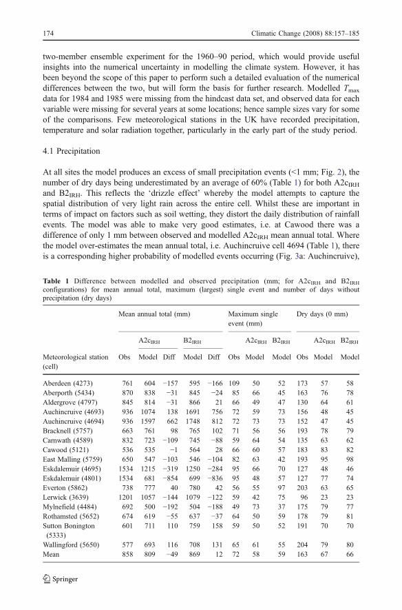
At all sites the model produces an excess of small precipitation events (<1 mm; Fig. 2), thenumber of dry days being underestimated by an average of 60% (Table 1) for both A2cIRHand B2IRH. This reflects the ‘drizzle effect’ whereby the model attempts to capture thespatial distribution of very light rain across the entire cell. Whilst these are important interms of impact on factors such as soil wetting, they distort the daily distribution of rainfallevents. The model was able to make very good estimates, i.e. at Cawood there was adifference of only 1 mm between observed and modelled A2cIRH mean annual total. Wherethe model over-estimates the mean annual total, i.e. Auchincruive cell 4694 (Table 1), thereis a corresponding higher probability of modelled events occurring (Fig. 3a: Auchincruive),

Table 1 Difference between modelled and observed precipitation (mm; for A2cIRH and B2IRHconfigurations) for mean annual total, maximum (largest) single event and number of days withoutprecipitation (dry days)

Mean annual total (mm) Maximum singleevent (mm)

Dry days (0 mm)

A2cIRH B2IRH A2cIRH B2IRH A2cIRH B2IRH

Meteorological station(cell)

Obs Model Diff Model Diff Obs Model Model Obs Model Model

Aberdeen (4273) 761 604 −157 595 −166 109 50 52 173 57 58Aberporth (5434) 870 838 −31 845 −24 85 66 45 163 76 78Aldergrove (4797) 845 814 −31 866 21 66 49 47 130 64 61Auchincruive (4693) 936 1074 138 1691 756 72 59 73 156 48 45Auchincruive (4694) 936 1597 662 1748 812 72 73 73 152 47 45Bracknell (5757) 663 761 98 765 102 71 56 56 193 78 79Carnwath (4589) 832 723 −109 745 −88 59 64 54 135 63 62Cawood (5121) 536 535 −1 564 28 66 60 57 183 83 82East Malling (5759) 650 547 −103 546 −104 82 63 42 193 95 98Eskdalemuir (4695) 1534 1215 −319 1250 −284 95 66 70 127 48 46Eskdalemuir (4801) 1534 681 −854 699 −836 95 48 57 127 77 74Everton (5862) 738 777 40 780 42 56 55 97 203 63 65Lerwick (3639) 1201 1057 −144 1079 −122 59 42 75 96 23 23Mylnefield (4484) 692 500 −192 504 −188 49 73 37 175 79 77Rothamsted (5652) 674 619 −55 637 −37 64 50 59 178 79 81Sutton Bonington(5333)

601 711 110 759 158 59 50 52 191 70 70

Wallingford (5650) 577 693 116 708 131 65 61 55 204 79 80Mean 858 809 −49 869 12 72 58 59 163 67 66

174 Climatic Change (2008) 88:157–185

Tab

le2

Differencebetweenmodelledandobserved

maxim

umtemperature

(for

A2c

IRHandB2 IRHconfigurations)formeanannu

altotal,high

estand

lowestsingleevent,andthe

numberof

days

>15

°C

Maxim

umtemperature

(°C)

Meanannual

total(°C)

Highestsing

leevent(°C)

Low

estsing

leevent(°C)

Meandays

>15

°C

Meteorologicalstation(cell)

Obs

A2 IRH

Diff

B2 IRH

Diff

Obs

A2 IRH

B2 IRH

Obs

A2 IRH

B2 IRH

Obs

A2 IRH

B2 IRH

Aberdeen(4273)

4031

3765

−266

3838

−193

2634

29−3

−6−2

8670

72Aberporth

(543

4)44

1243

62−5

043

94−1

832

2322

−51

110

682

81Aldergrov

e(479

7)44

8442

12−2

7242

54−2

3025

2432

01

−112

193

93Auchincruive(4693)

4270

4039

−231

3835

−435

2932

34−3

−8−5

107

8871

Auchincruive(4694)

4270

3787

−483

3760

−509

2931

34−3

−6−5

107

7271

Bracknell(575

7)50

2248

77−1

4549

27−9

535

4042

−7−5

−415

613

814

2Carnw

ath(4589)

4023

4029

740

8462

3035

36−1

2−3

−496

9494

Caw

ood(512

1)47

0744

72−2

3545

13−1

9434

3939

−5−4

−514

112

112

6EastMallin

g(575

9)50

9750

38−5

950

970

3541

41−6

−6−2

160

146

150

Eskdalemuir(469

5)39

1137

64−1

4738

20−9

130

3434

−10

−6−6

8576

75Eskdalemuir(480

1)39

1141

5124

042

0229

130

3539

−10

−6−5

8510

410

5Everton

(586

2)49

9849

40−5

749

97−1

3439

42−5

−7−4

151

141

145

Lerwick(363

9)33

4734

1669

3443

9722

1616

−3−1

117

10

Mylnefield(4484)

4290

4109

−181

4174

−116

2936

33−9

−3−5

112

101

103

Rothamsted

(5652)

4776

4917

141

4964

188

3441

42−7

−6−5

145

141

145

SuttonBon

ington

(533

3)47

7045

53−2

1745

86−1

8535

4042

−7−5

−614

412

512

8Wallin

gford(5650)

5047

4869

−177

4910

−137

3541

42−9

−5−3

158

137

141

Mean

4433

4312

−121

4341

−92

3134

35−6

−4−3

116

102

102

Climatic Change (2008) 88:157–185 175

Tab

le3

Differencebetweenmodelled(A

2cIRHandB2 IRHconfigurations)andobserved

minim

umtemperature

(Tmin°C

)formeanannualtotal,highestandlowestsingleevent,

andthenu

mberof

days

<0°Cand−5

°C

Minim

umtemperature

(°C)

Meanannu

altotal(°C)

Highestsing

leevent(°C)

Low

estsing

leevent(°C)

Meandays

<0(°C)

Meandays

<−5

(°C)

Meteorologicalstation(cell)

Obs

A2 IRH

Diff

B2 IRH

Diff

Obs

A2 IRH

B2 IRH

Obs

A2 IRH

B2 IRH

Obs

A2 IRH

B2 IRH

Obs

A2 IRH

B2 IRH

Aberdeen(4273)

1750

1782

3218

2878

1717

17−1

6−1

0−8

5553

457

22

Aberporth

(543

4)25

1837

111193

3748

1230

2019

19−1

0−1

−121

00

10

0Aldergrove(479

7)20

1420

6956

2127

114

1820

22−1

1−8

−744

4035

42

2Auchencruive(4693)

1964

1677

−287

1719

−245

1820

22−1

3−1

4−1

147

7263

621

13Auchencruive(4694)

1964

1644

−320

1739

−225

1819

22−1

3−1

2−1

140

7063

514

13Bracknell(575

7)19

6522

2726

222

6830

320

2626

−16

−9−9

6253

489

76

Carnw

ath(4589)

1044

1784

740

1845

801

1819

21−2

5−1

2−1

110

365

5828

98

Caw

ood(512

1)18

8819

2133

1976

8818

2324

−15

−10

−10

5362

566

76

EastMallin

g(575

9)21

8225

0832

625

5136

919

2526

−18

−8−8

4841

345

22

Eskdalemuir(469

5)12

1916

2640

716

8746

816

1921

−19

−13

−13

8972

6417

1310

Eskdalemuir(480

1)12

1915

8436

416

6344

416

2025

−19

−13

−12

8981

7317

1917

Everton

(5862)

2473

2087

−386

2150

−323

1926

28−1

1−1

5−1

237

6860

320

15Lerwick(3639)

1715

2980

1264

3008

1292

1415

15−8

−3−2

450

02

00

Mylnefield(448

4)18

1318

04−9

1856

4318

2019

−17

−9−9

5464

577

44

Rothamsted

(5652)

1925

2237

312

2277

353

1826

26−1

7−9

−10

5753

477

65

SuttonBonington

(533

3)19

6720

1144

2058

9218

2425

−16

−10

−10

5358

538

76

Wallin

gford(5650)

1904

2198

294

2239

334

1926

26−2

1−9

−10

6253

4811

76

Mean

1854

2109

254

2161

307

1821

23−1

6−1

0−9

5653

478

87

176 Climatic Change (2008) 88:157–185

with a linear increase in error up to the 25 mm size events (Fig. 3c: Auchincruive).Conversely for sites where the model under-estimates the mean annual total, i.e.Eskdalemuir cell 4801, there is a reduction in the probability of events occurring(Fig. 3a: Eskdalemuir), particularly in the range of 3–20 mm, with a linear increase inthe model-observed difference (Fig. 3c: Eskdalemuir).

For the mean annual totals, the accuracy ranges from very good (i.e. Cawood, with−1 mm and 28 mm difference for the A2cIRH and B2IRH scenarios respectively), to verypoor (i.e. Eskdalemuir cell 4801 with −854 and −836 and cell 4695 with −319 mm and−284 mm difference for the A2cIRH and B2IRH scenarios respectively). There is a generalunderestimation by the model at 10 of the 17 cells assessed (Table 1). Therefore, for siteswhere the model under-estimates the mean annual total, whilst also over-estimating thenumber of days on which precipitation events occur, the magnitude of each event(particularly in the range of about 2–30 mm) is too small. The distribution of erroneousmodelled events is biased towards those of small magnitude. Considering the proportion-ality of differences to the annual total amount, the errors occurring at the larger events aresmaller in relation to the importance of the errors for the much more frequent small to mid-range events.

The largest single observed event was at Aberdeen (109.2 mm) where the modelestimated only 50 and 52 mm (A2cIRH and B2IRH respectively). The largest single eventwas generally underestimated across all sites, with an observed mean of 72 mm comparedwith 58 and 59 mm for the A2cIRH and B2IRH configurations respectively. The largestmodelled single event was 97 mm at Everton (B2IRH), where the observed was 56 mm. Themodel’s ability to estimate the magnitude of the largest single event varied between sites,

Table 4 Comparisons of modelled (A2IRH configuration) and observed maximum (Tmax) and minimum(Tmin) air temperature for means, standard deviation and probability of equal means (P(t)) using the pairedStudent’s t test

Maximum air temperature (°C) Minimum air temperature (°C)

Mean St Dev P(t) Mean St Dev P(t)

Meteorological station (cell) A2IRH Obs A2IRH Obs A2IRH Obs A2IRH Obs

Aberdeen (4273) 10.38 11.08 4.11 4.22 0.010 4.95 4.83 3.63 4.83 0.659Aberporth (5434) 12.26 12.12 3.04 3.99 0.558 10.31 6.29 2.92 3.53 0.000Aldergrove (4797) 11.72 12.36 3.95 4.45 0.022 5.75 5.57 3.48 3.65 0.491Auchincruive (4693) 11.18 9.71 4.42 3.54 0.000 4.56 4.50 3.88 2.98 0.808Auchincruive (4694) 10.52 9.71 4.36 3.54 0.001 4.57 4.50 3.81 2.98 0.782Bracknell (5757) 13.58 13.62 5.40 5.45 0.893 6.19 5.37 4.27 3.88 0.007Carnwath (4589) 10.90 11.08 4.51 4.96 0.548 4.74 2.87 3.86 3.77 0.000Cawood (5121) 12.42 12.51 4.99 5.14 0.811 5.34 5.03 4.11 3.66 0.291East Malling (5759) 13.96 14.02 5.41 5.44 0.863 6.97 6.05 4.39 3.95 0.003Eskdalemuir (4695) 9.09 9.13 4.17 4.46 0.887 4.52 2.86 3.85 3.10 0.000Eskdalemuir (4801) 11.54 9.13 4.62 4.46 0.000 4.40 2.86 4.12 3.10 0.000Everton (5862) 13.71 13.75 5.30 4.81 0.886 5.80 6.81 4.52 3.85 0.001Lerwick (3639) 9.58 9.19 2.18 3.27 0.044 8.28 4.71 2.28 3.12 0.000Lerwick (3640) 9.45 9.19 2.81 3.27 0.215 8.25 4.71 2.35 3.12 0.000Mylnefield (4484) 11.39 11.46 4.62 4.50 0.788 5.01 4.94 3.94 3.74 0.764Rothamsted (5652) 13.68 13.15 5.49 5.55 0.136 6.21 5.32 4.33 4.00 0.004Sutton Bonington (5333) 12.69 13.12 5.09 5.19 0.201 5.59 5.43 4.13 3.80 0.607Wallingford (5650) 11.79 11.08 5.01 4.22 0.005 6.11 4.83 4.21 3.69 0.000

Climatic Change (2008) 88:157–185 177

with a general under-estimation by about 20% of the observed, with 11 of the 17 siteshaving lower maximum single events than the observed. Only at Mylnefield (A2cIRH), andEverton and Lerwick (B2IRH) did the model overestimate the largest single precipitationevent by more than 10 mm (Table 1).

The model was generally able to replicate well the patterns of mean weekly precipitation(Fig. 4), i.e. Aberporth, Rothamsted and to a lesser extent Auchincruive (cell 4693). Nosites had substantially different patterns of mean weekly precipitation.

4.2 Air temperature

The annual cycle of mean daily air temperatures shows that the difference between theRCM estimates and the observations ranges from very low, e.g. Aberdeen and Mylnefield,to high, e.g. Aberporth (Fig. 5). Overall the model tends to estimate Tmax well but tooverestimate Tmin, although this is not true of all sites. The diurnal range is too small(Fig. 6), particularly in the spring and summer. The main discrepancies in Tmax are under-estimates in the autumn and over-estimates at the beginning of the year. At Aldergrove,however, the modelled Tmin matches the observed values well, but Tmax is under estimated,except in January and February.

Both A2cIRH and B2IRH tended to overestimate the highest Tmax event at most locations,by an average of 5.5°C (excluding Aberporth and Lerwick), though at some, i.e.Aldergrove, the estimates were very close. For the lowest estimates of Tmax, the modelunder-estimates by an average of 1.5°C, but does not manage to replicate the lowerobserved Tmax values, i.e. at Carnwath (Table 2). The model underestimated the number ofdays when Tmax was >15°C by an average of 13–14 days, but by as much as 36 days(Auchincruive: cell 4694).

The highest Tmin events tend to be overestimated by an average of 4°C, but as high as9°C, i.e. Eskdalemuir and Everton. For Aberdeen both the A2cIRH and B2IRH were exactlyright (Table 3). However, for the lowest Tmin events, neither configuration managed torepresent the most extreme observed low values, being on average 6–7°C to high. FromFigs. 5 and 7, the Tmin often do not match those of the observed mean daily temperatures inthe winter period. Conversely Everton (Fig. 5), over-estimates the A2cIRH the lowest Tmin

by 2°C and generally produces Tmin data that is too low (cold) in the winter, which issurprising considering the cell contains approx. 30% sea coverage. The lowest observedTmin event of −25°C was at Carnwath, where the model only managed a −12°C estimate.The model underestimated the total number of days below 0°C in some locations andoverestimated in others. Deviations ranged from −45 (Carnwath) to +31 days (Everton). Asimilar pattern is seen in the estimates of days below −5°C, with under- and over-estimatesof −21 days (Carnwath) and +17 days (Everton).

Figure 7 uses two locations’ results to illustrate that there are locations where the modelis able to represent the temporal distribution and magnitude of highest and lowest values ofTmax and Tmin well. For Aberdeen there is a very close match between the observed andmodelled lowest values of Tmax. The model generally slightly under-estimates the highestvalues for the majority of the year, but with several larger over-estimates in early August.Also at Aberdeen, the model performs well for the highest values of Tmin throughout theyear and for the lowest values except during the winter period. At Bracknell the modelover-estimates the highest values of Tmax during the summer but under-estimates them inthe early spring, whilst there is a very good match for the lowest Tmax values (other thanduring early winter). For the highest Tmin values, the model again over-estimates in thesummer but shows a good match throughout the rest of the year. The modelled lowest Tmin

178 Climatic Change (2008) 88:157–185

values do not represent well the extreme observed lows at Bracknell and the spring andsummer values are generally overestimated. These two locations represent better examplesfrom the 17 assessed.

The match between observed and modelled mean thermal time accumulation (TTA;Fig. 8) varies considerably, i.e. Bracknell and Wallingford having only a −6 and −33°Cdaydifference in mean TTA on the last day of the year, respectively. Carnwath wasoverestimated by 257°Cday, and Auchencruive (cell 4694 – coastal) underestimatedby −480°Cday. However, data from 13 of the 17 cells showed a close match with theobserved TTA rate during the key growing season period. The largest error was at Lerwick(island location) which overestimated by 649°Cday.

The mean annual totals of Tmax and Tmin, whilst not meaningful in terms of detail ofmodel estimates, do provide a quantifiable indication of any substantial differences betweenthe modelled and observed data. Annual total Tmax is generally underestimated by a smallamount (121°C for the A2cIRH and 92°C for the B2 IRH configurations), but the total Tmin isoverestimated by an average of 254°C for A2cIRH and 307°C for B2IRH (Tables 2 and 3).

The mean annual Tmax and Tmin (Table 4), as assessed by the paired Student’s t test (P(t))confirms that the model is better able to represent Tmax than Tmin. Five locations have P(t)values exceeding 0.80 for Tmax compared with only one for Tmin. The higher P(t) values forTmax are generally found at coastal locations (i.e. Everton) or those in lowland centralEngland (i.e. Bracknell), but some nearby locations also had low P(t) values (e.g.Wallingford). Locations that had higher P(t) values for Tmax tended to have very low onesfor Tmin, with the opposite occurring when P(t) values for Tmin were high. Only Mylnefieldhad high P(t) values (>0.78) for both Tmax and Tmin.

Generally the temporal distribution of mean daily Tmax and Tmin is modelled adequately,based on the synchronisation of temporal distributions seen in Fig. 5, but with someexceptions, particularly for Aberporth and Lerwick. In both these cases the cells can beclassified as ‘sea cells’ as they contain large areas of sea. The modelled data show thecharacteristics of a sea area rather than that of land, with a small range between Tmax andTmin. As such, it is not appropriate to make direct comparisons between land basedobservation station data and modelled grid cell data where the cell contains a certainpercentage of sea. Further work is required to determine what that critical percentage of seacover is.

Locations on the boundary between two cells could show contrasting results. Forexample Eskdalemuir (cells 4695 and 4801) had similar temperature results (not shown),but a marked difference in precipitation (Table 1). Hence care has to be taken in decidingwhich cells’ data are most representative of sites on cell boundaries, i.e. through the use ofpre-defined criteria, or multiple cell analysis.

4.3 Solar radiation

The HadRM3 model systematically over-estimates So (Fig. 9). However, the model doesperform very well at some locations, such as Aberdeen and Aldergrove. At these locationsthe distribution of estimate errors is similar to that from data derived from specialistradiation models, i.e. the Donatelli–Bellocchi model (Donatelli and Bellocchi 2001;Rivington et al. 2005). The HadRM3 model estimates at these locations are in the order ofonly ±1 MJ m−2 day−1 larger than those from models like the Donatelli–Bellocchi model,but are much larger at other locations, i.e. Eskdalemuir (cell 4695) where the largest singleerror was 7.65 MJ m−2 day−1. However, specialised models such as the Donatelli–Bellocchimake both over- and under-estimates, leading to compensating errors (i.e. when used in a

Climatic Change (2008) 88:157–185 179

crop model), whereas the HadRM3 estimates are consistently overestimated. The modelover-estimates So particularly in the late summer to autumn period, when actual values arelikely to be high, but there appears to be a characteristic shift towards either accurate orunder-estimates in the spring to early summer period (i.e. Everton, Sutton Bonington,Wallingford).

4.4 Relationships between variables

The comparisons were not designed to estimate the quality of the correlation between dailyvariables, rather variables were assessed individually. However, the results produced doprovide some evidence of the models’ overall performance and relationships betweenvariables. There does not appear to be a consistent pattern whereby if the model makesgood estimates of one variable it makes equally good estimates of another. At no locationdoes the model produce high quality estimates for all variables assessed. For example, themodel estimates Tmax and Tmin very well at Mylnefield, but under-estimates precipitationand over-estimates So. Similarly at Cawood, the estimates of total annual precipitation arenearly exact with a close approximation of the largest single event, but under-estimates thenumber of dry days by 100, whilst Tmax and Tmin are estimated well (except Tmin in thesummer) but So is overestimated. At Aberdeen the model performs very well for Tmax, Tmin

and So but under-estimates the total amount of precipitation and was particularly bad forproducing too many days when precipitation occurs (Table 1).

5 Discussion

5.1 Implications for interpreting climate change projections

These results have implications for the interpretation of future projections of climate changeand impacts studies. One of the aims of this work has been to identify differences betweenRCM estimates at the grid cell scale and site-specific observed data, and as such indicatethat potential exists to correct biases. We recognise that the comparison is not a ‘like withlike’ one, but it reflects the importance of being able to provide appropriate data for site-specific climate change impacts studies. Bridging the spatial gap between grid cell scaleand specific locations within the cell in terms of data quality will present many challenges.Assessing RCM estimates of the past climate is an essential first step in order to evaluatethe utility of future projections in CCI studies. This work has highlighted that the use ofRCM data in CCI studies may only be appropriate when some form of bias correction hasbeen conducted and when the specific site is similar to the mean topographicalcharacteristics of the cell.

A fundamental issue with evaluating the quality of future projections by comparingestimates made at the grid cell scale of the past climate with site-specific observed data, isthat of knowing whether errors existing in past climate estimates are maintained (or evenpropagated) into the future projections. Given the aim of identifying bias correctionpotential between the cell and specific sites within it, then if the assumption holds true thaterrors present in the hindcast estimates will also exist in the same approximate form infuture projections, then using a standard approach of taking the differences betweenhindcast and future modelled data and applying those differences to observed data willresult in the transfer of the errors to the adjusted observed data. Hence we argue that it isbetter to identify differences between modelled hindcast and site-specific observed data,

180 Climatic Change (2008) 88:157–185

then adjust the future projections based on those differences. For example, if there is a meanover-estimation of minimum temperature of 1.5°C in the hindcast data for a particularlocation and at a certain time of year, a refined form of estimate for future projections willbe the modelled estimate minus 1.5°C. This method is independent of whether the source ofthe error is either structural (within the RCM), representational (the difference between the50 km cell and the site attributes), or RCM input data or parameterisation. However, it doesnot take account of the dynamics affecting model response to greenhouse gas forcing. Itsimply provides a means by which empirically derived correction factors can be derived.However, if the assumption is unfounded, then adjustment of future projection data basedon hindcast versus observed differences may not be appropriate.

On the basis that the assumption is correct (but not considering GHG forcing responses),when the bias based constraints of the modelled data have been identified, it becomespossible to determine where and when it is appropriate to use the future projection data insite-specific impacts studies. Based on our analysis, future projections for the RCM andscenarios tested, as currently published, of precipitation, extreme summer Tmax, mean Tmin,lowest Tmin and So are potentially unreliable at some locations. Conversely the indication isthat mean Tmax, the lowest Tmax and highest Tmin estimates are reliable. These issuesindicate that there is a need for more comparisons between RCM estimates and observeddata, to identify the characteristics of combinations of weather variables and locationswhere RCMs perform poorly and to suggest corrections that can be applied.

5.2 Precipitation

The occurrence of too many modelled small precipitation events (<0.3 mm) may not besignificant in terms of the overall soil water balance, as the amount of water added to thesurface layer is very small but sufficient to give a surface ‘wetting’ effect. However, it islikely that they will adversely affect estimates of evapotranspiration due to cooling the soilsurface and vegetation canopy temperatures. This in turn will affect soil water balances as itwill be the wetted surface water that is evaporated rather than water drawn up from lowerlevels. Estimates of pest and pathogen responses will also be distorted by the inaccuracy ofdry day estimates. The occurrence of such large numbers of small events indicates an issuewith the model’s handling of such events. One possible explanation is that errors were madeacceptable during the original model validation process, when observed data was spatiallyaggregated within a cell, giving a ‘drizzle effect’.

The fact that the model did not estimate the largest single events does not indicate afailure of the model, but that the thirty year coverage of the hindcast may not be sufficientto capture the more rare extreme events with longer return periods. In conjunction with this,the aim of the model is to represent the mean conditions for a grid cell, rather than specificextreme events recorded at individual stations. However, the consistency with which themodel underestimated the largest single event across all sites does indicate a limitation.

In order to increase the utility of the data for impact studies, we recommend a reductionin the number of days on which precipitation occurs (i.e. removing estimates less than about0.3 mm) whilst also increasing the magnitude of events >1 mm at locations where themodel is shown to underestimate mean annual totals. The ability of the model to estimatethe largest single precipitation event raises questions as to how useful the future projectiondata, in its original form, would be for use in flood risk assessment. However, the time slicefor the hindcast period is 30 years, with the possibility that this is too short in order tocapture the largest precipitation events. Therefore, the assessment should cover a longer

Climatic Change (2008) 88:157–185 181

hindcast versus observed period in order to be able to properly assess the ability of themodel to estimate the largest event.

5.3 Temperature

The net result of the models’ tendency to overestimate Tmin, whilst performing well forTmax, is that projected data will be unsuitable (location dependent) for some CCI studies, aserrors will be introduced to estimates of an entity’s temperature response, i.e. due to thermaltime accumulation, diurnal ranges, biophysical processes etc. In considering the dailyvariability of temperature, then mean values are not the best indicators of representation foraccuracy. However, the results presented here for mean daily Tmax and Tmin, their highestand lowest values, indicate that the model does perform well in producing data thatrepresents the natural temperature variability on a daily and seasonal basis. Thermal timeaccumulation (TTA) at some sites is very good, but it is possible to achieve the same ratesof accumulation but with data of very different magnitudes, i.e. different values of Tmax andTmin data can produce the same average value added to the previous day’s accumulation.Hence modelled TTA rates derived from the HadRM3 hindcast data can be similar toobserved TTA, but potentially for the wrong reasons. In some case, such as Carnwath, thedifferences between Tmax and Tmin (Fig. 6) produces substantially different rates of TTA(Fig. 8) from the observed, due to the overestimation of Tmin. This effects interpretations offuture plant and insect phenological responses due to TTA and correlations with the actualtemperature.

5.4 Solar radiation

The overestimation of So at many locations suggest that the data are unsuitable for use inimpacts studies where So is a key input. However, our personal experience has shown thatdata containing compensating errors of the type found in the So estimates from the HadRM3model (i.e. at Aldergrove, Fig. 9) can still result in reasonable derived estimations, i.e. whenused in a crop model. When the errors fluctuate between over- and under-estimates on adaily basis (i.e. Eskdalemuir cell 4659, Aldergrove, Fig. 9), the errors can cancelthemselves out in terms of their impact on crop model estimates of yield. However, thetemporal distribution of errors is critical, as over-estimation in the spring and summer willresult in too high a rate of biomass accumulation (more intercepted radiation). Thesystematic over-estimation at many sites (i.e. Rothamsted) will produce substantial errorswhen used in CCI studies. Though not assessed in this study, the over-estimation of Soindicates a flaw in the way the model represents cloud cover.

6 Conclusions

The types and magnitude of errors within the HadRM3 hindcast data presented here couldintroduce substantial errors when used within site-specific climate change impacts studies,i.e. using simulation models. Identification of errors in RCM estimates of the past climatemakes it possible to assess the utility of future projection weather variable data for impactsstudies. The hindcast data are, however, sufficiently similar to the observed data to raise thepossibility of making simple adjustments to the modelled data. On the assumption that thesame errors present in the hindcast data will also exist in the future projection data, suchadjustments could then be applied to future projections to reduce systematic errors. This

182 Climatic Change (2008) 88:157–185

will improve the reliability of the climate change data and reduce the uncertainty introducedto impact studies.

The assessment of the RCM data demonstrates the importance of evaluating the qualityof data prior to use within impact studies and for practitioners to be aware of how the datacan introduce uncertainty. The suitability of uncorrected RCM data for climate changeimpact studies depends ultimately on how and for what purpose the data are used. Thequality of the Tmax and Tmin data is sufficiently good for some locations to allow studiesusing monthly or weekly data to be made with confidence, but studies using daily datarequire caution, particularly where Tmin and extreme cold temperatures are importantfactors. Precipitation data are less reliable, particularly in respect the lowest (<0.3 mm) andhighest magnitude events and number of dry days, and are potentially unsuitable for CCimpact studies in an uncorrected form. The reliability with which additional meteorologicalmeasures can be derived depends on which data are required. There is a risk of introducingsignificant errors where derived values, e.g. soil water deficit, are estimated from severalweather variables as the potential exists for biases to occur with individual variables at thesame time. The temperature data for island locations and some coastal sites are unsuitablefor use in terrestrial impact studies (depending on the amount of sea cover within the cell).Where a location exists on the boundary between two cells, care needs to be taken indetermining which cells’ data best represents it. The choice of cell may depend on whetherprecipitation, temperature or solar radiation accuracy is more important.

This assessment of the quality of estimates made by the HadRM3 RCM for the historicalperiod of 1960–90, has primarily taken the form of graphical comparisons. Whilst moredetailed statistical assessments were possible, this exploratory analysis has yieldedsufficient detail to show that the data will have an affect on the results of climate changeimpact studies. The important message is that the type of biases identified here need to beconsidered when climate model data is used in impact studies, particularly when simulationmodels are used. The characteristics of the data and how the biases manifest themselvesmay not be obvious, therefore there is a need to appraise the suitability of the data prior touse. Further analysis is also required to characterise the correlation between weathervariables on a daily basis, to ensure that meteorological relationships are adequatelyrepresented, i.e. relationships between diurnal temperature ranges, solar radiation and cloudcover. It would also be informative to assess the behaviour of the model in terms of short-term variability, i.e. the continuation of patterns of weather from one day to the next.

Fundamentally, the results have shown that the HadRM3 RCM produces data that haveboth small and large spatially and temporally variable biases in its estimates of the past climate.Practitioners using RCM estimates for climate change impacts studies need to evaluate andquantify the biases in the data in order to determine what uncertainties they will introduce.

Acknowledgements The authors would like to thank the Scottish Executive Environmental and Rural AffairsDepartment for their funding support of this research. Thanks to Kevin Marsh at the BADC for processing theHadRM3 model data and to the Meteorological Office and Hadley Centre for permission to use their data.

References

Antic S, Laprise R, Denis B, de Elia R (2006) Testing the downscaling ability of a one-way nested regionalclimate model in regions of complex topography. Clim Dyn 26:305–325

Arnold SM, Monteith JL (1974) Plant development and mean temperature in a Teesdale habitat. J Ecol62:711–720

Climatic Change (2008) 88:157–185 183

BADC (2005) British Atmospheric Data Centre: http://badc.nerc.ac.uk/home/index.htmlBell JL, Sloan LC, Snyder MA (2004) Regional changes in extreme climatic events: a future climate

scenario. J Clim 17:81–87Creed IF, Band LE, Foster NW, Morrison IK, Nicolson JA, Semkin RS, Jeffries DS (1996) Regulation of

nitrate-N release from temperate forests: a test of the N flushing hypothesis. Water Resour Res 32:3337–3354

Donatelli M, Bellocchi G (2001) Estimates of daily global solar radiation: new developments in the softwareRadEst3.00. Proceedings of the 2nd International Symposium on Modelling Cropping Systems,Florence, Italy. 16–18 July 2001. Inst. for Biometeorology, CNR, Florence, Italy, pp 213–214

Droogers P, Aerts J (2005) Adaptation strategies to climate change and climate variability: a comparativestudy between seven contrasting river basins. Phys Chem Earth 30:339–346

Evans JP, Oglesby RJ, Lapenta WM (2005) Time series analysis of regional climate model performance. JGeophys Res Atmos 110(D4):D04104

Fowler HJ, Ekstrom M, Kilsby CG, Jones PD (2005) New estimates of future changes in extreme rainfallacross the UK using regional climate model integrations. 1. Assessment of control climate. J Hydrol300:212–233

Frei C, Christensen JH, Déqué M, Jacob D, Jones RG, Vidale PL (2002) Daily precipitation statistics inregional climate models: evaluation and intercomparison for the European Alps. J Geophys Res108:4124–4142

Holman IP, Rounsevell MDA, Shackley S, Harrison PA, Nicholls RJ, Berry PM, Audsley E (2005) Aregional, multi-sectoral and integrated assessment of the impacts of climate and socio-economic changein the UK. Clim Change 71:9–41

Hoogenboom G (2000) Contribution of agro-meteorology to the simulation of crop production and itsapplications. Agric For Meteorol 103:137–157

Hulme M, Jenkins GJ, Lu X, Turnpenny JR, Mitchell TD, Jones RG, Lowe J, Murphy JM, Hassell D,Boorman P, McDonald R, Hill S (2002) Climate change scenarios for the United Kingdom: TheUKCIP02 Scientific Report. Tyndall Centre for Climate Change Research, School of EnvironmentalSciences, University of East Anglia, Norwich, UK

Huntingford C, Jones RG, Prudhomme C, Lamb R, Gash JHC, Jones DA (2003) Regional climate-modelpredictions of extreme rainfall for a changing climate. Q J R Meteorol Soc 129:1607–1621

IPCC (2000) Inter-governmental panel on climate change, special report on emissions scenarios. CambridgeUniversity Press, UK

Jarvis CH, Baker RHA, Morgan D (2003) The impact of interpolated daily temperature data on landscape-wide predictions of invertebrate pest phenology. Agric Ecosyst Environ 94:169–181

Jenkins G, Lowe J (2003) Handling uncertainties in the UKCIP02 scenarios of climate change. HadleyCentre technical note 44, 20th November 2003. Meteorological Office, Exeter, UK

Jones CG, Willen U, Ullerstig A, Hansson U (2004) The Rossby Centre regional atmospheric climate modelpart 1: model climatology and performance for the present climate over Europe. Ambio 33:199–210

Kim J, Lee J-U (2003) A multiyear regional climate hindcast for the Western United States using themesoscale atmospheric simulation model. J Hydrometeorol 4:878–890

LADSS (2007) Land Allocation Decision Support System website. http://www.macaulay.ac.uk/LADSS/reference.shtml

Mearns LO, Giorgi F, McDaniel L, Shields C (1995) Analysis of daily precipitation in a nested regionalclimate model: comparisons with observations and doubled CO2 results. Glob Planet Change 10:55–78

Moberg A, Jones PD (2004) Regional climate model simulations of daily maximum and minimum near-surface temperatures across Europe compared with observed station data 1961–1990. Clim Dyn 23:695–715

Murphy JM, Sexton DMH, Barnett DM, Jones GS, Webb MJ, Collins M, Stainforth DA (2004)Quantification of modelling uncertainties in a large ensemble of climate change simulations. Nature430:768–772

Nijkamp P, Wang SL, Kremers H (2005) Modeling the impacts of international climate change policies in aCGE context: the use of the GTAP-E model. Econ Model 22:955–974

Nonhebel S (1994a) The effects of use of average instead of daily weather data in crop growth simulationmodels. Agric Syst 44:377–396

Nonhebel S (1994b) Inaccuracies in weather data and their effects on crop growth simulation results. I.Potential production. Clim Res 4:47–60

Peng PT, Kumar A, van den Dool H, Barnston AG (2002) An analysis of multimodel ensemble predictionsfor seasonal climate anomalies. J Geophys Res Atmos 107(D23):4710

Rivington M, Bellocchi G, Matthews KB, Buchan K (2005) Evaluation of three model estimates of solarradiation at 24 UK stations. Agric For Meteorol 132:228–243

184 Climatic Change (2008) 88:157–185

Rivington M, Matthews KB, Bellocchi G, Buchan K (2006) Evaluating uncertainty introduced to process-based simulation model estimates by alternative sources of meteorological data. Agric Syst 88:451–471

Rivington M, Matthews KB, Bellocchi G, Buchan K, Stöckle CO, Donatelli M (2007) An IntegratedAssessment approach to conduct analyses of climate change impacts on whole-farm systems. EnvironMod Software 22:202–210

Semenov MA (2002) LARS-WG: A Stochastic Weather Generator for Use in Climate Impact Studies. http://www.rothamsted.bbsrc.ac.uk/mas-models/download/LARS-WG-Manual.pdf

Soulsby C (1995) Contrasts in storm event hydrochemistry in an acidic afforested catchment in uplandWales. J Hydrol 170:159–179

Sperow M, Eve M, Paustian K (2003) Potential soil C sequestration on US agricultural soils. Clim Change57:319–339

Stöckle CO, Campbell GS, Nelson R (1999) ClimGen manual. Biological Systems Engineering Department,Washington State University, Pullman, WA. USA. http://c100.bsyse.wsu.edu/climgen/

Vidale PL, Luthi D, Frei C, Seneviratne SI, Schar C (2003) Predictability and uncertainty in a regionalclimate model. J Geophys Res 108:ACL12.1–ACL12.23

Weibull W (1961) Fatigue testing and analysis of results. Pergamon, Oxford, UKZhang XC (2005) Spatial downscaling of global climate model output for site-specific assessment of crop

production and soil erosion. Agric For Meteorol 135:215–229

Climatic Change (2008) 88:157–185 185