Evaluating Nearest-Neighbor Joinson Big Trajectory Data

Yixiang Fang, Reynold Cheng, Wenbin Tang, Silviu Maniu, Xuan Yang

Department of Computer Science, University of Hong Kong, Pokfulam Road, Hong Kong{yxfang, ckcheng, wbtang, smaniu, xyang2}@cs.hku.hk

Abstract—Trajectory data are abundant and prevalent insystems that monitor the locations of moving objects. In avehicle location-based service, the positions of vehicles are con-tinuously monitored through GPS; each vehicle is associatedwith a trajectory that describes its movement history. In speciesmonitoring, animals are attached with sensors, whose positionscan be frequently traced by scientists. An interesting avenue togenerate and discover new knowledge from these data is byquerying them. In this paper, we study the evaluation of thejoin operator on trajectory data. Given two sets of trajectorydata, M and R, our goal is to find, for each entity in M , its knearest neighbors from R.

Existing solutions for this query are designed for a singlemachine. Due to the abundance and size of trajectory data, suchsolutions are no longer adequate. We hence examine how thisquery can be evaluated in cloud environments. This problem isnot trivial, due to the complexity of the trajectory structure, aswell as the fact that both the spatial and temporal dimensionsof the data have to be handled. To facilitate this operation, wepropose a parallel solution framework using MapReduce. We alsodevelop a novel bounding technique, which enables trajectoriesto be pruned in parallel. Our approach can be used to parallelizesingle-machine-based algorithms. We further study a variant ofthe join operator, which allows query efficiency to be improved.To evaluate the efficiency and the scalability of our approaches,we have performed extensive experiments on large real andsynthetic datasets.

I. INTRODUCTION

In emerging systems that manage moving objects, a tremen-dous amount of trajectory data is often produced. In alocation-based service (LBS), for instance, the positions ofmobile phone users or vehicles are constantly captured byGPS receptors and mobile base stations [1], [2]. The locationinformation constitutes a trajectory, which depicts the move-ment of an entity in the past. In natural habitat monitoring,scientists obtain location information of wild animals byattaching sensors to them. This movement history information,or trajectory data, facilitates the understanding of the animals’behaviours [3]. Figure 1(a) illustrates six trajectories, each ofwhich is constructed by connecting three recorded locations.

Due to the increasing needs of managing trajectory data,the study of trajectory databases has recently attracted a lotof research attention [3]. One of the fundamental queriesfor this database is the join [4]–[6]. Given two sets M andR of trajectory objects, a join operator returns entity setsfrom M and R, that exhibit proximity in space and time.

O

m1

m2

m3

r1

r2

r3

k nearest neighbors

m1 r1, r2

m2 r3, r2

m3 r2, r1

m1

m2

m1

m2

m3m3

d1

d2

d3

(a) Joining two sets of trajectoriesO

m1

m2

m3

r1

r2

r3

k nearest neighbors

m1 r1, r2

m2 r3, r2

m3 r2, r1

m1

m2

m1

m2

m3m3

d1

d2

d3

(b) Join results

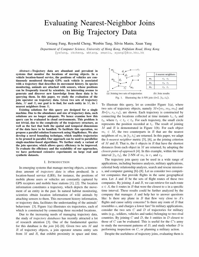
Fig. 1. Illustrating the k-NN join (k=2, [t2, t3]).

To illustrate this query, let us consider Figure 1(a), wheretwo sets of trajectory objects, namely M={m1,m2,m3} andR={r1, r2, r3}, are shown. Each trajectory is constructed byconnecting the locations collected at time instants t1, t2 andt3, where t1 < t2 < t3. For each trajectory, the small circlerepresents the position recorded at t1. The result of joiningM and R is demonstrated in Figure 1(b). For each objectmi ∈ M , the two counterparts in R that are the nearestneighbors of mi in [t2, t3] are returned. In this paper, we adaptthe k-nearest neighbor metric [5], [6], as the joining criterionof M and R. That is, the k objects in R that have the shortestdistances from each object in M are returned, by adopting theclosest-point-of-approach [4]. In this example, within the timeinterval [t2, t3], the 2-NN of m1 is r1 and r2.

The trajectory join query can be used in a wide range ofapplications, including business analysis, military applications,celestial body relationship analysis, search and rescue mission-s, and computer gaming [6]–[8]. Let us consider two competi-tor companies that provide flights in the same geographicalarea. Let A and B be the sets of flight routes of these twocompanies. By joining A and B, we can retrieve for each routea ∈ A, the k routes in B that were the closest to a in a specifictime interval. These results could be further analyzed by thecompany that manages A and help her to answer questionslike: Is there any plane in B that flew very close to A’sflights and cause safety concerns? Is there any route of B thatresembles a, and charges a lower fare? In military applications,consider the two sets C and D of trajectories for militaryunits (e.g., soldiers, vehicles and tanks) belonging to two rivalcountries. By joining C and D, the k entities in D closest tothose of C can be evaluated. This is useful for the C’s armyto study the movement patterns of D, and study whether D isperforming inspection on C, or planning a military action.

Despite the usefulness of trajectory joins, evaluating them is

not trivial. A simple solution is to evaluate a k-NN query forevery object in M . However, since a trajectory object describesthe movement of points in space and time, its data structure canbe complex and expensive to handle. The problem is worsenedwhen the sizes of the trajectory object sets to be joined arelarge. To evaluate joins on large trajectory datasets efficiently,researchers have previously studied fast algorithms and datastructures [4]–[6]. However, these approaches run trajectoryjoins on a single machine only, whose computation, memory,and disk capabilities are limited. As discussed before, extreme-ly large trajectory data have become increasingly common.Two trajectory datasets [1], [2], for instance, consist of overone billion location values. For evaluating joins on these largedata, a single machine is no longer sufficient. In this paper,we study efficient trajectory join algorithms in parallel anddistributed environments. We choose the MapReduce as theplatform for our study, since it provides decent scalability andfault tolerance for very large data processing [9].

Designing trajectory join algorithms on MapReduce is tech-nically challenging. This is because MapReduce is a shared-nothing architecture. Existing single-machine solutions oftenrely on an index (e.g., R-tree) built on top of the whole dataset(e.g., [5], [6]). As discussed in [10], [11], constructing andmaintaining an index in MapReduce can be costly. In this pa-per, we develop a solution framework that exploits the shared-nothing architecture, without using an index. We first partitionthe given trajectories of M and R into “sub-trajectories”,which are distributed to different computation units. For eachpartition of sub-trajectories, we develop a bounding techniquecalled the time-dependent bound (or TDB in short). The TDBis a time-dependent circular region containing the (candidate)objects in R, which can be the k nearest neighbors of objectsin M , in the same partition. Based on the TDB, we retrieveR’s candidates, and join them with M ’s sub-trajectories. Thejoin results of the partitions are finally merged.

Our solution can easily adopt single-machine join algo-rithms in its framework. In the paper, we will study howour approach parallelizes the execution of two single-machinesolutions. Moreover, as we will discuss, the TDB is a functionof time, and it changes according to the positions of the objectsinvolved. While computing a TDB is not straightforward, weshow that it is possible to develop a theoretically efficientalgorithm to evaluate the TDB’s in different partitions inparallel. The effort of developing TDB is justified by ourexperiments, which show that TDB significantly reduces thenumber of candidates to be examined.

We further propose two methods to optimize our joinalgorithm. First, we enhance the load balancing aspect of oursolution, by distributing the trajectory objects to computingunits in a more uniform manner. Second, we study a variantof the k-NN join, called (h, k)-NN join, which only returnsh objects in M , together with their k-NN in R, under somemonotonic aggregate function (e.g., min, max, sum or avg).As we will explain, this represents the h sets of “mostimportant” k-NNs in the join of M and R. We proposea pruning technique for (h, k)-NN join. As shown in our

experiments for real and synthetic data, our algorithm for the(h, k)-NN join is much faster than its k-NN join counterpart.

The rest of this paper is organized as follows. In SectionII, we review the related work. Section III discusses the back-ground of our solution. In Section IV we study the frameworkof our solution. In Sections V and VI, we present the detailedsolution of the k-NN join. In Section VII, we present anefficient algorithm to evaluate (h, k)-NN join. Section VIIIdiscusses the experimental results. We conclude in Section IX.

II. RELATED WORK

A substantial amount of research on nearest neighbor queryfor trajectory objects has been performed. In [5], four types ofqueries have been studied, using R-trees. Our studied query isan extension of one of these four queries, i.e., given a trajectoryobject and a time interval return the nearest neighbour duringthis time. The continuous version of nearest neighbour querieshas also received significant research attention. In [12], thenearest neighbor of every point on a line segment has beeninvestigated, while [13] studied concurrent continuous spatio-temporal queries and [8] studied the k nearest and reverse knearest neighbor queries on trajectory objects. The differencebetween our work and the above is that – for a given querytrajectory object – we wish to return k trajectory objects whosedistances to the query are minimal at some particular timeinstances, while the above studies focus on returning the knearest neighbors at every time instance.

There are also many studies on join operation for trajectoryobjects. In [4], an adaptive join algorithm is proposed forclosest-point-of-approach join, which is based on sweep linealgorithm [14]. Given two trajectory objects, their minimumdistance is defined to be achieved at their closest point. Alsoin [6] a broad class of trajectory join operations are studied,including trajectory distance join and k-NN join.

However, all these join algorithms are designed to be exe-cuted on a single machine, and hence are inefficient on largedatasets. A natural way to extend them for handling large-scaledata is to use parallel computing on a cluster of machines.There exist a few parallel computing paradigms includingMapReduce [9], Pregel, Spark and Shark [15]. Out of these,MapReduce is one of the most widely used and performs bestfor batch processing queries – such as joins – and we studyanswering k-NN join queries using the MapReduce paradigmhere. As we will discuss, the naive way to extend single-machine join algorithms for MapReduce is not scalable andefficient enough for large-scale trajectory objects due to itshigh computational cost.

Recently, many different kinds of join operations havebeen studied using MapReduce. For example, in [16] theset-similarity join is answered efficiently using MapReduce,in [11] divide-and-conquer and branch-and-bound algorithmsare developed for answering top-k similar pairs using MapRe-duce, and in [17] the multi-way theta-join query is studiedfrom a cost-effective perspective. In [18] efficient algorithmsfor k-NN join are presented using MapReduce, but they mainlyreturns approximate join results for sets of points, while our

k-NN join returns the exact result. [19] design an effectivemapping mechanism that exploits pruning rules for distancefiltering. However, since they do not deal with the temporaldimension, it is not clear how they can be applied to the dataof trajectory objects.

III. PRELIMINARIES

In this section we formally introduce the data model,problem definitions, single-machine solutions, the MapReduceframework, and a basic parallel solution using MapReduce.

A. Data Model

For ease of presentation, we consider in the followingtrajectory objects – or trajectories – in a d × d 2-D space.Note, however, that our methods can easily be applied formulti-dimensional space. Table I summarizes the symbols usedin this paper.

Definition 1: A trajectory tr of an object is a tu-ple composed of the object’s id and a list of locations(q(t1), q(t2), · · · , q(tl)). Each point q(t) is represented by atriple (x, y, t), where x and y are the positions along x and ycoordinates, and t is the timestamp of this location.

We denote the timestamps of the first and last points of tr astr.s and tr.e respectively. We assume that the trajectory objectmoves along the straight line segment q(ti)q(ti+1) betweenany two consecutive points q(ti) and q(ti+1) with constantspeed, in line with previous work [4], [6].

To evaluate k-NN queries on such trajectories, we firstdefine the associated notions of distance between trajectories.

Definition 2: The minimum distance between a point p anda line segment q(ti)q(ti+1), is defined as:

MinDist(p, q (ti) q (ti+1)

)= min

q∈q(ti)q(ti+1)|p, q|, (1)

where q is a point lying on the line segment q(ti)q(ti+1), and|p, q| is the Euclidean distance between points p and q.

Without loss of generality, our algorithm can be easilyextended for other trajectory models [3] and distance measuressuch as network distance, Manhattan distance, etc.

p

q(t1)tr tr1

tr2

q(t2)

q(t3) q(t4)

q(t')

q(t1)q(t2)q(t3)q(t4)

q(t3)q(t1)q(t2)

(a) A point and a trajectory

p

q(t1)tr tr1

tr2

q(t2)

q(t3) q(t4)

q(t5)

q(t1)q(t2)q(t3)q(t4)

q(t3)q(t1)q(t2)

(b) Two trajectories

Fig. 2. Examples of minimum and maximum distances

Definition 3: The minimum distance between a point p anda trajectory tr with l points is defined as:

MinDist(p, tr) = min16i6l−1

MinDist(p, tr.q (ti)tr.q (ti+1)

).

(2)Similarly, we can define the maximum distance MaxDist

(p, q(ti)q(ti+1)) between a point p and a line segmen-t q(ti)q(ti+1), and the maximum distance MaxDist(p, tr)between a point p and a trajectory tr.

TABLE ISUMMARY OF NOTATIONS

Notation MeaningD a d× d data spaceM(R) a set of trajectory objectsm(r) a trajectory object from M(R)

tr a trajectorytr.id the id of the trajectory object whose trajectory is trtr.q(ti) a point of tr whose time instance is titr.s, tr.e the start and end time instances of trl the total number of points in trT the number of temporal partitionsN the number of spatial partitionsH the number of trajectory groups after hashingpi the central point of i-th spatial partitionTrMi trajectories in i-th grid generated by objects from M

CRi a set of candidate trajectories from R for TrMi

GMi a group of trajectories from M whose hash values are i

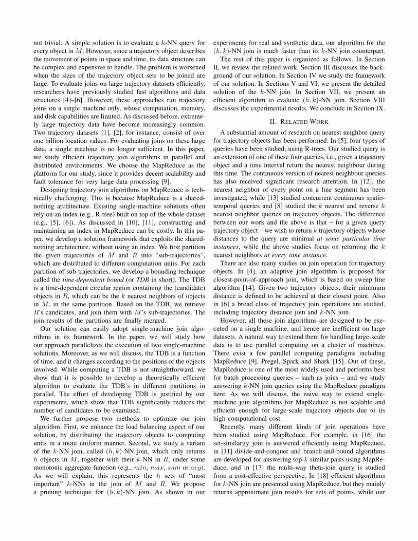
Example 1: In Figure 2(a), we can easily observe thatMinDist(p,q(t1)q(t2)) = |p, q(t′)|, MaxDist(p,q(t1)q(t2))= |p, q(t2)|, MinDist(p,tr) = |p, q(t′)| and MaxDist(p,tr)= |p, q(t4)|.

Now we have all the ingredients to define what nearestneighbour means in the context of trajectories:

Definition 4: The minimum distance between two trajecto-ries tri and trj is defined as:

MinDist(tri, trj) = mint∈∆t|tri.q(t)− trj .q(t)|, (3)

where ∆t = [tri.s, tri.e] ∩ [trj .s, trj .e].In other words, the minimum distance between two trajecto-

ry objects is the minimum distance between their trajectories.Usually, to compute the minimum distance between twotrajectory objects, we have to enumerate and compute theminimum distance between each pair of line segments fromtheir trajectories, for the time intervals which intersect. Sincewe assume that objects move along straight lines betweenconsecutive points, the distance between each pair of linesegments can be formulated as a function of time t [4], i.e.,d(t)2=at2 + bt+c, where a, b and c are parameters dependenton their velocities and initial positions. Thus their minimumdistance is the minimum value of this function during their in-tersected time interval. Similarly, we can define the maximumdistance MaxDist(tr1, tr2) between two trajectories tr1, tr2.

Example 2: In Figure 2(b), we can easily observe thatMinDist(tr1, tr2) = |tr1.q(t2), tr2.q(t2)| and MaxDist(tr1,tr2) = |tr1.q(t1), tr2.q(t1)|.

Definition 5: Given a trajectory object m and a set oftrajectory objects R, the k nearest neighbors of m are thek objects from R, whose minimum distances with m are thesmallest.

Given a trajectory object m and the k minimum distancesdm1 , · · · , dmk to its k nearest neighbors, we can define anymonotonic aggregate function f (e.g., maximum, minimum,sum or average of the k distance values [20]) on m. Withoutloss of generality, in this paper we define f(m) as the

maximum value of these k distance values:

f(m) = max1≤i≤k

dmi . (4)

B. Problem DefinitionsWe now formally define the problems studied in this paper,

i.e., k-NN and (h, k)-NN trajectory joins:Problem 1: Given sets M and R of trajectories, an integer k

and a query time interval [ts, te], the k-NN join query returnsk nearest neighbors from R for each trajectory object in Mduring the query interval.

Problem 2: Given sets M and R, two integers h, k, amonotonic aggregation function f , and a time interval [ts, te],the (h, k)-NN join query returns h objects of M , having thesmallest values of f on their k nearest neighbors.

A simple way to extend the methods in [18], [19] for ourk-NN join is to sample some points from trajectories and thenanswer the join queries on these points using these algorithmsWe call this approach Sampling-based approach. However,this increases the time complexity significantly. For example,consider two objects with their trajectories, each of whichhas l points. To compute their minimum distance the timecomplexity is O(l), since we only need to consider pairs ofline segments starting from the first points. But, if we samplel points from each of them, we need to consider l × l pairsof points and thus the time complexity is O(l2). Furthermore,the answers may be wrong. Consider an extreme case wherethe overall time intervals of M and R have no intersection.If we perform k-NN join on them, the result is null. Whileif we sample two sets of points from them respectively, andthen join them using spatial point join algorithms, we can finderroneous k nearest neighbors of each object.

C. Single-machine SolutionsWe now discuss two single-machine solutions for solving

k-NN joins, namely brute force (BF) and sweep line (SL).Brute force: This basic method simply uses nested loops

to solve the join. It first selects all the sub-trajectories ap-pearing in [ts, te]. Then it computes the minimum distancebetween each pair of trajectory objects – one from M andthe other one comes from R – and selects the k nearestneighbors for each object of M . This method is very costly,as it potentially needs to process the entire Cartesian productof the sets M and R.

Sweep line: The intuition behind this method is thefollowing: when computing the minimum distance betweentwo trajectory objects, their trajectories must overlap in sometime intervals. The sweep line method, e.g., [4], [14], sortsthe timestamps of all the points generated by objects fromR. For the trajectory of each object from M , it sweepsalong the temporal dimension and computes their minimumdistances using a dedicated data structure. As the sweep lineprogresses, the minimum distances to all the objects from Rare computed. Finally, the k nearest neighbors are selected.The main difference between BF and sweep SL is that, whentwo trajectories do not have temporal intersection, SL will notconsider them as a potential pair.

D. MapReduce Framework

MapReduce [9] is a popular paradigm for processing largedata on share-nothing distributed clusters. It consists of t-wo functions map and reduce. The map function takesa key-value pair and outputs a list of key-value pairs, i.e.,map(k1, v1)→ list(k2, v2). The reduce function takes a listof records with the same key as input and outputs a list ofkey-value pairs, i.e., reduce(k2, list(v2)) → list(k3, v3). Ina MapReduce job, when all the map functions have finished,all the intermediate results are grouped and shuffled to thereduce functions. By default, each map task processes a splitof data with the size equal to the block size of its distributedfile system, HDFS. In a MapReduce job, the number of maptasks equals to the number of splits, while number of reducetasks can be set by the users.

E. A Basic Parallel Solution Using MapReduce (BL)

We now introduce a basic parallel solution of k-NN joinusing MapReduce, i.e., BL, which has two MapReduce jobs.In the first job, it divides objects in M and R into a list ofdisjoint subsets randomly in the map(), and then joins eachpair of subsets using a single-machine solution – e.g., BF orSL – in the reduce(). Since the k nearest neighbors of anobject may be in several subsets of R, a second job wherethe k nearest neighbors are selected, from the results of thefirst MapReduce job. The main drawback of BL is its highcomputational cost, since each pair of trajectories from Mand R needs to be enumerated.

IV. SOLUTION FRAMEWORK

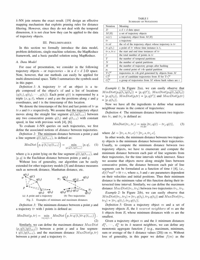
To overcome the drawback of BL, we propose a newsolution framework, which allows pruning of trajectories dur-ing the querying process. It consists of two phases, namelypreprocessing phase and query phase. The preprocessingphase needs to be conducted for only once, while the queryphase is invoked once a k-NN join query arrives. Figure 3illustrates its workflow.

In the preprocessing phase, we partition trajectories in spaceusing equal-sized grids. In the query phase, we propose a fourstage approach to answer a join query:

1) Sub-trajectory generation. In this stage, we find allthe sub-trajectories appearing in [ts, te]. Then we collectrelevant statistics from each spatial partition. We alsoselect trajectories, which serve as anchor trajectories, ifthis partition of trajectories is generated by objects fromR. We denote the set of sub-trajectories generated byobjects from M(R), in the i(j)-th grid, as TrMi (TrRj ).

2) Computing bounds. In this stage, we compute the time-dependent upper bound (TDB) of TrMi using the collect-ed statistics and the anchor trajectories.

3) Finding candidates. For each partition TrMi , we use itsTDB to find a set, CR

i , of candidate trajectories generatedby objects from R. The candidate trajectories are setsof trajectories – ideally, minimal in size – which mustcontain all the k nearest neighbors of objects in M whichcross the i-th spatial grid.

Trajectory query Computing upper bound Trajectory join

Mi MiMi

t0

f1 f2 f3

t1 t2 t3

timetr1

tr2

tr3

tr4

q1 q2 q3q' tr5

tr6

tr7

1. Sub-trajectory

generation

(Section V-A)

2. Computing

TDB

(Section V-B)

3. Finding

candidates

(Section V-C)

4.Trajectory join

(Section V-D)

Groups (G1R,…,GH

R)

Groups (G1M

,…,GHM

)

statistic and

anchor trajectories

upper bound

Preprocessing

(Section IV-B)

candidates

M, R Join result

2. Computing

TDB

(Section VI-B)

3. Finding

candidates

(Section VI-C)

4.Trajectory join

(Section VI-D)

Preprocessing

(Section V)

M, R Join result

1. Sub-trajectory

generation

(Section VI-A)

Fig. 3. The workflow of our framework

4) Trajectory join. For each partition TrMi , we join it withCR

i using a single-machine algorithm, (e.g., BF or SL).We denote the above approach as GN. Even though GN

achieves greater efficiency by using TDB, it may not ableto achieve good load balance, due to the skewness of thedistribution of the locations of the trajectory objects. By usinguniform partitioning of the space, we may encounter gridswhich contain many objects while others contain very fewobjects. To achieve good load balance in the query phase, weimprove the load balance of GN under the same framework,by using a load balance strategy, which redistributes allthe objects using some hash functions. We denote this newapproach as GL.

The preprocessing phase and each stage of the query phaseare computed using a MapReduce job, in a sequential work-flow. The purpose of the map() and reduce() for eachstage is summarized in Table II. We discuss the preprocessingin Section V. We detail the stages of GN and explain how GLimproves the load balance in Section VI.

TABLE IIDETAILS OF EACH MAPREDUCE JOB

Phase/Stage Function Main work

PreprocessingMap conduct temporal partition

Reduce conduct spatial partition

Stage 1Map generate sub-trajectories

Reduce collect statistics and anchor trajectories

Stage 2Map compute MaxDist(pi, achTr)

Reduce compute the TDB, i.e, ui(t), of TrMi

Stage 3Map find candidates of TrMi

Reduce collect the candidates of TrMi

Stage 4Map trajectory join

Reduce select k nearest neighbors for each object

V. THE PREPROCESSING PHASE

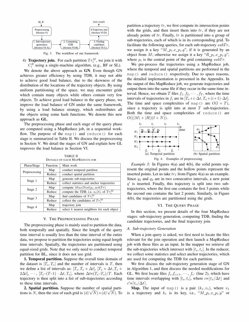
The preprocessing phase is mainly used to partition the data,both temporally and spatially. Since the length of the querytime interval is usually less than the time interval of the entiredata, we propose to partition the trajectories using equal-lengthtime intervals. Spatially, the trajectories are partitioned usingequal-sized grids. Note that we only need to conduct temporalpartition for BL, since it does not use grid.

1. Temporal partition. Suppose the overall time domain ofthe dataset is [Ts, Te] and the number of intervals is T , thenwe define a list of intervals as: [Ts, Ts + ∆t], [Ts + ∆t, Ts +2∆t], · · · , [Te–(T–1) · ∆t, Te], where ∆t=(Te–Ts)/T . Eachtrajectory is then split into a list of sub-trajectories accordingto these time intervals.

2. Spatial partition. Suppose the number of spatial parti-tions is N , then the size of each grid is (d/

√N)×(d/

√N). To

partition a trajectory tr, we first compute its intersection pointswith the grids, and then insert them into tr, if they are notalready points of tr. Finally, tr is partitioned into a group ofsub-trajectories, each of which is in its corresponding grid. Tofacilitate the following queries, for each sub-trajectory subTr,we assign it a key “M pi.x pi.y”, if it is generated by anobject from M ; otherwise we assign it a key “R pi.x pi.y”,where pi is the central point of the grid containing subTr.

We pre-process the trajectories using a MapReduce job,where the temporal and spatial partitions are performed in themap() and reduce() respectively. Due to space reasons,the detailed implementation is presented in the Appendix. Inthe output of this MapReduce job, we generate trajectories andoutput them into the same file if they occur in the same time in-terval. Hence, we obtain T files f1, f2, · · · , fT , where the timeintervals of trajectories in fi are in [Ts+i·∆t, Ts+(i+1)·∆t].The time and space complexities of map() are O(l + T ),since a trajectory is split into at most T sub-trajectories.Both the time and space complexities of reduce() areO((|M |+ |R|)(l +N)).

Trajectory query Computing upper bound Trajectory join

Mi MiMi

t0

f1 f2 f3

t1 t2 t3

timetr1

tr2

tr3

tr4

q1 q2 q3q' tr5

tr6

tr7

(a) Temporal partition

Data query Finding upper bound Join parallelly

Mi Mi

Mi

t0

f1 f2 f3

t1 t2 t3

timetr1

tr2

tr3

tr4

q1 q2 q3q' tr5

tr6

tr7

(b) Spatial partition

Fig. 4. Examples of preprocessing

Example 3: In Figures 4(a) and 4(b), the solid points rep-resent the original points and the hollow points represent theinserted points. Let us take tr1 from Figure 4(a) as an example.Since q2 and q3 are in two consecutive intervals, a new pointq′ is inserted. Finally, this trajectory is split into two sub-trajectories, where the first one contains the first 3 points whilethe second one contains the last 2 points. Similarly, in Figure4(b), the trajectories are partitioned using the grids.

VI. THE QUERY PHASE

In this section, we present details of the four MapReducestages: sub-trajectory generation, computing TDB, finding thecandidate trajectories, and the final trajectory join.

A. Sub-trajectory Generation

When a join query is asked, we first need to locate the filesrelevant for the join operation and then launch a MapReducejob with these files as an input. In the mapper we retrieve allthe sub-trajectories which intersect with [ts, te]. In the reducer,we collect some statistics and select anchor trajectories, whichare used for computing the TDB for each partition.

We first discuss the sub-trajectory generation stage of GNin Algorithm 1, and then discuss the needed modifications forGL. We first locate files fc,fc+1, · · · , fc′ (line 2), which havetime intervals overlapping with [ts, te], where c=bts/∆tc andc′=dte/∆te.

Map. The input of map() is a pair (k1, v1), where v1

is a trajectory and k1 is its key, i.e., “M pi.x pi.y” or

“R pj .x pj .y”. We extract the sub-trajectory which appearsin [ts, te] (line 4), and output it (line 5).

Reduce. We first parse the set label L, which can be eitherM or R from k2 (line 7). Then we collect some statisticinformation and anchor trajectories (line 8-11). We next detailhow the statistics and anchor trajectories are collected.

Algorithm 1 Stage 1: Sub-trajectory generation1: procedure MAP-SETUP(ts , te)2: locate files fc, fc+1, · · · , fc′ ;3: procedure MAP(k1 , v1)4: subTr ← v1.subTraj(ts, te);5: k2 ← k1; v2 ← subTr; OUTPUT(k2 , v2);6: procedure REDUCE(k2 , v2)7: parse the set label L from k2; TrLi ← v2;8: compute sT (TrLi ), eT (TrLi ), maxU(TrLi );9: if L = “R” then

10: achList← SELECTANCHOR(TrLi , sT (TrRi ), k);11: output maxU(TrLi ), sT (TrLi ), eT (TrLi ), achList, TrLi ;

In terms of statistics collected, we first collect the minimumstart time and maximum end time of all the trajectories in TrLi ,as shown in Equation (5). Moreover, for all the trajectories,we compute their maximum distances to the central point pi,and collect their maximum value, as shown in Equation (6).

sT (TrLi ) = mintr∈TrLi

tr.s, eT (TrLi ) = maxtr∈TrLi

tr.e (5)

maxU(TrLi ) = maxtr∈TrLi

MaxDist(pi, tr) (6)

To facilitate our computations, we now introduce a newdata structure, namely spatiotemporal-unit (abbreviated as st-unit). A st-unit is a triple (dist, startT , endT ), where distis a distance value, startT and endT are the start and endtime of a time interval [startT, endT ]. For each partition TrLi ,we can form a st-unit u=(maxU(TrLi ), sT (TrLi ), eT (TrLi )),where maxU(TrLi ) bounds the maximum distances from pito all the trajectories during this time interval.

In addition, if L is R, we need to collect some anchortrajectories from TrRj (line 9-10). For any time instance, ifthere are more than k trajectory objects in the grid of thispartition, then we only collect k anchor trajectories; otherwise,all of them are collected. Even though any k trajectories canbe selected as anchor trajectories, we found it is better toselect trajectories which are closest to the central points of thegrids. We propose a heuristic algorithm to select the anchortrajectories. We discuss the details in the Appendix.

Example 4: Figure 5 gives an example of computingmaxU(TrMi ) of TrMi , which contains 2 trajectories. Figure 6gives an example of 6 trajectories in TrRj (k=2). For eachtrajectory tr, we form a st-unit (MaxDist(pj , tr), tr.s, tr.e).We can observe that at any time instance, there are at least 2trajectory objects in the j-th grid. We collect the trajectorieswhich correspond to the wide lines in the figure as anchortrajectories.

GL. To balance the workload for the subsequent jobs inthe workflow, we use a hash function to redistribute all theobjects in M and R each into H disjoin groups, where H

dist

sT(TrjR) t1 t2

tr1

time

tr2

tr3

tr4

tr5

tr6

eT(TrjR)

TriM

maxU(TriM)

Fig. 5. Statistic collection

dist

sT(TrjR) t1 t2

tr1

time

tr2

tr3

tr4

tr5

tr6

eT(TrjR)

TriM

maxU(TriM)

Fig. 6. Anchor trajectory selection

can be set as the integer multiple of the maximum number ofparallel map tasks running in a cluster. The details of settingH are discussed in the Appendix In general, any hash function(e.g., [21]) which can partition objects into groups that keepthe same distribution of objects as the overall distribution canbe adopted here. In our experiments, since the identifiers oftrajectory objects in the dataset are uniformly distributed, wesimply hash the objects according to their identifiers, i.e., thehash function is a simple modulo function hash(tr)=tr.id%H .After hashing, each group has the same expected number ofobjects. We denote the trajectories of objects from M (R) inthe i(j)-th group as GM

i (GRj ).

In the sub-trajectory generation stage of GL, all the stepsare the same with Algorithm 1, except we need to redistributethe trajectories using the hash function in the reduce().Specifically, we hash each tr ∈ TrLi and assign it a key,which is a combination of its set label L and hash valuehash(tr). In the output of this MapReduce job, we outputtrajectories according to their keys, hence obtaining 2×Hfiles, corresponding to GM

1 , · · · , GMH , G

R1 , · · · , GR

H . Note thatin each file, trajectories from a same reduce() are collectedtogether and stored in a single line.

The time and space complexities of map() are O(log l) andO(l) respectively, since we can use binary search to find thesub-trajectory. The computation of sT (TrLi ), eT (TrLi ) andmaxU(TrLi ) can be performed linearly by scanning all thetrajectories. The time complexity of finding anchor trajectoriesis O(|TrLi |2l), since we need to find one from TrRj each time.Thus, the overall time and space complexities of reduce() areO(|TrLi |2l) and O(|TrLi |l) respectively.

B. Computing TDB

We first introduce the intuitions behind the time-dependentbound, which is the most important part for the efficiency ofthe algorithms. For objects whose sub-trajectories are in TrMi ,we want to compute an upper bound on the area containingall their k nearest neighbors. However, since the objects maymove arbitrarily, the area containing their k nearest neighborsmay be large in some time intervals, and small in other timeintervals. So it is nontrivial to compute a tight upper boundwhich holds in all time intervals.

Example 5: Figure 7 gives an example (k=2). The hollowpoints denote the objects from M and the solid points denotethe objects from R. Let us consider the upper bound of thecentral grid partition. At time instance t in Figure 7(a), the knearest neighbors of objects, i.e., m1 and m2, in this partitionare in a small area. But at another time instance t′ in Figure7(b), the k nearest neighbors of objects, i.e., m1 and m3, in

this partition are in a large area.

O

m1

m2

m3

r1

r2

r3

k nearest neighbors

m1 r1, r2

m2 r3, r2

m3 r2, r1

m1

m2

m1

m2

m3m3

d1

d2

d3

(a) time instance t

O

m1

m2

m3

r1

r2

r3

k nearest neighbors

m1 r1, r2

m2 r3, r2

m3 r2, r1

m1

m2

m1

m2

m3m3

d1

d2

d3

(b) time instance t′

Fig. 7. The upper bound changes with time

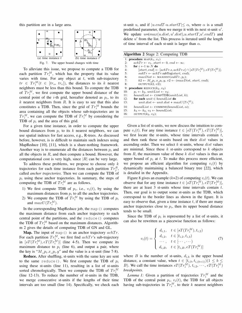
To alleviate this issue, we propose to compute a TDB foreach partition TrMi , which has the property that its valuevaries with time. For any object at t, with sub-trajectorytr ∈ TrMi (t ∈ [trs, tre]), the distances to its k nearestneighbors must be less than this bound. To compute the TDBof TrMi , we first compute the upper bound distance of thecentral point of the i-th grid, hereafter denoted as pi, to itsk nearest neighbors from R. It is easy to see that this alsoconstitutes a TDB. Then, since the grid of TrMi bounds thearea containing all the objects whose sub-trajectories are inTrMi , we can compute the TDB of TrMi by considering theTDB of pi and the area of this grid.

For a given time instance, in order to compute the upperbound distances from pi to its k nearest neighbors, we canuse spatial indexes for fast access, e.g., R-trees. As discussedbefore, however, is is difficult to maintain such indexes usingMapReduce [10], [11], which is a share-nothing framework.Another way is to enumerate all the distances between pi andall the objects in R, and then compute a bound. However, thecomputational cost is very high, since |R| can be very large.

To address these problems, we propose to choose only ktrajectories for each time instance from each partition TrRj ,called anchor trajectories. Then we can compute the TDB ofpi using these anchor trajectories. In summary, the steps ofcomputing the TDB of TrMi are as follows.

1) We first compute TDB of pi, i.e., vi(t), by using themaximum distances from pi to all the anchor trajectories.

2) We compute the TDB of TrMi by using the TDB of piand maxU(TrMi ).

In the corresponding MapReduce job, the map() computesthe maximum distance from each anchor trajectory to eachcentral point of the partitions, and the reduce() computesthe TDB of TrMi based on the maximum distances. Algorith-m 2 gives the details of computing TDB of GN and GL.

Map. The input of map() is an anchor trajectory achTr.For each partition TrMi , we first find achTr’s sub-trajectoryin [sT (TrMi ), eT (TrMi )] (line 4-5). Then we compute itsmaximum distance to pi (line 6), and output a pair, wherethe key is “M pi.x pi.y” and the value is a st-unit (line 7-8).

Reduce. After shuffling, st-units with the same key are sentto the same reduce(). We first compute the TDB of piusing these st-units (line 11), resulting in a list of st-unitssorted chronologically. Then we compute the TDB of TrMi(line 12-13). To reduce the number of st-units in the TDB,we merge consecutive st-units if the lengths of their timeintervals are too small (line 14). Specifically, we check each

st-unit u, and if |u.endT -u.startT |≤ α, where α is a smallpredefined parameter, then we merge it with its next st-unit u′.We update u=(max(u.dist, u′.dist),u.startT ,u′.endT ) anddelete u′ from the list. This process is iterated until the lengthof time interval of each st-unit is larger than α.

Algorithm 2 Stage 2: Computing TDB1: procedure MAP(k1 , v1)2: achTr ← v1, start← 0, end←∞;3: for i←1 to N do4: [start, end]← [achTr.s, achTr.e] ∩ [sT (TrMi ), eT (TrMi )];5: subTr ← achTr.subTraj(start, end);6: maxDist← MAXDIST(subTr, pi);7: k2←M pi.x pi.y, v2← (maxDist, start, end);8: OUTPUT(k2, v2);9: procedure REDUCE(k2 , v2)

10: pi ← k2, unitList← v2;11: boundList← COMPTDB(unitList, k);12: for each unit ∈ boundList do13: unit.dist← unit.dist + maxU(TrMi );14: boundList← COMBINE(boundList, α);15: k3 ← k2, v3 ← boundList;16: OUTPUT(k3 , v3);

Given a list of st-units, we now discuss the intuition to com-pute vi(t). For any time instance t ∈ [sT (TrMi ), eT (TrMi )],we first locate the st-units, whose time intervals contain t,and then rank these st-units based on their dist values inascending order. Then we select k st-units, whose dist valuesare minimal. Since these k st-units correspond to k objectsfrom R, the maximum value of these k dist values is thus anupper bound of pi at t. To make this process more efficient,we propose an efficient algorithm for computing vi(t) bydynamically maintaining a balanced binary tree [22], whichis detailed in the Appendix.

Figure 8 gives an example (k=2) of computing vi(t). We canobserve that for any time instance t ∈ [sT (TrMi ), eT (TrMi )],there are at least 3 st-units whose time intervals contain t.Then, our goal is to output some st-units as the TDB, whichcorrespond to the border lines as shown in the figure. It iseasy to observe that, given a time instance t, if there are manyanchor trajectories close to pi, then its upper bound distancetends to be small.

Since the TDB of pi is represented by a list of st-units, itcan also be rewritten as a piecewise function as follows:

vi(t) =

di,1,

di,2,

· · · ,di,B ,

t ∈ [sT (TrMi ), ti,2)

t ∈ [ti,2, ti,3)

t ∈ [· · · , · · · )t ∈ [ti,B , eT (TrMi )]

(7)

where B is the number of st-units, di,b is the upper bounddistance, a constant value, when t ∈ [ti,b, ti,(b+1))(1 ≤ b ≤B). We call the time instances sT (TrMi ), ti,2, · · · , eT (TrMi )breakpoints.

Lemma 1: Given a partition of trajectories TrMi and theTDB of the central point pi, vi(t), the TDB for all objectshaving sub-trajectories in TrMi , to their k nearest neighbors

dist

ti,1 ti,2

TriM

TrjR

maxU(TriM)

minU(TriM)

dmin

tr

upper bound

ts t1 t2 te

k = 1 ----k = 2 ----k = 3 ----

t3

sT(TriM) eT(Tri

M) time

Fig. 8. Computing vi(t)

dist

ti,1 ti,2

TriM

TrjR

maxU(TriM)

upper bound

ts t1 t2 te

k = 1 ----k = 2 ----k = 3 ----

t3

sT(TriM) eT(Tri

M) time

pi

Fig. 9. Computing ui(t)

from R at time instance t is

ui(t) = maxU(TrMi ) + vi(t), t ∈ [sT (TrMi ), eT (TrMi )].(8)

Proof: (Sketch) Figure 9 illustrates the geometric intu-ition. We compute ui(t) by linking maxU(TrMi ) with vi(t)using triangle inequality. The details are in the Appendix.

Since vi(t) is a piece-wise function, ui(t) is also a piece-wise function, whose value changes with time. We denote themaximum and minimum values of ui(t) as max(ui(t)) andmin(ui(t)) respectively.

The time and space complexities of map() are O(Nl) andO(l) respectively, since we need to enumerate all the centralpoints and anchor trajectories, which can consist of the entiretyof R in worst case. The operations on the balanced binarytree including insert, delete and query can be completed inO(log |R|) and combing st-units can be completed linearlywithout extra space cost. Thus, the time and space complexi-ties of reduce() are O(|R|log|R|) and O(|R|) respectively.

C. Finding Candidates

We now study how to find a set of candidate trajectories forjoin, CR

i , for each partition TrMi , i.e., to list all trajectorieswhich may be in the k-NN of trajectories of M crossing TrMi .Given two partitions TrRj and TrMi , we check whether thetrajectories of TrRj are the candidates of TrRi in two sequentialsteps: partition check and trajectory check.

TrxM

TrxM

TrjR

TryM

TrzM

TryM

TrzM

TrjR

maxU(TrzM

)

maxU(TryM

)+min(uy(t))

maxU(TrxM

)+max(ux(t))

maxU(TrjR)

maxU(TrzM

)+min(uz(t))

Fig. 10. Join candidate casesPartition check. Given two trajectory partitions, TrMi andTrRj , we need to check whether the whole set of trajectoriesin TrRj is the candidate of Tri, by checking three cases:

1) none of the them are join candidates of TrMi ,2) all of them are join candidates of TrMi , and3) a part of them are join candidates of TrMi .Lemma 2: Given two partitions TrMi and TrRj , if

maxU(TrMi ) +max(ui(t)) 6 |pi, pj | −maxU(TrRj ), (9)

then all the trajectories in TrRj belong to case 1, else if

maxU(TrMi ) +min(ui(t)) > |pi, pj |+maxU(TrRj ), (10)

then all trajectories in TrRj belong to case 2. Otherwise, thetrajectories belong to case 3.

Proof: (Sketch) In Figure 10, the cases between TrRj withTrMx , TrMy and TrMz are case 1, 2 and 3 respectively. We canprove each case using triangle inequality in the Appendix.

We use the above lemma to check cases 1 and 2 first. Ifnone of them holds, we need to perform individual trajectorycheck as follows.Trajectory check. To explain the trajectory check, we firstintroduce two supporting lemmas.

Lemma 3: Given a partition TrMi and a trajectory objectr ∈ R whose trajectory is tr, the lower bound distance fromr to objects which cross the partition TrMi is:

wi(tr) = max{0,MinDist(pi, tr)−maxU(TrMi )}. (11)

Proof: (Sketch) We consider the minimum distance be-tween r and an arbitrary object crossing TrMi , and then claimit is larger than wi(tr). The details are in the Appendix.

Lemma 4: Given a partition TrMi and its TDB ui(t), forany trajectory object r ∈ R, whose sub-trajectory tr appearsin [ti,b, ti,(b+1)), where ti,b and ti,(b+1) are two consecutivebreakpoints of ui(t), if the wi(tr) < ui(t), then tr is amongthe candidates of TrMi .

The lemma follows directly from the bound in Lemma 3.In the trajectory check step, we check each trajectory in

TrRj , and perform the following steps. We first collect allthe breakpoints ti,1, ti,2, · · · , ti,B of ui(t). Then, for eachtrajectory of TrRj , we split it into a list of sub-trajectoriesaccording to the breakpoints, each of which appears in onetime interval [ti,b,ti,(b+1)](1 ≤ b ≤ B). For each sub-trajectorytr, we compute its lower bound distance to objects of TrMi ,i.e., wi(tr), using Lemma 3. Finally, by using Lemma 4, wecan easily check whether it is a candidate of TrMi .

We now detail the corresponding MapReduce job of GN,and then discuss the needed modifications for GL. The detailedcorresponding pseudocode listings of GN are in the Appendix.

Map. The map() takes a partition of trajectories TrRj asinput. It enumerates each partition TrMi , and checks whichcase they belong to. If they belong to case 2, then all thetrajectories of TrRj are candidates of TrMi . Otherwise, for case3, we split each trajectory of TrRj into a list sub-trajectoriesaccording to the breakpoints of ui(t), and then check themone by one using Lemma 4.

Reduce. In the reduce(), we simply output the candi-dates of TrMi , i.e., CR

i .The output of this MapReduce job is a list of files containing

trajectories, one for each key (partition), for a total of N files.GL. Each map task handles a single group GR

j , in whicheach map() handles a subset Tr of trajectories from GR

j ,belonging to the same spatial partition. The MapReduce im-plementation principle is the same as that for GN, except theinput of map() is Tr. Since different groups have the sameexpected size, GL achieves better load balance than GN.

We denote the input of map() as Tr, i.e., TrRj or a subsetof GR

j . In the map(), we first need to enumerate all thepartitions and check the cases. If none holds, we need to

consider trajectories one by one. Thus, the overall time andspace complexities of map() are O(|Tr|Nl) and O(|Tr|l)respectively. Since we only need to output the input directly,the time and space complexities of reduce() are O(1) andO(|CR

i |l) respectively.

D. Trajectory Join

Since we have found the set, CRi , of candidates for each

partition TrMi , we join it with CRi and then output the k

nearest neighbors of each object crossing TrMi . But the resultis incomplete since an object may cross several grids. So foreach object, we need to reselect k nearest neighbors finally.

We now detail the corresponding MapReduce job of GN,and then discuss the needed modifications for GL. The detailedpseudocode listings of GN are presented in the Appendix.

Map. The input of map() is a partition TrMi . It joins TrMiwith the set CR

i of corresponding generated candidates, usinga single-machine algorithm. In this paper, we use BF or SLas discussed before, but any other single-machine trajectoryjoin algorithms can be incorporated. Finally, we output a listof pairs, where the key is the object id and the value is a listof its k nearest neighbors with their minimum distances.

Reduce. The input of reduce() is an object with itsk nearest neighbors computed from different partitions. Weoutput k objects whose minimum distances are the smallest.

GL. The principle and implementation of GL is the sameas in the finding candidates stage, i.e., each map() handles asubset of trajectories from GM

i .We denote the input of map() as Tr, i.e., TrMi or a subset

of GMi . Since we need to enumerate each pair of trajectories

without extra space cost, the time and space complexities ofmap() are O(|Tr||CR

i |l). The time and space complexitiesof reduce() are O(kN), since an object may go across atmost N grids.

VII. THE (h, k)-NN JOIN ALGORITHM

In this section, we study a variant of the k-NN join, the(h, k)-NN join and the needed adaptations to our framework.

A. Main Intuition

In the (h, k)-NN join, we wish to return h objects ofM , having the smallest values of the function f on theirtheir k nearest neighbors from R. We call these h objectstarget objects. We assume, without loss of generality that theaggregate function is max, i.e., Equation (4).

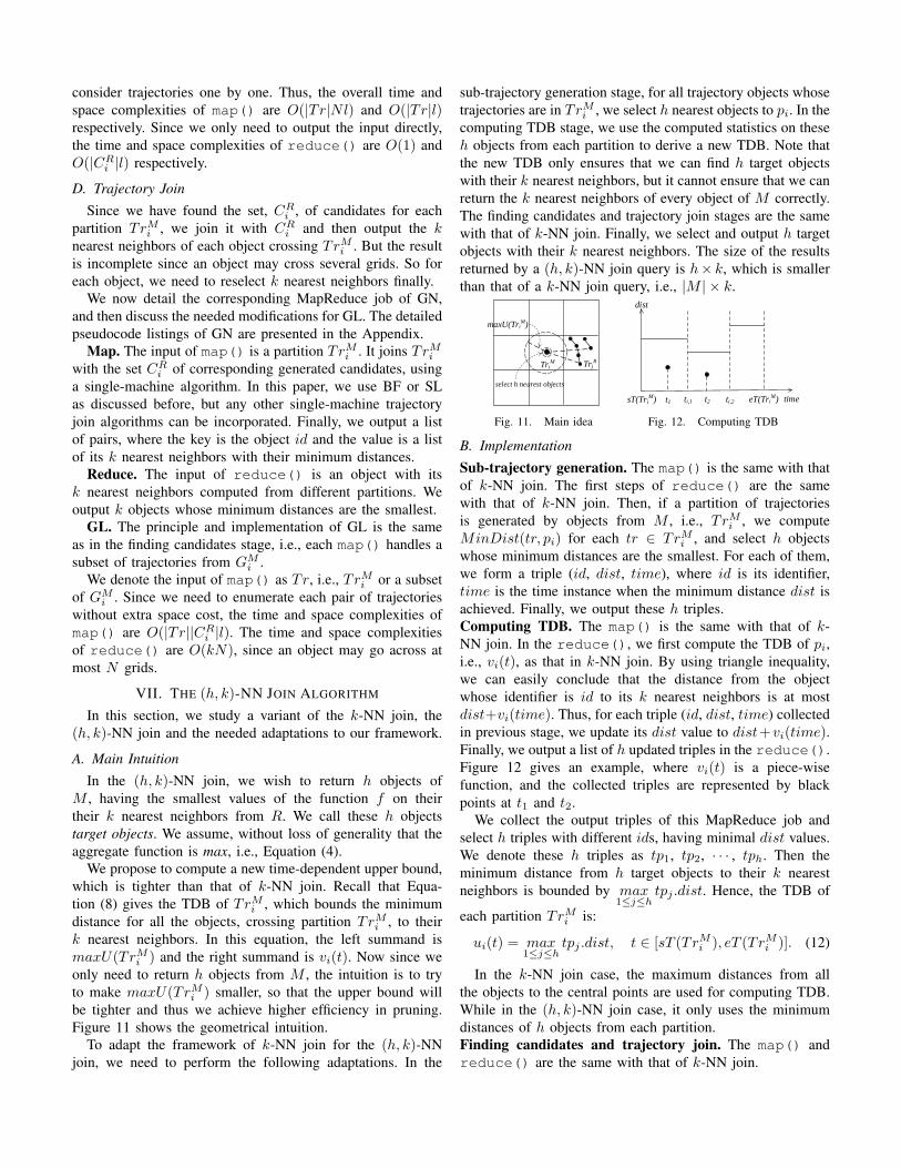
We propose to compute a new time-dependent upper bound,which is tighter than that of k-NN join. Recall that Equa-tion (8) gives the TDB of TrMi , which bounds the minimumdistance for all the objects, crossing partition TrMi , to theirk nearest neighbors. In this equation, the left summand ismaxU(TrMi ) and the right summand is vi(t). Now since weonly need to return h objects from M , the intuition is to tryto make maxU(TrMi ) smaller, so that the upper bound willbe tighter and thus we achieve higher efficiency in pruning.Figure 11 shows the geometrical intuition.

To adapt the framework of k-NN join for the (h, k)-NNjoin, we need to perform the following adaptations. In the

sub-trajectory generation stage, for all trajectory objects whosetrajectories are in TrMi , we select h nearest objects to pi. In thecomputing TDB stage, we use the computed statistics on theseh objects from each partition to derive a new TDB. Note thatthe new TDB only ensures that we can find h target objectswith their k nearest neighbors, but it cannot ensure that we canreturn the k nearest neighbors of every object of M correctly.The finding candidates and trajectory join stages are the samewith that of k-NN join. Finally, we select and output h targetobjects with their k nearest neighbors. The size of the resultsreturned by a (h, k)-NN join query is h× k, which is smallerthan that of a k-NN join query, i.e., |M | × k.

distance

TrjR

maxU(TriM)

TriM

ti,1 ti,2sT(TriM) eT(Tri

M) timet2t1

select h nearest objects

Fig. 11. Main idea

dist

TrjR

maxU(TriM)

TriM

ti,1 ti,2sT(TriM) eT(Tri

M) timet2t1

select h nearest objects

Fig. 12. Computing TDB

B. Implementation

Sub-trajectory generation. The map() is the same with thatof k-NN join. The first steps of reduce() are the samewith that of k-NN join. Then, if a partition of trajectoriesis generated by objects from M , i.e., TrMi , we computeMinDist(tr, pi) for each tr ∈ TrMi , and select h objectswhose minimum distances are the smallest. For each of them,we form a triple (id, dist, time), where id is its identifier,time is the time instance when the minimum distance dist isachieved. Finally, we output these h triples.Computing TDB. The map() is the same with that of k-NN join. In the reduce(), we first compute the TDB of pi,i.e., vi(t), as that in k-NN join. By using triangle inequality,we can easily conclude that the distance from the objectwhose identifier is id to its k nearest neighbors is at mostdist+vi(time). Thus, for each triple (id, dist, time) collectedin previous stage, we update its dist value to dist+vi(time).Finally, we output a list of h updated triples in the reduce().Figure 12 gives an example, where vi(t) is a piece-wisefunction, and the collected triples are represented by blackpoints at t1 and t2.

We collect the output triples of this MapReduce job andselect h triples with different ids, having minimal dist values.We denote these h triples as tp1, tp2, · · · , tph. Then theminimum distance from h target objects to their k nearestneighbors is bounded by max

1≤j≤htpj .dist. Hence, the TDB of

each partition TrMi is:

ui(t) = max1≤j≤h

tpj .dist, t ∈ [sT (TrMi ), eT (TrMi )]. (12)

In the k-NN join case, the maximum distances from allthe objects to the central points are used for computing TDB.While in the (h, k)-NN join case, it only uses the minimumdistances of h objects from each partition.Finding candidates and trajectory join. The map() andreduce() are the same with that of k-NN join.

Finally, for each object of M , we compute the value of theaggregate function on the distances to its k nearest neighbors.Then we output h objects – which have the h smallest valuesof the aggregate function – with their k nearest neighbors.The time and space complexities of map() and reduce()in each stage are the same with that of k-NN join.

VIII. RESULTS

We now present the experiment setting, results on k-NNjoins and (h, k)-NN joins in the following three sections.

A. Setup

Cluster: We perform experiments on a MapReduce clus-ter consisting of a master node and 60 slave nodes. Each nodehas a quad-core Intel i7-3770 3.40GHz processor, 16GB ofmemory, and 1TB of hard disk. All the nodes are connected viaGigabit Ethernet, and each node has Hadoop-2.2.0 installed.To run our experiments, we used the following Hadoop con-figuration: 1) the block size of the distributed file system is128MB, 2) the replication factor is 3, and 3) each node isconfigured to run 4 map and 4 reduce tasks. By default, weuse 60 slave nodes, and the number of reduce tasks in eachMapReduce job is set as 60× 4× 0.95=2281.

Data: We conduct our experiments on both synthetic andreal datasets. To generate the synthetic data, we use the well-known GTSD data simulator [23]. All the objects are initiallydistributed within a 104× 104 2D domain, and their positionsin x and y dimensions follow a Gaussian distribution withparameters N (5000, 40002). The average speed is 30 unitsper minute and the average time between two consecutivepoints is 1 minute. Two synthetic datasets i.e., DS1 and DS2,are generated, each of which has two sets i.e., M and R, oftrajectory objects. In DS1, each set has 104 objects and theirpositions are monitored for 25 hours in total. In DS2, eachset has 106 objects, each of which is monitored for 10 hoursin total. The total numbers of points in DS1 and DS2 are 30million and 1.2 billion respectively.

For real data, we use Beijing taxi data [1], which containsthe trajectories of 10,357 taxis in the Beijing metropolitan area.Their locations were monitored for a week by on-board GPSdevices. After throwing away points that are not in Beijingcity, it consists of 12.4 million total coordinate points. Theaverage number of points collected from each taxi is 1,260.The trajectory of each taxi is split into a list of sub-trajectories,so that time interval of each pair of consecutive points is lessthan 10 minutes. We conduct self-join on the entire dataset,i.e., the sets M and R are the same.

B. Results for k-NN Joins

We first evaluate the sampling-based approach discussed inSection III. Then, we evaluate the algorithms’ performance byvarying different parameters: N , k, tq=te–ts, i.e., the length ofquery time interval, on DS1 and Beijing taxi data. We evaluatethe effect of the number of nodes on the DS1 and Beijingdatasets. We also evaluate the scalability of the algorithms by

1http://wiki.apache.org/hadoop/HowManyMapsAndReduces/

TABLE IIIDEFAULT PARAMETER SETTINGS

Dataset Default parametersDS1 T=10, N=400, H=240, α=1 minute, k=10, tq=6 hoursDS2 T=10, N=400, H=240, α=1 minute, k=10, tq=2 hours

Beijing taxi T=10, N=400, H=240, α=3 minute, k=10, tq=1 day

varying the sizes of M and R on DS2. The default parametersettings are shown in Table III. For the purpose of reducingthe number of st-units in the TDB, we simply set the valueof α on each dataset as the average time between any twoconsecutive points. The start time ts of the query time intervalis chosen randomly. By default, we use SL as the single-machine trajectory join algorithm.

1. Sampling-based approach. We evaluate the quality ofk-NN join result returned by the sampling-based approachdiscussed in Section III. We randomly choose two subsets oftrajectories from Beijing taxi data, each of which has 1,000taxis. We join them using the sampling-based approach. Thenfor each object, we use the k nearest neighbors returned bySL as the ground truth, and compute the precision and recallof the results returned by the sampling-based approach. Ourresults show that the average precision and recall values are0.15 and 0.16 respectively. This shows that the quality of theresults returned via sampling is quite poor, mainly because thisalgorithm overlooks the temporal dimension of the trajectories.

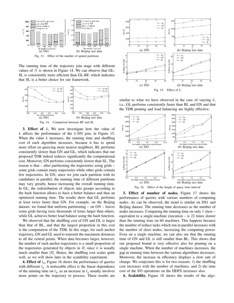
2. Effect of N . Figure 13 shows how the running timeof the algorithms is influenced by the value of N . We alsoillustrate the breakdown of the running time in each of thefour stages. When the value of N increases, the data spaceis split into more, smaller, grids. Since computing the TDBof a partition is based on the information collected from itsnearby partitions, more partitions result in a tighter TDB,which increases pruning power and increases the efficiency.But on the other hand, more partitions increase the numberof inserted points lying on the borders of grids, and henceit may create more sub-trajectories. Also, the time cost ofcomputing TDB increases as the value of N increases, sincewe need to deal with more partitions. Let us take N=1,225 inFigure 14(a) as an example. The running time of computingTDB accounts for 22% of the overall running time. The reasonis that, when N=1,225, each grid contains less than 9 objectson average, since |R|=104. All of them are selected as anchortrajectories since k=10. This demonstrates that the time costof computing TDB is very large if we use all the trajectoriesfrom R to compute the TDB, as discussed in Section IV.

Therefore, the overall time cost becomes larger when Nis either very small or very large. On balance, in our experi-ments, the overall time of these algorithms is minimized whenN=400 on each dataset. Hence, we set N=400 in subsequentexperiments. Among all the 4 stages, the trajectory join stagerunning time still takes the largest proportion of the time cost,while the sub-trajectory generation and candidate generationstage take a small proportion of the running time.

In addition, we compare the efficiency of BF and SL single-machine algorithms, when used in combination with GL. Wedenote these 2 algorithms as GL-BF and GL-SL respectively.

(a) DS1 (b) Beijing taxi data

Fig. 13. Effect of the number of spatial partitions

The running time of the trajectory join stage with differentvalues of N is shown in Figure 14. We can observe that GL-SL is consistently more efficient than GL-BF, which indicatesthat SL is a better choice for our framework.

100 225 400 625 900 12250

200

400

600

800

the number of partitions

time

(s)

GL−BFGL−SL

(a) DS1

100 225 400 625 900 12250

100

200

300

400

500

600

700

the number of partitions

time

(s)

GL−BFGL−SL

(b) Beijing taxi data

Fig. 14. Comparison between BF and SL

3. Effect of k. We now investigate how the value ofk affects the performance of the k-NN join, in Figure 15.When the value k increases, the running time and shufflingcost of each algorithm increases, because it has to spendmore effort on querying more nearest neighbors. BL performsconsistently slower than GN and GL, which indicates that ourproposed TDB indeed reduces significantly the computationalcost. Moreover, GN performs consistently slower than SL. Thereason is that – after partitioning the trajectories using grids –some grids contain many trajectories while other grids containfew trajectories. In GN, since we join each partition with itscandidates in parallel, the running time of different partitionsmay vary greatly, hence increasing the overall running time.In GL, the redistribution of objects into groups according tothe hash function allows to have a better balance and thus anoptimized running time. The results show that GL performsat least twice faster than GN. For example, on the Beijingdataset, we found that uniform partitioning – on GN – leavessome grids having taxis thousands of times larger than others,while GL achieves better load balance using the hash function.

We observed that the shuffling cost of GN and GL is largerthan that of BL, and that the largest proportion in this costis the computation of the TDB. In this stage, for each anchortrajectory, GN and GL need to transmit the maximum distancesto all the central points. When data becomes larger, however,the number of such anchor trajectories is a small proportion ofthe trajectories generated by objects in R, since k is usuallymuch smaller than |R|. Hence, the shuffling cost scales quitewell, as we will show later in the scalability experiment.

4. Effect of tq . Figure 16 shows the performance of querieswith different tq . A noticeable effect is the linear dependenceof the running time on tq , as an increase in tq usually involvesmore points on the trajectory to process. These results are

5 10 20 30 400

1000

2000

3000

4000

k

time

(s)

GLGNBL

(a) DS1

5 10 20 30 400

500

1000

1500

k

time

(s)

GLGNBL

(b) Beijing taxi data

5 10 20 30 400

2

4

6

8

k

shuf

fling

cos

t (G

B)

GLGNBL

(c) DS1

5 10 20 30 400

5

10

15

k

shuf

fling

cos

t (G

B)

GLGNBL

(d) Beijing taxi data

Fig. 15. Effect of k

similar to what we have observed in the case of varying k,i.e., GL performs consistently faster than BL and GN and thatthe TDB pruning and load balancing are highly effective.

3.0 6.0 9.0 12.0 15.00

2000

4000

6000

8000

10000

the length of query time interval (hour)

time

(s)

GLGNBL

(a) DS1

0.5 1.0 1.5 2.0 3.00

500

1000

1500

2000

2500

3000

3500

the length of query time interval (day)

time

(s)

GLGNBL

(b) Beijing taxi data

3.0 6.0 9.0 12.0 15.00

1

2

3

4

5

6

7

the length of query time interval (hour)

shuf

fling

cos

t (G

B)

GLGNBL

(c) DS1

0.5 1.0 1.5 2.0 3.00

5

10

15

the length of query time interval (day)

shuf

fling

cos

t (G

B)

GLGNBL

(d) Beijing taxi data

Fig. 16. Effect of the length of query time interval

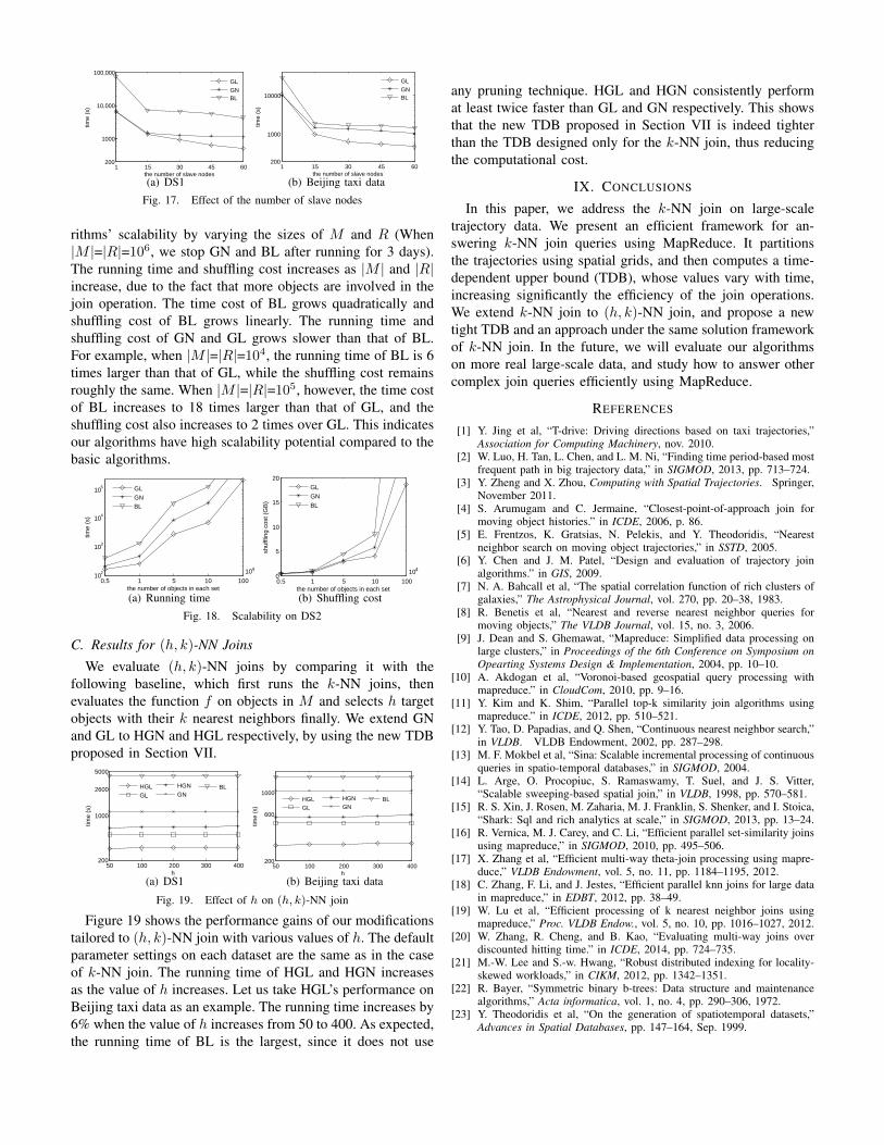
5. Effect of number of nodes. Figure 17 shows theperformance of queries with various numbers of computingnodes. As can be observed, the trend is similar on DS1 andBeijing dataset. The running time decreases as the number ofnodes increases. Comparing the running time on only 1 slave –equivalent to a single-machine execution – is 22 times slowerthan the running time on 60 machines. This happens becausethe number of reduce tasks which run in parallel increases withthe number of slave nodes, increasing the computing power.Even on a single machine, we can also see that the runningtime of GN and GL is still smaller than BL. This shows thatour proposed bound is very effective also for pruning on asingle machine. When the number of machines increases, thegap in running time between the various algorithms decreases.Moreover, the increase in efficiency displays a slow rate ofchange. We conjecture this is for two reasons: 1) the shufflingcost increases with the number of machines, and 2) the timecost of the I/O operations on the HDFS increases also.

6. Scalability. Figure 18 shows the results of the algo-

1 15 30 45 60200

1000

10,000

100,000

the number of slave nodes

time

(s)

GLGNBL

(a) DS11 15 30 45 60

200

1000

10000

the number of slave nodes

time

(s)

GLGNBL

(b) Beijing taxi data

Fig. 17. Effect of the number of slave nodes

rithms’ scalability by varying the sizes of M and R (When|M |=|R|=106, we stop GN and BL after running for 3 days).The running time and shuffling cost increases as |M | and |R|increase, due to the fact that more objects are involved in thejoin operation. The time cost of BL grows quadratically andshuffling cost of BL grows linearly. The running time andshuffling cost of GN and GL grows slower than that of BL.For example, when |M |=|R|=104, the running time of BL is 6times larger than that of GL, while the shuffling cost remainsroughly the same. When |M |=|R|=105, however, the time costof BL increases to 18 times larger than that of GL, and theshuffling cost also increases to 2 times over GL. This indicatesour algorithms have high scalability potential compared to thebasic algorithms.

0.5 1 5 10 10010

2

103

104

105

the number of objects in each set

time

(s)

GLGNBL

104

(a) Running time

0.5 1 5 10 1000

5

10

15

20

the number of objects in each set

shuf

fling

cos

t (G

B)

GLGNBL

104

(b) Shuffling cost

Fig. 18. Scalability on DS2

C. Results for (h, k)-NN Joins

We evaluate (h, k)-NN joins by comparing it with thefollowing baseline, which first runs the k-NN joins, thenevaluates the function f on objects in M and selects h targetobjects with their k nearest neighbors finally. We extend GNand GL to HGN and HGL respectively, by using the new TDBproposed in Section VII.

50 100 200 300 400200

1000

2600

5000

h

time

(s)

HGLGL

HGNGN

BL

(a) DS150 100 200 300 400

200

600

1000

h

time

(s)

HGLGL

HGNGN

BL

(b) Beijing taxi data

Fig. 19. Effect of h on (h, k)-NN join

Figure 19 shows the performance gains of our modificationstailored to (h, k)-NN join with various values of h. The defaultparameter settings on each dataset are the same as in the caseof k-NN join. The running time of HGL and HGN increasesas the value of h increases. Let us take HGL’s performance onBeijing taxi data as an example. The running time increases by6% when the value of h increases from 50 to 400. As expected,the running time of BL is the largest, since it does not use

any pruning technique. HGL and HGN consistently performat least twice faster than GL and GN respectively. This showsthat the new TDB proposed in Section VII is indeed tighterthan the TDB designed only for the k-NN join, thus reducingthe computational cost.

IX. CONCLUSIONS

In this paper, we address the k-NN join on large-scaletrajectory data. We present an efficient framework for an-swering k-NN join queries using MapReduce. It partitionsthe trajectories using spatial grids, and then computes a time-dependent upper bound (TDB), whose values vary with time,increasing significantly the efficiency of the join operations.We extend k-NN join to (h, k)-NN join, and propose a newtight TDB and an approach under the same solution frameworkof k-NN join. In the future, we will evaluate our algorithmson more real large-scale data, and study how to answer othercomplex join queries efficiently using MapReduce.

REFERENCES

[1] Y. Jing et al, “T-drive: Driving directions based on taxi trajectories,”Association for Computing Machinery, nov. 2010.

[2] W. Luo, H. Tan, L. Chen, and L. M. Ni, “Finding time period-based mostfrequent path in big trajectory data,” in SIGMOD, 2013, pp. 713–724.

[3] Y. Zheng and X. Zhou, Computing with Spatial Trajectories. Springer,November 2011.

[4] S. Arumugam and C. Jermaine, “Closest-point-of-approach join formoving object histories.” in ICDE, 2006, p. 86.

[5] E. Frentzos, K. Gratsias, N. Pelekis, and Y. Theodoridis, “Nearestneighbor search on moving object trajectories,” in SSTD, 2005.

[6] Y. Chen and J. M. Patel, “Design and evaluation of trajectory joinalgorithms.” in GIS, 2009.

[7] N. A. Bahcall et al, “The spatial correlation function of rich clusters ofgalaxies,” The Astrophysical Journal, vol. 270, pp. 20–38, 1983.

[8] R. Benetis et al, “Nearest and reverse nearest neighbor queries formoving objects,” The VLDB Journal, vol. 15, no. 3, 2006.

[9] J. Dean and S. Ghemawat, “Mapreduce: Simplified data processing onlarge clusters,” in Proceedings of the 6th Conference on Symposium onOpearting Systems Design & Implementation, 2004, pp. 10–10.

[10] A. Akdogan et al, “Voronoi-based geospatial query processing withmapreduce.” in CloudCom, 2010, pp. 9–16.

[11] Y. Kim and K. Shim, “Parallel top-k similarity join algorithms usingmapreduce.” in ICDE, 2012, pp. 510–521.

[12] Y. Tao, D. Papadias, and Q. Shen, “Continuous nearest neighbor search,”in VLDB. VLDB Endowment, 2002, pp. 287–298.

[13] M. F. Mokbel et al, “Sina: Scalable incremental processing of continuousqueries in spatio-temporal databases,” in SIGMOD, 2004.

[14] L. Arge, O. Procopiuc, S. Ramaswamy, T. Suel, and J. S. Vitter,“Scalable sweeping-based spatial join,” in VLDB, 1998, pp. 570–581.

[15] R. S. Xin, J. Rosen, M. Zaharia, M. J. Franklin, S. Shenker, and I. Stoica,“Shark: Sql and rich analytics at scale,” in SIGMOD, 2013, pp. 13–24.

[16] R. Vernica, M. J. Carey, and C. Li, “Efficient parallel set-similarity joinsusing mapreduce,” in SIGMOD, 2010, pp. 495–506.

[17] X. Zhang et al, “Efficient multi-way theta-join processing using mapre-duce,” VLDB Endowment, vol. 5, no. 11, pp. 1184–1195, 2012.

[18] C. Zhang, F. Li, and J. Jestes, “Efficient parallel knn joins for large datain mapreduce,” in EDBT, 2012, pp. 38–49.

[19] W. Lu et al, “Efficient processing of k nearest neighbor joins usingmapreduce,” Proc. VLDB Endow., vol. 5, no. 10, pp. 1016–1027, 2012.

[20] W. Zhang, R. Cheng, and B. Kao, “Evaluating multi-way joins overdiscounted hitting time.” in ICDE, 2014, pp. 724–735.

[21] M.-W. Lee and S.-w. Hwang, “Robust distributed indexing for locality-skewed workloads,” in CIKM, 2012, pp. 1342–1351.

[22] R. Bayer, “Symmetric binary b-trees: Data structure and maintenancealgorithms,” Acta informatica, vol. 1, no. 4, pp. 290–306, 1972.

[23] Y. Theodoridis et al, “On the generation of spatiotemporal datasets,”Advances in Spatial Databases, pp. 147–164, Sep. 1999.

APPENDIX

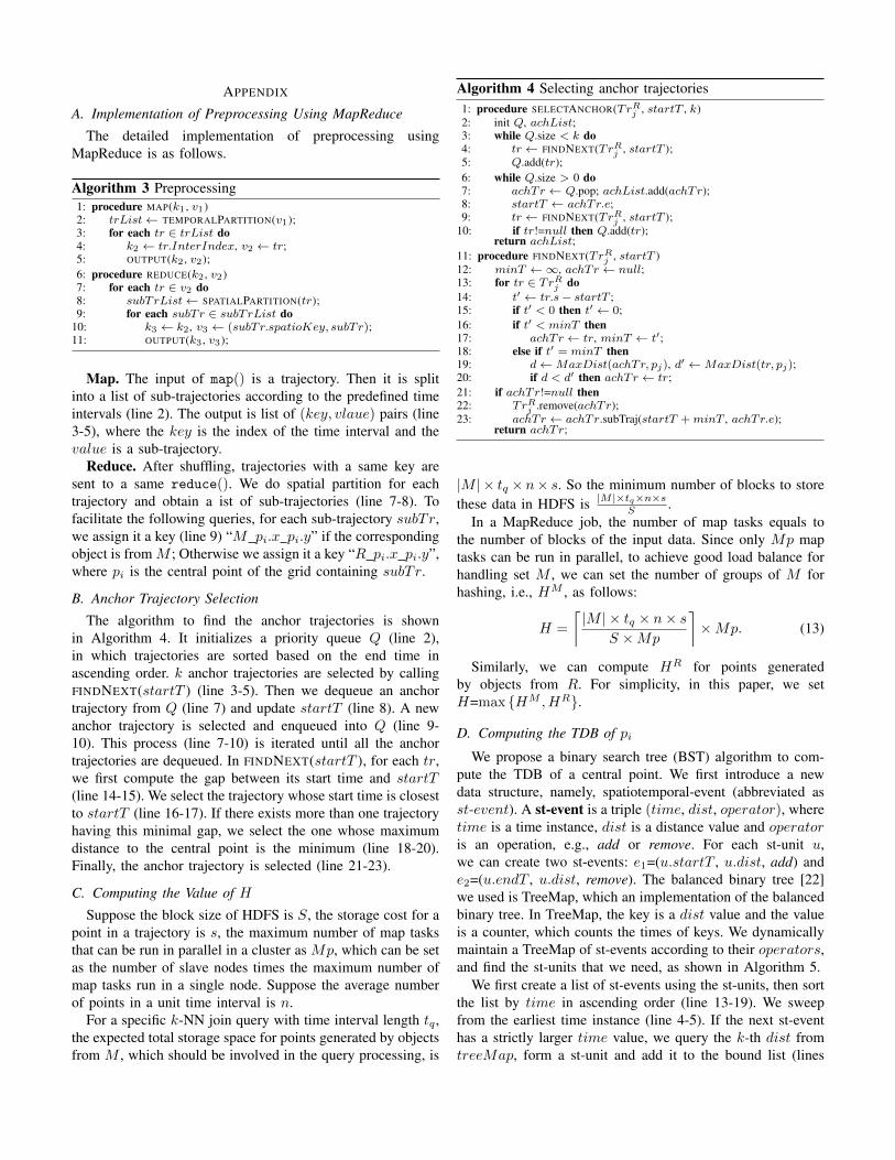
A. Implementation of Preprocessing Using MapReduce

The detailed implementation of preprocessing usingMapReduce is as follows.

Algorithm 3 Preprocessing1: procedure MAP(k1 , v1)2: trList← TEMPORALPARTITION(v1);3: for each tr ∈ trList do4: k2 ← tr.InterIndex, v2 ← tr;5: OUTPUT(k2 , v2);6: procedure REDUCE(k2 , v2)7: for each tr ∈ v2 do8: subTrList← SPATIALPARTITION(tr);9: for each subTr ∈ subTrList do

10: k3 ← k2, v3 ← (subTr.spatioKey, subTr);11: OUTPUT(k3 , v3);

Map. The input of map() is a trajectory. Then it is splitinto a list of sub-trajectories according to the predefined timeintervals (line 2). The output is list of (key, vlaue) pairs (line3-5), where the key is the index of the time interval and thevalue is a sub-trajectory.

Reduce. After shuffling, trajectories with a same key aresent to a same reduce(). We do spatial partition for eachtrajectory and obtain a ist of sub-trajectories (line 7-8). Tofacilitate the following queries, for each sub-trajectory subTr,we assign it a key (line 9) “M pi.x pi.y” if the correspondingobject is from M ; Otherwise we assign it a key “R pi.x pi.y”,where pi is the central point of the grid containing subTr.

B. Anchor Trajectory Selection

The algorithm to find the anchor trajectories is shownin Algorithm 4. It initializes a priority queue Q (line 2),in which trajectories are sorted based on the end time inascending order. k anchor trajectories are selected by callingFINDNEXT(startT ) (line 3-5). Then we dequeue an anchortrajectory from Q (line 7) and update startT (line 8). A newanchor trajectory is selected and enqueued into Q (line 9-10). This process (line 7-10) is iterated until all the anchortrajectories are dequeued. In FINDNEXT(startT ), for each tr,we first compute the gap between its start time and startT(line 14-15). We select the trajectory whose start time is closestto startT (line 16-17). If there exists more than one trajectoryhaving this minimal gap, we select the one whose maximumdistance to the central point is the minimum (line 18-20).Finally, the anchor trajectory is selected (line 21-23).

C. Computing the Value of H

Suppose the block size of HDFS is S, the storage cost for apoint in a trajectory is s, the maximum number of map tasksthat can be run in parallel in a cluster as Mp, which can be setas the number of slave nodes times the maximum number ofmap tasks run in a single node. Suppose the average numberof points in a unit time interval is n.

For a specific k-NN join query with time interval length tq ,the expected total storage space for points generated by objectsfrom M , which should be involved in the query processing, is

Algorithm 4 Selecting anchor trajectories1: procedure SELECTANCHOR(TrRj , startT , k)2: init Q, achList;3: while Q.size < k do4: tr ← FINDNEXT(TrRj , startT );5: Q.add(tr);6: while Q.size > 0 do7: achTr ← Q.pop; achList.add(achTr);8: startT ← achTr.e;9: tr ← FINDNEXT(TrRj , startT );

10: if tr!=null then Q.add(tr);return achList;

11: procedure FINDNEXT(TrRj , startT )12: minT ←∞, achTr ← null;13: for tr ∈ TrRj do14: t′ ← tr.s− startT ;15: if t′ < 0 then t′ ← 0;16: if t′ < minT then17: achTr ← tr, minT ← t′;18: else if t′ = minT then19: d←MaxDist(achTr, pj), d′ ←MaxDist(tr, pj);20: if d < d′ then achTr ← tr;21: if achTr!=null then22: TrRj .remove(achTr);23: achTr ← achTr.subTraj(startT +minT , achTr.e);

return achTr;

|M | × tq × n× s. So the minimum number of blocks to storethese data in HDFS is |M |×tq×n×sS .

In a MapReduce job, the number of map tasks equals tothe number of blocks of the input data. Since only Mp maptasks can be run in parallel, to achieve good load balance forhandling set M , we can set the number of groups of M forhashing, i.e., HM , as follows:

H =

⌈|M | × tq × n× s

S ×Mp

⌉×Mp. (13)

Similarly, we can compute HR for points generatedby objects from R. For simplicity, in this paper, we setH=max {HM , HR}.

D. Computing the TDB of piWe propose a binary search tree (BST) algorithm to com-

pute the TDB of a central point. We first introduce a newdata structure, namely, spatiotemporal-event (abbreviated asst-event). A st-event is a triple (time, dist, operator), wheretime is a time instance, dist is a distance value and operatoris an operation, e.g., add or remove. For each st-unit u,we can create two st-events: e1=(u.startT , u.dist, add) ande2=(u.endT , u.dist, remove). The balanced binary tree [22]we used is TreeMap, which an implementation of the balancedbinary tree. In TreeMap, the key is a dist value and the valueis a counter, which counts the times of keys. We dynamicallymaintain a TreeMap of st-events according to their operators,and find the st-units that we need, as shown in Algorithm 5.

We first create a list of st-events using the st-units, then sortthe list by time in ascending order (line 13-19). We sweepfrom the earliest time instance (line 4-5). If the next st-eventhas a strictly larger time value, we query the k-th dist fromtreeMap, form a st-unit and add it to the bound list (lines

6-9). Then, we continue updating the treeMap using the st-events according to their operators (lines 10-11). Finally, weobtain a list of sorted st-units, i.e., vi(t).

Algorithm 5 Computing the TDB of the central point1: procedure COMPTDB(stunitList, k)2: treeMap← INITTREEMAP<DIST, COUNTER>;3: eventList← CREATESTEVENT(stunitList);4: startT ← eventList[0].time; TDB ← INITLIST;5: for each event ∈ eventList do6: if event.time > startT then7: kthDist← treeMap.FINDKTH(k);8: TDB.addStUnit(startT , event.time, kthDist);9: startT ← event.time;

10: if event.operator=“add” then treeMap[event.dist] += 1;11: else treeMap[event.dist] -= 1;12: return TDB;13: procedure CREATESTEVENT(stunitList)14: eventList← null;15: for each unit ∈ stunitList do16: eventList.addEvent(unit.startT , unit.dist, “add”);17: eventList.addEvent(unit.endT , unit.dist, “remove”);18: SORTBYTIME(eventList);19: return eventList;

E. Proof of Lemma 1

Proof: Figure 9 illustrates the geometric intuition ofthe lemma. Consider an arbitrary time instance t ∈[st(TrMi ), et(TrMi )). Suppose the k nearest neighbors of piare rj(1 6 j 6 k) ∈ R. Then |pi, rj | 6 vi(t).

Now let us consider an arbitrary object m at t, whose sub-trajectory subTr is in TrMi . By using triangle inequality, thedistance from m to rj is

|m, rj | 6 |m, pi|+ |pi, rj | (14)

Since |m, pi| 6MaxDist(pi, subTr) 6 maxU(TrMi ), wehave

|m, rj | 6 maxU(TrMi ) + vi(t) (15)

The above equation implies that the distances from mto these k objects are bounded by maxU(TrMi ) + vi(t).Hence, for all objects having sub-trajectories in TrMi at t,the upper bound distance to its k nearest neighbors from R isui(t)=maxU(TrMi ) + vi(t).

F. Proof of Lemma 2

Proof: Consider two arbitrary trajectories, one from TrMiand one from TrRj . Then consider two points pMi and pRj onthe two trajectories, occurring at the same time instance. Usingtriangle inequality, we have:

|pMi , pRj | > |pi, pRj | − |pi, pMi |> |pi, pj | − |pj , pRj | − |pi, pMi |> |pi, pj | −maxU(TrRj )−maxU(TrMi )

(16)

|pMi , pRj | 6 |pi, pRj |+ |pi, pMi |6 |pi, pj |+ |pj , pRj |+ |pi, pMi |6 |pi, pj |+maxU(TrRj ) +maxU(TrMi )

(17)

If their minimum distance is larger than max(ui(t)), thennone of the trajectories in TrRj are candidates. If their max-imum distance is larger than min(ui(t)), then all of thetrajectories in TrRj are candidates. For other cases, a part ofthem are the candidates. Hence, Lemma 2 holds.

G. Proof of Lemma 3

Proof: Consider an arbitrary object m whose sub-trajectory is in TrMi , and the time instance tmin ∈ [tr.s, tr.e)when the minimum distance between m and r occurs. Denotem and r’s positions at tmin as pmi and prj respectively. Usingthe triangle inequality, we have:

|pmi , prj | > |pi, prj | − |pi, pmi |>MinDist(pi, tr)−maxU(TrMi )

(18)

For other time instance t ∈ [trs, tre], their distance must belarger than |pmi , prj |. Also, we know that |pmi , prj | > 0. Hence,the lower bound distance from r to objects whose trajectoriesare in TrMi is max{0,MinDist(pi, tr)−maxU(TrMi )}.

H. Implementation of Finding Candidates Using MapReduce

Algorithm 6 gives the detailed implementation of thisMapReduce job in GN.

Map. The map() takes a partition of trajectories TrRj asinput. It enumerates each partition TrMi , and checks whichcase they belong to (line 3-4). If they belong to case 2, thenall the trajectories of TrRj are candidates of TrMi (line 6-8).Otherwise, for case 3, we split each trajectory of TrRj into alist sub-trajectories according to the breakpoints of ui(t), andthen check them one by one using Lemma 4 (line 9-14).

Reduce. In the reduce(), we simply output the candi-dates of TrMi , i.e., CR

i .

Algorithm 6 Stage 3: Finding candidates1: procedure MAP(k1 , v1)2: TrRj ← v1;3: for i←1 to N do4: case← CHECK(pi , ui(t), maxU(TrMi ), maxU(TrRj ));5: k2 ← pi.x pi.y;6: if case=2 then //Partition check7: for tr ∈ Tr do8: v2 ← tr; OUTPUT(k2 , v2);9: else if case=3 then //Trajectory check

10: for tr ∈ Tr do11: subTrList← SPLIT(tr, ui(t));12: for subTr ∈ subTrList do13: if subTr is a candidate then //Use Lemma 414: v2 ← tr; OUTPUT(k2 , v2);15: procedure REDUCE(k2 , v2)16: OUTPUT(k2 , v2);

I. Implementation of Trajectory Join Using MapReduce

Algorithm 7 gives the detailed implementation of thisMapReduce job in GN.

Map. The input of map() is a partition TrMi (line 2).It joins TrMi with the set CR

i of corresponding generatedcandidates, using a single-machine algorithm (line 3-4). In thispaper, we use BF or SL as discussed before, but any other

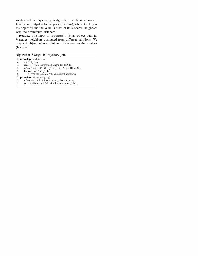
single-machine trajectory join algorithms can be incorporated.Finally, we output a list of pairs (line 5-6), where the key isthe object id and the value is a list of its k nearest neighborswith their minimum distances.

Reduce. The input of reduce() is an object with itsk nearest neighbors computed from different partitions. Weoutput k objects whose minimum distances are the smallest(line 8-9).

Algorithm 7 Stage 4: Trajectory join1: procedure MAP(k1 , v1)2: TrMi ← v1;3: read CR

i from Distributed Cache (or HDFS);4: kNNList← JOIN(TrMi , CR

i , k); // Use BF or SL5: for each tr ∈ TrMi do6: OUTPUT(tr.id, kNN ); //k nearest neighbors7: procedure REDUCE(k2 , v2)8: kNN ← reselect k nearest neighbors from v2;9: OUTPUT(tr.id, kNN ); //final k nearest neighbors