Evaluating Environmental Impact of Traffic Congestion in Real Time Based on Sparse Mobile Crowd-sourced Data

February 2018

A Research Report from the National Center for Sustainable Transportation

Peng Hao, University of California, Riverside

Chao Wang, University of California, Riverside

About the National Center for Sustainable Transportation

The National Center for Sustainable Transportation is a consortium of leading universities committed to advancing an environmentally sustainable transportation system through cutting-edge research, direct policy engagement, and education of our future leaders. Consortium members include: University of California, Davis; University of California, Riverside; University of Southern California; California State University, Long Beach; Georgia Institute of Technology; and University of Vermont. More information can be found at: ncst.ucdavis.edu.

Disclaimer

The contents of this report reflect the views of the authors, who are responsible for the facts and the accuracy of the information presented herein. This document is disseminated under the sponsorship of the United States Department of Transportation’s University Transportation Centers program, in the interest of information exchange. The U.S. Government and the State of California assumes no liability for the contents or use thereof. Nor does the content necessarily reflect the official views or policies of the U.S. Government and the State of California. This report does not constitute a standard, specification, or regulation. This report does not constitute an endorsement by the California Department of Transportation (Caltrans) of any product described herein.

Acknowledgments

This study was funded by a grant from the National Center for Sustainable Transportation (NCST), supported by USDOT and Caltrans through the University Transportation Centers program. The authors would like to thank the NCST, USDOT, and Caltrans for their support of university-based research in transportation, and especially for the funding provided in support of this project.

The authors would also like to thank Jill Luo, Xiaonian Shan, Kanok Boriboonsomsin, Guoyuan Wu and Matthew Barth for their valuable input and feedback throughout the project. Special thanks go to Lee Provost from Caltrans for providing guidance throughout this project. Thanks also go to the technical advisory board for this project.

Evaluating Environmental Impact of Traffic Congestion in Real Time Based on Sparse

Mobile Crowd-sourced Data A National Center for Sustainable Transportation Research Report

February 2018

Peng Hao, Center for Environmental Research and Technology (CE-CERT), University of California, Riverside

Chao Wang, Center for Environmental Research and Technology (CE-CERT), University of California, Riverside

[page left intentionally blank]

i

TABLE OF CONTENTS

EXECUTIVE SUMMARY .................................................................................................................... iii

1. Introduction ................................................................................................................................ 1

1.1 Background ........................................................................................................................... 1

1.2 Project Scope ........................................................................................................................ 2

1.3 Methodology Overview ........................................................................................................ 3

2. Traffic Condition Estimation ....................................................................................................... 5

2.1 Problem Statement ............................................................................................................... 5

2.2 Modal Activity Based Vehicle Dynamic Model for Freeways ............................................... 7

2.3 Model Calibration ............................................................................................................... 10

2.4 Numerical Experiments ....................................................................................................... 13

3. Emission and Dispersion Estimation for Freeways ................................................................... 18

3.1 Emission Estimation using Mobile and PeMS data ............................................................. 18

3.2 Freeway Air Pollutant Visualization in ArcMap .................................................................. 21

4. Emission and Dispersion Estimation for Arterials ..................................................................... 23

4.1 Emission Estimation for Arterials ........................................................................................ 23

4.2 Dispersion Estimation for Arterials ..................................................................................... 26

5. Air Pollution Visualization for Los Angeles ............................................................................... 30

5.1 Summary of the Estimation and Visualization Method ...................................................... 30

5.2 Visualizing Air Pollution Level of Los Angeles ..................................................................... 32

6. Conclusions ............................................................................................................................... 40

7. References ................................................................................................................................ 41

Appendix I: Acronyms and Abbreviations ..................................................................................... 43

Appendix II: Glossary .................................................................................................................... 44

Appendix III: Publication ............................................................................................................... 45

ii

List of Figures

Figure 1. Quality Assurance Air Monitoring Sites in Los Angeles, CA ............................................. 2

Figure 2. System Architecture ......................................................................................................... 4

Figure 3. Vehicle driving modes assumption on different types of road ....................................... 6

Figure 4. Problem formulation of vehicle trajectory reconstruction ............................................. 7

Figure 5. Modal transition assumption ........................................................................................... 8

Figure 6. Observed frequency of the values of = v̂ v ........................................................... 11

Figure 7. Result of a vehicle trajectory estimation ....................................................................... 13

Figure 8. Results of vehicle location-time trajectory estimation.................................................. 14

Figure 9. The coverage of mobile data in Los Angeles, CA ........................................................... 15

Figure 10. Average link speed in downtown LA ............................................................................ 17

Figure 11. Speed trajectory of a probe vehicle and speeds at vehicle detection stations at SR-91....................................................................................................................................................... 19

Figure 12. Study area and PeMS station locations in downtown, Los Angeles ............................ 20

Figure 13. PM 2.5 emissions per freeway link under PM peak traffic in August 2013 ................. 21

Figure 14. PM 2.5 concentration in downtown LA for PM peak traffic in August 2013 ............... 22

Figure 15. Intersections with manual/automatic traffic counts in downtown, LA ...................... 24

Figure 16. PM 2.5 emissions per link under PM peak traffic in August 2013 ............................... 25

Figure 17. PM 2.5 concentration under PM peak traffic in August 2013 ................................. 26

Figure 18. Daily Mean PM2.5 Concentration for Los Angeles-North Main Street Station ........... 27

Figure 19. CO concentration under PM peak traffic in August 2013............................................ 28

Figure 20. NOx concentration under PM peak traffic in August 2013 ......................................... 29

Figure 21. Layer properties settings in ArcMap ............................................................................ 31

Figure 22. PM2.5 concentration comparison between CalEnviroScreen and proposed method 33

Figure 23. Annual peak hour PM2.5 emissions in Los Angeles ..................................................... 34

Figure 24. Annual peak hour PM2.5 concentration in Los Angeles .............................................. 35

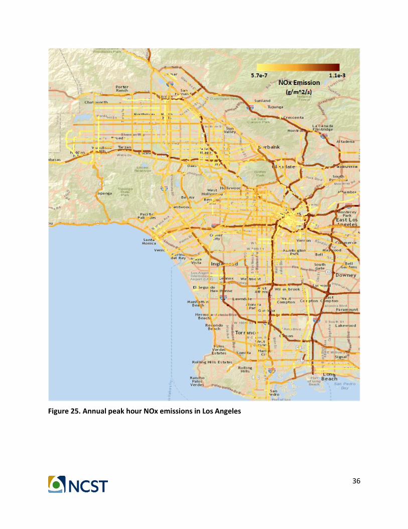
Figure 25. Annual peak hour NOx emissions in Los Angeles ........................................................ 36

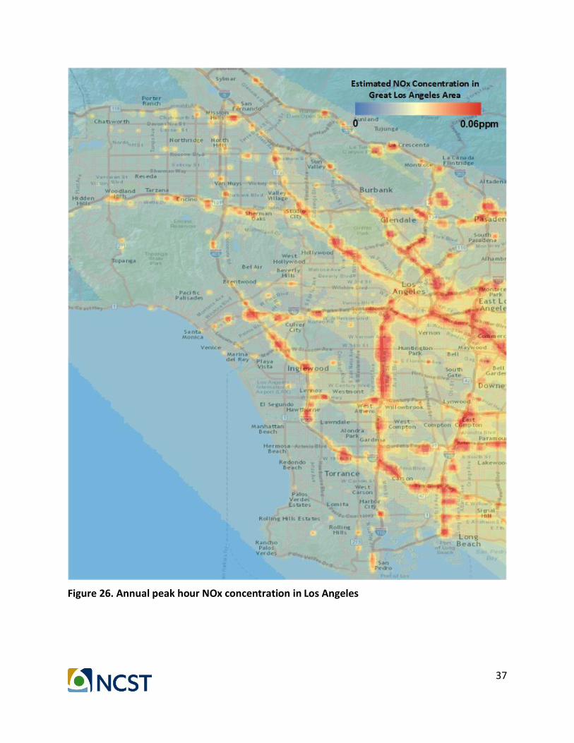
Figure 26. Annual peak hour NOx concentration in Los Angeles ................................................. 37

Figure 27. Annual peak hour CO2 emissions in Los Angeles ........................................................ 38

Figure 28. Annual peak hour CO2 concentration in Los Angeles ................................................. 39

iii

Evaluating Environmental Impact of Traffic Congestion in Real Time Based on Sparse Mobile Crowd-sourced Data

EXECUTIVE SUMMARY

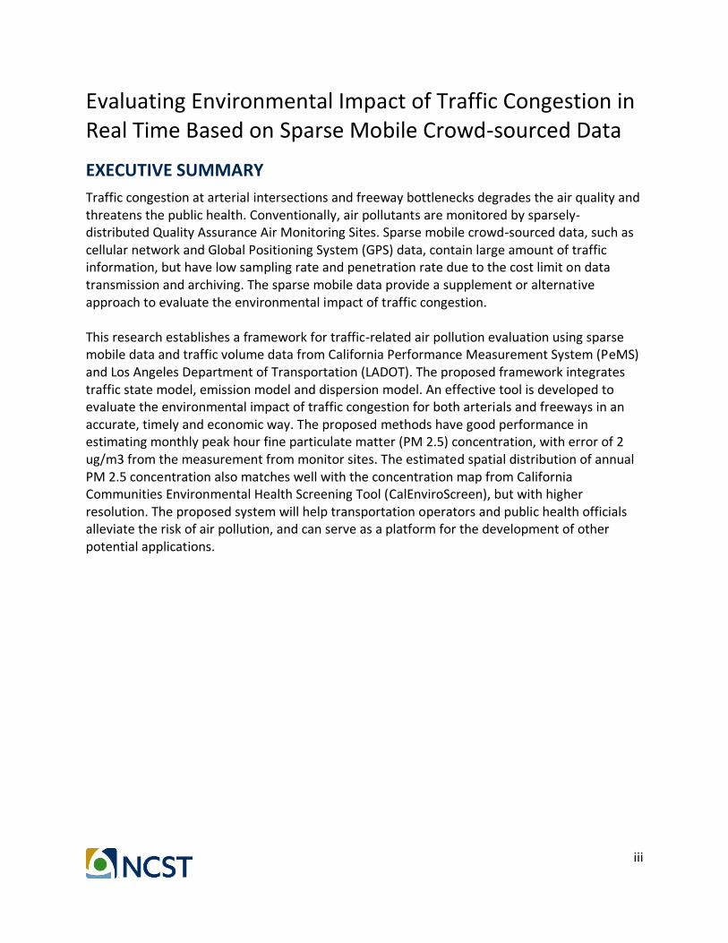
Traffic congestion at arterial intersections and freeway bottlenecks degrades the air quality and threatens the public health. Conventionally, air pollutants are monitored by sparsely-distributed Quality Assurance Air Monitoring Sites. Sparse mobile crowd-sourced data, such as cellular network and Global Positioning System (GPS) data, contain large amount of traffic information, but have low sampling rate and penetration rate due to the cost limit on data transmission and archiving. The sparse mobile data provide a supplement or alternative approach to evaluate the environmental impact of traffic congestion. This research establishes a framework for traffic-related air pollution evaluation using sparse mobile data and traffic volume data from California Performance Measurement System (PeMS) and Los Angeles Department of Transportation (LADOT). The proposed framework integrates traffic state model, emission model and dispersion model. An effective tool is developed to evaluate the environmental impact of traffic congestion for both arterials and freeways in an accurate, timely and economic way. The proposed methods have good performance in estimating monthly peak hour fine particulate matter (PM 2.5) concentration, with error of 2 ug/m3 from the measurement from monitor sites. The estimated spatial distribution of annual PM 2.5 concentration also matches well with the concentration map from California Communities Environmental Health Screening Tool (CalEnviroScreen), but with higher resolution. The proposed system will help transportation operators and public health officials alleviate the risk of air pollution, and can serve as a platform for the development of other potential applications.

1

1. Introduction

1.1 Background

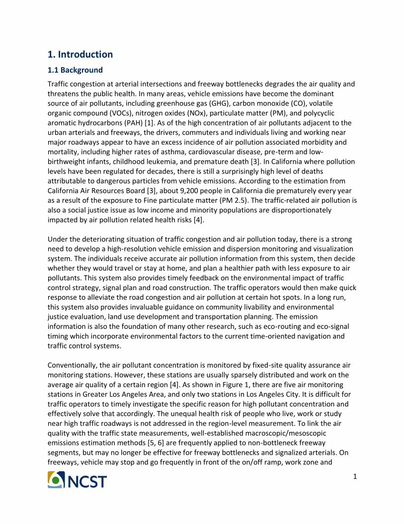
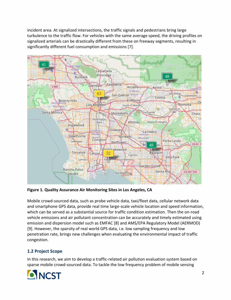
Traffic congestion at arterial intersections and freeway bottlenecks degrades the air quality and threatens the public health. In many areas, vehicle emissions have become the dominant source of air pollutants, including greenhouse gas (GHG), carbon monoxide (CO), volatile organic compound (VOCs), nitrogen oxides (NOx), particulate matter (PM), and polycyclic aromatic hydrocarbons (PAH) [1]. As of the high concentration of air pollutants adjacent to the urban arterials and freeways, the drivers, commuters and individuals living and working near major roadways appear to have an excess incidence of air pollution associated morbidity and mortality, including higher rates of asthma, cardiovascular disease, pre-term and low-birthweight infants, childhood leukemia, and premature death [3]. In California where pollution levels have been regulated for decades, there is still a surprisingly high level of deaths attributable to dangerous particles from vehicle emissions. According to the estimation from California Air Resources Board [3], about 9,200 people in California die prematurely every year as a result of the exposure to Fine particulate matter (PM 2.5). The traffic-related air pollution is also a social justice issue as low income and minority populations are disproportionately impacted by air pollution related health risks [4]. Under the deteriorating situation of traffic congestion and air pollution today, there is a strong need to develop a high-resolution vehicle emission and dispersion monitoring and visualization system. The individuals receive accurate air pollution information from this system, then decide whether they would travel or stay at home, and plan a healthier path with less exposure to air pollutants. This system also provides timely feedback on the environmental impact of traffic control strategy, signal plan and road construction. The traffic operators would then make quick response to alleviate the road congestion and air pollution at certain hot spots. In a long run, this system also provides invaluable guidance on community livability and environmental justice evaluation, land use development and transportation planning. The emission information is also the foundation of many other research, such as eco-routing and eco-signal timing which incorporate environmental factors to the current time-oriented navigation and traffic control systems. Conventionally, the air pollutant concentration is monitored by fixed-site quality assurance air monitoring stations. However, these stations are usually sparsely distributed and work on the average air quality of a certain region [4]. As shown in Figure 1, there are five air monitoring stations in Greater Los Angeles Area, and only two stations in Los Angeles City. It is difficult for traffic operators to timely investigate the specific reason for high pollutant concentration and effectively solve that accordingly. The unequal health risk of people who live, work or study near high traffic roadways is not addressed in the region-level measurement. To link the air quality with the traffic state measurements, well-established macroscopic/mesoscopic emissions estimation methods [5, 6] are frequently applied to non-bottleneck freeway segments, but may no longer be effective for freeway bottlenecks and signalized arterials. On freeways, vehicle may stop and go frequently in front of the on/off ramp, work zone and

2

incident area. At signalized intersections, the traffic signals and pedestrians bring large turbulence to the traffic flow. For vehicles with the same average speed, the driving profiles on signalized arterials can be drastically different from these on freeway segments, resulting in significantly different fuel consumption and emissions [7].

Figure 1. Quality Assurance Air Monitoring Sites in Los Angeles, CA Mobile crowd-sourced data, such as probe vehicle data, taxi/fleet data, cellular network data and smartphone GPS data, provide real time large-scale vehicle location and speed information, which can be served as a substantial source for traffic condition estimation. Then the on-road vehicle emissions and air pollutant concentration can be accurately and timely estimated using emission and dispersion model such as EMFAC [8] and AMS/EPA Regulatory Model (AERMOD) [9]. However, the sparsity of real world GPS data, i.e. low sampling frequency and low penetration rate, brings new challenges when evaluating the environmental impact of traffic congestion.

1.2 Project Scope

In this research, we aim to develop a traffic-related air pollution evaluation system based on sparse mobile crowd-sourced data. To tackle the low frequency problem of mobile sensing

3

data, the previously developed stochastic arterial trajectory estimation model is extended to freeways. Unique features of freeway driving modal activity is considered. For the low penetration problem at freeways traffic, we incorporate the sparse mobile sensing data to the California Performance Measurement System (PeMS). The PeMS data provide reliable real time traffic volume count and truck ratio under free flow condition. At freeway bottlenecks, the mobile sensing probe will better help track the stop-and-go behavior and estimate accurate average speed. For urban arterials, traffic count data from Los Angeles Department of Transportation (LADOT) also provide intersection-based traffic volume information to support the emission and dispersion estimation. The expected contribution of the proposed research is summarized as follows:

1) This research will establish a framework for vehicle emission and dispersion estimation using both sparse mobile sensing data and existing traffic volume data. The proposed framework integrates traffic state model, emission model (e.g., EMFAC) and dispersion model (e.g., AERMOD).

2) The proposed model is applicable to varying traffic conditions and multiple transport modes on either urban arterials or freeways, and adaptable to multiple mobile and fixed- location data source.

3) The proposed emission and dispersion system will provide suggestions to the transportation operator and public health officials to alleviate the risk of air pollutant. It could serve as an essential supplement of sparsely-distributed Quality Assurance Air Monitoring Stations.

4) This research will provide a platform for other applications, such as eco-routing application which help reduce the driver and pedestrian’s exposure to air pollution, and connected vehicle based eco-signal timing.

1.3 Methodology Overview

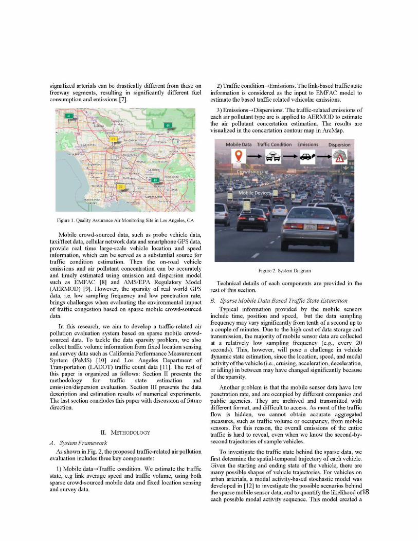
As shown in Figure 2, the proposed traffic-related air pollution evaluation includes three key components:

1) Mobile data→Traffic condition. We estimate the traffic state, e.g., link average speed and traffic volume, using both sparse crowd-sourced mobile data and fixed location sensing and survey data.

2) Traffic condition→Emissions. The link-based traffic state information is considered as the input to EMFAC model to estimate the based traffic related vehicular emissions.

3) Emissions→Dispersions. The traffic-related emissions of each air pollutant type are applied to AERMOD to estimate the air pollutant concertation estimation. The results are visualized in the concertation contour map in ArcMap.

4

Figure 2. System Architecture Typical information provided by the mobile sensors include time, position and speed, but the data sampling frequency may vary significantly from tenth of a second up to a couple of minutes. Due to the high cost of data storage and transmission, most mobile sensor data are collected at a relatively low sampling frequency (e.g., every 20 seconds). This, however, will pose a challenge in vehicle dynamic state estimation, since the location, speed, and modal activity of the vehicle (i.e., cruising, acceleration, deceleration, or idling) in between may have changed significantly because of the sparsity. Another problem is that the mobile sensor data have low penetration rate, and may be collected by different companies and public agencies. They are archived and transmitted with different format, and difficult to access. As most of the traffic flow is hidden, we cannot obtain accurate aggregated measures, such as traffic volume or occupancy, from mobile sensors. For this reason, the overall emissions of the entire traffic are hard to reveal, even when we know the second-by-second trajectories of sample vehicles. To tackle this problem, we also collect traffic volume information from fixed location sensing and survey data such as California Performance Measurement System (PeMS) [10] and Los Angeles Department of Transportation (LADOT) traffic count data [11].

5

The traffic state information for certain time intervals are applied to EMFAC model to estimate vehicular emissions. For freeways, traffic volume and truck ratio records collected from PeMS are also incorporated to the model to solve the data sparsity issue. For arterials, the traffic volume information is acquired from either historical manual count or flow estimation methods. In AERMOD, we estimate the short-range dispersion of air pollutant emissions. The pollutant emission and dispersion are visualized in ArcMap. The rest of this report is organized as follows: Section 2 presents the methodology and numerical validation for traffic state estimation method. Section 3 and 4 present the emission/dispersion estimation methods and results for freeways and arterials respectively. Section 5 applies the proposed method to the City of Los Angeles and visualizes the air pollution in ArcMap. The last section summarizes this report with discussion of future direction.

2. Traffic Condition Estimation

2.1 Problem Statement

For mobile crowd-sourced data, the sample rate is usually 10s – 60s, so only 1% - 6% of each entire speed/acceleration rate profile is revealed. It is a challenge to accurately estimate arterial link average speed based on sparse mobile sensor data. If a vehicle passes two or more links between a pair of Global Positioning System (GPS) data points, it is difficult to distribute the travel time into each link as the speed is varying during this process. The proposed vehicle trajectory estimation method can solve this problem by finding an optimal vehicle trajectory under an optimal modal activity sequence. The link average speed can then be calculated based on the trajectory segments on each link. To investigate the traffic state behind the sparse data, we first determine the spatial-temporal trajectory of each vehicle. Given the starting and ending state of the vehicle, there are many possible shapes of vehicle trajectories. For vehicles on urban arterials, a modal activity-based stochastic model was developed in [12] to investigate the possible scenarios behind the sparse mobile sensor data, and to quantify the likelihood of each possible modal activity sequence. This model created a sampling pool of all possible vehicle dynamic states. A detailed vehicle trajectory can be reconstructed using the optimal modal activity sequence which maximizes the likelihood.

6

Idling Acceleration Cruising

Acceleration

Deceleration

Cruising

Idling

Idling Acceleration Cruising Deceleration Idling

(a) Vehicle activity assumption on arterial road

(b) Vehicle activity assumption on freeway

Source: [13]

Figure 3. Vehicle driving modes assumption on different types of road The arterial model proposed in [12] adopted modal activity sequence assumption that the driving modes of a vehicle must evolve with a certain pattern, i.e. idling (1) → acceleration (2) → cruise (3)→ deceleration (4) →idling (1) →…periodically in Figure 3(a). It is reasonable when a vehicle is traveling on an arterial road with frequent stop-and-go maneuver at traffic signals and during congestions. For the freeway traffic, the vehicles may stop frequently in a short period at the bottleneck, and may travel at low speed after a significant deceleration [13]. As shown in Figure 3(b), the vehicle may keep its speed for a while within the acceleration or deceleration process (i.e., acceleration→ cruising → acceleration or deceleration → cruising → deceleration). Under heavy traffic, the driver may control the speed to avoid stop-and-go maneuver. The vehicle may decelerate early, cruise at low speed and then accelerate to catch up leading vehicles. In general, the vehicle may cruise at any speed below speed limit, including zero if we regard idling mode as a special cruising condition. Based on the relaxed assumption for freeways, we identify the type, time and distance of each modal activity based on the location and speed information of a GPS pair with certain sampling rate. Two major issues are discussed in this section: 1) identification of inflection speed point which is defined as the inflection point in the trajectory between an acceleration and a deceleration process or vice versa; and 2) determination of modal travel time and distance.

7

Time (seconds)

Spee

d (

m/s

)

u2

u1

Part Ⅰ Part Ⅱ

AccelerationDeceleration Cruising

v̂

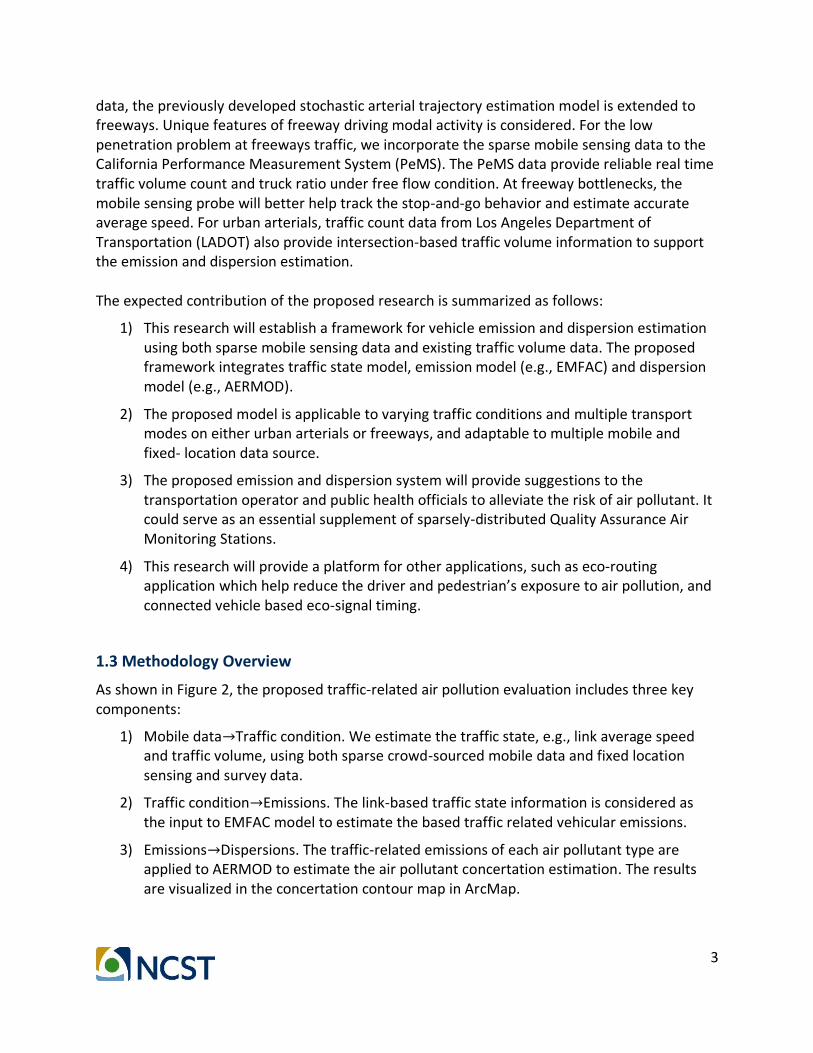
Figure 4. Problem formulation of vehicle trajectory reconstruction As shown in Figure 4, for a certain GPS data pair, the starting speed (u1), ending speed (u2), time interval ( t ) and total traveling distance ( d ) are given. The key objective in trajectory estimation is to identify modal activity sequence and assign appropriate travel time and distance to each mode. We assume that there is at most one inflection speed point ( v̂ ) between a data pair based on observations. The value of the inflection speed point should be identified before estimating times and distances that the vehicle takes under acceleration and deceleration modes. The remaining time and distance are distributed to one or multiple cruising mode segment. The crucial challenge is to estimate the time and distance for each cruising segment and assign them to the adequate position of the vehicle trajectory.

2.2 Modal Activity Based Vehicle Dynamic Model for Freeways

For a modal activity based trajectory estimation problem, the vehicle dynamic state is an essential bridge between sparse GPS data and estimated second-by-second trajectories, as it includes all key information for trajectory reconstruction. For an arterial problem, the vehicle dynamic state is determined by the modal activity sequence (i.e., M), free flow speed (i.e., U), along with the travel time (denoted as Ti) and distance (denoted as Xi) of each mode. The free flow speed is important for the arterial case as it is always considered as the average speed of cruising mode, the starting speed of deceleration mode, ending speed of the acceleration mode. For the freeway scenario, as the mode transition may happen at any speed below the speed limit, we relax that assumption. A modal transition speed vector V is introduced to substitute U. The first element of V is the starting speed (u1) of the GPS data pair, and the last one is the ending speed (u2). The elements in between are the speeds at all modal transition sequentially. Apparently, V has one more element than M.

8

As shown in Figure 5, the assumption on mode activity sequence is also relaxed for freeway cases. Some sequences, such as deceleration → cruising → acceleration, are allowed in the freeway model. However, we ignore some sequences that are statistically trivial in real world to simplify the model because of the extremely low probability of occurrence, such as acceleration → cruising → acceleration or deceleration → cruising → deceleration. For example, statistics on NGSM US101 dataset [14] shows that if the sampling time interval is 10s, almost all cruising processes occurs at the start / end of a time interval, or between acceleration and deceleration modes at the inflection speed point. The percentage of an intermediate cruising process within the process of acceleration (i.e. acceleration → cruising → acceleration) is 2.7%. For deceleration, the percentage is only 0.6%. Based on that assumption, modal transition only happens at the starting speed, ending speed and inflection speed with ten seconds time interval, as shown in Figure 5. Values of the three elements in the modal transition speed V can only be u1, v̂ and u2.

Time

Sp

eed

CruisingCruisingCruising Deceleration Acceleration

Time interval

u2

u1

Distance

v̂

v

Figure 5. Modal transition assumption For a given vehicle trajectory, there exists a certain vehicle dynamic state {m, v, t, x}. For the example case in Figure 5, M = [3,4,3,2,3]T and V = [u1,u1, v̂ , v̂ ,u2,u2]T. T and X are the time and distance for the five modal activities in M respectively. Similar as the arterial model in [12], we assume a truncated normal distribution for the acceleration/deceleration pace (i.e., the reciprocal of the average acceleration rate). We also assume the distance under acceleration/deceleration mode follows another truncated normal distribution factored by the modal travel time and speed. For the cruising or idling mode, the modal travel time and distance are assumed to be uniformly distributed. Note that in this study idling is regarded as a special cruising driving mode. Furthermore, to a certain driving mode, travel time and distance could be equal to zero.

9

The vehicle dynamic state (M) is dependent on the relationship among u1, u2 and v (average speed /v d t ). Note that if the vehicle only experiences a single acceleration or deceleration process in a certain time interval, the average speed must fall between the starting and ending speed. Therefore, if the value of v is not between u1 and u2, i.e.

max 1 2max( , )v u u u or min 1 2min( , )v u u u , there must be an inflection speed point. On the

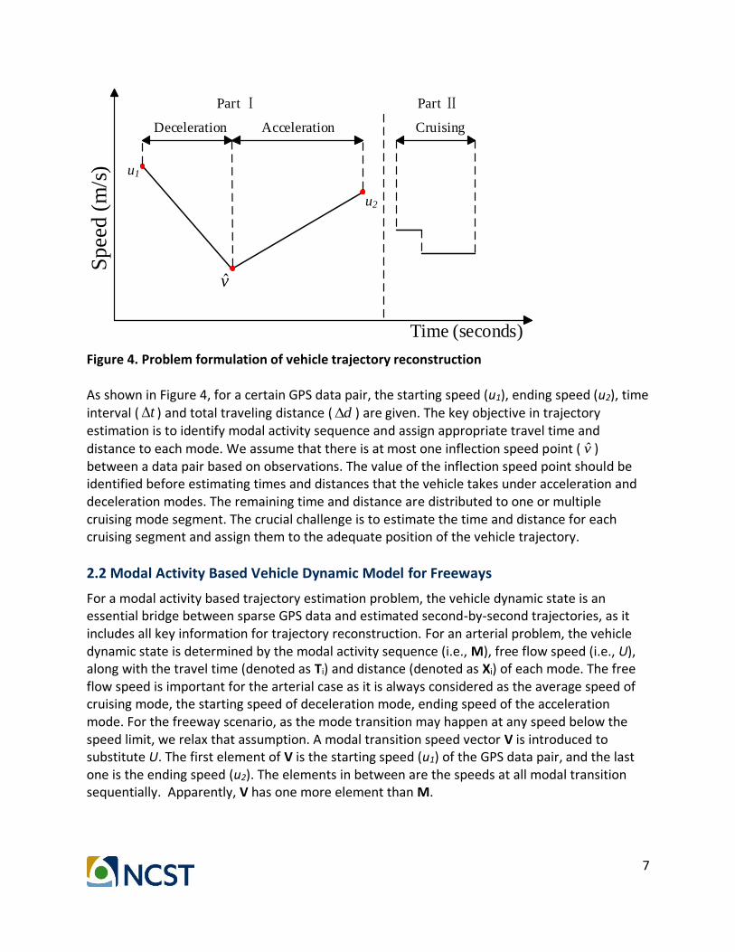
contrary, if the value of v is between u1 and u2, the existence of the inflection speed point is undefined. In this research we simply assume that the probability of M is equally distributed when there is no extreme speed point. Obviously, if there is an extreme speed, the length of M (M=[mi1]m×1) is 5; and the length of M is 3 when there is no extreme speed. Probabilities of M are shown in Table 1. Table 1. Probability of different modal activity sequence

P(M=m) maxv u minv u min max[ , ]v u u

M = [3,4,3,2,3]T 0 1 0.25

M = [3,2,3,4,3]T 1 0 0.25

M = [3,2,3]T 0 0 0.25

M = [3,4,3]T 0 0 0.25

After determining vehicle dynamic states (m), the lengths of v, t and x could be also determined. Then probability of V could be calculated using (1). The prior probability of the extreme speed v̂ will be explored in the next subsection.

ˆ( ), 5

|1, 3

P v KP

K

V = v M = m (1)

Furthermore, to a certain vehicle state, the traveling time and distance are independent of the time and distance of other modes. So the general form of the conditional probability density functions for Ti and Xi are:

1

1

( | , ) ( ; , , )

( | , ) ( ; , , , )

i i T i i i i

i i i i X i i i i i

P T t f t v v m

P X x T t f x t v v m

V = v M = m

V = v,M = m (2)

Finally, the probability of a vehicle dynamic state can be reformulated as the product of probabilities of multiple independent events:

, , ,

| , | , |i i i i i i

i i

P

P X x T t P T t P P

M m V = v T t X x

V = v,M = m V = v M = m V = v M = m M = m (3)

However, to a valid vehicle dynamic state {m, v, t, x}, time constraint and distance constraint must be satisfied. Besides, the elements of v, t and x are not less than zero because of nonnegative matrixes. That are

10

1 2 1 1 2

1

1

, 0, 4 6

0,... 0, 3 5

0,... 0, 3 5

,V k k i

T K

X K

v v u v v u v K or

t t K or

x x K or

t

x

v

(4)

,i it t x d (5)

Based on the constraints above, Equation (6) is used to calculate the probability of a valid vehicle dynamic state.

max max

1 1

, , , ,

K K

i i

i i

P T t X x

M m V = v T t X x (6)

Based on statistics from the training data, it is reasonable to assume that all the cruising time and distance happen in the speed locations of u1, v̂ and u2. To a certain vehicle dynamic state {m, v, t, x}, the distance error can be calculated using

equation (7). For a valid vehicle dynamic state, should be less than 5 feet when it t .

ix d (7)

Obviously, there may be some optional traffic states with the same values of probabilities. The reason is that for the cruising mode, the modal travel time and distance are assumed to be uniformly distributed. Therefore, we select the valid vehicle dynamic state with the least distance error. Even if the values of the distance errors are the same, we select a valid traffic state randomly. Based on the optimal modal activity scenarios, we reconstruct the most probable vehicle trajectories corresponding to the mobile data. The estimated trajectories are then grouped into each link to estimate link travel time and link average speed, which is the key measure for traffic state. Even when the starting point and ending point of a mobile data pair are not in the same link, the proposed method can find the most likely split on link travel time.

2.3 Model Calibration

In this section, we calibrate the distribution parameters for the trajectory estimation model proposed in Section II. Before calibration, we first present a robust driving mode segmentation method to divide the observed vehicle trajectories into four driving modes. Then, the historical data and ground truth modal activity are used for calibrating the distribution parameters of travel time and distance during an acceleration or deceleration process. In this research, we use Next Generation SIMulation (NGSIM) US101 data [14] with the second-by-second trajectories from 8:20 to 8:35 as the training set to learn the distribution parameters.

11

2.3.1 Probability Estimation of Inflection Speed Point

As stated in Section 2.2, inflection speed point identification is a primary problem for trajectory estimation on freeways. In this section, we focus on modeling the prior probability distribution

of the inflection speed v̂ . Based on NGSM US101 data, we generate the ten seconds time

interval data pairs and find that the gap between inflection speed v̂ and average speed vimplies a bimodal distribution. Figure 6 shows the observed frequency distribution of speed gap

v̂ v (denoted as ). Two peaks are found in the plot, with the values of -1.54m/s and 1.11m/s

respectively. The minimum and maximum values of are -4.82m/s and 5.01m/s respectively.

Figure 6. Observed frequency of the values of = v̂ v

A Gaussian Mixture Model (GMM) is then adopted to learn the probability of . The probability

density functions of and v̂ are formulated as follows:

1

( ) ( | )G

g

g

P P g

(8)

1

ˆ( ) ( ) ( ) ( | )G

g

g

P v P v P P g

(9)

12

where g is the index of Gaussian distributions; g is the weighting factor associated with the g-

th Gaussian distribution ( ( , )g gN u ) and 1

1G

g

g

. Based on the observation from Figure 6, we

set G = 2. Then maximum likelihood method was applied to calibrate the values of 2, ,g g gu .

1

max log( ( | , ))G

g i g g

i g

N u

(10)

Expectation Maximization (EM) algorithm was used to solve Eq. (10). The parameters for the GMM are listed in Table 2. As shown in the table, the weight of component 1 is greater than that of component 2. Both of the absolute mean values are about 1.5m/s. The standard deviation of component 1 is less than the standard deviation of component 2. Table 2. Parameters for proposed Gaussian Mixture Model

Component Weight Mean Standard Deviation

Component 1 0.5798 -1.5515 0.5854

Component 2 0.4202 1.5186 0.7028

Distribution Parameters of Acceleration/Deceleration

Table 3. Parameters for acceleration and deceleration

Acceleration Pace (s2/ft) Mean Standard Deviation

Acceleration 0.3312 0.0969

Deceleration 0.2605 0.0691

Deviation Factor Φ Mean Standard Deviation

Acceleration 0.5037 0.0257

Deceleration 0.5001 0.0286

In Section 2.2 we assume the acceleration pace (i.e., 1/acceleration) follows Gaussian distribution, so the travel time t that a vehicle has spent under the acceleration mode is the product of speed variation ∆v multiplied by a Gaussian multiplier.

~ ( , )t t

tN

v

(11)

According to [12], after partitioning the speed profile, we can record the mode travel time and speed variation during acceleration/deceleration mode based on the training data. So

13

parameters of tu and t of the Gaussian distribution N(μt,σt2) could be estimated via

maximum likelihood estimation. To uniformly acceleration motion, the distance could be calculated using ( ) 0.5s ed t v v .

Due to the real world driving behavior, we assume the distance d that a vehicle travels under the acceleration/deceleration mode follows

( )s evd t v (12)

where vs and ve are the instant speed at the start and end of the acceleration/deceleration mode respectively. The Gaussian multiplier Φ~N(μd,σd

2) measures how far the acceleration process is deviated from the constant acceleration motion. All the parameters in Eq. (11) and Eq. (12) can also be obtained using the Maximum Likelihood Estimation (MLE). Table 3 shows the parameters of acceleration and deceleration process used in this study.

2.4 Numerical Experiments

2.4.1 Model Validation

The proposed probabilistic model is validated using NGSIM US101 dataset, but with a different time period from the training set. We use the data from 8:05 to 8:20 as the test set. The raw data are processed into the mobile sensor data form, with ten seconds as the sampling interval. There are totally 2017 vehicles and 18860 data point pairs in the test set.

Figure 7. Result of a vehicle trajectory estimation

35

30

25

20

15

10

5

0

Spee

d (

mph)

14

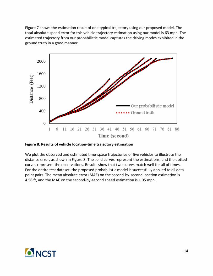
Figure 7 shows the estimation result of one typical trajectory using our proposed model. The total absolute speed error for this vehicle trajectory estimation using our model is 63 mph. The estimated trajectory from our probabilistic model captures the driving modes exhibited in the ground truth in a good manner.

Figure 8. Results of vehicle location-time trajectory estimation We plot the observed and estimated time-space trajectories of five vehicles to illustrate the distance error, as shown in Figure 8. The solid curves represent the estimations, and the dotted curves represent the observations. Results show that two curves match well for all of times. For the entire test dataset, the proposed probabilistic model is successfully applied to all data point pairs. The mean absolute error (MAE) on the second-by-second location estimation is 4.56 ft, and the MAE on the second-by-second speed estimation is 1.05 mph.

2000

1600

1200

800

400

0

Dis

tan

ce (f

eet)

15

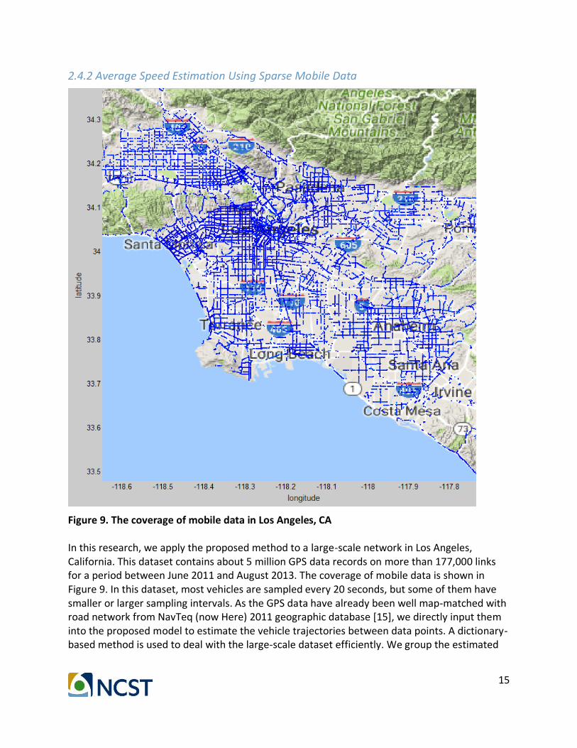
2.4.2 Average Speed Estimation Using Sparse Mobile Data

Figure 9. The coverage of mobile data in Los Angeles, CA In this research, we apply the proposed method to a large-scale network in Los Angeles, California. This dataset contains about 5 million GPS data records on more than 177,000 links for a period between June 2011 and August 2013. The coverage of mobile data is shown in Figure 9. In this dataset, most vehicles are sampled every 20 seconds, but some of them have smaller or larger sampling intervals. As the GPS data have already been well map-matched with road network from NavTeq (now Here) 2011 geographic database [15], we directly input them into the proposed model to estimate the vehicle trajectories between data points. A dictionary-based method is used to deal with the large-scale dataset efficiently. We group the estimated

16

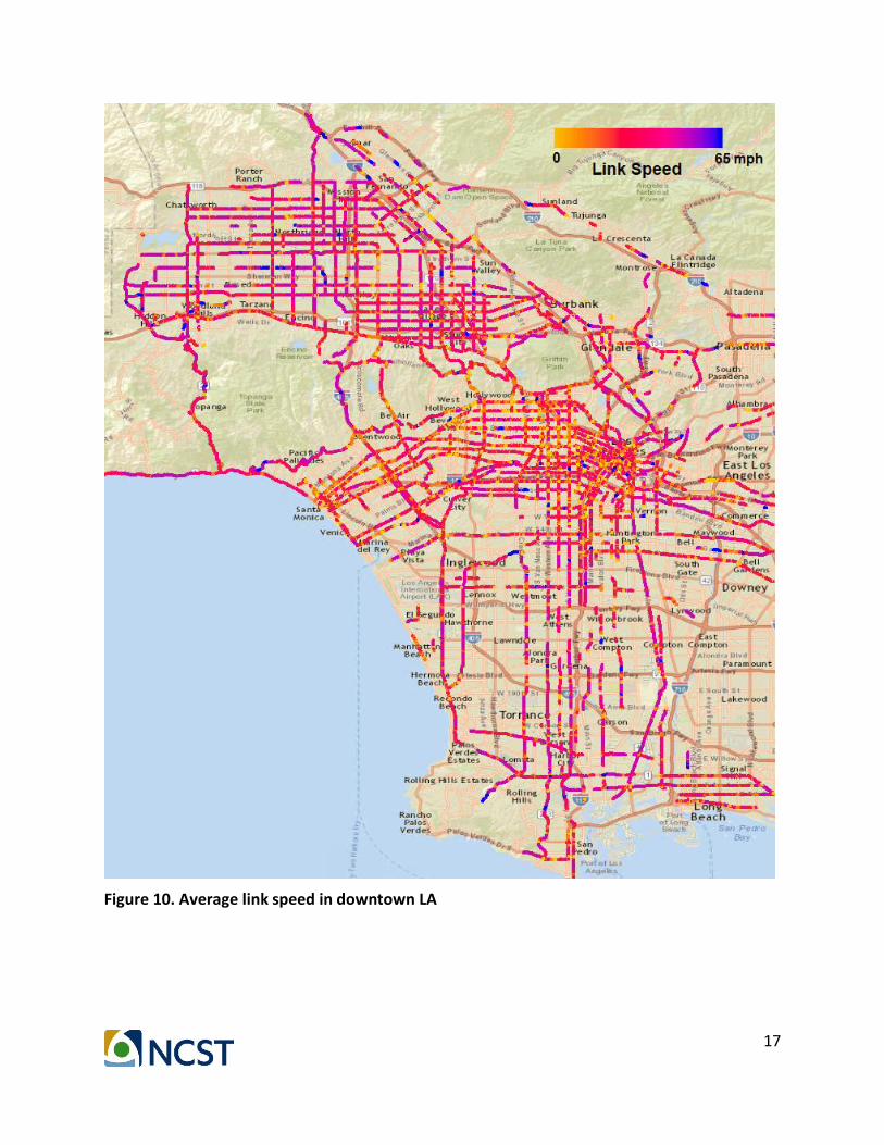
trajectories into each link to estimate link average speed, which is a key input for emission and dispersion modeling in following tasks. Based on the results from traffic state estimation, we visualize the average link speed using different colors in Figure 10. To match the link average speed with the road map, we get the corresponding longitude and latitude information for each data point using link id as indicator. We then calculate the average speed for each link by taking weighted vehicle average speed of the trip number. Using the centroid of each link as representative, we plot the average link speed (in mph) along with color map. As shown in the figure, traffic is more congested around the downtown and the coastal area (the average speed is lower than 20 mph), and less congested in the other zones.

17

Figure 10. Average link speed in downtown LA

18

3. Emission and Dispersion Estimation for Freeways

3.1 Emission Estimation using Mobile and PeMS data

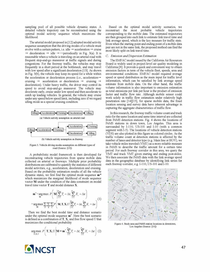
The previous section validates that sparse mobile crowed-sourced data can be utilized as a reliable source for traffic state estimation. In this section, we apply EMFAC and AERMOD to evaluate the air pollutant emissions and dispersion on freeways using traffic information acquired from mobile source and fixed location sensors. The EMFAC model issued by the California Air Resources Board (CARB) is widely used in project-level air quality modeling in California [8]. It provides a quick and convenient way to obtain emission factors in terms of the vehicle fleet, speeds, area and environmental conditions. The EMFAC model requires average speed or speed distribution as the main input for traffic level information, which can be satisfied by link average speed estimate from mobile data. On the other hand, the traffic volume information is also important to emission estimation as total emissions per mile per hour is the product of emission factor and traffic flow rate. Although mobile sensor could work solely in traffic flow estimation under relatively high penetration rate [16][17], for sparse mobile data, the fixed location sensing and survey data have inherent advantage in capturing the aggregate characteristics of traffic flow. For freeways in California, California Performance Measurement System (PeMS)[10] provides real time and historical traffic flow performance measures, such as traffic volume, average speed and truck ratio, at specific locations, but due to the relative spatial sparsity of detection stations, the traffic information between stations is unavailable. Especially at congested freeway bottlenecks during the peak hour, PeMS data may fail to capture the low speed and the stop-and-go behavior of vehicles. Figure 11 shows an example of the inconsistence between PeMS data and sample vehicle trajectories at freeway bottlenecks at SR-91. As shown in this figure, the PeMS speeds fit well with the vehicle speed at free flow sections. When the speed is around 40 mph, the probe speed curve oscillates around the PeMS station speed. For the heavy congestion area, the speed detection of PeMS stations may have large error to deal with the stop-and-go behaviors. In this case, mobile data would be an essential supplement to evaluate the traffic states at higher spatial resolution, and provide high-dimensional inputs for the following emission and dispersion models such as EMFAC and AERMOD. In this research, the freeway traffic volume count and truck ratio for the same location and same time interval are collected from PeMS detection stations. Figure 12 shows the locations of PeMS stations in downtown, Los Angeles. This area is surrounded by I-110, US-101 and I-10 (a shared segment with I-5). The locations of vehicle detection stations (VDS) are also plotted in this figure as colored circles. As the traffic volume counts at detection stations are affected by the number of lanes and detector type (e.g. Main line or HOV), we take vehicle miles traveled (VMT) as a more reliable measure in PeMS to describe the traffic amount for a certain time period. For each freeway corridor in this area, we query the VMT and truck VMT given starting and ending post-miles. We then associate the PeMS data with the link average speed data in

19

the geographic database by identifying link series for each freeway corridor, e.g. I-110, US-101 and I-10.

Figure 11. Speed trajectory of a probe vehicle and speeds at vehicle detection stations at SR-91

20

Source: PeMS website [10]

Figure 12. Study area and PeMS station locations in downtown, Los Angeles

21

3.2 Freeway Air Pollutant Visualization in ArcMap

Figure 13. PM 2.5 emissions per freeway link under PM peak traffic in August 2013 The traffic speed and volume data are applied to EMFAC2014 Web Database for emission estimation. As the sparse mobile data are collected between June 2011 and August 2013, we select the average traffic condition of PM peak hour (i.e. 5pm) in August 2013 as an example input. The calendar year and season in EMFAC are set to 2013/summer accordingly. We then configure the region to Los Angeles (MD) and generate the emission rate sheet for different speed intervals and different vehicle types. The air pollutant emissions are therefore calculated by pairing the emission rate sheet with average speed and volume data. Figure 13 shows the Fine particulate matter (PM 2.5) emissions for totally 439 link segments using different colors under PM peak traffic in August 2013. As the traffic condition of two directions of the freeway usually varies, the right hand side and left hand side of each freeway link have different colors in the figure. In AERMOD, we estimate the short-range dispersion of air pollutant emissions. First, the meteorological and terrain condition are defined in AERMET and AERMAP respectively as the background information. As emissions in this each link segment are treated as stable link source. The traffic-related emissions estimates from EMFAC are then spread out throughout each link in AERMOD to estimate the air pollutant concertation estimation. We finally plot the concertation contour map of each type of air pollutant in ArcMap [18]. Based on the freeway

22

emission source, we illustrates the PM 2.5 concentration of downtown LA in Figure 14. This figure clearly shows the high concentration around freeway corridors (especially interchanges) and visualizes the spatial dispersion of air pollutant. Note that only emissions from freeway traffic are taken into account in the Task. In the following task we will evaluate the impact of arterial traffic in emissions and dispersion.

Figure 14. PM 2.5 concentration in downtown LA for PM peak traffic in August 2013

23

4. Emission and Dispersion Estimation for Arterials

4.1 Emission Estimation for Arterials

In previous section, we developed air pollutant emission and dispersion models for freeways based on mobile data and Caltrans Performance Measurement (PeMS) data. That approach cannot be applied directly to urban arterials as most of the loop detector data is not available currently. Although mobile sensor could work solely in traffic flow estimation under relatively high penetration rate, the performance is not as good for sparse mobile data. The fixed location sensing and survey data have inherent advantage in capturing the aggregate characteristics of traffic flow. To find the alternative data source, we acquire Los Angeles traffic volume count data from LADOT database website. The traffic count data were collected manually or automatically by 2011-2013 from 2011 to 2013. The manual/automatic traffic count data cover most major intersections (highlighted by blue dots) in City of Los Angeles, especially in the downtown area as shown in Figure 15. Unfortunately, the count data for each single intersection only show one or two days’ daily volume based on 6-hour peak period count, so the emission and dispersion estimation results only represent the average level of air pollution in Los Angeles during 2011-2013. In addition to the count data, the sparse mobile crowd-sourcing data are used to 1) estimate average speed for each arterial link, and 2) estimate the distribution of traffic volume in a day to find the hourly volume for certain time of day.

24

Figure 15. Intersections with manual/automatic traffic counts in downtown, LA We then match the traffic count data with geographic database using the road name as the key words. Then, the estimated emissions for each link segment can be calculated by multiplying the average emission factors (considering the fleet composition and speed distribution) by the hourly volume in EMFAC. Finally, the dispersion impact at downwind locations of the arterials is derived by AMS/EPA Regulatory Model (AERMOD) and visualized in ArcMap. Based on the traffic count and mobile crowd-sourcing data, we apply EMFAC model to estimate the link-based vehicular emissions for urban arterials. Figure 16 shows the Fine Particulate Matter (PM 2.5) emissions for more than 3000 freeway and arterial link segments using different colors under PM peak traffic in August 2013. As the traffic condition of two directions of the freeway usually varies, the right hand side and left hand side of each freeway link have different colors in the figure.

25

Figure 16. PM 2.5 emissions per link under PM peak traffic in August 2013

26

4.2 Dispersion Estimation for Arterials

Based on both arterial and freeway emission source, we divide the research area into 57x71 grids and calculate the PM 2.5 concentration in AERMOD. Figure 17 illustrates the PM 2.5 concentration of downtown LA. This figure clearly visualizes the spatial dispersion of air pollutant. Air pollutants usually concentrate around freeway corridors (especially interchanges) and some busy arterials. The maximum PM 2.5 concentration rate for downtown LA area may reach 140 μg/m2 during the PM peak hour. For most links, the PM 2.5 concentration rate is below 30 μg/m2.

Figure 17. PM 2.5 concentration under PM peak traffic in August 2013 We then compare the estimated concentration with field measures from Quality Assurance Air Monitoring Station. As circled in Figure 17, there is one air monitoring site named as Los Angeles-North Main Street Station in the study area. The estimated PM 2.5 concentration is around 15 μg/m2 (colored as yellow) as this station is relatively far from high PM 2.5 concentration freeway and arterial network. We then query the ground truth from EPA AirData as shown in Figure 18, which indicates that the average daily mean PM2.5 concentration in

Los Angeles-North Main Street Station

27

August 2013 is about 13 μg/m2. As the peak hour concentration is usually higher than the daily mean, the numerical results show that the proposed system have good performance in air pollutant concentration estimation. This figure also shows that the Quality Assurance Air Monitoring Station may not well represent the surrounding area in measuring the air condition due to the sparsity of the stations and high diversity of the concentration rate.

Source: US EPA AirData [19]

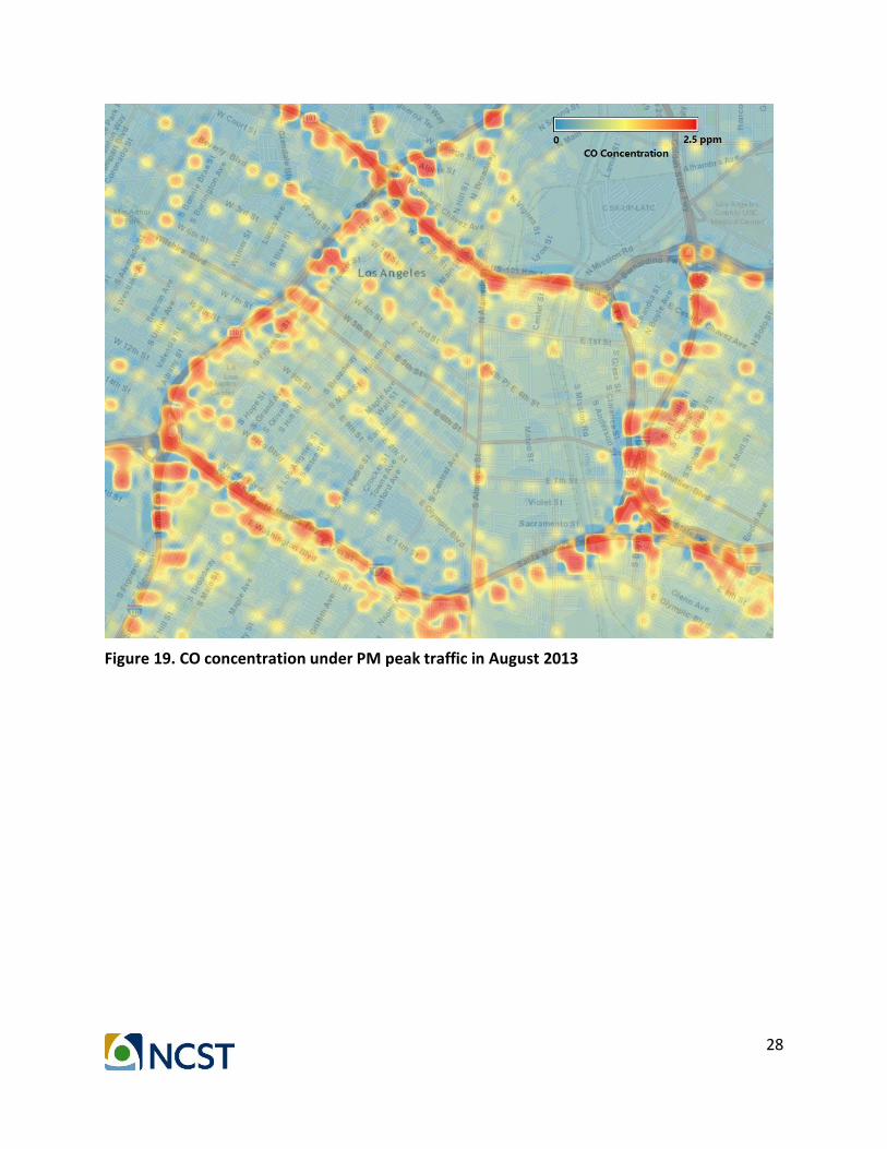
Figure 18. Daily Mean PM2.5 Concentration for Los Angeles-North Main Street Station Similar approaches are applied to other types of air pollutants. Figure 19 shows the concentration of Carbon monoxide and Figure 20 shows the concentration of NOx. In Section 5, the research team applied the proposed model to the broader area in the City of Los Angeles to investigate the impact of vehicular emission on different area of the city.

28

Figure 19. CO concentration under PM peak traffic in August 2013

29

Figure 20. NOx concentration under PM peak traffic in August 2013

30

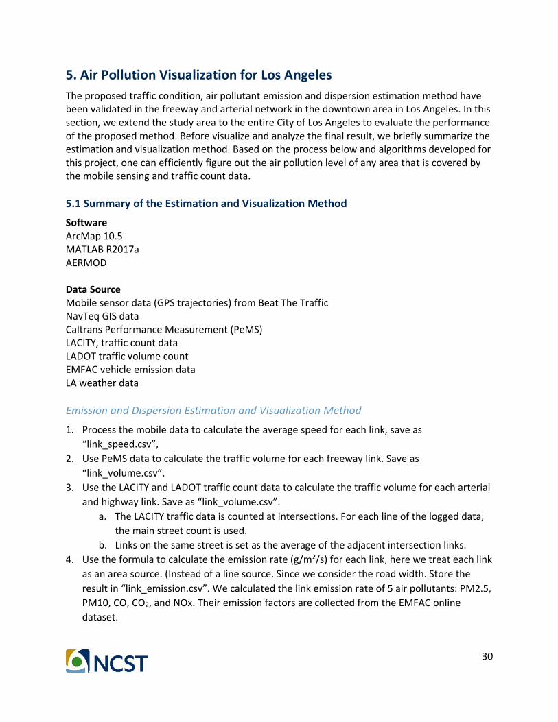
5. Air Pollution Visualization for Los Angeles

The proposed traffic condition, air pollutant emission and dispersion estimation method have been validated in the freeway and arterial network in the downtown area in Los Angeles. In this section, we extend the study area to the entire City of Los Angeles to evaluate the performance of the proposed method. Before visualize and analyze the final result, we briefly summarize the estimation and visualization method. Based on the process below and algorithms developed for this project, one can efficiently figure out the air pollution level of any area that is covered by the mobile sensing and traffic count data.

5.1 Summary of the Estimation and Visualization Method

Software ArcMap 10.5 MATLAB R2017a AERMOD Data Source Mobile sensor data (GPS trajectories) from Beat The Traffic NavTeq GIS data Caltrans Performance Measurement (PeMS) LACITY, traffic count data LADOT traffic volume count EMFAC vehicle emission data LA weather data

Emission and Dispersion Estimation and Visualization Method

1. Process the mobile data to calculate the average speed for each link, save as

“link_speed.csv”,

2. Use PeMS data to calculate the traffic volume for each freeway link. Save as

“link_volume.csv”.

3. Use the LACITY and LADOT traffic count data to calculate the traffic volume for each arterial

and highway link. Save as “link_volume.csv”.

a. The LACITY traffic data is counted at intersections. For each line of the logged data,

the main street count is used.

b. Links on the same street is set as the average of the adjacent intersection links.

4. Use the formula to calculate the emission rate (g/m2/s) for each link, here we treat each link

as an area source. (Instead of a line source. Since we consider the road width. Store the

result in “link_emission.csv”. We calculated the link emission rate of 5 air pollutants: PM2.5,

PM10, CO, CO2, and NOx. Their emission factors are collected from the EMFAC online

dataset.

31

Emission_rate [g/m2/s] = volume [veh/hr] * emission_factor [g/mile/veh] / road_width [m] / 1609.34 [m/mile] / 3600 [s/hr].

5. Combine “link_speed.csv”, “link_volume.csv” and “link_emission.csv” into one file

“link_info.csv” by “Link_ID”.

6. Use ArcMap to visualize the link average speed, link emission rate.

a. Import NevTech GIS data to ArcMap. (Add data)

b. Import “link_info.csv”. (Add data)

c. Join “link_info.csv” to NevTech data by “Link_ID”, only keep the matched links. This

step helps us to keep the links with sufficient data. Save the joined-data layer as

shape file “LA_links.shp”.

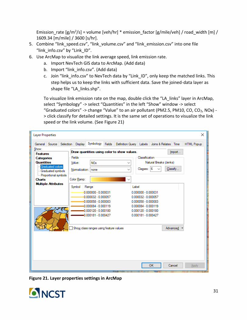
To visualize link emission rate on the map, double click the “LA_links” layer in ArcMap, select “Symbology” -> select “Quantities” in the left “Show” window -> select “Graduated colors” -> change “Value” to an air pollutant (PM2.5, PM10, CO, CO2, NOx) -> click classify for detailed settings. It is the same set of operations to visualize the link speed or the link volume. (See Figure 21)

Figure 21. Layer properties settings in ArcMap

32

7. Pre-process the link emission data for Aermod and use Aermod to model the emission

dispersion.

a. In ArcMap, search “project” to find the Data Management Tool “Project”. Project

the “LA_links” layer to “UTM Zone 11” Coordinates System. Name the projected

layer as “LA_links_projected”.

b. Search “add xy” to find the tool “Add Geometry Attributes”. Use the inputs shown

in the figure below to add the start, middle and end point to each link. (Add to the

table as attributes.)

5.2 Visualizing Air Pollution Level of Los Angeles

Based on the method summarized in Section 5.1, we visualize the annual peak hour air pollutant emissions and concentration for City of Los Angeles and its surrounding areas based on mobile data and traffic count data from 2011 to 2013. In Figure 22, we compare the PM2.5 concentration estimated from the proposed method (on the right) with the ground truth value from CalEnviroScreen 2.0 [20] (on the left). The CalEnviroScreen figure shows the PM2.5 annual mean monitoring data extracted from the monitoring sites from CARB’s air monitoring network database. Different colors represent the estimated concentration of the center of the ZIP code based on interpolation method. For both figures, the PM2.5 concentration has similar spatial distribution:

1) As one of the most polluted city in California, Los Angeles has high PM2.5 concentration in all of its ZIP codes;

2) The concentration is very high in the downtown area, and decreasing gradually in the surrounding region; and

3) That decreasing trend goes faster for the northwest direction. If we compare two locations with same distance to the downtown, the one in the southeast have higher concentration.

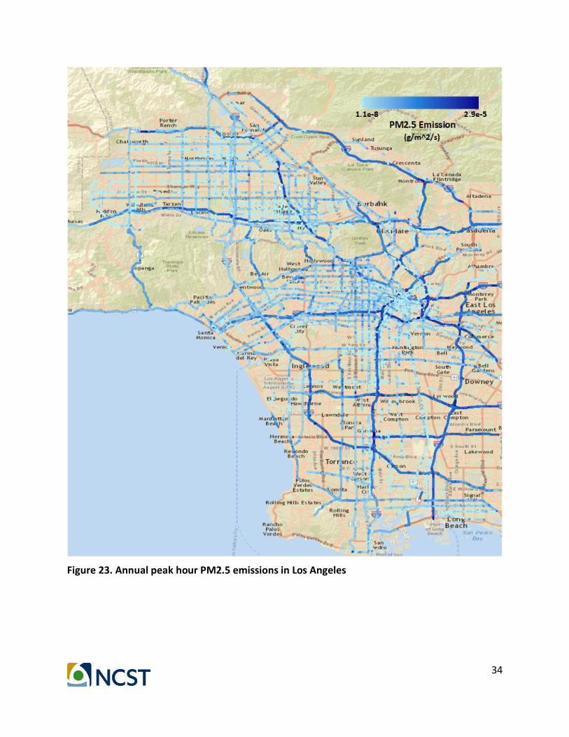
In addition, the PM2.5 concentration figure based on proposed method has higher resolution than the one in CalEnviroScreen. Instead of the average concentration of the whole ZIP code, the environmental impact of the congested links can be more clearly visualized by the proposed method. Figure 23 and 24 present the high definition version of the PM 2.5 emission map and concentration map. We also show NOx emission and concentration in Figure 25 and 26, along with CO2 emission and concentration in Figure 27 and 28.

33

Figure 22. PM2.5 concentration comparison between CalEnviroScreen and proposed method

Los Angeles Area

34

Figure 23. Annual peak hour PM2.5 emissions in Los Angeles

35

Figure 24. Annual peak hour PM2.5 concentration in Los Angeles

36

Figure 25. Annual peak hour NOx emissions in Los Angeles

37

Figure 26. Annual peak hour NOx concentration in Los Angeles

38

Figure 27. Annual peak hour CO2 emissions in Los Angeles

39

Figure 28. Annual peak hour CO2 concentration in Los Angeles

40

6. Conclusions

In this research, we develop a traffic-related air pollution evaluation system based on sparse mobile crowd-sourced data. To tackle the low frequency problem, the previously developed stochastic arterial trajectory estimation model is extended to freeways. Unique features of freeway driving modal activity are also considered. In response to the low penetration problem, we fuse the sparse mobile data with PeMS and LADOT traffic count data, which provide reliable real-world traffic volume information. The traffic state information for certain time intervals (e.g., peak hours) are applied to EMFAC model to estimate vehicular emissions. For freeways, traffic volume and truck ratio records collected from PeMS are also incorporated to the model to tackle the data sparsity problem. For arterials, the traffic volume information is acquired from either historical manual count or flow estimation methods. In AERMOD, we estimate the short-range dispersion of air pollutant emissions. The pollutant emission and dispersion are visualized in ArcMap. We further compare the estimated air pollutant concentration with the measurements from the air quality monitoring sites. It shows that the monthly peak hour PM 2.5 concentration matches well with the ground truth value, with error of 2 ug/m3. The estimated spatial distribution of annual PM 2.5 concentration is also similar to that from CalEnviroScreen. Due to the relatively sparsity of the air quality monitoring sites, CalEnviroScreen only provide average concentration of the whole ZIP code based on interpolation method. The proposed method can better visualize the environmental impact of the congested links with higher definition. Further improvement on the sparse mobile crowd-sourcing data-based air pollution evaluation method may include:

1) Currently, the mobile data source limits the effectiveness and timeliness of the proposed method. We will explore more updated and reliable mobile crowd-sourcing database (potentially with mobile air quality measurements) to validate the models and provide accurate air pollutant emission and concentration information.

2) We will further localize the air pollutant concentration down to each community, and investigate its livability by incorporating other pollution factors such as diesel particle matters and toxic releases from facilities.

3) This research will serve as a platform for other potential applications, such as eco-routing application which help reduce the driver and pedestrian’s exposure to air pollution, and connected vehicle based eco-signal timing.

4) The research team will further improve the computational efficiency in estimating the air pollutant emission and concentration and visualizing them in ArcMap.

41

7. References

[1] California Air Resources Board (CARB). The California Almanac of Emissions and Air Quality – 2013 Edition. http://www.arb.ca.gov/aqd/almanac/almanac.htm. Accessed on Mar 31, 2017.

[2] US Environmental Protection Agency (EPA). Near Roadway Air Pollution and Health. http://www3.epa.gov/otaq/nearroadway.htm. Accessed on Mar 31, 2017.

[3] California Air Resources Board (CARB). Estimate of Premature Deaths Associated with Fine Particle Pollution (PM2.5) in California Using a U.S. Environmental Protection Agency Methodology. August 2010

[4] R. Beelen, G. Hoek, , A. P. van den Brandt, R.A. Goldbohm, P. Fischer, et al. 2008. Long-Term Effects of Traffic-Related Air Pollution on Mortality in a Dutch Cohort (NLCS-AIR Study), Environmental Health Perspectives, vol. 116, no. 2.

[5] S. Samaranayake, S. Glaser, D. Holstius, J. Monteil, K. Tracton, E. Seto, A. Bayen, 2014. Real-Time Estimation of Pollution Emissions and Dispersion from Highway Traffic, Computer-Aided Civil and Infrastructure Engineering 29 (7), pp. 546–558.

[6] I.D. Greenwood, 2003. A new approach to estimate congestion impacts for highway evaluation-effects on fuel consumption and vehicle emissions (dissertation). The University of Auckland.

[7] K.S. Nesamani, L. Chu, M.G. McNally, R. Jayakrishnan, 2007. Estimation of vehicular emissions by capturing traffic variations. Atmospheric Environment 41 (14), 2996-3008.

[8] EMFAC2014 Web Database, https://www.arb.ca.gov/emfac/2014/. Accessed on Mar 31, 2017.

[9] AERMOD Modeling System, https://www3.epa.gov/ttn/scram/dispersion_prefrec.htm#aermod. Accessed on Mar 31, 2017.

[10] California Performance Measurement System (PeMS). http://pems.dot.ca.gov/. Accessed on Mar 31, 2017

[11] Current Count Data, http://ladot.lacity.org/what-we-do/traffic-volume-counts/current-count-data. Accessed on Mar 31, 2017

[12] P. Hao, K. Boriboonsomsin, G. Wu, & M. Barth, 2014. Probabilistic model for estimating vehicle trajectories using sparse mobile sensor data. IEEE Transactions on Intelligent Transportation Systems, 18(3), 701-711.

[13] P. Hao, G. Wu, K. Boriboonsomsin, and M. Barth, “Modal activity-based vehicle energy/emissions estimation using sparse mobile sensor data,” in Transportation Research Board 95th Annual Meeting, No 16-6861, 2016.

[14] Next Generation SIMulation, http://ngsim-community.org/. Accessed Apr 16, 2014.

42

[15] HERE Map Data, https://here.com/en/products-services/data/here-map-data. Accessed on Mar 31, 2017

[16] P. Hao, Z. Sun, X. Ban, D. Guo, and Q. Ji, “Vehicle index estimation for signalized intersections using sample travel times,” Transportation Research Part C, 36(1), 513-529, 2013.

[17] P. Hao, X. Ban, D. Guo, and Q. Ji, “Cycle-by-cycle queue length distribution estimation using sample travel times,” Transportation Research Part B, 68, 185-204, 2014.

[18] ArcMap. http://desktop.arcgis.com/zh-cn/arcmap/. Accessed on Mar 31, 2017.

[19] EPA Air Data. https://www.epa.gov/outdoor-air-quality-data/air-data-concentration-plot. Accessed on Mar 31, 2017.

[20] California Communities Environmental Health Screening Tool, Version 2. https://oehha.ca.gov/calenviroscreen/report/calenviroscreen-version-20, Accessed on Mar 31, 2017.

43

Appendix I: Acronyms and Abbreviations

AERMOD AMS/EPA Regulatory Model

AMS American Meteorological Society

CalEnviroScreen California Communities Environmental Health Screening Tool

CARB California Air Resources Board

EMFAC EMission FACtors Model

EPA Environmental Protection Agency

GPS Global Positioning System

LADOT City of Los Angeles Department of Transportation

MAE mean absolute error

NOx nitrogen oxides

NGSIM Next Generation SIMulation

PeMS California Performance Measurement System

PM particulate matter

44

Appendix II: Glossary

Sparse mobile sensor data: In this research, mobile sensor data represent the GPS data collected from the mobile devices. As the commercial GPS data usually have low sampling rate (collected 1 data point every 10-60 seconds) to limit the cost on data transmission and archiving, we can only have sparse mobile sensor data other than second-by-second GPS traces.

Vehicle trajectory: From the GPS logs, one can derive the vehicle’s spatial-temporal trace, which would indicate the movement of that vehicle. That trace is called vehicle trajectory.

Modal activity: The driving mode of the vehicle, including acceleration, deceleration, cruising, and idling.

Modal activity sequence: The sequence of all model activities in a certain time period, e.g. deceleration- idling- acceleration. In the proposed models we search for the “optimal” modal activity sequence which is the most probable one in a stochastic model.

Vehicle dynamic states: The vehicle’s location and speed in each second for a certain time period,

A prior probability distribution: In Bayesian statistical inference, a prior probability distribution, often simply called the prior, of an uncertain quantity is the probability distribution that would express one's beliefs about this quantity before some evidence is taken into account. (from wiki)

Gaussian Mixture Model: A Gaussian mixture model is a probabilistic model that assumes all the data points are generated from a mixture of a finite number of Gaussian distributions with unknown parameters. (from wiki)

45

Appendix III: Publication

A conference paper based on the proposed research was presented in The 5th Annual IEEE Conference on Technologies for Sustainability (SusTech 2017) in Phoenix, AZ on November 12-14, 2017. The full paper is attached in this appendix.

46

47

48

49

50

51