evaluating customer service representative staff ... · evaluating customer service representative...
TRANSCRIPT
Centre for Management of Technology and Entrepreneurship Faculty of Applied Science and Engineering
University of Toronto
Evaluating Customer Service Representative Staff Allocation and Meeting Customer Satisfaction Benchmarks: DEA Bank Branch Analysis
M.A.Sc Thesis
by
Elizabeth Jeeyoung Min
A thesis submitted in conformity with the requirements
for the degree of Masters of Applied Science Graduate Department of Chemical Engineering
University of Toronto
Supervisor
Dr. Joseph C. Paradi, Ph.D., P.Eng., FCAE
2011
Copyright by Elizabeth Jeeyoung Min, 2011
ii
ABSTRACT
Evaluating Customer Service Representative Staff Allocation and Meeting Customer Satisfaction Benchmarks: DEA Bank Branch Analysis
Elizabeth Jeeyoung Min
Masters of Applied Science Graduate Department of Chemical Engineering
University of Toronto
2011
Abstract
This research employs a non-parametric, fractional, linear programming method, Data
Envelopment Analysis to examine the Customer Service Representative resource allocation
efficiency of a major Canadian bank’s model. Two DEA models are proposed, (1) to evaluate
the Bank’s national branch network in the context of employment only, by minimizing Full
Time Equivalent (FTE) while maximizing over-the-counter (OTC) transaction volume; and
(2) to evaluate the efficacy of the Bank’s own model in meeting the desired customer
satisfaction benchmarks by maximizing fraction of transactions completed under
management’s target time. Non-controllable constant-returns-to-scale and variable-returns-
to-scale model results are presented and further broken down into branch size segments and
geographical regions for analysis. A comparison is conducted between the DEA model
results and the Bank’s performance ratios and benchmarks, validating the use of the proposed
DEA models for resource allocation efficiency analysis in the banking industry.

iii
ACKNOWLEDGEMENT I would like to express my sincere gratitude to Professor J. C. Paradi as this thesis could not
have been written without his support, guidance and motivation during the time I spent at
CMTE. His continuous encouragement and never ending inspiration made this research truly
possible.
I would also like to thank the Canadian bank under study for their kind cooperation and help
in providing me with the appropriate data, especially Dick. J. for the opportunity and his
enthusiasm, all his support and help.
I would also like to thank the other members of CMTE for providing such a great
environment to learn and grow, really making my stay at CMTE unforgettable and full of
great memories.
Lastly, I would like to thank my parents for their never-ending support and love, I sincerely
thank you all for providing me with this amazing opportunity and all your support, making
this moment possible.
iv
TABLE OF CONTENTS Abstract ..................................................................................................................................... ii
Acknowledgement ................................................................................................................... iii
Table of Contents .................................................................................................................... iv
List of Figures ......................................................................................................................... vii
List of Tables............................................................................................................................ ix
Executive Summary ................................................................................................................. 1
Chapter 1: ................................................................................................................................. 3
Introduction and Problem Statement ..................................................................................... 3
1.1 Objectives ........................................................................................................................ 6
1.2 Method of Approach ........................................................................................................ 6
Chapter 2: ................................................................................................................................. 8
Literature Review ..................................................................................................................... 8
2.1 Ratio Analysis: The Traditional Approach ...................................................................... 8
2.2 Frontier Efficiency Approach .......................................................................................... 9 2.2.1 Parametric Methods ................................................................................................ 10
2.2.1.1 Stochastic Frontier Analysis (SFA) ................................................................ 10 2.2.1.2 Distribution-Free Approach (DFA) ................................................................. 11 2.2.1.3 Thick Frontier Approach (TFA) ...................................................................... 11
2.2.2 Non-Parametric Methods ........................................................................................ 11 2.2.2.1 Data Envelopment Analysis (DEA) ................................................................ 11 2.2.2.2 Free Disposal Hull (FDH) ............................................................................... 12
2.2.3 Frontier Efficiency Method Comparisons .............................................................. 12
2.3 DEA in Bank Performance Evaluation .......................................................................... 13 2.3.1 Model Types by Objectives .................................................................................... 14 2.3.2 Model Variations .................................................................................................... 14
2.3.2.1 Constant returns to scale vs. Variable returns to scale .................................... 14 2.3.2.2 Input-Oriented vs. Output-Oriented ................................................................ 15 2.3.2.3 Multistage DEA Analysis................................................................................ 15
Chapter 3: ............................................................................................................................... 16
Data Envelopment Analysis (DEA) ...................................................................................... 16
3.1 DEA Theory and Mathematical Formulation ................................................................ 16
3.2 Constant Returns-to-Scale (CRS) Model ...................................................................... 18 3.2.1 Input-Oriented CRS Model ..................................................................................... 18 3.2.2 Output-Oriented CRS Model .................................................................................. 21
3.3 Variable Returns-To-Scale (VRS) Model ..................................................................... 21 3.3.1 Input Oriented VRS Model ..................................................................................... 22 3.3.2 Output Oriented VRS Model .................................................................................. 24
v
3.4 Slacks Based Model (SBM) .......................................................................................... 24
3.5 DEA Extensions ............................................................................................................ 25 3.5.1 Categorical and Non-discretionary (Non-controllable) Variables .......................... 25 3.5.2 Multiplier Constraints ............................................................................................. 26
3.6 Technical and Scale Efficiency ..................................................................................... 27
3.7 DEA Characteristics ...................................................................................................... 28 3.7.1 Advantages .............................................................................................................. 28 3.7.2 Disadvantages ......................................................................................................... 28
Chapter 4: ............................................................................................................................... 29
Bank’s Current Model (BCM) and Data Overview ............................................................ 29
4.1 Bank Overview .............................................................................................................. 29
4.2. Data Overview .............................................................................................................. 30
4.3 The Bank’s Current Staff Allocation Model (BCM) Overview .................................... 31 4.3.1 Definitions .............................................................................................................. 31 4.3.2 CSR Resource Allocation Process .......................................................................... 31 4.3.3 The Bank’s Current Model ..................................................................................... 32 4.3.4 Bank’s Current Performance Measurement Ratios ................................................ 34
4.4 Data Overview: Univariate Analysis ............................................................................. 35
Chapter 5: ............................................................................................................................... 40
DEA Model #1 Formulation and Results: Evaluating BCM’s Performance .................... 40
5.1 Data Employed .............................................................................................................. 40
5.2 Model Formulation: Evaluating the BCM’s performance ............................................. 41
5.3 Empirical Findings ........................................................................................................ 42 5.3.1 Model #1: Result for All Branches ......................................................................... 43 5.3.2 Model #1: Result grouped by Branch Size groups ................................................. 44 5.3.3 Model #1: Result grouped by Geographic Regions ................................................ 45 5.3.4 Comparison between Paid FTE and BCM Recommended FTE ............................. 46
5.4 Comparison with the Bank’s Performance Ratios ......................................................... 49
5.5 Chapter Summary .......................................................................................................... 52
Chapter 6: ............................................................................................................................... 54
DEA Model #2 Formulation and Results: Evaluating BCM’s Accuracy .......................... 54
6.1 Data Employed .............................................................................................................. 54
6.2 Model #2 Formulation: Evaluating BCM’s Accuracy .................................................. 55
6.3 Empirical Findings ........................................................................................................ 56 6.3.1 Model #2: Branches as DMUs ................................................................................ 58 6.3.2 Model #2: Branch by Hour as DMUs ..................................................................... 59
6.4 Comparison with the Bank’s internal metrics ............................................................... 60 6.4.1 Branch by Hour as DMUs ...................................................................................... 60
vi
6.5 Chapter Summary .......................................................................................................... 62
Chapter 7: ............................................................................................................................... 63
Conclusions and Findings ...................................................................................................... 63
7.1 Key Analytic Contributions to the Bank’s Management Process ................................. 63
7.2 Findings Summary and Conclusions ............................................................................. 64
Chapter 8: ............................................................................................................................... 67
Recommendations and Future Work ................................................................................... 67
8.1 Recommendations ......................................................................................................... 67
8.2 Future Work ................................................................................................................... 68
References ............................................................................................................................... 69
Glossary ................................................................................................................................... 75
vii
LIST OF FIGURES Figure 3.1 Graphical representation of the CRS model .......................................................... 20
Figure 3.2 Graphical representation of CRS and VRS models ............................................... 23
Figure 4.1 The Bank’s CSR Resource Allocation Process .................................................... 32
Figure 4.2 Distribution of Branches across different Geographic Regions ............................ 35
Figure 4.3 Distribution of Branches by Bank’s Branch Size Group ....................................... 36
Figure 4.4 Distribution of Branches by newly segmented Branch Size Group ...................... 37
Figure 4.5 Distribution of Total FTE by branch .................................................................... 37
Figure 4.6 Distribution of average # of weekly total transactions by branch ........................ 38
Figure 4.7 Distribution of average weekly # of business transactions by branch .................. 38
Figure 4.8 Distribution of branches by desired serve time ..................................................... 39
Figure 5.1 Model #1: List of Inputs, Outputs and Non-controllable variables ....................... 42
Figure 5.2 Model #1: CRS and VRS Efficiency Distribution for All Branches ..................... 44
Figure 5.3 Model #1: CRS and VRS Average Efficiency Distribution by Branch Size for All
Branches .................................................................................................................................. 45
Figure 5.4 Model #1: CRS and VRS Average Efficiency Distribution by Geographic Region
for All Branches ...................................................................................................................... 46
Figure 5.5 Actual Paid Model: List of Inputs, Outputs and Non-controllable variables ........ 46
Figure 5.6 Distribution Client Serve Ratio by Branch Size Group ......................................... 50
Figure 5.7 Distribution of Throughput Ratio by Branch Size Group ..................................... 50
Figure 5.8 Comparison between CRS DEA Efficiency Score vs. Client Serve Ratio ............ 51
Figure 5.9 Comparison between CRS DEA Efficiency score vs. Throughput Ratio .............. 51
Figure 6.1 Model #2: List of Inputs, Outputs and Non-controllable variables for Evaluating
Accuracy of BCM ................................................................................................................... 55
Figure 6.2 Distribution of Average Total Transactions per Branch by Day .......................... 56
Figure 6.3 Distribution of Average number of Transactions by Hour per Branch ................ 57
Figure 6.4 Model #2: Distribution of CRS DEA Efficiency Score – Branch as DMU ......... 58
Figure 6.5 Model #2: Distribution of CRS Efficiency Score = Branch by Hour as DMU .... 59
Figure 6.6 Distribution of % Transaction under 5 or 10 minutes (according to benchmark) 60

viii
Figure 6.7 CRS DEA Efficiency score vs. % of Bank Transactions under Benchmark: Branch
by the Hour as DMU ............................................................................................................... 61
ix
LIST OF TABLES Table 4.1 Bank’s Personal and Business Products and Services ............................................ 29
Table 4.2 List of Data provided by the Bank on their National Branch Network .................. 30
Table 4.3 List of Inputs, Outputs and Model Levers for the Bank’s Current staff allocation
Model (BCM) .......................................................................................................................... 33
Table 5.1 Model #1: CRS and VRS DEA Model Results for All Branches ........................... 44
Table 5.2 CRS DEA Model Result Comparison for Actual Paid model vs. BCM
Recommended (Model #1) ...................................................................................................... 47
Table 5.3 CRS DEA Result Comparison Grouped by Branch Size: Actual Paid vs. BCM FTE
(Model #1) ............................................................................................................................... 47
Table 5.4 CRS DEA Result Comparison Grouped by Region: Actual Paid vs. BCM
Recommended (Model #1) ...................................................................................................... 48
Table 5.5 Model #1: Summary of CRS and VRS result by Branch Size and Region ........... 52
Table 5.6 Model #1: Summary of CRS and VRS Average Efficiency Scores and Scale
Efficiency ................................................................................................................................ 53
Table 6.1 Model #2: CRS DEA Result for All Branches........................................................ 58
1
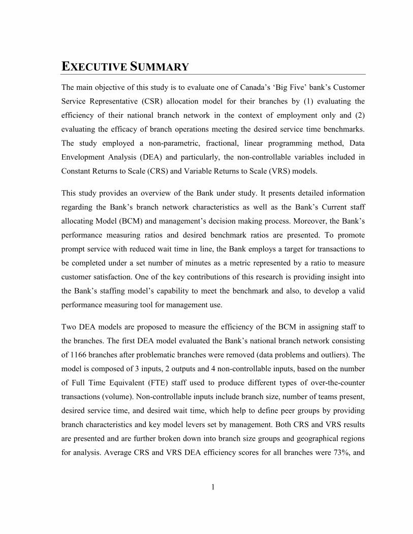
EXECUTIVE SUMMARY The main objective of this study is to evaluate one of Canada’s ‘Big Five’ bank’s Customer
Service Representative (CSR) allocation model for their branches by (1) evaluating the
efficiency of their national branch network in the context of employment only and (2)
evaluating the efficacy of branch operations meeting the desired service time benchmarks.
The study employed a non-parametric, fractional, linear programming method, Data
Envelopment Analysis (DEA) and particularly, the non-controllable variables included in
Constant Returns to Scale (CRS) and Variable Returns to Scale (VRS) models.
This study provides an overview of the Bank under study. It presents detailed information
regarding the Bank’s branch network characteristics as well as the Bank’s Current staff
allocating Model (BCM) and management’s decision making process. Moreover, the Bank’s
performance measuring ratios and desired benchmark ratios are presented. To promote
prompt service with reduced wait time in line, the Bank employs a target for transactions to
be completed under a set number of minutes as a metric represented by a ratio to measure
customer satisfaction. One of the key contributions of this research is providing insight into
the Bank’s staffing model’s capability to meet the benchmark and also, to develop a valid
performance measuring tool for management use.
Two DEA models are proposed to measure the efficiency of the BCM in assigning staff to
the branches. The first DEA model evaluated the Bank’s national branch network consisting
of 1166 branches after problematic branches were removed (data problems and outliers). The
model is composed of 3 inputs, 2 outputs and 4 non-controllable inputs, based on the number
of Full Time Equivalent (FTE) staff used to produce different types of over-the-counter
transactions (volume). Non-controllable inputs include branch size, number of teams present,
desired service time, and desired wait time, which help to define peer groups by providing
branch characteristics and key model levers set by management. Both CRS and VRS results
are presented and are further broken down into branch size groups and geographical regions
for analysis. Average CRS and VRS DEA efficiency scores for all branches were 73%, and
2
with scale efficiency ranging from 0.98 to 1.0, the study was able to conclude that the Bank
under study is operating at constant returns to scale.
CRS DEA results revealed that about 15% of the branches are efficient and measured a high
average efficiency score of 73% for the Bank’s branch network. This result suggests that the
BCM is, in fact, effective in allocating CSR resources across their national branch network
but there are still potential for improvements as DEA was able to identify inefficient
branches with efficiency scores ranging from 18% to the fully efficient, 100%.
The performance ratios used by the Bank were found to be not quite adequate to measure
branch efficiency as they both showed a positive correlation to the branch size. Thus, when
the performance ratio scores were compared to the DEA model efficiency scores, the result
was inconclusive as it suggested no significant correlation.
The second DEA model evaluated 20 branches from the pool of their national branch
network for which transaction-by-transaction timing data was available. This model is
composed of 2 inputs, 1 output and 1 non-controllable input, based on the number of FTE
staff used to produce transactions under 5 or 10 minutes depending on management’s desired
benchmark set for each branch. A two part analysis was conducted to evaluate each branch’s
efficiency as well as branch efficiency on an hourly average basis. Average CRS DEA
efficiency scores revealed to be 78% and 65%, respectively. From these results, it was
concluded that the BCM is effective in providing branch level staffing recommendations in
allocating CSR staff across the national branch network; however, it still needs improvement
in providing guidance on hourly staffing solutions.
DEA results were then compared to the Bank’s benchmark ratios. Correlation analysis
revealed strong positive correlation between the proposed DEA model efficiency score and
the Bank’s benchmark ratio with correlation coefficient of 0.70. This validates both the
Bank's BCM model and the proposed DEA model. The results suggest that DEA is, in fact, a
suitable tool to evaluate the Bank’s staff allocation model’s efficacy with respect to the
Bank’s desired benchmarks.
3
CHAPTER 1:
INTRODUCTION AND PROBLEM STATEMENT Canadian banks have a major influence not only on the country’s economic development, but
also on the entire society, owing to the increasing number of products and services aimed at
providing convenience and flexibility to clients’ finance options. The diverse client base,
ranging from individuals, to businesses, large corporations, governments, and non-profit
organizations, helps banks to grow and organize their assets. The banks handle
approximately 70% of total domestic assets in Canada, in which the ‘Big Five’ domestic
banks1 account for over 90% of the assets held by the banking industry, and operate through
an extensive network that includes over 5,300 branches across Canada [CANA03].
Due to changes in client needs and in response to growing demand for new financial
products, the products and services banks offer range from simple personal banking to
business, corporate banking, mutual funds, loans, mortgages and many others. Banks use
multiple channels to handle these transactions, including and not limited to online banking,
telephone banking, ABM and—most conventionally—through the branch network that
serves as the main contact with existing as well as potential clients. Despite the rapid rise in
the use of technology in banking, it was found that, in Canada, 61% of bank customers still
visited branches in person and on average made four trips per month [NFO03].
In all industries, businesses must continuously grow and evolve to remain competitive, and
large Canadian banks are no exception. In order for banks to remain competitive, it is
essential to improve on branch network performance, where the majority of the transactions
are still conducted, despite a number of alternative channels. The Bank in the present study is
a firm believer of providing customers with the attention needed by providing as much direct
contact with the customer service representatives as customers wish to have. Although the
banking industry is under pressure to develop and fund new access channels, optimizing
1 The ‘Big Five’ Banks are: “BMO Financial Group”, “CIBC”, “RBC Financial Group”, “ScotiaBank” and “TD
Bank Financial Group”.
4
branch operation is still one of the key elements in reducing costs and increasing customer
satisfaction. One of the major potential areas of improving branch network performance is
through better human resources management. Effective deployment of resources allows the
branch to perform at its best, thus meeting customer demand with the minimum required
resources.
The concept of resource optimization and evaluation is not new; however, the increasingly
complex products and services the banks presently offer have made evaluation of the
appropriate employee requirements for the branches rather difficult. In addition, client-driven
activities are usually difficult to predict, making staffing requirements challenging. Banks
traditionally evaluated their performance through different financial measurements; however
such conventional methods are often inconclusive and do not reflect the complex banking
industry well [GIOK08]. Banks traditionally used concepts, such as historical trends and
ratios, to measure efficiency; however, these analyses were usually two-dimensional
measurements, insufficient when the branch performance needs to be compared to that of
others. Moreover, such analyses fail to capture the multi-dimensionality and complexity of
different branch activities [ORAL90].
In this study, frontier analysis approach is suggested as it is one of the widely employed
methodologies to evaluate resource optimization for complex business units, such as bank
branches. This approach is more effective than traditional methods, since they evaluate the
branches’ relative efficiency against similar units and identify best performing units to build
a frontier for reference in lieu of just comparing to an average value. Data Envelopment
analysis (DEA), the frontier methodology employed in this thesis, is a non-parametric multi-
dimensional approach that is capable of identifying the best performer units as well as
recognizing complex relationships among the input and output components present in
today’s bank branch network. Among its most significant features is its ability to
simultaneously handle multiple indicators of performance as inputs and outputs, and thus,
provide an unbiased comparison of similar units without prior specifications of the unknown
underlying relationships. DEA's non-parametric nature determines its own model of the best
practice unit.

5
This thesis focused on developing a comprehensive methodology that evaluates the
efficiency of the branch staffing allocation process for one of the ‘Big Five’ banks in Canada.
Using a non-parametric linear programming method, this study attempted to evaluate the
Bank’s Current staff allocating Model (BCM) in regards to individual branch efficiency as
well as in comparison to the Bank’s desired benchmarks. The proposed DEA model
identifies the best practices of efficient branches, and evaluates the branch network across
Canada. Moreover, the results gained from the proposed efficiency score based on a DEA
analysis and the Bank’s own internal metrics were compared to each other for validation.
There are not many academic studies available to date that bring perspective to translating
efficiency in terms of customer satisfaction. Most studies in performance measurement just
focus on evaluating the current system and propose a methodology to effectively address
efficiency improvements rather than comparing them to a benchmark that is desired by the
management. The main objective of this research is to create a practical tool that has the
ability to first identify, and thereafter evaluate unique opportunities and situations to
potentially improve the staff allocation model, and providing a comparison to the Bank’ own
metrics to assess how well their model is performing against their benchmarks.
Identified best-practice technologies and policies can be implemented, while DEA can also
be used to determine which branches are most in need of restructuring, management
replacement or closure. Proposed DEA models have been integrated with the existing
planning tools utilized in the bank to establish policy guidelines in the planning,
implementation and execution stages of the best branch identification for the analysis.
This study was carried out by collaborating with one of the major Canadian banks, using the
data from their branch staff allocation model. The data collection and experimental
components have been supported and carried out in collaboration with the Manger of
Performance and Capacity Management. Throughout the research period, management has
been actively involved, provided specific data, internal documents on branch operations and
timely feedback.
6
1.1 Objectives
The objective of this study is to evaluate the Bank`s Current staff allocation Model (BCM)
by measuring the performance efficiency of the Bank`s branch network. Employing a non-
parametric linear programming method, Data Envelopment Analysis, this study attempted to
identify efficient branches against the Bank’s benchmarks and potential areas of
improvement in the model. There are two main parts to this study, (1) evaluating the BCM’s
performance to identify best performing branches and overall effectiveness of the current
model’s resource allocation across their national branch network, and (2) evaluating the
BCM’s accuracy in meeting desired benchmarks set by the Bank in regards to satisfying
customer demand.
By evaluating the model’s efficiency according to the desired benchmarks, management can
(1) discover areas of improvements in the model, leading to (2) identifying guidance on how
to determine the best staff mix in order to optimize resource allocation. The segregated
regional and branch size analysis result (3) identify regional and branch size characteristics
that needs to be employed to calibrate the model to fit different region and branch size
allocations.
1.2 Method of Approach
The following chapters present the design and implementation of the research methodology,
from its theoretical conception to its application.
• Chapter 2 – Literature Review, presents a detailed review of the relevant
literature focusing on branch performance assessment, including parametric and
non-parametric approaches.
• Chapter 3 –Overview of the Bank’s Current Model (BCM) and Data,
describes the BCM employed by the management to staff CSR team across its
branch network and an overview of statistical analysis on the data set.
7
• Chapter 4 – Data Envelopment Analysis, presents the research methodology,
describing the theoretical background for Data Envelopment Analysis (DEA). It
includes applicable DEA models: theory, terminology and mathematical
formulations, as well as their applications.
• Chapter 5 – DEA Model #1 Formulation and Results: Evaluating BCM’s
Performance, proposes the DEA model for BCM efficiency measurement and
also presents the DEA results and analysis.
• Chapter 6 – DEA Model #2 Formulation and Results: Evaluating BCM’s
Accuracy, proposes the DEA model for evaluating the accuracy of the BCM and
also presents comparison between the DEA’s result and the Bank’s internal
metrics.
• Chapter 7 – Conclusions and Future Work, concludes the thesis with the
summary of work done, as well as the theoretical and empirical contributions of
this research. The chapter also provides recommendations for future research.
8
CHAPTER 2:
LITERATURE REVIEW This chapter presents an overview of past and present literature on evaluating performance of
financial institutions at the corporate and branch levels. Ratio analysis marked the start of
performance measurement in the banking industry and it is still the most commonly used
method across different levels of management and decision-making processes in banks.
While traditional methods such as ratio analysis are still valid and useful, complexity in the
banking industry demanded a more sophisticated approach. In response, frontier
methodology is the emerging performance measurement approach, allowing more complex
use of information to provide insights into performance efficiency in the banking industry.
Frontier methodologies are categorized into two main areas, parametric and non-parametric
methods. This study uses Data Envelopment Analysis (DEA), one of the non-parametric
techniques introduced in this chapter. Data envelopment analysis is reviewed in detail in
Chapter 3.
2.1 Ratio Analysis: The Traditional Approach
Ratio analysis is the standard and historic method used by management to measure bank
performance [GIOK08]. Ratio analysis compares two parameters to understand their
relationship, offering insights into different aspects of bank operations, such as profitability,
liquidity, asset quality, risk management strategies, and more. Traditional accounting ratios
such as return on assets (ROA) and return on equity (ROE) have long been used to measure
bank performance. Ratio analysis is still the major performance measurement tool in many
industry settings, because it is simple to use and easy to compute and makes it possible to
quantify the change in relationship over time [GIOK08]. Although ratio analysis does offer useful insights into bank performance, it is often
incomplete and cannot represent the bank’s complex operation with its one-dimensional
nature. Only one aspect at a time can be compared and no single aspect of an organization
9
can fully characterize the operation of a business [FED03]. Studies have attempted to
combine ratios to form a more representative measure of bank performance; however such a
task has proven to be very complicated and can provide contradictory results depending on
different combinations [PARA04A]. Combining ratios is challenging since it is difficult to
determine suitable weights for each efficiency component (ratio) a priori, to establish a
representative combination [PARA11]. Another problem with ratio analysis is that it is
objectively difficult to determine how far above the average is inefficient or efficient
[GIOK08].
2.2 Frontier Efficiency Approach
The shortcomings of the traditional approaches have led to the development of a more
sophisticated approach in measuring operational performance. Production units are the units
in question for efficiency evaluation and in this particular study, bank branches. Frontier
analysis measures the relative efficiency of production units based on the distance from the
empirically estimated ‘best-practice’ frontier. Frontier efficiency analyses allow management
to objectively identify best practices in complex operational environments. There are five main approaches proposed in the literature as methods to evaluate bank
efficiency, namely, data envelopment analysis (DEA) as in Charnes and Cooper [CHAR78];
free disposal hull (FDH) as in Tulkens [TULK93]; stochastic frontier approach (SFA), also
called econometric frontier approach (EFA), as in Berger and Humphrey [BERG97]; thick
frontier approach (TFA) as in Berger and Humphrey [BERG91]; and distribution-free
approach (DFA) as in Berger, Hancock, and Humphrey [BERG93]; plus a rich literature on
all of these approaches and variations of them. There are two categories within the frontier efficiency analysis, they are parametric and non-
parametric linear programming approaches. Parametric approaches include SFA, TFA, and
DFA, and nonparametric approaches include DEA and FDH. These approaches primarily
differ in the assumptions on the data in terms of (a) how much restriction is imposed on the
specification of the best-practice frontier, and (b) the distributional assumptions imposed on
the random error and inefficiency [BERG97].
10
There are two efficiency measurements: technical efficiency, which focuses on the level of
inputs relative to the level of outputs; and economic efficiency, where a business has to
choose its input and/or output levels and a mix to optimize an economic goal, usually cost
minimization or profit maximization. This study measures technical efficiency, and price
data is not included in the branch-level analysis.
2.2.1 Parametric Methods
There are three main parametric methods: stochastic frontier analysis (SFA), distribution-free
approach (DFA), and thick frontier analysis (TFA). An advantage of the parametric methods
is that they allow for random error, thus reducing the chance of misidentifying error or
contamination of data as inefficiencies. Therefore the challenge in estimating with the
parametric method is accurately separating the random error from inefficiency. However, the parametric methods also have a disadvantage relative to the nonparametric
methods because of having to impose more structure on the shape of the frontier by
specifying a functional form for it [BAUE98]. The parametric model’s major weakness is
that there is a possibility of specifying the wrong functional form leading to inaccurate
efficiency estimates [GREB99].
2.2.1.1 Stochastic Frontier Analysis (SFA)
SFA has been the most-used parametric method since its introduction in 1977 by both Aigner
et al. [AIGN77] and Meeusen and Van Den Broeck, independently. SFA formulates a
frontier for a single input to multiple outputs or single output to multiple inputs scenarios.
The SFA models random error using a standard normal distribution with a mean of zero and
models inefficiency using an asymmetric half-normal distribution [BERG93]. The different
distributional patterns allow the error to be separated from the inefficiency. However, the half-normal distribution of inefficiency is relatively inflexible and assumes that
most units are clustered near full efficiency. Studies including that of Berger and Humphrey
[BERG97] have shown that specifying a more general truncated normal distribution for
inefficiency yields statistically significant, different results compared to the half-normal
11
distribution. However, such increased flexibility makes it difficult to separate inefficiency
from random error and shows a limitation to this approach.
2.2.1.2 Distribution-Free Approach (DFA)
DFA also specifies a functional form for the frontier. However, DFA assumes that random
error averages out to zero over time, while efficiency remains stable over time [BAUE98]. It
allows inefficiencies to adopt any distribution shape provided they remain non-negative. The
inefficiency of each unit is calculated as the difference between its average residual and the
average residual of a unit on the efficient frontier.
2.2.1.3 Thick Frontier Approach (TFA)
TFA uses the same functional form for the frontier as SFA, but measures the overall
efficiency rather than the efficiency of an individual unit and thus does not assume any
distribution in random error or inefficiency [BAUE98]. Therefore, units in the lowest
average-cost quartile are assumed to have above-average efficiency and form a thick frontier,
hence the name. Such a property reduces the effect of extreme points in the data, however
provides limited understanding of the individual unit’s efficiency.
2.2.2 Non-Parametric Methods
Non-parametric methods include data envelopment analysis (DEA) and free disposal hull
(FDH). Non-parametric methods impose less structure on the frontier but do not allow for
random error, allowing vulnerability to inaccurately classify units as inefficient while error is
present.
2.2.2.1 Data Envelopment Analysis (DEA)
DEA is a non-parametric linear programming methodology that develops production
frontiers and measures the relative efficiency of the units to these frontiers. The most
efficient units are those for which no other unit, or linear combination of units, has as much
or more of every output (given input) or as little or less of every input (given output)
12
[CHAR78]. The DEA frontier is formed as the piecewise linear combinations that connect
the set of these best-practice observations, yielding a convex production possibilities set.
DEA differs from its parametric counterparts in that it requires no explicit assumption or
knowledge about the relationship between inputs and outputs, and hence DEA does not
require any specification of the functional form of the frontier. However, DEA does not
account for random error, causing its frontier to be sensitive to the presence of outliers and
statistical noise [BAUE90]. As a performance measurement tool, DEA offers a strong ability to model complex and
multidimensional operations by being able to handle multiple inputs and multiple outputs
simultaneously. Unlike parametric methods that optimize a single regression plane through
all the data, DEA optimizes each unit individually. Furthermore, DEA does not require any
consistent metrics for its inputs and outputs, allowing varying scales to be compared
simultaneously.
2.2.2.2 Free Disposal Hull (FDH)
FDH is a variation of DEA where instead of the piecewise linear frontier normally
constructed; FDH constructs a stepwise frontier that measures efficiency only against real
units of observation [BERG97]. Since the FDH frontier is either identical to or interior to the
DEA frontier, FDH will typically generate larger estimates of average efficiency than DEA
[BERG97].
2.2.3 Frontier Efficiency Method Comparisons
There are many studies on bank performance and use of frontier efficiency approach to
measure performance, however there is not much information available to compare different
approaches as most studies have applied a single efficiency approach at a time. There are a
few studies that have compared multiple approaches, including Ferrier and Lovell [FERR90],
Bauer et al. [BAUE93], Hasan and Hunter [HASA96], Berger and Mester [BERG97],
Eisenbeis et al. [EISE97], Resti [REST97], and Berger and Hannan [BERG98].
13
There is no simple way to determine which of these methods best evaluates bank
performance. The choice of measurement method appears to strongly affect the calculated
efficiency and results have shown differences in ranking and inefficient unit percentages
depending on the method [BERG93]. However, depending on the problem at hand, different
methods offer advantageous edge in representing the relationship.
DEA has shown promising results in bank performance analysis ever since its introduction
and researchers have produced studies at exponential growth over the last 30 years
[EMRO08]. DEA gives a comparative ratio of the weighted sum of outputs to the weighted
sum of inputs for each unit under evaluation. The relative score expressed as a number
between 0 and 1 provides an efficiency measurement compared to the parametric methods,
such as Cobb-Douglas functions, which use statistical averages to construct a particular
measure of inefficiency, which may or may not be applicable to that unit’s composition
[LIU01]. Not only that, DEA’s ability to analyze multiple inputs and multiple outputs is a
strong advantage in evaluating a complex operation such as a bank. DEA with its non-
parametric properties, indicates an easier yet sophisticated approach to tackle an industry
problem, and was judged to be particularly suitable for this study. With the possibility of this
study being further developed into an industry tool, DEA was chosen to measure bank
performance in the current work. A detailed description of DEA models and theory follows
in Chapter 3.
2.3 DEA in Bank Performance Evaluation
DEA is by far the most commonly used operations research technique in assessing bank
performance. DEA was first introduced in 1978 by Charnes et al. and has been continuously
developed and explored in various applications not limited to the financial industry but
including health care, environmental studies, and more. At this time, there are a total of 163
studies that use DEA to assess bank efficiency and productivity. However, only 65 of these
provide branch-level analysis [PARA11]. Sherman and Gold were the first to publish a bank
branch network study using DEA, with a small sample data of 14 branches of a U.S. bank
[SHER85]. Compared to easily accessible bank level data that is available publicly, branch-
14
level data is scarce and involves the institution in the study, thus the number of branch-level
efficiency studies are much smaller in the literature compared to bank-level efficiency
studies. It is significant to note that this study evaluates one of the top five Canadian banks
and performs branch-level analysis on all currently operating branches across Canada, more
than 1200 branches. This section summarizes recent developments of DEA use in bank
studies over different model types and in literatures.
2.3.1 Model Types by Objectives
DEA branch-level studies can be classified into three model categories: production,
intermediation, and profitability [PARA04A] [GIOK08]. The production model attempts to
evaluate bank operations by using inputs such as labour and physical capital to produce
output transactions, such as loans and deposits. When costs are considered, the production
model evolves into a profitability model examining the operation's profitability of each
branch [PARA04A]. The intermediation model assumes that the bank is a financial
intermediary that transfers funds between savers and investors.
The production model is the most popular approach in bank analysis; many studies such as
Schaffnit et al. [SCHA97], Vassiloglou and Giokas [VASS90], and Parkan [PARK87] have
focused on developing production efficiency analyses using inputs of labour and computers,
and office space and number of transactions as outputs. This thesis is unique in that it
employed a production model but attempted to optimize customer satisfaction by reducing
the time it takes to complete a transaction.
2.3.2 Model Variations
2.3.2.1 Constant returns to scale vs. Variable returns to scale
DEA can be implemented by assuming either constant returns to scale (CRS) or variable
returns to scale (VRS). DEA started with a CRS model as proposed by Charnes et al.
[CHAR78] and this model has been used in studies such as Parkan [PARK87], who
evaluated a small sample (35 branches) of a large Canadian bank for operational efficiency
using a CRS model. In most recent studies, researchers have argued that CRS is only suitable
15
when all units under evaluation are operating at an optimal scale [FETH10]. Schaffnit et al.
[SCHA97] developed a VRS production efficiency model to examine 291 branches of a
major Canadian bank. Since that time other studies, including Cook et al. [COOK00] who
examined over 1300 Canadian branches, have increasingly used DEA models with the VRS
assumptions.
2.3.2.2 Input-Oriented vs. Output-Oriented
Technical efficiency can be estimated under either an input-oriented or output-oriented
approach. An input-oriented approach measures for a unit under evaluation, the amount of
input change to produce the same output and become efficient. In contrast, an output-
oriented approach measures for a unit under evaluation, the amount of output change needed
with the same input, to become efficient. By far, bank performance efficiency studies have
shown a strong tendency to use the input-oriented approach. This is because managers
assume that inputs such as labour and capital are more highly controllable compared to
common outputs such as profit, loans, and transactions [FETH10].
2.3.2.3 Multistage DEA Analysis
The two-stage concept in DEA was first introduced by Schinnar et al. [SCHI90] to measure
the performance of mental health care programs. The two-stage DEA method, where the
second stage uses the outputs of the first stage as its inputs, was applied by Wang et al.
[WANG97] to assess the impact of information technology on firm performance. Gradually,
use of the two-stage DEA method has increased in bank studies to analyze operations,
profitability, and marketability, such as in Chen [CHEN02], Luo [LUO03], and Ho and Zhu
[HO04], among others. Paradi et al. [PARA11] emphasizes the need to adopt two-stage
evaluation for bank branch efficiency analysis to simultaneously benchmark the performance
of operating units along different dimensions (production, profitability, and intermediation),
in order to satisfy different managers and executives for much practical industry application.
Paradi et al. [PARA11] developed a modified Slacks Based Measure model to aggregate the
obtained efficiency from stage one to generate a composite performance index for each unit.
16
CHAPTER 3:
DATA ENVELOPMENT ANALYSIS (DEA) This chapter presents an overview of the applied operations research technique used in this
study, known as Data Envelopment Analysis (DEA). It includes a brief overview of its
historical background, as well as detailed fundamental mathematical formulations and
theories commonly used in DEA efficiency studies.
DEA started from maximizing a simple ratio of a single output over single input. Farrell
[FARR57] introduced the concept of including multiple inputs and outputs and measuring
relative efficiency of units in terms of radial contractions or expansions from the inefficient
units to the efficient frontier. In general, there are two main DEA models used and they are
known as CRS and VRS. The CRS model was first developed in 1978 and was applied for
public sector and non-profit efficiency study as well as profit-oriented companies where the
value of the outputs were either known, or unavailable/incomplete [CHAR78]. The VRS
model was introduced in 1984 [BANK84]. Extensions to CRS and VRS model include
Slack-Based Model (SBM) as well as categorical, non-discretionary variables and multiplier
constraints as further discussed in this chapter.
3.1 DEA Theory and Mathematical Formulation
DEA defines a convex piecewise linear frontier composed of the ‘best-practice’ units which
all receive an efficiency score of 1, while the inefficient units are projected onto this efficient
frontier to calculate their efficiency score, which is less than 1. For each inefficient unit,
DEA provides a set of benchmarks of other similar but efficient units to compare, providing
useful information for management to recognize best practices as well as guidance on how to
improve inefficient units and benchmark targets for them [COOP07].
17
In order to produce meaningful efficiency scores, there are few criteria the data must meet
before the DEA analysis is done. Since DEA can be a benchmarking tool evaluating
inefficient DMUs by comparing them to other efficient units, it is required that a DMU is, in
fact, comparable in that they are similar in nature and operate in similar environments. As
discussed in Chapter 2, DEA does not account for random error and DEA’s frontier is very
sensitive to any measurement error, thus data must be thoroughly cleansed and all
irregularities must be removed before the analysis [BERG97]. Also, a sufficient number of
DMUs is needed to perform DEA. The number of degrees of freedom increases with the
number of DMUs and decreases with the number of inputs and outputs [COOP07]. As
proposed by Cooper et al, a general rule for the minimum number of DMUs (n) is that it
should exceed the greater of the product of the input (m) and output (s) variables or three
times the sum of the number of input (m) and output (s) variables [COOP07]:
� � ����� � ���� ��� (3.1)
Lastly, appropriate inputs and outputs must be chosen to represent the unit’s production
process as the model requires, including all the resources impacting the outputs and all useful
outcomes for evaluation. Furthermore, such inputs and outputs must be controllable by the
management to produce significant results that can be applied in the industry.
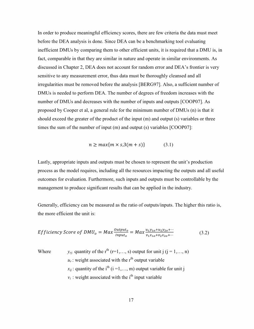
Generally, efficiency can be measured as the ratio of outputs/inputs. The higher this ratio is,
the more efficient the unit is:
������������������������ � ��� � !" !#$%" !# � ��� &'&#( )')#(*+&,&#(+),)#(*
Where yrj: quantity of the rth (r=1,…, s) output for unit j (j = 1,…, n)
ur : weight associated with the rth output variable
xij : quantity of the ith (i =1,…, m) output variable for unit j
vi : weight associated with the ith input variable
(3.2)
18
3.2 Constant Returns-to-Scale (CRS) Model
The CRS model is the first formulated DEA model as introduced by Charnes, Cooper and
Rhodes [CHAR78]. The CRS model is built on the assumption that constant returns-to-scale
(CRS) operation applies, implying that any increase in inputs results in proportional increase
in outputs, regardless of the scale of operation. The CRS model finds a set of weights for
each DMU that makes the DMU look as favourable as possible [CHAR78]. The goal of the
model is to maximize the efficiency score (θ) where every DMU uses total Xj = {xij} amount
of inputs to produce Yj = {yrj} of outputs. Each DMU’s efficiency score is calculated relative
to the other DMU’s efficiency score and it would only be considered efficient, when its score
equals to 1 and both slacks from the efficiency: s- and s+, are zero; otherwise, the DMU could
be inefficient and the efficiency score will vary between 0 and 1. A DMU can be weakly
efficient with a score of 1 even if slacks do exist. There are two orientations to CRS models
and they are input orientation and output orientation.
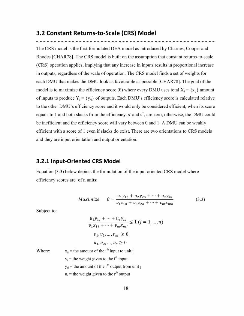
3.2.1 Input-Oriented CRS Model
Equation (3.3) below depicts the formulation of the input oriented CRS model where
efficiency scores are � of n units:
������-��������. � /0�0� /1�1� * /2�2�30�0� 31�1� * 34�4�
Subject to:
/0�05 * /2�2530�05 * 34�45 6 7��8 � 79 ��
30 31 9 34 �� :; /0 /1 9 /2 � :�Where: xij = the amount of the ith input to unit j
vi = the weight given to the ith input
yrj = the amount of the rth output from unit j
ur = the weight given to the rth output
(3.3)
19
The above fractional CRS model can be transformed into the following less computationally
intensive linear formulations: the primal and dual forms. CRS Input-Oriented Primal (3.4) CRS Input-Oriented Dual (3.5)
<=> + �������������?� � /0�0� * /2�2� ��� �������������������.
Subject to: 30�0� * �34�4� � 7 Subject to: .�@� �A �@5B5%5C0
A /D�D5EFC0 G�A 3@�@5HIC0 6 : �D� 6 A �D5B5%5C0
8 � 79 � � � 7 9 �
30 31 9 34 �� :; � � 7 9 �
/0 /1 9 /2 � : B5 � : The dual form uses a set of non-negative intensity variables, λ, to represent the weight of
each of the n DMUs. The initial optimization is performed once for each DMU to reduce all
inputs equally proportionally, bringing these DMUs closer to the frontier. Thus, optimality is
achieved by minimizing inputs by a factor of θ and indicates that inefficient DMUs would
only require θ amount (in percentage) of the inputs to produce the same amount of output.
CRS models are radial models, as their goal is to adjust inputs or outputs (in the case of
output orientation) radially from the origin. However, further input decreases or output
increases may still be possible after radial optimization has been achieved.
Input excesses, s-, and output shortfalls, s+, are known as input and output slack variables,
respectively, and are optimized in a second phase, where θ* is the optimal radial contraction
computed from the initial phase (3.4) :
<=>������ �����������J � A �@K4@C0 A �D(2DC0
Subject to: �@K � .L�@� G A �@5B5 �4@C0 ������� � 79�@( � A �D5B5 G �D������ � 79 ��2DC0B5 � :��8 � 79 �� �@K � :��� � 79 �� �D( � :��� � 79 ���
(3.6)
��
20
Existence of slack represents mix inefficiency and therefore a DMU is fully technically
efficient if any only if θ* = 1 (radial efficiency) and s+* = s-* = 0 (zero slacks). However, if
only θ* = 1 with nonzero slacks then the DMU is radially efficient with mix inefficiencies.
An inefficient DMU can be improved by referring its inefficient behaviour to the efficient
frontier formed by Eo, the reference set of DMUo composed of efficient DMUs. This
improvement is a projection to the point (>NO PNO) on the frontier where:
>NIO � .L�@� G �@K � A �@5B5L�5QR# 6 �@������S � 79 <�
PNTO � �D� �D( � A �D5B5L�5QR# � �D������U � 79 V� (WNX YNX) are the coordinates of a virtual linear composite DMU (i.e. AZ[\]^] where
are efficient and ^] are proportionality weights for DMUi) used to evaluate the perfor
of DMUo. It represents the target for efficient production that DMUo should strive fo
[COOP07].
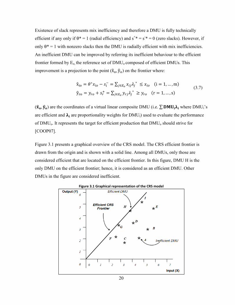
Figure 3.1 presents a graphical overview of the CRS model. The CRS efficient fronti
drawn from the origin and is shown with a solid line. Among all DMUs, only those a
considered efficient that are located on the efficient frontier. In this figure, DMU H i
only DMU on the efficient frontier; hence, it is considered as an efficient DMU. Othe
DMUs in the figure are considered inefficient.
Figure 3.1 Graphical representation of the CRS model
(3.7)
DMUi’s
mance
r
er is
re
s the
r
21
3.2.2 Output-Oriented CRS Model
The output oriented CRS model aims to maximize outputs at the same observed input values.
The primal and dual formulations are:
CRS Output-Oriented Primal (3.8) CRS Output-Oriented Dual (3.9)
Minimize A _I>IOHIC0 Maximize η
Subject to A `TPTO � 7ETC0 Subject to >IO � A >IaµabaC0
A `TPTa G A _I>IaHIC0 6 :ETC0 ηPTO 6 A PTaµabaC0
c � 79 d S � 7 9 <
_0 _1 9 _H � : U � 79 V `0 `1 9 `E � : µa � :
The input eK and output e( slacks of the output-oriented model are calculated in a second
phase:
eIK � >IO G A >IaµaHIC0 ��������������S � 79 <�
eT( � A PTaµaETC0 G ηLPTO����������U � 79 V� Where ηL is the optimal expansion from the first phase and eKL � EfL
θL ande(
A DMU is CRS fully efficient if and only if ηL � 7 and all optimal slacks a
inefficient DMUs, the following CRS projection can be used to improve (>NO >NIO � >IO G eIKL������S � 79 <�
PNIO � ηLPTO eI(L������U � 79 V�
3.3 Variable Returns-To-Scale (VRS) Model
The VRS model was first formulated by Banker, Charnes and Cooper in 19
variable returns-to-scale DEA formulation [BANK84]. The VRS model def
linear convex efficient frontier composed of the best performing DMUs. In
and outputs, the frontiers are encapsulated in a convex hull of efficient DM
model is formulated similarly to CRS but the addition of a variable (ijO) to t
(3.10)
L � EgLθL .
re zero. For
PNO�h
(3.11)84 and provides
ines a piecewise
multiple inputs
Us. The VRS
he model,
22
accounts for the economies of scale. In cases that a unique optimal solution is present,
ijO k : shows that the units are operating under increasing returns-to-scale while ijO � :
indicates constant returns-to-scale and ijO l : indicates decreasing returns-to scale.
3.3.1 Input Oriented VRS Model
Equation (3.12) below depicts the formulation of input oriented VRS model where efficiency
scores (�) of n units are maximized:
������-��. � A /D2DC0 �D� G /j�A 3@�@�4@C0
Subject to:
A /D2DC0 �D5 G /j�A 3@�@54@C0
6 7 8 � 79 �
/D �� :; � � 79 �
3@ �� :; � � 79 �
/j�h ����������m�
Like the CRS model, the above fractional VRS model can be transformed in
convenient computational forms: the primal and dual formulations. The maj
between CRS dual (eq.3.5) and VRS dual formulations is that the sum of na equal one.
VRS Input-Oriented Primal (3.13) VRS Input-Oriented D
Maximize o � A iTPTO G ijOETC0 Minimize θpFq
Subject to A rI>IOHIC0 � 7 Subject to θpFq>IO A iTPTaETC0 GA rI>IaHIC0 G ijO 6 : PTO 6 Aba c � 79 d A nabaC0 � iT rI � : S � 7 9 /j�h ����������m� U � 79
(3.12)
to more
or difference
variables must
ual (3.14)
� A >IanabaC0
PTanaC0
7���na � :� <
V
23
As previously demonstrated, slacks (3.6) can be incorporated in a second phase to measure
mix inefficiencies:
VIK � θpFqL>IO G A >IanaHIC0 ���S � 79 <�
VT( � A PTanaETC0 G PTO�������������U � 79 V���
A DMU is VRS–efficient if and only if θpFq � 7 and has zero slacks (V(L � VKL � :). The
target projection can be obtained by (>NO PNO� :
>NIO � θpFq>IO G VIKL������S � 79 <�
PNIO � PTO VI(L������U � 79 V�
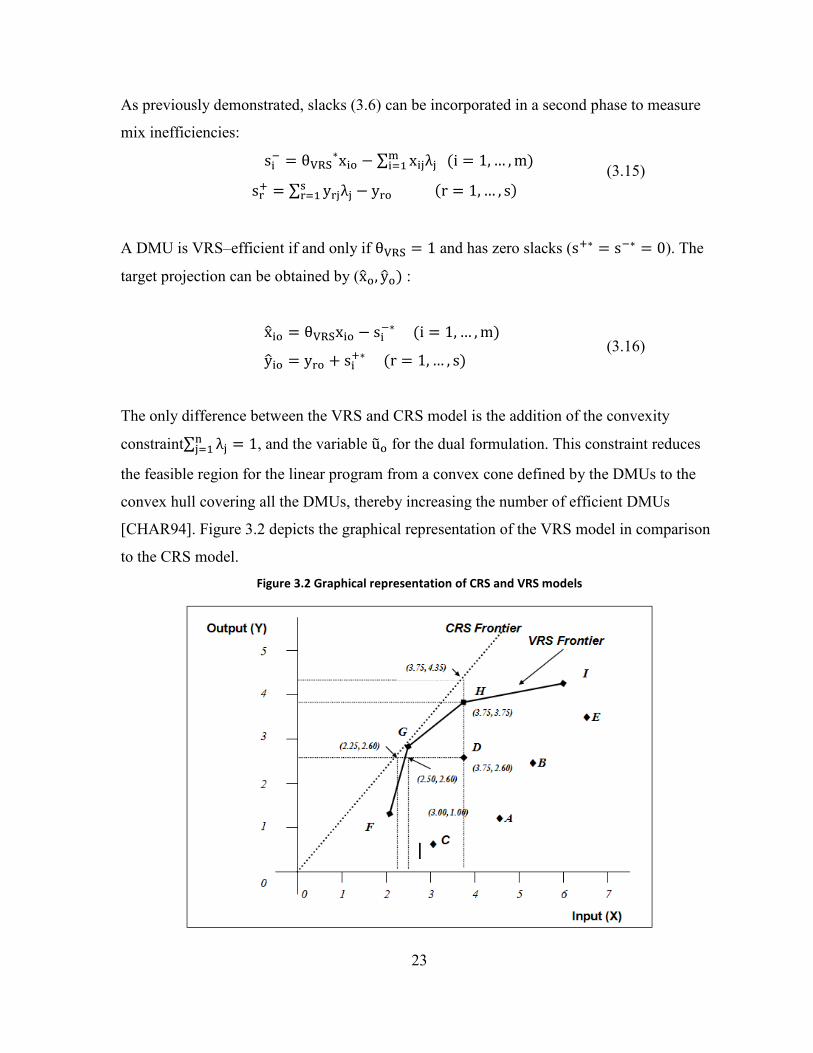
The only difference between the VRS and CRS model is the addition of the
constraintA nabaC0 � 7, and the variable ijO for the dual formulation. This co
the feasible region for the linear program from a convex cone defined by th
convex hull covering all the DMUs, thereby increasing the number of effic
[CHAR94]. Figure 3.2 depicts the graphical representation of the VRS mod
to the CRS model.
Figure 3.2 Graphical representation of CRS and VRS models
(3.16)
(3.15)
convexity
nstraint reduces
e DMUs to the
ient DMUs
el in comparison
24
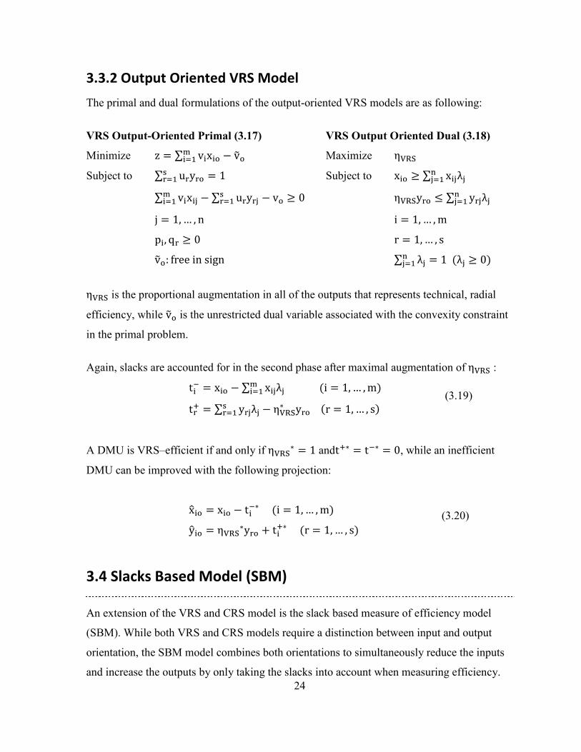
3.3.2 Output Oriented VRS Model
The primal and dual formulations of the output-oriented VRS models are as following:
VRS Output-Oriented Primal (3.17) VRS Output Oriented Dual (3.18)
Minimize o � A rI>IO G rjOHIC0 Maximize spFq
Subject to A iTPTOETC0 � 7 Subject to >IO � A >IanabaC0
A rI>IaHIC0 G A iTPTa G rOETC0 � : spFqPTO 6 A PTanabaC0
c � 79 d S � 7 9 <
_I `T � : U � 79 V rjOh tUuu�Sd�VSvd A nabaC0 � 7���na � :� spFq is the proportional augmentation in all of the outputs that represents technical, radial
efficiency, while rjO is the unrestricted dual variable associated with the convexity constraint
in the primal problem.
Again, slacks are accounted for in the second phase after maximal augmentation of spFq :
eIK � >IO G A >IanaHIC0 ��������������S � 79 <�
eT( � A PTanaETC0 G spFqL PTO�����U � 7 9 V�
A DMU is VRS–efficient if and only if spFqL � 7 ande(L � eKL � :, while an inefficient
DMU can be improved with the following projection:
>NIO � >IO G eIKL������S � 79 <�
PNIO � spFqLPTO eI(L������U � 79 V�
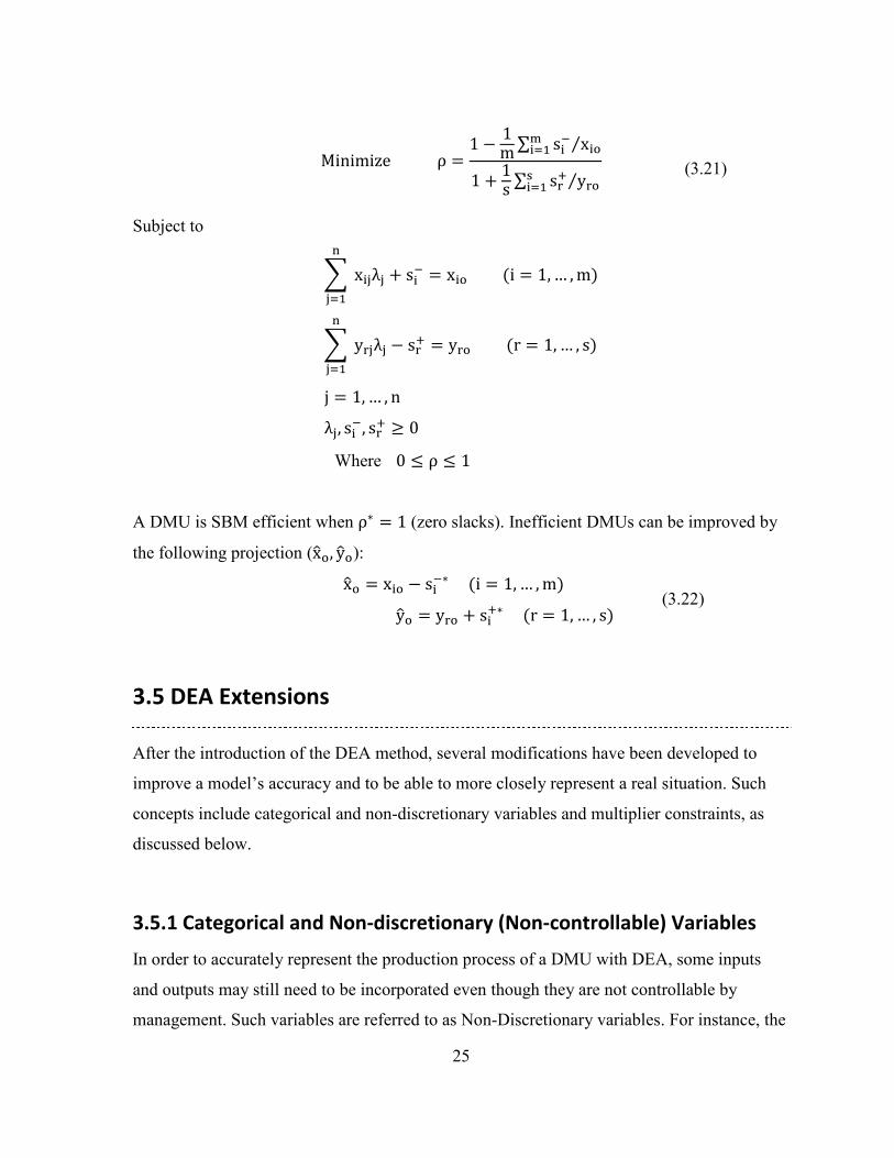
3.4 Slacks Based Model (SBM)
An extension of the VRS and CRS model is the slack based measure of effic
(SBM). While both VRS and CRS models require a distinction between inpu
orientation, the SBM model combines both orientations to simultaneously re
and increase the outputs by only taking the slacks into account when measur
(3.20)
i
t
d
in
(3.19)
ency model
and output
uce the inputs
g efficiency.
25
wSdS<Sou������������x � 7 G 7<A VIK >IOyHIC0
7 7V A VT( PTOyEIC0
Subject to
z�>Ianab
aC0 VIK � >IO����������S � 79 <�
z�PTanab
aC0G VT( � PTO����������U � 79 V�
c � 79 d
na VIK VT( � :
Where : 6 x 6 7
A DMU is SBM efficient when xL � 7 (zero slacks). Inefficient DMUs can be improved by
the following projection (>NO PNO):
>NO � >IO G VIKL������S � 79 <�
PNO � PTO VI(L������U � 7 9 V�
3.5 DEA Extensions
After the introduction of the DEA method, several modifications have bee
improve a model’s accuracy and to be able to more closely represent a rea
concepts include categorical and non-discretionary variables and multiplie
discussed below.
3.5.1 Categorical and Non-discretionary (Non-controllable
In order to accurately represent the production process of a DMU with DE
and outputs may still need to be incorporated even though they are not con
management. Such variables are referred to as Non-Discretionary variable
(3.22)
n d
l sit
r co
) V
A,
tro
s. F
(3.21)
eveloped to
uation. Such
nstraints, as
ariables
some inputs
llable by
or instance, the
26
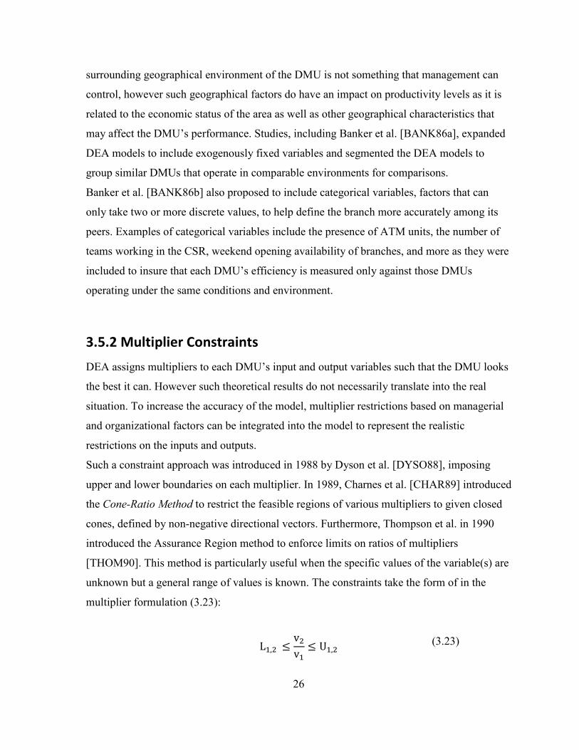
surrounding geographical environment of the DMU is not something that management can
control, however such geographical factors do have an impact on productivity levels as it is
related to the economic status of the area as well as other geographical characteristics that
may affect the DMU’s performance. Studies, including Banker et al. [BANK86a], expanded
DEA models to include exogenously fixed variables and segmented the DEA models to
group similar DMUs that operate in comparable environments for comparisons.
Banker et al. [BANK86b] also proposed to include categorical variables, factors that can
only take two or more discrete values, to help define the branch more accurately among its
peers. Examples of categorical variables include the presence of ATM units, the number of
teams working in the CSR, weekend opening availability of branches, and more as they were
included to insure that each DMU’s efficiency is measured only against those DMUs
operating under the same conditions and environment.
3.5.2 Multiplier Constraints
DEA assigns multipliers to each DMU’s input and output variables such that the DMU looks
the best it can. However such theoretical results do not necessarily translate into the real
situation. To increase the accuracy of the model, multiplier restrictions based on managerial
and organizational factors can be integrated into the model to represent the realistic
restrictions on the inputs and outputs.
Such a constraint approach was introduced in 1988 by Dyson et al. [DYSO88], imposing
upper and lower boundaries on each multiplier. In 1989, Charnes et al. [CHAR89] introduced
the Cone-Ratio Method to restrict the feasible regions of various multipliers to given closed
cones, defined by non-negative directional vectors. Furthermore, Thompson et al. in 1990
introduced the Assurance Region method to enforce limits on ratios of multipliers
[THOM90]. This method is particularly useful when the specific values of the variable(s) are
unknown but a general range of values is known. The constraints take the form of in the
multiplier formulation (3.23):
{01� 6r1r0 6 |01
(3.23)
27
3.6 Technical and Scale Efficiency
DEA results include technical and scale efficiency, target projections for the DMUs, as well
as their returns-to-scale’s level of operation, which all are essential information for the
analysis.
The CRS DEA model assumes a constant returns-to-scale (CRS) production for the DMUs,
meaning that scale of production does not affect efficiency. Hence, it only considers one
efficiency score, called the overall technical efficiency. The VRS DEA model assumes
variable returns-to-scale (VRS) production for the DMUs, measuring both scale efficiency
and technical efficiency. Scale Efficiency measures each DMUs distance from its optimal
scale size, by dividing the CRS efficiency by the VRS efficiency.
Figure 3.2 shows technical efficiency and scale efficiency concepts for both CRS and VRS
DEA models. The dashed line from the origin is representing the CRS frontier and the solid
line is showing the VRS frontier.
DMU G is located on both efficiency frontiers. It is CRS efficient as it is the only producer
on the CRS frontier. It also exhibits the highest average productivity, i.e., highest output per
input or slope, for its given input and output mix. Therefore, G is referred to as an efficient
DMU that is operating at its most productive scale size (MPSS) [BANK84]. VRS Frontier
(solid line) is built on DMUs: F, G, H, and I. All these DMUs are technically efficient,
however, only G is scale efficient, as it is the only DMU that is operating at constant returns-
to-scale. Therefore, G is considered both technically efficient and scale efficient, operating at
the MPSS. Cooper et al. [COOP07] provides a detailed explanation of MPSS term.
28
3.7 DEA Characteristics
3.7.1 Advantages
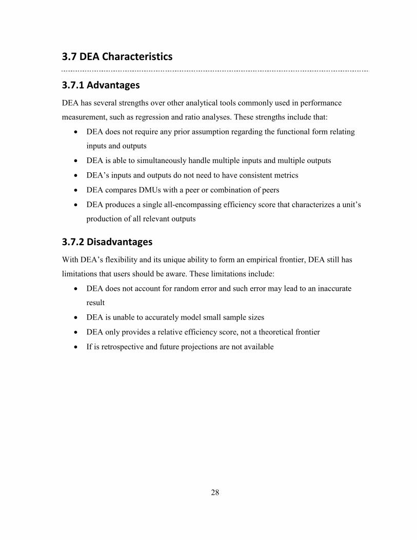
DEA has several strengths over other analytical tools commonly used in performance
measurement, such as regression and ratio analyses. These strengths include that:
• DEA does not require any prior assumption regarding the functional form relating
inputs and outputs
• DEA is able to simultaneously handle multiple inputs and multiple outputs
• DEA’s inputs and outputs do not need to have consistent metrics
• DEA compares DMUs with a peer or combination of peers
• DEA produces a single all-encompassing efficiency score that characterizes a unit’s
production of all relevant outputs
3.7.2 Disadvantages
With DEA’s flexibility and its unique ability to form an empirical frontier, DEA still has
limitations that users should be aware. These limitations include:
• DEA does not account for random error and such error may lead to an inaccurate
result
• DEA is unable to accurately model small sample sizes
• DEA only provides a relative efficiency score, not a theoretical frontier
• If is retrospective and future projections are not available
29
CHAPTER 4:
BANK’S CURRENT MODEL (BCM) AND DATA OVERVIEW This chapter provides an overview of the Bank and the BCM. The Bank under study employs
a complex staff allocation model based on a queuing algorithm, to estimate the sufficient
number of CSR employees for each branch on an annual basis. This section elaborates on
BCM and presents statistical analysis performed on the data set to fully understand the
properties and characteristics of the data and to determine suitable variables for the DEA
models (Chapter 5 and Chapter 6).
4.1 Bank Overview
The collaborating Bank under study is one of the ‘Big Five’ Canadian banks, currently
ranked in the top 100 banks worldwide in terms of asset size [CANA03]. The Bank offers an
extensive range of financial products and services to customers globally, including personal,
commercial and corporate banking, and other financial and investment services. Table 4.1
provides a partial list of the products and services that the Bank offers. These products are
offered through different delivery channels, including the branch, ABM, debit cards, internet
banking and telephone banking.
Table 4.1 Bank’s Personal and Business Products and Services
Personal and Business Products and Services
• Bank Accounts • Lines of Credit • Online Banking and trading • Foreign Exchange • Brokerage
• Investments • Credit Cards • Mortgages • Loans • Mutual Funds
30
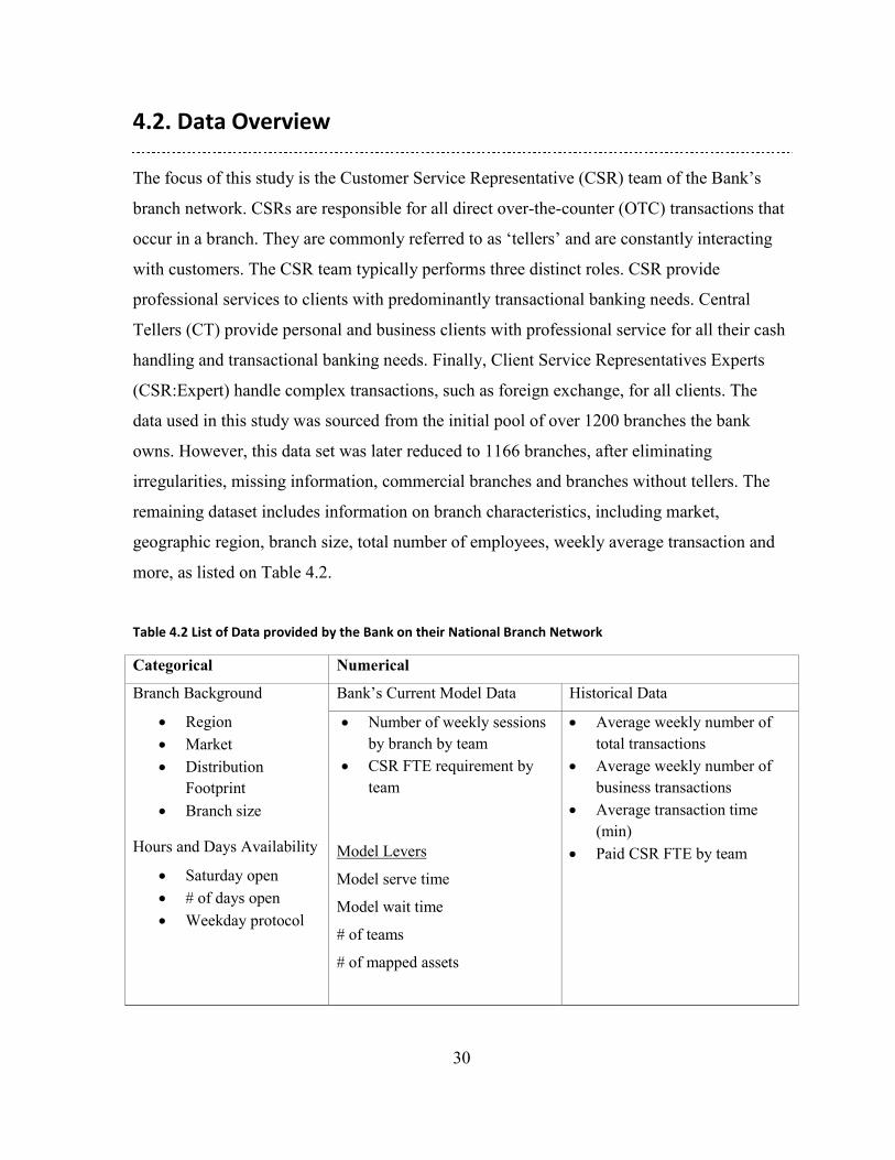
4.2. Data Overview
The focus of this study is the Customer Service Representative (CSR) team of the Bank’s
branch network. CSRs are responsible for all direct over-the-counter (OTC) transactions that
occur in a branch. They are commonly referred to as ‘tellers’ and are constantly interacting
with customers. The CSR team typically performs three distinct roles. CSR provide
professional services to clients with predominantly transactional banking needs. Central
Tellers (CT) provide personal and business clients with professional service for all their cash
handling and transactional banking needs. Finally, Client Service Representatives Experts
(CSR:Expert) handle complex transactions, such as foreign exchange, for all clients. The
data used in this study was sourced from the initial pool of over 1200 branches the bank
owns. However, this data set was later reduced to 1166 branches, after eliminating
irregularities, missing information, commercial branches and branches without tellers. The
remaining dataset includes information on branch characteristics, including market,
geographic region, branch size, total number of employees, weekly average transaction and
more, as listed on Table 4.2.
Table 4.2 List of Data provided by the Bank on their National Branch Network
Categorical Numerical
Branch Background
• Region • Market • Distribution
Footprint • Branch size
Hours and Days Availability
• Saturday open • # of days open • Weekday protocol
Bank’s Current Model Data Historical Data
• Number of weekly sessions by branch by team
• CSR FTE requirement by team
Model Levers
Model serve time
Model wait time
# of teams
# of mapped assets
• Average weekly number of total transactions
• Average weekly number of business transactions
• Average transaction time (min)
• Paid CSR FTE by team
31
4.3 The Bank’s Current Staff Allocation Model (BCM) Overview
This section provides an overview of the BCM including the overall managerial decision
making process and the performance ratios used by the Bank.
4.3.1 Definitions
A Transaction Time starts when a client approaches the counter and swipes their card to
initiate a transaction and ends when the transaction finishes as the account is closed by the
teller in the system. Such a method of collecting transaction times may incur some potential
errors if an employee forgets to close the account in between transactions.
Full Time Equivalent (FTE) represents one full time employee’s base hours of work in a
week, which is 37.5 hours/week. In this study, FTE is used to measure the amount of human
resource units needed for branch operations.
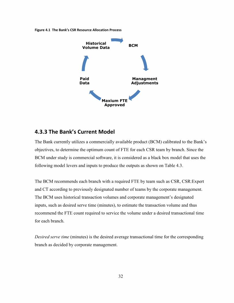
4.3.2 CSR Resource Allocation Process
The CSR resource allocation process involves a complex model as well as management’s
input to prescribe appropriate resource deployment to each branch. Such a process is a cycle
where the Bank’s model uses historical transaction volume data and other model levers to
estimate the optimum FTE per branch by team, which then goes under management’s
adjustments to add in other factors, such as coverage, to determine the Net FTE by branch.
Such Net FTE is then used to determine the final maximum number of approved FTEs per
branch and this cycle completes when the actual paid FTE data (Paid Data) enters their
internal data server with other information including transaction time and number of
transactions. As shown in Figure 4.1, it completes the cycle as the model uses the updated
historical data to re-calculate the optimum resource distribution for the next season.
32
Figure 4.1 The Bank’s CSR Resource Allocation Process
4.3.3 The Bank’s Current Model
The Bank currently utilizes a commercially available product (BCM) calibrated to the Bank’s
objectives, to determine the optimum count of FTE for each CSR team by branch. Since the
BCM under study is commercial software, it is considered as a black box model that uses the
following model levers and inputs to produce the outputs as shown on Table 4.3.
The BCM recommends each branch with a required FTE by team such as CSR, CSR:Expert
and CT according to previously designated number of teams by the corporate management.
The BCM uses historical transaction volumes and corporate management’s designated
inputs, such as desired serve time (minutes), to estimate the transaction volume and thus
recommend the FTE count required to service the volume under a desired transactional time
for each branch.
Desired serve time (minutes) is the desired average transactional time for the corresponding
branch as decided by corporate management.
BCM
Managment Adjustments
Maxium FTE Approved
Paid Data
Historical Volume Data
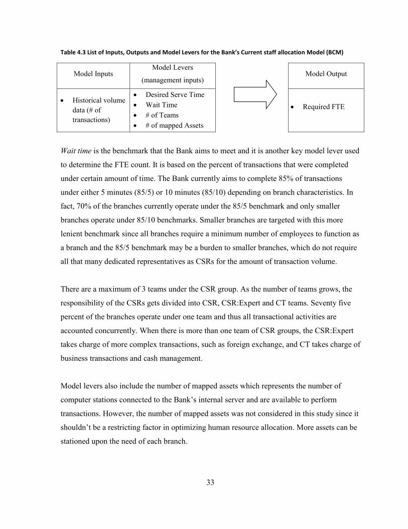
33
Table 4.3 List of Inputs, Outputs and Model Levers for the Bank’s Current staff allocation Model (BCM)
Model Inputs Model Levers
(management inputs)
Model Output
• Historical volume data (# of transactions)
• Desired Serve Time • Wait Time • # of Teams • # of mapped Assets
• Required FTE
Wait time is the benchmark that the Bank aims to meet and it is another key model lever used
to determine the FTE count. It is based on the percent of transactions that were completed
under certain amount of time. The Bank currently aims to complete 85% of transactions
under either 5 minutes (85/5) or 10 minutes (85/10) depending on branch characteristics. In
fact, 70% of the branches currently operate under the 85/5 benchmark and only smaller
branches operate under 85/10 benchmarks. Smaller branches are targeted with this more
lenient benchmark since all branches require a minimum number of employees to function as
a branch and the 85/5 benchmark may be a burden to smaller branches, which do not require
all that many dedicated representatives as CSRs for the amount of transaction volume.
There are a maximum of 3 teams under the CSR group. As the number of teams grows, the
responsibility of the CSRs gets divided into CSR, CSR:Expert and CT teams. Seventy five
percent of the branches operate under one team and thus all transactional activities are
accounted concurrently. When there is more than one team of CSR groups, the CSR:Expert
takes charge of more complex transactions, such as foreign exchange, and CT takes charge of
business transactions and cash management.
Model levers also include the number of mapped assets which represents the number of
computer stations connected to the Bank’s internal server and are available to perform
transactions. However, the number of mapped assets was not considered in this study since it
shouldn’t be a restricting factor in optimizing human resource allocation. More assets can be
stationed upon the need of each branch.
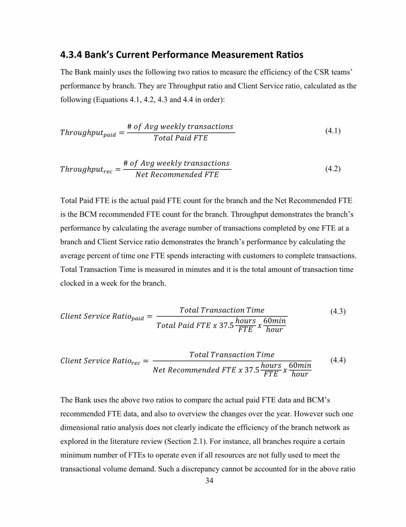
34
4.3.4 Bank’s Current Performance Measurement Ratios
The Bank mainly uses the following two ratios to measure the efficiency of the CSR teams’
performance by branch. They are Throughput ratio and Client Service ratio, calculated as the
following (Equations 4.1, 4.2, 4.3 and 4.4 in order):
}~��/m~?/�"�@� �������3m�J�������������������
}�����������}�
}~��/m~?/�D�� �������3m�J�������������������
�����������������}�
Total Paid FTE is the actual paid FTE count for the branch and the Net Recommended FTE
is the BCM recommended FTE count for the branch. Throughput demonstrates the branch’s
performance by calculating the average number of transactions completed by one FTE at a
branch and Client Service ratio demonstrates the branch’s performance by calculating the
average percent of time one FTE spends interacting with customers to complete transactions.
Total Transaction Time is measured in minutes and it is the total amount of transaction time
clocked in a week for the branch.
����������3���������"�@� ��}�����}�����������}���
}�����������}�������� ~�/���}� � �:���~�/� �
����������3���������D�� ��}�����}�����������}���
�����������������}�������� ~�/���}� � �:���~�/�
The Bank uses the above two ratios to compare the actual paid FTE data and BCM’
recommended FTE data, and also to overview the changes over the year. However s
dimensional ratio analysis does not clearly indicate the efficiency of the branch netw
explored in the literature review (Section 2.1). For instance, all branches require a c
minimum number of FTEs to operate even if all resources are not fully used to mee
transactional volume demand. Such a discrepancy cannot be accounted for in the ab
(4.4)
(4.3)
(4.2)
(4.1)
s
uch one
ork as
ertain
t the
ove ratio
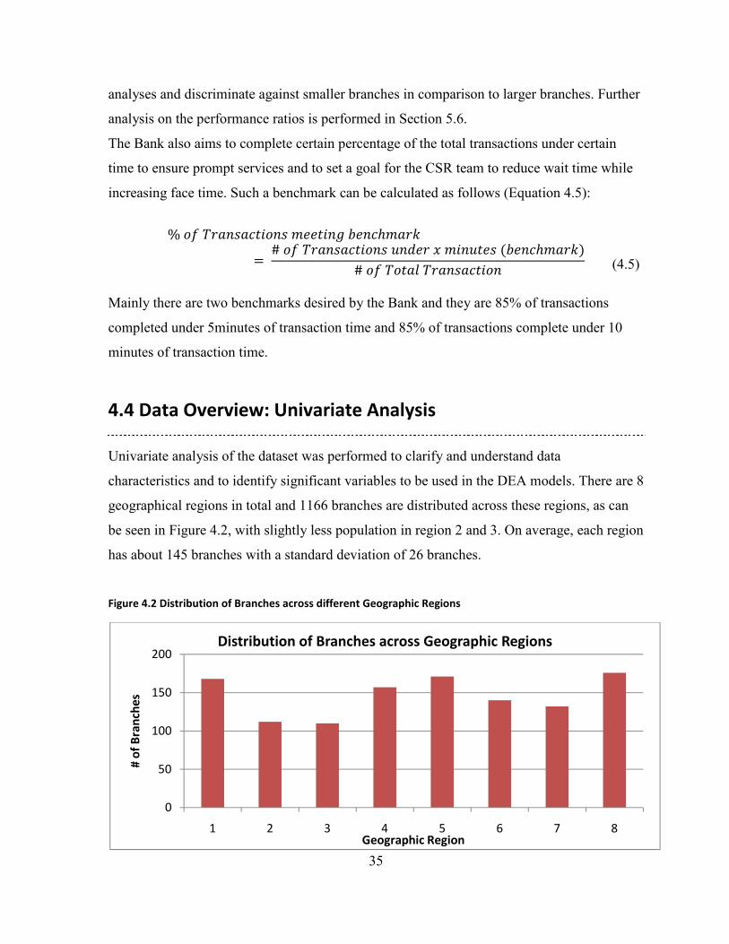
35
analyses and discriminate against smaller branches in comparison to larger branches. Further
analysis on the performance ratios is performed in Section 5.6.
The Bank also aims to complete certain percentage of the total transactions under certain
time to ensure prompt services and to set a goal for the CSR team to reduce wait time while
increasing face time. Such a benchmark can be calculated as follows (Equation 4.5):
�����}������������������m�����~����
� ������}������������/����������/���������~����������}�����}����������
Mainly there are two benchmarks desired by the Bank and they are 85% of transactions
completed under 5minutes of transaction time and 85% of transactions complete under
minutes of transaction time.
4.4 Data Overview: Univariate Analysis
Univariate analysis of the dataset was performed to clarify and understand data
characteristics and to identify significant variables to be used in the DEA models. Ther
geographical regions in total and 1166 branches are distributed across these regions, as
be seen in Figure 4.2, with slightly less population in region 2 and 3. On average, each
has about 145 branches with a standard deviation of 26 branches.
Figure 4.2 Distribution of Branches across different Geographic Regions
0
50
100
150
200
1 2 3 4 5 6 7
# of
Bra
nche
s
Geographic Region
Distribution of Branches across Geographic Regions
(4.5)
10
e are 8
can
region
8
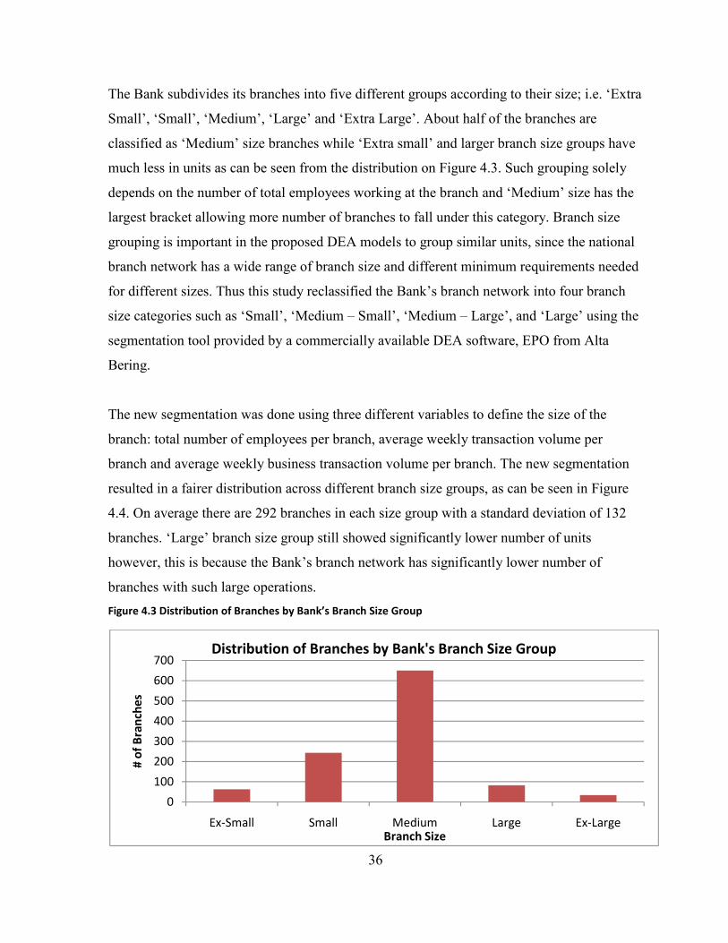
36
The Bank subdivides its branches into five different groups according to their size; i.e. ‘Extra
Small’, ‘Small’, ‘Medium’, ‘Large’ and ‘Extra Large’. About half of the branches are
classified as ‘Medium’ size branches while ‘Extra small’ and larger branch size groups have
much less in units as can be seen from the distribution on Figure 4.3. Such grouping solely
depends on the number of total employees working at the branch and ‘Medium’ size has the
largest bracket allowing more number of branches to fall under this category. Branch size
grouping is important in the proposed DEA models to group similar units, since the national
branch network has a wide range of branch size and different minimum requirements needed
for different sizes. Thus this study reclassified the Bank’s branch network into four branch
size categories such as ‘Small’, ‘Medium – Small’, ‘Medium – Large’, and ‘Large’ using the
segmentation tool provided by a commercially available DEA software, EPO from Alta
Bering.
The new segmentation was done using three different variables to define the size of the
branch: total number of employees per branch, average weekly transaction volume per
branch and average weekly business transaction volume per branch. The new segmentation
resulted in a fairer distribution across different branch size groups, as can be seen in Figure
4.4. On average there are 292 branches in each size group with a standard deviation of 132
branches. ‘Large’ branch size group still showed significantly lower number of units
however, this is because the Bank’s branch network has significantly lower number of
branches with such large operations.
Figure 4.3 Distribution of Branches by Bank’s Branch Size Group
0
100
200
300
400
500
600
700
Ex-Small Small Medium Large Ex-Large
# of
Bra
nche
s
Branch Size
Distribution of Branches by Bank's Branch Size Group
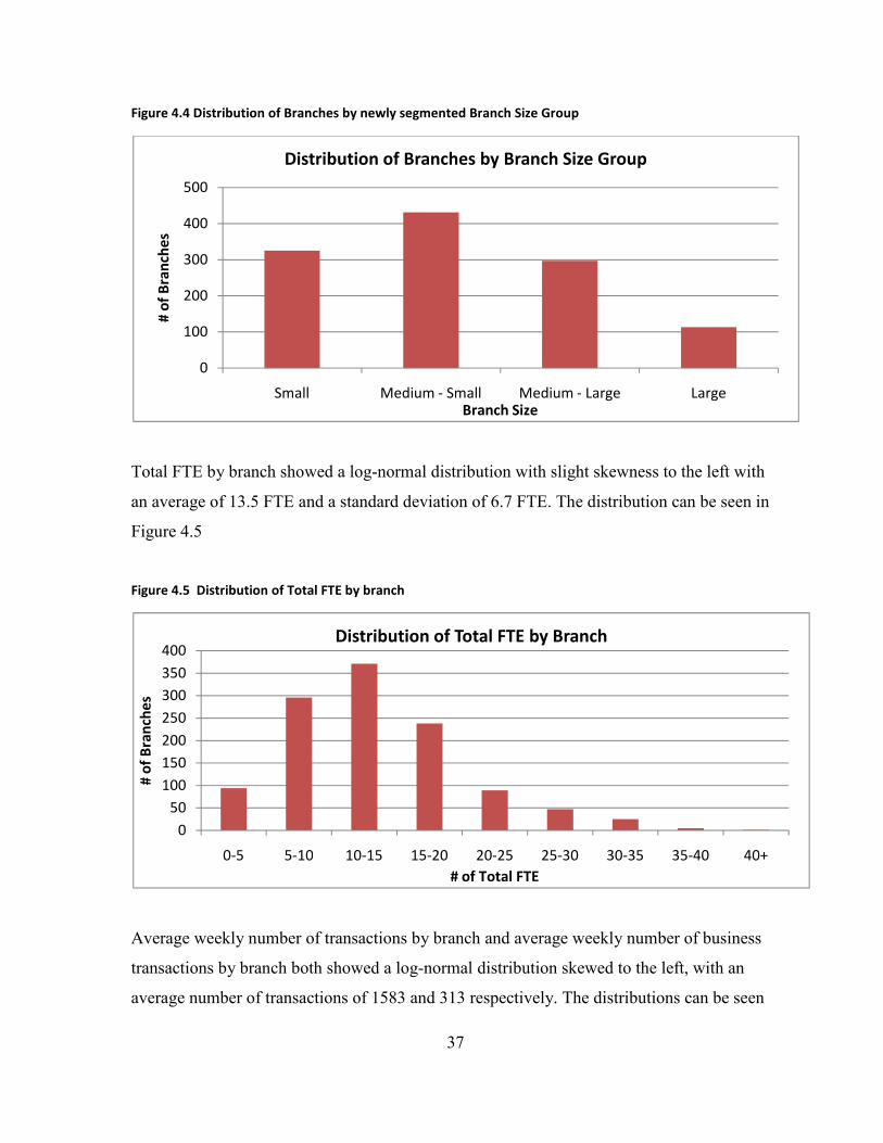
37
Figure 4.4 Distribution of Branches by newly segmented Branch Size Group
Total FTE by branch showed a log-normal distribution with slight skewness to the left with
an average of 13.5 FTE and a standard deviation of 6.7 FTE. The distribution can be seen in
Figure 4.5
Figure 4.5 Distribution of Total FTE by branch
Average weekly number of transactions by branch and average weekly number of business
transactions by branch both showed a log-normal distribution skewed to the left, with an
average number of transactions of 1583 and 313 respectively. The distributions can be seen
0
100
200
300
400
500
Small Medium - Small Medium - Large Large
# of
Bra
nche
s
Branch Size
Distribution of Branches by Branch Size Group
050
100150200250300350400
0-5 5-10 10-15 15-20 20-25 25-30 30-35 35-40 40+
# of
Bra
nche
s
# of Total FTE
Distribution of Total FTE by Branch
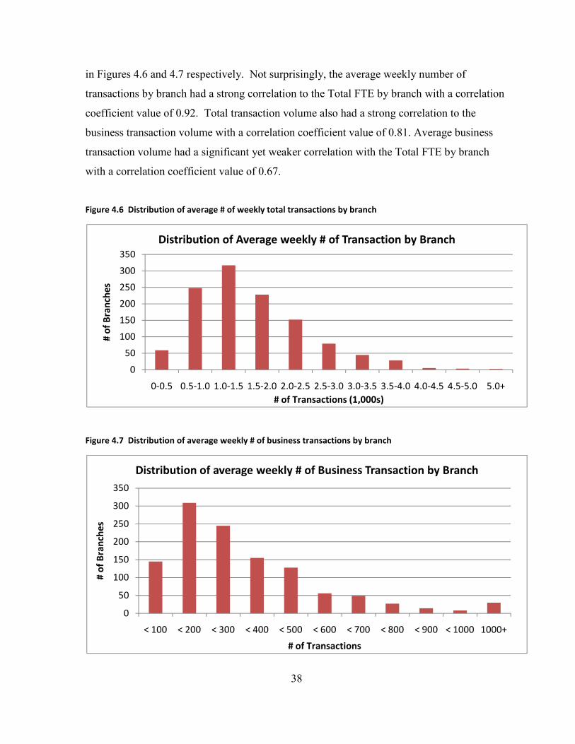
38
in Figures 4.6 and 4.7 respectively. Not surprisingly, the average weekly number of
transactions by branch had a strong correlation to the Total FTE by branch with a correlation
coefficient value of 0.92. Total transaction volume also had a strong correlation to the
business transaction volume with a correlation coefficient value of 0.81. Average business
transaction volume had a significant yet weaker correlation with the Total FTE by branch
with a correlation coefficient value of 0.67.
Figure 4.6 Distribution of average # of weekly total transactions by branch
Figure 4.7 Distribution of average weekly # of business transactions by branch
0
50
100
150
200
250
300
350
0-0.5 0.5-1.0 1.0-1.5 1.5-2.0 2.0-2.5 2.5-3.0 3.0-3.5 3.5-4.0 4.0-4.5 4.5-5.0 5.0+
# of
Bra
nche
s
# of Transactions (1,000s)
Distribution of Average weekly # of Transaction by Branch
0
50
100
150
200
250
300
350
< 100 < 200 < 300 < 400 < 500 < 600 < 700 < 800 < 900 < 1000 1000+
# of
Bra
nche
s
# of Transactions
Distribution of average weekly # of Business Transaction by Branch
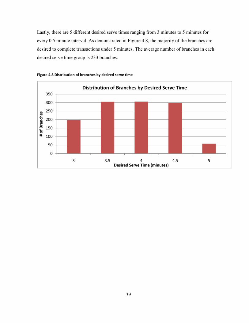
39
Lastly, there are 5 different desired serve times ranging from 3 minutes to 5 minutes for
every 0.5 minute interval. As demonstrated in Figure 4.8, the majority of the branches are
desired to complete transactions under 5 minutes. The average number of branches in each
desired serve time group is 233 branches.
Figure 4.8 Distribution of branches by desired serve time
0
50
100
150
200
250
300
350
3 3.5 4 4.5 5
# of
Bra
nche
s
Desired Serve Time (minutes)
Distribution of Branches by Desired Serve Time
40
CHAPTER 5:
DEA MODEL #1 FORMULATION AND RESULTS: EVALUATING BCM’S PERFORMANCE This chapter provides an overview of the Data Envelopment Analysis (DEA) model
proposed to evaluate the staff allocating model of the Bank under study. The Bank uses a
black box model (BCM) that corporate management uses to allocate the required FTE for the
CSR teams across their national branch network. In this study, DEA is used to develop an
evaluation system to validate the staffing allocation across the Bank’s branch network and to
evaluate the performance of the model and the branches. To evaluate the BCM, this chapter
constructed a DEA model to best represent the network of resources and their relationship to
the outputs. The input oriented DEA model was employed since inputs are much more
controllable than the outputs in the given industry setting.
This section discusses the concepts and definitions of the proposed DEA models; i.e. the
inputs, outputs and non-controllable variables used. Furthermore, a summary of the results of
the DEA analysis is provided with information including the CRS and VRS scores, as well as
the results of the local geographical and branch size comparisons.
5.1 Data Employed
The focus of this study is on the evaluation of managing CSR allocations across the Bank’s
branch network. The Bank under study provided the data for this study. After eliminating
large commercial, teller-less branches as well as missing information and irregularities, the
total number of branches under study was reduced from over 1200 to 1166. Branch
information is further subdivided into four major branch size groups: ‘Small’, ‘Medium-
Small’, ‘Medium-Large’ and ‘Large’ according to three variables that could classify a
branch’s size (Section 4.4).
41
5.2 Model Formulation: Evaluating the BCM’s performance
The goal of this DEA model is to examine the efficiency of the BCM by looking at staff
efficiency and allocation of FTEs for the corresponding CSR teams, so that the branch would
be able to complete the same volume of transactions with fewer FTEs than before. Therefore,
an input oriented model was employed to reduce the number of FTEs to produce the same
volume of transactions.
An important step in the efficiency analysis lies with defining the input and output variables.
The inputs of this DEA model consisted of BCM’s recommended FTE count by team (CSR,
CSR:Expert, CT) and the outputs of this model consisted of the average weekly number of
personal client transactions calculated over the year and the average weekly number of
business client transactions calculated over the year (two values that define the demand for
branch work throughout the year). There are other variables that also affect the use of branch
resources and they are branch size, desired serve time, wait time, and number of teams.
These variables were included in the model as non-controllable inputs since, although they
have an effect in the use of resources and producing transactions, they are not controllable by
the bank, hence, cannot be included in the BCM. The following describes the non-
controllable inputs used in the model in detail:
• Branch Size: the total number of employees at the branch varied quite widely; hence,
it was essential to differentiate the branches in terms of their size, so that each branch
would only be compared against those similar to it.
• Desired Serve Time: the desired serve time ranged from 3 to 5 minutes and it is
designated by the corporate management for each branch as to what the desired
average transaction time is and thus would affect the staffing of each branch.
• Wait Time: the wait time is the benchmark of meeting 85% transactions under a
certain amount of minutes where this varied from 5 minutes to 10 minutes and the
difference between two benchmarks would result in higher staffing for the 85/5
benchmarked branch.
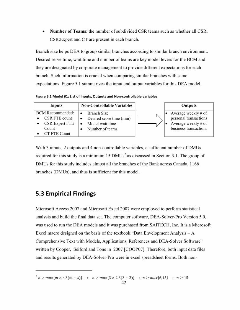
42
• Number of Teams: the number of subdivided CSR teams such as whether all CSR,
CSR:Expert and CT are present in each branch.
Branch size helps DEA to group similar branches according to similar branch environment.
Desired serve time, wait time and number of teams are key model levers for the BCM and
they are designated by corporate management to provide different expectations for each
branch. Such information is crucial when comparing similar branches with same
expectations. Figure 5.1 summarizes the input and output variables for this DEA model.
Figure 5.1 Model #1: List of Inputs, Outputs and Non-controllable variables
Inputs Non-Controllable Variables
Outputs
BCM Recommended: • CSR FTE count • CSR:Expert FTE
Count • CT FTE Count
• Branch Size • Desired serve time (min) • Model wait time • Number of teams
• Average weekly # of personal transactions
• Average weekly # of business transactions
With 3 inputs, 2 outputs and 4 non-controllable variables, a sufficient number of DMUs
required for this study is a minimum 15 DMUs2 as discussed in Section 3.1. The group of
DMUs for this study includes almost all the branches of the Bank across Canada, 1166
branches (DMUs), and thus is sufficient for this model.
5.3 Empirical Findings
Microsoft Access 2007 and Microsoft Excel 2007 were employed to perform statistical
analysis and build the final data set. The computer software, DEA-Solver-Pro Version 5.0,
was used to run the DEA models and it was purchased from SAITECH, Inc. It is a Microsoft
Excel macro designed on the basis of the textbook “Data Envelopment Analysis – A
Comprehensive Text with Models, Applications, References and DEA-Solver Software”
written by Cooper, Seiford and Tone in 2007 [COOP07]. Therefore, both input data files
and results generated by DEA-Solver-Pro were in excel spreadsheet forms. Both non-
2 � � ����� � ���� ��� → � � ����� � ���� ��� → �� � �����7����→ ��� � 7�
43
controllable CRS Input oriented “NCN-C-I” and non-controllable VRS Input oriented
“NCN-V-I” were used in this study.
A three-part analysis was performed on the result. In the first part, a CRS input oriented
DEA model, as well as the VRS input oriented DEA model, were employed to evaluate the
efficiency of the entire sample of the bank branches. In the second part, both CRS and VRS
input oriented results were grouped by branch size to explore the performance differences
between different branch size groups. In the third part, both CRS and VRS input oriented
model results were grouped by geographical regions to explore significant regional
differences observed from the model.
5.3.1 Model #1: Result for All Branches
In the first run, CRS and VRS input oriented DEA models were used to calculate the relative
efficiencies of the 1166 branches across Canada. 154 branches were found to be CRS
efficient (efficiency =1) and 174 branches were found to be VRS efficient; i.e. approximately
15% of the network were discovered to be DEA efficient. The overall average of the CRS
efficiency was 72.4% with a standard deviation of 20.7% and the VRS efficiency showed a
similar result and displayed 73.4% average efficiency score with a standard deviation of
20.9%. Since the ratio of the CRS and the VRS efficiency score is close to 1(Scale
Efficiency), one can conclude that the Bank’s process is actually a natural CRS process
[TOCH06]. The summary of CRS and VRS results for all branches, as well as the frequency
distribution of the two models, are presented in Table 5.1 and Figure 5.2 respectively.
As expected from one of the large banks in Canada, the distribution of the efficiency score is
skewed to the right with significant cluster of branches with efficiency score of 1.0. It is
important to note that the DEA still was able to distinguish high performing branches from
the inefficient branches as the efficiency score ranged from 18% to the fully efficient, 100%.
The branches that are in the lower bracket of the efficiency distribution should be reviewed
by management to reveal sources of potential improvement in resource allocation.
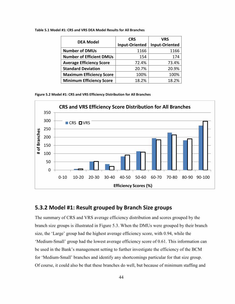
44
Table 5.1 Model #1: CRS and VRS DEA Model Results for All Branches
DEA Model CRS
Input-Oriented VRS
Input-Oriented Number of DMUs 1166 1166 Number of Efficient DMUs 154 174 Average Efficiency Score 72.4% 73.4% Standard Deviation 20.7% 20.9% Maximum Efficiency Score 100% 100% Minimum Efficiency Score 18.2% 18.2%
Figure 5.2 Model #1: CRS and VRS Efficiency Distribution for All Branches
5.3.2 Model #1: Result grouped by Branch Size groups
The summary of CRS and VRS average efficiency distribution and scores grouped by the
branch size groups is illustrated in Figure 5.3. When the DMUs were grouped by their branch
size, the ‘Large’ group had the highest average efficiency score, with 0.94, while the
‘Medium-Small’ group had the lowest average efficiency score of 0.61. This information can
be used in the Bank’s management setting to further investigate the efficiency of the BCM
for ‘Medium-Small’ branches and identify any shortcomings particular for that size group.
Of course, it could also be that these branches do well, but because of minimum staffing and
0
50
100
150
200
250
300
350
0-10 10-20 20-30 30-40 40-50 50-60 60-70 70-80 80-90 90-100
# of
Bra
nche
s
Efficiency Scores (%)
CRS and VRS Efficiency Score Distribution for All Branches
CRS VRS
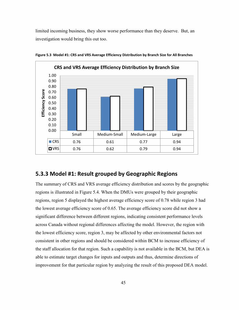
45
limited incoming business, they show worse performance than they deserve. But, an
investigation would bring this out too.
Figure 5.3 Model #1: CRS and VRS Average Efficiency Distribution by Branch Size for All Branches
5.3.3 Model #1: Result grouped by Geographic Regions
The summary of CRS and VRS average efficiency distribution and scores by the geographic
regions is illustrated in Figure 5.4. When the DMUs were grouped by their geographic
regions, region 5 displayed the highest average efficiency score of 0.78 while region 3 had
the lowest average efficiency score of 0.65. The average efficiency score did not show a
significant difference between different regions, indicating consistent performance levels
across Canada without regional differences affecting the model. However, the region with
the lowest efficiency score, region 3, may be affected by other environmental factors not
consistent in other regions and should be considered within BCM to increase efficiency of
the staff allocation for that region. Such a capability is not available in the BCM, but DEA is
able to estimate target changes for inputs and outputs and thus, determine directions of
improvement for that particular region by analyzing the result of this proposed DEA model.
Small Medium-Small Medium-Large Large
CRS 0.76 0.61 0.77 0.94
VRS 0.76 0.62 0.79 0.94
0.000.100.200.300.400.500.600.700.800.901.00
Effic
ienc
y Sc
ore
CRS and VRS Average Efficiency Distribution by Branch Size

46
Figure 5.4 Model #1: CRS and VRS Average Efficiency Distribution by Geographic Region for All Branches
5.3.4 Comparison between Paid FTE and BCM Recommended FTE
Building on the previous DEA model, another model based on the actual paid FTE value was
built to measure the potential efficiency gain by the BCM recommendation when compared
to the actual FTE input that was used to produce the number of transactions in the historical
data. For this model, actual paid FTE counts by CSR team (CSR, CT, CSR:Expert) were
used as input variables, so that the corresponding DEA result can be compared with the BCM
recommended DEA result (Model #1).
Figure 5.5 Actual Paid Model: List of Inputs, Outputs and Non-controllable variables
Inputs Non-Controllable
Variables
Outputs
Actual paid FTE count:
• CSR • CSR:Expert • CT
• Branch Size • Model desired serve
Time (min) • Model wait time • # of teams
• Average weekly # of personal transactions
• Average weekly # of business transactions
1 2 3 4 5 6 7 8
CRS 0.71 0.71 0.65 0.77 0.78 0.71 0.70 0.74
VRS 0.72 0.75 0.66 0.77 0.79 0.72 0.71 0.74
0.00
0.10
0.20
0.30
0.40
0.50
0.60
0.70
0.80
0.90
Effic
ienc
y Sc
ore
CRS and VRS Average Efficiency Distribution by Geographic Region
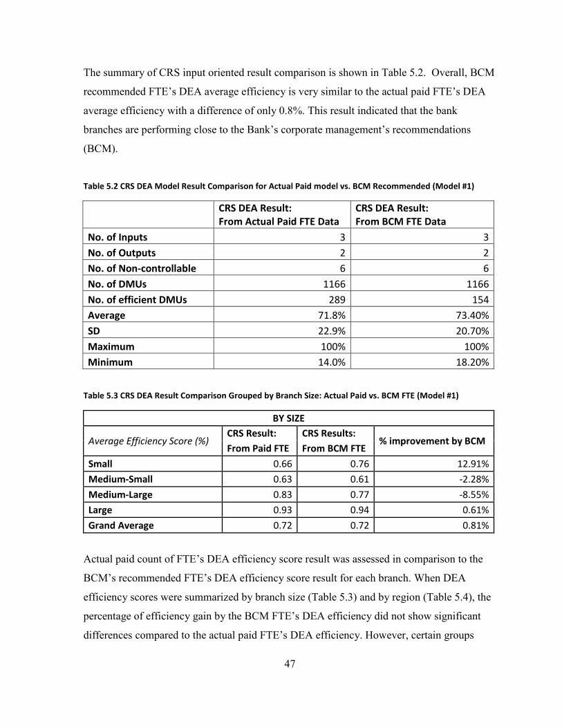
47
The summary of CRS input oriented result comparison is shown in Table 5.2. Overall, BCM
recommended FTE’s DEA average efficiency is very similar to the actual paid FTE’s DEA
average efficiency with a difference of only 0.8%. This result indicated that the bank
branches are performing close to the Bank’s corporate management’s recommendations
(BCM).
Table 5.2 CRS DEA Model Result Comparison for Actual Paid model vs. BCM Recommended (Model #1)
CRS DEA Result: From Actual Paid FTE Data
CRS DEA Result: From BCM FTE Data
No. of Inputs 3 3 No. of Outputs 2 2 No. of Non-controllable 6 6 No. of DMUs 1166 1166 No. of efficient DMUs 289 154 Average 71.8% 73.40% SD 22.9% 20.70% Maximum 100% 100% Minimum 14.0% 18.20%
Table 5.3 CRS DEA Result Comparison Grouped by Branch Size: Actual Paid vs. BCM FTE (Model #1)
BY SIZE
Average Efficiency Score (%) CRS Result: CRS Results:
% improvement by BCM From Paid FTE From BCM FTE
Small 0.66 0.76 12.91%
Medium-Small 0.63 0.61 -2.28%
Medium-Large 0.83 0.77 -8.55%
Large 0.93 0.94 0.61%
Grand Average 0.72 0.72 0.81%
Actual paid count of FTE’s DEA efficiency score result was assessed in comparison to the
BCM’s recommended FTE’s DEA efficiency score result for each branch. When DEA
efficiency scores were summarized by branch size (Table 5.3) and by region (Table 5.4), the
percentage of efficiency gain by the BCM FTE’s DEA efficiency did not show significant
differences compared to the actual paid FTE’s DEA efficiency. However, certain groups
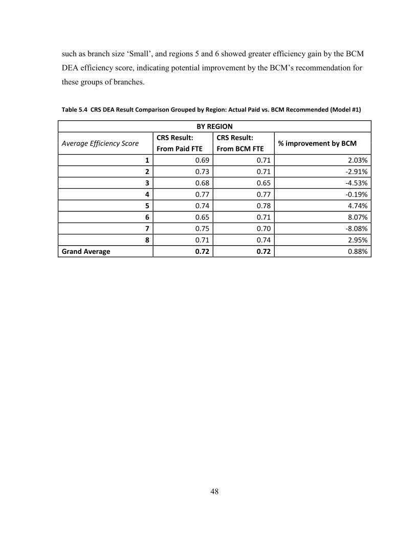
48
such as branch size ‘Small’, and regions 5 and 6 showed greater efficiency gain by the BCM
DEA efficiency score, indicating potential improvement by the BCM’s recommendation for
these groups of branches.
Table 5.4 CRS DEA Result Comparison Grouped by Region: Actual Paid vs. BCM Recommended (Model #1)
BY REGION
Average Efficiency Score CRS Result: CRS Result:
% improvement by BCM From Paid FTE From BCM FTE
1 0.69 0.71 2.03%
2 0.73 0.71 -2.91%
3 0.68 0.65 -4.53%
4 0.77 0.77 -0.19%
5 0.74 0.78 4.74%
6 0.65 0.71 8.07%
7 0.75 0.70 -8.08%
8 0.71 0.74 2.95%
Grand Average 0.72 0.72 0.88%
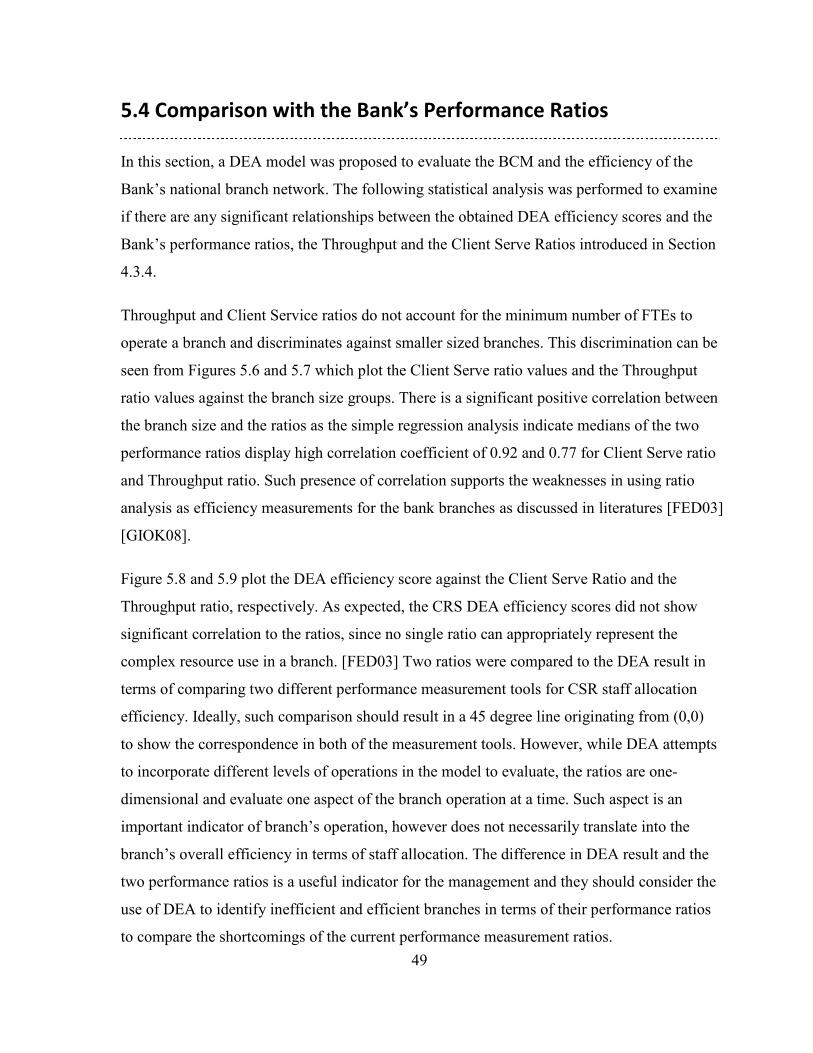
49
5.4 Comparison with the Bank’s Performance Ratios
In this section, a DEA model was proposed to evaluate the BCM and the efficiency of the
Bank’s national branch network. The following statistical analysis was performed to examine
if there are any significant relationships between the obtained DEA efficiency scores and the
Bank’s performance ratios, the Throughput and the Client Serve Ratios introduced in Section
4.3.4.
Throughput and Client Service ratios do not account for the minimum number of FTEs to
operate a branch and discriminates against smaller sized branches. This discrimination can be
seen from Figures 5.6 and 5.7 which plot the Client Serve ratio values and the Throughput
ratio values against the branch size groups. There is a significant positive correlation between
the branch size and the ratios as the simple regression analysis indicate medians of the two
performance ratios display high correlation coefficient of 0.92 and 0.77 for Client Serve ratio
and Throughput ratio. Such presence of correlation supports the weaknesses in using ratio
analysis as efficiency measurements for the bank branches as discussed in literatures [FED03]
[GIOK08].
Figure 5.8 and 5.9 plot the DEA efficiency score against the Client Serve Ratio and the
Throughput ratio, respectively. As expected, the CRS DEA efficiency scores did not show
significant correlation to the ratios, since no single ratio can appropriately represent the
complex resource use in a branch. [FED03] Two ratios were compared to the DEA result in
terms of comparing two different performance measurement tools for CSR staff allocation
efficiency. Ideally, such comparison should result in a 45 degree line originating from (0,0)
to show the correspondence in both of the measurement tools. However, while DEA attempts
to incorporate different levels of operations in the model to evaluate, the ratios are one-
dimensional and evaluate one aspect of the branch operation at a time. Such aspect is an
important indicator of branch’s operation, however does not necessarily translate into the
branch’s overall efficiency in terms of staff allocation. The difference in DEA result and the
two performance ratios is a useful indicator for the management and they should consider the
use of DEA to identify inefficient and efficient branches in terms of their performance ratios
to compare the shortcomings of the current performance measurement ratios.
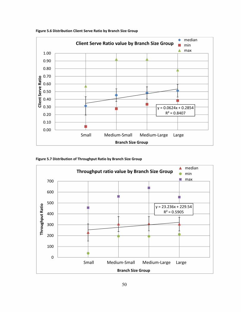
Figure 5.6 Distribution Client Serve Ratio by Branch Size Group
Figure 5.7 Distribution of Throughput Ratio by Branch Size Group
y = 0.0624x + 0.2854R² = 0.8407
0.00
0.10
0.20
0.30
0.40
0.50
0.60
0.70
0.80
0.90
1.00
0 1 2 3 4 5
Clie
nt S
erve
Rat
io
Branch Size Group
Client Serve Ratio value by Branch Size Groupmedianminmax
y = 23.236x + 229.54R² = 0.5905
0
100
200
300
400
500
600
700
Thro
ughp
ut R
atio
Throughput ratio value by Branch Size Groupmedianminmax
Small Medium-Small Medium-Large Large
Small Medium-Small Medium-Large Large
50
0 1 2 3 4 5Branch Size Group
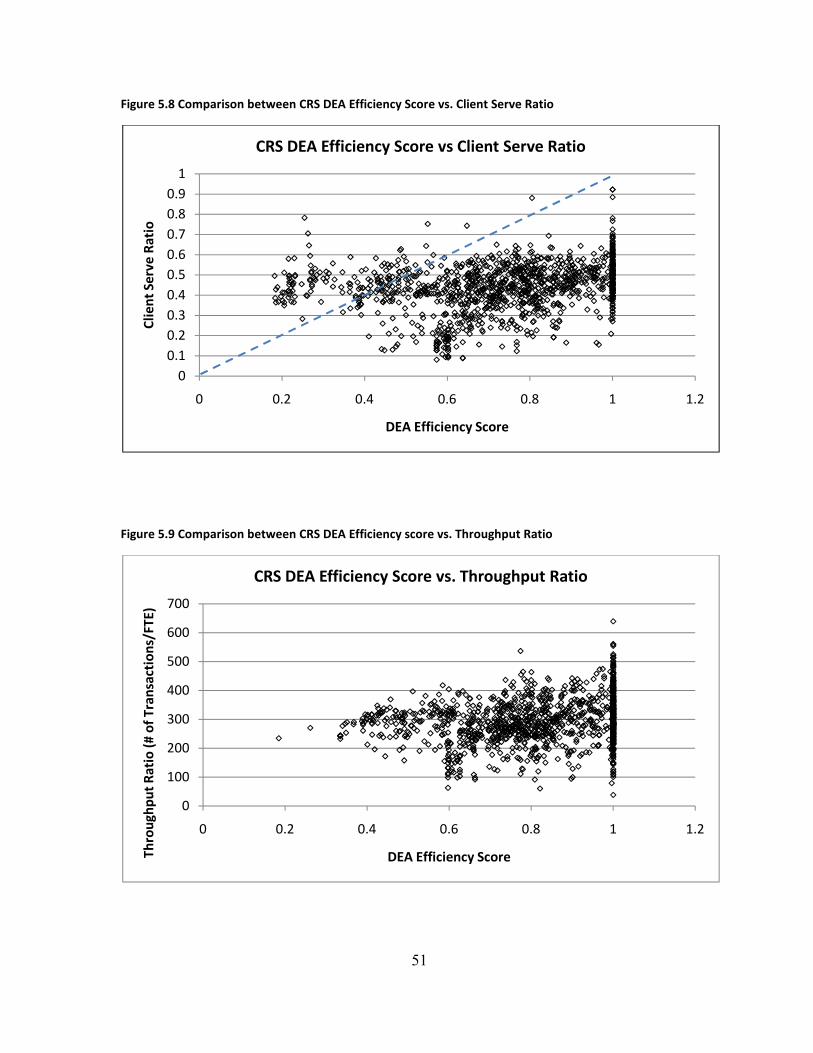
51
Figure 5.8 Comparison between CRS DEA Efficiency Score vs. Client Serve Ratio
Figure 5.9 Comparison between CRS DEA Efficiency score vs. Throughput Ratio
00.10.20.30.40.50.60.70.80.9
1
0 0.2 0.4 0.6 0.8 1 1.2
Clie
nt S
erve
Rat
io
DEA Efficiency Score
CRS DEA Efficiency Score vs Client Serve Ratio
0
100
200
300
400
500
600
700
0 0.2 0.4 0.6 0.8 1 1.2
Thro
ughp
ut R
atio
(# o
f Tra
nsac
tion
s/FT
E)
DEA Efficiency Score
CRS DEA Efficiency Score vs. Throughput Ratio
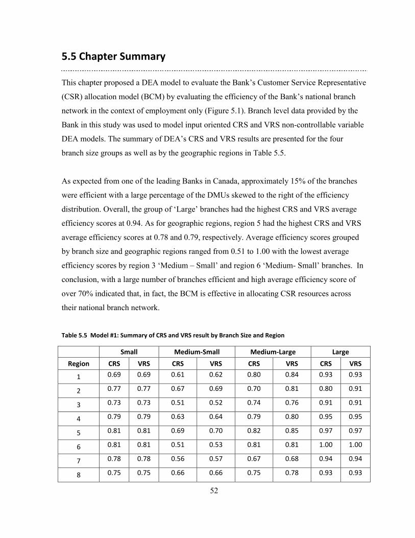
52
5.5 Chapter Summary
This chapter proposed a DEA model to evaluate the Bank’s Customer Service Representative
(CSR) allocation model (BCM) by evaluating the efficiency of the Bank’s national branch
network in the context of employment only (Figure 5.1). Branch level data provided by the
Bank in this study was used to model input oriented CRS and VRS non-controllable variable
DEA models. The summary of DEA’s CRS and VRS results are presented for the four
branch size groups as well as by the geographic regions in Table 5.5.
As expected from one of the leading Banks in Canada, approximately 15% of the branches
were efficient with a large percentage of the DMUs skewed to the right of the efficiency
distribution. Overall, the group of ‘Large’ branches had the highest CRS and VRS average
efficiency scores at 0.94. As for geographic regions, region 5 had the highest CRS and VRS
average efficiency scores at 0.78 and 0.79, respectively. Average efficiency scores grouped
by branch size and geographic regions ranged from 0.51 to 1.00 with the lowest average
efficiency scores by region 3 ‘Medium – Small’ and region 6 ‘Medium- Small’ branches. In
conclusion, with a large number of branches efficient and high average efficiency score of
over 70% indicated that, in fact, the BCM is effective in allocating CSR resources across
their national branch network.
Table 5.5 Model #1: Summary of CRS and VRS result by Branch Size and Region
Small Medium-Small Medium-Large Large
Region CRS VRS CRS VRS CRS VRS CRS VRS
1 0.69 0.69 0.61 0.62 0.80 0.84 0.93 0.93
2 0.77 0.77 0.67 0.69 0.70 0.81 0.80 0.91
3 0.73 0.73 0.51 0.52 0.74 0.76 0.91 0.91
4 0.79 0.79 0.63 0.64 0.79 0.80 0.95 0.95
5 0.81 0.81 0.69 0.70 0.82 0.85 0.97 0.97
6 0.81 0.81 0.51 0.53 0.81 0.81 1.00 1.00
7 0.78 0.78 0.56 0.57 0.67 0.68 0.94 0.94
8 0.75 0.75 0.66 0.66 0.75 0.78 0.93 0.93
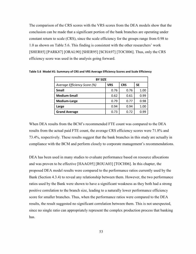
53
The comparison of the CRS scores with the VRS scores from the DEA models show that the
conclusion can be made that a significant portion of the bank branches are operating under
constant return to scale (CRS), since the scale efficiency for the groups range from 0.98 to
1.0 as shown on Table 5.6. This finding is consistent with the other researchers’ work
[SHER85] [PARK87] [ORAL90] [SHER95] [SCHA97] [TOCH06]. Thus, only the CRS
efficiency score was used in the analysis going forward.
Table 5.6 Model #1: Summary of CRS and VRS Average Efficiency Scores and Scale Efficiency
BY SIZE Average Efficiency Score (%) VRS CRS SE Small 0.76 0.76 1.00 Medium-Small 0.62 0.61 0.99 Medium-Large 0.79 0.77 0.98 Large 0.94 0.94 1.00 Grand Average 0.73 0.72 0.99
When DEA results from the BCM’s recommended FTE count was compared to the DEA
results from the actual paid FTE count, the average CRS efficiency scores were 71.8% and
73.4%, respectively. These results suggest that the bank branches in this study are actually in
compliance with the BCM and perform closely to corporate management’s recommendations.
DEA has been used in many studies to evaluate performance based on resource allocations
and was proven to be effective [HAAG95] [ROUA03] [TOCH06]. In this chapter, the
proposed DEA model results were compared to the performance ratios currently used by the
Bank (Section 4.3.4) to reveal any relationship between them. However, the two performance
ratios used by the Bank were shown to have a significant weakness as they both had a strong
positive correlation to the branch size, leading to a naturally lower performance efficiency
score for smaller branches. Thus, when the performance ratios were compared to the DEA
results, the result suggested no significant correlation between them. This is not unexpected,
since no single ratio can appropriately represent the complex production process that banking
has.
54
CHAPTER 6:
DEA MODEL #2 FORMULATION AND RESULTS: EVALUATING BCM’S ACCURACY This chapter provides an overview of the DEA model proposed to evaluate the accuracy of
the staff allocating model of the Bank under study in meeting the desired benchmarks set by
management. The BCM has a benchmark of meeting 85% of all transactions under either 5
or 10 minutes to reflect on customer satisfaction by promoting prompt services and reduced
wait times while increasing face time between the customer service representatives and
customers. In this chapter, DEA was employed to develop an evaluation system to validate or
deny BCM’s accuracy in meeting the desired benchmarks set by management.
This section discusses the concepts and definitions of the proposed DEA model, input
variables, output variables and non-controllable variables. Furthermore, a summary of the
results of the DEA analysis is provided with information including CRS scores as well as
comparisons with the Bank’s benchmarks.
6.1 Data Employed
The Bank under study provided detailed transactional data for 24 branches for a month of
either January, 2011 or May, 2011. Since the transaction volume over the year for a bank
branch does not experience any significant change throughout the year, two different month
data were used indifferently. After removing large commercial branches, this model
employed a dataset of all accounts of transactions over a one month period for 20 different
branches. The branch data was further broken down to an hourly average of transaction data
for each branch, increasing the size of the sample DMUs to 185.
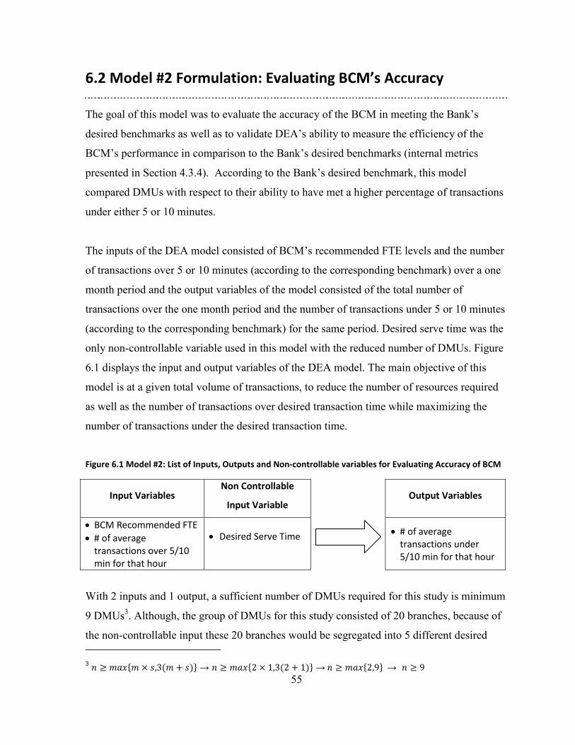
55
6.2 Model #2 Formulation: Evaluating BCM’s Accuracy
The goal of this model was to evaluate the accuracy of the BCM in meeting the Bank’s
desired benchmarks as well as to validate DEA’s ability to measure the efficiency of the
BCM’s performance in comparison to the Bank’s desired benchmarks (internal metrics
presented in Section 4.3.4). According to the Bank’s desired benchmark, this model
compared DMUs with respect to their ability to have met a higher percentage of transactions
under either 5 or 10 minutes.
The inputs of the DEA model consisted of BCM’s recommended FTE levels and the number
of transactions over 5 or 10 minutes (according to the corresponding benchmark) over a one
month period and the output variables of the model consisted of the total number of
transactions over the one month period and the number of transactions under 5 or 10 minutes
(according to the corresponding benchmark) for the same period. Desired serve time was the
only non-controllable variable used in this model with the reduced number of DMUs. Figure
6.1 displays the input and output variables of the DEA model. The main objective of this
model is at a given total volume of transactions, to reduce the number of resources required
as well as the number of transactions over desired transaction time while maximizing the
number of transactions under the desired transaction time.
Figure 6.1 Model #2: List of Inputs, Outputs and Non-controllable variables for Evaluating Accuracy of BCM
Input Variables Non Controllable
Input Variable Output Variables
• BCM Recommended FTE • # of average
transactions over 5/10 min for that hour
• Desired Serve Time • # of average transactions under 5/10 min for that hour
With 2 inputs and 1 output, a sufficient number of DMUs required for this study is minimum
9 DMUs3. Although, the group of DMUs for this study consisted of 20 branches, because of
the non-controllable input these 20 branches would be segregated into 5 different desired 3 � � ����� � ���� ��� → � � ����� � 7��� 7�� →�� � ���������→ � � �
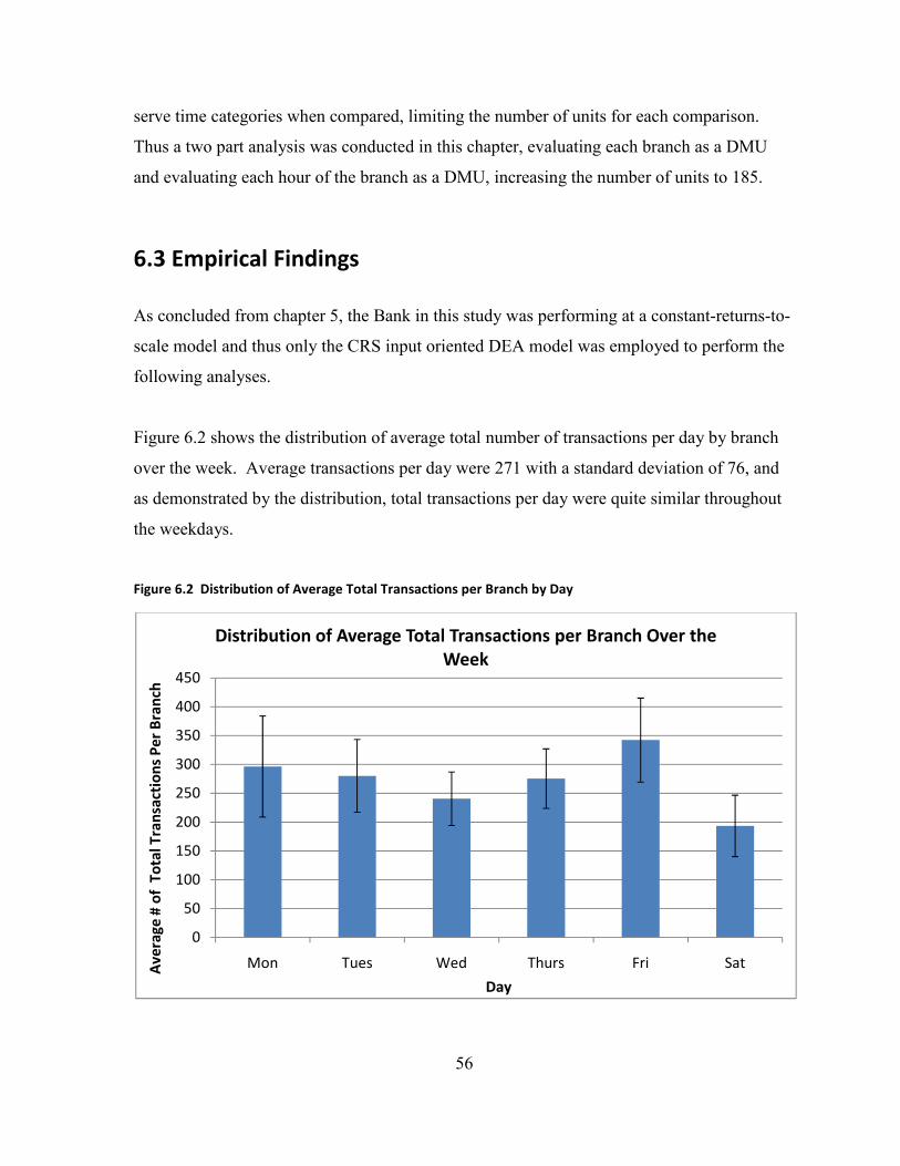
56
serve time categories when compared, limiting the number of units for each comparison.
Thus a two part analysis was conducted in this chapter, evaluating each branch as a DMU
and evaluating each hour of the branch as a DMU, increasing the number of units to 185.
6.3 Empirical Findings
As concluded from chapter 5, the Bank in this study was performing at a constant-returns-to-
scale model and thus only the CRS input oriented DEA model was employed to perform the
following analyses.
Figure 6.2 shows the distribution of average total number of transactions per day by branch
over the week. Average transactions per day were 271 with a standard deviation of 76, and
as demonstrated by the distribution, total transactions per day were quite similar throughout
the weekdays.
Figure 6.2 Distribution of Average Total Transactions per Branch by Day
0
50
100
150
200
250
300
350
400
450
Mon Tues Wed Thurs Fri SatAve
rage
# o
f To
tal T
rans
acti
ons
Per B
ranc
h
Day
Distribution of Average Total Transactions per Branch Over the Week
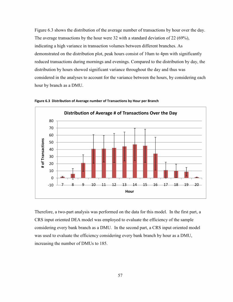
57
Figure 6.3 shows the distribution of the average number of transactions by hour over the day.
The average transactions by the hour were 32 with a standard deviation of 22 (69%),
indicating a high variance in transaction volumes between different branches. As
demonstrated on the distribution plot, peak hours consist of 10am to 4pm with significantly
reduced transactions during mornings and evenings. Compared to the distribution by day, the
distribution by hours showed significant variance throughout the day and thus was
considered in the analyses to account for the variance between the hours, by considering each
hour by branch as a DMU.
Figure 6.3 Distribution of Average number of Transactions by Hour per Branch
Therefore, a two-part analysis was performed on the data for this model. In the first part, a
CRS input oriented DEA model was employed to evaluate the efficiency of the sample
considering every bank branch as a DMU. In the second part, a CRS input oriented model
was used to evaluate the efficiency considering every bank branch by hour as a DMU,
increasing the number of DMUs to 185.
-10
0
10
20
30
40
50
60
70
80
7 8 9 10 11 12 13 14 15 16 17 18 19 20
# of
Tra
nsac
tion
s
Hour
Distribution of Average # of Transactions Over the Day
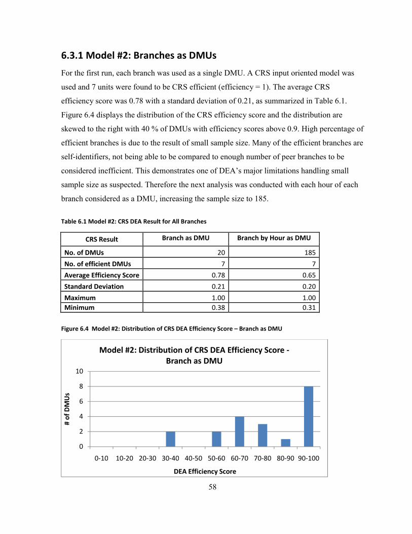
58
6.3.1 Model #2: Branches as DMUs
For the first run, each branch was used as a single DMU. A CRS input oriented model was
used and 7 units were found to be CRS efficient (efficiency = 1). The average CRS
efficiency score was 0.78 with a standard deviation of 0.21, as summarized in Table 6.1.
Figure 6.4 displays the distribution of the CRS efficiency score and the distribution are
skewed to the right with 40 % of DMUs with efficiency scores above 0.9. High percentage of
efficient branches is due to the result of small sample size. Many of the efficient branches are
self-identifiers, not being able to be compared to enough number of peer branches to be
considered inefficient. This demonstrates one of DEA’s major limitations handling small
sample size as suspected. Therefore the next analysis was conducted with each hour of each
branch considered as a DMU, increasing the sample size to 185.
Table 6.1 Model #2: CRS DEA Result for All Branches
CRS Result Branch as DMU Branch by Hour as DMU
No. of DMUs 20 185 No. of efficient DMUs 7 7 Average Efficiency Score 0.78 0.65 Standard Deviation 0.21 0.20 Maximum 1.00 1.00 Minimum 0.38 0.31
Figure 6.4 Model #2: Distribution of CRS DEA Efficiency Score – Branch as DMU
0
2
4
6
8
10
0-10 10-20 20-30 30-40 40-50 50-60 60-70 70-80 80-90 90-100
# of
DM
Us
DEA Efficiency Score
Model #2: Distribution of CRS DEA Efficiency Score -Branch as DMU
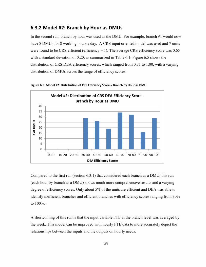
59
6.3.2 Model #2: Branch by Hour as DMUs
In the second run, branch by hour was used as the DMU. For example, branch #1 would now
have 8 DMUs for 8 working hours a day. A CRS input oriented model was used and 7 units
were found to be CRS efficient (efficiency = 1). The average CRS efficiency score was 0.65
with a standard deviation of 0.20, as summarized in Table 6.1. Figure 6.5 shows the
distribution of CRS DEA efficiency scores, which ranged from 0.31 to 1.00, with a varying
distribution of DMUs across the range of efficiency scores.
Figure 6.5 Model #2: Distribution of CRS Efficiency Score = Branch by Hour as DMU
Compared to the first run (section 6.3.1) that considered each branch as a DMU, this run
(each hour by branch as a DMU) shows much more comprehensive results and a varying
degree of efficiency scores. Only about 5% of the units are efficient and DEA was able to
identify inefficient branches and efficient branches with efficiency scores ranging from 30%
to 100%.
A shortcoming of this run is that the input variable FTE at the branch level was averaged by
the week. This model can be improved with hourly FTE data to more accurately depict the
relationships between the inputs and the outputs on hourly needs.
0
5
10
15
20
25
30
35
40
0-10 10-20 20-30 30-40 40-50 50-60 60-70 70-80 80-90 90-100
# of
DM
Us
DEA Efficiency Scores
Model #2: Distribution of CRS DEA Efficiency Score -Branch by Hour as DMU
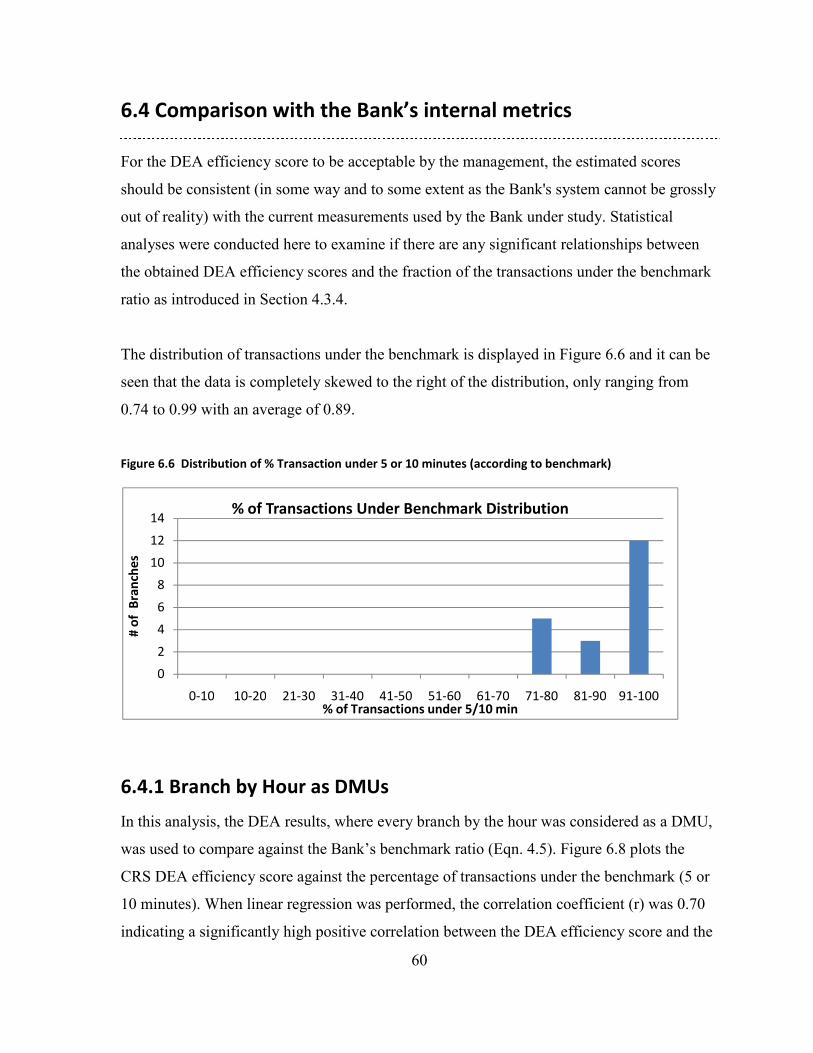
60
0
2
4
6
8
10
12
14
0-10 10-20 21-30 31-40 41-50 51-60 61-70 71-80 81-90 91-100
# of
Bra
nche
s
% of Transactions under 5/10 min
% of Transactions Under Benchmark Distribution
6.4 Comparison with the Bank’s internal metrics
For the DEA efficiency score to be acceptable by the management, the estimated scores
should be consistent (in some way and to some extent as the Bank's system cannot be grossly
out of reality) with the current measurements used by the Bank under study. Statistical
analyses were conducted here to examine if there are any significant relationships between
the obtained DEA efficiency scores and the fraction of the transactions under the benchmark
ratio as introduced in Section 4.3.4.
The distribution of transactions under the benchmark is displayed in Figure 6.6 and it can be
seen that the data is completely skewed to the right of the distribution, only ranging from
0.74 to 0.99 with an average of 0.89.
Figure 6.6 Distribution of % Transaction under 5 or 10 minutes (according to benchmark)
6.4.1 Branch by Hour as DMUs
In this analysis, the DEA results, where every branch by the hour was considered as a DMU,
was used to compare against the Bank’s benchmark ratio (Eqn. 4.5). Figure 6.8 plots the
CRS DEA efficiency score against the percentage of transactions under the benchmark (5 or
10 minutes). When linear regression was performed, the correlation coefficient (r) was 0.70
indicating a significantly high positive correlation between the DEA efficiency score and the
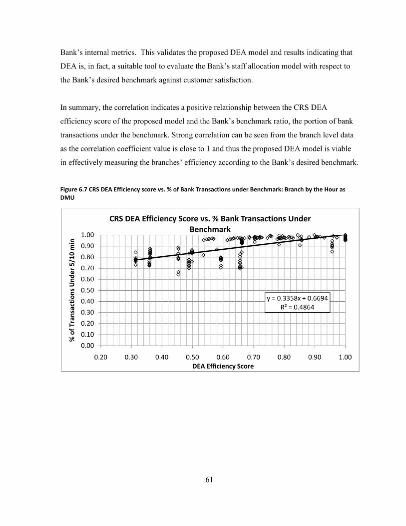
61
Bank’s internal metrics. This validates the proposed DEA model and results indicating that
DEA is, in fact, a suitable tool to evaluate the Bank’s staff allocation model with respect to
the Bank’s desired benchmark against customer satisfaction.
In summary, the correlation indicates a positive relationship between the CRS DEA
efficiency score of the proposed model and the Bank’s benchmark ratio, the portion of bank
transactions under the benchmark. Strong correlation can be seen from the branch level data
as the correlation coefficient value is close to 1 and thus the proposed DEA model is viable
in effectively measuring the branches’ efficiency according to the Bank’s desired benchmark.
Figure 6.7 CRS DEA Efficiency score vs. % of Bank Transactions under Benchmark: Branch by the Hour as DMU
y = 0.3358x + 0.6694R² = 0.4864
0.00
0.10
0.20
0.30
0.40
0.50
0.60
0.70
0.80
0.90
1.00
0.20 0.30 0.40 0.50 0.60 0.70 0.80 0.90 1.00
% o
f Tra
nsac
tion
s U
nder
5/1
0 m
in
DEA Efficiency Score
CRS DEA Efficiency Score vs. % Bank Transactions Under Benchmark
62
6.5 Chapter Summary
In this chapter, a DEA model was proposed to evaluate the efficiency of branch operations
meeting the desired service time benchmarks. Transaction by transaction data for a month
provided by the Bank was used to model a CRS non-controllable variable included DEA
model. After examining the distribution of average total transactions per day and distribution
of average total transactions per hour, it was found that the hourly transactional volume
indicated a significantly high variance that should be accounted for in the analysis. Thus, a
two part analysis was conducted using branch as a DMU and branch by hour (this is the
value when the transaction times are averaged on the hour) as a DMU.
CRS DEA model results revealed average efficiency scores of 78% and 65% for the DEA
model built upon branch as a DMU and branch by hour as a DMU, respectively. Average
efficiency scores were much higher when the branch was evaluated as a single DMU,
because of the small sample size and large percentage of efficient branches being self-
identifiers. One of the major shortcomings of DEA is its inability to evaluate small sample
size and when each hour was segregated to be accounted as a DMU, the result was much
more comprehensive with varying degree of efficiency scores across the distribution.
However, the lower average efficiency scores for hourly FTE data indicated that the BCM
still has improvement possibilities when allocating staff. Overall, the results support the
BCM’s effectiveness in meeting the desired service time benchmarks.
The CRS DEA model result were then compared to the Bank’s desired service time
benchmark ratio values (Section 4.3.4 – Equation 4.5) and showed a strong positive
correlation between the DEA efficiency scores and the Bank’s benchmark ratio scores. This
validates the proposed DEA model and results, and suggests that DEA is, in fact, a suitable
tool to evaluate the Bank’s staff allocation model’s efficacy with respect to the Bank’s
desired benchmarks.
63
CHAPTER 7:
CONCLUSIONS AND FINDINGS This chapter concludes the research presented in this thesis by summarizing the discovery
and contribution by this research for the Bank under study.
7.1 Key Analytic Contributions to the Bank’s Management
Process
This thesis provides a summary of DEA and its application to a major Canadian bank’s
branch network. It also compared DEA results to the Bank’s internal metrics to validate
DEA’s ability to evaluate its bank branches’ efficiencies. The DEA model results not only
evaluated the branch network efficiency but also identified areas for improvement and
suggested areas for further investigation for the Bank. This thesis provided the Bank a
practical methodology to evaluate their current model and can be used for future staff
allocation system’s considerations.
The DEA results provide the efficiency scores in the context of staffing only of each branch
in the Bank’s network. These scores captured how efficient or inefficient a branch is when
compared to other branches. The reference set and targets provided by DEA suggests to
management the type and amount of inputs and outputs changes are needed to improve each
branch’s performance.
Moreover, the factors affecting branch performance may be found by analyzing the
differences between efficient and inefficient branches. In-depth observations of the efficient
branches that appear frequently and significantly in peer groups for the inefficient branches
can provide insights into efficient operations can be conducted. In addition, other
environmental factors such as geographic regions, branch size and other model levers used in
64
BCM have shown indications to characteristic advantage between groups of branches, which
can be used to calibrate the staff allocation model to be a better fit.
The comparison of DEA and the Bank’s internal metrics provided an overview of DEA’s
ability to measure bank branch efficiencies. The most important contribution of this thesis is
the proposed model in evaluating the accuracy of the Bank’s staffing allocation model to
meet the desired customer satisfaction benchmark. Performance analysis is very important in
any industry as it can be seen from the amount of academic research dedicated to the field.
However, there are not many studies done from the perspective of customer satisfaction and
comparisons of DEA results to the Bank’s ratios and benchmarks for validity.
Overall, the DEA results and the analysis can be used to estimate the potential savings from
the improved performance. This research shows that the bank branches examined have a
potential for improvement and detailed analysis combined with field study could achieve
these improvements, hence accrue cost savings.
7.2 Findings Summary and Conclusions
This thesis developed DEA models in which the staffing allocation performance of the
Bank`s branch network under study was evaluated. Productivity and efficiency measurement
oriented DEA models were developed to evaluate the bank branch staffing allocation strategy
by using different types of DEA models including non-controllable - constant returns to scale
(CRS) and non-controllable - variable returns to scale (VRS). Two main DEA models were
developed, (1) to evaluate the overall efficiency of the BCM and the branch network from
strictly a staffing point of view and (2) to evaluate the accuracy of the BCM with respect to
the Bank’s benchmarks in achieving the desired customer satisfaction experience.
An overview of the Bank under study and the data were presented in detail in chapter 4. The
branches were classified into four major branch size groups: ‘small’, ‘medium-small’,
‘medium-large’ and ‘large’ branches, based on the number of FTEs, average weekly total
number of transactions and average weekly business transactions. The Bank’s performance
65
ratios and benchmark ratios were reviewed in detail to understand their effectiveness in
measuring their branches’ performance. The performance measuring ratios were found to be
not adequate for the purpose as both ratios showed a significantly high correlation to the
branch size, leading to a naturally lower efficiency score for smaller branches. Of course,
this is one of the serious problems with single ratios used in this context.
The DEA results included overall and individual branch efficiency scores, which were then
used to provide detailed managerial analysis. Overall, the comparison of CRS and VRS
results showed that the branches under study were operating at constant returns to scale.
Therefore, only the CRS results were used in chapter 6. In chapter 5, the DEA result showed
that 15% of the Bank’s branch network was efficient (efficiency = 1) and the average
efficiency score was 73%. This indicated BCM’s overall effectiveness in allocating CSR
staff across their national branch network however there is still significant potential for
improvement as DEA was able to identify well performing branches as well as inefficient
branches with efficiency scores ranging from 18% to the fully efficient, 100%. The DEA
results from chapter 5 were then compared against the Bank’s performance ratios. The
comparison showed insignificant correlation, supporting the weaknesses in traditional ratio
analyses for the use in measuring performance efficiency in the banking industry.
In chapter 6, the second DEA model proposed to evaluate the accuracy of the BCM’s
recommendation meeting the Bank’s desired service time benchmark, showed DEA result of
average efficiency score of 65% indicating BCM’s effectiveness yet much room for growth.
DEA results were then compared against the Bank’s customer satisfaction benchmarks and
this comparison indicated a strong correlation between the proposed DEA model and the
Bank’s benchmark ratio, validating the use of DEA for evaluating branch efficiency in
respect to the Bank’s desired customer satisfaction goals.
This thesis also provided a guideline for future performance analyses and a method for
comparisons to DEA, for other banks as well as other industries. Banks are highly regulated
in Canada and the large Canadian banks naturally adopt similar production technology and
66
operating methodology. Similar approaches could be taken by other banks in order to
evaluate their own staffing methodologies and discover areas for improvement.
In summary, DEA is a very useful analytical tool for management in all kinds of decision
making processes. In this study, DEA models were proposed to evaluate a major Canadian
bank’s staff allocating model from the context of meeting their desired customer satisfaction
benchmarks. Moreover, potential management use of DEA results were presented as each
branch efficiency score and target provides insights into improving branch performance.
Overall, this thesis provided valuable insights for management, regarding their current model
and in directing future operational improvements.
67
CHAPTER 8:
RECOMMENDATIONS AND FUTURE WORK This chapter provides recommendations for the Bank under study and possible areas of
future work.
8.1 Recommendations
The performance measurement ratios used by the Bank were found to be not adequate for the
purpose, as it has shown weakness in evaluating their branch network with its positive
correlation to the branch size. This study therefore recommends application of DEA in
efficiency measurement of the CSR allocation model, as DEA has widely been studied and
explored as a performance measurement tool in the banking industry and has showed
considerable success.
From the detailed analysis by branch size group and geographic region, DEA results
identified relatively inefficient branch groups such as ‘Medium-Small’ branches and in
region 3. These identified groups of branches should be further examined by the Bank to
reveal potential improvements in CSR staff allocation.
Overall, DEA efficiency scores revealed a high percentage of efficient branches and a high
average efficiency score of the national branch network supporting that the BCM is effective
in allocating CSR staff across the Bank’s branch network. Furthermore, DEA analysis done
on transaction-by-transaction data revealed a high efficiency average score in meeting the
Bank’s desired service time benchmark and once again, supporting BCM’s accuracy in
conforming to management’s desired inputs. However, DEA analysis done on hourly FTE
data revealed a lower average efficiency score indicating that the BCM has room to improve
in its guidance for branch operations to reach a maximum efficiency by hour.
68
As validated from this research, the proposed DEA model is recommended to be used by the
Bank’s management to identify efficient and inefficient branches in allocating CSR staff with
respect to meeting the Bank’s desired service time benchmark. This is a unique finding as not
many studies have taken the perspective of customer satisfaction and furthermore, validated
the proposed model’s viability against a bank’s actual desired benchmarks. With increasing
understanding of DEA and its effectiveness in efficiency analysis, there are more industry
friendly commercial software available for management’s use. The proposed DEA model can
be easily utilized by the Bank’s management by employing commercially available DEA
based software, to examine inputs and outputs changes needed to optimize each branch’s
operation.
8.2 Future Work
Further examination and statistical analysis of the DEA results provided in this research
could potentially reveal patterns for more effective branch operations such as the best staff
mix between part time and full time staff, best team mix (number of CSR teams) and much
more. Also, a limited sample size when evaluating the accuracy of BCM (Model #2) could
be eliminated by obtaining more branch breakdown data to produce results reflecting the
national branch network as well as hourly staff allocation efficiency. The proposed models
should be extended in the future not only to evaluate the high-level staff allocation model but
the branch manager level staff scheduling model to closely evaluate the branches’ efficiency
and identify more potential savings and improvement upon operations.
69
REFERENCES
[AIGN77] Aigner, D., Lovell, C.A. and Schmidt, P., “Formulation and estimation of stochastic frontier production function models”, Journal of Econometrics, vol. 6, pp. 21-37, 1977
[BANK84] Banker, R.D., Charnes, A., and Cooper, W.W., “Some Models for Estimating
Technical and Scale Inefficiencies in Data Envelopment Analysis”, Management Science, vol.30(9), pp.1078-1092, 1984.
[BANK86a] Banker, T.D., and Morey, R., “Efficiency Analysis for Exogenously Fixed Inputs and
Outputs”, Operations Research, vol.34 (4), pp. 513-521, 1986. [BANK86b] Banker, T.D., and Morey, R., “The Use of Categorical Variables in Data
Envelopment Analysis”, Management Science, vol.32 (12), pp. 1613-1627, 1986. [BAUE90] Bauer, P.W., “Recent developments in the econometric estimation of frontiers”,
Journal of Econometrics¸ vol. 46, pp. 39-56, 1990. [BAUE93] Bauer P.W. et al., “Efficiency and Productivity Growth in U.S. banking”, The
Measurement of Productive Efficiency: Techniques and Applications (H. O. Fried, C. A. K. Lovell, and S. S .Schmidt, eds.) New York: Oxford University Press, pp. 386-413, 1993.
[BAUE98] Bauer, P.W., Berger, A.N., Ferrier, G.D., and Humphrey, D.B., “Consistency
Conditions for Regulatory Analysis of Financial Institutions: A Comparison of Frontier Efficiency Methods”, Journal of Economics and Business, vol. 50, pp. 85-114, 1998
[BERG91] Berger, A.N., and Humphrey, D.B., “The Dominance of Inefficiencies over scale and
Product Mix Economies in Banking”, Journal of Monetary and Economics, vol.28 (1), pp. 117-148, 1991.
[BERG93] Berger, A.N., Hunter, W.C., and Timme, S.G., “The efficiency of financial
institutions: A review and preview of research past, present, and future”, Journal of Banking and Finance, vol. 17, pp. 221-249, 1993.
[BERG97] Berger, A.N., and Humphrey, D.B., “Efficiency of Financial Institutions:
International Survey and Directions for Future Research”, European Journal of Operational Research, vol. 98, pp. 175-212, 1997
70
[BERG98] Berger, A.N., and Hannan, T.H., “The Efficiency Cost of Market Power in the Banking Industry: A Test of the ‘Quiet Life’ and Related Hypotheses”, Review of Economics and Statistics, vol.80, pp.454-465, 1998
[CANA03] Canadian Bankers Association, [Online document], [Cited January 20, 2003],
Available http://www.cba.ca [CHAR78] Charnes, A., Coopers, W.W., and Rhodes, E., “Measuring the Efficiency of
Decision- Making Units”, European Journal of Operational Research, vol. 2(6), pp. 429-444, 1978.
[CHAR82] Charnes, A., Coopers, W.W., Seiford, L., and Stutz, J., “A Multiplicative Model for
Efficiency Analysis”, Socio – Economic Planning Sciences, vol. 16(5), pp. 223-224, 1982
[CHAR85] Charnes, A., Clark, C.T., Cooper, W.W., and Golany, B., “A Developmental Study
of Data Envelopment Analysis in Measuring the Efficiency of Maintenance Units in the US Air Forces”, Annals of Operations Research, vol. 2, pp. 95-112, 1985.
[CHAR89] Charnes, A., Coopers, W.W., Wei, Q.L., and Huang, Z.M., “Cone Ratio Data
Envelopment Analysis and Multi-Objective Programming”, International Journal of systems Science, vol. 20 (7), pp. 1099-1118, 1989.
[CHAR94] Charnes, A., Cooper, W.W., Lewin, A.Y., and Seiford, L.M., Eds, “Data
Envelopment Analysis: Theory, Methodology and Applications”, Kluwer Academic Publishers, 1994
[CHEN02] Chen, Y., and Ali, A.I., “Output-input ratio analysis and DEA frontier”, European
Journal of Operational Research, vol.142, pp. 476-479, 2002. [CLIN07] Clinebell, S.K., and Clinebell, J.M., “Differences between part-time and full-time
employees in the financial services industry”, Journal of Leadership & Organizational Studies, 2007
[COOK00] Cook, W.D., Hababou, M., and Tuenter, H.J., “Multicomponent efficiency measurement and shared inputs in data envelopment analysis: an application to sales and service performance in bank branches”, Journal of Productivity Analysis, vol. 14, pp. 209-224, 2000.
[COOP07] Cooper, W.W., Seiford, L.M., and Tone, K. (Eds.), “Data Envelopment Analysis: A
Comprehensive Text with Models, Applications, References and DEA-Solver Software”, Springer Science + Business Media, New York, Second Edition, 2007.
71
[DAS09] Das, A., Ray, S.C., and Nag, A., “Labor-use efficiency in Indian banking: A branch-level analysis”, Omega the International Journal of Management Science, vol. 37, pp. 411-425, 2009.
[DEBA06] Debasish, S.S., “Efficiency Performance in Indian Banking – Use of Data
Envelopment Analysis”, Global Business Review, 2006. [DEVI09] Deville, A., “Branch banking network assessment using DEA: A benchmarking
analysis – A note”, Management Accounting Research, vol. 20, pp. 252-261, 2009. [DYSO88] Dyson, R.G., and Thanassoulis, E., “Reducing Weight Flexibility in Data
Envelopment Analysis”, Journal of Operational Research Society, vol.39(6), pp. 563-576, 1988.
[EISE97] Eisenbeis, R.A., Ferrier, G.D., and Kwan, S. “The Informativeness of Linear
Programming and Econometric Efficiency Scores: An Analysis using U.S. banking data”, Working paper, Bureau of Business and Economic Research, University of Arkansas. 1997.
[EMRO08] Emrouznejad, A., Parker, B.R., and Tavares, G., “Evaluation of research in efficiency
and productivity: A survey and analysis of the first 30 years of scholarly literature in DEA”, Socio-Economic Planning Sciences, vol. 42, pp. 151-157, 2008
[FARR57] Farrell, M.J., "The measurement of productive efficiency". Journal of Royal Statistical
Society, Series A 120 (3), pp. 253-290, 1957. [FED03] A User’s Guide for the Bank Holding Company Performance Report, Board of
Governors of the Federal Reserve System Division of Banking Supervision and Regulation, Washington D.C., 2003.
[FERR90] Ferrier, G.D., and Lovell, C.A.K., “Measuring Cost Efficiency in Banking:
Econometric and Linear Programming Evidence”, Journal of Econometrics, vol.46 (1/2), pp.229-245, 1990.
[FETH10] Fethi, M.R., and Pasiouras, F., “Assessing bank efficiency and performance with
operational research and artificial intelligence techniques: A survey”, European Journal of Operational Research, vol. 204, pp. 189-198, 2010.
[GIOK08] Giokas, D.I., “Assessing the efficiency in operations of a large Greek bank branch
network adopting different economic behaviours”, Economic Modeling, vol. 25, pp.559-574, 2008.
72
[GREB99] Greboval, D., “Managing fishing Capacity: Selected Papers on Underlying concepts and Issues”, FAO Fisheries Technical Paper 386, Food and Agriculture Organization of the United Nations, Rome, Appendix XIV, 1999.
[HAAG95] Haag, S.E., and Jaska, P.V., “Interpreting Inefficiency Ratings: An Application of
Bank Branch Operating Efficiencies”, Managerial and Decision Economics, vol.16, pp.7-14, 1995.
[HASA96] Hasan, I., and Hunger W.C., “Efficiency of Japanese multinational banks in the U.S.”,
Research in Finance, vol.14 (A. H. Chen, ed.). Greenwich, CT: JAI Press, pp. 157-173, 1996.
[HO04] Ho, C., and Zhu, D., “Performance measurement of Taiwan’s commercial banks”,
International Journal of Productivity and Performance Management, vol.53, pp.425-434, 2004.
[HSIE10] Hsieh, L., and Lin, L., “A performance evaluation model for international tourist
hotels in Taiwan – An application of the relational network DEA”, International Journal of Hospitality Management, vol. 29, pp. 14-24, 2010
[KAO08] Kao, C. and Hwang, S.N., “Efficiency decomposition in two – stage data
envelopment analysis: an application to non-life insurance companies in Taiwan”, European Journal of Operational Research, vol. 185(1), pp. 418-429, 2008.
[LIU01] Liu, B., and Tripe, D., “New Zealand Bank Mergers and Efficiency Gains”, 14th
Annual Australian Finance and Banking Conference, Sydney, 2001 [LUO03] Luo, X., “Evaluating the profitability and marketability efficiency of large banks: An
application of data envelopment analysis”, Journal of Business Research, vol.56, pp.627-635, 2003.
[MEEU77] Meeusen, W., and Van Den Broeck, J., “Efficiency Estimation from Cobb-Douglas
Production Functions with Composed Error”, International Economic Review, vo. 18(2), pp. 435-444, 1977
[MOST09] Mostafa, M.M., “Modeling the efficiency of top Arab banks: A DEA – neural
network approach”, Expert Systems with Applications, vol. 36, pp. 309-320, 2009. [NFO03] NFO CFgroup Poll. “Tellers still popular, study finds”. The Globe and Mail; 2003,
January: B5 [ORAL90] Oral, M. and Yolalan, R., “An Empirical Study on Measuring Operating Efficiency
and Profitability of Bank Branches”, European Journal of Operational Research, 46, pp. 282-294, 1990.
73
[PARA04A] Paradi, J.C., Vela, S., and Yang, Z., “Assessing Bank and Bank Branch Performance
Modeling Considerations and Approaches”, International Series in Operations Research and Management Science, vol. 71, pp. 349-394, 2004.
[PARA04B] Paradi, C.J. and Schaffnit, C., “Commercial branch performance evaluation and
results communication in a Canadian bank – a DEA application”, European Journal of Operational Research, Vol. 156, pp. 719-35, 2004.
[PARA11] Paradi, J.C., Rouatt, S., and Zhu, H., “Two-stage evaluation of bank branch
efficiency using data envelopment analysis”, Omega, vol. 39, pp. 99-109, 2011. [PARK87] Parkan, C., “Measuring the efficiency of service operations: an application to bank
branches”, Engineering Costs and Production Economics, vol. 12, pp. 237-242, 1987.
[REST97] Resti, A., “Evaluating the cost-efficiency of the Italian banking system: What can be
learned from the joint application of parametric and nonparametric techniques?”, Journal of Banking and Finance, vol.20 (2), pp.221-250, 1997.
[ROUA03] Rouatt, S.J., “Two Stage Evaluation of Bank Branch Efficiency Using Data
Envelopment Analysis”, Masters Thesis, Centre for Management of Technology and Entrepreneurship (C.M.T.E.), University of Toronto, 2003.
[SCHA97] Schaffinit, C., Rosen, D., and Paradi, J.C., “Best practice analysis of bank branches:
an application of DEA in a Large Canadian Bank”, European Journal of Operational Research, vol. 98, pp. 269-289, 1997.
[SCHI90] Schinnar, A.P., et al., “Organizational determinants of efficiency and effectiveness in
mental health partial care programs”, Health Services Research, vol.25, pp. 387-420, 1990.
[SHER84] Sherman, H.D., “Improving the Productivity of Service Businesses”, Massachusetts
Institute of Technology, Sloan Management Review, pp. 11-23, 1984. [SHER85] Sherman, H.D., and Gold, F., “Bank Branch Operating Efficiency: Evaluation with
Data Envelopment Analysis”, Journal of Banking and Finance, vol. 9(2), pp. 297-316, 1985.
[SHER95] Sherman, H.D., and Ladino, G., “Managing Bank Productivity Using Data
Envelopment Analysis (DEA)”, Interfaces, vol. 25(2), pp. 60-73, 1995.
74
[SHIN90] Shinnar, A.P., Kamis-Gould, E., Delucia, N. and Rothbard, A.B., “Organizational determinants of efficiency and effectiveness in mental health partial care programs”, Health Services Research, vol. 25, pp. 387-420, 1990
[SOWL04] Sowlati, T. and Paradi, J.C., “Establishing the “practical frontier” in data
envelopment analysis”, International Journal of Management Science, vol. 32. Page 261-272. 2004
[THOM90] Thompson, R.G. et al., “The Role of Multiplier bounds in Efficiency Analysis
with Application to Kansas Farming”, Journal of Econometrics, vol.46, pp. 93-108, 1990.
[TOCH06] Tochaie, N.M., “Bank Branch Productivity Comparison – DEA Models with Bank
Methods”, Masters Thesis, Centre for Management of Technology and
Entrepreneurship (C.M.T.E.), University of Toronto, 2006.
[TULK93] Tulkens, H., “On FDH Efficiency Analysis: Some Methodological Issues and
Application to Retail Banking, Courts and Urban Transit”, Journal of Productivity
Analysis, vol.4 (1/2), pp. 183-210, 1993.
[VASS90] Vassiloglou, M., and Giokas, D., “A Study of the Relative Efficiency of Bank
Branches: An Application of Data Envelopment Analysis”, Journal of the
Operational Research Society, vol.41 (7), pp. 591-597, 1990.
[WANG97] Wang, C.H., Gopal, R.D. and Zionts, S., “Use of data envelopment analysis in
assessing information technology impact on firm performance”, Annals of Operations Research, vol. 73, pp. 191-123, 1997
[WU06] Wu, D., Yang, Z., and Liang, L., “Use DEA-neural network approach to evaluate
branch efficiency of a large Canadian bank”, Expert Systems with Applications, vol. 31, pp. 108-115, 2006.
75
GLOSSARY Allocative Efficiency Measure of the ability of a unit to use inputs in the most
optimal proportions given a set of prices.
Bank’s Current Staff A model that captures customer service staff allocation of a bank branch in terms of inputs needed for the branch to
allocation Model (BCM) operate and outputs produced from its operations. VRS or VRS Model DEA model which assumes a variable returns to scale
relationship between inputs and outputs.
BM Branch Manager
BCM See Bank`s Current staff allocating Model
Categorical Variable Variable that assumes a predefined set of discrete values.
CRS Model DEA model which assumes a constant returns to scale relationship
Correlation A measure of the strength of the relationship between two Coefficient variables. The value lies between +1 and -1.
CSR Customer Service Representative (Tellers)
CSR:Expert CSR Expert: Sub team of the CSR and is responsible for complex transactions such as foreign exchange
CT Central Teller: Sub team of the CSR and is responsible for business transactions
DEA Data Envelopment Analysis: Non-parametric, fractional linear programming approach, which calculates relative efficiencies of Decision - Making Units (DMUs) and requires no prior specification of the functional form of the frontier.
DFA Distribution Free Approach
DMU Decision Making Unit: A term used to describe a unit being analyzed in DEA
Econometric Approach A parametric approach for measuring efficiency, which requires a priori specification of the functional form.
EFA Econometric Frontier Approach.
76
Effectiveness The ability of an organization to achieve its pre-set goals and objectives. A measure of “Doing the right things”.
Efficiency The ability to attain the outputs with a minimum level of resources. A measure of doing things right.
Efficiency Gains Changes in efficiency from one point in time to another
Efficient Frontier Empirical frontier that represents “best performance” and consists of units in the data set, which is most efficient in transforming their inputs into outputs.
FDH Free Disposal Hull.
FTE Full-time-equivalent: Total number of full time positions required to complete the activities.
Input-Oriented Model A DEA model whose objective is to minimize inputs while keeping the outputs constant.
Intermediation Approach Approach in which a Financial Services Unit is viewed as a financial intermediary whose function is to invest deposits into profitable investments.
IO Input – Oriented Model
IRS Increasing Returns to Scale. A measure where a proportionate increase in inputs result in a more than proportionate increase in outputs.
MPSS Most productive scale size. The point on the efficient frontier at which maximum average productivity is achieved for a given input/output mix.
Non-Discretionary Variable/A variable over which the management does not have control Non-Controllable Variable and therefore, cannot alter its level of use or production Output-Oriented Model A DEA model where the objective is to maximize outputs
while keeping the inputs constant.
Overall Efficiency Efficiency measured as the product of technical and allocative efficiency.
Peer Group Set of efficient units to which the inefficient units are compared.
77
Production Approach Process in which inputs are transformed into outputs by a production unit.
Production Function Function in which outputs are defined as functions of inputs.
Productivity Defined as a ratio of outputs to inputs.
Relative Efficiency A measure of actual performance of a production unit relative to best-observed performance of other similar units.
Scale Efficiency Efficiency that indicates whether the unit is operating at its optimal size
SFA Stochastic Frontier Approach.
Slack Variable Represents the under-production of outputs or over-utilization of inputs in the DEA evaluation.
Target The value of the inputs and outputs, which would result in an inefficient unit becoming efficient.
Technical Efficiency Efficiency of the production process in converting inputs into outputs.
TFA Thick Frontier Approach.
Theoretical Frontier Frontier of best possible production.
VRS Variable returns-to-scale. A measure where a proportionate increase in inputs could result in a proportionate increase or decrease in outputs.
Weights/Multipliers Coefficients applied to inputs and outputs.