Mon. Not. R. Astron. Soc. 000, 000–000 (0000) Printed 10 September 2015 (MN LATEX style file v2.2)

European Pulsar Timing Array Limits On An Isotropic StochasticGravitational-Wave Background

L. Lentati1?, S. R. Taylor2,3, C. M. F. Mingarelli4,5,6, A. Sesana6,7, S. A. Sanidas8,9,A. Vecchio6, R. N. Caballero5, K. J. Lee10,5, R. van Haasteren3, S. Babak7, C. G.Bassa11,9, P. Brem7, M. Burgay12, D. J. Champion5, I. Cognard13,14, G. Desvignes5, J.R. Gair2, L. Guillemot13,14, J. W. T. Hessels11,8, G. H. Janssen11,9, R. Karuppusamy5,M. Kramer5,9, A. Lassus5,15, P. Lazarus5, K. Liu5, S. Osłowski17,5, D. Perrodin12, A.Petiteau15, A. Possenti12, M. B. Purver9, P. A. Rosado18,19, R. Smits11, B. Stappers9, G.Theureau13,14,16, C. Tiburzi20,12, J. P. W. Verbiest17,5

1 Astrophysics Group, Cavendish Laboratory, JJ Thomson Avenue, Cambridge, CB3 0HE, UK2 Institute of Astronomy, University of Cambridge, Madingley Road, Cambridge CB3 0HA3 Jet Propulsion Laboratory, California Institute of Technology, Pasadena, California 91109, USA4 TAPIR (Theoretical Astrophysics), California Institute of Technology, Pasadena, California 91125, USA5 Max-Planck-Institut fur Radioastronomie, Auf dem Hugel 69, D-53121 Bonn, Germany6 School of Physics and Astronomy, University of Birmingham, Edgbaston, Birmingham B15 2TT, United Kingdom7 Max-Planck-Institut fur Gravitationsphysik, Albert Einstein Institut, Am Muhlenberg 1, 14476 Golm, Germany8 Anton Pannekoek Institute for Astronomy, University of Amsterdam, Science Park 904, 1098 XH Amsterdam, The Netherlands9 Jodrell Bank Centre for Astrophysics, University of Manchester, Manchester, M13 9PL, United Kingdom10 Kavli institute for astronomy and astrophysics,Peking University, Beijing 100871,P.R.China11 ASTRON, the Netherlands Institute for Radio Astronomy, Postbus 2, 7990 AA, Dwingeloo, The Netherlands12 INAF - Osservatorio Astronomico di Cagliari, via della Scienza 5, I-09047 Selargius (CA), Italy13 Laboratoire de Physique et Chimie de l’Environnement et de l’Espace LPC2E CNRS-Universite d’Orleans, F-45071 Orleans, France14 Station de radioastronomie de Nancay, Observatoire de Paris, CNRS/INSU F-18330 Nancay, France15 Universite Paris-Diderot-Paris7 APC - UFR de Physique, Batiment Condorcet ,10 rue Alice Domont et Leonie Duquet 75205 PARIS CEDEX 13, France16 Laboratoire Univers et Theories LUTh, Observatoire de Paris, CNRS/INSU, Universit Paris Diderot, 5 place Jules Janssen, 92190 Meudon, France17 Fakultat fur Physik, Universitat Bielefeld, Postfach 100131, 33501 Bielefeld, Germany18 Centre for Astrophysics & Supercomputing, Swinburne University of Technology, PO Box 218, Hawthorn VIC 3122, Australia19 Max Planck Institute for Gravitational Physics, Albert Einstein Institute, Callinstraße 38, 30167, Hanover, Germany20 Dipartimento di Fisica - Universita di Cagliari, Cittadella Universitaria, I-09042 Monserrato (CA), Italy

10 September 2015

ABSTRACTWe present new limits on an isotropic stochastic gravitational-wave background (GWB) usinga six pulsar dataset spanning 18 yr of observations from the 2015 European Pulsar TimingArray data release. Performing a Bayesian analysis, we fit simultaneously for the intrinsicnoise parameters for each pulsar, along with common correlated signals including clock, andSolar System ephemeris errors, obtaining a robust 95% upper limit on the dimensionless strainamplitude A of the background of A < 3.0 × 10−15 at a reference frequency of 1yr−1 and aspectral index of 13/3, corresponding to a background from inspiralling super-massive blackhole binaries, constraining the GW energy density to Ωgw( f )h2 < 1.1 × 10−9 at 2.8 nHz. Wealso present limits on the correlated power spectrum at a series of discrete frequencies, andshow that our sensitivity to a fiducial isotropic GWB is highest at a frequency of ∼ 5×10−9 Hz.Finally we discuss the implications of our analysis for the astrophysics of supermassive blackhole binaries, and present 95% upper limits on the string tension, Gµ/c2, characterising abackground produced by a cosmic string network for a set of possible scenarios, and for astochastic relic GWB. For a Nambu-Goto field theory cosmic string network, we set a limitGµ/c2 < 1.3×10−7, identical to that set by the Planck Collaboration, when combining Planckand high-` Cosmic Microwave Background data from other experiments. For a stochastic relicbackground we set a limit of Ωrelic

gw ( f )h2 < 1.2×10−9, a factor of 9 improvement over the moststringent limits previously set by a pulsar timing array.

c© 0000 RAS

arX

iv:1

504.

0369

2v3

[as

tro-

ph.C

O]

9 S

ep 2

015

2 L. Lentati et al.

1 INTRODUCTION

The first evidence for gravitational-waves (GWs) was originally ob-tained through the timing of the binary pulsar B1913+16. The ob-served decrease in the orbital period of this system was found tobe completely consistent with that predicted by general relativity,if the energy loss was due solely to the emission of gravitationalradiation (Taylor & Weisberg 1989). Despite a decrease of only2.3ms over the course of 30 yr, by exploiting the high precisionwith which the time of arrival (TOA) of electromagnetic radiationfrom pulsars can be measured, deviations from general relativityhave been constrained by this system to be less than 0.3% (Weis-berg, Nice & Taylor 2010).

Since then, observations of the double-pulsar, PSRJ0737−3039, have provided even greater constraints, placinglimits on deviations from general relativity of less than 0.05%(Kramer et al. (2006), Kramer et al. in prep.). It is this extraor-dinary precision that also makes pulsar timing one possible routetowards the direct detection of GWs, which remains a key goal inexperimental astrophysics.

For a detailed review of pulsar timing we refer to Lorimer &Kramer (2005). In general, one computes the difference betweenthe expected arrival time of a pulse, given by a pulsar’s timingmodel which characterises the properties of the pulsar’s orbital mo-tion, as well as its timing properties such as its spin frequency, andthe actual arrival time. The residuals from this fit then carry phys-ical information about the unmodelled effects in the pulse propa-gation, including those due to GWs (e.g. Sazhin 1978; Detweiler1979).

Individual pulsars have, for several decades, been used to setlimits on the amplitude of gravitational radiation from a range ofsources (e.g. Kaspi, Taylor & Ryba 1994). However, by using acollection of millisecond pulsars, known as a pulsar timing array(PTA, Foster & Backer 1990), one can both increase the signal-to-noise ratio of the effect of gravitational radiation in the timingresiduals, and use the expected form for the cross correlation of thesignal between pulsars in the array to discriminate between the GWsignal of interest, and other sources of noise in the data, such as theintrinsic spin-noise due to rotational irregularities (e.g. Shannon &Cordes 2010), or delays in the pulse arrival time due to propagationthrough the interstellar medium (e.g. Keith et al. 2013). In the spe-cific case of an isotropic stochastic gravitational-wave background(GWB), which is the focus of this paper, this correlation is knownas the ‘Hellings-Downs’ curve (Hellings & Downs 1983), and isonly a function of the angular separation of pairs of pulsars in thearray.

The lowest frequency to which a particular pulsar timingdataset will be sensitive is set by the total observing span for thatdataset. Sensitivity to frequencies lower than this is significantlydecreased due to the necessity of fitting a quadratic function in thepulsar timing model describing its spin down. PTA datasets are nowentering the regime where observations span decades, and as suchare most sensitive to GWs in the range 10−9−10−8 Hz. The primaryGW sources in this band are thought to be supermassive black holebinaries (SMBHBs) (Rajagopal & Romani 1995; Jaffe & Backer2003; Wyithe & Loeb 2003; Sesana et al. 2004; Sesana, Vecchio& Colacino 2008), however other sources such as cosmic strings(see, e.g. Vilenkin 1981; Vilenkin & Shellard 1994) or relics frominflation (see, e.g. Grishchuk 2005) have also been suggested.

The formation of SMBHBs is a direct consequence of the hi-erarchical structure formation paradigm. There is strong evidencethat SMBHs are common in the nuclei of nearby galaxies (see Kor-

mendy & Ho 2013, and references therein). The fact that many dis-tant galaxies harbour active nuclei for a short period of their life im-plies that they were also common in the past. In Λ-Cold Dark Mat-ter (Λ-CDM) cosmology models galaxies merge frequently (Lacey& Cole 1993). During a galaxy merger the SMBHs harboured in thegalactic nuclei will sink to the center of the merger remnant, even-tually forming a SMBHB (Begelman, Blandford & Rees 1980). Asa consequence the Universe should contain a potentially large num-ber of gradually in-spiralling SMBHBs. The incoherent superposi-tion of GWs from these binaries is expected to form an isotropicstochastic GWB. Deviations from isotropy, however, such as froma small number of bright nearby sources, could result in individ-ually resolvable systems (Lee et al. 2011), and an anisotropic dis-tribution of power across the sky (Mingarelli et al. 2013; Taylor &Gair 2013; Gair et al. 2014). These latter situations are the subjectof two companion papers (Taylor et al. 2015; Babak et al. 2015)here we focus on the possibility of detecting a stochastic isotropicGWB, and we will discuss the implications of our findings for theastrophysics of SMBHBs, cosmic strings, and relics from inflation.

An isotropic, stochastic GWB of cosmological or astrophysi-cal origin can be described in terms of its GW energy density con-tent ρgw per unit logarithmic frequency, divided by the critical en-ergy density, ρc, to close the Universe:

Ωgw( f ) =1ρc

dρgw

d ln f=

2π2

3H20

f 2h2c( f ). (1)

Here, f is the GW frequency, ρc = 3H20/8π is the critical energy

density required to close the Universe, H0 = 100 h km s−1 Mpc−1 isthe Hubble expansion rate, with h the dimensionless Hubble param-eter, and ρgw is the total energy density in GWs (Allen & Romano1999; Maggiore 2000).

Typically the ‘characteristic strain’, hc( f ), associated with aGWB energy density Ωgw( f ) is parametrised as a single power-lawfor several backgrounds of interest:

hc = A(

fyr−1

)α, (2)

where A is the strain amplitude at a characteristic frequency of1yr−1, and α describes the slope of the spectrum. Finally, hc is di-rectly related to the observable quantity induced by a GWB in ourtiming residuals, the one-sided power spectral density, S ( f ), givenby:

S ( f ) =1

12π2

1f 3 hc( f )2 =

A2

12π2

(f

yr−1

)−γyr3, (3)

where γ ≡ 3 − 2α. Note that unless explicitly stated otherwise,henceforth when referring to spectral indices we will be referringto the quantity γ.

The expected spectral index varies depending on the source ofthe stochastic background. For a GWB resulting from inspiralingSMBHBs the characteristic strain is approximately hc( f ) ∝ f −2/3

(Rajagopal & Romani 1995; Jaffe & Backer 2003; Wyithe & Loeb2003; Sesana et al. 2004), or equivalently, γ = 13/3, whereas pri-mordial background contributions or cosmic strings are expected tohave power-law indices of γ = 5 (Grishchuk 2005), and γ = 16/3(Olmez, Mandic & Siemens 2010; Damour & Vilenkin 2005) re-spectively. However, for cosmic strings in particular, a single spec-tral index is not expected to accurately describe the spectrum in thePTA frequency band (Sanidas, Battye & Stappers 2012).

A multitude of experiments have set limits on the amplitudeof the stochastic GWB, either at a reference frequency as is donefor PTAs (Shannon et al. 2013) and ground-based interferome-

c© 0000 RAS, MNRAS 000, 000–000

EPTA Limits 3

10−9 10−8 10−7

Observed GW frequency [Hz]

10−12

10−11

10−10

10−9

10−8

10−7

10−6

10−5

10−4

10−3

Ωgw

(f)

BBN + CMB

Spectral estimation

SMBH binary limit

Relic limit

Cosmic string limit

f = 1yr−1

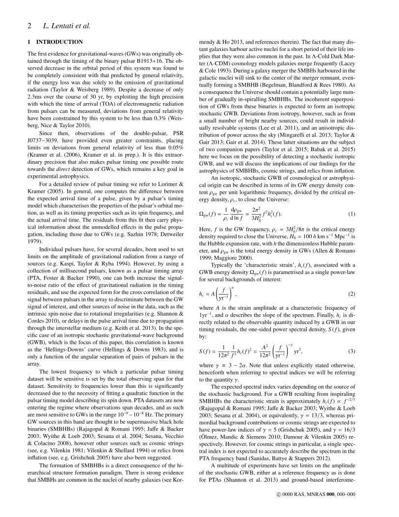
Figure 1. Summary of key results from the analysis of a 6 pulsar dataset from the 2015 EPTA data release (D15). Results are presented in terms of Ωgw( f ) as afunction of GW frequency, with H0 = 70km s−1 Mpc−1. We indicate the 95% upper limits on the amplitude of a correlated GWB assuming a power law modelwith a spectral index of γ = 13/3 (solid black line; Section 5) and for a more general analysis where the power is determined simultaneously at a set of discretefrequencies (dashed line) as discussed in Section 5.1.1. The red shaded areas represent the central 68%, 95%, and 99.7% confidence interval of the predictedGWB amplitude according to Sesana (2013b) under the assumptions that a SMBHB evolves purely due to gravitational radiation reaction and binaries arecircular (See Section 6.1 for more details). Only about 5% of the distribution is excluded, meaning that our limit does not place significant restrictions on thecosmic SMBHB population. We also indicate 95% upper limits obtained for a stochastic relic background (green dash-dotted line; Section 6.3), and for cosmicstring network backgrounds (blue triple-dashed line; Section 6.2). The cosmic string limit plotted corresponds to a fiducial model for a population of cosmicstrings, with the following parameters: string tension Gµ/c2 = 10−7, the birth-scale of loops relative to the horizon αcs = 1.6 × 10−6, spectral index q = 4/3,cut-off on the number of emission harmonics n∗ = 1 and intercommutation probability p = 1. Finally we indicate recent constraints placed by CMB (Sendra& Smith 2012), and BBN (Allen 1997; Maggiore 2000; Planck Collaboration et al. 2015) observations.

ters (Aasi et al. 2014), or by reporting a value for GW energy den-sity integrated over all frequencies as is done by Big Bang Nu-cleosynthesis measurements, e.g. (Cyburt et al. 2005) and CosmicMicrowave Background (CMB) measurements (Smith, Pierpaoli &Kamionkowski 2006; Sendra & Smith 2012). As such, an upperlimit on the stochastic GWB reported in terms of either Ωgw( f )h2,or Ωgw( f ) for a specified value of h provides a clear way to reportour limits.

In the last few years the European PTA (EPTA), Parkes PTA(PPTA), and the North American NanoHertz Observatory for Grav-itational waves (NANOGrav) have placed 95% upper limits onthe amplitude of a stochastic GWB at a reference frequency of1yr−1 of 6×10−15 (van Haasteren et al. 2011), 2.4×10−15 (Shan-non et al. 2013), and 7×10−15 (Demorest et al. 2013) respectively.While many of the same pulsars are used by all the PTAs, andboth the EPTA and PPTA have similar total observing spans, allof these limits have been placed using different datasets, and dif-ferent methodologies. As such, these similarly constraining limitsshould not be seen as redundant, but rather as complementary. Forexample, the first EPTA limit used Bayesian analysis methods, pro-ducing an upper limit while simultaneously fitting for the intrinsictiming noise of the pulsars. Subsequent limits have used simula-tions to obtain conservative upper bounds consistent with the data,

or made use of frequentist methods, fixing the noise at values de-rived from analysis of the individual pulsars. Naturally a simultane-ous analysis of the intrinsic properties of the pulsars with the GWBis the preferred method, and we will show explicitly in Section 5that fixing the noise properties of the individual pulsars can lead toan erroneously stringent limit on the amplitude of a GWB in thepulsar timing data. The three PTA projects also work together asthe International PTA (IPTA; Hobbs et al. 2010), where all threedatasets are combined in order to produce ever more robust andconstraining limits on the GWB, with the eventual goal of makinga first detection.

In this work we make use of the Bayesian methods presentedin Lentati et al. (2013) (henceforth L13), which allows us to greatlyextend what is computationally feasible for a Bayesian analysis ofpulsar timing data. In particular, while we obtain upper limits onthe amplitude of a GWB using a simple, two parameter power lawas in van Haasteren et al. (2011), we can also make use of a muchmore general model, enabling us to place robust limits on the corre-lated power spectrum at discrete frequencies. We can also includeadditional sources of common noise in our analysis simultaneouslywith the GWB, such as those that could be expected from errorsin the Solar System ephemeris, or in the reference time standardused to measure the TOAs of the pulses. Finally we also take two

c© 0000 RAS, MNRAS 000, 000–000

4 L. Lentati et al.

approaches to parameterising the spatial correlations between pul-sars, without having to assume anything about the form it mighttake. This spatial correlation is the ‘smoking gun’ of a signal froma GWB, and so the ability to extract it directly from the data is cru-cial for the credibility of any future detections from pulsar timingdata.

The key results of our analysis, compared to current theoreti-cal predictions for a range of models of stochastic background andindirect limits in the PTA range are summarised in Fig. 1. In Sec-tion 2 we describe the deterministic and stochastic models that weincluded in this analysis. In Section 3 we discuss the implementa-tion of these methods in our Bayesian and frequentist frameworks.In Section 4 we introduce the EPTA dataset adopted for the analysis(Desvignes et al. in prep.), and in Section 5 we present the resultsobtained from our analysis. The implications of our findings forSMBHB astrophysics, cosmic strings, and relics from inflation arediscussed in Section 6, and finally, in Section 7 we summarise anddiscuss future prospects.

This research is the result of the common effort to directlydetect gravitational-waves using pulsar timing, known as the EPTA(EPTA; Kramer & Champion 2013) 1.

2 SIGNAL AND NOISE MODELS

The search for a stochastic GWB in pulsar timing data requiresthe estimation of a correlated signal of common origin in the pulseTOAs recorded for the different pulsars in the array. The difficultylies in the intrinsic weakness of the signal and the presence of arange of effects – both deterministic and stochastic – that conspireto mask the signal of interest. At the heart of our analysis methodsis the variance-covariance matrix

ΨIJ[i, j] = 〈dI[i]dJ[ j]〉 , (4)

that describes the expectation value of the correlation between TOAi from pulsar I, with a TOA j from pulsar J. In the followingdescription upper-case latin indices I, J, . . . identify pulsars, andlower case latin indices i, j, . . . are short hand notation for the TOAsti, t j, . . .. Eq. (4) depends on the unknown parameters that describethe model adopted to describe the data and enter the likelihoodfunction in the Bayesian analysis, and the optimal statistic in thefrequentist approach.

For any pulsar we adopt a model for the observed pulse TOAs,which we denote d, that results from a number of contributions andphysical effects according to:

d = τTM + τWN + τSN + τDM + τCN + τGW . (5)

In Eq. (5) we have:

• τTM, the deterministic model that characterises the pulsar’s as-trometric properties, such as position and proper motion, as well asits timing properties, such as spin period, and additional orbital pa-rameters if the pulsar is in a binary.• τWN, the stochastic contribution due to the combination of in-

strumental thermal noise, and intrinsic pulsar white noise.• τSN, the stochastic contribution due to red spin-noise.• τDM, the stochastic contribution due to changes in the disper-

sion of radio pulses traveling through the interstellar medium.

1 www.epta.eu.org/

• τCN, the stochastic contribution due to ‘common noise’,present across all pulsars in the timing array (described in Sec. 2.6),as could be expected from errors in the Solar System ephemeris, orin the reference time standard used to measure the TOAs of thepulses.• τGW, the stochastic contribution due to a GWB.

Our model assumes that all stochastic contributions are zeromean random Gaussian processes. Each of the contributions justdescribed depends on a number of unknown parameters that needto be simultaneously estimated in the analysis. While all these el-ements, which we set out in detail below, will be present in theBayesian analysis described in Section 3.1, we do not incorporatethe common pulsar noise terms in the frequentist optimal-statisticanalysis described in Section 3.2 as this approach by design in-terprets all cross-correlated power as originating from a stochasticGWB.

2.1 The timing model

The first contribution to the total signal model that we must con-sider is the deterministic effect due to the intrinsic evolution ofthe ‘pulsar clock’, encapsulated by the pulsar’s timing ephemeris.We identify with εI the m-dimensional parameter vector for pul-sar I that describes the relevant set of timing model parame-ters, and denote as τ(ε) the set of arrival times determined bythe adopted model and specific value of the parameters. We useTempo2 (Hobbs, Edwards & Manchester 2006; Edwards, Hobbs& Manchester 2006) to construct a weighted least-squares fit, inwhich the stochastic contributions have been determined from aBayesian analysis of the individual pulsars using the TempoNestplugin (Lentati et al. 2014). We can define the set of ‘post-fit’ resid-uals that results from subtracting the predicted TOA for each pulseat the Solar System Barycenter from our observed TOAs as:

dpost = d − τ(ε). (6)

In everything that follows, rather than use the full non-linear tim-ing model we consider an initial estimate of the m timing modelparameters ε0, and construct a linear approximation to that modelsuch that any deviations from those initial estimates are encapsu-lated using the m parameters δε such that:

δεi = εi − ε0i. (7)

Therefore, we can express the change in the post-fit residuals thatresults from the deviation in the timing model parameters δε as:

δt = dpost −Mδε, (8)

where M is the Nd × m ‘design matrix’ which describes the depen-dence of the timing residuals on the model parameters.

When we perform our Bayesian GWB analysis, we willmarginalise analytically over the linear timing model, as describedin Section 3.1. When performing this marginalisation the matrix Mis numerically unstable. To remedy this issue we follow the sameprocess as in van Haasteren & Vallisneri (2014) and take the SVDof M, to form the set of matrices USVT . Here U is an Nd×Nd matrix,which we can divide into two components:

U =(GC,G

), (9)

where G is a Nd × (Nd − m) matrix, which can be thought of as aprojection matrix (van Haasteren & Levin 2013), and GC is the Nd×

m complement. GC represents a set of orthonormal basis vectorsthat contain the same information as M but is stable numerically.We therefore replace M with GC in the subsequent analysis.

c© 0000 RAS, MNRAS 000, 000–000

EPTA Limits 5

2.2 White noise

We next consider the contribution to the total signal model thatresults from a stochastic white noise component, τWN. This noisecomponent is usually divided into two components, and this is themodel that we adopt in our analysis:

• For a given pulsar I, each TOA has an associated error bar,σ(I,i), the size of which will vary across a set of observations. Wecan introduce an extra free parameter, referred to as EFAC, toaccount for possible mis-calibration of this radiometer noise. TheEFAC parameter therefore acts as a multiplier for all the TOA errorbars for a given pulsar, observed with a particular ‘system’ (i.e. aunique combination of telescope, recording system and receiver).

• A second white noise component is also used to representsome additional source of time independent noise, which we callEQUAD, and adds in quadrature to the TOA error bar. In princi-ple this parameter represents something physical about the pulsar,for example, contributions from the high frequency tail of the pul-sar’s red spin-noise power spectrum, or jitter noise that results fromthe time averaging of a finite number of single pulses to form eachTOA (see e.g. Cordes & Downs 1985; Liu et al. 2011; Shannonet al. 2014). While this term should be independent of the observingsystem used to generate a given TOA, differences in the integrationtimes between TOAs for different observing epochs can muddy thisphysical interpretation.

We can therefore modify the uncertainty σ(I,i), defining σ(I,i) suchthat the statistical description is:

〈τWNI [i]τWN

J [ j]〉 = δIJδi jσ2(I,i) (10)

where

σ2(I,i) = (α(I,i)σ(I,i))2 + β2

(I,i) (11)

where α and β represent the EFAC and EQUAD parameters appliedto TOA i for pulsar I respectively. In Section 4 we list the numberof different observing systems per pulsar used in the analysis pre-sented in this paper.

2.3 Spin-noise

Individual pulsars are known to sometimes suffer from ‘spin-noise’,which is observed in the pulsar’s residuals as a red noise process.This is a particularly important noise source, as most models fora stochastic GWB predict that this too will induce a red spectrumsignal in the timing residuals. The spin-noise component is specificto each individual pulsar, and is uncorrelated between pulsars in thetiming array. The statistical properties of the spin-noise signal aretherefore given by:

〈τSNI [i]τSN

J [ j]〉 = δIJCSN(I,i, j), (12)

where the matrix element CSN(I,i, j) denotes the covariance in the spin-

noise signal between residuals i, j for pulsar I. In order to constructthe matrix CSN, we will use the time-frequency method describedin L13, which we will summarise below.

We begin by writing the spin-noise component of the stochas-tic signal as

τSN = FSNaSN (13)

where the matrix FSN denotes the Fourier transform such that forsignal frequency ν and time t we will have both:

FSN(ν, t) = sin (2πνt) , (14)

and an equivalent cosine term, and aSN are the set of free parametersthat describe the amplitude of the sine and cosine components ateach frequency.

We include in our model the set of frequencies with valuesn/T , where T the longest period to be included in the model andthe number of frequencies to be sampled is nSN. In our analysispresented in Section 4 we take T to be ∼ 18 yr, which is the to-tal observing span across all the pulsars in our dataset, and wetake nSN = 50 such that we include in our model periods up to∼ 130 days which is sufficient to describe the stochastic signalspresent in the data (Caballero et al. in prep.). For typical PTA dataLee et al. (2012) and van Haasteren & Levin (2013) showed thattaking T to be the longest time baseline in the dataset is sufficientto accurately describe the expected long-term variations present inthe data, as the quadratic term present in the timing model signifi-cantly diminishes our sensitivities to periods longer than this in thedata.

The covariance matrix of the spin-noise coefficients aSN be-tween pulsars I, J at model frequencies i, j, which we denote ΨSN

(I,J)will be diagonal, with components:

ΨSN(I,J,i, j) =

⟨aSN

(I,i)aSN(J, j)

⟩= ϕSN

I,i δi jδIJ , (15)

where the set of coefficients ϕSNI represent the theoretical power

spectrum of the spin-noise signal present in pulsar I. In our analysisof the dataset presented in Section 4 we assume that this intrinsicspin-noise can be well described by a 2-parameter power law modelin frequency, given by:

ϕSN(ν, ASN, γSN) =A2

SN

12π2

(1

1yr

)−3ν−γSN

T, (16)

with ASN and γSN the amplitude and spectral index of the powerlaw.

We note that as discussed in L13, whilst Eq. (15) states thatthe spin-noise model components are orthogonal to one another,this does not mean that we assume they are orthogonal in the timedomain where they are sampled, and it can be shown that this non-orthogonality is accounted for within the likelihood (van Haasteren& Vallisneri 2015). The covariance matrix CSN

I for the red noisesignal present in the data alone can then be written:

CSNI = N−1

I − N−1I FSN

I

[(FSN

I )T N−1I FSN

I + (ΨSN)−1]−1

(FSNI )T N−1

I , (17)

with NI the diagonal matrix containing the TOA uncertainties, suchthat N(I,i, j) = σ2

(I,i)δi j.

2.4 Dispersion measure variations

The plasma located in the interstellar medium (ISM) can result indelays in the propagation of the pulse signal between the pulsar andthe observatory. Variations in the column-density of this plasmaalong the line of sight to the pulsar can appear as a red noise signalin the timing residuals.

Unlike other red noise signals however, the severity of the ob-served dispersion measure (DM) variations is dependent upon theobserving frequency, and as such we can use this additional infor-mation to isolate the component of the red noise that results fromthis effect.

In particular, the group delay tg(νo) at an observed frequencyνo is given by the relation:

tg(νo) = DM/(Kν2o) (18)

c© 0000 RAS, MNRAS 000, 000–000

6 L. Lentati et al.

where the dispersion constant K is defined to be:

K ≡ 2.41 × 10−16 Hz−2 cm−3 pc s−1 (19)

and the DM is defined as the integral of the electron density ne fromthe Earth to the pulsar:

DM =

∫ L

0nedl . (20)

While many different approaches to performing DM correc-tion exist (e.g. Lee et al. (2014); Keith et al. (2013)), in our analysiswe use the methods described in L13. DM corrections can then beincluded in the analysis as an additional set of stochastic parametersin a similar manner to the intrinsic spin-noise. Further details onthe DM variations present in the EPTA dataset, including compar-isons between different models, will be presented in a seperate pa-per (Janssen et al. in prep.). In our analysis, as for the spin-noise, weassume a 2-parameter power law model, with an equivalent form toEq. (16), however we omit the factor 12π2 for the DM variations.

We first define a vector D of length Nd for a given pulsar as:

Di = 1/(Kν2(o,i)) (21)

for observation i with observing frequency ν(o,i).We then make a change to Eq. (14) such that our DM Fourier

modes are described by:

FDM(ν, ti) = sin (2πνti) Di (22)

and an equivalent cosine term, where the set of frequencies to beincluded is defined in the same way as for the red spin-noise, suchthat we choose the number of frequencies, nDM, to also be 50. Un-like when modelling the red spin-noise, where the quadratic termsin the timing model that accounts for pulsar spin-down acts as aproxy to the low frequency (ν < 1/T ) fluctuations in our data, weare still sensitive to the low frequency power in the DM signal. Assuch these terms must be accounted for either by explicitly includ-ing these low frequencies in the model, or by including a quadraticterm in DM to act as a proxy, defined as:

QDM(ti) = q0tiDi + q1t2i Di (23)

with q0,1 free parameters to be fit for, and ti the barycentric arrivaltime for TOA i. This can be achieved most simply by adding thetiming model parameters DM1 and DM2 into the pulsar timingmodel, which are equivalent to q0 and q1 in Eq. (23), and this is theapproach we take in our analysis here.

As for the spin-noise component we can then write down thetime domain signal for our DM variations as:

τDM = FDMaDM, (24)

with aDM the set of free parameters that describe the amplitude ofthe sine and cosine components at each frequency.

The covariance matrix of the coefficients aDM between pulsarsI, J at model frequencies i, j, which we denote ΨDM

(I,J) is then equiv-alent to the spin-noise matrix in Eq. (15), and we can similarilyconstruct the covariance matrix for the signal, τDM, as in Eq. (17).

2.5 Combining model terms

In order to simplify notation from this point forwards, for eachpulsar I we combine the matrices GC

I , FSNI and FDM

I into a single,Nd,I × (mI +2nSN +2nDM) matrix, where Nd,I is the number of TOAsin pulsar I, mI is the number of timing model parameters, and thefactor 2 in front of both nSN and nDM accounts for the sine and

cosine terms included for each model frequency. We denote thiscombined matrix TI , such that:

TI =(GC

I ,FSNI ,FDM

I

), (25)

and similarily we append the vectors δε,I , aSN, I , and aDM, I to formthe single vector bI . In this way we can write our complete signalmodel for a single pulsar I as:

τI = TIbI. (26)

We can then construct the block diagonal matrix T such thateach block is given by the matrix TI for each pulsar I, and finallyappend the set of vectors bI for all pulsars to form the completevector of signal coefficients b. In this way the concatenated signalmodel as described thus far for all pulsars, which we denote hereas τ, can be written simply:

τ = Tb. (27)

2.6 Common noise

In Tiburzi (2015 PhD Thesis) and Tiburzi et al. (2015, in prep.) itwas shown that additional sources of noise which are common toall pulsars in the PTA can be highly correlated with the quadrupolesignature of a stochastic GWB. If these sources of noise are presentin our dataset, we will become less sensitive to a GWB if we do notinclude them in our model. Therefore, in order to ensure that ouranalysis remains robust to the presence of such signals, we will in-clude in our model the 3 most likely sources of additional commonnoise:

1: A common, uncorrelated noise term. This allows us to accountfor the possibility that all the millisecond pulsars in our datasetsuffer from a similar, potentially steep, red noise process, asdiscussed in Shannon & Cordes (2010).

2: A clock error. Hobbs et al. (2012) showed that a PTA issensitive to errors in the time standard used to measure the arrivaltimes of pulses. Errors in this time standard would result in amonopole signal being present in all pulsars in the dataset.

3: An error in the Solar System ephemeris. Champion et al.(2010) demonstrated that any error in the planet masses, or anyunmodelled Solar System bodies will result in an error in ourdetermining the barycentric time of arrival of the pulses. This leadsto a dipole correlation being induced in the timing residuals.

We note that there are other possible sources of common cor-related noise in a PTA dataset beyond the three listed above. InSection 2.7 we will describe models that allow us to fit for a corre-lated signal, where the form of the correlation is unknown, and isdescribed by free parameters in our analysis. In principle one couldthen simultaneously fit for both a GWB, and this additional moregeneral signal. While this would significantly decrease our sensitiv-ity to the GWB it would ensure that our analysis remained robustto the existence of unknown correlated signals in the data. Moreoptimally, one could perform an evidence comparison between amodel that includes a GWB, and a model that includes a signalwith an arbitrary correlation between pulsars in the PTA, in orderto test which model the data supports.

A common, uncorrelated noise term can be trivially includedby adding the model power spectrum to the diagonal of the ele-

c© 0000 RAS, MNRAS 000, 000–000

EPTA Limits 7

ments of the matrix Ψ that correspond to the intrinsic red noise,such that we have:

ΨSN(I,J,i, j) = ϕSN

I,i δi jδIJ + ϕUCi δi jδIJ , (28)

where the set of coefficients ϕUC represent the theoretical powerspectrum of the common uncorrelated signal, which is the same forall pulsars in the array.

In order to include a clock error within the framework de-scribed thus far, we append to our matrix T an additional set ofmatrices – one for each pulsar in the array – each of them identicalto the matrix FSN

I , given by Eq. (14), for the corresponding pulsar I.Each of these matrices is multiplied by the same set of signal coef-ficients aclk, which are appended to the vector of coefficients b, rep-resenting a single signal being fit to all pulsars simultaneously. Weuse the same number of frequencies in the model for the clock erroras for the intrinsic spin-noise, and assume a 2-parameter power lawmodel for the power spectrum, which we denote ϕclk, as in Eq. (16).From this we construct the covariance matrixΨclk which we define:

Ψclk(i, j) =

⟨aclk

i aclkj

⟩= ϕclk

i δi j, (29)

the elements of which can be appended to the total covariance ma-trix for the signal coefficientsΨ. We stress that modelling the clocksignal in this way ensures that we correctly account for both theuneven time spans, and unequal weighting of the individual pul-sars. Additionally, because we fit for the timing model simultane-ously with the clock signal, the uncertainty in the low frequencyvariations of the signal are factored into the analysis appropriately.We show this in a simple simulation in which we use the timesampling from our dataset described in Section 4, and include aclock error consistent with 10 times the difference between the TAIand BIPM2013 time standards, and white noise consistent with theTOA uncertainties in our dataset. In Fig. (2) we show the clocksignal used in our simulation after the maximum likelihood timingmodel has been subtracted from the joint analysis (black line), andthe time averaged maximum likelihood recovered clock signal with1σ uncertainties (red points with error bars). The uncertainties inthe clock error vary by a factor ∼ 9 across the dataset, as differ-ent pulsars contribute different amounts to the constraints. We findthe recovered signal is consistent with the injected signal across thewhole dataspan.

Finally, in order to model an error in the Solar Systemephemeris, we can define an error signal e, which will be observedin any pulsar I as the dot product between this error vector, and theposition vector of the pulsar kI , such that the induced residual as afunction of time, τeph

I will be given by:

τephI = e · kI . (30)

We can incorporate this effect into our analysis by defining a set ofbasis vectors separately for each of the 3 components of e, similarlyto Eq 14. For example, the component in the x direction for pulsarI will have basis vectors:

Feph,xI = FSN

I k(I,x), (31)

such that the signal induced in the pulsar will be given by:

τeph,xI = Feph,x

I a(eph,x), (32)

with a(eph,x) the set of signal coefficients to be fit for. This modelterm is incorporated into our analysis in exactly the same way asfor the clock error, with the basis vectors Feph for the 3 componentsappended to the total matrix T, the 3 sets of signal coefficients ap-pended to the vector b, and the diagonal covariance matrix Ψeph

constructed from the power law model appended to the matrix Ψ.

-6e-06

-4e-06

-2e-06

0

2e-06

4e-06

6e-06

8e-06

1e-05

50000 51000 52000 53000 54000 55000 56000 57000

Clo

ck S

ignal (s

)

MJD

Figure 2. Simulated clock error used used in our analysis (black line) aftersubtracting the maxmium likelihood timing models from the joint analysis,and the time averaged maximum likelihood clock signal with 1σ uncertain-ties (red points with error bars). We find the recovered signal is consistentwith the injected signal across the whole dataspan.

While this parametrisation does not constitute a physicalmodel of the Solar System dynamics, it allows us to incorpo-rate our uncertainty regarding possible errors in the Solar Systemephemeris, such as errors in the mass measurements of a number ofplanets or the effects of unknown Solar System bodies. Given thedominant source of error in the Solar System ephemeris is likely tocome from errors in the masses of planets such as Saturn, it could beadvantageous to include these parameters explicitly in our model.In our analysis presented in Section 5 we opt for the more conser-vative approach, and use the general model described here to modelsuch errors.

Once again we include the same number of frequencies inthe model as for the spin-noise model, and parameterise the powerspectrum for each of the 3 components, (x,y,z), of the error vectore with a separate 2 parameter power law, as in Eq. (16).

2.7 Gravitational-wave background

When dealing with a signal from a stochastic GWB, it is advanta-geous to include the cross correlated signal between the pulsars onthe sky. We do this by using the overlap reduction function – a di-mensionless function which quantifies the response of the pulsars tothe stochastic GWB. For isotropic stochastic GWBs, when the pul-sars are separated from the Earth and from each other by many GWwavelengths (i.e., in the short-wavelength approximation, cf Min-garelli & Sidery 2014), this is also known as the Hellings-Downscurve (Hellings & Downs 1983):

Γ(ζIJ) =38

[1 +

cos ζIJ

3+ 4(1 − cos ζIJ) ln

(sin

ζIJ

2

)](1 + δIJ) . (33)

Here ζIJ is the angle between the pulsars I and J on the sky andΓ(ζIJ) is the overlap reduction function, which represents the ex-pected correlation between the TOAs given an isotropic stochasticGWB, and the δIJ term accounts for the pulsar term for the autocor-relation. With this addition, our covariance matrix for the Fouriercoefficients becomes

c© 0000 RAS, MNRAS 000, 000–000

8 L. Lentati et al.

ΨSNI,J,i, j = ϕSN

I,i δi jδIJ + ϕUCi δi jδIJ + Γ(ζIJ)ϕGWB

i δi j. (34)

In our analysis presented in Section 5.1 we define ϕGWB usingboth the 2-parameter power law model given in Eq. (16), and alsotake a more general approach, where the power at each frequencyincluded in the model is a free parameter in the analysis. In thiscase we define ϕGWB simply as:

ϕGWBi = ρ2

i (35)

where we fit for the set of parameters ρ, and use a prior that isuniform in the amplitude ρ.

If we do not want to assume the isotropic (Hellings-Downs)overlap reduction function as the description of the correlations be-tween pulsars in our dataset, we can instead fit for its shape. InSection 5, we will do this in two ways: firstly fitting directly for thecorrelation coefficient between each pulsar, Γ(ζIJ), and secondly us-ing a set of four Chebyshev polynomials, where we fit for the coef-ficients c1..4 parameterised such that, defining x = (ζIJ −π/2)/(π/2)we will have:

Γ(x) = c1 + c2 x + c3(2x2 − 1) + c4(4x3 − 3x) . (36)

3 ANALYSIS METHODS

While the majority of the results presented in Section 5 have beenobtained using a Bayesian approach, we also employ a frequentistmaximum-likelihood estimator of the GWB strain-spectrum am-plitude as a consistency check. In the following sections we outlinethe key elements of both these approaches to aid further discussion.

3.1 Bayesian approach

3.1.1 General remarks

Bayesian Inference provides a consistent approach to the estimationof a set of parameters Θ in a model or hypothesisH given the data,D. Bayes’ theorem states that:

Pr(Θ | D,H) =Pr(D | Θ,H)Pr(Θ | H)

Pr(D | H), (37)

where Pr(Θ | D,H) ≡ Pr(Θ) is the posterior probability distributionof the parameters, Pr(D | Θ,H) ≡ L(Θ) is the likelihood,Pr(Θ | H) ≡ π(Θ) is the prior probability distribution, andPr(D | H) ≡ Z is the Bayesian Evidence.

In parameter estimation, the normalizing evidence factor isusually ignored, since it is independent of the parameters Θ. In-ferences are therefore obtained by taking samples from the (un-normalised) posterior using, for example, standard Markov chainMonte Carlo (MCMC) sampling methods.

In contrast to parameter estimation, for model selection theevidence takes the central role and is simply the factor required tonormalise the posterior over Θ:

Z =

∫L(Θ)π(Θ)dnΘ, (38)

where n is the dimensionality of the parameter space.As the average of the likelihood over the prior, the evidence

is larger for a model if more of its parameter space is likely andsmaller for a model where large areas of its parameter space havelow likelihood values, even if the likelihood function is very highly

peaked. Thus, the evidence automatically implements Occam’s ra-zor: a simpler theory with a compact parameter space will have alarger evidence than a more complicated one, unless the latter issignificantly better at explaining the data.

The question of model selection between two models H0 andH1 can then be decided by comparing their respective posteriorprobabilities, given the observed data set D, via the posterior oddsratio R:

R =P(H1 | D)P(H0 | D)

=P(D | H1)P(H1)P(D | H0)P(H0)

=Z1

Z0

P(H1)P(H0)

, (39)

where P(H1)/P(H0) is the a priori probability ratio for the twomodels, which can often be set to unity but occasionally requiresfurther consideration.

The posterior odds ratio then allows us to obtain the probabil-ity of one model compared with the other, simply as:

P =R

1 + R. (40)

3.1.2 MultiNest

The nested sampling approach (Skilling 2004) is a Monte-Carlomethod targeted at the efficient calculation of the evidence, but alsoproduces posterior inferences as a by-product. In Feroz & Hobson(2008) and Feroz, Hobson & Bridges (2009) this nested samplingframework was built upon with the introduction of the MultiNestalgorithm, which provides an efficient means of sampling fromposteriors that may contain multiple modes and/or large (curving)degeneracies. Since its release MultiNest has been used success-fully in a wide range of astrophysical problems, from detectingthe Sunyaev-Zel’dovich effect in galaxy clusters (AMI Consortium2012), to inferring the properties of a potential stochastic GWB inPTA data in a mock data challenge (L13).

In higher dimensions (& 50), the sampling efficiency of Multi-Nest begins to decrease significantly. To help alleviate this prob-lem, MultiNest includes a ‘constant efficiency’ mode, which en-sures that the sampling efficiency meets some user set target. This,however comes at the expense of less accurate evidence values. Re-cently, the MultiNest algorithm has been updated to include theconcept of importance nested sampling (INS; Cameron & Pettitt2013) which provides a solution to this problem. Details can befound in Feroz et al. (2013), but the key difference is that, wherewith normal nested sampling the rejected points play no furtherrole in the sampling process, INS uses every point sampled to con-tribute towards the evidence calculation. One outcome of this ap-proach is that even when running in constant efficiency mode theevidence calculated is reliable even in higher (∼ 50) dimensionalproblems. In pulsar timing analysis, and especially when determin-ing the properties of a correlated signal between pulsars, we willoften have to deal with models that can contain > 40 parameters.As such, the ability to run in constant efficiency mode whilst stillobtaining accurate values for the evidence when these higher di-mensional problems arise is crucial in order to perform reliablemodel selection.

All the analyses presented in Section 5 are performed usingINS, running in constant efficiency mode, with 5000 live pointsand an efficiency of 1%.

3.1.3 Likelihood function

Equivalent to the approach described in L13, we can write the jointprobability density of:

c© 0000 RAS, MNRAS 000, 000–000

EPTA Limits 9

(i) the linear parameters b, which describe variations in the de-terminstic timing model and the signal realisations for the red noiseand DM variations for each pulsar, and the common noise terms.

(ii) the stochastic parameters, (α, β) that describe the intrinsicwhite noise properties for each pulsar,

(iii) the power-spectrum hyper-parameters that define the spin-noise and DM variation power laws, and the spectra of the commonnoise terms such as the stochastic GWB, which we collectively re-fer to as Θ,

as:

Pr(b, α, β,Θ, | δt) ∝ Pr(δt|α, β,b) (41)

× Pr(b|Θ) Pr(Θ)Pr(α, β)Pr(b).

In our analysis we simply use priors that are uniform in allthe model parameters, so we can write the conditional distributionsthat make up Eq. (41) as:

Pr(δt|α, β,b) ∝1

√det(N)

exp[−

12

(δt − Tb)T N−1

× (δt − Tb)] , (42)

and:

Pr(b|Θ) ∝1

√detΨ

exp[−

12

bTΨ−1b]. (43)

We can now marginalise over all linear parameters b analyt-ically in order to find the posterior for the remaining parametersalone.

Defining Σ as (TT N−1T + Ψ−1), and b as TT N−1δt ourmarginalised posterior for the stochastic parameters α, β,Θ aloneis given by:

Pr(α, β,Θ|δt) ∝det (Σ)−

12

√det (Ψ) det (N)

(44)

× exp[−

12

(δtT N−1δt − bTΣ−1b

)].

3.2 Frequentist techniques

As a consistency check of our Bayesian method, we also employa weak-signal regime maximum-likelihood estimator of the GWBstrain-spectrum amplitude, known as the optimal-statistic (Anholmet al. 2009; Siemens et al. 2013; Chamberlin et al. 2014). It alsomaximises the signal-to-noise ratio (S/N) in this regime, repro-ducing the results of an optimally-filtered cross-correlation searchwithout explicitly introducing a filter function.

The form of this statistic is

A2 =

∑IJ δtT

I P−1I SIJP−1

J δtJ∑IJ tr

[P−1

I SIJP−1J SJI

] , (45)

where PI = 〈δtIδtTI 〉 is the autocovariance of the post-fit residuals

in pulsar I, which we can write in terms of the matrices TI and ΨIas:

PI = TIΨITIT, (46)

where the matrixΨI is constructed from maximum-likelihood noiseestimates obtained in previous single-pulsar analysis. Any GW sig-nal will have been absorbed into the red-noise estimation duringthis previous analysis. The signal term SIJ is defined such thatA2SIJ = 〈δtIδtT

J 〉 = SIJ , where we assume that no signal other than

GWs induce cross-correlations between pulsar TOAs. The normal-isation of A2 is chosen such that 〈A2〉 = A2.

The standard deviation of the statistic in the absence of across-correlated signal reduces to

σ0 =

∑IJ

tr[P−1

I SIJP−1J SJI

]−1/2

, (47)

which can be used as an approximation to the error on A2 in theweak-signal regime. Hence, for a particular signal and noise reali-sation where we have measured the optimal-statistic, the S/N of thepower in the cross-correlated signal is given by

ρ =A2

σ0=

∑IJ δtT

I P−1I SIJP−1

J δtJ(∑IJ tr

[P−1

I SIJP−1J SJI

])1/2 , (48)

with an expectation over all realisations of

〈ρ〉 = A2

∑IJ

tr[P−1

I SIJP−1J SJI

]1/2

. (49)

This S/N effectively measures how likely it is (in terms of num-ber of standard deviations from zero) that we have found a cross-correlated signal in our data rather than an uncorrelated signal. Theproperties of the signal cross-term SIJ are determined by a fixedinput spectral shape, which in this case is a power-law with slopeγ = 13/3, matching the predicted spectral properties of the strain-spectrum resulting from a population of circular GW-driven SMB-HBs.

To compute upper-limits with the optimal-statistic, we followthe procedure outlined in Anholm et al. (2009), where the distribu-tion of A2 is assumed to be a Gaussian with mean A2 and varianceσ2

0. The latter assumption is clearly only appropriate in the weak-signal regime, but serves as a useful approximation. We want tofind A2

ul such that, in some predetermined fraction of hypotheticalexperiments (C), the value of the optimal-statistic would exceed theactual measured value. Hence we can claim that A2 6 A2

ul to con-fidence C, otherwise we would have seen it exceed the measuredvalue a fraction C of the time. The solution is given by

A2ul = A2 +

√2σ0erfc−1[2(1 −C)]. (50)

It was shown in Chamberlin et al. (2014) that the cross-correlation statistic of Demorest et al. (2013) is identical to theaforementioned optimal-statistic, and in fact allows us to achievea measure of the individual cross-power values between pulsars. Inthe high S/N limit one would expect these cross-power values tomap out the Hellings and Downs curve when plotted as a functionof pulsar angular separations. The cross-power values and their as-sociated errors are given by

χIJ =δtT

I P−1I SIJP−1

J δtJ

tr[P−1

I SIJP−1J SJI

] , (51)

σ0,IJ =(tr

[P−1

I SIJP−1J SJI

])−1/2, (52)

where A2ΓIJ SIJ = SIJ = A2SIJ , and ΓIJ are the Hellings and Downscross-correlation values.

4 THE DATASET

Our limits for an isotropic stochastic background are obtained usinga subset of the full 2015 EPTA data release described in Desvignes

c© 0000 RAS, MNRAS 000, 000–000

10 L. Lentati et al.

-50

0

50

Resid

uals

(us)

-50

0

50

-5 0 5

-10 0

10

-20

0

20

-5 0 5

50000 51000 52000 53000 54000 55000 56000 57000

MJD

500

1500

2500

Ob

se

rvin

g F

req

ue

ncy (

MH

z)

500

1500

2500

Ob

se

rvin

g F

req

ue

ncy (

MH

z)

500

1500

2500

Ob

se

rvin

g F

req

ue

ncy (

MH

z)

500

1500

2500

500

1500

2500

500

1500

2500

500

1500

2500

500

1500

2500

500

1500

2500

500

1500

2500

500

1500

2500

500

1500

2500

500

1500

2500

500

1500

2500

500

1500

2500

500

1500

2500

50000 51000 52000 53000 54000 55000 56000 57000

MJD

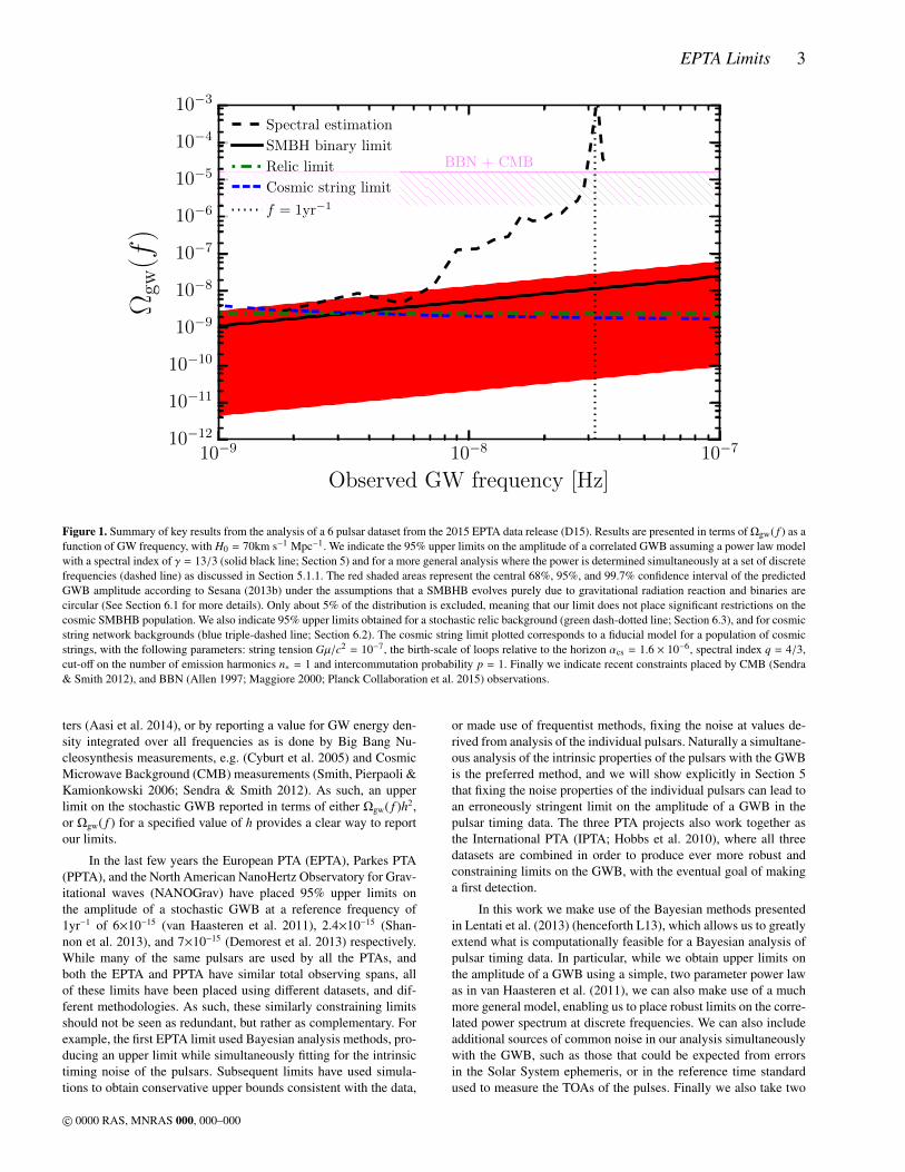
Figure 3. Top: timing residuals as a function of Modified Julian Date (MJD) for the 6 pulsars included in the stochastic GWB analysis presented in thiswork, after the maximum likelihood DM variations signal realisation has been subtracted. From top to bottom these are PSRs: J0613−0200, J1012+5307,J1600−3053, J1713+0747, J1744−1134, and J1909−3744. While the overall timing baseline for this dataset is ∼ 18 yr, only four of the 6 pulsars have datathat extends across the majority of this timespan, and in particular, PSR J1909−3744 contributes only to the latter half of the dataset, significantly reducing ouroverall sensitivity to signals at the lowest frequencies supported by the dataset. Bottom: Frequency coverage for the 6 pulsars included in the stochastic GWBanalysis presented in this work. The order of the pulsars is as in the top plot. Colours indicate observing frequencies < 1000MHz (red crosses), between 1000and 2000 MHz (green circles) and > 2000 MHz (blue squares). In addition to fewer pulsars extending across the full dataset, there is also less multi-frequencycoverage in the early data. This further decreases our sensitivity to a stochastic GWB at the lowest sampled frequencies as the signal becomes highly covariantwith the DM variations for the individual pulsars in the first half of the dataset.

c© 0000 RAS, MNRAS 000, 000–000

EPTA Limits 11

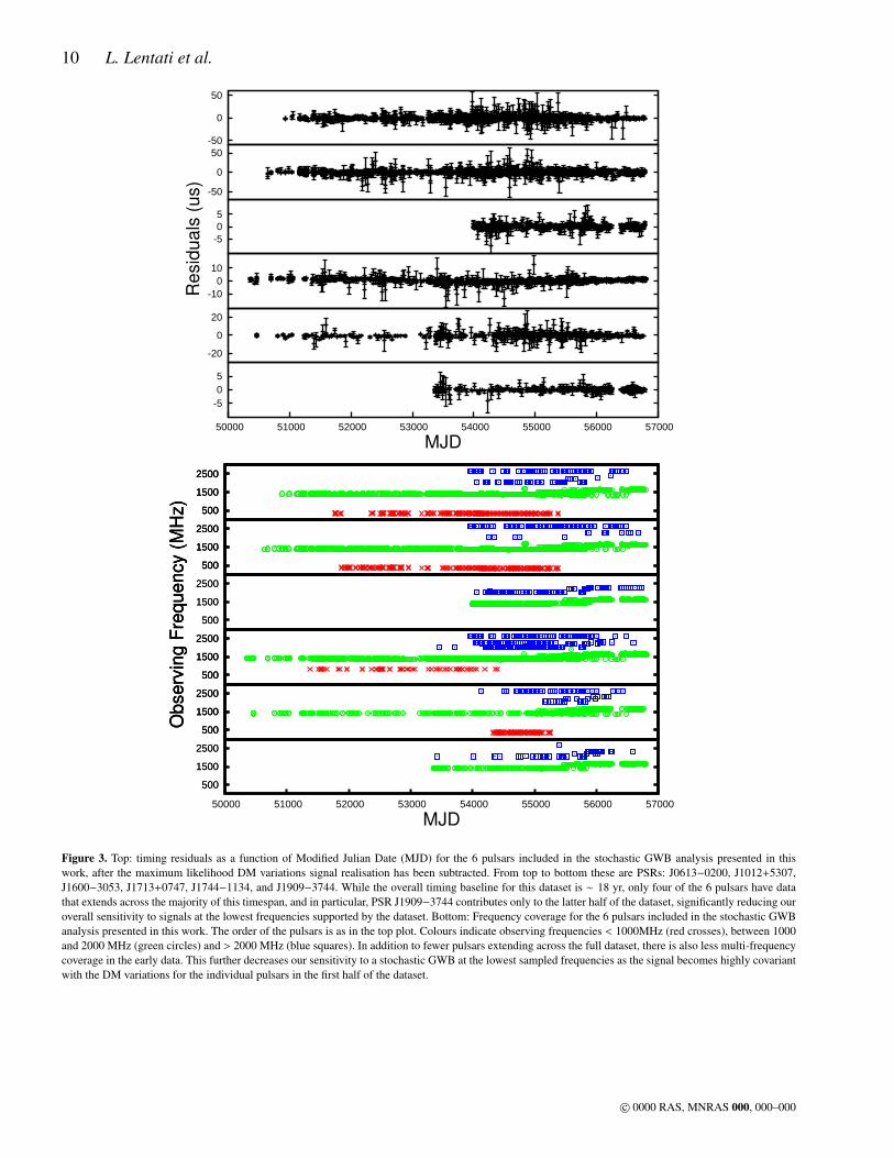
Table 1. Details of the 6 pulsars used for the isotropic stochastic background analysis. Numbers in parentheses correspond to the maximum likelihood valuesfrom the 5-dimensional analysis described in Section 4.

Pulsar J0613−0200 J1012+5307 J1600−3053 J1713+0747 J1744−1134 J1909−3744

Dataspan (yr) 16.05 16.83 7.66 17.66 17.25 9.38Nsys

a 14 15 4 14 9 3σ(µs) b 1.691 1.610 0.563 0.679 0.801 0.131

Log10 ASN -13.58 ± 0.40 (-13.41) -13.05 ± 0.09 (-13.04) -13.71 ± 0.54 (-13.42) -14.31 ± 0.46 (-14.20) -13.63 ± 0.27 (-13.60) -14.22 ± 0.42 (-13.98)γSN 2.50 ± 0.99 (2.09) 1.56 ± 0.37 (1.56) 1.91 ± 1.05 (1.38) 3.50 ± 1.16 (3.51) 2.21 ± 0.82 (2.16) 2.23 ± 0.89 (2.17)

Log10 ADM -11.61 ± 0.12 (-11.57) -12.25 ± 0.47 (-11.92) -11.75 ± 0.39 (-11.67) -11.97 ± 0.14 (-11.90) -12.19 ± 0.38 (-11.93) -12.76 ± 0.53 (-12.51)γDM 1.36 ± 0.48 (1.11) 1.26 ± 0.97 (0.27) 1.64 ± 0.80 (1.46) 2.03 ± 0.55 (1.82) 1.41 ± 1.09 (0.36) 2.23 ± 1.07 (2.16)

Global EFAC 1.01 ± 0.02 (1.01) 0.98 ± 0.02 (0.98) 1.03 ± 0.04 (1.03) 1.00 ± 0.02 (1.00) 1.01 ± 0.03 (1.00) 1.02 ± 0.04 (1.01)95% upper limit c 9.7 × 10−15 8.3 × 10−15 2.1 × 10−14 4.4 × 10−15 7.0 × 10−15 5.2 × 10−15

a Number of unique observing ‘systems’ that make up the dataset for each pulsar.b Weighted rms for the DM subtracted residuals for each pulsar (D15).c Upper limit obtained from the 5-dimensional analysis described in Section 4.

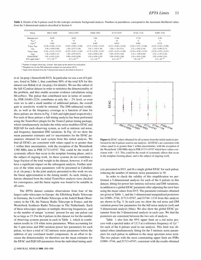
et al. (in prep.) (henceforth D15). In particular we use a set of 6 pul-sars, listed in Table 1, that contribute 90% of the total S/N for thisdataset (see Babak et al. (in prep.) for details). We use this subset ofthe full 42 pulsar dataset in order to minimise the dimensionality ofthe problem, and thus enable accurate evidence calculations usingMultiNest. The pulsar that contributed next in terms of sensitiv-ity, PSR J1640+2224, contributes at only the ∼ 2% level, so evenwere we to add a small number of additional pulsars, the overallgain in sensitivity would be minimal. The DM-subtracted residu-als, as well as the frequency coverage as a function of time forthese pulsars are shown in Fig. 3 (left and right panel respectively).For each of these pulsars a full timing analysis has been performedusing the TempoNest plugin for the Tempo2 pulsar timing package,which simultaneously includes the white noise modifiers EFAC andEQUAD for each observing system, as well as intrinsic red noise,and frequency dependent DM variations. In Fig. (4) we show themean parameter estimates and 1σ uncertainties for the EFAC pa-rameters obtained for each system from this initial analysis. Wefind all EFACs are consistent with values equal to or greater than1 within their uncertainties, with the exception of the Westerbork1380 MHz data in PSR J1713+0747. This could be the result ofsystematic effects that occur in the template forming phase, and isthe subject of ongoing work. As these systems do not contribute alarge fraction of the total weight in the dataset, however, it will nothave a significant impact on the subsequent analysis. Further anal-ysis of the white noise parameters will be presented in Caballeroet al. (in prep.). In the joint analysis presented in this work we usethe linear approximation to the timing model. As such, timing so-lutions obtained from the initial TempoNest analysis were checkedfor convergence, and the linear regime was found to be suitable inall cases.

The EPTA dataset contains observations from four of thelargest radio telescopes in Europe: the Effelsberg Radio Telescopein Germany, the Lovell Radio Telescope at the Jodrell Bank Obser-vatory in the UK, the Nancay Radio Telescope in France, and theWesterbork Synthesis Radio Telescope in The Netherlands. Eachof these telescopes operates at multiple observing frequencies, andso the number of unique ‘systems’ present for any one pulsar canbe as large as 15. For the 6 pulsars in this dataset we list the numberof observing systems present in each in Table 1, which in combi-nation results in 118 white noise parameters. When accounting forthe 4 spin-noise and DM variation power law parameters for eachpulsar, we have a total of 142 intrinsic noise parameters before theaddition of any correlated model components. In an effort to de-crease the dimensionality we therefore use the mean estimates forthe EFAC and EQUAD parameters from the individual timing anal-

0

0.5

1

1.5

2

2.5

J0613-0200

J1012+5307

J1600-3053

J1713+0747

J1744-1134

J1909-3744

EF

AC

Figure 4. EFAC values obtained for all systems from the initial analysis per-formed for the 6 pulsars used in our analysis. All EFACs are consistent withvalues equal to or greater than 1 within uncertainties, with the exception ofthe Westerbork 1380 MHz data in PSR J1713+0747 which have values con-sistent with ∼ 0.5. This could be the result of systematic effects that occurin the template forming phase, and is the subject of ongoing work.

ysis presented in D15, and fit a single global EFAC for each pulsar,reducing the number of intrinsic noise parameters to 30.

In order to check the validity of this simplification we per-formed a 5-dimensional analysis for each of the 6 pulsars in thisdataset, fitting for power law intrinsic red noise and DM variations,in addition to a global EFAC parameter after adjusting the error barsusing the mean values from D15. The parameter estimates obtainedare given in Table 1, and the 1-dimensional marginalised posteriorsfor J1909−3744, J1713+0747, and J1744−1134 from this analysisare shown in Fig. 5. In each case we show the red noise and DMvariation power law parameters for the full noise analysis (red) and5-dimensional analysis (blue). We also show the global EFAC pa-rameter from the 5-dimensional analysis in each case. We find theposteriors are consistent between the two sets of analysis.

Table 1 also lists the 95% upper limit on a red noise pro-cess with a spectral index of 13/3 at a reference frequency of 1yr−1

for each of the 6 pulsars used in our analysis. This limit was ob-tained when simultaneously fitting for the 5 intrinsic noise param-eters for each pulsar in addition to the steep spectrum noise term.The two pulsars with the most constraining upper limit are PSRsJ1909−3744, and J1713+0747, consistent with the results obtained

c© 0000 RAS, MNRAS 000, 000–000

12 L. Lentati et al.

0.9 1 1.1

J1909-3744 EFAC

0.94 0.98 1.02 1.06

J1713+0747 EFAC

0.9 0.95 1 1.05 1.1 1.15

J1744-1134 EFAC

-16.5 -15.5 -14.5

J1909-3744 Log10[ASN]

-16.5 -16 -15.5 -15 -14.5 -14 -13.5

J1713+0747 Log10[ASN]

-14.7 -14.3 -13.9 -13.5 -13.1

J1744-1134 Log10[ASN]

0 1 2 3 4 5 6 7

J1909-3744 γSN

0 1 2 3 4 5 6 7

J1713+0747 γSN

0 1 2 3 4 5 6

J1744-1134 γSN

-15.5 -14.5 -13.5 -12.5

J1909-3744 Log10[ADM]

-13.2 -12.8 -12.4 -12

J1713+0747 Log10[ADM]

-15 -14.5 -14 -13.5 -13 -12.5 -12 -11.5

J1744-1134 Log10[ADM]

0 1 2 3 4 5 6 7

J1909-3744 γDM

1.5 2.5 3.5 4.5

J1713+0747 γDM

0 1 2 3 4 5 6 7

J1744-1134 γDM

Figure 5. Comparison of the 1-dimensional marginalised posterior probability distributions for PSRs (left to right) J1909−3744, J1713+0747, and J1744−1134.The y-axis in all plots represents probability. In each case we show the spin-noise and DM variation power law parameters for the full noise analysis (red solidlines) and 5-dimensional analysis where the TOA error bars have been pre scaled by the mean value of the EFAC/EQUAD parameters for each pulsar backend(blue dashed lines). In both cases parameter estimates have been obtained using a uniform prior on the amplitude of the spin-noise and DM variations powerlaw models. We also show the global EFAC parameters from the 5-dimensional analysis in each case. We find the posteriors are consistent between the twosets of analysis.

c© 0000 RAS, MNRAS 000, 000–000

EPTA Limits 13

Table 3. 95% upper limits on the amplitude of an isotropic stochastic GWBobtained for different models at a reference frequency of 1yr−1.

Model 95% upper limit(×10−15)

Bayesian Analysis

Fixed Noise - Fixed Spectral Index 1.7Varying Noise - Fixed Spectral Index 3.0Additional Common Signals - Fixed Spectral Index 3.0

Fixed Noise - Varying Spectral Index 8.0Varying Noise - Varying Spectral Index 13Additional Common Signals - Varying Spectral Index 13

Frequentist Analysis

Fixed Noise - Fixed Spectral Index 2.1

Simulations - Varying Spectral Index

White Noise Only 4.3White and intrinsic spin-noise 7.2White and intrinsic spin-noise and DM variations 12

Table 4. 95% upper limits obtained for common noise terms at a referencefrequency of 1yr−1.

Model 95% upper limit(×10−15)

Additional Common Signals - Varying Spectral Index

ACN 13Aclk 11Aeph (x) 65Aeph (y) 14Aeph (z) 25

in Babak et al. (in prep.), with values of ≈ 5×10−15, and ≈ 4×10−15

respectively.

5 RESULTS

5.1 Limits on an Isotropic Stochastic GWB

5.1.1 Bayesian approach

In Table 2 we list the complete set of free parameters that we in-clude in the different models used in the analysis presented in thissection, along with the prior ranges used for those parameters.

When parameterising the stochastic GWB using the power lawmodel in Eq. (3), we run two parallel sets of analyses: in the first setwe fix γ = 13/3, consistent with a stochastic GWB dominated bySMBHBs; in the second set we allow γ to vary freely within a priorrange of [0,7]. In both cases we consider three different models:

(i) with the intrinsic timing noise for each pulsar fixed at themaximum likelihood values given in Table 1;

(ii) with the intrinsic timing noise for each pulsar allowed tovary;

(iii) as in (ii), but including additional common uncorrelated red

−15.5 −15 −14.5 −14

1 2 3 4 5γ

Log10

[ A ]

γ

−15.5 −15 −14.5 −14

1

2

3

4

5

EPTA Dataset

Figure 7. One and two-dimensional marginalised posterior parameter es-timates for the amplitude and spectral index of a correlated GWB in the6 pulsar dataset presented in this paper when varying the intrinsic noiseparameters for each pulsar. The amplitude and spectral index are highlycorrelated, resulting in a significantly higher upper limit when allowing thespectral index to vary, as opposed to fixing it at a value of 13/3.

noise, a clock error, and errors in the Solar System ephemeris asdiscussed in Section 2.6.

The 95% upper limits for the amplitude of an isotropicstochastic GWB in the six different models are listed in Table 3.In Table 4 we then list the 95% upper limits for the additional com-mon noise terms that were included in model (iii), when allowingthe spectral indicies to vary. All upper limits in this section are re-ported at a reference frequency of 1yr−1.

The one-dimensional marginalised posteriors for the ampli-tude of the GWB for each of these models are shown in Fig. 6.We find that in both the fixed, and varying spectral index modelfor the GWB, limits placed under the assumption of fixed intrinsictiming noise are erroneously more stringent than when the noise isallowed to vary, by a factor ∼ 1.8 and ∼ 1.6 respectively. This isa direct result of using values for the intrinsic noise that have beenobtained from analysis of the individual pulsars, in which the redspin-noise signal, and any potential GWB signal will be completelycovariant. The natural consequence is that fixing the properties ofthe intrinsic noise to those obtained from the single pulsar analysiswill always push the upper limit for the GWB lower in a subsequentjoint analysis.

Both of the most recent isotropic GWB limits from pulsar tim-ing have been set using frequentist techniques, either by performinga fixed noise analysis (Demorest et al. 2013), or using simulations(Shannon et al. 2013), obtaining 95% upper limits of 7 × 10−15 and2.4 × 10−15 respectively. In both cases, therefore, the analysis per-formed was fundamentally different to the Bayesian approach pre-sented in this work. As such it is difficult to compare our resultsdirectly, or to ascertain the effect of fixing the intrinsic noise pa-rameters on limits obtained using those methods.

The most recent limit placed when allowing the intrinsic noiseparameters of the pulsars to vary is given by van Haasteren et al.(2011), in which a 95% upper limit of A = 6 × 10−15 was ob-tained at a spectral index of 13/3. Our model (ii) is most com-

c© 0000 RAS, MNRAS 000, 000–000

14 L. Lentati et al.

Table 2. Free parameters and prior ranges used in the Bayesian analysis.

Parameter Description Prior range

White noiseα Global EFAC uniform in [0.5 , 1.5] 1 parameter per pulsar (total 6)

Spin-noiseASN Spin-noise power law amplitude uniform in [10−20 , 10−10] 1 parameter per pulsar (total 6)γSN Spin-noise power law spectral index uniform in [0, 7] 1 parameter per pulsar (total 6)

DM variationsADM DM variations power law amplitude uniform in [10−20 , 10−10] 1 parameter per pulsar (total 6)γDM DM variations power law spectral index uniform in [0, 7] 1 parameter per pulsar (total 6)

Common noiseACN Uncorrelated common noise power law amplitude uniform in [10−20 , 10−10] 1 parameter for the arrayγCN Uncorrelated common noise power law spectral index uniform in [0, 7] 1 parameter for the arrayAclk Clock error power law amplitude uniform in [10−20 , 10−10] 1 parameter for the arrayγclk Clock error power law spectral index uniform in [0, 7] 1 parameter for the arrayAeph Solar System ephemeris error power law amplitude uniform in [10−20 , 10−10] 3 parameters for the array (x, y, z)γeph Solar System ephemeris error power law spectral index uniform in [0, 7] 3 parameters for the array (x, y, z)

Stochastic GWBA GWB power law amplitude uniform in [10−20 , 10−10] 1 parameter for the arrayγ GWB power law spectral index uniform in [0, 7] 1 parameter for the arrayρi GWB power spectrum coefficient at frequency i/T uniform in [10−20 , 100] 1 parameter for the array per frequency in

unparameterised GWB power spectrum model (total 20)

Stochastic background angular correlation functionc1...4 Chebyshev polynomial coefficient uniform in [−1, 1] see Eq. (36)ΓIJ Correlation coefficient between pulsars (I,J) uniform in [−1, 1] 1 parameter for the array per unique pulsar pair (total 15)

1e-15 2e-15 3e-15 4e-15 5e-15

Pro

ba

bili

ty

GWB Power Law Amplitude

5e-15 1e-14 1.5e-14 2e-14

Pro

ba

bili

ty

GWB Power Law Amplitude

Figure 6. One-dimensional marginalised posterior parameter estimates for the amplitude of a correlated GWB in the 6 pulsar dataset presented in this paperwhen: (left) Fixing the spectral index of the power law to a value of 13/3, consistent with a background dominated by a population of SMBHB, and (right) whenmarginalising over the spectral index given a prior range of [0,7]. In each case we show the posterior given: (red solid line) Fixed intrinsic noise parameters foreach pulsar, where the values of the parameters are given by the maximum likelihood estimates listed in Table 1, (black dotted line) varying noise parametersfor each pulsar, and (magenta dashed line) varying noise parameters for each pulsar, and additionally including a common uncorrelated red noise process,clock errors, and errors in the Solar System ephemeris in the model. Vertical lines in each case represent the 95% upper limits for each model.

parable to this analysis, in which we obtain a 95% upper limit ofA = 3 × 10−15, an improvement of a factor of two. This translatesinto a limit on Ωgw( f )h2 = 1.1 × 10−9 at 2.8 nHz. We confirm thisresult by analysing the 2015 EPTA dataset with model (ii) using anindependent code2, which makes use of the PAL, parallel-temperedadaptive MCMC sampler3 which explores the parameter space in afundamentally different way to MultiNest, and obtain a consistent95% upper limit.

Finally for model (iii) when including additional common or

2 https://github.com/stevertaylor/NX013 https://github.com/jellis18/PAL2

correlated terms in the analysis we find the extra parameters havea negligible impact on our sensitivity, with consistent upper limitsobtained in both the fixed and varying spectral index models.

We find the upper limits for the uncorrelated common rednoise model to be consistent with those obtained for the GWB,however we find the upper limit for the clock error signal tobe slightly lower, with Aclk < 1.1 × 10−14 compared to ACN <

1.3 × 10−14. This is to be expected however, as the clock is han-dled coherently across all pulsars, whereas the GWB and commonuncorrelated red noise signals are handled incoherently, as such wehave greater sensitivity when searching for the clock signal and ob-tain a correspondingly lower limit for the amplitude.

c© 0000 RAS, MNRAS 000, 000–000

EPTA Limits 15

−17.5 −16.5 −15.5 −14.5

1 3 5γLog

10 [ A ]

γ

−17.5 −16.5 −15.5 −14.5

1

3

5

Simulation 1

−16 −15 −14

2 4 6γ

Log10

[ A ]

γ

−16 −15 −14

2

4

6

Simulation 2

−15.5 −15 −14.5 −14

2 3 4 5 6γ

Log10

[ A ]

γ

−15.5 −15 −14.5 −14

2

3

4

5

6

Simulation 3

Figure 8. One and two-dimensional marginalised posterior parameter esti-mates for the amplitude and spectral index of a correlated GWB in 3 sim-ulated datasets, including (Top) White noise only, (Middle) White and in-trinsic spin-noise only, and (Bottom) White noise, intrinsic spin-noise, anddispersion measure variations. In each case we use the TOAs from the 6pulsars used in the GWB analysis presented in this work, and use the maxi-mum likelihood noise parameters from Table 1 when constructing the sim-ulations. The upper limits obtained in each case are 4.3×10−15, 7.2×10−15,and 1.2 × 10−14. We find both the upper limit, and the form of the posteriorto be consistent between the third simulation and the real dataset. In bothcases we are simply recovering our uniform prior on the amplitude of theGWB signal at small amplitudes, before the data begins to place constraintson the upper limit at large amplitudes.

The limits on the different errors originating in the Solar Sys-tem emphemeris can be understood given the components of theunit vector from the SSB toward the two pulsars that contributemost to our analysis, PSRs J1713+0747 and J1909−3744, whichare given by (−0.20,−0.97,+0.14) and (+0.24,−0.75,−0.61) re-spectively. Both PSRs J1909−3744 and J1713+0747 contributevery little to the constraints on the ephemeris in the x direction, andso here we see the greatest degradation in the limit on the ampli-tude, while in the y direction PSR J1713+0747 contributes almostfully and so the limit we obtain is only slightly worse than thatobtained for the GWB and uncorrelated common noise terms.

We consider model (iii) to be the most robust analysis pre-sented in this paper, and so conclude that the 95% upper limit pro-vided by our dataset on a power law GWB is A < 3.0 × 10−15 atγ = 13/3 , and A < 1.3 × 10−14 when marginalising over spectralindex.

That the upper limit is considerably higher in the varying spec-tral index model can be understood from the two-dimensional pos-terior distribution for A and γ in Fig. 7. Here we see the clear cor-relation between the two quantities; as we will see below, our PTAis most sensitive at frequencies 1 yr−1, meaning that for a singlepower-law spectrum, the flatter the spectral index, the less stringentthe limit on A.

As a consistency check on this result we perform a set of threesimulations using the sampled time stamps present in the actual 6pulsar dataset. In the first simulation we include only a white noisecomponent with an amplitude determined using the TOA uncer-tanties from the real dataset. In the second simulation we then addan intrinsic spin-noise component, with amplitudes and spectral in-dices equal to the maximum likelihood values presented in Table1. Finally in the third simulation we also include DM variations,where as with the intrinsic spin-noise we use the maximum likeli-hood values in Table 1 to set the amplitudes and spectral indices.Critically in all the simulations we include no correlated GWBterm, and so in each case we expect to recover only our uniformprior on the amplitude of the GWB included in our model.

The one and two-dimensional marginalised posterior parame-ter estimates for the amplitude and spectral index of the GWB fromeach of the three simulations are shown in Fig. 8. We obtain upperlimits of 4.3 × 10−15, 7.2 × 10−15, and 1.2 × 10−14 in each case re-spectively. In all the one-dimensional posterior distributions for theamplitude of the signal we are simply recovering our prior, suchthat the probability is proportional to the amplitude of the signalbelow some limit set by the data. In the case of the third simula-tion, which is most similar to the real dataset, both the upper limit,and the form of the posterior is consistent with the results presentedin Fig. 7 and Table 3.

In Fig. 9, we show the 95% upper limits from a power spec-trum analysis that does not assume a power law model, but allowsthe power at each frequency included in the model to vary sep-arately. We perform this analysis separately both for a correlatedGWB (red points), and uncorrelated common red noise process(blue points) while varying the intrinsic noise parameters for eachpulsar, however we do not include any additional common terms.The upper limit obtained from the equivalent power law analysisof the GWB at a spectral index of 13/3 of 3 × 10−15 is overplot-ted as a straight line. Frequencies were included from 1/T up to20/T , with T = 17.66 yr, beyond which we do not expect the datato provide significant constraints on a steep red noise process. Wefind that our limit at a spectral index of 13/3 is most heavily con-strained by the 3/T term, corresponding to f ≈ 5× 10−9Hz. This islikely a combination of the lack of multifrequency data in the early

c© 0000 RAS, MNRAS 000, 000–000

16 L. Lentati et al.

0 1 2 3 4 5 6 7γ ≡ 3− 2α

10−17

10−16

10−15

10−14

10−13

A

Optimal-statistic bounds

95.0% upper-limit

90.0% upper-limit

0 20 40 60 80 100 120 140 160 180

Pulsar angular separation [degrees]

−4

−3

−2

−1

0

1

2

3

Cro

ssp

ower

×10−28 Cross-power measurements

Figure 12. (left) Frequentist upper-limits on the strain amplitude of the stochastic GWB obtained via the optimal-statistic for our 6 pulsar dataset. Red linesindicate 90% and 95% upper-limits at the fiducial slope of the strain-spectrum of −2/3, which corresponds to a slope of the residual PSD of −13/3. (right)The individual cross-power values are shown for our 6 pulsar dataset. All values are consistent with zero cross-correlation.

-15

-14

-13

-12

-1.4 -1 -0.6 -0.2 0.2

Lo

g10[P

ow

er

(s2)]

Log10[Frequency (years-1

)]

Figure 9. (Top) 95% upper limits from an unparameterised power spectrumanalysis for a correlated GWB (red points), and uncorrelated common rednoise process (blue points) for the 6 pulsar dataset described in Section 4obtained while varying the intrinsic noise parameters for each pulsar. Theupper limit obtained from a power law analysis of the GWB at a spectralindex of 13/3 of 3 × 10−15 is overplotted as a straight line. Frequencieswere included from 1/T up to 20/T , with T = 17.66 yr. Beyond thesefrequencies the data provides increasingly poorer constraints on a steep rednoise process, and so we do not consider higher frequency terms in ourmodel. Both the correlated and uncorrelated power spectrum are completelyconsistent with one another at all frequencies. The difference in the logEvidence between the correlated and uncorrelated models was 0.2 ± 0.3,indicating no support for the presence of a correlated signal in the dataset.

data for PSR J1713+0747 as shown in Fig. 3, which significantlyimpacts our ability to disentangle DM variations from frequency-independent red noise at the lowest frequencies, and that our PSRJ1909−3744 dataset is only ∼ 9 yr in length. Despite these limi-tations, the long timing baseline of the EPTA dataset used in thiswork is still critical for placing limits on the lowest frequencies in

5e-15 1e-14 1.5e-14 2e-14

Pro

ba

bili

ty

Power Law Amplitude

Figure 10. One-dimensional marginalised posterior parameter estimates forthe amplitude of a correlated GWB (red solid line) and an uncorrelated com-mon red noise model (blue dashed line) in the 6 pulsar dataset presented inthis paper when marginalising over the spectral index given a prior rangeof [0,7]. Posteriors were obtained when varying the intrinsic noise param-eters, and including only either the GWB, or common uncorrelated terms.We find the upper limits to be completely consistent with one another, andobtain a change in the log evidence of −1.0 ± 0.5 for the GWB model overthe uncorrelated common red noise model, suggesting no strong support foreither.

our analysis. Both the correlated and uncorrelated power spectrumare completely consistent with one another at all frequencies. Thedifference in the log Evidence between the correlated and uncorre-lated models was 0.2 ± 0.3, indicating no support for the presenceof a correlated signal in the dataset.

In Fig. 10 we further assess the impact of including, or not,the Hellings-Downs correlation on the upper limit obtained in ourpower law model (ii) for the varying spectral index case. We showthe one-dimensional marginalised posterior for both the amplitudeof the GWB, which includes the correlation between pulsars (redsolid line), and for the amplitude of an uncorrelated common rednoise power law process (blue dashed line). We find the upper limitsto be completely consistent with one another, and obtain a change

c© 0000 RAS, MNRAS 000, 000–000

EPTA Limits 17

Figure 11. The recovered correlation between pulsars as a function of an-gular separation on the sky for a power law noise process. The red and bluelines represent the 68% and 95% confidence intervals for the correlationfunction when modelled by the lowest 4 Chebyshev polynomials, whilethe individual points are the mean correlation coefficient with 1σ uncer-tainty for each pulsar pair when fitting without assuming a smooth model.The Hellings-Downs correlation is represented by the dotted line. For bothmodels the correlation of a common power law model between pulsars isconsistent with effectively all possible values (the range [-1,1]).

in the log evidence of −1.0±0.5 for the GWB model over the uncor-related common red noise model, indicating no strong support foreither model in the data. We confirm this result by obtaining con-straints on the correlation between pulsars as a function of angularseparation for a common power law model, where the amplitudeand spectral index of the power law are free to vary, and we fit si-multaneously for the intrinsic noise parameters for the individualpulsars. We fit for the correlation using the two methods describedin Section 2.7, using either the four lowest order Chebyshev poly-nomials, or fitting for the correlation coefficient directly. In Fig.11 the red and blue lines represent the 68% and 95% confidenceintervals for the correlation function when modelled by the low-est 4 Chebyshev polynomials, while the individual points are themean correlation coefficient with 1σ uncertainty for each pulsarpair when fitting directly. In both cases the correlation is consistentwith effectively all possible values (the range [-1,1]).

5.1.2 Frequentist approach

Applying the optimal-statistic introduced in Section 3.2 to our re-duced 6 pulsar dataset, and testing for a strain-spectrum slope of−2/3, gives A2 = (−2.86 ± 4.29) × 10−30, with an associatedS/N = −0.67. This is clearly a non-detection, however the 95%upper-limit on A is 2.05 × 10−15, which is more constraining thanthe best published limit of Shannon et al. (2013), and is consistentwith the fixed noise Bayesian limit of 1.7 × 10−15. The optimal-statistic limits as a function of slope are shown in the left panel ofFig. 12, with limits at the fiducial slope value marked in red.

The computed cross-power values for our 6 pulsar dataset areshown in the right panel of Fig. 12, and are all consistent with zerocorrelation, as expected.

6 DISCUSSION

6.1 Implications for SMBHB astrophysics

As discused previously, the most promising astrophysical source ofGWs in the nHz regime relevant to PTA observations is a cosmo-logical population of adiabatically in-spiralling SMBHBs.

In this section we will consider the implications of the upper-limit obtained in Section 5 on the gravitational-wave signal formodels of astrophysical populations of SMBHBs. If we assumethat a SMBHB evolves purely due to gravitational radiation reac-tion, and that all SMBHBs are in circular orbits – we will returnto these assumptions at the end of the section – the characteristicamplitude, Eq. (2), is given by:

h2c( f ) =

4 f −4/3

3π1/3

∫ ∫dzdM

d2ndzdM

1(1 + z)1/3M

5/3, (53)

so that

A =2 f −2/3

1yr√

3π1/6

[∫ ∫dzdM

d2ndzdM

1(1 + z)1/3M

5/3]1/2

. (54)

A limit on the amplitude A, as given by Eq. (53) therefore placesconstraints on d2n/(dzdM), i.e., the number density of SMBHBmergers per unit redshift and unit chirp mass across cosmic his-tory. Although the dominant contribution to the signal comes fromrelatively massive (M > 108 M), low redshift (z < 2) systems(Sesana, Vecchio & Colacino 2008), their merger rate is still poorlyconstrained, resulting in a fairly wide range of possible signalamplitudes. Sesana, Vecchio & Colacino (2008) exploited semi-analytical merger trees from Volonteri, Haardt & Madau (2003)to estimate a plausible range for the amplitude of a GWB of5× 10−16 < A < 3× 10−15. Merger rates extracted from cosmologi-cal simulations like the Millennium (Springel et al. 2005) and Mas-sive Black (Khandai et al. 2014) simulations, coupled with differentprescriptions for the SMBH-galaxy relation results in a compatablerange of 4 × 10−16 < A < 2 × 10−15 (Sesana, Vecchio & Volonteri2009; Ravi et al. 2012). Recently, Sesana (2013b) constrained theexpected range of A by building a set of phenomenological modelsbased on the observed properties of interacting galaxies. Thousandsof models fulfilling all relevant observational constraints were as-sembled by combining different estimates of the galaxy mass func-tion, pair fractions, estimated merger times and galaxy-SMBH re-lations. The central 90% of the probability distribution function(PDF) in the amplitude A lies in the range 3×10−16 < A < 3×10−15,as shown in the right panel of Fig. 13. A similar approach was em-ployed by Ravi et al. (2014a), yielding consistent results.

In Fig. 13 we compare the expected range in hc predicted bythe phenomenological models presented in Sesana (2013b) to the95% upper limit obtained in Section 5.1. Shaded areas representthe central 68%, 95%, 99.7% and 100% confidence intervals forthe predicted signal. The red curve is derived by converting the95% limit on the unparametrised power spectrum shown in Fig. 9into hc as

hc = (power × 12π2 f 3T )1/2, (55)

where T is the total observation time. Eq. (55) can be calculateddirectly from Eq. (3) by noting that the power at each frequencyis the integral of S ( f ) over a frequency bin ∆ f = 1/T . Fig. 13 in-structively shows how the limit on A that is usually quoted in theliterature is extrapolated from the actual sensitivity of the PTA. Ourdataset is most sensitive at f ≈ 5×10−9Hz, where the 95% limit onhc is ∼ 1.1× 10−14. This is then extrapolated to f = 1yr−1 assuminga f −2/3 power-law, to get a 95% upper limit of A = 3.0 × 10−15.

c© 0000 RAS, MNRAS 000, 000–000

18 L. Lentati et al.

The right panel of Fig. 13 shows the probability distribution of Ainferred from the theoretical models of Sesana (2013b) togetherwith the region excluded at 95% confidence by our analysis. Onlyabout 5% of the distribution is excluded, meaning that our limitdoes not place severe restrictions on the cosmic SMBHB popu-lation. Note that A values obtained from merger trees and cos-mological simulations quoted above are generally in the range4 × 10−16 < A < 3 × 10−15, and therefore also consistent with thislimit.

We caution that Fig. 13 shows the expected range of the GWsignal given circular GW driven SMBHBs, with negligible cou-pling to the environment. It has been shown (see, e.g. Enoki & Na-gashima 2007; Kocsis & Sesana 2011; Sesana 2013a; McWilliams,Ostriker & Pretorius 2014; Ravi et al. 2014b) that both high ec-centricities and strong environmental coupling might cause a sig-nificant suppression of the GW signal at f < 10−8Hz. If this isthe case, our 1.1 × 10−14 limit at f ≈ 5 × 10−9Hz cannot be ex-trapolated to f = 1yr−1 using a simple power-law model. Even amuch more stringent limit obtained at such low frequencies mightnot have significant implications for the cosmic SMBHB mergerrate, because the suppression at low frequencies would invalidatethe f −2/3 extrapolation to higher frequencies (see Fig. 2 in Sesana2013a). Since the detailed dynamical evolution of SMBHBs cou-pled with their environment is still poorly understood, current PTAlimits do not allow us to formulate strong astrophysical statementsabout the cosmological population of SMBHBs.

6.2 Limits on the cosmic (super)string tension

The limits computed in Section 5.1 can be converted into upperlimits on the linear energy density of a cosmic (super)string net-work, µ, or tension in the Nambu-Goto approximation, usually de-scribed by the dimensionless quantity Gµ/c2, where G is New-ton’s constant and c the speed of light. Field theory cosmic strings(Kibble 1976; Jeannerot, Rocher & Sakellariadou 2003), are one-dimensional topological defects, relics of an early, more symmetricstate of the Universe, created through the mechanism of sponta-neous symmetry breaking during the various phase transitions thatthe early Universe underwent. Their formation is a generic propertyof supersymmetric hybrid inflation scenarios (Jeannerot, Rocher &Sakellariadou 2003), whereas the creation of their superstring the-ory counterparts, usually referred to as cosmic superstrings, are alsoa natural by-product of brane inflation scenarios (e.g. Sarangi &Tye 2002; Jones, Stoica & Tye 2003).

A cosmic string network consists of “infinite” (larger than theparticle horizon) strings and cosmic string loops. A cosmic stringnetwork grows along the expansion of the Universe and is expectedto settle in a scaling regime, were all the fundamental propertiesof the network grow proportionally with cosmic time, somethingachieved with the creation of loops; the main energy loss mecha-nism of the network. When two cosmic strings intersect, they “in-tercommute” (exchange partners) with a characteristic probability,and form loops. Cosmic string loops, once created, oscillate anddecay emitting all of their energy in various forms of radiation,with the dominant form thought to be GWs (Vilenkin 1981). Thestochastic GWB created by a cosmic string network is broadband(from ∼10−16 Hz, to higher than 109 Hz, depending on the size of theloops created), a characteristic feature of primordial GW sources,and is potentially detectable by any present or future GW detector.The cosmic string GW spectrum consists of a flat part at high fre-quencies, originating from loops decaying in the radiation era, anda broad peak at lower frequencies originating from loops decaying

10−9 10−8 10−7

Observed GW Frequency [Hz]

10−16

10−15

10−14

10−13

10−12

Ch

ara

cter

isti

cA

mp

litu

de

0 0.1

PDF

Figure 13. Comparison between the expected GWB amplitude from a cos-mological population of SMBHBs and the 95% upper limit obtained withour PTA experiment. Shaded areas represent the central 68%, 95%, 99.7%and 100% confidence interval of the predicted signal according to Sesana(2013b), whereas the red curve is the 95% upper limit presented in thispaper, obtained by converting the unparametrised power spectrum shownin Fig. 9 to characteristic amplitude. The black triangle is the extrapolated95% upper limit on A at f = 1yr−1. The right panel shows the PDF of thepredicted hc at f = 1yr−1, and the shaded area marks the region excluded at95% confidence by our limit (less than 5% of the distribution).

in the matter era. PTAs are in the privileged position to typicallyprobe the GW emission originating from loops decaying either inthe matter era or in the radiation-to-matter era transition, makingthem excellent instruments to detect the stochastic GWB of a cos-mic string network. In the case of a non-detection, the upper limitson the GWB can be used to constrain the energy scale of cosmicstrings.

There are numerous investigations on the cosmic string GWBin the literature (e.g. Damour & Vilenkin 2005; Olmez, Mandic &Siemens 2010; Depies & Hogan 2007), depending on various as-sumptions concerning the GW emission mechanisms and the com-putation of the loop number density. The cosmic string GWB spec-tra used in this paper are those computed in Sanidas, Battye & Stap-pers (2013), which are based on an updated version of the mod-elling presented in Sanidas, Battye & Stappers (2012). The maindifference of these two investigations is the inclusion of the effectsof massive particle annihilation, which reduces the amplitude ofthe spectrum at higher frequencies. Both investigations, however,do not make any assumptions about the values of the fundamen-tal model parameters used to compute the GW spectrum, grant-ing characteristic robustness to the results presented here. Sanidas,Battye & Stappers (2012) presented a generic way to compute theGWB based on the widely accepted one-scale model for cosmic

c© 0000 RAS, MNRAS 000, 000–000

EPTA Limits 19

hc

−16

−15.5

−15

−14.5

−14

−13.5

γ01234567

log 1

0 Ωh2

−12

−11

−10

−9

−8

−7

−6

Ω spectral slope−2 −1 0 1 2 3 4 5

Figure 14. The 95% confidence upper limits on the amplitude of anisotropic, stochastic GWB as a function of the local spectral index at thefrequency of 1 yr−1, imposed by models (ii) (dashed black) and (iii) (solidred) of Section 5.1. The limits are expressed in terms of the strain of theGWB, hc, and the dimensionless spectral energy density of GWs, Ωh2,where H0 = 100h km s−1 Mpc−1, as a function of their respective spectralindices.

strings. The basic parameters of this model are the string tensionGµ/c2, the birth-scale of loops relative to the horizon, αcs, andthe intercommutation probability, p. Based on this modelling, andassuming that the cosmic string network maintains a scaling evo-lution along the expansion of the Universe, one can compute theloop number density for all the parameter combinations that createa GWB at the frequency regime probed by PTAs. Additionally, noassumption is made concerning the dominant GW emission mecha-nism from the strings (i.e., kinks or cusps), which is modelled usingtwo additional parameters, a spectral index, q, and a cut-off, n∗, onthe number of emission harmonics n.

In this section we present updated constraints on the cosmicstring tension, for various values of the intercommutation proba-bility, but independent of all the rest model parameters. The GWBupper limits we used are those obtained in the analysis for the mod-els (ii) and (iii) of Section 5.1, where the spectral index γ was afree parameter, as these are presented in Fig. 14. Additionally, weused the GW sensitivity curve in Fig. 13 to investigate tension con-straints across the probed frequency range. In the first case, we usedthe information of both the amplitude and the local spectral indexof the GWB in order to create the tension exclusion curves in thecosmic string model parameter space, whereas in the second casewe used only the amplitude information. In Fig. 15, we presentthe cosmic string tension exclusion curves in the parameter spaceGµ/c2 − αcs accessed by the PTAs, for field theory strings (p = 1).These exclusion curves were constructed from the combination ofthe n∗ = 1 and n∗ = 104 exclusion curves, depending on whichone provided the highest tension value. The limits are provided bythe n∗ = 1 networks in the mid-αcs region (−8 . log10 αcs . −3),whereas in the large (log10 αcs & −3) and small (−8 . log10 αcs)loop regimes, by the n∗ = 104 networks. As discussed in Sanidas,Battye & Stappers (2012), the n∗ = 1 and n∗ = 104 cases will al-ways provide the largest tension values for fixed values of the restcosmic string model parameters. The limits from the n∗ = 1 net-works are independent of the GW emission mechanism since thepower emitted per emission mode is ∝ n−q. For the limits providedby the n∗ = 104 networks, we used a spectral index q = 4/3, cor-

-10 -9 -8 -7 -6 -5 -4 -3 -2 -1-12

-11

-10

-9

-8

-7

-6

log10acs

log 1

0G

mêc

2

Figure 15. Exclusion limits for different cosmic string network configura-tions with the same Ωh2 value at a frequency f = 1 yr−1 in the Gµ/c2 − αcsparameter space, for p = 1. Both the amplitude and spectral slope infor-mation of the GWB limits were used to construct the limits. The dashedblack and solid red curves, are based on the results of models (ii) and (iii)presented in Fig. 14 respectively. In the mid-αcs region, the tension upperlimits are provided by the n∗ = 1 networks, whereas in the regime of largeand small loops, by the n∗ = 104 networks.

responding to cusp emission, which always provides larger tensionvalues than the q = 2 case which corresponds to emission fromkinks. The cosmic string tension upper limit for model (ii), wherethe intrinsic timing noise of each pulsar is allowed to vary, is

Gµ/c2 < 1.2 × 10−7(95% confidence), (56)

whereas the tension upper limit for model (iii) where the commonuncorrelated red noise, clock and Solar System ephemeris errorsare included is

Gµ/c2 < 1.3 × 10−7(95% confidence). (57)

For the particular case of large loop production with α = 0.05,as suggested by the most recent Nambu-Goto cosmic string evolu-tion simulations (Blanco-Pillado, Olum & Shlaer 2011, 2014), weget an upper limit Gµ/c2 < 3.0 × 10−11. The tension constraint thatwas obtained based on that loop number density and the previousEPTA GWB limit was Gµ/c2 < 2.8 × 10−9 (Blanco-Pillado, Olum& Shlaer 2014). Assuming a ∼1.7 times improvement on the valueof the Ωgw used in that work, one would expect approximately aconstraint Gµ/c2 . 9.7 × 10−10. This order of magnitude differ-ence stems mostly from the normalization imposed on the producednumber of loops. Whereas in our model we assume that all of theenergy lost by the cosmic string network in order to attain scal-ing is channeled in loops of just one size, the loop production in(Blanco-Pillado, Olum & Shlaer 2014) takes place on a much widerrange of large loops (wider range of α). The difference in these twoconstraints is expected, since as we have demonstrated in Sanidas,Battye & Stappers (2012), where we also assumed a log-normaldistribution for the loop birth scale, a wider range for the values ofα has as an effect the lowering of the matter era peak GWB ampli-tude and its broadening. However, a direct comparison of these tworesults is not straightforward, not only because of the loop num-

c© 0000 RAS, MNRAS 000, 000–000

20 L. Lentati et al.

Table 5. Upper limits on the cosmic superstring tension Gµ/c2 for p , 1and the two scaling laws proposed in the literature, using the GWB limitsplaced by models (ii) and (iii).

Scenario ii Scenario iiiModel (varying spectral index, (varying spectral index,

varying noise) additional common noise)

Scaling law k=0.6 k=1 k=0.6 k=1

p = 10−1 2.2 × 10−8 1.1 × 10−8 2.4 × 10−8 1.0 × 10−8

p = 10−2 7.3 × 10−9 1.6 × 10−9 6.9 × 10−9 1.5 × 10−9

p = 10−3 2.3 × 10−9 2.8 × 10−10 2.1 × 10−9 2.2 × 10−10

ber density calculation differences, but also due to differences incomputing the stochastic GWB.

Additionally, we computed the tension upper limits in the caseof p , 1. In general, the intercommutation probability for cosmicsuperstrings can acquire values in the range p ∈ [10−3, 1], depend-ing on their nature (F- or D- cosmic superstrings) (Jackson, Jones& Polchinski 2005). The effect of p , 1 is the increase of the am-plitude of the stochastic GWB, without affecting the shape of theGW spectrum, Ωgw ∝ p−k, where k is the dependence of the scalinglaw that describes the effects of the intercommutation probabilityon the energy density of the infinite cosmic strings (ρ∞ ∝ p−k).

There is no general consensus on the value of k, with differ-ent investigations suggesting a value of k = 0.6 (Avgoustidis &Shellard 2005) or k = 1 (Sakellariadou 2005). The reduced inter-commutation probability, has as a result an increased number ofintercommutations in order to maintain the scaling evolution of thenetwork, and therefore, an increased number of loops which giveGWBs of higher amplitude. In Table 5, we present the tension up-per limits for various cosmic superstring configurations, coveringthe whole possible range of p and k values. These upper limits,which are linked with small tension values, are provided by thenetworks with the smallest loop size accessible (αcs ∼ 6 × 10−11;see discussion in Sanidas, Battye & Stappers 2013). In Fig. 16 wepresent a set of such exclusion curves to demonstrate the change inthe shape of the exclusion curves as we probe lower tension val-ues. The exclusion curves in the region Gµ/c2 . 10−10 are alwaysprovided by the n∗ = 104 networks. The apparent discontinuitiesin some of these exclusion curves are a combinatory result of theabrupt local changes in the GWB upper limit curve (more evidentin the slope region [-2,0] for the Ω in Fig. 14), and our require-ment for a matching in the spectral slope of the GWB limit and thespectral slope of the cosmic string GW spectrum at a frequency4

f = 1 yr−1.In Fig. 17, we present the tension upper limits created from

the sensitivity curve of Fig. 13 in the frequency range f ∈ [1.7 ×10−9, 10−8] in the case where p = 1. We did not produce results forthe whole frequency range of Fig. 13, since already for frequen-cies & 7 × 10−9 Hz the tension upper limits are incompatible to thelarge scale structure of the Universe as we observe it (i.e., CMB

4 This has been verified by using smoother GWB sensitivity curves. Theregions of the Gµ/c2 − αcs parameter space where there is also a signifi-cant change in the local spectral slope of the cosmic string GW spectrum,might also create such discontinuities, but such were not observed in thevarious tests we have conducted to investigate this effect. If one neglectsthe requirement for a matching local spectral index, no such artifacts areobserved.

-10 -9 -8 -7 -6 -5 -4 -3 -2 -1-13

-12

-11

-10

-9

-8

-7

-6

log10acs

log 1

0G

mêc

2

Figure 16. Exclusion curves for a set of network configurations with p , 1.With thick lines are the configurations with k = 0.6 and with thin lines theconfigurations with k = 1. We present exclusion curves for p = 0.1 (solidlines), p = 10−2 (short dashed lines) and p = 10−3 (long dashed lines). Thedot-dashed curve is the exclusion curve for p = 1, for reference purposes.For all the results, we used the stochastic GWB limit of model (iii), placedat a frequency f = 1 yr−1.

-8.5 -8

-7

-6.5

-6

-5.5

-5

log10f HHzL

log 1

0G

mêc2

Figure 17. The cosmic string tension upper limits in the case of p = 1,obtained from the sensitivity curve presented in Fig. 13 for a range of theprobed frequencies. For these limits, only the information about the ampli-tude of the GWB has been used. The most stringent constraint is given bythe lowest frequency probed, whereas results for frequencies higher than∼ 10−8, Hz have been omitted, since already for frequencies & 7× 10−9 Hzthe tension upper limits are unphysically high.

anisotropies at large scales and galaxy distribution at small scales).For its computation, we used only the amplitude of the GWB perfrequency bin, making those results less robust than those whichalso incorporate the information of the local GWB spectral index.The most stringent constraint is provided by the lowest frequencyand is Gµ/c2 < 1.1 × 10−7.

Our upper limit on the string tension for Nambu-Goto stringsis slightly better than the one obtained in the extensive analysisperformed by the Planck Collaboration (Planck Collaboration et al.2014) using Planck data only (Gµ/c2 < 1.5 × 10−7), and identical

c© 0000 RAS, MNRAS 000, 000–000

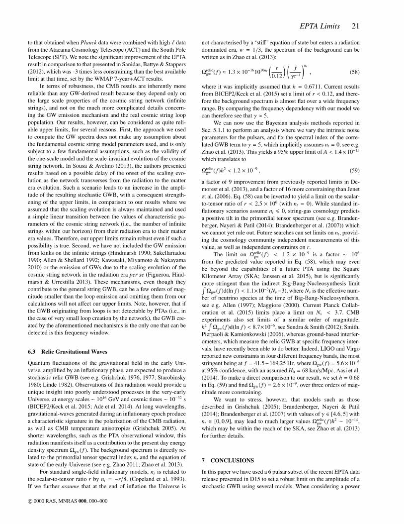
EPTA Limits 21

to that obtained when Planck data were combined with high-` datafrom the Atacama Cosmology Telescope (ACT) and the South PoleTelescope (SPT). We note the significant improvement of the EPTAresult in comparison to that presented in Sanidas, Battye & Stappers(2012), which was ∼3 times less constraining than the best availablelimit at that time, set by the WMAP 7-year+ACT results.

In terms of robustness, the CMB results are inherently morereliable than any GW-derived result because they depend only onthe large scale properties of the cosmic string network (infinitestrings), and not on the much more complicated details concern-ing the GW emission mechanism and the real cosmic string looppopulation. Our results, however, can be considered as quite reli-able upper limits, for several reasons. First, the approach we usedto compute the GW spectra does not make any assumption aboutthe fundamental cosmic string model parameters used, and is onlysubject to a few fundamental assumptions, such as the validity ofthe one-scale model and the scale-invariant evolution of the cosmicstring network. In Sousa & Avelino (2013), the authors presentedresults based on a possible delay of the onset of the scaling evo-lution as the network transverses from the radiation to the matterera evolution. Such a scenario leads to an increase in the ampli-tude of the resulting stochastic GWB, with a consequent strength-ening of the upper limits, in comparison to our results where weassumed that the scaling evolution is always maintained and useda simple linear transition between the values of characteristic pa-rameters of the cosmic string network (i.e., the number of infinitestrings within our horizon) from their radiation era to their matterera values. Therefore, our upper limits remain robust even if such apossibility is true. Second, we have not included the GW emissionfrom kinks on the infinite strings (Hindmarsh 1990; Sakellariadou1990; Allen & Shellard 1992; Kawasaki, Miyamoto & Nakayama2010) or the emission of GWs due to the scaling evolution of thecosmic string network in the radiation era per se (Figueroa, Hind-marsh & Urrestilla 2013). These mechanisms, even though theycontribute to the general string GWB, can be a few orders of mag-nitude smaller than the loop emission and omitting them from ourcalculations will not affect our upper limits. Note, however, that ifthe GWB originating from loops is not detectable by PTAs (i.e., inthe case of very small loop creation by the network), the GWB cre-ated by the aforementioned mechanisms is the only one that can bedetected is this frequency window.

6.3 Relic Gravitational Waves

Quantum fluctuations of the gravitational field in the early Uni-verse, amplified by an inflationary phase, are expected to produce astochastic relic GWB (see e.g. Grishchuk 1976, 1977; Starobinsky1980; Linde 1982). Observations of this radiation would provide aunique insight into poorly understood processes in the very-earlyUniverse, at energy scales ∼ 1016 GeV and cosmic times ∼ 10−32 s(BICEP2/Keck et al. 2015; Ade et al. 2014). At long wavelengths,gravitational-waves generated during an inflationary epoch producea characteristic signature in the polarization of the CMB radiation,as well as CMB temperature anisotropies (Grishchuk 2005). Atshorter wavelengths, such as the PTA observational window, thisradiation manifests itself as a contribution to the present day energydensity spectrum Ωgw( f ). The background spectrum is directly re-lated to the primordial tensor spectral index nt and the equation ofstate of the early-Universe (see e.g. Zhao 2011; Zhao et al. 2013).

For standard single-field inflationary models, nt is related tothe scalar-to-tensor ratio r by nt = −r/8, (Copeland et al. 1993).If we further assume that at the end of inflation the Universe is

not characterised by a ‘stiff’ equation of state but enters a radiationdominated era, w = 1/3, the spectrum of the background can bewritten as in Zhao et al. (2013):

Ωrelicgw ( f ) ≈ 1.3 × 10−161010nt

( r0.12

) (f

yr−1

)nt

, (58)

where it was implicitly assumed that h = 0.6711. Current resultsfrom BICEP2/Keck et al. (2015) set a limit of r < 0.12, and there-fore the background spectrum is almost flat over a wide frequencyrange. By comparing the frequency dependency with our model wecan therefore see that γ ≈ 5.

We can now use the Bayesian analysis methods reported inSec. 5.1.1 to perform an analysis where we vary the intrinsic noiseparameters for the pulsars, and fix the spectral index of the corre-lated GWB term to γ = 5, which implicitly assumes nt = 0, see e.g.Zhao et al. (2013). This yields a 95% upper limit of A < 1.4×10−15

which translates to

Ωrelicgw ( f )h2 < 1.2 × 10−9 , (59)

a factor of 9 improvement from previously reported limits in De-morest et al. (2013), and a factor of 16 more constraining than Jenetet al. (2006). Eq. (58) can be inverted to yield a limit on the scalar-to-tensor ratio of r < 2.5 × 106 (with nt = 0). While standard in-flationary scenarios assume nt 6 0, string-gas cosmology predictsa positive tilt in the primordial tensor spectrum (see e.g. Branden-berger, Nayeri & Patil (2014); Brandenberger et al. (2007)) whichwe cannot yet rule out. Future searches can set limits on nt, provid-ing the cosmology community independent measurements of thisvalue, as well as independent constraints on r.

The limit on Ωrelicgw ( f ) < 1.2 × 10−9 is a factor ∼ 106

from the predicted value reported in Eq. (58), which may evenbe beyond the capabilities of a future PTA using the SquareKilometer Array (SKA; Janssen et al. 2015), but is significantlymore stringent than the indirect Big-Bang-Nucleosynthesis limit∫

Ωgw( f )d(ln f ) < 1.1×10−5(Nν−3), where Nν is the effective num-ber of neutrino species at the time of Big-Bang-Nucleosynthesis,see e.g. Allen (1997); Maggiore (2000). Current Planck Collab-oration et al. (2015) limits place a limit on Nν < 3.7. CMBexperiments also set limits of a similar order of magnitude,h2

∫Ωgw( f )d(ln f ) < 8.7×10−6, see Sendra & Smith (2012); Smith,

Pierpaoli & Kamionkowski (2006), whereas ground-based interfer-ometers, which measure the relic GWB at specific frequency inter-vals, have recently been able to do better. Indeed, LIGO and Virgoreported new constraints in four different frequency bands, the moststringent being at f = 41.5−169.25 Hz, where Ωgw( f ) = 5.6×10−6

at 95% confidence, with an assumed H0 = 68 km/s/Mpc, Aasi et al.(2014). To make a direct comparison to our result, we set h = 0.68in Eq. (59) and find Ωgw( f ) = 2.6× 10−9, over three orders of mag-nitude more constraining.

We want to stress, however, that models such as thosedescribed in Grishchuk (2005); Brandenberger, Nayeri & Patil(2014); Brandenberger et al. (2007) with values of γ ∈ [4.6, 5] withnt ∈ [0, 0.9], may lead to much larger values Ωrelic

gw ( f )h2 ∼ 10−14,which may be within the reach of the SKA, see Zhao et al. (2013)for further details.

7 CONCLUSIONS

In this paper we have used a 6 pulsar subset of the recent EPTA datarelease presented in D15 to set a robust limit on the amplitude of astochastic GWB using several models. When considering a power

c© 0000 RAS, MNRAS 000, 000–000

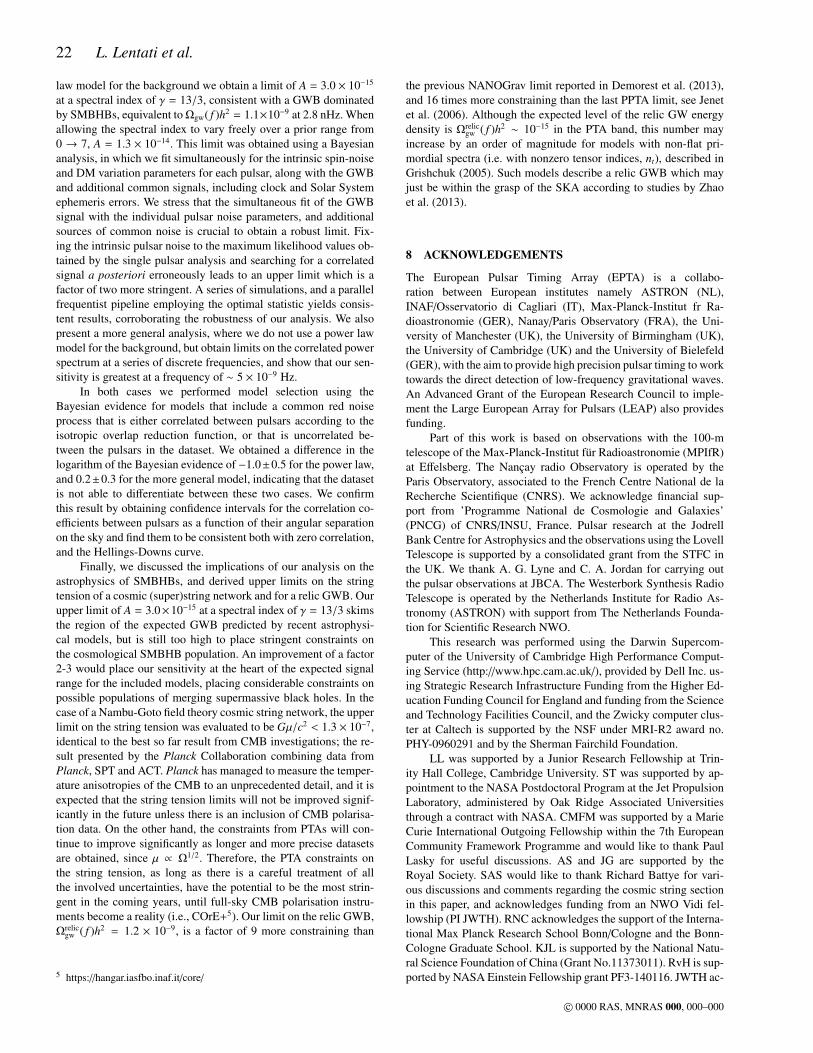
22 L. Lentati et al.

law model for the background we obtain a limit of A = 3.0 × 10−15

at a spectral index of γ = 13/3, consistent with a GWB dominatedby SMBHBs, equivalent to Ωgw( f )h2 = 1.1×10−9 at 2.8 nHz. Whenallowing the spectral index to vary freely over a prior range from0 → 7, A = 1.3 × 10−14. This limit was obtained using a Bayesiananalysis, in which we fit simultaneously for the intrinsic spin-noiseand DM variation parameters for each pulsar, along with the GWBand additional common signals, including clock and Solar Systemephemeris errors. We stress that the simultaneous fit of the GWBsignal with the individual pulsar noise parameters, and additionalsources of common noise is crucial to obtain a robust limit. Fix-ing the intrinsic pulsar noise to the maximum likelihood values ob-tained by the single pulsar analysis and searching for a correlatedsignal a posteriori erroneously leads to an upper limit which is afactor of two more stringent. A series of simulations, and a parallelfrequentist pipeline employing the optimal statistic yields consis-tent results, corroborating the robustness of our analysis. We alsopresent a more general analysis, where we do not use a power lawmodel for the background, but obtain limits on the correlated powerspectrum at a series of discrete frequencies, and show that our sen-sitivity is greatest at a frequency of ∼ 5 × 10−9 Hz.

In both cases we performed model selection using theBayesian evidence for models that include a common red noiseprocess that is either correlated between pulsars according to theisotropic overlap reduction function, or that is uncorrelated be-tween the pulsars in the dataset. We obtained a difference in thelogarithm of the Bayesian evidence of −1.0±0.5 for the power law,and 0.2±0.3 for the more general model, indicating that the datasetis not able to differentiate between these two cases. We confirmthis result by obtaining confidence intervals for the correlation co-efficients between pulsars as a function of their angular separationon the sky and find them to be consistent both with zero correlation,and the Hellings-Downs curve.

Finally, we discussed the implications of our analysis on theastrophysics of SMBHBs, and derived upper limits on the stringtension of a cosmic (super)string network and for a relic GWB. Ourupper limit of A = 3.0×10−15 at a spectral index of γ = 13/3 skimsthe region of the expected GWB predicted by recent astrophysi-cal models, but is still too high to place stringent constraints onthe cosmological SMBHB population. An improvement of a factor2-3 would place our sensitivity at the heart of the expected signalrange for the included models, placing considerable constraints onpossible populations of merging supermassive black holes. In thecase of a Nambu-Goto field theory cosmic string network, the upperlimit on the string tension was evaluated to be Gµ/c2 < 1.3 × 10−7,identical to the best so far result from CMB investigations; the re-sult presented by the Planck Collaboration combining data fromPlanck, SPT and ACT. Planck has managed to measure the temper-ature anisotropies of the CMB to an unprecedented detail, and it isexpected that the string tension limits will not be improved signif-icantly in the future unless there is an inclusion of CMB polarisa-tion data. On the other hand, the constraints from PTAs will con-tinue to improve significantly as longer and more precise datasetsare obtained, since µ ∝ Ω1/2. Therefore, the PTA constraints onthe string tension, as long as there is a careful treatment of allthe involved uncertainties, have the potential to be the most strin-gent in the coming years, until full-sky CMB polarisation instru-ments become a reality (i.e., COrE+5). Our limit on the relic GWB,Ωrelic

gw ( f )h2 = 1.2 × 10−9, is a factor of 9 more constraining than

5 https://hangar.iasfbo.inaf.it/core/

the previous NANOGrav limit reported in Demorest et al. (2013),and 16 times more constraining than the last PPTA limit, see Jenetet al. (2006). Although the expected level of the relic GW energydensity is Ωrelic

gw ( f )h2 ∼ 10−15 in the PTA band, this number mayincrease by an order of magnitude for models with non-flat pri-mordial spectra (i.e. with nonzero tensor indices, nt), described inGrishchuk (2005). Such models describe a relic GWB which mayjust be within the grasp of the SKA according to studies by Zhaoet al. (2013).

8 ACKNOWLEDGEMENTS

The European Pulsar Timing Array (EPTA) is a collabo-ration between European institutes namely ASTRON (NL),INAF/Osservatorio di Cagliari (IT), Max-Planck-Institut fr Ra-dioastronomie (GER), Nanay/Paris Observatory (FRA), the Uni-versity of Manchester (UK), the University of Birmingham (UK),the University of Cambridge (UK) and the University of Bielefeld(GER), with the aim to provide high precision pulsar timing to worktowards the direct detection of low-frequency gravitational waves.An Advanced Grant of the European Research Council to imple-ment the Large European Array for Pulsars (LEAP) also providesfunding.

Part of this work is based on observations with the 100-mtelescope of the Max-Planck-Institut fur Radioastronomie (MPIfR)at Effelsberg. The Nancay radio Observatory is operated by theParis Observatory, associated to the French Centre National de laRecherche Scientifique (CNRS). We acknowledge financial sup-port from ’Programme National de Cosmologie and Galaxies’(PNCG) of CNRS/INSU, France. Pulsar research at the JodrellBank Centre for Astrophysics and the observations using the LovellTelescope is supported by a consolidated grant from the STFC inthe UK. We thank A. G. Lyne and C. A. Jordan for carrying outthe pulsar observations at JBCA. The Westerbork Synthesis RadioTelescope is operated by the Netherlands Institute for Radio As-tronomy (ASTRON) with support from The Netherlands Founda-tion for Scientific Research NWO.

This research was performed using the Darwin Supercom-puter of the University of Cambridge High Performance Comput-ing Service (http://www.hpc.cam.ac.uk/), provided by Dell Inc. us-ing Strategic Research Infrastructure Funding from the Higher Ed-ucation Funding Council for England and funding from the Scienceand Technology Facilities Council, and the Zwicky computer clus-ter at Caltech is supported by the NSF under MRI-R2 award no.PHY-0960291 and by the Sherman Fairchild Foundation.

LL was supported by a Junior Research Fellowship at Trin-ity Hall College, Cambridge University. ST was supported by ap-pointment to the NASA Postdoctoral Program at the Jet PropulsionLaboratory, administered by Oak Ridge Associated Universitiesthrough a contract with NASA. CMFM was supported by a MarieCurie International Outgoing Fellowship within the 7th EuropeanCommunity Framework Programme and would like to thank PaulLasky for useful discussions. AS and JG are supported by theRoyal Society. SAS would like to thank Richard Battye for vari-ous discussions and comments regarding the cosmic string sectionin this paper, and acknowledges funding from an NWO Vidi fel-lowship (PI JWTH). RNC acknowledges the support of the Interna-tional Max Planck Research School Bonn/Cologne and the Bonn-Cologne Graduate School. KJL is supported by the National Natu-ral Science Foundation of China (Grant No.11373011). RvH is sup-ported by NASA Einstein Fellowship grant PF3-140116. JWTH ac-

c© 0000 RAS, MNRAS 000, 000–000

EPTA Limits 23

knowledges funding from an NWO Vidi fellowship and ERC Start-ing Grant ‘DRAGNET’ (337062). PL acknowledges the supportof the International Max Planck Research School Bonn/Cologne.KL acknowledges the financial support by the European ResearchCouncil for the ERC Synergy Grant BlackHoleCam under contractno. 610058. SO is supported by the Alexander von Humboldt Foun-dation.

REFERENCES

Aasi J., Abbott B. P., Abbott R., Abbott T., Abernathy M. R., et al.,2014, Physical Review Letters, 113, 231101

Ade P. A. R. et al., 2014, Physical Review Letters, 112, 241101Allen B., 1997, in Relativistic Gravitation and Gravitational Ra-

diation, Marck J.-A., Lasota J.-P., eds., p. 373Allen B., Romano J. D., 1999, Phys. Rev. D, 59, 102001Allen B., Shellard E. P. S., 1992, Phys. Rev. D, 45, 1898AMI Consortium, 2012, Mon. Not. R. Astron. Soc., 419, 2921Anholm M., Ballmer S., Creighton J. D. E., Price L. R., Siemens

X., 2009, Physical Review D, 79, 084030Avgoustidis A., Shellard E. P., 2005, Phys. Rev. D, 71, 123513Babak S. et al., 2015, ArXiv e-printsBegelman M. C., Blandford R. D., Rees M. J., 1980, Nature, 287,

307BICEP2/Keck, Planck Collaborations, :, Ade P. A. R., Aghanim

N., et al., 2015, astro-ph:1502.00612Blanco-Pillado J. J., Olum K. D., Shlaer B., 2011, Phys. Rev. D,

83, 083514Blanco-Pillado J. J., Olum K. D., Shlaer B., 2014, Phys. Rev. D,

89, 023512Brandenberger R. H., Nayeri A., Patil S. P., 2014, Phys. Rev. D,

90, 067301Brandenberger R. H., Nayeri A., Patil S. P., Vafa C., 2007, Physi-

cal Review Letters, 98, 231302Cameron E., Pettitt A., 2013, astro-ph:1301.6450Chamberlin S. J., Creighton J. D. E., Demorest P. B., Ellis J., Price

L. R., Romano J. D., Siemens X., 2014, astro-ph:1410.8256Champion D. J. et al., 2010, The Astrophys. J., 720, L201Copeland E. J., Kolb E. W., Liddle A. R., Lidsey J. E., 1993, Phys-

ical Review Letters, 71, 219Cordes J. M., Downs G. S., 1985, The Astrophys. J., 59, 343Cyburt R. H., Fields B. D., Olive K. A., Skillman E., 2005, As-

troparticle Physics, 23, 313Damour T., Vilenkin A., 2005, Phys. Rev. D, 71, 063510Demorest P. B., et al., 2013, The Astrophys. J., 762, 94Depies M. R., Hogan C. J., 2007, Phys. Rev. D, 75, 125006Detweiler S., 1979, The Astrophys. J., 234, 1100Edwards R. T., Hobbs G. B., Manchester R. N., 2006, Mon. Not.

R. Astron. Soc., 372, 1549Enoki M., Nagashima M., 2007, Progress of Theoretical Physics,

117, 241Feroz F., Hobson M. P., 2008, Mon. Not. R. Astron. Soc., 384,

449Feroz F., Hobson M. P., Bridges M., 2009, Mon. Not. R. Astron.

Soc., 398, 1601Feroz F., Hobson M. P., Cameron E., Pettitt A. N., 2013, astro-

ph:1306.2144Figueroa D. G., Hindmarsh M., Urrestilla J., 2013, Physical Re-

view Letters, 110, 101302Foster R. S., Backer D. C., 1990, The Astrophys. J., 361, 300

Gair J., Romano J. D., Taylor S., Mingarelli C. M. F., 2014, Phys.Rev. D, 90, 082001

Grishchuk L. P., 1976, Soviet Journal of Experimental and Theo-retical Physics Letters, 23, 293

Grishchuk L. P., 1977, Soviet Physics Uspekhi, 20, 319Grishchuk L. P., 2005, Physics Uspekhi, 48, 1235Hellings R. W., Downs G. S., 1983, The Astrophys. J.l, 265, L39Hindmarsh M., 1990, Physics Letters B, 251, 28Hobbs G. et al., 2010, Classical and Quantum Gravity, 27, 084013Hobbs G. B., Edwards R. T., Manchester R. N., 2006, Mon. Not.

R. Astron. Soc., 369, 655Hobbs G. B., et al., 2012, Mon. Not. R. Astron. Soc., 427, 2780Jackson M. G., Jones N. T., Polchinski J., 2005, J. High Energy

Phys., 10, 13Jaffe A. H., Backer D. C., 2003, The Astrophys. J., 583, 616Janssen G. H. et al., 2015, astro-ph:1501.00127Jeannerot R., Rocher J., Sakellariadou M., 2003, Phys. Rev. D, 68,

103514Jenet F. A. et al., 2006, The Astrophys. J., 653, 1571Jones N. T., Stoica H., Tye S.-H. H., 2003, Physics Letters B, 563,

6Kaspi V. M., Taylor J. H., Ryba M. F., 1994, The Astrophys. J.,

428, 713Kawasaki M., Miyamoto K., Nakayama K., 2010, Phys. Rev. D,

81, 103523Keith M. J., et al., 2013, Mon. Not. R. Astron. Soc., 429, 2161Khandai N., Di Matteo T., Croft R., Wilkins S. M., Feng Y.,

Tucker E., DeGraf C., Liu M.-S., 2014, astro-ph:1402.0888Kibble T. W. B., 1976, Journal of Physics A Mathematical Gen-

eral, 9, 1387Kocsis B., Sesana A., 2011, Mon. Not. R. Astron. Soc., 411, 1467Kormendy J., Ho L. C., 2013, Annual Review of Astronomy and

Astrophysics, 51, 511Kramer M., Champion D. J., 2013, Classical and Quantum Grav-

ity, 30, 224009Kramer M. et al., 2006, Science, 314, 97Lacey C., Cole S., 1993, Mon. Not. R. Astron. Soc., 262, 627Lee K. J. et al., 2014, Mon. Not. R. Astron. Soc., 441, 2831Lee K. J., Bassa C. G., Janssen G. H., Karuppusamy R., Kramer

M., Smits R., Stappers B. W., 2012, Mon. Not. R. Astron. Soc.,423, 2642

Lee K. J., Wex N., Kramer M., Stappers B. W., Bassa C. G.,Janssen G. H., Karuppusamy R., Smits R., 2011, Mon. Not. R.Astron. Soc., 414, 3251

Lentati L., Alexander P., Hobson M. P., Feroz F., van HaasterenR., Lee K. J., Shannon R. M., 2014, Mon. Not. R. Astron. Soc.,437, 3004

Lentati L., Alexander P., Hobson M. P., Taylor S., Gair J., BalanS. T., van Haasteren R., 2013, Phys. Rev. D, 87, 104021

Linde A. D., 1982, Physics Letters B, 108, 389Liu K., Verbiest J. P. W., Kramer M., Stappers B. W., van Straten

W., Cordes J. M., 2011, Mon. Not. R. Astron. Soc., 417, 2916Lorimer D. R., Kramer M., 2005, Handbook of Pulsar Astronomy.

Cambridge University PressMaggiore M., 2000, Physics Reports, 331, 283McWilliams S. T., Ostriker J. P., Pretorius F., 2014, The Astro-

phys. J., 789, 156Mingarelli C. M. F., Sidery T., 2014, Phys. Rev. D, 90, 062011Mingarelli C. M. F., Sidery T., Mandel I., Vecchio A., 2013, Phys.

Rev. D, 88, 062005Olmez S., Mandic V., Siemens X., 2010, Phys. Rev. D, 81, 104028Planck Collaboration et al., 2014, Astron. & Astrophys., 571, A25

c© 0000 RAS, MNRAS 000, 000–000

24 L. Lentati et al.

Planck Collaboration et al., 2015, astro-ph:1502.01589Rajagopal M., Romani R. W., 1995, The Astrophys. J., 446, 543Ravi V., Wyithe J. S. B., Hobbs G., Shannon R. M., Manchester

R. N., Yardley D. R. B., Keith M. J., 2012, The Astrophys. J.,761, 84

Ravi V., Wyithe J. S. B., Shannon R. M., Hobbs G., 2014a, astro-ph:1406.5297

Ravi V., Wyithe J. S. B., Shannon R. M., Hobbs G., ManchesterR. N., 2014b, Mon. Not. R. Astron. Soc., 442, 56

Sakellariadou M., 1990, Phys. Rev. D, 42, 354Sakellariadou M., 2005, JCAP, 4, 3Sanidas S. A., Battye R. A., Stappers B. W., 2012, Phys. Rev. D,

85, 122003Sanidas S. A., Battye R. A., Stappers B. W., 2013, The Astrophys.

J., 764, 108Sarangi S., Tye S.-H. H., 2002, Physics Letters B, 536, 185Sazhin M. V., 1978, Soviet Astronomy, 22, 36Sendra I., Smith T. L., 2012, Phys. Rev. D, 85, 123002Sesana A., 2013a, Classical and Quantum Gravity, 30, 224014Sesana A., 2013b, Mon. Not. R. Astron. Soc., 433, L1Sesana A., Haardt F., Madau P., Volonteri M., 2004, The Astro-

phys. J., 611, 623Sesana A., Vecchio A., Colacino C. N., 2008, Mon. Not. R. As-

tron. Soc., 390, 192Sesana A., Vecchio A., Volonteri M., 2009, Mon. Not. R. Astron.

Soc., 394, 2255Shannon R. M., Cordes J. M., 2010, The Astrophys. J., 725, 1607Shannon R. M., et al., 2013, Science, 342, 334Shannon R. M., et al., 2014, Mon. Not. R. Astron. Soc., 443, 1463Siemens X., Ellis J., Jenet F., Romano J. D., 2013, Classical and

Quantum Gravity, 30, 224015Skilling J., 2004, in American Institute of Physics Conference Se-

ries, Vol. 735, American Institute of Physics Conference Series,Fischer R., Preuss R., Toussaint U. V., eds., pp. 395–405

Smith T. L., Pierpaoli E., Kamionkowski M., 2006, Physical Re-view Letters, 97, 021301

Sousa L., Avelino P. P., 2013, Phys. Rev. D, 88, 023516Springel V. et al., 2005, Nature, 435, 629Starobinsky A. A., 1980, Physics Letters B, 91, 99Taylor J. H., Weisberg J. M., 1989, The Astrophys. J., 345, 434Taylor S. R., Gair J. R., 2013, Phys. Rev. D, 88, 084001Taylor S. R. et al., 2015, Physical Review Letters, 115, 041101van Haasteren R., Levin Y., 2013, Mon. Not. R. Astron. Soc., 428,

1147van Haasteren R., Vallisneri M., 2014, Phys. Rev. D, 90, 104012van Haasteren R., Vallisneri M., 2015, Mon. Not. R. Astron. Soc.,

446, 1170van Haasteren R., et al., 2011, Mon. Not. R. Astron. Soc., 414,

3117Vilenkin A., 1981, Physics Letters B, 107, 47Vilenkin A., Shellard E. P. S., 1994, Cosmic strings and other

topological defects. Cambridge University PressVolonteri M., Haardt F., Madau P., 2003, The Astrophys. J., 582,

559Weisberg J. M., Nice D. J., Taylor J. H., 2010, The Astrophys. J.,

722, 1030Wyithe J. S. B., Loeb A., 2003, The Astrophys. J., 590, 691Zhao W., 2011, Phys. Rev. D, 83, 104021Zhao W., Zhang Y., You X.-P., Zhu Z.-H., 2013, Phys. Rev. D, 87,

124012

c© 0000 RAS, MNRAS 000, 000–000