european commission euro-mediterranean...

EUROPEAN COMMISSION

EURO-MEDITERRANEAN PARTNERSHIP

Development of Tools and Guidelines for the Promotion of the Sustainable Urban Wastewater

Treatment and Reuse in the Agricultural Production in the Mediterranean Countries

(MEDAWARE)

Task 6: Development of a Methodology and a Database for the Control

and Monitoring of the Urban Wastewater Treatment Plants Subtask 6.1: Development of a methodology for the dynamic control and

monitoring of the wastewater treatment plants:

- Development of guidelines for the dynamic control of the wastewater treatment plants

October 2005

MEDAWARE- Task 6

Subtask 6.1: Development of guidelines for the dynamic control of the wastewater treatment plants 2

Report prepared by Mr Carlos Casado Responsible persons for the revision of the report: Dr Dolores Hidalgo Dr Rubén Irusta Working Group Ms Marta Gómez Ms Manuela Nieto Ms Yolanda Núñez Mr Iván Valverde

Automation Automation, Robotics, Manufacture and Information Technology Center

(CARTIF) – Boecillo (Valladolid)

MEDAWARE- Task 6


INDEX

1. INTRODUCTION ..................................................................................................................................4

2. BASIC EQUIPMENT OF THE REAL-TIME CONTROL SYSTEMS IN WASTEWATER TREATMENT PLANTS............................................................................................................................6

2.1 SENSORS.............................................................................................................................................7 2.2 ACTUATORS.....................................................................................................................................17

2.2.1 Pump and Compressor Drive Systems .....................................................................................18 2.2.1 Control Valves .........................................................................................................................19

2.3 CONTROLLERS AND CONTROL SYSTEMS..........................................................................................21 2.3.1 Single Loop Controllers ...........................................................................................................21 2.3.2 Distributed Control Systems ....................................................................................................21 2.3.3 Programmable Logic Controllers (PLC) .................................................................................22 2.3.4 Personal Computer and Workstation Systems .........................................................................22

3. CONTROL............................................................................................................................................24

3.1 CONTROL ALGORITHMS: ..........................................................................................................28 3.1.1 Feed-Forward Control: ...........................................................................................................29 3.1.2 Feedback Control.....................................................................................................................29 3.1.3 Feed-Forward and Feedback Control .....................................................................................32 3.1.4 Cascade Control ......................................................................................................................33 3.1.5 Model Based Control ...............................................................................................................33 3.1.6 Open Loop Control ..................................................................................................................34 3.1.7 Sequential Logical Control ......................................................................................................35

3.2 CONTROL HANDLES IN WWTP CONTROL.........................................................................................36

4 SYSTEM COMMUNICATIONS.........................................................................................................39

4.1 ARCHITECTURE................................................................................................................................39

5 DISPLAYS AND REPORTS................................................................................................................41

5.1 OPERATOR DISPLAYS .......................................................................................................................42 5.2 REPORTS...........................................................................................................................................44

6. INSTRUMENTATION AND CONTROL LOOP IN A TYPICAL WW TP...................................45

6.1 PRIMARY TREATMENT......................................................................................................................46 6.1.1 Treatment Characteristics and Instrumentation ......................................................................46 6.1.2 Control Loop in Primary Treatment ........................................................................................48

6.2 SECONDARY TREATMENT.................................................................................................................49 6.2.1 Treatment Characteristics and Instrumentation ......................................................................49 6.2.2 Control Loop in Secondary Treatment.....................................................................................51

6.3 TERTIARY TREATMENT ....................................................................................................................55 6.4 FINAL TREATMENT...........................................................................................................................56 6.5 SLUDGE TREATMENT........................................................................................................................57

7. REFERENCES ………………………………………………………………………………………..58

MEDAWARE- Task 6


1. Introduction In the past, rigid environmental standards were set according to the BATNEEC principle (Best Available Techniques Not Entailing Excessive Costs) and systems were implemented to fulfil exactly these design guidelines (Chocat et al., 2001). In traditional static (without any control action) wastewater systems, however, the performance of the system cannot be adapted to the time varying conditions after the system is taken into operation. The limited efficiency in reducing flooding, environmental pollution and health risks is very often caused by the lack of flexibility in the operation of the static urban wastewater systems under dynamic loadings. Even if the system is correctly designed, there is no guarantee that the elements are at capacity simultaneously during each single event (Schilling et al., 1996). The recent advances in information technology, increased market competition, the tightening of environmental regulations, the demand for low cost operation and energy efficiency have all influenced the need for new control design philosophies for complex industrial systems (Katebi and Johnson, 1997). The main impact of these changes on plant-wide control methodologies are summarized below:

• New machinery and processing equipment is becoming progressively faster and more complex.

• Flexible and distributed plants are increasingly more popular in process industries.

• The demand for total plant optimization with efficient and reliable unit operation is increasing.

• The physical integration of control and instrumentation equipment manufactured by different vendors is a major issue in the control design for complex systems.

• The global co-ordination of management, operational control and maintenance functions are now essential parts of large-scale plant computer control systems.

Computer automation has had a significant impact on various industries over the last two decades. Some specific observations on implementation of these computerized systems for wastewater plants are summarized in Stephenson (1985).

1. A wastewater treatment plant accepts whatever flows down the sewers as influent. Extreme loading conditions both in terms of quality and quantity may occur. Volatile hydrocarbons may cause hazards, chemicals may kill the useful bacteria; and severely high flows may flood the plant.

2. The reliability of sensors utilized is still evolving and improving. The control

strategies must be properly fail-safe against sensor failure.

3. The environment within a wastewater treatment plant is aggressive and corrosive. The environmental conditions must be considered when installing computer equipment.

4. Redundancy and fail-safe procedures are very important. The wastewater

treatment process cannot be completely shut down for repairs.

MEDAWARE- Task 6


With respect to the Economic Benefits, the increasing communication capabilities, data acquisition and processing power of the current and future plant-wide control technology will undoubtedly lead to improved responsiveness in the dynamic scheduling of large complex manufacturing and process plants. The impact of this on the control system will be the closer integration of the control, monitoring and operation of the process units. This trend can be observed across a wide range of industries but particularly in the large-scale industrial processes of the chemical, petroleum, paper and steel sectors. These more recent advances have made supervisory control easier and cheaper to implement and the key benefits are seen as:

• Increased Plant Capacity: Enhanced plant flexibility means that plant will be able to accommodate a wider range of process loading. In wastewater processes this will be an invaluable feature to cope with diurnal and similar variations.

• Lower Operating Costs: This has several components and they are self-

explanatory: Less fuel feedstock required, improved energy utilizations, lower maintenance costs, reduced labour cost, improved plant safety, improved effluent and uniformity, improved process information and management.

MEDAWARE- Task 6


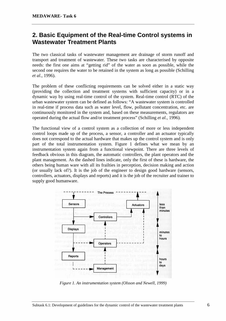
2. Basic Equipment of the Real-time Control systems in Wastewater Treatment Plants The two classical tasks of wastewater management are drainage of storm runoff and transport and treatment of wastewater. These two tasks are characterised by opposite needs: the first one aims at “getting rid” of the water as soon as possible, while the second one requires the water to be retained in the system as long as possible (Schilling et al., 1996). The problem of these conflicting requirements can be solved either in a static way (providing the collection and treatment systems with sufficient capacity) or in a dynamic way by using real-time control of the system. Real-time control (RTC) of the urban wastewater system can be defined as follows: “A wastewater system is controlled in real-time if process data such as water level, flow, pollutant concentration, etc. are continuously monitored in the system and, based on these measurements, regulators are operated during the actual flow and/or treatment process” (Schilling et al., 1996). The functional view of a control system as a collection of more or less independent control loops made up of the process, a sensor, a controller and an actuator typically does not correspond to the actual hardware that makes up the control system and is only part of the total instrumentation system. Figure 1 defines what we mean by an instrumentation system again from a functional viewpoint. There are three levels of feedback obvious in this diagram, the automatic controllers, the plant operators and the plant management. As the dashed lines indicate, only the first of these is hardware, the others being human ware with all its frailties in perception, decision making and action (or usually lack of?). It is the job of the engineer to design good hardware (sensors, controllers, actuators, displays and reports) and it is the job of the recruiter and trainer to supply good humanware.

Figure 1. An instrumentation system (Olsson and Newell, 1999)

MEDAWARE- Task 6


The displays and reports are often overlooked by the engineer. However they are very important in ensuring that the humanware gets the right message and hence have the best chance of making the right decision and enhancing rather than degrading the performance of the system as a whole. In selecting a hardware instrumentation system the important criteria typically include:

• Suitability. The equipment must of course do the job required.

• Availability. The instrumentation should not cause undue interruptions to production. The importance of this depends upon the process. It is a key issue for large continuous processing plants but less of an issue for small batch processing plants. This determines the chosen architecture and the degree of redundancy.

• Reliability. Even if the availability criterion is met we don't want frequent problems.

• Ease of use. This a key issue in achieving the best possible interface between the hardware and the humanware. What are the facilities for simple operator interaction, developing good displays and reporting systems, and interfacing to plant information systems?

• Ease of maintenance. Is the equipment accessible? Can faulty parts be replaced on-line? What sorts of diagnostics are available? What is the backup in parts and expertise from the manufacturer?

• Cost. Again this is the deciding factor all else being equal. Again it is a trade-off of cost against advantages in the above areas since usually things are not equal.

The control system interfaces with the plant through the actuators and sensors. There is no sense making sophisticated decisions if they are not implemented. It stands to reason that these two classes of instrumentation are the key to successful process control. Many "control problems" are caused by our poor selection of or our neglect of the basic sensors and actuators.

2.1 Sensors A sensor is an instrument that is capable of obtaining information directly from an object or process and that presents this information in such a way that one is able to deduce the variable to be measured. We may recognize some special features of an on-line sensor:

• The sensor should be located in the process. • The sensor output should be considered continuous with respect to the process

time scale. • The sensor should be operated without continuous human intervention.

Since the sensor environment is usually quite hostile in a wastewater treatment plant, it is even more essential to prove the reliability of the sensors and the usefulness of the data. There is still a great challenge to convince design engineers, environmental managers and operators to use some of the mentioned instruments.

MEDAWARE- Task 6


Several factors have to be considered in the selection of sensors. Here we will mention the most important ones: Selection and location of sensors. Selection: From the perspective of a control engineer the first design issue as far as sensors are concerned is the selection of the right one for the application from a bewildering range of possibilities. Factors to be considered are:

• Type of sensor. • Range. Choosing the desired sensor range can depend on the minimum and

maximum values encountered during operation, on the desired sensitivity to deviations caused by disturbances and on the desired accuracy of measurement. Additional sensors in parallel with different ranges are occasionally required.

• Linearity. If the sensor output signal varies linearly over the measurement range subsequent display and processing is greatly simplified. For a linear sensor the deviation from linear should be less than the accuracy.

• Accuracy. Is important that the output signal always give the same or much closed value for the same measurement value. Typical values are less than one per cent of range.

• Drift. How quickly does the calibration change? Re-calibration of instruments is costly so you would like to keep it to a minimum. Modern electronic sensors are quite good in this regard.

• Speed of response. Typically sensors will settle out in one or two seconds. This can be important where very fast acting control is necessary or for complex sensors which can respond much more slowly.

• Cost. Location of Sensors: The second design issue as far as sensors are concerned is where they should be located. There are several factors to be considered:

• Dead time.(sensitivity) The time between the changes in the process variable occurring and the time that changes reaches the sensor should be as short as possible.

• Environment. Most sensors are constructed for field mounting. That is they can be mounted basically anywhere. On-line composition analyzers on the other hand usually require a laboratory-type environment, for example in an air-conditioned or heated analyzer house.

• Sample condition. Many sensors require samples in a particular condition either to function at all or to give the specified accuracy. The flow pattern at an orifice plate must be well developed with straight lengths of pipe before and after the sensor. Analyzers where the sample must be vaporized or condensed first require elaborate processing to ensure no changes in composition or excessive dead time.

• Maintainability. For maintenance purposes the sensor should be easily accessible, beside a walkway rather than out of reach. Special piping or valving may be needed to allow removal without shutting down the process or to enable in situ recalibration.

MEDAWARE- Task 6


Location should be specified on piping and instrumentation diagrams, preferably explicitly by notes if there is any ambiguity possible.

The sensors in a common WWTP can be used in many ways:

• Monitoring: Where the sounding makes continuous follow of the main variables of the process.

• Feedback Control: This type of control makes a fallow of several variables and makes an action over the variable to retrieve the set-point of the process. This uses direct measurements of the controlled variables.

• Anticipated (Feed forward) Control: in this type of control the perturbation is measured, and the control action is made to minimize the effect of the perturbation in the process.

• Distributed Control: This kind of control can keep the plant running by a large number of local controllers for physical variables. The distributed control systems by PLC’s, usually implemented as a Supervisory Control and Data Acquisition (SCADA) systems provides a robust control over the process faults and enables system supervisory.

Examples of the typical sensors in WWTP are in Table 1:

Table 1: Level of instrumentation at WWTPs. (Jeppsson et al., 2001)

Parameter Usage Used for Temperature +++ M Conductivity ++ M PH +++ M Redox Potential ++ M Air Pressure ++ M Water Level ++ M Water Flow +++ M,B,F Air Flow +++ M,B Dissolved Oxygen (DO) +++ M,B Turbidity +++ M Total Suspended Solids ++ M Sludge Blanket Level + M BOD5 + M COD + M TOC + M Ammonia + M Nitrate + M Total Nitrogen + Phosphate + M Total Phosphorus + M Respiration, activity + M Toxicity + M Sludge Volume Index +

The main purpose of the measurements: + seldom used; ++frecuently used; +++ normally

used; M:Monitoring; B:Feedback Control; F:Feed forward Control Next we discuss the different sensor typically used in WWTP

MEDAWARE- Task 6


First we will identify a number of physical sensors for gas and liquids flow rate, level, pressure and temperature.

• Flowrate:

Flow rate measurement is fundamental in any wastewater treatment process. Measuring flow rate is far from trivial and it is difficult to do it with great accuracy. There are different principles or mechanism for volumetric flow rate measurements: Table 2: Typical sensors for flowrate

Type Mechanism Applications Orifice plate Pressure drop over orifice

type restriction Clean liquids and gases; nonlinerar; low range

Vortex Frecuency of vortices in wake of bluff body

Clean liquids and gases; linear; better range

Electromagnetic Emf induced in magnetic field

Slurries, dirty liquids, food; fluid must be conductive; expensive

Turbine Speed of rotation of turbine or propeller

Clean liquids and gases; very good repeatability and rangeability

Ultrasonic Transmitting and receiving ultrasonic pulses

Both the magnetic flow meter and the meters based on ultrasonic techniques have the advantage that they are non invasive meters and have less need for servicing than other contact-flow devices

• Level:

The common sensors found in WWTP for level are:

Table 3: Typical sensors for level (Olsson and Newell,1999)

Type Mechanism Applications Displacement Weigh change due to liquid

displacement Clean liquids; levels or interfaces; installed in standpipe

Differential Pressure

Hydrostatic head or liquids between taps

Liquids; seals if dirty or corrosive

Capacitance Changing dielectric constant between material and air

Liquids or granular solids; insulate if material conductive

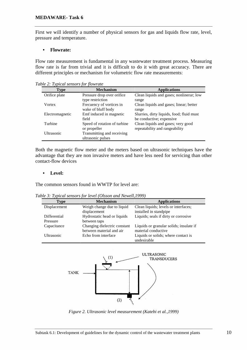
Ultrasonic Echo from interface Liquids or solids; where contact is undesirable

Figure 2. Ultrasonic level measurement (Katebi et al.,1999)

MEDAWARE- Task 6


Figure 2 shows an application of ultrasound techniques to level measurement. In one situation (1) the meter is placed above the tank and the time take for the pulse to be reflected from the surface of the fluid is measured. In the second example (2) the transducer is place below the tank and the time taken for the echo to reach the surface of the liquid and return is measured.

• Pressure:

The common sensors found in WWTP for pressure are: Table 4: Typical sensors for Pressure

Type Mechanism Applications Bourdon tube Motion or torque at closed

end of curved or spiral tube Gauges; gases or clean liquids; seals if dirty or corrosive

Diaphragm Force or displacement by capacitance, piezolelectric, strain gauges

Sensors; gases or clean liquids; seals if dirty or corrosive

• Temperature:

The common sensors found in WWTP for temperature are:

Table 5: Typical sensors for Temperature (Olsson and Newell,1999) Type Mechanism Applications

Thermocouple Emf generated at junction of dissimilar metals

Type T (-200ºC to 350ºC) Type J (-200ºC to 750ºC) must be dry Type K (-200ºC to 1100ºC) oxidising sulphur-free environment Type S/R (0ºC to 1450ºC) oxidising environment

Resistance (RTD) Change in resistance of metals with temperature, typically platinum

Typically -260ºC to 800ºC

Pyrometers Measures thermal radiation intensity focused optically

0ºC to 4000ºC; requires clear line of sight

Another fundamental measurements for wastewater treatment operations are physical or chemical properties of the wastewater such as turbidity, solids content, settleability, conductivity and oxidation-reduction potential (ORP or redox potential)

• Turbidity: Insoluble particles of soil, organics, microorganisms and other material impede the passage of light through water by scattering and absorbing the rays. This interference of light passage through water is referred as tubidity. Turbidity (thickness) and suspended solids are often measured by using either the principles of light absorption or the principle of light scattering.

MEDAWARE- Task 6


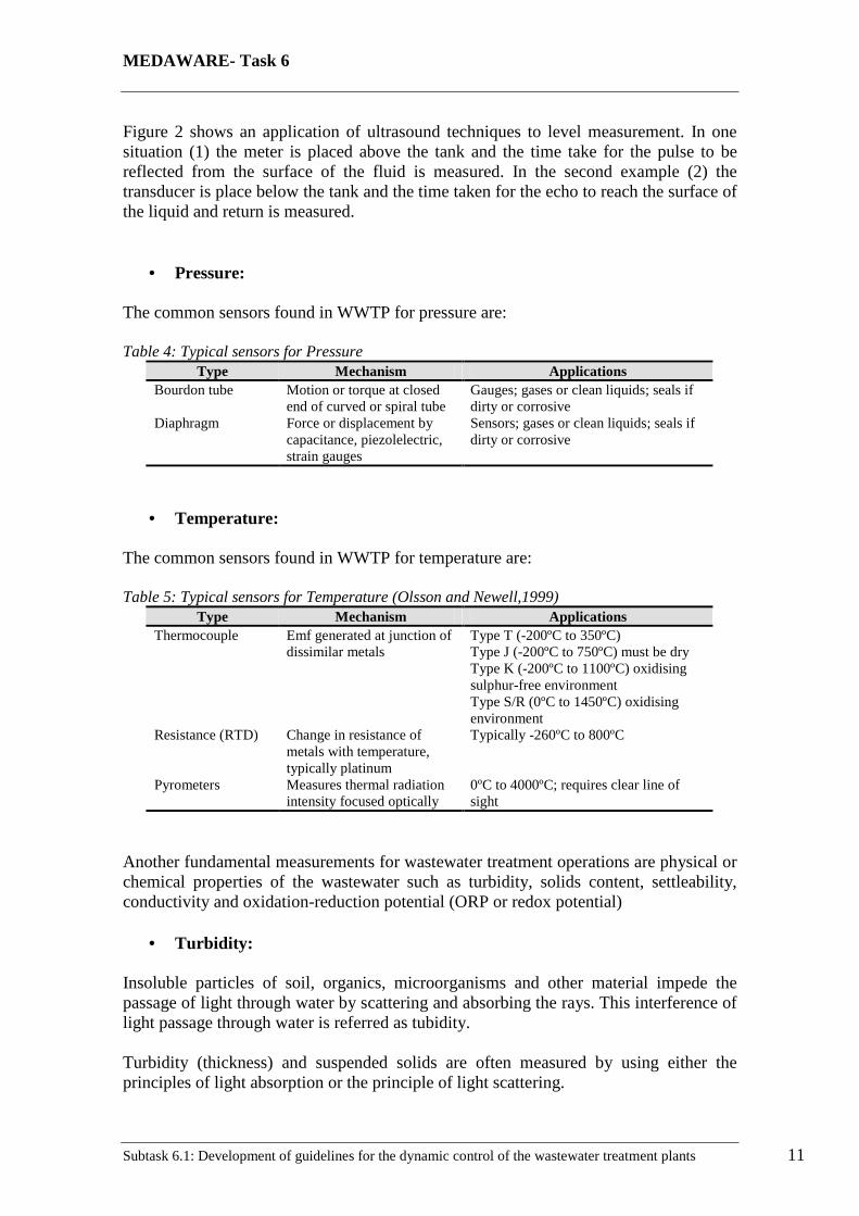
An example of an absorption sensor is shown in Figure 3. The sensor is immersed to the required depth in a tank. The light source (LED) is regulated by the sensor system and emits light through an optical sensing gap to a photocell, which senses the amount of light transmitted through the liquid. This will produce an electrical signal related to the turbidity or the suspended solids concentration of the liquid.

Figure 3. Turbidity sensor using light absorption techniques. (Katebi et al.,1999)

• Solids content:

Monitoring suspended solids is important to ensure compliance with local authority requirements, to gain early warning of plant failure, and to asses the effectiveness of the WWTP. Total suspended solids can be determined on-line using scattered light or light absorbance.

• Settleability: Currently there is a striking lack of sensors or analysers that can meet the need for settling information. The traditional way of quantifying sludge settleability is by measuring the sludge volume index (SVI). Various approaches to designing on-line settlometers have been reported. The overall operation of a wastewater treatment plant depends crucially on the settling properties so a reliable and frequent measurement of sludge settling is highly motivated. One approach is to install a measuring system that tracks the sludge blanket of concentration profiles in the full scale clarifier, while another methodology consists of using a down-scaled version of the device under study in a measuring systems and performing experiments in this model reactor. The last approach is based in Image processing using High resolution microscopes.

• Conductivity:

Conductivity is a measure of the ability of a solution to carry an electric current. This ability is dependent on the presence of ions, their total concentration, mobility, valence, relative concentrations and the temperature.

MEDAWARE- Task 6


Conductivity can be a qualitative measure and rapid determination of large changes in inorganic content of water and wastewater. Conductivity sensors can give continuous measurements of conductivity if they are properly installed and maintained.

• Redox potential:

The oxidation-reduction potential (ORP), often called the redox potential, is an indication of the oxidation state of a specific monitored systems. The redox potential often displays a “knee” or breakpoint in anoxic operation. Thus the redox provides information of biological processes in particular during anoxic and anaerobic conditions. Since the measurement is relatively unproblematic and quite accurate there is an obvious incentive to use the redox potential for control purpose. Next, we will describe some important measuring principles for the analysis of wastewater composition. Most of the chemical and biologic sensors should be used in-line with automatic sample conditioning. Pre-treatment of the samples is most often required to ensure satisfactory operation of the sensors equipment. Sensors requiring pre-treatment include nutrient analysers: ammonium, nitrate and phosphate analysers. The sampling unit is meant to remove threads and suspended solids that would otherwise block tubes, pumps and measuring cells or result in fouling of the electrode.

• Dissolved Oxygen Measurement:

Dissolved Oxygen determination is a key measurement in wastewater treatment. For example the DO concentration is the basis for the determination of respiration rates. It is crucial to keep the DO sufficiently high in aerators and sufficiently low in anoxic reactors. For on-line measurements the DO is measured without a chemical treatment of a sample. A DO probe is composed of two solids metal electrodes in contact with a salt solution that is separated from the water sample by a selective membrane. The probe also has a sensor for measuring temperature. The unit can be submerged in an aeration tank for DO and temperature measurements. The membrane electrodes may be calibrated by reading against air as well as a water sample of known DO concentration determined by the iodometric method.

Membrane electrodes have been used for DO measurements in lakes and reservoirs, for control of industrial effluents and for continuous molecular measuring of the DO in activated sludge systems.

• Acid or Base Character:

Measurement of pH is one of the most important and frequently used test in water chemistry. Practically every phase of water supply and wastewater treatment such as

MEDAWARE- Task 6


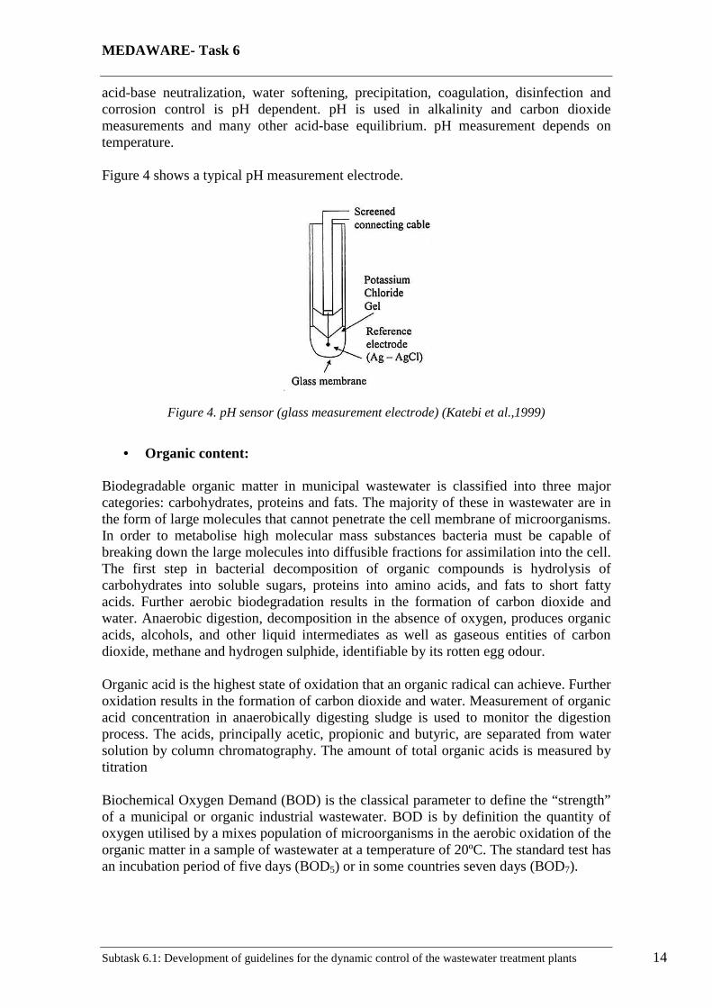
acid-base neutralization, water softening, precipitation, coagulation, disinfection and corrosion control is pH dependent. pH is used in alkalinity and carbon dioxide measurements and many other acid-base equilibrium. pH measurement depends on temperature. Figure 4 shows a typical pH measurement electrode.

Figure 4. pH sensor (glass measurement electrode) (Katebi et al.,1999)

• Organic content:

Biodegradable organic matter in municipal wastewater is classified into three major categories: carbohydrates, proteins and fats. The majority of these in wastewater are in the form of large molecules that cannot penetrate the cell membrane of microorganisms. In order to metabolise high molecular mass substances bacteria must be capable of breaking down the large molecules into diffusible fractions for assimilation into the cell. The first step in bacterial decomposition of organic compounds is hydrolysis of carbohydrates into soluble sugars, proteins into amino acids, and fats to short fatty acids. Further aerobic biodegradation results in the formation of carbon dioxide and water. Anaerobic digestion, decomposition in the absence of oxygen, produces organic acids, alcohols, and other liquid intermediates as well as gaseous entities of carbon dioxide, methane and hydrogen sulphide, identifiable by its rotten egg odour. Organic acid is the highest state of oxidation that an organic radical can achieve. Further oxidation results in the formation of carbon dioxide and water. Measurement of organic acid concentration in anaerobically digesting sludge is used to monitor the digestion process. The acids, principally acetic, propionic and butyric, are separated from water solution by column chromatography. The amount of total organic acids is measured by titration Biochemical Oxygen Demand (BOD) is the classical parameter to define the “strength” of a municipal or organic industrial wastewater. BOD is by definition the quantity of oxygen utilised by a mixes population of microorganisms in the aerobic oxidation of the organic matter in a sample of wastewater at a temperature of 20ºC. The standard test has an incubation period of five days (BOD5) or in some countries seven days (BOD7).

MEDAWARE- Task 6


The BOD test is not a precise measurement and the reproducibility is quite poor. Test on real wastewaters normally show standard deviation of 10-20 per cent. Chemical Oxygen Demand (COD) is widely used to characterise the organic strength of wastewaters. The test measures the amount of oxygen required for chemical oxidation of organic matter in the sample to carbon dioxide and water. There is no uniform relationship between COD and BOD of wastewater except that the COD value must be greater than the BOD. The correlation for a particular wastewater can be determined. Total Organic Carbon (TOC) measures the organically bound carbon in a water or wastewater sample. Unlike BOD or COD it is independent of the oxidation state of the organic matter but does not provide the same kind of information. TOC does not measure other organically bound elements such as nitrogen, hydrogen and inorganic that can contribute to the oxygen demand measured by BOD and COD. Therefore TOC does not replace BOD or COD.

• Nutrient Analysers: Since the purpose of nutrient removal plants is to remove nitrogen and phosphorus, there is an obvious interest in measuring these substances. The focus has to been placed on sensors for ammonium (NH4), nitrate (NO3) and phosphate (PO4). The measurement of total N and P is interesting for influent and effluent monitoring purposes but to the date there are only a few manufactures of such sensors and the instruments are very expensive. There are two main principles for ammonium sensors, the gas electrode sensors and a colorimetric sensor. Determination of nitrate is difficult because the relatively complex procedures required. For nitrate there are three main principles used in common sensors:

- Electrode sensors: the response time is less than 10 minutes - Sensors using direct photometry: This is based on ultraviolet(UV)

absorption and no reagents are used. The response time is less than 5 minutes.

- Sensors based on colorimetry. Nitrite is an intermediate oxidation state of nitrogen both in oxidation of ammonia to nitrate and in the reduction of nitrate. Nitrate can be determined by photometric measurements in the range 5 to 50 µg N/l if a 5 cm light path and a green colour filter are used. Higher concentrations can be determined by diluting a sample. Phosphorus occurs in natural waters and wastewaters almost solely as phosphates. Phosphates also occur in bottom sediments and in biological sludges both as precipitated inorganic forms and incorporated into organic compounds. Phosphate sensors are generally more complex than the ammonia or nitrate sensors since the reactions taking place are more complex. Some coloured substance is formed

MEDAWARE- Task 6


from the phosphate and the colour development is quantitatively measured using a spectrophotometer. There are two major colorimetric methods used: the vanadomolybphosphoric acid method and the molybdenum blue method. Commercial phosphate analysers are based on the photometric principle and both the principles above are implemented.

• Optical sensing: A considerable amount of research has been devoted to the development or rapid techniques to replace the traditional BOD, COD, and TOC measurements for organic content. Absorption at particular wavelengths has been found to correlate well with BOD, COD and TOC values. This research has led to commercial products, however the extensive use of such instrumentation has been severely frustrated by sensor fouling. This instrumentation usually requires pre-sample filtration and frequent washing leading to increased maintenance. To overcome these difficulties there has been a shift towards the development of biosensors and flow injection.

• Respirometry: Respirometry is the measurement and interpretation of the respiration rate of activated sludge. The respiration rate is the amount of oxygen consumed by the micro organisms measured per unit volume and unit time. The respiration rate reflects two of the most important biochemical processes in a WWTP, biomass growth and substrate consumption. Respirometry has been the subject of many studies and a number of measurement techniques and instruments have been developed. Sometimes the term BOD monitor is used for respirometers. This is not to be confused with BOD5 since the measures oxygen consumption using a biomass adapted to the wastewater typically during a few minutes. The IWAQ task group has pointed out that there are only eight basic principles of respirometers according to these basic principles:

- measurement in liquid or in gas phase - flow regime of liquid (flowing or static) - flow regime of gas (flowing or static)

Before, the weakest part of the control chain were the sensors that caused problems in calibration, fouling, reliability and sampling techniques Today, the performance and reliability of many on-line sensors (e.g. nutrient sensors, respirometers) have improved remarkably during the last decade (if maintained properly). The most fundamental barrier for more widespread acceptance of new control strategies is that existing WWTPs are not designed for RTC.

MEDAWARE- Task 6


2.2 Actuators The predominant actuator in process plants remains the control valve, for adjusting the flow rate of gases, liquids, slurries and solids. Variable-speed drives (electric or hydraulic motors) are often used for solids conveyors and increasingly for pumps and compressors where they are displacing control valves. The cost of a variable-speed drive remains high but if the pressure loss across the control valve is expensive then it can be more economical in the longer term. With these actuators we operate the WWTP. Table 5 and Figure 5 show the variables commonly used to operate WWTPs.

Table 5. WWTP variables avaliable for manipulation.

Manipulated variable Process Applicability Bypass/Overflow 1,2 ∀ Equalisation/Buffeting/Storm tanks 1,2 ∃ Feeding point/Step point 1,2 ∃ Aeration intensity 1,2 ∀ External Carbon Source 2 ∀ Internal Recycle Flow rates 2 ∃ Chemical dosage 2,3 ∃ Return Activated Sludge rate A ∀ Waste Activated Sludge rate A ∀ Sludge storage ∀ ∃

Process: 1-activated sludge; 2-nutrient removal; 3-sedimentation; A-all

Applicability: ∀-state of technology; ∃-applicable in certain cases.

Figure 5. Overview of control handles in an activated sludge WWTP.

MEDAWARE- Task 6


2.2.1 Pump and Compressor Drive Systems Using a motor there are three main ways to control a flow or to transfer liquid, slurry, air, gas or other objects during a given period. The main methods are based on:

• constant speed motor, • combinations of two or more sets of equipment providing step-by-step control

of the drive, and • variable speed motor.

Each main group can then be sub-divided into sub-groups according to the design and function of the drive system. For example a variable speed motor drive can be divided into three sub-groups:

• mechanical control, • hydraulic control, and • power electronic control.

Constant Speed: The simplest way to control a motor is to use on/off switches. By shutting off the motor when it is not needed unnecessary use of energy is eliminated in the same way as with a light switch. This is still quite common in treatment plants like for influent flow rates. From an equipment point of view there is a serious drawback due to the mechanical wear which is apparent when large flow rates and pressures are controlled. Frequent starts and stops can radically limit the life of the equipment due to the pressure surges. From a process point of view on/off control is mostly negative. We can see that sudden flow rate changes will have a significant influence on the clarifier behavior. Also wide swings of the dissolved oxygen control will deteriorate the biological behavior Throttling is an old method of flow control and uses a damper or a throttle valve to restrict the flow for example in the piping. Independent of the valve position the pump operates continually at full speed .Guide vane control is a common way to control the air volume from a fan. The technique is used over a wide flow range. Compared to these control methods variable pitch control represents a more advanced type of control for both fans and pumps. efficiency over a wide flow range. Step-by-Step Control: To utilize energy more efficiently and to achieve a better pressure and flow capacity, fans as well as pumps can be connected in series or in parallel. It is then possible to use a constant-speed pump for base flow and a variable speed pump to cover the variable speed range. It is also possible to have two pumps that operate alternately with one running continuously in the daytime and the other in the night-time. The pumps then alternate as duty and standby pumps. Twin pumps are often used providing a stand-by and an option for different capacities. Variable Speed Control: There are several ways to introduce variable speed control. The torque can be transferred between the motor and the load axes without any mechanical contact. In a hydraulic coupling the required speed is achieved through an oil slip between blades mounted on the motor shaft and the pump shaft in a rotating oil

MEDAWARE- Task 6


container. The speed on the pump shaft is varied by changing the oil level in the container. The motor runs at constant speed. Eddy current couplings have been used for many decades to synchronize speeds between a constant-speed electric motor and a load, but the most elegant and potentially the most versatile control method is by power electronic control using a frequency converter. Frequency converters have been developed since the 1960s and are today a mature and well proven technology. The development of power electronic circuits and control electronics has made frequency control affordable and reliable. When considering variable speed drives we mostly consider asynchronous (induction) motors since they are the dominating motor type in pump and compressor systems. Today there are frequency converters available for a very wide range of power from less than one kW to several thousand kilowatts. A particularly used method for control is pulse width modulation (PWM). A frequency converter can be used in both a new installation and in an old system. Since most pump or compressor systems already have an asynchronous (induction) motor they are in a sense prepared for frequency converter operation. In an advanced motor operation where a large operating range is going to be used the cooling of a standard motor may be insufficient at low speed and high torque. Then the motor may have to be supplied with extra cooling.

2.2.1 Control Valves A control valve consists of a shaped plug which is mounted on a stem and which moves up and down within a usually circular seat. The stem is usually moved by air pressure on a diaphragm opposed by a spring. The spring either opens or closes the valve depending on its desired state in the event of air supply failure. Occasionally an electric or hydraulic actuator is used to move the stem. The plug and seat and the valve body design varies to accommodate the pressure drop across them, the type of fluid and the desired shape of the flow rate vs. stem position characteristic. The valve body sizing is normally chosen to match the pipe size where the valve is located. The selection of valve body type and the sizing of the plug and seat combination requires consideration of the following factors:

• Pressure drop. Large pressure drops across control valves can make it difficult to move the valve stem. Special body designs divide the flow into opposite directions through two plug-seat combinations to cancel out the forces. Small pressure drops require different types of valves such as butterfly valves.

• Maximum flow rate. This should be the maximum design flow rate plus the maximum control action. Ideally the latter should be 30-50 % of the design flowrate although many non-control engineers hamstring control loops by cutting this margin to as little as 10 % (and then complain about the performance). The valve size is specified by the Cv,max parameter calculated from the flowrate and pressure drop.

MEDAWARE- Task 6


• Rangeability. This is the ratio of the flow rates for stem positions of typically 15 and 85 % (100 % is full open). It is related primarily to the plug and seat design and the pressure drop vs. flow rate characteristic which is often related to the pump upstream of the valve. Again the rangeability must account for the normal range of operating flow rates with an adequate control margin (preferably 30 to 50 %) both below and above that range. Different sized valves in parallel are occasionally required.

• Sensitivity. This relates to the rangeability and the amount of control action required to control to the desired accuracy. Occasionally a large valve is required to set the nominal flow rate and a small valve in parallel is used to achieve the desired sensitivity.

• Linearity. For a control loop the objective is that the sensor output vs. controller output relation for the valve plus process plus sensor is linear. This means that often the valve characteristic and occasionally the sensor characteristic is chosen to compensate for nonlinearities of the process or sensor. If this linearity is not achieved poor control loop performance is likely without special controllers.

• Hysteresis. This is a common problem with control valves due to seal friction where the stem enters the body of the valve due to the fluid pressure drop across the valve. It is a common cause of small continuous oscillations in control loops. A valve positioner is the recommended solution. It is a special high-gain secondary control loop which measures stem position and applies strong control action to achieve the desired stem position requested by the primary controller.

MEDAWARE- Task 6


2.3 Controllers and Control Systems The design and provision of control systems with the capabilities to integrate a large number of plant functions have been a major concern for control practitioners since the Sixties. The early attempts to produce a working integrated system were concentrated on the application of a central digital computer to plant wide control. This was achieved by the replacement of pneumatic and analogue equipment such as sensors and actuators with their digital or high power electronic counterparts. They are in approximate historical order with single loop controllers ruling from before World War II until the sixties, distributed control systems (DCS) from the seventies to the present, programmable logic controllers (PLC) from the eighties to the present, and PC or workstation systems from the nineties. The discussion will omit the systems based on mini to mainframe computers, the so-called direct digital control (DDC) systems, which were developed in the sixties and are now largely extinct.

2.3.1 Single Loop Controllers Sensors and actuators are nearly always separate pieces of hardware (some ex- ceptions in the case of sensors will be discussed later). Controllers can also be completely separate hardware each with its own displays and adjustments for individual loops. They are in old process plants, very small systems (on local control panels) or critical high-availability systems. They are the ultimate from the high availability viewpoint as only one loop at a time is likely to be affected by a hardware failure, assuming separate and secure power supplies. The problem is that the display and adjustment functions as well as the control function are fully distributed. This resulted in the often very large control panels which made the interface with the operator difficult. It also required more operators with the inherent communication and coordination problems.

2.3.2 Distributed Control Systems The development of the microprocessor led to the rise of the distributed control system or DCS for short. Despite its name the DCS is a compromise between single loop controllers and the now extinct direct digital control (DDC) system. The latter implemented large numbers of control loops on a single computer which centralised the display and reporting function. However they were an availability nightmare especially since computers in the seventies and eighties were not nearly as reliable as they are now. The DCS basically implements the control loops in small groups, each group having its own microprocessor which is often duplicated. The microprocessors are then connected via a data highway to which one or more centralised display stations are connected. The data highway is also frequently duplicated.

This arrangement gives us the best of both worlds. We can have the control functions as separated as we like (a cost vs. availability trade-off) and the display, adjustment and reporting functions centralised for ease of operation. The DCS is most suited to medium

MEDAWARE- Task 6


(tens of loops) to large (hundreds of loops) continuous processing plants although more recent systems can also be applied to large batch processing plants. The major problem with the DCS is that there are several major manufacturers (such as Honeywell, Bailey, Yokogawa, Foxboro, ABB, Siemens) in a very competitive market with essentially proprietary systems. These systems will not interconnect and in many cases connect with general purpose computer (information) systems only at considerable expense. The latter problem is at least being addressed in more recent systems but interconnection at the operator level remains virtually impossible.

2.3.3 Programmable Logic Controllers (PLC) Before the advent of the microprocessor sequences of operations (batch plants and equipment startup and shutdown) were implemented with complex systems of relays. These were expensive to build and maintain and changes were a major exercise. The programmable logic controller (PLC) was developed to address this need and has now virtually eliminated relay systems in processing and manufacturing plants. The PLC consists of a microprocessor, digital inputs for detecting switch positions, digital outputs for activating solenoids or switches, and a simple interface for programming the sequences into the microprocessor. Early interfaces used the ladder logic terminology (intelligible only to instrument personnel) but more recent interfaces use another high level languages or even higher level representations (GRAFCET).

Actually PLCs have also incorporated analog signal interfaces and even the capability to implement feedback and feedforward control loops. One or more of these can be interfaced to a personal computer as an operator console, These PLCs are often used for batch processing plants and small (low tens of loops) continuous processing plants.

2.3.4 Personal Computer and Workstation Systems More recently a large number of control packages have become available on per-sonal computers (PCs) and UNIX workstations. The connection to plant signals is implemented by interface cards which plug into the computer, by interface cards which plug into separate boxes connected to the computer, or by a PLC connected to the computer. In some cases a dedicated microprocessor or a PLC is used to implement some or all of the control functions leaving the PC for display and higher level control functions. These systems are used for small batch or continuous processing applications (low tens of loops). They can suffer from reliability problems particularly those which utilise personal computers and operating systems not designed for real-time applications (DOS and Windows for example). The response time in a WWT plant application should not be a problem and an operating system like Windows NT is considered sufficiently fast. Using the techniques of 1999 a typical response time for a PC for real-time control is about 3-500 ms. Since the operating system works with interrupts it also gives a lot of flexibility. Each real-time program can be processed in its own time scale so the real-time demands would not be crucial for a process control application like WWT. On the

MEDAWARE- Task 6


other hand the reliability is still not up to the requirements in many applications. Who has heard of viruses in PLCs? Unfortunately they are a reality in PCs. However PCs are a relatively low-cost solution at least in the short term.

Recently there has been an obvious development where PLCs are completely replaced by personal computers. The development has been called "soft PLCs".There are also many objections to the "soft PLC" solution. Since the PC is a standard product it may be much less efficient for some control tasks. Probably open systems like PCs will probably create difficulties when components of different brands are to be connected. On the other hand the economy is a strong driving force. The 1996 market for personal computers is about USD 100 billion and for PLCs only about USD 4 billion. This opens up a huge market for general control software. There are already some control packages available on the market.

Usually the real limitation in a PC based computer control system is the bus capacity. In order to connect the computer to the physical processes you can use an interface card to which each signal has to be connected or you can use some bus to connect the signals. Then there is a remote processor close to the sensor where the primary signal processing takes place. Such fieldbus structures are further discussed.

MEDAWARE- Task 6


3. Control The purpose of most wastewater automatic control system is to maintain one or several process parameters as SRT, DO, or clarifier signal depth at a fixed value. If there were no changes in external conditions, such as flowrate variation, process control would be a simple task. However, external conditions are changing constantly, and, as a result, some dynamic control over treatment processes is needed. Therefore, Control is necessary to operate the WWT Plant towards a defined goal, despite different factors that cause a change in the operation of performance of a treatment process (disturbances). The main aims of the control options in WWTP can be summarised as follows (Schütze et al., 2002):

• Avoidance of discharge of biomass into effluent. • Maintenance of performance of the plant processes. • Maintenance of the overflow discharge and effluents standards. • Minimization of operation and maintenance costs.

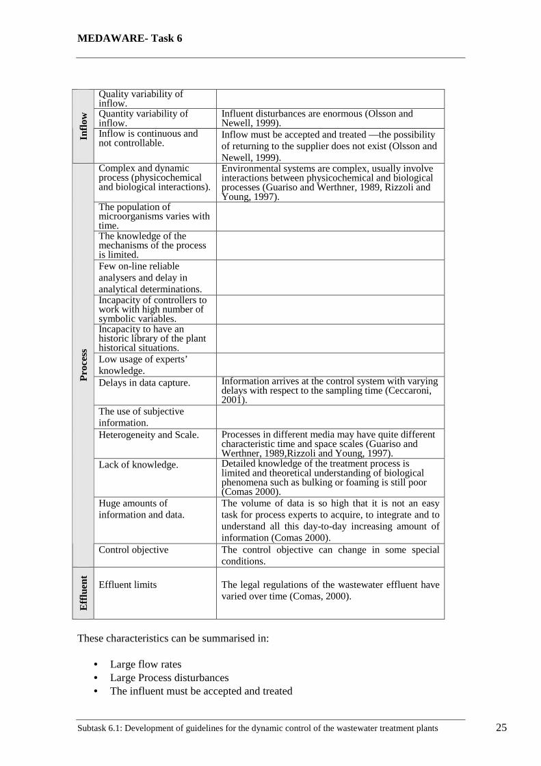
The typical characteristic of a WWT plant are: Table 6. Environmental systems and WWTP characteristics (Cortes, 2002)

Dynamic. Environmental systems evolve over time (Guariso and Werthner, 1989, Rizzoli and Young, 1997). They are subject to continuous changes that can directly modify the performance of the process (Miquel Sànchez et al. ,1996).

Spatial coverage. Environmental systems involve physical processes which take place in a 2- or 3- dimensional space (Guariso and Werthner, 1989, Rizzoli and Young, 1997)

Randomness. Many environmental processes are stochastic. In addition, the parameters of models representing such processes are usually uncertain, and their ranges are commonly known only approximately. These attributes call for techniques such as statistical analysis and qualitative analysis of model equations (Guariso and Werthner, 1989, Rizzoli and Young, 1997)

Periodicity. Many environmental processes are periodic in time, which adds a degree of complexity to parameter calibration and validation (Guariso and Werthner, 1989, Rizzoli and Young, 1997).

Reliability: Important maintenance efforts are necessary for the reliable functioning of the on-line analysers (for ammonia, nitrite, nitrate and dissolved oxygen) on which the data models are based (Ceccaroni, 2001).

Non-linearity The reactions of the activated sludge process often reach pseudo stability when substrates, nutrients or oxygen are limited (Comas, 2000).

Gen

eral

Cha

ract

eris

tics

The WWTP domain ill-structure

Enviromental systems are poor-or-ill-structured domains (Comas 2000). Mathematical models often are unable to represent biological processes because these do not follow an established pattern.

MEDAWARE- Task 6


Quality variability of inflow.

Quantity variability of inflow.

Influent disturbances are enormous (Olsson and Newell, 1999).

Inflo

w

Inflow is continuous and not controllable.

Inflow must be accepted and treated —the possibility of returning to the supplier does not exist (Olsson and Newell, 1999).

Complex and dynamic process (physicochemical and biological interactions).

Environmental systems are complex, usually involve interactions between physicochemical and biological processes (Guariso and Werthner, 1989, Rizzoli and Young, 1997).

The population of microorganisms varies with time.

The knowledge of the mechanisms of the process is limited.

Few on-line reliable analysers and delay in analytical determinations.

Incapacity of controllers to work with high number of symbolic variables.

Incapacity to have an historic library of the plant historical situations.

Low usage of experts’ knowledge.

Delays in data capture. Information arrives at the control system with varying delays with respect to the sampling time (Ceccaroni, 2001).

The use of subjective information.

Heterogeneity and Scale. Processes in different media may have quite different characteristic time and space scales (Guariso and Werthner, 1989,Rizzoli and Young, 1997).

Lack of knowledge. Detailed knowledge of the treatment process is limited and theoretical understanding of biological phenomena such as bulking or foaming is still poor (Comas 2000).

Huge amounts of information and data.

The volume of data is so high that it is not an easy task for process experts to acquire, to integrate and to understand all this day-to-day increasing amount of information (Comas 2000).

Pro

cess

Control objective The control objective can change in some special conditions.

Effl

uent

Effluent limits

The legal regulations of the wastewater effluent have varied over time (Comas, 2000).

These characteristics can be summarised in:

• Large flow rates • Large Process disturbances • The influent must be accepted and treated

MEDAWARE- Task 6


• Concentrations are small • Process depends on micro-organisms • The product has to be consistently good

The main constraints are:

• Legislation • Education and training • Economy • Measuring devices • Plant constraint • Software

And the Incentives are:

• Effluent quality standards • Economy • Plant complexity • Improved tools

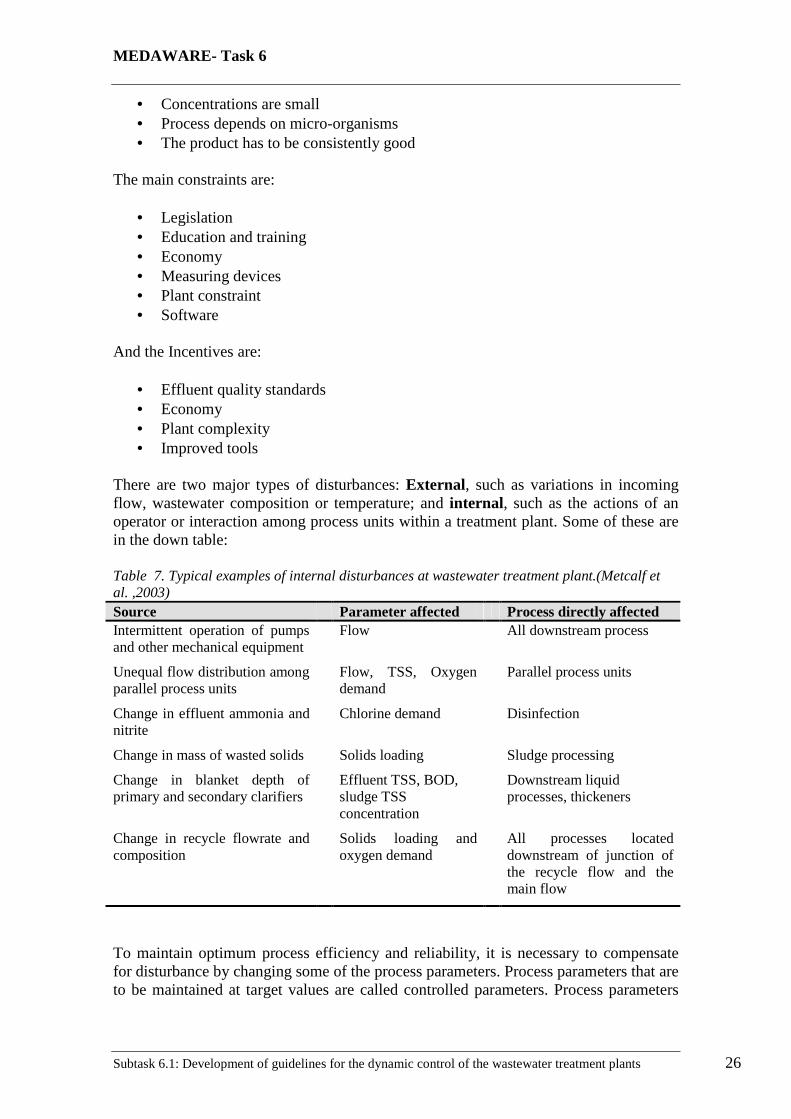
There are two major types of disturbances: External, such as variations in incoming flow, wastewater composition or temperature; and internal , such as the actions of an operator or interaction among process units within a treatment plant. Some of these are in the down table: Table 7. Typical examples of internal disturbances at wastewater treatment plant.(Metcalf et al. ,2003) Source Parameter affected Process directly affected Intermittent operation of pumps and other mechanical equipment

Flow All downstream process

Unequal flow distribution among parallel process units

Flow, TSS, Oxygen demand

Parallel process units

Change in effluent ammonia and nitrite

Chlorine demand Disinfection

Change in mass of wasted solids Solids loading Sludge processing

Change in blanket depth of primary and secondary clarifiers

Effluent TSS, BOD, sludge TSS concentration

Downstream liquid processes, thickeners

Change in recycle flowrate and composition

Solids loading and oxygen demand

All processes located downstream of junction of the recycle flow and the main flow

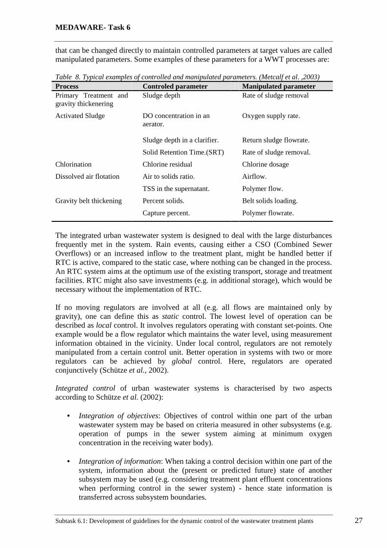
To maintain optimum process efficiency and reliability, it is necessary to compensate for disturbance by changing some of the process parameters. Process parameters that are to be maintained at target values are called controlled parameters. Process parameters

MEDAWARE- Task 6


that can be changed directly to maintain controlled parameters at target values are called manipulated parameters. Some examples of these parameters for a WWT processes are: Table 8. Typical examples of controlled and manipulated parameters. (Metcalf et al. ,2003) Process Controled parameter Manipulated parameter Primary Treatment and gravity thickenering

Sludge depth Rate of sludge removal

Activated Sludge DO concentration in an aerator.

Oxygen supply rate.

Sludge depth in a clarifier. Return sludge flowrate.

Solid Retention Time.(SRT) Rate of sludge removal.

Chlorination Chlorine residual Chlorine dosage

Dissolved air flotation Air to solids ratio. Airflow.

TSS in the supernatant. Polymer flow.

Gravity belt thickening Percent solids. Belt solids loading.

Capture percent. Polymer flowrate.

The integrated urban wastewater system is designed to deal with the large disturbances frequently met in the system. Rain events, causing either a CSO (Combined Sewer Overflows) or an increased inflow to the treatment plant, might be handled better if RTC is active, compared to the static case, where nothing can be changed in the process. An RTC system aims at the optimum use of the existing transport, storage and treatment facilities. RTC might also save investments (e.g. in additional storage), which would be necessary without the implementation of RTC. If no moving regulators are involved at all (e.g. all flows are maintained only by gravity), one can define this as static control. The lowest level of operation can be described as local control. It involves regulators operating with constant set-points. One example would be a flow regulator which maintains the water level, using measurement information obtained in the vicinity. Under local control, regulators are not remotely manipulated from a certain control unit. Better operation in systems with two or more regulators can be achieved by global control. Here, regulators are operated conjunctively (Schütze et al., 2002). Integrated control of urban wastewater systems is characterised by two aspects according to Schütze et al. (2002):

• Integration of objectives: Objectives of control within one part of the urban wastewater system may be based on criteria measured in other subsystems (e.g. operation of pumps in the sewer system aiming at minimum oxygen concentration in the receiving water body).

• Integration of information: When taking a control decision within one part of the

system, information about the (present or predicted future) state of another subsystem may be used (e.g. considering treatment plant effluent concentrations when performing control in the sewer system) - hence state information is transferred across subsystem boundaries.

MEDAWARE- Task 6


The control typical structure of a control system is termed a control loop. Control-loop systems are used to control flow, pressure, liquid levels, constituent concentrations, temperature, and other operating variables. The general control-loop structure exists in any type of control, whether manual or automatic Based on the performance records or numerous WWT Plants, automatic control systems not only reduce work-load, they also allow for more precise control of process parameters. Improved control of processes located downstream. Failure of any element (an instrument, most often) of an automatic control system may lead to serious problems if a control algorithm does not automatically recognize such a failure has occurred and compensate for it.

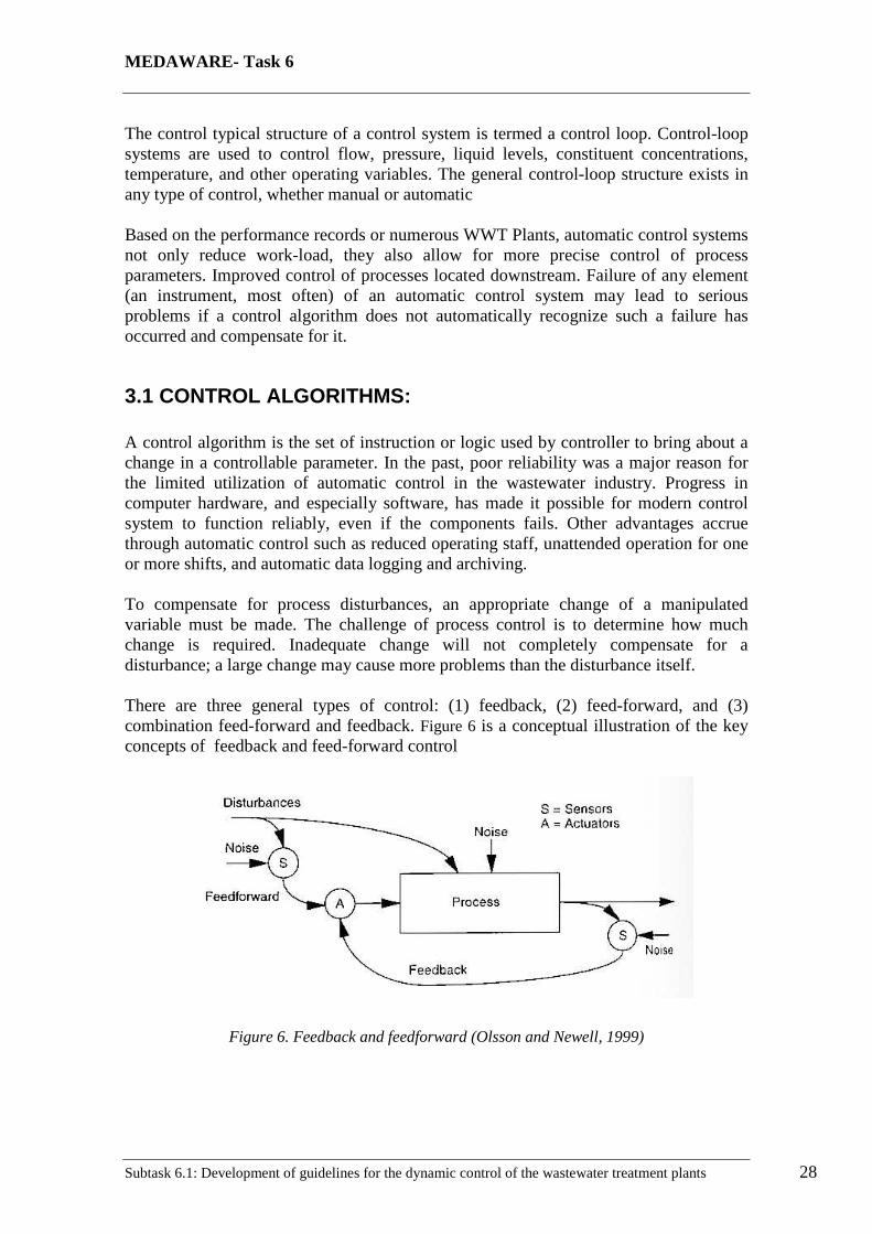
3.1 CONTROL ALGORITHMS: A control algorithm is the set of instruction or logic used by controller to bring about a change in a controllable parameter. In the past, poor reliability was a major reason for the limited utilization of automatic control in the wastewater industry. Progress in computer hardware, and especially software, has made it possible for modern control system to function reliably, even if the components fails. Other advantages accrue through automatic control such as reduced operating staff, unattended operation for one or more shifts, and automatic data logging and archiving. To compensate for process disturbances, an appropriate change of a manipulated variable must be made. The challenge of process control is to determine how much change is required. Inadequate change will not completely compensate for a disturbance; a large change may cause more problems than the disturbance itself. There are three general types of control: (1) feedback, (2) feed-forward, and (3) combination feed-forward and feedback. Figure 6 is a conceptual illustration of the key concepts of feedback and feed-forward control

Figure 6. Feedback and feedforward (Olsson and Newell, 1999)

MEDAWARE- Task 6


3.1.1 Feed-Forward Control: The feed-forward control method consists of measuring disturbances and changing manipulated parameters so that the controlled parameters will be maintained within a desires range. In the static feed-forward control algorithm, a manipulated parameter is calculated based on a linear relationship with a controlled variable, in more sophisticated dynamic feed-forward control algorithms, it is common practice to take into account process dynamics.

Unfortunately, most of the time measurements of disturbances as well as calculation of a required change in a manipulated parameter are very difficult task. As a result feed-forward control has limited application in the automation of WWT processes. The current-limited applications of feed-forward control include control of chemical addition and control of return activated-sludge flow from clarifiers to the aeration tanks. In Both cases, only one disturbances (influent flow change) is used for calculation of change in manipulated parameters. Because the effect of other disturbances(water-quality characteristics, for example) is not considered, a controlled parameter cannot be maintained within a narrow range. Development of advanced on-line water analyzers and computer modelling of WWT processes may help to make this type of control more feasible. Feedforward compensation is for example applied when the RAS of the WWTP is proportional to the incoming flow rate (ratio control). The goal of the control action is to maintain the sludge concentration in the aeration tank and therefore the biodegradation capacity nearly constant .MIMO control Multiple-input multiple-output (MIMO) allows the use of more than one input or output variable for the controller.

3.1.2 Feedback Control The principle of feedback control is one of the most intuitive concepts for process control. An action is taken to correct a less than desirable situation; the result of corrective action is then measured and a new correction action is applied. So instead of measuring a disturbance, a change in a controlled parameter is measured, and based on the measured change a manipulated parameter is calculated. There are several types of feedback control like on-off, proportional (P), proportional-derivative (PD), proportional-integral (PI), and proportional-integral-derivative (PID). Of these control modes, the most common are on-off and proportional-integral. Two types of control algorithms predominate in WWTP, indeed throughout the process industries in general are the On-off algorithm and the PID (Proportional-Integral-Derivative) algorithm.

• On-Off Agorithm

On-off is a crude way of automating open loop control. The main attractiveness of on-off control is that it is relay based with no apparent tuning difficulties and suffices for simple processes, which require only a crude level of control accuracy.

MEDAWARE- Task 6


In the on-off control the controlled variable will cycle up and down continuously (Figure 7). This is called limit cycling. The speed and amplitude of this cyclig depends on how fast the process responds to an on or off control action. Another aspect of this control is that it can create a disturbance to other parts of the process, not only forwards due to the limit cycling in the output, but also backwards due to the on-off switching of the input.

Figure 7. On-off Control example (Olsson and Newell, 1999)

• PID Agorithm PID controllers are the most common control in the industrial plants. It has been estimated that in some industrial applications more than 95% of the loops in a process plant will use PID. In the context of the time-varying, non-linear processes, optimal control performance cannot be expected from these controllers. However, the familiarity with concepts and properties of PID and on-off controllers has made their use very common. Typical formulation of the PID in the time domain is:

dt

deKdeKteKu DIpc ∫ ++= ττ )()(

The most intuitive features of PID, which can be justified by formal analysis, are as follows: (Katebi et al., 1999) Proportional Term (P):

- Increasing Kp ⇒ speed up the system response. - Increasing Kp ⇒ decreases any steady state offset in one exits. - Increasing Kp too much may saturate actuators. - The dynamical order of the closed loop system is the same as that of the

open loop system.

MEDAWARE- Task 6


Integral Term (I):

- The Integral term will almost exclusively be used in conjunction with P to give PI control.

- Integral control eliminates steady state offset. - Measurement bias must no exit otherwise this destroys the use or I

control to remove offsets. - PI control increases the dynamic order of the closed loop system thereby

introduces the potential for an unstable closed loop design. - PI control can cause excessive overshoot un the system response.

Derivative Term (D):

- The derivative term will always be used un a structure, which includes P to give PD control at least.

- The derivative term can be used to reduce response peaks, and effect the equivalent damping of a system. Rate feedback in motor control is a special form of PD control.

- Derivative control has no effect on steady state errors. - Pure derivative control will amplify the high frequency noise in a

measurement signal, hence it is usually implemented by a filtered form. - Derivative control does not effect the dynamic order or the closed loop

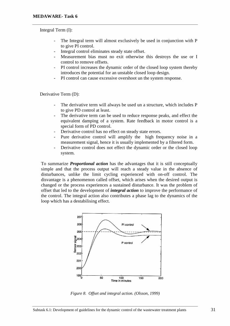
system. To summarize Proportional action has the advantages that it is still conceptually simple and that the process output will reach a steady value in the absence of disturbances, unlike the limit cycling experienced with on-off control. The disvantage is a phenomenon called offset, which arises when the desired output is changed or the process experiences a sustained disturbance. It was the problem of offset that led to the development of integral action to improve the performance of the control. The integral action also contributes a phase lag to the dynamics of the loop which has a destabilising effect.

Figure 8. Offset and integral action. (Olsson, 1999)

MEDAWARE- Task 6


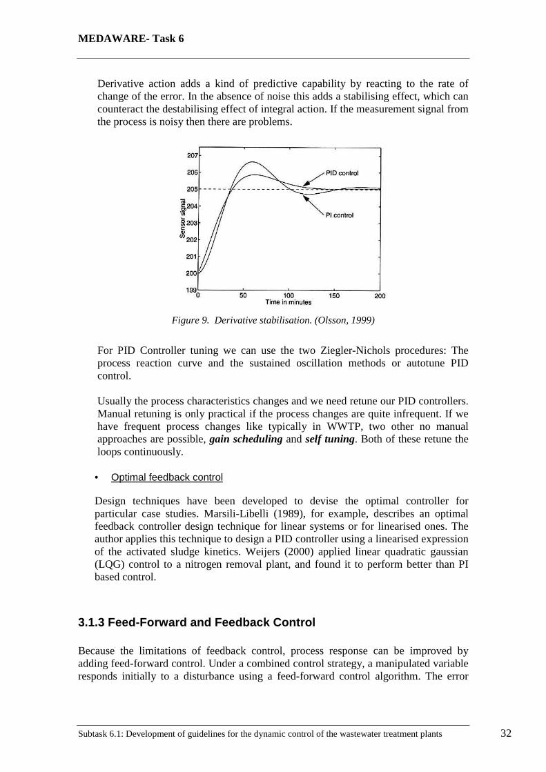
Derivative action adds a kind of predictive capability by reacting to the rate of change of the error. In the absence of noise this adds a stabilising effect, which can counteract the destabilising effect of integral action. If the measurement signal from the process is noisy then there are problems.

Figure 9. Derivative stabilisation. (Olsson, 1999)

For PID Controller tuning we can use the two Ziegler-Nichols procedures: The process reaction curve and the sustained oscillation methods or autotune PID control. Usually the process characteristics changes and we need retune our PID controllers. Manual retuning is only practical if the process changes are quite infrequent. If we have frequent process changes like typically in WWTP, two other no manual approaches are possible, gain scheduling and self tuning. Both of these retune the loops continuously.

• Optimal feedback control

Design techniques have been developed to devise the optimal controller for particular case studies. Marsili-Libelli (1989), for example, describes an optimal feedback controller design technique for linear systems or for linearised ones. The author applies this technique to design a PID controller using a linearised expression of the activated sludge kinetics. Weijers (2000) applied linear quadratic gaussian (LQG) control to a nitrogen removal plant, and found it to perform better than PI based control.

3.1.3 Feed-Forward and Feedback Control Because the limitations of feedback control, process response can be improved by adding feed-forward control. Under a combined control strategy, a manipulated variable responds initially to a disturbance using a feed-forward control algorithm. The error

MEDAWARE- Task 6


caused by inaccurate disturbance compensation is corrected by applying feedback PI control action. The combination control algorithms makes controller tuning more difficult and time-consuming because an additional tuning coefficient is required for feed-forward control action. As a result, this control combination is not used very often.

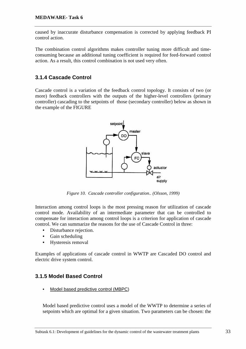
3.1.4 Cascade Control Cascade control is a variation of the feedback control topology. It consists of two (or more) feedback controllers with the outputs of the higher-level controllers (primary controller) cascading to the setpoints of those (secondary controller) below as shown in the example of the FIGURE

Figure 10. Cascade controller configuration.. (Olsson, 1999)

Interaction among control loops is the most pressing reason for utilization of cascade control mode. Availability of an intermediate parameter that can be controlled to compensate for interaction among control loops is a criterion for application of cascade control. We can summarize the reasons for the use of Cascade Control in three:

• Disturbance rejection. • Gain scheduling • Hysteresis removal

Examples of applications of cascade control in WWTP are Cascaded DO control and electric drive system control.

3.1.5 Model Based Control

• Model based predictive control (MBPC)

Model based predictive control uses a model of the WWTP to determine a series of setpoints which are optimal for a given situation. Two parameters can be chosen: the

MEDAWARE- Task 6


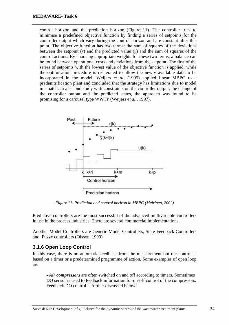
control horizon and the prediction horizon (Figure 11). The controller tries to minimise a predefined objective function by finding a series of setpoints for the controller output which vary during the control horizon and are constant after this point. The objective function has two terms: the sum of squares of the deviations between the setpoint (r) and the predicted value (y) and the sum of squares of the control actions. By choosing appropriate weights for these two terms, a balance can be found between operational costs and deviations from the setpoint. The first of the series of setpoints with the lowest value of the objective function is applied, while the optimisation procedure is re-iterated to allow the newly available data to be incorporated in the model. Weijers et al. (1995) applied linear MBPC to a predenitrification plant and concluded that the strategy has limitations due to model mismatch. In a second study with constraints on the controller output, the change of the controller output and the predicted states, the approach was found to be promising for a carousel type WWTP (Weijers et al., 1997).

Figure 11. Prediction and control horizon in MBPC (Meirlaen, 2002)

Predictive controllers are the most successful of the advanced multivariable controllers in use in the process industries. There are several commercial implementations. Another Model Controllers are Generic Model Controllers, State Feedback Controllers and Fuzzy controllers (Olsson, 1999)

3.1.6 Open Loop Control In this case, there is no automatic feedback from the measurement but the control is based on a timer or a predetermined programme of action. Some examples of open loop are:

- Air compressors are often switched on and off according to timers. Sometimes DO sensor is used to feedback information for on-off control of the compressors. Feedback DO control is further discussed below.

MEDAWARE- Task 6


- Sludge removal, particularly in primary sedimentation, is often based on timers instead of some sludge density or sludge blanket measurements. - Waste activated sludge pumping is often based on a timer. A better action is to base the wastage rate on conventional sludge age calculations. - Bar screen cleaning is sometimes based on a timer operation

3.1.7 Sequential Logical Control There are a number of applications involving sequences operations in any WWTP. Operations which proceed through a number of distinct steps in a set order depending on process conditions. Influent pump control and sand filter backwashing are typical examples. Actually this type of control is implemented in Programmable Logical Controllers (PLC). Microcomputers developed to sense on/off, handle Boolean operations, comparators and PID algorithms, activate on/off actuators and handle analog input and output signals. The logical decisions and calculations may be very simple in detail, but the decision chain in large plants are very complex. This naturally raises the demand for structuring the programming problem, its implementation and documentation. Ladder diagrams, which are simply relay system circuit diagrams, are being phased out of many automation systems but they are still commonly used to describe and document sequencing control implemented software. GRAFCET, now is an important and more sophisticated notation to describe binary sequences, including concurrent process.

Figure 12. Ladder logic diagram and GRAFCET diagram example for a batch tank (Olsson and Newell, 1999)

MEDAWARE- Task 6


The most common purely digital applications of sequencing involve the start-up and shutdown of more complex equipment. In a WWTP the lager air compressors, energy recovery equipment, grit and sludge handling equipment, and pumps can be applications in this category.

3.2 Control handles in WWTP control According to Schütze et al. (2002) three different control levels can be normally identified in the framework of treatment plants. At the highest level (overall level) the aim is the definition of overall operational objectives. At the second level (set point level), set points (possibly time-varying) of the individual controllers have to be determined. Finally, at the lowest level (controller level) the goal is the maintenance of set points usually with PID controllers. With regard to the set point level control, an overview of commonly controlled settings is given. (Meirlain, 2002; Olsson and Newell, 1999)

• Maximum inflow to WWTP One of the most applied control measures is the inflow regulation at WWTP. In almost all treatment plants it is normal behaviour to bypass flow above a certain threshold directly to the receiving water (Lessard and Beck, 1991). Several studies about the threshold variation have been carried out. The results for a rain event of short duration and high intensity showed a slight reduction in the overall suspended solids and COD mass discharged. For a long duration and low intensity storm the strategy eliminated the overflow almost entirely and improved the overall efficiency in terms of suspended solids and COD but, on the other hand, it aggravated the nitrification process.

• Filling and emptying of storm tanks Several control strategies can be developed with storm tanks. The storm tanks are usually filled by inflows exceeding the threshold of admitted flow to the WWTP. A current practice is to fill the tank and subsequently use it as a sedimentation basin. Another possibility is to fill the tank first and, once the storm tank is full, bypass the flow to the receiving water body. Alternatively, the storm tank can be filled in the early stages of the rain event and the following flow can be addressed to biological treatment (Lessard and Beck, 1991). Stricker (2000) looked at the effect of the emptying rate of storm tanks on WWTPs with a very low F/M ratio. Provided that sufficient aeration capacity is available, the treatment plant could handle up to 7 DWF (Dry Weather Flow) in flow rate. Bauwens et al. (1996) tested the effect of a storm tank in fill-and-bypass mode on the efficiency of the combined sewer-WWTP system. The storm tank was filled when the flow to the biological treatment exceeded 2.5 DWF and emptied when

MEDAWARE- Task 6


the flow fell below this value. It was found that especially the amount of suspended solids discharged could be reduced.

• Aeration Maintenance of a set point for DO in the activated sludge tank is the common control objective of the aeration system. It is important to find a good balance between a sufficient concentration of DO, that is strictly necessary for removal of carbonaceous material and for the nitrification process, and excessive oxygen supply, which results in high operational costs. Details can be found in Olsson and Newell (1999).

• Step feeding An interesting operational control is based on the step feed scheme. This strategy, that achieves an equalisation of the food to organisms ratio (F/M ratio) for the activated sludge, uses several inlet points to introduce the wastewater in the aeration tank. During wet weather the inlet point of the wastewater is placed near the middle or end of the tank, so that sludge may be stored at the head of the reactor. This measure reduces the suspended solids concentration in the feed to the secondary clarifier but also limits the nitrification process. Step feed control has been successfully used, e.g. by Lessard (1989) and Nyberg et al. (1996). Rouleau (1997) motivate the use of step feed control combined with the ratio control of the return activated sludge rate.

• Return activated sludge rate (RAS) Return of activated sludge to the aeration tank is fundamental for a good operation of the activated sludge process. The maintenance of a constant mixed liquor suspended solids (MLSS) concentration represents a common method of solids control. In steady state it is possible to calculate, by means of a mass balance, the return activated sludge ratio necessary to maintain a constant MLSS concentration. Another frequently applied method (Harremoës et al., 1993) consists of relating the return activated sludge to the WWTP inflow rate by a constant factor. In this case, the sludge rate is increased with increasing flow (ratio control). However, as this disturbs the settling process, Olsson and Newell (1999) propose an alternative in making the RAS proportional with the incoming flow to the settler. This has as a consequence that the sludge load to the settler is increased. Lessard (1989) proposed to increase the recycle rate to a predetermined value before or during the event and with this approach demonstrated an improvement of the WWTP effluent.

• Waste activate sludge rate (WAS) The sludge removal rate is determined by this parameter. If a sludge age and a MLSS concentration have to be maintained constant, it is possible, in steady state, to calculate the wastage rate. By means of a mass balance, the wastage rate can be computed taking into account the MLSS concentration in the aeration tank and the MLSS concentration in the effluent and in the underflow. However, the total mass of sludge in the system is

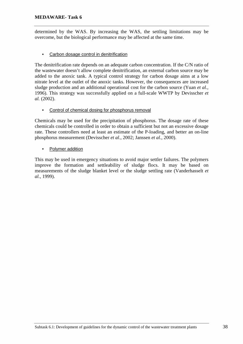
MEDAWARE- Task 6


determined by the WAS. By increasing the WAS, the settling limitations may be overcome, but the biological performance may be affected at the same time.

• Carbon dosage control in denitrification The denitrification rate depends on an adequate carbon concentration. If the C/N ratio of the wastewater doesn’t allow complete denitrification, an external carbon source may be added to the anoxic tank. A typical control strategy for carbon dosage aims at a low nitrate level at the outlet of the anoxic tanks. However, the consequences are increased sludge production and an additional operational cost for the carbon source (Yuan et al., 1996). This strategy was successfully applied on a full-scale WWTP by Devisscher et al. (2002).

• Control of chemical dosing for phosphorus removal Chemicals may be used for the precipitation of phosphorus. The dosage rate of these chemicals could be controlled in order to obtain a sufficient but not an excessive dosage rate. These controllers need at least an estimate of the P-loading, and better an on-line phosphorus measurement (Devisscher et al., 2002; Janssen et al., 2000).

• Polymer addition This may be used in emergency situations to avoid major settler failures. The polymers improve the formation and settleability of sludge flocs. It may be based on measurements of the sludge blanket level or the sludge settling rate (Vanderhasselt et al., 1999).

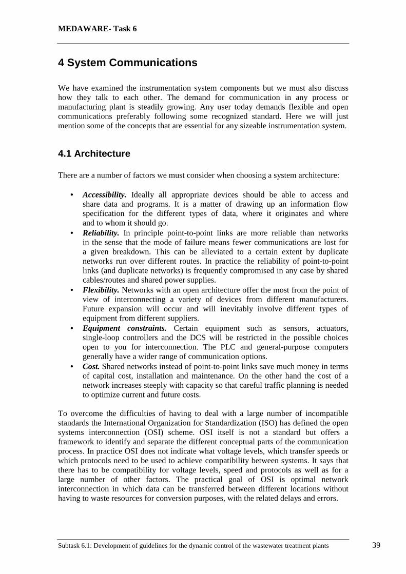
MEDAWARE- Task 6


4 System Communications We have examined the instrumentation system components but we must also discuss how they talk to each other. The demand for communication in any process or manufacturing plant is steadily growing. Any user today demands flexible and open communications preferably following some recognized standard. Here we will just mention some of the concepts that are essential for any sizeable instrumentation system.

4.1 Architecture There are a number of factors we must consider when choosing a system architecture:

• Accessibility. Ideally all appropriate devices should be able to access and share data and programs. It is a matter of drawing up an information flow specification for the different types of data, where it originates and where and to whom it should go.

• Reliability. In principle point-to-point links are more reliable than networks in the sense that the mode of failure means fewer communications are lost for a given breakdown. This can be alleviated to a certain extent by duplicate networks run over different routes. In practice the reliability of point-to-point links (and duplicate networks) is frequently compromised in any case by shared cables/routes and shared power supplies.

• Flexibility. Networks with an open architecture offer the most from the point of view of interconnecting a variety of devices from different manufacturers. Future expansion will occur and will inevitably involve different types of equipment from different suppliers.

• Equipment constraints. Certain equipment such as sensors, actuators, single-loop controllers and the DCS will be restricted in the possible choices open to you for interconnection. The PLC and general-purpose computers generally have a wider range of communication options.

• Cost. Shared networks instead of point-to-point links save much money in terms of capital cost, installation and maintenance. On the other hand the cost of a network increases steeply with capacity so that careful traffic planning is needed to optimize current and future costs.

To overcome the difficulties of having to deal with a large number of incompatible standards the International Organization for Standardization (ISO) has defined the open systems interconnection (OSI) scheme. OSI itself is not a standard but offers a framework to identify and separate the different conceptual parts of the communication process. In practice OSI does not indicate what voltage levels, which transfer speeds or which protocols need to be used to achieve compatibility between systems. It says that there has to be compatibility for voltage levels, speed and protocols as well as for a large number of other factors. The practical goal of OSI is optimal network interconnection in which data can be transferred between different locations without having to waste resources for conversion purposes, with the related delays and errors.

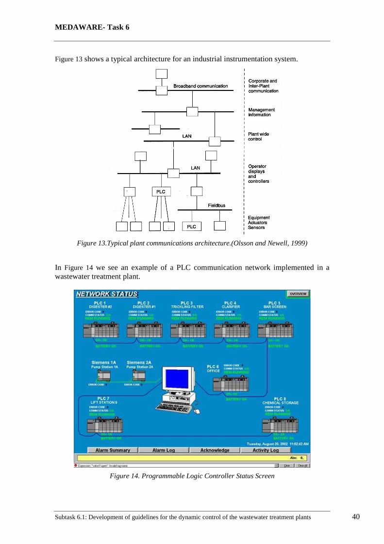
MEDAWARE- Task 6


Figure 13 shows a typical architecture for an industrial instrumentation system.

Figure 13.Typical plant communications architecture.(Olsson and Newell, 1999)

In Figure 14 we see an example of a PLC communication network implemented in a wastewater treatment plant.

Figure 14. Programmable Logic Controller Status Screen

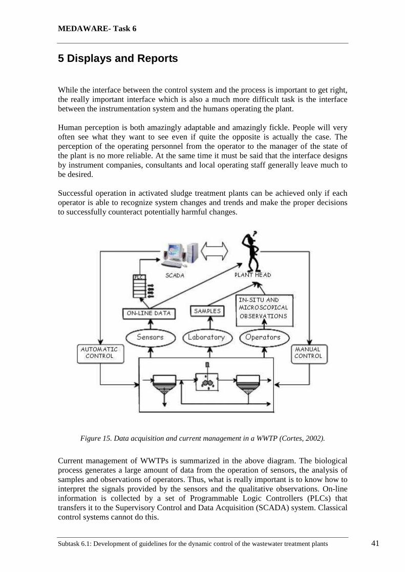
MEDAWARE- Task 6


5 Displays and Reports While the interface between the control system and the process is important to get right, the really important interface which is also a much more difficult task is the interface between the instrumentation system and the humans operating the plant. Human perception is both amazingly adaptable and amazingly fickle. People will very often see what they want to see even if quite the opposite is actually the case. The perception of the operating personnel from the operator to the manager of the state of the plant is no more reliable. At the same time it must be said that the interface designs by instrument companies, consultants and local operating staff generally leave much to be desired. Successful operation in activated sludge treatment plants can be achieved only if each operator is able to recognize system changes and trends and make the proper decisions to successfully counteract potentially harmful changes.

Figure 15. Data acquisition and current management in a WWTP (Cortes, 2002).

Current management of WWTPs is summarized in the above diagram. The biological process generates a large amount of data from the operation of sensors, the analysis of samples and observations of operators. Thus, what is really important is to know how to interpret the signals provided by the sensors and the qualitative observations. On-line information is collected by a set of Programmable Logic Controllers (PLCs) that transfers it to the Supervisory Control and Data Acquisition (SCADA) system. Classical control systems cannot do this.

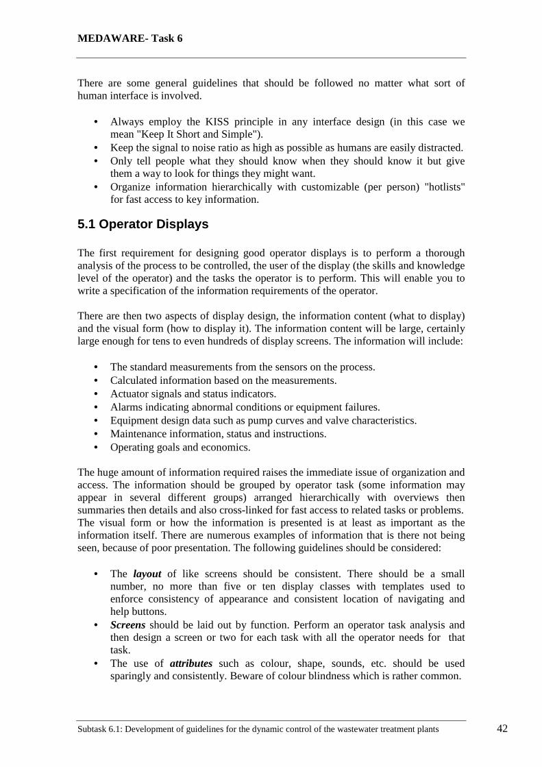
MEDAWARE- Task 6


There are some general guidelines that should be followed no matter what sort of human interface is involved.

• Always employ the KISS principle in any interface design (in this case we mean "Keep It Short and Simple").

• Keep the signal to noise ratio as high as possible as humans are easily distracted. • Only tell people what they should know when they should know it but give

them a way to look for things they might want. • Organize information hierarchically with customizable (per person) "hotlists"

for fast access to key information.

5.1 Operator Displays The first requirement for designing good operator displays is to perform a thorough analysis of the process to be controlled, the user of the display (the skills and knowledge level of the operator) and the tasks the operator is to perform. This will enable you to write a specification of the information requirements of the operator. There are then two aspects of display design, the information content (what to display) and the visual form (how to display it). The information content will be large, certainly large enough for tens to even hundreds of display screens. The information will include:

• The standard measurements from the sensors on the process. • Calculated information based on the measurements. • Actuator signals and status indicators. • Alarms indicating abnormal conditions or equipment failures. • Equipment design data such as pump curves and valve characteristics. • Maintenance information, status and instructions. • Operating goals and economics.

The huge amount of information required raises the immediate issue of organization and access. The information should be grouped by operator task (some information may appear in several different groups) arranged hierarchically with overviews then summaries then details and also cross-linked for fast access to related tasks or problems. The visual form or how the information is presented is at least as important as the information itself. There are numerous examples of information that is there not being seen, because of poor presentation. The following guidelines should be considered:

• The layout of like screens should be consistent. There should be a small number, no more than five or ten display classes with templates used to enforce consistency of appearance and consistent location of navigating and help buttons.

• Screens should be laid out by function. Perform an operator task analysis and then design a screen or two for each task with all the operator needs for that task.

• The use of attributes such as colour, shape, sounds, etc. should be used sparingly and consistently. Beware of colour blindness which is rather common.

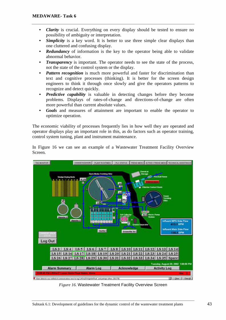
MEDAWARE- Task 6


• Clarity is crucial. Everything on every display should be tested to ensure no possibility of ambiguity or interpretation.

• Simplicity is a key word. It is better to use three simple clear displays than one cluttered and confusing display.

• Redundancy of information is the key to the operator being able to validate abnormal behavior.

• Transparency is important. The operator needs to see the state of the process, not the state of the control system or the display.

• Pattern recognition is much more powerful and faster for discrimination than text and cognitive processes (thinking). It is better for the screen design engineers to think it through once slowly and give the operators patterns to recognize and detect quickly.

• Predictive capability is valuable in detecting changes before they become problems. Displays of rates-of-change and directions-of-change are often more powerful than current absolute values.

• Goals and measures of attainment are important to enable the operator to optimize operation.

The economic viability of processes frequently lies in how well they are operated and operator displays play an important role in this, as do factors such as operator training, control system tuning, plant and instrument maintenance. In Figure 16 we can see an example of a Wastewater Treatment Facility Overview Screen.

Figure 16. Wastewater Treatment Facility Overview Screen

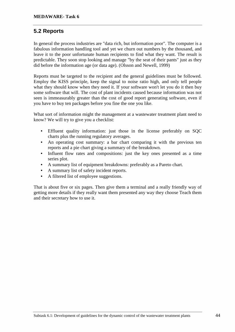
MEDAWARE- Task 6


5.2 Reports In general the process industries are "data rich, but information poor". The computer is a fabulous information handling tool and yet we churn out numbers by the thousand, and leave it to the poor unfortunate human recipients to find what they want. The result is predictable. They soon stop looking and manage "by the seat of their pants" just as they did before the information age (or data age). (Olsson and Newell, 1999) Reports must be targeted to the recipient and the general guidelines must be followed. Employ the KISS principle, keep the signal to noise ratio high, and only tell people what they should know when they need it. If your software won't let you do it then buy some software that will. The cost of plant incidents caused because information was not seen is immeasurably greater than the cost of good report generating software, even if you have to buy ten packages before you fine the one you like. What sort of information might the management at a wastewater treatment plant need to know? We will try to give you a checklist:

• Effluent quality information: just those in the license preferably on SQC charts plus the running regulatory averages.

• An operating cost summary: a bar chart comparing it with the previous ten reports and a pie chart giving a summary of the breakdown.

• Influent flow rates and compositions: just the key ones presented as a time series plot.

• A summary list of equipment breakdowns: preferably as a Pareto chart. • A summary list of safety incident reports. • A filtered list of employee suggestions.

That is about five or six pages. Then give them a terminal and a really friendly way of getting more details if they really want them presented any way they choose Teach them and their secretary how to use it.

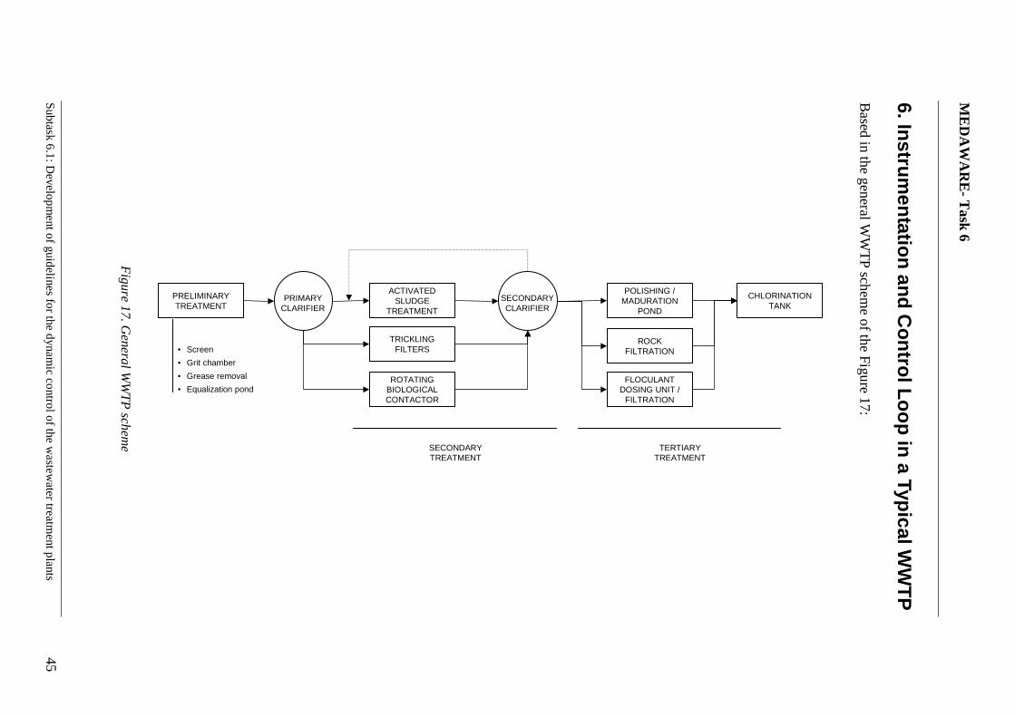
ME

DA

WA

RE

- Task 6

Sub

task 6.1

: Develo

pm

ent o

f guideline

s for the d

ynam

ic contro

l of the w

aste

water treatm

ent plants

45

6. Instru

men

tation

and

Co

ntro

l Lo

op

in a Typ

ical WW

TP

B

ased in the general WW

TP

scheme of the F

igure 17:

PRELIMINARYTREATMENT

ACTIVATEDSLUDGE

TREATMENT

SECONDARYCLARIFIER

PRIMARYCLARIFIER

• Screen

• Grit chamber

• Grease removal

• Equalization pond

TRICKLINGFILTERS

POLISHING /MADURATION

POND

ROCKFILTRATION

ROTATINGBIOLOGICALCONTACTOR

FLOCULANTDOSING UNIT /

FILTRATION

CHLORINATIONTANK

SECONDARYTREATMENT

TERTIARYTREATMENT

Figure 17. G

eneral WW

TP

scheme

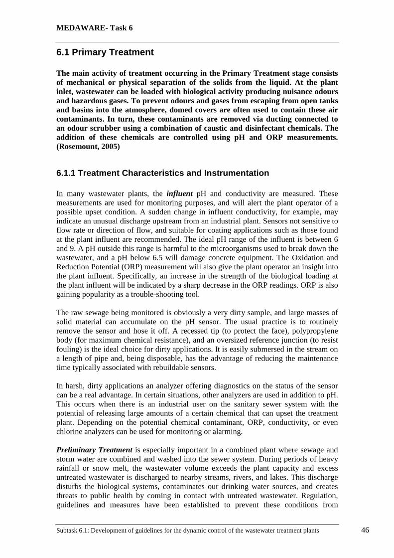
MEDAWARE- Task 6


6.1 Primary Treatment

The main activity of treatment occurring in the Primary Treatment stage consists of mechanical or physical separation of the solids from the liquid. At the plant inlet, wastewater can be loaded with biological activity producing nuisance odours and hazardous gases. To prevent odours and gases from escaping from open tanks and basins into the atmosphere, domed covers are often used to contain these air contaminants. In turn, these contaminants are removed via ducting connected to an odour scrubber using a combination of caustic and disinfectant chemicals. The addition of these chemicals are controlled using pH and ORP measurements. (Rosemount, 2005)

6.1.1 Treatment Characteristics and Instrumentation In many wastewater plants, the influent pH and conductivity are measured. These measurements are used for monitoring purposes, and will alert the plant operator of a possible upset condition. A sudden change in influent conductivity, for example, may indicate an unusual discharge upstream from an industrial plant. Sensors not sensitive to flow rate or direction of flow, and suitable for coating applications such as those found at the plant influent are recommended. The ideal pH range of the influent is between 6 and 9. A pH outside this range is harmful to the microorganisms used to break down the wastewater, and a pH below 6.5 will damage concrete equipment. The Oxidation and Reduction Potential (ORP) measurement will also give the plant operator an insight into the plant influent. Specifically, an increase in the strength of the biological loading at the plant influent will be indicated by a sharp decrease in the ORP readings. ORP is also gaining popularity as a trouble-shooting tool. The raw sewage being monitored is obviously a very dirty sample, and large masses of solid material can accumulate on the pH sensor. The usual practice is to routinely remove the sensor and hose it off. A recessed tip (to protect the face), polypropylene body (for maximum chemical resistance), and an oversized reference junction (to resist fouling) is the ideal choice for dirty applications. It is easily submersed in the stream on a length of pipe and, being disposable, has the advantage of reducing the maintenance time typically associated with rebuildable sensors. In harsh, dirty applications an analyzer offering diagnostics on the status of the sensor can be a real advantage. In certain situations, other analyzers are used in addition to pH. This occurs when there is an industrial user on the sanitary sewer system with the potential of releasing large amounts of a certain chemical that can upset the treatment plant. Depending on the potential chemical contaminant, ORP, conductivity, or even chlorine analyzers can be used for monitoring or alarming. Preliminary Treatment is especially important in a combined plant where sewage and storm water are combined and washed into the sewer system. During periods of heavy rainfall or snow melt, the wastewater volume exceeds the plant capacity and excess untreated wastewater is discharged to nearby streams, rivers, and lakes. This discharge disturbs the biological systems, contaminates our drinking water sources, and creates threats to public health by coming in contact with untreated wastewater. Regulation, guidelines and measures have been established to prevent these conditions from

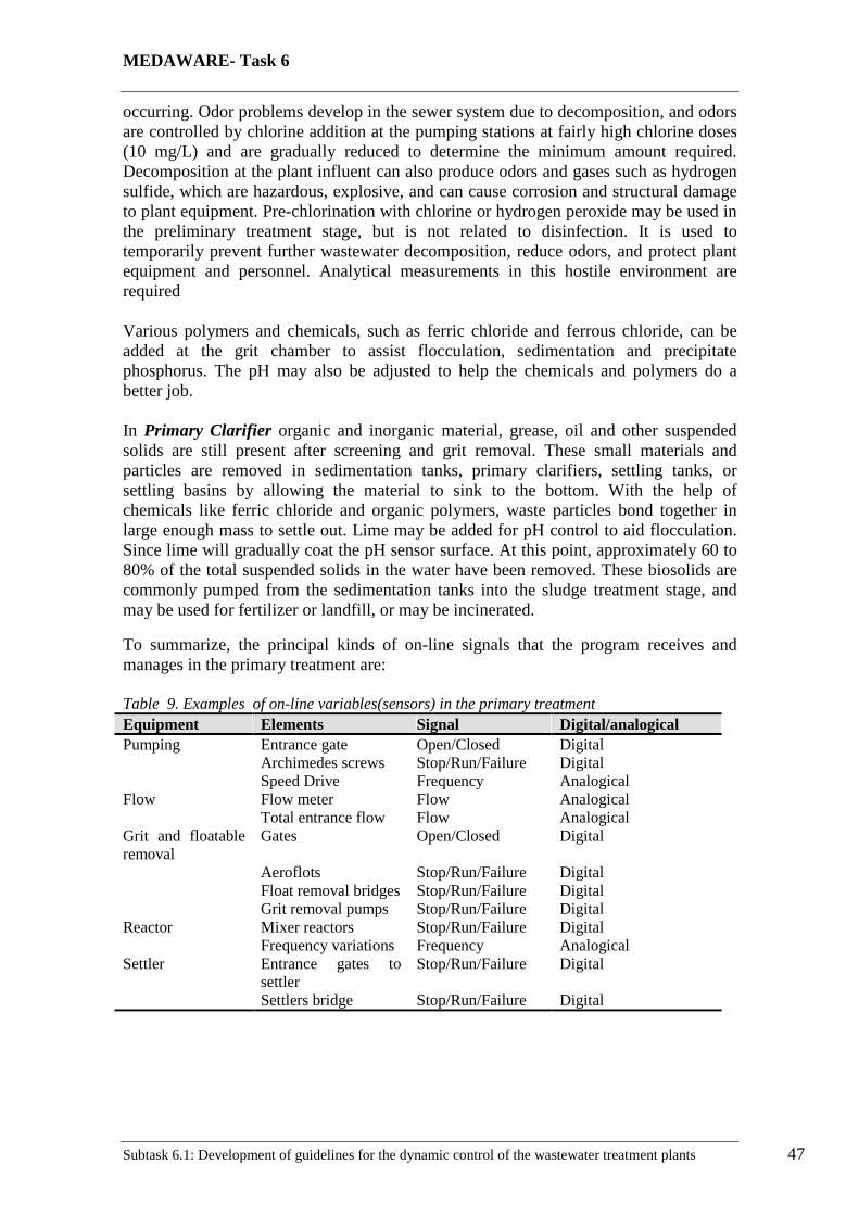
MEDAWARE- Task 6


occurring. Odor problems develop in the sewer system due to decomposition, and odors are controlled by chlorine addition at the pumping stations at fairly high chlorine doses (10 mg/L) and are gradually reduced to determine the minimum amount required. Decomposition at the plant influent can also produce odors and gases such as hydrogen sulfide, which are hazardous, explosive, and can cause corrosion and structural damage to plant equipment. Pre-chlorination with chlorine or hydrogen peroxide may be used in the preliminary treatment stage, but is not related to disinfection. It is used to temporarily prevent further wastewater decomposition, reduce odors, and protect plant equipment and personnel. Analytical measurements in this hostile environment are required Various polymers and chemicals, such as ferric chloride and ferrous chloride, can be added at the grit chamber to assist flocculation, sedimentation and precipitate phosphorus. The pH may also be adjusted to help the chemicals and polymers do a better job. In Primary Clarifier organic and inorganic material, grease, oil and other suspended solids are still present after screening and grit removal. These small materials and particles are removed in sedimentation tanks, primary clarifiers, settling tanks, or settling basins by allowing the material to sink to the bottom. With the help of chemicals like ferric chloride and organic polymers, waste particles bond together in large enough mass to settle out. Lime may be added for pH control to aid flocculation. Since lime will gradually coat the pH sensor surface. At this point, approximately 60 to 80% of the total suspended solids in the water have been removed. These biosolids are commonly pumped from the sedimentation tanks into the sludge treatment stage, and may be used for fertilizer or landfill, or may be incinerated. To summarize, the principal kinds of on-line signals that the program receives and manages in the primary treatment are: Table 9. Examples of on-line variables(sensors) in the primary treatment Equipment Elements Signal Digital/analogical Pumping Entrance gate Open/Closed Digital Archimedes screws Stop/Run/Failure Digital Speed Drive Frequency Analogical Flow Flow meter Flow Analogical Total entrance flow Flow Analogical Grit and floatable removal

Gates Open/Closed Digital

Aeroflots Stop/Run/Failure Digital Float removal bridges Stop/Run/Failure Digital Grit removal pumps Stop/Run/Failure Digital Reactor Mixer reactors Stop/Run/Failure Digital Frequency variations Frequency Analogical Settler Entrance gates to

settler Stop/Run/Failure Digital

Settlers bridge Stop/Run/Failure Digital

MEDAWARE- Task 6


6.1.2 Control Loop in Primary Treatment Flow Linearization A constant inflow is required to achieve a good biological process operation. However, the real inflow to the plant is non-linear. The inflow linearization is achieved by means of the primary settlers. Whenever the real inflow to the plant is greater than an average inflow, overflow is accumulated in a settler. In contrast, whenever the inflow is less than an average inflow, the flow is supplemented with water accumulated in the settler. It is very difficult to determine the average value. In some WWTP, there are a knowledge-based programs used to get a more lineal inflow profile. The program determines the average value from the current time and the actual WWTP inflow. The average value is used as a set-point for the control loop (i.e. cascade controlling). The process value is measured by a sensor and the actuator of a control loop is a gate.

Figure 18. Flow Linearization Control Diagram (Cortes, 2002)

By-pass There is an upper limitation of the inflow to the biological reactor. The maximum possible inflow is realised by a gate; the overflow is directly by-passed to the river. Process value is measured by a flow meter, the set-point value is given by an expert (the head of the plant). By-passed flow is measured by another flow meter. Small faults of the control loops could be corrected by any next control loop, but at the expense of increasing operating costs. Extreme faults are very dangerous and have to be repaired as soon as possible.

MEDAWARE- Task 6


Figure 19. By-pass Control Diagram (Cortes, 2002)

6.2 Secondary Treatment Secondary treatment removes up to 85% of the remaining organic material through a biological process by cultivating and adding sewage microorganisms to the wastewater. This process is accomplished in a trickling filter or an aeration tank. A trickling filter uses a bed of stones or pieces of corrugated plastic media. As sewage is passed through these beds, microorganisms such as bacteria and protozoa gather on surfaces, multiply and consume most of the organic matter. (Rosemount, 2005)

6.2.1 Treatment Characteristics and Instrumentation After leaving the primary treatment stage, sewage is pumped into aeration tanks. The sludge is loaded with microorganisms and mixed with air or pure oxygen. As air is forced into the aeration basins, it increases the activity of these microorganisms and helps keep the organic waste thoroughly mixed. Dissolved oxygen (DO) is added to the aeration basin to enhance the oxidation process by providing oxygen to aerobic microorganisms so they can successfully turn organic wastes into inorganic by products, specifically carbon dioxide, water and sludge, which may contain nitrated phosphates, sulfates and highly active bacteria. Stated simply, there are two main categories of microorganisms (“bugs”) that digest waste—carbon eaters (carbonaceous) and ammonia eaters (nitrogenous)—and both of these groups need oxygen to reproduce and sustain life. In order to metabolize food and reproduce, each bug must have at least 0.1 to 0.3 mg/L DO. Most plants maintain about 2 mg/L of DO so the bugs contained inside the floc can also get oxygen. If the DO is less than 2 mg/L, the bugs in the center may die since the bugs on the outside of the floc use up the DO first. If this happens, the floc breaks up.

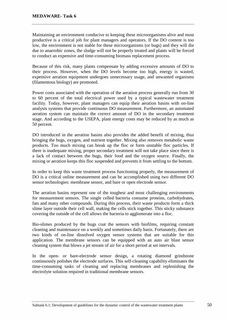
MEDAWARE- Task 6


Maintaining an environment conducive to keeping these microorganisms alive and most productive is a critical job for plant managers and operators. If the DO content is too low, the environment is not stable for these microorganisms (or bugs) and they will die due to anaerobic zones, the sludge will not be properly treated and plants will be forced to conduct an expensive and time-consuming biomass replacement process. Because of this risk, many plants compensate by adding excessive amounts of DO to their process. However, when the DO levels become too high, energy is wasted, expensive aeration equipment undergoes unnecessary usage, and unwanted organisms (filamentous biology) are promoted. Power costs associated with the operation of the aeration process generally run from 30 to 60 percent of the total electrical power used by a typical wastewater treatment facility. Today, however, plant managers can equip their aeration basins with on-line analysis systems that provide continuous DO measurement. Furthermore, an automated aeration system can maintain the correct amount of DO in the secondary treatment stage. And according to the USEPA, plant energy costs may be reduced by as much as 50 percent. DO introduced in the aeration basins also provides the added benefit of mixing, thus bringing the bugs, oxygen, and nutrient together. Mixing also removes metabolic waste products. Too much mixing can break up the floc or form unstable floc particles. If there is inadequate mixing, proper secondary treatment will not take place since there is a lack of contact between the bugs, their food and the oxygen source. Finally, the mixing or aeration keeps this floc suspended and prevents it from settling to the bottom. In order to keep this waste treatment process functioning properly, the measurement of DO is a critical online measurement and can be accomplished using two different DO sensor technologies: membrane sensor, and bare or open electrode sensor. The aeration basins represent one of the toughest and most challenging environments for measurement sensors. The single celled bacteria consume proteins, carbohydrates, fats and many other compounds. During this process, their waste products form a thick slime layer outside their cell wall, making the cells stick together. This sticky substance covering the outside of the cell allows the bacteria to agglomerate into a floc. Bio-slimes produced by the bugs coat the sensors with biofilms, requiring constant cleaning and maintenance on a weekly and sometimes daily basis. Fortunately, there are two kinds of on-line dissolved oxygen sensor systems that are suitable for this application. The membrane sensors can be equipped with an auto air blast sensor cleaning system that blows a jet stream of air for a short period at set intervals. In the open- or bare-electrode sensor design, a rotating diamond grindstone continuously polishes the electrode surfaces. This self-cleaning capability eliminates the time-consuming tasks of cleaning and replacing membranes and replenishing the electrolyte solution required in traditional membrane sensors.

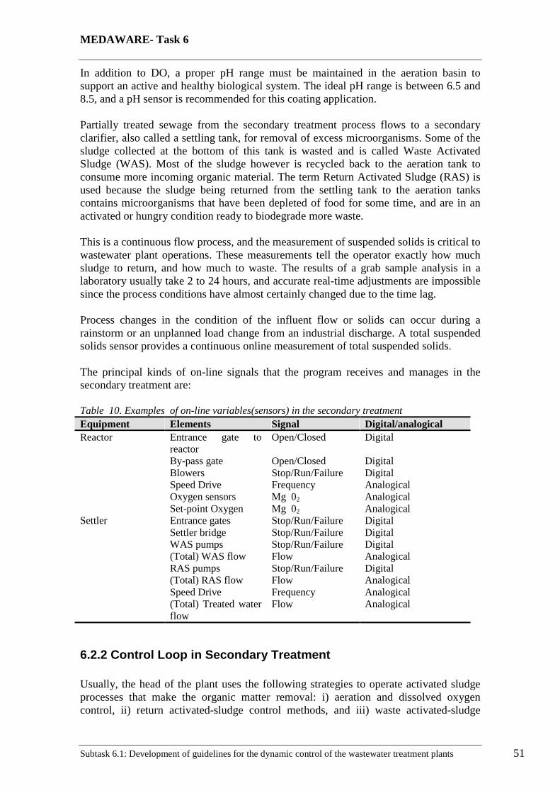
MEDAWARE- Task 6


In addition to DO, a proper pH range must be maintained in the aeration basin to support an active and healthy biological system. The ideal pH range is between 6.5 and 8.5, and a pH sensor is recommended for this coating application. Partially treated sewage from the secondary treatment process flows to a secondary clarifier, also called a settling tank, for removal of excess microorganisms. Some of the sludge collected at the bottom of this tank is wasted and is called Waste Activated Sludge (WAS). Most of the sludge however is recycled back to the aeration tank to consume more incoming organic material. The term Return Activated Sludge (RAS) is used because the sludge being returned from the settling tank to the aeration tanks contains microorganisms that have been depleted of food for some time, and are in an activated or hungry condition ready to biodegrade more waste. This is a continuous flow process, and the measurement of suspended solids is critical to wastewater plant operations. These measurements tell the operator exactly how much sludge to return, and how much to waste. The results of a grab sample analysis in a laboratory usually take 2 to 24 hours, and accurate real-time adjustments are impossible since the process conditions have almost certainly changed due to the time lag. Process changes in the condition of the influent flow or solids can occur during a rainstorm or an unplanned load change from an industrial discharge. A total suspended solids sensor provides a continuous online measurement of total suspended solids. The principal kinds of on-line signals that the program receives and manages in the secondary treatment are: Table 10. Examples of on-line variables(sensors) in the secondary treatment Equipment Elements Signal Digital/analogical Reactor Entrance gate to

reactor Open/Closed Digital

By-pass gate Open/Closed Digital Blowers Stop/Run/Failure Digital Speed Drive Frequency Analogical Oxygen sensors Mg 02 Analogical Set-point Oxygen Mg 02 Analogical Settler Entrance gates Stop/Run/Failure Digital Settler bridge Stop/Run/Failure Digital WAS pumps Stop/Run/Failure Digital (Total) WAS flow Flow Analogical RAS pumps Stop/Run/Failure Digital (Total) RAS flow Flow Analogical Speed Drive Frequency Analogical (Total) Treated water

flow Flow Analogical

6.2.2 Control Loop in Secondary Treatment Usually, the head of the plant uses the following strategies to operate activated sludge processes that make the organic matter removal: i) aeration and dissolved oxygen control, ii) return activated-sludge control methods, and iii) waste activated-sludge

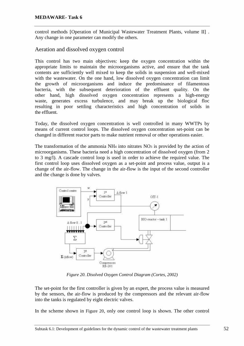
MEDAWARE- Task 6


control methods [Operation of Municipal Wastewater Treatment Plants, volume II] . Any change in one parameter can modify the others. Aeration and dissolved oxygen control This control has two main objectives: keep the oxygen concentration within the appropriate limits to maintain the microorganisms active, and ensure that the tank contents are sufficiently well mixed to keep the solids in suspension and well-mixed with the wastewater. On the one hand, low dissolved oxygen concentration can limit the growth of microorganisms and induce the predominance of filamentous bacteria, with the subsequent deterioration of the effluent quality. On the other hand, high dissolved oxygen concentration represents a high-energy waste, generates excess turbulence, and may break up the biological floc resulting in poor settling characteristics and high concentration of solids in the effluent.

Today, the dissolved oxygen concentration is well controlled in many WWTPs by means of current control loops. The dissolved oxygen concentration set-point can be changed in different reactor parts to make nutrient removal or other operations easier. The transformation of the ammonia NH4 into nitrates NO3 is provided by the action of microorganisms. These bacteria need a high concentration of dissolved oxygen (from 2 to 3 mg/l). A cascade control loop is used in order to achieve the required value. The first control loop uses dissolved oxygen as a set-point and process value, output is a change of the air-flow. The change in the air-flow is the input of the second controller and the change is done by valves.

Figure 20. Disolved Oxygen Control Diagram (Cortes, 2002)

The set-point for the first controller is given by an expert, the process value is measured by the sensors, the air-flow is produced by the compressors and the relevant air-flow into the tanks is regulated by eight electric valves. In the scheme shown in Figure 20, only one control loop is shown. The other control

MEDAWARE- Task 6


loops are similar. Faults at the control loop are very dangerous. Lack of dissolved oxygen leads to a decrease in the nitrification phase efficiency and there is ammonia in the treated water. An excess of dissolved oxygen leads to an increase in the abundance of microorganisms that appear in the treated water. Return activated sludge control This control allow maintaining a suitable contraction of the mixed liquor, which keeps the activated-sludge process operating properly.

A percentage of the MLSS settled in the clarifier is returned back to the reactor as RAS. This action allows keeping the right concentration of microorganisms in the aeration tanks to biologically treat the wastewater. The return sludge flow rate has to be well calculated to avoid the different solids concentrations between operation units and other operational problems. There are three ways to return sludge to the reactor, by means of a constant rate, a constant percentage of secondary influent flow, and a varying rate to optimise the concentration and retention time of clarifier solids. There are different RAS control techniques: direct sludge blanket level control, settleability, secondary clarifier mass balance, aeration tank mass balance, and sludge quality.

Figure 21 Sludge Recirculation Control Diagram (Cortes, 2002)

The extra sludge in the secondary settlers is again used in the biological reactors. Sludge recirculation is provided by pumps. The process value is measured by a flow meter, while the set-point is given by a set-point algorithm (cascade controlling). The algorithm computes the set-point from: a) Inflow to the plant b) SVI - Sludge Volume Index given by a laboratory

MEDAWARE- Task 6


Sludge recirculation plays a key role in the treatment process; it allows the return of nitrates to the reactor for the denitrification phase. Small faults in the control loop can be corrected by the sludge removal control loop 3, but at the expense of an increase in the operating costs and a decrease in the treated water quality. An extreme fault has to be solved as soon as possible - excess of recirculated sludge leads to a large amount of microorganisms in the treated water; failure to recirculate leads to failure of the denitrification phase (presence of nitrates in the treated water). Waste activated sludge control WAS control are the most important techniques to control the solids inventory in the system. The wasting rate (WAS) is used to control the solids. The wasting of sludge affects the system more than any other process control adjustment. It can affect effluent quality, the microorganisms growth rate and types, oxygen consumption, mixed liquor settleability, nutrient quantities needed, the occurrence of foaming and the possibility of nitrification. There are four methods to effect WAS control: constant Sludge Residence Time (SRT), constant F/M ratio, constant MLSS, and sludge quality.

Figure 22.Sludge Removal Control Diagram. (Corte, .2002)

In the example of Figure 22, a specific amount of MLSS is required for a good reactor function; whenever it does not work well, excess of sludge is removed. The set-point for the controller (the MLSS amount) is given by an expert (head of the plant), the process value is measured by an MLSS sensor and the excess of sludge is removed by a pair of pumps. Errors in the control loop can be corrected by the RAS control, but at the expense of an increase in the operating costs and a decrease in the treated water quality.

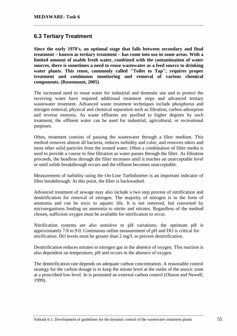
MEDAWARE- Task 6


6.3 Tertiary Treatment Since the early 1970's, an optional stage that falls between secondary and final treatment – known as tertiary treatment – has come into use in some areas. With a limited amount of usable fresh water, combined with the contamination of water sources, there is sometimes a need to reuse wastewater as a feed source to drinking water plants. This reuse, commonly called "Toilet to Tap", requires proper treatment and continuous monitoring and removal of various chemical components. (Rosemount, 2005) The increased need to reuse water for industrial and domestic use and to protect the receiving water have required additional treatment steps and advanced tertiary wastewater treatment. Advanced waste treatment techniques include phosphorus and nitrogen removal, physical and chemical separation such as filtration, carbon adsorption and reverse osmosis. As waste effluents are purified to higher degrees by such treatment, the effluent water can be used for industrial, agricultural, or recreational purposes. Often, treatment consists of passing the wastewater through a filter medium. This method removes almost all bacteria, reduces turbidity and color, and removes odors and most other solid particles from the treated water. Often a combination of filter media is used to provide a course to fine filtration as water passes through the filter. As filtration proceeds, the headloss through the filter increases until it reaches an unacceptable level or until solids breakthrough occurs and the effluent becomes unacceptable. Measurement of turbidity using the On-Line Turbidimeter is an important indicator of filter breakthrough. At this point, the filter is backwashed. Advanced treatment of sewage may also include a two step process of nitrification and denitrification for removal of nitrogen. The majority of nitrogen is in the form of ammonia and can be toxic to aquatic life. It is not removed, but converted by microorganisms feeding on ammonia to nitrite and nitrates. Regardless of the method chosen, sufficient oxygen must be available for nitrification to occur. Nitrification systems are also sensitive to pH variations; the optimum pH is approximately 7.8 to 9.0. Continuous online measurement of pH and DO is critical for nitrification. DO levels must be greater than 2 mg/L to prevent denitrification. Denitrification reduces nitrates to nitrogen gas in the absence of oxygen. This reaction is also dependent on temperature, pH and occurs in the absence of oxygen. The denitrification rate depends on adequate carbon concentration. A reasonable control strategy for the carbon dosage is to keep the nitrate level at the outlet of the anoxic zone at a prescribed low level. In is presented an external carbon control (Olsson and Newell, 1999).

MEDAWARE- Task 6


Figure 23.External Carbon control with feedback and feedforward. (Olsson and Newell, 1999)

6.4 Final Treatment In the final stage of wastewater treatment, disinfectants are added to kill disease-causing organisms and microorganisms used in the treatment process. Disinfection inactivates or destroys pathogenic organisms and prevents the spread of waterborne diseases to downstream users and the environment. A common disinfectant is chlorine gas, but most of municipalities manufacture their own chlorine solution such as sodium hypochlorite. Chlorine dosages ranging from 5 to 20 mg/L kill 99% of the harmful microorganisms in the final effluent. In many areas, local or national agencies regulate the amount of chlorine allowed in the final plant effluent before being discharged into lakes, rivers, or the ocean. This requires dechlorination, which removes the free and combined chlorine residuals to reduce the toxicity after chlorination and before discharge. Limits are between 0.01 to 0.30 ppm of chlorine. Chlorine is closely regulated because even small amounts are harmful to aquatic organisms. Typically, plants are required to monitor their waste streams and report chlorine levels to a regulatory agency. Agencies can require either continuous or grabsample testing. Chlorine is added to the effluent from the final clarifier as it enters the chlorine contact chamber. Excess chlorine is removed in a dechlorination stage by adding sulfur dioxide, sodium bisulfite, sodium sulfite, or sodium metabisulfite. The chlorine concentration is measured in both the chlorination and dechlorination stages using a sensor. ORP sensors are also being used in disinfection, but the ORP reading does not indicate the chemical concentration, but instead indicates the oxidizing activity of water. For chlorination, the ORP starting point is highly variable, the control point may vary considerably, and changes in background wastewater composition will affect the ORP readings. For chlorination the appropriate treatment point is determined using a laboratory method or portable colorimetric tests, and the corresponding ORP value is recorded. For dechlorination, the setpoint value depends on the results of off-line chlorine tests made at ORP levels around the desired point.

MEDAWARE- Task 6


At one particular wastewater facility, three ORP sensors are used to measure before the disinfection process to establish a background ORP level, a level after chlorine is added, and the level after the sulfur dioxide is added. Alternates to disinfection with chlorine are gaining popularity, such as ultraviolet light (UV). The effectiveness of UV radiation depends on the radiation intensity, the exposure time, the configuration and the characteristics of the wastewater. High turbidity and total suspended solids (TSS) in the wastewater can render UV disinfection ineffective. These suspended solids absorb the UV radiation and shield the embedded bacteria. Turbidity can be measured using a Clarity II On-Line Turbidimeter, and continuous TSS measurement is accomplished using another sensor. Final effluent monitoring plays an important role in wastewater treatment plants and is required for compliance monitoring for reporting to regulatory agencies, protection of wetlands, and it provides an indication of overall plant performance. Continuous online measurements of plant effluent can also include pH, total suspended solids, ORP, and conductivity.

6.5 Sludge Treatment During the wastewater treatment process, sludge has been generated along the way from the settling basins or clarifiers, and secondary treatment. This sludge contains high concentrations of microorganisms, many of which are pathogenic, and will decay and produce odors. Sludge however can be used for a soil conditioner, agricultural fertilizer, or for landfi ll after it has been treated to remove the harmful contaminants, (Rosemount, 2005). Sludge treatment has two objectives: the removal of part or all the water to reduce the volume, and the decomposition of the organic solids into a stable organic solid. One common sludge treatment method is biological digestion and can be either aerobic or anaerobic. Both of these methods require analytical measurements including pH, DO, temperature and sludge blanket level. Aerobic digestion is similar to the activated sludge process. The anaerobic digestion process produces a methane gas, which has fuel value and can be burned to provide heat or even run electric generators in the plant.

MEDAWARE- Task 6


7. References Barnett MW, Stenstrom MK, Andrews JF (1998) Water Quality Management Library –

Volume 6: Dynamics and Control of Wastewater System, 2nd Edition. Technomic Publising Company, Inc

Bauwens W., Vanrolleghem P. and Smeets M. (1996). An evaluation of the efficiency

of the combined sewer waste water treatment system under transient conditions. Wat .Sci. Tech., 33(2), 199–208.

Ceccaroni L. (2001) Ontowedss – An ontology-based environmental decidion-support

system for the management of wastewater treatment plants. PhD. Dissertation. UPC.

Chocat B., Krebs P., Marsalek J., Rauch W. and Schilling W. (2001). Urban drainage

redefined: from stormwater removal to integrated management. Wat. Sci. Tech., 43(5), 61–68.

Comas J. (2000). Development, Implementation and Evaluation or an Activated Sludge

Supervisory System for the Granollers WWTP. Ph.D. dissertation. Udg. Cortés de la Fuente, Superivisory Systems in Wastewater Treatment Plants: Sistematise

their Implementation. Doctoral Disertation. University of Girona. 2002 Daigger GT, Buttz JA (1992) Water Quality Management Library – Volume 2:

Upgrading Wastewater Treatment Plants, Technomic Publising Company, Inc Devisscher M., Bogaert H., Bixio D., Van de Velde J. and Thoeye C. (2002). Feasibility

of automatic chemicals dosage control - a full-scale evaluation. Wat. Sci. Tech., 45(4/5), 445–452.

Guariso G. and Werthner H. (1989). Environmental Decision Support Systems. Ellis

Horwood-Wiley, New York. Harremoës P., Capodaglio A.G., Hellstrom B.G., Henze M., Jensen K.N., Lynggaard-

Jensen A., Otterhpohl R. and Soeberg H. (1993). Wastewater treatment plants under transient loading - performance, modelling and control. Wat. Sci. Tech., 27, 71–115.

Ingildsen Pernille. Realising Full-Scale Control in Wastewater Treatment System using

in situ Nutrient Sensors. Doctoral Dissertation in Industrial Automation Department of Industrial Electrical Engineering and Automation. Lund University. 2002

Janssen M., Hopkins L.N., Petersen B. and Vanrolleghem P.A. (2000). Reduction of an

activated sludge process model to facilitate controller tuning. In: Proceedings of the14th European Simulation Multiconference (Van Landeghem R., ed.), pp. 697–701. Society for Computer Simulation International (SCS), Gent, Belgium. May 23-26, 2000.

MEDAWARE- Task 6


Jeppsson U., Alex J., Pons M. N., Spanjers H. and Vanrolleghem P. A.(2001) Status and future trends of ICA in wastewater treatment. A European perspective, Proceedings of the 1st IWA Conference on Instrumentation, Control and Automation, Malmö (Sweden), 687-694

Katebi R, Johnson MA, (1997) Predictive Control Design for Large-Scale Systems,

Automática, Vol. 33, Nº3, 421-426 Katebi R, Johnson MA, Wilkie J (1999) Control and instrumentation for wastewater

treatment plant. Springer-Verlag, London Lessard P. (1989). Operational water quality management: Control of stormwater

discharges. Ph.D. thesis, Imperial College of Science, Technology and Medicine of London, London, UK.

Lessard P. and Beck M.B. (1991). Operational water quality management: control of

storm sewage at a wastewater treatment plant. J. Water Pollut. Control Fed., 62(6), 810–819.

Meirlaen J (2002) Immision Based Real-Time Control of the Integrated Urban

Wastewater System. Thesis submitted for the Degree of Ph D. in Applied Biological Sciences option Environmental Technology, University of Gent

Metcalf & Eddy, Inc. (2003) Wastewater Engimeering, Treatment and Reuse. McGraw-

Hill Nyberg U., Andersson B. and Aspergen H. (1996). Real time control for minimizing

effluent concentrations during stormwater events. Wat. Sci. Tech., 34(3-4), 127–134.

Olsson G, Newell B (1999) Wastewater Treatment System – Modelling, Diagnosis and

Control. IWA Publishing, London. Rizzoli A., Young W.J. (1997) Delivering decision support systems: software tools and

techniques. Environmental Modelling & Software, Vol 12, Nº 2-3, pp.237-249,1997.

Rosemount Analytical Inc. (2005) Wastewater Industry Solution: Complete and

Reliable Liquid Analysis. Rouleau S. (1997). Impacts des rejets de temps de pluie sur une station d’épuration

parboues activées: determination, simulation et contrôle. Ph.D. thesis, Université LouisPasteur, Strasbourg, Fr.

Sánchez M., Cortés U., Lafuente J., R., Rosa I. and Poch (1997). DAI-DEPUR : an

integrated and distributed architecture for wastewater treatment plant supervision. Artificial intelligence in Engineering, 275-285.

SchillingW., Andersson B., Nyberg U., Aspegren H., RauchW. and Harremoës P.

(1996). Real time control of wastewater systems. J. Hydr. Res., 34(6), 785–795.

MEDAWARE- Task 6


Schütze M, Butler D, Beck MB (2002) Modelling, Simulation and Control of Urban

Wastewater System. Springer-Verlag, London Stephenson, J.P. (1985) Practices in activated sludge process control. In comprehensive

Biotechnology, Ed. M. Moo-Young, Vol.4 Chapter4, 1131-1144. Vanderhasselt A., De Clercq B., Vanderhaegen B., Vanrolleghem P. and Verstraete W.

(1999). On-line control of polymer addition to prevent massive sludge washout. J.Envir. Eng., 125, 1014–1021.

Yuan Z., Bogaert H., Vanrolleghem P., Thoeye C., Vansteenkist G. and Verstraete W.

(1996). Carbon dosage control for the predenitrification process. Med. Fac. Landbouww. Univ Gent, 61(4a), 1733–1743.

european commission euro-mediterranean...

Documents