Portland State University Portland State University

PDXScholar PDXScholar

Civil and Environmental Engineering Faculty Publications and Presentations Civil and Environmental Engineering

10-2017

Eulerian-Based Virtual Visual Sensors to Measure Eulerian-Based Virtual Visual Sensors to Measure

Dynamic Displacements of Structures Dynamic Displacements of Structures

Ali Shariati University of Delaware

Thomas Schumacher Portland State University, thomas.schumacher@pdx.edu

Follow this and additional works at: https://pdxscholar.library.pdx.edu/cengin_fac

Part of the Civil and Environmental Engineering Commons

Let us know how access to this document benefits you.

Citation Details Citation Details Shariati, Ali and Schumacher, Thomas, "Eulerian-Based Virtual Visual Sensors to Measure Dynamic Displacements of Structures" (2017). Civil and Environmental Engineering Faculty Publications and Presentations. 425. https://pdxscholar.library.pdx.edu/cengin_fac/425

This Post-Print is brought to you for free and open access. It has been accepted for inclusion in Civil and Environmental Engineering Faculty Publications and Presentations by an authorized administrator of PDXScholar. Please contact us if we can make this document more accessible: pdxscholar@pdx.edu.

Eulerian-Based Virtual Visual Sensors to Measure Dynamic 1

Displacements of Structures 2

3

Ali Shariati1,* and Thomas Schumacher2 4

1 Civil and Environmental Engineering, University of Delaware, Newark, DE 19716, USA; E-5

mail: alish@udel.edu 6

7

2 Civil and Environmental Engineering, Portland State University, Portland, OR 97201, USA; E-8

mail: thomas.schumacher@pdx.edu 9

10

* Author to whom correspondence should be addressed; E-Mail: alish@udel.edu; 11

Tel.: +1-443-449-1414; Fax: +1-302-831-3640. 12

13

Abstract: Vibration measurements provide useful information about a structural system’s 14

dynamic characteristics and are used in many fields of science and engineering. Here, we present 15

an alternative non-contact approach to measure dynamic displacements of structural systems using 16

digital videos. The concept is that intensity measured at a pixel with a fixed (or Eulerian) 17

coordinate in a digital video can be regarded as a virtual visual sensor (VVS). The pixels in the 18

vicinity of the boundary of a vibrating structural element contain useful frequency information, 19

which we have been able to demonstrate in earlier studies. Our ultimate goal, however, is to be 20

able to compute dynamic displacements, i.e. actual displacement amplitudes in the time domain. 21

In order to achieve that we introduce the use of simple black-and-white targets (BWT) that are 22

2

2

mounted to locations of interest on the structure. By using these targets, intensity can be directly 23

related to displacement, turning a video camera into a simple, computationally inexpensive, and 24

accurate displacement sensor with notably low signal-to-noise ratio (SNR). We show that subpixel 25

accuracy with levels comparable to computationally-expensive block matching algorithms can be 26

achieved using the proposed targets. Our methodology can be used for laboratory experiments, on 27

real structures, and additionally we see educational opportunities in the K-12 classroom. In this 28

paper we introduce the concept and theory of the proposed methodology, present and discuss a 29

laboratory experiment to evaluate the accuracy of the proposed BWT target, and discuss the results 30

from a field test of an in-service bridge. 31

32

Keywords: Vibration; Dynamic displacement; Structural health monitoring; Digital video; Virtual 33

visual sensor; Eulerian coordinate; Black-and-white target; Subpixel accuracy. 34

35

1 Introduction 36

Structural vibrations contain important information about a structural system’s dynamic 37

characteristics. Changes over time in the vibration response can be caused by alterations in the 38

loading, boundary conditions, or degradation of the structural system. As such, structural health 39

monitoring (SHM) has emerged as a modern asset management support tool to help owners and 40

managers make more informed decisions regarding repair, optimal intervention, and management 41

of lifeline assets such as bridges during regular service and after extreme events such as natural 42

disasters. Vibration-based SHM methods use dynamic characteristics such as natural frequencies 43

and mode shapes to detect the occurrence of damage and estimate its location and severity [1]–[3]. 44

A critical step in this process is the gathering of the vibration data using sensors or sensor networks. 45

3

3

The ultimate goal is to have a sensing system that produces objective, quantitative, and accurate 46

data, inexpensively. Conventional contact-type sensors such as strain gages or accelerometers that 47

are attached to specific locations of a structure are capable of measuring the response at that 48

specific point. Accessibility of the member of interest combined with wiring issues in addition to 49

high local-only sensitivity are some drawbacks of conventional sensors, which have urged 50

innovation to develop non-contact sensors. On the other hand, laser interferometry instruments are 51

reliable but comparatively expensive as they use sophisticated equipment and require specialized 52

trained operators [4]. Photogrammetry methods have been used in the measurement of static 53

displacements and strains in bridges. More recently, digital image correlation (DIC) and other 54

block matching algorithms [5],[6] that use digital video data to measure static displacement fields 55

with high accuracy have been explored [7]–[10]. However, the computational cost of these 56

methods is relatively high. Efficient yet accurate non-contact methods are needed that are 57

computationally inexpensive and work with standard digital video cameras. 58

59

In this paper, we propose a simple alternative way to measure structural vibrations using 60

Eulerian-based virtual visual sensors (VVS), for which the fundamental basis we have developed 61

earlier [11]–[13] We show that for a black-and-white target (BWT), a linear intensity-displacement 62

relationship exists for a patch of pixels on the boundary of the target. We refer to this as intensity-63

to-displacement transform (IDT). It should be noted that this same transform can also be applied 64

without using BTWs, for example to the edge of a structural member where a distinct boundary 65

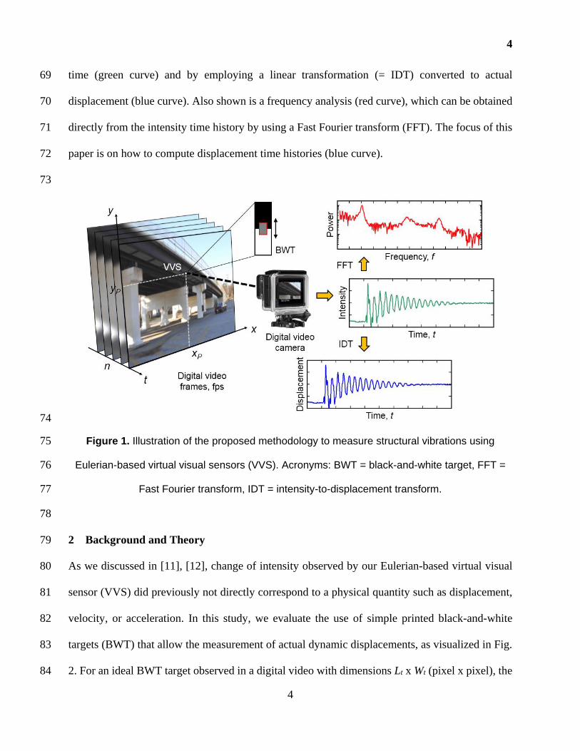
between the member and the background exists. Fig. 1 illustrates the concept of our proposed 66

methodology: a BWT target is attached to a location of interest. From the digital video extracted 67

from the camera, a VVS located on the BWT is selected. The change of intensity is recorded over 68

4

4

time (green curve) and by employing a linear transformation (= IDT) converted to actual 69

displacement (blue curve). Also shown is a frequency analysis (red curve), which can be obtained 70

directly from the intensity time history by using a Fast Fourier transform (FFT). The focus of this 71

paper is on how to compute displacement time histories (blue curve). 72

73

74

Figure 1. Illustration of the proposed methodology to measure structural vibrations using 75

Eulerian-based virtual visual sensors (VVS). Acronyms: BWT = black-and-white target, FFT = 76

Fast Fourier transform, IDT = intensity-to-displacement transform. 77

78

2 Background and Theory 79

As we discussed in [11], [12], change of intensity observed by our Eulerian-based virtual visual 80

sensor (VVS) did previously not directly correspond to a physical quantity such as displacement, 81

velocity, or acceleration. In this study, we evaluate the use of simple printed black-and-white 82

targets (BWT) that allow the measurement of actual dynamic displacements, as visualized in Fig. 83

2. For an ideal BWT target observed in a digital video with dimensions Lt x Wt (pixel x pixel), the 84

5

5

pattern colors are represented by the minimum and maximum intensity values (Imin. and Imax., 85

respectively) corresponding to 0 (= black) and 255 (= white), respectively. The displacement varies 86

linearly with VVS patch intensity, Ip(t): 87

88

max min

p p

p

I II t x t n t

L

(1) 89

90

where Ip(t) is the average pixel intensity across the patch area, Ap = Wp x Lp (pixel x pixel) for a 91

frame at time instant, t (sec), x(t) (pixel) measured displacement, and Lp (pixel) is the length of the 92

patch. It is assumed that intensity across the width of the patch, Wp (pixel) is constant and it 93

therefore does not appear in Eq. (1). It should be noted that the patch length, Lp (pixel) should be 94

large enough to account for the maximum displacement amplitude, A (pixel), i.e. Lp > A. At the 95

same time, the length of the target, Lt (pixel) needs to be able to accommodate for the patch length, 96

Lp (pixel), i.e. the target cannot leave the patch, otherwise the relationship becomes non-linear. 97

Finally, there is no perfect BWT target (with perfect black (I = 0) or white (I = 255) intensity 98

values) in a real setting and measurement noise is always present. The total average noise of the 99

patch, np(t) can be defined as: 100

101

1

1 N

p i

i

n t n tN

(2) 102

103

where N is the total number of pixels in the VVS patch and ni is the noise present in pixel i. 104

105

6

6

106

Figure 2. Illustration of the VVS measurement process using a black-and-white target (BWT): 107

the target, which is attached to the vibrating structural element, moves in the x-direction relative 108

to a fixed patch of pixels, i.e. having Eulerian-coordinates, as a function of time, t. 109

110

As an alternative to Eq. (1), VVS patch intensity, Ip(t) can also be computed as the average 111

intensity value of all pixels across the patch area, Ap: 112

113

1

1 N

p i

i

I t I tN

(3) 114

115

where N is the total number of pixels in the VVS patch and Ii is the intensity value of pixel i. 116

117

7

7

118

Figure 3. Illustration for the case where the camera is not oriented perpendicular to the 119

displacement component of interest, uact. O denotes the camera location and T the center 120

location of the target mounted to the vibrating structure. a and b represent horizontal and 121

vertical distance between the camera and the center of the target. 122

123

In order to correlate the observed intensity values to actual displacement, a calibration constant, 124

B (mm/pixel) needs to be determined. This is done by dividing the actual length of the BWT (mm) 125

by the corresponding number of pixels (pixels) observed from a selected frame of the video. For 126

the case where the camera is not oriented perpendicular to the displacement component of interest, 127

i.e. when b ≠ 0, a geometric correction factor, C (unitless) applies. This factor is calculated based 128

on the location of the camera (O) and the center location of the target (T), as illustrated in Fig. 3: 129

130

1

1

cos tan

Cb

a

(4) 131

132

Motion observed at angles ≠ 90 Degrees about the axis aligned with that motion (in our case 133

vertical) are not affected in any significant manner and are thus not considered. 134

8

8

Considering that Ip(t) is known and by using the calibration constant, B (mm/pixel) and the 135

geometric correction factor, C, the actual dynamic displacement of the target, uact(t) can be 136

computed using the following relationship: 137

138

act pu t B C I t (mm) (5) 139

140

Changing lighting conditions affect the measured intensity values and thus introduce an error in 141

the prediction of uact(t). This is really only a problem for long-term measurements (e.g. for SHM 142

applications) but can be addressed by continuously normalizing the difference of the measured 143

intensity values on the target (Imax – Imin) when lighting conditions change. For short-term 144

measurements (e.g. annual impact or load tests) where the test time can be selected accordingly, 145

this effect is negligible. 146

147

The presence of noise may require implementation of a noise reduction technique. Fortunately, 148

for a BWT the averaging process (expressed by Eqs. (1) and (3)) by itself helps reducing the noise, 149

i.e. the power of the noise reduces directly with the number of pixels in the patch, N. Assuming 150

that the noise is independent of the signal and can be represented by a stationary process, we arrive 151

at: 152

153

2 2

max min2 2

2

p

p

p

nI II x

L N

(6) 154

155

9

9

Eq. (6) relates the size of the VVS patch and the power of the noise and the signal. As can be 156

seen from the second term of the right hand side of Eq. (6), as the number of pixels increases the 157

power of the noise decreases. However, increasing the length of the patch will have the same effect 158

on the power of the signal, hence keeping the length as short as possible and the width as large as 159

possible will maximize the SNR. Substituting N for WpLp in Eq. (6), which is width x length of the 160

patch, we can get the following expression for the signal-to-noise ratio (SNR): 161

162

2

2max min

2 22

max min2 2

p p

pp p

p p

I Ix

L W xSNR I I

Ln n

W L

(7) 163

164

Eq. (7) shows that in order to reach the maximum SNR one has to maximize the Wp-to-Lp ratio 165

keeping in mind that Lp should be able to cover the maximum displacement amplitude, A, as 166

discussed earlier. For a specific camera and lighting conditions, the pixel noise power can be 167

assumed constant and the appropriate size of the patch can be specified based on the desired SNR. 168

The other factor that should be discussed in Eq. (7) is the second factor, max minI I , which has a 169

more significant effect on the SNR. It can be concluded from Eq. (7) that the higher the contrast 170

between black and white in the target, the higher the SNR will be. 171

172

3 Experiments 173

3.1 Laboratory Setup and Instrumentation 174

A laboratory-scale three-degree-of-freedom structural system (Total height = 610 mm (2 ft) as 175

shown in Fig. 4 (d) was used to evaluate the accuracy of the methodology proposed in Section 2. 176

10

10

The structure was excited by introducing random initial displacements at two locations on the 177

structure by hand followed by a sudden release to initiate free vibration. A digital camera (GoPro 178

Hero 3, shown in Fig. 4 (c))) capturing the free vibration response was located 305 mm (1 ft) away 179

from the structure. The displacement of the first floor was also measured using a 12.7 mm (0.5 in) 180

amplitude potentiometer (Fig. 4 (b)) connected to a high-speed data acquisition system (Fig. 4 (a)) 181

using a sampling frequency of 1200 Hz. The frame rate of the digital camera was 60 frames per 182

seconds (fps). 183

184

185

Figure 4. Experimental setup: (a) high-speed data acquisition system, (b) potentiometer to 186

measure displacements at the first story mass, (c) digital camera to collect VVS data, and (d) 187

three-degree-of-freedom laboratory structure. 188

189

3.2 Data Acquisition and Data Preprocessing 190

11

11

In order to compare the two measured signals, two steps have to be taken: (1) synchronization of 191

the signals in the time domain and (2) multiplication of the measured signals by their appropriate 192

calibration factors to obtain actual displacement from the measured data. It is good to mention that 193

the max minI I value was assumed to be constant, which proved to be a correct assumption based 194

on the data. Also the calculation of this value was based on the average of a black and white patch 195

of pixels on the target that was taken from a snapshot of the videos. For step (1), both camera and 196

potentiometer data were interpolated linearly to two equivalent 3000 Hz signals. Based on the 197

maximum correlation between the two signals, the time lag between the two signals was calculated 198

and one of the signals shifted so that they had a common time axis. In order to achieve actual 199

displacement for step (2), the potentiometer was calibrated against a precision height gage. The 200

mean calibration factor was found to be 1.257 mm/V (0.0495 in/V). For the camera intensity data, 201

the known target length, Lt was measured in a video frame in terms of pixels, which produced a 202

mean calibration factor of 0.279 mm/pixel (0.011 in/pixel). 203

204

In addition to the independent application of calibration factors as described above, it was also 205

possible to multiply the VVS intensity data by a factor that minimizes the second norm of 206

difference, or error, between the two measurements. This case represents the optimal estimate of 207

the displacement for the VVS, assuming the potentiometer represents an accurate reference 208

measurement. Obviously, in a real life scenario only the first approach can be used where a 209

calibration factor has to be estimated from the video data. It should be noted that the potentiometer 210

serves as the reference measurement but does not necessarily produce a more accurate 211

displacement. This was particularly visible at the peak displacement points and is discussed in 212

more detail in Section 4.1. 213

12

12

214

4 Results 215

4.1 Accuracy of Proposed Approach 216

Two VVS patch sizes, Wp x Lp = 40 x 50 and 40 x 100 pixels, were selected to study how the 217

accuracy of the measurements change with the size of the VVS patch, Ap. Fig. 5 shows a snapshot 218

of a video frame with the target and the two evaluated VVS patch sizes. 219

220

221

Figure 5. Photo of BWT target with two VVS patch sizes: (a) 40 x 50 pixel patch and (b) 40 x 222

100 pixel patch. 223

224

Fig. 6 shows a comparison of a sample measurement using independent calibration factors, as 225

described in Section 3.2. As can be observed from Fig. 6 (a), the displacements measured by the 226

VVS and the potentiometer are, qualitatively, in close agreement for both patch sizes. However, 227

the inserts in Fig. 6 (a) reveal that the end of the signal of the 40 x 100-pixel patch resembles the 228

potentiometer’s measurement more closely. A direct correlation between the two measurements 229

(Fig. 6 (b)) shows approximately a straight line with a slope of 0.95 and 0.92 with a squared 230

correlation coefficient of 99.6 and 99.9% for the patch size of 40 x 50 and 40 x 100 pixels, 231

respectively. The absolute prediction error at the 95% confidence level was determined by 232

13

13

measuring the distance between the 95% prediction limits shown in Fig. 6 (b) (red dotted lines) 233

and found to be 0.12 and 0.24 mm (0.0047 and 0.0094 in) for the patch size of 40 x 50 and 40 x 234

100 pixels, respectively. Furthermore, in Fig. 6 (c), which shows the absolute value of the 235

difference between the two measurements, less than 2% of the signal difference is greater than a 236

pixel size and roughly 90% of the time the difference is less than half of a pixel size. It can further 237

be observed that the difference shows distinct evenly-spaced peaks that are highest at the beginning 238

of the signal. Also, they appear to coincide with the peak amplitudes of the signal. The difference 239

is likely due to an error in the potentiometer measurement, when the direction of the displacement 240

changes. Unfortunately, it was not possible for us to ascertain this claim completely. In the future, 241

we plan to perform further laboratory tests using a laser vibrometer. Despite this uncertainty, our 242

data shows that subpixel-level accuracy is achievable with high confidence. The actual difference 243

in terms of noise can be observed by visually comparing the curves in Fig. 6 (c) between 4 and 6 244

s. The distribution of the error with mean, and standard deviation, is shown in Fig. 6 (d). It can 245

be observed from the distribution of the signal difference that it appears to follow a Normal 246

distribution, as assumed in Section 2. 247

14

14

248

Figure 6. Comparison of results using independent calibration factors, 40 x 50 pixels (left 249

column) and 40 x 100 pixels (right column): (a) Time history signals of VVS patch data and 250

potentiometer, (b) correlation between the two measurements with regression lines, (c) absolute 251

value of the difference between the two signals (errors), and (d) histogram of the errors. 252

253

15

15

Fig. 7 shows the case where the calibration factor for the VVS was optimized as discussed in 254

Section 3.2. Fig. 7 (a) compares with Fig. 6 (a) while correlation plots shown in Fig. 7 (b) are even 255

better compared to Fig. 6 (b). The slope of the prediction line in Fig. 6 (b) is 0.99 and 0.98 with a 256

squared correlation coefficient of 99.5 and 99.9% for the patch size of 40 x 50 and 40 x 100 pixels, 257

respectively. The absolute prediction error at the 95% confidence level, computed as described 258

earlier, was found to be 0.26 and 0.11 mm (0.01 and 0.0043 in) for the patch size of 40 x 50 and 259

40 x 100 pixels, respectively. The maximum signal difference (Fig. 7 (c)) is reduced by almost 260

half of a pixel size as compared to Fig. 6 (c). Comparing the patch sizes in Fig. 7 (d), it can be 261

observed that the standard deviation of the pixel error has been significantly decreased from 0.23 262

pixels to 0.12 pixels for the 40 x 50-pixel patch compared to the 40 x 100-pixel patch, respectively. 263

Also, with a confidence of more than 90%, the error in the smaller patch is less than one third of a 264

pixel size while in the bigger patch it is less than one fifth of a pixel size. Again, this approach 265

represents the case where the calibration factor for the VVS sensor was optimized by minimizing 266

the difference between the two measurements. 267

In conclusion from Figs. 6 and 7, we have demonstrated that subpixel accuracy can be achieved 268

with high confidence, even without implementing a computationally-expensive block matching 269

algorithm, and that estimates of the dynamic displacement can be achieved in a laboratory setting 270

with absolute prediction errors of approximately 0.25 mm (0.01 in). 271

272

16

16

273

Figure 7. Comparison of results using calibration factors based on minimized difference 274

between measurements, 40 x 50 pixels (left column) and 40 x 100 pixels (right column): (a) 275

Time history signals of camera and potentiometer, (b) correlation between the two 276

measurements with regression lines, (c) absolute value of the difference between the two 277

signals (error), and (d) histogram of the error. 278

17

17

279

Table 1 summarizes the main results of the accuracy evaluation presented in this section. It can 280

be seen that the larger VVS patch (40 x 100 pixels) was closer to the potentiometer reading 281

compared to the smaller patch (40 x 50 pixels). For the displacements computed using the 282

independent factors, the larger sized VVS patch was closer to the potentiometer measurement. 283

However, the standard deviation of the difference for the larger patch remained the same because 284

of the calibration issues explained earlier. While this type of comparison can likely not be 285

performed in the field, as it would require an independent physical measurement of the 286

displacement, it allowed us to isolate and study the calibration errors and the inherent irreducible 287

noise using the proposed VVS. 288

289

4.2 Relationship of Noise and Patch Size 290

Fig. 8 (d) shows the relationship between patch noise and number of pixels in a VVS patch as 291

defined theoretically by Eq. (7) and observed experimentally. As can be seen in Fig. 8 (a), the 292

power of the noise is close to the theoretical values. Figs. 8 (b) and (c) show the distribution of the 293

noise for one pixel and a patch of 10 x 10 pixels. As can be observed, the noise in the patch follows 294

a Normal distribution and its power is one order of magnitude smaller than that for one pixel. Also, 295

the SNR values approximately change linearly with the width to length ratio of the patch as 296

predicted from Eq. (7). This validates the theoretical framework presented in Section 2. 297

298

18

18

299

Figure 8. Noise power and the signal-to-noise ratio (SNR): (a) Power of the noise vs. the 300

number of pixels in the VVS patch (N), (b) histogram of noise in one pixel, (c) histogram of noise 301

in a 10 x 10-pixel patch, and (d) the SNR values vs. width over length of the patch. 302

303

4.3 Dynamic In-Service Load Test on the Streicker Bridge 304

In order to evaluate the applicability of the proposed methodology in a real-world scenario, the 305

Streicker Bridge was tested dynamically with a black-white target (BWT) to compute 306

displacement. Located on the Princeton University campus, the bridge has a unique design with a 307

straight main deck section supported by a steel truss system underneath and four curved ramps 308

leading up to the straight sections, as shown in Fig. 9. One of the ramps was instrumented with a 309

fiber-optic measurement system during construction by Br. Branko Glisic from Princeton 310

University [14]. For our test, we installed an off-the-shelf Canon EOS Rebel T4i camera with a 311

19

19

standard Canon EF 75-30mm zoom lens aimed at one of the ramps, to take a 60 fps video while a 312

number of volunteers jumped up and down on it. A VVS patch having 60 x 20 pixels was chosen 313

to compute displacements. As can be seen in Fig. 8, the VVS is located at a black-and-white edge 314

on a target mounted to the edge of the bridge slab. This target was set up by Dr. Maria Feng’s 315

research team from Columbia University, who collected data for evaluation of their own video-316

based monitoring methodology [15]. The relationships in Eqs. (1) and (5) were used to compute 317

the actual vertical dynamic displacement from the collected VVS patch. The calibration constant, 318

B was estimated from the target size as 17.3 (mm/pixel); the geometric correction factor, C 319

estimated to be 1.02. 320

321

20

20

322

Figure 9. Photograph of the Streicker Bridge showing the measurement setup and the location 323

of the VVS. The insert shows the location of the 60 x 20 pixel VVS patch (red rectangular). The 324

target was installed by Dr. Maria Feng’s research team from Columbia University [15]. 325

326

The computed vertical displacement response of the ramp section due to the described dynamic 327

forcing for a duration of 15 seconds is presented in Fig. 10. In our earlier paper we already reported 328

that the natural frequencies for this same test were found to be the same as those measured by the 329

fiber-optic measurement system [14]. Although we have no other physical measurement available 330

to directly compare and verify our computed displacement, it is comparable in amplitude to what 331

21

21

the Columbia University team reported [15]. Also, the frequency peak is exactly the same as 332

reported by the same group. 333

334

335

Figure 10. Results from the dynamic load test on the Streicker Bridge: (a) Computed actual 336

vertical displacement time history and (b) frequency response of signal (a). 337

338

5 Discussion and Conclusions 339

The objective of this study was to evaluate the possibility of computing actual dynamic 340

displacements using Eulerian-based virtual visual sensors (VVS) . This is based on the idea that 341

either an edge of a vibrating structural element or a black-and-white target (BWT) can be 342

monitored by a patch of pixels. The noise in the VVS sensor was found to be inversely related to 343

the patch size. The following conclusions can be made from on our study: 344

22

22

The use of BWT allows for accurate computation of dynamic displacements of a vibrating 345

structural element comparable to the measurements from a potentiometer. 346

The laboratory tests demonstrated that sub-pixel accuracy can be achieved similar to block 347

matching algorithms. The absolute prediction error at the 95% confidence limit was found to 348

be approximately 0.25 mm (0.01 in) relative to the reference measurement. 349

The accuracy in the measurement of the displacement implies that change of intensity is highly 350

sensitive to even tiny amounts of movement, which results in the fact that natural frequencies 351

can be measured as proposed in [11]–[13] even if the displacement is much less than a pixel 352

size. 353

Our proposed approach also works in the field, as demonstrated by the measurements of the 354

Streicker Bridge. A direct validation was not possible since no other physical displacement 355

data was available, which is typically the case for field measurements. However, the frequency 356

content of the signal has already been verified in [18] and the displacement amplitude as well 357

as the frequency peak is comparable to what the team from Columbia University found [15]. 358

The influence of camera movement and changes in lighting conditions need to be addressed 359

further in future research. 360

361

Acknowledgments 362

The support by a Center for Advanced Infrastructure and Transportation University Transportation 363

Research (CAIT-UTC) grant (Contract No. DTRT12-G-UTC16) and the Department of Civil and 364

Environmental Engineering at the University of Delaware for this study is greatly appreciated. We 365

further thank our colleague Prof. Branko Glisic, who facilitated access for the field test on the 366

Streicker Bridge located on Princeton University’s campus. Finally, we would like to thank Dr. 367

23

23

Nakul Ramanna for assisting with the field test, Dr. Maria Feng and her team from Columbia 368

University for allowing us to use their target, and Mr. Marcus Schwing for his expertise in photo 369

editing. 370

371

References 372

[1] A. Deraemaeker and K. Worden, New trends in vibration based structural health 373

monitoring. 2012. 374

[2] S. W. S. Doebling, C. R. C. Farrar, M. B. M. Prime, and D. W. D. Shevitz, “Damage 375

identification and health monitoring of structural and mechanical systems from changes in 376

their vibration characteristics: a literature review,” 1996. 377

[3] C. R. Farrar and K. Worden, “An introduction to structural health monitoring.,” Philos. 378

Trans. A. Math. Phys. Eng. Sci., vol. 365, no. 1851, pp. 303–315, 2007. 379

[4] H. H. Nassif, M. Gindy, and J. Davis, “Comparison of laser Doppler vibrometer with contact 380

sensors for monitoring bridge deflection and vibration,” NDT E Int., vol. 38, no. 3, pp. 213–381

218, Apr. 2005. 382

[5] B. D. Lucas and T. Kanade, “An Iterative Image Registration Technique with an 383

Application to Stereo Vision,” IJCAI, vol. 130, pp. 674–679, 1981. 384

[6] H. Leclerc, J. Périé, S. Roux, and F. Hild, “Integrated digital image correlation for the 385

identification of mechanical properties,” Comput. Vision/Computer Graph. …, pp. 161–386

171, 2009. 387

[7] R. C. Oats, D. K. Harris, T. (Tess) M. Ahlborn, and H. A. de Melo e Silva, “Evaluation of 388

the Digital Image Correlation Method as a Structural Damage Assessment and Management 389

Tool,” in Transportation Research Board 92nd Annual Meeting, 2013. 390

24

24

[8] I. B. Mohammad Bolhassani, Satish Rajaram, Ahmad A. Hamid, Antonios Kontsos, 391

“Damage detection of concrete masonry structures by enhancing deformation measurement 392

using DIC,” in Nondestructive Characterization and Monitoring of Advanced Materials, 393

Aerospace, and Civil Infrastructure X, SPIE, 2016. 394

[9] C. A. Murray, W. A. Take, and N. A. Hoult, “Measurement of vertical and longitudinal rail 395

displacements using digital image correlation,” Can. Geotech. J., vol. 52, no. 2, pp. 141–396

155, Feb. 2015. 397

[10] Y.-Z. Song, C. R. Bowen, A. H. Kim, A. Nassehi, J. Padget, and N. Gathercole, “Virtual 398

visual sensors and their application in structural health monitoring,” Struct. Heal. Monit., 399

vol. 13, no. 3, pp. 251–264, Feb. 2014. 400

[11] T. Schumacher and A. Shariati, “Monitoring of structures and mechanical systems using 401

virtual visual sensors for video analysis: fundamental concept and proof of feasibility.,” 402

Sensors (Basel)., vol. 13, no. 12, pp. 16551–64, Jan. 2013. 403

[12] A. Shariati, T. Schumacher, and N. Ramanna, “Eulerian-based virtual visual sensors to 404

detect natural frequencies of structures,” J. Civ. Struct. Heal. Monit., vol. 5, no. 4, pp. 457– 405

468, 2015. 406

[13] A. Shariati and T. Schumacher, “Oversampling in virtual visual sensors as a means to 407

recover higher modes of vibration,” in AIP Conference Proceedings (Proceedings of QNDE 408

2014, July 20-25, Boise, ID.), no. Dic, pp. 1–7. 409

[14] B. Glisic, J. Chen, and D. Hubbell, “Streicker Bridge: a comparison between Bragg-grating 410

long-gauge strain and temperature sensors and Brillouin scattering-based distributed strain 411

and temperature sensors,” in SPIE Smart Structures and Materials + Nondestructive 412

Evaluation and Health Monitoring, 2011, p. 79812C–79812C–10. 413

25

25

[15] D. Feng, M. Q. Feng, E. Ozer, and Y. Fukuda, “A Vision-Based Sensor for Noncontact 414

Structural Displacement Measurement.,” Sensors (Basel)., vol. 15, no. 7, pp. 16557–75, Jan. 415

2015. 416

417

418

26

26

Table1. Summary table of accuracy evaluation. 419

Independent calibration

factors

(see Fig. 6)

Minimization of signal

difference

(see Fig. 7)

Size of the patch 40 x 50 40 x 100 40 x 50 40 x 100

Correlation Coefficient 0.998 1.000 0.998 1.000

Maximum difference in pixel size 1.5 1.2 1.5 0.6

Mean of the difference 0.105 0.007 0.018 -0.014

Standard deviation of the difference 0.277 0.300 0.236 0.124

420