IMAGE GUIDED TRANSORBITAL ENDOSCOPIC PROCEDURES

By

Nkiruka Atuegwu

Dissertation

Submitted to the Faculty of the

Graduate School of Vanderbilt University

In partial fulfillment of the requirements

For the degree of

DOCTOR OF PHILOSOPHY

In

Biomedical engineering

December 2008

Nashville, Tennessee

Approved:

Robert L. Galloway

Michael I. Miga

Louise A. Mawn

Alfred. B. Bonds

Jay. B. West

iii

ACKNOWLEDGEMENTS

First of all, I will like to thank my advisor and mentor Dr Bob Galloway for his support,

guidance and encouragement. This work and my PhD career will not have been possible without

him.

I will like to thank my other committee members Dr Louise Mawn, Dr Michael Miga, Dr

Jay West and Dr Alfred Bonds for all their help and advice throughout these years. I appreciate

all the time, effort and input that all they have given me over the course of my research.

I will like to thank Dr Cari Lyle and Dr Lillian Ringsdorf for their help with data

collection. I will also like to thank the Vanderbilt CT staff for all their help with image

acquisition.

This work will not have been possible without the various members of the SNARL and

BML lab (past and present). Thank you all for your input, assistance and friendship throughout

these years.

To my friends and family, I appreciate all the love, support and encouragement you have

given me and to my husband Emeka, I cannot thank you enough for always being there for me.

iv

TABLE OF CONTENTS

Page

ACKNOWLEDGEMENTS .......................................................................................................... III

TABLE OF CONTENTS .............................................................................................................. IV

LIST OF TABLES ........................................................................................................................ VI

LIST OF FIGURES ..................................................................................................................... VII

CHAPTER

I. PURPOSE AND SPECIFIC AIMS ...................................................................................... 1

II. BACKGROUND .................................................................................................................. 3

Endoscopy ................................................................................................................................... 3

Orbital Endoscopic Procedures ................................................................................................... 5

Image Guided Surgery and Interventions.................................................................................. 12

Registration ........................................................................................................................... 13

Localization and Tracking ..................................................................................................... 14

Magnetic Tracker: Aurora..................................................................................................... 15

Motivation for the specific aims................................................................................................ 19

References ................................................................................................................................. 20

III. MANUSCRIPT 1- VOLUMETRIC CHARACTERIZATION OF THE AURORA

MAGNETIC TRACKER SYSTEM FOR IMAGE GUIDED TRANSORBITAL ENDOSCOPIC

PROCEDURES............................................................................................................................. 22

Abstract ..................................................................................................................................... 22

Introduction ............................................................................................................................... 23

Materials and methods .............................................................................................................. 28

Results ....................................................................................................................................... 38

Discussion ................................................................................................................................. 45

References ................................................................................................................................. 47

IV. MANUSCRIPT 2- SENSITIVITY ANALYSIS OF FIDUCIAL PLACEMENT ON

TRANSORBITAL TARGET REGISTRATION ERROR. .......................................................... 49

Abstract ..................................................................................................................................... 49

Introduction ............................................................................................................................... 50

Materials and Methods .............................................................................................................. 52

Results ....................................................................................................................................... 63

Discussion ................................................................................................................................. 71

v

References ................................................................................................................................. 72

V. MANUSCRIPT 3- IMAGE GUIDED TRANSORBITAL ENDOSCOPIC PROCEDURE

IN PHANTOMS ........................................................................................................................... 74

Abstract ..................................................................................................................................... 74

Introduction ............................................................................................................................... 75

Methods ..................................................................................................................................... 80

Results ....................................................................................................................................... 84

Discussion ................................................................................................................................. 89

Acknowledgement ..................................................................................................................... 89

References ................................................................................................................................. 90

VI. SUMMARY ...................................................................................................................... 92

APPENDIX

A. ACCURACY MEASUREMENT OF THE EFFECT OF SOME MATERIALS ON THE

AURORA MAGNETIC SYSTEM ............................................................................................... 94

B. DEALING WITH CORRELATED FLE .......................................................................... 96

vi

LIST OF TABLES

Table Page

Effects of different substances on retinal damage caused by optic nerve injury, NMDA-induced

toxicity or ischaemia [9] ............................................................................................................... 10

The minimum and the maximum variances obtained for fiducials 1 and 121 and the number of

points that correspond to the minimum and maximum values. Table also shows the variance

calculated with 150 points. ........................................................................................................... 33

Random FLE of both the 5D and the 6D sensors for a z value of 4cm ........................................ 42

Relative Spatial FLE of both the 5D and the 6D sensors for a z value of 4cm ............................ 42

Random FLE of both the 5D and the 6D sensors for a z value of 6cm ........................................ 43

Relative Spatial FLE of both the 5D and the 6D sensors for a z value of 6cm ............................ 43

Random FLE of both the 5D and the 6D sensors for a z value of 12cm ...................................... 44

Relative Spatial FLE of both the 5D and the 6D sensors for a z value of 12cm .......................... 44

The mean, standard deviation and the maximum values of the RMS distance of the localized

fiducial points from the mean of the distances. ............................................................................ 65

The accuracy and the time of image guided and non image guided endoscopic phantom studies 89

Errors and variances due to the different materials ...................................................................... 95

Translational TRE values for the optimized fiducial configuration ............................................. 99

Translational TRE values for the unoptimized fiducial configuration ......................................... 99

vii

LIST OF FIGURES

Figure Page

Picture of a flexible endoscope. [http://en.wikipedia.org/wiki/Endoscopy] ................................... 4

Schematic of the optic nerve within the retrobulbar space [http://www.wetcanvas.com] .............. 6

The Aurora magnetic tracker system from NDI[http://www.ndigital.com/] ................................ 16

Schematic of the metal and field source and sensor distance ....................................................... 18

Diagram of the Aurora magnetic tracker. A is the field generator and B is the sensor ................ 25

Schematic and setup of the grid used for the measurement. A shows grid measurements and B

shows the setup for the data collection. ........................................................................................ 30

Variance calculated for fiducial 1 and 121 using 50 to 1000 points. The asterisks represent

fiducial 1 and circles represent fiducial 121. ................................................................................ 32

Schematic of the volumetric movement of the measurement grid for the endoscopic procedure. 34

Schematic of the different possible positions of the Aurora system. The dark gray orbital region

shows the orbit of interest ............................................................................................................. 36

The schematic of the orbital triangle formed for position A in Figure 9. ..................................... 37

Graph of the random FLE of a sample plane (plane 2) intersecting the magnetic field. Figure on

the left is the 6D and the figure on the right is the 5D. ................................................................. 39

Figure showing the relative spatial error of a sample plane (plane 5) intersecting the magnetic

field. The figure on the left shows the error for the 6D and the figure on the right shows the error

for the 5D tracker. ......................................................................................................................... 40

Cartoon of the target region. The stars show the target region and some of the possible locations

of the target. .................................................................................................................................. 58

Picture of the face with the skin fiducials and the LADS with reference frame attached. ........... 61

viii

a) Skull phantom with the initial and final fiducial positions. The squares are the initial fiducial

position and the circles are the final fiducial position. b) Laser range scan of the skull phantom

with the taboo regions. .................................................................................................................. 64

TRE calculated in the target region for FLE value of 1mm for an initial naïve initial fiducial

position .......................................................................................................................................... 67

TRE calculated in the target region for FLE value of 4mm for an initial naïve initial fiducial

position. ......................................................................................................................................... 68

Average TRE in the target region for ten different simulations of the simulated annealing

program ......................................................................................................................................... 70

Picture of the possible placements of the magnetic tracker[13] ................................................... 79

Picture of the experimental setup .................................................................................................. 81

Screen shot of the ORION image guidance software used. The three planes show the three

orthogonal views of the skull phantom and the last plane shows the endoscopic view. .............. 83

Graph of the non image guided times vs. the image guided times for the different targets for the

attending surgeon. The line represents the times when the time to target with image guidance was

equal to the time to target with non image guidance. ................................................................... 85

Graph of the non image guided times vs. the image guided times for the different targets for the

surgical fellow. .............................................................................................................................. 87

Graph of the non image guided times vs. the image guided times for the different targets for the

surgical resident. ........................................................................................................................... 88

The possible placements of the Aurora magnetic tracker relative to the head. ............................ 97

Overlay of the skull phantom and the grid phantom ..................................................................... 98

Planar overlay of the grid phantom and skull phantom ................................................................ 98

1

CHAPTER I

PURPOSE AND SPECIFIC AIMS

Endoscopic orbital procedures are hindered by both the difficulty in differentiating

between orbital structures and the loss of orbital landmarks during these procedures. These

difficulties are due to the orbital fat that obstructs direct vision of the orbital structures. Image

guidance can address these problems because real time image and physical space tracking

information can be provided to the surgeons during the orbital procedure to help in the delivery

of therapy to the orbit.

The research plan proposes to study the feasibility of image guided endoscopic orbital

procedures. Specifically this research will:

Specific Aim 1: Characterize the magnetic tracking system.

The volumetric random and the spatially dependent fiducial localization error will be

characterized.

The accuracy of the sensor measurements in the presence of a flexible endoscope will

be characterized.

Specific Aim 2: Determining an optimal fiducial placement that minimizes TRE in a target

zone.

The optimal fiducial placement to minimize the TRE of the optic nerve eye junction

will be determined.

Sensitivity analysis will be performed on the fiducials to determine the effect of

random errors in fiducial placement on TRE.

2

Skin motion experiments will be carried out to give an estimate of the FLE due to

skin motion that can be expected.

Specific Aim 3: Validation of the possibility of image guidance to the optic nerve.

Image guided endoscopic orbital procedure will be compared to non image guided

endoscopic procedures using phantoms. The timing and targeting comparisons will be

used as a measure of the advantage and the possibility of image guided orbital

endoscopic procedures.

3

CHAPTER II

BACKGROUND

Endoscopy

Endoscopy is the examination and inspection of the interior of body organs, joints or

cavities through an endoscope inserted into the body through a natural or created aperture. It is a

minimally invasive procedure. An endoscope consists of a rigid or flexible tube and a light

delivery system to illuminate the organ or object under inspection. An endoscope uses two fiber

optic lines. A "light fiber" carries light into the body cavity and an "image fiber" carries the

image of the body cavity back to the physician's viewing lens. There is also a separate port to

allow for administration of drugs, suction, and irrigation. This port may also be used to introduce

small folding instruments such as forceps and scissors for tissue excision, sampling, or other

diagnostic and therapeutic work. Figure 1 is a picture of a flexible endoscope. Endoscopes can be

used for a variety of medical procedures such as bronchoscopy, gastroscopy and endoscopic

biopsy. Of importance to this work is the use of endoscopes for orbital procedures.

4

Figure 1: Picture of a flexible endoscope. [http://en.wikipedia.org/wiki/Endoscopy]

5

Orbital Endoscopic Procedures

The optic nerve’s location behind the globe in the intraconal space (Figure 2) makes open

surgical access available only to highly trained orbital surgeons. Access to the retrobulbar optic

nerve has traditionally required an orbitotomy; an invasive procedure in which either a rectus

muscle is dissected from the globe or the lateral boney wall of the orbit removed. It is not

practical to perform complex, invasive orbital surgery for the large numbers of individuals

suffering from optic nerve disease. The use of endoscopes can reduce this invasiveness.

Endoscopes were first used by Norris and Cleasby in the late 1970’s for orbital surgery

and later for orbital biopsies. They made an initial attempt at guidance with a stereotaxic

positioner to hold the endoscope at a fixed position but they had great difficulty with the

stereotaxic arm and discontinued use [1-3]. Since then various attempts at using the endoscope in

the orbit have been reported.

Recently, Mawn et all used a flexible endoscope to navigate the orbit for optic nerve

sheath fenestration (ONSF). They reported that there were problems with navigation through the

orbit because the orbital structures were of similar color and also because the traditional orbital

landmarks were lost as the endoscope was moved through the orbit. They also reported that it

took as much as 3 hours to complete an ONSF in a human cadaver [4].

6

Figure 2: Schematic of the optic nerve within the retrobulbar space [http://www.wetcanvas.com]

7

Potential Orbital Endoscopic Procedures

New research on neuroprotection has brought into the light other potential uses of

endoscope. Neuroprotection is the strategy of treating a disease by preventing neuronal death.

Neuroprotection is useful even when the exact cause of a disorder is undefined, as the therapy

occurs at the level of the dying cells and not at the initial site of injury.

Optic neuropathies, a group of diseases characterized by visual loss due to optic nerve

dysfunction are one of the main targets of neuroprotective therapy. The most common optic

neuropathy is that associated with glaucoma. Glaucoma in general results in changes in the

trabecular meshwork of the eye. Primary Open-Angle Glaucoma (POAG) and Primary Angle-

Closure Glaucoma (PACG) are characterized by damage to the optic nerve, retinal ganglion cell

death and visual field loss which include the loss of peripheral vision, depth perception, and

contrast sensitivity [5]. The optic nerve damage is thought to occur in the optic nerve head [6].

The number of people with primary glaucoma in the world in 2000 was estimated at nearly 66.8

million, with 6.7 million suffering from bilateral blindness [7]. It is estimated that there will be

60.5 million people with primary open-angle glaucoma (POAG) and primary angle-closure

glaucoma (PACG) in 2010, increasing to 79.6 million by 2020. Bilateral blindness

will be present

in 4.5 million people with POAG and 3.9 million people with PACG in 2010, rising to 5.9 and

5.3 million people in 2020, respectively [8].

A wide variety of other optic neuropathies also cause visual loss, e.g. inflammatory,

ischemic, infiltrative, and traumatic optic neuropathies. A number of factors can be responsible

for the disease, but in all types of optic neuropathy, the injury is manifested at the optic nerve

axon and results in the loss of retinal ganglion cells (RGCs) through apoptosis [9].

8

Several neuroprotective strategies may be useful for preventing retinal ganglion cell death after

axonal injury. These include delivery of neurotrophins, blockade of receptors mediating

excitotoxicity, and scavenging of reactive oxygen species [6].

9

Table 1 depicts pharmacological agents that affect the RGC cells that are damaged due to optic

nerve transection, NMDA- induced toxicity and ischemia. NMDA is an amino acid derivate that

acts as an agonist at an NMDA receptor.

While neuroprotective drugs are developed and tested, there is a need to effectively deliver the

drugs to the optic nerve especially to the axon [10].

10

Table 1: Effects of different substances on retinal damage caused by optic nerve injury, NMDA-

induced toxicity or ischaemia [9]

11

Current Methods of Ocular Drug Delivery

Topical administration of medications is the easiest method for drug delivery to the eye

but the disadvantage of this method is that topical delivery often fails to provide therapeutic

levels in the vitreous cavity or posterior segment because at least 80% of the applied medication

disappears via lacrimal drainage and does not enter the eye [11]. Other factors that hinder the

movement of the drug to the posterior regions include aqueous production, blood flow, and

barriers imposed by the corneal epithelium and endothelium and by the stromal tissues of the

cornea and sclera [12]. This makes topical administration of drugs an inadequate method for the

treatment of vitreoretinal diseases [13].

Transdermal therapeutic systems have been proposed for ocular drug delivery but they

only have a slight increase in concentration of the drug in the posterior segment when compared

to the topical drug delivery and, as such, are inadequate for treatment of posterior optical

neuropathies [12].

Drugs can often be delivered to the posterior segment by injection via the pars plana.

However, depending on the rate of clearance from the vitreous of a particular medication, large

boluses and frequent administrations may be required to ensure therapeutic

levels over an

extended period of time. Multiple intraocular injections can lead to an increased likelihood of

complications, such as vitreous hemorrhage, retinal detachment, and

endophthalmitis [13].

Intravitreal implants of sustained release drugs that provide constant levels of drug to the

eye have been used. The disadvantage of this is that drugs that are safe to the eye when used for a

short time may prove to be toxic when allowed to maintain long standing intraocular levels.

There are also risks associated with the surgical placement of intravitreal implants. These include

vitreous hemorrhage, retinal detachment, and

endophthalmitis [13]. Furthermore, not all the

12

drugs can be developed into an implant because an implant requires a coating material that does

not react to the drug and allows a sustained release of the drug. The feasibility of the use of the

intravitreal implants is limited in cases of trauma and damage to the vitreous of the eye where an

implant may not be feasible. In trauma cases, the need for immediate protection of RGCs before

additional surgery precludes the use of implants for immediate protection of the RGCs.

Most of the common methods of ocular drug deliveries do not effectively get the drugs to

the optic nerve axon and may have additional side effects. A system that can guide an endoscope

to the optic nerve for drug delivery can potentially be used for delivery of neuroprotective drugs

to the optic nerve cells.

For orbital endoscopic procedures to be used, the problem of navigation through the

orbital fat has to be improved since the orbital fat obscures easy visualization of optic nerve

during localization. This can be solved by the use of image guidance during the endoscopic

procedure.

Image Guided Surgery and Interventions

Image guided surgery and interventions involve the use of medical images to select, plan

and guide a surgical procedure or medical intervention. Because of the accuracy that image-

guided surgical technology provides, surgeons are able to create an exact, detailed plan for the

surgery and the intervention — where the best spot is to make the incision, the optimal path to

the targeted area, and what critical structures must be avoided. The real-time feedback provided

by the computer helps surgeons make adjustments to ensure they are exactly treating the desired

areas.

Image guided surgery is based upon integration of the preoperatively acquired and

processed information such as an image volume of the patient and the corresponding anatomy of

13

the patient within the same frame of reference. The images can be projective images such as

plane films and angiograms; tomographic sets such as computed tomography (CT), magnetic

resonance imaging, (MRI), single-photon emission computed tomography (SPECT), positron

emission tomography (PET) and Functional MRI (fMRI). It can also include intraoperative two-

dimensional imaging such as ultrasound images, laparoscopic, endoscopic and microscopic

images. Links between these two components are realized by combining image-to-patient

registration and by tracking instruments within the operating field.

Registration

Registration can be defined as the determination of a one to one mapping between the

coordinates in one space and those in another, such that the points in the two spaces that

correspond to the same anatomic structure are mapped together. Image-based registration can be

divided into extrinsic and intrinsic methods [14]. Intrinsic methods rely on patient-generated

image content. Extrinsic methods rely on artificial objects attached to the patient. These objects

are designed to be well visible and accurately detectable in all of the relevant modalities. The

point derived from the intrinsic or extrinsic object used for registration is called a fiducial point

and the extrinsic object which contains the fiducial point is called a fiducial marker.

Two basic types of fiducial markers are used in neurosurgical IGS: bone implantable

markers [15] and skin surface fiducials [16]. Bone implanted fiducials generally are more

invasive and cannot be used for procedures that are repetitively done on a patient. Skin fiducials

are not invasive and can be used frequently on a patient. Since skin moves over the bone, skin

fiducials are by nature, more mobile than bone implantable markers, and this may lead to an

increase in the localization error of the skin fiducials. This increase in localization error leads to

an increase in TRE during the IGS procedure.

14

The quality of fiducial-based registration may be judged by several types of registration

error computed after the registration. The three main measures of registration are Fiducial

localization Error (FLE), Fiducial Registration Error (FRE) and Target Registration Error (TRE).

FLE is the error in locating the position of a fiducial. FRE is the distance between corresponding

fiducial points after registration. TRE is the distance between the corresponding ―target‖ points

after registration. ―Target‖ in this case means points other than the fiducial points. [17].

Some of the factors that contribute to the FLE are the accuracy of localization of a

fiducial by the tracking system, the signal to noise ratio of the image, the imaging markers used

and image distortion [17].

TRE is affected by both the FLE of the system and the placement of fiducials[18].

22 2

2 21

1 1 K Ki

i j i ii jj

rTRE r FLE

N K

1

Number of fiducials

Spatial dimension; K=3

Distance between the centroid of the fiducials and the target

=Eigenvalues of the fiducial arrangement

i

N

K

r

From equation 1, it can be observed that minimizing the error due to the placement of the

fiducials can lead to a decrease in the TRE observed especially in the cases when the FLE cannot

be minimized further. After registration is carried out, the surgical or interventional instruments

have to be tracked within the operational field.

Localization and Tracking

Physical space localization methods are used to track the three-dimensional position of

surgical instruments, digitize points and surfaces on the anatomy, and provide links between

15

preoperative image studies and any available intraoperative data. Localizers used for image

guided procedures can be reduced to two classes of devices: geometric and triangulation.

Geometric localizers use angle, extension, and/or bend systems to sense the position of

the procedural device. In triangulation, an emitter or emitters broadcast energy, or a reflector or

reflectors return energy, to a series of detectors at known locations. This is used to calculate the

position and orientation of the emitter. Triangulation systems can be ultrasonic, optical or

magnetic [19].

Optical and ultrasonic trackers are line-of-sight devices; a free optical path between

sensor assembly and emitter is necessary in order to acquire data. This makes optical tracking

systems unsuitable for the tracking of flexible endoscopes or other instruments in the body;

optical trackers cannot be embedded in instruments that are completely inserted in the body:

because a line of sight has to be maintained between the markers and the optical localizer

system. Magnetic trackers, however, do not have a line of sight problem and can be used to track

instruments within the body. For this reason, we choose to use a magnetic tracking system to

perform the physical space localization in this work.

Magnetic Tracker: Aurora

The Aurora system (Northern Digital Inc, Waterloo, Ontario) is an alternating current

(AC) magnetic localizer system which emits AC magnetic fields at a maximum of 40 Hz. It

consists of a field generator (right hand side of Figure 3), a control unit (left hand side of Figure

3), and small coil sensors that can be embedded in catheters, endoscopes, and other instruments.

16

Figure 3: The Aurora magnetic tracker system from NDI[http://www.ndigital.com/]

17

The Aurora field generator unit contains coils that generate electromagnetic field. When a

tracked tool is placed inside the magnetic field, voltages are induced in the sensor coils that are

embedded in the tools. The induced voltage is then used to calculate the position and orientation

with five or six degrees of freedom (x, y, z translations and two or three orientations) of the

sensor coils. As the magnetic fields are of low field strength and can safely pass through human

tissue, location measurement of an object is possible without the line-of-sight constraints of an

optical spatial measurement system.

The disadvantage of magnetic localizers is that they induce eddy currents in nearby

conductive materials. These eddy currents induce secondary magnetic fields that change the

induced voltages measured by the sensors. This change in induced voltage leads to systematic

tracking errors. The Aurora system attempts to minimize these deviations through an iterative

algorithm for position and orientation calculation but some changes in induced voltage in the

sensors are still observed.

Several groups have studied the effect of metallic materials on the accuracy of a magnetic

tracker. In theory, the error in the calculated position due to a metal object r is predicted to be

[20, 21]

Where: trd is the distance between the field source (transmitter) and the sensor (receiver), tmd the

distance between the field source (transmitter) and the metal and mrd the distance between the

metal and the sensor (receiver).

2

18

Figure 4: Schematic of the metal and field source and sensor distance

19

From the above equation, it can be seen that the error in localizing a point decreases as

the metal-transmitter and metal-receiver distances are increased. This indicates that while metals

in the work volume lead to incorrect sensor readings, careful placement of the transmitter and the

sensor in relation to the metals in the environment can help r the amount of error in the measured

position of the sensor.

Motivation for the specific aims

Image guidance requires an image-space to physical-space registration and tracking in

physical-space with a localizer. To effectively use a magnetic localizer for transorbital guidance,

the error metrics must be characterized so that expected guidance errors can be determined.

Characterizing and understanding some of the tracking errors of the magnetic tracker will also

help determine the best use of the tracker; the positional placement and the expected errors in

any given location from the tracker. Working in the ―sweet spot‖ of the magnetic tracker will

help reduce the FLE experienced during the image guidance procedure.

After characterizing the magnetic tracker, the registration of the physical-space to image-

space needs to be addressed. Since the target in this research is the optic nerve, a structure which

can be anywhere in the retroorbital pyramid, a new form of fiducial placement is created. In this

method the retroorbital pyramid was sampled and a fiducial placement which minimized TRE

throughout the possible location of the optic nerve head was determined.

After characterizing the magnetic localizer and determining an optimal fiducial

placement for the task of optic nerve drug delivery, the performance of the system had to be

tested. An experimental protocol which allowed performance quantification in an application

mimicking manner was developed. Performance metrics from that protocol were gathered on a

number of surgeons.

20

References

1. Norris JL, C.G., An endoscope for ophthalmology. American Journal of Ophthalmology,

1978. 85(3): p. 420-2.

2. Norris JL, S.W., Bimanual endoscopic Orbital Biopsy. Ophtalmology, 1985. 92(1): p. 34-

38.

3. Norris JL, C.G., Endoscopic orbital surgery. American Journal of Ophthalmology, 1981.

91(2): p. 249-252.

4. Mawn, L.A.S., Jin-Hui ; Jordan, David R.; Joos, Karen M. , Development of an Orbital

Endoscope for Use with the Free Electron Laser. Ophthalmic Plastic & Reconstructive

Surgery, 2004. 20(2): p. 150-157.

5. Coleman, A.L., Glaucoma. The Lancet, 1999. 354(9192): p. 1803.

6. Levin, L.A., Direct and Indirect Approaches to Neuroprotective Therapy of

Glaucomatous Optic Neuropathy. Survey of Ophthalmology, 1999. 43(Supplement 1): p.

S98.

7. Quigley, H.A., Number of people with glaucoma worldwide. British Journal of

Ophthalmology, 1996. 80(5): p. 389.

8. Quigley, H.A. and A.T. Broman, The number of people with glaucoma worldwide in

2010 and 2020. Br J Ophthalmol, 2006. 90(3): p. 262-267.

9. N Osborne, G.C., C J Layton, J P M Wood, R J Casson and J Melena, Optic nerve and

neuroprotection strategies. Eye, 2004. 18: p. 1075-1084.

10. Jeffrey, G., How does an axon grow? Genes and Development, 2003. 17: p. 941-958.

11. Lux, A., et al., A comparative bioavailability study of three conventional eye drops versus

a single lyophilisate. Br J Ophthalmol, 2003. 87(4): p. 436-440.

12. Myles, M.E., D.M. Neumann, and J.M. Hill, Recent progress in ocular drug delivery for

posterior segment disease: Emphasis on transscleral iontophoresis. Advanced Drug

Delivery Reviews, 2005. 57(14): p. 2063.

13. Velez, G. and S.M. Whitcup, New developments in sustained release drug delivery for

the treatment of intraocular disease. Br J Ophthalmol, 1999. 83(11): p. 1225-1229.

14. Maintz, J.B.A. and M.A. Viergever, A survey of medical image registration. Medical

Image Analysis, 1998. 2(1): p. 1.

15. Maurer, C.R., Jr., et al., Registration of head volume images using implantable fiducial

markers. IEEE Trans Med Imaging, 1997. 16(4): p. 447–462.

21

16. Barnett, G.H., D.W. Miller, and J. Weisenberger, Frameless stereotaxy with scalp-

applied fiducial markers for brain biopsy procedures: experience in 218 cases. Journal of

Neurosurgery, 1999. 91(4): p. 569-576.

17. West, J.B., et al., Fiducial Point Placement and the Accuracy of Point-based, Rigid Body

Registration. Neurosurgery, 2001. 48(4): p. 810-817.

18. Fitzpatrick, J.M., J.B. West, and C.R. Maurer, Jr., Predicting error in rigid-body point-

based registration. Medical Imaging, IEEE Transactions on, 1998. 17(5): p. 694.

19. Galloway, R.L., The Process and Development of Image-guided Procedures. Annual

Review of Biomedical Engineering, 2001. 3(1): p. 83-108.

20. Hummel, J.B., et al., Design and application of an assessment protocol for

electromagnetic tracking systems. Medical Physics, 2005. 32(7): p. 2371-2379.

21. Mark A. Nixon, B.C.M., W. Richard Fright and N. Brent Price The Effect of Metals and

Interfering Fields on Electromagnetic Trackers. Presence, MIT Press, 1998. 7(2): p. 204-

218.

22

CHAPTER III

MANUSCRIPT 1- Volumetric characterization of the Aurora magnetic tracker system for

image guided transorbital endoscopic procedures

Atuegwu N.C and Galloway R.L

Original form of manuscript appears in Phys. Med. Biol. 53 (2008) 4355-4368.

Abstract

In some medical procedures, it is difficult or impossible to maintain a line of sight for a

guidance system. For such applications, people have begun to use electromagnetic trackers.

Before a localizer can be effectively used for an image-guided procedure, a characterization of

the localizer is required. The purpose of this work is to perform a volumetric characterization of

the fiducial localization error (FLE) in the working volume of the Aurora magnetic tracker by

sampling the magnetic field using a tomographic grid. Since the Aurora magnetic tracker will be

used for image-guided transorbital procedures we chose a working volume that was close to the

average size of the human head.

A Plexiglass grid phantom was constructed and used for the characterization of the

Aurora magnetic tracker. A volumetric map of the magnetic space was performed by moving the

flat Plexiglass phantom up in increments of 38.4 mm from 9.6 mm to 201.6 mm. The relative

spatial and the random FLE were then calculated. Since the target of our endoscopic guidance is

the orbital space behind the optic nerve, the maximum distance between the field generator and

the sensor was calculated depending on the placement of the field generator from the skull.

For the different field generator placements we found the average random FLE to be less

than 0.06 mm for the 6D probe and 0.2 mm for the 5D probe. We also observed an average

relative spatial FLE of less than 0.7 mm for the 6D probe and 1.3 mm for the 5D probe. We

23

observed that the error increased as the distance between the field generator and the sensor

increased. We also observed a minimum error occurring between 48 mm and 86 mm from the

base of the tracker.

Introduction

The use of electromagnetic trackers for image-guided procedures has increased in

popularity in recent years [1-3]. This can be attributed to newer generations of electromagnetic

trackers that show both an increased accuracy and have a reduced sensor size [4] making them

easier to embed in instruments. Optical trackers, which are the most commonly used localizers

for image guidance, are line of-sight devices requiring a free optical path between the sensor

assembly and the tracked tool. The need for a line of sight makes optical tracking systems

unsuitable for instruments that are completely inserted into the body. Magnetic trackers on the

other hand do not require a line of sight because magnetic fields can pass through the body. This

makes magnetic trackers suitable for tracking flexible medical instruments such as endoscopes.

Since our lab is working on image-guided transorbital endoscopic procedures we chose to use an

Aurora magnetic tracking system for the image-guided procedure. The Aurora system (Northern

Digital Inc, Waterloo, Ontario) is an alternating current (ac) magnetic localizer system which

emits ac magnetic fields. It consists of a field generator (A) and a small coil sensor that can be

embedded in catheters, needles and other instruments (B). This is shown in Figure 5. The Aurora

field generator unit contains coils that generate the electromagnetic field.

Sensor coils imbedded into the tracked tool are exposed to the produced electromagnetic

field and these sensors measure the induced voltage. The induced voltage is then used to

calculate the position and orientation of the sensor coils. The coils return the sensor position and

orientation with five (5D) or six degrees (6D) of freedom (x, y, z translations and two or three

24

orientations). A disadvantage of magnetic localizers is that they induce eddy currents in nearby

conductive materials. These eddy currents create an opposing magnetic field to the original

external magnetic field. The intersection of Aurora’s magnetic field with the opposing magnetic

field disrupts the magnetic field and can affect the transformation data produced. This leads to

systematic tracking errors.

Several groups have studied the effect of metallic materials on the accuracy of a magnetic

tracker [5-7]. From equation 1[6], the error in the reported position due to a metallic object r

is predicted to be

4

3 3

dr

d d

tr

tm mr

dtr is the distance between the field source (transmitter) and the sensor (receiver), dtm the

distance between the field source (transmitter) and the metal and dmr the distance between the

metal and the sensor (receiver). From equation 3, it can be observed that the error in localizing a

point decreases as the metal-transmitter and metal-receiver distances are increased. This

indicates that although metals in the working volume can lead to incorrect sensor readings,

careful placement of the transmitter and the sensor in relation to the metals in the environment

can help reduce the amount of error in the measured position of the sensor.

3

25

Figure 5: Diagram of the Aurora magnetic tracker. A is the field generator and B is the sensor

26

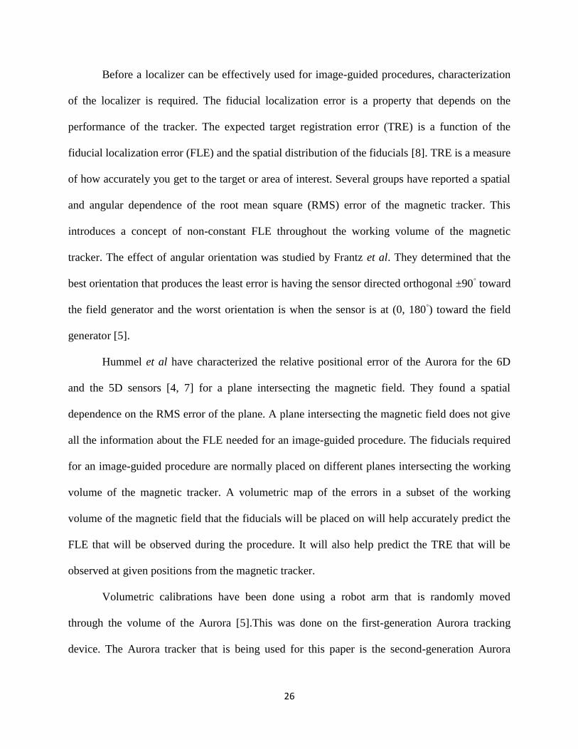
Before a localizer can be effectively used for image-guided procedures, characterization

of the localizer is required. The fiducial localization error is a property that depends on the

performance of the tracker. The expected target registration error (TRE) is a function of the

fiducial localization error (FLE) and the spatial distribution of the fiducials [8]. TRE is a measure

of how accurately you get to the target or area of interest. Several groups have reported a spatial

and angular dependence of the root mean square (RMS) error of the magnetic tracker. This

introduces a concept of non-constant FLE throughout the working volume of the magnetic

tracker. The effect of angular orientation was studied by Frantz et al. They determined that the

best orientation that produces the least error is having the sensor directed orthogonal ±90◦ toward

the field generator and the worst orientation is when the sensor is at (0, 180◦) toward the field

generator [5].

Hummel et al have characterized the relative positional error of the Aurora for the 6D

and the 5D sensors [4, 7] for a plane intersecting the magnetic field. They found a spatial

dependence on the RMS error of the plane. A plane intersecting the magnetic field does not give

all the information about the FLE needed for an image-guided procedure. The fiducials required

for an image-guided procedure are normally placed on different planes intersecting the working

volume of the magnetic tracker. A volumetric map of the errors in a subset of the working

volume of the magnetic field that the fiducials will be placed on will help accurately predict the

FLE that will be observed during the procedure. It will also help predict the TRE that will be

observed at given positions from the magnetic tracker.

Volumetric calibrations have been done using a robot arm that is randomly moved

through the volume of the Aurora [5].This was done on the first-generation Aurora tracking

device. The Aurora tracker that is being used for this paper is the second-generation Aurora

27

tracker. There has been a considerable increase in the accuracy of the system from the first-

generation to the second-generation system [4]. The results were also reported as a function of

the radial distance from the tracker. The radial distance calculation assumes a known center for

the magnetic field source in the field generator. Since the magnetic field source position is

unknown, a radial distance does not help in determining the FLE at certain distances from the

surface of the Aurora tracker. Also Wilson et al proposed a protocol for the evaluation of the

accuracy of the Aurora in a volume. This was done with a cubic phantom with holes drilled at

random positions throughout the volume. They obtained the average error in the working volume

of the Aurora with the field generator at different distances from the field generator and at

different environments [9]. We propose to get planar errors so that errors in each plane can be

evaluated separately. For purposes of image guidance, the FLE that can be expected at certain

distances in the three cardinal planes from the Aurora will be useful for the placement of the

Aurora magnetic tracker during the image-guided procedure. Planar results will help determine

the change in errors in the system with respect to the different cardinal planes of the Aurora. This

will help determine the error that will be expected at different distances from the Aurora field

generator.

The purpose of this work is to perform a volumetric characterization of the FLE in the

working volume of the Aurora magnetic tracker by sampling the magnetic field using a

tomographic grid. Since the Aurora magnetic tracker will be used for image-guided transorbital

procedures we chose a working volume that was close to the average size of the human head.

28

Materials and methods

To characterize the error in the magnetic tracker, a 22.6 cm by 22.6 cm square Plexiglass

grid phantom with 11 by 11 divots 0.8 inch (2.032 cm) apart as shown in Figure 6 was

constructed. The divots were 1 mm in radius drilled with a machine precision of 25 μm. The

dimensions of the phantom (22.6 cm2) were chosen to be close to the average size of a human

head. For the measurements we chose the tracker to be 7.4 cm away from the first divot. This

was chosen as a minimal convenient distance the magnetic field generator could be at for the

tracker to be used for image-guided transorbital guidance without the physician bumping into the

tracker during the procedure. Figure 8 shows a layout of the setup used for the data collection.

For our measurements we chose the sensor to be orthogonal to the field generator. The phantom

was designed to limit the variation in the angles of the sensors during data collection. We

acknowledge that they may be angular dependences in the measured error but that is beyond the

scope of this paper. Prior to the measurements, the plate and field generator were rigidly attached

to a wooden board.

FLE of the tracker

The FLE of the magnetic tracker can be modeled as sum of the random component of the

FLE and the spatial component of the FLE.

total random spatialFLE =FLE +FLE

The random component of the FLE is a result of the localization noise in the system. It is

the precision in localizing the same point using the magnetic tracking system.

random mechanics_of_tracker repositioningFLE = FLE +FLE

4

5

29

To remove the effect of the FLE due to the repositioning of the sensor during data

collection, one set of continuous time points were taken for each measurement. The random FLE

due to the mechanics of the tracker is the error due to the internal workings of the tracker. It

measures the error such as the stability of the coils that produce the magnetic fields and the

stability of the sensors and the position calculation algorithm. The random FLE due to the

mechanics of the localizer was calculated as the sum of the variance of the signal in the three

cardinal planes.

2 2 2 2random x y zFLE =σ +σ +σ

The spatial FLE is the accuracy of the localized point compared to the ―true‖ value of the

point. Since the ―true point‖ cannot be defined, the relative spatial FLE of the magnetic tracker

was calculated instead.

aurora_divotspatial absolute relative_spatialFLE = FLE + FLE

The relative spatial component of the FLE was calculated using the grid experimental

setup in figure 2. The absolute distance between the first rows of divots closest to the tracker is

subtracted from all the subsequent grid rows and this is compared to the actual machine precision

distance of the divots. This is done for the 3 cardinal plane positions to give a spatial error

distance map of the plane intersecting the magnetic tracker at sampled points.

_relative spatial aurora machineFLE Dist Dist

auroraDist is the distance between the rows of divots in Aurora space and machineDist is the machine

precision distance.

6

7

8

30

A

B

Figure 6: Schematic and setup of the grid used for the measurement. A shows grid measurements

and B shows the setup for the data collection.

31

To determine the number of data points to be collected for the FLE measurements, 1000

continuous points were collected for two divots (1 and 121). These divots corresponded to the

beginning of the grid and the last point of the grid. Different continuous time samples were used

to calculate the variance of the data in order to determine the change in the variance of the data

as a function of the number of sampled points used for the calculation. The first 50 points were

initially selected and this was increased incrementally by 50 points to 1000 points. Figure 7

shows the graph of the variance calculated with different number of time measurements. Table 2

also shows the maximum and minimum variance obtained using the different time points and the

variance obtained using 150 points. From Figure 7 and Table 2 , it can be observed that

deviations in the variance from the variance calculated with 150 points were not significant when

compared to the minimum variances measured between 50 and 1000 points. Therefore 150

points can accurately predict the variance of the time points and thus predict the FLE of the

system. So for the calculation of both the random and the relative spatial error of the magnetic

tracker, 150 points were used.

32

Figure 7: Variance calculated for fiducial 1 and 121 using 50 to 1000 points. The asterisks

represent fiducial 1 and circles represent fiducial 121.

33

Table 2: The minimum and the maximum variances obtained for fiducials 1 and 121 and the

number of points that correspond to the minimum and maximum values. Table also shows the

variance calculated with 150 points.

A volumetric map of the magnetic space forming a type of tomographic phantom was

performed by moving the flat Plexiglass phantom up in the x-axis in increments of 38.4 mm from

9.6 mm to 201.6 mm. The final stopping distance was chosen to correspond to the average size

of the human head. Figure 8 shows a schematic of the movement of the planes. For each plane, a

5D and a 6D sensor were used to localize each divot and the random and the relative spatial FLE

of each plane was calculated. The sensors used in each case were a 6D probe and a 5D flexible

catheter that were manufactured by Northern Digital Inc, Waterloo, Ontario.

Figure 9 is a schematic of the measurements of the orbit and the different possible positions of

the field generator for the image-guided transorbital procedure. Since the target of our

endoscopic guidance is the orbital space behind the optic nerve, the maximum distance between

the field generator and the sensor can be calculated depending on the placement of the field

generator from the skull.

34

Figure 8: Schematic of the volumetric movement of the measurement grid for the endoscopic

procedure.

35

As shown in Figure 9, positions A, B and C give some of the possible positions of the field

generator for the image-guided procedure. Ideally, position C will reduce the chances of the

tracker being bumped by the physician during the procedure.

Figure 10 shows a schematic of the orbital measurements in position A. From Figure 10,

if c = 4 cm, 0 < b _ 5 cm then a < 4 cm. Therefore the maximum z distance expected for position

A is 4 cm. For position B, the maximum z distance expected is 5 cm and for position C, the

maximum z distance expected is 10.5 cm. These distances were used to calculate the average

error that can be expected from the magnetic tracker if the field generator was kept at those

positions during the image-guided procedure. This was done by calculating the average error

from 0<z<maximum z. z = 0 corresponds to the starting point of the measurement with the

tracker 7.4 cm away from the sensor. Because of the setup of the grid, the nearest values that

were equal to or more than the calculated z values for positions A to C were chosen. We choose

A = 4 cm, B = 6 cm and C = 12 cm.

Effect of an endoscope on the accuracy of the magnetic tracker

Since the transorbital procedure is envisioned as an outpatient procedure that can be

performed in a procedure room, the metals in the environment can be accounted for. To find out

the effect of an endoscope on the flexible magnetic sensor, points were collected for a divot at a z

value of 6 cm. The divot was localized with only the 5D probe for a baseline measurement and

also localized with the sensor touching a flexible endoscope (Storz Flex X2, Karl Storz

Endoscopy America Inc). This was done ten different times and for each time the probe was

removed and the point was localized again. The mean of the 1500 points for the two different

measurements was calculated and this was used to calculate the effect of the endoscope on the

flexible 5D sensor.

36

Figure 9: Schematic of the different possible positions of the Aurora system. The dark gray

orbital region shows the orbit of interest

37

Figure 10: The schematic of the orbital triangle formed for position A in Figure 9.

38

Results

As expected the error increases in the z direction as the distance between the magnetic

sensor and the field generator increases. This increase was found in both the random FLE and the

relative spatial FLE of the tracker. Figure 11 shows a sample plane of the random FLE of both

the 5D and the 6D sensors. From the graph, it can be observed that the random FLE of the 5D

sensors fluctuates more than the random FLE of the 6D sensors.

The magnitude of the random error observed for the 6D sensor is smaller than that of the

5D sensor for each grid position and across the planes. The difference in the range of errors

observed can be attributed to the manufacture of the sensors. The 6D sensors have a redundancy

in them because they are made up of two 5D sensors that are at right angles to each other. This

reduces the error observed while using the 6D sensors. The average random error observed

across all the six planes and all the grid points for the 6D sensor is 0.093 ± 0.064 mm and the

average random error observed for the 5D sensor is 0.193 ± 0.10 mm.

The spatial error also increases as a function of the distance of the sensor from the field

generator. Figure 12 shows a sample plane of the relative spatial error of both the 5D and the 6D

sensors. On average, the relative spatial error for the 6D tracker is smaller than the relative

spatial error for the 5D tracker for all the grid points and across all the planes. The average

relative spatial FLE across the six planes and all the grid points for the 6D sensor was 1.35 ±

1.16 mm and the average relative spatial FLE for the 5D sensor was 2.34 ± 1.76 mm.

39

Figure 11: Graph of the random FLE of a sample plane (plane 2) intersecting the magnetic field.

Figure on the left is the 6D and the figure on the right is the 5D.

40

Figure 12: Figure showing the relative spatial error of a sample plane (plane 5) intersecting the

magnetic field. The figure on the left shows the error for the 6D and the figure on the right shows

the error for the 5D tracker.

41

The random FLE and the relative spatial FLE for the different field generator positions in

Figure 9 was calculated.

Tables 3 and 4 show the statistical values obtained for the random FLE and the relative

spatial FLE for the z = 4 cm (position A) for both the 5D and the 6D sensors. The magnitude of

the random and the relative spatial FLE for the 6D tracker is smaller than the magnitude of the

random and the relative spatial FLE for the 5D tracker for all the planes for position A. There is a

slight decrease in the average random and relative spatial FLE from plane 1 to plane 2 for both

the 5D and the 6D sensors. The errors increase from plane 2 to 3, which leads to a possibility of a

minimum occurring between plane 2 and plane 3 for the relative spatial FLE of both the 5D and

the 6D sensors. The average random and relative spatial FLE was calculated across all the six

planes. The average random FLE in all the six planes is 0.029 ± 0.014 mm for the 6D probe and

0.125 ± 0.063 mm for the 5D probe. The mean relative spatial FLE in all the six planes is 0.33 ±

0.22 mm for the 6D probe and 0.78 ± 0.37 mm for the 5D sensor.

Tables 5 and 6 show the statistical values obtained for z = 6 cm. The average random

FLE in all the six planes is 0.034 ± 0.017 mm for the 6D probe and 0.127 ± 0.063 mm for the 5D

probe. The same dip in the error described for z = 4 cm was observed for the FLE of the system

at z = 6 cm. The average spatial FLE for the six planes is 0.40 ± 0.27 mm for the 6D probe and

0.86 ± 0.42 mm for the 5D probe.

42

Table 3: Random FLE of both the 5D and the 6D sensors for a z value of 4cm

Table 4: Relative Spatial FLE of both the 5D and the 6D sensors for a z value of 4cm

43

Table 5: Random FLE of both the 5D and the 6D sensors for a z value of 6cm

Table 6: Relative Spatial FLE of both the 5D and the 6D sensors for a z value of 6cm

44

Table 7: Random FLE of both the 5D and the 6D sensors for a z value of 12cm

Table 8: Relative Spatial FLE of both the 5D and the 6D sensors for a z value of 12cm

45

Tables 7 and 8 show the statistical observation for each plane at z = 12 cm. The mean

random FLE for the 6D probe is 0.056 ± 0.037 mm and 0.152 ± 0.078 mm for the 5D probe. The

relative spatial FLE was 0.65 ± .44 mm for the 6D and 1.23 ± 0.67 mm for the 5D probe. The dip

in error observed for z = 4 and z = 6 cm was also observed in z = 12 cm.

Effect of the endoscope on the 5D sensor

The variance and the RMS error of the means of the 1500 points collected for the divot

with and without the endoscope were calculated. The variance of the divots without the

endoscope was 0.076 mm2 and the variance of the divot points with the endoscope was 0.081

mm2. This corresponds to a 0.0089 mm increase in the FLE of the sensor–endoscope

configuration versus the FLE of only the 5D sensor. The RMS error between the means of the

two divot points was 0.2 mm.

Discussion

In this paper, we characterized the fiducial localization error and the relative spatial errors

of a subset of the working volume of the Aurora tracker. This subset corresponds to the average

size of the human head. We observed that there was an increase in both the relative spatial FLE

and the random FLE of the tracker as the sensor moved further away from the tracker in the z

direction. We also observed that there was a dip in both the random and the relative spatial FLE

of the tracker as we sampled planar intersection of the working volume of the tracker. There was

a decrease in relative spatial error from plane 1 to 2. After plane 3 the error starts increasing from

the error in plane 2. Since the slice steps are fixed, the minimum values in the slice direction are

never observed. By interpolation of tables 4, 6 and 8 the most likely place for the minimum

seems to be between slices 2 (48 mm from the base of the Aurora) and 3 (86.4 mm from the base

46

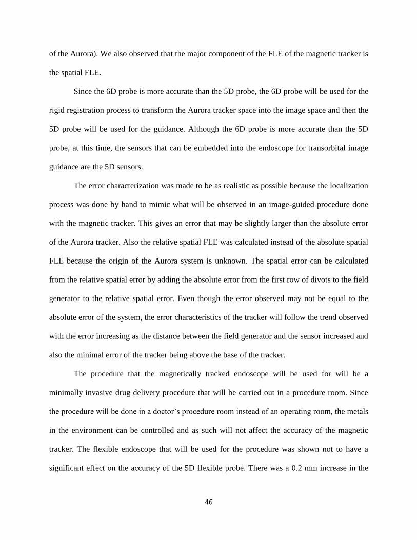
of the Aurora). We also observed that the major component of the FLE of the magnetic tracker is

the spatial FLE.

Since the 6D probe is more accurate than the 5D probe, the 6D probe will be used for the

rigid registration process to transform the Aurora tracker space into the image space and then the

5D probe will be used for the guidance. Although the 6D probe is more accurate than the 5D

probe, at this time, the sensors that can be embedded into the endoscope for transorbital image

guidance are the 5D sensors.

The error characterization was made to be as realistic as possible because the localization

process was done by hand to mimic what will be observed in an image-guided procedure done

with the magnetic tracker. This gives an error that may be slightly larger than the absolute error

of the Aurora tracker. Also the relative spatial FLE was calculated instead of the absolute spatial

FLE because the origin of the Aurora system is unknown. The spatial error can be calculated

from the relative spatial error by adding the absolute error from the first row of divots to the field

generator to the relative spatial error. Even though the error observed may not be equal to the

absolute error of the system, the error characteristics of the tracker will follow the trend observed

with the error increasing as the distance between the field generator and the sensor increased and

also the minimal error of the tracker being above the base of the tracker.

The procedure that the magnetically tracked endoscope will be used for will be a

minimally invasive drug delivery procedure that will be carried out in a procedure room. Since

the procedure will be done in a doctor’s procedure room instead of an operating room, the metals

in the environment can be controlled and as such will not affect the accuracy of the magnetic

tracker. The flexible endoscope that will be used for the procedure was shown not to have a

significant effect on the accuracy of the 5D flexible probe. There was a 0.2 mm increase in the

47

RMS error between the sensor and the sensor–endoscope configuration. The error observed

incorporates both the repositioning error and the error due to the effect of the flexible endoscope.

Therefore the error due to the endoscope may be less than 0.2 mm.

One of the advantages of transorbital endoscopic procedures is the fact that the orbit is a

small space and FLE of the tracker do not degrade as much in the working volume required for

the procedure. This was evidenced in the calculations of the FLE for the different field generator

positions shown in Figure 9. For the different field generator placements we found an average

random FLE to be less than 0.06 mm for the 6D probe and 0.2 mm for the 5D probe. We also

observed an average relative spatial FLE of less than 0.7 mm for the 6D probe, 1.3 mm for the

5D probe. We plan on incorporating these findings in the placement of the Aurora field generator

during the image-guided transorbital procedure.

References

1. Zhang, H., et al., Electromagnetic tracking for abdominal interventions in computer

aided surgery. Computer Aided Surgery, 2006. 11(3): p. 127-136.

2. Wood, B.J., et al., Navigation with Electromagnetic Tracking for Interventional

Radiology Procedures: A Feasibility Study. Journal of Vascular and Interventional

Radiology, 2005. 16: p. 493-505.

3. Krucker, J., et al., Electromagnetic tracking for thermal ablation and biopsy guidance:

clinical evaluation of spatial accuracy. Journal of Vascular & Interventional Radiology,

2007. 18(9): p. 1141-50.

4. Hummel, J.B., et al., Evaluation of a new electromagnetic tracking system using a

standardized assessment protocol. Physics in Medicine and Biology, 2006. 51: p. N205-

N210.

5. Frantz, D.D., et al., Accuracy assessment protocols for electromagnetic tracking systems.

Physics in Medicine and Biology, 2003. 48(14): p. 2241.

48

6. Mark A. Nixon, B.C.M., W. Richard Fright and N. Brent Price, The Effect of Metals and

Interfering Fields on Electromagnetic Trackers. Presence, MIT Press, 1998. 7(2): p. 204-

218.

7. Hummel, J.B., et al., Design and application of an assessment protocol for

electromagnetic tracking systems. Medical Physics, 2005. 32(7): p. 2371-2379.

8. Fitzpatrick, J.M., J.B. West, and C.R. Maurer, Jr., Predicting error in rigid-body point-

based registration. Medical Imaging, IEEE Transactions on, 1998. 17(5): p. 694.

9. Wilson, E., et al., A hardware and software protocol for the evaluation of

electromagnetic tracker accuracy in the clinical environment: a multi-center study.

Medical Imaging 2007: Visualization and Image-Guided Procedures: Proc. of SPIE,

2007. 6509: p. 65092T-1-11.

49

CHAPTER IV

MANUSCRIPT 2- Sensitivity analysis of fiducial placement on transorbital target registration

error.

Atuegwu N C and Galloway R L

Original form of manuscript appears in IJCARS Volume 2, Number 6 April, 2008, pages 397-

404

Abstract

Objective In many clinical applications of image-guided surgery, skin fiducial placement is

poorly defined and occasionally poorly executed, leading to an increase in the target registration

error (TRE). Fiducial placement analysis usually focuses on a single target, where surgical

guidance requires accurate localization of a region or volume of tissue. To address these

limitations, a method of fiducial positioning for minimizing the TRE in a target region was

developed.

Method This methodology uses patient specific anatomic data, the patient skin surface and

accounts for areas which may be poor choices for fiducial placement due to likely fiducial

motion. The effect of skin motion on the expected TRE of a target region was modeled and

evaluated. Transorbital therapy delivery was selected as the application of interest, so facial

morphology is of greatest importance. Our target region is the pyramidal space behind the globe

of the eye. A laser range scan of the face of a skull phantom with taboo regions chosen

semiautomatically was used as an input to the simulated annealing optimization algorithm.

Results Optimizing the fiducial position reduced the expected TRE by 50% when compared to an

unoptimized fiducial placement. In addition, the effect of fiducial motion or localizer fiducial

localization error is also reduced in the optimized version.

50

Conclusion Improved registration results for transorbital therapy delivery were achieved

semiautomatically using optical facial surface scans for image-guided surgical localization. The

target registration error minimization method was feasible for in vivo applications.

Introduction

Image guided surgery (IGS) requires a registration between an object in physical space

and the same object in image space. The most common method of registration used for IGS is

point based registration. The most effective point based registration uses extrinsic objects that are

attached to patients such extrinsic objects or anatomic landmarks are referred to as fiducial

markers.

The quality of fiducial-based registration may be judged by several types of registration

error computed after the registration. The three main measures of registration are fiducial

localization error (FLE), fiducial registration error (FRE) and target registration error (TRE).

FLE is the error in locating the position of a fiducial in any space. FRE is the distance between

corresponding fiducial points after registration. TRE is the distance between the corresponding

―target‖ points after registration. ―Target‖ in this case means points other than the fiducial points

[1]. FLE is affected human error in the placement of the tracking probe during localization of the

fiducials and the error associated with the tracking system [2].

Two basic types of fiducial markers are used in neurosurgical IGS: bone implantable

markers [3] and skin surface fiducials [4]. Bone implanted fiducials generally are more invasive

and cannot be used for procedures that are repetitively done on a patient. Skin fiducials are not

invasive and can be used frequently on a patient. Since skin moves over the bone, skin fiducials

are by nature, more mobile than bone implantable markers, and this may lead to an increase in

51

the localization error of the skin fiducials. This increase in localization error leads to an increase

in TRE during the IGS procedure.

Fiducial registration theory is based on localization of the fiducial points and several

presumptions. These presumptions are that extrinsic objects that define the fiducial points do not

move relative to the anatomy of the patient and other markers, the surgical target is a constant

point and that all positions for markers have equal likelihood or utility.

The paper deals with the fact that the target is rarely a point but a region. It also deals

with motion of skin fiducials relative to both the anatomy of the patient and to other fiducials. It

also deals with the fact that there are positions where the fiducials cannot be applied on the

patient and that all positions of markers do not have equal utility. The places where the fiducials

cannot be applied to are referred to as the ―taboo‖ regions. Also the fiducials have physical

constraints such as the size and the shape of the fiducial that further affect the placement of the

fiducials.

Optimizing the fiducial arrangement can decrease the TRE obtained after registration.

This is especially important when the target is a target zone as opposed to a target point and

when the FLE of the system is high; as in the case of a magnetic tracker, which has shown FLE

values of about 1-10mm in parts of the work volume [5, 6]. Also skin motion can lead to a

further increase in FLE during registration. Optimal placement of the skin fiducials in less

mobile parts of the skin and the avoidance of areas that may be deformed or shifted during the

imaging and surgical procedure can lead to a reduction in the overall FLE associated with skin

fiducials [1].

Several groups have shown that the arrangement of fiducials before point based

registration affects TRE obtained after registration[1, 7, 8] West et al proposed some guidelines

52

for fiducial placement given a certain target[1]. Liu et al showed an improvement in TRE by

optimizing random skin fiducial positions used during photogrammetry based patient positioning

systems. In both cases, the groups did not take into account patient specific geometry, the areas

that the fiducials cannot be placed on due to obstruction of the surgeons view and also areas that

are more likely to move when skin fiducials are placed.

The purpose of this paper is to present a semiautomatic method of fiducial positioning for

minimizing the TRE in a target region subject to the surgical space available and parts of the

surface that are less liable to skin motion. This removes the guesswork in image placement for a

particular patient. The paper also explores the effect of skin motion or fiducial localization errors

on TRE in a target zone. Our laboratory has been working on image guided endoscopic drug

delivery to the optic nerve therefore the paper will specifically explore the minimization of the

TRE in the region occupied by the optic nerve eye junction. In the case of image guided

endoscopic drug delivery, the procedure will be done multiple times a year and as such requires

skin fiducials. Also a magnetic tracker will be used for the endoscopic guidance. Since the FLE

associated with a magnetic tracker is high, an optimization of fiducial placement is essential.

Materials and Methods

TRE analysis

Equation 9 shows the relationship between TRE, FLE and the number and position of

fiducials used for the registration [7]

22 2

2 21

1 1 K Ki

i j i ii jj

rTRE r FLE

N K 2

Number of fiducials

Spatial dimension; K=3

Distance between the centroid of the fiducials and the target

=Eigenvalues of the fiducial arrangement

i

N

K

r

53

To minimize the TRE at a target point, equation 9 above has to be minimized. From

equation 9, the number of fiducials and the FLE can be assumed to be constant; therefore the

minimization of the rotational component of the TRE minimizes expected TRE.

Therefore,

22

2 21

1min min

K Ki

i j i ii jj

rTRE r R r

K 3

To minimize the objective function R(r), simulated annealing (SA) was used. SA

employs a random search which not only accepts changes that decrease the objective function

but also some changes that increase it. SA's major advantage over other methods is an ability to

avoid becoming trapped in local minima. The disadvantage of SA is that it can be computational

expensive as the algorithm can keep ―bouncing around‖ as probabilities that can increase the

objective function can be chosen. An optimized simulated annealing method from Bohachevsky

et al[9] was used. This reduced the computational time by introducing variables that controlled

the acceptance of probabilities as the solution neared the global optimum. Also since SA

involves a probabilistic method, a slightly different answer can be obtained for the same

optimization function.

SA Algorithm pseudocode

1. Initial positions for all the fiducials are chosen. 0 1 2 3, , .... NX x x x x ; N is the number of

fiducials used. The initial positions are chosen to be in the regions other than the avoid

regions. This is the input to the algorithm.

2. x is the function to be minimized; m is the value at the minimum

3. Find the nearest rd neighbors to 0X . rd is the region that the SA algorithm search can

move to for the next search.

54

4. 0 0X . If 0 m stop

5. Random direction. Get a random neighbor from rd points and use that as the new

direction. Generate new values 1X .

6. If any component of 1X is in the taboo or no overlap zone. Go back to 5. Otherwise set

1 1X and 1 0 . Do this for a fixed number and then choose a new

random point from the surface if 1X is still in taboo region.

7. 1 0 , set 0 1X X and 0 1 . If 0 m stop otherwise go the step 3.

8. If 1 0 , set 0exp gp . (a) Generate a uniform 0-1 random number V. (b) If

V p go to step 5. (c) If V p set 0 1X X and 0 1 ; and go to step 3.

9. Do 1-8 above until the maximum number of iterations is reached.

The variable is a positive number that is chosen so that p is between 0.5 and 0.7. This

prevents very few or all the searches from being accepted and g is an arbitrary negative

number that makes the probability of accepting a detrimental step tend to zero as you

approach the global extremum.

The algorithm minimizes the objective function until an acceptable tolerance value is

reached or the algorithm reaches the maximum number of iterations and the minimal rotational

error obtained during the search is used. Since the minimum rotational error that can be obtained

is zero, the tolerance value was chosen to be close to zero. A value of 1e-3 was chosen as the

tolerance value because from equation 9, 1

N

for the procedure is at least one magnitude less than

1e-2 and therefore adding a value of less than 1e-3 to the 1

N

term is not significant.

55

Target for the optimization

Our laboratory has been working on developing a system for drug delivery to the optic

nerve. In the case of transorbital drug delivery, the main target is the optic nerve eye junction.

Therefore the potential error in delivering a drug to the optic nerve eye junction needs to be

determined.

Since the optic nerve moves with eye motion, the optic nerve junction cannot be assumed

to be stationary and thus the TRE calculations for a stationary target cannot accurately describe

the TRE that will be expected after registration in the optic nerve eye junction. To incorporate

the optic nerve eye junction in the optimization scheme the path of the optic nerve junction has

to be characterized. This was done by using the average maximum ocular duction of the eye and

the motion of the optic nerve in mm for each degree movement of the eye.

The mean of the maximum ocular duction between age groups of 14-95 was shown to be

54o for abduction, 44

o for adduction, 46

o for supraduction and 51

o for infraduction [10]

Abduction is the outward movement of the eyeball, adduction is the inward movement of the

eyeball, supraduction is the elevation of the eyeball and infraduction is the depression of the

eyeball.

Magnetic resonance imaging-dynamic color mapping was used by Abramoff et al to

calculate the motion of the optic of some healthy adult volunteers and they found that on the

average the optic nerve moved an average of 0.16mm per degree[11] The optic nerve motion can

then be calculated by multiplying the average optic nerve motion by the mean of the maximum

ocular duction. This is shown in equation 11 below.

56

( , , , ) ( , , , )( ) _ _ * _ _

abduction

adduction

supraduction

infraduction

ab ad su in ab ad su inRadius r mean ocular duction motion optic nerve

ab

ad

su

in 4

This gives the maximum path transversed by the optic nerve junction during gaze. This

maximum path will then be used for further TRE optimization calculations.

The orbit is roughly a quadrilateral pyramid with rounded angles, resembling a pear [12].

The space occupied by the eyeball optic nerve junction can be modeled as a cross section of the

―pear shaped‖ orbit at a distance from the base or opening of the orbit. This can be approximated

to a circle because the eyeball does not translate forwards but just moves side to side.

The radius of the circle can be approximated to be 7.5mm. This was calculated using

equation 11 above. This gives the target region for the optic nerve eye junction. The target is

chosen as a region that is 24mm from the surface of the eyeball. This corresponds to the average

size of the human eyeball [13]. Figure 13 shows a cartoon of the target region.

For the fiducial optimization, the target zone is discretized by randomly selecting 300

points in the target zone. This was done to simulate the different possible positions of the optic

nerve eye junction in the target zone. The average rotational error in the region is the evaluation

of the objective function in equation 10.

Surface Acquisition

To optimize the fiducial placement, the surface of the face of a skull phantom was

obtained using a laser range scan. A laser range scanner acquires three dimensional geometry of

an object by scanning a laser across an object. A calibrated geometry exists between the plane of

laser light and the camera. By triangulating between the observed laser image and the known

57

laser plane, a three dimensional point cloud representing the surface of the object is recovered.

The point cloud obtained is then used as an input into the optimization algorithm

Fiducial Avoid regions

In reality, there are areas of the face on which fiducial cannot be placed on such as the

eyelids. The regions are known as the ―taboo regions‖. A semi automatic method is used to

choose these regions. Taboo regions can also be chosen to encompass other regions that the

surgeon needs unobstructed during the interventions, regions that are more likely to be subject to

skin motion or some patient specific regions. For the simulation, the eyelids and other parts of

the face where a skin marker cannot be comfortably put on like tip of the nose and areas of the

skin that were prone to skin motion was chosen as the taboo region.

Additionally since the fiducials have a finite size, a region around each fiducial that

corresponds to the size of skin markers (20mm) called the ―no overlap region‖ was automatically

chosen during the calculations to avoid fiducial overlap. The ―no overlap regions‖ simulates the

condition found in real skin marker positioning.

58

Figure 13: Cartoon of the target region. The stars show the target region and some of the

possible locations of the target.

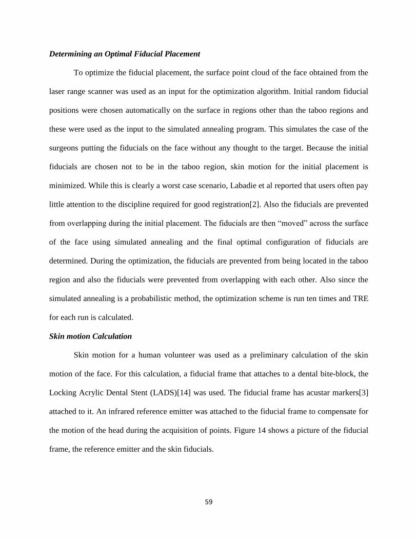
59

Determining an Optimal Fiducial Placement

To optimize the fiducial placement, the surface point cloud of the face obtained from the

laser range scanner was used as an input for the optimization algorithm. Initial random fiducial

positions were chosen automatically on the surface in regions other than the taboo regions and

these were used as the input to the simulated annealing program. This simulates the case of the

surgeons putting the fiducials on the face without any thought to the target. Because the initial

fiducials are chosen not to be in the taboo region, skin motion for the initial placement is

minimized. While this is clearly a worst case scenario, Labadie et al reported that users often pay

little attention to the discipline required for good registration[2]. Also the fiducials are prevented

from overlapping during the initial placement. The fiducials are then ―moved‖ across the surface

of the face using simulated annealing and the final optimal configuration of fiducials are

determined. During the optimization, the fiducials are prevented from being located in the taboo

region and also the fiducials were prevented from overlapping with each other. Also since the

simulated annealing is a probabilistic method, the optimization scheme is run ten times and TRE

for each run is calculated.

Skin motion Calculation

Skin motion for a human volunteer was used as a preliminary calculation of the skin

motion of the face. For this calculation, a fiducial frame that attaches to a dental bite-block, the

Locking Acrylic Dental Stent (LADS)[14] was used. The fiducial frame has acustar markers[3]

attached to it. An infrared reference emitter was attached to the fiducial frame to compensate for

the motion of the head during the acquisition of points. Figure 14 shows a picture of the fiducial

frame, the reference emitter and the skin fiducials.

60

Seven skin fiducials were attached to the patient at different positions on the face. An

optical tracker (Optotrak 3020 series, NDI Waterloo) with an infrared probe was used to localize

the fiducials. The positions of the fiducials were localized eleven times per fiducial with varying

random pressures applied on the fiducials during the fiducial localization. These moved the

fiducials on the skin during the fiducial localization process. This was done to stimulate the

possible fiducial motion that can happen during fiducial localization for image registration. The

bone fiducials were also localized and these were used as a comparison to identify the maximum

component of the error due to the optical localizer and the use of the reference emitter.

The mean of the 11 points per fiducial was calculated and the root mean square distances

of those points from the mean was calculated. This was also done for the acustar fiducials.

61

Figure 14: Picture of the face with the skin fiducials and the LADS with reference frame

attached.

62

Sensitivity Analysis of effect of skin motions and errors in fiducial placement on the TRE in

the target zone

Given that the bounds of the skin motion have been experimentally determined we could

perform simulations Skin motion was simulated by applying random vectors of different

magnitudes on the fiducials. Random vectors were used because the preliminary data for the skin

motion experiment showed that the fiducial measurements were uncorrelated in the both the x

and the y dimensions. The random vectors were applied to both the optimized and the

unoptimized fiducial positions. The random vectors encompass both the random and the biased

motions of the skin because in some cases the skin may be moved in a biased way. The

magnitude of the random vectors ranged from 1mm to 10mm. This range was found to be in

accordance with the range of errors error obtained from the deviation of skin fiducial localized

points from the mean of the data for each fiducial. The newly calculated fiducial position is then

used to calculate the expected TRE in the target region. For the simulation, the fiducials are

prevented from overlapping with each other but are allowed to be in any region around the face.

This simulates the possible motion of the skin or the possible error of the localizer in localizing

the position of the fiducials.

To simulate the effect of skin motion on the expected TRE in the target zone, 500

targets are chosen randomly in the target zone. The different fiducial positions produced by the

random application of the errors of different magnitudes to both the initial and the final fiducials

positions were used to calculate the TRE of all the 500 different targets in the target zone. For

each skin motion magnitude, 1000 random vectors for the skin motion are calculated and added

to both the optimized and the unoptimized fiducial positions. The average TRE for each

magnitude is then calculated across the different random skin motion. The above procedure was

63

repeated with the optimized fiducial positions obtained from running the algorithm ten times.

The average expected TRE across the different optimized fiducial results was then calculated.

Results

Figure 15a shows the result of the optimization algorithm. The squares are the initial

fiducial positions and the round dots are the final fiducial positions. Figure 15b shows the point

cloud of the skull phantom obtained from the laser range scan of the skull phantom face. The

dark regions in Figure 15b are the taboo regions that are avoided during the optimization process

but are included during the sensitivity analysis process. The mean value of the expected TRE for

the 10 trials for the unoptimized fiducial configuration for FLE of 1mm was 0.81± 0.04mm and

was 1.62 ± 0.08 for FLE of 4mm. The mean values for the <TRE> for the 10 trials for the

optimized fiducial position for an FLE of 1mm was 0.48 ± 0.01mm and was 0.96 ± 0.02 for FLE

of 4mm.

The results of the skin motion experiment are shown in table 9. The range of fiducial

motion observed was from 1-8mm with the highest motion occurring in fiducial 7 which is

located on the cheek. An average value of 0.21±0.11 mm RMS error was found for the bone

markers. This shows the error due to the optical localizer system used.

64

Figure 15: a) Skull phantom with the initial and final fiducial positions. The squares are the

initial fiducial position and the circles are the final fiducial position. b) Laser range scan of the

skull phantom with the taboo regions.

65

Table 9: The mean, standard deviation and the maximum values of the RMS distance of the

localized fiducial points from the mean of the distances.

66

Figure 16 shows the expected TRE of the target region for an FLE of 1mm for both the

optimized and the unoptimized fiducial position. The mean values for the ten trials was obtained

for the optimized fiducial location and plotted. From Figure 16 it can be observed that optimizing

the fiducials lead to a reduction of the expected TRE in the target region by about 50%. Also the

figure shows that the <TRE> increases more in the case of the unoptimized fiducial

configuration when compared to the optimized fiducial configuration as the magnitude of the

perturbation increases.

The standard deviation of the expected TRE in the unoptimized fiducial placement is

larger than the standard deviation of the expected TRE values in the optimized fiducial case. This

increase indicates an increase in the maximum observed TRE in the target region for the

unoptimized fiducial. There is also an increase in the standard deviation of the TRE values in the

unoptimized and optimized fiducial region as the magnitude of perturbation increases. Figure 17

shows the TRE calculated in the target region for an FLE of 4mm. The TRE increased as the

FLE increased from 1 to 4mm. The expected TRE decrease from unoptimized to optimized

fiducial position was still 50% and the standard deviation was still higher in the unoptimized vs.

the optimized fiducial.

67

Figure 16: TRE calculated in the target region for FLE value of 1mm for an initial naïve initial

fiducial position

68

Figure 17: TRE calculated in the target region for FLE value of 4mm for an initial naïve initial

fiducial position.

69

Since simulated annealing can produce different results for the same initial conditions,

the simulated annealing algorithm was run ten times for different random placements of the

fiducial and the sensitivity analysis of the region was done for the different results of the

simulated annealing program.

The average TRE in the target region for the ten different runs for the simulated

annealing program was calculated. Figure 18 shows the TRE of the region for the ten different

runs of the simulated annealing program for an FLE of 1mm. From the figure, it can be observed

that the simulated annealing program converges to roughly the fiducial placement that gives a

similar TRE on the average in the target region. Also in all cases of the simulation the TRE

obtained from the random motion was greater than the TRE from the optimized region and the

TRE for the random placement varied widely between simulations with the TRE in a simulation

nine as much 2.4 times the TRE of the optimized region.

70

Figure 18: Average TRE in the target region for ten different simulations of the simulated

annealing program

71

Discussion

In this paper, we developed a system to place fiducials on the surface of the face in order

to improve the expected TRE and also reduce the sensitivity of small amounts of marker motion

on the expected TRE in a target region. Boundaries on marker motion were set using

experiments conducted on a human subject. These boundaries were then used to test the

sensitivity of the optimized fiducial position to perturbations on the marker position. Simulated

annealing was used to optimize the fiducial configuration because of its ability to avoid being

trapped in local minima. The optimized fiducial configuration will be used for a magnetically

tracked endoscopic transorbital procedure.

The algorithm developed produces an optimized fiducial position that is patient specific.

It incorporates the surface structure of the patients, the taboo regions that encompass places that

are most likely to move or regions that the physician wants unobstructed during the image

acquisition process and the image guided procedure.

Skin fiducials although are more subject to motion than bone implanted fiducials, can

provide adequate registration for frequently repeated procedure such as drug delivery to the optic

nerve. The results show that regardless of the magnitude of the skin motion, an optimized

fiducial placement will help reduce the effect of skin motion and the error in fiducial

localization.

In this paper we used a phantom to study the effect of the optimization of fiducial

position on the expected TRE in a target region. While this application is based on phantom data,

we have used bounds developed from human data and plan to expand this test immediately into

two areas. First we will use anthropomorphic phantoms with real targets to get true TRE and

72

second we will perform on cadavers for true anatomy. We also plan on working on a way to

effectively place the fiducial on the skin after the fiducial positions are calculated.

References

1. West, J.B., et al., Fiducial Point Placement and the Accuracy of Point-based, Rigid Body

Registration. Neurosurgery, 2001. 48(4): p. 810-817.

2. Labadie, R.F., B.M. Davis, and M.J. Fitzpatrick, Image-guided surgery:what is the

accuracy. Current opinion in Otolaryngology & Head and Neck Surgery, 2005. 13: p. 27-

31.

3. Maurer, C.R., Jr., et al., Registration of head volume images using implantable fiducial

markers. IEEE Trans Med Imaging, 1997. 16(4): p. 447–462.

4. Barnett, G.H., D.W. Miller, and J. Weisenberger, Frameless stereotaxy with scalp-

applied fiducial markers for brain biopsy procedures: experience in 218 cases. Journal of

Neurosurgery, 1999. 91(4): p. 569-576.

5. Atuegwu, N., L. Mawn, and R.G. Jr, Transorbital Image Guidance, in IEEE EMBS.

2007: Lyon France.

6. Johann Hummel, et al., Design and application of an assessement protocol for

electromagnetic traking systems. Med Phys, 2005. 32(7): p. 2371-2379.

7. Fitzpatrick, J.M., J.B. West, and C.R. Maurer, Jr., Predicting error in rigid-body point-

based registration. Medical Imaging, IEEE Transactions on, 1998. 17(5): p. 694.

8. Liu, H., et al., Optimal marker placement in photogrammetry patient positioning system.

Medical Physics, 2002. 30(2): p. 103-110.

9. Bohachevsky, I., O., M. Johnson, E., and M. Stein, L., Generalized Simulated Annealing

for Function Optimization. Technometrics, 1986. 28(3): p. 209-217.

10. Shechtman, D., et al., Maximum Angle of Ocular Duction During Visual Fixation as a

Function of Age. Strabismus, 2004. 13(1): p. 21.

11. Abramoff, M.D., W.J. Niessen, and M.A. Viergever, Objective quantification of the

motion of soft tissues in the orbit. Medical Imaging, IEEE Transactions on, 2000. 19(10):

p. 986.

12. Dutton, J.J., Atlas of Clinical and Surgical Orbital Anatomy. 1994: W.B Saunders

Company.

73

13. Jordan, D. and R. Anderson, Surgical Anatomy of the Ocular Adnexa: AClinical

Approach. Opthalmology Monographs. 1996.

14. Labadie, R.F., et al., Submillimetric target-registration error using a novel, non-invasive

fiducial system for image-guided otologic surgery. Computer Aided Surgery, 2004. 9(4):

p. 145-153.

74

CHAPTER V

MANUSCRIPT 3- Image guided transorbital endoscopic procedure in phantoms

Atuegwu N.C, Mawn L and Galloway R.L

Manuscript in review in IEEE Transaction in Biomedical Engineering.

Abstract

Transorbital endoscopic procedures are hindered by the visual similarity of orbital

structures and that traditional orbital landmarks are lost during the procedure. These problems

can be addressed with the use of image guidance.

Image guided transorbital endoscopic guidance was carried out in anthromorphic

phantoms. 5mm stellate balls were used for both the targets and as distracters. The targets were

made radioopaque and attached to the orbit in close proximity to the distracters. White five mm

stellate balls were used to mimic orbital fat and were used to obstruct the view of both the target

and distracters. The targets were localized by three surgeons using a magnetic tracker attached to

a flexible endoscope.

The surgeon with the highest skill level correctly identified the target 100% of the time.

The fellow and the resident surgeons identified the targets correctly with image guidance 90% of

the time and correctly without image guidance 70% of the time. The surgical attending and

resident were faster with image guidance and the surgical fellow was equally as fast with image

guidance. These results show a potential increase in accuracy and a decrease in time of the

procedure by adding image guidance to transorbital procedures.

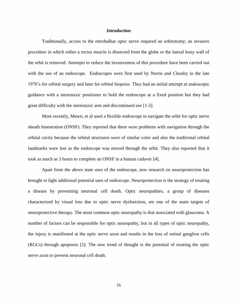
75

Introduction

Traditionally, access to the retrobulbar optic nerve required an orbitotomy; an invasive

procedure in which either a rectus muscle is dissected from the globe or the lateral bony wall of

the orbit is removed. Attempts to reduce the invasiveness of this procedure have been carried out

with the use of an endoscope. Endoscopes were first used by Norris and Cleasby in the late

1970’s for orbital surgery and later for orbital biopsies. They had an initial attempt at endoscopic

guidance with a stereotaxic positioner to hold the endoscope at a fixed position but they had

great difficulty with the stereotaxic arm and discontinued use [1-3].

More recently, Mawn, et al used a flexible endoscope to navigate the orbit for optic nerve

sheath fenestration (ONSF). They reported that there were problems with navigation through the

orbital cavity because the orbital structures were of similar color and also the traditional orbital

landmarks were lost as the endoscope was moved through the orbit. They also reported that it

took as much as 3 hours to complete an ONSF in a human cadaver [4].

Apart from the above state uses of the endoscope, new research on neuroprotection has

brought to light additional potential uses of endoscope. Neuroprotection is the strategy of treating

a disease by preventing neuronal cell death. Optic neuropathies, a group of diseases

characterized by visual loss due to optic nerve dysfunction, are one of the main targets of

neuroprotective therapy. The most common optic neuropathy is that associated with glaucoma. A

number of factors can be responsible for optic neuropathy, but in all types of optic neuropathy,

the injury is manifested at the optic nerve axon and results in the loss of retinal ganglion cells

(RGCs) through apoptosis [5]. The new trend of thought is the potential of treating the optic

nerve axon to prevent neuronal cell death.

76

Most of the common method of ocular drug deliveries do not effectively get the drugs to

the optic nerve axon and may have additional side effects. A system that can guide an endoscope

to the optic nerve for drug delivery can potentially be used for delivery of neuroprotective drugs

to the optic nerve cells.

For orbital endoscopic procedures to be used, the problem of navigation through the

orbital fat has to be improved since the orbital fat obscures easy visualization of optic nerve. This

problem can be solved with the use of image guidance during the endoscopic procedure.

Image Guided Surgery and Interventions (IGS)

Image guided surgery and interventions involve the use of medical images to select, plan

and guide a surgical procedure or medical intervention. Image guided surgery is based upon

integration of the preoperatively acquired and processed 3D information such as an image

volume of the patient and the corresponding anatomy of the patient within the same frame of

reference. Links between these two components are realized by combining image space to

patient space registration and by tracking instruments within the operational field.

The most common method of registration used for IGS is point based registration.

Extrinsic point based registration requires fiducials attached to patients. Two basic types of

fiducial markers are used in neurosurgical IGS: bone implantable markers [6] and skin surface

fiducials [7]. Bone implanted fiducials, while providing greater accuracy, are more invasive and

cannot be used for procedures that are repetitively done on a patient. Skin fiducials are not

invasive and can be used frequently on a patient. We chose skin fiducials for our work because

we envision the procedure being an outpatient procedure done multiple times a year and, as such,

bone affixed fiducials will not be suitable. The fiducials are used to register the image space to

77

the physical space. After the registration of the two images, the surgical or interventional

instruments have to be tracked within the operational field with a localizer.

Tracking a flexible endoscope in the operational field requires a localizer that does not rely on a

line of site between the camera and the sensor. A Magnetic tracker offers this advantage and thus

was selected for our work. Different groups have used magnetic trackers for imaging guided

procedures [8-10]. This can be attributed to newer generations of electromagnetic trackers that

show both an increased accuracy and have a reduced sensor size[11] making them easier to

embed in instruments. A disadvantage of magnetic localizers is that they induce eddy currents in

nearby conductive materials. These eddy currents create an opposing magnetic field to the

original external magnetic field. The intersection of the Aurora’s magnetic field with the

opposing magnetic field disrupts the magnetic field and can affect the transformation data

produced. This leads to systematic tracking errors. Careful placement of the magnetic transmitter

and the magnetic sensor in relation to the metals in the environment can help reduce the amount

of error in the measured position of the sensor[12]. There are several commercially available

magnetic localizers and for this work the Aurora system (Northern Digital Inc, Waterloo,

Ontario) was used.

Before a localizer can be effectively used for image guided procedures, a characterization of the

localizer is required. A volumetric characterization of the FLE in the working volume of the

Aurora magnetic tracker by sampling the magnetic field using a tomographic grid was performed

by our lab [13]. The Aurora error characterization was performed by moving the flat plexi-glass

phantom up in height in increments of 38.4mm from 9.6mm to 201.6mm. The final stopping

distance was chosen to correspond to the average size of the human head. For each plane, a 5D

and a 6D sensor was used to localize each divot and the random and the relative spatial FLE of

78

each plane was calculated. For different positions of the magnetic tracker from the object the

random and spatial FLE was calculated. Different experimental setups shown in Figure 19 were

proposed in our previous work[13]. For this paper we chose the setup in A shown in Figure 19.

Based on the experimental setup A, the average random FLE was 0.034±0.017mm for the 6D

probe and 0.127± 0.063mm for the 5D probe and the average spatial FLE for the six planes is

0.40±0.27mm for the 6D probe and 0.86 ±0.42mm for the 5D probe. The effect of an endoscope

on the flexible 5D magnetic sensor was also carried out by localizing a divot without and without

the endoscope in contact with the sensor and measuring the deviation between the two

measurements. The endoscope deviation was shown to be 0.2mm.

79

Figure 19: Picture of the possible placements of the magnetic tracker[13]

80

Methods

The retroorbital area is filled with fat which surrounds the optic nerve and cushions the

eye. Targeting the optic nerve required penetration and transversal of the fat. The fat is confined

by the orbital septum which shapes and structures the orbital fat. The orbital fat is deformable

and can be penetrated. In order to have a penetrable material with a radiographically visible

target, our experimental design was to use 5mm white stellate balls that were deformable,

penetrable and visibly similar to fat as the orbital fat. We also used colored 5mm stellate balls

soaked in iodine based computed tomography (CT) contrast agent as the target. The eyeballs and

optic nerve were chosen based on size, distensibility and appearance to mimic their respective

tissues. A nylon white cord was selected to mimic the optic nerve. The cord was soaked in

iodine based CT contrast agent to make it radiopaque and was attached to the eyeball. The optic

nerve-eyeball configuration was then attached to a skull through the optic foramen. Prior to

soaking the targets in contrast agents, the target colors were randomly chosen from five possible

colors and the positions of the targets in the orbit were randomly chosen based on the four

quadrants of the orbit. Two additional colored balls were placed near the target to serve as

distracters. The distracters colors were colors other that those chosen for the target. Colored

targets and distracters were chosen to give color information to the endoscope and the

radioactive target was chosen to give radioactive visibility to the target during the image guided

procedure. The distracters were not soaked in iodine based contrast agent and as such were not

visible on a CT volume. The targets and distracters were rigidly attached to the orbit with the use

of white stellate balls attached to the boney orbit. This arrangement made the targets appear free

floating and more difficult to get to. After the target and distracters were attached to the orbit the

orbit was then filled up with the white stellate balls.

81

Figure 20: Picture of the experimental setup

82

Prior to the image guided (IG) procedure, skin fiducials were attached in an optimized

manner on the phantoms [14] and a CT scan of the skull was obtained. Figure 20 shows a

picture of the experimental setup with the eye of interest being the one closest to the Aurora

magnetic tracker.

A point based registration algorithm was used for the registration of the fiducials positions in the

image space and physical space. Image guidance was then performed using Operating Room

Image Oriented Navigation (ORION) software[15]. ORION is a PC-based surgical guidance

system which synchronously tracks and displays surgical position on up to four image sets and

updates them in real time.

A 5D magnetic tracker was rigidly attached to a Storz Flex –X2 (Karl Storz endoscopy

America Inc) flexible endoscope. The endoscope-sensor configuration was used to localize the

targets in the anthropomorphic phantoms. Prior to the target localization, the surgeons located

the target in a CT image volume and are allowed to make calculations and take notes. The

ORION four pane windows with three orthogonal views of the CT image in three planes and a

view of the endoscopic image in one of the plane is used for the localization during the image

guided part of the procedure. This is shown in Figure 21. For the non image guided part a

stationary image with the target shown is available on a computer screen. The surgeon was

allowed to consult the images during the procedure if they want clarification.

83

Figure 21: Screen shot of the ORION image guidance software used. The three planes show the

three orthogonal views of the skull phantom and the last plane shows the endoscopic view.

84

The task for the surgeons was to identify the color of the target with and without image

guidance. The time to target was recorded during the process. The order of surgeon experiment,

image guided and non image guided was chosen randomly. The targets in the orbits were

identified with either image guidance or non image guidance for the first trial. The opposite

guided state was then applied in a second trial. The two trials for each target were separated by a

week to prevent the surgeon from remembering the path to the target. The target correctness was

neither confirmed nor denied during the whole experiment so the surgeon was not aware of the

right answer. Twelve targets were localized by the attending surgeon (highest skill level), ten

targets were localized by the surgical fellow and the surgical resident.

Results

Two metrics – percentage correct identification and time to target were used to evaluate

the effect of image guidance. The times with the target correctly identified in both IG and non IG

procedure is compared to determine the efficacy of image guidance for the three doctors with

varying skill levels. Incorrect target identification is also recorded and analyzed. For the

attending surgeon with the highest skill level the time to target with image guidance was on the

average 2.5 times faster than the time to target without image guidance. The mean value for the

time to target with image guidance was 72 seconds and the mean value of the time to target

without image guidance was 163 seconds. The attending surgeon was able to locate the target

correctly with both IG and non IG in 100% of the cases. Figure 22 shows a graph of the non

image guided times vs. the image guided times. The line represents the time when image

guidance is equal to non image guidance. Image guided times was faster in 83% of the times for

the different target positions localized.

85

Figure 22: Graph of the non image guided times vs. the image guided times for the different

targets for the attending surgeon. The line represents the times when the time to target with

image guidance was equal to the time to target with non image guidance.

86

The results of the experiments for both the surgical resident and surgical fellow are

shown in Figure 23 and Figure 24. The graph showed the times when the surgeons correctly

identified the colored targets with both IG and non IG. The fellow and the resident surgeons

correctly identified the target with image guidance 90% of the time and correctly identified the

target with non image guidance 70% of the time. The fellow was faster with image guidance for

the correct targets 50% of the times and the resident was faster with image guidance for the

correct target 67% of the time. The results are summarized in Table 10.

87

Figure 23: Graph of the non image guided times vs. the image guided times for the different

targets for the surgical fellow.

88

Figure 24: Graph of the non image guided times vs. the image guided times for the different

targets for the surgical resident.

89

Table 10: The accuracy and the time of image guided and non image guided endoscopic phantom

studies

Discussion

Transorbital endoscopic guidance was carried out on anthromorphic phantoms. There

was an increase in the accuracy of the procedure especially in less skilled surgeons with image

guidance than without image guidance. Image guidance times were faster than non image

guidance times in the case of the attending surgeon and the resident surgeon. It performed

equally as fast as the non image guided times for the fellow. The discrepancy in the times found

for different targets was due to the fact that the targets were different and randomly selected and

this made some location was more difficult to get to than other location. Since the same target

was identified with both image guidance and non image guidance, the difficulty level is same for

the target but different across target. The above results show a potential benefit of image guided

endoscopic transorbital procedures.

Acknowledgement

This work was supported by the NIH grant # 4-22-430-0713. The authors will like to thank Dr

Cari Lyle and Dr Lillian Ringsdorf for their help with data collection. The authors will also like

to thank Karl Storz endoscopy America Inc for providing us with the endoscope. The authors

will also like to thank the CT tech in Vanderbilt medical center for help with imaging the

phantoms.

90

References

1. Norris JL, C.G., An endoscope for ophthalmology. American Journal of Ophthalmology,

1978. 85(3): p. 420-2.

2. Norris JL, S.W., Bimanual endoscopic Orbital Biopsy. Ophtalmology, 1985. 92(1): p. 34-

38.

3. Norris JL, C.G., Endoscopic orbital surgery. American Journal of Ophthalmology, 1981.

91(2): p. 249-252.

4. Mawn, L.A.S., Jin-Hui ; Jordan, David R.; Joos, Karen M. , Development of an Orbital

Endoscope for Use with the Free Electron Laser. Ophthalmic Plastic & Reconstructive

Surgery, 2004. 20(2): p. 150-157.

5. N Osborne, G.C., C J Layton, J P M Wood, R J Casson and J Melena, Optic nerve and

neuroprotection strategies. Eye, 2004. 18: p. 1075-1084.

6. Maurer, C.R., Jr., et al., Registration of head volume images using implantable fiducial

markers. IEEE Trans Med Imaging, 1997. 16(4): p. 447–462.

7. Barnett, G.H., D.W. Miller, and J. Weisenberger, Frameless stereotaxy with scalp-

applied fiducial markers for brain biopsy procedures: experience in 218 cases. Journal of

Neurosurgery, 1999. 91(4): p. 569-576.

8. Zhang, H., et al., Electromagnetic tracking for abdominal interventions in computer

aided surgery. Computer Aided Surgery, 2006. 11(3): p. 127-136.

9. Wood, B.J., et al., Navigation with Electromagnetic Tracking for Interventional

Radiology Procedures: A Feasibility Study. Journal of Vascular and Interventional

Radiology, 2005. 16: p. 493-505.

10. Krucker, J., et al., Electromagnetic tracking for thermal ablation and biopsy guidance:

clinical evaluation of spatial accuracy. Journal of Vascular & Interventional Radiology,

2007. 18(9): p. 1141-50.

11. Hummel, J.B., et al., Evaluation of a new electromagnetic tracking system using a

standardized assessment protocol. Physics in Medicine and Biology, 2006. 51: p. N205-

N210.

12. Mark A. Nixon, B.C.M., W. Richard Fright and N. Brent Price, The Effect of Metals and

Interfering Fields on Electromagnetic Trackers. Presence, MIT Press, 1998. 7(2): p. 204-

218.

91

13. Atuegwu, N.C. and R.L. Galloway, Jr, Volumetric characterization of the Aurora

magnetic tracker system for image guided transorbital endoscopic procedures. Physics in

Medicine and Biology, 2008.

14. Atuegwu, N.C. and R.L. Galloway, Sensitivity analysis of fiducial placement on

transorbital target registration error. International Journal of Computer Assisted

Radiology and Surgery, 2008. 2(6): p. 397-404.

15. Stefansic, J.D., et al., Design and implementation of a PC-based image-guided surgical

system. Computer Methods and Programs in Biomedicine 2002. 69(3): p. 211-224.

92

CHAPTER VI

SUMMARY

Transorbital endoscopic procedures are hindered by the orbital fat that prevents direct

visualization of the optic nerve. The addition of image guidance to transorbital procedures will

help address this problem. With image-guidance orbital structures can be localized in the

preoperatively obtained images and supplied to the surgeon via registration and an actively

tracked tool. Such an image guidance system requires a registration between the physical space

and the image space. A localizer is need for both the registration and the tracking of the object

after registration. For transorbital image guidance which requires non linear therapeutic paths , a

non-line of sight system such as a magnetic localizer is most appropriate. Magnetic tracking

systems have sensors that can be attached to the endoscopes to couple the live video with the

location displayed on the preoperative images. While the most appropriate localizer for this

application, magnetic localizers are inherently less accurate than optical localizers a volumetric

characterization of the error metrics is required. Chapter III presents this volumetric

characterization. The ―sweet spot‖ of the magnetic tracker is documented and this is used in the

placement of the magnetic tracker during endoscopic orbital procedures.

The registration accuracy metric, TRE, is affected by the placement of fiducials during

the registration. Chapter IV presents the optimization of fiducials to reduce the TRE in a target

region and the sensitivity analysis on the effect of fiducial localization error on the TRE. The

bounds of the error were quantified by skin motion error calculations. The results of the

optimization and the magnetic tracker characterization were used to quantify the benefits of

adding image guidance to transorbital endoscopic procedure.

93

Chapter V presents the accuracy and the timing results of adding image guidance to

transorbital endoscopic procedures in an anthromorphic phantom. The results show that image

guidance leads to a reduction of the time for the procedure and an increase in accuracy of the

procedure. Also surgeons reported a greater confidence in their results with image guidance.

Future work with respect to the work presented here will be validating the effects of

endoscopic image guidance in an animal model. The timing and accuracy in identifying targets

have to be quantified. Also further validation of the reduction of TRE with the use of optimized

fiducials has to be carried out both with phantoms and animals.

94

Appendix A

Accuracy measurement of the effect of some materials on the Aurora magnetic system

For image guided orbital endoscopic procedures, the role of the endoscope-magnetic

sensor system is to mostly traverse the orbital fat. A measurement of the effect of fat and fat like

materials on the sensor system is required in order to determine if there is error induced on the

sensor position by the presence of fat and fatty substances.

Method

Three materials, steel, mayonnaise and animal fat were cut in lengths of 4cm and glued to

a piece of wood. This prevents the movement of the materials during the measurement. A 5d

sensor was rigidly attached to a plexiglass piece. Baseline measurements were done with the 5d

sensors. The materials were then put within 5mm of the sensor and measurements were collected

again. For both the baseline and the measurements with the material 1000 points were collected.

The error due to the addition of the material was calculated by determining the difference of the

mean of the two measurements (baseline and measurement with material). Baseline

measurements were taken before any material was brought in close proximity to the sensor to

ensure that any movement or shift in the sensor is recorded. This is essential to insure that any

errors ascribed to the material were actually the result of the materials.

Results

The results of the experiment are shown in table 1 below. From table 1, the error due to

steel is 1.7931e+005 times more than the error due to animal fat. Also the error shown due to

animal fat is very close to the baseline mean and within the random error of the sensor.

95

Table 11: Errors and variances due to the different materials

Material

Error(mm)

Variances

Baseline(mm2) Measurement

with

material(mm2)

Steel 3.7606 0.0011 0.0016

Mayonnaise 4.6319e-005 0.0013 0.0015

Animal fat 2.0973e-005 9.2218e-004 0.0010

Discussion and conclusion

Since the deviation of the measurement with respect to the addition of fat is very small

and within the random error of the sensor, then fat does not introduce any deviation in measured

data versus those from measured in air. By using a material (steel) known to disturb the

localization, we confirm the validity of the experiment. The difference in the errors observed for

steel bolt and animal fat is due to the magnetic susceptibility of the two materials. Since the

medical application exposes the localizer to fat, not steel, we have confidence that our phantom

experiments with air based measurements predict the performance in patients.

96

APPENDIX B

Dealing with Correlated FLE

As seen in Chapter III, spatial FLE ( ) is a slowly varying function of space. This

means that there is in fact a strong correlation between the spatial component of FLE at each of

the fiducial points and indeed at the target. Measured FLE is composed of a random term

and a spatial component of the FLE . However, the FLE/FRE/TRE

theory developed by West and Fitzpatrick presumes that the FLE is uncorrelated across the

measurement zone. 2

2 2

2 21

1 1 K Ki

i j i ii jj

rTRE r FLE

N KThus the FLE used in the

minimization algorithm in Chapter IV was the . This is because the FLE has to be

spatially uncorrelated for the equation above to hold true. However, changes in the

also lead to changes in the TRE of the procedure. A quantification of the TRE increase due to

is required to know the total TRE that is expected during the procedure.

Method

The measurements that were obtained in Chapter III were overlaid with the skull

phantom used for the optimization method. The placement coincides with placement A shown in

figure 1 below. The skull phantom and the grid phantom were overlaid as shown in figures 2 and

3. To calculate the FLE of the fiducials and the target centroid, the nearest plane to the centroid

of the fiducials and the target and four the nearest grid points to the centroids of both the target

and the fiducial in the nearest plane was used. This was done for 10 optimized and unoptimized

fiducial positions and the translational TREs for the optimized fiducial positions were calculated.

If we assume that the optic nerve will be at the centroid of the fiducial configuration then the

97

rotational TRE is negligible, then the TRE due to the will be the translational

component of the TRE. The translational TRE due to is the difference between the

average , in each direction, at the fiducials, and the average , in each

direction, at the target.

Figure 25: The possible placements of the Aurora magnetic tracker relative to the head.

98

Figure 26: Overlay of the skull phantom and the grid phantom

Figure 27: Planar overlay of the grid phantom and skull phantom

99

Results

Table 1 shows the translational TRE between the target and the fiducials for ten optimized trial

runs. The average translational TRE is 0.2081± 0.1180mm and the maximum and minimum

translational TRE’s are 0.3667mm and 0.0794mm respectively.

Table 12: Translational TRE values for the optimized fiducial configuration

Fiducial

Configuration

1

2

3

4

5

6

7

8

9

10

TRE(mm) 0.361 0.140 0.367 0.114 0.122 0.321 0.322 0.108 0.080 0.148

Table 13: Translational TRE values for the unoptimized fiducial configuration

Fiducial

Configuration

1

2

3

4

5

6

7

8

9

10

TRE(mm) 0.468 0.628 0.667 0.491 0.494 0.317 0.686 0.560 0.588 0.574

Table 2 shows the results of the translational TRE for the unoptimized trial runs. The average

translational TRE is 0.547±0.110mm and the maximum and minimum translational TRE’s are

0.686mm and 0.317mm respectively.

Discussion

The optimized fiducial placement leads to both a reduction in the TRE due to the random

and . The increase in the translational TRE in the unoptimized position may be due to

the fact that the fiducials are placed in the region where the may be rapidly varying.