Ind

ust

rial E

lectr

ical En

gin

eerin

g a

nd

A

uto

matio

n

CODEN:LUTEDX/(TEIE-5279)/1-76(2011)

Estimation of Vehicle Roll Angle

Anthon NilssonHerman Lingefelt Division of Industrial Electrical Engineering and Automation Faculty of Engineering, Lund University

1

Preface

This thesis work has been done in cooperation with Haldex Traction AB in Landskrona and the Industrial Electrical Engineering and Automation (IEA) division at LTH, Lund. It has been carried out at the department of Haldex Traction AB in Landskrona during September 10 to January 11.

First and foremost we want to thank all people at Haldex Traction group who have helped us and made it a pleasant stay. We would especially want to thank Pierre Petterson for his time and contribution to this thesis. Furthermore many thanks go to both our advisors at Haldex; Christian Rylander and Tord Diswall. At IEA we would like to thank our supervisor and mentor Gunnar Lindstedt and also our examiner Ulf Jeppsson.

Sturup Raceway made it possible for us to test our algorithm in a banked curve on their raceway. Many thanks to them and Ted Brink who provided us with the contact to Sturup Raceway. Both authors have contributed equally to all parts in this thesis.

Lund, January 11 Anthon Nilsson and Herman Lingefelt

2

Contents

1. Introduction ................................................................................. 5

1.1 Background ........................................................................................... 5

1.2 Problem formulation ............................................................................. 6

1.3 Research objective ................................................................................ 7

1.4 Related work ......................................................................................... 7

2. Tools and conditions ................................................................... 8

2.1 MATLAB/Simulink - VehSim ................................................................... 8

2.2 Volkswagen Golf GTI ............................................................................. 9

2.3 Implementation .................................................................................. 10

2.4 Coordinate systems ............................................................................. 10

2.5 Summary ............................................................................................. 10

3. Theoretical solution................................................................... 11

3.1 Derivation of the equation for calculating road banking ...................... 11

4. Modeling ................................................................................... 17

4.1 Vehicle modeling overview.................................................................. 17

4.2 Bicycle model ...................................................................................... 17

4.3 Tire model ........................................................................................... 18

4.4 Matlab/Simulink model ....................................................................... 22

5. Observer techniques ................................................................. 30

5.1 Overview ............................................................................................. 30

5.2 Averaging observer ............................................................................. 31

5.3 Linear Kalman filter ............................................................................. 31

5.4 Extended Kalman filter ........................................................................ 35

6. Observer design ......................................................................... 37

6.1 Discretization ...................................................................................... 37

6.2 Extended Kalman filter ........................................................................ 39

6.3 Summary ............................................................................................. 42

7. Signal processing and error detection ....................................... 43

7.1 Signal processing ................................................................................. 43

7.2 Error detection .................................................................................... 45

7.3 Different roll angles ............................................................................. 61

8. Results ....................................................................................... 63

8.1 Model and observer ............................................................................ 63

8.2 Detection of errors and filtering .......................................................... 64

8.3 Simulation results ................................................................................ 64

3

8.4 Summary ............................................................................................. 67

9. Discussion and conclusion ......................................................... 68

9.1 Future work......................................................................................... 69

10. Nomenclature ......................................................................... 70

10.1 Expression explanation ........................................................................ 70

10.2 Physical units....................................................................................... 70

11. References .............................................................................. 71

12. Appendix A - Chassis roll reference estimation...................... 72

13. Appendix B - Vehicle model ................................................... 75

4

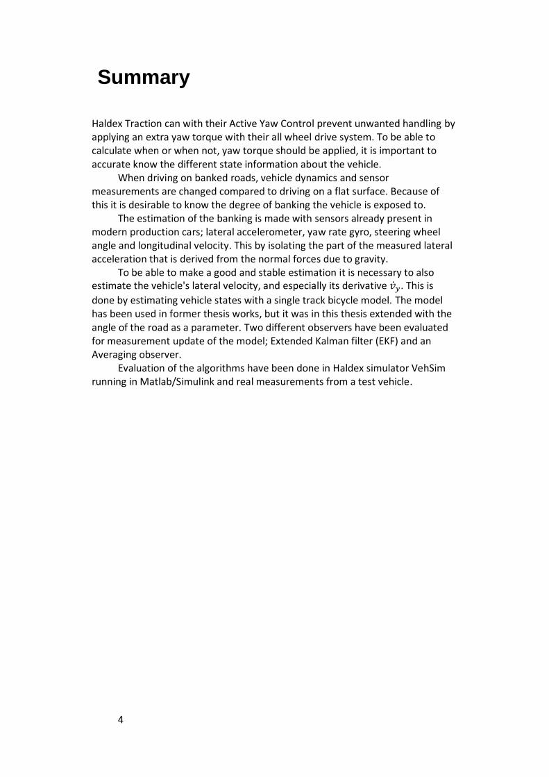
Summary

Haldex Traction can with their Active Yaw Control prevent unwanted handling by applying an extra yaw torque with their all wheel drive system. To be able to calculate when or when not, yaw torque should be applied, it is important to accurate know the different state information about the vehicle.

When driving on banked roads, vehicle dynamics and sensor measurements are changed compared to driving on a flat surface. Because of this it is desirable to know the degree of banking the vehicle is exposed to.

The estimation of the banking is made with sensors already present in modern production cars; lateral accelerometer, yaw rate gyro, steering wheel angle and longitudinal velocity. This by isolating the part of the measured lateral acceleration that is derived from the normal forces due to gravity.

To be able to make a good and stable estimation it is necessary to also estimate the vehicle's lateral velocity, and especially its derivative . This is

done by estimating vehicle states with a single track bicycle model. The model has been used in former thesis works, but it was in this thesis extended with the angle of the road as a parameter. Two different observers have been evaluated for measurement update of the model; Extended Kalman filter (EKF) and an Averaging observer.

Evaluation of the algorithms have been done in Haldex simulator VehSim running in Matlab/Simulink and real measurements from a test vehicle.

5

1. Introduction

For those readers that are new to vehicle dynamics, explanations of certain expressions and physical units can be found in chapter 10.

1.1 Background

Prevention of vehicle accidents is of great interest to all manufacturers today. To prevent accidents it is preferable to predict the vehicles handling and with different systems compensate for unwanted handling and make the car stable. One problem is that vehicle handling is non linear due to tire characteristics, which makes the prediction difficult.

When driving under normal conditions the slip between tire and road is small and the yaw rate is proportional to the steering wheel angle. Then the handling can be assumed to be linear and the behavior can be predicted with high accuracy. When the slip becomes large and the vehicle starts to skid the handling becomes nonlinear and hard to predict.

The Electronic Stability Program (ESP) is a standard safety feature in most cars today. This gives the vehicle the ability to prevent side slip by applying brake force on individual tires. This produces a yaw torque to eliminate the torque produced by the side slip.

The ESP system gets information from the car’s yaw rate sensor, lateral acceleration sensor, wheel speeds and steering wheel angle and uses these parameters to estimate the vehicle behavior. If the estimation shows that the vehicle is becoming unstable or the behavior is unwanted the ESP apply brake force to stabilize the car. This makes the car stable, but the performance is reduced.

Haldex Traction AB has developed a torque biasing device called Haldex Limited Slip Coupling. This device can change the torque applied at the front and rear wheels which gives the ability to also create a yaw torque to counter the torque created by the side slip. When dividing the torque the lateral forces on the rear and front wheels will change thus creating a yaw torque. This gives the advantage of keeping performance and maintaining stability. [1]

The commercial roads today contain a lot of banked curves deliberately created by Trafikverket. This helps rain and water drainage as well as decreases the risk of side slip under bad road conditions such as ice. The banking limit allowed in Sweden is depending on the radius of the curve, speed limit and comfort level, but the maximum allowed is 5.5 percent, which correspond to 3.2 degrees. [8]

6

Since the vehicles sometimes also is driven at raceways, such as Sturup Raceway, larger banking angles is sometimes also present. At Sturup Raceway was the largest banking angle about 10 degrees. Haldex Traction AB has an algorithm for calculating the banking angle today. This needs to be filtered and gives very poor and unreliable results.

Some states needed for the different algorithms in this thesis are immeasurable in normal modern production cars today. Since one of the limitations in this thesis was to only use sensors that are fitted on modern production cars, these states need to be estimated. This is done today by an onboard one track model that simulates the vehicle in real time. The states that are needed can then be extracted from the model. The performance of the model is decided by its complexity. More degrees of freedom and higher complexity with for example dampeners, complete tire model and so on will give better results. The downside with a complex model is that it will need a lot of computing power, which is limited in cars, and tuning. The model can be extended with measured signals which correct the states of the model towards the states of the real vehicle. This addition is called an observer. There are a variety of observers based on different approaches and varying complexity.

1.2 Problem formulation

When driving in banked curves the behavior of a vehicle changes, the steering wheel does not need to be turned as much as for a flat curve with the same radius. This is because the normal force now provides a component that drags the vehicle towards the center of the curve. The lateral acceleration sensor will be affected by a component of gravity. The load distribution on the wheels will also change due to the banking.

Since the onboard model used today do not take the lateral acceleration generated by gravity into consideration, the output from the model and real measurements from the sensor will differ. The yaw rate measurement is normally proportional to the steering angle. But as described above the steering angle is reduced when driving in a banked curve and then the calculated yaw rate will differ from the measured yaw rate. These changes in the vehicle behavior will make the yaw control algorithm detect an error between wanted and estimated behavior and therefore it will compensate by applying brake force to the tires, or applying torque to make the vehicle go in the direction where the wheels are pointing. This means that the vehicle steers out of the curve.

It is important to make clear that this problem isn't specifically a problem in four wheel drive vehicles, but in all vehicles using the same method for predict unwanted handling.

7

1.3 Research objective

The main focus of this thesis will be on finding an algorithm for estimating the banking degree of the road and detection of banked curves. This also includes different filtering algorithms and techniques. It will also include work on updating the existing model with one additional degree of freedom and getting acceptable results on estimation of parameters. Different observers will also be researched and tested on the model. The model should perform well in the linear region of driving and acceptable in the nonlinear range. These changes will help the yaw control of the car function more properly in banked curves.

The algorithm should be robust and yield reliable results and as close to reality as possible with as small delay as possible. Measurement of the banking could be done by a gyro sensor, but it is too expensive and therefore the problem needs to be solved with the sensors and equipment already fitted in a normal vehicle.

The result should be sent to the onboard computer, which will compensate for the banking and make sure the yaw control do not activate in wrong situations and introduce unwanted behavior. Since the onboard computer is limited in its capacity of calculation, this will be a limitation and the algorithm should be as light in computation as possible.

1.4 Related work

For state estimation of vehicles there is much research done. At Haldex Traction AB only, two interesting master theses have been published. These are ‘Design and Validation of a Vehicle State Estimator’ by Schoutissen S.L.G.F., 2004 [10], and ‘Estimation of Vehicle Lateral Velocity’ by Pierre Pettersson, 2008 [9]. The later one by Pierre Petterson includes a two track model. This is needed to model the roll behavior of a car in curves and can also take different load transfers into consideration. For estimation of banking there is not much research done. Some documents from Haldex's own research were received, but these are unfortunately confidential.

8

2. Tools and conditions

To be able to verify and test different algorithms test data are required. All test data were processed in MATLAB/Simulink, but collection of it was made in two different ways.

2.1 MATLAB/Simulink - VehSim

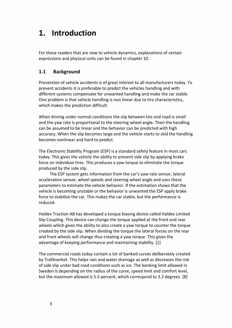
Haldex VehSim is an advanced car simulator built in Simulink for testing and development of software algorithms. Figure 2.1 shows the different high level modules of the simulator.

Figure 2.1 - Haldex VehSim

It is a very complex simulator, which calculates every force acting at every single part that influences the road behavior of the car. The construction of the model is made in such a way as a normal car is constructed. The model has independent modules for each wheel hub, dampeners, gearbox, power train etc.

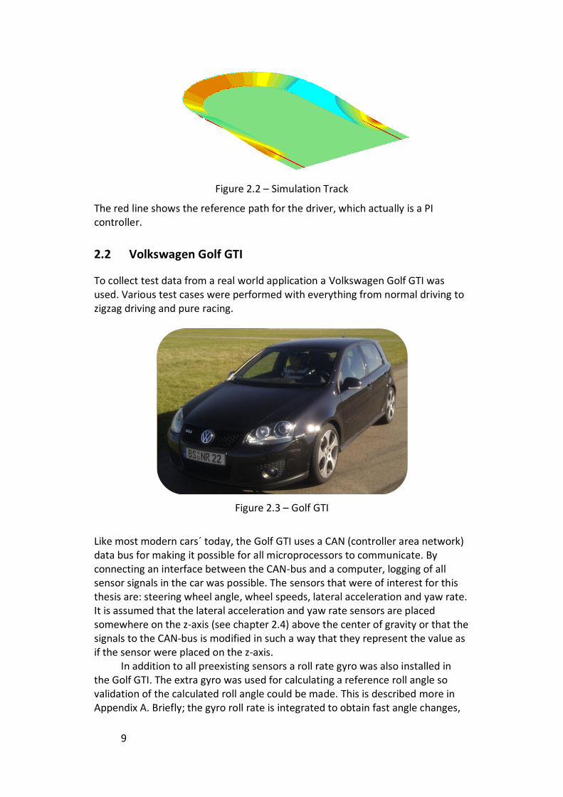
A test track that simulates gravity, air resistance, road friction etc. can be made in different shapes. The most used simulation test track in this thesis is a 180 degree turn with a 20 degree banking angle, as seen in Figure 2.2.

9

Figure 2.2 – Simulation Track

The red line shows the reference path for the driver, which actually is a PI controller.

2.2 Volkswagen Golf GTI

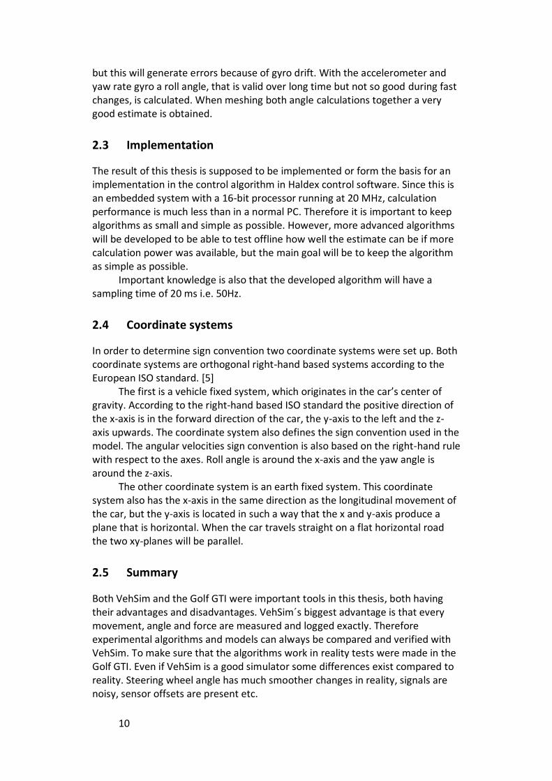
To collect test data from a real world application a Volkswagen Golf GTI was used. Various test cases were performed with everything from normal driving to zigzag driving and pure racing.

Figure 2.3 – Golf GTI

Like most modern cars´ today, the Golf GTI uses a CAN (controller area network) data bus for making it possible for all microprocessors to communicate. By connecting an interface between the CAN-bus and a computer, logging of all sensor signals in the car was possible. The sensors that were of interest for this thesis are: steering wheel angle, wheel speeds, lateral acceleration and yaw rate. It is assumed that the lateral acceleration and yaw rate sensors are placed somewhere on the z-axis (see chapter 2.4) above the center of gravity or that the signals to the CAN-bus is modified in such a way that they represent the value as if the sensor were placed on the z-axis.

In addition to all preexisting sensors a roll rate gyro was also installed in the Golf GTI. The extra gyro was used for calculating a reference roll angle so validation of the calculated roll angle could be made. This is described more in Appendix A. Briefly; the gyro roll rate is integrated to obtain fast angle changes,

10

but this will generate errors because of gyro drift. With the accelerometer and yaw rate gyro a roll angle, that is valid over long time but not so good during fast changes, is calculated. When meshing both angle calculations together a very good estimate is obtained.

2.3 Implementation

The result of this thesis is supposed to be implemented or form the basis for an implementation in the control algorithm in Haldex control software. Since this is an embedded system with a 16-bit processor running at 20 MHz, calculation performance is much less than in a normal PC. Therefore it is important to keep algorithms as small and simple as possible. However, more advanced algorithms will be developed to be able to test offline how well the estimate can be if more calculation power was available, but the main goal will be to keep the algorithm as simple as possible.

Important knowledge is also that the developed algorithm will have a sampling time of 20 ms i.e. 50Hz.

2.4 Coordinate systems

In order to determine sign convention two coordinate systems were set up. Both coordinate systems are orthogonal right-hand based systems according to the European ISO standard. [5]

The first is a vehicle fixed system, which originates in the car’s center of gravity. According to the right-hand based ISO standard the positive direction of the x-axis is in the forward direction of the car, the y-axis to the left and the z-axis upwards. The coordinate system also defines the sign convention used in the model. The angular velocities sign convention is also based on the right-hand rule with respect to the axes. Roll angle is around the x-axis and the yaw angle is around the z-axis.

The other coordinate system is an earth fixed system. This coordinate system also has the x-axis in the same direction as the longitudinal movement of the car, but the y-axis is located in such a way that the x and y-axis produce a plane that is horizontal. When the car travels straight on a flat horizontal road the two xy-planes will be parallel.

2.5 Summary

Both VehSim and the Golf GTI were important tools in this thesis, both having their advantages and disadvantages. VehSim´s biggest advantage is that every movement, angle and force are measured and logged exactly. Therefore experimental algorithms and models can always be compared and verified with VehSim. To make sure that the algorithms work in reality tests were made in the Golf GTI. Even if VehSim is a good simulator some differences exist compared to reality. Steering wheel angle has much smoother changes in reality, signals are noisy, sensor offsets are present etc.

11

3. Theoretical solution

As mentioned earlier Haldex had before the beginning of this thesis work already developed and implemented an algorithm for calculating road banking. It works quite well when driving steady without making any sudden turns, but one of the major problems with this equation was that it incorrectly detected large banking angles when none existed e.g. when driving and side slipping on a frozen lake. Because of this the output of their algorithm is filtered very hard which mean that it is also slow to detect existing road banking angles. Haldex used the following physical equation for calculating roll angle:

[3.1]

and its solution:

[3.2]

where

= roll angle = vehicle longitudinal speed

= vehicle yaw rate = vehicle acceleration in y direction

g = gravitation

It contains all three of the most important units for calculation of road banking angle, which are measurable in today's vehicles: vehicle speed, yaw rate and lateral acceleration. The cosines in 3.1 is an approximation to adjust for the fact of the yaw rate gyro tilt in a banked curve. How this equation is derived is shown in the following part.

3.1 Derivation of the equation for calculating road banking

At first it is important to differentiate between road banking angle and chassis roll angle relative the environment coordinate system. Due to suspension the vehicle chassis will roll relative to the road ) when exposed to lateral forces. Because of all sensors being placed in the chassis it is also the chassis roll that can be indirectly measured. To achieve the exact road banking angle, calculation of vehicle chassis roll relative road is necessary. This will be discussed further in later chapters, but as a starting point will be neglected i.e.

12

and both the vehicle roll angle and the road banking angle will be denoted .

3.1.1 Normal forces due to gravity

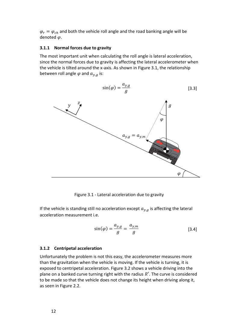
The most important unit when calculating the roll angle is lateral acceleration, since the normal forces due to gravity is affecting the lateral accelerometer when the vehicle is tilted around the x-axis. As shown in Figure 3.1, the relationship between roll angle and is:

[3.3]

Figure 3.1 - Lateral acceleration due to gravity

If the vehicle is standing still no acceleration except is affecting the lateral

acceleration measurement i.e.

[3.4]

3.1.2 Centripetal acceleration

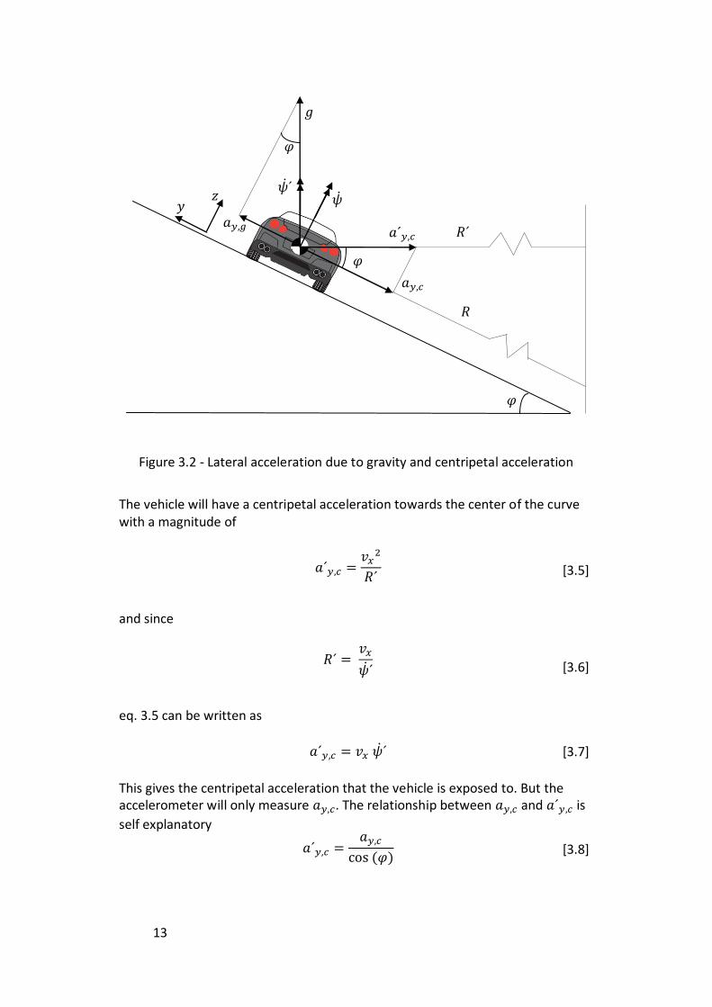
Unfortunately the problem is not this easy, the accelerometer measures more than the gravitation when the vehicle is moving. If the vehicle is turning, it is exposed to centripetal acceleration. Figure 3.2 shows a vehicle driving into the plane on a banked curve turning right with the radius . The curve is considered to be made so that the vehicle does not change its height when driving along it, as seen in Figure 2.2.

13

Figure 3.2 - Lateral acceleration due to gravity and centripetal acceleration

The vehicle will have a centripetal acceleration towards the center of the curve with a magnitude of

[3.5]

and since

[3.6]

eq. 3.5 can be written as

[3.7]

This gives the centripetal acceleration that the vehicle is exposed to. But the accelerometer will only measure . The relationship between and is

self explanatory

[3.8]

14

But the relationship between and has to be proven further. It is also at this point our and Haldex equation will differ. With the knowledge that

[3.9]

together with equation 3.6 we get

[3.10]

and with eq. 3.7 this gives

[3.11]

With this knowledge equation 3.4 now extends to

[3.12]

This result is the same as the one by Haldex except of the cosine function. In equation 3.1 the centripetal acceleration is measured in the environment's coordinate system, but since the vehicle always measure in its own coordinate system this will generate an error that depends on the roll angle. A positive coincidence of equation 3.12 is the fact that its solution is considerably shorter and simpler in terms of computation. Validation of the equation was made in Haldex VehSim. Figure 2.2 shows how the virtual test track with a 20 degree banking was built. The test vehicle starts at the left straight part facing the curve, at 18 m/s. Then a virtual driver, written as a PI regulator, drives through the curve trying to follow the middle. Figure 3.3 shows a comparison between equation 3.1 and 3.12 when both are using the same exact signals.

15

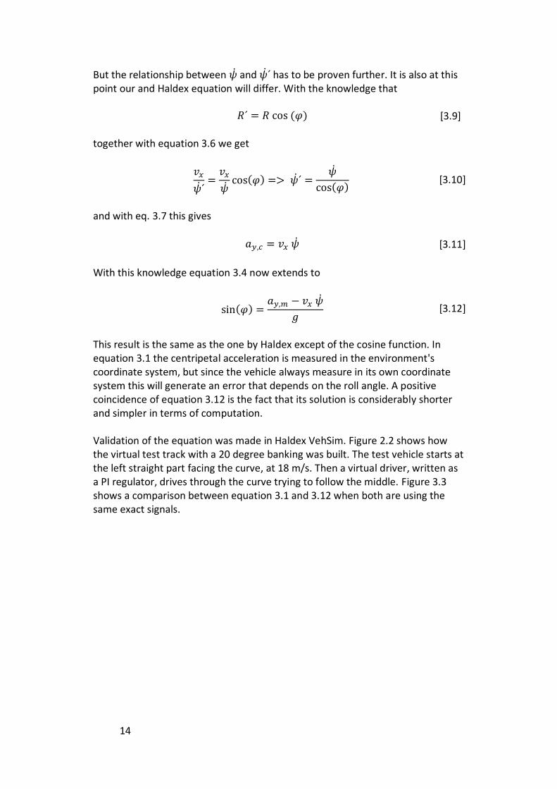
Figure 3.3 - Comparison between eq. 3.1 and 3.12

The driver reaches the curve at approx. 7,5 seconds and is then making a very sudden turn and is driving out of the curve at approx. 19 seconds after start. As seen, the different equations correlate well when the yaw rate and roll angle is zero. But when driving in the banked curve 3.1 deviates from the correct angle because of its extra cosine function. By this example it is shown that equation 3.12 correlates better to the reference roll angle then 3.1.

The sudden deviations from the correct angle, especially in the beginning and end of the curve were at first the main problem. These correlated well with a high derivative of the steering angle. So by using the steering angle a good filter could be made that filtered these sudden changes, and a decent result was obtained.

3.1.3 Lateral velocity derivative

A vehicle do not only have a longitudinal velocity, but also a lateral velocity ( ).

It is often very small, but exists when turning due to lateral slip. Changes in lateral velocity are producing a lateral acceleration . The formula was extended

so that influences from also was removed from the measured acceleration.

[3.13]

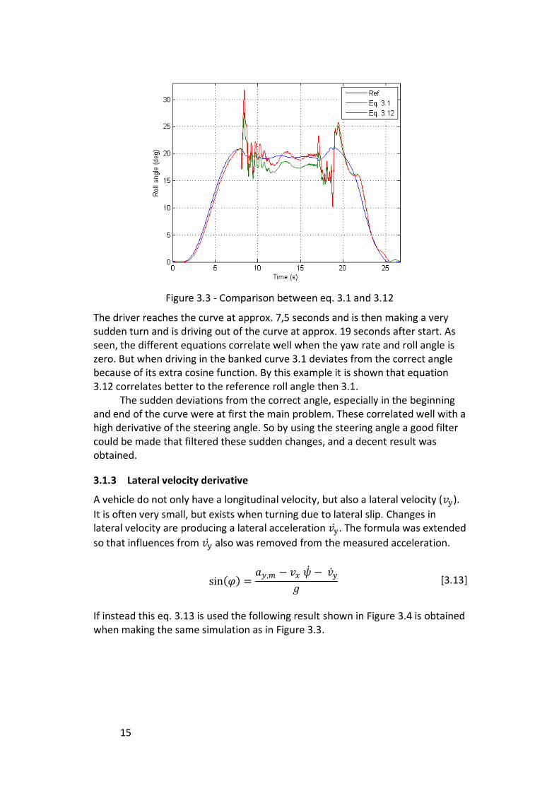
If instead this eq. 3.13 is used the following result shown in Figure 3.4 is obtained when making the same simulation as in Figure 3.3.

16

Figure 3.4 - Eq. 3.13

With this result it is stated that equation 3.13 correlates much better since the part much reduces the transient errors. Since lateral acceleration,

longitudinal velocity and yaw rate all are measured in modern vehicles, 3 out of 4 units are already is known. The problem is to maintain an acceptable , which

has to be estimated.

3.1.4 Limitation

Equation 3.13 works well when small or no lateral slip is present, but if greater lateral slip occurs problems arise. If the rear tires for instance is slipping much but the front tires are not, this will generate a yaw rate. This yaw rate will in the formula appear as a contribution to the centripetal force which is not present because the car is actually slipping. More information about how to handle this problem and how it affects the formula and model will be discussed later when more knowledge about vehicle dynamics is explained.

17

4. Modeling

4.1 Vehicle modeling overview

To describe the car dynamics the essential variables are yaw rate, longitudinal – and lateral velocity. The model on the other hand can be done in several different ways. Problems that can occur with a complicated model with a lot of different parameters are that if any parts are changed on the car the model will contain errors due to the configuration of the old parameters for the old part. Therefore it would be preferable to combine as much of the different parameters in one single simplified parameter. This would also ease the work of tuning the model to match the car characteristics.

Since the car has limited computing capacity the model must be kept simple but still capture the essential dynamics of the car. The model used in this thesis will be a one track model. The one track model is based on a bicycle and has four degrees of freedom; longitudinal- and lateral velocity, yaw rate, roll angle.

The model consists of two main parts, the tire model and chassis model. These are linked together in such way that the tire forces affect the chassis movement.

4.2 Bicycle model

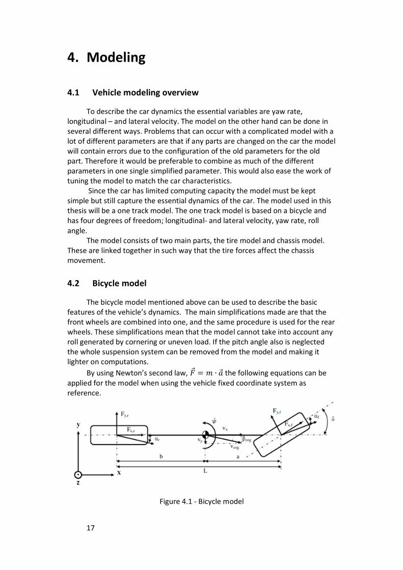
The bicycle model mentioned above can be used to describe the basic features of the vehicle’s dynamics. The main simplifications made are that the front wheels are combined into one, and the same procedure is used for the rear wheels. These simplifications mean that the model cannot take into account any roll generated by cornering or uneven load. If the pitch angle also is neglected the whole suspension system can be removed from the model and making it lighter on computations.

By using Newton’s second law, the following equations can be applied for the model when using the vehicle fixed coordinate system as reference.

Figure 4.1 - Bicycle model

18

[4.1]

[4.2]

The force on the vehicle created by the centripetal acceleration:

[4.3]

When combining equations [4.1], [4.2] and [4.3] the result is:

[4.4]

The torque around the z-axis

[4.5]

where m is representing the mass of the car, the lateral velocity, the

longitudinal velocity, the moment of inertia, a and b the length from the center of gravity to the front and rear axles, the front wheel angle and the roll angel with respect to the horizontal plane. The tire forces are essential to estimate correctly in order to obtain a functional model. To estimate these forces it is crucial to calculate acceptable slip angles. In this case the longitudinal tire forces are assumed to be small with respect to the lateral forces and therefore the lateral forces almost only depend on the slip angle.

For the bicycle model the equations for the slip angle become: [1]

[4.6]

[4.7]

4.3 Tire model

When building a model for estimation of vehicle states the tire is the most central part. Except air resistance and of course gravity, friction due to ground contact is the only external force acting on the vehicle. At the same time it is

19

probably the most difficult part to model. Very much research has been made within this area and several papers and books have been published, but still no one has invented a perfect model of the tire, even if there exists very complex and nearly perfect models.

Because of limited calculation power we will use as simple model as possible as long as the result is satisfying. Another reason for not using a too complex model is the lack of scientific data of the tires and with increasing number of parameters it gets harder to tune the model. Even with plenty of scientific data a too complex model would be unnecessary because of the fact that tires changes their properties over time and in many countries different types of tires are used depending on the season.

The main focus when modeling a tire is to attain the lateral force . In the three different tire models used in this work is calculated as a function of the slip angle .

4.3.1 Magic Formula

A commonly used and effective model of the tire forces is the Magic Formula. It was presented by Hans B. Pacejka and its name comes from the reason that it was not developed from physical properties. Instead a formula was developed that was consistent with the test data. It has been proven to be a good estimation of the tire.

The expression gives the relationship between lateral tire force and slip angle:

[4.8]

where

stiffness factor

peak factor

cornering stiffness

, shape factors maximum cornering stiffness load at maximum cornering stiffness

4.3.2 Exponential tire model

A simpler model that captures the main characteristics of the tire is the exponential tire model:

20

[4.9]

It results in lighter computations and the parameter is the only parameter that needs to be tuned.

21

4.3.3 Linear tire model

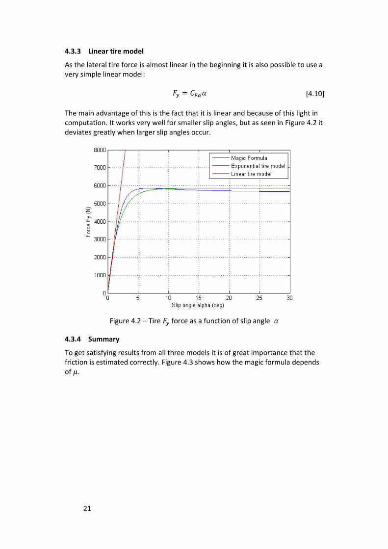
As the lateral tire force is almost linear in the beginning it is also possible to use a very simple linear model:

[4.10]

The main advantage of this is the fact that it is linear and because of this light in computation. It works very well for smaller slip angles, but as seen in Figure 4.2 it deviates greatly when larger slip angles occur.

Figure 4.2 – Tire force as a function of slip angle

4.3.4 Summary

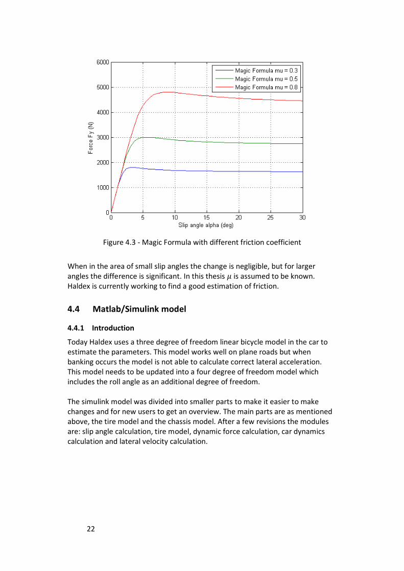
To get satisfying results from all three models it is of great importance that the friction is estimated correctly. Figure 4.3 shows how the magic formula depends of .

22

Figure 4.3 - Magic Formula with different friction coefficient

When in the area of small slip angles the change is negligible, but for larger angles the difference is significant. In this thesis is assumed to be known. Haldex is currently working to find a good estimation of friction.

4.4 Matlab/Simulink model

4.4.1 Introduction

Today Haldex uses a three degree of freedom linear bicycle model in the car to estimate the parameters. This model works well on plane roads but when banking occurs the model is not able to calculate correct lateral acceleration. This model needs to be updated into a four degree of freedom model which includes the roll angle as an additional degree of freedom.

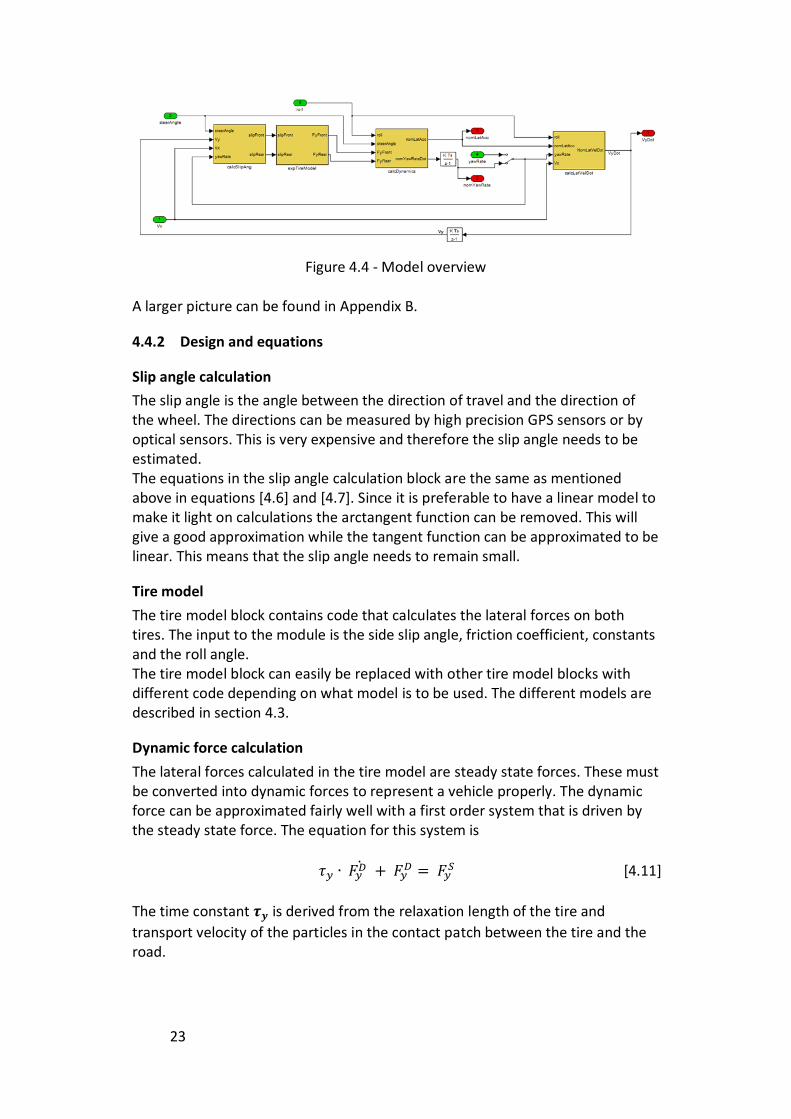
The simulink model was divided into smaller parts to make it easier to make changes and for new users to get an overview. The main parts are as mentioned above, the tire model and the chassis model. After a few revisions the modules are: slip angle calculation, tire model, dynamic force calculation, car dynamics calculation and lateral velocity calculation.

23

Figure 4.4 - Model overview

A larger picture can be found in Appendix B.

4.4.2 Design and equations

Slip angle calculation

The slip angle is the angle between the direction of travel and the direction of the wheel. The directions can be measured by high precision GPS sensors or by optical sensors. This is very expensive and therefore the slip angle needs to be estimated. The equations in the slip angle calculation block are the same as mentioned above in equations [4.6] and [4.7]. Since it is preferable to have a linear model to make it light on calculations the arctangent function can be removed. This will give a good approximation while the tangent function can be approximated to be linear. This means that the slip angle needs to remain small.

Tire model

The tire model block contains code that calculates the lateral forces on both tires. The input to the module is the side slip angle, friction coefficient, constants and the roll angle. The tire model block can easily be replaced with other tire model blocks with different code depending on what model is to be used. The different models are described in section 4.3.

Dynamic force calculation

The lateral forces calculated in the tire model are steady state forces. These must be converted into dynamic forces to represent a vehicle properly. The dynamic force can be approximated fairly well with a first order system that is driven by the steady state force. The equation for this system is

[4.11]

The time constant is derived from the relaxation length of the tire and

transport velocity of the particles in the contact patch between the tire and the road.

24

[4.12]

Where represents the tire’s relaxation length, the angular velocity of the

wheel and the tire’s radius. The relaxation length is a function of the longitudinal and lateral slip, and

the wheel load. If the relaxation length is set to a constant it will only approximate the real tire behavior in a zero order system. [4]

Because of this fact, relaxation length is not used in our models.

Car dynamics calculations

In the car dynamics calculation box the equilibrium equations stated above are used and rewritten. The output of the module is the lateral acceleration and the acceleration around the car’s z-axis. The lateral acceleration is calculated in such way that it should approximate the measured value from the sensor. The forces acting on the car in the lateral direction is obviously the lateral forces from the tires. These are divided by the car´s mass to get acceleration according to Newton.

[4.13]

The acceleration around the z-axis is calculated in such way that the lateral forces from the tires multiplied with the length to the center of gravity creates a resulting torque on the car. This divided by the inertia around the z-axis will then be the angle acceleration around the z-axis.

[4.14]

The acceleration around the z-axis is then integrated to get the angle velocity,

also denoted as the yaw rate ( ).

Lateral velocity calculation

The lateral velocity is an important parameter and a proper approximation is essential. Many theses has been written about estimation of the lateral velocity and its importance in car modeling. In this thesis the equation used for calculation of the lateral velocity in the model is:

[4.15]

is then integrated to get the velocity. The problem with integrating an

unstable signal is that errors will accumulate and become larger and larger. Therefore it is important to estimate as accurately as possible.

25

4.4.3 Results

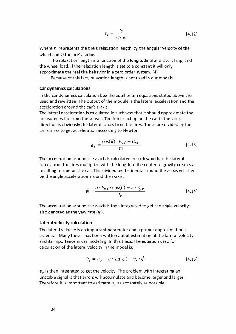
While driving under normal circumstances the model performs very well and gives close to perfect results on the lateral acceleration and yaw rate calculations. The problem is to calculate the lateral velocity. The result is acceptable but not as good as the rest. The problem with the model is that it does not handle the change of the load transfer. To do this a two track model needs to be used, like in Pettersson’s thesis, [9]. This though is much more computationally heavy. In the simulation below the nonlinear model uses the nonlinear slip angle calculations from equations 4.6 and 4.7, and the exponential tire model with tuned parameters described in 4.3.2. The linear model uses the modified slip angle calculations without the arctangent function and the linear tire model described in 4.3.3. Both models have the same input signals, longitudinal velocity, steering angle and the true banking angle of the chassis calculated by VehSim. The true value is the value presented by Haldex VehSim.

Normal driving in curve with radius 60m

Figure 4.5 - Chassis roll angle when driving in curve without banking

26

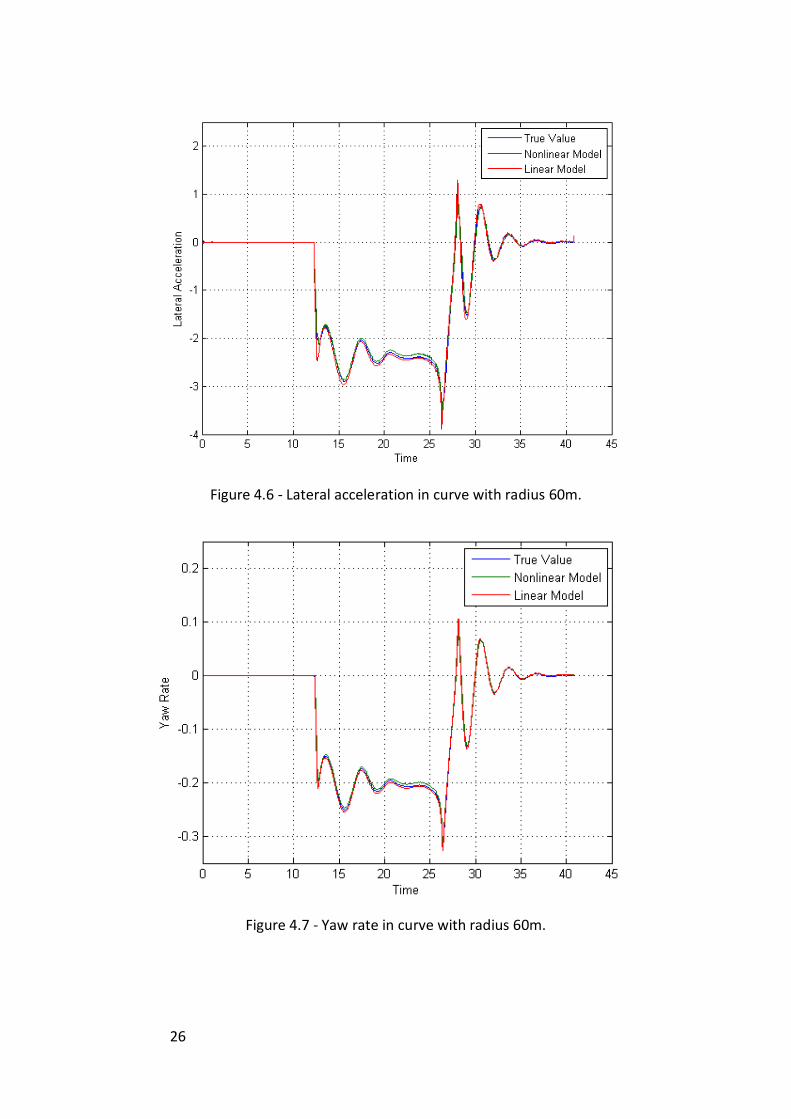
Figure 4.6 - Lateral acceleration in curve with radius 60m.

Figure 4.7 - Yaw rate in curve with radius 60m.

27

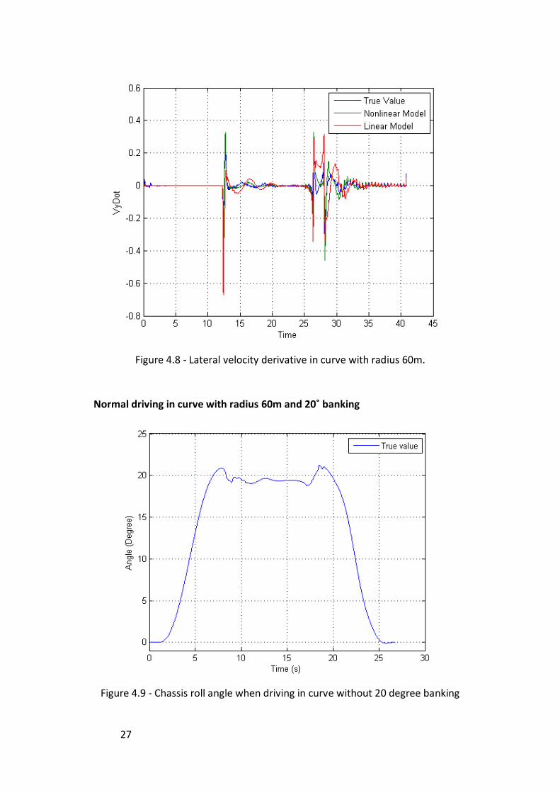
Figure 4.8 - Lateral velocity derivative in curve with radius 60m.

Normal driving in curve with radius 60m and 20˚ banking

Figure 4.9 - Chassis roll angle when driving in curve without 20 degree banking

28

Figure 4.10 - Lateral acceleration in curve with radius 60m and 20˚ banking

Figure 4.11 - Yaw rate in curve with radius 60m and 20˚ banking

29

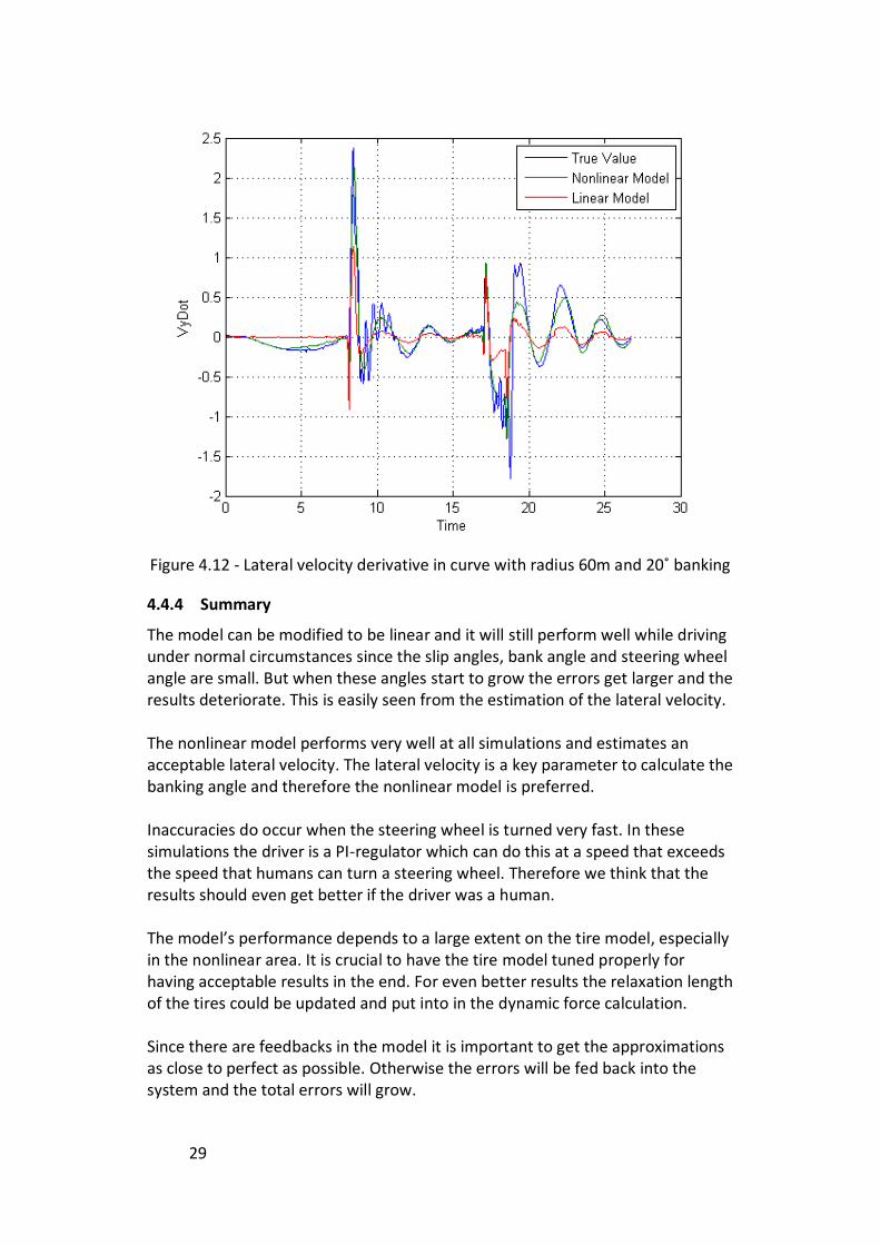
Figure 4.12 - Lateral velocity derivative in curve with radius 60m and 20˚ banking

4.4.4 Summary

The model can be modified to be linear and it will still perform well while driving under normal circumstances since the slip angles, bank angle and steering wheel angle are small. But when these angles start to grow the errors get larger and the results deteriorate. This is easily seen from the estimation of the lateral velocity. The nonlinear model performs very well at all simulations and estimates an acceptable lateral velocity. The lateral velocity is a key parameter to calculate the banking angle and therefore the nonlinear model is preferred. Inaccuracies do occur when the steering wheel is turned very fast. In these simulations the driver is a PI-regulator which can do this at a speed that exceeds the speed that humans can turn a steering wheel. Therefore we think that the results should even get better if the driver was a human. The model’s performance depends to a large extent on the tire model, especially in the nonlinear area. It is crucial to have the tire model tuned properly for having acceptable results in the end. For even better results the relaxation length of the tires could be updated and put into in the dynamic force calculation. Since there are feedbacks in the model it is important to get the approximations as close to perfect as possible. Otherwise the errors will be fed back into the system and the total errors will grow.

30

5. Observer techniques

5.1 Overview

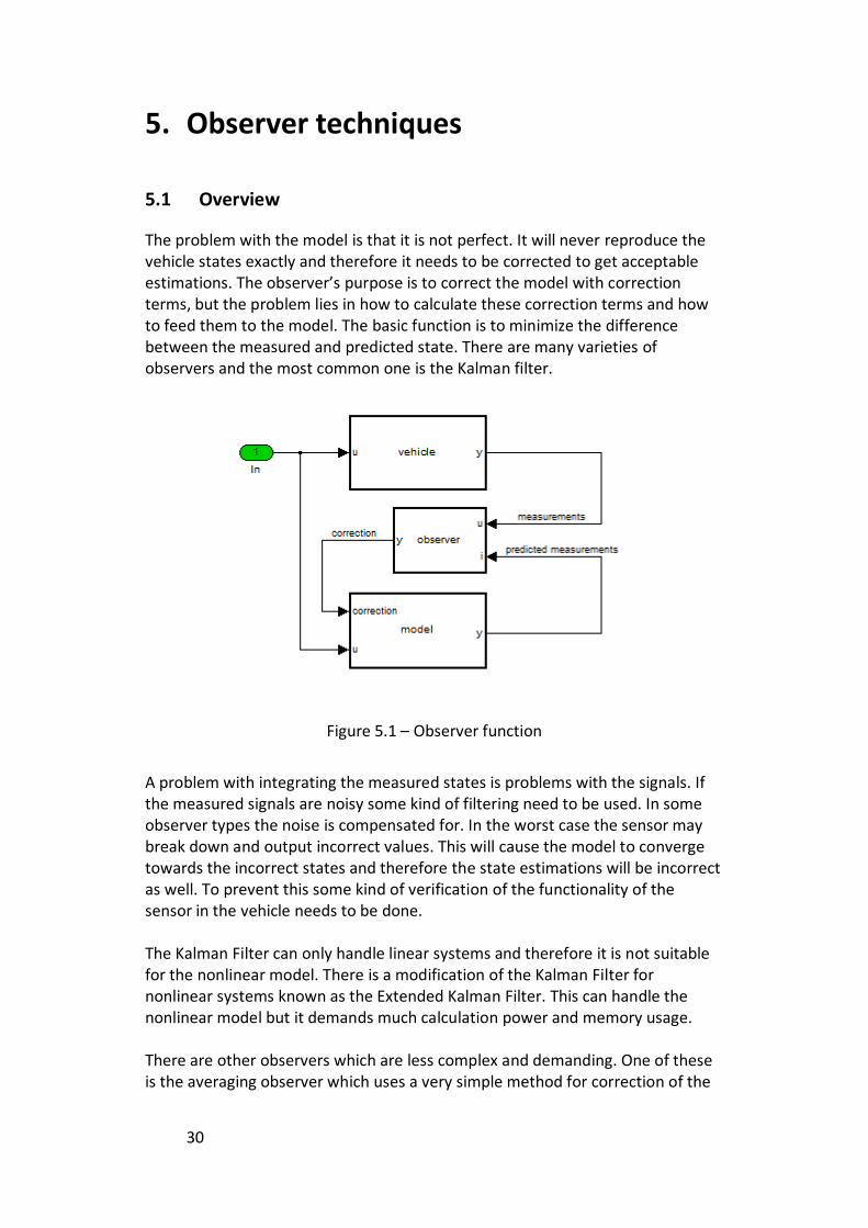
The problem with the model is that it is not perfect. It will never reproduce the vehicle states exactly and therefore it needs to be corrected to get acceptable estimations. The observer’s purpose is to correct the model with correction terms, but the problem lies in how to calculate these correction terms and how to feed them to the model. The basic function is to minimize the difference between the measured and predicted state. There are many varieties of observers and the most common one is the Kalman filter.

Figure 5.1 – Observer function

A problem with integrating the measured states is problems with the signals. If the measured signals are noisy some kind of filtering need to be used. In some observer types the noise is compensated for. In the worst case the sensor may break down and output incorrect values. This will cause the model to converge towards the incorrect states and therefore the state estimations will be incorrect as well. To prevent this some kind of verification of the functionality of the sensor in the vehicle needs to be done. The Kalman Filter can only handle linear systems and therefore it is not suitable for the nonlinear model. There is a modification of the Kalman Filter for nonlinear systems known as the Extended Kalman Filter. This can handle the nonlinear model but it demands much calculation power and memory usage. There are other observers which are less complex and demanding. One of these is the averaging observer which uses a very simple method for correction of the

31

model. These different observers will be tested and compared to see how much performance you can trade off for complexity and demands.

5.2 Averaging observer

The averaging observer uses the assumption that the true state value must be positioned somewhere between the measured and predicted state value. The measured and predicted state value is then weighted depending on which is closest to the true state value and the average value is calculated.

The average observer resembles a standard P-regulator with the weight function as the gain. The main disadvantage with the P-regulator is steady state errors and that it never reaches its target value. This can be handled with an introduction of an integration part to the controller.

where is the parameter for how much the models state values should be used, is the parameter for how much the measured state values should be used, is the parameter for the integral part. This should be kept as close to zero as possible to ensure stability. For noisy and unreliable measurements the model should be weighted higher than the measurements and then . In the nonlinear area of the behavior the measurements should be weighted higher and thus . If the measured value is weighted too low the model will not converge towards the true value which often is closer to the measured value. This demands good measurement signals and therefore they might need some filtering. The advantages of the average observer are the modest calculation power and memory usage, and the tuning is very easy and straight forward.

5.3 Linear Kalman filter

A very well used filter in digital computing is the Kalman filter. It was introduce 1960 by R. E. Kalman [2] and contains mathematical equations that estimate the state of a process in the past, present and future. The estimation is done so the mean of the square error is minimized.

32

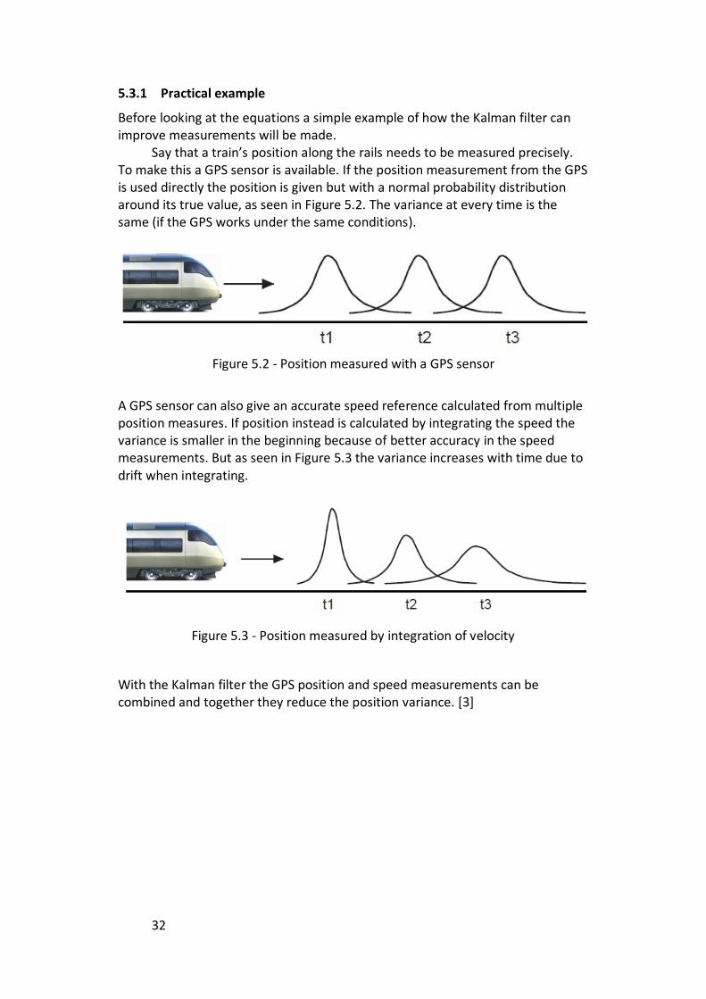
5.3.1 Practical example

Before looking at the equations a simple example of how the Kalman filter can improve measurements will be made.

Say that a train’s position along the rails needs to be measured precisely. To make this a GPS sensor is available. If the position measurement from the GPS is used directly the position is given but with a normal probability distribution around its true value, as seen in Figure 5.2. The variance at every time is the same (if the GPS works under the same conditions).

Figure 5.2 - Position measured with a GPS sensor

A GPS sensor can also give an accurate speed reference calculated from multiple position measures. If position instead is calculated by integrating the speed the variance is smaller in the beginning because of better accuracy in the speed measurements. But as seen in Figure 5.3 the variance increases with time due to drift when integrating.

Figure 5.3 - Position measured by integration of velocity

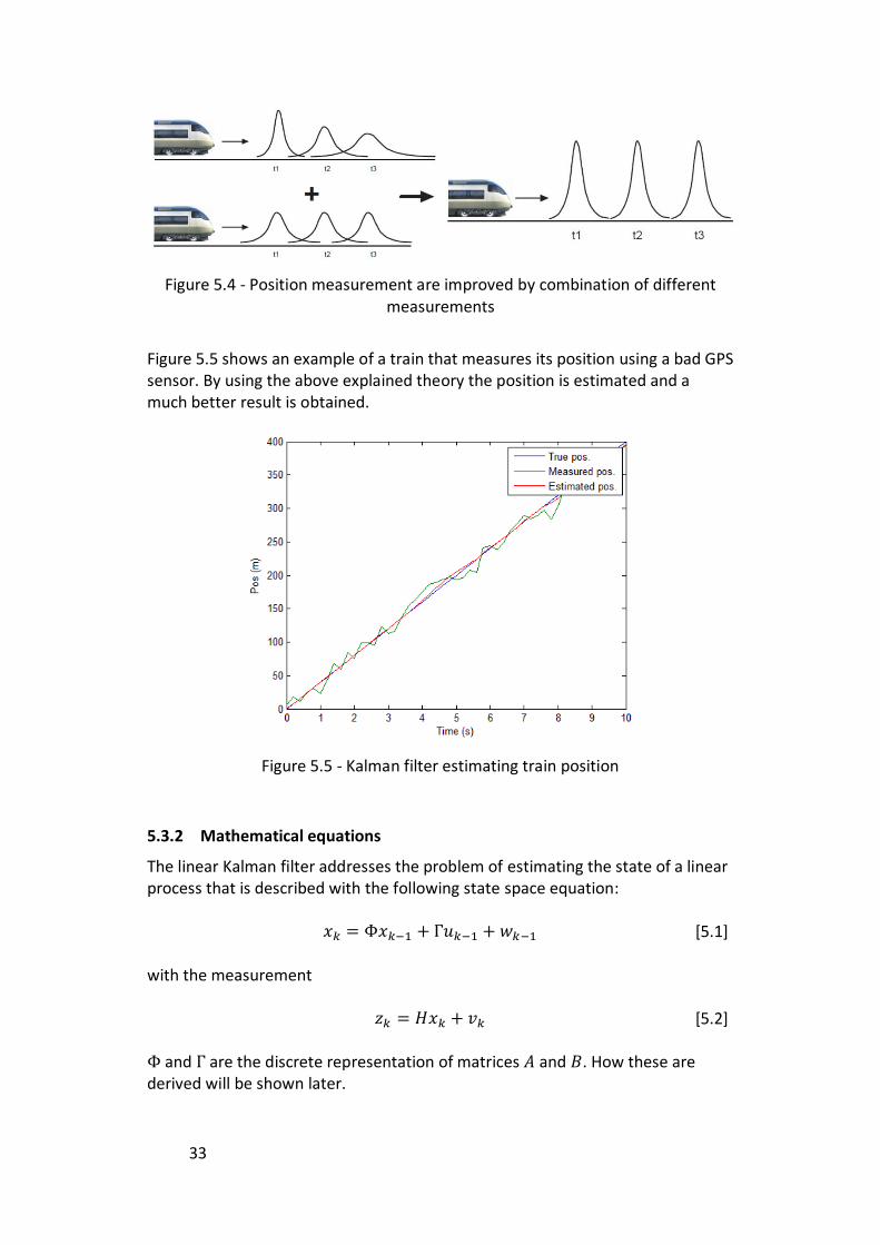
With the Kalman filter the GPS position and speed measurements can be combined and together they reduce the position variance. [3]

33

Figure 5.4 - Position measurement are improved by combination of different measurements

Figure 5.5 shows an example of a train that measures its position using a bad GPS sensor. By using the above explained theory the position is estimated and a much better result is obtained.

Figure 5.5 - Kalman filter estimating train position

5.3.2 Mathematical equations

The linear Kalman filter addresses the problem of estimating the state of a linear process that is described with the following state space equation:

[5.1]

with the measurement

[5.2] and are the discrete representation of matrices and . How these are derived will be shown later.

34

The random variables and , respectively, represent the measurement and process noise. They are assumed to be independent of each other, white noise and with a normal probability distribution.

[5.3]

[5.4] The Kalman filter equations are divided into two groups and are stated as follow: Time update (“predict”)

[5.5]

[5.6] Measurement update (“correct”)

[5.7]

[5.8]

[5.9]

They are linked together as

Figure 5.6 - Kalman filter cycle

is the a priori state estimate based on knowledge of the state prior to

k.

is the a posteriori state estimate at step k based on measurement .

is the true state at step k.

The a priori and a posteriori estimate errors are then defined as

[5.10]

[5.11] which gives a priori and a posteriori estimate error covariances

[5.12]

[5.13]

35

The time update equation uses the state space model to predict future states (a priori), and also predicts the future error covariance. They can be seen as the predictor equations.

To make sure the model does not drift away from the true states, feedback in the form of noisy measurements are updating the model during measurement update. The difference

is called the measurement innovation or the residual and is a measure of how well the model is predicting the state compared to real measurements.

The Kalman gain matrix is the central part of the whole filter. It decides how much of the residual value to be used when updating . A high makes the filter trust the measurements more. In this thesis it is calculated from [5.7], but other equations exist.

As said is a measure of the estimation error, with higher

the Kalman gain also gets higher. So with high values of , the measurements are trusted more, but with high values of measurements are trusted less. [2]

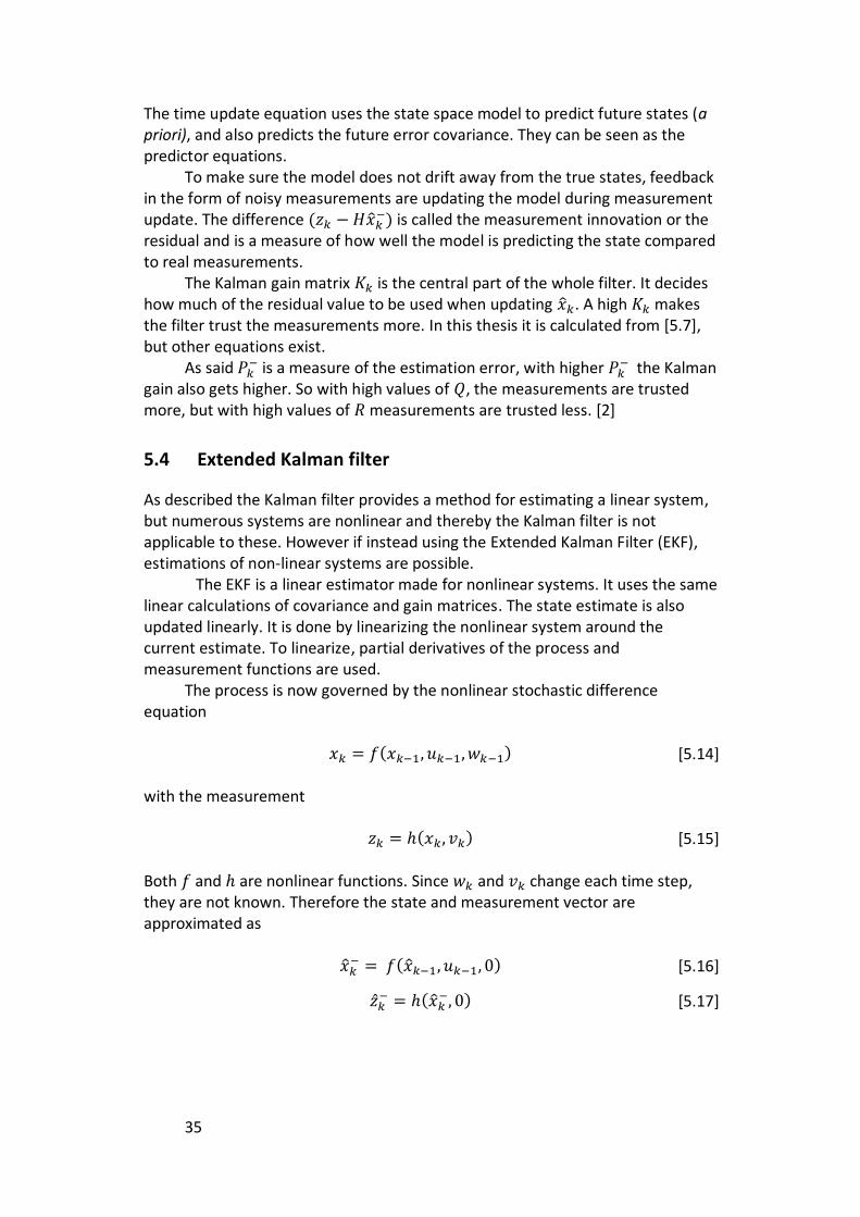
5.4 Extended Kalman filter

As described the Kalman filter provides a method for estimating a linear system, but numerous systems are nonlinear and thereby the Kalman filter is not applicable to these. However if instead using the Extended Kalman Filter (EKF), estimations of non-linear systems are possible. The EKF is a linear estimator made for nonlinear systems. It uses the same linear calculations of covariance and gain matrices. The state estimate is also updated linearly. It is done by linearizing the nonlinear system around the current estimate. To linearize, partial derivatives of the process and measurement functions are used.

The process is now governed by the nonlinear stochastic difference equation

[5.14]

with the measurement

[5.15] Both and are nonlinear functions. Since and change each time step, they are not known. Therefore the state and measurement vector are approximated as

[5.16]

[5.17]

36

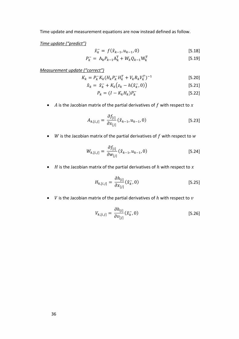
Time update and measurement equations are now instead defined as follow. Time update (“predict”)

[5.18]

[5.19]

Measurement update (“correct”)

[5.20]

[5.21]

[5.22]

is the Jacobian matrix of the partial derivatives of with respect to

[5.23]

is the Jacobian matrix of the partial derivatives of with respect to

[5.24]

is the Jacobian matrix of the partial derivatives of with respect to

[5.25]

is the Jacobian matrix of the partial derivatives of with respect to

[5.26]

37

6. Observer design

6.1 Discretization

Since the algorithm will be implemented in a microprocessor all available signals will be discretized. The conversion from analog to digital is made by holding the analog value one sampling period until the next value is read. This is called Zero-order Hold sampling because of the zero order polynomial between the sampling points.

As signals are processed in discrete time it is also necessary to convert system models from continuous time to discrete. The continuous time system described in statespace form

[6.1]

is converted to its discrete equivalent

[6.2]

with a sampling period of . and is defined as follow

[6.3]

[6.4]

Computation of and can be made in many different ways. Equation [6.3] gives exact values, but in this thesis the following approximation is used to be able to calculate and numerically

[6.5]

[6.6]

[6.7] [6] Numerical integration can be performed in different ways with different stability properties. Common methods are the forward difference, backward difference and Trapezoidal

38

Forward difference (Explicit Euler)

[6.8] Backward difference (Implicit Euler)

[6.9] Trapezoidal (Tustin)

[6.10]

Figure 6.1 – Illustration of integration methods forward difference, backward difference and trapezoidal.

When numerically integrating using these different methods, stability of the system is changed. Figure 6.2 show how a stable continuous system in the s-plane is mapped into the discrete z-plane.

Figure 6.2 - How a continuous system is mapped into the discrete z-plane

Stability in the z-plane is inside the unit circle. In other words can a stable system be mapped into an unstable with forward difference. However if using backward difference all stable continuous system will be stable in the z-plane, but also some unstable ones, which is not desirable. The most used method is the trapezoidal because of its ability to preserve stability conditions. A stable continuous system is mapped into a stable discrete system and vice versa.

Forward difference Backward difference Trapezoidal

39

6.2 Extended Kalman filter

An EKF filter requires much calculation power and is not likely to be implemented in the existing platform. The reason for testing this anyway is to see if the algorithm can be much improved by making more calculations. Another reason is that calculation power in future products probably will increase. The formulas that will be used is:

[6.11]

[6.12]

Lateral tire forces is calculated with the exponential tire formula

and the slip angles are calculated from

To make equations 6.11 and 6.12 take into account of road banking, lateral forces are calculated as

[6.16]

Now the EKF can be assembled. Equations 6.11 and 6.12 are converted into the nonlinear state space so it can be applied to

where

[6.13]

[6.14]

[6.15]

[6.17]

[6.18]

[6.19]

40

The nonlinear functions then become:

[6.20]

From equation 6.20 filter parameters can be calculated. The Jacobian matrix A is derived as follow:

[6.22]

[6.23]

[6.24]

[6.25]

[6.26]

[6.27]

[6.28]

[6.29]

[6.21]

41

Since the yaw rate sensor is measuring the yaw rate directly it is also very precise except of some small noise. This is the most important measurement for updating the model. When only using the yaw rate the measurement vector becomes

[6.30]

which gives the following

If estimation of the road banking angle can be made with good results, can be

calculated by integrating

[6.32]

If some of the parameters has the slightest error this will increase due to integration. Also temperature can cause drift in the accelerometer and make the offset grow. This makes updates using difficult and more of a source to errors

then actually improving the model.

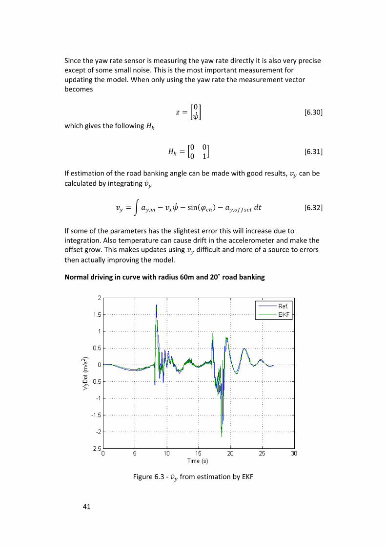
Normal driving in curve with radius 60m and 20˚ road banking

Figure 6.3 - from estimation by EKF

[6.31]

42

Figure 6.3 shows estimated using steering wheel angle, longitudinal velocity

and road banking as system inputs and yaw rate as only updated estimation parameter. Input parameters are exact without any noise.

6.3 Summary

Many tests and configurations were performed on both the averaging observer and the EKF filter. Measurements of the error compared to the reference value together with visual evaluation was made. They both performed well when updating the model with the measured yaw rate. Common for them both were that they both performed better when trusting the measured yaw rate more.

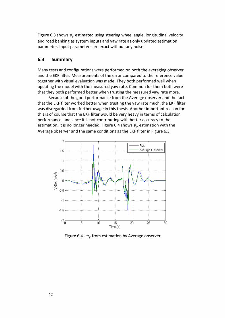
Because of the good performance from the Average observer and the fact that the EKF filter worked better when trusting the yaw rate much, the EKF filter was disregarded from further usage in this thesis. Another important reason for this is of course that the EKF filter would be very heavy in terms of calculation performance, and since it is not contributing with better accuracy to the estimation, it is no longer needed. Figure 6.4 shows estimation with the

Average observer and the same conditions as the EKF filter in Figure 6.3

Figure 6.4 - from estimation by Average observer

43

7. Signal processing and error detection

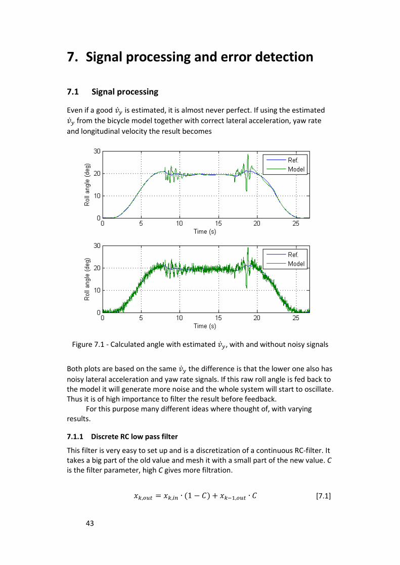
7.1 Signal processing

Even if a good is estimated, it is almost never perfect. If using the estimated

from the bicycle model together with correct lateral acceleration, yaw rate

and longitudinal velocity the result becomes

Figure 7.1 - Calculated angle with estimated , with and without noisy signals

Both plots are based on the same the difference is that the lower one also has

noisy lateral acceleration and yaw rate signals. If this raw roll angle is fed back to the model it will generate more noise and the whole system will start to oscillate. Thus it is of high importance to filter the result before feedback.

For this purpose many different ideas where thought of, with varying results.

7.1.1 Discrete RC low pass filter

This filter is very easy to set up and is a discretization of a continuous RC-filter. It takes a big part of the old value and mesh it with a small part of the new value. C is the filter parameter, high C gives more filtration.

[7.1]

44

Benefits with this are that only one parameter needs to be adjusted, it is very light in computation and only one value needs to be saved between the iterations. On the negative side is the fact that if a high filtration is made it is also slow.

7.1.2 Moving average filter

The moving average filter is a simple form of the FIR-filter. It stores a pre set number of values and calculates the average of them.

Summation of all values is not needed since all values are weighted equally, subtraction of the last one and summation with the new value is only needed. But n values need to be stored.

7.1.3 Discrete RC low pass filter with integral part

Both the discrete low pass filter and the moving average filter introduce a delay when strong filtration is made. By applying an integral part to the RC filter, strong filtration can be made and the signal is still fast over longer time periods. The signal is filtered with equation 7.1 and then the delay error between the filtered and input signal is integrated each time step.

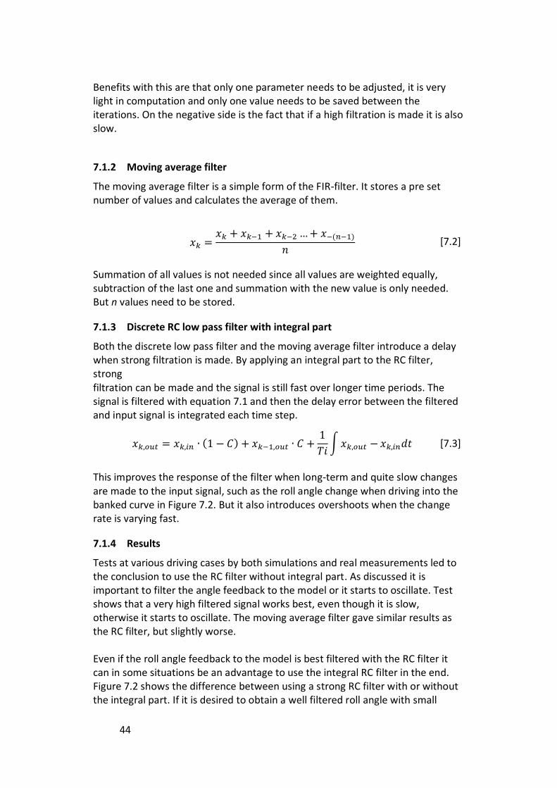
This improves the response of the filter when long-term and quite slow changes are made to the input signal, such as the roll angle change when driving into the banked curve in Figure 7.2. But it also introduces overshoots when the change rate is varying fast.

7.1.4 Results

Tests at various driving cases by both simulations and real measurements led to the conclusion to use the RC filter without integral part. As discussed it is important to filter the angle feedback to the model or it starts to oscillate. Test shows that a very high filtered signal works best, even though it is slow, otherwise it starts to oscillate. The moving average filter gave similar results as the RC filter, but slightly worse. Even if the roll angle feedback to the model is best filtered with the RC filter it can in some situations be an advantage to use the integral RC filter in the end. Figure 7.2 shows the difference between using a strong RC filter with or without the integral part. If it is desired to obtain a well filtered roll angle with small

[7.2]

[7.3]

45

delays during big roll angle changes as in the figure the integral RC filter can be an advantage.

Figure 7.2 - RC filter with and without integral part

7.2 Error detection

7.2.1 Background

To achieve acceptable results the vehicle model is connected to the angle calculation block and feed back the calculated angle to the vehicle model. This will give acceptable results as long as the vehicle is in the linear range of handling. When the handling enters the nonlinear range the tire model will become more inaccurate and the lack of a dampener model and so on will make the model less accurate. Further investigation shows that the angle calculation depends very much on the key parameter that is obtained from the model.

And the estimation becomes unreliable very fast when the car handling enters

the nonlinear range. The estimation of have been discussed and investigated

in many theses and the results have been that good estimations are hard to obtain in the nonlinear range. Therefore the focus was put on developing a filter that could calculate an acceptable roll angle from the normal angle calculation with a suppressive function based on and other inputs.

46

7.2.2 Problem

The angel calculation algorithm, see equation [3.13], uses five different parameters; the yaw rate, lateral acceleration, integrated lateral velocity, longitudinal speed and gravity. The yaw rate, lateral acceleration and longitudinal velocity can be measured with acceptable accuracy and the gravity is a constant. The differentiated lateral velocity ( ) needs to be estimated, and

acceptable results are difficult to obtain. Sudden large changes in can appear, but are most likely due to some form of

error in the model. A large change in the estimated causes large changes in

the calculated angle, which is not desirable if is wrongly estimated. The

problem lies in detecting when these large changes in the estimated are

incorrectly estimated and when they are acceptable and with that detection as a reference deem when the calculated angle cannot be trusted. An additional problem is what actions to take when the calculated angle cannot be trusted.

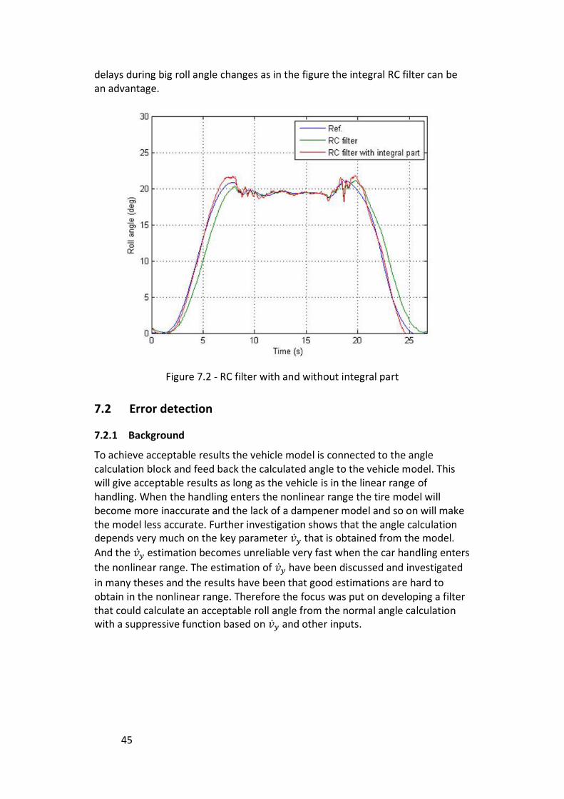
Yaw rate because of slip

As discussed in chapter 3.1.5 problems arise when to big lateral slip is present. The reason to the slip, whether it is because of low friction, a sudden turn or something else, does not matter. A sudden side slip at the front- or the rear-wheels will generate a undesired yaw rate. This yaw rate will in the roll angle equation give a contribution to the centripetal force calculation. But this extra or lesser calculated centripetal force doesn´t exist and is not measured by the accelerometer. Figure 7.3 show a simulation where the car is driving very fast into a banked curve of 10 degrees, all signals for angle calculation is taken from the simulation and is correct. But since the car is slipping the calculations becomes wrong.

Figure 7.3 - Error in eq. 3.13 when slipping

47

7.2.3 Approach

One approach was to investigate what signals had a large derivative or large values when the calculated angle was wrong not trustable. This would allow a detection of when errors in the angle calculation occur. In this part the slip angles were of large interest due to the problems described in 7.2.2 with the car no longer turning around the center of gravity. The other signals that will be investigated are the lateral acceleration, yaw rate, and steering angle.

A reference could be calculated from equation [4.15] with the measured

lateral acceleration and yaw rate, but with the angle set to zero. If the banking angle is constant this would give us a with the same shape like the real but

shifted. Since the banking angle never or seldom changes fast the derivative of the real and the reference described above should be similar. If the derivative

of the estimated differs too much from the derivative of the reference then

the sudden large change in the estimated is unwanted and the angle

calculation cannot be trusted. The last idea was to create an algorithm that would not allow parts of the angle calculation algorithm to grow too fast. This would reduce the spikes that may occur in extreme cases of driving when the parameters in the angle calculation are in the unacceptable area.

Yaw rate because of slip

When the problem of undesired yaw rate occurs this can be filtrated with various filters that filtrate with respect to other signals, as described below. When driving tests on ice were performed the problem with side slippage was quite obvious. Sudden spikes in the estimated roll angle correlated with sudden yaw rate changes. As one task for the Haldex control software is to detect sudden slippage, best results would probably be received if using the existing slippage calculations to filtrate this problem. These signals haven´t been used in this thesis, but is suggested to try as further work.

7.2.1 Results

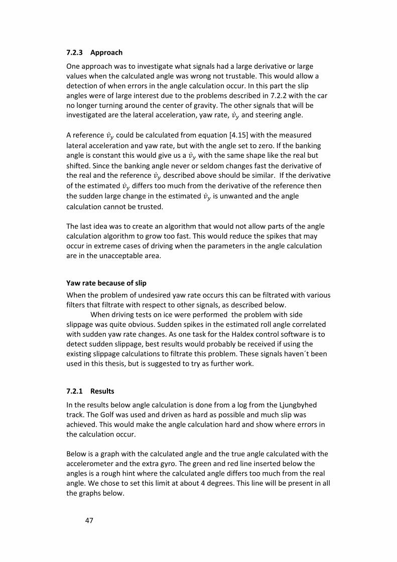
In the results below angle calculation is done from a log from the Ljungbyhed track. The Golf was used and driven as hard as possible and much slip was achieved. This would make the angle calculation hard and show where errors in the calculation occur.

Below is a graph with the calculated angle and the true angle calculated with the accelerometer and the extra gyro. The green and red line inserted below the angles is a rough hint where the calculated angle differs too much from the real angle. We chose to set this limit at about 4 degrees. This line will be present in all the graphs below.

48

All measured values below are shown in their absolute value to easier see the patterns between errors and large values of the investigated parameter.

Figure 7.4 – Calculated and true chassis roll angle

49

Lateral acceleration

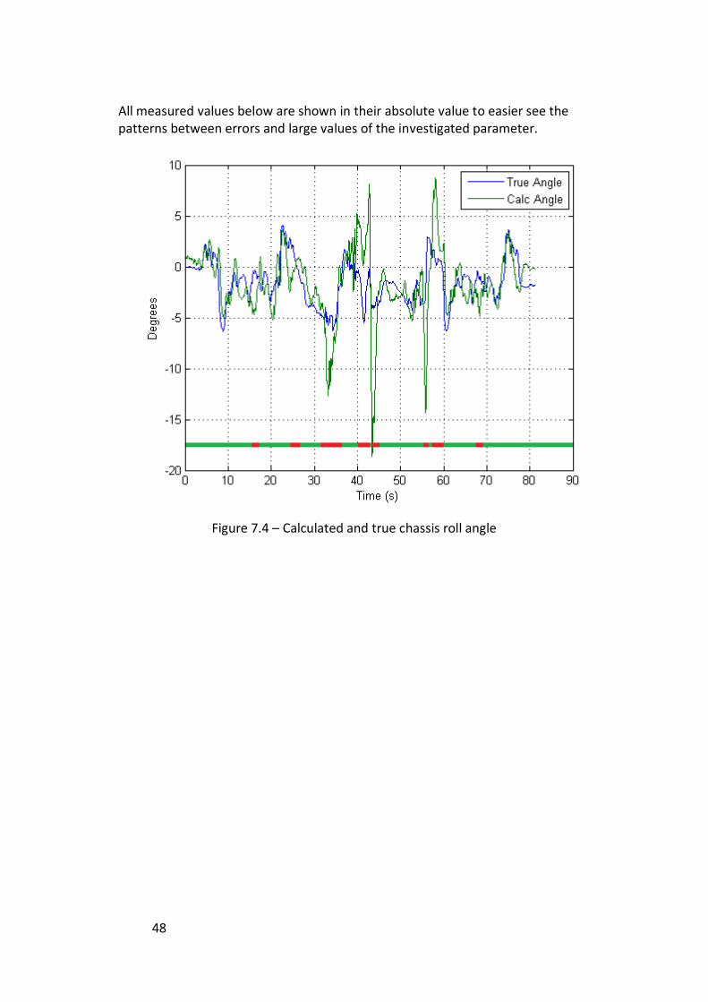
Figure 7.5 – Measured lateral acceleration

When investigating the lateral acceleration we can clearly see that the calculated angle differs from the real angle when the lateral acceleration is in most cases large. The lateral acceleration is also large when the calculated angle is assumed to be correct so the conclusion is that the lateral acceleration is not sufficient to give enough information to detect where the angle calculation algorithm fails.

50

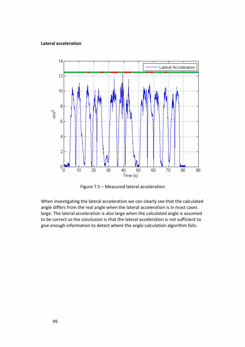
Figure 7.6 – Derivative of measured lateral acceleration

When investigating the derivative of the lateral acceleration the same behavior is found. The derivative can detect when the calculated angle changes fast. This is in some cases due to errors in the angle calculation and in some cases the true value. Therefore the lateral acceleration is of no use when detecting error in the angle calculation.

51

Yaw rate

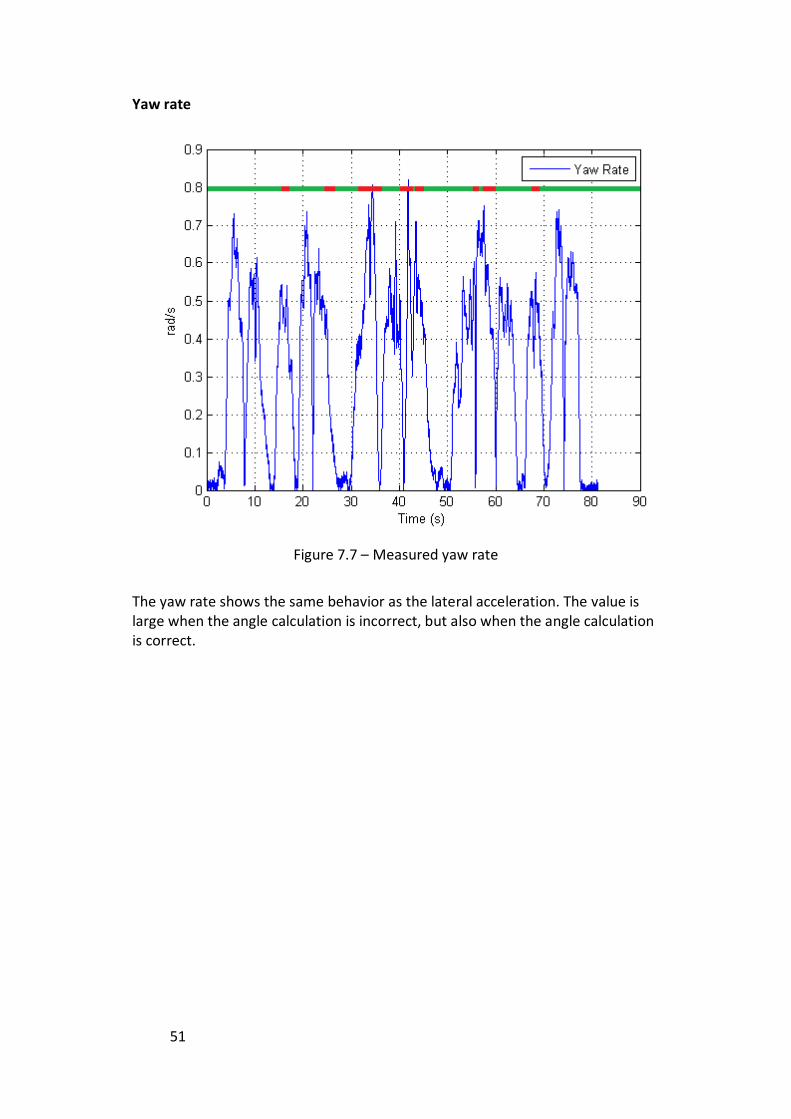
Figure 7.7 – Measured yaw rate

The yaw rate shows the same behavior as the lateral acceleration. The value is large when the angle calculation is incorrect, but also when the angle calculation is correct.

52

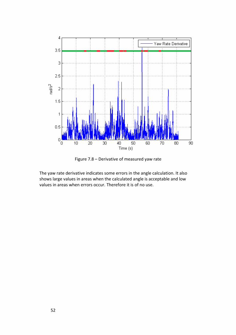
Figure 7.8 – Derivative of measured yaw rate

The yaw rate derivative indicates some errors in the angle calculation. It also shows large values in areas when the calculated angle is acceptable and low values in areas when errors occur. Therefore it is of no use.

53

Steering angle

Figure 7.9 – Steering angle

The steering angle indicates fairly well when the angle calculation algorithm fails and when it works. This is not very surprising since large steering angles cause hard turns which cause skid to occur, especially at high speeds. This means that the vehicles behavior is in the nonlinear range and the estimated values from the model can no longer be trusted, and therefore the angle calculation can no longer be trusted.

54

Figure 7.10 – Derivative of the steering angle

The derivative of the steering angle indicates some errors in the angle calculation. It also shows large values in areas where the calculated angle is acceptable and low values in areas where errors occur. Therefore it is of no use.

55

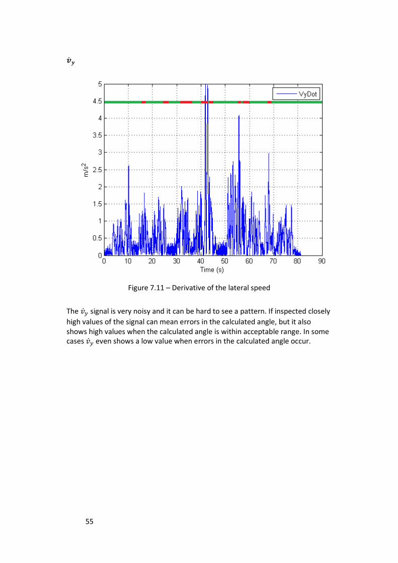
Figure 7.11 – Derivative of the lateral speed

The signal is very noisy and it can be hard to see a pattern. If inspected closely

high values of the signal can mean errors in the calculated angle, but it also shows high values when the calculated angle is within acceptable range. In some cases even shows a low value when errors in the calculated angle occur.

56

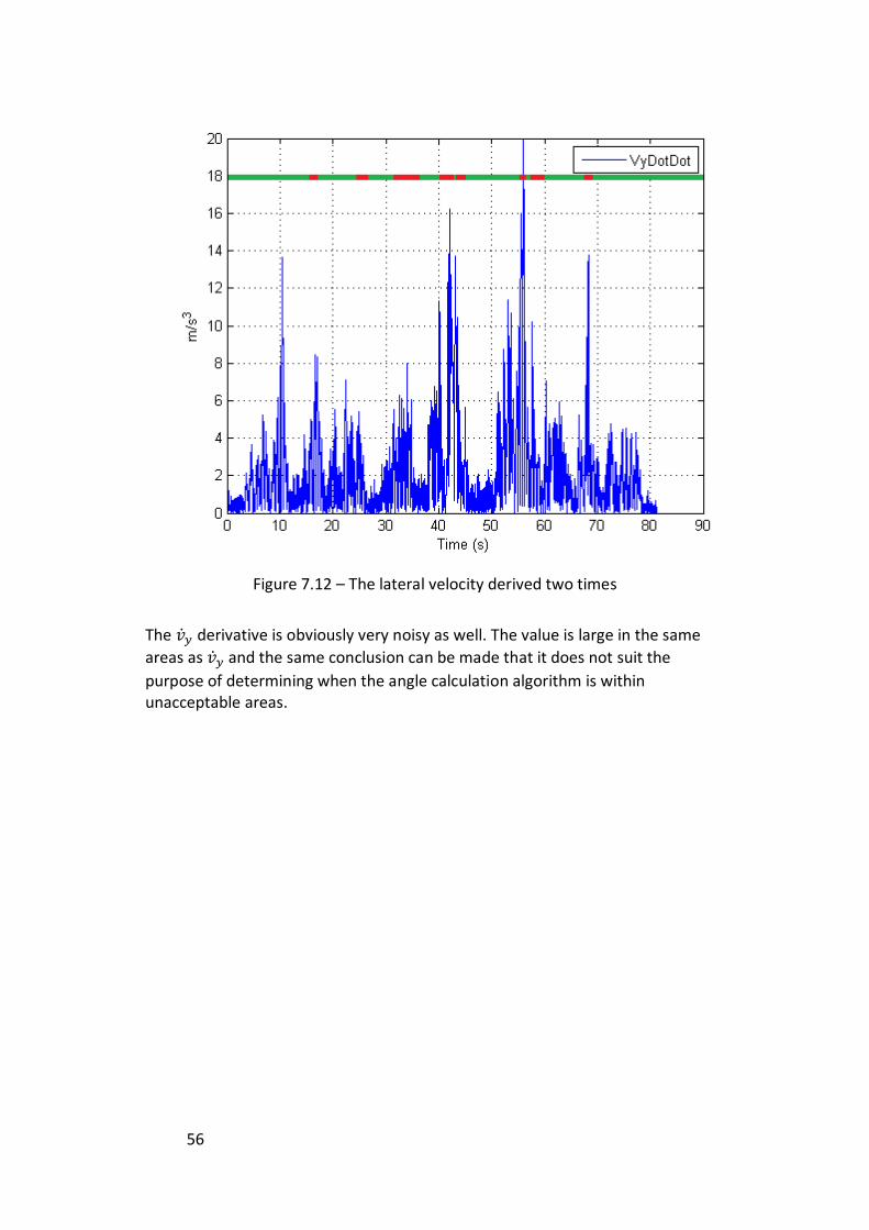
Figure 7.12 – The lateral velocity derived two times

The derivative is obviously very noisy as well. The value is large in the same

areas as and the same conclusion can be made that it does not suit the

purpose of determining when the angle calculation algorithm is within unacceptable areas.

57

Slip angle

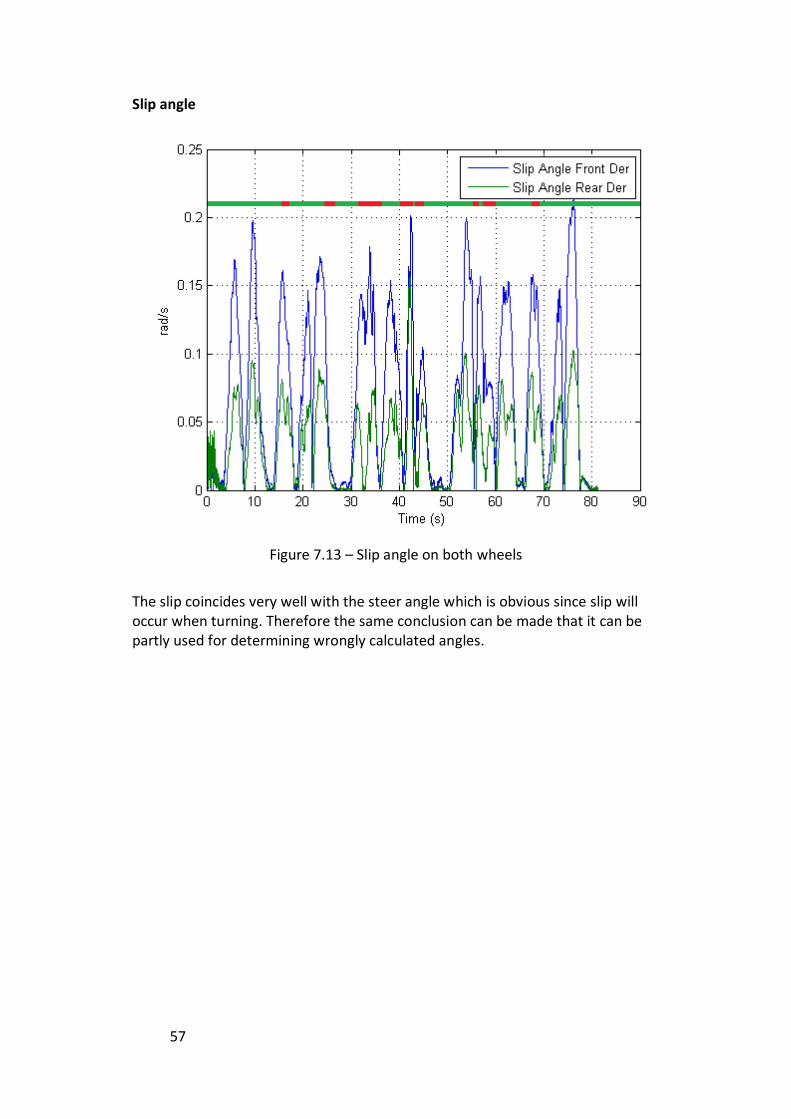
Figure 7.13 – Slip angle on both wheels

The slip coincides very well with the steer angle which is obvious since slip will occur when turning. Therefore the same conclusion can be made that it can be partly used for determining wrongly calculated angles.

58

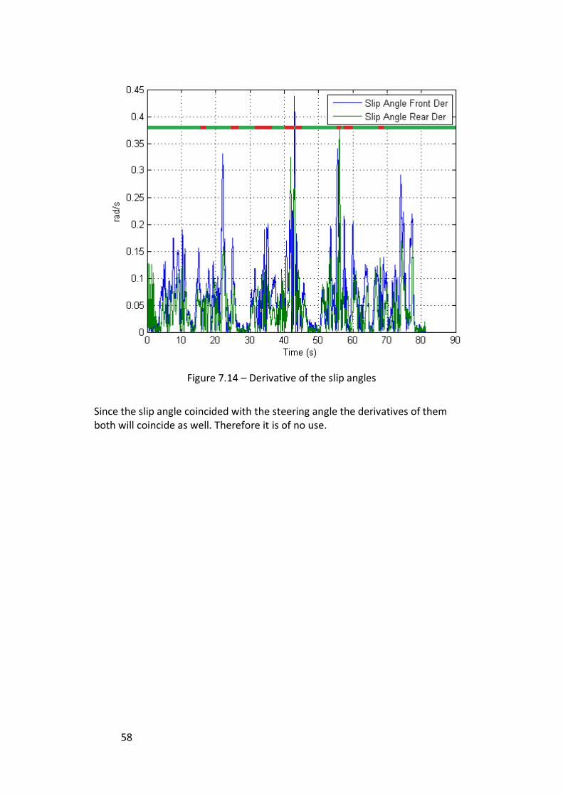
Figure 7.14 – Derivative of the slip angles

Since the slip angle coincided with the steering angle the derivatives of them both will coincide as well. Therefore it is of no use.

59

Difference between VyDot and VyDotRef derivatives

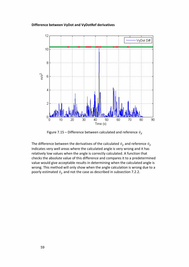
Figure 7.15 – Difference between calculated and reference

The difference between the derivatives of the calculated and reference

indicates very well areas where the calculated angle is very wrong and it has relatively low values when the angle is correctly calculated. A function that checks the absolute value of this difference and compares it to a predetermined value would give acceptable results in determining when the calculated angle is wrong. This method will only show when the angle calculation is wrong due to a poorly estimated and not the case as described in subsection 7.2.2.

60

Angle change derivative

Figure 7.16 – Change in part of the angle calculation algorithm

The graph above shows the derivative of the function:

Large, fast changes in this function will cause the calculated angle to grow fast, which is not credible. It seems like this approach can detect almost every error in the calculation algorithm. The idea behind is to detect fast changes in the angle and therefore it detect the large spikes very well. Unfortunately it also has large values in some areas where the algorithm calculates an acceptable value. But in general this function can be used to detect errors.

7.2.2 Summary

A simple way of error detection is hard to find but some of the methods investigated above proved useful. Since the reason why the errors occur changes many different methods need to be combined to detect most errors. The method of looking at the difference between the estimated and reference

combined with the method of looking at the derivative of a part of the angle calculation algorithm a fairly good approximation can be made of areas where the calculated angle is wrong.

61

When a faulty calculated angle is detected action needs to be taken. The problem is what kind of filtering should be done? This is further investigated in chapter [8.2].

7.3 Different roll angles

As discussed in chapter 3.1 different roll angles exists. The model works best if the chassis roll angle is fed back. This because of the accelerometer placement in the chassis. But it can be desirable to obtain the roll angle of the road. To do this there are different approaches. As seen in Pettersson's thesis one approach is to make a two track model (two parallel bicycle models) and model all four dampers and springs. This will extend the complexity of the model greatly and will be heavy to calculate. Except being complex another drawback of this approach is the fact that springs and dampers can be changed, and their properties may change with time. So the accuracy of a complex model will not necessarily increase.

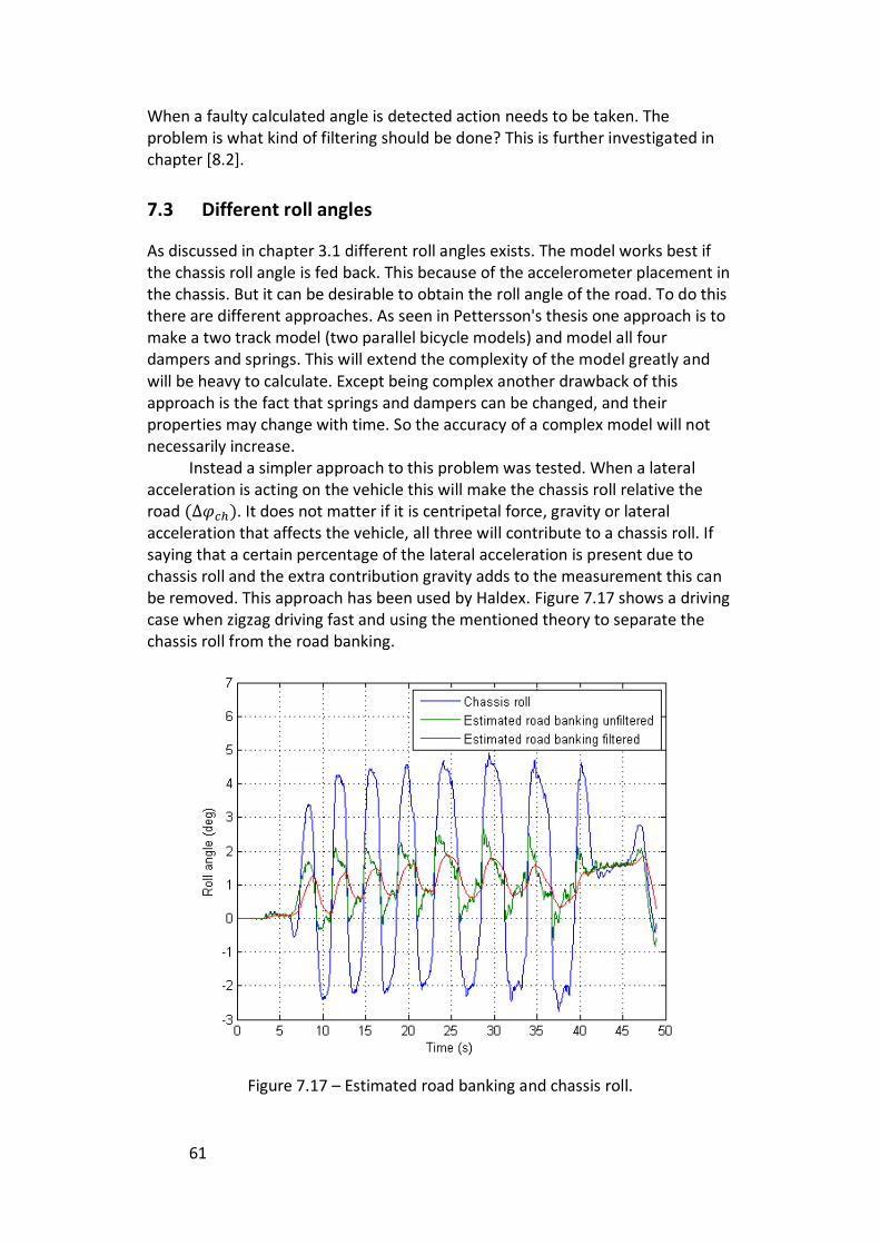
Instead a simpler approach to this problem was tested. When a lateral acceleration is acting on the vehicle this will make the chassis roll relative the road . It does not matter if it is centripetal force, gravity or lateral acceleration that affects the vehicle, all three will contribute to a chassis roll. If saying that a certain percentage of the lateral acceleration is present due to chassis roll and the extra contribution gravity adds to the measurement this can be removed. This approach has been used by Haldex. Figure 7.17 shows a driving case when zigzag driving fast and using the mentioned theory to separate the chassis roll from the road banking.

Figure 7.17 – Estimated road banking and chassis roll.

62

Here it works well, as seen the road is banked about one degree and the car roll about three degrees relative this angle to both sides.

The relationship between lateral acceleration and contributed is set to be linear. But whether this relationship is true or not needs to be investigated more. To get the best results more test need to be made, our guess is that the best result will be achieved by simply measuring the when driving with various lateral accelerations and from experimental data make a lookup table, or low degree polynomial, depending on the results. Unfortunately we have not enough experimental data to achieve this properly.

Another approach to make calculation of road banking better is to filter this angle harder when turbulent driving situations are discovered as discussed in the previous chapter.

Because of the probability of slow changes in road banking a rate limiter that prevents the road banking angle to change faster than a preset value was thought of. This idea works sometimes when very fast disturbances are present, but is in many cases inadequate. However it serves well as a complement to the existing filters.

63

8. Results

8.1 Model and observer

Since the measured lateral acceleration and yaw rate are within acceptable limits focus was put on estimating a that was as close to the true value as possible.

The model that gives good results and is not too complex is the bicycle model upgraded with the roll angle as an additional degree of freedom. The tire model used is the exponential tire model since it gives more accurate results than the linear tire model. The conclusion after testing and evaluating the extended Kalman filter is that the estimated parameters come closer to the true value when the Kalman filter relies much on the measured yaw rate and updates the model using this parameter. The average observer was tested and evaluated as well with good results. The best results were achieved when the model was directly fed with the measured yaw rate, which is the same thing as configuring the average observer to be based on 100% measured yaw rate. The ratio between measured and estimated lateral acceleration was set to between 40-70% measured value and the remaining part from the estimated lateral acceleration from the model. Since the results from both observers were acceptable the average observer is the best choice to use in an application for estimating since it is much lighter

on computations and it is easy to tune. The computational capacity in the vehicles’ micro processors is as stated before limited and therefore all models need to be kept as simple as possible while still providing accurate results.

The calculated angle is a very noisy signal and therefore it needs to be filtered significantly before it is fed back to the model. This filtering is done using a discrete RC filter that uses 98% of the value from the previous sample period and 2% of the calculated angle the current sample period. In some cases of driving large wide peaks occur in the calculated angles which are errors and they will not be removed by this kind of filter. These peaks need to be identified and removed by other means. Ways to indentify wrongly calculated peaks were investigated and discussed in chapter 7.2. To differ between the banking angle and the chassis angle the solution proposed in chapter 7.3 is used. This gives acceptable results but is not an optimal solution as discussed before. The percentage of the lateral acceleration is somewhere between 4-10%, depending on the roll stiffness of the chassis.

64

8.2 Detection of errors and filtering

As stated in the summary in chapter 7.2, there are ways to detect when the calculated angle probably is wrong. The question is what measures to take when a faulty calculated angle is detected. One approach that works fairly well is to output the last calculated value that was not flagged with an error. If the next sample period is not flagged with an error a counter will start counting down. For each step the counter counts down the output will be more based on the newly calculated angle and less on the angle from the previous sample period. This method is easy to tune for either fast response when the calculated angle can be trusted of for slow changes and robustness.

8.3 Simulation results

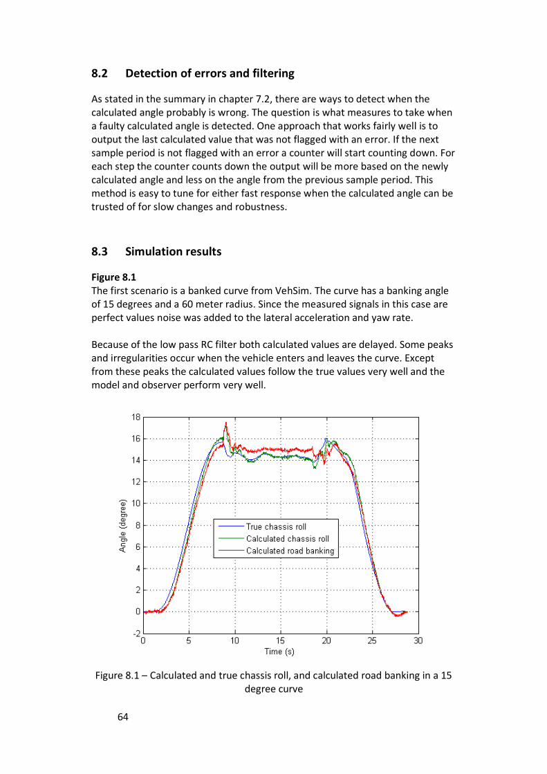
Figure 8.1 The first scenario is a banked curve from VehSim. The curve has a banking angle of 15 degrees and a 60 meter radius. Since the measured signals in this case are perfect values noise was added to the lateral acceleration and yaw rate. Because of the low pass RC filter both calculated values are delayed. Some peaks and irregularities occur when the vehicle enters and leaves the curve. Except from these peaks the calculated values follow the true values very well and the model and observer perform very well.

Figure 8.1 – Calculated and true chassis roll, and calculated road banking in a 15 degree curve

65

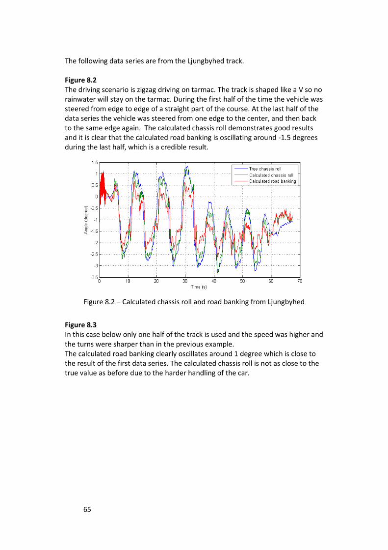
The following data series are from the Ljungbyhed track. Figure 8.2 The driving scenario is zigzag driving on tarmac. The track is shaped like a V so no rainwater will stay on the tarmac. During the first half of the time the vehicle was steered from edge to edge of a straight part of the course. At the last half of the data series the vehicle was steered from one edge to the center, and then back to the same edge again. The calculated chassis roll demonstrates good results and it is clear that the calculated road banking is oscillating around -1.5 degrees during the last half, which is a credible result.

Figure 8.2 – Calculated chassis roll and road banking from Ljungbyhed

Figure 8.3 In this case below only one half of the track is used and the speed was higher and the turns were sharper than in the previous example. The calculated road banking clearly oscillates around 1 degree which is close to the result of the first data series. The calculated chassis roll is not as close to the true value as before due to the harder handling of the car.

66

Figure 8.3 – Calculated chassis roll and road banking from Ljungbyhed

Figure 8.4 In this final example the vehicle was driven around the whole course in racing mode. This pushes the vehicle far into the nonlinear region and will cause the estimated to be incorrect. Therefore the angle calculation cannot be trusted

in some areas. In other areas the calculated chassis roll is within acceptable limits.

Figure 8.4 – Calculated and true values when racing at Ljungbyhed

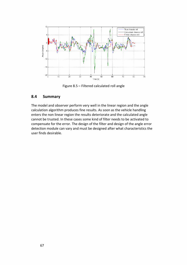
Figure 8.5 A simple filter based on the principle described in chapter 8.2 with a counter is introduced. This produces a more reliable and robust results during the large peaks.

67

Figure 8.5 – Filtered calculated roll angle

8.4 Summary

The model and observer perform very well in the linear region and the angle calculation algorithm produces fine results. As soon as the vehicle handling enters the non linear region the results deteriorate and the calculated angle cannot be trusted. In these cases some kind of filter needs to be activated to compensate for the error. The design of the filter and design of the angle error detection module can vary and must be designed after what characteristics the user finds desirable.

68

9. Discussion and conclusion

Tests of the developed algorithm have proved that a good estimation of the road banking and chassis roll can be achieved. However, it is indeed very difficult to make it work in all imaginable driving cases.

The derived theoretical equation for calculation of the roll angle was improved significantly compared to the one existing at Haldex. Especially by adding the

part. Calculating has shown to be a key to good results.

The problem of yaw rate not affecting the centripetal acceleration is a major drawback for the formula when driving on low friction ground or other cases where large side slips occur. Hopefully this drawback can be improved by using Haldex’s existing control system to detect and prevent sudden incorrect contributions of the yaw rate in the equation.

The bicycle model that was developed for calculation of works well when the

handling of the vehicle is not too extreme. But when larger slip angles occur it performs less well. The feedback of calculated roll angle needs to be filtered very hard, otherwise the system will start to oscillate. But even if it is slow, it works well when calculating . The important thing with the feedback is to feed the

model with larger banking angles. If only driving on a flat surface the model performs well without the feedback.

Both observers developed to update the model with measurements worked well. But tests with the EKF filter showed that it performed better the more the yaw rate was trusted. This leads to the conclusion to use only the measured yaw rate in the model, instead of estimating it, and because of this the EKF was unnecessary. The final choice was the averaging observer, using only measured yaw rate and partially estimated, partially measured lateral acceleration. As presented the model and angle equation often works well, both on flat surfaces and banked curves. Large improvements have been made to the original solution, and a positive outcome of the solution is that a valid on banked

roads is calculated. However the angle calculation is though always some tenth of a second behind the correct one. It is a balance whether a fast response is needed or a more robust one. To improve stability and make sure that shortcomings of the angle equation are minimized, filtering with respect to different signals is needed. It is also here a question of how much disturbances that are allowed or how much the probably correct angle is inhibited.

69

9.1 Future work

Even if improvements have been done in this thesis there are more to be done before implementing this into the real hardware.

We believe that the error detection can be improved by using slip detection already present in today's control software. Usage of already existing algorithms are proposed. To investigate the derived equation 3.13 more and its drawback with yaw rate caused by lateral slip, more tests are proposed. The test should be performed with an extra gyro on the roll axis and a optical velocity sensor to measure the correct longitudinal- and lateral-velocity. The main reason for the optical sensor is to be able to obtain a correct , so it can be evaluated how much the problem

with yaw rate because of slip affects the result. To calculate how much the chassis roll relative the road we have used a linear relationship between measured lateral acceleration present because of chassis roll relative the road. If this is correct should be investigated further. If making more tests on plane ground with different lateral acceleration, a validation or change, of the existing relationship could be done. At last, our solution should be tested more to better evaluate how it performs in many different driving cases.

70

10. Nomenclature

10.1 Expression explanation

x-axis axis in vehicle travel direction y-axis axis to the left when facing forward z-axis axis upwards roll angle around x-axis according to the right hand rule yaw angle around z-axis according to the right hand rule roll rate angular velocity around x-axis yaw rate angular velocity around z-axis

10.2 Physical units

Symbol Units Description roll angle vehicle chassis road banking angle vehicle chassis roll angle relative road

yaw rate vehicle gravitation Vehicle longitudinal velocity Vehicle lateral velocity

Vehicle lateral velocity derivative

Measured lateral acceleration

Lateral acceleration due to normal forces from

gravitation Lateral acceleration due to centripetal force

Turning radius Steering wheel angle Lateral tire force front tires

Lateral tire force rear tires

Tire normal force Vehicle mass Yaw torque Moment of inertia Slip angle front

Slip angle rear

71

11. References

[1] Pacejka, Hans B. 2006. Tire and Vehicle Dynamics - Second Edition. Oxford : SAE International, 2006. ISBN 0 7680 1702 5.

[2] Welch, Greg. Bishop, Gary. An Introduction to the Kalman Filter. (1)

University of North Carolina at Chapel Hill, 2006.

[3] Ding, Zhimin. AN715 – Kalman filter implemented in the XA eases sensory fusion. Philips Semiconductors, 1999.

[4] Rill, Georg. 2006. First Order Tire Dynamics. University of Applied

Sciences Regensburg.

[5] Wennerström, E. Nordmark, S. Thorvald, B. 1999. Fordonsdynamik. Kungliga Tekniska Högskolan.

[6] Wittenmark, B. Åström, K. Årzén, K. 2009 Computer Control: An

Overview Educational Version 2009. Lund University, 2009.

[7] http://www.ece.ucsb.edu/~roy/classnotes/147b/lecture4_small.pdf, 2010-11.

[8] http://www.trafikverket.se/TrvSeFiler/Foretag/Bygga_och_underhalla/Vag/Vagutformning/Dokument_vag_och_gatuutformning/Vagar_och_gators_utformning/Linjeforing/08_tvarfall.pdf, 2010-11.

[9] Pettersson, Pierre. 2008. Estimation of Vehicle Lateral Velocity. Haldex Traction & Lund University, 2008.

[10] Schoutissen, S.L.G.F. 2004. Design and Validation of a Vehicle

State Estimator. Haldex Traction & TU Delft, 2004.

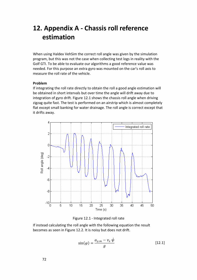
72

12. Appendix A - Chassis roll reference estimation

When using Haldex VehSim the correct roll angle was given by the simulation program, but this was not the case when collecting test logs in reality with the Golf GTI. To be able to evaluate our algorithms a good reference value was needed. For this purpose an extra gyro was mounted on the car's roll axis to measure the roll rate of the vehicle. Problem If integrating the roll rate directly to obtain the roll a good angle estimation will be obtained in short intervals but over time the angle will drift away due to integration of gyro drift. Figure 12.1 shows the chassis roll angle when driving zigzag quite fast. The test is performed on an airstrip which is almost completely flat except small banking for water drainage. The roll angle is correct except that it drifts away.

Figure 12.1 - Integrated roll rate

If instead calculating the roll angle with the following equation the result becomes as seen in Figure 12.2. It is noisy but does not drift.

[12.1]

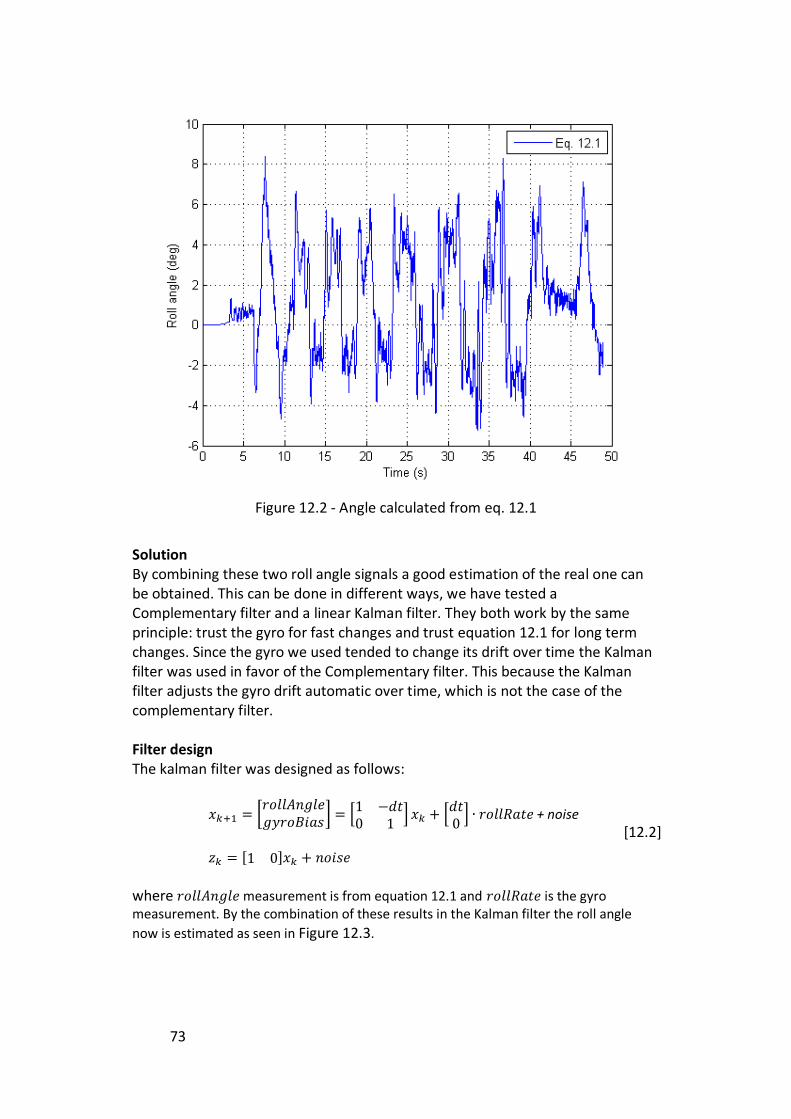
73

Figure 12.2 - Angle calculated from eq. 12.1

Solution By combining these two roll angle signals a good estimation of the real one can be obtained. This can be done in different ways, we have tested a Complementary filter and a linear Kalman filter. They both work by the same principle: trust the gyro for fast changes and trust equation 12.1 for long term changes. Since the gyro we used tended to change its drift over time the Kalman filter was used in favor of the Complementary filter. This because the Kalman filter adjusts the gyro drift automatic over time, which is not the case of the complementary filter. Filter design The kalman filter was designed as follows:

+ noise

[12.2]

where measurement is from equation 12.1 and is the gyro measurement. By the combination of these results in the Kalman filter the roll angle

now is estimated as seen in Figure 12.3.

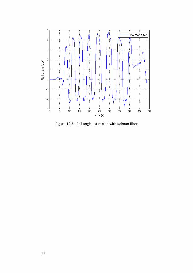
74

Figure 12.3 - Roll angle estimated with Kalman filter

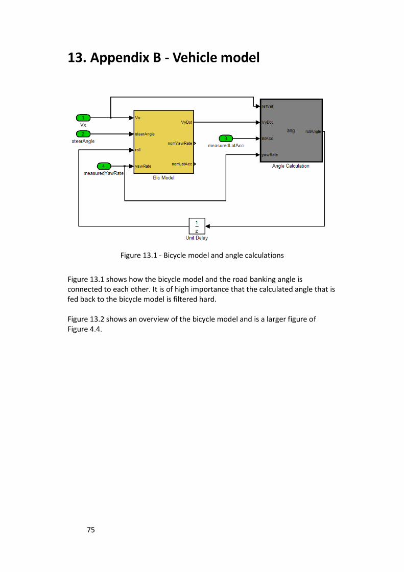
75

13. Appendix B - Vehicle model

Figure 13.1 - Bicycle model and angle calculations

Figure 13.1 shows how the bicycle model and the road banking angle is connected to each other. It is of high importance that the calculated angle that is fed back to the bicycle model is filtered hard. Figure 13.2 shows an overview of the bicycle model and is a larger figure of Figure 4.4.

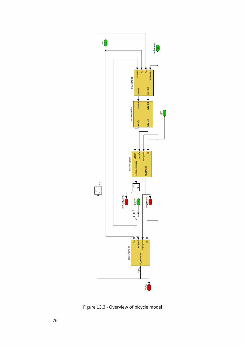
76

Figure 13.2 - Overview of bicycle model