estimation of inﬁnite dilution activity coefﬁcients of...

Estimation of Infinite Dilution Activity Coefficients ofOrganic Compounds in Water with Neural Classifiers

Francesc Giralt and G. EspinosaDepartament d’Enginyeria Quımica, ETSEQ, Universitat Rovira i Virgili, Tarragona, Catalunya, Spain

A. Arenas and J. Ferre-GineDepartament d’Enginyeria Informatica i Matematiques, ETSE, Universitat Rovira i Virgili, Tarragona, Catalunya, Spain

L. Amat, X. Girones, and R. Carbo-DorcaInstitut de Quımica Computacional, Universitat de Girona, Girona, Catalunya, Spain

Y. CohenDept. of Chemical Engineering, University of California, Los Angeles, CA 90095

DOI 10.1002/aic.10116Published online in Wiley InterScience (www.interscience.wiley.com).

A new approach is presented for the development of quantitative structure–propertyrelations (QSPR) based on the extraction of relevant molecular features with self-organizingmaps and the use of a modified fuzzy-ARTMAP classifier for variable prediction. The presentmethodology is demonstrated for the development of a QSPR for the aqueous-phase infinitedilution activity coefficient ��, based on a data set of 325 diverse organic compounds. TheQSPR was developed using a set of 11 molecular descriptors (four connectivities v�1–4,Coulomb self-similarity measure, electron–nuclear attraction, dipole moment, sum of atomicnumbers, number of filled levels, average polarizability, and nuclear–nuclear repulsion). Thefinal set of molecular descriptors was selected from an initial pool of 23 topological andquantum chemical descriptors, including six molecular quantum similarity measures, bymeans of a topological analysis of self-organization of the data set. Additional interpolatedinformation to enhance the training of the neural system was obtained from the self-organi-zation analysis. The resulting fuzzy-ARTMAP–based QSPRs performed with errors that wereon the average seven times smaller compared to previous published models. The use of onlyfour molecular quantum similarity measures proved to be sufficient for building a ln��

fuzzy-ARTMAP–based QSPR with reasonable accuracy. © 2004 American Institute of ChemicalEngineers AIChE J, 50: 1315–1343, 2004Keywords: self-organizing maps, fuzzy-ARTMAP neural classifier, QSPR, infinite dilutionactivity

Introduction

The distribution of organic chemicals in the environment isaffected by their physicochemical and thermodynamic proper-

ties, among which air–water partitioning (or Henry’s law con-stant) and aqueous solubility are of particular importance(Mackay et al., 1992; Yalkowsky, 1999; Yalkowsky and He,2003). Knowledge of the above parameters is of fundamentalinterest and also of importance in various industrial processes(Fredenslund et al., 1975; Mackay et al., 1992) and in ground-water remediation by air stripping. The Henry’s law constant ofsparingly water soluble organics is directly proportional to the

Correspondence concerning this article should be addressed to F. Giralt [email protected].

© 2004 American Institute of Chemical Engineers

AIChE Journal 1315June 2004 Vol. 50, No. 6

infinite dilution activity coefficient ��, which in turn is essen-tially inversely proportional to the aqueous solubility. Theinfinite dilution activity coefficient is a fundamental thermo-dynamic parameter important for the estimation of aqueoussolubility and Henry’s law constant (Fredenslund et al., 1975;Mackay et al., 1992).

Various theoretical models and group contribution methodsfor predicting activity coefficients in dilute solutions have beenproposed in the literature (Fredenslund et al., 1975; Lazaridisand Paulaitis, 1993; Mackay and Shiu, 1977; Mackay et al.,1992; Medir and Giralt, 1982; Mitchell and Jurs 1998; Sher-man et al., 1996; Tochigi et al., 1990). These predictions havebeen successful when dealing with athermal systems and, to alesser extent, with polar systems. For example, it has beenshown that the combinatorial term in UNIFAC is underesti-mated, whereas the residual is overestimated (Voutsas andTassios, 1996) when dealing with aqueous mixtures and withincreasing polarity of the organic solute. The modification ofthe combinatorial and residual terms in the original UNIFACmodel has significantly improved predictions for athermal sys-tems but such modifications have been less satisfactory forpolar systems (Voutsas and Tassios, 1997). Alternative ap-proaches that are specifically designed for aqueous solutions,such as the linear solvation energy relationship (LSER; Sher-man et al., 1996), might be more accurate (average absolutedeviation of 0.294 ln�� units for 336 organics in aqueoussystems).

Improvements of group contribution methods by direct cal-culations of interaction energies are possible by means ofquantum chemical or variational methods; however, suchmethods are typically computationally demanding and re-stricted to relatively small molecules (Sandler, 2002). A briefreview on the application of computational quantum chemistrymethods, either to obtain the interaction energy surface for apair of molecules or to improve current group contributionmethods by less intensive calculations, can be found elsewhere(Sandler, 2002).

Over the last three decades various quantitative structure–property relationships (QSPRs) have been proposed to estimate�� for organics in water. The premise of QSPRs is that there isa unique relationship between molecular chemical descriptorsand a target physicochemical property. Given a selected set ofmolecular descriptors, one searches for optimized correlationsbetween the descriptors and the desired chemical specific prop-erty. For example, Mackay and Shiu (1977) correlated theaqueous phase ln�� for hydrocarbons with the number ofcarbon atoms. Medir and Giralt (1982) correlated ln �� foraliphatic and aromatic hydrocarbons using molecular descrip-tors that included the first-order molecular connectivity index,surface area, dipole moment, number of carbon atoms, totalelectronic energy, and acentric factor. Mitchell and Jurs (1998)applied several correlation techniques and perceptron neuralnetworks to estimate ln��. They used three topological descrip-tors, four charged partial surface area (CPSA) indices, twohydrogen bonding descriptors, heat of formation, and twotheoretical linear solvation energy relationship (TLSER) indi-ces to describe the basicity of hydrogen bonding. Also noted isa related study by Yalkowsky and Valvani (1979), in which theaqueous solubility of organic compounds was correlated withthe molecular surface area, and a series of studies byYalkowsky and coworkers (Peterson and Yalkowsky, 2001;

Ran and Yalkowsky, 2001; Ran et al., 2001; Yang et al., 2002)that contributed significantly to this area of aqueous solubilityestimation with models based on group contribution or frag-ment structural information.

Backpropagation neural networks have recently emerged asan alternative for the development of QSPRs and quantitativestructure–activity relationships (QSARs) to predict physico-chemical properties and biological activities, respectively(Bunz et al., 1998; Chow et al., 1995; Egolf and Jurs, 1993;Espinosa et al., 2000, 2001a,b; Gakh et al., 1994; Hall andStory, 1996; Mitchell and Jurs, 1998; Simamoea et al., 1993;Stanton and Jurs, 1990; Stanton et al., 1991; Viswanadhan etal., 2001; Yaffe et al., 2001, 2003). This alternative modelingstrategy for QSPR development yields significantly higherprediction accuracy compared to that of traditional regression-based correlations. For example, the 12–6–1 neural networkmodel proposed by Mitchell and Jurs (1998), to estimate ln��

of organics in water, performed with an average root-mean-square error of 0.376 ln units, 0.406 ln units, and 0.434 for thetraining (271 compounds), validation (25 compounds), and test(25 compounds) sets, respectively. Also, 92 �� values of 19halocarbons in water and 18 organic compounds in five hy-drofluoroparaffins solvents over a temperature range of 291–333 K were predicted by Rani and Dutt (2002) with a feedfor-ward network trained with 351 data points, with an averageabsolute deviation of 11.8% on the basis of ��, compared with94.3% obtained by multilinear regression. The interpretation ofresults obtained with these feedforward neural architectures isnot straightforward, given that the structure–property or struc-ture–activity relationships are embedded within the weightsdistributed within the network. More recently, neural network–based QSPRs and QSARs (Espinosa et al., 2002, 2003;Gasteiger et al., 1994a,b) have been developed based on Ko-honen (self-organizing or feature maps) and ARTMAP neuralnetwork architectures. This latter approach proved to be par-ticularly useful in the recognition of coherent structures em-bedded in turbulent flows (Ferre-Gine et al., 1996) and in thedevelopment of industrial virtual sensors (Rallo et al., 2002a,b)attributed to the ability of these algorithms to classify patternsin complex data sets, even in the presence of other correlatedinformation and noise.

The current study presents a comprehensive approach todeveloping neural network–based QSPR for the aqueous infi-nite dilution activity coefficient of organics based on a predic-tive fuzzy-ARTMAP architecture and the use of self-organiz-ing maps (SOMs), also known as a Kohonen neural network(Kohonen, 1982, 1990), for extracting molecular features rel-evant to the target property. The initial set of descriptors wasselected to contain topological and quantum molecular infor-mation to capture both two- and three-dimensional (3-D) (Carbo-Dorca and Besalu, 1998; Cramer et al., 1988) information(such as conformational, stereochemical, electronic, and bind-ing information). The present set of descriptors also includedmolecular quantum similarity measures (MQSM; Carbo-Dorcaand Besalu, 1998). The selection of the most suitable set ofdescriptors from the initial set was accomplished with a SOManalysis, which also served to identify chemical classes andtheir characteristics with respect to the molecular informationincluded in the set of descriptors. In addition, in the currentwork we demonstrate that the integration of SOM with fuzzyARTMAP (Carpenter et al., 1987, 1991, 1992; Giralt et al.,

1316 AIChE JournalJune 2004 Vol. 50, No. 6

2000) improves not only the accuracy and predictive capabil-ities of the QSPR (Espinosa et al., 2002, 2003) but enables oneto explore the relative contribution of any given descriptor (orgroup of descriptors), with respect to both chemical classifica-tion and estimation of the target property.

Neural Network ArchitecturesKohonen self-organizing maps: cluster analysis andselection of descriptors

The Kohonen neural network is a self-organizing map suit-able for classification analysis (Erwing et al., 1992; Kaski andLagus, 1996; Kohonen, 1982, 1990; Vesanto, 1999). In thepresent work SOM analysis was used to: (1) select the mostsuitable set of descriptors by measuring the dissimilarity of thedifferent maps that are formed when clustering into the nodesof the map the complete set of compounds according to theirmolecular characteristics, as specified by different sets of mo-lecular descriptors and the target ln�� variable; and (2) use thevectors characterizing each neuron or node in the trained map,that is, the prototype vectors of clustered compounds into thenodes during training, in addition to the compounds them-selves, to train the fuzzy-ARTMAP–based QSPR.

A self-organizing map automatically adapts itself such thatsimilar inputs are associated with topologically close units (orneurons) in a two-dimensional (2D) grid. During the trainingprocess, N-dimensional input data are self-organized in a dis-cretized 2D plane formed usually by a grid of K � K units. Thenumber of units is specified based on the sought populationdistribution of input data among the neurons, in such a way thatclose input vectors of descriptors characterizing compounds inthis N-dimensional space are mapped into close-neighborhoodneurons while minimizing the number of empty or over-crowded classes. The SOM type of neural network is especiallyuseful for capturing underlying relationships within the inputdata. Briefly, the main steps in the generation of a SOM are asfollows:

(1) An input vector xi of dimension N is presented to thenetwork. Each cycle of presentation including all input vectorsxi is called an epoch.

(2) The Euclidian distance between this input vector and allnodes (neurons) in the network lattice is calculated, as follows

�j � �i�0

N�1

� xi�t� � wij�t��2 (1)

where xi(t) is the ith component of the N-dimensional inputvector and wij(t) is the connection strength (weight) betweenthe input vector component i and the mapping array node j atposition t, in the sequence of data presentation to the network.Initially these weights are assigned random values.

(3) Node j* with the minimum distance �j defined by Eq. 1is selected as the winner neuron or best matching unit (BMU).

(4) The weights of node j* and those of its neighbor nodes,identified by the neighborhood Nj*(t), are updated

wij�t � 1� � wij�t� � ��t�� xi�t� � wij�t�� (2)

for j � Nj*(t) and 1 � i � N.

The function �(t), which decreases monotonically over theenvironment of the winner neuron, defines the region of influ-ence that the input vector has on the SOM. This function isdefined by the neighborhood function �0 and the learning rate(t) according to

��t� � �0��rc � r�, t��t� (3)

where r is the location of the units or neurons on the grid of themap. The simplest neighborhood function is the bubble func-tion, which is constant over the whole neighborhood of thewinner neuron (node) and zero elsewhere (Kaski and Kohonen,1994; Vesanto, 1999). However, a more convenient function isthe Gaussian neighborhood function, defined by

�0 � exp��rc � r�2

22�t� � (4)

where the neighborhood radius (t) self-adapts after each ep-och. The type of neighborhood function and the number ofneurons determine the sensitivity and the granularity of themap, respectively. Finally, it is noted that the learning rate (t)in Eq. 3 is a decreasing function of t over the range [0, 1] andit is usually defined by the power series

�t� � 0�T

0� t/T

(5)

where 0 and T are the initial and final learning rates, respec-tively, and T is the size of the training set cycles (i.e., thenumber of epochs selected for training).

The trained SOM can be used to visualize different featuresof the data (Kaski and Kohonen, 1994; Vesanto, 1999). Thegraph representations of the clustered set of data into the nodesof the map facilitate a clearer identification of the underlyingrelationships among data. This is accomplished by visualizingeither the matrix of distances between nodes (U-matrix) or thecontribution of different input information into this organiza-tion [component planes (C-planes)]. A component plane is thedistribution over the map of the values of one of the elements(weights wij) of the vectors (prototypes) characterizing eachneuron or node. Visualization and analysis of the SOM wereaccomplished using the Matlab SOM toolbox, as reportedelsewhere (Kaski and Kohonen, 1994; Vesanto, 1999).

Identification of prototype classes of compounds and selec-tion of relevant descriptors required setting the optimal size ofthe SOM. The optimal SOM size should accommodate, duringtraining, the compounds characterized by the N moleculardescriptors of the pool (that is, initial set) plus the targetvariable ln�� into the K � K grid units, with about 80% of thenodes occupied by compounds to ensure both continuity ofclusters within the nodes of the map and a sufficient populationdensity per node. The above ensures the generation of compactclusters in the nodes [that is, small average distance (n) be-tween the members of each cluster], and that all nodes, whetheror not occupied by clustered compounds, are trained accordingto Eqs. 2 and 3. Subsequently, a curvilinear component anal-ysis and/or visual inspection of the component C-planes cor-responding to all descriptors was carried out to identify simi-


larities in clustering topology (that is, how each descriptorclustered the compounds in the nodes in relation to the targetvariable ln��). Thus, descriptors favoring a similar topology ordistribution of compounds among the nodes (clusters) in themap could be identified as similar and grouped into a commonclass of descriptors with respect to the target variable. Descrip-tors were ordered by picking from each class of similar de-scriptors those with the highest correlation or absolute covari-ance, with the restriction that each absolute covariance with thetarget variable was higher than the average value for the poolof descriptors (that is, the complete set of descriptors). Theordering process continued by sorting indices according to thevalue of the absolute covariance. Following this procedure(Espinosa et al., 2002), nonredundant information of the dif-ferent classes of descriptors, formed by grouping their respec-tive C-planes, as well as their correlation with respect to thetarget variable, were accounted for in the construction of themost suitable set of descriptors.

The most representative set (that is, most suitable set) ofdescriptors was defined as the set with the smallest number ofdescriptors that provided the highest representation of the com-pound data set as determined by the SOM analysis. The selec-tion was carried out by first selecting the most descriptive indexfrom each of the N self-organizing maps, and then successivelyadding the remaining indices in the order of decreasing covari-ance with the target variable. To determine when all relevantinformation had been considered in the succession of N SOMs,changes in topology caused by the progressive incorporation ofthe molecular information were quantified. This was accom-plished by measuring the dissimilarity between any of twomaps L and M. Dissimilarity was defined as the averageddifference in the SOM representation of the sample vectorsused for training, as follows

D�L, M� � E�dL� x� � dM� x�

dL� x� � dM� x�� (6)

in which E is the average expectation, the subscripts L and Mdesignate the two different maps, and d(x) is the distance fromx to the second BMU, denoted by mc(x), beginning at the firstBMU or winner neuron, denoted by mc(x). Of all possible pathsbetween mc(x) and mc(x) the shortest continuous path

d� x� � � x � mc� x�� mini

�k�0

Kc� x��1

�mIi�k� � mIj�k1�� (7)

between neighbor units was selected. This distance, which issimilar to that first proposed by Kaski and Lagus (1996),reflects the continuity of the SOM. Also, it indicates the rela-tive capacity of any map to represent the data set when trainedwith compounds characterized by a given number of descrip-tors with respect to any other map trained using more or fewerdescriptors.

The smallest average dissimilarity value calculated by ap-plying Eq. 6 to the SOMs, corresponding to all combinations ofthe ordered pool of descriptors, indicates the maximum coher-ence and compactness of the information represented by thatparticular map. Thus, the process of including indices to formthe most suitable set of molecular descriptors can conclude

when the average dissimilarity measure of the correspondingmap with the rest of maps stabilizes. The above dissimilarityanalysis provides a systematic methodology of determiningsimilarity among maps even when the dimension or number ofindices of the input vectors may be very different. The indicesof SOM with minimal average dissimilarity provide a goodrepresentation of all clusters of compounds formed in the nodesand constitute the most suitable set of molecular descriptors forQSPR modeling (Espinosa et al., 2002).

Fuzzy ART and Fuzzy ARTMAP

The selection of a neural architecture with predictive capa-bilities has been the subject of numerous studies in relation totime series analyses (Cybenko, 1989; Fessant et al. 1995; Giraltet al., 2000; Hornik et al. 1989), data mining (Agrawal et al.,1993; Bishop, 1995; Fayyad, 1996; Hertz et al., 1991), orpattern recognition (Agrawal et al., 1993; Ferre-Gine et al.,1996; Gutfreund and Mezard, 1988; Hecht-Nielsen, 1995;Hertz et al., 1991). The most commonly used architecture inthe above fields and in other engineering applications has beenthe multilayer perceptron (Bishop, 1995; Hertz et al., 1991)with the learning mechanism of backpropagation. This ap-proach is simple to use, has a sound mathematical foundation,and yields excellent results for most engineering applications.However, it is not suitable when pattern recognition or featureextraction capabilities are desired because relationships be-tween variables in such networks are embedded within theweights in a distributed form (Bishop, 1995; Hecht-Nielsen,1995; Hertz et al., 1991). In difficult problems involving pat-tern recognition, such as those found in the development ofQSPRs for data sets of heterogeneous compound classes, it isadvantageous to use neural network classifiers, as shown in anumber of recent studies (Espinosa et al., 2000, 2001b, 2002,2003; Yaffe et al., 2001, 2003) on QSPR development.

One of the most powerful classifiers is ARTMAP, which isbased on adaptive resonance theory (ART) and has been shownto be capable of learning the dynamics of large-scale structuresin a turbulent wake flow (Giralt et al., 2000). The application offuzzy ARTMAP networks for QSPR development (Espinosa etal., 2002) has several advantages because of their capability toclassify and analyze noisy and incomplete data sets with areduced number of required model parameters and avoidanceof local minima trapping (Carpenter et al., 1987, 1991, 1992).This architecture is also sufficiently transparent to allow con-tinuous checking of the goodness of the classification duringthe training process, as well as how the relationships betweenthe inputs and the outputs are established.

Adaptive resonance theory (ART) initially emerged fromresearch on human cognitive information processing (Carpen-ter et al., 1987, 1991). Fuzzy ARTMAP (Carpenter et al., 1992) isone of the algorithms of the ART family that overcomes thestability–plasticity dilemma by creating as many new classes asneeded to incorporate new information presented to the network ina stable manner while preserving the old knowledge contained inpreviously created classes. It associates prototypes of input pat-terns with their target outputs. The key feature is a control param-eter that measures the similarity between the prototype patterns,stored in different network categories or classes, and any currentinput pattern. If the control parameter (vigilance) is not satisfiedwithin a given accuracy, a new class or category is created during


learning. As a result, the number of categories (or prototypevectors) grows until a network structure has been built that is ableto model the output based on the input data.

The architecture of fuzzy ARTMAP consists of two fuzzyART modules, ARTa and ARTb, interconnected by a map field,Fab, as shown in Figure 1. The ARTa (ARTb) module has twolayers of nodes: F1a (F1b) is the input layer and F2a (F2b) is adynamic layer where each node (class or category) encodes aprototype of a cluster of the input patterns. The number of suchnodes can be increased when necessary. During supervisedlearning, an input pattern vector (molecular descriptors) is fedto the ARTa module and the output vector (target variable) toARTb. These are independently classified in each module. Amap field (Fab) adaptively associates prototype nodes in ARTa

with their respective target classes in ARTb. The node with thehighest value of the activation function is selected as thewinner, and all other nodes are suppressed in accordance withthe winner-take-all rule (Carpenter et al., 1987, 1991, 1992).

The search cycle ends when either the current prototype isable to satisfy the vigilance parameter criterion (accuracy in theclassification) or a new node is recruited in F2a with the inputpattern coded as its prototype pattern. During testing only thecategory F2b layer is activated so that for any input presentedto F1a an output can be effected from F2b, according to thepredictive fuzzy ARTMAP system proposed by Giralt et al.(2000). The network reaches a resonant state when a categoryprototype vector matches the current input vector sufficiently

such that the orienting subsystem will not send a reset signal tothe F2 layer. The network learns only in its resonant state,where it is capable of developing stable classification of arbi-trary sequences of input patterns by self-organization. Thevoting strategy of training the system several times, usingdifferent orderings of the input set, not only improves predic-tions but can also be used to assign confidence estimates tocompeting predictions when dealing with small, noisy, or in-complete training sets. Further information on this issue and onthe ART family of neural networks can be found elsewhere(Carpenter et al., 1987, 1991, 1992).

Data Set and Molecular Descriptors

The present aqueous infinite dilution activity coefficient ��

data set consisted of 325 organic compounds, originally com-piled by Sherman et al. (1996) and later also used by Mitchelland Jurs (1998), to correlate the aqueous phase ln�� withmolecular descriptors. This heterogeneous data set includeshydrocarbons, alcohols, ethers, aldehydes, ketones, acids, ha-logenated hydrocarbons, amines, amides, nitriles, and com-pounds containing sulfur. The complete data set, with thecorresponding ln�� values, is included in the supporting infor-mation (see Table 5 below). A subset of 280 compounds wasselected for training (tr) and 45 compounds were used fortesting (te) the fuzzy-ARTMAP–based QSPR models. Bothdata sets were selected by a fuzzy ART (Carpenter et al., 1987,

Figure 1. Fuzzy ARTMAP architecture.


1991, 1992) neural system following the procedure describedby Espinosa et al. (2001b), to ensure that the training setrepresented the complete data set. The 10 � 10 SOM trained toidentify the most suitable molecular information, in relation tothe target ln �� property, contained the classified informationof the input data among the prototype vectors representing thenodes with clustered compounds (that is, the occupied nodes ofthe map). The map also contained interpolated information inthe prototype vectors of empty nodes because they were alsotrained as neighbors of occupied (winning) nodes by Eqs. 2 and3. Thus, the current work also explores the benefit of using theinformation of the 100 prototypes of the map for training thecurrent fuzzy-ARTMAP–based QSAR model, in addition tothe 280 compounds of the training set. In this latter case,however, the 10 � 10 SOM was built from training informa-tion only (280 compounds) to avoid contaminating these pro-totypes with test information.

An initial set of 23 molecular descriptors was first developedfollowing the criteria and procedure described below. An op-timal (that is, most suitable) subset consisting of the minimumnumber of descriptors that also provided the relevant informa-tion necessary to develop the present QSPR was then obtained.In this systematic selection process (Espinosa et al., 2002) allindices were classified according to the topology of their C-planes in the SOM (i.e., according to their similar capability tocluster compounds in the 10 � 10 nodes of the map). Thus,both the most representative indices from these C-plane classesand those with the highest correlation with the target variablecan be selected.

The initial pool (that is, initial set of descriptors) was formedwith the topological and quantum chemical descriptors consid-ered in the studies of Medir and Giralt (1982) and Yaffe et al.(2001) to respectively predict ln�� of hydrocarbons in waterand aqueous solubilities of diverse set of organic compounds.Topological indices provide information about the adjacency ofthe atoms in the molecular structure. Among those more fre-quently used in QSPRs are the Wiener index (Wiener, 1947),the connectivity indices used by Randic (Randic, 1975; Randicand Trinajstic, 1993), and the connectivity indices defined byBasak and Maguson (1988). For the present ln �� QSPRmodels the selected indices included the valence connectivityindices of order zero to four (0�v, 1�v, 2�v, 3�v, 4�v) (Kier andHall, 1976, 1985, 1999), the kappa index of second order (Kierand Hall, 1976), the sum of atomic numbers, and the Hansenindices (Hansen, 1979) of hydrogen, polarity, and dispersion.The above molecular indices were generated from the 2Dmolecular structures of the data set compounds using Molec-ular Modeling Pro (1998) 3.01 software.

The quantum chemical descriptors included the average mo-lecular polarizability, dipole moment, number of filled molec-ular orbital levels, electron–nuclear attraction energy, nuclear–nuclear repulsion energy, exchange energy, and resonanceenergy. The above initial set of molecular descriptors (Yaffe etal., 2001) describes the interactions among the atoms in amolecule at the quantum level. These quantum indices werecalculated by semiempirical Parametric Method 3 (PM3), withmolecular structures optimized in 3-D. Additional descriptorsthat quantify 3-D similarity between molecules were generatedby means of molecular quantum similarity measures (Amat andCarbo-Dorca, 1997; Carbo-Dorca and Besalu, 1998) deter-mined by atomic shell approximation (ASA).

Three-dimensional similarity measures can be calculatedfrom the scalar product of atomic density functions, as de-scribed elsewhere (Amat and Carbo-Dorca, 1997; Carbo-Dorcaand Besalu, 1998). Briefly, quantum similarity matrices areformed from the scalar product (or projection) of the quantumatomic density functions of two molecules, using the metricsgiven by different quantum operators. The MQSM betweentwo molecules A and B is given by the following integral

ZAB�� A�r�1�� x�1, r�2��B�r�2�dr�1dr�2 (8)

where {�A(r1), �B(r2)} are the density functions of each mole-cule and �(r1, r2) is a positive definite operator. The particularoperators considered in the present work constitute the overlapoperator to measure similarity of molecular shape, and thecoulomb operator to evaluate electrostatic similarities. Detailedinformation on the calculation of these quantum chemicaldescriptors and examples of previous applications in QSPR/QSAR modeling can be found elsewhere (Amat and Carbo-Dorca, 1997; Amat et al., 1998, 1999; Karelson et al., 1996;McWeeny, 1989).

To select the most relevant information contained in thelarge 325 � 325 overlap and coulomb quantum similaritymatrices for the 325 compounds of the data set, it is commonto use the diagonal elements of these matrices [that is, thequantum self-similarity measures (Carbo-Dorca and Besalu,1998)]. Another alternative is to apply a dimensional reductionbased on multidimensional scaling (Amat et al., 1998, 1999).This simplification, however, implies the use of principal-component analysis (PCA). In such an approach, it is difficultto discriminate the influence of the different descriptors andtheir relationship with the original similarity measures. It isnoted that it is also possible to reduce the dimension of theMQS matrices, without losing relevant information, by project-ing their respective elements onto SOMs, as explained in theprevious section. Any one of these 2-D maps retains the topol-ogy (relationships) of the original matrix elements. Therefore,the resulting classification allows the selection of the morerelevant elements representing each of the formed classes. Thislast alternative was adopted in this study.

The selection of the more relevant elements in any of the twooverlap (Ove) and coulomb (Cou) 325 � 325 MQS matricesinvolved training two SOMs formed by square grids of 5 � 5neurons or units by using the rows of the Ove matrix or of theCou matrix as input patterns. After training, each class wasidentified by its prototype vector. In addition to the elements ofthe diagonals of both matrices (that is, the molecular self-similarities), herein identified as Ove and Cou, the followingcross-similarities between compounds were selected: (1) thosethat were prototypes in both maps, if any, because this was anindication that they represented molecules within the set of ��

data that behave similarly in front of the two different overlapand coulomb projections; (2) the prototypes of the classes withthe highest population density of compounds because theyrepresented the largest conglomerates of common behaviors.Following the above selection procedure, 1-4-cyclohexadiene(C6H8) was identified as the only prototype in both maps thatcould represent the largest group of chemicals with similar


behavior. The MQSM of this compound can be accuratelycalculated because it contains no heavy atoms in its structureand the ASA approach is not biased. The corresponding cross-similarity measures or projections, using the overlap operatoror the coulomb operator of all compounds with the 1-4-cyclo-hexadiene, have been respectively identified as molecular de-scriptors OveC6H8 and CouC6H8.

Two additional prototypes of the more densely populatedclasses were also selected: N-methyl-2-pyrrolidone (C5H9NO)from the Ove matrix (OveC5H9NO) and 1-chloropropane(C3H7Cl) from the Cou matrix (CouC3H7Cl). The main assump-tion of the current approach is that descriptors from the sameclass contribute similar type of information to the QSPRs.Thus, the indices Ove, Cou, OveC6H8, CouC6H8, OveC5H9NO, andCouC3H7Cl were included in the pool of descriptors to incorpo-rate the more relevant information contained in the 325 � 325MQS matrices. It should be noted that the natural logarithms ofthe above six MQS indices were used in all calculations toreduce the differences in ranges, and that values reported intables and figures are expressed in this format.

Following the calculation of descriptors and analysis asspecified above, the initial pool of molecular information wasformed by 23 descriptors: five valence connectivity indices oforder zero to four, kappa index of second order, sum of atomicnumbers, three Hansen indices, average polarizability, dipolemoment, number of filled levels, electron–nuclear energy, nu-clear–nuclear repulsion energy, exchange energy, resonanceenergy, and the six MQS matrix defined above.

Studies on QSPRs often involve the generation of large setsof molecular descriptors. Although neural networks can dealwith a large set of input parameters, it is prudent to seek thesmallest possible descriptor subset that would retain a reason-able accuracy of the QSPR. In the present study, for example,one may argue that because the MQS matrix is calculated, forany given chemical data set, using the metrics given by all therelevant quantum operators, it should contain all relevant struc-tural information. Therefore, it was hypothesized that quantumsimilarity indices alone would be sufficient to establish reason-ably accurate QSPR models. To test the above hypothesis, thesame procedure for selecting the most suitable set of descrip-tors, from the initial pool of molecular descriptors, was appliedto the initial set formed only by the six MQS matrices extractedfrom the quantum similarity matrix (that is, to Cou, CouC6H8,CouC3H7Cl, Ove, OveC6H8, and OveC5H9NO).

Results and DiscussionClassification of chemicals

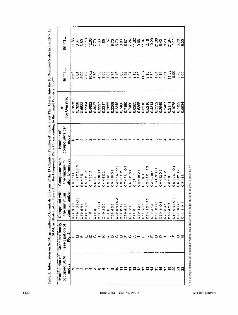
The optimal SOM grid size, which was found to be 10 � 10,classified the 325 compounds characterized by a 24-dimen-sional vector (the above 23 molecular descriptors plus thetarget variable ln��) into 80 nodes (neurons) of the map duringtraining, with an adequate population density, as illustrated bythe component plane for ln�� depicted in Figure 2. This figureidentifies 13 chemical families that cluster into the 80 nodeswith clustered compounds (occupied nodes) according to boththeir generic family label and molecular similarity. Gray levelsindicate the clustering compactness in each node, as measuredby the average distance (n) between the clustered compounds.Table 1 lists the main characteristics of the 80 occupied nodes,along with an indication on how compounds cluster into them,

according the molecular information provided by the 23 de-scriptors and the corresponding ln�� values.

A close inspection of Figure 2 and Table 1 reveals severalimportant features about the data set, molecular informationembedded in the molecular descriptors, and classification pro-cess, as listed below:

(1) The SOM captures the distinctiveness of the 13 chemicalfamilies (A–M) as characterized by the 23 molecular descrip-tors and the ln�� values, with a dominant presence in the nodesof clusters formed by the two most populated chemical familiesD (hydrocarbons with oxygen substituents) and E (halogenatedaliphatic hydrocarbons). The neighborhood between clusters isalso consistent with the formal segregation of the data set into13 chemical families A–M.

(2) Nearly 70% of the 80 occupied nodes (Figure 2) containcompounds of the same chemical family. The remaining 30%of the occupied nodes are formed by similar compounds fromother neighbor ones. For example, clusters (nodes) 40, 46, 49,58, and 59 are formed by chemicals from families C (aliphatichydrocarbons) and H (cyclic hydrocarbons).

(3) Nodes consistently cluster chemicals with similar struc-tures. However, there are significant differences between thedegree of membership by which nodes cluster chemicals and ofthe span of the corresponding ln�� values. This is clearlyobserved in Table 1, where the square of the cluster average

Figure 2. Distribution of 13 families of organic com-pounds over the component plane for ln��.(A) Monoaromatic hydrocarbons (20 compounds); (B) pol-yaromatic hydrocarbons (5 compounds); (C) aliphatic hydro-carbons (36 compounds); (D) hydrocarbons with oxygen sub-stituents (123 compounds); (E) halogenated aliphatichydrocarbons (66 compounds); (F) aromatic hydrocarbonswith nitrogen and/or oxygen substituents (11 compounds);(G) hydrocarbons with sulfur substituents and/or oxygenand/or nitrogen (19 compounds); (H) cyclic hydrocarbons (15compounds); (I) aromatic hydrocarbons with oxygen substitu-ents (8 compounds); (J) halogenated aromatic hydrocarbons(9 compounds); (K) heterocyclic hydrocarbons (10 com-pounds); (L) aliphatic hydrocarbons with halogen and oxygensubstituents (2 compounds); (M) aliphatic hydrocarbons withnitro and halogen groups (1 compound). The gray levelsindicate the clustering intensity of the ln�� data set into theSOM nodes measured by the average distance (n) betweenmembers of each cluster.


Tab

le1.

Info

rmat

ion

onSe

lf-O

rgan

izat

ion

ofC

hem

ical

sin

Ter

ms

ofth

e13

Che

mic

alF

amili

esof

the

Dat

aSe

tT

hat

Clu

ster

into

the

80O

ccup

ied

Nod

esin

the

10�

10SO

M,

asIl

lust

rate

din

Fig

ure

2fo

rth

eC

ompo

nent

Pla

neC

orre

spon

ding

toth

eT

arge

tP

rope

rty

ln�

�*

*The

aver

age

dist

ance

ofco

mpo

unds

with

inea

chcl

uste

rof

the

node

sin

the

U-m

atri

xis

give

nby

n2.


Tab

le1.

Info

rmat

ion

onSe

lf-O

rgan

izat

ion

ofC

hem

ical

sin

Ter

ms

ofth

e13

Che

mic

alF

amili

esof

the

Dat

aSe

tT

hat

Clu

ster

into

the

80O

ccup

ied

Nod

esin

the

10�

10SO

M,

asIl

lust

rate

din

Fig

ure

2fo

rth

eC

ompo

nent

Pla

neC

orre

spon

ding

toth

eT

arge

tP

rope

rty

ln�

�*

(Con

tinu

ed)


distance for each node in the U-matrix, (n2), and the corre-sponding minimum and maximum values of ln�� are listed forthe 80 occupied nodes. The span of ln�� is very noticeable andsignificant in the more populated clusters (number of com-pounds � 5) (that is, nodes 1, 9, 12, 14, 15, 24–28, 35–40, 46,47, 49–51, 63, and 67). It should be noted that ln�� is only onecomponent in the 24-dimensional vectors (23 descriptors plusln��) characterizing the nodes in the map. It is also well knownthat it is difficult to account for heteroatoms, particularly halo-gens, within any given chemical structure with molecular de-scriptors (Basak and Maguson, 1988; Carbo-Dorca and Besalu,1998). The dispersion (n2) of compounds around nodes inTable 1 clearly illustrates this difficulty. The dispersion ofcompounds is smallest (0.1093 � n2 � 0.2064) in the morepopulated nodes 37, 40, 46, and 50, which cluster only familiesof hydrocarbons with no substituents containing heteroatoms(families A, B, C, H, and K). This dispersion increases(0.0854 � n2 � 0.6353) in the populated nodes 9, 12, 15, 26,28, 36, 39, 47, 49, 51, 63, 67, 92, 94, 95, and 97 that clusterhydrocarbons with oxygen, nitrogen, and/or sulfur substituents(families D, F, G, and I). The largest dispersion (0.2155 � n2 �0.7828) is encountered in nodes 1, 14, 24, 25, 27, 35, and 91with hydrocarbon families with halogen substituents (E, J, L,and M).

Finally, it should be noted that the component plane for ln��

in Figure 2 is compact, given that three or more nodes withclustered compounds (occupied nodes) usually surround theempty ones, implying that the latter were also updated bymeans of Eqs. 2 and 3 during training. Thus, vectors of theempty nodes are bound to be a good source of additional(interpolated) information for training the QSAR models withthe aim at increasing generalization during testing or predictiveoperation mode, even at the expense of introducing some noisein the training set. In the current study, the 100 node vectors ofa 10 � 10 SOM, built only from information of the training set,were also used as additional information for training the fuzzy-ARTMAP–based QSPR model. In such a way, the interpolatedinformation obtained from this SOM may enhance the classi-fication capabilities of any new information presented to thepredictive fuzzy ARTMAP neural system during testing.

Selection of most suitable descriptors

The component planes of the 10 � 10 SOM, built frommolecular and target ln�� information of the complete set of325 compounds, were used to select the most suitable set ofmolecular descriptors from the initial pool of 23 topologicaland quantum chemical descriptors. The selection was carriedout according to the descriptors’ contribution to the classifica-tion of the 325 compounds in relation to ln�� and following themethodology of index selection proposed by Espinosa et al.(2002). Accordingly, the 23 component C-planes shown inFigure 3 are grouped into six classes according to the similarityin the contribution of descriptors to the topological organiza-tion of the map. The six classes, identified with the Romannumerals I–VI, were formed by curvilinear component analy-sis. A visual inspection of Figure 3 shows that the classificationinto six classes of similar descriptors is consistent with thesimilarity shown by their respective C-planes. The first threeclasses include the topological (connectivities, kappa index,and the sum of atomic numbers) and quantum informationT

able

1.In

form

atio

non

Self

-Org

aniz

atio

nof

Che

mic

als

inT

erm

sof

the

13C

hem

ical

Fam

ilies

ofth

eD

ata

Set

Tha

tC

lust

erin

toth

e80

Occ

upie

dN

odes

inth

e10

�10

SOM

,as

Illu

stra

ted

inF

igur

e2

for

the

Com

pone

ntP

lane

Cor

resp

ondi

ngto

the

Tar

get

Pro

pert

yln

��

*(C

onti

nued

)


(average polarizability, number of filled levels, and nuclear–nuclear repulsion). Because each of these classes containsdescriptors with 2-D molecular size–related information theyshould help to explain how the increase in chain length orhydrophobicity is related with ln��. The dipole moment isappropriately grouped in class IV with the Hansen indices,whereas the remaining atomic energies and all MQS matricesare classified into classes V and VI, respectively. The classifi-cation of C-planes shown in Figure 3 is also consistent with thecovariances between descriptors and target variable listed inTable 2. The highest covariance with ln�� corresponds to 1�v

(class I), whereas the first descriptor with a C-plane organiza-tion is significantly different from cluster I and with a still highcovariance, is (class IV). It is interesting to note that the useof these two descriptors proved to be very effective in the linearcorrelations of ln�� proposed by Medir and Giralt (1982) forhydrocarbons.

The ordering of indices, selected descriptors, and the basisfor the descriptors’ selection process are summarized in Table3. The first indices selected from the initial pool to form themost suitable set were those with highest absolute covariancewith ln�� in each of the six classes of Figure 3 (that is, 1�v, N,4�v, , ENA, and Cou). In this case, all six indices wereselected because their covariances are higher than the averagevalue for the whole pool of 23 descriptors, as may be deducedfrom the information provided in Table 2. As can be verifiedfrom Table 3, the successive addition of descriptors in theprocess of selecting the most suitable set causes a decrease inthe value of the dissimilarity function, defined by Eq. 6, from0.703 for 1�v to 0.229, when the six indices mentioned abovewere incorporated. This significant decrease highlights the im-portance of adding indices according to their topological im-pact on the studied QSPR. Further addition of 3�v, NFL, AP,2�v, and NNR, chosen according to their absolute covariancewith ln��, lowered the dissimilarity to the minimum value of0.190. It is important to recognize that molecular informationbeyond the point of minimum dissimilarity (Table 3) can beredundant, it may introduce noise if added to the QSPR, and itcould also induce errors attributed to conflicting informationwith the previous and more relevant indices of the most suit-able set. Values of the 11 descriptors, included in the mostsuitable set (constructed from the initial pool of descriptors),for the compounds in the overall data set, are provided in thesupporting information (see Table 5 below). The final set of themost suitable 11 descriptors identified in the present workincludes nine of the 11 descriptors used by Yaffe et al. (2001)to predict the aqueous solubility of organic compounds. Theseauthors used a nonlinear selection method, based on a dynamicbackpropagation neural network genetic algorithm, to identify11 suitable descriptors from an initial set of 30 descriptors. Inthe present set, the RE and EE descriptors used by Yaffe et al.(2001) were substituted here by Cou and N. Also, it is notedthat the current incorporation of the sum of atomic numbersreinforces the well-known dependency of ln�� with chainlength (Mackay and Shiu, 1977; Medir and Giralt, 1982).

To assess QSPR performance when solely using significantand coherent quantum chemical information, the above selec-tion procedure was also applied to the six MQS descriptors(Table 3), which constitute class VI shown in Figure 3. Twoclasses were identified, one formed by the three coulombdescriptors and the other including all overlap information. The

most suitable set, formed by Cou, CouC6H8, CouC3H7Cl, andOve, was selected based on the minimum average dissimilarityvalue. It is interesting to note that the Ove descriptor is neededdespite its low covariance with ln�� (see Table 2), which isbelow the average for the complete MQS set, given that it is theonly source of quantum information for molecular shape avail-able in this set of most suitable MQS matrices.

QSPR models

Fuzzy-ARTMAP–based QSPR for ln�� were developed us-ing either the most suitable set of 11 descriptors from the initialset listed in Table 3 [1�v, N, 4�v, , ENA, Cou, 3�v, NFL, AP,2�v, and NNR] or solely using the most significant MQS matrix[Cou, CouC6H8, CouC3H7Cl, and Ove]. In each case, training wascarried out by using either the training set of 280 compounds orthis subset complemented with the interpolated informationobtained from a 10 � 10 SOM, trained only with the moleculardescriptors of these 280 compounds and the target variableln��, as discussed previously.

The fuzzy-ARTMAP algorithm is a neural classifier andonly the presentation of new information during training willtrigger the creation of new classes in ARTb according to therequired accuracy for the target variable ln��, and correspond-ingly the creation of an equal or larger number of classes forthe training compounds in ARTa. This ensures the generationof many (compounds in ARTa) to one (ln�� value in ARTb)relationships in the network. The accuracy in ARTb is set by afixed vigilance parameter �b, whereas that of ARTa increasesdynamically from zero according to the needs of classificationand of the if–then relationships. Thus, overtraining in fuzzyARTMAP will manifest itself in the creation of an unneces-sarily large architecture (Georgiopoulos et al., 2001) and asdegradation in generalization capabilities of the predictivemodel (that is, poor performance on samples or data not presentin the training set).

In the current study the generation of a reasonable number ofclasses has been monitored and reasonable generalization en-sured by choosing a training set (Espinosa et al., 2001b) of 280compounds that was representative of the complete set of 325compounds. The alternative of applying cross-validation pro-cedures (Koufakou et al., 2001) during the training stage didnot yield significantly different results since the predictivecapabilities of the current model are very demanding, that is,the number of chemical families and the range of ln�� valuesare both very large. It should be noted that the current approachwould allow the construction of a nearly zero biased network(close to zero training error) that will also have good general-ization capabilities and yield a finite small variance for the testset. This is possible in the framework of the bias/variancedilemma (Geman et al., 1992) since any test data presented tothe network that are not well represented by the current trainingset (that is, test data not included in the current test set of 45compounds) would be labeled as “unable to classify” in ARTa

within the classification error tolerance and considered as anew candidate for training. Very large or infinite errors couldbe assumed for these hypothetical, unclassifiable test data sothat the product of the error of the training set times the errorof a test set, formed by the classifiable and unclassifiablecompounds, would still be finite. In addition, the use of SOMprototypes, for enhanced learning in a fuzzy-ARTMAP–based


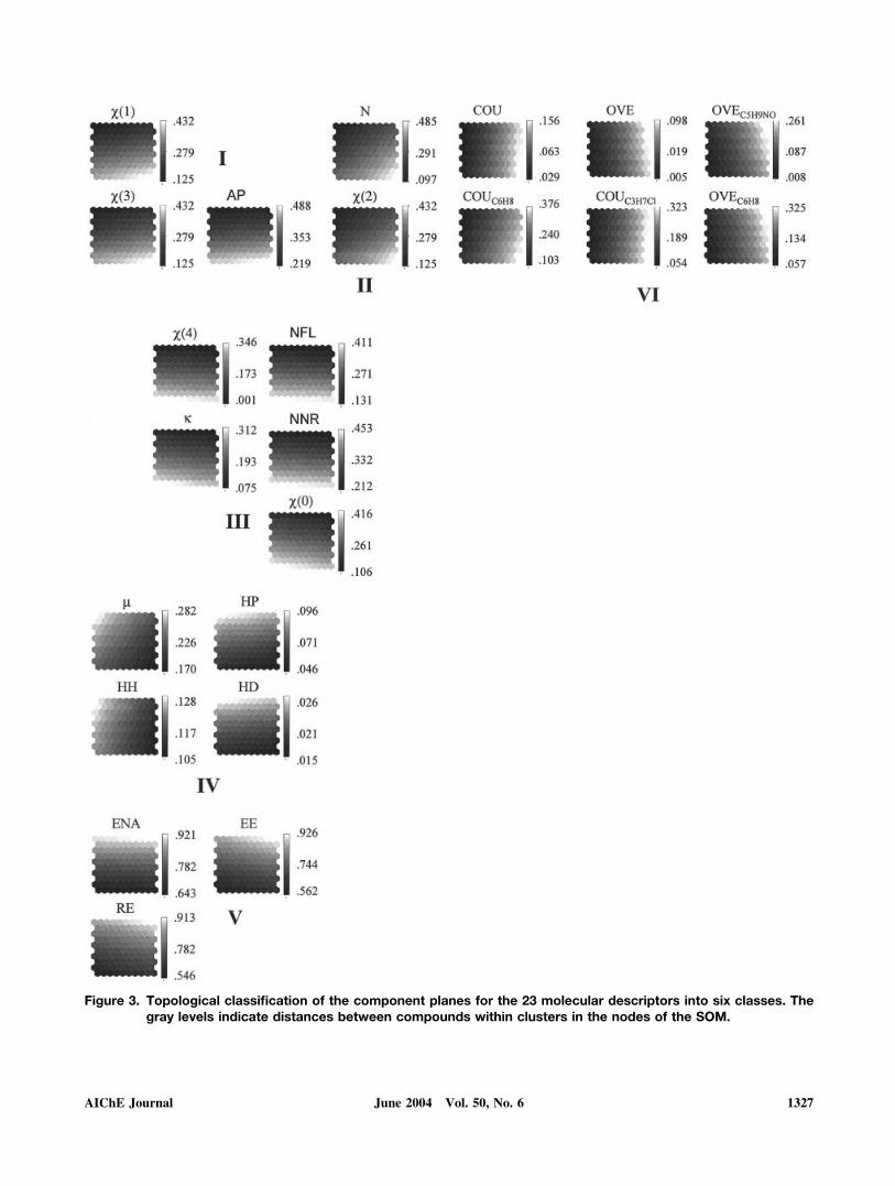
Figure 3. Topological classification of the component planes for the 23 molecular descriptors into six classes. Thegray levels indicate distances between compounds within clusters in the nodes of the SOM.


Tab

le2.

Cov

aria

nce

Mat

rix

for

the

23M

olec

ular

Des

crip

tors

,G

roup

edA

ccor

ding

toth

eC

lass

ifica

tion

ofF

igur

e3,

and

Exp

erim

enta

lIn

finit

yD

iluti

onA

ctiv

ity

Coe

ffici

ent,

ln�

�


model, does not imply weighted fitting of input data because atmost only a few extra classes in the ART modules will becreated during training. More information and discussions onstatistics and generalization in relation to neural networks canbe found elsewhere (Cheng and Titterington, 1994).

The performance of the fuzzy-ARTMAP–based QSPR withthe most suitable set of 11 descriptors is summarized in Figure4. This fuzzy-ARTMAP–based QSPR model performed withan average absolute error and standard deviation of 0.09(1.21%) and 0.29 (3.65%) ln�� units, respectively, for thecomplete set of 325 compounds. The remarkable generalizationcapability of this model is illustrated by the prediction of ln��

for the test set of 45 chemicals, as shown in Figure 4a, with anaverage absolute error and standard deviation of 0.52 (6.64%)and 0.51 (6.23%) ln�� units, respectively. The performance ofthe above QSPR for the training set of 280 compounds [Figure4(a)] was with a very low average absolute error and standarddeviation of 0.02 (0.36%) and 0.02 (0.60%) ln�� units, respec-tively. This high level of performance for the training set isexpected, given that fuzzy ARTMAP is a neural classifier. Infact, errors for the training set could ultimately be reduced tozero by increasing precision to the point where all fuzzyARTMAP classes are occupied each with a single compound.However, this would hinder or prevent predictive generaliza-tion during testing, which is the main goal of QSPR models.Thus, a vigilance parameter of 0.999 was used in the currentstudy as a compromise between adequate precision for trainingand reasonably accurate predictive generalization for the test-ing phase, as illustrated in Figure 4a.

The performance of the fuzzy ARTMAP QSPR with themost suitable set of descriptors was further increased upontraining using both the 100 prototypes (obtained from the SOM

analysis as described before) and the training set of 280 com-pounds. In this case of enhanced training, the vigilance param-eter of the ARTMAP algorithm was relaxed from 0.999 to0.995 to promote generalization in the testing, despite the likelyincrease in training errors that this strategy could cause. Theresulting QSPR performance for the test set was with averageabsolute error and standard deviation that decreased to 0.40(5.35%) and 0.48 (5.85%) ln�� units, respectively, relative tothe performance obtained without the prototypes [Figure 4b].We note that, as a consequence of this strategy of enhancinggeneralization during testing, the average absolute errors andstandard deviations when training with the prototypes in-creased to 0.05 (1.07%) and 0.04 (6.42%) ln�� units. Compar-ison of Figure 4(a) and (b) indicates that the inclusion ofprototypes in the training phase improves the classification of12 chemicals out of the 45 test set chemicals. This is so because11 of these chemicals were assigned during testing to fuzzyARTMAP classes formed by prototypes of occupied SOMnodes and one was assigned to a class formed by a prototype ofan empty but trained node, as indicated in Figure 4(b).

In addition to the above QSPRs, the four most suitable MQSmeasures alone (Cou, CouC6H8, CouC3H7Cl, and Ove) were usedto construct a QSPR using the same training set of 280 com-pounds. The performance of the resulting QSPR, for the test setof 45 compounds, was with an average absolute error andstandard deviation of 0.92 (11.2%) and 1.09 (11.5%) ln��

units, respectively. Although the above error and standarddeviation are approximately twice those obtained for the mostsuitable set of 11 indices (Figure 4), the performance is re-markable considering that only four MQS matrices were used.It is also interesting to note that the inclusion of the 100 SOMprototypes in the training phase did not improve the QSPR’s

Table 3. Initial Set of Descriptors, Covariances, and Cumulative Dissimilarity Measures Ordered According to the SOMVariable Selection Procedure

Descriptor Abbreviation ClassCovariance withTarget Variable

CumulativeDissimilarity

Valence connectivity index of first order 1�v I 0.632 0.703Sum of atomic numbers N II 0.583 0.553Valence connectivity index of fourth order 4�v III 0.553 0.366Dipole moment IV �0.535 0.276Electron–nuclear attraction ENA V �0.508 0.243Coulomb self-similarity Cou VI 0.425 0.229Valence connectivity index of the third order 3�v I 0.584 0.212Number of filled levels NFL II 0.543 0.204Average polarizability AP I 0.541 0.195Valence connectivity index of second order 2�v II 0.527 0.191Nuclear–nuclear repulsion energy NNR III 0.496 0.190Hansen polarizability HP IV �0.494 0.192Hansen hydrogen bonding HH IV �0.491 0.196Exchange energy EE V �0.451 0.198Resonance energy RE V �0.439 0.201Kappa second-order index 2� III 0.437 0.211Valence connectivity index of zero order 0�v III 0.435 0.218Molecular quantum cross-similarity of

Coulomb with respect to C6H8 CouC6H8 VI 0.419 0.234Molecular quantum cross-similarity of

Coulomb with respect to C3H7Cl1 CouC3H7Cl1 VI 0.334 0.253Overlap self-similarity Ove VI 0.170 0.257Molecular quantum cross-similarity of

Overlap with respect to C6H8 OveC6H8 VI 0.121 0.270Molecular quantum cross-similarity of

Overlap with respect to C5H9N1O1 OveC5H9N1O1 VI �0.037 0.377Hansen dispersivity HD IV �0.002 0.381


performance in this case, given that errors associated with thedescription halogen groups with only MQS matrices also prop-agate over the map and thus negate the increase in interpolationcapabilities. It is noted that the errors associated with hydro-

carbon families containing halogen substituents tend to be thelargest in Table 4.

To illustrate the potential of using MQSM as the fundamen-tal source of molecular information in QSPR building, anadditional model was developed with the set of four similaritymeasures mentioned above (Cou, CouC6H8, CouC3H7Cl, andOve), the sum of atomic numbers, and the sum of atomicsnumbers of heteroatoms, to better account for size effects andfor the presence of such atoms in the target molecules. Theperformance of the above QSPR, for the test set of 45 com-pounds, was with an average absolute error and standard de-viation of 0.57 (7.06%) and 0.57 (7.06%) ln�� units, respec-tively, a level of performance similar to that obtained with themost suitable set of 11 indices [Figure 4a].

It is instructive to explore the performance of the presentQSPRs for specific families of organic compounds, as illus-trated in Table 4. Clearly, the MQS-based model performs verywell when the training data set is large and the range ofmolecular sizes (that is, number of carbon atoms) is narrow.This is an indication of the need for more and/or improvedshape information than provided by the Overlap operator. It isnoted that the performance results given in Table 4, in terms ofthe average absolute errors and standard deviations, are for thecomplete data set (training plus test data); thus differencesbetween the different models are not as evident as with com-parisons based on the test set (such as Figures 4 and 5). Thischoice, however, facilitates comparison with previous studies,as discussed in the next section.

Comparison with previous studies

The current fuzzy ARTMAP models were compared withthe best performing neural network–based QSPR reported byMitchell and Jurs (1998) and with the regression-based QSPRof Medir and Giralt (1982) for specific chemical families. Themodel of Mitchell and Jurs (1998) is a multilayer perceptron,with an input–hidden-output layer architecture of 12–6–1units, respectively, trained with a quasi-Newton BFGS (Broy-den–Fletcher–Goldfarb–Shanno) algorithm. These authorsused 12 indices that included three topological descriptors, fourcharged partial surface area indices, two hydrogen bondingmeasures, the heat of formation, and two theoretical linearsolvation energy relationships. To consistently compare previ-ous and current models for the different chemical familiespresent in the data set of 325 compounds (Mitchell and Jurs,1998; Sherman et al., 1996), and to avoid the impedimentscaused by the different training and test sets used, the resultsare presented in Table 4 in terms of chemical families withoutdistinguishing training and test compounds. Also, the correla-tion reported by Medir and Giralt (1982) was recalculated foreach of the chemical families A, B, and C to adapt it to themore complete set of current data (Mitchell and Jurs, 1998;Sherman et al., 1996).

The performance of the present fuzzy-ARTMAP–basedQSPR model was better than the neural network model ofMitchell and Jurs (1998) for each of the 13 homogeneousfamilies present in the data set of 325 compounds (Table 4).The current two models, developed with the most suitable setof descriptors and trained by either the training set of 280compounds or by these compounds with the 100 prototypesfrom the SOM, performed with absolute mean errors and

Figure 4. Comparison between experimental ln�� val-ues and those predicted with the two currentfuzzy ARTMAP models developed using themost suitable set of eleven descriptors andtrained with (a) 280 compounds or (b) 280 com-pounds complemented with 100 prototypes ofclustered compound in the SOM nodes.Note that (b) depicts results only for the test data set of 45compounds.


Figure 5. Comparison between experimental ln�� values and those predicted with the current fuzzy ARTMAP modeldeveloped using only the most suitable set of four MQSM and trained with 280 compounds.

Table 4. Comparison of Performances of Current and Previous QSPR Models in Terms of Absolute Mean Error (StandardDeviation) in the Prediction of ln�� for the 13 Families of Organic Compounds Included in the Data Set

ID FamilyNumber ofCompounds

Number ofCarbonAtoms

FuzzyARTMAPBest Set

FuzzyARTMAP

MQSM

Fuzzy ARTMAPBest Sets and

SOM Prototypes

12–6–1 NN(*)

(Mitchell andJurs10)

Medir andGiralt9

A Monoaraomatic hydrocarbons 21 C6–C10 0.22 (0.57) 0.53 (1.34) 0.07 (0.15) 0.54 (1.13) 0.56 (1.09)(1)

B Polyaromatic hydrocarbons 5 C9–C12 0.07 (0.10) 0.16 (0.38) 0.06 (0.10) 0.22 (0.28) 0.30 (0.15)(2)

C Aliphatic hydrocarbons 35 C4–C8 0.10 (0.25) 0.32 (0.75) 0.15 (0.38) 0.45 (0.47) 0.46 (0.32)(3)

DHydrocarbons with oxygen

substituents 124 C1–C18 0.06 (0.17) 0.09 (0.31) 0.09 (0.18) 0.70 (0.78) —E Halogenated aliphatic hydrocarbons 66 C1–C6 0.12 (0.34) 0.12 (0.43) 0.12 (0.27) 0.82 (2.25) —

F

Aromatic hydrocarbons withnitrogen and/or oxygensubstituents 16 C5–C8 0.05 (0.12) 0.06 (0.20) 0.06 (0.06) 1.12 (2.11) —

G

Hydrocarbons with sulfursubstituents and/or oxygen and/ornitrogen 19 C1–C4 0.09 (0.14) 0.26 (0.61) 0.10 (0.16) 0.18 (0.12) —

H Cyclic hydrocarbons 15 C5–C9 0.07 (0.17) 0.10 (0.34) 0.10 (0.19) 0.51 (0.52) —

IAromatic hydrocarbons with oxygen

substituents 8 C7–C8 0.04 (0.03) 0.03 (0.03) 0.03 (0.04) 0.25 (0.23) —J Halogenated aromatic hydrocarbons 9 C6–C7 0.01 (0.02) 0.06 (0.12) 0.07 (0.05) 0.27 (0.24) —K Heterocyclic hydrocarbons 5 C4–C8 0.02 (0.03) 0.00 (0.00) 0.03 (0.04) 0.36 (0.25) —

LAliphatic hydrocarbons with

halogen and oxygen substituents 2 C2–C4 1.41 (1.99) 1.00 (1.42) 0.10 (0.05) 0.15 (0.11) —

MAliphatic hydrocarbons with nitro

and halogen groups 1 C1 0.01 (0.00) 0.01 (0.00) 0.06 (0.00) 0.08 (0.00) —

*The performance of this model by families was not reported in the original reference. The values included in this table have been currently calculated with the original12–6–1 feedforward architecture.

(1)ln�� 2.99 2.58 1�v.(2)ln�� 0.054 3.1 1�v.(3)ln�� 5.461 2.739 1�v 5.884 .


standard deviations that are on the average seven times smallerthan errors obtained with the model of Mitchell and Jurs(1998). Improved QSPR performance is also noted relative tothe linear regression models of Medir and Giralt (1982). It isinteresting to note that, for the two families of aromatic hydro-carbons A and B, this linear model with only the first-orderconnectivity as descriptor yields comparable predictions tothose obtained with the model of Mitchell and Jurs (1998)calculated for the whole data set. In the case of aliphatichydrocarbons (family C) the dipole moment was also includedin the linear correlation to maintain performance.

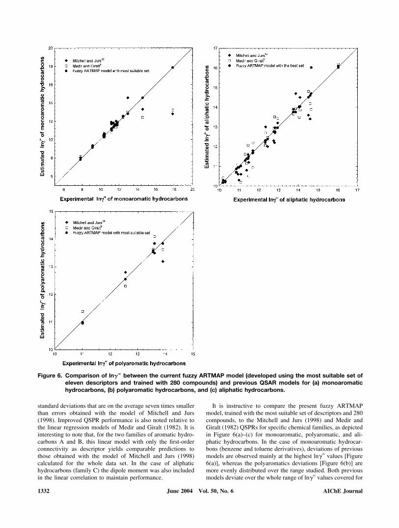
It is instructive to compare the present fuzzy ARTMAPmodel, trained with the most suitable set of descriptors and 280compounds, to the Mitchell and Jurs (1998) and Medir andGiralt (1982) QSPRs for specific chemical families, as depictedin Figure 6(a)–(c) for monoaromatic, polyaromatic, and ali-phatic hydrocarbons. In the case of monoaromatic hydrocar-bons (benzene and toluene derivatives), deviations of previousmodels are observed mainly at the highest ln�� values [Figure6(a)], whereas the polyaromatics deviations [Figure 6(b)] aremore evenly distributed over the range studied. Both previousmodels deviate over the whole range of ln�� values covered for

Figure 6. Comparison of ln�� between the current fuzzy ARTMAP model (developed using the most suitable set ofeleven descriptors and trained with 280 compounds) and previous QSAR models for (a) monoaromatichydrocarbons, (b) polyaromatic hydrocarbons, and (c) aliphatic hydrocarbons.


Tab

le5.

Mol

ecul

arD

escr

ipto

rsan

dE

xper

imen

tal

Aqu

eous

Infin

ity

Dilu

tion

Act

ivit

yC

oeffi

cien

tsfo

rth

eD

ata

Set

of32

5O

rgan

icC

ompo

unds

*

*(1–

4) �

v�

vale

nce

conn

ectiv

ityin

dex;

N�

sum

ofat

omic

num

bers

;N

FL

�nu

mbe

rof

fille

dle

vels

;

�di

pole

mom

ent;

AP

�av

erag

epo

lari

zabi

lity

(PM

3);

EN

A�

elec

tron

–nuc

lear

attr

actio

n;N

NR

�nu

clea

r–nu

clea

rre

puls

ion;

Cou

(Cou

lom

bM

QS)

.


Tab

le5.

Mol

ecul

arD

escr

ipto

rsan

dE

xper

imen

tal

Aqu

eous

Infin

ity

Dilu

tion

Act

ivit

yC

oeffi

cien

tsfo

rth

eD

ata

Set

of32

5O

rgan

icC

ompo

unds

*(C

onti

nued

)


aliphatic hydrocarbons, with greater scatter in the Mitchell andJurs (1998) model. The current “best” model performed rea-sonably well over the entire data range covered except for theoutlier 1-octene.

Conclusions

The integration of self-organizing maps (SOMs) with afuzzy ARTMAP neural system was applied to develop QSPRsfor the aqueous infinite dilution activity coefficient of organiccompounds based in a heterogeneous data set of 325 organiccompounds. The present study demonstrated that SOMs can beeffectively used to classify organic chemicals according to theirstructural information (that is, in terms of molecular descrip-tors). A SOM-based analysis was shown to be effective forselecting the most suitable set of descriptors from an initial set,and for generating complementary interpolated input informa-tion for training. The QSPRs developed for ln�� performedwith remarkable predictive generalization capabilities.

The fuzzy-ARTMAP–based QSPR developed with 11 de-scriptors, based on the data set of 325 compounds, performedwith average absolute errors of 0.02 (0.36%) and 0.52 (6.64%)ln�� units, for the training and test sets, respectively. Thisperformance was superior to that of other QSPRs reported inthe literature. When the prototypes were added to the trainingset, the average absolute error slightly increased to 0.05(1.07%) ln�� units and for the training set and decreased to0.40 (5.36%) ln�� units for the test set. The performance of theln�� QSPR, based only on four molecular quantum similaritymeasures, also selected by means of SOMs from a limited poolof six similarity measures, was better than that of previousQSPR models, with average absolute errors of 0.02 (0.38%)and 0.92 (11.2%) ln�� units for the training and test sets,respectively. The present results suggest that it should bepossible to develop accurate QSPRs using the informationcontained in the quantum similarity matrices. Such an ap-proach, however, will require improvements in the calculationof the quantum atomic density functions of molecules withheteroatoms using the metrics given by different quantumoperators.

Although the present study focused on the aqueous infinitedilution activity coefficient as a case study, the present ap-proach of using SOM analysis for features extraction, in com-bination with the modified fuzzy-ARTMAP classifier for vari-able prediction, could be an effective tool in various chemicalengineering applications for the identification of critical (orsignificant) variables or parameters, pattern recognition, andestablishing parameter–property relations.

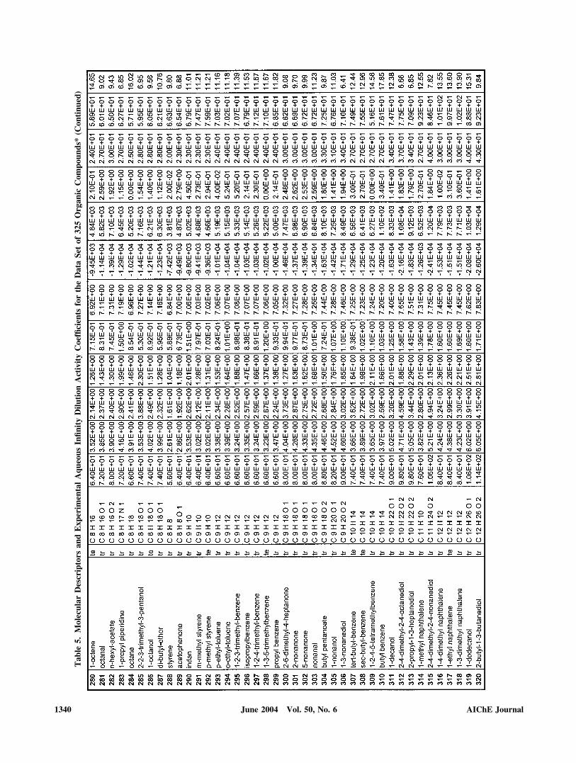
Available supporting information

We provide Table 5 as supplemental, supporting data, listingthe best set of molecular descriptors and the experimentalinfinity dilution activity coefficients for the 325 organic com-pounds considered.

AcknowledgmentsThe authors are grateful for the financial support received from the

“Direccion General de Investigacion Cientıfica y Tecnica,” ProjectsPPQ2000-1339 and PPQ2001-1519, and from the CIRIT “Programa deGrups de Recerca Consolidats de la Generalitat de Catalunya,” Projects1998SGR-00102 and 2000SGR-00103.

Tab

le5.

Mol

ecul

arD

escr

ipto

rsan

dE

xper

imen

tal

Aqu

eous

Infin

ity

Dilu

tion

Act

ivit

yC

oeffi

cien

tsfo

rth

eD

ata

Set

of32

5O

rgan

icC

ompo

unds

*(C

onti

nued

)


Literature CitedAgrawal, T., T. Imielinsky, and A. Swami, “Database Mining: A Perfor-

mance Perspective,” IEEE Trans. Knowl. Data Eng., 5, 6 (1993).Amat, L., and R. Carbo-Dorca, “Quantum Similarity Measures under

Atomic Shell Approximation: First Order Density Fitting Using Elemen-tary Jacobi Rotations,” J. Comput. Chem., 18, 2023 (1997).

Amat, L., R. Carbo-Dorca, and R. Ponec, “Simple Linear QSAR ModelsBased on Quantum Similarity Measures,” J. Med. Chem., 42, 5169(1999).

Amat, L., D. Robert, E. Besalu, and R. Carbo-Dorca, “Molecular QuantumSimilarity Measures Tuned 3D QSAR: An Antitumoral Family Valida-tion Study,” J. Chem. Inf. Comput. Sci., 38, 624 (1998).

Basak, S., and V. Maguson, “Determining Structural Similarity of Chem-icals Using Graph Theoretic Indices,” Discrete Appl. Math., 19, 17(1988).

Bishop, C. M., Neural Networks for Pattern Recognition, Oxford Univ.Press, Oxford, UK (1995).

Bunz, P., B. Braun, and R. Janowsky, “Application of Quantitative Struc-ture-Performance Relationship and Neural Network Models for thePrediction of Physical Properties from Molecular Structure,” Ind. Eng.Chem. Res., 37, 3043 (1998).

Carbo-Dorca, R., and E. Besalu, “A General Survey of Molecular QuantumSimilarity,” Theor. Chem., 45, 11 (1998).

Carpenter, G., and S. Grossberg, “A Massively Parallel Architecture for aSelf-Organizing Neural Pattern Recognition Machine.” Comput. Vis.Graphics Image Process., 37, 54 (1987).

Carpenter, G., S. Grossberg, N. Marcuzon, J. Reynolds, and D. Rosen,“Fuzzy ARTMAP: A Neural Network Architecture for IncrementalSupervised Learning of Analog Multidimensional Maps,” IEEE Trans.Neural Networks, 3, 698 (1992).

Carpenter, G., S. Grossberg, N. Marcuzon, and D. B. Rosen, “Fuzzy ART:Fast Stable Learning and Categorization of Analog Patterns by anAdaptive Resonance System,” Neural Networks, 4, 759 (1991).

Cheng, B., and D. M. Titterington, “Neural Networks: A Review from aStatistical Perspective,” Stat. Sci., 9(1), 2 (1994).

Chow, H., H. Chen, T. Ng, P. Myrdal, and S. H. Yalkowsky, “UsingBackpropagation Networks for the Estimation of Aqueous ActivityCoefficients of Aromatic Organic Compounds,” J. Chem. Inf. Comput.Sci., 35, 723 (1995).

Cramer, R., D. Patterson, and J. Bunce, “Comparative Molecular FieldAnalysis (CoMFA). 1. Effect of Shape on Binding of Steroids to CarriedProteins,” J. Am. Chem. Soc., 110(18), 5959 (1988).

Cybenko, G., “Approximation by Superposition of Sigmoidal Functions,”Math. Control Signal Syst., 2, 303 (1989).

Egolf, L., and P. Jurs, “Prediction of Boiling Points of Organic Heterocy-clic Compounds Using Regression and Neural Network Techniques,”J. Chem. Inf. Comput. Sci., 33, 616 (1993).

Erwing, E., K. Obermayer, and K. Schulten, “Self-Organizing Maps:Stationary States, Metastability and Convergence Rate,” Biol. Cybern.,67(1), 35 (1992).

Espinosa, G., A. Arenas, and F. Giralt, “Prediction of Boiling Points ofOrganic Compounds from Molecular Descriptors by Using Backpropa-gation Neural Networks,” in Fundamentals of Molecular Similarity, R.Carbo-Dorca, ed., Kluwer Academic, Dordrecht, 1 (2001a).

Espinosa, G., A. Arenas, and F. Giralt, “Integrated SOM-Fuzzy ARTMAPNeural System for the Evaluation of Toxicity,” J. Chem. Inf. Comput.Sci., 42(2), 343 (2002).

Espinosa, G., A. Arenas, and F. Giralt, “QSAR for TD50 of AromaticCompounds by Using an Integrated SOM-Fuzzy ARTMAP Based Neu-ral System with Topological and Quantum Molecular Similarity De-scriptors,” in Fundamentals of Molecular Similarity (V Girona Seminaron Molecular Similarity, Girona, Spain), Kluwer Academic, Dordrecht,The Netherlands (2003).

Espinosa, G., D. Yaffe, A. Arenas, Y. Cohen, and F. Giralt, “A FuzzyARTMAP Based on Quantitative Structure-Property Relationships(QSPRs) for Predicting Physical Properties of Organic Compounds,”Ind. Eng. Chem. Res., 40(12), 2757 (2001b).

Espinosa, G., D. Yaffe, Y. Cohen, A. Arenas, and F. Giralt, “NeuralNetwork Based Quantitative Structural Property Relations (QSPRs) forPredicting Boiling Points of Aliphatic Hydrocarbons,” J. Chem. Inf.Comput. Sci., 40, 859 (2000).

Fayyad, U. M., “Data Mining and Knowledge Discovery: Making SenseOut of Data,” IEEE Expert, 20 (1996).

Ferre-Gine, J., R. Rallo, A. Arenas, and F. Giralt, “Identification ofCoherent Structures in Turbulent Shear Flows with a Fuzzy ARTMAPNeural Network,” Int. J. Neural Syst., 7(5), 559 (1996).

Fessant, F., S. Bengio, and D. Collobert, “Use of Modular Architectures forTime Series Prediction,” Neural Proc. Lett. (1995).

Fredenslund, A., R. Jone, and J. Prausnitz, “Group-Contribution Estima-tion of Activity Coefficients in Nonideal Liquid Mixtures,” AIChE J.,21(6), 1086 (1975).

Gakh, A., E. Gakh, B. Sumpter, and D. Noid, “Neural Network-GraphTheory Approach to the Prediction of the Physical Properties of OrganicCompounds,” J. Chem. Inf. Comput. Sci., 34, 832 (1994).

Gasteiger, J., X. Li, C. Rudolph, J. Sadowski, and J. Zupan, “Representa-tion of Molecular Electrostatic Potentials by Topological Feature Maps,”J. Am. Chem. Soc., 116, 4608 (1994a).

Gasteiger, J., X. Li, and A. Uschold, “The Beauty of Molecular Surfaces asRevealed by Self-Organizing Neural Networks,” J. Mol. Graphics, 12,90 (1994b).

Geman, S., E. Bienenstock, and R. Doursal, “Neural Networks and theBias/Variance Dilemma,” Neural Comput., 4, 1 (1992).

Georgiopoulos, M., A. Koufakou, G. C. Anagnostopoulos, and T. Kasparis,“Overtraining in Fuzzy ARTMAP: Myth or Reality?” Proceedings of theIEEE-INNS-ENNS International Joint Conference on Neural Networks(IJCNN ’01), 2, 1186 (2001).

Giralt, F., A. Arenas, J. Ferre-Gine, R. Rallo, and G. A. Kopp, “TheSimulation and Interpretation of Turbulence with a Cognitive NeuralSystem,” Physics of Fluids, 12(7), 1826 (2000).

Gutfreund, H., and M. Mezard, “Processing of Temporal Sequences inNeural Networks,” Phys. Rev. Lett., 61, 235 (1988).

Hall, L., and C. Story, “Boiling Point and Critical Temperature of aHeterogeneous Data Set: QSAR Atom Type Electrotopological StateIndices Using Artificial Neural Networks,” J. Chem. Inf. Comput. Sci.,36, 1004 (1996).

Hansen, C. M., “The Three Dimensional Solubility Parameter—Key toPaint Component Affinities. II. Dyes, Emulsifiers, Mutual Solubility andCompatibility, and Pigments,” J. Paint Technol., 39, 509 (1979).

Hecht-Nielsen, R., “Replicator Neural Networks for Universal OptimalSource Coding,” Science, 269, 186 (1995).

Hertz, J., A. Krogh, and R. G. Palmer, Introduction to the Theory of NeuralComputation, Addison–Wesley, Reading, MA (1991).

Hornik, K., M. Stinchcombe, and H. White, “Multilayer FeedforwardNetworks are Universal Approximators,” Neural Networks, 2, 359(1989).

Karelson, M., V. Lobanov, and A. Katritzky, “Quantum-Chemical Descrip-tors in QSAR/QSPR Studies,” Chem. Rev., 96, 1027 (1996).

Kaski, S., and T. Kohonen, “Winner-Take-All Networks for PhysiologicalModels of Competitive Learning,” Neural Networks, 7, 973 (1994).

Kaski, S., and K. Lagus, “Comparing Self-Organizing Maps,” Proc. ofICANN’96, 809 (1996).

Kier, L., and L. Hall, Molecular Connectivity in Chemistry and DrugResearch, Academic Press, New York (1976).

Kier, L., and L. Hall, Molecular Connectivity in Structure–Activity Anal-ysis, Wiley, New York (1985).

Kier, L. B., and L. H. Hall, Molecular Structure Description: The Elect-rotopological State, Academic Press, Orlando, FL (1999).

Kohonen, T., “Self-Organizing Formation of Topologically Correct Fea-ture Maps,” Biol. Cybern., 43, 59 (1982).

Kohonen, T., “The Self-Organizing Map,” Proc. IEEE, 78, 1464 (1990).Koufakou, A., M. Georgiopoulos, G. Anagnostopoulos, and T. Kasparis,

“Cross-Validation in Fuzzy ARTMAP for Large Databases,” NeuralNetworks, 14, 1279 (2001).

Lazaridis, T., and M. Paulaitis, “Activity Coefficients in Dilute AqueousSolutions from Free Energy Simulations,” AIChE J., 39(6), 1051 (1993).

Mackay, D., W. Y. Shiu, and K. Ch. Ma, Illustrated Handbook of PhysicalChemical Properties and Environmental Fate for Organic Chemicals,Vol. 1, Lewis Publishers, Chelsea, MI (1992)

Mackay, D., and Y. Shiu, “Aqueous Solubility of Polynuclear AromaticHydrocarbons,” J. Chem. Eng. Data., 22, 399 (1977).

McWeeny, R., Methods of Molecular Quantum Mechanics, AcademicPress, New York (1989).

Medir, M., and F. Giralt, “Correlation of Activity Coefficients of Hydro-carbons in Water at Infinite Dilution with Molecular Parameters,” AIChEJ., 28(2), 341 (1982).

Mitchell, B., and P. Jurs, “Prediction of Infinite Dilution Activity Coeffi-


cients of Organic Compounds in Aqueous Solution from MolecularStructure,” J. Chem. Inf. Comput. Sci., 38, 200 (1998).

Molecular Modeling Pro™, Revision 3.1, ChemSM™ Inc. (1998).Peterson, D. L., and S. H. Yalkowsky, “Comparison of Two Methods for

Predicting Aqueous Solubility,” J. Chem. Inf. Comput. Sci., 41, 1531(2001).

Rallo, R., A. Arenas, J. Ferre-Gine, and F. Giralt, “A Neural Virtual Sensorfor the Inferential Prediction of Product Quality from Process Vari-ables,” Comput. Chem. Eng., 26(12), 1735 (2002a).

Rallo, R., J. Ferre-Gine, A. Arenas, and F. Giralt, “Forecasting ProductQuality in Industrial Processes with Virtual Sensors,” Proceedings of theTopical Conference on Sensor Technology, C. C. Liu, H. B. Martin, andJ. C. Angus, eds., AIChE Annual Meeting, AIChE Pub. No. P-172, 127(2002b).

Ran, Y., N. Jain, and S. H. Yalkowsky, “Prediction of Aqueous Solubilityof Organic Compounds by the General Solubility Equation (GSE),”J. Chem. Inf. Comput. Sci., 41, 1208 (2001).

Ran, Y., and S. H. Yalkowsky, “Prediction of Drug Solubility by theGeneral Solubility Equation (GSE),” J. Chem. Inf. Comput. Sci., 41, 354(2001).

Randic, M., “On Characterization of Molecular Branching,” J. Am. Chem.Soc., 97, 6609 (1975).

Randic, M., and N. Trinajstic, “Comparative Structure–Property Studies:The Connectivity Basis,” J. Mol. Struct., 284, 209 (1993).

Rani, Y. K., and N. V. K. Dutt, “Estimation of Activity Coefficients atInfinite Dilution of Halocarbons in Water and Organic Compounds inHydrofluoroparaffins Using Neural Networks,” Chem. Eng. Commun.,189(3), 372 (2002).

Sandler, S. I., “Quantum Mechanics: The New Engineering Thermody-namics,” Proceedings of the AspenWorld 2002, Washington, DC, Oct.–Nov. 2002 (https://www.aspenworld2002.com/).

Sherman, S. R., D. B. Trampe, D. M. Bush, M. Schiller, C. A. Eckert, A. J.Dallas, J. Li, and P. W. Carr, “Compilation and Correlation of LimitingActivity Coefficients of Nonelectrolytes in Water,” Ind. Eng. Chem.Res., 35, 1044 (1996).

Simamora, P., A. Miller, and S. Yalkowsky, “Melting Point and NormalBoiling Point Correlations: Applications to Rigid Aromatic Com-pounds,” J. Chem. Inf. Comput. Sci., 33, 437 (1993).

Stanton, D., L. Egolf, P. Jurs, and M. Hicks, “Computer-Assisted Predic-tion of Normal Boiling Points of Furans, Tetrahydrofurans and Thio-phenes,” J. Chem. Inf. Comput. Sci., 31, 301 (1991).

Stanton, D., L. Egolf, P. Jurs, and M. Hicks, “Computer-Assisted Predic-tion of Normal Boiling Points of Pyrans and Pyrroles,” J. Chem. Inf.Comput. Sci., 32, 306 (1992).

Stanton, D., and P. Jurs, “Development and Use of Charged Partial SurfaceArea Structural Descriptors for Quantitative Structural-Property Rela-tionship Studies,” Anal. Chem., 62, 2323 (1990).

Tochigi, K., D. Tiegs, J. Gmehling, and K. Kojima, “Determination of NewASOG Parameters,” J. Chem. Eng. Jpn., 23, 453 (1990).

Vesanto, J., “SOM-Based Data Visualization Methods,” Intell. Data Anal.,6, 111 (1999).

Viswanadhan, W., G. Mueller, S. Basak, and J. Weinstein, “Comparison ofa Neural Net-Based QSAR Algorithm (PCANN) with Hologram andMultiple Linear Regression-Based QSAR Approaches: Application to1-4-Dihydropyridine-Based Calcium Channel Antogonist,” J. Chem. Inf.Comput. Sci., 41, 505 (2001).

Voutsas, E. C., and D. P. Tassios, “Prediction of Infinite-Dilution ActivityCoefficients in Binary Mixtures with UNIFAC. A Critical Evaluation,”Ind. Eng. Chem. Res., 35, 1438 (1996).

Voutsas, E. C., and D. P. Tassios, “Analysis of the UNIFAC-Type GroupContribution Models at the Highly Dilute region. 1. Limitations of theCombinatorial and Residual Expressions,” Ind. Eng. Chem. Res., 36,4965 (1997).

Wiener, H., “Structural Determination of Paraffin Boiling Points,” J. Am.Chem. Soc., 69, 17 (1947).

Yaffe, D., Y. Cohen, G. Espinosa, A. Arenas, and F. Giralt, “A FuzzyARTMAP Based Quantitative Structure-Property Relationships(QSPRs) for Predicting Aqueous Solubility of Organic Compounds,”J. Chem. Inf. Comput. Sci., 41(5), 1150 (2001).

Yaffe, D., Y. Cohen, G. Espinosa, A. Arenas, and F. Giralt, “A FuzzyARTMAP Based Quantitative Structure-Property Relationships(QSPRs) for the Henry’s Law Constant of Organic Compounds,”J. Chem. Inf. Comput. Sci., 43(1), 85 (2003).

Yalkwosky, S., and S. Valvani, “Solubilities and Partitioning. 2. Relation-ship between Aqueous Solubilities, Partition Coefficients, and MolecularSurface Areas of Rigid Aromatic Hydrocarbons,” J. Chem. Eng. Data,24(2), 127 (1979).

Yalkowsky, S. H., Solubility and Solubilization in Aqueous Media, Amer-ican Chemical Society, Oxford, UK (1999).

Yalkowsky, S. H., and Y. He, Handbook of Aqueous Solubility Data, CRCPress, Boca Raton, FL (2003).

Yang, G., Y. Ran, and S. H. Yalkowsky, “Prediction of the AqueousSolubility: Comparison of the General Solubility Equation and theMethod Using an Amended Solvation Energy Relationship,” J. Pharm.Sci., 91, 517 (2002).

Manuscript received Jan. 2, 2002, revision received July 7, 2003, and final revisionreceived Sept. 13, 2003.


estimation of inﬁnite dilution activity coefﬁcients of...

Documents