estimation of in-situ petrophysical properties from ... · relative permeability capillary pressure...

Journal of Petroleum Science and Engineering 63 (2008) 1–17

Contents lists available at ScienceDirect

Journal of Petroleum Science and Engineering

j ourna l homepage: www.e lsev ie r.com/ locate /pet ro l

Estimation of in-situ petrophysical properties from wireline formation tester andinduction logging measurements: A joint inversion approach

Faruk O. Alpak a,⁎, Carlos Torres-Verdín a, Tarek M. Habashy b

a Department of Petroleum and Geosystems Engineering, The University of Texas at Austin, United Statesb Schlumberger-Doll Research, United States

⁎ Corresponding author. Now with Shell InternationaE-mail address: [email protected] (F.O. Alpak).

0920-4105/$ – see front matter © 2008 Elsevier B.V. Aldoi:10.1016/j.petrol.2008.05.007

a b s t r a c t
a r t i c l e i n f o
Article history:
We introduce a novel inver Received 2 April 2007Accepted 25 May 2008
Keywords:inverse problemspetrophysicsrelative permeabilitycapillary pressurewireline formation testinginduction logging

sion algorithm for the in-situ petrophysical evaluation of hydrocarbon-bearingformations. The algorithm simultaneously honors a set of multi-physics data: (a) Pressure-transient, flowlinefractional flow, and salt production rate measurements as a function of time acquired with a wireline-conveyed, dual-packer formation tester, and (b) borehole array induction measurements. Both time evolutionand spatial distribution of fluid saturation and salt concentration in the near-borehole region are constrainedby the physics of mud-filtrate invasion. The inverse problem consists of the simultaneous estimation of thenear-borehole permeability and parametric saturation functions of relative permeability and capillarypressure. A two-dimensional axisymmetric petrophysical model is assumed for the near-borehole region.Both horizontal and vertical permeabilities are subject to inversion. Saturation functions of relativepermeability and capillary pressure are parametrically represented using a modified Brooks–Corey model.We simulate the response of borehole logging instruments by reproducing the multi-phase, multi-component flow that takes place during mud-filtrate invasion and formation test. A fully implicit finite-difference black-oil reservoir simulator with brine tracking extension is used to simulate fluid-flowphenomena. Induction measurements are coupled to the physics of fluid flow using a rapid integro-differential algorithm. Inversion experiments consider both noise-free and noise-contaminated syntheticdata. Joint inversion results provide a quantitative proof-of-concept for the simultaneous estimation oftransversely anisotropic spatial distributions of permeability and saturation-dependent functions. Thestability and reliability of the inversions are conditioned by the accuracy of the a priori information aboutthe formation porosity and fluid PVT properties. We develop an alternative sequential inversion techniquefor cases where multi-physics measurements lack the degrees of freedom necessary to accurately estimateall the petrophysical model parameters. The first step involves estimation of horizontal and verticalpermeabilities from late-time transient-pressure measurements. Subsequently, the entire set of measure-ments is jointly inverted to yield saturation-dependent functions.

© 2008 Elsevier B.V. All rights reserved.

1. Introduction

The physics of multi-phase fluid-flow and electromagnetic induc-tion phenomena in porous media can be coupled through fluidsaturation equations. Thus, a multi-physics inversion algorithm for thequantitative joint interpretation of electrical and fluid-flow measure-ments can be formulated to estimate the underlying petrophysicalmodel.

1.1. Literature review

The dynamic properties of mud-filtrate invasion phenomena formthe basis for quantitative petrophysical interpretation of electricalconductivity profiles around the borehole. In the past, forward multi-

l E&P Inc.

l rights reserved.

physics algorithms/workflows were developed to perform sensitivitystudies. Examples can be found in Ramakrishnan and Wilkinson(1997), Zhang et al. (1999), Alpak et al. (2003), Li and Shen (2003), andGeorge et al. (2004). Inverse algorithms that make use of a multi-physics formulation have been introduced by Tobola and Holditch(1991), Yao and Holditch (1996), Semmelbeck et al. (1995), Ramak-rishnan et al. (1997), Ramakrishnan and Wilkinson (1999), Epov et al.(2002), Wu et al. (2002), Wu et al. (2003), Zeybek et al. (2004), andAlpak et al. (2004).

1.2. Problem statement

The objective of the work reported in this paper is to develop arobust, accurate, and efficient algorithm for the simultaneous,parametric joint inversion of magnetic field, transient-pressure,flowline water-cut, and salt production rate measurements. Theinversion algorithm yields two-phase flow petrophysical properties,

mailto:[email protected]

http://dx.doi.org/10.1016/j.petrol.2008.05.007

http://www.sciencedirect.com/science/journal/09204105

2 F.O. Alpak et al. / Journal of Petroleum Science and Engineering 63 (2008) 1–17

namely, layer-by-layer horizontal and vertical absolute permeabilities,parametric representations of relative permeability and capillarypressure curves, and initial phase saturations of the hydrocarbon-bearing rock formations. Although the algorithm can handle multi-layer cases, the proof-of-concept tests of this work were carried outfor the single-layer case. We assume standard instrument geometriesrather than proposing an experimental tool. However, we also explorethe possibility of taking a first step toward the future of the jointinterpretation of wireline formation tester (WFT) and inductionlogging (IL) measurements by introducing multi-pulse schedules forWFT measurements. We develop an alternative sequential inversiontechnique for cases where multi-physics measurements lack thedegrees of freedom necessary to accurately estimate all of thepetrophysical model parameters. We first resort to the single-phaseinversion of transient formation pressure measurements acquired atthe late times of the formation test. During these late times, single-phase flowemerges as the dominant transportmechanism. Horizontaland vertical permeabilities are inverted from pressure measurementsat this initial inversion step. Subsequently, simultaneous multi-physics inversion of the entire time-record of WFT measurements isperformed jointly with IL measurements. Single-phase pressureinversion provides good initial values for horizontal and verticalpermeabilities to be usedwithin joint inversion. For cases inwhich theinformation content of multi-physics measurements warrants theinversion of all uncertain parameters, horizontal and verticalpermeabilities are included in the joint inversion for furtherimprovement. Otherwise, they are enforced as a prori informationfor the inversion of multi-phase flow parameters.

For the inversion we assume the availability of two importantpieces of information: (a) properties of mudcake for the simulation ofthe process of mud-filtrate invasion in the presence of mudcake, (b)fluid samplingmeasurements to yield the PVT properties of the in-situfluid phases and flowing components. Inversion of multi-physicsmeasurements is posed as a constrained optimization problem. Aquadratic objective function is minimized subject to physicalconstraints enforced on the unknown model. A modification of theiterative Gauss-Newton optimization technique is utilized for inver-sion (Alpak, 2005). Numerical examples of the joint inversion methodare successfully conducted for two-dimensional axisymmetric reser-voir models that involve noisy and noise-free synthetically generatedmagnetic field, transient formation pressure, flowline water-cut, andsalt production rate measurements. This work investigates the single-layer formation case through assuming known (upper and lower)layer-boundary locations derived from other types of logs such asborehole images. An arbitrary combination of the above-mentioned

Fig. 1. Flowchart describing the various components of the m

petrophysical parameters can be inverted using our algorithm basedon available measurements and a priori information. Fig. 1 shows theflowchart of the multi-physics algorithm developed to solve theabove-described integrated petrophysical inversion problem.

2. Multi-physics forward model

A multi-physics algorithm is developed to simulate multi-phasemulti-component flow and electromagnetic induction phenomenaassociated with WFT and IL measurements.

2.1. Determination of the mud-filtrate invasion rate

We make use of a numerical algorithm designed to simulate thephysics of mud-filtrate invasion in vertical and highly deviatedboreholes. This algorithm is referred to as INVADE and was developedby Wu (2004). INVADE estimates the mud-filtrate invasion rate as afunction of elapsed time subsequent to drilling. Given the pressureoverbalance condition, invasion geometry, and mudcake properties,this function replicates the time-dependent behavior of mudcakegrowth. Due to the fact that clay platelets form a mudcake ofpermeability in the order of 0.001 mD, the rate of filtrate invasion ispredominantly controlled by mudcake, with minimal influence fromthe formation permeability (Ramakrishnan and Wilkinson, 1997).Extensive simulations conducted with INVADE are in agreement withthe above observation. The numerically computed invasion rate can beimposed as a local source condition (flux as a function of depth) to thefluid-flow simulator. Such a procedure allows to easily couple thephysics of mud-filtrate invasion with multi-phase flow and electro-magnetic induction phenomena.

2.2. Simulation of mud-filtrate invasion and formation testing

Invasion of water-base mud-filtrate into a partially saturatedhydrocarbon-bearing porous medium and a subsequent multi-probedual-packer formation test involve two-phase multi-component fluidtransport. Time- and space-domain distributions of aqueous-phasesaturation, salt concentration, and pressure are modeled as advectivetransport of hydrocarbon and aqueous phases, and hydrocarbon,water, and salt components. Ions present in the system are assumedsoluble only within the aqueous phase and lumped into a single saltcomponent. In the formulation of the forward modeling problem weassume the existence of a salt concentration contrast between the in-situ formation brine and the invading mud-filtrate. According toRamakrishnan and Wilkinson (1997) diffusion has only a small effect

ulti-physics inversion algorithm described in this paper.

3F.O. Alpak et al. / Journal of Petroleum Science and Engineering 63 (2008) 1–17

at invasion radius length scales. In addition, equilibration of saltconcentration among pores occurs at time scales shorter than theinvasion time scale, whereupon local level aqueous-phase saltconcentrations remain the same from pore to pore. Therefore, weonly consider advective miscible transport of the salt componentwithin the aqueous phase and neglect diffusional spreading of theinterface between mud-filtrate and formation brine.

We consider the isothermal two-phase flow in a partially saturatedhydrocarbon-bearing medium. The presence of chemical reactions,rock/fluid mass transfer, and diffusive/dispersive transport aredisregarded. Then, the mass balance equation (Aziz and Settari,1979) for the i-th fluid phase can be written as

A ρi/Sið ÞAt

þj � ρiυið Þ ¼ −qvi ; i ¼ 1;2: ð1Þ

In Eq. (1) ρ,υ, ϕ, qv and S denote fluid density, fluid velocity vector,porosity, source/sink term, and phase saturation, respectively. Thesubscript i designates the phase index. We model fluid flow in thenear-borehole region of a single vertical well intersecting a hydro-carbon-bearing horizontal reservoir in three dimensions (R3). Con-sistent with the flow geometry imposed by the dual-packer module ofWFT, a cylindrical coordinate system is employed to accuratelyrepresent the dynamics of reservoir behavior in the spatial domainof interest. The spatial support of material balance equations can bedescribed as

X ¼ r; θ; zð ÞaR3 : rw V r Vre;0 V θ V 2π;0 V z V h� �

: ð2Þ

Moreover, rw, re, and h stand for borehole radius, external radius of theformation, and total formation thickness, respectively. No-flowboundary conditions are imposed on the upper, lower, and outerlimits of the formation. The external boundary of the formation islocated relatively far away from the wellbore. A constant rate internalboundary condition is imposed on the borehole wall time-step-by-time-step. Time-variant invasion rate history and other formation-testrelated rate schedules are incorporated into our simulations in adiscrete fashion for each time-step. In our formulation multi-phaseversion of the Darcy's law is the governing transport equation andgiven by

υi ¼ −k � kriμ i

jpi−γijDzð Þ; i ¼ 1;2: ð3Þ

In Eq. (3) k is the absolute permeability tensor of the porous medium,kr is the phase relative permeability, μ is the phase viscosity, p is thephase pressure, γ is the phase specific gravity, and Dz is the verticallocation below some reference level. Capillary pressures and fluidsaturations satisfy

Pc ¼ pnw−pw; ð4Þ

and

Snw þ Sw ¼ 1:0; ð5Þwhere the subscripts nw and w stand for nonwetting and wettingphases, respectively.

Advective transport of the salt component is simulated after aconverged solution for the time-step has been found and theinterblock flows have been calculated. A mass conservation equationis solved to update the spatial distribution of salt concentration, Cw. Itis given by

A ρw/SwCwð ÞAt

þj � ρwυwCwð Þ ¼ −Cwiqi: ð6Þ

In Eq. (6) Cwi and qi stand for the concentration of invading mud-filtrate, and invasion rate at a given time-step, respectively. Thesubscript w denotes the properties of the aqueous phase. Time- and

space-domain distributions of aqueous-phase saturation, salt con-centration, and pressure due to mud-filtrate invasion and due to asubsequent WFT fluid withdrawal-rate pulse-sequence are simulatedusing a finite difference-based reservoir simulator in fully implicit,black-oil mode. Our approach takes advantage of various operatingfeatures available in the commercial reservoir simulator ECLIPSE(GeoQuest, Schlumberger, 2000).

2.3. Saturation model

Spatial distributions of aqueous-phase saturation corresponding tothe IL times are subsequently transformed into snapshots of electricalconductivity using Archie's law (Archie, 1942) applied grid-by-grid

σ ¼ 1=að Þσw/mSnw: ð7Þ

Here, σ, σw, and Sw denote formation conductivity, brine conductivity,and aqueous-phase saturation, respectively. Porosity and saturationexponents m and n, and the tortuosity parameter a are empiricalconstants.

We consider acquisition of a single induction log before the onsetof the formation test. The formation is assumed to be exposed towater-basemud-filtrate invasion prior the acquisition of the inductionlog. Duration of invasion is assumed known. Thus, subsequent to thesimulation of mud-filtrate invasion, computation of only a singlesnapshot of near-borehole conductivities is necessary to simulate theIL measurements.

2.4. Brine conductivity model

Spatial distributions of brine conductivity at each logging time arecomputed for each gridblock using the following transformation(Zhang et al., 1999)

σw ¼ 0:0123þ 3647:5C0:955w

� �82

1:8T þ 39

� �−1; ð8Þ

where Cw and T stand for salt concentration in [ppm] and formationtemperature in [°C], respectively. The assumption underlying theabove brine conductivity model is the instantaneous temperatureequilibrium between invading and in-situ aqueous phases.

2.5. Simulation of induction logging (IL) measurements

Forward modeling of array induction tool responses requires thesolution of a frequency-domain electromagnetic induction problemdescribed by Maxwell's equations for diffusive electromagnetic fields.The basic equations governing the local behavior of the diffusiveelectromagnetic fields, assuming a time-harmonic variation of theform eiωt, where i2=−1, ω is angular frequency, and t is time, presentin an inhomogeneous, isotropic (in terms of electrical conductivity),and nonmagnetic medium, are as follows:

j� Eþ iωμH ¼ 0 ð9Þ

and

j� H−σE ¼ J: ð10ÞHere, E is the electric field vector, H is the magnetic field vector, and Jis the impressed electric current source vector. The symbols σ=σ(r,z)and μ denote the conductivity coefficient and the magnetic perme-ability, respectively. Displacement currents are assumed negligibleconsistent with the nature of low-frequency electromagnetic induc-tion applications. Electromagnetic fields are assumed to vanish atinfinity. Boundary conditions consistent with this assumption areimposed to the equations shown above. Eqs. (9) and (10) are solvedusing a rapid integro-differential algorithm, KARID, which assumes


axial symmetry of both the medium and the impressed source(Druskin and Tamarchenko, 1988).

3. A hybrid global optimization algorithm for inversion

The optimization technique implemented for the solution of theinverse problem is based on a weighted least-squares method. Theweighted least-squares algorithm makes use of a regularized Gauss-Newton search direction (WRGN) (Gill et al., 1981; Nocedal andWright, 1999). Two helper methods based on the simultaneousperturbation stochastic approximation (SPSA) technique are intro-duced to overcome the commonWRGN pitfall of entrapment around alocal minimum (Spall, 1992, 1998). When the helper method is active,the inversion algorithm marches toward the minimumwith the stepsof a global optimizer (SPSA). Once the model is deemed sufficientlyclose to the minimum, WRGN steps take over SPSA steps for ensuringrapid convergence. If local minimum entrapment is sensed (based oninvariance of the model or insufficient reduction of the objectivefunction), the hybrid algorithm automatically switches back to SPSAtechnique. Convergence of the algorithm is accepted only if the sameapproximate model minimum is achieved after a prescribed numberof global-local (WRGN-SPSA) interactions. Fig. 2 is a graphicaldescription of the hybrid inversion algorithm with an automaticglobal-local coupling. The Appendix A provides additional technicaldetails of this efficient global inversion algorithm.

Joint inversion of the underlying petrophysical model is posed asan optimization problem that involves the minimization of anobjective function subject to physical constraints. We adopt theobjective function, C(x), given by

C xð Þ ¼ 12

n kWd � e xð Þk2−χ2n o

þ kWx � x−xp� k2h i

; ð11Þ

where C:RN→R1. We define the vector of residuals, e(x), as a vectorwhose jth element is the residual error (data mismatch) of the jthmeasurement. The residual error is defined as the difference between

Fig. 2. Graphical description of the hybrid inversion technique with two-way coupling.

the measured and numerically simulated normalized responses andgiven by

e xð Þ ¼ S1 xð Þ−m1ð Þ;…; SM xð Þ−mMð Þ½ �T ¼ S xð Þ−m: ð12ÞHere, M is the number of measurements, mj denotes the normalizedobserved response (measured data), and Sj corresponds to thenormalized simulated response as predicted by the vector of modelparameters, x, given by

x ¼ x1;…; xN½ �T ¼ y−yR; ð13Þwhere N is the number of unknowns. The vector of model parameters,x, is described as the difference between the vector of the actualmodel parameters, y, and a reference model, yR. All a prioriinformation on the model parameters, such as those derived fromindependentmeasurements, are provided by the referencemodel. Thescalar factor, ξ (0bξb∞) is a regularization parameter (also called aLagrange multiplier), which enforces a relative importance to the twoterms of the objective function. The choice of ξ produces an estimateof themodel, x, that has a finiteminimumweighted norm away from aprescribed model, xp, and which globally misfits the data. The secondterm in the objective function is included to regularize the optimiza-tion problem. This term suppresses any possible magnification oferrors in the parameter estimation due to measurement noise andnon-uniqueness. The matrix Wx

TWx is the inverse of the modelcovariance matrix that represents the degree of confidence in theprescribed model, xp. The matrix Wd

TWd is the inverse of the datacovariance matrix describing the estimated uncertainties in the datadue to noise contamination. MatricesWx

TWx andWdTWd arise from the

squared L2-norm, ||·||2, used in Eq. (11). The utilization of the matricesWx

TWx and WdTWd are covered within the context of the technical

details of the inversion algorithm provided in the Appendix A. Weemploy the following form of the vector residual with the purpose ofputting the various measurements on equal footing,

kWd � e xð Þk2 ¼ ∑M

j¼1wjj Sj xð Þ

mj−1j2: ð14Þ

The vector of measurements, m, is constructed with two types ofdata: (a) multi-probeWFT pressure, water-cut, and salt production ratemeasurements as a function of time, and (b) multi-receiver, multi-frequency, andmulti-snapshot (time-lapse) ILmeasurements (magneticfields) acquired with a depth-profiling sonde. For the numericalexperiments, which will be reported later, we assume single-time ILmeasurements. The inversion algorithm is, however, flexibly imple-mented to handle time-lapse/multi-snapshot IL measurements. Cra-mer–Rao uncertainty bounds provide a probabilistic range for eachmodel parameter inverted from noisy measurements (Alpak, 2005).

4. Parametric relative permeability and capillary pressurefunctions

The inversion algorithm introduced above is formulated in ageneric fashion to incorporate any parametric saturation function ofrelative permeability and capillary pressure that suits the problem ofinterest. We assume that two-phase relative permeability andcapillary pressure curves can be described by a simple modifiedBrooks–Corey (MBC) model. The MBC model (Honarpour et al., 1986;Lake, 1989) for modeling relative permeability and capillary pressurecurves in a parameterized form is as follows:

kr1 S1ð Þ ¼ kor1S1−S1r

1−S1r−S2r

� � 3þ2=ηð Þ; ð15Þ

kr2 S1ð Þ ¼ kor21−S1−S2r1−S1r−S2r

� � 1þ2=ηð Þ; ð16Þ

Table 1Summary of geometrical, petrophysical, and fluid parameters for the single-layeranisotropic formation model

Variable Units Values

Mudcake permeability [mD] 0.01Mudcake porosity [fraction] 0.40Mud solid fraction [fraction] 0.50Mudcake maximum thickness [in] 1.00Formation porosity [fraction] 0.12Formation rock compressibility [psi−1] 5.00e−09Aqueous-phase viscosity(mud-filtrate)

[cp] 1.274

Aqueous-phase density(mud-filtrate)

[lbm/cuft] 62.495

Aqueous-phase formation volume factor(mud-filtrate)

[rbbl/stb] 0.996

Aqueous-phase compressibility(mud-filtrate)

[psi−1] 2.55e−06

Oleic-phase viscosity [cp] 0.355Oleic-phase API density [°API] 42Oleic-phase density [lbm/cuft] 50.914Oleic-phase formation volume factor [rbbl/stb] 1.471Oleic-phase compressibility [psi−1] 1.904e−05Fluid density contrast [lbm/cuft] 11.581Viscosity ratio (water-to-oil) [dimensionless] 3.589Formation pressure (formation topis the reference depth)

[psia] 3000.00

Mud hydrostatic pressure [psia] 3600.00Wellbore radius [ft] 0.354Formation outer boundary location [ft] 984.252Formation bed-thickness [ft] 30.00Relative depth of the topimpermeable shoulder

[ft] 0.00

Relative depth of the bottomimpermeable shoulder

[ft] 30.00

Mud-filtrate invasion duration [days] 6.00 [Cases A, B, C,D, and G], 3.00[Cases E and F]

Integral-averaged mud-filtrateinvasion rate

[rbbl/d] 1.8

Integral-averaged mud-filtrateinvasion velocity

[ft3/s] 1.170e−04

Second logging time (tsecond log) [days] 3.208Formation temperature [°F] 220Formation brine salinity [ppm] 120,000Mud-filtrate salinity [ppm] 5000a-constant in the Archie's equation [dimensionless] 1.00m-cementation exponent in theArchie's equation

[dimensionless] 2.00

n-water saturation exponent in theArchie's equation

[dimensionless] 2.00

Mud conductivity [mS/m] 2631.58Upper and lower shoulder bed [mS/m] 1000.00


and

Pc S1ð Þ ¼ PceS1−S1r

1−S1r−S2r

� �−1=η

: ð17Þ

In the above equations, S1 and S2 are saturations for fluid phases 1 and 2,kr10 andkr20 are end-point relative permeabilities forfluid phases 1 and2,S1rand S2r are residual saturations for fluid phases 1 and 2, η is the pore-sizedistribution index,Pc is the capillary pressure, andPce is the capillary-entrypressure. Then, saturation functions of relative permeability and capillarypressure can be described by the parameter set xkr−Pc, such that

xkr−Pc ¼ kor1; S1r ; kor2; S2r ;η; Pce

�T: ð18Þ

5. Numerical experiments

We constructed several realistic numerical experiments in order toassess the applicability and efficiency of the proposed inversionalgorithm. All reported inversions fit the measurement data to thelevel of prescribed noise since zero-mean additive random Gaussiannoise is used to contaminate the measurements. For the inversions ofnoise-free measurements we enforce a global misfit equal to χ2=10−4.

5.1. Petrophysical model

A vertical borehole is considered to intersect a hydrocarbon-bearing horizontal rock formation. We limit our analysis to the case ofa single-layer formation. In addition to the permeable layer, sealingupper and lower shoulder beds are included in the geoelectrical modelas shown in Fig. 3. Details of formation rock and fluid properties aregiven in Table 1. The single-layer formation is assumed to exhibittransversely anisotropic permeability behavior described by

k ¼ diag khkhkv½ �: ð19Þ

The ultimate goal of the inversion is the reconstruction ofparametric two-phase relative permeability and capillary pressurecurves, and horizontal and vertical permeabilities from multi-probetransient formation pressure, water-cut, salt production rate, andmagnetic fieldmeasurements. The vector of model parameters subjectto inversion is given by

x ¼ kh; kv; kor1; S1r ; k

or2; S2r; η; Pce

�T: ð20Þ

We assume the availability of laboratory measurements of fluidcompressibilities for slightly compressible fluid phases, namely,

Fig. 3. Graphical description of a single-layer formation model subject to water-basedmud-filtrate invasion.

conductivitiesLogging interval [ft] 0.253 ft interval sealed by thedual-packer (DP) module

[ft] 18.50–21.50

Location of the first observation probe [ft] 5.00Location of the second observation probe [ft] 13.00Location of the pressuremeasurement conducted byDP module

[ft] 20.00

aqueous and oleic phases. Additionally, fluid viscosities, formationporosity, formation temperature, and saturation-equation parametersare assumed known from ancillary information. The reservoir porevolume is saturated at irreducible aqueous-phase saturation. In otherwords, initial aqueous-phase saturation is equal to the irreducibleaqueous-phase saturation. Hence, the suggested inversion algorithmyields the initial saturation condition of the formation as by-product.

5.2. Simulated acquisition platforms and schedule

From the onset of drilling the permeable formation is assumed tobe subject to dynamic water-base mud-filtrate invasion. Mud-filtrate

Fig. 4. Induction logging with array induction tool. Amulti-turn coil supporting a time-varying current generates a magnetic field that induces electrical currents in the formation. Anarray of receiver coils measures the magnetic field of the source and the secondary currents (Hunka et al., 1990).


invasion is simulated using a constant integral-averaged invasion ratecomputed using INVADE. After a prescribed duration of mud-filtrateinvasion (before the formation test), an array induction log is recordedacross the formation. The tool for the (simulated) acquisition of ILmeasurements is an array induction tool described schematically inFig. 4 (Hunka et al., 1990). This sonde configuration is selected toensure the availability of data with multiple depths of investigation.The second available data type is WFT measurements. WFT pressureand rate measurements are modeled for a dual-packer/probe moduleconfiguration with two vertical observation probes (Pop et al., 1993;Ayan et al., 2001). Fig. 5 is a schematic of the dual-packer and probemodules. For the WFT configuration we assume the presence of anoptical fluid analyzer to yield measurements of flowline water-cut.Also, for some of the numerical cases we assume the presence offlowline resistivity measurements to provide measurements of saltconcentration. Time-records of salt concentration measurements areused to compute the time functions of salt production rate.

Soon after the induction log is acquired, the multi-probe WFTconfiguration is assumed to be deployed across the formation ofinterest to conduct transient-pressure, water-cut, and salt productionratemeasurements. Note that the latter measurement type is includedin the measurement vector on a case-by-case basis. Time-records ofpressure are simulated for two observation probe locations and at thecenter of the dual-packer open interval in response to a controlledflowrate pulse. Flowline water-cut and salt production rate measure-ments are derived from simulated source condition values thatcorrespond to the vertical sequence of gridblocks across to the openinterval of the dual-packer. The source condition is represented as awell penetrating into multiple gridblocks. Tool and dual-packer open-interval storage effects are assumed neglible. The effect of (mud-

filtrate) invasion-related skin contamination is rigourously accountedfor by simulating the entire invasion process (via imposing the mud-filtrate invasion rate computed with INVADE). For the numericalexperiments we parsimoniously assume that (mud-filtrate) invasion-related skin contamination is the dominant factor of skin. In otherwords, we assume that additional factors of skin stemming frompartial penetration, etc. are negligible. Details of the simulated WFTrate vs. time schedules will be described on a case-by-case basis. Weconstruct the flow geometry in the cylindrical coordinate system. Wethereby make use of a finite-difference grid with 31×1×30 nodes inthe radial, azimuthal, and vertical directions, respectively. This grid isuniform in the vertical direction. Block sizes increase logarithmicallyin the radial direction away from the borehole. Fig. 6 shows a verticalcross-section of the grid. For simplicity, hereafter, we refer to thesimulated events as if they were the events of a real-life workflow.

5.3. Case A

Subsequent to the duration of six-day long water-based mud-filtrate invasion, an induction log is recorded across the single-layerformation. Next, fluid is withdrawn from the formation using thedual-packer module. Two-phase liquid is withdrawn from theformation with a volumetric rate of 15 rbbl/d for 4000 s (=1.11 h). Inorder to generate a pressure transient, without interrupting the clean-up process, the rate of fluid withdrawal is reduced to 5 rbbl/d for 400 s(=0.11 h). The flowrate history of the formation test is shown in Fig. 7(a). Multi-probe transient formation pressure and flowline water-cutmeasurements are recorded during the test. A pre-inversion sensitiv-ity study indicated that the most difficult parameters to estimate arepore-size distribution index (η) and capillary-entry pressure (Pce).

Fig. 5. Schematic of multi-probewireline tester packer/probemodules. The dual-packermodule is combined with two vertical observation probes. Transient-pressuremeasurementsare acquired at three vertical locations in response to rate schedules imposed by a downhole pump. Fluid flow takes place through the packer open interval.

Fig. 6. Two-dimensional vertical cross-section of the finite-difference grid used forfluid-flow simulations. The grid is constructed with a cylindrical coordinate frame andconsists of 31×1×30 nodes in the radial, azimuthal, and vertical directions, respectively.


Therefore, we assume the availability of nuclear magnetic resonance(NMR) measurements that will allow the determination of the rangeof pore-size distribution index and capillary-entry pressure (Altunbayet al., 1998; Volokitin et al.,1999; Altunbay et al., 2001). This integratedpetrophysics approach allows us to enforce relatively narrowerphysical bounds and relatively closer initial-guess values for theseparameters during the inversion process in comparison to otherunknown parameters.

In the first inversion example, Case A1, we assume the availabilityof NMR measurements that allow the accurate determination of bothpore-size distribution index and capillary-entry pressure. It isassumed that these parameters are known with confidence. In thesecond inversion example, Case A2, pore-size distribution index andcapillary-entry pressure are determined via inversion. Noise-freemeasurements of IL and WFT are input to the inversion algorithm.Table 2 shows the true and initial-guess model parameters along withthe corresponding inversion results. Upper and lower physical boundsimposed on the parameter search space are also documented in thistable. For Case A2, end-point (residual) saturations of aqueous andoleic phases, capillary-entry pressure, and pore-size distribution indexare the model parameters accurately reconstructed by the multi-physics inversion algorithm. The poorest reconstruction is obtainedfor the oleic-phase relative permeability. The quality of reconstructionfor horizontal permeability remains poor whereas the accuracy of theestimated vertical permeability is satisfactory. Case A1 exhibits similar

characteristics with the exception that the estimated vertical perme-ability is more inaccurate compared to Case A2.

The problem associatedwith the formation test described in Case Ais two-fold. (1) The saturation range is not sampled entirely during the

Fig. 7. Flowrate time-functions for various study cases considered in this paper: (a) CaseA; (b) Cases B, C, and G; (c) Cases D, E, and F.


test as indicated by the unstabilized flowlinewater-cut measurementsshown in Fig. 8(a). In fact, the formation test failed to cover thesaturation range in the vicinity of the oleic-phase end-point.Consequently, the quality of the reconstruction for the end-pointrelative permeability of oleic phase remains poor. (2) Although thepresence of auxiliary measurements considerably improves theestimation, horizontal and vertical permeability information ispredominantly extracted from transient-pressure measurements.Presence of multiple transients of pressure increases the redundancyof data and reduces the non-uniqueness in the inverted permeabilitymodel. The double rate-pulse approach used in Case A, which issimilar to the conventional drawdown and build-up sequence onlywithout interrupting the water-cut measurements, obviously fails to

provide the necessary degrees of freedom to accurately estimatehorizontal and vertical permeabilities.

5.4. Case B

In order to overcome the limitations described above we replacethe dual-pulse flowrate schedule with a multi-pulse schedule shownin Fig. 7(b). The test duration is extended to 5 h. This enables theformation test to provide data near the oleic-phase end-point. Asillustrated in Fig. 8(b) the water-cut trend has reached a pseudosteady-state behavior at the concluding stages of the formation test. Inorder to keep the formation in transient condition as long as possibleduring the test, the flowrate is modified every hour thereby creating asequence of five transient time-series of measurements. To furtherconstrain the inversionwe add the time-record of salt production ratemeasurements to the data vector. Everything else about the formationmodel remains the same as in Case A. Noise-free measurements areinput to the inversion. In the first inversion example, Case B1, weassume the availability of NMRmeasurements that allow the accuratedetermination of both pore-size distribution index and capillary-entrypressure. Therefore, these parameters remain stipulated over thecourse of the inversion. In the second inversion example, Case B2,pore-size distribution index and capillary-entry pressure are deter-mined via inversion. Note that over the course of the inversion thesemodel parameters are subject to the same physical bounds and initial-guess values used in Case A.

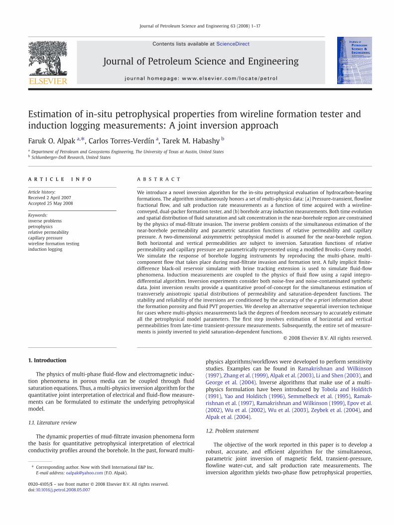
Table 2 shows the inversion results for Cases B1 and B2 along withtrue and initial-guess model parameters, and the physical boundsimposed on the search space. Inversion results indicate an accuratereconstruction of horizontal and vertical permeabilities. Parametersthat describe relative permeability and capillary pressure curves forCase B2 are also accurately resolved. True, initial-guess, and invertedsaturation functions of relative permeability (both in linear and logscales) and capillary pressure are shown in Figs. 9 through 11 for CaseB2. Pre- and post-inversion WFT data fits are shown in Fig. 12(a)through (c) for transient-pressure, in Fig. 12(d) for flowline water-cut,and in Fig. 12(e) for salt production rate. The panels of Fig. 13 showpre- and post-inversion fits of the IL data for one of the receiverlocations and for three tool frequencies.

Interestingly, the accuracy of the reconstruction of horizontalpermeability and oleic-phase end-point relative permeability ismarginal for Case B1. We attribute this behavior to the (limited)sensitivity of the inversion with respect to the adaptively computedregularization parameter, ξ. The selection of the regularizationparameter is linked to the condition number of the (Gauss–Newton)Hessian matrix. Over the course of nonlinear iterations, when thecondition number decreases below a pre-specified threshold, theregularization parameter is calculated as a small fraction of the largesteigenvalue of the Hessianmatrix. Inversion results for Cases B1 and B2exhibit limited sensitivity to the choice of this condition number andto the choice of a (small) regularization fraction. For Cases B1 and B2,the inverse problem solution appears to lie in the neighborhood of arelatively flat cost function. Overall, multi-physics measurementsprovide satisfactorily accurate reconstructions of model parameters.

5.5. Case C

Both WFT and IL measurements of Case B are contaminated with1% random Gaussian noise. Everything else is kept invariant as in CaseB2. Table 3 reports three sets of inversion results. All modelparameters are simultaneously inverted in Case C1. The comparisonof inversion results of Case C1 with respect to inversion results of CaseB2 indicates that the presence of measurement noise negativelyaffects the simultaneous inversion approach. Except for the invertedvalues of end-point saturations, results for the values of the remainingmodel parameters exhibit inaccurate reconstructions. As a remedy to

Table 2Petrophysical inversion results for the anisotropic formation model. Modified Brooks–Corey functions are used to represent two-phase relative permeability and capillary pressurecurves. Noise-free, synthetically generated measurements are input to the inversion. Results are reported for Cases A1, A2, B1, and B2, respectively

Variable Units True In.-guess and Bounds Inverted

Initial water saturation (= Irreducible water saturation) [fraction] 0.30 0.10 [0.05–0.40] 0.30 0.30 0.30 0.30Residual oil saturation [fraction] 0.20 0.10 [0.05–0.35] 0.20 0.20 0.20 0.20End-point relative permeability for aqueous phase [fraction] 0.20 0.50 [0.05–0.60] 0.12 0.13 0.19 0.21End-point relative permeability for oleic phase [fraction] 0.80 0.50 [0.20–1.00] 0.22 0.47 0.72 0.79Pore-size distribution index [dimensionless] 2.00 2.50 [1.50–3.00] N/A 1.95 N/A 2.01Capillary-entry pressure [psi] 1.00 1.50 [0.50–4.00] N/A 0.98 N/A 1.03Formation horizontal permeability [mD] 50.00 100.0 [10.0–250.0] 109.81 79.32 54.68 49.20Formation vertical permeability [mD] 10.00 50.0 [4.0–100.0] 84.27 14.75 10.66 9.61


this problem, we assume that the model parameters that govern thecapillary pressure function, namely, pore-size distribution index andcapillary-entry pressure are a priori known. The first inversion withstipulated capillary pressuremodel parameters, referred to as Case C2,involves a blind choice of criteria for the computation of theregularization parameter. The second set of inversion results (referredto as Case C3) provides reconstructions of model parameters for thecase where we optimize the regularization parameter throughexhaustive experimentation (expert-mode inversion). Inversionresults provide a quantitative proof-of-concept for the simultaneousestimation of a transversely anisotropic spatial distribution ofpermeability and saturation-dependent functions from noisy two-phase flow and IL measurements. Inversion results exhibit limitedsensitivity to the choice of regularization parameter.

As demonstrated in Cases C1, C2, and C3 a priori knowledge aboutpore-size distribution index and capillary-entry pressure are ofprimary importance. The more accurately these parameters areconstrained the better conditioned the inverse problem. Preciseknowledge of the a priorimodel for these parameters becomes crucialfor the accuracy and non-uniqueness of the model parametersinverted from noisy field measurements. In fact, overall results forCase C indicate that the quality of prior knowledge about pore-sizedistribution and capillary-entry pressure parameters ultimatelydetermines the reliability and accuracy of the inversion. Capillarypressure tests (conducted on cores of the same rock and fluid type asthe ones in the formation of interest) and accurate interpretations ofNMR measurements across the same formation may potentiallyprovide the information necessary for the construction of a reliablea priori model.

5.6. Case D

In Case D we assume a three-day long process of mud-filtrateinvasion. A realistic dual-pulse liquid production rate schedule, shownin Fig. 7(c), is used for the formation test. WFT measurements areacquired over the entire saturation range as suggested by thestabilized flowline water-cut measurements shown in Fig. 8(c). Weconsider multi-probe transient-pressure, water-cut, and magneticfield measurements to construct the data vector. We also assume thatthe measurements are contaminated with Gaussian random noise ofstandard deviation equal to 1% and 3% in Cases D1 andD2, respectively.As a simple starting point for our analysis, we assume that informationabout horizontal and vertical permeabilities can be determinedaccurately from conventional single-phase transient formation pres-sure test analysis. We only estimate parameters that describe therelative permeability and capillary pressure curves. Thus, the inversionproblem consists of estimating the parameters kr1

o , S1r, kr2o , S2r, η, andPce. Since we assume the availability of a priori information aboutpermeability, for testing the robustness of the inversion we relax thebounds applied to pore-size distribution and capillary-entry pressureparameters (Table 4). We constrain the inversion with a relativelywider set of physical bounds for these parameters. In other words, wedo not assume any a priori information (such as core and NMRmeasurements) about these parameters. Table 4 summarizes the

inversion results together with true and initial-guess values of modelparameters. At both levels of noise contamination (1% and 3%), theinversion provides an accurate reconstruction of parameters thatdescribe saturation functions of relative permeability and capillarypressure.

5.7. Case E

The inverse problem and themeasurements of Case D are the samefor Case E. However, in Case E, we do not enforce the assumption of apriori knowledge about horizontal and vertical permeabilities.We firstattempt to simultaneously invert all model parameters (Case E1).Inversion results indicate that the multi-physics data set (contami-nated with 1% random Gaussian noise) lacks the degrees of freedomnecessary to simultaneously estimate all model parameters. Thenegative impact of insufficient redundancy in the transient data(pressure transients are generated in response to a dual-pulseschedule as opposed to the multi-pulse schedule of Case B) togetherwith the absence of salt production rate measurements are apparentin the inversion results. Although the inversion converges to a misfitlevel equal to that of the noise, the inversion results are far fromaccurate. Extensive inversion exercises with various regularizationstrategies lead us to conclude that the simultaneous inversionapproach is riddled with model non-uniqueness.

Instead of resorting to NMR measurements to constrain thecapillary pressure parameters, we concentrate exclusively on theinformation content of transient formation pressure measurements.Based on single-phase inversions of transient-pressure measurementswith average fluid properties and with various regularizationweights,we determine the following ranges for horizontal and verticalpermeabilities: 55 to 60 mD and 9 to 12 mD, respectively.Subsequently, we perform the inversion of parameters that describerelative permeability and capillary pressure curves. In the latterinversions, previously inverted horizontal and vertical permeabilitiesremain fixed. We describe two examples with limiting values ofhorizontal and vertical permeability stipulated as a priori informationfor the inversion (Cases E2 and E3). Table 5 displays the post-inversionreconstructions as well as the true and initial-guess values of modelparameters input to the inversion. Table 5 also documents theparameter bounds enforced within the constrained inversion. Resultsindicate accurate reconstructions for end-point saturations and for theend-point relative permeability of the aqueous phase. Inversionresults for pore-size distribution index, capillary-entry pressureparameters, and oleic-phase end-point relative permeability exhibitlimited sensitivity to the choice of stipulated horizontal and verticalpermeabilities. Overall, the accuracy of the inverted parameters issatisfactory.

5.8. Case F

Limiting values of the ranges for horizontal and vertical perme-ability ([55–60 mD] and [9–12 mD] derived from single-phaseanalysis) are taken as initial-guess values. Everything else about thiscase remains the same as in Case E. Inversions are performed for all

Fig. 8. Dual-packer water-cut measurements for the various study cases considered inthis paper: (a) Case A; (b) Cases B, C, and G; (c) Cases D, E, and F.

Fig. 9. Reconstruction of the parametric two-phase relative permeability functions forCase B2.

Fig. 10. Reconstruction of the parametric two-phase relative permeability functions forCase B2. Relative permeability values are plotted on a logarithmic scale.

Fig. 11. Reconstruction of the parametric capillary pressure function for Case B2.


parameters. Results are shown for two cases. Case F1 uses initial-guessvalues of 55 and 9 mD for the horizontal and vertical permeability,respectively. Initial-guess values for other model parameters are thesame as in Cases E2 and E3. Multi-physics measurements arecontaminated with 1% noise. True, inverted, and initial-guess values,and bounds for all model parameters are shown in Table 6. In Case F2,initial-guess values of horizontal and vertical permeability arechanged to 60 and 12 mD, respectively. Initial-guess values for othermodel parameters remain the same as in Case F1. Multi-physicsmeasurements are contaminated with 3% noise. Table 6 also displaysthe true, inverted, and initial-guess values for all model parameters.Inversion results indicate satisfactory reconstructions of modelparameters associated with relative permeability and capillary

pressure curves under the deleterious influence of measurementnoise. A slight improvement is obtained for the values of horizontaland vertical permeability compared to previous inversions.

5.9. Case G

For the above-described inversion studies we assumed that theviscosities of the aqueous and oleic phases (denoted by μw and μo,respectively) are a priori known. In Case Gwe relax this assumption by

Fig. 12. Pre- and post-inversion data fits for transient-pressure measurements simulated for the acquisition by (a) the observation probe 1, (b) the observation probe 2, and (c) thedual-packer module. Panels (d) and (e) show pre- and post-inversion data fits for flowline water-cut and salt production rate measurements. Data fits are shown for Case B2.


introducing perturbations to the true viscosity ratio, μo/μw=0.28. Thisis accomplished by keeping the value of the aqueous-phase viscosityconstant and making perturbations to the value of the oleic-phaseviscosity. We select the measurement and inversion model chacter-istics of Case C3 as the base case. We work with measurementscontaminated with 1% random Gaussian noise. Table 7 displays thetrue, inverted, and initial-guess values, and inversion bounds for allmodel parameters. Case G1 encompasses the base case where theinversion is performed using true values of fluid viscosities, hence,using the true viscosity ratio. Inversions are also performed withperturbed viscosity ratio values of 0.39, 0.59, and 0.78. Inversionresults for these cases are reported in Cases G2, G3, and G4 of Table 7,

respectively. Consistent with our expectations, the inversion case withthe unperturbed viscosity ratio value (Case G1) yields a relativelyaccurate reconstruction of inverted model parameters. As an inter-esting outcome, the reconstruction of the values of model parametersstill remains acceptable for perturbed viscosity ratio values of 0.39(Case G2) and 0.59 (Case G3). However, the accuracy of the invertedmodel parameters significantly breaks down above a viscosity ratiovalue of 0.59.

Wewould like to point out that in the investigated perturbed caseswe assume that the model parameters that govern the capillarypressure function, namely, pore-size distribution index and capillary-entry pressure are a priori known. In addition to the described

Fig. 13. Pre- and post-inversion data fits for electromagnetic induction logging (IL) measurements. Electromagnetic data are shown only for one receiver location for 3 frequencies:∼25 kHz in panels (a) and (b), ∼50 kHz in panels (c) and (d), and ∼100 kHz in panels (e) and (f). Complex-valued primary-field data are used to perform the inversions described inthis paper. Data fits are shown for Case B2.


sensitivity study, we performed extensive inversions under theinfluence of a perturbation to the fluid viscosity ratio. Inaccurateinversion results were consistently obtained for (perturbed viscosityratio) inversions performed for cases where the capillary pressuremodel parameters are included in the simultaneous inversion togetherwith the remaining model parameters. These inversions helped usreach the following conclusion: For caseswhere knowledge of the fluidviscosities involves large uncertainty, accuracy of the inverted model

parameters is controlled by the availability of information about theparameters governing the capillary pressure function.

5.10. Cramer–Rao uncertainty bounds

We quantify the uncertainty of the estimated values of petrophy-sical parameters with the calculation of Cramer–Rao bounds using anapproximation to the Estimator's Covariance Matrix, ECM. Probable

Table 3Petrophysical inversion results for the anisotropic formation model. Modified Brooks–Corey functions are used to represent two-phase relative permeability and capillary pressurecurves. Synthetically generated measurements are contaminated with 1% random Gaussian noise. Inversion results are reported for Cases C1, C2, and C3, respectively

Variable Units True Initial-guess and Bounds Inverted

Initial water saturation (= Irreducible water saturation) [fraction] 0.30 0.10 [0.05–0.40] 0.30 0.30 0.30Residual oil saturation [fraction] 0.20 0.10 [0.05–0.35] 0.20 0.20 0.20End-point relative permeability for aqueous phase [fraction] 0.20 0.50 [0.05–0.60] 0.13 0.18 0.21End-point relative permeability for oleic phase [fraction] 0.80 0.50 [0.20–1.00] 0.51 0.68 0.83Pore-size distribution index [dimensionless] 2.00 2.50 [1.50–3.00] 2.24 N/A N/ACapillary-entry pressure [psi] 1.00 1.50 [0.50–4.00] 1.22 N/A N/AFormation horizontal permeability [mD] 50.00 100.0 [10.0–250.0] 78.19 58.21 48.00Formation vertical permeability [mD] 10.00 50.0 [4.0–100.0] 15.17 11.33 9.63

Table 4Petrophysical inversion results for the anisotropic formation model. Modified Brooks–Corey functions are used to represent two-phase relative permeability and capillary pressurecurves. Synthetically generated measurements are contaminated with 1% and 3% random Gaussian noise. Inversion results are reported for Cases D1 (1% noise) and D2 (3% noise),respectively. An italic font is used to identify values of stipulated petrophysical parameters


Initial water saturation (= Irreducible water saturation) [fraction] 0.30 0.10 [0.05–0.40] 0.30 0.30Residual oil saturation [fraction] 0.20 0.10 [0.05–0.35] 0.20 0.20End-point relative permeability for aqueous phase [fraction] 0.20 0.50 [0.05–0.60] 0.20 0.20End-point relative permeability for oleic phase [fraction] 0.80 0.50 [0.20–1.00] 0.80 0.80Pore-size distribution index [dimensionless] 2.00 4.00 [1.00–5.00] 2.02 1.98Capillary-entry pressure [psi] 1.00 2.00 [0.50–12.00] 0.99 0.97Formation horizontal permeability [mD] 50.00 50.00 [N/A] N/A N/AFormation vertical permeability [mD] 10.00 10.00 [N/A] N/A N/A


ranges are estimated through Cramer–Rao bounds for model para-meters inverted from noisy measurements. The ECM is approximatedby applying Taylor series expansion on the objective function aroundthe converged solution (estimator). The assumption for derivingbounds from an approximate ECM is that the errors in themeasurements are random and Gaussian. Alpak (2005) presents thedetails of deriving Cramer–Rao uncertainty bounds from an approx-imate ECM.

Table 8 shows Cramer–Rao uncertainty bounds for example caseswhere the measurements input to the inversion are contaminatedwith zero-mean Gaussian random noise. The performance of theCramer–Rao bounds in capturing the true solution within theuncertainty bounds is mixed. For relatively more accurately invertedparameters, e.g. residual saturations, estimated bounds remainsufficiently small indicating that the multi-physics approach success-fully constrains the stability and non-uniqueness of the inversion. Onthe other hand, for a number of other parameters the true solution liesbeyond the estimated bounds. Overall, multi-physics joint inversionreconstructs the petrophysical model reasonably well for the analyzedcases. In the past, Cramer–Rao bounds performed well for thepetrophysical inversion of IL measurements (Alpak et al., 2006).However, for the investigated multi-physics multi-datatype problem,the suitability of the Cramer–Rao technique remains inconclusive. It isknown that for strongly nonlinear inverse problems the approxima-tion of ECMmay become less accurate. We attribute the unsatisfactory

Table 5Petrophysical inversion results for the anisotropic formation model. Modified Brooks–Coreycurves. Synthetically generated measurements are contaminated with 1% random Gaussian nused to identify values of stipulated petrophysical parameters

Variable Units True

Initial water saturation (= Irreducible water saturation) [fraction] 0.3Residual oil saturation [fraction] 0.2End-point relative permeability for aqueous phase [fraction] 0.2End-point relative permeability for oleic phase [fraction] 0.8Pore-size distribution index [dimensionless] 2.0Capillary-entry pressure [psi] 1.0Formation horizontal permeability [mD] 50.0Formation vertical permeability [mD] 10.0

performance of the Cramer–Rao technique to the strong nonlinearityof the investigated multi-physics inverse problem involving two-phase flow.

6. Discussion

Within the context of numerical examples we considered the useof multi-physics inversion to design an optimal data-acquisitionschedule for the interpretation of WFTmeasurements. In order for themulti-physics inversion algorithm to yield physically consistentreconstructions the measurements must exhibit sufficient sensitivitytomodel parameters. Themethodology may fail, if the invasion is verythin, and thus, below the resolution of the inverted measurements. Amulti-pulse rate-schedule, presence of salt production rate informa-tion, and a sufficiently-long sampling-time interval are essential forthe accurate simultaneous reconstruction of all themodel parameters.For water-based mud-filtrate invasion insufficient sampling of themovable saturation front significantly compromises the ability of theinversion to estimate the oleic-phase end-point relative permeability.

Despite not explored in this paper, the multi-physics inversionapproach could also be utilized to enhance the information content ofIL measurements with respect to flow-related petrophysical proper-ties of rock formations. Specifically, the number of inductionfrequencies or receivers can be chosen to provide selective deepeningof the zone of response, and hence to improve the detection and

functions are used to represent two-phase relative permeability and capillary pressureoise. Inversion results are reported for Cases E1, E2, and E3, respectively. An italic font is

In.-guess and Bounds Inverted

0 0.10 0.10 0.10 [0.05–0.40] 0.30 0.30 0.300 0.10 0.10 0.10 [0.05–0.35] 0.20 0.19 0.200 0.50 0.50 0.50 [0.05–0.60] 0.16 0.19 0.170 0.50 0.50 0.50 [0.20–1.00] 0.65 0.70 0.670 2.50 4.00 4.00 [1.00–5.00] 1.93 2.48 2.000 1.50 2.00 2.00 [0.50–12.00] 0.91 1.45 0.980 100.00 55.00 60.00 [10.00–250.00] (E1) 61.71 N/A N/A0 50.00 9.00 12.00 [4.00–100.00] (E1) 12.41 N/A N/A

Table 6Petrophysical inversion results for the anisotropic formation model. Modified Brooks–Corey functions are used to represent two-phase relative permeability and capillary pressurcurves. Synthetically generated measurements are contaminated with 1% and 3% random Gaussian noise. Inversion results are reported for Cases F1 (1% noise) and F2 (3% noise)respectively


Initial water saturation (= Irreducible water saturation) [fraction] 0.30 0.10 0.10 [0.05–0.40] 0.30 0.30Residual oil saturation [fraction] 0.20 0.10 0.10 [0.05–0.35] 0.19 0.20End-point relative permeability for aqueous phase [fraction] 0.20 0.50 0.50 [0.05–0.60] 0.21 0.17End-point relative permeability for oleic phase [fraction] 0.80 0.50 0.50 [0.20–1.00] 0.85 0.69Pore-size distribution index [dimensionless] 2.00 4.00 4.00 [1.00–5.00] 2.68 2.05Capillary-entry pressure [psi] 1.00 2.00 2.00 [0.50–12.0] 1.54 1.06Formation horizontal permeability [mD] 50.00 55.0 60.0 [45.0–70.0] 46.57 58.02Formation vertical permeability [mD] 10.00 9.00 12.0 [5.00–15.0] 8.86 11.48

Table 7Petrophysical inversion results for the anisotropic formation model. Modified Brooks–Corey functions are used to represent two-phase relative permeability and capillary pressurecurves. Synthetically generated measurements are contaminated with 1% random Gaussian noise. Inversion results are reported for Cases G1 (μo/μw=0.28), G2 (μo/μw=0.39), G3 (μo/μw=0.59), and G4 (μo/μw=0.78), respectively


Initial water saturation (= Irreducible water saturation) [fraction] 0.30 0.10 [0.05–0.40] 0.30 0.30 0.30 0.30Residual oil saturation [fraction] 0.20 0.10 [0.05–0.35] 0.20 0.20 0.19 0.20End-point relative permeability for aqueous phase [fraction] 0.20 0.50 [0.05–0.60] 0.21 0.18 0.26 0.08End-point relative permeability for oleic phase [fraction] 0.80 0.50 [0.20–1.00] 0.83 0.99 0.97 0.84Pore-size distribution index [dimensionless] 2.00 N/A N/A N/A N/A N/ACapillary-entry pressure [psi] 1.00 N/A N/A N/A N/A N/AFormation horizontal permeability [mD] 50.00 100.0 [10.0–250.0] 48.00 56.76 44.39 109.80Formation vertical permeability [mD] 10.00 10.0 [4.0–100.0] 9.63 11.51 4.62 25.24


assessment of the spatial distribution of phase saturations. Redun-dancy of electromagnetic data may further contribute to the accuratereconstruction of petrophysical model parameters.

In most of the investigated cases, the WRGN minimizationalgorithm converged to an improved solution without the use ofSPSA-based helper methods (see, Appendix A). SPSA-based helpermethods enhance the WRGN inversion results considerably in CasesD2 and F2 where the level of random Gaussian noise contaminationwas 3%.

7. Summary and conclusions

We formulated and implemented a robust and accurate hybridoptimization algorithm for the simultaneous inversion of anisotropicformation permeabilities and parametric forms of relative perme-ability and capillary pressure curves. The hybrid inversion algorithmallows a two-way coupling between a (global) simultaneous pertur-bation stochastic approximation (SPSA) technique, and a (local)weighted and regularized Gauss–Newton (WRGN) technique.

The proof-of-concept inversion exercises considered in this paperconsistently show the benefit of the multi-physics approach for thequantitative integration of several types of measurements into a two-phase fluid model of petrophysical variables. Use of multi-physicsmeasurements within the hybrid optimization framework reducesnon-uniqueness of the inversion. Thus, the joint inversion algorithmefficiently and stably estimates the anisotropic permeabilities andsaturation functions of relative permeability and capillary pressure.

Table 8Cramer–Rao uncertainty bounds for example cases where measurements are contaminated with zero-mean Gaussian random noise

Variable Case C1 Case C2 Case C3 Case D1 Case D2 Case F1 Case F2

Irreducible water saturation [fraction] 3.74e−05 4.34e−05 3.71e−05 6.04e−05 1.82e−04 6.48e−05 1.84e−04Residual oil saturation [fraction] 2.99e−04 6.05e−04 2.32e−04 3.16e−04 9.18e−04 3.21e−04 9.91e−04End-point relative permeability for aqueous phase [fraction] 3.65e−03 1.98e−02 6.07e−03 2.67e−04 8.09e−04 2.06e−03 1.27e−02End-point relative permeability for oleic phase [fraction] 1.31e−02 6.75e−02 2.21e−02 6.61e−04 2.04e−03 7.82e−03 4.41e−02Pore-size distribution index [dimensionless] 2.20e−02 N/A N/A 1.89e−02 4.63e−02 1.19e−02 4.63e−0Capillary-entry pressure [psi] 2.25e−02 N/A N/A 1.28e−02 3.33e−02 1.46e−02 3.48e−0Formation horizontal permeability [mD] 1.02 1.09 1.03 N/A N/A 1.01 1.07Formation vertical permeability [mD] 1.03 1.08 1.03 N/A N/A 1.01 1.06

e,

However, the accuracy of the simultaneous inversion approach issubject to the availability of a priori information about parametersthat govern the capillary pressure function. Accurate reconstructionsof anisotropic permeabilities, and parametric relative permeabilityand capillary pressure curves are obtained from synthetic multi-physics measurements contaminated with random Gaussian noise.For cases where knowledge of the fluid viscosities involves largeuncertainty, accuracy of the invertedmodel parameters is constrainedby information about the governing parameters of the capillarypressure saturation function.

A sequential inversion workflow is developed to solve estimationproblems where formation tester (WFT) and induction logging (IL)measurements lack the necessary degrees of freedom to simulta-neously estimate the entire set of petrophysical model parameters. Asingle-phase pre-processing of late-time multi-probe transient for-mation pressuremeasurements provides a closer starting point for themulti-physics inversion of horizontal and vertical permeabilities. Thisapproach is efficient and accurate with conventional rate pulseschedules and in the presence of noisy measurements.

Robustness of the multi-physics inversion with respect to end-point saturations can only be achieved with array inductionmeasurements. This conclusion emerges as the result of extensiveinversion exercises performed with various combinations of measure-ment types.

Currently, the only undesirable feature of the developed simulta-neous multi-physics inversion approach is the requirement of expert-mode input when all of the model parameters are estimated in the

22


presence of noisy measurements. Careful adjustment of measurementand regularization weights is necessary to obtain accurate inversionresults.

The parametric formulation of the multi-physics inversion pro-blem allows one to use a relatively small number of model parameters.When the initial-guess model is sufficiently close to the (global)minimum, aweighted and regularized Gauss-Newton search direction(used by the WRGN technique) provides rapid convergence. For theinvestigated problems, WRGN-based inversions required a maximumof 15 to 20 Gauss–Newton iterations to achieve convergence.However, the computation time required by the inversions increased3 to 5 fold when a SPSA-based helper algorithmwas activated togetherwith the WRGN approach.

Acknowledgements

This work was funded by UT Austin's Center of Excellence inFormation Evaluation, jointly sponsored by Baker Atlas, Halliburton,Schlumberger, Anadarko Petroleum Corporation, Shell InternationalE&P, ConocoPhillips, ExxonMobil, TOTAL, and the Instituto MexicanoDel Petróleo. We are also grateful to Dr. Vladimir Druskin for providingus with the integro-differential computer code KARID to simulateinduction logging measurements.

Appendix A. Hybrid optimization algorithm

The inversion algorithm makes us of a local minimizer based onthe weighted least-squares technique and two global minimizersbased on the stochastic approximation (SA) technique. Technicaldetails concerning these two techniques are given below.

A.1. Weighted least-squares inversion

For inversion we minimize Eq. (11) using a weighted least-squaresalgorithmwith a regularized Gauss-Newton search direction (WRGN).Let us first construct a local quadratic model of the objective function.The quadratic model is formed by taking the first three terms of theTaylor series expansion of the objective function around the currentkth iteration (xk), as follows:

C xk þ pkð Þ≈C xkð Þ þ gT xkð Þ � pk þ12pTk � G xkð Þ � pk; ðA� 1Þ

where the superscript T indicates transposition and pk=xk +1−xk is thestep in xk toward the minimum of the objective function, C(x). Thevector g(x)=∇C(x) is the gradient vector of the objective function andis given by the following expression:

g xð Þ ¼ ξ JT xð Þ �WTd �Wd � e xð Þ þWT

x �Wx � x−xp�

: ðA� 2Þ

In Eq. (A-2), J(x) is the M×N Jacobian matrix, and is given by

J xð Þ ¼ Jmn≡∂em∂xn

; m ¼ 1;2;3;…;M; n ¼ 1;2;3;…;N�;"ðA� 3Þ

In the regularized Gauss–Newton search method, one discards thesecond-order derivatives within the Hessian matrix, G, to avoidexpensive computations. Then, the Hessian matrix reduces to

G xð Þ ¼ WTx �Wx þ ξ JT xð Þ �WT

d �Wd � J xð Þ; ðA� 4Þ

which is a positive semi-definitematrix. If λj and vj are the eigenvaluesand the corresponding orthonormal eigenvectors of the N×N realsymmetric matrix G

G � vj ¼ λjvj; ðA� 5Þsuch that

vTi � vj ¼ δij: ðA� 6Þ

Then,

λj ¼vTj � G � v

j

kvjk2¼ kWx � vjk2 þ ξkWd � J � vjk2≥0; ðA� 7Þ

Hence, G is a positive semi-definite matrix. The Hessian matrix G canbe constructed to be a positive-definite matrix by enforcing a propervalue of ξ. The minimum of the right-hand side of Eq. (A-1) is achievedif pk is a minimum of the quadratic function

/ pð Þ ¼ gT xkð Þ � pþ 12pT � G xkð Þ � p: ðA� 8Þ

The function ϕ(p) has a stationary point (a minimum, a maximum or asaddle point) at po, if the gradient vector of ϕ(p) vanishes at po, i.e.,

j/ poð Þ ¼ G � po þ g ¼ 0: ðA� 9Þ

Thus, the stationary point is the solution to the following set of linearequations:

G � po ¼ −g ðA� 10Þ

with the Hessian approximated by Eq. (A-4) is called the regularizedGauss–Newton search direction. The regularized Gauss–Newtonminimization approach has a rate of convergence that is slightlyslower than quadratic but significantly faster than linear. It providesquadratic convergence in the neighborhood of the minimum (Nocedaland Wright, 1999). A significant advantage of the WRGN method overalternative gradient-basedminimization techniques such as conjugategradient, quasi-Newton, and steepest descent, is its nearly-quadraticrate of convergence. This enhancement in the rate of convergence ispossible because of the use of the Jacobian matrix (Nocedal andWright, 1999). For the parametric inversion problem considered inthis paper, the number of unknown model parameters is rathermoderate. Therefore, the evaluation of the entries of the Jacobianmatrix can be performed by finite differences without incurring onexcessive computational costs.

A.2. Further enhancements on WRGN

The invertedmodel parameters, x, are constrained to bewithin theirphysical bounds using a nonlinear transformation (Alpak, 2005). Such anonlinear transformation maps a constrained minimization probleminto an unconstrained one. A backtracking line search algorithm is usedalong the descent direction to guarantee a reduction of the objectivefunction from one iteration to the next. The choice of the Lagrangemultiplier, ξ, is adaptively linked to the condition number of theHessianmatrix of the WRGN method. The weight of the misfit term in theobjective function is progressively increased with respect to theregularization term as the inversion algorithm iterates toward theminimum value of the objective function. Evaluation of the Hessianmatrix is the most computationally intensive part of the inversion. Fouralternative approximate update methods for the Hessian matrix, whicheliminate expensive computations, are employed to accelerate theinversions. The explored approximation schemes include the following:Broyden symmetric rank-one, Powell–Symmetric–Broyden (PSB) rank-two, Davidson–Fletcher–Powell (DFP) rank-two, andBroyden–Fletcher–Goldfarb–Shanno (BFGS) rank-two update methods (Gill et al., 1981).

A.3. Hybridization of WRGN with helper methods

The quadratic approximation of the objective function, C(x),shown in Eq. (A-1), lives in the space of model parameters sufficientlyclose to the minimum. As such, the WRGN direction is rendered adescent direction. When applied properly, regularization certainlyhelps to further increase the spectral radius of this model space bysharpening the objective function in the vicinity of minimum.


However, for cases where a priori information is significantly deficient,initial-guess locations may be located far away from the spacedescribed by the spectral radius of a WRGN step. Hence, an algorithmthat relies solely on the WRGN approach may be trapped in a localminimum. A helper routine that implements a global optimizationapproach can be used to perform theminimization in the region of themodel spacewhere the quadratic approximation (with regularization)can locate the minimum accurately.

A great majority of global optimization techniques are plagued bythe requirement of intensive forward modeling. Therefore, ourinversion algorithm may be rendered prohibitively slow since wemake use of robust and accurate forward solvers instead of proxymethods (i.e., artificial neural networks, etc.). The accuracy of suchproxy techniques depend principally on the extent of initial simula-tion investment. For the purpose of maintaining the generality of theinverse solver, we avoid the use of proxy modeling approach. Tomitigate a potential initial-guess related local-trapping problem,among the investigated global optimization techniques, simultaneousperturbation stochastic approximation (SPSA) technique introducedby Spall (1992) provided an optimal balance between accuracy andcomputational efficiency for our inversion algorithm. In our imple-mentation, the user can activate an option such that the optimizationwill start with a global approach. Upon satisfaction of globalconvergence criteria, the inversion algorithm may switch to a WRGNtechnique until the WRGN convergence criteria are satisfied. If theWRGN technique fails to satisfy the convergence criteria, a globalhelper routine is automatically reactivated. If convergence is still notachieved after a given number of global–local interactions, inversionwill restart itself by drawing a new initial-guess location using arandom number generator. The selection of the new initial-guesslocation is constrained by the physical constraints already imposed onthe SPSA andWRGNmethods. The above-described two-way couplingbetween SPSA and WRGN techniques is graphically demonstrated inFig. 2. This figure is generated for the hybridization of WRGN withASPSA that will be described in a further section of the paper.Alternatively, depending upon the choice made by the user, SPSA orWRGN methods can also be run independently. Our hybrid optimizerdeveloped in FORTRAN90 drives ECLIPSE and KARID, which, in turn,together act as an objective function evaluator. A UNIX interfaceestablishes communication between the optimization routines andthe multi-physics simulation.

Two variants of SPSA are implemented. The first helper algorithmis a standard implementation of SPSA with simple enhancements forimposing bounds and search direction efficiency, referred to asSSPSA. A second helper routine implementation makes use of astochastic gradient averaging approach within SPSA for determiningsmooth search directions to mitigate possible large jumps in modelspace. This helper approach is here referred to as ASPSA. Ourimplementations of SPSA follow detailed guidelines provided bySpall (1998).

A.3.1. SSPSA techniqueLet us minimize a differentiable, modified objective function

F xð Þ ¼ kWd � e xð Þk2−χ2n o

; ðA� 11Þ

where F:RN→R1. At the minimum, the modified objective functionsatisfies

jF xkð Þ ¼ g xkð Þ ¼ 0: ðA� 12Þ

A great majority of SA algorithms based on finite-difference methodsrequire 2N evaluations of F at each iteration. However, the SPSAtechnique only requires 2Q (Q≥1) evaluations of F at each iteration,where for large N one typically has Q≪N. Therefore, SPSA mayprovide significant algorithmic efficiency as long as the number of

iterations does not increase to counterbalance the reduced amount ofmodified objective function evaluations per iteration.

Let xk denote the estimate for x at the kth iteration, the stochasticapproximation algorithm has the following standard form

xkþ1 ¼ xk−akgk xkð Þ; ðA� 13Þwhere ak is the so-called “gain sequence” that satisfies the conditionslisted by Spall (1992). The simultaneous perturbation estimate for gk(xk)is determined as follows:

Let δkaRN be a vector of N mutually independent zero-meanrandom variables, δk=[δk1,…, δkN]T, satisfying the conditions given bySpall (1992). The principal condition for the convergence of SPSA isthat E{||δk−1||}, or some higher inverse moment of δk be bounded. Thiscondition distinctly precludes δk from being uniformly or normallydistributed. Let {δk} be a mutually independent sequence with δkindependent of xo, x1,…, xk. Theoretically, no additional assumption isnecessary for the specific distribution for δk. For the numericalimplementation we assume that δk is symmetrically Bernoullidistributed. Also, let ck be a positive scalar, and

Y þð Þ ¼ F xk þ ckδkð Þ ðA� 14Þ

and

Y −ð Þ ¼ F xk−ckδkð Þ: ðA� 15ÞThen, the estimate of gk(xk) is given by

gk xkð Þ ¼ Y þð Þ−Y −ð Þ

2ckδk1…

Y þð Þ−Y −ð Þ

2ckδkN

� �TðA� 16Þ

This estimate differs from the usual stochastic finite-differenceapproximation in that only two evaluations (instead of 2N) are used.The name “simultaneous perturbation” as applied to Eq. (A-16) arisesfrom the fact that all elements of thexk vector are varied simultaneously.

A.3.2. ASPSA techniqueAside from evaluating Eq. (A-13) with gk(xk) as in Eq. (A-16), in

ASPSA we consider using Eq. (A-13) with several independentsimultaneous perturbation approximations averaged at each iteration.Thus gk(xk) in Eq. (A-16) is replaced by

gk xkð Þ ¼ Q−1 ∑Q

j¼1g jð Þk xkð Þ; ðA� 17Þ

where each gk(j)(xk) is generated as in Eq. (A-16) based on a new pair ofevaluations that are conditionally independent of the other measure-ment pairs. Spall24 demonstrates that averaging can enhance theperformance of the SA algorithm.

References

Alpak, F.O., 2005. Algorithms for Numerical Modeling and Inversion of Multi-PhaseFluid-Flow and Electromagnetic Measurements. Ph.D. dissertation, The Universityof Texas at Austin, Austin, TX.

Alpak, F.O., Dussan V., E.B., Habashy, T.M., Torres-Verdín, C., 2003. Numerical simulationof mud-filtrate invasion and sensitivity analysis of array induction tools.Petrophysics 44, 396.

Alpak, F.O., Habashy, T.M., Torres-Verdín, C., Dussan V., E.B., 2004. Joint inversion of transient-pressure and time-lapse electromagnetic measurements. Petrophysics 45, 138.

Alpak, F.O., Torres-Verdín, C., Habashy, T.M., 2006. Petrophysical inversion of boreholearray induction logs: part I — numerical examples. Geophysics 71, F101.

Altunbay, M., Georgi, D., Zhang, G.Q., 1998. Pseudo capillary pressure from NMR data.Proceedings of the International Petroleum Congress of Turkey, October 12–14,1998.

Altunbay, M., Martain, R., Robinson, M., 2001. Capillary pressure data from NMR logsand its implications on field economics. Paper SPE 71703, in 2001 SPE AnnualTechnical Conference Proceedings, Society of Petroleum Engineers.

Archie, G.E., 1942. The electrical resistivity log as an aid in determining some reservoircharacteristics. Pet. Trans. AIME 146, 54.

Ayan, C., Hafez, H., Hurst, H., Kuchuk, F.J., O'Callaghan, A., Peffer, J., Pop, J., Zeybek, M.,2001. Characterizing permeability with formation testers. Oilfield Rev. 1 Autumnissue.


Aziz, K., Settari, A., 1979. Petroleum Reservoir Simulation. Applied Science PublishersLtd., London.

Druskin, V.L., Tamarchenko, T.V., 1988. Fast variant of partial domain method forsolution of the problem of induction logging. Geol. Geofiz. 29, 129 (in Russian,translated to English).

Epov, M., Yeltsov, I., Kashevarov, A., Sobolev, A., Ulyanov, V., 2002. Time evolution of thenear borehole zone in sandstone reservoir through the time-lapse data of high-frequency electromagnetic logging. Paper ZZ, in 43rd Annual Logging SymposiumTransactions, Society of Professional Well Log Analysts, ZZ1.

GeoQuest, Schlumberger, 2000. ECLIPSE Reference Manual 2000A.George, B.K., Torres-Verdín, C., Delshad, M., Sigal, R., Zouioueche, F., Anderson, B., 2004.

Assessment of in-situ hydrocarbon saturation in the presence of deep invasion andhighly saline connate water. Petrophysics 45, 141.

Gill, P.E., Murray, W., Wright, M.H., 1981. Practical Optimization. Academic Press,London.

Honarpour, M., Koederitz, L.F., Harvey, A.H., 1986. Relative Permeability of PetroleumReservoirs. CRC Press Inc., Boca Raton, FL.

Hunka, J.F., Barber, T.D., Rosthal, R.A., Minerbo, G.N., Head, E.A., Howard, A.Q., Hazen, G.A., Chandler, R.N., 1990. A new resistivity measurement system for deep formationimaging and high-resolution formation evaluation. Paper SPE 20559, in 1990 SPEAnnual Technical Conference Proceedings, Society of Petroleum Engineers, p. 295.

Lake, L.W., 1989. Enhanced Oil Recovery. Prentice Hall, Englewood Cliffs, NJ.Li, S., Shen, L.C., 2003. Dynamic invasion profiles and time-lapse electrical logs. Paper E

in 44th Annual Logging Symposium Transactions, Society of Professional Well LogAnalysts, E1.

Nocedal, J., Wright, S.J., 1999. Numerical Optimization. Springer-Verlag, NY.Pop, J., Badry, R., Morris, C., Wilkinson, D., Tottrup, P., Jonas, J., 1993. Vertical interference

testing with a wireline-conveyed straddle-packer tool. Paper SPE 26481, in 1993 SPEAnnual Technical Conference Proceedings, Society of Petroleum Engineers, p. 665.

Ramakrishnan, T.S., Wilkinson, D.J., 1997. Formation producibility and fractional flowcurves from radial resistivity variation caused by drilling fluid invasion. Phys. Fluids9, 833.

Ramakrishnan, T.S., Wilkinson, D.J., 1999. Water-cut and fractional flow logs from array-induction measurements. SPE Reserv. Eval. Eng. 2, 85.

Ramakrishnan, T.S., Al-Khalifa, J., Al-Waheed, H.H., Cao-Minh, C., 1997. Producibilityestimation from array-induction logs and comparison with measurements-a case

study. Paper X, in 38th Annual Logging Symposium Transactions, Society ofProfessional Well Log Analysts, X1.

Semmelbeck, M.E., Dewan, J.T., Holditch, S.A., 1995. Invasion-based method forestimating permeability from logs. Paper SPE 30581, in 1995 Annual TechnicalConference Proceedings, Society of Petroleum Engineers, p. 517.

Spall, J.C., 1992. Multivariate stochastic approximation using a simultaneous perturba-tion gradient approximation. IEEE Trans. Automat. Contr. 37, 332.

Spall, J.C., 1998. Implementation of the simultaneous perturbation algorithm forstochastic optimization. IEEE Trans. Aerosp. Electron. Syst. 34, 817.

Tobola, D.P., Holditch, S.A., 1991. Determination of reservoir permeability from repeatedinduction logging. SPE Form. Eval. 20 March issue.

Volokitin, Y., Looyestijn, W.J., Slijkerman, W.F.J., Hofman, J.P., 1999. A practical approachto obtain 1st drainage capillary pressure curves from NMR core and log data. PaperSCA-9924, presented at the International Symposium of the Society of CoreAnalysts, Golden, CO, August 1–4.

Yao, C.Y., Holditch, S.A., 1996. Reservoir permeability estimation from time-lapse logdata. SPE Form. Eval. 69 June issue.

Wu, J., 2004. Numerical Simulation of Multi-Phase Mud-Filtrate Invasion and Inversionof Formation Tester Data. Ph.D. dissertation, The University of Texas at Austin,Austin, TX.

Wu, J., Torres-Verdín, C., Proett, M.A., Sepehrnoori, K., Belanger, D., 2002. Inversion ofmulti-phase petrophysical properties using pumpout sampling data acquired witha wireline formation tester. Paper SPE 77345, in 2002 SPE Annual TechnicalConference Proceedings, Society of Petroleum Engineers.

Wu, J., Torres-Verdín, C., Sepehrnoori, K., Proett, M.A., van Dalen, S.C., 2003. A newinversion technique determines in-situ relative permeabilities and capillarypressure parameters from pumpout wireline formation tester data. Paper GG, in44th Annual Logging Symposium Transactions, Society of Professional Well LogAnalysts, GG1.

Zeybek, M., Ramakrishnan, T.S., Al-Otaibi, S.S., Salamy, S.P., Kuchuk, F.J., 2004. Estimatingmultiphase-flow properties from dual-packer formation tester interval tests andopenhole array resistivity measurements. SPE Reserv. Evalu. Eng. 40.

Zhang, J.-H., Hu, Q., Liu, Z.-H., 1999. Estimation of true formation resistivity and watersaturation with a time-lapse induction logging method. Log Anal. 40, 138.

estimation of in-situ petrophysical properties from ... · relative permeability capillary pressure...

Documents