estimation of crossing conflict at signalized intersection · pdf fileestimation of crossing...
TRANSCRIPT

Estimation of Crossing Conflict at Signalized Intersection Using High-Resolution Traffic DataGary A. Davis, Principal InvestigatorDepartment of Civil, Environmental, and Geo- Engineering University of Minnesota
March 2017
Research ProjectFinal Report 2017-08
• mndot.gov/research

To request this document in an alternative format, such as braille or large print, call 651-366-4718 or 1-800-657-3774 (Greater Minnesota) or email your request to [email protected]. Pleaserequest at least one week in advance.

Technical Report Documentation Page 1. Report No. 2. 3. Recipients Accession No.MN/RC 2017-08
4. Title and Subtitle 5. Report DateMarch 2017Estimation of Crossing Conflict at Signalized Intersection Using
High-Resolution Traffic Data 6.
7. Author(s) 8. Performing Organization Report No.Henry X. Liu, Gary A. Davis, Shengyin Shen, Xuan Di, and IndrajitChatterjee
9. Performing Organization Name and Address 10. Project/Task/Work Unit No.Department of Civil, Environmental, and Geo- EngineeringUniversity of Minnesota500 Pillsbury Drive SEMinneapolis, MN 55455
CTS #201501311. Contract (C) or Grant (G) No.(c) 99008 (wo) 155
12. Sponsoring Organization Name and Address 13. Type of Report and Period CoveredMinnesota Department of TransportationResearch Services & Library395 John Ireland Boulevard, MS 330St. Paul, Minnesota 55155-1899
Final Report14. Sponsoring Agency Code
15. Supplementary Noteshttp:// mndot.gov/research/reports/2017/201708.pdf16. Abstract (Limit: 250 words)
This project explores the possibility of using high-resolution traffic signal data to evaluate intersection safety.Traditional methods using historical crash data collected from infrequently and randomly occurring vehicle collisions can require several years to identify potentially risky situations. By contrast, the proposed method estimates potential traffic conflicts using high-resolution traffic signal data collected from the SMART-Signal system. The potential conflicts estimated in this research include both red-light running events, when stop-bar detectors are available, and crossing (i.e. right-angle) conflicts. Preliminary testing based on limited data showed that estimated conflict frequencies were better than AADT for predicting frequencies of angle crashes. With additional validation this could provide a low-cost and easy-to-use tool for traffic engineers to evaluate traffic safety performance at signalized intersections.
17. Document Analysis/Descriptors 18. Availability StatementRed light running, Signalized intersections, Traffic safety, Trafficconflicts, Right angle crashes, Traffic data
No restrictions. Document available from:National Technical Information Services,Alexandria, Virginia 22312
19. Security Class (this report) 20. Security Class (this page) 21. No. of Pages 22. PriceUnclassified Unclassified 56
Estimation of Crossing Conflict at Signalized Intersection Using High-
Resolution Traffic Data
FINAL REPORT
Prepared by:
Henry X. Liu1 Gary A. Davis2 Shengyin Shen1
Xuan Di1 Indrajit Chatterjee2
1. Department of Civil and Environmental Engineering, University of Michigan
2. Department of Civil, Environmental, and Geo- Engineering, University of Minnesota
March 2017
Published by:
Minnesota Department of Transportation
Research Services & Library
395 John Ireland Boulevard, MS 330
St. Paul, Minnesota 55155-1899
This report represents the results of research conducted by the authors and does not necessarily represent the views or policies
of the Minnesota Department of Transportation or the University of Minnesota. This report does not contain a standard or
specified technique.
The authors, the Minnesota Department of Transportation, and the University of Minnesota do not endorse products or
manufacturers. Trade or manufacturers’ names appear herein solely because they are considered essential to this report
because they are considered essential to this report.

ACKNOWLEDGMENTS
This work was supported by the MnDOT. The authors would like to thank Steve Misgen from MnDOT for
his assistance in the field deployment of the SMART-Signal system. Jingru Gao assisted with preparation
of the final report.

TABLE OF CONTENTS
CHAPTER 1: INTRODUCTION ...............................................................................................................1
1.1 Research Objectives............................................................................................................................ 1
1.2 Background and Relevant Work ......................................................................................................... 1
1.2.1 RLR Behavior Modeling ............................................................................................................... 1
1.2.2 Crossing Conflicts ........................................................................................................................ 2
1.2.3 Data Collection Methods ............................................................................................................. 2
1.3 Organization of This Report ................................................................................................................ 6
CHAPTER 2: IDENTIFYING FIRST-TO-STOP (FSTP), YELLOW-LIGHT RUNNING (YLR), AND RED-LIGHT-
RUNNING (RLR) EVENTS USING STOP BAR AND ENTRANCE DETECTORS ...............................................7
2.1 Methodology ...................................................................................................................................... 8
2.2 RLR events ........................................................................................................................................ 11
2.3 Modeling Stop-or-Go Behavior Using Advance Detector Data ........................................................ 15
2.3.1 Matching Events to Advance Detectors and Data Extraction ................................................... 15
2.3.2 Training a Stop-Or-Go Model .................................................................................................... 19
2.3.3 Predicting Stop-or-Go Behavior ................................................................................................ 21
CHAPTER 3: IDENTIFYING CROSSING CONFLICT ADVANCE DETECTORS ............................................... 24
3.1 Methodology .................................................................................................................................... 24
3.2 Stop-or-Go Behavior Prediction ....................................................................................................... 25
3.3 Crossing Conflicts Identification within Conflict Zones .................................................................... 26
3.4 Example Illustration .......................................................................................................................... 28
3.5 Crossing conflicts summary .............................................................................................................. 31
CHAPTER 4: RIGHT-ANGLE CRASH MODEL REGRESSION .................................................................... 33
4.1 Data Preparation .............................................................................................................................. 33
4.2 Statistical Analyses ........................................................................................................................... 34
CHAPTER 5: CONCLUSION ................................................................................................................. 37

REFERENCES .................................................................................................................................... 38
APPENDIX A: Data Used in Crash Prediction Analyses

LIST OF TABLES
Table 1. 1 Data collection methods comparison .......................................................................................... 3
Table 2.1 Average speed in each lane ......................................................................................................... 12
Table 2. 2 Direct information extracted from the advance detector ......................................................... 16
Table 2. 3 Description of datasets at Rhode Island/TH55 intersection ...................................................... 19
Table 2. 4 Coefficients of logistic regression............................................................................................... 19
Table 2. 5 Coefficients of logistic regression for the reduced model ......................................................... 21
Table 2. 6 Confusion matrix for prediction result ....................................................................................... 23
Table 3. 1 SMART signal data ...................................................................................................................... 26
Table 3. 2 Advance detector event record in the database ........................................................................ 29
Table 3. 3 Signal phase event record in the database ................................................................................ 29
Table 3. 4 Coefficients of the stop-or-go model ......................................................................................... 29
Table 3. 5 Stop-bar detector event record in the database........................................................................ 31
Table 3. 6 Estimated crossing conflicts ....................................................................................................... 31
Table 4. 1 Intersections with SMART-SIGNAL Data .................................................................................... 33
Table 4. 2 Results from Fitting Model with Major and Minor AADT as Angle-Crash Predictors ................ 35
Table 4. 3 Results from Fitting a Model with Minor AADT and Red-Light Running Frequency as Angle
Crash Predictors .......................................................................................................................................... 36
LIST OF FIGURES
Figure 2.1 FSTP, YLR, and RLR events classification ...................................................................................... 8
Figure 2. 2 Algorithm of RLR, YLR and FSTP identification ............................................................................ 9
Figure 2. 3 SMART-SIGNAL data visualization in time-space diagram .......................................................... 9
Figure 2.4 Intersection Boone/TH 55 layout ............................................................................................... 11
Figure 2. 5 Number of RLR vs. Traffic Volume (veh/month) ....................................................................... 12
Figure 2. 6 Number of RLR vs. traffic volume over the time of day for (a) westbound and (b) eastbound13
Figure 2. 7 Number of RLR vs. daily traffic volume in each month for (a) westbound and (b) eastbound 14
Figure 2. 8 Three scenarios when a vehicle arrives at the advance detector ............................................. 17
Figure 2. 9 Intersection Rhode Island/TH 55 layout ................................................................................... 18
Figure 2. 10 ROC (Receiver Operating Characteristic) curve in R ............................................................... 23
Figure 3. 1 Flowchart of identifying crossing conflict ................................................................................. 25
Figure 3. 2 Splitting conflict zones .............................................................................................................. 27
Figure 3. 3 Illustration of the identified crossing conflict ........................................................................... 28
Figure 3. 4 ROC (Receiver Operating Characteristic) curve in R ................................................................. 30

EXECUTIVE SUMMARY
Intersection safety has always been a critical concern to traffic engineers. Right-angle crashes are
particularly important in intersection safety since they often involve severe crashes at signalized
intersections. Traditionally, the number of crashes is a direct measure of intersection safety. However,
crashes are rare events and it can take one or more years to collect sufficient data for safety assessment.
Therefore, traditional methods, either using historical crash data collected from infrequent and random
vehicle collisions or potential traffic conflicts estimated from microscopic traffic simulators, which
generally assume accident-free conditions, cannot provide evaluations of intersection safety that are both
accurate and timely.
This project explores the possibility of using high-resolution traffic signal data, which can be directly
collected from existing loop detector systems, to evaluate intersection safety. In this project, we
developed a method to estimate potential traffic conflicts using high-resolution traffic signal data
collected from the SMART-Signal system, which has been deployed at over 100 intersections in the Twin
Cities. The potential conflicts estimated in this research include both red-light running events, when stop-
bar detectors are available, and crossing (i.e., right-angle) conflicts. With the estimated conflicts, a
regression model was developed to determine if adding a measure of crossing conflict to a more standard
model containing annual average daily traffic (AADTs) could improve the ability to predict angle crashes
at signalized intersections. Limited testing showed that estimated conflict frequencies were better than
AADT for predicting frequencies of angle crashes. With additional validation this could provide a low-cost
and easy-to-use tool for traffic engineers to evaluate traffic safety performance at signalized intersections.
1
CHAPTER 1: INTRODUCTION
About one million collisions occur at signalized intersections in the U.S. each year (Retting et al., 1998).
Thus, intersection safety becomes a critical concern to traffic engineers.
Right angle crashes are very important in the intersection safety, because they are more likely to involve
severe crashes at signalized intersections. Based on the data in a study conducted in the state of Florida
(Abdel-Aty et al., 2005), it was found that around 45% of right-angle crashes involve injury whereas only
around 25% of other crashes involve injury. The number of crashes is a direct measure of intersection
safety. However, they are fortunately rare events and it thus takes a long time to collect sufficient data
for safety assessment. For example, Mitra et al. (2002) studied the frequency of right angle crash using 52
four-legged signalized intersections in Singapore over 8 years (1992-1999). Poch and Mannering (1996) fit
an angle crash frequency model for 63 four-legged intersections over 7 years (1987-1993).
Since the traditional method of evaluating the intersection safety relies heavily upon crash data,
researchers have proposed surrogate methods to assess intersection safety as an alternative to crash
data. Perkins and Harris (1967, 1968) first proposed the concept of traffic conflict and it was defined by
Amundson and Hyden (1977) as “an observed situation in which two or more road users approach each
other in space and time to such an extent that there is a risk of collision if their movement remains
unchanged.” Conflicts occur much more frequently than actual collisions, and therefore have significantly
greater sample sizes than do crash counts. This can make it easier and less costly to analyze safety-related
characteristics of roadway segments and intersections. Therefore, traffic conflicts have become surrogate
safety measures in the literature.
1.1 RESEARCH OBJECTIVES
The goal of this research was to explore the possibility of using high-resolution traffic signal data to
evaluate intersection safety. The proposed method estimates potential traffic conflicts using high-
resolution traffic signal data collected from the SMART-Signal system, which has been deployed at over
100 intersections in the Twin Cities area. The potential conflicts estimated in this research include both
red-light running events, when stop-bar detectors are available, and crossing (i.e. right-angle) conflicts.
Using the estimated traffic conflicts and the field collected crash occurrence data, a crash prediction
model was evaluated.
1.2 BACKGROUND AND RELEVANT WORK
1.2.1 RLR Behavior Modeling
Driving behavior at intersections contributes significantly to intersection safety. When drivers encounter
the onset of yellow, they choose to either stop or go. The stopping probability curve is needed to model
drivers’ behavior and discrete choice models are commonly used. Gazis et al. (1960) analytically derived
stopping probability curves using logistic regression and discussed various scenarios with different
2
approaching speeds. Sheffi and Mahmassani (1981) were the first to propose a probit model to
characterize the stopping probability curve. Assume a driver only stops if the time to reach the stop bar is
larger than a critical time 𝑡𝑐𝑟: 𝑃(𝑠𝑡𝑜𝑝) = 𝑃(𝑡 > 𝑡𝑐𝑟), where 𝑃(𝑠𝑡𝑜𝑝) is the probability of stopping and
the critical time tcr is normally distributed due to driver variability. Various factors can contribute to 𝑡𝑐𝑟,
thus this term alone cannot sufficiently describe drivers’ complex stop or go behavior. More generally,
drivers’ stop or go decision can be modeled as:
𝑃(stop) = 𝑓(∑ 𝛽𝑖𝑋𝑖𝑖 ) (1)
where 𝛽 are parameters and 𝑥𝑖 are predictor variables.
The function can be specified in two ways: (1) logistic regression, where 𝑓(∑ 𝛽𝑖𝑋𝑖𝑖 ) =𝑒∑ 𝛽𝑖𝑋𝑖𝑖
1−𝑒∑ 𝛽𝑖𝑋𝑖𝑖; and (2)
probit regression, where 𝑓(∑ 𝛽𝑖𝑋𝑖𝑖 ) is the cumulative density function of a normal distribution.
1.2.2 Crossing Conflicts
In the literature, crossing conflicts can be estimated either through video data analysis or by simulation.
Since video data analysis is usually time consuming, microscopic traffic simulation has been used for
conflict estimation. Sayed et al. (1994) focused on the crossing conflicts at un-signalized intersection by
using a computer simulation model called Traffic Safety Conflict Simulation (TSC-Sim). The model was
validated by trained observers. Another simulation study on the crossing conflict was conducted by
Archer (2005), Archer and Young (2010). They developed a gap acceptance model for un-signalized T and
four leg intersections and applied this model in VISSIM to calculate the number and severity of conflicts.
The model was calibrated and validated using video data. Gettman and Head (2003) developed the
Surrogate Safety Assessment Model (SSAM) to conduct conflicts analysis using commercial microscopic
traffic simulation software like VISSIM, AIMSUN and PARAMICS. Three types of the conflicts were included
in their study: rear-end conflicts, crossing conflicts and lane changing conflicts.
In this research, we take advantage of the rich data collected from the SMART-SIGNAL system to develop
a cost-effective way of predicting crossing conflicts. At a signalized intersection, red light running may
incur crossing conflicts, which in turn can lead to right-angle crashes. Some researchers used the post
encroachment times (PET) as a surrogate of the right angle crash (Gettman and Head 2003).
Songchitruksa and Tarko (2006) indicated a potential relationship between PET distributions and
right-angle crashes using 8 hours of video to capture PET and a regression model between total
right angle crashes and crossing conflicts.
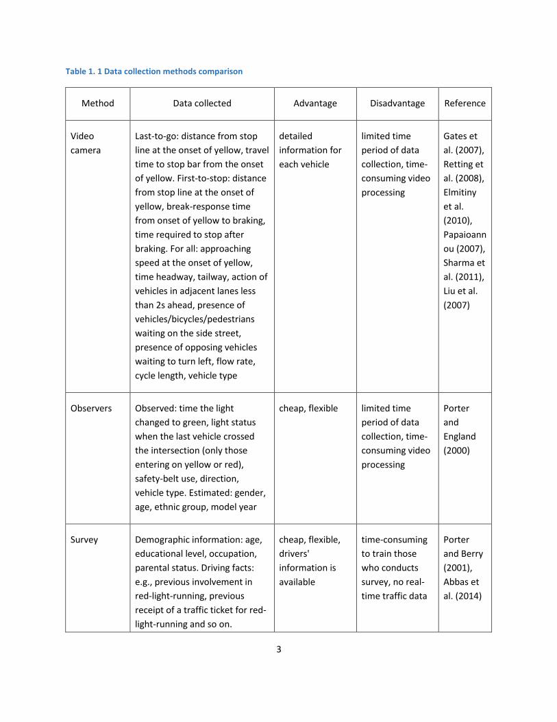
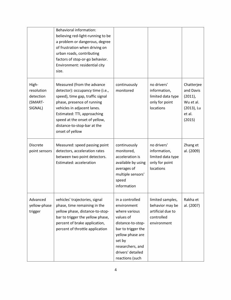
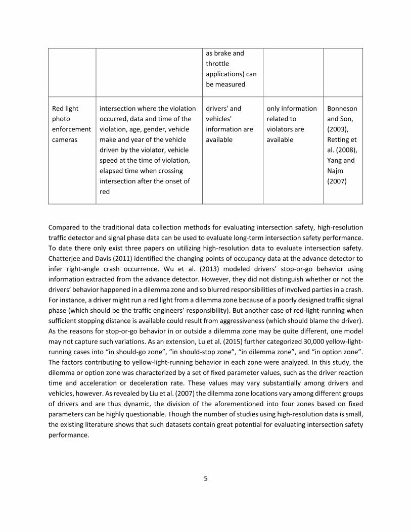
1.2.3 Data Collection Methods
To predict drivers’ behavior while approaching intersections, a variety of data collections methods have
been employed in existing literature. Table 1. 1 summarizes all data collection methods used in the
existing literature. Each method’s advantages and disadvantages are also given.
3
Table 1. 1 Data collection methods comparison
Method Data collected Advantage Disadvantage Reference
Video
camera
Last-to-go: distance from stop
line at the onset of yellow, travel
time to stop bar from the onset
of yellow. First-to-stop: distance
from stop line at the onset of
yellow, break-response time
from onset of yellow to braking,
time required to stop after
braking. For all: approaching
speed at the onset of yellow,
time headway, tailway, action of
vehicles in adjacent lanes less
than 2s ahead, presence of
vehicles/bicycles/pedestrians
waiting on the side street,
presence of opposing vehicles
waiting to turn left, flow rate,
cycle length, vehicle type
detailed
information for
each vehicle
limited time
period of data
collection, time-
consuming video
processing
Gates et
al. (2007),
Retting et
al. (2008),
Elmitiny
et al.
(2010),
Papaioann
ou (2007),
Sharma et
al. (2011),
Liu et al.
(2007)
Observers Observed: time the light
changed to green, light status
when the last vehicle crossed
the intersection (only those
entering on yellow or red),
safety-belt use, direction,
vehicle type. Estimated: gender,
age, ethnic group, model year
cheap, flexible limited time
period of data
collection, time-
consuming video
processing
Porter
and
England
(2000)
Survey Demographic information: age,
educational level, occupation,
parental status. Driving facts:
e.g., previous involvement in
red-light-running, previous
receipt of a traffic ticket for red-
light-running and so on.
cheap, flexible,
drivers'
information is
available
time-consuming
to train those
who conducts
survey, no real-
time traffic data
Porter
and Berry
(2001),
Abbas et
al. (2014)
4
Behavioral information:
believing red-light-running to be
a problem or dangerous, degree
of frustration when driving on
urban roads, contributing
factors of stop-or-go behavior.
Environment: residential city
size.
High-
resolution
detection
(SMART-
SIGNAL)
Measured (from the advance
detector): occupancy time (i.e.,
speed), time gap, traffic signal
phase, presence of running
vehicles in adjacent lanes.
Estimated: TTI, approaching
speed at the onset of yellow,
distance-to-stop-bar at the
onset of yellow
continuously
monitored
no drivers'
information,
limited data type
only for point
locations
Chatterjee
and Davis
(2011),
Wu et al.
(2013), Lu
et al.
(2015)
Discrete
point sensors
Measured: speed passing point
detectors, acceleration rates
between two point detectors.
Estimated: acceleration
continuously
monitored,
acceleration is
available by using
averages of
multiple sensors'
speed
information
no drivers'
information,
limited data type
only for point
locations
Zhang et
al. (2009)
Advanced
yellow-phase
trigger
vehicles' trajectories, signal
phase, time remaining in the
yellow phase, distance-to-stop-
bar to trigger the yellow phase,
percent of brake application,
percent of throttle application
in a controlled
environment
where various
values of
distance-to-stop-
bar to trigger the
yellow phase are
set by
researchers, and
drivers' detailed
reactions (such
limited samples,
behavior may be
artificial due to
controlled
environment
Rakha et
al. (2007)
5
as brake and
throttle
applications) can
be measured
Red light
photo
enforcement
cameras
intersection where the violation
occurred, data and time of the
violation, age, gender, vehicle
make and year of the vehicle
driven by the violator, vehicle
speed at the time of violation,
elapsed time when crossing
intersection after the onset of
red
drivers' and
vehicles'
information are
available
only information
related to
violators are
available
Bonneson
and Son,
(2003),
Retting et
al. (2008),
Yang and
Najm
(2007)
Compared to the traditional data collection methods for evaluating intersection safety, high-resolution
traffic detector and signal phase data can be used to evaluate long-term intersection safety performance.
To date there only exist three papers on utilizing high-resolution data to evaluate intersection safety.
Chatterjee and Davis (2011) identified the changing points of occupancy data at the advance detector to
infer right-angle crash occurrence. Wu et al. (2013) modeled drivers’ stop-or-go behavior using
information extracted from the advance detector. However, they did not distinguish whether or not the
drivers’ behavior happened in a dilemma zone and so blurred responsibilities of involved parties in a crash.
For instance, a driver might run a red light from a dilemma zone because of a poorly designed traffic signal
phase (which should be the traffic engineers’ responsibility). But another case of red-light-running when
sufficient stopping distance is available could result from aggressiveness (which should blame the driver).
As the reasons for stop-or-go behavior in or outside a dilemma zone may be quite different, one model
may not capture such variations. As an extension, Lu et al. (2015) further categorized 30,000 yellow-light-
running cases into “in should-go zone”, “in should-stop zone”, “in dilemma zone”, and “in option zone”.
The factors contributing to yellow-light-running behavior in each zone were analyzed. In this study, the
dilemma or option zone was characterized by a set of fixed parameter values, such as the driver reaction
time and acceleration or deceleration rate. These values may vary substantially among drivers and
vehicles, however. As revealed by Liu et al. (2007) the dilemma zone locations vary among different groups
of drivers and are thus dynamic, the division of the aforementioned into four zones based on fixed
parameters can be highly questionable. Though the number of studies using high-resolution data is small,
the existing literature shows that such datasets contain great potential for evaluating intersection safety
performance.
6
1.3 ORGANIZATION OF THIS REPORT
The report is organized as follows. In chapter 2, we introduce the methodology for identifying red-light-
running (RLR), first-to-stop (FSTP) and yellow-light-running (YLR) events for those intersections with both
stop-bar detectors and entrance detectors. These were located along Trunk Highway (TH55) in Minnesota.
As RLR events can cause conflicts and crashes, the relationship between traffic flow characteristics and
RLR events are studied. Since most intersections along TH55 or TH13 contain neither stop-bar nor
entrance detectors, in chapter 3 we develop a methodology of identifying crossing conflicts at
intersections with advance detectors only. In chapter 4, the Poisson regression is used to link crossing
conflicts and right-angle crashes. The volume-based model is also developed as a comparison. Conclusions
are given in Chapter 5.
7
CHAPTER 2: IDENTIFYING FIRST-TO-STOP (FSTP), YELLOW-
LIGHT RUNNING (YLR), AND RED-LIGHT-RUNNING (RLR) EVENTS
USING STOP BAR AND ENTRANCE DETECTORS
In Chapter 2, we will introduce the methodology of identifying first-to-stop (FSTP), yellow-light-running
(YLR), and red-light-running (RLR) events for those intersections with both stop bar detectors and
entrance detectors located along TH55. As RLR events may cause conflict and crash, the relationship
between traffic flow characteristics and RLR events will be further studied.
Before proceeding, notations which will be used in the rest of the report are listed as follows:
RLR: Red light running event;
YLR: Yellow light running event;
FSTP: First to stop event;
𝐷𝑎: Advance detector;
𝐷𝑠: Stopbar detector;
𝐷𝑒: Entrance detector;
𝑇𝑎/𝑠/𝑒: Timestamp of vehicle actuation at advance/ stop-bar /entrance detector;
𝑡𝑎/𝑠/𝑒: Time headway at advance/stop-bar/entrance detector;
𝑉𝑎: Vehicle speed at advance detector;
𝑉𝑠: Vehicle speed at stopbar detector;
𝑉𝑒: Vehicle speed at entrance detector;
𝑙𝑠𝑒: Distance between the stop-bar detector and the entrance detector;
𝑙𝑠: Distance between the stop-bar detector and the stop bar;
𝑙𝑎: Distance between the advance detector and the stop bar;
𝐿 : Distance between the vehicle and the stop bar;
𝑇𝑌: Start timestamp of the yellow phase;
𝑌𝑎/𝑠/𝑒 : Yellow light running event at advance/ stop-bar /entrance detector;
𝑅𝑎/𝑠/𝑒 : Red light running event at advance/ stop-bar /entrance detector;
8
𝐹𝑎/𝑠/𝑒 : First to stop event at advance/ stop-bar /entrance detector.
Red-light running can potentially cause crashes between vehicles coming from a major and a minor road,
which can thus be used as a surrogate to evaluate intersection safety. Our first task is to identify these
events using SMART-SIGNAL data.
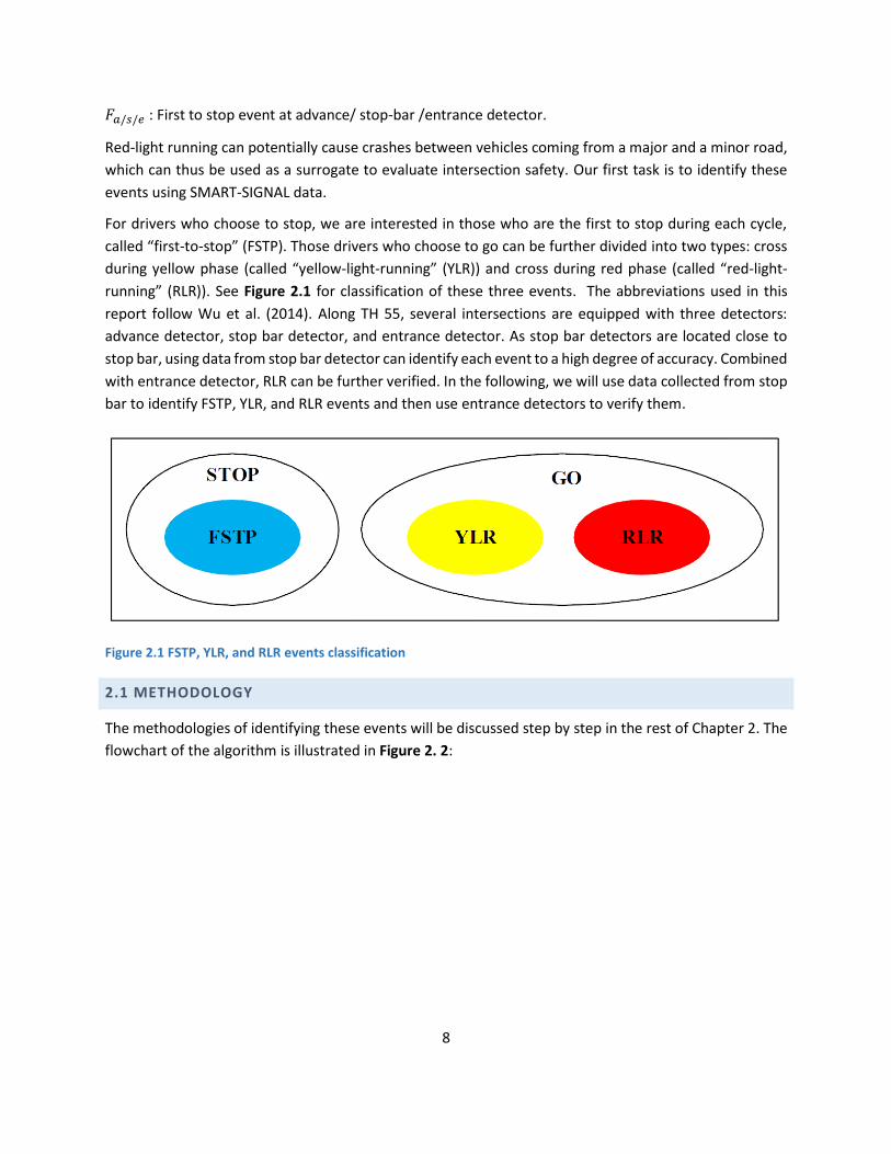
For drivers who choose to stop, we are interested in those who are the first to stop during each cycle,
called “first-to-stop” (FSTP). Those drivers who choose to go can be further divided into two types: cross
during yellow phase (called “yellow-light-running” (YLR)) and cross during red phase (called “red-light-
running” (RLR)). See Figure 2.1 for classification of these three events. The abbreviations used in this
report follow Wu et al. (2014). Along TH 55, several intersections are equipped with three detectors:
advance detector, stop bar detector, and entrance detector. As stop bar detectors are located close to
stop bar, using data from stop bar detector can identify each event to a high degree of accuracy. Combined
with entrance detector, RLR can be further verified. In the following, we will use data collected from stop
bar to identify FSTP, YLR, and RLR events and then use entrance detectors to verify them.
Figure 2.1 FSTP, YLR, and RLR events classification
2.1 METHODOLOGY
The methodologies of identifying these events will be discussed step by step in the rest of Chapter 2. The
flowchart of the algorithm is illustrated in Figure 2. 2:
9
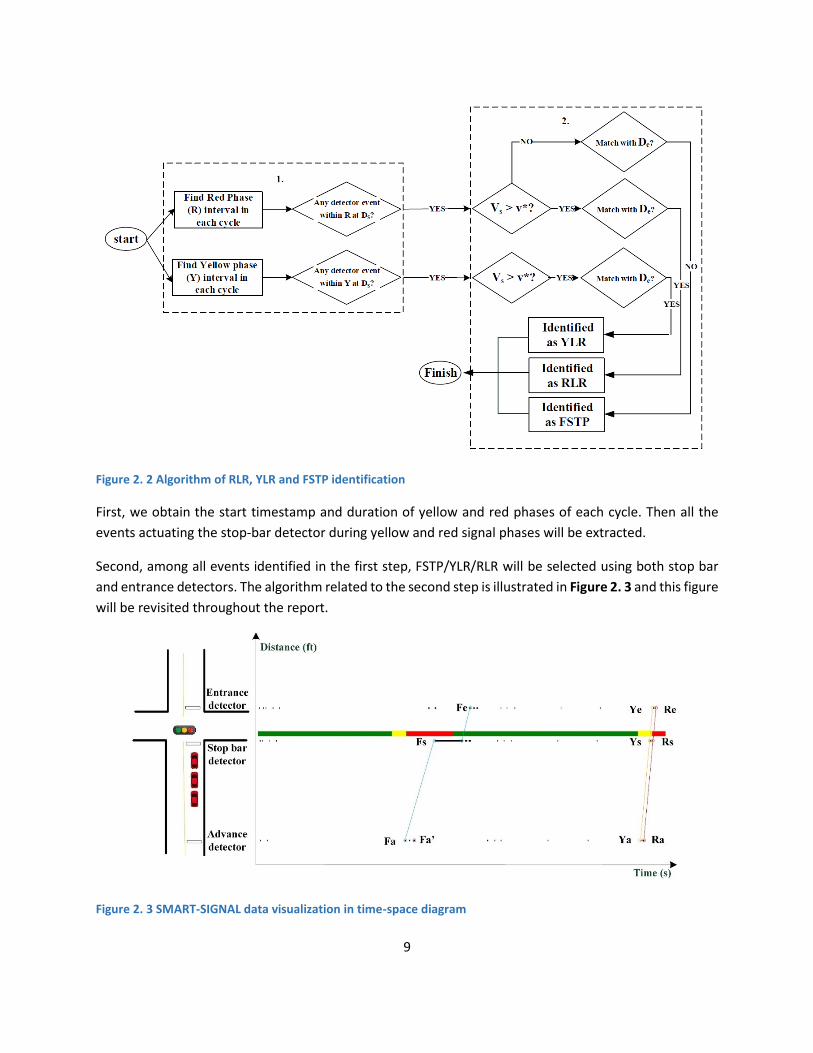
Figure 2. 2 Algorithm of RLR, YLR and FSTP identification
First, we obtain the start timestamp and duration of yellow and red phases of each cycle. Then all the
events actuating the stop-bar detector during yellow and red signal phases will be extracted.
Second, among all events identified in the first step, FSTP/YLR/RLR will be selected using both stop bar
and entrance detectors. The algorithm related to the second step is illustrated in Figure 2. 3 and this figure
will be revisited throughout the report.
Figure 2. 3 SMART-SIGNAL data visualization in time-space diagram
10
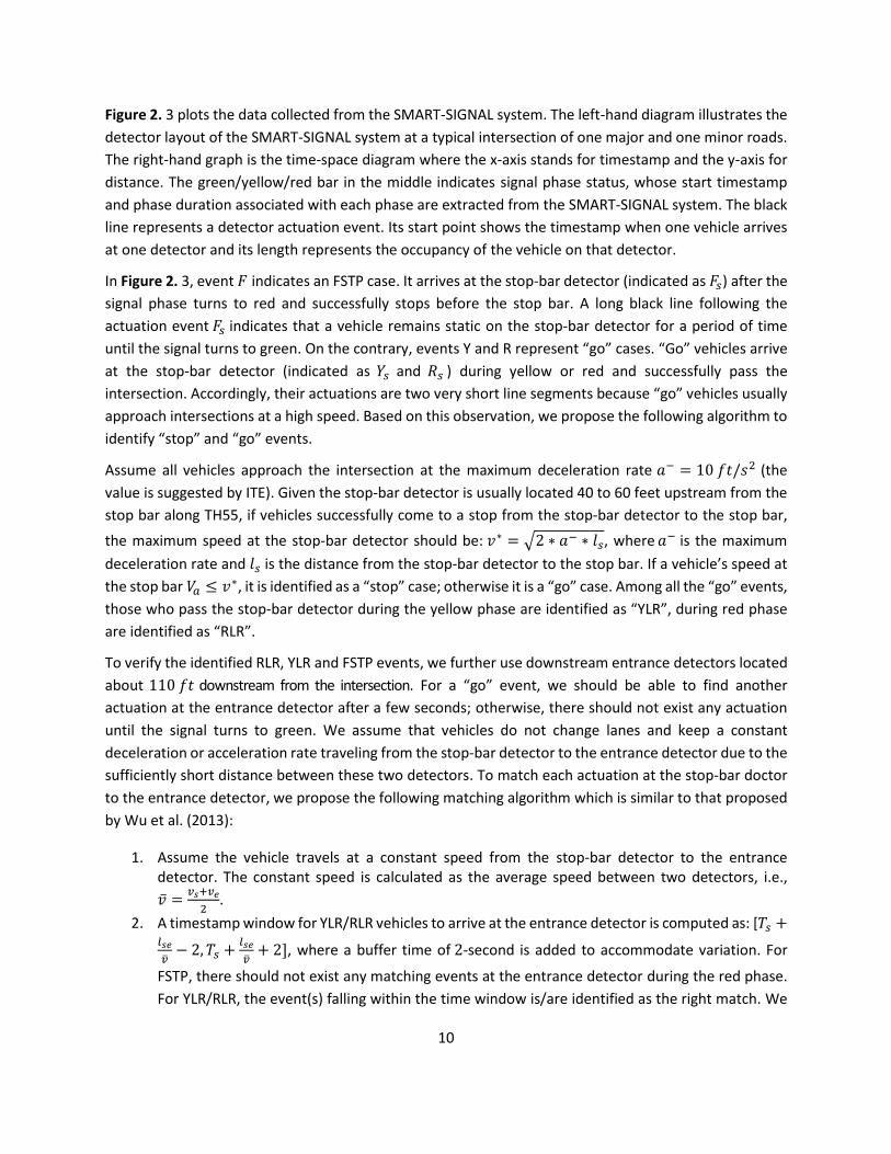
Figure 2. 3 plots the data collected from the SMART-SIGNAL system. The left-hand diagram illustrates the
detector layout of the SMART-SIGNAL system at a typical intersection of one major and one minor roads.
The right-hand graph is the time-space diagram where the x-axis stands for timestamp and the y-axis for
distance. The green/yellow/red bar in the middle indicates signal phase status, whose start timestamp
and phase duration associated with each phase are extracted from the SMART-SIGNAL system. The black
line represents a detector actuation event. Its start point shows the timestamp when one vehicle arrives
at one detector and its length represents the occupancy of the vehicle on that detector.
In Figure 2. 3, event 𝐹 indicates an FSTP case. It arrives at the stop-bar detector (indicated as 𝐹𝑠) after the
signal phase turns to red and successfully stops before the stop bar. A long black line following the
actuation event 𝐹𝑠 indicates that a vehicle remains static on the stop-bar detector for a period of time
until the signal turns to green. On the contrary, events Y and R represent “go” cases. “Go” vehicles arrive
at the stop-bar detector (indicated as 𝑌𝑠 and 𝑅𝑠 ) during yellow or red and successfully pass the
intersection. Accordingly, their actuations are two very short line segments because “go” vehicles usually
approach intersections at a high speed. Based on this observation, we propose the following algorithm to
identify “stop” and “go” events.
Assume all vehicles approach the intersection at the maximum deceleration rate 𝑎− = 10 𝑓𝑡/𝑠2 (the
value is suggested by ITE). Given the stop-bar detector is usually located 40 to 60 feet upstream from the
stop bar along TH55, if vehicles successfully come to a stop from the stop-bar detector to the stop bar,
the maximum speed at the stop-bar detector should be: 𝑣∗ = √2 ∗ 𝑎− ∗ 𝑙𝑠, where 𝑎− is the maximum
deceleration rate and 𝑙𝑠 is the distance from the stop-bar detector to the stop bar. If a vehicle’s speed at
the stop bar 𝑉𝑎 ≤ 𝑣∗, it is identified as a “stop” case; otherwise it is a “go” case. Among all the “go” events,
those who pass the stop-bar detector during the yellow phase are identified as “YLR”, during red phase
are identified as “RLR”.
To verify the identified RLR, YLR and FSTP events, we further use downstream entrance detectors located
about 110 𝑓𝑡 downstream from the intersection. For a “go” event, we should be able to find another
actuation at the entrance detector after a few seconds; otherwise, there should not exist any actuation
until the signal turns to green. We assume that vehicles do not change lanes and keep a constant
deceleration or acceleration rate traveling from the stop-bar detector to the entrance detector due to the
sufficiently short distance between these two detectors. To match each actuation at the stop-bar doctor
to the entrance detector, we propose the following matching algorithm which is similar to that proposed
by Wu et al. (2013):
1. Assume the vehicle travels at a constant speed from the stop-bar detector to the entrance detector. The constant speed is calculated as the average speed between two detectors, i.e.,
�̅� =𝑣𝑠+𝑣𝑒
2.
2. A timestamp window for YLR/RLR vehicles to arrive at the entrance detector is computed as: [𝑇𝑠 +𝑙𝑠𝑒
�̅�− 2, 𝑇𝑠 +
𝑙𝑠𝑒
�̅�+ 2], where a buffer time of 2-second is added to accommodate variation. For
FSTP, there should not exist any matching events at the entrance detector during the red phase.
For YLR/RLR, the event(s) falling within the time window is/are identified as the right match. We
11
should note that selection of 2-second is based on engineering judgement. A longer than 2-
second buffer may result in multiple matches and a shorter than 2-second buffer may lead to no-
match for most cases.
3. When multiple events are matched, we will further compare time headways with its leading vehicle at the stop-bar detector 𝑡𝑠 and at the entrance detector 𝑡𝑒 respectively across all matched pairs. The pair which has the closest headways at two detectors will be picked. Mathematically,
𝑖∗ = 𝑚𝑖𝑛𝑖|𝑡𝑠 − 𝑡𝑒𝑖 |, where 𝑖 is the index of the potentially identified cases.
In Error! Reference source not found., there does not exist a match 𝐹𝑒 at the entrance detector for 𝐹𝑠 until a
fter the signal phase turns to green. Cases 𝑌𝑠, 𝑅𝑠 are both matched to entrance actuations 𝑌𝑒 , 𝑅𝑒
respectively. Therefore we can confirm that they are “go” events.
Among three events, RLR may potentially cause crossing conflicts and crash, so we will analyze its
relationship with traffic flow characteristics at one intersection along TH55.
2.2 RLR EVENTS
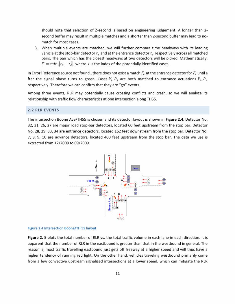
The intersection Boone Ave/TH55 is chosen and its detector layout is shown in Figure 2.4. Detector No.
32, 31, 26, 27 are major road stop-bar detectors, located 60 feet upstream from the stop bar. Detector
No. 28, 29, 33, 34 are entrance detectors, located 162 feet downstream from the stop bar. Detector No.
7, 8, 9, 10 are advance detectors, located 400 feet upstream from the stop bar. The data we use is
extracted from 12/2008 to 09/2009.
Figure 2.4 Intersection Boone/TH 55 layout
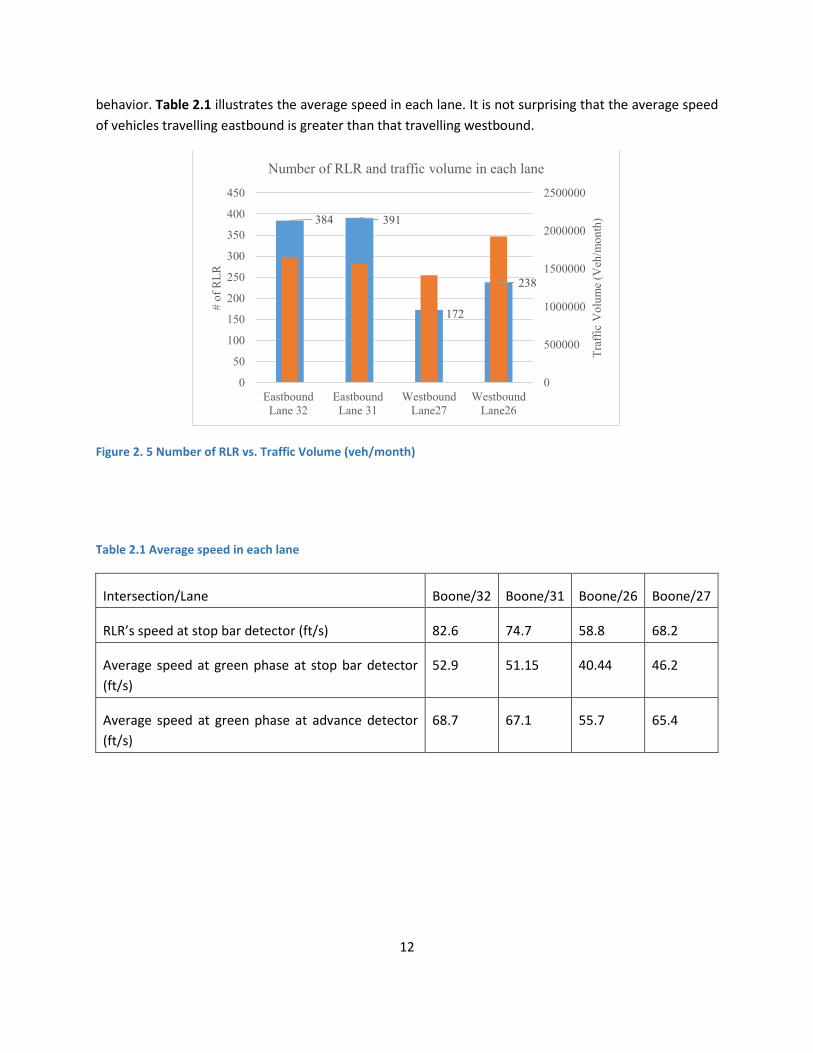
Figure 2. 5 plots the total number of RLR vs. the total traffic volume in each lane in each direction. It is
apparent that the number of RLR in the eastbound is greater than that in the westbound in general. The
reason is, most traffic travelling eastbound just gets off freeway at a higher speed and will thus have a
higher tendency of running red light. On the other hand, vehicles traveling westbound primarily come
from a few convective upstream signalized intersections at a lower speed, which can mitigate the RLR
12
behavior. Table 2.1 illustrates the average speed in each lane. It is not surprising that the average speed
of vehicles travelling eastbound is greater than that travelling westbound.
Figure 2. 5 Number of RLR vs. Traffic Volume (veh/month)
384 391
172
238
0
500000
1000000
1500000
2000000
2500000
0
50
100
150
200
250
300
350
400
450
Eastbound
Lane 32
Eastbound
Lane 31
Westbound
Lane27
Westbound
Lane26
Tra
ffic
Vo
lum
e (V
eh/m
on
th)
# o
f R
LR
Number of RLR and traffic volume in each lane
Table 2.1 Average speed in each lane
Intersection/Lane Boone/32 Boone/31 Boone/26 Boone/27
RLR’s speed at stop bar detector (ft/s) 82.6 74.7 58.8 68.2
Average speed at green phase at stop bar detector
(ft/s)
52.9 51.15 40.44 46.2
Average speed at green phase at advance detector
(ft/s)
68.7 67.1 55.7 65.4

13
(a)
(b)
Figure 2. 6 Number of RLR vs. traffic volume over the time of day for (a) westbound and (b) eastbound
1 2 3 4 5 6 7 8 9 10 11 12 13 14 15 16 17 18 19 20 21 22 23 24
0
2000
4000
6000
8000
10000
12000
0
0.5
1
1.5
2
2.5
3
3.5
4
4.5
Tra
ffic
Vo
lum
e (V
eh/d
ay)
# o
f R
LR
Time of day
# of RLR and volume in the time of day (Eastbound)
# of RLR volume
1 2 3 4 5 6 7 8 9 10 11 12 13 14 15 16 17 18 19 20 21 22 23 24
0
2000
4000
6000
8000
10000
12000
0
0.5
1
1.5
2
Tra
ffic
Vo
lum
e (V
eh/d
ay)
# o
f R
LR
Time of day
# of RLR and traffic volume in the time of day (Westbound)
# of RLR volume
14
0
2000
4000
6000
8000
10000
12000
14000
16000
18000
0
0.5
1
1.5
2
2.5
3
3.5
4
4.5
5
Dai
ly T
raff
ic V
olu
me
(veh
/day
)
# o
f d
aily
RL
R
Month
# of average RLR and volume in each month(Eastbound)
# of RLR volume
(a)
(b)
Figure 2. 7 Number of RLR vs. daily traffic volume in each month for (a) westbound and (b) eastbound
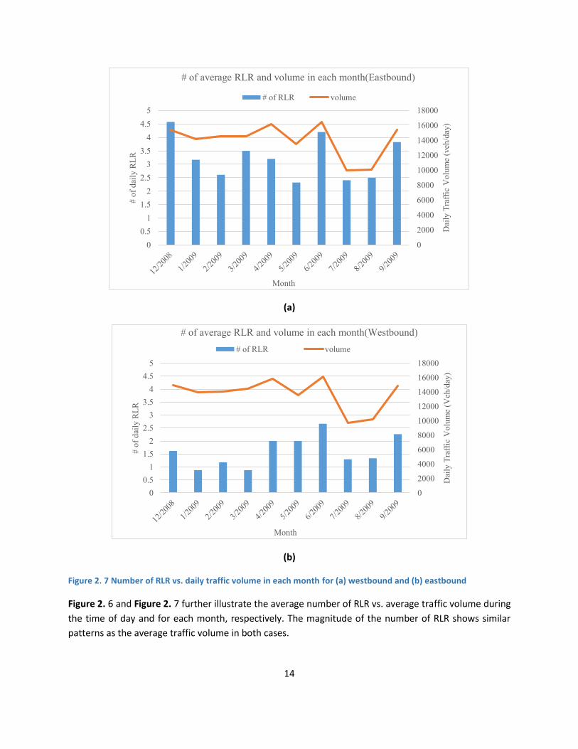
Figure 2. 6 and Figure 2. 7 further illustrate the average number of RLR vs. average traffic volume during
the time of day and for each month, respectively. The magnitude of the number of RLR shows similar
patterns as the average traffic volume in both cases.
0
2000
4000
6000
8000
10000
12000
14000
16000
18000
0
0.5
1
1.5
2
2.5
3
3.5
4
4.5
5
Dai
ly T
raff
ic V
olu
me
(Veh
/day
)
# o
f d
aily
RL
R
Month
# of average RLR and volume in each month(Westbound)
# of RLR volume
15
2.3 MODELING STOP-OR-GO BEHAVIOR USING ADVANCE DETECTOR DATA
Ideally, RLR can be used as a surrogate to evaluate intersection safety. However, not all intersections are
equipped with stop-bar detectors, which prevents us from accurately identifying RLR events. Therefore,
we have to use another surrogate, i.e., crossing conflict, for the intersection safety evaluation purpose.
As almost every intersection contains one advance detector, in this chapter, we will aim to develop a
methodology of predicting drivers’ stop-or-go behavior using only advance detector data. After “go”
events are identified along both major and minor roads, we will be able to capture a crossing conflict.
To ensure that the developed model can capture those “go” events to a certain degree of accuracy, we
will have to first focus on those intersections equipped with stop bar and entrance detectors, which will
help train a model using the actual “go” events. Specifically, we will extract relevant information of all
“go” and “stop” events (identified with the help of stop bar and entrance detectors) recorded at advance
detectors. Then a statistical model will be trained using the available information. It will then be used for
predicting “go” events at intersections where only advance detectors are equipped.
2.3.1 Matching Events to Advance Detectors and Data Extraction
After FSTP/YLR/RLR events are identified at the stop-bar detector and verified by the entrance detector,
illustrated in Section 2.1, now we need to match them to the advance detector. Matching YLR/RLR events
from the stop-bar detector to the advance detector is the same as matching them to the entrance
detector. Matching FSTP events to the advance detector, however, is different from matching them to the
entrance detector. If we use the same algorithm as introduced in Section 2.1, there will be mismatches.
For example, in Figure 2. 3, while trying to find the match 𝐹𝑎 for 𝐹𝑠, if a 2-second time-window is defined,
event 𝐹𝑎′ will be recognized as the match. However, the actual one is 𝐹𝑎. The trajectory connecting 𝐹𝑎 and
𝐹𝑠 is not as steep as that connecting 𝐹𝑎′ and 𝐹𝑠, meaning the vehicle is actually decelerating. The reason
for mismatching is that the traffic dynamic between the advance detector and the stop-bar detector
spanning 400 feet is complicated during the yellow phase due to queuing built-up. In addition, stopping
vehicles’ deceleration manifests great variations in terms of when and where to start to decelerate and
where to stop. We found out that such mismatches are quite common for FSTP events and can further
impair the subsequent analysis. Therefore, to match FSTP cases to the advance detector more accurately,
we will match the last “go” event (i.e., the vehicle right in front of the FSTP). Because “go” vehicles usually
keep relatively constant speed or accelerate rate and do not show significant variation in speed compared
to stopping vehicles. After the last “go” event is matched, FSTP is the one following the matched “go”
event.
The information extracted from the advance detector can be divided into two types: direct information
and derived information (e.g., speed and distance-to-stop bar at the onset of yellow phase). Table 2. 2
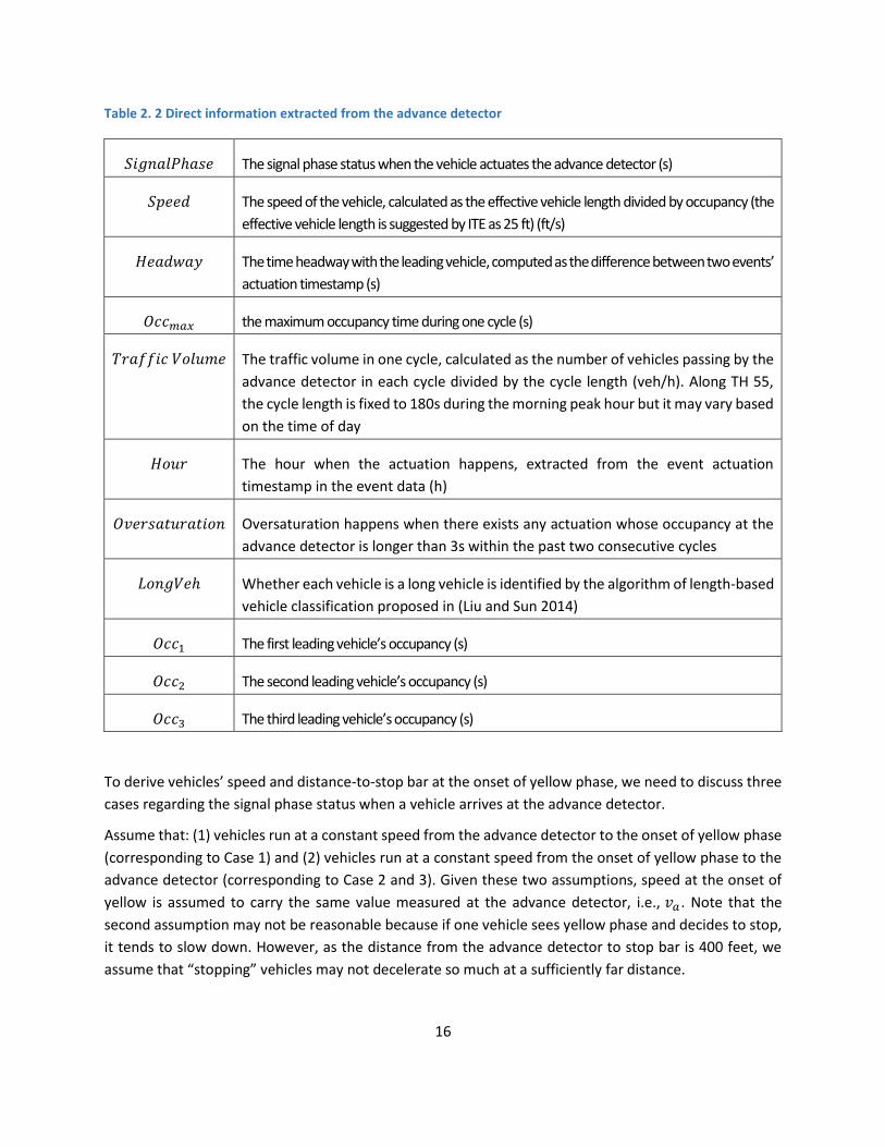
lists all information directly extracted from the advance detector.
16
Table 2. 2 Direct information extracted from the advance detector
𝑆𝑖𝑔𝑛𝑎𝑙𝑃ℎ𝑎𝑠𝑒 The signal phase status when the vehicle actuates the advance detector (s)
𝑆𝑝𝑒𝑒𝑑 The speed of the vehicle, calculated as the effective vehicle length divided by occupancy (the
effective vehicle length is suggested by ITE as 25 ft) (ft/s)
𝐻𝑒𝑎𝑑𝑤𝑎𝑦 The time headway with the leading vehicle, computed as the difference between two events’
actuation timestamp (s)
𝑂𝑐𝑐𝑚𝑎𝑥 the maximum occupancy time during one cycle (s)
𝑇𝑟𝑎𝑓𝑓𝑖𝑐 𝑉𝑜𝑙𝑢𝑚𝑒 The traffic volume in one cycle, calculated as the number of vehicles passing by the
advance detector in each cycle divided by the cycle length (veh/h). Along TH 55,
the cycle length is fixed to 180s during the morning peak hour but it may vary based
on the time of day
𝐻𝑜𝑢𝑟 The hour when the actuation happens, extracted from the event actuation
timestamp in the event data (h)
𝑂𝑣𝑒𝑟𝑠𝑎𝑡𝑢𝑟𝑎𝑡𝑖𝑜𝑛 Oversaturation happens when there exists any actuation whose occupancy at the
advance detector is longer than 3s within the past two consecutive cycles
𝐿𝑜𝑛𝑔𝑉𝑒ℎ Whether each vehicle is a long vehicle is identified by the algorithm of length-based
vehicle classification proposed in (Liu and Sun 2014)
𝑂𝑐𝑐1 The first leading vehicle’s occupancy (s)
𝑂𝑐𝑐2 The second leading vehicle’s occupancy (s)
𝑂𝑐𝑐3 The third leading vehicle’s occupancy (s)
To derive vehicles’ speed and distance-to-stop bar at the onset of yellow phase, we need to discuss three
cases regarding the signal phase status when a vehicle arrives at the advance detector.
Assume that: (1) vehicles run at a constant speed from the advance detector to the onset of yellow phase
(corresponding to Case 1) and (2) vehicles run at a constant speed from the onset of yellow phase to the
advance detector (corresponding to Case 2 and 3). Given these two assumptions, speed at the onset of
yellow is assumed to carry the same value measured at the advance detector, i.e., 𝑣𝑎 . Note that the
second assumption may not be reasonable because if one vehicle sees yellow phase and decides to stop,
it tends to slow down. However, as the distance from the advance detector to stop bar is 400 feet, we
assume that “stopping” vehicles may not decelerate so much at a sufficiently far distance.

17
Figure 2. 8 Three scenarios when a vehicle arrives at the advance detector
Case 1: the signal phase is green when the vehicle arrives at the advance detector:
Case 2: the signal phase is yellow when the vehicle arrives at the advance detector:
Case 3: the signal phase is red when the vehicle arrives at the advance detector:
Define
𝑃ℎ𝑎𝑠𝑒 𝑠𝑡𝑎𝑡𝑢𝑠 = 𝑇𝑎 − 𝑇𝑌={
< 0, 𝑖𝑓 𝑎𝑟𝑟𝑖𝑣𝑒𝑠 𝑎𝑡 𝑡ℎ𝑒 𝐷𝑎. 𝑑𝑢𝑟𝑖𝑛𝑔 𝑔𝑟𝑒𝑒𝑛 ,= 0, 𝑖𝑓 𝑎𝑟𝑟𝑖𝑣𝑒𝑠 𝑎𝑡 𝑡ℎ𝑒 𝐷𝑎 𝑎𝑡 𝑡ℎ𝑒 𝑜𝑛𝑠𝑒𝑡 𝑜𝑓 𝑦𝑒𝑙𝑙𝑜𝑤 𝑝ℎ𝑎𝑠𝑒,
∈ (0, 𝑌], 𝑖𝑓 𝑎𝑟𝑟𝑖𝑣𝑒𝑠 𝑎𝑡 𝑡ℎ𝑒𝐷𝑎 𝑑𝑢𝑟𝑖𝑛𝑔 𝑦𝑒𝑙𝑙𝑜𝑤 𝑝ℎ𝑎𝑠𝑒,> 𝑌, 𝑖𝑓 𝑎𝑟𝑟𝑖𝑣𝑒𝑠 𝑎𝑡 𝑡ℎ𝑒 𝐷𝑎 𝑑𝑢𝑟𝑖𝑛𝑔 𝑟𝑒𝑑 𝑝ℎ𝑎𝑠𝑒.
(2)
The distance-to-stop-bar 𝐿 at the onset of yellow phase can thus be estimated as:
𝐿 = 𝐿𝑎 + 𝑝 ∗ 𝑣𝑎 . (3)
𝑇𝑎 < 𝑇𝑌 𝐿 < 𝑙𝑎
𝐿 > 𝑙𝑎
𝐿 > 𝑙𝑎
𝑇𝑌 < 𝑇𝑎 ≤ 𝑇𝑌 + 𝑌
𝑇𝑎 > 𝑇𝑌 + 𝑌

18
Time-to-intersection (TTI) is defined as the time one vehicle takes to reach the intersection from the onset
of yellow phase. It is computed as:
𝑇𝑇𝐼 =𝐿
𝑣𝑎. (4)
From the SMART-SIGNAL system, we extract RLR/YLR/FSTP events using the algorithm proposed in Section
2. The parameters associated to each event, such as distance to the stop bar at the onset of yellow phase,
speed, are directly or indirectly extracted from the advance detector.
We will now use the intersection Rhode Island/TH55 to illustrate how high-resolution data can help
identify dilemma/option zone boundaries. The reason we pick this intersection is that it contains three
legs, i.e., there exists no right-turn. Accordingly, the proposed matching algorithm will work more
accurately and events mismatch will be unlikely to happen. The link between two intersections is 752 ft
long and its speed limit is 55mi/h. The detector deployment layout is shown in Figure 2. 9. Detector No.
16, 17, 13, 12 are stop-bar detectors, located on the main road 10 feet upstream from the stop bar.
Detector No. 14, 15, 18, 19 are entrance detectors, deployed 142 feet downstream from the stop bar.
Detector No. 1, 2, 9, 10 are advance detectors, located 375 feet upstream from the stop bar.
Figure 2. 9 Intersection Rhode Island/TH 55 layout
Table 2. 3 shows the detailed description of the data we use at intersection Rhode Island/TH55 to model
and predict stop-or-go behavior.
Time period RLR events YLR events FSTP events
Training dataset Nov. May. Jul. 228 8454 7575
Training dataset within
dilemma or option zone
Nov. May. Jul. 122 3905 1335

19
Validation dataset Aug. Sep. 82 3555 2994
Validation dataset within
dilemma or option zone
Aug. Sep. 43 1632 520
Table 2. 3 Description of datasets at Rhode Island/TH55 intersection
We choose not to use the data from the month of December to April to remove the snow effects. Data of
June 2009 is incomplete, so it is also excluded from the analysis.
2.3.2 Training a Stop-Or-Go Model
The logistic regression is used to model drivers’ stop-or-go behavior in face of yellow with the extracted
information from the advance detector (listed in Table 2. 2):
log (𝑃(𝑔𝑜)
𝑃(𝑠𝑡𝑜𝑝)) = 𝛽0 + 𝛽1 𝑆𝑖𝑔𝑛𝑎𝑙𝑃ℎ𝑎𝑠𝑒 + 𝛽2𝑆𝑝𝑒𝑒𝑑 + 𝛽3𝐻𝑒𝑎𝑑𝑤𝑎𝑦 + 𝛽4 log(𝑂𝑐𝑐𝑚𝑎𝑥) + 𝛽5𝐹𝑙𝑜𝑤 +
𝛽6𝐻𝑜𝑢𝑟 + 𝛽7𝑂𝑣𝑒𝑟𝑠𝑎𝑡𝑢𝑟𝑎𝑡𝑖𝑜𝑛 + 𝛽8𝐿𝑜𝑛𝑔𝑉𝑒ℎ + 𝛽9 log(𝑂𝑐𝑐1) + 𝛽10 log(𝑂𝑐𝑐2) + 𝛽11 log(𝑂𝑐𝑐3)
(5)
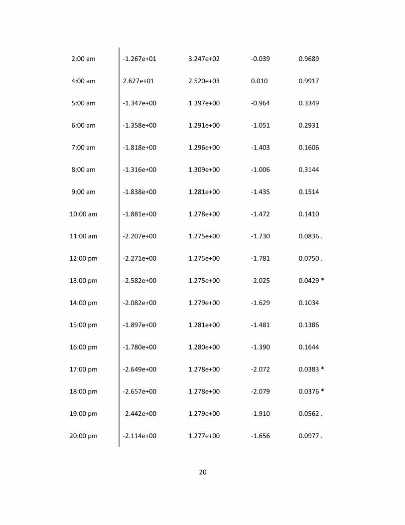
The estimated coefficients of logistic regression are listed in Table 2. 4.
Table 2. 4 Coefficients of logistic regression
Coefficients Estimate Std. Error Z value Pr(>|z|)
(Intercept) -2.748e+00 1.343e+00 -2.047 0.0407 *
Signal Phase -1.451e+00 5.181e-02 -28.007 <2e-16 ***
Speed 8.024e-02 5.417e-03 14.812 <2e-16 ***
Headway -1.537e-02 2.467e-03 -6.230 4.68e-10 ***
𝑂𝑐𝑐𝑚𝑎𝑥 -5.297e-01 1.310e-01 -4.043 5.28e-05 ***
Traffic Volume 4.030e-04 1.871e-04 2.154 0.0313 *
1:00 am -1.415e+01 3.247e+02 -0.044 0.9652
20
2:00 am -1.267e+01 3.247e+02 -0.039 0.9689
4:00 am 2.627e+01 2.520e+03 0.010 0.9917
5:00 am -1.347e+00 1.397e+00 -0.964 0.3349
6:00 am -1.358e+00 1.291e+00 -1.051 0.2931
7:00 am -1.818e+00 1.296e+00 -1.403 0.1606
8:00 am -1.316e+00 1.309e+00 -1.006 0.3144
9:00 am -1.838e+00 1.281e+00 -1.435 0.1514
10:00 am -1.881e+00 1.278e+00 -1.472 0.1410
11:00 am -2.207e+00 1.275e+00 -1.730 0.0836 .
12:00 pm -2.271e+00 1.275e+00 -1.781 0.0750 .
13:00 pm -2.582e+00 1.275e+00 -2.025 0.0429 *
14:00 pm -2.082e+00 1.279e+00 -1.629 0.1034
15:00 pm -1.897e+00 1.281e+00 -1.481 0.1386
16:00 pm -1.780e+00 1.280e+00 -1.390 0.1644
17:00 pm -2.649e+00 1.278e+00 -2.072 0.0383 *
18:00 pm -2.657e+00 1.278e+00 -2.079 0.0376 *
19:00 pm -2.442e+00 1.279e+00 -1.910 0.0562 .
20:00 pm -2.114e+00 1.277e+00 -1.656 0.0977 .
21
21:00 pm -2.873e+00 1.299e+00 -2.212 0.0270 *
22:00 pm -2.462e+00 1.319e+00 -1.866 0.0620 .
23:00 pm -1.627e+00 1.447e+00 -1.124 0.2609
Oversaturation 1.139e+00 1.183e+00 0.962 0.3359
Long vehicle -4.165e-01 3.435e-01 -1.212 0.2253
Oc𝑐1 -1.437e-01 1.661e-01 -0.865 0.3868
Occ2 -7.585e-03 1.352e-01 -0.056 0.9553
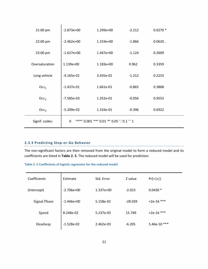
Occ3 -5.209e-02 1.316e-01 -0.396 0.6922
Signif. codes: 0 ‘***’ 0.001 ‘**’ 0.01 ‘*’ 0.05 ‘.’ 0.1 ‘ ’ 1
2.3.3 Predicting Stop-or-Go Behavior
The non-significant factors are then removed from the original model to form a reduced model and its
coefficients are listed in Table 2. 5. The reduced model will be used for prediction.
Table 2. 5 Coefficients of logistic regression for the reduced model
Coefficients Estimate Std. Error Z value Pr(>|z|)
(Intercept) -2.706e+00 1.337e+00 -2.023 0.0430 *
Signal Phase -1.446e+00 5.158e-02 -28.039 <2e-16 ***
Speed 8.248e-02 5.237e-03 15.749 <2e-16 ***
Headway -1.528e-02 2.462e-03 -6.205 5.46e-10 ***
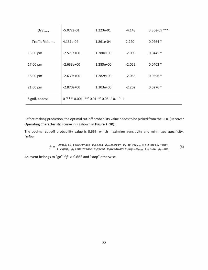
22
𝑂𝑐𝑐𝑚𝑎𝑥 -5.072e-01 1.223e-01 -4.148 3.36e-05 ***
Traffic Volume 4.131e-04 1.861e-04 2.220 0.0264 *
13:00 pm -2.571e+00 1.280e+00 -2.009 0.0445 *
17:00 pm -2.633e+00 1.283e+00 -2.052 0.0402 *
18:00 pm -2.639e+00 1.282e+00 -2.058 0.0396 *
21:00 pm -2.870e+00 1.303e+00 -2.202 0.0276 *
Signif. codes: 0 ‘***’ 0.001 ‘**’ 0.01 ‘*’ 0.05 ‘.’ 0.1 ‘ ’ 1
Before making prediction, the optimal cut-off probability value needs to be picked from the ROC (Receiver
Operating Characteristic) curve in R (shown in Figure 2. 10).
The optimal cut-off probability value is 0.665, which maximizes sensitivity and minimizes specificity.
Define
�̂� =𝑒𝑥𝑝(𝛽0+𝛽1 𝑌𝑒𝑙𝑙𝑜𝑤𝑃ℎ𝑎𝑠𝑒+𝛽2𝑆𝑝𝑒𝑒𝑑+𝛽3𝐻𝑒𝑎𝑑𝑤𝑎𝑦+𝛽4 log(𝑂𝑐𝑐𝑚𝑎𝑥)+𝛽5𝐹𝑙𝑜𝑤+𝛽6𝐻𝑜𝑢𝑟)
1−𝑒𝑥𝑝(𝛽0+𝛽1 𝑌𝑒𝑙𝑙𝑜𝑤𝑃ℎ𝑎𝑠𝑒+𝛽2𝑆𝑝𝑒𝑒𝑑+𝛽3𝐻𝑒𝑎𝑑𝑤𝑎𝑦+𝛽4 log(𝑂𝑐𝑐𝑚𝑎𝑥)+𝛽5𝐹𝑙𝑜𝑤+𝛽6𝐻𝑜𝑢𝑟) (6)
An event belongs to “go” if �̂� > 0.665 and “stop” otherwise.
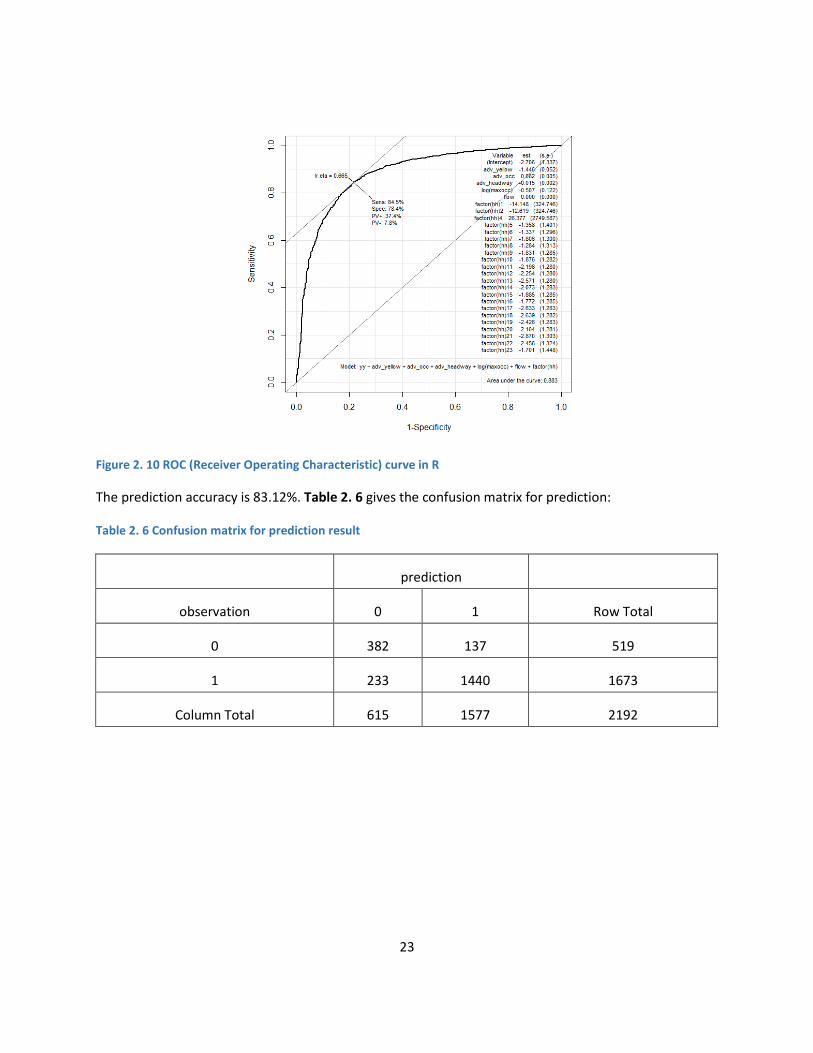
23
Figure 2. 10 ROC (Receiver Operating Characteristic) curve in R
The prediction accuracy is 83.12%. Table 2. 6 gives the confusion matrix for prediction:
Table 2. 6 Confusion matrix for prediction result
prediction
observation 0 1 Row Total
0 382 137 519
1 233 1440 1673
Column Total 615 1577 2192
24
CHAPTER 3: IDENTIFYING CROSSING CONFLICT ADVANCE
DETECTORS
At a signalized intersection, red light running may incur crossing conflicts, which will likely lead to right-
angle crashes. Accordingly, crossing conflicts can be employed as a surrogate for signalized intersection
safety evaluation. In chapter 3, we will develop a cost-effective way of predicting crossing conflicts using
high-resolution traffic signal data collected from the SMART-Signal systems.
3.1 METHODOLOGY
The stop-or-go prediction model presented in chapter 2 predicts whether a vehicle stops or goes in face
of red phase. If it crosses the intersection during the red phase, we will then check whether there is any
vehicle coming from the minor road during that time interval. If yes, a potential crossing conflict will be
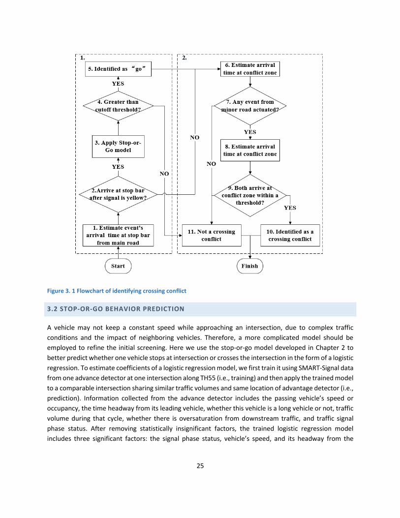
identified. Therefore identifying crossing conflict events includes two steps: (1) identifying “go” events
during the red phase on both main and minor roads, and (2) calculating crossing conflicts within conflict
zones. The flowchart of these two steps is illustrated in Figure 3. 1.
We first briefly describe a process to predict vehicle’s stop-or-go behavior, using the event based traffic
data. Based on actuation event at an advance detector, the process will predict whether the vehicle will
stop or go at the downstream stop bar. Here, we will only focus on those “go” vehicles, which may incur
crossing conflicts.
As an initial screening, we first calculate each vehicle’s arrival time to an intersection by assuming that it
travels at a constant speed and does not change lanes. So the arrival time equals to the distance between
advance detector and stop-bar detector divided by its speed at advance detector. Define a time window:
[𝑇𝑅 − 𝑌, 𝑇𝑅 + 𝑌], where 𝑇𝑅 is the red phase start timestamp and Y is the yellow phase duration, i.e., 5.5
second, rounding up to the integer. If the arrival time at the stop bar is within the time window, the event
is identified as a potential “go” event. This event will be further checked by applying a “stop or go” model
in the next step.
25
Figure 3. 1 Flowchart of identifying crossing conflict
3.2 STOP-OR-GO BEHAVIOR PREDICTION
A vehicle may not keep a constant speed while approaching an intersection, due to complex traffic
conditions and the impact of neighboring vehicles. Therefore, a more complicated model should be
employed to refine the initial screening. Here we use the stop-or-go model developed in Chapter 2 to
better predict whether one vehicle stops at intersection or crosses the intersection in the form of a logistic
regression. To estimate coefficients of a logistic regression model, we first train it using SMART-Signal data
from one advance detector at one intersection along TH55 (i.e., training) and then apply the trained model
to a comparable intersection sharing similar traffic volumes and same location of advantage detector (i.e.,
prediction). Information collected from the advance detector includes the passing vehicle’s speed or
occupancy, the time headway from its leading vehicle, whether this vehicle is a long vehicle or not, traffic
volume during that cycle, whether there is oversaturation from downstream traffic, and traffic signal
phase status. After removing statistically insignificant factors, the trained logistic regression model
includes three significant factors: the signal phase status, vehicle’s speed, and its headway from the
26
leading vehicle. The phase status is defined in Equation 2. With the trained model, the probability of “go”
is calculated by Equation 7:
𝑃(𝑔𝑜) = �̂� =𝑒𝑥𝑝(𝛽0+𝛽1 𝑃ℎ𝑎𝑠𝑒𝑆𝑡𝑎𝑡𝑢𝑠+𝛽2𝑆𝑝𝑒𝑒𝑑+𝛽3𝐻𝑒𝑎𝑑𝑤𝑎𝑦)
1+𝑒𝑥𝑝(𝛽0+𝛽1 𝑃ℎ𝑎𝑠𝑒𝑆𝑡𝑎𝑡𝑢𝑠+𝛽2𝑆𝑝𝑒𝑒𝑑+𝛽3𝐻𝑒𝑎𝑑𝑤𝑎𝑦) (7)
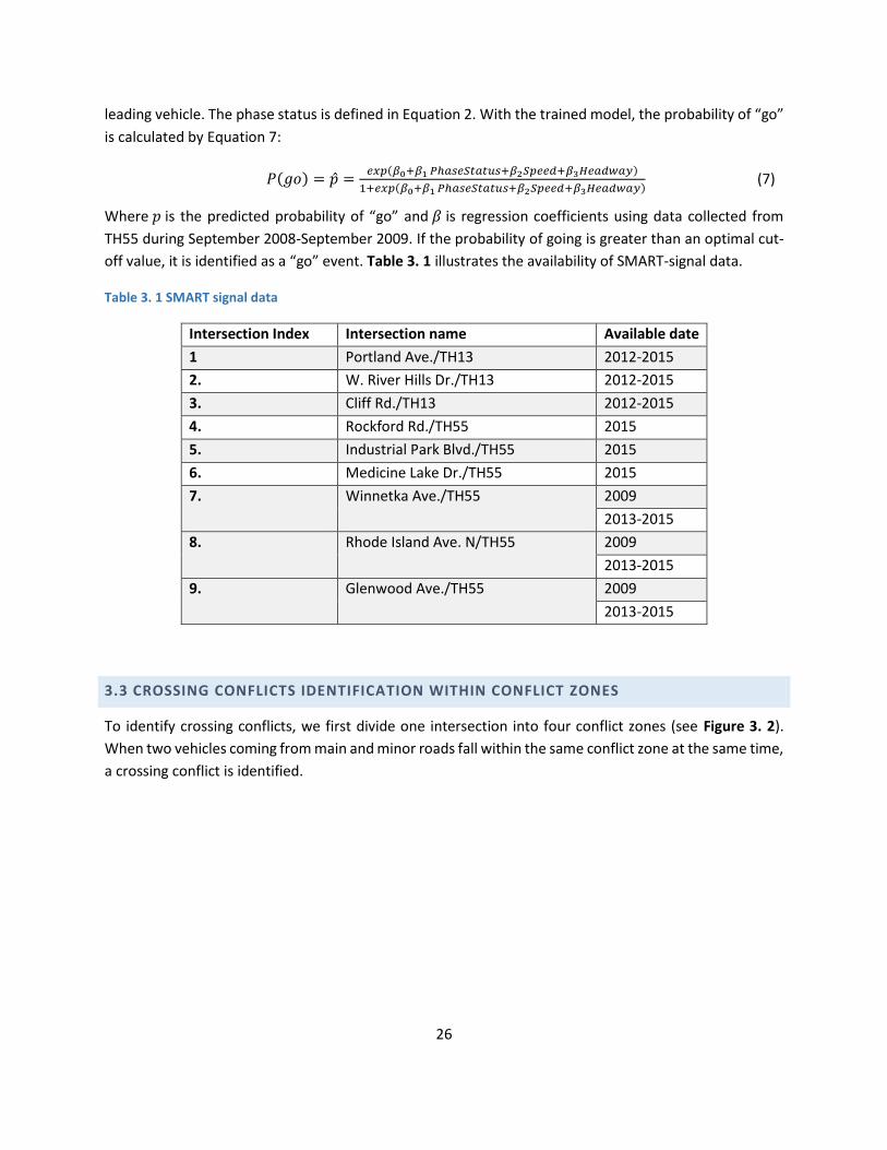
Where 𝑝 is the predicted probability of “go” and 𝛽 is regression coefficients using data collected from
TH55 during September 2008-September 2009. If the probability of going is greater than an optimal cut-
off value, it is identified as a “go” event. Table 3. 1 illustrates the availability of SMART-signal data.
Table 3. 1 SMART signal data
Intersection Index Intersection name Available date
1 Portland Ave./TH13 2012-2015
2. W. River Hills Dr./TH13 2012-2015
3. Cliff Rd./TH13 2012-2015
4. Rockford Rd./TH55 2015
5. Industrial Park Blvd./TH55 2015
6. Medicine Lake Dr./TH55 2015
7. Winnetka Ave./TH55 2009
2013-2015
8. Rhode Island Ave. N/TH55 2009
2013-2015
9. Glenwood Ave./TH55 2009
2013-2015
3.3 CROSSING CONFLICTS IDENTIFICATION WITHIN CONFLICT ZONES
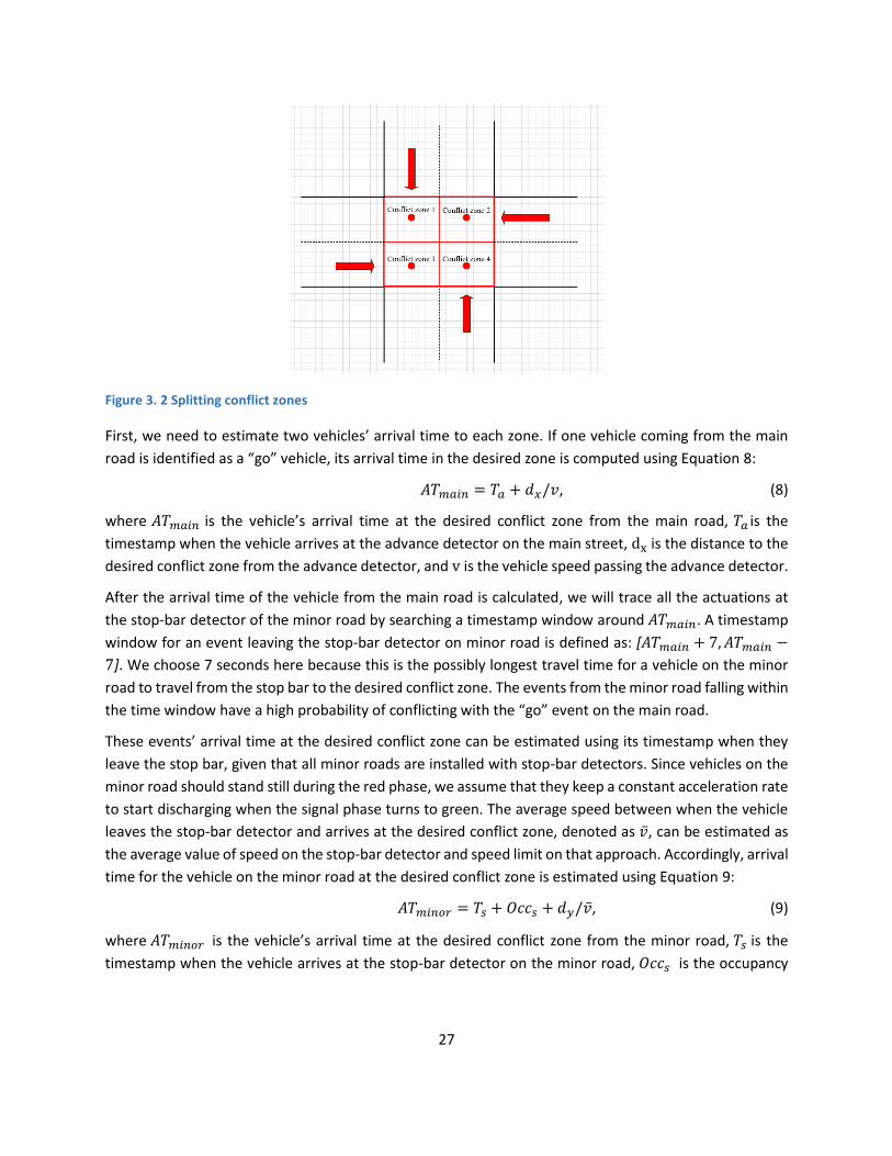
To identify crossing conflicts, we first divide one intersection into four conflict zones (see Figure 3. 2).
When two vehicles coming from main and minor roads fall within the same conflict zone at the same time,
a crossing conflict is identified.
27
Figure 3. 2 Splitting conflict zones
First, we need to estimate two vehicles’ arrival time to each zone. If one vehicle coming from the main
road is identified as a “go” vehicle, its arrival time in the desired zone is computed using Equation 8:
𝐴𝑇𝑚𝑎𝑖𝑛 = 𝑇𝑎 + 𝑑𝑥/𝑣, (8)
where 𝐴𝑇𝑚𝑎𝑖𝑛 is the vehicle’s arrival time at the desired conflict zone from the main road, 𝑇𝑎 is the
timestamp when the vehicle arrives at the advance detector on the main street, dx is the distance to the
desired conflict zone from the advance detector, and v is the vehicle speed passing the advance detector.
After the arrival time of the vehicle from the main road is calculated, we will trace all the actuations at
the stop-bar detector of the minor road by searching a timestamp window around 𝐴𝑇𝑚𝑎𝑖𝑛. A timestamp
window for an event leaving the stop-bar detector on minor road is defined as: [𝐴𝑇𝑚𝑎𝑖𝑛 + 7, 𝐴𝑇𝑚𝑎𝑖𝑛 −
7]. We choose 7 seconds here because this is the possibly longest travel time for a vehicle on the minor
road to travel from the stop bar to the desired conflict zone. The events from the minor road falling within
the time window have a high probability of conflicting with the “go” event on the main road.
These events’ arrival time at the desired conflict zone can be estimated using its timestamp when they
leave the stop bar, given that all minor roads are installed with stop-bar detectors. Since vehicles on the
minor road should stand still during the red phase, we assume that they keep a constant acceleration rate
to start discharging when the signal phase turns to green. The average speed between when the vehicle
leaves the stop-bar detector and arrives at the desired conflict zone, denoted as �̅�, can be estimated as
the average value of speed on the stop-bar detector and speed limit on that approach. Accordingly, arrival
time for the vehicle on the minor road at the desired conflict zone is estimated using Equation 9:
𝐴𝑇𝑚𝑖𝑛𝑜𝑟 = 𝑇𝑠 + 𝑂𝑐𝑐𝑠 + 𝑑𝑦/�̅�, (9)
where 𝐴𝑇𝑚𝑖𝑛𝑜𝑟 is the vehicle’s arrival time at the desired conflict zone from the minor road, 𝑇𝑠 is the
timestamp when the vehicle arrives at the stop-bar detector on the minor road, 𝑂𝑐𝑐𝑠 is the occupancy
28
time, 𝑑𝑦 is the distance between the stop-bar detector and the desired conflict zone, and �̅� is the average
speed.
The crossing conflicts can then be estimated by comparing the arrival times of two vehicles from
main and minor roads at the desired conflict zone. If the difference of their arrival time is within a
predefined threshold, a crossing conflict is identified. We should note that that a choice of a PET
is a tradeoff between accuracy and precision of conflict frequency estimates. A large PET threshold
will result in counting many PETs and this will not reflect the severity of conflicts. A short PET
threshold produces lower PET counts and lower estimation precision. A PET threshold of 6.5
seconds was found to be a rational choice in Songchitruksa et al.’s study, i.e., |𝐴𝑇𝑚𝑖𝑛𝑜𝑟 − 𝐴𝑇𝑚𝑎𝑖𝑛| ≤ 6.5.
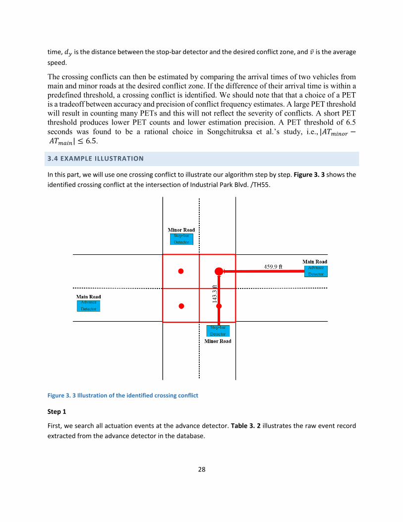
3.4 EXAMPLE ILLUSTRATION
In this part, we will use one crossing conflict to illustrate our algorithm step by step. Figure 3. 3 shows the
identified crossing conflict at the intersection of Industrial Park Blvd. /TH55.
Figure 3. 3 Illustration of the identified crossing conflict
Step 1
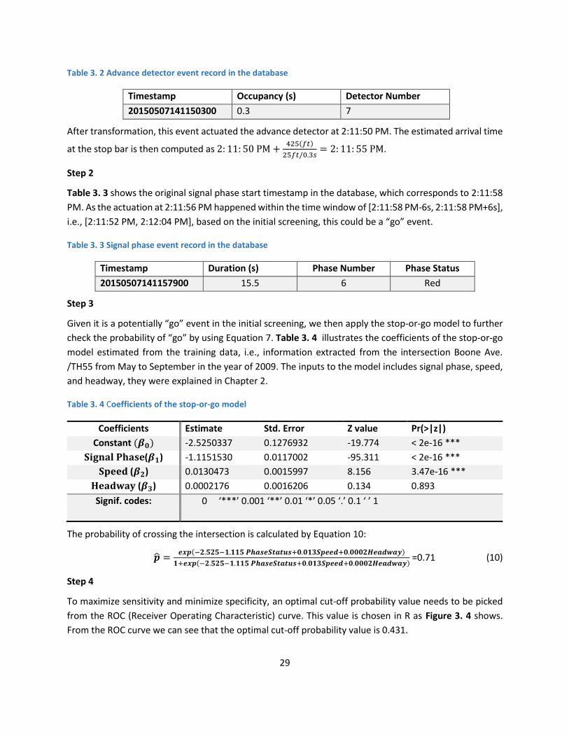
First, we search all actuation events at the advance detector. Table 3. 2 illustrates the raw event record
extracted from the advance detector in the database.
29
Table 3. 2 Advance detector event record in the database
Timestamp Occupancy (s) Detector Number
20150507141150300 0.3 7
After transformation, this event actuated the advance detector at 2:11:50 PM. The estimated arrival time
at the stop bar is then computed as 2: 11: 50 PM +425(𝑓𝑡)
25𝑓𝑡/0.3𝑠= 2: 11: 55 PM.
Step 2
Table 3. 3 shows the original signal phase start timestamp in the database, which corresponds to 2:11:58
PM. As the actuation at 2:11:56 PM happened within the time window of [2:11:58 PM-6s, 2:11:58 PM+6s],
i.e., [2:11:52 PM, 2:12:04 PM], based on the initial screening, this could be a “go” event.
Table 3. 3 Signal phase event record in the database
Timestamp Duration (s) Phase Number Phase Status
20150507141157900 15.5 6 Red
Step 3
Given it is a potentially “go” event in the initial screening, we then apply the stop-or-go model to further
check the probability of “go” by using Equation 7. Table 3. 4 illustrates the coefficients of the stop-or-go
model estimated from the training data, i.e., information extracted from the intersection Boone Ave.
/TH55 from May to September in the year of 2009. The inputs to the model includes signal phase, speed,
and headway, they were explained in Chapter 2.
Table 3. 4 Coefficients of the stop-or-go model
Coefficients Estimate Std. Error Z value Pr(>|z|)
Constant (𝜷𝟎) -2.5250337 0.1276932 -19.774 < 2e-16 ***
𝐒𝐢𝐠𝐧𝐚𝐥 𝐏𝐡𝐚𝐬𝐞(𝜷𝟏) -1.1151530 0.0117002 -95.311 < 2e-16 ***
𝐒𝐩𝐞𝐞𝐝 (𝜷𝟐) 0.0130473 0.0015997 8.156 3.47e-16 ***
𝐇𝐞𝐚𝐝𝐰𝐚𝐲 (𝜷𝟑) 0.0002176 0.0016206 0.134 0.893
Signif. codes: 0 ‘***’ 0.001 ‘**’ 0.01 ‘*’ 0.05 ‘.’ 0.1 ‘ ’ 1
The probability of crossing the intersection is calculated by Equation 10:
�̂� =𝒆𝒙𝒑(−𝟐.𝟓𝟐𝟓−𝟏.𝟏𝟏𝟓 𝑷𝒉𝒂𝒔𝒆𝑺𝒕𝒂𝒕𝒖𝒔+𝟎.𝟎𝟏𝟑𝑺𝒑𝒆𝒆𝒅+𝟎.𝟎𝟎𝟎𝟐𝑯𝒆𝒂𝒅𝒘𝒂𝒚)
𝟏+𝒆𝒙𝒑(−𝟐.𝟓𝟐𝟓−𝟏.𝟏𝟏𝟓 𝑷𝒉𝒂𝒔𝒆𝑺𝒕𝒂𝒕𝒖𝒔+𝟎.𝟎𝟏𝟑𝑺𝒑𝒆𝒆𝒅+𝟎.𝟎𝟎𝟎𝟐𝑯𝒆𝒂𝒅𝒘𝒂𝒚) =0.71 (10)
Step 4
To maximize sensitivity and minimize specificity, an optimal cut-off probability value needs to be picked
from the ROC (Receiver Operating Characteristic) curve. This value is chosen in R as Figure 3. 4 shows.
From the ROC curve we can see that the optimal cut-off probability value is 0.431.

30
Figure 3. 4 ROC (Receiver Operating Characteristic) curve in R
Step 5
Figure 3. 4 illustrated the optimal cutoff threshold which is trained by our training dataset. If the
probability is greater than cutoff threshold, it is considered as a “go” event, otherwise it is a “stop” event.
The estimated “go” probability for this vehicle is 0.71 which is greater than the cutoff threshold 0.431,
thus this event is determined as a “go” event.
Step 6
For this “go” event, the arrival time from the major road at desired conflict zone is calculated by Equation
8 as 𝐴𝑇𝑚𝑎𝑖𝑛 = 2: 11: 50 PM +459.9 (𝑓𝑡)
25𝑓𝑡
0.3
= 2: 11: 56 PM.
Step 7
We need to check if there is a vehicle coming from the minor road and arrive at the desired conflict zone
at the same time. By checking the stop bar detector on the minor road, one actuation record is found
(shown in

31
Table 3. 5). This event actuates the stop-bar detector #14 at 2:11:47 PM with an occupancy of 2.7 second.
Table 3. 5 Stop-bar detector event record in the database
Timestamp Occupancy (s) Detector Number
20150507141147100 2.7 14
Step 8
The arrival time of the vehicle from the minor road at desired conflict zone is calculated by Equation 9 as
𝐴𝑇𝑚𝑖𝑛𝑜𝑟 = 2: 11: 47 PM + 2.7s +143.3 (𝑓𝑡)
25𝑓𝑡2.7𝑠
+51.33ft/s
2
= 2: 11: 55 PM, where 51.33 ft/s is the speed limit on the
minor road.
Step 9
The arrival time of two identified events at the desired conflict zone from the main road and minor road
are 2:11:56 PM and 2:11:55 PM, respectively. The arrival time difference is 1s which is smaller than the
threshold 6.5 s.
Step 10
So we identify it as one crossing conflict. This concludes our algorithm of identifying a crossing conflict.
3.5 CROSSING CONFLICTS SUMMARY
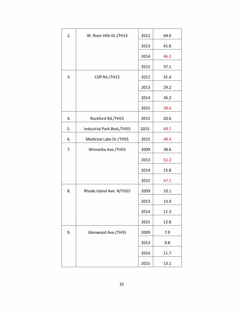
Using the proposed algorithm, we estimated daily crossing conflicts at each intersection for each year.
The result is shown in Table 3. 6. As we can see from the result, the number of daily crossing conflicts
varied across different intersections, mainly from 7.9 to 51.2. The cases highlighted in red were involved
with relatively more crossing conflicts than the others. This could indicate a higher risk of right-angle
collisions at those intersections, and comprehensive safety evaluation may be needed.
Table 3. 6 Estimated crossing conflicts
NO. Intersection name Year Daily
crossing
conflicts
1 Portland Ave./TH13 2012 40.5
2013 16.2
2014 47.5
2015 46.2
32
2. W. River Hills Dr./TH13 2012 44.6
2013 41.8
2014 46.2
2015 37.1
3. Cliff Rd./TH13 2012 31.4
2013 29.2
2014 36.2
2015 39.6
4. Rockford Rd./TH55 2015 20.6
5. Industrial Park Blvd./TH55 2015 49.7
6. Medicine Lake Dr./TH55 2015 48.4
7. Winnetka Ave./TH55 2009 38.6
2013 51.2
2014 15.8
2015 47.1
8. Rhode Island Ave. N/TH55 2009 10.1
2013 13.0
2014 11.3
2015 12.8
9. Glenwood Ave./TH55 2009 7.9
2013 9.8
2014 11.7
2015 13.1
33
CHAPTER 4: RIGHT-ANGLE CRASH MODEL REGRESSION
An important working hypothesis for this research is that the frequency of crossing conflicts at an
intersection could be a reliable indicator of the risk for angle crashes. The idea that non-crash events might
be reliable indicators of crash events dates back to at least to Perkins and Harris (1968), while recently
there has been an emphasis on using traffic conflicts generated in microsimulation programs as predictors
of crash risk (Gettman and Head 2003; Archer and Young 2010). As the Highway Safety Manual (AASHTO
2010) (HSM) documents, however, the most reliable predictor of crash frequency is traffic volume and
one might expect that as traffic volume increases both conflict and crash frequencies would also increase.
A demonstrated correlation between conflict frequency and crash frequency could then be due to conflict
frequency acting as a surrogate for traffic volume rather than being an indicator of crash risk. To test this
hypothesis it is necessary to include measures of both traffic volume and conflict frequency in statistical
models that attempt to predict crash frequency. This chapter describes an initial effort at conducting such
a test. Crash records and average daily traffic data were collected for seven four-legged SMART-SIGNAL
intersections and then the methods described in Chapter 3 were used to compute estimates of the
frequency of crossing conflicts at these intersections. Several versions of a safety performance function
(SPF) similar to that used in the Highway Safety Manual were then evaluated to see if average crossing-
conflict frequency could reliably predict the frequency of angle crashes after controlling for traffic volume.
4.1 DATA PREPARATION
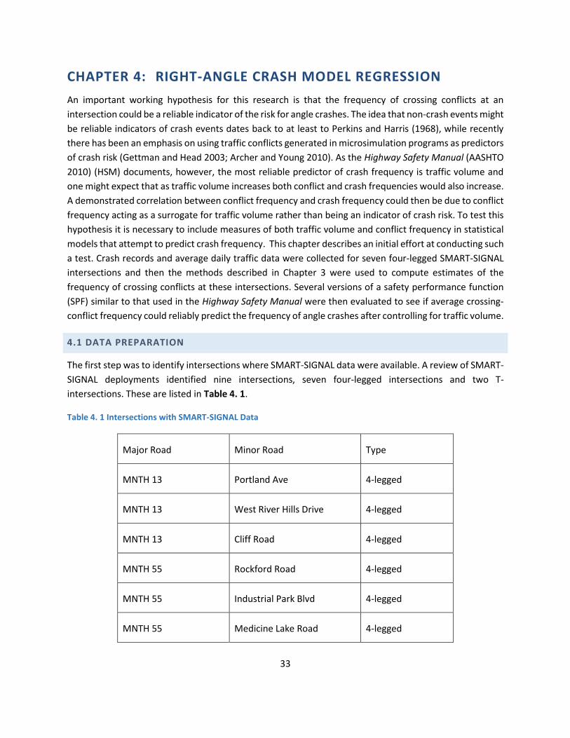
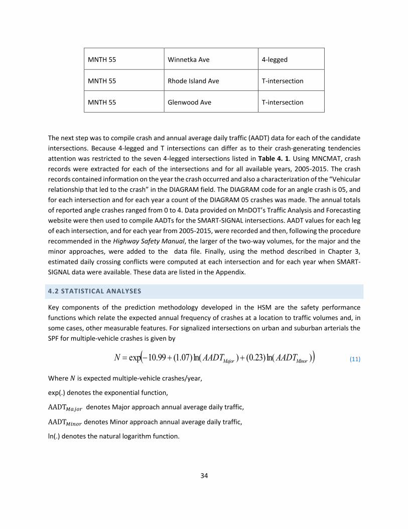
The first step was to identify intersections where SMART-SIGNAL data were available. A review of SMART-
SIGNAL deployments identified nine intersections, seven four-legged intersections and two T-
intersections. These are listed in Table 4. 1.
Table 4. 1 Intersections with SMART-SIGNAL Data
Major Road Minor Road Type
MNTH 13 Portland Ave 4-legged
MNTH 13 West River Hills Drive 4-legged
MNTH 13 Cliff Road 4-legged
MNTH 55 Rockford Road 4-legged
MNTH 55 Industrial Park Blvd 4-legged
MNTH 55 Medicine Lake Road 4-legged
34
MNTH 55 Winnetka Ave 4-legged
MNTH 55 Rhode Island Ave T-intersection
MNTH 55 Glenwood Ave T-intersection
The next step was to compile crash and annual average daily traffic (AADT) data for each of the candidate
intersections. Because 4-legged and T intersections can differ as to their crash-generating tendencies
attention was restricted to the seven 4-legged intersections listed in Table 4. 1. Using MNCMAT, crash
records were extracted for each of the intersections and for all available years, 2005-2015. The crash
records contained information on the year the crash occurred and also a characterization of the “Vehicular
relationship that led to the crash” in the DIAGRAM field. The DIAGRAM code for an angle crash is 05, and
for each intersection and for each year a count of the DIAGRAM 05 crashes was made. The annual totals
of reported angle crashes ranged from 0 to 4. Data provided on MnDOT’s Traffic Analysis and Forecasting
website were then used to compile AADTs for the SMART-SIGNAL intersections. AADT values for each leg
of each intersection, and for each year from 2005-2015, were recorded and then, following the procedure
recommended in the Highway Safety Manual, the larger of the two-way volumes, for the major and the
minor approaches, were added to the data file. Finally, using the method described in Chapter 3,
estimated daily crossing conflicts were computed at each intersection and for each year when SMART-
SIGNAL data were available. These data are listed in the Appendix.
4.2 STATISTICAL ANALYSES
Key components of the prediction methodology developed in the HSM are the safety performance
functions which relate the expected annual frequency of crashes at a location to traffic volumes and, in
some cases, other measurable features. For signalized intersections on urban and suburban arterials the
SPF for multiple-vehicle crashes is given by
)ln()23.0()ln()07.1(99.10exp MinorMajor AADTAADTN (11)
Where 𝑁 is expected multiple-vehicle crashes/year,
exp(.) denotes the exponential function,
AADT𝑀𝑎𝑗𝑜𝑟 denotes Major approach annual average daily traffic,
AADT𝑀𝑖𝑛𝑜𝑟 denotes Minor approach annual average daily traffic,
ln(.) denotes the natural logarithm function.
35
For example, at an intersection where the AADT on both the Major and Minor approaches was 1.0
vehicles/day, the expected crash frequency would be exp(-10.99)=0.000017 crashes/year. A 1% increase
in Major approach AADT leads to a 1.07% increase in predicted crash frequency while a 1% increase in
Minor approach AADT leads to a 0.23% increase in predicted crash frequency. At an intersection with a
Major AADT of 10,000 vehicles/day and a Minor AADT of 2000 vehicles/day the predicted crash frequency
is
yearcrashes /85.1)2000ln()23.0()10000ln()07.1(99.10exp
The HSM also notes that typically about 25% of multi-vehicle crashes are angle crashes.
As a first step it was decided to fit a similar SPF for angle crashes at the seven four-legged SMART-SIGNAL
intersections using all available crash and AADT data. Annual crash counts were treated as independent
Poisson outcomes with expected values following the SPF
)ln()()ln()(exp 321 MinorMajor AADTAADTN (12)
As in the above example the coefficient 1 in equation (12) is related to the expected crash frequency
when traffic volumes are minimal while the coefficients 2 and 3 give the predicted increases in crash
frequency associated with 1% increases in Major and Minor approach traffic volumes. A value 2=0 means
that changes in Major approach AADT have no effect on predicted crash frequency while a value of 3=0
means Minor approach AADT has no effect on crash frequency.
Maximum likelihood estimates of the coefficients β1, β2, and β3 appearing in equation (12) were computed
using Mathcad’s (Maxfield 2009) nonlinear equation solver, while statistical inference was based on
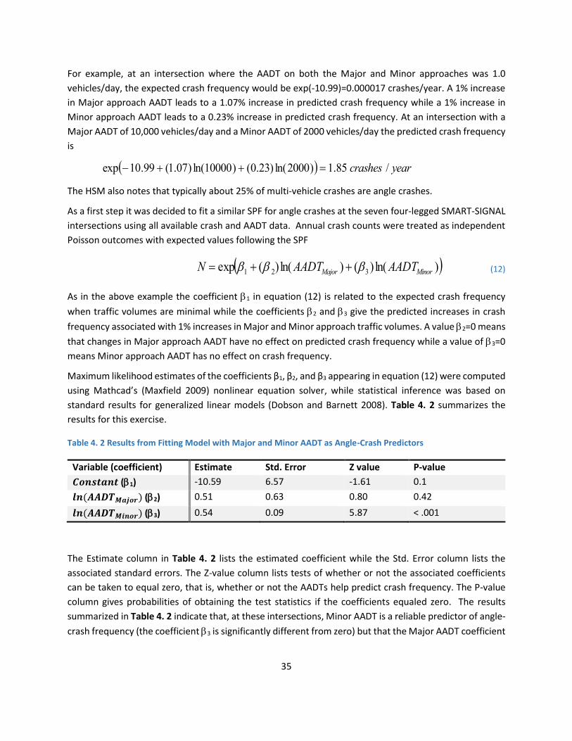
standard results for generalized linear models (Dobson and Barnett 2008). Table 4. 2 summarizes the
results for this exercise.
Table 4. 2 Results from Fitting Model with Major and Minor AADT as Angle-Crash Predictors
Variable (coefficient) Estimate Std. Error Z value P-value
𝑪𝒐𝒏𝒔𝒕𝒂𝒏𝒕 (1) -10.59 6.57 -1.61 0.1
𝒍𝒏(𝑨𝑨𝑫𝑻𝑴𝒂𝒋𝒐𝒓) (2) 0.51 0.63 0.80 0.42
𝒍𝒏(𝑨𝑨𝑫𝑻𝑴𝒊𝒏𝒐𝒓) (3) 0.54 0.09 5.87 < .001
The Estimate column in Table 4. 2 lists the estimated coefficient while the Std. Error column lists the
associated standard errors. The Z-value column lists tests of whether or not the associated coefficients
can be taken to equal zero, that is, whether or not the AADTs help predict crash frequency. The P-value
column gives probabilities of obtaining the test statistics if the coefficients equaled zero. The results
summarized in Table 4. 2 indicate that, at these intersections, Minor AADT is a reliable predictor of angle-
crash frequency (the coefficient 3 is significantly different from zero) but that the Major AADT coefficient
36
2 is not significantly different from zero. That is, knowledge of Major AADT does not help predict angle-
crash frequency. This finding is confirmed by using the likelihood-ratio test to compare equation (12) to a
simpler model having only the constant term and Minor AADT as predictors. The computed Chi-squared
statistic was 0.384, with one degree-of-freedom and a p-value of 0.464, indicating that an SPF without
Major AADT and one with Major AADT provided essentially equivalent descriptions of how the crash
frequencies varied. The failure of Major AADT to help predict crash frequency is probably due the fact
that the intersections were neighbors along two trunk highways so that the Major approach AADTs
showed little site-to-site variation.
The next set of analyses looked to see if adding a measure of crossing conflicts improved the ability to
predict angle crashes. Since SMART-SIGNAL data were available for at most four years these analyses were
based on a limited crash experience (11 crashes total) and so should be regarded as preliminary.
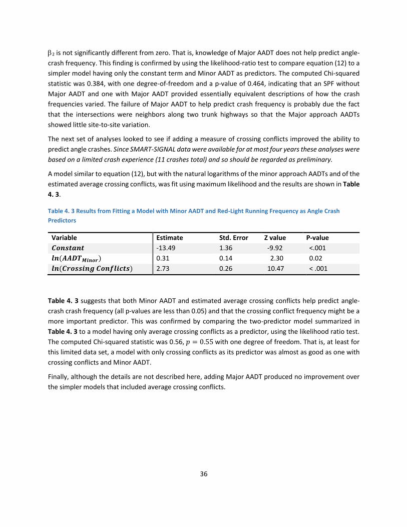
A model similar to equation (12), but with the natural logarithms of the minor approach AADTs and of the
estimated average crossing conflicts, was fit using maximum likelihood and the results are shown in Table
4. 3.
Table 4. 3 Results from Fitting a Model with Minor AADT and Red-Light Running Frequency as Angle Crash
Predictors
Variable Estimate Std. Error Z value P-value
𝑪𝒐𝒏𝒔𝒕𝒂𝒏𝒕 -13.49 1.36 -9.92 <.001
𝒍𝒏(𝑨𝑨𝑫𝑻𝑴𝒊𝒏𝒐𝒓) 0.31 0.14 2.30 0.02
𝒍𝒏(𝑪𝒓𝒐𝒔𝒔𝒊𝒏𝒈 𝑪𝒐𝒏𝒇𝒍𝒊𝒄𝒕𝒔) 2.73 0.26 10.47 < .001
Table 4. 3 suggests that both Minor AADT and estimated average crossing conflicts help predict angle-
crash crash frequency (all p-values are less than 0.05) and that the crossing conflict frequency might be a
more important predictor. This was confirmed by comparing the two-predictor model summarized in
Table 4. 3 to a model having only average crossing conflicts as a predictor, using the likelihood ratio test.
The computed Chi-squared statistic was 0.56, 𝑝 = 0.55 with one degree of freedom. That is, at least for
this limited data set, a model with only crossing conflicts as its predictor was almost as good as one with
crossing conflicts and Minor AADT.
Finally, although the details are not described here, adding Major AADT produced no improvement over
the simpler models that included average crossing conflicts.
37
CHAPTER 5: CONCLUSION
In this project, we developed two methodologies for intersection safety evaluation using high-resolution
traffic signal data collected from the SMART-Signal system: red-light running (RLR) for those with stop-bar
and entrance detectors; and crossing conflicts for those with only advance detectors, based on our work
on stop-or-go prediction modeling.
Then we tested whether adding a measure of red-light running to a more standard model containing
AADTs could improve the ability to predict angle crashes at signalized intersections. Although any
conclusion should be regarded as preliminary, due to the limited data available, for these data, it appears
that the crossing conflict measures are superior to either major approach AADT or minor approach AADT
as a predictor of angle-crash frequency.
In the future, the work proposed in this project may be extended in two directions. First, we may improve
the prediction accuracy of the developed model when more data collected from the SMART-SIGNAL
system becomes available. Second, video cameras can be installed at intersections to validate our
proposed methodologies.

38
REFERENCES
Abbas, M., Machiani, S. G., Garvey, P. M., Farkas, A., and Lord-Attivor, R. (2014). Modeling the
Dynamics of Driver's Dilemma Zone Perception Using Machine Learning Methods for Safer
Intersection Control (No. MAUTC-2012-04).
Abdel-Aty, M., Lee, C., Wang, X., Nawathe, P., Keller, J., Kowdla, S., and Prasad, H. (2006). Identification
of Intersections' Crash Profiles/Patterns.
Amundson, F.H., and Hyden, C., (1977). Proceedings of the First Workshop on Traffic Conflict,
Institution of Transport Economics, Lind Institute of Technology, Oslo, Norway.
Archer, J., (2005). Indicators for traffic safety assessment and prediction and their application
in micro-simulation modelling: a study of urban and suburban inter-sections. In: Doctoral
Dissertation. Department of Infrastructure, Division for Transport and Logistic (TOL), Centre for
Transport Research, Royal Institute of Technology, Stockholm, Sweden.
AASHTO, Highway Safety Manual, American Association of State Highway and Transportation
Officials, (2010).
Archer, J., and Young, W. (2010, January). A traffic microsimulation approach to estimate safety at
unsignalised intersections. In Transportation Research Board Annual Meeting, 89th, 2010, Washington,
DC, USA (No. 10-0683).
Bonneson, J., and Son, H. (2003). Prediction of expected red-light-running frequency at urban
intersections. Transportation Research Record: Journal of the Transportation Research Board, (1830),
38-47.
Chatterjee, I., and Davis, G. A. (2011). Can High-Resolution Detector and Signal Data Support
Intersection Crash Identification and Reconstruction? In 3rd International Conference on Road Safety
and Simulation.
Dobson, A., and Barnett, A., An Introduction to Generalized Linear Models, third edition, CRC
Press, 2008.
Elmitiny, N., Yan, X., Radwan, E., Russo, C., and Nashar, D. (2010). Classification analysis of driver's
stop/go decision and red-light running violation. Accident Analysis and Prevention, 42(1), 101-111.
Gates, T., Noyce, D., Laracuente, L., and Nordheim, E. (2007). Analysis of driver behavior in dilemma
zones at signalized intersections. Transportation Research Record: Journal of the Transportation
Research Board, (2030), 29-39.
39
Gettman, D., and Head, L. (2003). Surrogate safety measures from traffic simulation
models. Transportation Research Record: Journal of the Transportation Research Board, (1840), 104-
115.
Liu, Y., Chang, G. L., Tao, R., Hicks, T., and Tabacek, E. (2007). Empirical observations of dynamic
dilemma zones at signalized intersections. Transportation Research Record: Journal of the
Transportation Research Board, (2035), 122-133.
Liu, H. X., Wu, X., Ma, W., and Hu, H. (2009). Real-time queue length estimation for congested signalized
intersections. Transportation research part C: emerging technologies, 17(4), 412-427.
Maxfield, B. (2009). Essential Mathcad for Engineering, Science, and Math W/CD. Academic Press.
Mitra, S., Chin, H. C., and Quddus, M. (2002). Study of intersection accidents by maneuver
type. Transportation Research Record: Journal of the Transportation Research Board, (1784), 43-50.
Perkins, S. R., and Harris, J. L. (1968). Traffic conflict characteristics-accident potential at intersections.
Highway Research Record, (225).
Poch, M., and Mannering, F. (1996). Negative binomial analysis of intersection-accident
frequencies. Journal of transportation engineering, 122(2), 105-113.
Porter, B. E., and Berry, T. D. (2001). A nationwide survey of self-reported red light running: measuring
prevalence, predictors, and perceived consequences. Accident Analysis and Prevention, 33(6), 735-741.
Porter, B. E., and England, K. J. (2000). Predicting red-light running behavior: a traffic safety study in
three urban settings. Journal of Safety Research, 31(1), 1-8.
Papaioannou, P. (2007). Driver behaviour, dilemma zone and safety effects at urban signalised
intersections in Greece. Accident Analysis and Prevention, 39(1), 147-158.
Perkins, S. R., and Harris, J. L. (1968). Traffic conflict characteristics-accident potential at
intersections. Highway Research Record, (225).
Rakha, H., and El-Shawarby, I., and Setti, J.R., (2007). Characterizing driver behavior on
signalized intersection approaches at the onset of a yellow-phase trigger. IEEE Transactions on
Intelligent Transportation Systems, 8(4): 630-640.
Retting, R., Williams, A., and Greene, M. (1998). Red-light running and sensible countermeasures:
Summary of research findings. Transportation Research Record: Journal of the Transportation Research
Board, (1640), 23-26.
Sharma, A., Bullock, D. and Peeta, S., (2011). Estimating dilemma zone hazard function at high-
speed isolated intersection. Transportation research part C. 19 (3): 400 —412

40
Songchitruksa, P., and Tarko, A. (2006). Practical method for estimating frequency of right-angle
collisions at traffic signals. Transportation Research Record: Journal of the Transportation Research
Board, (1953), 89-97.
Sayed, T., Brown, G., and Navin, F. (1994). Simulation of traffic conflicts at unsignalized intersections
with TSC-Sim. Accident Analysis and Prevention, 26(5), 593-607.
Songchitruksa, P., and Tarko, A. (2006). Practical method for estimating frequency of right-angle
collisions at traffic signals. Transportation Research Record: Journal of the Transportation Research
Board, (1953), 89-97.
Wu, X., Vall, N., Liu, H., Cheng, W., and Jia, X. (2013). Analysis of drivers' stop-or-run behavior at
signalized intersections with high-resolution traffic and signal event data. Transportation Research
Record: Journal of the Transportation Research Board, (2365), 99-108.
Yang, C. D., and Najm, W. G. (2007). Examining driver behavior using data gathered from red light photo
enforcement cameras. Journal of safety research, 38(3), 311-321.
Zhang, L., Zhou, K., Zhang, W. B., and Misener, J. (2009). Prediction of red light running based on
statistics of discrete point sensors. Transportation Research Record: Journal of the Transportation
Research Board, (2128), 132-142.

APPENDIX A: DATA USED IN CRASH PREDICTION ANALYSES

A-1
Intersection Year Angle
Crashes
Minor
AADT
Major
AADT
Average Crossing
Conflicts
Portland Ave./TH13 2005 0 3000 31500 NA
2006 1 3000 29500 NA
2007 0 3200 29500 NA
2008 1 3200 29000 NA
2009 0 3200 29000 NA
2010 1 3400 30000 NA
2011 0 3400 30000 NA
2012 0 3400 30500 40.5
2013 0 3400 30500 16.15
2014 2 3250 30500 47.47
2015 0 3250 29500 46.2
W. River Hills Dr./TH13 2005 1 10800 28000 NA
2006 1 10500 28500 NA
2007 1 9800 28500 NA
2008 0 9800 28500 NA
2009 0 9800 28500 NA
2010 0 9800 28000 NA
2011 1 9500 28000 NA
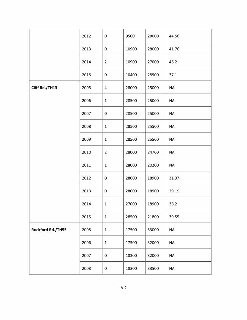
A-2
2012 0 9500 28000 44.56
2013 0 10900 28000 41.76
2014 2 10900 27000 46.2
2015 0 10400 28500 37.1
Cliff Rd./TH13 2005 4 28000 25000 NA
2006 1 28500 25000 NA
2007 0 28500 25000 NA
2008 1 28500 25500 NA
2009 1 28500 25500 NA
2010 2 28000 24700 NA
2011 1 28000 20200 NA
2012 0 28000 18900 31.37
2013 0 28000 18900 29.19
2014 1 27000 18900 36.2
2015 1 28500 21800 39.55
Rockford Rd./TH55 2005 1 17500 33000 NA
2006 1 17500 32000 NA
2007 0 18300 32000 NA
2008 0 18300 33500 NA
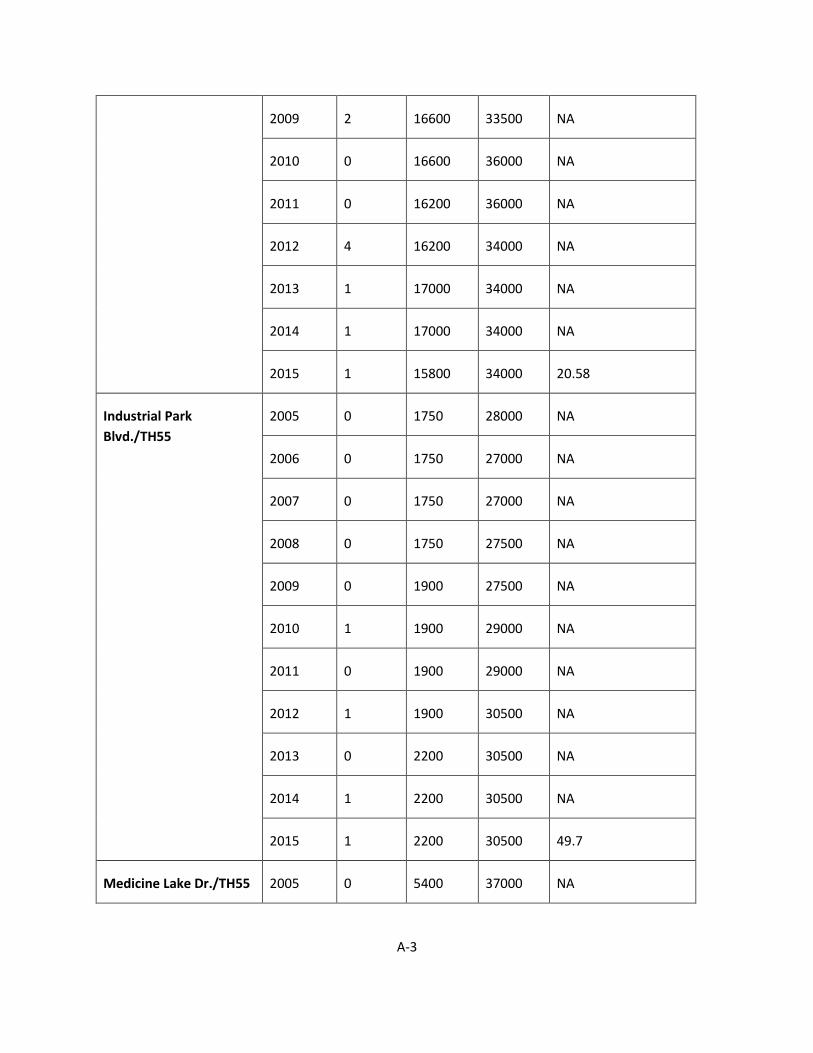
A-3
2009 2 16600 33500 NA
2010 0 16600 36000 NA
2011 0 16200 36000 NA
2012 4 16200 34000 NA
2013 1 17000 34000 NA
2014 1 17000 34000 NA
2015 1 15800 34000 20.58
Industrial Park
Blvd./TH55
2005 0 1750 28000 NA
2006 0 1750 27000 NA
2007 0 1750 27000 NA
2008 0 1750 27500 NA
2009 0 1900 27500 NA
2010 1 1900 29000 NA
2011 0 1900 29000 NA
2012 1 1900 30500 NA
2013 0 2200 30500 NA
2014 1 2200 30500 NA
2015 1 2200 30500 49.7
Medicine Lake Dr./TH55 2005 0 5400 37000 NA
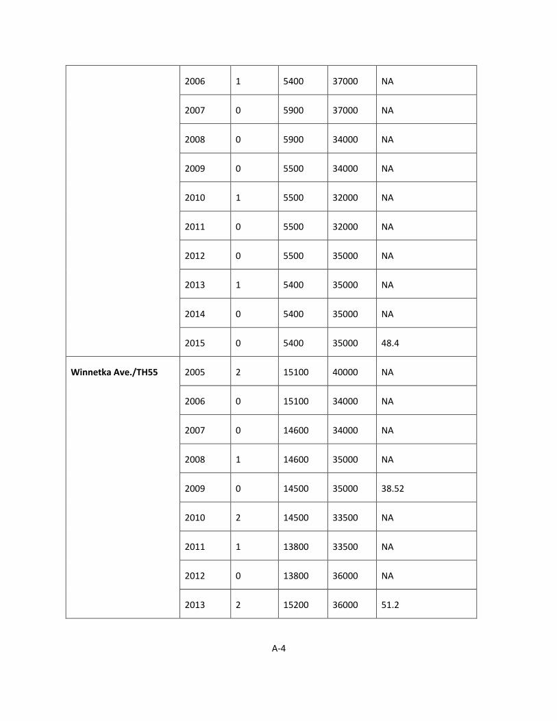
A-4
2006 1 5400 37000 NA
2007 0 5900 37000 NA
2008 0 5900 34000 NA
2009 0 5500 34000 NA
2010 1 5500 32000 NA
2011 0 5500 32000 NA
2012 0 5500 35000 NA
2013 1 5400 35000 NA
2014 0 5400 35000 NA
2015 0 5400 35000 48.4
Winnetka Ave./TH55 2005 2 15100 40000 NA
2006 0 15100 34000 NA
2007 0 14600 34000 NA
2008 1 14600 35000 NA
2009 0 14500 35000 38.52
2010 2 14500 33500 NA
2011 1 13800 33500 NA
2012 0 13800 36000 NA
2013 2 15200 36000 51.2

A-5
2014 0 15200 36000 15.8
2015 1 15800 36000 47.1