estimation of critical gap using maximum likelihood method
TRANSCRIPT

International Journal of Transportation Engineering and Technology 2021; 7(2): 48-59
http://www.sciencepublishinggroup.com/j/ijtet
doi: 10.11648/j.ijtet.20210702.12
ISSN: 2575-1743 (Print); ISSN: 2575-1751 (Online)
Estimation of Critical Gap Using Maximum Likelihood Method at Unsignalized Intersection: A Case Study in Adama City, Ethiopia
Fikedu Rage Faye
Department of Civil Engineering, Mettu University, Mettu, Ethiopia
Email address:
To cite this article: Fikedu Rage Faye. Estimation of Critical Gap Using Maximum Likelihood Method at Unsignalized Intersection: A Case Study in Adama
City, Ethiopia. International Journal of Transportation Engineering and Technology. Vol. 7, No. 2, 2021, pp. 48-59.
doi: 10.11648/j.ijtet.20210702.12
Received: May 29, 2021; Accepted: July 8, 2021; Published: July 15, 2021
Abstract: Studying Critical gap and headway distribution has vital role in reduction of traffic problems. Critical gap and its
distribution are traffic characteristics that are used in determination of capacity, delay and level of service at unsignalized
intersection. Many study has been done on critical gap in developed countries under homogeneous traffic and road conditions.
This study is aimed to insight available headway distribution and critical gap of driver in urban intersection under
heterogeneous traffic condition and weak lane discipline in developing country like Ethiopia. In this paper three unsignalized
intersection in Adama city has been selected on the basis of traffic volume and importance of the intersection. The primary
data that were used for this study were traffic volume, available headways, waiting time, geometry of road. By using digital
Camera, videos data were recorded; later quantitative data were extracted from videos. Two Statistical Packages that were used
in analysis of this study. Statistical Package for Social Science Statistic 20 was used to fit best distribution model of headway.
Kolmogorov Smirnov and Anderson Darling testing techniques were conducted to check validity of model for headways in
different flow ranges. From hypothesized distributions, exponential, gamma, lognormal and normal distributions were selected
for different intersection. It has been indicated that, for higher flow rate lognormal distribution model is best fit in estimating
cumulative density function of headway. Critical gaps of drivers for three selected intersections were also computed by using
maximum likelihood method. Through Comparison of estimated values indicates that, Franko intersection has highest critical
gap of 5.17sec.
Keywords: Headway Distribution, Maneuver Type Maximum Likelihood, Waiting Time
1. Introduction and Literature Review
1.1. Introduction
Average follow-up headway and average critical headway
are two key parameters in the new roundabout capacity model
presented in the R. Morris, M. [14]. Study included statistical
methodology for the estimation of the critical gap, and
demonstrates its application through field measurements. It is
assumed that the critical gap has a lognormal distribution
among the driver population with a mean value that is a
function of a number of explanatory variables. Based on these
assumptions the critical gap and its distribution estimated
using maximum likelihood. A case study in a dual lane
roundabout in Stockholm is used to illustrate the proposed
methodology using video and other data recording techniques.
The results showed that the critical gap depends, among
factors, on the target lane (near or far), the type of the vehicle
and driver age [6]. Critical Gap for merging and crossing,
factors that influences gap acceptances and waiting time to
accept gaps were undermined in many studies in Ethiopia. So
that the researcher is initiated to provide his own role by filling
shortcoming of previous study concerning accessing available
headway distribution and critical gap for drivers who are
merging or crossing major road from minor road.
1.2. Need of Present Study
In ideal world where traffic flow is managed properly

International Journal of Transportation Engineering and Technology 2021; 7(2): 48-59 49
through traffic management system, where driver is design
driver and other road users who can easily understand
regulation of traffic rule, studying traffic characteristics like
headway distribution, and critical headway, congestion, delay
and level of service of intersection is not such mandatory.
But since we live in real world transportation system
problems and difficulties faces road users and policy makers
from time to time. Despite we can minimize in systematic
manner, we cannot avoid it. In Ethiopia there is a rapid
increase in the number of the vehicles and their varieties
which creates a headache for the transportation professionals
and policy makers. As such type of traffic flow consists of a
wide range of complex activities, embracing vehicle arrivals,
speed of travel, lane discipline, un- necessary overtaking,
mixed traffic flow and crossing logic, gap acceptance,
waiting time, available headway, acceleration and
deceleration. So that the researcher is initiated to put his own
role by doing scientific research on headway distribution and
available critical gaps which gives some understanding for
road users (drivers, passengers and pedestrians) and
professionals.
1.3. Objective of Study
The general objective of this study is to investigate
distribution patterns of available headways to be accepted
and rejected and also evaluate critical gaps that are available
for the drivers in study in urban area.
1.4. Review Literature
A number of studies has been conducted on headways and
critical gaps for the drivers. In this paper some studies which
are more closely with study has been included. Time
headway distribution is helpful to insight the disaggregate
flow of traffic which is very important in capacity and level
of service determination [10]. Video graphic data were
collected for four road section in Assam city, later data were
extracted and analyzed. The distribution of headways for
different flow rates by increment of 200PCU/hr. also shown
by Maurya, A. [13]. It has been shown Log Pearson-3 is best
fit distribution for low flow rate up to 600PCU/hr. and
Inverse Gaussian distribution for high flow rate greater than
800PCU/hr. Another study that was done in Oregon state
university by Abd-Elaziz, A., & Abd-Elwahab, S. [1], shows
that non parametric approach to fit best distribution for
headway. Using K-S test hypothesized distribution was
rejected or accepted at 95 confidence interval. In this study
headway distribution was made vehicle to vehicle interaction
with their categories. Gaussian Kernel curve was developed
and analyzed for selected interaction. The same study has
been conducted in west Bengal city to show the headway
distribution model by Abhishek, O., & Marko A. A. Boon,
R.-Q. [2] In India. Data were collected to observe time
headways on a National Highway (two-lane highway) in the
north-east India, popularly known as the Assam-Agartala
road. A highway section of about 20 km length, close to the
capital city. Data were captured ideographically. Based on
collected data. Lognormal, Person 3P and Log logistics were
selected model for different pair of traffic in category wise.
The method of Raff is based on macroscopic model and it
is the earliest method for estimating the critical gap which is
used in many countries because of its simplicity. This method
involves the empirical distribution functions of accepted gaps
Fa(t) and rejected gaps Fr(t). When the sum of cumulative
probabilities of accepted gaps and rejected gaps is to equal 1
then a gap of length tis equal to critical gap (tc). It means the
number of rejected gaps larger than critical gap is equal to the
number of accepted gaps smaller than critical gap. As Amin,
H. J. [5] Empirical distribution accepted gap has been given
by the following equation.
����� = 1 − ���� Where,
Fa: empirical distribution of accepted gap
Fr: empirical distribution of rejected gap
Dutta, M. M. [10] Used maximum likely hood method for
estimating critical gaps was based on the Maximum
likelihood method (MLM). The MLM is based on the
assumption that minor stream drivers behave consistently. It
means that each driver will reject every gap smaller than his
critical gap and will accept the first gap larger than the
critical gap. Under this assumption, the distribution of the
critical gaps lies between distributions of largest rejected and
accepted gaps. The parameters of distribution function of the
critical gaps, the mean (µ) and variance (σ2) are obtained by
maximizing the likelihood function by Akhilesh, M. K [3].
=�[��� �
��� − �� �]
Where, L: maximum likelihood function, ai: logarithm of
the accepted gap of driver i,
ri: logarithm of the maximum rejected gap of driver
F(ai) and F(ri): cumulative distribution functions for the
normal distribution.
Al-Obaed [4] Estimated critical gaps by nine important
methods Raff, Wu, Logit, Ashworth, Lag, and Harder,
Acceptance curve, clearing behavior, Green shield for
turning left and turning right maneuver type. Amin, H. J.
[5] Computed critical gap by three most common
techniques for 5 study location in Italy city. These
techniques were maximum likely hood, Raff method and
median method. [6] Used Logit model to compute critical
gap of driver at unsignalized intersection. The same study
has been conducted in Minnesota university by Arvind. M
[7] in Minnesota City for 8 intersection. Report shows that
three techniques has been used to estimate critical gaps for
driver for left turning and right turning traffic. These
techniques used were maximum likelihood, raff method
and median method. Another study in America was
conducted by Akhilesh and M. K [3] also uses maximum
likelihood to estimate driver critical gap to accept the
available headway.

50 Fikedu Rage Faye: Estimation of Critical Gap Using Maximum Likelihood Method at Unsignalized
Intersection: A Case Study in Adama City, Ethiopia
2. Materials and Methods
2.1. Location of Study
The study area is Adama city which is located in Ethiopia,
Oromia national regional state, east Showa zone at a distance
of 99 km from the capital city Addis Ababa. Adama city is
located at 8.54° N and 39.27° E. It is one of the reform cities
in the region and consists of 14 urban and 4 rural Kebeles.
With an area of 29.86square kilometers and a population
density of 7,374.82/ km2, all are urban inhabitants. Based on
2007 census, a total of 60,174 households were counted in
the city, which results in an average of 3.66 persons to a
household, and 59,431 housing units. According to INSA
131,000 parcel are there currently in Adama city
administration. Here Study area has been shown on figure 1.
2.2. Traffic Condition
Adama city (Nazareth) is one of the cities which have
higher traffic characterized by being the junction of four
main transport routes that connect to different parts of the
country to Addis Ababa, to Djibouti/ Harar, to Wonji, to
Arsi-Bale, Shashamene-Hawassa. The city has a big and
strategic vision of being/to become a center of
trade/commerce and conference for the whole Ethiopia, and
the Oromia regional state in particular. Fortunately, the city is
located at the center and nearby distances of natural tourist
attractions, especially natural and historical tourist centers in
Oromia regional state, South nation nationalities and people’s
regional state, including Afar and Harar regional state. In
Adama city various road transportation like Carts, Bajaj, and
Other vehicular and non-vehicular mode are visible. Road
network in this city has both national and regional
importance.
Figure 1. Map of Study Area.
2.3. Data Collection and Survey Method
Collection and analysis of data were based up on selected
intersection of Adama city. Three unsignalized intersection
that were selected for this study were; Franko Intersection,
Tikur Abay intersection and Wonji Mazoria intersection
2.3.1. Headway
Headway is defined as the time interval between two
successive vehicles as they pass a point along the lane, also
measured between common reference points on the vehicles.
The average headway in lane directly related the rate of flow [8].

International Journal of Transportation Engineering and Technology 2021; 7(2): 48-59 51
� = 3600��
Where v=Rate of flow, Veh/h/ln
Ha=Headway in second.
There are various methods to collect the time headway of
the vehicle moving on a street, Manual Method, Video-
graphic techniques, Lever Mechanism, By Tape Recorder,
Multiple Tap recorder. In order Improve accuracy, the data
were collected by video graphic method by using digital
camera. Video was recorded for 12 hrs. Starts from 7:00 am
to 7:00 pm. Later data were extracted by using stop watch.
The vehicle arrivals were noted down by the observers. The
difference of time arrivals between the two successive
vehicles then gave the time headway between the two
vehicles. The time gap also determined in the same way but it
is taken only the time in which the first vehicle passing the
reference and the time of arrival of the following vehicle.
The stop watch was used to determine the time difference
between the two incidents. Data collection was done vehicle
categorize wise. Table 1 declares that Vehicle to vehicle
interaction and abbreviation used.
Table 1. Vehicles Category with Assigned Symbols.
Vehicle Category Abbreviated Back Vehicle Front Vehicle Assigned As
Bajaj B Bajaj Cart B-Ca
Bus (Coach) Bu Bus (Coach) Small Bus Bu-SB
Car C Car Truck C-T
Pickup (4 Wheel Drive) P Pickup (4 Wheel Drive) Truck-Trailer P-TT
Cart Ca Cart Two Wheeler Ca-TW
Small Bus SB Small Bus Bajaj SB-B
Truck T Truck Bus (Coach) T-Bu
Truck-Trailer TT Truck-Trailer Car TT-C
Two Wheeler TW Two Wheeler Pickup (4 Wheel Drive) TW-P
2.3.2. Road Geometry Measuring
The road geometry of major and minor road has great influence on traffic flow characteristics like headway, speed, volume,
delay on Intersection and gap accepting condition
Table 2. Geometric Characteristic in meters.
Intersection Name Major Road Minor Road
Road Width Shoulder Width Road Width Shoulder Width
Franko 12.4 1.2 11.6 1.2
Tikur Abay 9.6 0.80 9.4 0.80
Wonji Mazoria 12.0 1.00 9.6 1.00
2.4. Data Processing and Analysis
Statistical Packages that were used in analysis of this study
were SPSS Statistic 20 and Minitab. SPSS Statistic 20 was
used fit best distribution model of headway and K-S
technique was used for validation of model for headways in
different flow ranges. Critical gap estimation and
determining of headway distribution pattern of available gaps
are aim of this study. After collection of headway, accepted
and rejected gap, grouping of headways based on flow rate
and vehicle to vehicle interaction. Estimation of best fit
distribution and
Critical gap for left turning and right turning traffic using
maximum likelihood method. Later validation of model was
made by K-S and AD techniques. Figure 3 shows method of
data analysis for this study.
3. Result and Discussion
This section includes investigation and detail of study,
quantitative data analysis, development of models testing
fitness (validation) was done for evaluation of critical gap for
selected unsignalized intersection in Adama city.
3.1. Headway Analysis
The basic statistical properties headway on major road of
selected intersections’ range, minimum, maximum, mean and
standard deviation was shown in Table 3. It is observed that
average headways in seconds on major road are 5.58sec,
8.42sec and 7.51sec for Franko, Tikur Abay and Wonji
Mazoria intersection respectively. These numbers indicated
the traffic at Franko intersection is densely populated on the
road and Wonji Mazoria has less density compared to other
intersection
Table 3. Statistical Properties of Headway per 15’ in seconds.
Intersection’s
Name Range Minimum Maximum
Mean
Statistic St.Dev
Franko 37.40 .20 37.60 5.5803 .22495
Tikur Abay 40.00 .00 40.00 8.4297 .29367
W/Mazoria 39.00 .30 39.30 7.5156 .28088
Variation of basic statistical properties of headways for
different flow rate ranges for three intersections has been
shown on Table 4. Small headways indicate that traffic are
moving in low speed (high flow rate). For three intersections
the median values are less the average values of headways

52 Fikedu Rage Faye: Estimation of Critical Gap Using Maximum Likelihood Method at Unsignalized
Intersection: A Case Study in Adama City, Ethiopia
mean that 50% of vehicles are moving in time headways less
than average values. Consider variance of headways for
different flow rates greater variability is observed at low flow
rate. It indicates that if flow of traffic is low (nearly
congested) drivers selects the possible paths to go forward
inconsistently. So that high fluctuation of headway is
observed at low flow rate (600-800PCU) at Franko
intersection.
Table 4. Statistical properties of Headway on major road PCU classes in seconds.
Flow Range (PCU/Hr.) Intersection Minimum- Maximum Mean Median St. Dev
600-800
Franko - - - - -
T/Abay .66 38.30 12.6887 10.7000 9.33080
W/Mazoria - - - - -
800-1000
Franko - - - - -
T/Abay .20 39.13 9.7087 6.6500 8.51863
W/Mazoria 1.11 39.89 16.5681 15.6000 9.23618
1000-1200
Franko .60 26.09 10.7256 10.3900 7.46652
T/Abay .09 38.75 9.0592 5.7700 8.27516
W/Mazoria .71 36.13 12.0180 9.6000 9.13720
1200-1400
Franko .35 37.60 8.7030 4.6050 8.94724
T/Abay .20 40.00 8.2329 4.7300 8.16933
W/Mazoria .29 111.46 10.5368 9.6000 12.13952
1400-1600
Franko .23 31.43 5.8145 3.7600 5.58164
T/Abay .00 38.81 6.5972 4.1000 6.62220
W/Mazoria .20 38.82 8.1054 5.5100 8.04629
1600-1800
Franko .20 25.00 3.1384 2.5000 2.56290
T/Abay .20 31.80 5.7754 3.7700 5.56421
W/Mazoria .18 39.01 6.3713 4.6950 6.53948
1800-2000
Franko .27 17.50 3.1636 1.8000 3.51868
T/Abay - - - - -
W/Mazoria .78 17.84 3.5779 4.0150 2.63487
2000-2200
Franko .40 2.70 1.3749 1.1800 .81730
T/Abay - - - - -
W/Mazoria .57 6.44 3.0069 2.8000 1.55189
Type of vehicle to vehicle interaction study is another
aspect of headway study which helps to show how headways
are distributed among traffic categories for heterogeneous
traffic condition. Table 5 shows that basic statistical
characteristics headways based up type of vehicle to vehicle
interaction. Vehicle interaction indicates combination of
leader vehicle and follower vehicles. Driving characteristics
and dimension of vehicle influences gap between leader and
follower vehicle. 16 combination vehicle to vehicle
interaction headway is collected for each intersection.
Combination was selected based percentage vehicles in each
stream. Car. Pickup, Truck and Small Bus has been selected
for Franko intersection. The combination these vehicles can
be Car-Car, Car-Pickup, Car-Truck, Car-Small Bus and else.
For Tikur Abay and Wonji Mazoria the task has been done.
Based on collected data Car-Car interaction headway values
is less than all combination for Franko intersection, Car-Bus
for Tikur Abay intersection and Car-Pickup (4-wheel drive)
for Wonji Mazoria intersection. Car-Car means both leading
and follower is Car. Car-Pickup also can be defined as car
follows pickup (4-wheel drive). The mean headways of
Truck-Truck higher than all average values of the others
combination. Consider the median of the headways 50%
follower vehicles are approaches to leader vehicles less than
average headways. The average values of headways observed
at Tikur Abay intersection are higher than Franko and Wonji
Mazoria intersection. This means Tikur Abay intersection
traffic is sparse compared to other.
3.1.1. Distribution of Headway for Different Flow Ranges
To characterize and analyze variation in time headways for
different flow ranges with an increment of 200PCU/Hr. was
selected for this study. Six selected flow rates were [(600-
800), (800-1000), (1000-1200), (1200-1400), (1400-1600),
(1600-1800), (1800-2000), (2000-2200)] PCU/Hr. Several
probability densities were tested to identify best fitted
distribution model for six flow ranges and the goodness of
models were tested and validated by K-S testing at 5%
significance level. K-S values were computed as maximum
difference between empirical and cumulative distribution
function of time headways observed. If computed K-S value
is greater than the critical K-S value, then the null hypothesis,
which assumes the data follows a specified density function,
is rejected. The main aim of this study is to insight the best fit
time headway distributions for different flow ranges, by
providing more information about variation in statistical
parameters and testing these parameters at 95% confidence
interval as changes in flow rates. This paper is also aimed to
find out time headway distribution for three selected
unsignalized intersection vehicles pairs as an aggregate. The
Figures 4, 5 and 6 provides tested distribution in this study.

International Journal of Transportation Engineering and Technology 2021; 7(2): 48-59 53
Figure 2. Tested Probability density function for Grouped Headways (a).
Figure 3. Tested Probability density function for Grouped Headways (b).
Table 6 shows best fit time headway distribution for
different range of traffic flow in PCU/Hr. It is observed no
headways data were collected flow rate between (600-800
and (800-1000) PCU/HR for Franko intersection and (600-
800) PCU/Hr. for Wonji Mazoria intersection. Based on best
fitted distribution most of the driver’s headway is lognormal
distributed. It is indicated that for flow rate (1200-1400),
(1400-1600) and (1800-2000) PCU/Hr. for Franko
intersection, (1200-1800) for Tikur Abay and (1600-2000)
for Wonji Mazoria intersection headways are log normally
distributed. Gamma distribution is best fitted model for flow
rate (600-800) for Tikur Abay, (100-1200) for both Tikur
Abay and Franko intersection, (1600-1800) and (2000-
22000) PCU/Hr. for Franko intersection.
Figure 4. Tested Probability density function for Grouped Headways in
seconds.
Table 5. Best fit headway distribution for different range of traffic flow.
Traffic Flow in PCU/Hr. Franko Intersection T/Abay Intersection W/Mazoria Intersection
600-800 - Gamma -
800-1000 - Exponential Normal
1000-1200 Gamma Exponential Gamma
1200-1400 Lognormal Lognormal Exponential
1400-1600 Lognormal Lognormal Normal
1600-1800 Gamma Lognormal Lognormal
1800-2000 Lognormal - Lognormal
2000-2200 Gamma - Normal
3.1.2. Gap Acceptance
Based on collected data headway (gap) accepted and
rejected with respective waiting time to crossing or merging
to major road were analyzed. In order to develop model of
headway with factors that affect, knowing distribution pattern
of headway is helpful to insight and identify relationship
between headway and influencing parameters. So that, the
function that fits cumulative frequency of observed headway
(Probability distribution function) should be determined. AD
test is statistical technique that was used to check the validity
of model at 5% significance level. This analysis to present
good fit headway distribution for all type of traffic observed
at study area and giving more understanding about
characteristics of traffic flows on the corridor. The
distribution depending up traffic condition like traffic flow
speed and density. AD statistic was computed by Minitab19
with 95% CI the best fit selected based up test statistic and p-
value. Time headway distributions that were used as
alternatives in this study were; Normal, Lognormal, 3P-
Lognormal, Gamma, 3P-Gamma, Exponential and 2P-
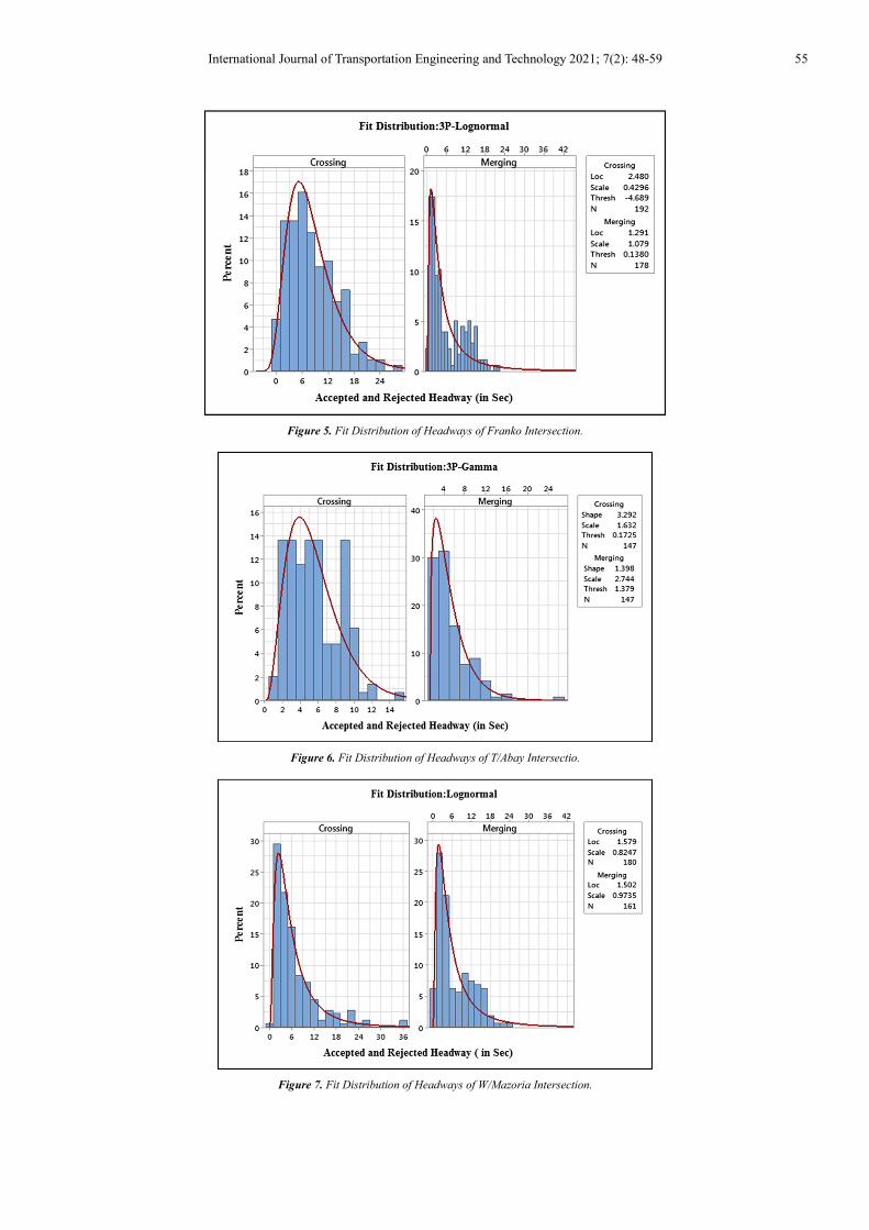
Exponential. From hypothesized distribution Table 5 shows
that best fit distribution of available gaps are; 3P-Lognormal,
3P Gamma and Lognormal distribution for Franko, Tikur
Abay and Wonji Mazoria intersection. And also for merging
maneuver type Lognormal is best fit distribution for Franko
intersection and 3P-Lognormal distribution for Tikur Abay
and Wonji Mazoria intersection. By considering AD values
and P- Values the researcher selected best distribution. AD is
statistics that is used to test distribution. For a significance
level of 0.05 the distribution which has small AD value or
less than critical value as taken best distribution. Illustration:
The null and the alternative hypothesis for goodness of fit
are;

54 Fikedu Rage Faye: Estimation of Critical Gap Using Maximum Likelihood Method at Unsignalized
Intersection: A Case Study in Adama City, Ethiopia
H0: the data follow the specified distribution; and H1: the
data do not follow the specified distribution, Where H0 and
H1 null and alternative hypothesis respectively. From seven
hypothesized distributions for Franko intersection 3P-
Lognormal distribution has been selected as first rank
Table 6. Summary of Goodness of Fit.
Intersection Distribution Turning Left (Crossing) Turning Right (Merging)
Parameters AD Values P-Values Best Fit Parameters AD Values P-Values Best Fit
Franko
Normal µ=8.37
σ=5.44 2.08 0.005
3P Lognormal
µ=6.08
σ=5.31 6.55 <0.005
3P Lognormal
Lognormal ɵ=1.82 λ=0.90
4.23 0.005 ɵ=1.35 λ=1.02
2.32 <0.005
3P Lognormal ɵ=2.48
λ=0.4 δ=-4.69
0.71 0.05 ɵ=1.29
λ=1.08 δ=0.14
2.18 0.05
Gamma β=1.8
λ=4.62 1.07 0.01
β=1.25
λ=4.86 3.25 <0.005
3P Gamma
β=2.60p
λ=4.21 δ=-0.29
0.82 0.05
β=1.01
λ=5.72 δ=0.33
2.24 0.05
Exponential µ=8.37 7.58 0.003 µ=6.08 2.63 <0.003
2P Exponential λ=8.09
δ=0.28 6.12 0.010
λ=5.75
δ=0.32 2.20 <0.010
Tikur Abay
Normal µ=5.54 σ=2.80
1.94 0.0005
3P Gamma
µ=5.22 σ=3.55
7.76 <0.0005
3P Lognormal
Lognormal ɵ=1.56 λ=0.57
1.53 0.0005 ɵ=1.47 λ=0.58
1.51 <0.0005
3P Lognormal ɵ=2.40 λ=0.35
δ=-2.61
1.16 0.05 ɵ=1.10 λ=0.80
δ=1.09
0.54 0.05
Gamma β=3.57
λ=1.55 1.01 0.014
β=2.97
λ=1.76 2.98 <0.005
3P Gamma β=3.29 λ=1.63
δ=0.17
1.00 0.05 β=1.398 λ=2.744
δ=1.379
1.06 0.05
Exponential µ=5.54 15.36 0.003 µ=5.22 13.46 <0.003
2P Exponential λ=4.83
δ=0.70 9.92 0.010
λ=3.77
δ=1.44 1.86 <0.011
W/Mazoria
Normal µ=6.81,
σ=6.24 11.36 0.005
Lognormal
µ=6.66,
σ=5.38 6.66 <0.005
3P Lognormal
Lognormal ɵ=1.57 λ=0.82
0.34 0.496 ɵ=1.50 λ=0.97
1.67 <0.005
3P Lognormal ɵ=1.37
λ=0.99 δ=0.60
0.37 0.05 ɵ=1.61
λ=0.86 δ=-0.33
1.83 0.05
Gamma β=1.61 λ=4.21
1.92 0.005 β=1.41 λ=4.72
1.95 <0.005
3P Gamma
β=0.99
λ=5.88 δ=0.96
0.35 0.05
β=1.33
λ=4.94 δ=0.11
1.78 0.05
Exponential µ=6.81 4.62 0.003 µ=6.66 2.55 <0.003
2P Exponential λ=5.87
δ=0.93 0.35 0.250
λ=6.47
δ=0.19 1.86 0.012
Note: µ (mean), σ (St.Dev), ɵ (location), β (Shape), λ (Scale) and δ (Threshold) are parameters used in testing goodness of fit
Table 7. Best fit Accepted and Rejected Gap distribution for Study Area.
Distribution Kolmogorov Smirnov Anderson Darling Chi-Squared
Statistic Rank Statistic Rank Statistic Rank
Exponential 0.15517 7 7.5735 7 39.503 7
Exponential (2P) 0.14212 6 6.0813 6 34.411 6
Gamma 0.07048 3 1.886 3 9.6535 3
Gamma (3P) 0.06252 2 0.81836 2 11.575 4
Lognormal 0.11147 5 4.2279 5 21.288 5
Lognormal (3P) 0.05102 1 0.07102 1 6.3458 1
Normal 0.08691 4 2.08 4 7.8164 2
International Journal of Transportation Engineering and Technology 2021; 7(2): 48-59 55
Figure 5. Fit Distribution of Headways of Franko Intersection.
Figure 6. Fit Distribution of Headways of T/Abay Intersectio.
Figure 7. Fit Distribution of Headways of W/Mazoria Intersection.

56 Fikedu Rage Faye: Estimation of Critical Gap Using Maximum Likelihood Method at Unsignalized
Intersection: A Case Study in Adama City, Ethiopia
The standard deviation controls the spread of the
distribution. A smaller standard deviation indicates that the
data is tightly clustered around the mean; the distribution
peak values is taller. A larger standard deviation indicates
that the data is spread out around the mean; the distribution
curve flatter and wider.
The peak values show variance which indicates that how
the data distribution are more concentrated to mean values or
not. Basic statistical characteristics of waiting time for two
maneuver types (merging and crossing) has been shown by in
the Table 8. Consider average waiting time of minor road
vehicles to cross and merge to major road, the vehicles that
are merging to major road have less waiting time means
drivers uses even available less gaps compared to these
drivers who are crossing the major road and turning to the
right.
Table 8. Statistical Properties of Waiting Time for with maneuver type in seconds.
Intersection’s Minimum Maximum Mean
Crossing Merging Crossing Merging Crossing Merging
Franko 1.00 .00 25.85 12.87 10.54 6.46
T/Abay .06 .27 23.20 19.91 12.38 11.11
W/Mazoria 1.04 .00 19.72 14.27 9.88 6.70
As per collected data average waiting time for merging
maneuver are 6.46sec, 11.12sec and 6.70sec for Franko,
Tikur Abay and Wonji Mazoria intersection respectively. And
also for traffic turning the right, 10.54, 12.38, and 9.88 sec.
Table 8 provides that distribution fit for waiting time on
minor road for both left turning and right turning drivers. It
has been shown that lognormal distribution is selected for the
left turning drivers. And also for the merging to major road
3P-Gamma distribution is best fit to explain distribution of
waiting time. Non parametric K-S test was used to test and
validated estimated model at 95% confidence interval.
3.2. Critical Gap Estimation
As per literature review most common methods used by
many researchers in determination of critical gap were:
Maximum likelihood method, Raff method, Green shield
method, The Lag method, Harder’s method, Logit method,
and Wu’s Method. In this study Maximum likelihood method
was used in estimation of critical gap for drivers for selected
unsignalized in Adama city. The maximum likelihood
method of estimating critical gap is based on the fact that a
driver's critical gap is between the range of his largest
rejected gap and his accepted gap [9]. Density function
distribution for the critical gaps must be assumed between
the largest rejected gap and accepted gap and used a log-
normal distribution for the critical gaps. This distribution is
skewed to the right and has non-negative values, as would be
expected in these circumstances. Drivers that are turning to
right and turning to left from minor road have different
critical gaps. In this paper two cases have been studied were
critical gap for merging to major road and crossing major
road turn to left be estimated separately by maximum
likelihood method. As Dutta, M. M. [10] forwarded the
parameters of distribution function of the critical gaps, the
mean (µ) and variance (σ2), are obtained by maximizing the
likelihood function.
L=∏ [����� − ����]� ��
Where, L=maximum likelihood function, ai=logarithm of
the accepted gap of driver i, ri=logarithm of the maximum
rejected gap of driver i, F (ai) and F(ri)=cumulative
distribution functions for the normal
Distribution of accepted and rejected gap respectively
Figure 8. Empirical Cumulative Distribution Function (ECDF) of Gaps of Franko.

International Journal of Transportation Engineering and Technology 2021; 7(2): 48-59 57
Table 9. Estimated Maximum Likelihood Parameters and Critical Gaps.
Intersection Maneuver Type Mean St.Dev Std.2 E(tc)
Franko Crossing 0.71 0.10 0.01 5.17
Merging 0.69 0.15 0.02 5.03
T/Abay Crossing 0.63 0.11 0.01 4.32
Merging 0.57 0.13 0.02 3.79
W/Mazoria Crossing 0.59 0.14 0.02 3.96
Merging 0.68 0.14 0.02 4.88
Empirical cumulative distribution function of accepted,
maximum rejected and critical gap at Franko intersection has
been shown on Figure 8. The critical gap distribution is
between accepted gap and maximum rejected gap. It has been
observed that 50% of accepted gap for the traffic that are
Turning to left (crossing) are less than 18sec and that of
rejected gap is less than 15sec. All gaps accepted or rejected
as per data collected for major stream of Tikur Abay is less
than 40sec. Estimated critical gaps for unsignalized intersection has
been shown on the Table 10. These values can bes used
directly in determination of capacity and delay. It is observed
that critical gaps available for drivers at Tikur Abay
intersection is least in both manuver type. This shows that the
driver uses more gaps to cross and merge to major road.
Critical gap at Franko intersection for the drivers that are
crossing major roads is largest estimated values which is
5.17sec. Critical gap has been estimated by equation of;
E(tc)= �µ+0.5σ
2
, where, E(tc): Expected critical mean,
µandσ are parameters of normal distribution of PDF of f(ai)
and f(ri) and ai and ar is logarithmic value of accepted and
rejected gaps respectively.
Table 10. Estimated Critical Gap for Traffic Turning to the Left and Right.
Intersection Opposing
Volume
Minor Road
Volume
Speed (in
kmph)
Waiting Time (in sec) Estimated Critical gap
Crossing Merging Crossing Merging
Franko 1,157.00 881.00 30.00 12.67 7.54 5.17 5.03
T/Abay 1,233.00 606.00 30.12 8.36 14.81 4.32 3.79
W/Mazoria 1,531.00 1,110.00 28.70 7.44 8.69 3.96 4.88
Average 4.56 4.48
4. Discussion
Headway distribution is important in traffic modelling and
simulation. Several studies have been conducted on headway
distribution under heterogeneous traffic conditions. Arrival
patterns and direction of turning affects distribution of
headway. This study revealed headway distribution for
different ranges of flow rates for selected unsignalized
intersection in Adama city. It is observed that Gamma and
exponential distribution were found to be best model for low
traffic flow level which is 600-1200PCU/Hr. And also from
moderate to higher flow rate (1200-2500) PCU per hour
lognormal distribution was found appropriate model in this
paper. This finding is similar with the study conducted in
India in Assam by Farah et al., H [11] and in Mumba Al-
Obaedi, J. i by [4]. Another study that has been conducted in
India by Abhishek, O., & Marko A. A. Boon, R.-Q [2]
showed that log-logistic and normal distribution were found
best model at moderate flow level and Pearson distribution
for peak state flow. Difference of selected distributions may
arise due to traffic flow condition and ranging of traffic flow
rate from countries to countries.
One important parameter of traffic flow characteristic
focused in this study was critical gap. By using maximum
likelihood method driver’s critical gaps for selected
intersection of Adama city has been estimated. The current
study found that the critical gap of left turning drivers are
5.17, 4.32 and 3.96seconds for flow rates of 1100, 1300 and
1500PCU/Hr. respectively. For the driver that merging to
major road estimated critical gaps were 5.03, 3.79 and 4.88
seconds for stated traffic flow rates. Average estimated
critical gap for left turning in this study is 4.56sesc and for
right turning vehicles is found to be 4.48sec. The same study
has been conducted in Malaysia by Gavulova, A. Gavulova,
A [12] which is revealed critical gap for left turning drivers
has been found to be 3.3sec and 4.2sec for right turning
vehicles. Thus it seems possible that, these results could be
due to the fact that as the flow rate increase critical gap of
drive leads to decrease. Another’s similar studies that has
been conducted in different countries has been shown in the
Table 11.
Table 11. Comparison of Estimated Critical by different Authors.
Paper/Author Name Major Road Lane Average Speed Critical gaps (in Sec)
Left Turn Right Turn Average
This study/2020 2 30kmph 4.56 4.48 4.52
Wan Hashim/2007 1 Base value 4.0 3.30 3.6
Multilane 4.20 3.30 3.72
HCM/2010 2 Base value 7.1 6.2 6.65
4 Base value 7.5 6.5 7.20
(Andyka et al./2011 2 33kmph 3.29 3.58 3.43
Zongzhong et al./1999 2 - 4.7 4.4 4.55
See that above Table 11 critical gap for merging traffic is
4.48 and for crossing major road 4.56. It is close to that of
[15, 6] and [16] studies. This may be shows the similarities
of traffic flow characteristic with this area of study.

58 Fikedu Rage Faye: Estimation of Critical Gap Using Maximum Likelihood Method at Unsignalized
Intersection: A Case Study in Adama City, Ethiopia
Discrepancies of this study and other study has been also
shown on the Table 11 Critical headway (gaps) of developed
country like America which is mentioned in R. Morris, M.
[14] are different from that of developing country. For
example, study done by Gavulova, A. [12] in Malaysia is
more similar with this study. In general, the critical gaps need
to merge or turning right is less than that of turning left.
5. Conclusion and Recommendation
5.1. Conclusion
This paper presents a detail study of available headway
distribution, waiting time characteristics of unsignalized
intersection under mixed traffic condition and weak lane
disciplined urban unsignalized intersection.
Among hypothesized models lognormal distribution
selected and validated for higher flow rate like Franko
intersection and Gamma distribution is best fit for low flow
rate like Tikur Abay Intersection. By considering two
alternatives turning left (crossing) and turning right (merging
to major road) in determination drivers critical gap estimation
were done.
For the drivers who are turning to right computed critical
gaps for Franko, Tikur Abay and Wonji Mazoria intersection
were 5.17sec, 4.32sec and 3.96sec respectively.
And also the waiting time of drivers that are turning to left
for three selected intersections were about 26sec, 24sec and
20sec. From the developed nonlinear model traffic turning to
left moving with average speed 30kmph, average headway of
10sec and minor road traffic volume 2000PCu/Hr., increasing
25% major road traffic volume makes to double waiting time
on minor road. Increasing major road traffic volume by 50%
makes to quadruple waiting time.
For low flow rates less than 500PCU/Hr., average speed of
20kmph and large headway more than 25sec waiting time not
more affected by traffic volume on major road. For the
turning to right the minor road volume has high influence on
waiting time. Generally Safe crossing of vehicles and
merging of vehicles from minor road to major road, for the
lane width less than 3.6m and the traffic volume on the major
road should not be more than 2200PCU/Hr. and the critical
headway on the major road should not be less than 4.56sec
and 4.48sec respectively.
5.2. Recommendation
In this paper Headway distribution and critical gaps for
drivers has been estimated. And also waiting for characteristics
of drivers to accept or reject gaps has been investigated. For
forthcoming researchers and professionals, the author of this
paper recommended the following areas of study related to this
investigation for forthcoming researchers.
1) Influence of driver’s behavior (i.e. aggressiveness,
drugs and alcoholic, age, gender on gap acceptance at
unsignalized intersection.
2) Influence of distress like rutting, potholes etc. on gap
acceptance at unsignalized intersection.
3) Impact of topography and geometric layout of
intersection on gap acceptance at uncontrolled
intersection.
4) Skid resistance and surface deflection on gap
acceptance at uncontrolled intersection under mixed
traffic condition.
For drivers and road users:
a) Drivers shouldn’t take gaps less suggested critical of
4.36sec for left turning and 3.79 for right turning.
b) Pedestrians should use their facilities to cross or to
merge to major road
For Policy makers and Professional
a) They should prepare guideline which gives more
understanding for driver and road users
b) Properly regulate traffic to reduce waiting time by
posting, speed limit less than 30kmph, critical gap
greater than suggested (3.79sec), installation of signal
specially on Tikur Abay intersection.
References
[1] Abd-Elaziz, A., & Abd-Elwahab, S. (2017). The Effect of Traffic Composition on PCU Values and Traffic Characteristics on The Northern Arc of The first Ring Road around Greater Cairo. IOSR Journal Of Humanities And Social Science (IOSR-JHSS), 01-17.
[2] Abhishek, O., & Marko A. A. Boon, R.-Q. (2017). A single-server queue with batch arrivals and semi-Markov services. Queueing Syst, 217–240.
[3] Akhilesh et al., M. K. (2014). Study on Speed and Time-headway Distributions on Two-lane Bidirectional Road in Heterogeneous Traffic Condition. 11th Transportation Planning and Implementation Methodologies for Developing Countries, 428-438.
[4] Al-Obaedi, J. (2016). Estimation of Passenger Car Equivalents for Basic Freeway Sections at Different Traffic Conditions. World Journal of Engineering and Technology, 1-17.
[5] Amin, H. J. (2015). A review of Estimation approaches at uncontrolled intersection in case of heterogeneous traffic conditions. 5-9.
[6] Andyka, K., & Haris, N. (2011). Critical Gap Analysis of Dual Lane Roundabouts. Procedia Social and Behavioral Sciences, 709-717.
[7] Arvind et al., M. (2008). Macroscopic Review of Driver Gap Acceptance and Rejection Behavior in the US - Data Collection Results for 8 State Intersections. Minessota: Intelligent Transportation Systems Institute.
[8] Bartin et al., O. (2017). Simulation of Vehicle ’ Gap Acceptance Decision Using Reinforcement Learning. Uludağ University Journal of The Faculty of Engineering, 161-178.
[9] Doddapaneni et al., A. (2017). Multi Vehicle-Type Right Turning Gap Acceptance and Capacity Analysis at Uncontrolled Urban Intersections. Periodica Polytechnica Transportation Engineering, 1-9.
[10] Dutta, M. M. (2018). Gap acceptance behavior of drivers at uncontrolled T-intersections under mixed traffic conditions. Journal of Modern Transportation, 119-132.

International Journal of Transportation Engineering and Technology 2021; 7(2): 48-59 59
[11] Farah et al., H. (2009). A passing Gap Acceptance model for two lane rural highway. Transportmetrica, 159-172.
[12] Gavulova, A. e. (2012). Use of statistical techniques for critical gaps Estimation. “Reliability and Statistics in Transportation and Communication” (pp. 20-26). Zillina: Transport and Telecommunication Institute.
[13] Maurya, A. (2015). Speed and Time headway Distribution Under Mixed Traffic Condtion. Journal of Eastern Asia Society for Transportation Studies, 1-19.
[14] R. Morris, M. (2010). Highway Capacity Manual (Vol. I). Washington DC: Transportation Research Board Committee.
[15] Wan Ibrahim, W. (2007). Estimating Critical Gap Acceptance For Unsignalized T-Intersection Under Mixed Traffic Conditions. Procedings of Eastern Asia Society For Transportation Studies, 2-13.
[16] ZongZhong et al., T. (1999). Implementing the maximum likelihood methodology to measure a driver's critical gap. Transportation Research Part A 33, 187-197.