LEHIGH UNIVER ITY

Prestress Losses in Pretensioned

Concrete Structural Members

ESTIMATION OF CONCRETE STRAINSAND

PRESTRESS LOSSES INPRETENSIONED MEMBERS

FRITZ ENGINEEFm«a·LAa~ltJrto·RY .. l'8R~ItY'. '.

byHai-Tung Ying

Erhard Schultchen

Ti Huang

Fritz Engineering Laboratory Report No. 339.7

Lehigh University

Research Proiect 339 Reports

PRESTRESS LOSSES IN PRETENSIONED

CONCRETE STRUCTURAL MEMBERS

COMPARATIVE STUDY OF SEVER~AL CONCRETES REGARDING THEIRPOTENTIALS F'OR CONTRIBUTING TO PRESTRESS LOSSES.

Rokhshar r A. and Huang r T' r F. l. Report 339.1 r June 1968

CONCRETE STRAINS IN PRE-TENSIONIED CONCRETE STRU'CTURALMEMBERS - PRELIMINARY REPORT. Frederickson r D. and Huang, T.,F. L. Report 339.3, June 1969

RELAXATION LOSSES IN 7/16 in. DIAMETER SPECIAL GRADEPRESTRESSING STRANDS. Schultchen, E. and Huang, T.,F. L. Report 339.4, July 1969

RELAXAliON LOSSES IN STRESS-RELIEVED S,PECIAL GRADEPRESTR,ESSING STRANDS. Batal, R. and Huang, T.,F. L. Report 339.5, April 1971

RELAXATIO,N BEHAVIOR OF PRESTRESSING STRANDS.

Schultchen r E., Ying, H.-T. and Huang, T.,F. L. Report 339.6, March 1972

ESTIMATION OF CONCRETE STRAINS AND PRESTRESS LOSSES IN,PRETENSIONED MEMBERS. Ying, H.-T., Schultchen, E. and Huang, T.,

F. L. Report 339.7, May 1972

'1- ,

COMMONWEALTH OF PENNSYLVANIA

Department of Transportation

Bureau of Materials, Testing and Research

Leo D. Sandvig ~ DirectorWade L. Gramling - Research Engineer

Kenneth L. Heilman - Research Coordinator

Project 66-17: Prestress Losses in PretensionedConcrete Structural Members

ESTIMATION OF CONCRETE STRAINS

and

PRESTRESS LOSSES IN PRETENSIONED MEMBERS

by

Hai-Tung YingErhard Schu1tchen

Ti Huang

The contents of this report reflect the views of the authorswho are responsible for the facts and the accuracy of the datapresented herein. 'The contents do not necessarily reflectthe official views or policies of the Pennsylvania Departmentof Transportation, the Federal Highway 'Administrati6n~ or theReinforced Concrete Research Council. This report does notconstitute a standard, specification, or regulation.

LEHIGH UNIVERSITYOffice of Research

Bethlehem, Pennsylvania

May, 1972

Fritz Engineering Laboratory Report No. 339.7

TABLE OF CONTENTS

ABSTRACT

1. INTRODUCTION

2. DATA REDUCTION AND ANALYSIS

2.1 Method of Analysis

2.2 Data Reduction

2.3 Two-Dimensional Analysis

2.4 Three-Dimensional Analysis

3. COMPONENTS OF CONCRETE STRAINS

3.1 Components of Concrete Strains

3.2 Elastic Shortening

3.3 Shrinkage Strain

3.4 Creep Strain

3.5 Estimation of Concrete Stress, fC3

4. COMBINED CONCRETE AND STEEL STRESS-STRAIN-TIMERELATIONSHIP

4.1 Introduction

4.2 Steel Functions

4.3 Concrete Functions

4.4 Steel-Concrete Relationships

5. DISCUSSION OF RESULTS AND SUMMARY

5.1 Application of Prediction Method

5.2 Comparison of Predicted Results (PRELOA)and Three-Dimensional Results (CUNIFB)

5.3 Effects of Types of Concrete and InitialPrestress

ii

vi

1

3

3

3

4

6

9

9

9

10

11

13

15

is

15

1617

22

22

23

23

Page

5.4 Summary 24

6. ACKNOWLEDGMENTS 25

7 e TABLES 26

8. FIGURES 39

g. REFERENCES 45

APPENDIX - NOTATIONS 46

iii

LIST OF TABLES

Table

.1 Two-Dimensional Results for Uniformly Stressed 27Specimens

2 Two-Dimensional Results for Shrinkage Specimens 28

3 Three-Dimensional Results fov Uniformly Stressed 29Specimens

4 Three-DimensionaL Results for Shrinkage Specimens 29

5 Coefficients of Shrinkage Function 30

6 Predicted Shrinkage Strain at 100 Years 30

7 Coefficients of Creep Function 31

8 Predicted Creep Strain at 100 Years 31

9 Comparison of f for CUNIFC and PRELOA83

32

10 Values of k 1 , kg, k s and ~ for Various Series ofSpecimens

1J. :.Prestress Losses Predicted by PRELOA

12 Predicted Concrete Strains at 10 Days

13 Predicted Concrete Strains at 100 Days

14 Predicted Concrete Strains at 1000 Days

15 Predicted Concrete Strains':at 100 Ye,a~~rl.

iv

33

34

35

36

37

38

Figure

1

2

3

4

5

LIST OF FIGURES

Stress Distributions for Rectangular Specimens

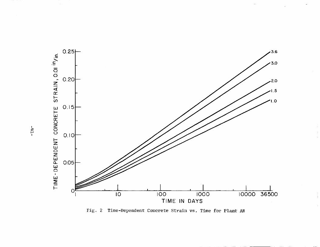
Time-Dependent Concrete Strain vs. Time forPlant AB

Time-Dependent Concrete Strain VB. Time forPlant CD

Shrinkage Strain VB. Time for Plant AB

Shrinkage Strain vs. Time for Plant CD

v

40

41

42

43

44

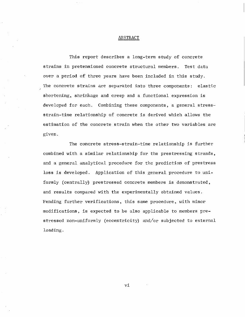
ABSTRACT

This report describes a long-term study of concrete

strains in pretensioned concrete structural members. Test data

over a period of three years have been included in this study.

The concrete strains are separated into three components: elastic

shortening, shrinkage and creep and a functional expression is

developed for each. Combining these components, a general stress­

strain-time relationship of concrete is derived which allows the

estimation of the concrete strain when the other two variables are

given.

The concrete stress·-strain-time relationship is further

combined with a similar relationship for the prestressing strands,

and a general analytical procedure for the prediction of prestress

loss is developed. Application of this general procedure to uni­

formly (centrally) prestressed concrete members is demonstrated,

and results compared with the experimentally obtained values.

Pending further verifications, this same procedure, with minor

modifications, is expected to be also applicable to members pre­

stressed non-uniformly (eccentricity) and/or subjected to external

loading.

vi

1. INTRODUCTION

The research project "Prestress Losses in Pretensioned

Concrete Structural Members" was initiated in 1966 with the ob ..

jective of establishing a rational basis for the prediction of

prestress losses in pretensioned highway bridge members used in

Pennsylvania. In two separate phases of the project, concrete

and steel specimens are being tested for the several major

factors contributing to prestress losses. To date, several re­

ports have been issued de'scribing the experimental work, and pre­

senting preliminary results and conclusions.

Prestress losses due to elastic shortening, shrinkage

and creep' in concre'te were investigated by t,esting concrete 'speci­

mens. From a preliminary study of the loss characteristics of

several concretes (Ref. 1), two plants had been selected to pro­

duce these specimens, one with concrete exhibiting the ,highest

loss characteristics (plant AB) and the other the lowest (plant

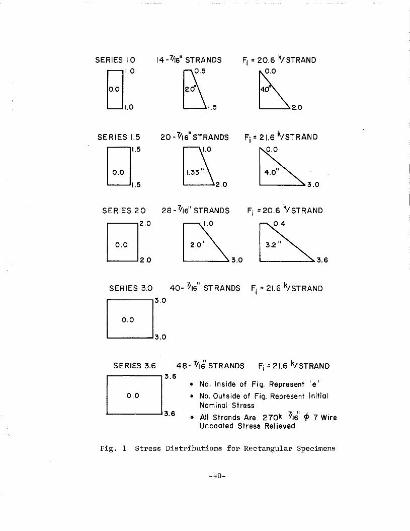
CD). A total of twenty-two prestressed specimens were fabricated

at each plant. By controlling the number and location of pre­

stressing:strands, variations of average prestress level and lat­

eral stress gradient were obtain~d, as shown in Fig. 1. In addi­

tion, twenty unprestressed shrinkage specimens were also fabri­

cated at each plant. The majority of these specimens contain un­

stretched strands corresponding to the various prestressed speci­

mens. There is also a series of shrinkage specimens with no

-1-

strands in them. A detailed description of the test specimens

and experiment was given in Ref. 2.

The preliminary results, at the end of one year, of

this phase of the experiment have been presented in Ref. 2. This

present report contains the final results based on data from the

shrinkage and the uniformly stressed specimens. Test data over a

period of three years have been included in the analysis.

In Ref. 3 a concept of stress-strain-time relationship

was introduced and applied to the steel relaxation data. This

same concept will be applied in this report to the concrete

strain data. The concrete and steel stress-strain-time relation­

ships will then be combined to form a basis for the prediction of

prestress losses. Numerical results of prestress losses pre­

dicted by this method will be shown, and compared with the e~peri­

mental data.

In Chapter 2, measured concrete strains from the shrink-

age and uniformly prestressed specimens are analyzed two- and

three-dimensionally to determine the most suitable time and stress

function forms. Chapter 3 contains the analysis of the separate

components of concrete strain, using the function form selected in

Chapter 2. The development of the complete concrete stress-strain­

time relationship and of the general analysis procedure are pre­

sented in'Chapt~r 4.

-2-

2. DATA REDUCTION AND ANALYSIS

2.1 Method of Analysis

The procedure of analysis used on the concrete strain

data is similar to that which was adopted in the development of

the steel stress~strain-time relationship (Ref. 3). First of

all, a two-dimensional analysis was performed. The concrete

strain data for each given initial concrete stress were analyzed

as a function of time only. After the selection of the time

function, the data from all specimens were then analyzed TTthree~

dimensionallyTT, treating both the initial concrete stress and the

time as independent variables. In this chapter, the initial

concrete stress refers to the nominal concrete stress obtained by

dividing the total prestress force by the gross sectional area· of

the member.

2.2 Data Reduction

Both shrinkage and uniformly stressed specimens data

were reduced in the same manner. The readings taken immediately

after the transfer of prestressing force were used as the bases

of reference. To determine the concrete strains at subsequent

times, the corresponding readings were subtracted from these ini­

tial readingso The differences represented respectively the

change of gage length due to shrinkage, in the case of shrinkage

specimens, and that due to the combination of shrinkage, creep

-3-

and relaxation, in the case of prestressed specimens. By using

the after release readings, rather than the before release read­

ings, as the bases of reference, the effect of elastic shortening

was excluded.

All data used in both two-dimensional and three­

dimensional analysis were reduced in the same manner as described

in the preceding paragraph.

2.3 Two-Dimensional Analysis

The time-dependent natures of concrete strain and steel

relaxation are quite similar. The same 1tessential conditions TT

listed in Ref. 3 should also be satisfied by the time function of

concrete losses. Therefore, the same test functions used in the

two-dimensional analysis of steel relaxation were also used in

the analysis of concrete strain data:

:a1. Set) = At + Az log t + As (logt)

2 . S (t) = A1 + A a log t

3.

4.

S (t)

S (t)

= A 1 + A ~ log (t + 1)

= A1

+ Aa log (t + 1)

a+ Aa [log (t + 1) ]

A computer program, CUNIFA, was developed to perform

the two-dimensional regression analysis, using the method of

least squares. Strain data from a single se~ies of specimens

(consisting of two concrete specimens, and up to 40 strain

-4-

readings at any given time) were used, and time after transfer of

prestress was the only independent variable.

The same criteria used in Ref. 3 for selecting the best

time function were used. The functions were evaluated primarily

on the basis of their stability, that. is, whether their long-term

predictions and behavior were strongly affected by the inclusion

and exclusion of data near either end of the test period. Stand­

ard' errors were also compared to see how well each test function

approximated the data.

Functions (1) and (3) were affected strongly by expe~i­

mental data near the beginning of the test period, and therefore

were rejected. Both functions (2) and (4) were relatively insen­

sitive to the variations of the test period, although the stand­

ard errors were slightly higher than those of functions (1) and

(3) because of their ~imp~er forms. Between these two, function

(4) showed less sensitivity to "changes :of.(th~' beginning timel, .

of the test period and also resulted in lower stanrnard errors.

Therefore, function (4) was considered to be the best time func­

tion, and was selected to be used in the three-dimensional analy­

sis~ Incidentally, function (4) is the same time function which

was selected for relaxation of steel.

Values of predicted strains at 100 years, and standard

errors for the diffe~ent series of uniformly stressed and shrink­

age specimens are listed in Table 1 and 2 respectively.

-5-

2.4 Three~DimensionalAnalysis

In the two-dimensional analysis, the data analysis was

restricted to time-dependent functions which allowed the predic-

tion of concrete strains for single sets of data corresponding to

a particular level of initial concrete stress. A logical exten-

sion of this concept would be to include the initial nominal

stress as a second independent variable besides time.

As in Ref. 3 the stress-dependent trial functions were

aobtained from linear combinations of 1, f., f. , where f. was the

1 1 1

initial concrete stress.

1. S (f.)1

= B1

+ B f..a 1

2+ B f.3 1

2. S (f.) = B1

+ B f.1 2 1

3 • S (f.)1

a+ B f.

2 1

In a fairly general form the concrete strains as a

function of initial stress and time can be expressed as

SCf. ,t)1

·M= ~

rn=i

N~

n=l

where F Cf.) are subfunctions of the initial stress f. only andm 1 ].

T (t) are subfunctions of time t. With the time-dependent func­n

tion already selected by the two-dimensional analysis, only four

functions were tested in the three-dimensional analysis:

-6-

2+ f i [C5 + Cs log (t + 1) ]

2. S (f. ,t) ~ C1 + C~ log (t + 1) + f. [C + Clog (t + 1) ]1 ~ 134

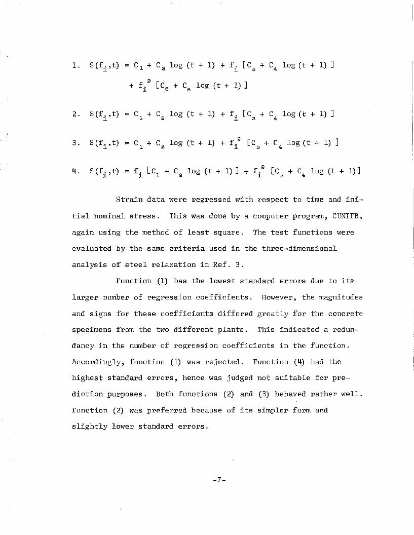
Strain data were regressed with respect to time and ini-

tial nominal stress. This was done by a computer program~ CUNIFB,

again using the method of least square. The test functions were

evaluated by the same criteria used in the three-dimensional

analysis of steel relaxation in Ref. 3.

Function (I) has the lowest standard errors due to its

larger number of regression coefficients. However, the magnitudes

and signs for these coefficients differed greatly for the concrete

specimens from the two different plants. This indicated a redun-

dancy in the number of regression coeffici.ents in the function 0

Accordingly, function (1) was rejected. Function (4) had the

highest standard errors, hence was judged not suitable for pre-

diction purposes. Both functions (2) and (3) behaved ~ather wello

Function (2) was preferred because of its simpler form and

slightly lower standard errors.

-7-

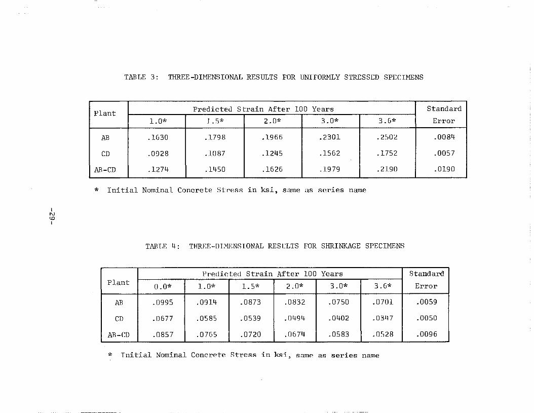
With the selected function (2), three regression analy­

ses were performed, one for each plant separately and the third ,:

for both plants combined. The standard errors together with the

predicted strains at 100 years for different initial concrete

stresses for the uniformly stressed and shrinkage specimens are

listed in Table 3 and 4 respectively. The functions for the uni­

formly·stressed and shrinkage specimens from plant AB and plant

CD are also plotted in Figs. 2 - 5.

-8-

3. COMPONENTS OF CONCRETE STRAINS

3.1 Components of Concrete Strains

In a prestressed concrete member, the concrete strains

contributing to the prestress loss can be separated into three

components: elastic shortening, shrinkage and creep. In this

chapter, the effect of each was studied separately and a predic-

tioD formula developed for the ~espective components. By com-

bining the three components the total concrete strain can be

predicted.

The variables and units used in the development of all

the prediction formulas were:

s: concrete strain, in 0.01 :i!n.,flin/(ela'sti~,'shrihkage

and creep components designated by subscripts el,

sh and aI', respectively)

f: concrete stress, in ksic

f: steel stress, in~sis

t: time after transfer of prestress, in days

3.2 Elastic Shortening

In the prediction of elastic shortening, the idealized

linear elastic stress-strain relationship of concrete was utilized.

S (f) = C' fel C l' C

-9-

(3-1)

where = 100iEc

E = elastic modulus of concrete at time of transfer,c

in ksi

Standard cylinder tests were used to determine the se-

cant modulus of the concretes studied in this project. The aver-

age values for plant AB, plant CD, and their average 'were 4000

ksi, 4750 ksi, and 4350 ksi, respectively.

It should be pointed out that the concrete stress, f ,c

in equation (3-1) refers to that at any arbitrary time, t, after

the transfer of prestress. As such, the equation includes the ef-

fect of elastic rebound of concrete due to the gradual decrease

of concrete stress.

3.3 Shrinkage Strain

As described in Chapter 2, one of the independent vari-

abIes for the three-dimensional analysis was' the "nominal concrete

stress TT , obtained by dividing the total tensioning force in

strands by the gross sectional area of the specimen. For the

shrinkage data, the nominal stress in the companion uniformly

stressed specimens was used in the analysis. However, as these

shrinkage specimens were actually not prestressed, a more logical

choice of parameter would be the amount of reinforcement, reflect-

ing the restraining effect of steel on the shrinkage of concrete.

Therefore, in the final analysis of shrinkage data, the parameter

-10-

TT nominal concrete stress TT was replaced by the amount of reinforce­

ment (including both prestressing strands and non-prestressing

bars). The revised three-dimensional function takes the follow­

ing form,

Ssh.(~,t) = D1 + D,a log (t + 1) + ~ [D3

+ D4

log (t + 1) ] (3-2)

where

t

= amount of reinforcement, in percent of the

gross cross section area

= time after end of curing, taken as same as

time after transfer of prestress, in days

The shrinkage coefficients in equation (3-2) were deter­

mined separately for plant AB concrete, plant CD concrete and for

the two plants combined, and are listed in Table 5. The predicted

shrinkage strains at 100 years for various steel percentages are

listed in Table 6.

3.4 Creep Strain

The reduced strain data used in the three-dimensional

analysis of the uniformly stressed specimens included shrinkage

and creep of concrete as well as the elastic rebound of concrete

strain due to decreasing concrete stress. In order to isolate the

effect of creep, strains due to shrinkage and elastic rebound must

be deducted from the experimental values for total strain.

-11-

Shrinkage strains were calculated by equation (3-2). Elastic re-

bound was calculated by using the linear elastic stress-strain

relationship

where

S = Cll (f - f )er Ca C

S = elastic rebound strain, in 0.01 in/iner

(3-3)

f = concrete stress at transfer of prestress, in ksiC3

The creep strain of concrete Scr' was then calculated as

(3-4)

where Set = total strain of uniformly stressed specimens

For the estimation of the elastic rebound, and for the

regression analysis of creep strain data, concrete stress f atc

each data time must first be evaluated. This was accomplished by

first calculating the stress in steel strands by the steel stress-

strain-time relationship with strain and time known. The concrete

stress was then calculated from the equilibrium conditions 0

The concrete stress immediately after transfer of pre~

stress, f ,was also required in equation (3~3). It was esti­C3

mated by the method described in Section 3.50

A computer program, CUNIFC, was developed to perform the

necessary calculations and the regression analysis of the isolated

-12-

creep strain data. The ~egression function used was the same one

selected in the three-dimensional analysis.

S (f, t) = E1 + E~ log (t + 1) + f [E + E log (t + 1) ]cr C Q C 3 4(3-5)

where E"E ,E ,E are regression coefficients~. 2 3 4

The creep coefficients in equation (3-5) were determined

separately for plant AB concrete, plant CD concrete and for the

two combined, and are listed in Table 7. The predicted strains at

100 years for different constant concrete stresses are listed in

Table 8.

3.5 Estimation of Concrete Stress, fC3

For the concrete specimens used in this research project,

no direct measurement of steel stress (or strain) was possible

after detensioning of the prestressing bed. The stress condi-

tions immediately after transfer must therefore be estimated in-

directly. In computer program CUNIFC, the after-transfer stresses

were estimated in the following manner. As a first step, the

steel stress-strain-time relationship (Ref. 3) was used to evalu-

ate the relaxation loss for the time period from tensioning to im-

mediately before transfer. This calculated value, however, did

not reflect the effect of elevated temperature which existed dur-

ing this period of time. It is known that relaxation increases

rather substantially under continuous high temperature. On the

-13-

other hand, experimental data are not currently available for a

quantitative determination of the short-duration temperature ef-

feet during the curing period. An increase of 30% was assumed,

resulting in an estimated total relaxation loss before transfer of

from 4.2 to 4.7% of the initial steel stress for plant AB speci-

mens and from 3.8 to 4.3% for plant CD specimens. (The average

lengths of curing period were three days and two days for the two

plants, respectively.) To simplify calculations, an average value

of 4.5% was used for plant AB and 4.0% for plant CD. Subtracting

these values from the initial tensioning stress resulted in the

steel stress immediately before transfer, f .sz

The difference between the concrete strain readings

taken immediately before and after release of prestressing force

represented the elastic strain. Multiplying this elastic strain

by the elastic modulus of steel, taken as 28000 ksi, resulted in

the elastic loss of steel stress. Subtracting this elastic loss

from the steel stress immediately before transfer, f , the steelS2

stress after tranfer, f ,was obtained. The corresponding after­83

release concrete stress, f , was simply calculated from the equi­C3

librium condition between the steel and concrete stresses.

It will be noted later that in the general procedure for

prediction of prestress losses, a different procedure is used for

the estimation of after-transfer stress condition. Further com-

ments will be given in Section 4.4.

-14-

4. COMBINED CONCRETE AND STEEL STRESS-STRAIN-TIME RELATIONSHIP

4.1 Introduction

In this chapter, the functions separately developed for

steel (Ref. 3) and concrete (Chapter 3) are integrated to yield

the combined form of "concrete-steel tT stress-strain-time relation-

ship. The steel and concrete functions are recollected in Sections

4.2 and 4.3. Section 4.4 describes the linkage of the steel and

concrete stress-strain-time relationships, and outlines the pro-

cedure of the application of the combined relationship.

4.2 Steel Functions

The following steel functions were developed in Ref. 3.

(1) Stress-strain relationship

f (8) = { A1 + AaSs + A sa} f (4-1)sel S 3 S pu

(2) Relaxation loss of steel stress

L(S ,t ) = { Ss [B 1 + B:a log (t + 1) ]s s s

+ S .a [B3

+ B4

log (ts + 1) ] } f (4-2)s pu

(3) Stress-strain-time relationship

f (8 ,t ) = f . (8 ) - L (8 ,t )s s s sel S S S

= {A1

+ S [A - Bl - Bas a

2[A

3+ S - B3 - B4 logS

log (ts + 1) ]

(ts + 1) J} f pu (4-3)

-15-

= steel stress, in ksi

= relaxation loss, in ksi

= steel strain, in 0.01 in/in

= time after stretching of strands, in days

= guaranteed ultimate strength of steel,

in ksi

where Ss

t s

L

f s

f pu

= regression coefficients of stress-strain

curve of steel

Bl

,Ba ,Bs ,B4

= regression coefficients of relaxation of

steel

The applicability of the stress-strain-time relationship

equation (4-3) is restricted to time values from approximately one

day to 100 years and to initial stress values in the range from

0.5 to 0.8 of the ultimate tensile strength.

4.3 Concrete Functions

(1) Elastic shortening

Sel (~c) = Clfe(4.n4)

(2) Shrinkage

Ssh(f.L,tc

) = D l + D,a log (tc

+ 1) + f.L [D3 + D4 log (tc + 1) ] (4-5)

-16-

(3) Creep

(4) Total concrete strain

S (J.L, f ,t ) = Se 1 + S h + Sc c c s cr

= [D]. + El

+ J.kD s + (Da + Ea + J.kD4

) log (tc

+ 1) ]

+ [C + E + E log (t + 1) ] f1 3 4 C C

(4-7)

Equations (4-4), (4-5) and (4-6) are identical to equa-

tions (3-1), (3-2) and (3-5), respectively, which were developed

in Chapter 3. All parameters have been defined previously, except

that the time parameter is now denoted by t. The total concretec

strain was obtained by simply combining the individual concrete

components. The range of applicability of equation (4-7) is, in

accordance to the data source, for t to be from approximately onec

day to 100 years, and for f to be below 3 ksi.c

4.4 Steel-Concrete Relationships

Combining the stress-strain-time relationships of steel

and concrete materials, a general procedure for the prediction of

stress conditions in a prestressed concrete member can be estab-

listed. Initially, the development of this general procedure was

based on the uniformly (centrally) prestressed specimens. For

these specimens, the stress, strain and time parameters for the

two materials are related by equations (4-8), (4-9) and (4-10)

-17-

Ss = k1 - Sa

f = k~fsc

t - k3 + ts c

(4-8)

(4-9)

(4-10)

where k1

= steel strain at initial stretching, in 0.01 in.-;in.

k a = A /A , dimensionlessps c

Aps = Area of prestressing steel, in sq. in.

A = net concrete cross-sectional area, in sq. in.c

(equal to the gross area subtracting area of

prestressing steel)

k 3 = time from tensioning of steel to trans'fer of

stress, in days

Equation (4-8) is the geometric compatibility condition

for the steel and concrete strains, equation (4-9) is the equili-

brium condition between the steel and concrete forces at a cross-

section, and equation (4-10) merely shows the difference in the

definitions of the time parameters.

Substituting (4-10) into (4-3),

-18-

(4-11)

where Xl = A f1 pu

xa ={A a - B - B log (t + k + l)} f1 a C 3 .pu

X s ={A - B - B log (t + k + 1)J f (4-11a)s 3 4 C 3 pu

Substituting (4-8) into (4-11)

Rewriting (4-7)

s = y + y fc 1 a c

Substituting (4-9) into (4-13)

Substituting (4-14) into (4-12)

(4-12)

(4-13)

(4-13a)

(4-14)

- [(x~'+ 2x k1

- 2x y) k f ] [ 2 k 2 f 2J (4-15)G 3 3 1 Ya ,8 s + XsYa .8 S

Equation (4-15) is recognized as a quadratic equation for f s

(4-16)

-19-

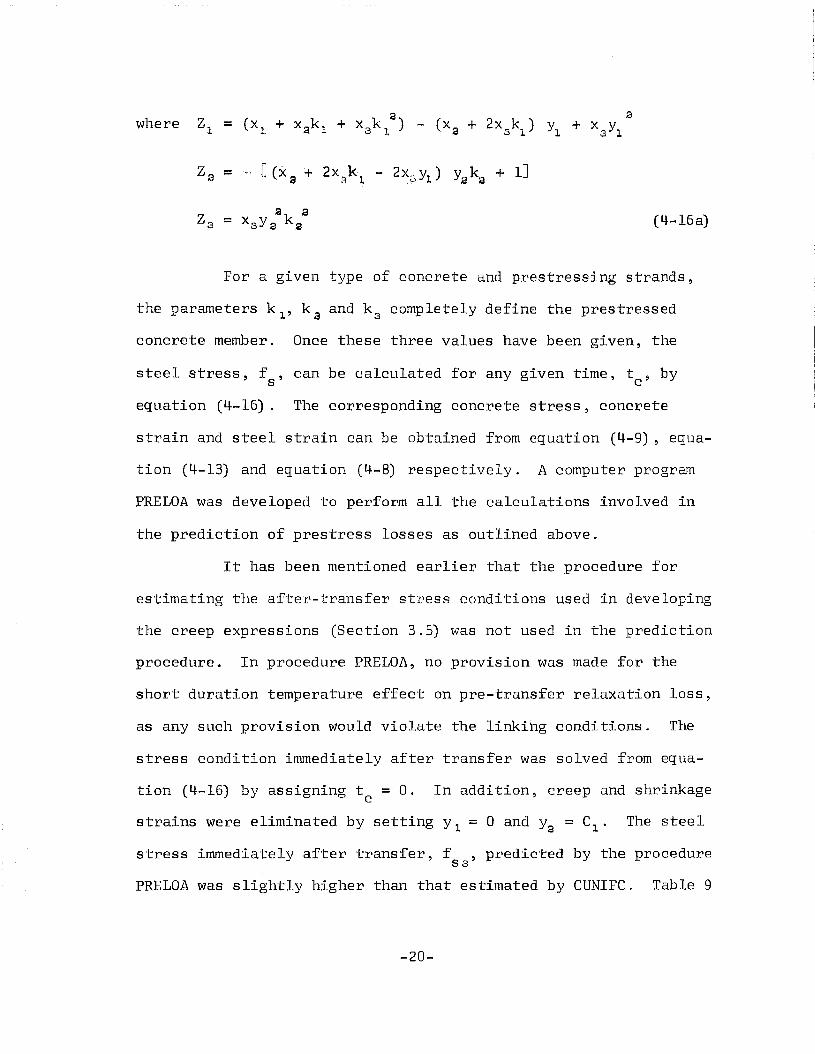
where Zl (Xl xa.k 1, +a

(X a 2xs kl

)a

= + xSk1

) - + Y1 + X aYl

Z:a = '" [ex a + '2x, k -. 2x;J Y1 ) Yaks + 1J3 l

2 3a a

= XsY.a k a (4-16a)

For a given type of concrete aQd prestressing strands,

the parameters k 1 , k s and k s completely define th~ prestressed

concrete member. Once these three values have been given, the

steel stress, f , can be calculated for any given time, t , bys c

equation (4-16). The corresponding concrete stress, concrete

strain and steel strain can be obtained from equation (4-9), equa-

tion (4-13) and equation (4-8) respectively. A computer program

PRELOA was developed to perform all the calculations involved in

the prediction of prestress losses as outlined above.

It has been mentioned earlier that the procedure for

estimating the after-transfer stress conditions used in developing

the creep expressions (Section 3.5) was not used in the prediction

procedure. In procedure PRELOA, no provision was made for the

short duration temperature effect on pre-transfer relaxation loss,

as any such provision would violate the linkihg conditions. The

stress condition immediately after transfer was solved from equa-

tion (4-16) by assigning t = O. In addition, creep and shrinkagec

strains were eliminated by setting Yl = 0 and Y2 = C1 • The steel

stress immediately after transfer, f predicted by the procedureS 3'

PRELOA was slightly higher than that estimated by CUNIFC. Table 9

-20-

exhibits a comparison for the ten series of uniformly prestressed

specimens. It is observed that the two sets of f values differS3

by only 2 to 3.5%, which is indeed tolerable.

It should be pointed out that equation (4-16) is appli-

cable only to uniformly (centrally) prestressed members subjected

to no external loading. For members nonuniformly (eccentrically)

prestressed, and/or subjected to external loading, the equilibrium

condition (4-9) would have to be generalized. However, the same

concept of combining the two stress-strain-time relationships

should be equally valid. Therefore, subject to further modifica-

tions and verifications, this general analytical procedure is ex-

pected to be applicable to any pretensioned prestressed concrete

member.

-21-

5. DISCUSSION OF RESULTS AND SUMMARY

5.1 Application of Prediction Method

As an initial test of feasibility of the prediction

method described in Chapter 4, the procedure was applied to the

ten series of uniformly stressed specimens. Based on the known

initial stress condition, geometrical design and the fabrication

schedule (k'~i",:>'" k a and k3), predicted prestress losses and concrete

strain at various times were calculated. Values of k1

, k and kg 3

as well as those of ~, the amount of '~:teel- reinforq~~:,ment, fo·~·"the

ten ~ 8e:~Iile~s';i-bf(j:-tinti':f-trf'mlystresse-d specimens are shown in Table 10.

The predicted prestress losses at various times for the

different s.e~ies· of specimens are listed in Table 11. The total

p~estress losses at 100 years, taken as the lifetime of a bridge

structure, varied from 33% to 47% of the initial prestress for

plant AB concrete and 24% to 37% for plant CD concrete. It should

be pointed out, however, that these high values of prestress loss

were due to the fact that the specimens were not externally

loaded. For actual structural members, externally applied dead

and live loads would reduce the concrete stress in the members

considerably, and lower percentage losses of prestress would be

typical.

-22-

5.2 Comparison of Predicted Results (PRELOA)

with Three-Dimensional Results (CUNIFB)

The predicted concrete strains were compared with the

results of the earlier three-dimensional analysis (CUNIFB). The

predicted concrete strains and the comparisons, in terms of per­

centage differences, at times 10, 100, 1000 and 36500 days are

shown in Tables 12, 13, 14 and 15 respectively.

In examining the tables, it should be borne in mind

that the entire analysis has been based on test data of the first

1000 days. The values in Table 15, for 100 years, were therefore

obtained through extrapolation and their accuracy cannot be

verified.

The comparisons showed that the results from the three­

dimensional analysis and the predicted results agree very well.

The maximum deviation is 12%. However, in most cases, the devia­

tions are about 5% or lesso

5.3 Effects of Types of Concrete and Initial Prestress

In Table 11 are shown prestress losses at various times

expressed as a fraction of the 100 year loss (taken as the ulti­

mate value). It can be observed that for the same initial pre­

stress level, the two concrete mixes showed approximately the

same prestress losses at any given time. In other words, the

type of concrete does not have any significant effect on the

growth of prestress loss. On the other hand, concrete from plant

-23-

CD consistently show~d lower prestress losses (absolute) than

concrete from plant AB. This was expected since concrete from

plant CD had lower loss characteristics than that from plant AB

(as was mentioned in Chapter 1) •

It can also be clearly observed that higher initial

prestresses yield higher prestress losses-

5.4 Summary

Two stress-strain-time relationships were developed sep­

arately for steel and concrete. These two relationships were then

integrated to form a combined TTconcrete-steelTT stress-strain-time

relationship, which~was applied on the different series of test

specimens to predict concrete strains and prestress losses. Com­

parison of these predicted results and the results from the three­

dimensional analysis showed that the developed prediction method

applied very well.

It was observed that the growth of prestress loss did

not depend on the type of concrete used, and that the higher the

initial prestress level the higher the prestress lasso

The validity of the proposed prediction method in this

report is yet to be justified by comparisons with the test data

of non-uniformly stressed specimens. This is logically the next

step to be taken in this project.

-24-

6 . ACKNOWLEDGMENTS

The study reported herein is a part of a research pro­

ject at the Fritz Engineering Laboratory, Lehigh University, under

the auspices of the Office of Research. The project is finan­

cially sponsored by the Pennsylvania Department of Transportation,

the U. S. Department of Transportation, Federal Highway

Administration;· and the Reinforced Concrete Research Council.

The help rendered by Mr. John Gera in tracing the

graphs, and that by Mrs. Ruth Grimes in typing the manuscript,

are gratefully acknowledged.

-25-

7. TABLES

-26-

TABLE 1: TWO-DIMENSIONAL RESULTS FOR

UNIFORMLY STRESSED SPECIMENS

Predicted* StandardPlant Series Strain Error

1.0 .1700 .0067

1.5 .1635 .0083

AB 2.0 .2132 .0059

3.0 .2398 .0071

3.6 .2440 .0083

1.0 .0917 .0037

1.5 .1156 .0047

CD 2.0 .1159 .0050

3.0 .1545 .0060

3.6 .1801 .0053

* Predicted strains at t = 36500 Days

-27-

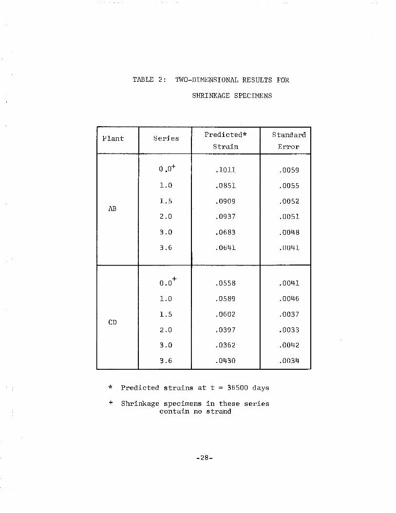
TABLE 2: TWO-DIMENSIONAL RESULTS FOR

SHRINKAGE SPECIMENS

Plant Series Predicte"d* Standard

Strain Error

o 0+ .1011 .0059' .1.0 .0851 .0055

1.5 .0909 .0052AB

2.0 .0937 .0051

3.0 .0683 .0048

3.6 .0641 .0041

0.0+ .0558 .0041

1.0 .0589 .0046

1.5 .0602 .0037CD

2.0 .0397 .0033

3.0 .0362 .0042

3.6 .0430 .0034

* Predicted strains at t = 36500 days

+ Shrinkage specimens in these seriescontain no strand

-28-

INlCI

TABLE 3: THREE-DIMENSIONAL RESULTS FOR UNIFORMLY STRESSED SPECIMENS

Plant Predicted Strain After 100 Years Standard

1.0* 1.5* 2.0* 3.0* 3.6* Error

AB .1630 .1798 .1966 .2301 .2502 .0084

CD .0928 .1087 .1245 .1562 .1752 .0057

AB-CD .1274- .1450 .1626 .1979 .2190 .0190

* Initial Nominal Concrete Stress in ksi, same as series name

TABLE 4: THREE-DIMENSIONAL RESULTS FOR SHRINKAGE SPECIMENS

Predicted Strain After 100 Years StandardPlant

0.0* 1.0* 1.5* 2.0* 3.0* 3.6* Error

AB .0995 .0914 .0873 .0832 .0750 .0701 .0059

CD .0677 .0585 .0539 .0494 .0402 .0347 .0050

AB-CD .0857 .0765 .0720 .0674 .0583 .0528 .0096

* Initial Nominal Concrete Stress in ksi, same as series name

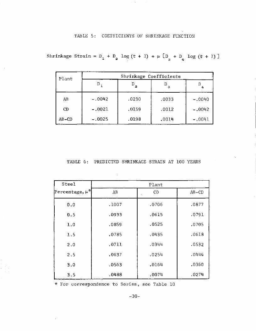
TABLE 5: COEFFICIENTS OF SHRINKAGE FUNCTION

Shrinkage Strain = Dl

+ Da log (t + 1) + I.l. [D3

+ D4

log (t + 1) ]

Plant Shrinkage Coefficients

D1 D D D;a 3 4

AB -.0042 .0230 .0033 -.0040

CD -.0021 .0159 .0012 -.0042

AB-CD -.0025 .0198 .0014 -.0041

TABLE 6: PREDICTED SHRINKAGE STRAIN AT 100 YEARS

Steel Plant

tpercentage,~* AB CD AB-CD

0.0 .1007 .0706 .0877

0.5 .0933 .0615 .0791

1.0 .0859 .0525 .0705

1.5 .0785 .0435 .0618

2.0 .0711 .0344 .0532

2.5 .0637 .0254 .0446

3.0 .0563 .0164 .0360

3.5 .0488 .0074 .0274

* For correspondence to Series, see Table 10

-30-

TABLE 7 COEFFICIENTS OF CREEP FUNCTION

Creep Strain = £1 + E~ log (t + 1) + f [E + E log.(t + 1) ]Ita C 3 4

Plant Creep Coefficients

£1 E E E2 3 4

AB -.0161 .0087 -.0018 .. 0185

CD -.0082 -.0023 -.0030 .0161

AB-CD -.0165 .0074- .0022 .0140

TABLE 8: PREDICTED CREEP STRAIN AT 100 YEARS

Constant PlantConcreteStress AB CD AB-CD

ksi

0.5 .0649 .0167 .0503

1.0 .1063 .0520 .0834-

1.5 .1476 .0873 .1165

2.0 .1890 .1226 .1496~

2.5 .2303 .1579 .1827

3.0 .2717 .1932 .2158

3.5 .3131 .2285 .2488

-31-

*

TABLE 9: COMPARISON OF f FOR CUNIFC* AND PRELOA'+S3

f f IfSeries Sl 83 pu

f CUNIFC PRELOApu

1.0 .6645 .6103 .6224

1·.5 .6968 .6293 .6414

~.6645

.f-I2.0 .5834- .6025

tjctl

r-I 3.0 .6968 .5954 .6130~

3.6 .6968 .5835 .6021

i]~;

1.0 .6645 .6212 .6273

1.5 .. 6968 .6384 .6480~u..I-J 2.0 .6645 .5981 .6105J::ctl

r-I~

3.0 .6968 .6087 .6236

3.6 .6968 .5922 .6141

CUNIFC - Creep Analysis (Section 3.4)(allowing temp. effect on pre-transfer relaxation)

+ PRELOA - Prediction Method (Section 4.4)(ignoring temp. effect on pre-transfer relaxation)

-32-

TABLE 10: VALUES OF 'k 1 , 'k2

, k3

AND ~ .

FOR VARIOUS SERIES OF SPECIMENS

'k 'k k I-L1 :3 3

Plant Series(.01 in/in) (days) (%)

1.0 .6393 0.00563 3.17 .65

1.5 .6721 0.00804 3.10 .89

AB 2.0 .6393 0.01130 3.10 1.21

3.0 ,6721 0.01622 3.04 1.70

3.6 .6721 0.01952 3.00 2.03

1.0 .6393 0.00563 2.19 .65

1.5 .6721 0.00804 2.17 .89

CD 2.0 .6393 O.Ovl130 2.00 1.21

3.0 .6721 0.01622 1.96 1.70

3.6 .6721 0.01952 1.92 2.03

-33-

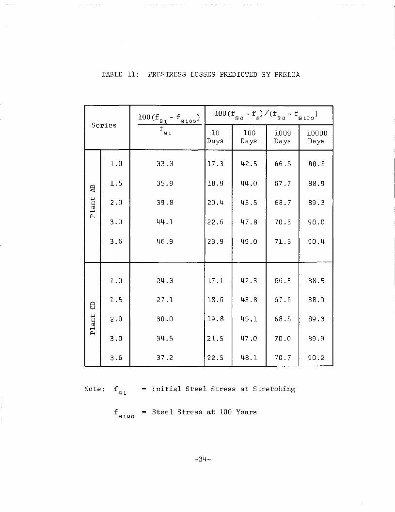
TABLE 11: PRESTRESS LOSSES PREDICTED BY PRELOA

100(£ - fS lOO)

100(f -f)/(f -f )s 3 S S 3 S 100

Series81

f81 10 100 1000 10000

Days Days Days Days

1.0 33.3 17.3 42.5 66.5 88.5

~1.5 35.9 18.9 44.0 67.7 88.9

4-J2.0 39.8 20.4 45.5 68.7 89.3~

cor-IiJ..4

3.0 44.1 22.6 47.8 70.3 90.0

3.6 46.9 23.9 49.0 71.3 90.4

1.0 24.3 17.1 42.3 66.5 88.5

1.5 27.1 18.6 43.8 67.6 88.9Qu..J-J 2.0 30.0 19.8 45.1 68.5 89.3c::ro

r--IP4

3.0 34.5 21.5 47.0 70.0 89.9

3.6 37.2 22.5 48.1 70.7 90.2

Note: fS1

= Initial Steel Stress at Stretching

f = Steel Stress at 100 Years8100

-34-

TABLE 12: PREDICTED CONCRETE STRAINS AT 10 DAYS

Concrete Strain 100 (CUNIFB-PRELOA)SeriesCDNIFB* PRELOA+ CUNIFB

1.0 .0304- .0266 12.5

1 .. 5 .0346 .0329 4.9

~4-J 2.0 .0389 .0385 1.0c:C'd

r-I~

3.0 .0475 .0488 2.7

3'.6 .0526 .0541 2.9

1.0 .0149 .0138 7.4-

1.5 .0185 .0184 0.5~u.J-I

2.0 .0220 .0226 3.0cro

r-I~

3.0 .0291 .0305 4.8

3.6 .0334 .0347 3.9

* CUNIFB - Results of Three-Dimensional Analysis

+ PRELOA - Predicted Results

-35-

TABLE 13: PREDICTED CONCRETE STRAINS AT 100 DAYS

Concrete Strain100 (CUNIFB-PRELOA)Series

CUNIFB* PRELOA+ CUNIFB

1.0 .0667 .0665 0.3

1.5 .0743 .0770 3.6

~+..J 2.0 .0820 .0856 4.8c:cd

r--i~

3.0 .0974 .1019 4.6

3.6 .1066 .1097 2,.9

1.0 .0362 .0362 0.0

1.5 .0432 .04-51 4.4~u+..J

2.0 .0501 .0527 5.2ccd

r--i~

3.0 .0639 .0673 5.3

3.6 .0722 .0747 3.5

*+

CUNIFB - Results of Three-Dimensional Analysis

PRELOA - Predicted Results

-36-

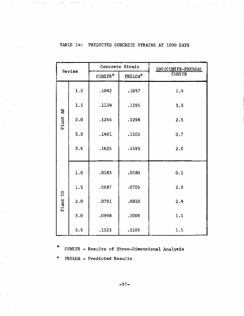
TABLE 1.... : PREDICTED CONCRETE STRAINS AT 1000 DAYS

Cencrete Strain 100 (CUNIFB-PRELOA)SeriesCUNIFB* PRELOA+ CUNIFB

1.0 .1042 .1057 1.4

1.5 .1154 .1195 3.5~4-J 2.0 .1266 .1298 2.5a,....ftJ..

3.0 .1491 .1502 0.7

3.6 .1625 .1593 2.0

1.0 .0583 .0580 0.5

1.5 .0687 .0706 2.8Qu..... 2.0 .0791 .0810 2.4Qro

....-4P-I

3.0 .0998 .1009 1.1

3.6 .1123 .1106 1.5

* CUNIFB - Results of Three-Dimensi.onal Analysis

+ PRELOA - Predicted Results

-37-

TABLE IS: PREDICTED CONCRETE STRAINS AT 100 YEARS

-Concrete Strain 100 (CUNIFB-PRELOA)Series

CUNIFB* PRELOA+ CUNIFB

1.0 .1630 .1635 0.3

1.5 .1798 .1808 0.6IXl<.J.J 2.0 .1966 .1919 2.1c:res~

P-4

3.0 .2301 .2156 6.3

3.6 .2502 .2249 10.1

1.0 .0928 .0901 2.9

1.5 .1087 .1073 1.3

e~ 2.0 .1245 .1209 2.9t:nt~

P-4

3.0 .1562 .1467 6.1

3.6 .1752 .1586 9.5

* CUNIFB ~ Results of Three-Dimensional Analysis

+ PRELOA - Predicted Results

-38-

8. FIGURES

-39-

-...---..1.5 2.0

SERIES 1.01.0

0.0

1.0

SERIES 1.5

1.5

0.0

14-7/16" STRANDS0.5

20 - ~16u STRANDS

1.0

F, =20.6 k/STRAND

0.0

Fj = 21.6 k/STRAND

0.0

"""----.. 3.0

SERIES 2.0 28 - 7/1611

STRANDS

2.0 1.0

0.0

""'-----... :3.0

Fj =20.6 k/STRAND

0.4

'------.... 3.6

SERIES 3.0 40- ~16" STRANDS Fj =21.6 k/STRAND

p------.... 3.0

0.0

"""----.... :3 .0

SERIES 3.6 48- 7/IS1

STRANDS Fj = 21.6 k/STRAND....----.....-.... :3 .6

0.0

........----.... 3.6

• No. Inside of Fig. Represent I e I

• No. Outside of Fig. Represent InitialNominal Stress

• All Strands Are 270k VIS1

ep 7 WireUncoated Stress Rei ieved

Fig. 1 Stress Distributions for Rectangular Specimens

-40-

0.25c~c-q0

- 0.20z-<Xc:::~CJ)

w 0.15~w0:::U

I Z+= 0f-l u 0.10I

~ZW0ZW0- 0.05w0

I

W~-~

10 100 1000TIME IN DAYS

3.6

3.0

2.0

1.5

1.0

10000 36500

Fig. 2 Time-Dependent Concrete Strain VB. Time for Plant AB

c::~ 0.20c-00 ~ ____ 3.6

-ZI ~ ~3.0-« 0.15

0:::~en r ~ ~ ~2.0W~ I ~ ~ ~ ______ I •5w0::: 0.10u I ~~ ~ ~ ~I.O

I Z-1= 0N UI

I-z 0.05w0zwa..w0

I -I 10 100 1000 10000w 36500~ TIME IN DAYS~

Fig. 3 Time-Dependent Concrete Strain vs. Time for Plant CD

10000 36500100 1000TIME IN DAYS

100

1

0.10I

3.6

c:: I /~3.0

" - / 2.0.s: 0.080

l ~/,:~~0...z-<{

~ 0.06en

w(!)

Ic:::(

.;= ~UJ z 0.04I -

a::Ien

0.02

Fig. 4 Shrinkage Strain vs. Time for Plant AB

<D q 0 to 0 0rO ,." C\J

./ 0- - L(')tort'>

0000

QCJ

~

0§

r-I

0 ~

0 (J) ~

>- 0

<t ~

0 OJE

Z-,-IE-I

W rn

:2i:>

0 - J::~

-,-I

0 cd~~enOJbOcd

.-a-,-I~

r.c:UJ

0 tJ1

.bO

eMI:J-I

rooo

lDoo

q­qo

C\Joo

o

-44-

9~ REFERENCES

1. Rokhsar, A. and Huang, T.COMPARATIVE STUDY OF, SEVERAL CONCRETES REGARDING THEIRPOTENTIALS FOR CONTRIBUTING TO PRESTRESS LOSSES, FritzEngineering Laboratory Report No. 339.1, LehighUniversity, May, 1968.

2. Huang, T. and Frederickson, D. C.CONCRETE STRAINS IN PRE-TENSIONED CONCRETE STRUCTURALMEMBERS - PRELIMINARY REPORT, Fritz Engineering Labora­tory Report No. 339.3, Lehigh University, July, 1969.

3. Schultchen, E., Ying, H. and Huang, T.RELAXATION BEHAVIOR OF PRESTRESSING STRANDS, FritzEngineering Laboratory Report No. 339.6, LehighUniversity, March, 1972.

-45-

APPENDIX

NOTATIONS

All 'notations have been defined when they first appeared

in this report. They are assembled here for easy reference. Un-

less specifically indicated otherwise, all quantities are in con-

sistent inch-kip-day units. All strain quantities are in 0.01

in./in.

Ac = Area of net concrete cross section (gross section area sub­

tract the area of prestressing steel)

Aps = Area of prestressing steel

E = Secant modulus of elasticity of concretec

f = Stress in concretec

f. = Initial concrete nominal stress (used in CUNIFC)1

f = Ultimate tensile strength of steelpu

f = Stress in steels

k 1 = Initial strain of steel at tensioning, in 0.01 in./in.

k a = Ratio of A to Ac' dimensionlessps

k a = Time interval from initial tensioning to transfer

L = Loss of steel stress due to relaxation

Sa = Concrete strain

-46-

s = Creep st~ain of concretecr

S = Total measured concrete strainct

Sel = Elastic strain of concrete

S = Elastic rebound strain of concreteer

S = Steel strains

8sh = Shrinkage strain of concrete

t = "Concrete time", starting from transferc

t = "Steel time TT, starting' -from···tensioning

s

~ = Amount of longitudinal steel, both prestressed and non-

prestressed, in percent of gross Section area

Numerical subscripts used with stress notations to desig-

nate time:

1 Time of initial tensional

2 Immediately before transfer

3 Immediately after transfer

-47-