estimation for counting processes with high-dimensional
TRANSCRIPT
HAL Id: tel-01119228https://tel.archives-ouvertes.fr/tel-01119228
Submitted on 22 Feb 2015
HAL is a multi-disciplinary open accessarchive for the deposit and dissemination of sci-entific research documents, whether they are pub-lished or not. The documents may come fromteaching and research institutions in France orabroad, or from public or private research centers.
L’archive ouverte pluridisciplinaire HAL, estdestinée au dépôt et à la diffusion de documentsscientifiques de niveau recherche, publiés ou non,émanant des établissements d’enseignement et derecherche français ou étrangers, des laboratoirespublics ou privés.
Estimation for counting processes with high-dimensionalcovariatesSarah Lemler
To cite this version:Sarah Lemler. Estimation for counting processes with high-dimensional covariates. Statistics [stat].Universite d’Evry Val d’Essonne, 2014. English. tel-01119228

Université d’Évry Val d’EssonneLaboratoire de Mathématiques et Modélisation d’ÉvryÉcole doctorale 423 : des Génomes Aux Organismes
Thèse
présentée en première version en vue d’obtenir le grade de
Docteur de l’Université d’Évry Val d’Essonne
Spécialité : Mathématiques
par
Sarah Lemler
Estimation for counting processes
with high-dimensional covariates
Thèse soutenue le 9 décembre 2014 devant le jury composé de :
Fabienne COMTE Université Paris Descartes (Examinatrice)Jean-Yves DAUXOIS Université de Toulouse (Examinateur)Cécile DUROT Université Paris Ouest Nanterre la Défense (Rapporteure)Agathe GUILLOUX Université Pierre et Marie Curie (Directrice)Sylvie HUET INRA unité MIAGE (Examinatrice)Sophie LAMBERT-LACROIX Université de Grenoble (Rapporteure)Marie-Luce TAUPIN Université d’Évry Val d’Essonne (Directrice)

Laboratoire de Mathématiques et Modélisation d’Évry(LaMME)Université d’Évry Val d’Essonne (UEVE)Institut de Biologie Génétique et BioInformatique (IBGBI)4ème étage23 boulevard de France, 91 037 Évry
Laboratoire de Statistique Théorique et Appliquée (LSTA)Université Pierre & Marie Curie (UPMC)Tour 25, couloirs 15-25 & 15-162ème étage4, place Jussieu, 75252 Paris Cedex 05

À mes parents


Remerciements
Ces quelques lignes, sans doute trop courtes, pour remercier toutes les personnes quim’ont permis de mener à bien cette aventure.
Mes premiers remerciements vont à mes deux directrices de thèse Agathe et Marie-Luce.J’ai pu mesurer au cours de ces trois ans et demi la chance que j’ai de vous avoir pour di-rectrices de thèse et ces quelques lignes ne suffiront pas à vous exprimer toute ma gratitude.Marie-Luce, c’est d’abord à toi que je dois d’être là. Merci de m’avoir fait découvrir l’analysede survie, un champ des mathématiques dont j’ignorais l’existence et dont les applications àla médecine m’ont convaincue de l’importance de la recherche théorique en mathématiquesdans un domaine si essentiel. Merci surtout d’avoir cru en moi et de m’avoir dit cette seulephrase « si tu cherches un stage de M2 ou une thèse n’hésite pas à me contacter », qui amodifié mon parcours et m’a propulsée dans une sphère que je n’aurais jamais envisagé êtreen mesure de rejoindre. Je tiens aussi à te remercier pour ta réactivité à mes sollicitations,ta patience et ton soutien dans les moments de doute. Agathe, merci d’avoir suivi de siprès tout mon travail pendant ces trois ans et demi et d’avoir partagé avec moi ta grandeculture scientifique. Merci pour ta grande disponibilité, ta patience et tes encouragements.Je te remercie aussi de m’avoir poussée à programmer en R alors même que je faisais toutpour reculer le moment de m’y mettre et de m’avoir ainsi prouvé que j’en étais capable.J’espère un jour avoir ta rapidité à comprendre un problème et à trouver une solution pourle résoudre. Merci à toutes les deux pour la confiance que vous m’avez témoignée et surtout,pour tout le temps que vous m’avez consacré tout au long de ma thèse et particulièrementces derniers mois de rédaction (parfois même jusqu’à 22h un vendredi ou un samedi soir pourme rassurer sur mes doutes ou répondre à mes questions). À toutes les deux, un immensemerci et j’espère que notre histoire continuera (avec moins de sollicitations, c’est promis) !
Merci à mes deux rapporteures, Cécile Durot et Sophie Lambert-Lacroix, pour m’avoirfait l’honneur de rapporter ma thèse. Je vous remercie sincèrement toutes les deux pourle temps que vous avez consacré à mon travail et pour les commentaires enrichissants etprécieux pour la suite. Cécile Durot, je tiens à vous exprimer toute ma gratitude pour larelecture si attentive et minutieuse que vous avez faite de ma thèse et pour m’avoir ainsipermis d’améliorer mon travail grâce à vos remarques pertinentes et à vos conseils. SophieLambert-Lacroix, merci pour votre relecture bienveillante et circonstanciée.
Merci à Fabienne Comte, Sylvie Huet et Jean-Yves Dauxois d’avoir si aimablement etrapidement accepté de faire partie de mon jury de thèse. Merci Fabienne pour m’avoir faitdécouvrir les statistiques non-paramétriques en Master 2 et surtout pour l’intérêt que vousavez continué à porter à mon travail pendant ma thèse. Merci pour toutes les fois où vousavez pris le temps de répondre à mes sollicitations et merci aussi de m’avoir conseillée lorsquej’avais des doutes. Sylvie, merci d’avoir suivi mon travail pendant ces trois ans et demi, àl’occasion d’un séminaire SSB, de mon comité de thèse ou d’un exposé à Fréjus. Merci pour

votre regard éclairant et bienveillant sur mon travail. Merci Jean-Yves d’avoir été le premier àaccepter de faire partie de ce jury. Je suis ravie d’avoir fait votre connaissance à cette occasion.
Je tiens à remercier tous les membres de l’équipe Statistique et Génome. Quand je suisarrivée au laboratoire pour mon stage de Master 2, j’y ai été extrêmement bien accueillie,et si pendant ces trois années de thèse, je m’y suis sentie aussi bien, vous y êtes tous pourbeaucoup. Merci Cyril, j’ai eu plaisir à partager avec toi les TDs de L2 bio pendant ces quatreannées. Je te remercie aussi pour ton oreille attentive, tes conseils et pour m’avoir remontéle moral quand j’en ai eu besoin. Merci Maurice pour avoir tant de fois partagé mes plainteslorsque le RER D faisait des siennes et égayé mes trajets à force de bons plans à Paris, dediscussions sur les films, les livres, les expositions, les applications... Merci Catherine pourtes conseils, pour avoir toujours pris le temps de répondre à mes questions et pour m’avoirfait découvrir de grands chorégraphes contemporains ! Merci Carène pour ta bonne humeuret tes petites attentions qui font toujours plaisir, merci Yolande pour ton rire communicatifet vive la zumba ! Claudine, si tu n’existais pas il faudrait t’inventer, alors merci de mettreautant d’ambiance au labo ! Merci Michèle pour ton accueil si chaleureux à mon arrivéeau laboratoire, pour cette journée au Château de Fontainebleau et à Barbizan et pour lesnombreuses discussions. Merci aussi à Anne-Sophie pour ton cours sur le modèle linéaire etsurtout pour tes encouragements dans les moments difficiles, à Bernard pour m’avoir aussibien préparée à l’audition pour obtenir ma bourse de thèse, à Christophe pour toujours avoirfait en sorte que je puisse participer à toutes les conférences qui m’intéressaient, à Pierre pourton calme à toute épreuve qui fait du bien, à Julien en souvenir des TDs de L1 pendant mapremière année et à Guillem. Merci Valérie pour ton aide pour l’organisation de la soutenance.Merci à Camille et Marine pour avoir guidé mes pas dans le monde des doctorants. Marius,mon grand frère de thèse, merci de m’avoir supportée pendant ces trois années et demi,merci pour les nombreuses discussions de mathématiques et autres et pour ton soutien sansfaille, merci aussi à Van Hanh pour son sourire si communicatif. Merci à Alia vive Maths EnJeans, Edith pour nos nombreuses discussions autour de la gym suédoise, la zumba ou touteautre chose, Margot pour tes encouragements et nos discussions pendant les trajets de RER,Morgane pour nos nombreuses discussions dans la cuisine, dans les couloirs ou dans le RER,merci pour toutes ces pauses bavardages qui font du bien, Virginie ma nouvelle co-bureauet compagnonne de Zumba, merci de m’avoir fait découvrir les codes RGB qui ouvrent unchamp des possibles infini sur beamer, Jean-Michel pour toutes les fois où tu as voulu mefaire sursauter de peur et où tu as échoué, mais aussi pour toutes les discussions à propos demaths ou pas, Benjamin que j’ai eu plaisir à retrouver au laboratoire deux ans après notreMaster 2 et Quentin, merci à vous tous pour cette bonne entente !
Merci également à tous les thésards de Paris 6 et en particulier à mes compagnons debureau Assia, Roxane, Baptiste et Matthieu ainsi qu’à Cécile, Benjamin, Erwan et Mokhtarpour m’avoir si gentiment intégrée à leur petite équipe !
Merci à Adeline Samson pour m’avoir si bien dirigée vers Marie-Luce lorsque je l’aicontactée pour mon stage de Magistère. Un grand merci également à Patricia Reynaud-Bouret et Franck Picard pour l’intérêt qu’ils m’ont porté au colloque Jeunes Probabilisteset Statisticiens à Forges-les-Eaux. Merci à tous les deux pour tous vos conseils et encourage-ments. Merci Patricia pour tes suggestions éclairantes sur mon travail.
Merci à tous les jeunes statisticiens que j’ai croisés pendant ces trois années. Gaëlle, jesuis ravie d’avoir fait ta connaissance à Fréjus juste avant de commencer ma thèse, merci de
vi

m’avoir aidée à comprendre comment faire mes voeux inter-académiques, merci de toujoursrépondre à mes questions de manière détaillée et claire, enfin, ta thèse, si bien rédigée m’abien aidée à comprendre la méthode de Goldenshluger et Lepski. Merci aussi à Angelina età tous mes compères de Saint-Flour avec qui j’ai vraiment passé de bons moments : Carole,Laure, Lucie, Ilaria, Mélisande, Andrés, Benjamin, Clément et Sébastien.
Je tiens à présent à remercier mes amis pour tous ces bons moments partagés au quo-tidien, en week end, en vacances ou lors de notre BNH annuel. Tout d’abord mes deuxinconditionnels soutiens, Flo et Marion, merci d’être toujours là dans les bons moments,mais aussi dans les moments plus difficiles. Merci à vous deux de m’avoir soutenue pendantla période de rédaction, motivée avec vos messages et de ne jamais m’avoir reproché de nepas avoir de temps pour vous pendant toute cette période. Merci surtout à chacune d’entrevous pour les innombrables bons moments partagés et nos interminables discussions ! Merciaussi à Marion pour toutes ces années d’amitié depuis le primaire et pour tes mails pleind’attention tout au long de la rédaction. Emilie, merci pour ta générosité, pour les soiréesjeux et toutes nos discussions sur nos thèses, mais pas seulement, loin sans faut. Jo, mercide prendre toujours régulièrement de mes nouvelles et de toujours me remotiver dans mesmoments de doute avec des smileys d’encouragement, toi qui sais si bien ce que c’est que defaire une thèse. Je remercie également Eleo (pour nos longues conversations téléphoniquesmoins fréquentes qu’au lycée, mais avec toujours autant de choses à se dire), Pauline, Alix,Laure (pour toutes tes invitations si conviviales pour tes anniversaires ou les fêtes), Alex,Hugo, Pierre, Vincent, Guillaume, Louis-Marie. Merci enfin à Laura, mon amie d’enfancequi, même si elle est loin, reste toujours présente.
Mes derniers remerciements et non les moindres vont à ma famille. Merci d’abord à mesgrands-parents qui ont toujours été fiers de leurs petits-enfants et qui ne s’en sont jamaiscachés : merci de croire autant en moi. Léna, ma sis’, quelle chance précieuse j’ai que tu soislà ! Je ne pourrai jamais assez te dire à quel point ton soutien compte pour moi. Merci pourtoutes tes attentions, pour les ondes positives que tu m’envoies régulièrement et pour bienplus encore ! Surtout, merci pour tous nos bons moments à deux. Enfin, mes plus profondsremerciements sont pour vous Maman et Papa. Ma reconnaissance pour tout ce que vousm’apportez va bien au-delà de ces quelques lignes et je ne saurais exprimer tout ce que je vousdois. En voici donc une infime partie. Je vous remercie tous les deux pour votre inébranlablesoutien en toute épreuve et vos conseils avisés. Merci de m’avoir toujours soutenue dans meschoix, de m’avoir poussée à toujours viser plus loin, plus haut, merci de la confiance que vousavez en ma réussite. Merci aussi à tous les deux d’avoir pris le temps de relire les parties enfrançais de ma thèse pour corriger les fautes d’orthographe. Maman, merci pour tout le tempsque tu me consacres (heureusement que les forfaits téléphoniques sont illimités !), merci detoujours me simplifier les aspects matériels, merci pour tous les bons petits plats que tu meprépares pour ma semaine lorsque je rentre pour le week end, merci de prendre autant soinde moi. Papa, je me rappelle lorsque tu me faisais faire des « problèmes » au primaire et quetu m’as initiée aux logigrammes, je détestais ça et rien ne laissait alors présager que j’allaisfaire des maths plus tard ! Merci de pouvoir toujours aussi compter sur toi, merci pour tesconseils et merci surtout de me prouver très souvent qu’il faut que j’aie plus confiance enmoi ! Merci pour cette chance inestimable que vous m’offrez, tous les deux, de pouvoir autantcompter sur vous !
vii


Organisation de la thèse
Cette thèse est consacrée à l’estimation de la fonction de risque d’un processus decomptage, en présence d’un vecteur de covariables de grande dimension. Nous propo-sons différentes procédures d’estimation. Pour chacun des estimateurs obtenus, nousétablissons des inégalités oracles non-asymptotiques assurant leurs performances théo-riques. Enfin, une implémentation pratique des différentes procédures est proposée.Cette thèse comporte quatre chapitres (hors introduction) répartis en deux parties.
— Le Chapitre 1 est une introduction générale : nous y présentons le contexte,une description des méthodes d’estimation utilisées, les démarches de preuves etenfin nos contributions. Les méthodes d’estimation et les démarches de preuvessont dans un premier temps, décrites dans des modèles plus simples, le modèlede régression additive et le modèle d’estimation de densité, en mettant en évi-dence les similitudes et différence entre les méthodes. Puis nous expliquons notrecheminement dans ce travail et nos contributions dans chacune des deux partiesde la thèse.
— La Partie I est consacrée à l’estimation non-paramétrique de l’intensité d’unprocessus de comptage, en présence d’un vecteur de covariables en grande di-mension. Cette partie est constituée du Chapitre 2, suivie d’une annexe.
— Dans le Chapitre 2, nous proposons d’estimer l’intensité par un estima-teur de l’intensité dans un modèle de Cox, choisi automatiquement à partirdes données. Cette estimation est basée sur une procédure Lasso appliquéesimultanément aux deux fonctions intervenant dans le modèle de Cox : lerisque de base et le risque relatif. En annexe, nous faisons une présenta-tion mettant en perspective les similitudes et les différences entre l’étudedu Lasso en régression additive et l’étude du Lasso dans notre modèle deprocessus de comptage.
— La Partie II est consacrée à l’estimation de la fonction du risque de base dansle modèle de Cox, en présence d’un vecteur de covariables en grande dimension.Cette partie est constituée d’une introduction commune et de trois chapitres.Dans cette partie, nous proposons deux procédures d’estimation du risque debase, établissons des inégalités oracles non asymptotiques, et enfin procédons àune comparaison pratique des deux procédures d’estimation.
— L’Introduction, qui est commune aux Chapitres 3, 4 et 5, présente lecadre de travail commun à chacun de ces chapitres.

— Dans le Chapitre 3, nous proposons d’estimer le risque de base avec uneprocédure de sélection de modèles.
— Dans le Chapitre 4, nous proposons d’estimer le risque de base en utilisantun estimateur à noyau dont le paramètre de lissage est choisi de façonadaptative par la méthode de Goldenshluger et Lepski.
— Enfin, au Chapitre 5 nous menons une étude par simulations. Cette étudeprésente une comparaison des performances pratiques des procédures d’es-timation du risque de base proposées aux deux chapitres précédents. Nousterminons cette étude, en appliquant ces procédures d’estimation à un jeude données réelles sur le cancer du sein.
Nous avons aussi comparé les méthodes de sélection de modèles et de sélection defenêtres dans notre modèle, ainsi que les résultats obtenus pour ces estimateursaux Chapitres 3 et 4.
Chaque chapitre est précédé d’un court résumé permettant de le situer dans soncontexte.
x
Table des matières
Remerciements . . . . . . . . . . . . . . . . . . . . . . . . . . . . . . . . . . vOrganisation de la thèse . . . . . . . . . . . . . . . . . . . . . . . . . . . . . ix
Table des matières xi
Liste des figures xiii
Liste des tableaux xiv
1 Introduction 11.1 Cadre de travail . . . . . . . . . . . . . . . . . . . . . . . . . . . . . . . 21.2 Généralités sur les méthodes d’estimation et les résultats attendus . . . 111.3 Cheminement et principaux résultats . . . . . . . . . . . . . . . . . . . 32
I Estimation of the non-parametric intensity of a countingprocess by a Cox model with high-dimensional covariates 49
2 High-dimensional estimation of counting process intensities 512.1 Introduction . . . . . . . . . . . . . . . . . . . . . . . . . . . . . . . . . 532.2 Estimation procedure . . . . . . . . . . . . . . . . . . . . . . . . . . . . 562.3 Oracle inequalities for the Cox model for a known baseline function . . 602.4 Oracle inequalities for general intensity . . . . . . . . . . . . . . . . . . 652.5 An empirical Bernstein’s inequality . . . . . . . . . . . . . . . . . . . . 682.6 Technical results . . . . . . . . . . . . . . . . . . . . . . . . . . . . . . 712.7 Proofs . . . . . . . . . . . . . . . . . . . . . . . . . . . . . . . . . . . . 73Appendices . . . . . . . . . . . . . . . . . . . . . . . . . . . . . . . . . . . . 84A Connection between the weighted norm and the Kullback divergence . . 84B An other empirical Bernstein’s inequality . . . . . . . . . . . . . . . . . 87C Weighted Lasso procedure in the specific case of the Cox model . . . . 92D Detailed comparison with the additive regression model . . . . . . . . . 97
II Estimation of the baseline function in the Cox modelwith high-dimensional covariates 105
Introduction 107
xi

3 Adaptive estimation of the baseline hazard function in the Coxmodel by model selection 1133.1 Introduction . . . . . . . . . . . . . . . . . . . . . . . . . . . . . . . . . 1153.2 Estimation procedure . . . . . . . . . . . . . . . . . . . . . . . . . . . . 1163.3 Non-asymptotic oracle inequalities . . . . . . . . . . . . . . . . . . . . . 1233.4 Proofs . . . . . . . . . . . . . . . . . . . . . . . . . . . . . . . . . . . . 125Appendices . . . . . . . . . . . . . . . . . . . . . . . . . . . . . . . . . . . . 144A Prediction result on the Lasso estimator β of β0 for unbounded counting
processes . . . . . . . . . . . . . . . . . . . . . . . . . . . . . . . . . . . 144
4 Adaptive kernel estimation of the baseline function in the Cox model1474.1 Introduction . . . . . . . . . . . . . . . . . . . . . . . . . . . . . . . . . 1494.2 Estimation procedure . . . . . . . . . . . . . . . . . . . . . . . . . . . . 1504.3 Non-asymptotic bounds for kernel estimators . . . . . . . . . . . . . . . 1554.4 Proofs . . . . . . . . . . . . . . . . . . . . . . . . . . . . . . . . . . . . 158Appendices . . . . . . . . . . . . . . . . . . . . . . . . . . . . . . . . . . . . 172A Technical lemma . . . . . . . . . . . . . . . . . . . . . . . . . . . . . . 172B Unbounded case . . . . . . . . . . . . . . . . . . . . . . . . . . . . . . . 173
5 Simulations 1795.1 Simulated data . . . . . . . . . . . . . . . . . . . . . . . . . . . . . . . 1815.2 Step 1: Estimation of the regression parameter β0 . . . . . . . . . . . . 1845.3 Step 2: Estimation of the baseline function α0 . . . . . . . . . . . . . . 1875.4 Measuring the quality of the estimators . . . . . . . . . . . . . . . . . . 1935.5 Results in the case of simulated data . . . . . . . . . . . . . . . . . . . 1945.6 Application to a real dataset on breast cancer . . . . . . . . . . . . . . 205Appendices . . . . . . . . . . . . . . . . . . . . . . . . . . . . . . . . . . . . 210A The rectangle method . . . . . . . . . . . . . . . . . . . . . . . . . . . 210B Calibration of the constants . . . . . . . . . . . . . . . . . . . . . . . . 210C Description of the real data . . . . . . . . . . . . . . . . . . . . . . . . 212
Conclusion 215
A Appendices 219A.1 Un peu de théorie sur les processus de comptage . . . . . . . . . . . . . 220A.2 Construction de la vraisemblance de Cox . . . . . . . . . . . . . . . . . 224A.3 Quelques inégalités de concentration . . . . . . . . . . . . . . . . . . . 227
Bibliographie 229
xii

Liste des figures
1.1 Courbes des fonctions de risque d’un individu pris dans les conditions standardet d’un individu ayant des prédispositions génétiques. . . . . . . . . . . . . . 4
1.2 Illustration de la pénalisation ℓ1 . . . . . . . . . . . . . . . . . . . . . . . . . 131.3 Courbes du vrai risque de base (en rouge), de l’estimateur à noyau obtenu
par validation croisée (en vert), de l’estimateur par minimum de contrastepénalisé (en bleu) et de l’estimateur à noyau adaptatif (en noir). Les courbesont été obtenues pour : n = 500, p = ⌊√n⌋, α0 ∼ lnN (1/4, 0), 20% de censure 47
1.0.1 Plots of the baseline hazard function for different parameters of a log-normaldistribution (left) and of a Weibull distribution (right). . . . . . . . . . . . . 183
5.1.1 Median, first and third quartiles of |β − β0|1 (on the left) and for |β − β0|2(on the right), β being either β
ML, either β
Lassoor β
AdapL. . . . . . . . . . 196
5.2.1 Plots of the true baseline function (in red), the cross-validated kernel estimator(in green), the penalized contrast estimator (in blue) and the adaptive kernelestimator (in black). The plots have been obtain for: n = 500, p = ⌊√n⌋,α0 ∼ lnN (1/4, 0), d = 4.5 . . . . . . . . . . . . . . . . . . . . . . . . . . . . . 199
5.2.2 Median, first and third quartiles of the random MISEs of the kernel estimatorwith a bandwidth selected by cross-validation (5.2.2a), of the kernel estimatorwith a bandwidth selected by the Goldenshluger and Lepski method (5.2.2b),of the penalized contrast estimator in the case of histograms (5.2.2c) and ofthe penalized contrast estimator in the trigonometric case (5.2.2d), with theadaptive Lasso estimator of the regression parameter in the case of a Weibulldistribution W(1.5, 1). . . . . . . . . . . . . . . . . . . . . . . . . . . . . . . . 200
6.2.1 Kernel estimators with a bandwidth selected either by cross-validation (ingreen) or by the Goldenshluger and Lepski method (in black) and by modelselection estimator in the histogram basis (in blue). The first column is asso-ciated to the group of untreated patients and the second column correspondsto the group of Tamoxifen patients for p = 10 (first line), p = 100 (secondline) and p = 1000 (third line). . . . . . . . . . . . . . . . . . . . . . . . . . . 207
6.2.2 Kernel estimator with a bandwidth selected either by cross-validation (ingreen) or by the Goldenshluger and Lepski method (in black) and modelselection estimator in the trigonometric basis (in blue). The first column isassociated to the group of untreated patients and the second column corres-ponds to the group of Tamoxifen patients for p = 10 (first line), p = 100(second line) and p = 1000 (third line). . . . . . . . . . . . . . . . . . . . . . 208
xiii

Liste des tableaux
1.1 Tableau comparatif pour la procédure Lasso dans le modèle de régressionadditif et dans le modèle à intensité multiplicative d’Aalen non-paramétrique. 37
1.2 Tableau comparatif des méthodes de sélection de modèles et de Goldenshlugeret Lepski pour l’estimation du risque de base α0 en grande dimension. . . . . 43
5.1.1 ℓ1-norm and ℓ2 norm of estimation errors of the estimators βML
, βLasso
and
βAdapL
for n = 200 and p = 5, 15, 200, and n = 500 and p = 5, 22, 500. . . . . 195
5.1.2 ℓ1-norm and ℓ2 norm of prediction errors of the estimators βML
, βLasso
and
βAdapL
for n = 200 and p = 5, 15, 200, and n = 500 and p = 5, 22, 500. . . . . 1975.1.3 Specificities (SPEC) and sensitivities (SENS) for the Lasso and the adaptive
Lasso (AdapL) for n = 200 and p = 200. . . . . . . . . . . . . . . . . . . . . . 1985.1.4 ℓ1-norm of the estimation errors on the support of β0 and its complementary
for the maximum Cox partial likelihood and the Lasso estimators for n = 200and p = 15. . . . . . . . . . . . . . . . . . . . . . . . . . . . . . . . . . . . . . 198
5.2.1 Random empirical MISE of the kernel estimator with a bandwidth selectedby the Goldenshluger et Lepski method (5.2.1a) and of the penalized contrastestimator in a histogram basis (5.2.1b) obtained from an adaptive Lasso esti-mator of the regression parameter given two rate of censoring: 20% and 50%of censoring. . . . . . . . . . . . . . . . . . . . . . . . . . . . . . . . . . . . . 202
5.2.2 Random empirical MISE for the kernel estimator with a bandwidth selected bythe Goldenshluger and Lepski method (5.2.2a) and for the penalized contrastestimator in a histogram basis (5.2.2b), with an adaptive Lasso estimatorof the regression parameter, for three different Weibull distributions of thesurvival times. . . . . . . . . . . . . . . . . . . . . . . . . . . . . . . . . . . . 203
5.2.3 Random empirical MISE of the kernel estimators with a bandwidth selectedby cross-validation (KernelCV) and by the Goldenshluger and Lepski method(KernelGL) and of the penalized contrast estimators in a histogram basis(MShist) and in a trigonometric basis (MStrigo) for an adaptive Lasso esti-mator of the regression parameter and a Weibull distributions W(1.5, 1) forthe survival times. . . . . . . . . . . . . . . . . . . . . . . . . . . . . . . . . . 204
6.1.1 Selected variables in the two groups of patients. We precise the name of the cli-nical selected variables and only give the number of selected genes (e.g.=geneexpression). . . . . . . . . . . . . . . . . . . . . . . . . . . . . . . . . . . . . . 206
C.0.1 Table of the clinical information . . . . . . . . . . . . . . . . . . . . . . . . . 213
xiv

Chapitre 1
Introduction
Sommaire1.1 Cadre de travail . . . . . . . . . . . . . . . . . . . . . . . . . . . . . . . 2
1.1.1 Problématique générale . . . . . . . . . . . . . . . . . . . . . . . . . . 2
1.1.2 Formalisation . . . . . . . . . . . . . . . . . . . . . . . . . . . . . . . 5
1.1.3 Estimation des paramètres du modèle de Cox . . . . . . . . . . . . . 6
1.1.4 Et quand la dimension augmente... . . . . . . . . . . . . . . . . . . . 8
1.2 Généralités sur les méthodes d’estimation et les résultats attendus 11
1.2.1 La procédure Lasso . . . . . . . . . . . . . . . . . . . . . . . . . . . . 11
1.2.2 La sélection de modèles . . . . . . . . . . . . . . . . . . . . . . . . . . 18
1.2.3 Estimateurs à noyaux et sélection de fenêtres . . . . . . . . . . . . . 23
1.2.4 Bibliographie en analyse de survie . . . . . . . . . . . . . . . . . . . . 29
1.3 Cheminement et principaux résultats . . . . . . . . . . . . . . . . . . 32
1.3.1 Partie I : Estimation de l’intensité complète d’un processus de comp-tage par un modèle de Cox . . . . . . . . . . . . . . . . . . . . . . . . 33
1.3.2 Partie II : Estimation adaptative de la fonction de base dans le modèlede Cox . . . . . . . . . . . . . . . . . . . . . . . . . . . . . . . . . . . 40
1

2 Chapitre 1. Introduction
1.1 Cadre de travail
1.1.1 Problématique générale
En analyse de données de survie, deux questions sont souvent classiquement po-sées. La première est de déterminer les facteurs qui influencent la durée de survie. Laseconde est de prédire pour un individu donné, la durée de survie, au vu des condi-tions ou facteurs auxquels il est soumis. Dans cette thèse, nous portons un intérêttout particulier à la deuxième question, portant sur la prédiction. Cette question nousintéresse tout particulièrement dans un contexte dit de grande dimension.
Pour plus de clarté, commençons par définir les notions qui interviennent en ana-lyse de survie. La durée de survie, notée T , est la durée entre un instant initial et lasurvenue d’un événement donné, appelé événement terminal. Un exemple classique dedurée de survie en épidémiologie est la durée entre le début de la prise d’un traitementet le décès du patient, qui est dans ce cas l’événement terminal. Malgré la termino-logie, un événement terminal n’est pas forcément le décès de l’individu, il peut aussidéfinir la rechute ou la rémission par exemple. Pour plus de clarté et sans perte degénéralité, nous utiliserons dans la suite le terme de décès plutôt que d’événementterminal. L’analyse de données de survie est alors l’étude statistique de données avecpour variable d’intérêt la durée de survie T .
Une des particularités des durées de survie est qu’elles ne sont pas toujours entiè-rement observées, on parle de données censurées. En effet, il se peut que le décès d’unindividu ne soit pas observé à la fin de l’étude, que l’individu sorte de l’étude avantqu’on ait pu observer sa durée de survie ou encore que l’individu décède d’une autrecause que de la maladie considérée. On observe alors un temps inférieur à la durée desurvie T : c’est la censure aléatoire à droite. D’autres types de difficultés d’observationexistent tels que les troncatures par exemple. Ces données censurées demandent untraitement particulier et doivent être prises en compte dans l’analyse statistique desdonnées de survie.
Dans le contexte de la première question évoquée, à savoir les facteurs qui in-fluencent la durée de survie, on peut s’intéresser par exemple à l’effet d’un traitement.Ces facteurs, appelés aussi variables explicatives ou covariables, sont observées natu-rellement, cliniquement (âge, sexe,...) ou encore à l’aide de nouvelles technologies tellesque les puces à ADN, pour mesurer des niveaux d’expression de gènes. Les covariablespeuvent être en grand nombre, on parle de grande dimension. Pour illustrer ce cadrede grande dimension, considérons l’exemple sur lequel nous avons travaillé dans cettethèse, issu de l’étude de Loi et al. (2007). Ces données concernent 414 individus at-teints d’un cancer du sein. Ces patients sont divisés en deux groupes : les patientstraités et les patients non-traités. Pour chaque patient, nous disposons de quelquesvariables cliniques (âge, taille de la tumeur,...) et de 44 928 niveaux d’expression de

1.1. Cadre de travail 3
gènes. Nous sommes dans cet exemple dans le cas dit de l’ultra grande dimension quenous détaillerons par la suite.
Pour répondre à la deuxième question, qui sera au coeur de cette thèse, on modélisela relation entre la durée de survie T et les p covariables Z1, ..., Zp. Le modèle de Cox,introduit par Cox (1972), est un modèle classique pour l’étude des données de survie.Dans ce modèle, la fonction de risque, qui modélise la relation entre la durée de survieet les covariables, a la forme suivante :
λ0(t,Z) = α0(t) exp(βT0 Z), (1.1)
où Z = (Z1, ..., Zp)T ∈ R
p est un vecteur de covariables p-dimensionnel. C’est unmodèle à risque proportionnel, i.e. le rapport de la fonction de risque (1.1) de deuxindividus i et j ne dépend pas du temps :
∀t ∈ [0, τ ],λ0(t,Zi)
λ0(t,Zj)=
exp(βT0 Zi)
exp(βT0 Zj)
= exp(βT0 (Zi − Zj)).
De manière générale, la fonction de risque est définie par
λ0(s,Z) =f(t|Z)
S(t|Z)= lim
h→0
1
hP(t ≤ T < t+ h|T ≥ t,Z), (1.2)
où f est la densité de T conditionnellement au vecteur de covariablesZ = (Z1, ..., Zp) ∈ R
p et pour tout t ≥ 0, S(t|Z) = P(T > t|Z) sa fonctionde survie conditionnelle. De la même manière que la densité ou la fonction de survie,la fonction de risque caractérise la distribution de la durée de survie T . La fonctionde risque λ0(t, z) peut être interprétée comme le risque instantané de décès au tempst pour un individu pour lequel Z = z, sachant qu’il est vivant. Ainsi, cette fonctiona un intérêt, en particulier lorsqu’on cherche à prédire la durée de survie et elle segénéralise de plus à des contextes plus généraux que la survie, auxquels nous noussommes aussi intéressés dans ce travail.
Dans le modèle de Cox (1.1) deux paramètres sont inconnus : le paramètre derégression β0 ∈ R
p associé aux covariables et la fonction du temps α0, appelée risquede base. La plupart des études s’intéressent à l’estimation du paramètre de régressionβ0 (voir Section 1.1.3), ce qui permet de répondre à la première question, concernantles facteurs pronostiques, mais pas à la deuxième, relative à la prédiction de la duréede survie. En effet, la probabilité pour que la durée de survie T d’un individu soitsupérieure à cinq ans conditionnellement aux covariables est donnée par
P(T > 60 mois|Z) = exp
(−∫ 60
0
α0(s)eβT0Zds
).
Dans cette formule, les deux paramètres inconnus du modèles de Cox (1.1) appa-raissent. Lorsque nous cherchons à prédire la durée de survie d’un individu pour une
4 Chapitre 1. Introduction
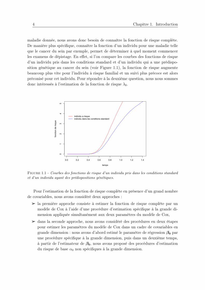
maladie donnée, nous avons donc besoin de connaître la fonction de risque complète.De manière plus spécifique, connaître la fonction d’un individu pour une maladie telleque le cancer du sein par exemple, permet de déterminer à quel moment commencerles examens de dépistage. En effet, si l’on compare les courbes des fonctions de risqued’un individu pris dans les conditions standard et d’un individu qui a une prédispo-sition génétique au cancer du sein (voir Figure 1.1), la fonction de risque augmentebeaucoup plus vite pour l’individu à risque familial et un suivi plus précoce est alorspréconisé pour cet individu. Pour répondre à la deuxième question, nous nous sommesdonc intéressés à l’estimation de la fonction de risque λ0.
0.0 0.2 0.4 0.6 0.8 1.0 1.2 1.4
01
23
45
temps
fon
ctio
n d
e r
isq
ue
individu a risque
individu dans les conditions standard
Figure 1.1 – Courbes des fonctions de risque d’un individu pris dans les conditions standardet d’un individu ayant des prédispositions génétiques.
Pour l’estimation de la fonction de risque complète en présence d’un grand nombrede covariables, nous avons considéré deux approches :
la première approche consiste à estimer la fonction de risque complète par unmodèle de Cox à l’aide d’une procédure d’estimation spécifique à la grande di-mension appliquée simultanément aux deux paramètres du modèle de Cox,
dans la seconde approche, nous avons considéré des procédures en deux étapespour estimer les paramètres du modèle de Cox dans un cadre de covariables engrande dimension : nous avons d’abord estimé le paramètre de régression β0 parune procédure spécifique à la grande dimension, puis dans un deuxième temps,à partir de l’estimateur de β0, nous avons proposé des procédures d’estimationdu risque de base α0 non spécifiques à la grande dimension.
1.1. Cadre de travail 5
1.1.2 Formalisation
Nous utilisons dans la suite le formalisme général des processus de comptage. Pouri = 1, ..., n, nous définissons Ni un processus de comptage marqué 1 et Yi un processusaléatoire à valeurs dans [0, 1]. Nous considérons l’espace probabilisé (Ω,F ,P) et lafiltration (Ft)t≥0 définie par
Ft = σNi(s), Yi(s), 0 ≤ s ≤ t,Zi, i = 1, ..., n,
où Zi = (Zi,1, ..., Zi,p)T ∈ R
p est le vecteur aléatoire de covariables F0-mesurable del’individu i. Notons Λi le compensateur du processus Ni par rapport à (Ft)t≥0, tel queMi = Ni−Λi soit une (Ft)t≥0-martingale. Nous supposons que le processus Ni satisfaitle modèle à intensité multiplicative d’Aalen : pour tout t ≥ 0,
Λi(t) =
∫ t
0
λ0(s,Zi)Yi(s)ds, (1.3)
où λ0 est la fonction de risque (1.2) inconnue à estimer.Nous observons les variables indépendantes et identiquement distribuées (i.i.d.)
(Zi, Ni(t), Yi(t), i = 1, ..., n, 0 ≤ t ≤ τ), où [0, τ ] est l’intervalle de temps entre le débutet la fin de l’étude.
Ce cadre général, introduit par Aalen (1980), inclut plusieurs contextes tels que lesdonnées censurées, les processus de Poisson marqués et les processus de Markov. Nousrenvoyons à Andersen et al. (1993) pour plus de détails.
Cas particulier des données censurées : Dans le cas spécifique de la cen-sure à droite, nous définissons (Ti)i=1,...,n les durées de survie i.i.d. et (Ci)i=1,...,n
les durées de censure i.i.d. de n individus. Nous observons (Xi,Zi, δi)i=1,...,n oùXi = min(Ti, Ci) est la durée jusqu’à la survenue d’un évènement (décès ou censure),Zi = (Zi,1, ..., Zi,p)
T est le vecteur de covariables et δi = 1Ti≤Ci est l’indicateurde censure. La durée de survie Ti est supposée indépendante de la durée de censureconditionnellement au vecteur de covariables Zi pour i = 1, ..., n. Avec ces notations,les processus (Ft)-adaptés Yi et Ni sont respectivement définis par l’indicateur deprésence à risque Yi(t) = 1Xi≥t et le processus de comptage Ni(t) = 1Xi≤t,δi=1 quisaute lorsque le ième individu décède.
Dans la Section 1.1 de l’introduction, nous considérons le cas particulier desdonnées censurées pour simplifier, mais pour toute la suite nous nous plaçons dans lecadre plus général des processus de comptage décrit ci-dessus.
Dans ce cadre de travail, nous avons considéré plusieurs modèles de risque instan-tané λ0.
1. Nous renvoyons à l’Annexe A.1 pour une définition d’un processus de comptage marqué et pourdes rappels généraux sur les processus de comptage

6 Chapitre 1. Introduction
Modèle 1 : Risque non-paramétrique
aucune forme n’est imposée a priori sur λ0 : R+ × R
p → R. (1.4)
Modèle 2 : Modèle de Cox
λ0(t,Z) = α0(t)ef0(Zi), (1.5)
où Zi = (Zi,1, ..., Zi,p)T ∈ R
p est le vecteur de covariables p-dimensionnel del’individu i. Dans ce modèle nous avons considéré :
⊲ le modèle de Cox non-paramétrique : aucune forme a priori n’est imposée niau risque de base α0, ni à la fonction de régression f0 : R
p → R,
⊲ le modèle de Cox semi-paramétrique : aucune forme a priori n’est imposée aurisque de base, mais la fonction de régression est linéaire en les covariablesf0(Z) = βT
0 Z, où β0 ∈ Rp. Ce cas particulier correspond au modèle de Cox
classique (1.1).
Le modèle de Cox non-paramétrique (1.5) a déjà été proposé par Hastie & Tibshi-rani (1986) pour une variable unidimensionnelle et Letué (2000) dans un travailen commun avec Castellan, l’a considéré dans le cas où p < n. Le modèle de Coxsemi-paramétrique (1.1) a été considéré pour la première fois avec le formalismedes processus de comptage par Andersen & Gill (1982). Nous appellerons mo-dèle de Cox non-paramétrique, le modèle (1.5) et simplement modèle de Cox, lemodèle classique (1.1).
1.1.3 Estimation des paramètres du modèle de Cox
Chacun des deux paramètres du modèle de Cox a une interprétation propre. Leparamètre β0 du modèle de Cox traduit le poids des variables explicatives Zi,1, ..., Zi,p
de l’individu i. Lorsque le vecteur de covariables est nul pour l’individu i, la fonctionde risque λ0(.,Zi) de cet individu est alors égale à α0(.). Le risque de base α0(.),comme son nom l’indique, représente donc le risque instantané de décès conditionneld’un individu pris dans des conditions standard, avec les valeurs 0 (de référence) pourles covariables. Nous allons présenter les méthodes classiques d’estimation de ces deuxparamètres lorsque p < n.
1. Estimation du paramètre de régression β0 :
Le paramètre de régression β0 est estimé en minimisant l’opposé de la pseudo-log-vraisemblance de Cox ou log-vraisemblance partielle de Cox introduite parCox (1972) et définie par
l∗n(β) =1
n
n∑
i=1
∫ τ
0
log
(eβ
TZi
Sn(t,β)
)dNi(t), avec Sn(t,β) =
1
n
n∑
i=1
eβTZiYi(t)
(1.6)

1.1. Cadre de travail 7
et Zi = (Zi,1, ..., Zi,p)T ∈ R
p le vecteur de covariables de l’individu i pouri = 1, ..., n. Nous renvoyons à l’Annexe A.2 pour une description de la construc-tion de la log-vraisemblance partielle de Cox à partir de la définition de la log-vraisemblance pour les processus de comptage. La vraisemblance partielle de Coxne fait pas intervenir le risque de base α0. Elle permet donc d’estimer β0 sansavoir à connaître α0. L’estimateur de β0 est alors défini par
β = argminβ∈Rp
−l∗n(β). (1.7)
Le problème (1.7) peut se réécrire sous forme matricielle. Si nous notons U(β) lafonction score, c’est-à-dire le vecteur p× 1 des dérivées premières de l∗n(β), β estsolution de l’équation U(β) = ~0. Il y a en tout, p équations, une pour chacunedes p variables. En général, il n’y a pas de solution explicite. En pratique, onutilise des algorithmes d’optimisation itératifs.
Andersen & Gill (1982) ont prouvé, en utilisant la théorie des processus decomptage, la consistance et la normalité asymptotique de cet estimateur.
2. Estimation du risque de base α0 :
L’estimateur du risque de base est obtenu à partir d’un estimateur du risque debase cumulé. Le risque de base cumulé A0(t) =
∫ τ
0α0(t)dt est estimé, pour un
vecteur β ∈ Rp fixé, par l’estimateur de Nelson-Aalen défini par
A0(t,β) =
∫ t
0
1Y (u)>0Sn(u,β)
dN(u),
où Y = (1/n)∑n
i=1 Yi et N = (1/n)∑n
i=1 Ni. Cet estimateur, introduit par Aalen(1975; 1978), généralise l’estimateur de l’intensité cumulée empirique proposéindépendamment par Nelson (1969; 1972) et Altshuler (1970) dans le cas dedurées de survie censurées.
L’estimateur de Breslow du risque de base cumulé A0(.) est une extension del’estimateur de Nelson-Aalen : on remplace dans l’estimateur de Nelson-Aalen,le paramètre β ∈ R
p fixé, par l’estimateur β défini par (1.7). L’estimateur deBreslow est alors défini par
A0(t, β) =
∫ t
0
1Y (u)>0
Sn(u, β)dN(u). (1.8)
En lissant les incréments de l’estimateur de Breslow (1.8), Ramlau-Hansen(1983b) a proposé un estimateur à noyau du risque de base α0 défini par
αh(t) =1
nh
n∑
i=1
K(t− u
h
)1Y (u)>0
Sn(u, β)dNi(u), (1.9)

8 Chapitre 1. Introduction
où K : R → R est une fonction d’intégrale 1 appelée noyau et h > 0 est lafenêtre. Nous renvoyons à la Section 1.2.3 pour plus de détails sur les estima-teurs à noyau. L’estimateur du risque de base dépend donc de l’estimateur duparamètre de régression β0.
1.1.4 Et quand la dimension augmente...
Les procédures d’estimation et les résultats que nous avons mentionnés en Section1.1.3 ne sont valides que lorsque p < n et même p largement inférieur à n. Lorsquep, le nombre de covariables, grandit, et devient du même ordre de grandeur que n,la taille de l’échantillon, voire plus grand, de nombreux problèmes, maintenant bienconnus, apparaissent. En effet, les résultats de la Section 1.1.3, permettent d’écrire que|β − β0|22 = OP(
pn). Ainsi, dès que p>n, l’estimateur β n’est plus consistant.
Comme nous l’avons déjà dit, le paramètre β0 = (β01 , ..., β0,p) traduit le poidsdes variables explicatives (Z1, ..., Zp) sur la durée de survie T . Lorsque le nombre devariables explicatives est important, un objectif serait d’évaluer la contribution dechaque variable, d’éliminer les variables non pertinentes et donc de sélectionner unsous-ensemble des variables explicatives pertinent, qui permet d’expliquer la durée desurvie T : c’est la sélection de variables. La sélection de variables revient donc à lasélection des coordonnées non nulles dans le vecteur β0. L’idée va donc être de choisir lemeilleur modèle, i.e. le meilleur ensemble de coordonnées non nulles de β0. Le modèlechoisi sera le meilleur au sens d’un critère fixé a priori.
Un critère de qualité classique de choix de modèle, est la valeur de l’opposé de lalog-vraisemblance partielle de Cox (1.6). Plus cette valeur est petite, meilleur est senséêtre le modèle. Autrement dit, on choisira le vecteur qui minimisera cet opposé de lalog-vraisemblance partielle. La vraisemblance (ou la vraisemblance partielle de Cox)est une fonction croissante du nombre de covariables (soit aussi du nombre de coor-données non nulles de β0). Ainsi, minimiser sur un ensemble de modèles, l’opposée dela log-vraisemblance partielle de Cox, en supposant que la minimisation soit possible,conduira immanquablement à choisir le plus grand modèle, autrement dit à choisir unestimateur dont aucune des coordonnées n’est nulle. Outre que cet estimateur peut nepas être défini, même quand il l’est, il restera difficilement interprétable. Pour remé-dier à ces problèmes, une solution classique consiste à pénaliser le critère d’estimation,c’est-à-dire à minimiser l’opposé de la log-vraisemblance partielle de Cox à laquelleon aura ajouté un terme de pénalité, ce qui aura intuitivement tendance à inciter àchoisir un modèle « plus petit »:
β = argminβ∈Rp
−l∗n(β) + pen(β),
où pen : Rp → R+. Dans ce contexte, les pénalités usuelles sont des pénalités qui
sont des fonctions croissantes de la dimension du vecteur covariables. Nous renvoyons

1.1. Cadre de travail 9
à Bickel et al. (2006) pour une réflexion sur le concept de pénalités et sur les diffé-rentes méthodes autour de ce concept. Le choix de la pénalité dépend de la finalité del’étude considérée comme nous allons le voir dans les exemples que nous allons donnerpar la suite. L’objectif de ce type d’approche est de fournir des estimateurs interpré-tables, c’est-à-dire avec peu de coordonnées non nulles correspondant aux variablesqui influencent la durée de survie.
Procédures ℓ0
Un type de pénalité classique, qui permet d’annuler des coordonnées en faisantintervenir la semi-norme ℓ0 du vecteur β, est ce qu’on appelle une pénalité ℓ0 :
pen(β) = Γn|β|0,
où |β|0 est définie par |β|0 =∑p
j=1 1βj 6=0. La définition et la valeur de Γn sontpropres au critère considéré. Deux exemples de critères classiques faisant intervenirla pénalisation ℓ0 sont les critères AIC et BIC. Le critère AIC, introduit par Akaike(1973) est de la forme
penAIC(β) :=2
n|β|0 (1.10)
et le critère BIC, introduit par Schwarz (1978) est défini par
penBIC(β) :=log p
n|β|0, (1.11)
où p est le nombre de covariables.
Le passage à la grande dimension...
Lorsque le nombre de variables explicatives augmente, les procédures de sélectionde variables basées sur les critères AIC et BIC ne sont pas utilisables en pratique.En effet, la complexité algorithmique de ces méthodes est telle, qu’elles sont difficilesà implémenter, même pour des p modestes. Lorsque p augmente et que l’on choisitde faire une comparaison exhaustive de tous les modèles, le nombre de modèles àcomparer augmente en 2p et une étude exhaustive de tous les modèles devient alorsimpossible. Breiman (1995) a ainsi montré que si les problèmes régularisés par unenorme ℓ0 conduisent à des modèles parcimonieux, les estimateurs sont, quant à eux,instables lorsque p grandit.
Les méthodes de sélection de variables considérées précédemment ont été intro-duites dans un cadre classique d’estimation, où la dimension p est raisonnable devantla taille de l’échantillon. Nous avons tendance à parler de grande dimension lorsquep > n. En réalité, déjà lorsque p est de l’ordre de
√n, les algorithmes habituels ne
convergent plus. Nous pouvons donc définir trois régimes : le régime classique, dit depetite dimension, lorsque les algorithmes habituels fonctionnent (généralement pour
10 Chapitre 1. Introduction
p ≤ √n), le régime modéré lorsque p ≥ √
n mais reste de l’ordre de n et le régimede l’ultra grande dimension défini par p ≫ n (d’après Verzelen (2012), le régime del’ultra grande dimension est atteint dès que s log(p/s)/n ≥ 1/2, où s est le nombre decoordonnées non nulles du vecteur β0). Nous parlerons de grande dimension dès quep ≥ √
n, c’est-à-dire dès que les méthodes habituelles ne fonctionnent plus. Dans cemanuscrit, nous considérons des problèmes en grande dimension.
Remarque 1.1 (Le cas de l’ultra grande dimension en pratique). Un domaine oùl’ultra grande dimension, i.e. p ≫ n, est par nature très présente, est le contextede la génomique. En effet, les biotechnologies récentes permettent d’acquérir desdonnées de très grande dimension pour chaque individu. Par exemple, les puces àADN mesurent les niveaux d’expression de dizaines de milliers de gènes simultané-ment. Plus récemment, les NGS pour Séquençage Nouvelle Génération permettentde séquencer l’ensemble du génome d’un individu en l’espace de quelques semaines.Toutefois, ces techniques coûtent encore relativement cher et dans les études classiquesen génomique, le nombre d’individus ne dépasse souvent pas quelques centaines. Sion reprend l’exemple du jeu de données sur le cancer du sein, issu de l’étude de Loiet al. (2007), nous disposons de 44 928 niveaux d’expression de gènes en plus desquatre variables cliniques (âge, taille de la tumeur...) pour 414 patients divisés en deuxgroupes, les patients traités et les patients non traités. Dans cet exemple, le nombre decovariables est très important du fait du nombre de gènes pour lesquels on a mesuré leniveau d’expression, mais aussi du fait du nombre de variables cliniques. Cet exemplecorrespond au cas de ce que nous avons appelé le cas de l’ultra grande dimension(p ≫ n). Cependant, en pratique, il n’est pas raisonnable de considérer l’ensemble descovariables lorsque leur nombre est trop important devant la taille de l’échantillon.Un travail de screening est alors souvent effectué pour faire une première sélectionparmi l’ensemble des covariables et sortir de l’ultra grande dimension. Généralement,on se ramène à p = O(n).
Avant de présenter notre contribution, nous présentons les différentes méthodesd’estimation ainsi que les résultats attendus dans des modèles classiques.

1.2. Généralités sur les méthodes d’estimation et les résultats attendus 11
1.2 Généralités sur les méthodes d’estimation et les
résultats attendus
Dans cette section, nous présentons trois procédures d’estimation : la procédureLasso, la sélection de modèles et l’estimation à noyaux. Ces procédures ont toutes étélargement étudiées en régression additive ou en densité. Dans un souci pédagogique,nous les présentons chacune dans l’un de ces deux cas simples. Les procédures, lesoutils et les résultats obtenus dans ces modèles, sont décrits de façon à illustrer notredémarche, les difficultés rencontrées et la manière dont nous les avons contournées.
1.2.1 La procédure Lasso
La procédure Lasso est l’une des procédures classiques développée en grande di-mension. Elle a été introduite par Tibshirani (1996) dans le cas d’un modèle linéaire.L’estimateur Lasso a ensuite été très largement étudié en régression linéaire (voirKnight & Fu (2000), Efron et al. (2004), Donoho et al. (2006), Meinshausen & Bühl-mann (2006), Zhao & Yu (2006), Zhang & Huang (2008a) et Meinshausen & Yu (2009))et plus généralement dans le cas d’un modèle de régression additive non-paramétrique(voir Juditsky & Nemirovski (2000), Nemirovski (2000), Bunea et al. (2004; 2006;2007a;b), Greenshtein & Ritov (2004) ou encore Bickel et al. (2009)). Enfin, le Lassoou le Dantzig, estimateur proche du Lasso (nous renvoyons à Bickel et al. (2009) pourcomparaison de ces deux estimateurs en régression additive) ont été considérés pourestimer une densité (voir respectivement Bunea et al. (2007c) et Bertin et al. (2011)).
Dans cette sous-section, nous présentons le Lasso dans un cas classique de régressionadditive, en insistant sur la construction de l’estimateur Lasso, les inégalités oraclesnon-asymptotiques recherchées, ainsi que les hypothèses requises.
Modèle illustratif : Dans un modèle de régression additif, soient (Z1,Y1), ..., (Zn,Yn)
un échantillon de n couples indépendants (Zi, Yi) ∈ Rp × R tels que
Yi = f0(Zi) +Wi, i = 1, ..., n, (1.12)
où f0 : Rp → R est une fonction de régression à estimer, les Zi sont déterministes etles erreurs de régression Wi sont centrées et de variance σ2. Les erreurs de régression(Wi)i∈1,...,n, peuvent être de différents types : des erreurs de régression gaussiennessi pour tout i, Wi ∼ N (0, σ2), des erreurs de régression bornées ou plus généralementdes erreurs de régression sous-exponentielles.
Remarque. Si f0(Zi) = βT0 Zi, on obtient le modèle de régression linéaire.
Critère d’estimation : La procédure Lasso est une procédure d’estimation parminimum de contraste pénalisé, fondée sur un critère empirique noté Cn qui dépend des

12 Chapitre 1. Introduction
observations Z1, ..., Zn. En régression additive, le critère d’estimation habituellementconsidéré est le critère des moindres carrés. Il est défini par
Cn(f) =1
n
n∑
i=1
(Yi − f(Zi))2. (1.13)
Dictionnaire de fonction : L’estimation de la fonction de régression f0 non li-néaire repose sur l’idée qu’elle peut être correctement approchée par une combinaisonlinéaire d’un petit nombre de fonctions. On introduit donc un dictionnaire de fonc-tions FM = f1, ..., fM, c’est-à-dire une collection de fonctions fj : Rp → R, pourj = 1, ...,M , à partir desquelles on va construire un estimateur de f0. Le dictionnaireFM est constitué de fonctions de base telles que les ondelettes, les splines, les fonctionsen escaliers, les fonctions coordonnées, etc. Les fonctions fj peuvent aussi être desestimateurs obtenus avec différents paramètres de régularisation.
Fonctions candidates : Les fonctions candidates pour estimer f0 sont des combi-naisons linéaires des fonctions du dictionnaire. Pour β ∈ R
M , on définit la fonctioncandidate fβ telle que
fβ(Zi) =M∑
j=1
βjfj(Zi). (1.14)
Dans le cas particulier où fj(Zi) = Zi,j, le modèle de régression est linéaire avec p = M
et il s’agit d’un problème de sélection de variables. Ainsi, introduire un dictionnairepermet simplement de se placer dans un cadre plus général que celui de la sélectionde variables. Typiquement, la taille du dictionnaire FM utilisé pour estimer une fonc-tion des covariables en grande dimension est grande, i.e. M ≫ n. En considérant desfonctions candidates sous la forme (1.14), on suppose que f0 admet une approxima-tion sparse dans FM , c’est-à-dire qu’on peut l’approcher par une combinaison linéaired’un petit nombre de fonctions de FM . En pratique, le choix du dictionnaire FM estimportant car f0 peut admettre une bonne approximation sparse dans certaines basesde fonctions et pas dans d’autres.
Procédure Lasso : En minimisant le critère (1.13) sur le dictionnaire FM , on seramène alors à un problème d’estimation paramétrique : le paramètre à estimer est leparamètre β de la combinaison linéaire (1.14). L’estimateur Lasso du paramètre β esten fait l’estimateur du minimum de contraste sous une contrainte de type ℓ1 :
βL =
argminβ∈RpCn(fβ),
s.c.p∑
j=1
|βj| ≤ s(1.15)
1.2. Généralités sur les méthodes d’estimation et les résultats attendus 13
où s est un paramètre positif. Nous pouvons réécrire (1.15) sous sa forme pénalisée :
βL = argminβ∈Rp
Cn(fβ) + Γn|β|1, (1.16)
où Γn > 0 est un paramètre de régularisation à calibrer. Les deux notations (1.15) et(1.16) sont équivalentes 2, mais la forme la plus usuelle est celle définie en (1.16) etc’est celle-ci que nous considérerons dans la suite.
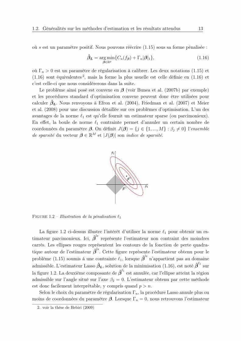
Le problème ainsi posé est convexe en β (voir Bunea et al. (2007b) par exemple)et les procédures standard d’optimisation convexe peuvent donc être utilisées pourcalculer βL. Nous renvoyons à Efron et al. (2004), Friedman et al. (2007) et Meieret al. (2008) pour une discussion détaillée sur ces problèmes d’optimisation. L’un desavantages de la norme ℓ1 est qu’elle fournit un estimateur sparse (ou parcimonieux).En effet, la boule de norme ℓ1 contrainte permet d’annuler un certain nombre decoordonnées du paramètre β. On définit J(β) = j ∈ 1, ...,M : βj 6= 0 l’ensemble
de sparsité du vecteur β ∈ RM et |J(β)| son indice de sparsité.
Figure 1.2 – Illustration de la pénalisation ℓ1
La figure 1.2 ci-dessus illustre l’intérêt d’utiliser la norme ℓ1 pour obtenir un es-
timateur parcimonieux. Ici, βls
représente l’estimateur non contraint des moindrescarrés. Les ellipses rouges représentent les contours de la fonction de perte quadra-
tique autour de l’estimateur βls. Cette figure représente l’estimateur obtenu pour le
problème (1.15) soumis à une contrainte ℓ1, lorsque βls
n’appartient pas au domaine
admissible. L’estimateur Lasso βL, solution de la minimisation (1.16), est noté βℓ1
sur
la figure 1.2. La deuxième composante de βℓ1
est annulée, car l’ellipse atteint la régionadmissible sur l’angle situé sur l’axe β2 = 0. L’estimateur obtenu par cette méthodeest donc facilement interprétable, y compris quand p > n.
Selon le choix du paramètre de régularisation Γn, la procédure Lasso annule plus oumoins de coordonnées du paramètre β. Lorsque Γn = 0, nous retrouvons l’estimateur
2. voir la thèse de Hebiri (2009)

14 Chapitre 1. Introduction
des moindres carrés non-contraint et aucune des coordonnées de β n’est annulée. Enrevanche, pour de très grandes valeurs de Γn, l’estimateur obtenu a toutes ses coor-données nulles, on obtient donc βL = ~0. Il existe plusieurs méthodes permettant dechoisir Γn, mais la plus connue est la validation croisée (voir Tibshirani (1996)).
Remarque. Théoriquement, le paramètre de régularisation Γn est de l’ordre de√logM/n (voir Bühlmann & van de Geer (2009) par exemple). On peut aussi consi-
dérer une procédure Lasso pondéré au sens où la pénalité est en norme ℓ1 pondéréedu paramètre β :
βL = argminβ∈RM
Cn(fβ) + pen(β)
, avec pen(β) =
M∑
j=1
ωj|βj|, (1.17)
et les (ωj)j∈1,...,M sont des poids à déterminer à partir des données (data-drivenweights en anglais). Bickel et al. (2009) ont, par exemple, considéré des poidsωj = Γn||fj||n, où Γn est d’ordre
√logM/n.
Estimateur final : En résolvant (1.17), on obtient l’estimateur Lasso de f0, définipar
fβL(Zi) =
M∑
j=1
βL,jfj(Zi), pour i = 1, ..., n.
Qualité d’estimation : Pour mesurer la qualité d’un estimateur, on cherche à ob-tenir des bornes de risque (risk bound) soit avec grande probabilité pour la normeempirique associée aux moindres carrés définie pour toute fonction f : Rp → R par
||f0 − f ||2n =1
n
n∑
i=1
(f0(Zi)− f(Zi))2,
soit en espérance, c’est-à-dire pour la fonction de perte définie par
ℓ(f0, f) = E[Cn(f)]− E[Cn(f0)] = E
[1
n
n∑
i=1
(f0(Zi)− f(Zi))2
].
Pour l’estimateur Lasso, on trouve par exemple des résultats qui bornent la normeempirique avec grande probabilité (voir Bickel et al. (2009)) ou son espérance commece qu’ont fait par exemple Massart & Meynet (2011).
Nature des résultats :
Trois types de résultats sont classiquement considérés quand p ≥ n. Nous ne men-tionnons ici que les résultats non-asymptotiques.

1.2. Généralités sur les méthodes d’estimation et les résultats attendus 15
— Lorsqu’on cherche à fournir la meilleure approximation du vecteur βT0 Z dans le
cas linéaire ou de f0(Z) dans le cas non-paramétrique, on parle de prédiction. Lesrésultats en prédiction visent à obtenir une majoration pour ||XβL−Xβ0||n, enrégression linéaire, où X est la matrice de design X = (Zi,j)i,j pour i = 1, ..., n
et j = 1, ..., p, et pour ||fβL− f0||n dans le cas non-paramétrique. De très nom-
breux articles se sont intéressés à obtenir des résultats en prédiction dans lemodèle de régression linéaires ou additives. Nous en donnons quelques exemples.Zhang & Huang (2008b) et Bickel et al. (2009) ont obtenu des bornes non-asymptotiques en régression linéaire. Dans le cas non-paramétrique, les perfor-mances en prédiction du Lasso sont mesurées en établissant des inégalités oraclesnon-asymptotiques (voir ci-dessous). Bunea et al. (2007a), Bunea et al. (2007b),Bickel et al. (2009) ou encore Massart & Meynet (2011) ont établi des inégalitésoracles pour l’estimateur Lasso de la fonction de régression.
— Lorsqu’on s’intéresse plutôt à l’estimation du paramètre de régression β0 dans lecas linéaire, on parle d’estimation. Dans un cadre non-asymptotique, les résultatsd’estimation sont souvent exprimés en majorant |β0− βL|1 ou |β0− βL|2 ou plusrarement |β0−βL|q. Bunea et al. (2007a), Bunea (2008) et Bickel et al. (2009) ontainsi obtenu, sous certaines hypothèses, des inégalités en estimation en norme ℓ1,et Bickel et al. (2009), sous des hypothèses plus restrictives, ont aussi établi uneinégalité en sélection en norme ℓq pour 1 < q ≤ 2. Des inégalités en estimationsont obtenues par Meinshausen & Yu (2009) en norme ℓ2 et par Zhang & Huang(2008a) en norme ℓq avec q ≥ 1.
— Si enfin, on veut identifier le support J(β0) = j, β0j 6= 0 de β0, ou encore levecteur signe de β0, on parle de sélection. Les premiers résultats non asymp-totiques de sélection de variables en grande dimension ont été établis dans lecadre de la régression linéaire par Zhao & Yu (2006).
Nous nous intéressons plus particulièrement aux résultats non-asymptotiques en pré-diction et présentons les inégalités oracles ainsi que la démarche pour les établir.
(a) Inégalités oracles pour le Lasso dans le modèle de régression additif
Pour une constante ζ > 0 fixée et un paramètre de régularisation Γn de l’ordrede√
log(M)/n, on définit l’inégalité oracle non-asymptotique pour l’estimateurLasso par
||fβL− f0||2n ≤ (1 + ζ) inf
β∈RM||fβ − f0||2n +Rn,M(β), (1.18)
où ||fβ − f0||2n est un terme de biais et Rn,M(β) est un terme de variance. Cedernier donne la vitesse de convergence de l’estimateur fβL
vers la vraie fonction
16 Chapitre 1. Introduction
f0. Il est d’ordre√
logM/n ou logM/n selon que la convergence de l’estimateurfβL
vers la vraie fonction f0 soit lente ou rapide respectivement. Nous parleronsalors d’inégalité oracle lente ou rapide. Les termes de biais et de variance sontinversement proportionnels à la taille du dictionnaire FM : plus le dictionnairede fonction FM sera grand, plus le terme de biais sera petit et plus le terme devariance sera grand. L’un des objectifs de notre travail est d’établir des inégalitésoracles du type (1.18) avec grande probabilité.
(b) Démarche pour obtenir une inégalité oracle lente
Le début de la démarche pour obtenir des inégalités oracles lentes ou rapidespour l’estimateur Lasso est classique. Par définition du Lasso, on a pour toutβ ∈ R
M ,Cn(fβL
) + pen(βL) ≤ Cn(fβ) + pen(β).
Par définition (1.13) du critère des moindres carrés combiné à un simple jeud’écriture, on obtient finalement
||fβL− f0||2n ≤ ||f0 − fβ||2n +
2
n
n∑
i=1
(fβL− fβ)(Zi)Wi + pen(β)− pen(βL).
Pour tout β ∈ RM , on a fβ =
∑Mj=1 βjfj, en remplaçant fβ et fβL
dans l’inégalitéprécédente on obtient donc finalement
||fβL
− f0||2n ≤ ||fβ − f0||2n + 2
M∑
j=1
(βL − β)jVn(fj) + pen(β)− pen(βL),
avec
Vn(fj) =1
n
n∑
i=1
fj(Zi)Wi. (1.19)
A ce stade, il reste à contrôler le processus Vn(fj) pour obtenir une inégalitéoracle lente. Nous renvoyons au paragraphe (d) pour une discussion sur lecontrôle de ce terme. Pour établir une inégalité oracle rapide, on a besoin d’unehypothèse supplémentaire.
(c) Hypothèse
L’inégalité oracle rapide nécessite une hypothèse supplémentaire sur la matricede Gram Ψn = XTX/n où X = (fj(Zi))i,j avec i ∈ 1, ..., n et j ∈ 1, ...,M.Lorsque M ≫ n, la matrice de Gram Ψn est dégénérée, ce qui s’écrit
minb∈RM\0
(bTΨnb)1/2
|b|2= min
b∈RM\0
|Xb|2√n|b|2
= 0.

1.2. Généralités sur les méthodes d’estimation et les résultats attendus 17
Le problème ordinaire de minimisation des moindres carrés n’a pas de solutionunique, puisqu’il nécessite la définie positivité de la matrice de Gram, c’est-à-dire
minb∈RM\0
|Xb|2√n|b|2
> 0.
La procédure Lasso nécessite une hypothèse plus faible que la définie positivitéde la matrice de Gram.
Nous renvoyons à Bühlmann & van de Geer (2009) et à Bickel et al. (2009) pourdes discussions détaillées sur les différentes hypothèses que l’on peut considérerpour établir une inégalité oracle rapide. Une des hypothèses les plus faibles estla condition aux valeurs propres restreintes (Restricted Eigenvalue condition),introduite par Bickel et al. (2009) pour le modèle de régression additif.
Hypothèse 1.1 (Condition RE(s, c0) pour le modèle de régression additif).Pour un entier s ∈ 1, ...,M et une constante c0 > 0, on dit que la condition
aux valeurs propres restreintes (Restricted Eigenvalue Condition) RE(s, c0) est
vérifiée si
0 < κ(s, c0) = minJ⊂1,...,M,
|J |≤s
minb∈RM\0,
|bJc |1≤c0|bJ |1
(bTΨnb)1/2
|bJ |2, (1.20)
où bJ désigne le vecteur b restreint à l’ensemble J : (bJ)j = bj si j ∈ J et
(bJ)j = 0 si j ∈ J c, où J c = 1, ...,M\J .
La condition aux valeurs propres restreintes assure que la plus petite valeurpropre de la matrice de Gram définie comme
minb∈RM\0
(bTΨnb)1/2
|b|2,
restreinte aux ensembles de sparsités J , tels que |J | ≤ s, soit strictement positive.Autrement dit, la condition RE assure la définie positivité de la matrice Ψn uni-quement pour les vecteurs b ∈ R
M\0 qui vérifient l’inégalité |bJc |1 ≤ c0|bJ |1.L’entier s joue ici le rôle d’une borne supérieure pour l’indice de sparsité |J(β)|associé à un vecteur β, de sorte que les sous-matrices carrées de taille inférieureà 2s de la matrice de Gram Ψn soient définies positives. Dans la démonstrationpermettant d’obtenir l’inégalité oracle rapide, l’hypothèse RE permet de relier lanorme ℓ2 de |(βL−β)J(β)|2 à la norme empirique ||fβL
−fβ||n pour tout β ∈ RM .
(d) Le rôle des inégalités de concentration
Pour que les inégalités oracles soient lentes ou rapides, elles nécessitent le contrôleuniforme du processus Vn(fj) défini par (1.19) (voir paragraphe (b)), souvent à

18 Chapitre 1. Introduction
l’aide d’inégalités de concentration. Bickel et al. (2009) ont utilisé une inégalitéde déviation propre aux variables aléatoires gaussiennes pour contrôler Vn(fj).Lorsque les erreurs de régression Wi pour i = 1, ..., n sont centrées et bornées,on peut appliquer une inégalité de Hoeffding. Dans le cas sous-exponentiel, onutilise une inégalité de Bernstein standard (voir Annexe A.3.1) pour contrôler leprocessus centré Vn(fj). Nous renvoyons à l’Annexe D du Chapitre 2, où nousprésentons une version de la preuve de Bickel et al. (2009) permettant d’obtenirune inégalité oracle lente pour une erreur de régression sous-exponentielle plusgénérale. Le contrôle du processus Vn(fj) par une inégalité de Bernstein y estdétaillé.
1.2.2 La sélection de modèles
La sélection de modèles a d’abord été introduite par Akaike (1973) et Mallows(1973), puis formalisée par Birgé & Massart (1997) pour l’estimation de la densité etpar Barron et al. (1999) dans le cadre plus général d’une fonction inconnue à estimer(densité ou fonction de régression). Elle a été étudiée en régression non-paramétrique(voir entre autres Baraud (2000), Yang (1999), Birgé & Massart (2001), Baraud (2002)ou encore Wegkamp (2003)) et en densité (voir Birgé & Massart (1998) et Birgé (2008)).Nous renvoyons aussi à Massart (2007) comme un ouvrage de référence sur la sélectionde modèles.
Dans cette sous-section, nous expliquons le principe de la sélection de modèles pourl’estimation d’une densité, en détaillant la construction de la procédure de sélection demodèles, les inégalités oracles non-asymptotiques recherchées, ainsi que les hypothèsesrequises.
Modèle : Soient Z1, ..., Zn un n-échantillon de densité f0 inconnue. On suppose quef0 appartient à l’ensemble L
2(R), muni du produit scalaire usuel 〈., .〉 et de la norme||.|| usuelle.
Critère d’estimation et fonction de perte : La procédure de sélection de modèlesest basée, comme la procédure Lasso, sur la minimisation d’un critère d’estimation.Considérons le critère des moindres carrés défini pour la densité par
Cn(f) = ||f ||22 −2
n
n∑
i=1
f(Zi). (1.21)
La pertinence de ce choix est assurée puisque E[Cn(f)] = ||f ||22−2〈f, f0〉2 = ||f− f0||22−||f0||22, qui est minimum en f = f0. La fonction de perte associée est définie pour toutf ∈ L
2(R) par
ℓ(f0, f) = ||f0 − f ||22 =∫
R
(f0(x)− f(x))2dx.
1.2. Généralités sur les méthodes d’estimation et les résultats attendus 19
Bases de fonctions et collection de modèles : Soit (ϕmj )j∈J , où J ⊂ N
∗, unebase de L
2(R). La densité f0 se décompose de manière unique sous la forme
f0 =∑
j∈Jajϕj, avec aj = 〈f0, ϕj〉ϕj.
Pour une collection finie d’indices Mn ⊂ N, on considère la collection de modèles(Sm)m∈Mn
, telle que chaque modèle Sm est engendré par la base (ϕj)j∈Jm , avec Jm ⊂ J :Sm = Vectϕj, j ∈ Jm. La dimension de Sm est alors donnée par Dm := Card(Jm).
Collection d’estimateurs : Associée à cette collection de modèles, on définit lacollection d’estimateurs (fm)m∈Mn
telle que
fm = argminf∈Sm
Cn(f). (1.22)
L’estimateur fm est défini de manière unique par fm =∑
j∈Jm ajϕj, avecaj = (1/n)
∑ni=1 ϕj(Zi). Pour m ∈ Mn, notons
fm = argminf∈Sm
ℓ(f0, f),
la projection orthogonale de f0 sur le modèle Sm. Avec la définition (1.21) de Cn(.),on en déduit que E[fm] = fm. Ainsi, fm est un estimateur sans biais de la projectionde f0 sur le modèle Sm.
Procédure de sélection de modèles : L’objectif est de sélectionner le modèle Sm
parmi l’ensemble des modèles, pour lequel le risque de l’estimateur associé E[ℓ(f0, fm)]
est aussi proche que possible du meilleur des risques que l’on peut obtenir dans lacollection (fm)m∈Mn
. Par le théorème de Pythagore, l’erreur quadratique se décomposeen deux termes :
E[||fm − f0||22] = ||f0 − fm||22 + E[||fm − fm||22]. (1.23)
Le premier terme est le terme de biais, il représente l’erreur d’approximation de f0par fm. Il est d’autant plus petit que Sm est grand. Le second est le terme de va-riance provenant de l’erreur commise en remplaçant aj par une version empirique aj.Contrairement au terme de biais, il est en général d’autant plus grand que le modèleSm est grand. Un choix de modèle optimal en terme d’excès de risque nécessite doncde trouver un compromis entre ces deux termes, i.e., choisir Sm assez grand pour dimi-nuer le biais, mais pas trop pour éviter que la variance n’augmente trop : il s’agit ducompromis biais-variance. L’oracle m∗ est alors l’indice m ∈ Mn qui réalise le meilleurcompromis biais-variance. Il minimise l’excès de risque :
m∗ = argminm∈Mn
E[||fm − f0||22].

20 Chapitre 1. Introduction
L’estimateur oracle associé est alors fm∗ . ll est incalculable en pratique (car m∗ dépendde f0, qui est inconnue) et l’objectif est donc de sélectionner un estimateur fm ayantdes performances similaires à celles de l’oracle. Il s’agit donc de définir un critèrede sélection du modèle imitant le comportement biais-variance (1.25) du risque del’estimateur. Le terme de variance est majoré par
E[||fm − fm||22] ≤1
n
∑
j∈Jm
E[ϕ2j(Zi)] ≤
||f0||∞n
∫
R
∑
j∈Jm
ϕ2j(x)dx = ||f0||∞
Dm
n. (1.24)
On déduit de (1.23) et (1.24), l’inégalité suivante
E[||fm − f0||22] ≤ ||f0 − fm||22 + ||f0||∞Dm
n. (1.25)
On cherche le modèle Sm, sur lequel ||f0 − fm||22 + ||f0||∞Dm/n est minimum. Celarevient à chercher le minimum de −||fm||22 + ||f0||∞Dm/n. Une heuristique que l’ondoit à Mallows (1973) et connue sous le nom d’heuristique de Mallows consiste àremplacer −||fm||22, qui est inconnu, par son estimateur −||fm||22 + ||f0||∞Dm/n, et àprendre m ∈ Mn qui minimise en m le critère
−||fm||22 + 2||f0||∞Dm
n= Cn(fm) + 2||f0||∞
Dm
n. (1.26)
De manière plus générale, le modèle m est sélectionné par la procédure suivante :
m = argminm∈Mn
Cn(fm) + pen(m), (1.27)
où pen : Mn → R+ est de l’ordre du terme de variance E[||fm − fm||22].
Remarque. Dans le cas de la sélection de variables, la taille du modèle correspondau terme |β|0 défini dans la Section 1.1.4. La sélection de modèles avec une pénalitépen(m) = ||f0||∞Dm/n, proportionnelle à la taille du modèle appartient donc bien àla famille des procédures pénalisées en norme ℓ0.
Estimateur final : L’estimateur final, noté fm, est alors obtenu à partir de (1.22)et (1.27). On parle d’estimateur par minimum de contraste pénalisé.
Nature des résultats :
Les inégalités oracles assurent que l’estimateur obtenu par sélection de modèles estperformant. Nous renvoyons à l’ouvrage de Massart (2007) pour plus de détails. Nousprésentons les inégalités oracles en sélection de modèles ainsi que la démarche pour lesétablir.

1.2. Généralités sur les méthodes d’estimation et les résultats attendus 21
(a) Inégalités oracles en sélection de modèles
La qualité de l’estimateur fm est établie via des inégalités oracles de la forme
E[||f0 − fm||22] ≤ C infm∈Mn
||f0 − fm||22 + pen(m)+ C1
n(1.28)
où C est une constante universelle et C1/n un terme négligeable devant l’infi-mum (voir Birgé & Massart (1997)). La constante C1 dépend généralement ducardinal de Mn et de la complexité de la famille de modèles. Le terme de biais||f0 − fm||22 décroît lorsque Dm croît, il dépend de la régularité de f0, inconnue,et est d’autant plus petit que f0 est régulière. Le terme de variance pen(m)
croît avec Dm. Il est d’ordre Dm/n et correspond à l’ordre de la variance sur unmodèle. Ainsi à la constante C près et lorsque le terme résiduel est négligeable,fm réalise le meilleur compromis biais-variance. Le terme résiduel C1/n provientdu contrôle uniforme du processus empirique (1.31), défini ci-dessous, par l’in-égalité de déviation (1.33) (voir les paragraphes (b) et (d) ci-dessous).
(b) Démarche pour obtenir une inégalité oracle
Par définition, l’estimateur fm satisfait pour tout m ∈ Mn l’inégalité suivante :
Cn(fm) + pen(m) ≤ Cn(fm) + pen(m) ≤ Cn(fm) + pen(m). (1.29)
Pour tout f ∈ L2(R), le critère des moindres carrés (1.21) se décompose en
Cn(f) = ||f ||22 − 2〈f0, f〉2 − νn(t) = ||f − f0||22 − ||f0||22 − νn(t), (1.30)
où νn(.) est un processus centré défini par
νn(f) = Cn(f)− E[Cn(f)] = − 2
n
n∑
i=1
f(Zi) + 2
∫
R
f(x)f0(x)dx. (1.31)
En combinant (1.29) et (1.30), on obtient l’inégalité suivante
||f0 − fm||22 ≤ ||f0 − fm||22 + pen(m) + νn(fm)− νn(fm)− pen(m). (1.32)
pour tout m ∈ Mn. Toute la difficulté réside ensuite dans le contrôle uniformedu processus νn(fm)− νn(fm) = νn(fm− fm). Nous renvoyons au paragraphe (d)pour une discussion sur le contrôle de ce processus.
(c) Hypothèses sur les modèles
Les hypothèses suivantes sur les modèles sont standard.

22 Chapitre 1. Introduction
Hypothèse 1.2.
(i) Pour tout m ∈ Mn, Dm ≤ n.
(ii) Il existe une constante φ > 0 telle que pour tout f dans Sm,
||f ||2∞ ≤ φDm||f ||22.
(iii) Les modèles sont emboîtés : Dm1 ≤ Dm2 ⇒ Sm1 ⊂ Sm2.
Nous renvoyons à Birgé & Massart (1998), Barron et al. (1999), Baraud (2002)et Massart (2007) pour des détails sur les hypothèses. L’hypothèse 1.2.(i) per-met d’assurer que la taille des modèles n’est pas trop grande par rapport à lataille de l’échantillon. Si l’on reprend l’exemple de la sélection de variables, lataille d’un modèle correspond au nombre de coefficients inconnus à estimer etl’hypothèse 1.2.(i) impose donc que ce nombre soit inférieur au nombre d’obser-vations. L’hypothèse 1.2.(ii) compare la norme L
2 standard à la norme infinie.Cette hypothèse permet de remplacer, dans la majoration de la variance (1.24),le terme inconnu ||f0||∞ par φ2. Elle est équivalente à l’inégalité suivante (voirle Lemme 1 de Birgé & Massart (1998)) :
∣∣∣∣∣
∣∣∣∣∣∑
j∈Jm
ϕj
∣∣∣∣∣
∣∣∣∣∣
2
∞
≤ φ2Dm.
L’hypothèse 1.2.(iii) est relativement forte. Elle peut dans certains cas êtrerelâchée et remplacée par l’hypothèse de l’existence d’un espace englobant tousles modèles de la collection (voir par exemple l’hypothèse H2 Brunel & Comte(2005)). Cette hypothèse permet de ne pas avoir à parcourir tous les modèles,lors de la procédure de sélection de modèles. En sélection de variables, le nombrede modèles à comparer augmente en 2p lorsque p augmente. Considérer desmodèles emboîtés permet alors de réduire la complexité algorithmique de laprocédure. Les modèles étant emboîtés, on peut considérer le réarrangementsuivant : J = N\0, Jm = 1, ..., Dm et Sm = Vectϕ1, ..., ϕDm
.
Plusieurs bases de fonctions de L2(R) vérifient les hypothèses précédentes et
peuvent être considérées : la base trigonométrique, la base des polynômes parmorceaux, la base d’ondelettes à support compact ou encore la base d’histo-grammes, entre autres. Nous renvoyons à Birgé & Massart (1998), Barron et al.(1999) et Baraud (2002) pour une description détaillée des différentes bases.
(d) Le rôle des inégalités de concentration
D’après l’inégalité (1.32), le processus à contrôler est le processus centréνn(fm − fm), pour m ∈ Mn et νn(.) défini par (1.31). L’idée pour contrôler

1.2. Généralités sur les méthodes d’estimation et les résultats attendus 23
ce processus est de choisir une pénalité qui permette de majorer les variationsde νn(fm − fm). Cependant, ce processus n’est pas facile à contrôler et nécessited’utiliser des techniques spécifiques aux processus empirique. Plus précisément,
νn(fm − fm) ≤ ||fm − fm||2 supf∈Bm,m
νn(f),
où Bm,m′ = f ∈ Sm + Sm′ : ||f ||2 ≤ 1 pour tout m,m′ ∈ Mn. En remplaçantdans l’inégalité (1.32) et en utilisant l’inégalité classique 2xy ≤ b−1x2/ + by2,pour b > 0, on obtient
||f0 − fm||22 ≤ ||f0 − fm||22 + pen(m) + b−1||fm − fm||22 + b supf∈Bm,m
ν2n(f)− pen(m).
L’inégalité de Talagrand définie à l’Annexe A.3.3 est alors l’une des inégalités lesplus utilisées pour contrôler en espérance le supremum d’un processus empirique(voir Massart (2007)). On en déduit une inégalité de déviation de la forme :
Inégalité de déviation 1.1.
∑
m′∈Mn
E
((sup
f∈Bm,m′ν2n(f)− (pen(m) + pen(m′))
)+
)≤ C
n. (1.33)
Cette inégalité de déviation précise comment, dans l’heuristique de Mallows(1.26), l’estimateur du biais ||fm||22 se concentre autour de Dm/n uniformémenten m ∈ Mn.
1.2.3 Estimateurs à noyaux et sélection de fenêtres
Les estimateurs à noyaux sont construits à partir d’une fonction K : R → R,d’intégrale 1, appelée noyau et d’un paramètre réel h > 0, appelé fenêtre. La méthodedes noyaux a été introduite par Rosenblatt (1956) pour estimer une densité f0. Le choixdu noyau se fait parmi un ensemble de noyaux fréquemment utilisés (voir Parzen (1962)et Tsybakov & Zaiats (2009), qui définit six noyaux classiques). Le choix de la fenêtreest crucial et a fait l’objet de nombreuses études. Nous présentons deux méthodes desélection de fenêtres : la validation croisée et la méthode plus récente de Goldenshlugeret Lepski.
Dans cette sous-section, nous expliquons l’idée de la méthode des noyaux dans le casclassique d’estimation d’une densité, nous présentons les deux méthodes de sélectionde fenêtres, puis nous décrivons les inégalités oracles obtenues avec la méthode deGoldenshluger et Lepski et la démarche pour les obtenir.
Modèle : Soient Z1, ..., Zn des variables aléatoires de densité f0 ∈ L2(R) inconnue à
estimer.

24 Chapitre 1. Introduction
Noyau : Le noyau est une fonction K : R → R, intégrable sur R et d’intégrale 1. Ro-senblatt (1956) a considéré un noyau rectangulaire, défini par K(u) = 1]−1;1[(u)/2. Lesnoyaux classiques sont le noyau gaussien K(u) = 1√
2πe−
12u2
et le noyau d’EpanechnikovK(u) = 3
4(1− u2) 1(|u|≤1), parmi les plus utilisés.
Pour tout réel h > 0, on note Kh la fonction définie par Kh : x 7→ K(x/h)/h. Leréel h > 0 est appelé la fenêtre et on introduit la grille de fenêtres Hn.
Collection d’estimateurs : La méthode des noyaux repose sur le principe selonlequel la famille (Kh)h>0 forme une approximation de l’unité pour le produit de convo-lution (voir Komornik (2002) par exemple), i.e. pour tout z ∈ R, la convolée
Kh ∗ f0(z) :=∫
R
Kh(z − u)f0(u)du
converge vers f0(z) en norme L2, quand h tend vers 0. On peut donc approcher f0
par Kh ∗ f0 et comme par définition, Kh ∗ f0(z) = E[Kh(z − Z1)], nous en déduisonsl’estimateur à noyau de la fonction de densité f0 : pour h > 0 fixé et z ∈ R,
fh(z) =1
nh
n∑
i=1
K
(z − Zi
h
). (1.34)
On construit ainsi une famille d’estimateurs (fh)h∈Hn.
Procédure de sélection de fenêtres : Le choix de la fenêtre h (bandwidth enanglais) est très important pour la qualité de l’estimation. La fenêtre optimale h∗ estcelle qui minimise l’excès de risque
h∗ = argminh∈Hn
E[||fh − f0||22],
c’est donc la fenêtre h ∈ Hn qui réalise le meilleur compromis biais-variance dans ladécomposition
E[||fh − f0||22] = ||f0 − fh||22 + E[||fh − fh||22]. (1.35)
Cependant, cette fenêtre n’est pas calculable en pratique puisqu’elle dépend de f0,qui est inconnue. Plusieurs méthodes existent pour sélectionner cette fenêtre. Nous enprésentons ici deux : la méthode de validation croisée et la méthode de Goldenshlugeret Lepski, récemment proposée par Goldenshluger & Lepski (2011).
• Sélection de fenêtres par validation croisée :
Une des méthodes classiquement utilisée en pratique pour choisir la fenêtre h
d’un estimateur à noyau est la méthode de validation croisée (cross-validationen anglais). Cette méthode de sélection de fenêtres a été introduite par Rudemo

1.2. Généralités sur les méthodes d’estimation et les résultats attendus 25
(1982) and Bowman (1984) pour l’estimation de la densité par la méthode desnoyaux.
L’idée de la validation croisée est de proposer un estimateur de l’excès de risqueà partir des données. On a
h∗ = argminh∈Hn
E[||fh − f0||22] = argminh∈Hn
E
∫f 2h(z)dz − 2E
∫fh(z)f0(z)dz.
Considérons l’estimateur
CV(h) =
∫f 2h(z)dz −
2
n
∑
i
fh,−i(Zi), (1.36)
où
fh,−i(Zi) =1
(n− 1)h
∑
j 6=i
K(z − Zj
h
).
L’espérance de la somme dans (1.36) vaut
E
[1
n
∑
i
fh,−i(Zi)
]= E
[∫fh,−n(z)f0(z)dz
]= E
[∫fh(z)f0(z)dz
].
On en déduit que E[CV(h)] = E[||fh − f0||22] −∫f 20 (x)dx et donc que CV(h) +∫
f 20 (x)dx est un estimateur sans biais de l’erreur quadratique moyenne intégrée
E[||fh − f0||22]. La procédure de sélection de fenêtres par validation croisée estalors la suivante
hCV = argminh
CV(h).
L’estimateur à noyau de la densité avec une fenêtre choisie par validation croiséeest alors défini par fhCV .
Les propriétés établies pour l’estimateur à noyau fhCV sont asymptotiques. Pourl’estimation d’une densité, Marron & Padgett (1987) ont montré que la fenêtresélectionnée par validation croisée est optimale au sens où le ratio entre l’erreurquadratique intégrée (ISE pour Integrated Squared Estimator) obtenue par vali-dation croisée et l’infimum de l’ISE obtenu sur toutes les fenêtres converge vers1 presque sûrement. Hall & Marron (1987) ont donné la vitesse de convergencede l’ISE associée à l’estimateur à noyau obtenu par validation croisée. Ils ontaussi prouvé l’optimalité uniforme de ces vitesses pour une classe assez large defonctions de densité.
Mais, à notre connaissance, aucun résultat non-asymptotique n’a été démon-tré pour l’estimateur à noyau avec une fenêtre sélectionnée par validation croisée.
• La méthode de Goldenshluger et Lepski

26 Chapitre 1. Introduction
Récemment, Goldenshluger & Lepski (2011) ont proposé une procédure de sélec-tion de fenêtres pour l’estimation à noyau de la densité d’une variable aléatoiremultivariée et ont établi des inégalités oracles non-asymptotiques pour l’estima-teur ainsi obtenu. Cette procédure a, depuis, été adaptée à différents cadres detravail. Ainsi, elle a par exemple été considérée par Doumic et al. (2012) dansle contexte d’estimation d’un taux de division d’une population structurée entaille dans un cadre non-paramétrique, par Bertin et al. (2013) pour estimer unedensité conditionnelle et par Chagny (2014) pour estimer une fonction réelle àl’aide de noyaux déformés.
Décrivons cette méthode dans le cas plus simple de l’estimation d’une densitéf0. Définissons
fh(z) := E[fh(z)] =1
h
∫
R
K(z − u
h
)f0(u)du = Kh ∗ f0(z), (1.37)
où Kh(z) = (1/h)K(z/h) pour tout z ∈ R et ∗ est le produit de convolutionusuel. Comme pour la procédure de sélection de modèles, le critère de sélectionde fenêtres proposé par Goldenshluger & Lepski (2011) est basé sur une imitationde la décomposition biais-variance (1.35) : il s’agit d’estimer chacun des deuxtermes de la décomposition biais-variance.
D’après la définition (1.37) de fh, le terme de variance est facilement majoré par
E[||fh − fh||22] ≤1
nh
∫
R
K2(u)du ≤ ||K||22nh
. (1.38)
On cherche un estimateur fh dont le risque est aussi proche que possible deminh∈Hn
||f0 − fh||22 + ||K||22/nh. Pour approcher le terme de variance, on posepour tout h ∈ Hn,
V (h) = κ||K||22nh
, (1.39)
où κ > 0 est une constante universelle. La spécificité de la méthode de Gol-denshluger & Lepski (2011) réside dans la façon d’estimer le biais à partir d’unestimateur intermédiaire faisant intervenir deux fenêtres. Plus précisément, leterme de biais est estimé, pour tout h ∈ Hn, par
A(h) = maxh′∈Hn
||fh′ − fh,h′ ||22 − V (h′)
+, (1.40)
où fh,h′(t) = Kh′ ∗ fh(t) est l’estimateur intermédiaire. On peut expliquer cetteestimateur du biais de manière heuristique. L’idée est la suivante : pour être leplus proche possible du terme de biais ||f0 −Kh ∗ f0||22, on remplace la densitéinconnue f0 par l’estimateur fh′ pour une fenêtre h′ ∈ Hn fixée et nous obtenons||fh′ − Kh ∗ fh′ ||22. Mais contrairement au biais, cette quantité contient de la

1.2. Généralités sur les méthodes d’estimation et les résultats attendus 27
variabilité, on lui retire donc un terme V (h′) de l’ordre de la variance. Enfin,comme il n’y a aucune raison de choisir une fenêtre h′ plutôt qu’une autre, onbalaye l’ensemble de la grille Hn.
La procédure de sélection de la fenêtre est définie par
h = argminh∈Hn
A(h) + V (h). (1.41)
Dans la suite, nous ferons référence à cette méthode sous l’appellation « méthodede Goldenshluger et Lepski ».
Estimateur final : L’estimateur à noyau final obtenu avec la méthode de Golden-shluger et Lepski est défini, à partir de (1.34) et (1.41), par fh.
Nature des résultats :
Des inégalités oracles non-asymptotiques ont été établies par Goldenshluger &Lepski (2011) (pour la norme ℓq, q ≥ 1) et par Bertin et al. (2013) pour l’estimateur fhde la densité, dont la fenêtre h a été sélectionnée par la méthode de Goldenshluger etLepski. Nous présentons les inégalités oracles obtenues pour cet estimateur ainsi quela démarche pour les établir.
(a) Inégalités oracles pour l’estimateur à noyau avec une fenêtre sélectionnée par laméthode de Goldenshluger et Lepski
L’objectif dans ce contexte est d’établir des inégalités oracles de la forme
E[||f0 − fh||22] ≤ C infh∈Hn
||f0 − fh||22 + V (h)+Rn (1.42)
où C est une constante universelle et Rn un terme de reste négligeable devantl’infimum. Dans cette inégalité, le terme de biais croît avec h, tandis que leterme de variance V (h) décroît lorsque h augmente.
(b) Démarche pour obtenir une inégalité oracle
On donne ici le début de la démarche pour obtenir une inégalité oracle dans lecas d’un estimateur à noyau fh, obtenu avec la méthode de Goldenshluger etLepski.
D’après la définition (1.40) de A(h), on peut écrire
||fh − f0||22 ≤ 3||fh − fh,h||22 + 3||fh,h − fh||22 + 3||fh − f0||22≤ 3A(h) + 3V (h) + 3A(h) + 3V (h) + 3||fh − f0||22.

28 Chapitre 1. Introduction
De la définition (1.41) de h, on en déduit que
E[||fh − f0||22] ≤ 6E[A(h)] + 6V (h) + 3E[||fh − f0||22]. (1.43)
Le dernier terme de cette inégalité est majoré d’après (1.35) et (1.38) par unterme de biais et un terme de variance du même ordre que V (h). Il reste doncà contrôler E[A(h)] pour obtenir une inégalité oracle de la forme (1.42). Nousrenvoyons au paragraphe (d) pour des détails sur le contrôle de E[A(h)].
(c) Hypothèses sur les noyaux et sur les fenêtres
Pour obtenir une inégalité oracle de la forme (1.42), des hypothèses sur le noyauK et la fenêtre h sont requises.
Hypothèse 1.3.
(i) ||K||∞ = supu∈[−1,1] |K(u)| < ∞.
(ii) nh ≥ 1 et 0 < h < 1.
Les Hypothèses 1.3.(i) et 1.3.(ii) sont standard pour l’estimation à noyau d’unedensité (voir Tsybakov (2004) et Goldenshluger & Lepski (2011)). Elles sontsatisfaites par la plupart des noyaux standard.
(d) Le rôle des inégalités de concentration
Pour obtenir une inégalité oracle de la forme (1.42) à partir de (1.43), il reste àcontrôler E[A(h)]. On décompose A(h) de la façon suivante
3maxh′∈Hn
||fh′−fh′ ||22−
V (h′)
6
+3max
h′∈Hn
||fh,h′−fh,h′ ||22−
V (h′)
6
+3max
h′∈Hn
||fh′−fh,h′ ||22.
Le dernier terme est facilement majoré. Le contrôle en espérance de chacun desdeux premiers termes se fait en utilisant la propriété selon laquelle, pour toutv ∈ L
2(R), ||v||2 = supf∈B〈v, f〉. On définit alors νn,h′(f) = 〈fh′ − fh′ , f〉, et onen déduit que ||fh′ − fh′ ||22 = supf∈B ν2
n,h′(f). En considérant une inégalité deTalagrand définie à l’Annexe A.3.3, nous obtenons, pour l’espérance de chacundes deux premiers termes de la décomposition de A(h), une inégalité de déviationde la forme :
Inégalité de déviation 1.2.
∑
h′∈Hn
E
[supf∈B
ν2n,h′(f)− V (h′)
+
]≤ c
n. (1.44)
Cette inégalité est comparable à l’inégalité de déviation (1.33) en sélection demodèles.

1.2. Généralités sur les méthodes d’estimation et les résultats attendus 29
Comparaison des méthodes de sélection de modèles et de Goldenshlugeret Lepski :
Chagny (2013), dans sa thèse, a mis en évidence les similitudes entre la sélection demodèles et la méthode de Goldenshluger et Lepski. Nous renvoyons à la Table 1.1 dela thèse de Chagny (2013) pour un tableau récapitulatif des éléments clés de chacunedes méthodes dans le cas très simple de l’estimation d’une densité, afin de mettre enévidence ces ressemblances.
1.2.4 Bibliographie en analyse de survie
Nous présentons dans cette sous-section, un état de l’art pour les trois méthodesprésentées ci-dessus (Lasso, sélection de modèles et estimation à noyaux) dans le cadrede l’analyse de survie.
1. La procédure Lasso dans le modèle de Cox usuel
Tibshirani (1997) a proposé une procédure Lasso appliquée à la vraisemblancepartielle de Cox pour estimer le paramètre de régression β0 du modèle de Cox.Cependant, peu de résultats théoriques existent pour cet estimateur Lasso. Nouscommençons par citer un premier résultat asymptotique : Bradic et al. (2012) ontétabli une inégalité asymptotique en estimation en norme ℓ2 pour l’estimateurLasso du paramètre de régression du modèle de Cox semi-paramétrique (1.1).Les résultats non-asymptotiques pour l’estimateur Lasso dans le modèle de Coxn’ont été établis que très récemment. Kong & Nan (2012) and Bradic & Song(2012) ont obtenus des résultats de prédiction sous forme d’inégalités oraclespour la fonction de régression du modèle de Cox non-paramétrique (1.5). Huanget al. (2013) ont, quant à eux, obtenu un résultat en prédiction et des résultatsen estimations en normes ℓ1, ℓ2 et en norme ℓq avec q ≥ 1 pour le modèle de Coxsemi-paramétrique (1.1).
Des extensions du Lasso ont aussi été proposées pour estimer la partie paramé-trique du modèle de Cox (1.1). L’adaptive Lasso a été considéré par Zhang & Lu(2007), qui ont obtenu un résultat asymptotique d’estimation et par Zou (2008),qui a assuré un résultat de consistance en sélection. Antoniadis et al. (2010) ontétabli une inégalité asymptotique en estimation pour l’estimateur de Dantzigdans le modèle de Cox semi-paramétrique (1.1) (nous renvoyons à Bickel et al.(2009) pour une comparaison entre l’estimateur Lasso et l’estimateur de Dantzigdans le modèle de régression additif (1.12)).
Plus généralement, en analyse de survie, le Lasso a aussi été utilisé dans le casd’un modèle additif d’Aalen (cf. Andersen et al. (1993) pour une description dece modèle) par Martinussen & Scheike (2009) et Gaïffas & Guilloux (2012). Cesderniers ont obtenu une inégalité oracle non-asymptotique pour la fonction des

30 Chapitre 1. Introduction
covariables du modèle.
2. La sélection de modèles
La méthode d’estimation non-paramétrique par sélection de modèles a été adap-tée à l’analyse de survie dans différents modèles. Letué (2000) a adapté cetteméthode pour estimer en petite dimension (p < n), la fonction de régression f0du modèle de Cox non-paramétrique (1.5). Pour cela, elle a considéré le contrastede la log-vraisemblance partielle de Cox associé à une fonction de perte du typeinformation de Kullback-Leibler et elle a obtenu pour son estimateur une inéga-lité oracle de la forme (1.42). Plus récemment, Brunel & Comte (2005), Brunelet al. (2009) et Brunel et al. (2010) ont considéré la méthode de sélection demodèles pour estimer une densité dans le cas de données censurées.
Dans un contexte plus proche du nôtre, la méthode de sélection de modèles aété utilisée pour estimer l’intensité d’un processus de comptage dans un modèleà intensité multiplicative d’Aalen (1.3). Reynaud-Bouret (2006) a établi desinégalités oracles pour l’estimateur par minimum de contraste pénalisé de lafonction de risque sans covariable. Comte et al. (2011) ont aussi considéré lasélection de modèles pour estimer une fonction de risque non-paramétrique (enpetite dimension). Ils ont appliqué la sélection de modèles en deux directions,selon le temps et selon les covariables, et ont obtenu une inégalité oracle pourleur estimateur.
3. L’estimation à noyaux
L’estimateur à noyau pour la fonction de risque a d’abord été proposé par Wat-son & Leadbetter (1964a;b) dans le cas de données non-censurées, ses propriétésont ensuite été étudiées par Rice & Rosenblatt (1976). Ramlau-Hansen (1983b) aintroduit l’estimateur à noyau pour estimer l’intensité d’un processus de comp-tage et a étendu son utilisation à des données de survie censurées. Il a ainsiproposé l’estimateur à noyau (1.9) du risque de base dans le modèle de Cox.
Comme pour l’estimation d’une densité, le choix de la fenêtre est crucial. Maistrès peu de résultats existent en survie. Essentiellement deux méthodes decalibration adaptatif de fenêtre ont été considérées en analyse de survie. La plusancienne est basée sur la validation croisée. La seconde est basée sur la méthodede Goldenshluger et Lepski. La méthode de validation croisée dans un modèle àintensité multiplicative d’Aalen pour les processus de comptage a été suggéréepar Ramlau-Hansen (1981). Grégoire (1993) a prouvé la consistance en 1/n
de l’estimateur de l’erreur quadratique intégrée associé à l’estimateur à noyauobtenu par validation croisée de l’intensité d’un processus de comptage dansle modèle à intensité multiplicative d’Aalen. Cependant, à notre connaissance,aucun résultat non-asymptotique n’a été établi pour l’estimateur à noyau obtenu

1.2. Généralités sur les méthodes d’estimation et les résultats attendus 31
par validation croisée de l’intensité. La méthode de Goldenshluger et Lepski aété considérée par Bouaziz et al. (2013) pour estimer l’intensité de processus decomptage des évènements récurrents (cadre différent de celui qui nous intéresseici). Ils ont obtenu une inégalité oracle non-asymptotique pour l’estimateurobtenu.
Nous décrivons dans la suite de l’introduction, nos propres contributions.

32 Chapitre 1. Introduction
1.3 Cheminement et principaux résultats
Rappelons le cadre de travail. Nous observons n copies indépendantes(Zi, Ni(t), Yi(t), i = 1, ..., n, 0 ≤ t ≤ τ), où Zi = (Zi,1, ..., Zi,p)
T ∈ Rp est le vec-
teur de covariables, Ni un processus de comptage marqué, Yi un processus aléatoire àvaleurs dans [0, 1] et [0, τ ] un intervalle de temps. À partir de ces observations, nouscherchons à estimer la fonction de risque λ0(.,Zi).
I. La Partie I est consacrée à l’estimation en grande dimension de la fonction derisque non-paramétrique λ0, satisfaisant un modèle à intensité multiplicatived’Aalen défini, pour tout t ≥ 0, par
Λ(t) =
∫ t
0
λ0(s,Z)Y (s)ds,
où Z ∈ Rp est le vecteur générique de covariables de même loi que les vecteurs de
covariables Zi pour chaque individu i. Nous estimons cette fonction de risque parun modèle de Cox non-paramétrique constitué de deux paramètres fonctionnelsinconnus. Nous proposons de l’estimer à l’aide d’une procédure Lasso simultanée.
II. La Partie II est consacrée à l’estimation du risque de base dans un modèle deCox semi-paramétrique usuel, où la fonction de risque s’écrit
λ0(t,Z) = α0(t)eβT0Z .
Dans ce modèle, le paramètre β0 a une dimension p supérieure à la taille del’échantillon n. Comme nous l’avons vu dans la Section 1.1.3, l’estimation durisque de base requiert l’estimation préalable du paramètre de régression. Nousavons ainsi proposé des procédures d’estimation du risque de base constituée dedeux étapes :
— la première étape, commune aux deux procédures considérées, porte surl’estimation du paramètre de régression β0 à l’aide d’une procédure Lasso,telle que celle décrite par Huang et al. (2013),
— la deuxième étape porte sur la construction d’un estimateur du risque debase α0. Nous avons proposé deux méthodes d’estimation de α0. Ces estima-teurs appartiennent chacun à l’une des deux grandes familles d’estimateursnon-paramétriques : estimateur par sélection de modèles et estimateur ànoyaux. Le choix de la fenêtre de l’estimateur à noyau découle d’une adap-tation de la méthode de Goldenshluger et Lepski.
Nous avons implémenté les procédures d’estimation de la Partie II, afin de com-parer les deux méthodes d’estimation du risque de base.
Dans les deux parties, nous avons établi des inégalités oracles non-asymptotiques.

1.3. Cheminement et principaux résultats 33
D’après les Sections 1.2.1 et 1.2.2, les procédures Lasso et de sélection de mo-dèles requièrent le choix d’un critère d’estimation. Nous définissons les critères de lavraisemblance et des moindres carrés usuels pour les processus de comptage.
La vraisemblance empirique totale (utilisée au Chapitre 2)D’après la formule de Girsanov ou de Jacod (1973; 1975) (voir également Andersenet al. (1993)), le critère de la log-vraisemblance pour une fonction λ : [0, τ ]×R
p → R,est donné par
Cn(λ) = − 1
n
n∑
i=1
∫ τ
0
log λ(t,Zi)dNi(t)−∫ τ
0
λ(t,Zi)Yi(t)dt
. (1.45)
Ce critère d’estimation est utilisé dans le Chapitre 2. Il présente l’avantage depermettre l’estimation de la fonction de risque complète. La fonction de perte clas-siquement associée à ce critère est la divergence de Kullback (nous renvoyons à laSection 1.3.1 pour des détails concernant cette fonction de perte). Notons que la vrai-semblance partielle de Cox, définie par (1.6), est obtenue à partir de la vraisemblance(1.45). Nous renvoyons à l’Annexe A.2 pour les détails concernant les liens entre lesdeux.
Le contraste des moindres carrés (utilisé au Chapitre 3)Le critère des moindres carrés pour les processus de comptage a été considéré parReynaud-Bouret (2006) et Comte et al. (2011). Il est défini pour une fonction λ :
[0, τ ]× Rp → R par
Cn(λ) =1
n
n∑
i=1
∫ τ
0
λ2(t,Zi)Yi(t)dt−2
n
n∑
i=1
∫ τ
0
λ(t,Zi)dNi(t). (1.46)
Nous aurions pu utiliser ce critère pour estimer la fonction de risque complète, cepen-dant le processus empirique qui en découle n’est pas linéaire en λ et est donc difficileà contrôler. Nous l’avons plutôt considéré, dans une version modifiée, pour estimer lerisque de base du modèle de Cox au Chapitre 3 (voir Section 1.3.2 pour les détails). Lecritère des moindres carrés est relié à la norme empirique plus facilement interprétable.
1.3.1 Partie I : Estimation de l’intensité complète d’un proces-sus de comptage par un modèle de Cox
1. Le modèle
Considérons le cadre général des processus de comptage décrit à la Section 1.1avec pour i = 1, ..., n, le processus de comptage marqué Ni satisfaisant le modèle

34 Chapitre 1. Introduction
à intensité multiplicative d’Aalen (1.3). Nous ne faisons aucune hypothèse sur laforme de la fonction de risque λ0, en particulier, nous ne supposons pas que λ0
vérifie un modèle de Cox.
D’après la décomposition de Doob-Meyer, on peut heuristiquement écrire quepour tout i ∈ 1, ..., n,
dNi(t) = λ0(t,Zi)Yi(t)dt+ dMi(t).
Si l’on compare au Modèle de régression additif (1.12), dMi(.) peut être interprétécomme un terme de bruit de type sous-exponentiel.
Notre objectif est d’estimer de manière non-paramétrique la fonction de risqueλ0 par un modèle de Cox non-paramétrique, c’est-à-dire par une fonction dela forme λ(t,Z) = α(t)ef(Z), où la fonction du temps α et la fonction descovariables f sont à estimer.
2. La procédure d’estimation
En suivant les étapes du paragraphe 1.2.1 pour le modèle de régression additif,nous décrivons la mise en oeuvre de la procédure Lasso dans le modèle à intensitémultiplicative d’Aalen.
Choix du critère d’estimation : Nous avons choisi le critère de la vraisem-blance empirique totale (1.45). C’est le critère qui s’est avéré le plus pertinentpour estimer la fonction de risque et obtenir des inégalités oracles pour l’esti-mateur obtenu. En effet, contrairement au critère des moindres carrés, à partirduquel nous obtenons un processus empirique non linéaire en les fonctions quel’on cherche à estimer, les processus empiriques qui découlent du critère de lavraisemblance total sont linéaires en les fonctions à estimer (nous renvoyons auparagraphe 5. pour la définition de ces processus).
Dictionnaires de fonctions : Notre modèle fait intervenir, non pas un para-mètre à estimer, comme c’est le cas dans le modèle de régression additif ou dansle modèle de Cox non-paramétrique lorsque l’on ne s’intéresse qu’à la fonction derégression, mais deux paramètres à estimer. Nous estimons ces deux paramètresfonctionnels par des combinaisons linéaires de fonctions. Nous introduisons doncdeux dictionnaires de fonctions : un dictionnaire de fonctions des covariablesFM = f1, ..., fM, où fj : R
p → R pour j = 1, ...,M et un dictionnaire des fonc-tions du temps GN = θ1, ..., θN, où θk : R
+ → R pour k = 1, ..., N . La taille dudictionnaire FM utilisé pour estimer la fonction des covariables en grande dimen-sion est grande , i.e. M ≫ n, alors que pour estimer une fonction sur R
+, nousconsidérons un dictionnaire GN de taille de l’ordre de la taille de l’échantillon n.

1.3. Cheminement et principaux résultats 35
Fonctions candidates : Ensuite, comme dans le modèle de régression additif,nous déterminons des fonctions candidates pour estimer l’intensité complète λ0,mais dans notre cas, non plus à partir d’un seul dictionnaire, mais à partir desdeux dictionnaires FM et GN . Comme nous cherchons à estimer la fonction derisque par un modèle de Cox, nous considérons des fonctions candidates de laforme
λβ,γ(t,Zi) = αγ(t)efβ(Zi),
avec (β,γ) ∈ RM × R
N et
logαγ =N∑
k=1
γkθk et fβ =M∑
j=1
βjfj.
Procédure Lasso simultanée : Nous estimons les deux paramètres vectorielsβ et γ simultanément à l’aide d’une procédure Lasso pondéré. Nous avons pourcela considéré la procédure suivante :
(βL, γL) = argmin(β,γ)∈RM×RN
Cn(λβ,γ) + pen(β) + pen(γ), (1.47)
avec
pen(β) =M∑
j=1
ωj|βj| and pen(γ) =N∑
k=1
δk|γk|,
(ωj)j∈1,...,M et (δk)k∈1,...,N sont des poids à déterminer.
Estimateur final : En appliquant la procédure (1.47) au critère de la vrai-semblance (1.45), nous obtenons finalement l’estimateur Lasso suivant :
λβL,γL(t,Zi) = αγL(t)e
fβL
(Zi).
3. Les fonctions de perte
La fonction de perte associée au critère d’estimation (1.45) est la divergence deKullback empirique définie par
Kn(λ0, λβ,γ) =1
n
n∑
i=1
∫ τ
0
(log λ0(t,Zi)− log λβ,γ(t,Zi))λ0(t,Zi)Yi(t)dt (1.48)
− 1
n
n∑
i=1
∫ τ
0
(λ0(t,Zi)− λβ,γ(t,Zi))Yi(t)dt. (1.49)
Dans cette définition, le premier terme (1.48) correspondrait à la divergence deKullback usuelle si λ0(t,Zi) et λ(t,Zi) étaient des densités. Cependant, commela fonction de risque n’est pas une densité, le terme résiduel (1.49) intervient.
36 Chapitre 1. Introduction
Nous renvoyons à van de Geer (1995) et Senoussi (1988) pour des définitionssimilaires de divergences de Kullback empiriques.
Les qualités des estimateurs sont également évaluées par la fonction de pertedéfinie pour toute fonction h sur [0, τ ]× R
p par
||h||n,Λ =
√√√√ 1
n
n∑
i=1
∫ τ
0
(h(t,Zi))2dΛi(t). (1.50)
Dans cette définition, plus l’intensité du processus Ni est grande, plus la contri-bution de l’individu i dans cette norme empirique est importante. Nous avonsmontré que cette norme est reliée à la divergence de Kullback empirique.
Pour plus de clarté, nous avons résumé dans un tableau comparatif (voir Table1.1) les éléments clés de la démarche associée à la procédure Lasso pour le Mo-dèle de régression additif (1.12) et pour notre Modèle à intensité multiplicatived’Aalen (1.3) non-paramétrique.
4. Les hypothèses
Comme dans le cas de la régression additive, une hypothèse sur la matricede Gram est nécessaire afin d’établir une inégalité oracle rapide. Dans notrecontexte, la matrice de design est définie par
X(t) =
θ1(t) . . . θN(t)
X...
...θ1(t) . . . θN(t)
∈ R
n×(M+N),
où X = (fj(Zi))i,j pour i = 1, ..., n et j = 1, ...,M . Elle fait intervenir lesfonctions des deux dictionnaires. La matrice de Gram associée est donnée par
Gn =1
n
∫ τ
0
X(t)T C(t)X(t)dt,
avec C(t) = (diag(λ0(t,Zi)Yi(t)))1≤i≤n, ∀t ≥ 0. Habituellement, on applique lacondition aux valeurs propres restreintes (1.20) à la matrice de Gram. Cependant,la matrice Gn est aléatoire, même conditionnellement aux covariables. Nousimposons donc plutôt une condition aux valeurs propres restreintes à E(Gn), oùl’espérance est prise conditionnellement aux covariables.
Hypothèse 1.4. Pour un entier s ∈ 1, ...,M + N et une constante r0 > 0,
E[Gn] satisfait la condition aux valeurs propres restreintes RE(s, r0) si :
0 < κ0(s, r0) = minJ⊂1,...,M+N,
|J |≤s
minb∈RM+N\0,|bJc |1≤r0|bJ |1
(bTE(Gn)b)1/2
|bJ |2.

1.3.C
heminem
entet
principauxrésultats
37Modèle de régression additif Modèle de Cox non-paramétrique
Modèle Y = f0(Z) +W λ0(t,Z) = α0(t)ef0(Z)
Paramètres f0 fonction des covariables f0 fonction des covariablesinconnus α0 fonction du temps
Dictionnaires FM = f1, ..., fj, fj : Rp → R FM = f1, ..., fj, fj : R
p → R
GN = θ1, ..., θN, θk : R+ → R
Candidats fβ(Z) =M∑
j=1
βjfj(Z) λβ,γ(t,Z) = αγ(t)efβ(Z), logαγ =
N∑
k=1
γkθk et fβ =
M∑
j=1
βjfj
Critères Moindres carrés Log-vraisemblance empirique totale
d’estimation Cn(fβ) =1n
n∑
i=1
(Yi − fβ(Zi))2 Cn(λβ,γ) = − 1
n
n∑
i=1
∫ τ
0log λβ,γ(t,Zi)dNi(t)−
∫ τ
0λβ,γ(t,Zi)Yi(t)dt
Estimateurs βL = argminβ∈RM
1n
n∑
i=1
(Yi − fβ(Zi))2 + pen(β)
(βL, γL) = argmin
(β,γ)∈RM×RN
Cn(λβ,γ) + pen(β) + pen(γ)
Perte empirique ||fβ − f0||2n = 1n
n∑
i=1
(fβ − f0)2(Zi) ||λβL,γL
− λ0||2n,Λ = 1n
n∑
i=1
∫ τ
0
(λβL,γL− λ0)
2(t,Zi)2dΛi(t)
Table 1.1 – Tableau comparatif pour la procédure Lasso dans le modèle de régression additif et dans le modèle à intensité multiplicatived’Aalen non-paramétrique.

38 Chapitre 1. Introduction
Nous avons montré, que si la condition RE est vérifiée pour E(Gn), alors laversion empirique de la condition RE appliquée à Gn est satisfaite avec grandeprobabilité. Cette hypothèse nous permet de relier la norme ℓ2 à la norme em-pirique pondérée ||.||n,Λ.
Cette version modifiée de la condition aux valeurs propres restreintes est nou-velle, et c’est la première fois à notre connaissance qu’une inégalité oraclenon-asymptotique rapide est établie sous une telle hypothèse.
5. Les processus empiriques et les inégalités de concentration
En suivant la même démarche de preuve que celle détaillée pour le modèle derégression additif, on a pour tout (β,γ) in R
M × RN ,
Cn(λβL,γL) + pen(βL) + pen(γL) ≤ Cn(λβ,γ) + pen(β) + pen(γ),
et les processus à contrôler sont définis par
ηn,t(fj) =1
n
n∑
i=1
∫ t
0
fj(Zi)dMi(s) et νn,t(θk) =1
n
n∑
i=1
∫ t
0
θk(s)dMi(s).
Pour contrôler ces processus, nous avons établi de nouvelles inégalités de Bern-stein empiriques pour les martingales à sauts.
Ces inégalités de Bernstein sont cruciales pour déterminer les poids ωj et δk, desorte que |ηn,τ (fj)| ≤ ωj (respectivement |νn,τ (θk)| ≤ δk) avec grande probabilité.Nous obtenons des poids de l’ordre de
ωj ≈√
logM
nVn,τ (fj) et δk ≈
√logN
nRn,τ (θk).
L’introduction de poids dans la procédure Lasso en analyse de survie avait déjàété considérée par Gaïffas & Guilloux (2012) pour le modèle additif d’Aalen,mais jamais pour un modèle multiplicatif.
6. Le résultat principal
Nous avons établi les premières inégalités oracles non-asymptotiques rapides endivergence de Kullback empirique et en norme empirique pondérée pour l’esti-mateur Lasso simultanée de la fonction de risque complète en grande dimensionsous une nouvelle condition aux valeurs propres restreintes. Nous en donnons iciune version simplifiée.

1.3. Cheminement et principaux résultats 39
Résultat 1.1 (Théorème 2.4 dans Lemler (2012)). Supposons l’hypothèse RE
satisfaite pour certaines constantes par la matrice E[Gn]. Alors, avec grande
probabilité,
Kn(λ0, λβL,γL) ≤ (1 + ζ) inf
(β,γ)
Kn(λ0, λβ,γ) + C(β,γ) max
1≤j≤M
1≤k≤N
ω2j , δ
2k,
et
|| logλ0 − log λβL,γL||2n,Λ
≤ (1 + ζ) inf(β,γ)
|| log λ0 − log λβ,γ ||2n,Λ + C ′(β,γ) max
1≤j≤M
1≤k≤N
ω2j , δ
2k,
où C > 0 et C ′ > 0 sont des constantes.
Nous obtenons une inégalité oracle non-asymptotique rapide en prédiction. Eneffet, la vitesse de convergence de cette inégalité est d’ordre
(max
1≤j≤M
1≤k≤N
ωj, δk)2
≈ max logM
n,logN
n
. (1.51)
Cette vitesse de convergence fait apparaître les deux vitesses de convergenceque nous aurions attendu si nous avions considéré l’estimation des deux partiesdu modèle de Cox séparément. Ici, l’estimation de la fonction de risque par unmodèle de Cox non-paramétrique implique deux parties différentes : la premièrepartie est le risque de base αγ : R → R et la seconde partie est la fonction descovariables fβ : Rp → R. La double pénalisation ℓ1 considérée vise à estimersimultanément la fonction f0 des covariables en grande dimension et la fonctionnon-paramétrique α0. Comme les deux paramètres f0 et α0 sont estimés simulta-nément, nous obtenons une vitesse de convergence qui fait apparaître les vitessesde convergence de chacune des deux parties de l’estimation. Cependant, si nousconsidérons le point de vue de Bertin et al. (2011), nous pouvons nous attendreà ce qu’un choix de N d’ordre n permette d’estimer correctement la fonctiondu temps. Par conséquent, dans un contexte de très grande dimension, le termedominant dans (1.51) sera d’ordre logM/n, ce qui est la vitesse caractéristiqued’une inégalité oracle rapide.
Les travaux de la Partie I font l’objet d’un article soumis pour publication, et ac-cepté aux Annales de l’Institut Henri Poincaré :S. Lemler. (2012), Oracle inequalities for the lasso in the high-dimensional multipli-
cative Aalen intensity model. arXiv preprint arXiv:1206.5628. http://arxiv.org/pdf/1206.5628v4.pdf.

40 Chapitre 1. Introduction
1.3.2 Partie II : Estimation adaptative de la fonction de basedans le modèle de Cox
1. Le modèle
Nous considérons le modèle de Cox : pour tout t ∈ [0, τ ]
λ0(t,Zi) = α0(t)eβT0Zi ,
où Zi = (Zi,1, ..., Zi,p)T ∈ R
p et i = 1, ..., n, et où le vecteur de covariablesest de grande dimension (cf. Section 1.1.4). Le risque de base est une fonctiondu temps de R
+ dans R. Nous avons établi un premier résultat en considérantune procédure Lasso pour estimer les deux paramètres du modèle de Cox, ilest aussi intéressant de considérer une procédure en deux étapes en estimantle paramètre de régression β0 par une procédure Lasso et en considérant desprocédures d’estimation du risque de base qui ne soient pas spécifiques à lagrande dimension.
2. Les procédures d’estimation
Première étape : estimation du paramètre de régression β0
Pour estimer le paramètre de régression β0 du modèle de Cox en grande dimen-sion, nous considérons une procédure Lasso appliquée à la vraisemblance partiellede Cox (1.6) :
β = argminβ∈Rp
−l∗n(β) + Γn|β|1, (1.52)
où Γn est d’ordre√log(pn)/n. À partir d’un résultat de Huang et al. (2013),
nous avons montré la proposition suivante.
Proposition 1.1. Soit k > 0 et c > 0. Supposons que les covariables Zi,j sont
bornées pour tout i ∈ 1, ..., n et j ∈ 1, ..., p. Alors, avec probabilité supérieure
à 1− cn−k, nous avons
|β − β0|1 ≤ C(s)
√log(pnk)
n,
où C(s) > 0 est une constante qui dépend de l’indice de sparsité s = |J0| de β0.
Cette proposition donne une borne non-asymptotique en prédiction crucialepour établir les inégalités oracles pour les deux estimateurs du risque de base.
Deuxième étape : les procédures d’estimation du risque de base α0

1.3. Cheminement et principaux résultats 41
(a) Sélection de modèles :
Nous avons considéré la procédure classique de sélection de modèles.
Critère d’estimation et fonction de perte : Nous avons choisi detravailler avec un critère type moindres carrés :
Cn(α,β) = − 2
n
n∑
i=1
∫ τ
0
α(t)dNi(t) +1
n
n∑
i=1
∫ τ
0
α2(t)eβTZiYi(t)dt. (1.53)
Ce critère ne correspond pas tout à fait au critère des moindres carrés(1.46) appliqué à la fonction de risque λ(t,Zi) = α(t)eβ
TZi puisque nousavons enlevé dans chaque terme du contraste Cn, une exponentielle. Nousavons montré qu’il est pertinent de considérer ce critère pour estimer α0. Lecritère (1.53) fait apparaître les deux paramètres du modèle de Cox α et β.Nous considérons ce critère en β = β défini par (1.52), ceci explique le faitque l’estimateur du risque de base dépend de l’estimateur du paramètre derégression. Associée à ce critère, nous avons considéré la norme déterministesuivante :
||α||2det =∫ τ
0
α2(t)E[eβT0Z1Y1(t)]dt. (1.54)
Comme nous l’avons vu, les inégalités oracles reposent sur des comparaisonsde norme. Ici, une partie du travail consiste donc à comparer la normedéterministe (1.54) à la norme L
2 standard.
Bases de fonctions et collection de modèles : Soit Mn un ensembled’indices et Sm,m ∈ Mn une collection de modèles définis par
Sm = α : α(t) =∑
j∈Jm
amj ϕmj (t), a
mj ∈ R,
où (ϕmj )j∈Jm est une base orthonormale de (L2 ∩ L
∞)([0, τ ]). On note Dm
le cardinal de Sm, i.e. |Jm| = Dm.
Collection d’estimateurs : La collection d’estimateurs (αβm)m∈Mn
surune collection de modèles Sm : m ∈ Mn, est telle que :
αβm = argmin
α∈Sm
Cn(α, β).
Procédure de sélection de modèles : La procédure de sélection demodèles est donnée par :
mβ = argminm∈Mn
Cn(αβm, β) + pen(m).

42 Chapitre 1. Introduction
Estimateur final : L’estimateur par minimum de contraste pénalisé estalors défini par αβ
mβ.
(b) Estimateur à noyau et méthode de Goldenshluger et Lepski :
Collection d’estimateurs : Considérons l’estimateur à noyau usuel, in-troduit par Ramlau-Hansen (1983b), pour estimer le risque de base :
αβh (t) =
1
nh
n∑
i=1
∫ τ
0
K(t− u
h
)1Y (u)>0
Sn(u, β)dNi(u), (1.55)
avec
Y =1
n
n∑
i=1
Yi, et Sn(u, β) =1
n
n∑
i=1
eβTZiYi(u),
dans lequel nous injectons l’estimateur Lasso β défini par (1.52). Nous ob-
tenons ainsi une collection d’estimateurs (αβh )h∈Hn
, où Hn est une grille defenêtres, choisie judicieusement.
Procédure de sélection de fenêtres : Nous proposons une procédurede sélection de fenêtres par la méthode de Goldenshluger et Lepski :
hβ = argminh∈Hn
Aβ(h) + V (h),
avecAβ(h) = sup
h′∈Hn
||αβ
h,h′ − αβh′ ||22,ε − V (h′)
+
et αβh,h′(t) = Kh′ ∗ αβ
h (t). La norme ||.||2,ε correspond à la norme surL2([ε, τ − ε]), où ε = maxh : h ∈ Hn.
Estimateur final : L’estimateur à noyau avec une fenêtre sélectionnéepar la méthode de Goldenshluger et Lepski est alors défini par αβ
hβ.
Nous avons contruit un tableau récapitulatif et comparatif des procéduresde sélection de modèles et de Goldenshluger et Lepski dans le cas de l’es-timation du risque de base du modèle de Cox en grande dimension (voirTable 1.2). Nous renvoyons à la thèse de Chagny (2013) pour un tableauéquivalent dans le cas de la densité.

1.3.C
heminem
entet
principauxrésultats
43
Méthode de sélection de modèles Méthode de Goldenshluger et Lepski
Indices Mn une collection d’indices m Hn une collection de fenêtres h
Estimateur par minimum de contraste : m ∈ Mn, Estimateur à noyaux : h ∈ Hn,
Collection d’estimateurs αβm = argmin
α∈Sm
Cn(α, β) αh = 1nh
n∑
i=1
∫ τ
0
K(t− u
h
)1Y (u)>0
Sn(u, β)dNi(u)
Biais estimé Cn(αβm, β) Aβ(h) = max
h′∈Hn
||αβ
h′ − αβh,h′ ||22,ε − V (h′)
+
Variance estimée pen(m) = κ(1 + ||α0||∞,τ )Dm
nV (h) = κ||α0||∞,τ ||K||22
1
nh
Indice sélectionné m = argminm∈Mn
Cn(αβm, β) + pen(m) h = argmin
h∈Hn
Aβ(h) + V (h)
Inégalité de déviation∑
m′∈Mn
E
[sup
α∈Bdetm,m′ (0,1)
ν2n(α)− p(m,m′))
+1∆1
]≤ c
n
∑
h′∈Hn
E
[sup
α∈Bτ (h′)ν2n,h′(α)− V (h′)
+
]≤ c
n
Table 1.2 – Tableau comparatif des méthodes de sélection de modèles et de Goldenshluger et Lepski pour l’estimation du risque de base α0
en grande dimension.
44 Chapitre 1. Introduction
3. Les résultats théoriques des Chapitres 3 et 4
Nous avons établi des inégalités oracles non-asymptotiques pour chacun des es-timateurs.
Résultat 1.2 (Théorème 3.2 du Chapitre 3). Définissons la pénalité par
pen(m) := κ(1 + ||α0||∞,τ )Dm
n, (1.56)
où κ est une constante numérique. Sous certaines hypothèses classiques on a
E[||αβ
mβ− α0||2det] ≤ κ0 inf
m∈Mn
||α0 − αm||2det + pen(m)+ C1(s)log(np)
n, (1.57)
où κ0, C1(s) est une constante qui dépend de l’indice de sparsité s de β0.
Résultat 1.3 (Théorème 4.2 du Chapitre 4). Pour h ∈ Hn, où Hn est une grille
de fenêtres, on définit
V (h) = κ||K||22nh
, (1.58)
où κ est une constante numérique. Sous certaines hypothèses classiques, pour
une constante a > 0, on a
E[||αβ
hβ− α0||22,ε] ≤ κ0 inf
h∈Hn
||αh − α0||22,ε + V (h)
+ C2(s)
loga(n) log(np)
n, (1.59)
où a ≥ 0, κ0, C2(s) est une constante qui dépend de l’indice de sparsité s de β0.
Ces deux résultats sont des versions simplifiées des Théorèmes 3.2 du Chapitre3 et 4.2 du Chapitre 4. Les hypothèses permettant d’établir le Résultat 1.2 sontsimilaires à celles supposées à la Section 1.2.2, elles sont précisées et commentéesau Chapitre 3. L’expression exacte de V (h) dans le Résultat 1.3 est donnée auChapitre 4 et les hypothèses classiques sous lesquelles l’inégalité (1.59) est établie,y sont détaillées. Commentons les différents termes apparaissant dans ces deuxinégalités oracles. Les termes de biais ||α0 − αm||2det et ||αh − α0||22,ε décroissentrespectivement lorsque Dm et 1/h croissent. Ils dépendent de la régularité de α0,qui est inconnue, et sont d’autant plus petits que α0 est régulière. Les termesde variance pen(m) et V (h) croissent respectivement avec Dm et 1/h. Ils sontrespectivement d’ordres Dm/n et 1/nh, qui correspondent à l’ordre de la variancesur un modèle ou pour une fenêtre fixée. Ainsi, aux constantes κ0 et κ0 près etlorsque les termes résiduels sont négligeables, on retrouve la même majorationdu risque sur un modèle ou pour une fenêtre fixée et le meilleur compromisbiais-variance est alors réalisé pour un estimateur de la famille de modèles ouun estimateur avec une fenêtre dans la grille Hn. Les vitesses de convergence

1.3. Cheminement et principaux résultats 45
sont alors les mêmes que celles obtenues sur un modèle ou pour une fenêtre, iln’y a pas de perte lorsqu’on applique la procédure de sélection de modèles ou desélection de fenêtres. Le terme résiduel en log(np)/n, qui apparaît dans ces deuxinégalités oracles, provient de l’estimation en grande dimension en les covariablesdu paramètre de régression β0 du modèle de Cox, et plus précisément du contrôlede |β − β0|1 donné par la Proposition 1.1. Nous renvoyons à la Remarque 1.2,pour une discussion sur le rôle de ce terme sur la vitesse de convergence del’inégalité, selon l’odre de p par rapport à n. La perte en loga(n) qui apparaîtdans l’inégalité (1.59) provient du contrôle entre l’estimateur à noyau (1.55), quidépend de β et un « pseudo-estimateur », qu’on introduit et qui ne dépend pas deβ (nous renvoyons au Chapitre 4 pour des détails sur ce pseudo-estimateur). Cesdeux inégalités sont les premières inégalités oracles établies pour un estimateurdu risque de base dans le modèle de Cox lorsque le nombre de covariables estpossiblement grand. De plus, l’inégalité (1.59), établit le premier résultat non-asymptotique pour un estimateur à noyau du risque de base. Notons que lesRésultats 1.2 et 1.3 restent vrais pour tout p, aussi bien pour un grand nombrede covariables que lorsque p < n.
Remarque 1.2. Le terme résiduel en log(pn)/n, commun aux inégalités (1.57)et (1.59), a plus ou moins de poids dans les inégalités, selon l’ordre de p parrapport à n. Il donne l’ordre de grandeur de la perte selon la dimension de p.On retrouve pour p petit les résultats classiques. La vitesse de convergence deces inégalités oracles est ralentie lorsque le régime de l’ultra grande dimensionest atteint, c’est-à-dire lorsque p ≫ n.
4. Chapitre 5 : illustration pratique de ces deux méthodes
Au Chapitre 5, nous avons mené une étude comparative des procédures d’esti-mation du risque de base, sur des données simulées.
(a) Les données. Nous avons généré des données simulées selon un cadre decensure aléatoire à droite. Nous avons considéré deux distributions pourla durée de survie : une distribution de Weibull et une distribution log-normale. Nous avons, de plus, fait varier les paramètres de ces distributionsde manière à avoir différentes formes pour le risque de base α0.
(b) Première étape : estimation du paramètre de régression. Pour esti-mer le paramètre de régression β0 du modèle de Cox, nous avons considéréquatre procédures selon la dimension de p et de n :
— lorsque p ≤ √n, nous avons considéré la procédure classique (1.7) de
minimisation de la log-vraisemblance partielle de Cox,

46 Chapitre 1. Introduction
— lorsque p > n, nous avons considéré la procédure Lasso (1.52) appliquéeà la log-vraisemblance partielle de Cox,
— pour améliorer l’estimation de β0, nous avons aussi considéré une pro-cédure Lasso pour sélectionner les variables non nulles, auxquelles nousavons ensuite appliqué la procédure classique (1.7), lorsque le nombrede variables non nulles ne dépasse pas
√n,
— enfin, nous avons considéré une procédure adaptive Lasso.
Nous avons comparé les erreurs de prédiction et d’estimation de ces diffé-rentes méthodes.
(c) Deuxième étape : estimation du risque de base. Nous avons ensuiteimplémenté trois procédures d’estimation du risque de base :
— la sélection de modèles,
— l’estimateur à noyau (1.55) et la méthode de Goldenshluger et Lepski,
— la validation croisée pour sélectionner la fenêtre de l’estimateur à noyau(1.55).
Nous avons calculé les erreurs quadratiques moyennes intégrées (MISE) pourchacun de ces estimateurs et effectué une procédure de Monte Carlo avec 500réplications, de manière à comparer ces différentes procédures d’estimation. Lescourbes de la Figure 1.3 donnent un premier aperçu des performances pratiquesde nos estimateurs. Nous avons considéré la base d’histogrammes (à gauche) etla base trigonométrique (à droite) pour la sélection de modèles.
Pour finir, nous avons appliqué nos procédures à un jeu de données réelles sur lecancer du sein, issu de l’étude de Loi et al. (2007).

1.3. Cheminement et principaux résultats 47
0.0 0.2 0.4 0.6 0.8 1.0 1.2 1.4
01
23
45
grille_temps
alpha0
alpha0alpha_mod_histalpha_noyalpha_noy_adap
(a) Base d’histogrammes.
0.0 0.2 0.4 0.6 0.8 1.0 1.2 1.4
01
23
45
grille_temps
alpha0
alpha0alpha_mod_trigalpha_noyalpha_noy_adap
(b) Base trigonométrique.
Figure 1.3 – Courbes du vrai risque de base (en rouge), de l’estimateur à noyau obtenu parvalidation croisée (en vert), de l’estimateur par minimum de contraste pénalisé (en bleu) etde l’estimateur à noyau adaptatif (en noir). Les courbes ont été obtenues pour : n = 500,p = ⌊√n⌋, α0 ∼ lnN (1/4, 0), 20% de censure


Première partie
Estimation of the non-parametric
intensity of a counting process by a
Cox model with high-dimensional
covariates
49


Chapitre 2
High-dimensional estimation of
counting process intensities
Sommaire2.1 Introduction . . . . . . . . . . . . . . . . . . . . . . . . . . . . . . . . . 53
2.1.1 Framework . . . . . . . . . . . . . . . . . . . . . . . . . . . . . . . . . 532.1.2 Previous results . . . . . . . . . . . . . . . . . . . . . . . . . . . . . . 542.1.3 Our contribution . . . . . . . . . . . . . . . . . . . . . . . . . . . . . 55
2.2 Estimation procedure . . . . . . . . . . . . . . . . . . . . . . . . . . . 56
2.2.1 The estimation criterion and the loss function . . . . . . . . . . . . . 562.2.2 Weighted Lasso estimation procedure . . . . . . . . . . . . . . . . . . 57
2.3 Oracle inequalities for the Cox model for a known baseline function 60
2.3.1 A slow oracle inequality . . . . . . . . . . . . . . . . . . . . . . . . . 602.3.2 A fast oracle inequality . . . . . . . . . . . . . . . . . . . . . . . . . . 612.3.3 Particular case : variable selection in the Cox model . . . . . . . . . . 64
2.4 Oracle inequalities for general intensity . . . . . . . . . . . . . . . . 65
2.4.1 A slow oracle inequality . . . . . . . . . . . . . . . . . . . . . . . . . 652.4.2 A fast oracle inequality . . . . . . . . . . . . . . . . . . . . . . . . . . 66
2.5 An empirical Bernstein’s inequality . . . . . . . . . . . . . . . . . . . 68
2.6 Technical results . . . . . . . . . . . . . . . . . . . . . . . . . . . . . . 71
2.6.1 Bernstein concentration inequality . . . . . . . . . . . . . . . . . . . . 722.6.2 Connection between the weighted norm and the Kullback divergence 72
2.7 Proofs . . . . . . . . . . . . . . . . . . . . . . . . . . . . . . . . . . . . . 73
Appendices . . . . . . . . . . . . . . . . . . . . . . . . . . . . . . . . . . . . 84
A Connection between the weighted norm and the Kullback divergence 84
B An other empirical Bernstein’s inequality . . . . . . . . . . . . . . . 87
C Weighted Lasso procedure in the specific case of the Cox model . 92
D Detailed comparison with the additive regression model . . . . . . 97
51

52 Chapitre 2. High-dimensional estimation of counting process intensities
Abstract. In a general counting process setting, we consider the problem of ob-taining a prognostic on the survival time adjusted on covariates in high-dimension.Towards this end, we construct an estimator of the whole conditional intensity. Weestimate it by the best Cox proportional hazards model given two dictionaries of func-tions. The first dictionary is used to construct an approximation of the logarithm of thebaseline hazard function and the second to approximate the relative risk. We introducea new data-driven weighted Lasso procedure to estimate the unknown parameters ofthe best Cox model approximating the intensity. We provide non-asymptotic oracle in-equalities for our procedure in terms of an appropriate empirical Kullback divergence.Our results rely on an empirical Bernstein’s inequality for martingales with jumps andproperties of modified self-concordant functions.
Résumé Dans le cadre général d’un processus de comptage, nous nous intéressonsà la façon d’obtenir un pronostic sur la durée de survie en fonction des covariables engrande dimension. Pour ce faire, nous construisons un estimateur de l’intensité condi-tionnelle. Nous l’estimons par le meilleur modèle de Cox étant donné deux dictionnairesde fonctions. Le premier dictionnaire est utilisé pour construire le logarithme du risquede base et le second, pour approximer le risque relatif. Nous introduisons une nouvelleprocédure Lasso pondéré avec une pondération basée sur les données pour estimer lesparamètres inconnus du meilleur modèle de Cox approximant l’intensité. Nous établis-sons une inégalité oracle non-asymptotique en divergence de Kullback empirique, quiest la fonction de perte la plus appropriée à notre procédure. Nos résultats reposentsur une inégalité de Bernstein pour les martingales à sauts et sur des propriétés desfonctions self-concordantes.

2.1. Introduction 53
2.1 Introduction
We consider one of the statistical challenges brought by the recent advances inbiomedical technology to clinical applications. For example, in Dave et al. (2004),the considered data relate 191 patients with follicular lymphoma. The observed va-riables are the survival time, that can be right-censored, clinical variables, as the ageor the disease stage, and 44 929 levels of gene expression. In this high-dimensionalright-censored setting, there are two clinical questions. One is to determine prognosticbiomarkers, the second is to predict the survival from follicular lymphoma adjustedon covariates. We focus our interest on the second (see Gourlay et al. (2012) andSteyerberg et al. (2005)). As a consequence, we consider the statistical question ofestimating the whole conditional intensity. To adjust on covariates, the most popu-lar semi-parametric regression model is the Cox proportional hazards model (see Cox(1972)) : the conditional hazard rate function of the survival time T given the vectorof covariates Z = (Z1, ..., Zp)
T is defined by
λ0(t,Z) = α0(t) exp(βT0 Z),
where β0 = (β01 , ..., β0p)T is the vector of regression coefficients and α0 is the baseline
hazard function. The unknown parameters of the model are β0 ∈ Rp and the func-
tion α0. To construct an estimator of λ0, one usually considers the partial likelihoodintroduced by Cox (1972) to derive an estimator of β0 and then plug this estima-tor to obtain the well-known Breslow estimator of α0. We propose in this chapter analternative one-step strategy.
2.1.1 Framework
Before describing our strategy, let us clarify our framework. We consider the generalsetting of counting processes. For i = 1, ..., n, let Ni be a marked counting process andYi a predictable random process with values in [0, 1]. Let (Ω,F ,P) be a probabilityspace and (Ft)t≥0 be the filtration defined by
Ft = σNi(s), Yi(s), 0 ≤ s ≤ t,Zi, i = 1, ..., n,
where Zi = (Zi,1, ..., Zi,p)T ∈ R
p is the F0-measurable random vector of covariates ofindividual i. Let Λi(t) be the compensator of the process Ni(t) with respect to (Ft)t≥0,so that Mi(t) = Ni(t)− Λi(t) is a (Ft)t≥0-martingale.
Assumption 2.1. The process Ni satisfies the Aalen multiplicative intensity model :
for all t ≥ 0,
Λi(t) =
∫ t
0
λ0(s,Zi)Yi(s)ds,
where λ0 is an unknown nonnegative function called intensity.

54 Chapitre 2. High-dimensional estimation of counting process intensities
This general setting, introduced by Aalen (1980), embeds several particularexamples as censored data, marked Poisson processes and Markov processes (see An-dersen et al. (1993) for further details).
Remark 2.1 (Censoring case). In the specific case of right censoring, let (Ti)i=1,...,n
be independent and identically distributed (i.i.d.) survival times of n individuals and(Ci)i=1,...,n their i.i.d. censoring times. We observe (Xi,Zi, δi)i=1,...,n where Xi =
min(Ti, Ci) is the event time, Zi = (Zi,1, ..., Zi,p)T is the vector of covariates and
δi = 1Ti≤Ci is the censoring indicator. The survival times Ti are supposed to beconditionally independent of the censoring times Ci given some vector of covariatesZi = (Zi,1, ..., Zi,p)
T ∈ Rp for i = 1, ..., n. With these notations, the (Ft)-adapted
processes Yi and Ni are respectively defined as the at-risk process Yi(t) = 1Xi≥t andthe counting process Ni(t) = 1Xi≤t,δi=1 which jumps when the ith individual dies.
We observe the i.i.d. data (Zi, Ni(t), Yi(t), i = 1, ..., n, 0 ≤ t ≤ τ), where [0, τ ] isthe time interval between the beginning and the end of the study.
Assumption 2.2. We assume that
A0 = sup1≤i≤n
∫ τ
0
λ0(s,Zi)ds< ∞.
This is the standard assumption in statistical estimation of intensities of countingprocesses, see Andersen et al. (1993) for instance. We also precise that, in the following,we work conditionally to the covariates and from now on, all probabilities P andexpectations E are conditional to the covariates. Our goal is to estimate λ0 non-parametrically in a high-dimensional setting, i.e. when the number of covariates p islarger than the sample size n (p ≫ n).
2.1.2 Previous results
In high-dimensional regression, the benchmarks for results are the ones obtainedin the additive regression model. In this setting, Tibshirani (1996) has introduced theLasso procedure, which consists in minimizing an ℓ1-penalized criterion. The Lassoestimator has been widely studied for this model, with consistency results (see Mein-shausen & Bühlmann (2006)) and variable selection results (see Zhao & Yu (2007),Zhang & Huang (2008a)). Recently, attention has been directed on establishing non-asymptotic oracle inequalities for the Lasso (see Bunea et al. (2006; 2007a), Bickelet al. (2009), Massart & Meynet (2011), Bartlett et al. (2012) and Koltchinskii (2011)among others).
In the setting of survival analysis, the Lasso procedure has been first considered byTibshirani (1997) and applied to the partial log-likelihood. More generally, other pro-cedures have been introduced for the parametric part of the Cox model : the adaptiveLasso, the smooth clipped absolute deviation penalizations and the Dantzig selector

2.1. Introduction 55
are respectively considered in Zou (2008), Zhang & Lu (2007), Fan & Li (2002) andAntoniadis et al. (2010). Non parametric approaches are considered in Letué (2000),Hansen et al. (2012) and Comte et al. (2011). Lasso procedures for the alternative Aa-len additive model have been introduced in Martinussen & Scheike (2009) and Gaïffas& Guilloux (2012).
All of the existing results in the Cox model are based on the partial log-likelihood,which does not answer the clinical question associated with a prognosis. Antoniadiset al. (2010) have established asymptotic estimation inequalities in the Cox proportio-nal hazard model for the Dantzig estimator (see Bickel et al. (2009) for a comparisonbetween these two estimators in an additive regression model). In Bradic et al. (2012),asymptotic estimation inequalities for the Lasso estimator have also been obtained inthe Cox model. More recently, Kong & Nan (2012) and Bradic & Song (2012) haveestablished non-asymptotic oracle inequalities for the Lasso in the generalized Coxmodel
λ0(t,Z) = α0(t) exp(f0(Z)), (2.1)
where α0 is the baseline hazard function and f0 a function of the covariates. However,the focus in both papers is on the Cox partial log-likelihood, the obtained results areeither on fβL
− f0 or on βL −β0 for f0(Z) = βT0 Z and the problem of estimating the
whole intensity λ0 is not considered, as needed for the prediction of the survival time.
2.1.3 Our contribution
The first motivation of the present chapter is to address the problem of estimatingλ0 defined in (2.1) regardless of an underlying model. We use an agnostic learningapproach, see Kearns et al. (1994), to construct an estimator that mimics the perfor-mance of the best Cox model, whether this model is true or not. More precisely, wewill consider candidates for the estimation of λ0 of the form
λβ,γ(t,Z) = αγ(t)efβ(Z), for (β,γ) ∈ R
M × RN ,
where fβ and αγ are respectively linear combinations of functions of two dictionariesFM and GN . The estimator of λ0 is defined as the candidate which minimizes a weigh-ted ℓ1-penalized total log-likelihood as opposed to the Cox partial log-likelihood. Thesecond motivation of the chapter is to obtain non-asymptotic oracle inequalities forLasso estimators of the complete intensity λ0. Indeed, in practice, one can not considerthat the asymptotic regime has been reached, cf. in Dave et al. (2004) for example.In addition, Comte et al. (2011) established non-asymptotic oracle inequalities for thewhole intensity but not in a high-dimensional setting and to the best of our knowledge,no non-asymptotic results for the estimation of the whole intensity in high dimensionexist in the literature.
Towards this end, we will proceed in two steps. In a first step, we assume that λ0
verifies Model (2.1), where α0 is assumed to be known. In this particular case, the only

56 Chapitre 2. High-dimensional estimation of counting process intensities
nonparametric function to estimate is f0 and we estimate it by a linear combinationof functions of the dictionary FM . In this setting, we obtain non-asymptotic oracleinequalities for the Cox model when α0 is supposed to be known. In a second step,we consider the general problem of estimating the whole intensity λ0. We state non-asymptotic oracle inequalities both in terms of empirical Kullback divergence andweighted empirical quadratic norm for our Lasso estimators, thanks to properties ofmodified self-concordant functions (see Bach (2010)).
These results are obtained via three ingredients : a new Bernstein’s inequality, amodified Restricted Eigenvalue condition on the expectation of the weighted Grammatrix and modified self-concordant functions. Let us be more precise. We establishempirical versions of Bernstein’s inequality involving the optional variation for martin-gales with jumps (see Gaïffas & Guilloux (2012) and Hansen et al. (2012) for relatedresults). This allows us to define a fully data-driven weighted ℓ1-penalization. For theresulting estimator, we work under a modified Restricted Eigenvalue condition ac-cording to which the expectation of a weighted Gram matrix fullfilled the RestrictedEigenvalue condition (see Bickel et al. (2009)). This new version of the RestrictedEigenvalue condition is both new and weaker than the comparable condition in theCox model. Finally, we extend the notion of self-concordance (see Bach (2010)) to theproblem at hands in order to connect our weighted empirical quadratic norm and ourempirical Kullback divergence. In this context, we state the first fast non-asymptoticoracle inequality for the whole intensity.
The chapter is organized as follows. In Section 2.2, we describe the framework andthe Lasso procedure for estimating the intensity. The estimation risk that we considerand its associated loss function are presented. In Section 2.3, prediction and estimationoracle inequalities in the particular Cox model with known baseline hazard functionare stated. In Section 2.4, non-asymptotic oracle inequalities with different convergencerates are given for a general intensity. Section 2.5 is devoted to statement of empiricalBernstein’s inequalities associated with our processes. In Section 2.6, we enounce sometechnical results used in the proofs, which are gathered in section 2.7.
2.2 Estimation procedure
2.2.1 The estimation criterion and the loss function
To estimate the intensity λ0, we consider the total empirical log-likelihood. ByJacod’s Formula (see Andersen et al. (1993)), the log-likelihood based on the data(Zi, Ni(t), Yi(t), i = 1, ..., n, 0 ≤ t ≤ τ) is given by
Cn(λ) = − 1
n
n∑
i=1
∫ τ
0
log λ(t,Zi)dNi(t)−∫ τ
0
λ(t,Zi)Yi(t)dt
. (2.2)

2.2. Estimation procedure 57
Our estimation procedure is based on the minimization of this empirical risk. To thisempirical risk, we associate the empirical Kullback divergence defined by
Kn(λ0, λ) =1
n
n∑
i=1
∫ τ
0
(log λ0(t,Zi)− log λ(t,Zi))λ0(t,Zi)Yi(t)dt
− 1
n
n∑
i=1
∫ τ
0
(λ0(t,Zi)− λ(t,Zi))Yi(t)dt. (2.3)
We refer to van de Geer (1995) and Senoussi (1988) for close definitions. We notice inaddition, that this loss function is closed to the Kullback-Leibler information conside-red in the density framework (see Stone (1994) and Le Pennec & Cohen (2013)). Thefollowing proposition justifies the choice of this criterion.
Proposition 2.1. The empirical Kullback divergence Kn(λ0, λ) is nonnegative and
equals zero if and only if λ = λ0 almost surely on the interval [0, τ ∧ supt : ∃i ∈1, ..., n, Yi(t) 6= 0].
Remark 2.2 (Censoring case). In the specific case of right censoring, the proposi-tion holds true on [0, τ ∧ max1≤i≤n(Xi)]. In this case, we can specify that P([0, τ ] ⊂[0,max1≤i≤n(Xi)]) = 1− (1− ST (τ))
n(1− SC(τ))n, where ST and SC are the survival
functions of the survival time T and the censoring time C respectively. From Assump-tion 2.2, ST (τ) > 0 and if τ is such that SC(τ) > 0, then P([0, τ ] ⊂ [0,max1≤i≤n(Xi)])
is large. See Gill (1983) for a discussion on the role of τ .
In the following, we consider that we estimate λ0(t) for t in [0, τ ∧ supt : ∃i ∈1, ..., n, Yi(t) 6= 0]. Let introduce the weighted empirical quadratic norm defined forall function h on [0, τ ]× R
p by
||h||n,Λ =
√√√√ 1
n
n∑
i=1
∫ τ
0
(h(t,Zi))2dΛi(t), (2.4)
where Λi is defined in Assumption 2.1. Notice that, in this definition, the higher theintensity of the process Ni is, the higher the contribution of individual i to the empiricalnorm is. This norm is connected to the empirical Kullback divergence, as it will beshown in Proposition 2.5. Finally, for a vector b in R
M , we define, |b|1 =∑M
j=1 |bj| and
|b|22 =∑M
j=1 b2j .
2.2.2 Weighted Lasso estimation procedure
The estimation procedure is based on the choice of two finite sets of functions,called dictionaries. Let FM = f1, ..., fM where fj : Rp → R for j = 1, ...,M , andGN = θ1, ..., θN where θk : R+ → R for k = 1, ..., N , be two dictionaries. Typically
58 Chapitre 2. High-dimensional estimation of counting process intensities
the size of the dictionary FM used to estimate the function of the covariates in a high-dimensional setting is large, i.e. M ≫ n, whereas to estimate a function on R+, weconsider a dictionary GN with size N of the order of n. The sets FM and GN can becollections of functions such as wavelets, splines, step functions, coordinate functionsetc. They can also be collections of several estimators computed using different tu-ning parameters. To make sure that no identification problems appear by using twodictionaries, it is assumed that only the dictionary GN = θ1, ..., θN can contain theconstant function, not FM = f1, ..., fM. The candidates for the estimator of λ0 areof the form
λβ,γ(t,Zi) = αγ(t)efβ(Zi), with logαγ =
N∑
k=1
γkθk and fβ =M∑
j=1
βjfj,
where (β,γ) ∈ RM × R
N .The dictionaries FM and GN are chosen such that the two following assumptions
are fulfilled.
Assumption 2.3.
(i) For all j in 1, ...,M, ||fj||n,∞ = max1≤i≤n
|fj(Zi)| < ∞.
(ii) For all k in 1, ..., N, ||θk||∞ = maxt∈[0,τ ]
|θk(t)| < ∞.
We consider a weighted Lasso procedure for estimating λ0.
Definition 2.1. The Lasso estimator of λ0 is defined by λβL,γL, where
(βL, γL) = argmin(β,γ)∈RM×RN
Cn(λβ,γ) + pen(β) + pen(γ),
with
pen(β) =M∑
j=1
ωj|βj| and pen(γ) =N∑
k=1
δk|γk|.
The positive weights ωj = ω(fj, n,M, ν, x), j = 1, ...,M and δk = δ(θk, n,N, ν, y),k = 1, ..., N are defined as follows. Let x > 0, y > 0, ε > 0, ε > 0, c = 2
√2(1 + ε),
c = 2√
2(1 + ε) and (ν, ν) ∈ (0, 3)2 such that ν > Φ(ν) and ν > Φ(ν), where Φ(u) =
exp(u)− u− 1. With these notations, the weigths are defined by
ωj = c
√W ν
n (fj)(x+ logM)
n+ 2
x+ logM
3n||fj||n,∞, (2.5)
δk = c
√T νn (θk)(y + logN)
n+ 2
y + logN
3n||θk||∞, (2.6)

2.2. Estimation procedure 59
for
W νn (fj) =
ν/n
ν/n− Φ(ν/n)Vn(fj) +
x/n
ν/n− Φ(ν/n)||fj||2n,∞, (2.7)
T νn (θk) =
ν/n
ν/n− Φ(ν/n)Rn(θk) +
y/n
ν/n− Φ(ν/n)||θk||2∞, (2.8)
where Vn(fj) and Rn(θk) are the "observable" empirical variance of fj and θk respec-tively, given by
Vn(fj) =1
n
n∑
i=1
∫ τ
0
(fj(Zi))2dNi(s) and Rn(θk) =
1
n
n∑
i=1
∫ τ
0
(θk(s))2dNi(s).
Remark 2.3. The general Lasso estimator for β is classically defined by
βL = argminβ∈RM
Cn(λβ) + ΓM∑
j=1
|βj|,
with Γ > 0 a smoothing parameter. Usually, Γ is of order√
logM/n (see Massart &Meynet (2011) for the usual additive regression model and Antoniadis et al. (2010) forthe Cox model among other). The Lasso penalization for β corresponds to the simplechoice ωj = Γ where Γ > 0 is a smoothing parameter. Our weights could be comparedwith those of Bickel et al. (2009) in the case of an additive regression model with agaussian noise. They have considered a weighted Lasso with a penalty term of the formΓ∑M
j=1 ||fj||n|βj|, with Γ of order√
logM/n and ||.||n the usual empirical norm. Wecan deduce from the weights ωj defined by (2.5) higher suitable weights that can be
written Γ1n,M ωj with ωj =
√W ν
n (fj) defined by (2.7), which is of order√Vn(fj) and
Γ1n,M = c
√x+ logM
n+ 2
x+ logM
3nmax
1≤j≤M
||fj||n,∞√W ν
n (fj).
The regularization parameter Γ1n,M is still of order
√logM/n. The weights ωj corres-
pond to the estimation of the weighted empirical norm ||.||n,Λ that is not observableand play the same role than the empirical norm ||fj||n in Bickel et al. (2009). Theseweights are also of the same form as those of van de Geer (2008) for the logistic model.
The idea of adding some weights in the penalization comes from the adaptive Lasso,although it is not the same procedure. Indeed, in the adaptive Lasso (see Zou (2006))one chooses ωj = |βj|−a where βj is a preliminary estimator and a > 0 a constant.The idea behind this is to correct the bias of the Lasso in terms of variables selectionaccuracy (see Zou (2006) and Zhang (2010) for regression analysis and Zhang & Lu(2007) for the Cox model). The weights ωj can also be used to scale each variable atthe same level, which is suitable when some variables have a large variance comparedto the others.

60 Chapitre 2. High-dimensional estimation of counting process intensities
Remark 2.4 (Towards practical issues). The actual computation of the estimatorλβL,γL
, although of the greatest interest, is beyond the scope of the present chapter.However, we give here the principal steps to get it. Two types of algorithms could beconsidered : the cyclical coordinate descent or the proximal gradient descent. As far aswe know, maximal algorithms have not yet been implemented for the Cox model (nei-ther for the partial likelihood nor for the total likelihood). On the other hand, cyclicalcoordinate descent is implemented for the Cox model, e.g. in the R function glmnet,but only for the partial likelihood. In addition, our sum of weighted ℓ1-penalizations isnot usual and require attention when applying the proximal operator in both cyclicalcoordinate descend and proximal algorithm. Finally, the cross validation procedure willhave to consider regularization parameters on a squared grid. This done, we would beable to compare unweighted to weighted procedures in terms of selection, estimationor prediction accuracies. Following the example in an other context of Hansen et al.(2012), we shall expect our weighted procedure to outscore the unweighted one.
2.3 Oracle inequalities for the Cox model for a known
baseline function
As a first step, we suppose that the intensity satisfies the generalization of theCox model (2.1) with a known baseline function α0. In this context, only f0 has to beestimated and λ0 is estimated by
λβL(t,Zi) = α0(t)e
fβL
(Zi) and βL = argminβ∈RM
Cn(λβ) + pen(β). (2.9)
In this section, we state non-asymptotic oracle inequalities for the prediction loss of theLasso in terms of the Kullback divergence. These inequalities allow us to compare theprediction error of the estimator and the best approximation of the regression functionby a linear combination of the functions of the dictionary in a non-asymptotic way.
2.3.1 A slow oracle inequality
In the following theorem, we state an oracle inequality in the Cox model with slowrate of convergence, i.e. with a rate of convergence of order
√logM/n. This inequality
is obtained under a very light assumption on the dictionary FM .
Proposition 2.2. Consider Model (2.1) with known α0. Let x > 0 be fixed, ωj be
defined by (2.5) and for β ∈ RM ,
pen(β) =M∑
j=1
ωj|βj|.
2.3. Oracle inequalities for the Cox model when α0 is known 61
Let Assumption 2.2 and Assumption 2.3.(i) be satisfied. Then, for a numerical positive
constant Aε,ν,n(x) defined by
Aε,ν,n(x) =2
log(1 + ε)log(2 +
A0(ν/n+ Φ(ν/n))
x/n
)+ 1, (2.10)
where Φ(u) = eu − u− 1, we have with a probability larger than 1− Aε,ν,n(x)e−x,
Kn(λ0, λβL) ≤ inf
β∈RM
(Kn(λ0, λβ) + 2 pen(β)
). (2.11)
This proposition states a non-asymptotic oracle inequality in prediction on theconditional hazard rate function in the Cox model. The ωj are the order of
√logM/n
and the penalty term is of order |β|1√
logM/n. This variance order is usually referredas a slow rate of convergence in high dimension (see Bickel et al. (2009) for the additiveregression model, Bertin et al. (2011) and Bunea et al. (2010) for density estimation).
Remark 2.5. From the definition (2.10) of Aε,ν,n(x), when x depends on n and tendstowards infinity with n, then 1− Aε,ν,n(x)e
−x goes to 1.
2.3.2 A fast oracle inequality
Now, we are interested in obtaining a non-asymptotic oracle inequality with a fastrate of convergence of order logM/n and we need further assumptions in order toprove such result. In this subsection, we shall work locally, for µ > 0, on the setΓM(µ) = β ∈ R
M : || log λβ − log λ0||n,∞ ≤ µ, simply denoted Γ(µ) to simplify thenotations and we consider the following assumption :
Assumption 2.4. There exists µ > 0, such that Γ(µ) contains a non-empty open set
of RM .
This assumption has already been considered by van de Geer (2008) or Kong &Nan (2012). Roughly speaking, it means that one can find a set where we can restrictour attention for finding good estimator of f0. This assumption is needed in order toconnect, via the notion of self-concordance (see Bach (2010)), the weighted empiricalquadratic norm and the empirical Kullback divergence (see Proposition 2.3).
The weighted Lasso estimator becomes
βµL = argmin
β∈Γ(µ)Cn(λβ) + pen(β). (2.12)
By definition, this weighted Lasso estimator is obtained on a ball centered around thetrue function λ0. However in Assumption 2.4, we can always consider a large radiusµ, which weakens it. This could not change the rate of convergence in the oracleinequalities (∼ logM/n) but only the range of a constant. In the particular case in

62 Chapitre 2. High-dimensional estimation of counting process intensities
which log λβ for all β ∈ RM and log λ0 are bounded, there exists µ > 0 such that
|| log λβ − log λ0||n,∞ ≤ || log λβ||n,∞ + || log λ0||n,∞ ≤ µ.To achieve a fast rate of convergence, one needs an additional assumption on the
Gram matrix. See Bühlmann & van de Geer (2009) and Bickel et al. (2009) for detaileddiscussions on the different assumptions required for fast oracle inequalities. One ofthe weakest assumption is the Restricted Eigenvalue condition introduced by Bickelet al. (2009). We choose to work under this Restricted Eigenvalue condition. Let usfirst introduce further notations :
∆ = D(βµL − β) with β ∈ Γ(µ) and D = (diag(ωj))1≤j≤M ,
X = (fj(Zi))i,j, with i ∈ 1, ..., n and j ∈ 1, ...,M,
Gn =1
nXTCX with C = (diag(Λi(τ)))1≤i≤n. (2.13)
In the matrix Gn, the covariates of individual i are re-weighted by its cumulative riskΛi(τ), which is consistent with the definition of the empirical norm in (2.4). Let alsoJ(β) be the sparsity set of vector β ∈ Γ(µ) defined by J(β) = j ∈ 1, ...,M : βj 6=0, and the sparsity index is then given by |J(β)| = CardJ(β). For J ⊂ 1, ...,M,we denote by βJ the vector β restricted to the set J : (βJ)j = βj if j ∈ J and (βJ)j = 0
if j ∈ J c where J c = 1, ...,M \ J .Usually, in order to obtain a fast oracle inequality, we need to assume a Restricted
Eigenvalue condition on the Gram matrix Gn. However, since Gn is random in ourcase, we impose the Restricted Eigenvalue condition to E(Gn), where the expectationis taken conditionally to the covariates.
Assumption 2.5. For some integer s ∈ 1, ...,M and a constant a0 > 0, the follo-
wing condition holds :
0 < κ0(s, a0) = minJ⊂1,...,M,
|J |≤s
minb∈RM\0,
|bJc |1≤a0|bJ |1
(bTE(Gn)b)1/2
|bJ |2. (RE(s, a0))
The integer s here plays the role of an upper bound on the sparsity |J(β)| of avector of coefficients β, so that the square submatrices of size less than 2s of theexpectation of the weighted Gram matrix are positive definite.
This assumption is weaker than the classical one and the following lemma impliesthat if the Restricted Eigenvalue condition is verified for E(Gn), then the empiricalversion of the Restricted Eigenvalue condition applied to Gn holds true with largeprobability. This modified Restricted Eigenvalue condition is new and this is the firsttime to our best knowledge that a fast-non asymptotic oracle inequality has beenestablished under such a condition.

2.3. Oracle inequalities for the Cox model when α0 is known 63
Lemma 2.1. Let L > 0 such that max1≤j≤M
max1≤i≤n
|fj(Zi)| ≤ L. Under Assumptions 2.2,
2.3.(i) and RE(s, a0), we have
0 < κ ≤ minJ⊂1,...,M,
|J |≤s
minb∈RM\0,
|bJc |1≤a0|bJ |1
(bTGnb)1/2
|bJ |2, and κ = (1/
√2A0)κ0(s, a0), (2.14)
with probability larger than 1− πn, where
πn = 2M2 exp[− nκ4
2L2(1 + a0)2s(L2(1 + a0)2s+ κ2/3)
].
Lemma 2.1 assures that the empirical Restricted Eigenvalue condition holds trueon an event of large probability, on which we establish a fast non-asymptotic oracleinequality.
Remark 2.6 (Censoring case). In the particular case of the right censoring (see Re-mark 2.1), we obtain a better version of Lemma 2.1. Indeed, in this case, Λi([0, τ ])
is exponentially distributed with rate parameter 1 and since Λi([0, τ ]) ≤ Λi([0,∞])
almost surely, its expectation is then just less than 1, so that we obtain (2.14) withprobability larger than
1− 2M2 exp(− nκ4
2L2(1 + a0)2s(L2(1 + a0)2s+ κ2)
)with κ = (1/
√2)κ0(s, a0).
Theorem 2.1. Consider Model (2.1) with known α0 and for x > 0, let ωj be defined
by (2.5) and βµL be defined by (2.12). Let ζ > 0 and s ∈ 1, ...,M be fixed. Let
Assumptions 2.2, 2.3.(i), 2.4 and RE(s, a0) be satisfied with a0 = (3 + 4/ζ) and let
κ = (1/√2A0)κ0(s, a0). Then, for a numerical positive constant Aε,ν,n(x) defined by
(2.10), with a probability larger than 1 − Aε,ν,n(x)e−x − πn, the following inequality
holds
Kn(λ0, λβµL) ≤ (1 + ζ) inf
β∈Γ(µ)|J(β)|≤s
Kn(λ0, λβ) + C(ζ, µ)
|J(β)|κ2
( max1≤j≤M
ωj)2
, (2.15)
where C(ζ, µ) > 0 is a constant depending on ζ and µ.
This result allows to compare the prediction error of the estimator and the bestsparse approximation of the regression function by an oracle that knows the truth, butis constrained by sparsity. The Lasso estimator approaches the best approximation inthe dictionary with a fast error term of order logM/n.
Thanks to Proposition 2.3, which states a connection between the empirical Kull-back divergence (2.3) and the weighted empirical quadratic norm (2.4), we deducefrom Theorem 2.1 a non-asymptotic oracle inequality in weighted empirical quadraticnorm.

64 Chapitre 2. High-dimensional estimation of counting process intensities
Corollary 2.1. Under the assumptions of Theorem 2.1, with a probability larger than
1− Aε,ν,n(x)e−x − πn,
|| logλβµL− log λ0||2n,Λ
≤ (1 + ζ) infβ∈Γ(µ)|J(β)|≤s
|| log λβ − log λ0||2n,Λ + c(ζ, µ)
|J(β)|κ2
( max1≤j≤M
ωj)2
,
where c(ζ, µ) is a positive constant depending on ζ and µ.
Note that for α0 supposed to be known, this oracle inequality is also equivalent to
||fβµL− f0||2n,Λ ≤ (1 + ζ) inf
β∈Γ(µ)|J(β)|≤s
||fβ − f0||2n,Λ + c(ζ, µ)
|J(β)|κ2
( max1≤j≤M
ωj)2
.
2.3.3 Particular case : variable selection in the Cox model
We now consider the case of variable selection in the Cox model (2.1) with f0(Zi) =
βT0 Zi. In this case, M = p and the functions of the dictionary are such that for
i = 1, ..., n and j = 1, ..., p
fj(Zi) = Zi,j and fβ(Zi) =
p∑
j=1
βjZi,j = βTZi.
Let X = (Zi,j)1≤i≤n1≤j≤p
be the design matrix and for βL defined by (2.9), let
∆0 = D(βL − β0),D = (diag(ωj))1≤j≤M , J0 = J(β0) and |J0| = CardJ0.
We now state non-asymptotic inequalities for prediction on Xβ0 and for estimationon β0. In this subsection, we don’t need to work locally on the set Γ(µ) to obtain Pro-position 2.4 and instead of considering Assumption 2.4, we only have to introduce thefollowing assumption to connect the empirical Kullback divergence and the weightedempirical quadratic norm.
Assumption 2.6. Let R be a positive constant, such that maxi∈1,...,n
|Zi|2 ≤ R.
We consider the Lasso estimator defined with the regularization parameter Γ1 > 0:
βL = argminβ∈Rp
Cn(λβ) + Γ1
p∑
j=1
ωj|βj|,

2.4. Oracle inequalities for general intensity 65
Theorem 2.2. Consider Model (2.1) with known α0. For x > 0, let ωj be defined
by (2.5) and denote κ′ = (1/√2A0)κ0(s, 3). Let Assumptions 2.2, 2.3.(i), 2.6 and
RE(s, a0) with a0 = 3 be satisfied. Let Γ1 be such that
Γ1 ≤1
48Rs
min1≤j≤M
ω2j
max1≤j≤M
ω2j
κ′2
max1≤j≤M
ωj
.
Then, for a numerical positive constant Aε,ν,n(x) defined by (2.10), we have with a
probability larger than 1− Aε,ν,n(x)e−Γ1x − πn,
||X(βL − β0)||2n,Λ ≤ 4
ξ2|J0|κ′2
Γ21(max
1≤j≤pωj)
2 (2.16)
and
|βL − β0|1 ≤ 8max1≤j≤p
ωj
min1≤j≤p
ωj
|J0|ξκ′2
Γ1max1≤j≤p
ωj. (2.17)
This theorem gives non-asymptotic upper bounds for two types of loss functions.Inequality (2.16) gives a non-asymptotic bound on prediction loss with a rate of conver-gence in logM/n, while Inequality (2.17) states a bound on βL − β0.
2.4 Oracle inequalities for general intensity
In the previous section, we have assumed α0 known and have obtained resultson the relative risk. Now, we consider a general intensity λ0 that does not rely on anunderlying model. Oracle inequalities are established under different assumptions withslow and fast rates of convergence.
2.4.1 A slow oracle inequality
The slow oracle inequality for a general intensity is obtained under light assump-tions that concern only the construction of the two dictionaries FM and GN .
Theorem 2.3. For x > 0 and y > 0, let ωj and δk be defined by (2.5) and (2.6)
respectively and (βL, γL) be defined in Estimation procedure 2.1. Let Assumption 2.2
and Assumption 2.3.(i)-(ii) be satisfied. Then, for two numerical positive constants
Aε,ν,n(x) and Bε,ν,n(y) defined respectively by (2.10) and
Bε,ν,n(y) =2
log(1 + ε)log(2 +
A0(ν/n+ Φ(ν/n))
y/n
)+ 1, (2.18)
where Φ(u) = eu − u − 1, we have with probability larger than 1 − Aε,ν,n(x)e−x −
Bε,ν,n(y)e−y,
Kn(λ0, λβL,γL) ≤ inf
(β,γ)∈RM×RNKn(λ0, λβ,γ) + 2 pen(β) + 2 pen(γ). (2.19)

66 Chapitre 2. High-dimensional estimation of counting process intensities
We have chosen to estimate the complete intensity, which involves two differentparts : the first part is the baseline function αγ : R → R and the second part isthe function of the covariates fβ : Rp → R. The double ℓ1-penalization consideredhere is tuned to concurrently estimate the function f0 depending on high-dimensionalcovariates and the non-parametric function α0. As f0 and α0 are estimated at once, theresulting rate of convergence is the sum of the two expected rates in both situationsconsidered separately (∼
√logM/n +
√logN/n). Nevertheless, from Bertin et al.
Bertin et al. (2011), we expect that a choice of N of order n would suitably estimateα0. As a consequence, in a very high-dimensional setting the leading error term in (2.19)would be of order
√logM/n, which again is the classical slow rate of convergence in
a regression setting.
2.4.2 A fast oracle inequality
We are now interested in obtaining the fast non-asymptotic oracle inequality andas usual, we need to introduce further notations and assumptions. In this subsection,we shall again work locally for ρ > 0 on the set ΓM,N(ρ) = (β,γ) ∈ R
M × RN :
|| log λβ,γ − log λ0||n,∞ ≤ ρ, simply denoted Γ(ρ) and we consider the followingassumption:
Assumption 2.7. There exists ρ > 0, such that Γ(ρ) contains a non-empty open set
of RM × RN .
On Γ(ρ), we define the weighted Lasso estimator as
(βρL, γ
ρL) = argmin
(β,γ)∈Γ(ρ)Cn(λβ,γ) + pen(β) + pen(γ).
Let us give the additional notations. Let D = diag(ω1, ..., ωM , δ1, ..., δN), (β,γ) ∈Γ(ρ), and set ∆ be
∆ = D
(βL − β
γL − γ
)∈ R
M+N .
Let 1n×N be the matrix n×N with all coefficients equal to one,
X(t) =[(fj(Zi))1≤j≤M,1≤i≤n 1n×N(diag(θk(t)))1≤k≤N
]
=
θ1(t) . . . θN(t)
X...
...θ1(t) . . . θN(t)
∈ R
n×(M+N)
and
Gn =1
n
∫ τ
0
X(t)T C(t)X(t)dt,

2.4. Oracle inequalities for general intensity 67
with C(t) = (diag(λ0(t,Zi)Yi(t)))1≤i≤n, ∀t ≥ 0. Let also J(β) and J(γ) be the sparsitysets of vectors (β,γ) ∈ Γ(ρ) respectively defined by
J(β) = j ∈ 1, ...,M : βj 6= 0 and J(γ) = k ∈ 1, ..., N : γk 6= 0,
and the sparsity indexes are then given by
|J(β)| =M∑
j=1
1βj 6=0 = CardJ(β) and |J(γ)| =N∑
k=1
1γk 6=0 = CardJ(γ).
To obtain the fast non-asymptotic oracle inequality, we consider the Restricted Eigen-value condition applied to the matrix E(Gn).
Assumption 2.8. For some integer s ∈ 1, ...,M + N and a constant r0 > 0, we
assume that Gn satisfies:
0 < κ0(s, r0) = minJ⊂1,...,M+N,
|J |≤s
minb∈RM+N\0,|bJc |1≤r0|bJ |1
(bTE(Gn)b)1/2
|bJ |2. (RE(s, r0))
The condition on the matrix E(Gn) is rather strong because the block matrixinvolves both functions of the covariates of FM and functions of time which belong toGN . This is the price to pay for an oracle inequality on the full intensity. If we hadinstead considered two restricted eigenvalue assumptions on each block, we would haveestablished an oracle inequality on the sum of the two unknown parameters α0 and f0and not on λ0. As in Lemma 2.1, we can show that under Assumption RE(s, r0), wehave an empirical Restricted Eigenvalue condition on the matrix Gn.
Lemma 2.2. Let L defined as in Lemma 2.1. Under Assumptions 2.2, 2.3.(i)-(ii) and
RE(s, r0), we have
0 < κ ≤ minJ⊂1,...,M,
|J |≤s
minb∈RM\0,
|bJc |1≤r0|bJ |1
(bT Gnb)1/2
|bJ |2and κ = (1/
√2A0)κ0(s, r0), (2.20)
with probability larger than 1− πn, where
πn = 2M2 exp[− nκ4
2L2(1 + r0)2s(L2(1 + r0)2s+ κ2/3)
].
Theorem 2.4. For x > 0 and y > 0, let ωj and δk be defined by (2.5) and (2.6)
respectively. Let ζ > 0 and s ∈ 1, ...,M +N be fixed. Let Assumptions 2.2, 2.3.(i)-
(ii), 2.7 and RE(s, r0) be satisfied with
r0 =(3 + 8max
(√|J(β)|,
√|J(γ)|
)/ζ),

68 Chapitre 2. High-dimensional estimation of counting process intensities
and let κ = (1/√2A0)κ0(s, r0). Then, for two numerical positive constants Aε,ν,n(x)
and Bε,ν,n(y) defined respectively by (2.10) and (2.18), we have with probability larger
than 1− Aε,ν,n(x)e−x − Bε,ν,n(y)e
−y − πn,
Kn(λ0, λβρL,γ
ρL)
≤ (1 + ζ) inf(β,γ)∈Γ(ρ)
max(|J(β)|,|J(γ)|)≤s
Kn(λ0, λβ,γ) + C(ζ, ρ)
(|J(β)| ∨ |J(γ)|)κ2 max
1≤j≤M
1≤k≤N
ω2j , δ
2k, (2.21)
and
|| logλ0 − log λβρL,γ
ρL||2n,Λ
≤ (1 + ζ) inf(β,γ)∈Γ(ρ)
max(|J(β)|,|J(γ)|)≤s
|| log λ0 − log λβ,γ ||2n,Λ + C ′(ζ, ρ)
(|J(β)| ∨ |J(γ)|)κ2 max
1≤j≤M
1≤k≤N
ω2j , δ
2k,
(2.22)
where C(ζ, ρ) > 0 and C ′(ζ, ρ) > 0 are constants depending only on ζ and ρ.
We obtain a non-asymptotic fast oracle inequality in prediction. Indeed, the rateof convergence of this oracle inequality is of order
(max
1≤j≤M
1≤k≤N
ωj, δk)2
≈ max logM
n,logN
n
,
namely, if we choose GN of size n, the rate of convergence of this oracle inequalityis then of order logM/n (see Subsection 2.4.1 for more details). While Estimationprocedure 2.1 allows to derive a prediction for the survival time through the conditionalintensity, Theorem 2.4 measures the accuracy of this prediction. In that sense, theclinical problem of establishing a prognosis has been addressed at this point. To ourbest knowledge, this oracle inequality is the first non-asymptotic oracle inequality inprediction for the whole intensity with a fast rate of convergence of order logM/n.
For the part depending on the covariates, recent results establish non-asymptoticoracle inequalities for the Lasso estimator of f0 in the usual Cox model (see Bradic &Song (2012) and Kong & Nan (2012)). We cannot compare our results to theirs, sincewe estimate the whole intensity with the total empirical log-likelihood whereas bothof them consider the partial log-likelihood.
The remaining part of the chapter is devoted to the technical results and proofs
2.5 An empirical Bernstein’s inequality
The main ingredient of Proposition 2.2 and Theorems 2.1, 2.3 and 2.4 are Bern-stein’s concentration inequalities that we present in this section. To clarify the relation

2.5. An empirical Bernstein’s inequality 69
between the stated oracle inequalities and the Bernstein’s inequality, we sketch herethe proof of Theorem 2.3. Using the Doob-Meyer decomposition Ni = Mi+Λi, we caneasily show that for all β ∈ R
M and for all γ ∈ RN
Cn(λβL,γL)− Cn(λβ,γ) = Kn(λ0, λβL,γL
)− Kn(λ0, λβ,γ)
− (γL − γ)Tνn,τ − (βL − β)Tηn,τ , (2.23)
where
ηn,τ =1
n
n∑
i=1
∫ τ
0
~f(Zi)dMi(t) and νn,τ =1
n
n∑
i=1
∫ τ
0
~θ(t)dMi(t), (2.24)
with ~f = (f1, ..., fM)T and ~θ = (θ1, ..., θN)T . By definition of the Lasso estimator, we
have for all (β,γ) in RM × R
N
Cn(λβL,γL) + pen(βL) + pen(γL) ≤ Cn(λβ,γ) + pen(β) + pen(γ),
and we finally obtain
Kn(λ0, λβL,γL) ≤ Kn(λ0, λβ,γ) + (γL − γ)Tνn,τ + pen(γ)− pen(γL)
+ (βL − β)Tηn,τ + pen(β)− pen(βL).
Consequently, Kn(λ0, λβL,γL) is bounded by
Kn(λ0, λβ,γ) +M∑
j=1
(βL,j − βj)ηn,τ (fj) +M∑
j=1
ωj(|βj| − |βL,j|)
+N∑
k=1
(γL,k − γk)νn,τ (θk) +N∑
k=1
δk(|γk| − |γL,k|),
with
ηn,t(fj) =1
n
n∑
i=1
∫ t
0
fj(Zi)dMi(s) and νn,t(θk) =1
n
n∑
i=1
∫ t
0
θk(s)dMi(s). (2.25)
We will control ηn,τ (fj) and νn,τ (θk) respectively by ωj and δk. More precisely, theweights ωj (respectively δk) will be chosen such that |ηn,τ (fj)| ≤ ωj (respectively|νn,τ (θk)| ≤ δk) and P(|ηn,τ (fj)| > ωj) (respectively P(|νn,τ (θk)| > δk) large. As ηn,t(fj)and νn,t(θk) involve martingales, we could directly apply classical Bernstein’s inequali-ties for martingales (see van de Geer (1995), Lemma 2.1) and following the beginningof the proof of Theorem 3 in Gaïffas & Guilloux (2012), with x > 0 and y > 0 andany 0 < w < ∞, 0 < w < ∞, we would obtain
P
[ηn,t(fj) ≥
√2wx
n+
x
3n, Vn,t(fj) ≤ w
]≤ e−x
P
[νn,t(θk) ≥
√2wy
n+
y
3n,Rn,t(θk) ≤ w
]≤ e−y,

70 Chapitre 2. High-dimensional estimation of counting process intensities
where the predictable variations Vn,t(fj) and Rn,t(θk) of ηn,t(fj) and νn,t(θk) are res-pectively defined by
Vn,t(fj) = n < ηn(fj) >t=1
n
n∑
i=1
∫ t
0
(fj(Zi))2λ0(t,Zi)Yi(s)ds,
Rn,t(θk) = n < νn(θk) >t=1
n
n∑
i=1
∫ t
0
(θk(t))2λ0(t,Zi)Yi(s)ds.
Applying these inequalities, the weights of Definition 2.1 would have the forms ωj =√2Vn,t(fj)x/n+ x/3n and δk =
√2Rn,t(θk)y/n+ y/3n. As Vn,t(fj) and Rn,t(θk) both
depend on λ0, this would not result a statistical procedure. We propose to replace inthe Bernstein’s inequality the predictable variations by the optional variations of theprocesses ηn,t(fj) and νn,t(θk) defined by
Vn,t(fj) = n[ηn(fj)]t =1
n
n∑
i=1
∫ t
0
(fj(Zi))2dNi(s) (2.26)
and
Rn,t(θk) = n[νn(θk)]t =1
n
n∑
i=1
∫ t
0
(θk(t))2dNi(s). (2.27)
This ensures that the weights ωj and δk will depends on Vn,t(fj) and Rn,t(θk) res-pectively. Equivalent strategies in different models have been considered in Gaïffas &Guilloux (2012) or Hansen et al. (2012). The following theorem states the resultingBernstein’s inequalities.
Theorem 2.5. Let Assumption 2.2 be satisfied. For any numerical constant ε > 0,
ε > 0, c =√
2(1 + ε) and c =√
2(1 + ε), the following holds for any x > 0, y > 0 :
P
[|ηn,t(fj)| ≥ c
√W ν
n (fj)x
n+
x
3n||fj||n,∞
]
≤(
2
log(1 + ε)log
(2 +
A0(ν/n+ Φ(ν/n))
x/n
)+ 1
)e−x, (2.28)
P
[|νn,t(θk)| ≥ c
√T νn (θk)y
n+
y
3n||θk||∞
]
≤(
2
log(1 + ε)log
(2 +
A0(ν/n+ Φ(ν/n))
y/n
)+ 1
)e−y, (2.29)

2.6. Technical results 71
where
W νn (fj) =
ν/n
ν/n− Φ(ν/n)Vn(fj) +
x/n
ν/n− Φ(ν/n)||fj||2n,∞, (2.30)
T νn (θk) =
ν/n
ν/n− Φ(ν/n)Rn(θk) +
y/n
ν/n− Φ(ν/n)||θk||2∞, (2.31)
for real numbers (ν, ν) ∈ (0, 3)2 such that ν > Φ(ν) and ν > Φ(ν), where Φ(u) =
exp(u)− u− 1.
We deduce the weights ωj and δk defined in (2.5) and (2.6) respectively, fromTheorem 2.5. These empirical Bernstein’s inequalities hold true for martingales withjumps, when the predictable variation is not observable.
Remark 2.7. Theorem 2.5 is closed to Theorem 3 in Hansen et al. (2012), althoughin our version the event bounding W ν
n (fj) and T νn (θk) has been removed from the
probability (see the proof of Theorem 2.5).Other weights can also be obtained from empirical Bernstein’s inequalities that
are closer to those obtained by Gaïffas & Guilloux (2012) in Theorem 3. We referto Appendix B, in which we provide the other Bernstein’s inequalities adapted fromGaïffas & Guilloux (2012) to our processes, and also to an other version of the paper(see Lemler (2012)), in which these weights appear. Their forms are less simple thanthose defined in (2.5) and (2.6), but they do not depend on tuning parameters ν andν to determine for the applications. An interesting perspective would be to determinewhich one of those two forms of weights gives the best results in the applications.
Remark 2.8 (Censoring case). In the specific case of right censoring, sincemax1≤i≤n|Ni(τ)| ≤ 1, we can directly apply the Bernstein type inequality for mar-tingales of Hansen et al. (2012) to get quite simpler right term in Inequality (2.28).Indeed in this case, for real numbers (u, v) ∈ (0, 3)2 such that u > φ(u) and v > φ(v),where φ(z) = exp(z)− z − 1, and c1,ε =
√2(1 + ε), we would get
P
[ηn,t(fj) ≥ c
√W u
n (fj)x
n+
x
3n||fj||n,∞
]≤ 4( log(1 + u/x)
log(1 + ε)+ 1)e−x. (2.32)
2.6 Technical results
In this section, we present the technical results, that are not useful for a firstreading of the chapter but useful for a better understanding of the theory and used inthe proofs of Section 2.7. Associated proofs are in Appendix A.

72 Chapitre 2. High-dimensional estimation of counting process intensities
2.6.1 Bernstein concentration inequality
We recall here the classical Bernstein concentration inequality (see Proposition 2.9in Massart (2007)).
Theorem 2.6. Let ζ1, ..., ζn be n independent real valued random variables. Assume
that there exist some positive numbers v and c such that for all integers m ≥ 2n∑
i=1
E[|ζi|m] ≤ m!vcm−2. (2.33)
For any positive x we have
P(n∑
i
(ζi − E(ζi)) ≥ x) ≤ exp(− x2
2(v + cx).)
(2.34)
Note that if the variables ζi are bounded, |ζi| ≤ b for all i in 1, ..., n, thenassumption (2.33) is satisfied with
v =n∑
i=1
E[ζ2i ] and c = b/3.
2.6.2 Connection between the weighted norm and the Kullbackdivergence
The following propositions connect the empirical Kullback divergence (2.3) to theweighted empirical norm (2.4) in the different cases considered in the chapter.
Proposition 2.3 holds true when the intensity verifies Model 2.1 with a knownbaseline hazard function α0.
Proposition 2.3. Under Assumption 2.4, for all β ∈ Γ(µ),
µ′|| log λβ − log λ0||2n,Λ ≤ Kn(λ0, λβ) ≤ µ′′|| log λβ − log λ0||2n,Λ,where µ′ = φ(µ)/µ2, µ′′ = φ(−µ)/µ2 and φ(t) = e−t + t− 1.
Proposition 2.3 can be rewriten in the particular case of variable selection in theCox model as follows :
Proposition 2.4. Under Assumptions 2.6 and RE(s, a0) with a0 = 3, there exist two
positive numerical constants ξ and ξ′ such that
ξ||(βL − β0)TX||2n,Λ ≤ Kn(λ0, λβL
) ≤ ξ′||(βL − β0)TX||2n,Λ.
In the general case, when the intensity does not rely on an underlying model, theconnection between the weighted empirical norm (2.4) and the empirical Kullbackdivergence (2.3) is given by the following proposition.
Proposition 2.5. Under Assumption 2.7, for all (β,γ) ∈ Γ(ρ),
ρ′|| log λβ,γ − log λ0||2n,Λ ≤ Kn(λ0, λβ,γ) ≤ ρ′′|| log λβ,γ − log λ0||2n,Λ,where ρ′ = φ(ρ)/ρ2, ρ′′ = φ(−ρ)/ρ2 and φ(t) = e−t + t− 1.

2.7. Proofs 73
2.7 Proofs
2.7.1 Proof of Proposition 2.1
Following the proof of Theorem 1 in Senoussi (1988), we rewrite the empiricalKullback divergence (2.3) as
Kn(λ0, λ) =1
n
n∑
i=1
∫ τ
0
[log λ0(t,Zi)− log λ(t,Zi)−
(1− λ(t,Zi)
λ0(t,Zi)
)]λ0(t,Zi)Yi(t)dt
=1
n
n∑
i=1
∫ τ
0
[exp
(log
λ(t,Zi)
λ0(t,Zi)
)− log
λ(t,Zi)
λ0(t,Zi)− 1
]λ0(t,Zi)Yi(t)dt.
Since t → et − t− 1 > 0, except for t = 0, we deduce that, except for λ = λ0,
exp(log
λ(t,Zi)
λ0(t,Zi)
)− log
λ(t,Zi)
λ0(t,Zi)− 1 > 0.
Thus Kn(λ0, λ) is positive and vanishes only if (log λ0− log λ)(t,Zi) = 0 almost surely,namely if λ0 = λ almost surely.
2.7.2 Proof of Proposition 2.2
According to the definition (2.9) of βL, for all β in RM , we have
Cn(λβL) + pen(βL) ≤ Cn(λβ) + pen(β).
Here α0 is assumed to be known. Hence applying (2.23), we obtain
Kn(λ0, λβL) ≤ Kn(λ0, λβ) + (βL − β)Tηn,τ + pen(β)− pen(βL). (2.35)
It remains to control the term (βL − β)Tηn,τ . For ωj defined in (2.5), set
A =M⋂
j=1
|ηn,τ (fj)| ≤
ωj
2
. (2.36)
On A, we have
|(βL − β)Tηn,τ | ≤M∑
j=1
ωj|(βL − β)j|. (2.37)
The result (2.11) follows since pen(β) =M∑
j=1
ωj|βj|. It remains to bound up P(Ac). By
applying Theorem 2.5
P(Ac) ≤M∑
j=1
P
(|ηn,τ (fj)| >
ωj
2
)≤ Aε,ν,n(x)e
−x,

74 Chapitre 2. High-dimensional estimation of counting process intensities
with
Aε,ν,n(x) =2
log(1 + ε)log(2 +
A0(ν/n+ Φ(ν/n))
x/n
)+ 1. (2.38)
We conclude that P(A) ≥ 1−Aε,ν,n(x)e−x, which ends up the proof of Theorem 2.2.
2.7.3 Proof of Lemma 2.1
We show with high probability, that under RE(s, a0), for all J ⊂ 1, ...,M suchthat |J | ≤ s and for all b ∈ R
M\0 such that |bJc |1 ≤ a0|bJ |1,bTGnb
|bJ |22> κ2, with κ = (1/
√2A0)κ0(s, a0),
and A0 defined in Assumption 2.2. Let consider the set
ΩGn,t = |(Gn − E(Gn))j,k| ≤ t, ∀(j, k) ∈ 1, ...,M2,
with a fixed t ≥ 0. Under RE(s, a0), on ΩGn,t , for all J ⊂ 1, ...,M such that |J | ≤ s
and for all b ∈ RM\0 such that |bJc |1 ≤ a0|bJ |1, we have
bTGnb = bT (Gn − E(Gn))b+ bTE(Gn)b ≥ bT (Gn − E(Gn))b+ κ0(s, a0)2|bJ |22.
On ΩGn,t, under RE(s, a0) we deduce that
bTGnb ≥ −∑
i,j
t|bi||bj|+ κ0(s, a0)2|bJ |22 ≥ (−2t(1 + a0)
2s+ κ0(s, a0)2)|bJ |22.
We choose t = A0κ2/2(1 + a0)
2s with κ = κ0(s, a0)/√2A0 to get bTGnb ≥ κ2|bJ |22.
It remains to calculate P(ΩGn,t). The coefficient (j, k) of the matrix Gn − E(Gn)
is given by1
n
n∑
i=1
(Λi(τ)− E[Λi(τ)])fj(Zi)fk(Zi).
Under Assumptions 2.2 and 2.3.(i), we can apply Bernstein’s inequality (2.34) to get
P
(|(Gn − E(Gn))i,j | >
A0κ2
(1 + a0)2s
)≤ 2 exp
(− nκ4
2(1 + a0)2sL2(L2(1 + a0)2s+ κ2/3)
).
So the probability of ΩcGn,t
with t = A0κ2/2(1 + a0)
2s is given by
P(ΩcGn,t) ≤ 2M2 exp
(− nκ4
2(1 + a0)2sL2(L2(1 + a0)2s+ κ2/3)
),
via an union bound and by denoting
πn = 2M2 exp
(− nκ4
2(1 + a0)2sL2(L2(1 + a0)2s+ κ2/3)
),
we finally get (2.14) with probability larger than 1− πn.

2.7. Proofs 75
2.7.4 Proof of Theorem 2.1
Let us introduce the event
ΩREn(s,a0)(κ) =
0 < κ = min
J⊂1,...,M,|J |≤s
minb∈RM\0,
|bJc |1≤a0|bJ |1
(bTGnb)1/2
|bJ |2
. (2.39)
From Inequality (2.35), on A defined by (2.36), for β ∈ Γ(µ), it follows that
Kn(λ0, λβµL) +
M∑
j=1
ωj
2|(βµ
L − β)j| ≤ Kn(λ0, λβ) +M∑
j=1
ωj(|(βµL − β)j|+ |βj| − |(βµ
L)j|).
On J(β)c, |(βµL − β)j|+ |βj| − |(βµ
L)j| = 0, so on A we obtain
Kn(λ0, λβµL) +
M∑
j=1
ωj
2|(βµ
L − β)j| ≤ Kn(λ0, λβ) + 2∑
j∈J(β)ωj|(βµ
L − β)j|. (2.40)
We apply Cauchy-Schwarz Inequality to the second right hand side of (2.40) to get
Kn(λ0, λβµL)+
M∑
j=1
ωj
2|(βµ
L−β)j| ≤ Kn(λ0, λβ)+2√
|J(β)|√ ∑
j∈J(β)ω2j |βµ
L − β|2j . (2.41)
With the notations ∆ = D(βµL − β) and D = (diag(ωj))1≤j≤M introduced in
Subsection 2.3.2 , Inequalities (2.40) and (2.41) become respectively
Kn(λ0, λβµL) +
1
2|∆|1 ≤ Kn(λ0, λβ) + 2|∆J(β)|1, (2.42)
andKn(λ0, λβ
µL) ≤ Kn(λ0, λβ) + 2
√|J(β)||∆J(β)|2. (2.43)
We fix some ζ > 0 and we consider the following set
A1 = ζKn(λ0, λβ) ≤ 2|∆J(β)|1. (2.44)
Here, we could take ζ = 1, but this parameter ζ allows to have more freedom. Thesmaller ζ is, the higher P(A1) is, but the smaller P(ΩREn(s,a0)(κ)) is. So ζ realizesa compromise between these two probabilities. On A⋂Ac
1, the result of the theo-rem follows immediately from (2.42). As soon as, |∆J(β)c |1 ≤ (3 + 4/ζ) |∆J(β)|1, onΩREn(s,a0)(κ), with a0 = (3 + 4/ζ) and κ = (1/
√2A0)κ0(s, a0) we get
κ2|∆J(β)|22 ≤ ∆TGn∆.
So, initially we will assume that |∆J(β)c |1 ≤ (3 + 4/ζ) |∆J(β)|1, and we will verify laterthat this inequality holds. Since
∆TGn∆ ≤ ( max1≤j≤M
ωj)2|| log λβµ
L− log λβ||2n,Λ,

76 Chapitre 2. High-dimensional estimation of counting process intensities
Inequality (2.43) becomes on A ∩ΩREn(s,a0)(κ)
Kn(λ0, λβµL) ≤ Kn(λ0, λβ) + 2
√|J(β)|( max
1≤j≤Mωj)κ
−1(|| log λβµL− log λ0||n,Λ
+|| log λ0 − log λβ||n,Λ).
Now, applying Proposition 2.3 to connect the weighted empirical norm to the empiricalKullback divergence, it follows that
Kn(λ0, λβµL) ≤ Kn(λ0, λβ) + 2
√|J(β)|( max
1≤j≤Mωj)
κ−1
√µ′
(√Kn(λ0, λβ
µL) +
√Kn(λ0, λβ)
).
We now use the elementary inequality 2uv ≤ bu2 +v2
bwith b > 0,
u =√|J(β)|( max
1≤j≤Mωj)κ
−1 and v being either√
1
µ′ Kn(λ0, λβµL) or
√1
µ′ Kn(λ0, λβ).
Consequently
Kn(λ0, λβµL) ≤ Kn(λ0, λβ) + 2b|J(β)|( max
1≤j≤Mωj)
2κ−2 +1
bµ′ Kn(λ0,λβµL) +
1
bµ′ Kn(λ0, λβ).
Hence,
Kn(λ0, λβµL) ≤ bµ′ + 1
bµ′ − 1Kn(λ0, λβ) + 2
b2µ′
bµ′ − 1|J(β)|( max
1≤j≤Mωj)
2κ−2.
We takebµ′ + 1
bµ′ − 1= 1 + ζ and C(ζ, µ) = 2
b2µ′
bµ′ + 1a constant depending on ζ and µ. It
follows that for any β ∈ Γ(µ) :
Kn(λ0, λβµL) ≤ (1 + ζ)
Kn(λ0, λβ) + C(ζ, µ)|J(β)|( max
1≤j≤Mωj)
2κ−2.
Finally, taking the infimum over all β ∈ Γ(µ) such that |J(β)| ≤ s, we obtain (2.15).We have now to verify that |∆J(β)c |1 ≤ (3 + 4/ζ) |∆J(β)|1. On A⋂A1, applying
(2.42) we get that
|∆|1 ≤ 4
(1 +
1
ζ
)|∆J(β)|1,
so by splitting ∆ = ∆J(β) +∆J(β)c , we finally obtain
|∆J(β)c |1 ≤(3 +
4
ζ
)|∆J(β)|1.
Finally, Lemma 2.1 ensures that P(Ac ∪ΩcREn(s,a0)
(κ)) ≤ Aε,ν,n(x)e−x + πn, which
achieves the proof of Theorem 2.1.

2.7. Proofs 77
2.7.5 Proof of Theorem 2.2
Before we begin the proof, we recall some notations in the particular case of variableselection. In this case, M = p and the functions of the dictionary are such that fori = 1, ..., n and j = 1, ..., p
fj(Zi) = Zi,j and fβ(Zi) =
p∑
j=1
βjZi,j = βTZi.
Let X = (Zi,j)1≤i≤n1≤j≤p
be the design matrix and for βL defined by (2.9), let
∆0 = D(βL − β0),D = (diag(ωj))1≤j≤M , J0 = J(β0) and |J0| = CardJ0.
We also define ∆0J0 as the vector ∆0 restricted to the set J0 : (∆0J0)j = ∆0,j if j ∈ J0
and (∆0J0)j = 0 if j ∈ J c
0 where J c0 = 1, ..., p \ J0.
To prove Inequality (2.16) of Theorem 2.2, we start from (2.40) with β = β0 andβL defined by (2.9). Consequently Kn(λ0, λβ) = 0. Applying Proposition 2.4 withλ0(t,Zi) = α0(t)e
βT0Zi and λβL
(t,Zi) = α0(t)eβTLZi , we obtain that, on
AΓ1 =
p⋂
j=1
|ηn,τ (fj)| ≤ Γ1
ωj
2
,
ξ||(βL − β0)TX||2n,Λ + Γ1
p∑
j=1
ωj
2|βL − β0|j ≤ 2Γ1
∑
j∈J0
ωj|βL − β0|j. (2.45)
From this inequality, we deduce
ξ||X(βL − β0)||2n,Λ ≤ 2Γ1
∑
j∈J0
ωj|βL − β0|j ≤ 2√
|J0|Γ1|∆0,J0 |2. (2.46)
From (2.45), we also have
p∑
j=1
ωj|βL − β0|j ≤ 4∑
j∈J0
ωj|βL − β0|j
and we obtain |∆0|1 ≤ 4|∆0J0 |1. We then split |∆0|1 = |∆0J0 |1 + |∆0Jc0|1 to get
|∆0Jc0|1 ≤ 3|∆0J0 |1. (2.47)
On ΩREn(s,a0)(κ′), defined by (2.39), with a0 = 3 and κ′ = (1/
√2A0)κ0(s, 3) we get
||X∆0||2n,Λ ≥ κ′2|∆0,J0 |22. (2.48)

78 Chapitre 2. High-dimensional estimation of counting process intensities
According to (2.46), we conclude that on AΓ1 ∩ΩREn(s,a0)(κ′)
ξ||X(βL − β0)||2n,Λ ≤ 2√|J0|Γ1max
1≤j≤pωj
||X(βL − β0)||n,Λκ′ ,
which entails that
||X(βL − β0)||2n,Λ ≤ 4|J0|ξ2κ′2
Γ21(max
1≤j≤pωj)
2,
with P(AΓ1 ∩ΩREn(s,a0)(κ′)) ≥ 1− Aε,ν,n(x)e
−Γ1x − πn.Let us come to the proof of Inequality (2.17) in Theorem 2.2. On
AΓ1 ∩ ΩREn(s,a0)(κ′), with a0 = 3, Inequality (2.46) becomes
ξκ′2
max1≤j≤M
ω2j
|∆0,J0 |22 ≤ 2√
|J0|Γ1|∆0,J0 |2. (2.49)
According to (2.47) and thanks to Cauchy-Schwarz Inequality, we have
|∆0|1 = |∆0J0 |1 + |∆0Jc0|1 ≤ 4|∆0J0 |1 ≤ 4
√|J0||∆0J0 |2.
From (2.49), we get|∆0|14√
|J0|≤ 2
√|J0|
ξκ′2Γ1max
1≤j≤pω2j ,
and finally
|βL − β0|1 ≤ 8|J0|ξκ′2
Γ1
max1≤j≤p
ω2j
min1≤j≤p
ωj
,
with P(AΓ1 ∩ΩREn(s,a0)(κ′)) ≥ 1− Aε,ν,n(x)e
−Γ1x − πn.
2.7.6 Proof of Theorem 2.3
The proof is very similar to the one of Proposition 2.2. We start from (2.23) and(2.24), and write
Kn(λ0, λβL,γL) ≤ Kn(λ0, λβ,γ) + (γL − γ)Tνn,τ + pen(γ)− pen(γL)
+ (βL − β)Tηn,τ + pen(β)− pen(βL). (2.50)
Consider the set A defined by (2.36) and let define similarly the set B such that
B =N⋂
k=1
|νn,τ (θk)| ≤
δk2
. (2.51)
Applying Theorem 2.5, we obtain that
P(Ac) ≤ Aε,ν,n(x)e−x and P(Bc) ≤ Bε,ν,n(y)e
−y,

2.7. Proofs 79
with Aε,ν,n(x) defined by (2.10) and
Bε,ν,n(y) =2
log(1 + ε)log(2 +
A0(ν/n+ Φ(ν/n))
y/n
)+ 1,
and thus
P[(A ∩ B)c] = P(Ac ∪ Bc) ≤ P(Ac) + P(Bc) ≤ Aε,ν,n(x)e−x +Bε,ν,n(y)e
−y. (2.52)
On A ∩ B arguing as in the proof of Theorem 2.2, with probability larger than 1 −Aε,ν,n(x)e
−x − Bε,ν,n(y)e−y, we finish the proof by writing (2.19).
2.7.7 Proof of Theorem 2.4
Let introduce the event
ΩREn(s,r0)(κ) =
0 < κ = min
J⊂1,...,M,|J |≤s
minb∈RM\0,
|bJc |1≤r0|bJ |1
(bT Gnb)1/2
|bJ |2
.
From Inequality (2.50), on A ∩ B defined in (2.36) and (2.51), for (β,γ) ∈ Γ(ρ), weobtain
Kn(λ0, λβρL,γ
ρL) +
M∑
j=1
ωj
2|(βρ
L − β)j|+N∑
k=1
δk2|(γρ
L − γ)k|
≤ Kn(λ0, λβ,γ) + 2∑
j∈J(β)ωj|(βρ
L − β)j|+ 2∑
k∈J(γ)δk|(γρ
L − γ)k|. (2.53)
We then apply Cauchy-Schwarz inequality to the second right-term of (2.53) and obtain
Kn(λ0, λβρL,γ
ρL) +
M∑
j=1
ωj
2|(βρ
L − β)j|+N∑
k=1
δk2|(γρ
L − γ)k|
≤ Kn(λ0, λβ,γ) + 2√|J(β)|
√ ∑
j∈J(β)ω2j |βρ
L − β|2j + 2√|J(γ)|
√ ∑
k∈J(γ)δ2k|γρ
L − γ|2k.
(2.54)
With the notations of Subsection 2.4.2, Inequality (2.53) is rewritten as:
Kn(λ0, λβρL,γ
ρL) +
1
2|∆|1 ≤ Kn(λ0, λβ,γ) + 2|∆J(β),J(γ)|1, (2.55)
where ∆J(β),J(γ) = D
((βρ
L − β)J(β)(γρ
L − γ)J(γ)
). In the same way, Inequality (2.54) becomes :
Kn(λ0, λβρL,γ
ρL) ≤ Kn(λ0, λβ,γ) + 4max
(√|J(β)|,
√|J(γ)|
)|∆J(β),J(γ)|2. (2.56)
80 Chapitre 2. High-dimensional estimation of counting process intensities
ConsiderA1 = ζKn(λ0, λβ,γ) ≤ 2|∆J(β),J(γ)|1. (2.57)
On A ∩ B ∩ A1, Inequality (2.21) in Theorem 2.4 follows immediately from (2.55).
As soon as, |∆J(β)c,J(γ)c |1 ≤(3 + 8max
(√|J(β)|,
√|J(γ)|
)/ζ)|∆J(β),J(γ)|1, on
ΩREn(s,r0)(κ), with
κ = (1/√2)κ0(s, r0) and r0 =
(3 + 8max
(√|J(β)|,
√|J(γ)|
)/ζ),
we get thatκ2|∆J(β),J(γ)|22 ≤ ∆T Gn∆
with∆T Gn∆ ≤ max
1≤j≤M
1≤k≤N
ωj, δk|| log λβρL,γ
ρL− log λβ,γ ||2n,Λ.
On A∩B∩ΩREn(s,r0)(κ), from Equation (2.56) and applying Proposition 2.5 to connect
the weighted empirical norm to the empirical Kullback divergence, we obtain that
Kn(λ0, λβρL,γ
ρL) ≤ Kn(λ0, λβ,γ)
+ 4(√
|J(β)| ∨√
|J(γ)|)
max1≤j≤M
1≤k≤N
ωj , δkκ−1
√ρ′
(√Kn(λ0, λβ
ρL,γ
ρL) +
√Kn(λ0, λβ,γ)
).
Using again 2uv ≤ bu2 +v2
bwith b > 0, u = 2
(√|J(β)| ∨
√|J(γ)|
)max
1≤j≤M
1≤k≤N
ωj , δkκ−1
and v being either√
1
ρ′Kn(λ0, λβ
ρL,γ
ρL) or
√1
ρ′Kn(λ0, λβ,γ), we obtain
Kn(λ0, λβρL,γ
ρL) ≤ bρ′ + 1
bρ′ − 1Kn(λ0, λβ,γ) + 8
b2ρ′
bρ′ − 1(|J(β)| ∨ |J(γ)|)
(max
1≤j≤M
1≤k≤N
ωj , δk)2 κ−2
ρ′.
(2.58)
Finally, takingbρ′ + 1
bρ′ − 1= 1+ ζ and C(ζ, ρ) = 8
b2ρ′
bρ′ + 1a constant depending on ζ and
ρ, and taking the infimum over all (β,γ) ∈ Γ(ρ) such that max(|J(β)|, |J(γ)|) ≤ s,we obtain Inequality (2.21).
Inequality (2.22) follows by applying Proposition 2.3 with b =(1 + ζ)ρ′ + ρ′′
(1 + ζ)ρ′ − ρ′′in
(2.58).We have now to verify that
|∆J(β)c,J(γ)c |1 ≤(3 + 8max
(√|J(β)|,
√|J(γ)|
)/ζ)|∆J(β),J(γ)|1.

2.7. Proofs 81
We deduce from (2.55) that, on A∩B∩A1, by splitting ∆ = ∆J(β),J(γ)+ ∆J(β)c,J(γ)c
|∆J(β)c,J(γ)c |1 ≤(3 +
8
ζmax
(√|J(β)|,
√|J(γ)|
))|∆J(β),J(γ)|1.
To achieve the proof of Theorem 2.4, we combine Equation (2.52) with Lemma 2.2to conclude
P
[(A ∩ B ∩ΩREn(s,r0)
(κ))c]
≤ Aε,ν,n(x)e−x +Bε,ν,n(y)e
−y + πn.
2.7.8 Proof of Theorem 2.5
The proofs of (2.28) and (2.29) are quite similar, so we only present the one of(2.28). To prove (2.29), it suffices to replace ηn,t(fj) by the process νn,t(θk) throughoutthe following. Denote by Un,t and Hi(fj) the quantities
Un,t(fj) =1
n
n∑
i=1
∫ t
0
Hi(fj)dMi(s) and Hi(fj) :=fj(Zi)
max1≤i≤n
|fj(Zi)|.
Since Hi(fj) is a bounded predictable process with respect to Ft, Un,t(fj) is a squareintegrable martingale. Its predictable variation is given by
ϑn,t(fj) = n < Un(fj) >t=1
n
n∑
i=1
∫ t
0
(Hi(fj))2dΛi(s)
and the optional variation of Un,t(fj) is
ϑn,t(fj) = n[Un(fj)]t =1
n
n∑
i=1
∫ t
0
(Hi(fj))2dNi(s).
We also define
Wνn(fj) =
ν/n
ν/n− Φ(ν/n)ϑn,t(fj) +
x/n
ν/n− Φ(ν/n), (2.59)
for ν ∈ (0, 3) such that ν > Φ(ν) with Φ(u) = eu − u− 1.From Inequality (7.12) in Hansen et al. (2012), for any 0 < v < ω < +∞, we have
P
(Un,t(fj) ≥
√2(1 + ε)Wν
n(fj)x
n+
x
3n, v ≤ Wν
n(fj) ≤ ω
)
≤ 2
(log(ω/v)
log(1 + ε)+ 1
)e−x. (2.60)

82 Chapitre 2. High-dimensional estimation of counting process intensities
We focus now on removing the event v ≤ Wνn(fj) ≤ ω in (2.60). Let us consider the
martingale given Ft
ϑn,t(fj)− ϑn,t(fj) =1
n
n∑
i=1
∫ t
0
(Hi(fj))2(dNi(s)− dΛi(s)
)
=1
n
n∑
i=1
∫ t
0
(Hi(fj))2dMi(s),
and let
Sν,t(fj) =n∑
i=1
∫ t
0
Φ(νnH2
i (fj))dΛi(s).
From van de Geer (1995), we know that
exp(ν(ϑn,t(fj)− ϑn,t(fj))− Sν,t(fj))
is a supermartingale. Now from Markov Inequality, for any ν, x > 0, we obtain that
P
[|ϑn,t(fj)− ϑn,t(fj)| ≥
Sν,t(fj)
ν+
x
ν
]≤ 2e−x. (2.61)
For any 0 < h < 1 and x > 0, Φ(xh) ≤ h2Φ(x). This combined with the fact that0 < H2
i (fj) < 1, we get
Sν,t(fj) ≤ Φ(ν/n)n∑
i=1
∫ t
0
H4i (fj)dΛi(s) ≤ Φ(ν/n)nϑn,t(fj). (2.62)
Combining (2.61) and (2.62), we deduce that
P
[|ϑn,t(fj)− ϑn,t(fj)| ≥
Φ(ν/n)
ν/nϑn,t(fj) +
x
ν
]≤ 2e−x. (2.63)
Now, under Assumption 2.2, we have ϑn,t(fj) ≤ A0, so the events
Ωνn =
x/n
ν/n− Φ(ν/n)≤ Wν
n(fj)∩ ϑn,t(fj) ≤ A0
is of probability one and thus
P
(Un,t(fj) ≥
√2(1 + ε)Wν
n(fj)x
n+
x
3n
)
≤ P
(Un,t(fj) ≥
√2(1 + ε)Wν
n(fj)x
n+
x
3n
∩ Ων
n
).
From (2.63), we have
P
[ϑn,t(fj) ≥ ϑn,t(fj)
(1 +
Φ(ν/n)
ν/n
)+
x
ν
]≤ e−x,

2.7. Proofs 83
and if we denote Eνn the event
Eνn =
ϑn,t(fj) ≤ ϑn,t(fj)
(1 +
Φ(ν/n)
ν/n
)+
x
ν
,
we get
P
[Un,t(fj) ≥
√2(1 + ε)Wν
n(fj)x
n+
x
3n
]
≤ e−x + P
[Un,t(fj) ≥
√2(1 + ε)Wν
n(fj)x
n+
x
3n
∩ Ων
n ∩ Eνn
].
On the event Eνn ∩ Ων
n, from the definition of Wνn(fj) given by (2.59), we have
Wνn(fj) ≤
ν/n
ν/n− Φ(ν/n)
(ϑn,t(fj)
(1 +
Φ(ν/n)
ν/n
)+
x
ν
)+
x/n
ν/n− Φ(ν/n)
≤ A0ν/n+ Φ(ν/n)
ν/n− Φ(ν/n)+ 2
x/n
ν/n− Φ(ν/n). (2.64)
From (2.64), we obtain
P
[Un,t(fj) ≥
√2(1 + ε)Wν
n(fj)x
n+
x
3n
∩ Ων
n ∩ Eνn
]
≤P
[Un,t(fj) ≥
√2(1 + ε)Wν
n(fj)x
n+
x
3n,
x/n
ν/n− Φ(ν/n)≤ Wν
n(fj) ≤ A0ν/n+ Φ(ν/n)
ν/n− Φ(ν/n)+ 2
x/n
ν/n− Φ(ν/n)
].
We now apply Inequality (2.60) with
v =x/n
ν/n− Φ(ν/n)and ω = A0
ν/n+ Φ(ν/n)
ν/n− Φ(ν/n)+ 2
x/n
ν/n− Φ(ν/n),
P
[Un,t(fj) ≥
√2(1 + ε)Wν
n(fj)x
n+
x
3n
]
≤(
2
log(1 + ε)log
(2 +
A0(ν/n+ Φ(ν/n))
x/n
)+ 1
)e−x.
Now it suffices to multiply both sides of the inequality inside the probability by||fj||n,∞ = max
1≤i≤n|fj(Zi)| to end up the proof of Theorem 2.5.
84 Chapitre 2. High-dimensional estimation of counting process intensities
Appendix
A Connection between the weighted norm and the
Kullback divergence
A.1 Proof of Proposition 2.5
The proofs of Proposition 2.3 and Proposition 2.5 are similar. So we only proveProposition 2.5 which corresponds to the general case. To compare the empirical Kull-back divergence (2.3) and the weighted empirical norm (2.4), we use Lemma 1 in Bach(2010), that we recall here:
Lemma 2.3. Let g be a convex three times differentiable function g : R → R such that
for all t ∈ R, |g′′′(t)| ≤ Sg′′(t), for some S ≥ 0. Then, for all t ≥ 0:
g′′(0)
S2φ(St) ≤ g(t)− g(0)− g′(0)t ≤ g′′(0)
S2φ(−St) with φ(u) = e−u + u− 1
This Lemma gives upper and lower Taylor expansions for some convex andthree times differentiable function. It has been introduced to extend tools from self-concordant functions (i.e. which verify |g′′′(t)| ≤ 2g′′(t)3/2) and provide simple exten-sions of theoretical results for the square loss for logistic regression.
Let h be a function on [0, τ ]× Rp and define
G(h) = − 1
n
n∑
i=1
∫ τ
0
h(s,Zi)dΛi(s) +1
n
n∑
i=1
∫ τ
0
eh(s,Zi)Yi(s)ds.
Consider the function g : R → R defined by g(t) = G(h+ tk), where h and k are twofunctions defined on R
p. By differentiating G with respect to t we get :
g′(t) = − 1
n
n∑
i=1
∫ τ
0
k(s,Zi)dΛi(s) +1
n
n∑
i=1
∫ τ
0
k(s,Zi)eh(s,Zi)+tk(s,Zi)Yi(s)ds,
g′′(t) =1
n
n∑
i=1
∫ τ
0
(k(s,Zi))2eh(s,Zi)+tk(s,Zi)Yi(s)ds,
g′′′(t) =1
n
n∑
i=1
∫ τ
0
(k(s,Zi))3eh(s,Zi)+tk(s,Zi)Yi(s)ds.
It follows that|g′′′(t)| ≤ ||k||n,∞g′′(t).
Applying Lemma 2.3 with S = ||k||n,∞, we obtain for all t ≥ 0,
g′′(0)
||k||2n,∞φ(t||k||n,∞) ≤ g(t)− g(0)− g′(0)t ≤ g′′(0)
||k||2n,∞φ(−t||k||n,∞).

A. Connection between the weighted norm and the Kullback divergence 85
Take t = 1, h(s,Zi) = log λ0(s,Zi) and for (β,γ) ∈ Γ(ρ), k(s,Zi) = log λβ,γ(s,Zi)−log λ0(s,Zi). We obtain
g′′(0)φ(|| log λβ,γ − log λ0||n,∞)
|| log λβ,γ − log λ0||2n,∞≤ G(log λβ,γ)−G(log λ0)− g′(0) (2.65)
g′′(0)φ(−|| log λβ,γ − log λ0||n,∞)
|| log λβ,γ − log λ0||2n,∞≥ G(log λβ,γ)−G(log λ0)− g′(0). (2.66)
Now straightforward calculations show that g′(0) = 0 and g′′(0) = || log λβ,γ −log λ0||2n,Λ. Replacing g′(0) and g′′(0) by their expressions in (2.65) and (2.66) and
noting that G(log λβ,γ)−G(log λ0) = Kn(λ0, λβ,γ), we get
φ(|| log λβ,γ − log λ0||n,∞)
|| log λβ,γ − log λ0||2n,∞|| log λβ,γ − log λ0||2n,Λ ≤ Kn(λ0, λβ,γ)
φ(−|| log λβ,γ − log λ0||n,∞)
|| log λβ,γ − log λ0||2n,∞|| log λβ,γ − log λ0||2n,Λ ≥ Kn(λ0, λβ,γ).
According to Assumption 2.4 for (β,γ) ∈ Γ(ρ), || log λβ,γ − log λ0||n,∞ ≤ ρ. Sinceφ(t)/t2 is decreasing and bounded below by 0, we can deduce that
φ(|| log λβ,γ − log λ0||n,∞)
|| log λβ,γ − log λ0||2n,∞≥ φ(ρ)
ρ2
andφ(−|| log λβ,γ − log λ0||n,∞)
|| log λβ,γ − log λ0||2n,∞≤ φ(−ρ)
ρ2.
Take ρ′ := φ(ρ)/ρ2 > 0 and ρ′′ := φ(−ρ)/ρ2 > 0 to finish the proof.
A.2 Proof of Proposition 2.4
Similarly to the proof of Proposition 2.5, under Assumption 2.6, when considering
G(β) = − 1
n
n∑
i=1
∫ τ
0
log(α0(s)eβTZi)dΛi(s) +
1
n
n∑
i=1
∫ τ
0
α0(s)eβTZiYi(s)ds,
and g(t) = G(β + tη), we obtain
||(βL − β0)TX||2n,Λ
φ(R|βL − β0|2)R2|βL − β0|22
≤ Kn(λ0, λβL) (2.67)
||(βL − β0)TX||2n,Λ
φ(−R|βL − β0|2)R2|βL − β0|22
≥ Kn(λ0, λβL). (2.68)
Now, we will show that R|βL − β0|2 is bounded. From Equation (2.42) with βµL =
βL and β = β0, we can deduce that
Kn(λ0, λβL) ≤ 3
2Γ1|∆0|1,

86 Chapitre 2. High-dimensional estimation of counting process intensities
where ∆0 = D(βL − β0) and D = (diag(ωj))1≤j≤M . From (2.67) and (2.68), we have
Kn(λ0, λβL) ≥ ||(βL − β0)
TX||2n,ΛR2|βL − β0|22
φ(R|(βL − β0)|2)
We apply Assumption RE(s, a0) with a0 = 3 and κ′ = κ′(s, 3) and we infer that
κ′2|∆0,J0 |22 ≤ |∆T0X|2n,Λ.
So we have,κ′2|∆0,J0 |22max
1≤j≤Mω2j
φ(R|βL − β0|2)R2|βL − β0|22
≤ 3
2Γ1||∆0|1.
We can now use, with s = |J0|, |∆0|2 ≤ |∆0|1 ≤ 4|∆0,J0 |1 ≤ 4√s|∆0,J0 |2 to get
κ′2φ(R|βL − β0|2) ≤3
2Γ1
max1≤j≤M
ω2j
min1≤j≤M
ω2j
max1≤j≤M
ωj(4√s|(βL − β0)J0 |2)2R2|βL − β0|2
|(βL − β0)J0 |22
≤ 24Γ1
max1≤j≤M
ω2j
min1≤j≤M
ω2j
max1≤j≤M
ωjsR2|∆0|2.
A short calculation shows that for all k ∈ (0, 1] :
e−2k(1−k)−1
+ (1− k)2k(1− k)−1 − 1 ≥ 0,
(see Bach (2010) for more details). So by taking 2k(1− k)−1 = R|βL − β0|2, we have
e−R|βL−β0|2 +R|βL − β0|2 − 1 ≥ R2|βL − β0|222 +R|βL − β0|2
and we deduce that
κ′2R2|βL − β0|222 +R|βL − β0|2
≤ 24Γ1
max1≤j≤M
ω2j
min1≤j≤M
ω2j
max1≤j≤M
ωjsR2|βL − β0|2.
This implies that
R|βL − β0|2 ≤
48Γ1Rs
κ′2
max1≤j≤M
ω2j
min1≤j≤M
ω2j
max1≤j≤M
ω2j
1− 24Γ1Rs
κ′2
max1≤j≤M
ω2j
min1≤j≤M
ω2j
max1≤j≤M
ω2j
≤ 2
as soon a
Γ1 ≤1
48Rs
min1≤j≤M
ω2j
max1≤j≤M
ω2j
κ′2
max1≤j≤M
ωj
.

B. An other empirical Bernstein’s inequality 87
Since φ(t)/t2 is decreasing and bounded below by 0, we can deduce that
φ(R|βL − β0|2)R2|βL − β0|22
≥ φ(2)
4
andφ(−R|βL − β0|2)R2|βL − β0|22
≤ φ(−2)
4.
Take ξ := φ(2)/4 > 0 and ξ′ := φ(−2)/4 > 0 and conclude that
ξ||(βL − β0)TX||2n,Λ ≤ Kn(λ0, λβL
) ≤ ξ′||(βL − β0)TX||2n,Λ.
B An other empirical Bernstein’s inequality
In this appendix, we establish an other version of the Bernstein’s inequalities formartingales with jumps stated in Theorem 2.5. These inequalities are close to thoseobtained by Gaïffas & Guilloux (2012) in Theorem 3. We refer to Section 2.5 for thedefinitions of the processes ηn,t(fj) and νn,t(θk) (see Equations (2.99)) and of theiroptional variations Vn,t(fj) and Rn,t(θk) (see Equations (2.26) and (2.27)).
Theorem 2.7. For any numerical constant cℓ > 1, c′ℓ > 1, ε > 0, ε′ > 0 and c0 > 0,
c′0 > 0 such that ec0 > 2(4/3+ ε)cℓ and ec′0 > 2(4/3+ ε′)c′ℓ, the following holds for any
x > 0, y > 0:
P
[|ηn,t(fj)| ≥ c1,ε
√x+ ℓn,x(fj)
nVn,t(fj) + c2,ε
x+ 1 + ℓn,x(fj)
n||fj||n,∞
]≤ c3,ε,cℓe
−x,
(2.69)
P
[|νn,t(θk)| ≥ c′1,ε′
√y + ℓ′n,y(θk)
nRn,t(θk) + c′2,ε′
y + 1 + ℓ′n,y(θk)
n||θk||n,∞
]≤ c′3,ε′,c′
ℓe−y,
(2.70)
where ||fj||n,∞ = maxi=1,...,n
|fj(Zi)| and ||θk||n,∞ = maxt∈[0,τ ]
|θk(t)|,
ℓn,x(fj) = cℓ log log
(2enVn,t(fj) + 8e(4/3 + ε)x||fj||2n,∞
4(ec0 − 2(4/3 + ε)cℓ)||fj||2n,∞∨ e
),
ℓ′n,y(θk) = c′ℓ log log
(2enRn,t(θk) + 8e(4/3 + ε′)y||θk||2n,∞
4(ec′0 − 2(4/3 + ε′)c′ℓ)||θk||2n,∞∨ e
),

88 Chapitre 2. High-dimensional estimation of counting process intensities
and where
c1,ε = 2√1 + ε, c2,ε = 2
√2max(c0, 2(1 + ε)(4/3 + ε)) + 2/3,
and c3,ε,cℓ = 8 + 6(log(1 + ε))−cℓ∑
k≥1 k−cℓ,
c′1,ε′ = 2√1 + ε′, c′2,ε′ = 2
√2max(c′0, 2(1 + ε′)(4/3 + ε′)) + 2/3,
and c′3,ε′,c′ℓ= 8 + 6(log(1 + ε′))−c′ℓ
∑k≥1 k
−c′ℓ.
In this theorem, ℓn,x(fj) and ℓ′n,y(θk) are small technical terms coming out of theproof. There are data-driven terms that does not depend on unknown parameters asit is the case in W ν
n (fj) and T νn (θk) (see Equations (2.30) and (2.31)). From Theorem
2.7, we deduce the following weights:
ωj = c1,ε
√x+ logM + ℓn,x(fj)
nVn(fj) + c2,ε
x+ 1 + logM + ℓn,x(fj)
n||fj||n,∞
and
δk = c′1,ε′
√y + logN + ℓ′n,y(θk)
nRn(θk) + c′2,ε′
y + 1 + logN + ℓ′n,y(θk)
n||θk||∞,
which are of order√(logM/n)Vn(fj) and
√(logN/n)Rn(θk) respectively, so as the
weights ωj and δk defined by (2.5) and (2.6).The proof of Theorem 2.7 is inspired from the proof of Theorem 3 in Gaïffas &
Guilloux (2012).
Proof of Theorem 2.7:
The proofs of (2.69) and (2.70) are quite similar, so we only present the one of(2.69). To prove (2.70), it suffices to replace ηn,t(fj) by the process νn,t(θk) throughoutthe following. We use the same notation than to prove Theorem 2.5, denoting by Un,t
and Hi(fj) the quantities
Un,t(fj) =1
n
n∑
i=1
∫ t
0
Hi(fj)dMi(s) and Hi(fj) :=fj(Zi)
max1≤i≤n
|fj(Zi)|.
Since Hi(fj) is a bounded predictable process with respect to Ft, Un,t(fj) is a squareintegrable martingale. Its predictable variation is given by
ϑn,t(fj) = n < Un(fj) >t=1
n
n∑
i=1
∫ t
0
(Hi(fj))2dΛi(s)
B. An other empirical Bernstein’s inequality 89
and the optional variation of Un,t(fj) is
ϑn,t(fj) = n[Un(fj)]t =1
n
n∑
i=1
∫ t
0
(Hi(fj))2dNi(s).
The standard Bernstein’s inequality (see Uspensky (1937) or Massart (2007) for theclassical Bernstein’s inequality and van de Geer (1995) for the Bernstein’s inequalityfor martingales) states that
P
[Un,t(fj) ≥
√2ωx
n+
x
3n, ϑn,t(fj) ≤ ω
]≤ e−x. (2.71)
For any 0 < v < ω < +∞, we haveUn,t(fj) ≥
√2ωϑn,t(fj)x
vn+
x
3n
∩ v < ϑn,t(fj) ≤ ω
⊂Un,t(fj) ≥
√2ωx
n+
x
3n
∩ v < ϑn,t(fj) ≤ ω.
Consequently,
P
[Un,t(fj) ≥
√2ωϑn,t(fj)x
vn+
x
3n, v < ϑn,t(fj) ≤ ω
]≤ e−x. (2.72)
Now, we aim at replacing ϑn,t(fj) which is non observable by the observable ϑn,t(fj)
in Bound (2.72). Let us consider the martingale given Ft
ϑn,t(fj)− ϑn,t(fj) =1
n
n∑
i=1
∫ t
0
(Hi(fj))2(dNi(s)− dΛi(s)
)=
1
n
n∑
i=1
∫ t
0
(Hi(fj))2dMi(s).
From (2.72), we deduce that
P
[|ϑn,t(fj)− ϑn,t(fj)| ≥
√2ωϑn,t(fj)x
vn+
x
3n, v < ϑn,t(fj) ≤ ω
]≤ 2e−x. (2.73)
If ϑn,t(fj) satisfies
|ϑn,t(fj)− ϑn,t(fj)| ≤√
2ωϑn,t(fj)x
vn+
x
3n, (2.74)
thanks to the fact that A ≤ b +√aA entails A ≤ a + 2b for any a,A, b > 0, taking
A = ϑn,t(fj), a =2ωx
vnand b = ϑn,t(fj) +
x
3n, we obtain
ϑn,t(fj) ≤ 2ϑn,t(fj) + 2
(ω
v+
1
3
)x
n. (2.75)

90 Chapitre 2. High-dimensional estimation of counting process intensities
Combining Inequality (2.75) and Inequality (2.74), we get
ϑn,t(fj) ≤ ϑn,t(fj) +
√2ωx
vn
(2ϑn,t(fj) + 2
(ωv+
1
3
)xn
)+
x
3n.
Once again using that A ≤ b+√aA entails A ≤ a+ 2b with
A = ϑn,t(fj), a =4ωx
vnand b = ϑn,t(fj) +
√4ωx
vn
(ωv+
1
3
)xn+
x
3n,
we obtain ϑn,t(fj) ≤ 2ϑn,t(fj) + 2(13+ 2
√ω
v
(ωv+
1
3
)+
2ω
v
)xn. Now, we deduce from
Inequality (2.75) thatUn,t(fj) ≤
√2ωϑn,t(fj)x
vn+
x
3n
∩|ϑn,t(fj)− ϑn,t(fj)| ≤
√2ωϑn,t(fj)x
vn+
x
3n
⊂Un,t(fj) ≤ 2
√ωx
vnϑn,t(fj) +
(2
√ω
v
(ωv+
1
3
)+
1
3
)xn
. (2.76)
Using (2.72) and (2.73), we finally obtain
P
[Un,t(fj) ≥ 2
√ωx
vnϑn,t(fj) +
(2
√ω
v
(ωv+
1
3
)+
1
3
)xn, v < ϑn,t(fj) ≤ ω
]≤ 3e−x.
(2.77)
It remains to remove the event v ≤ ϑn,t(fj) < ω in (2.77). For k ≥ 0, set
vk = c0x+ 1
n(1 + ε)k, and use the following decomposition into disjoint sets :
ϑn,t(fj) > c0x/n =⋃
k≥0
vk < ϑn,t(fj) ≤ vk+1. (2.78)
Instead of considering the event v < ϑn,t(fj) ≤ ω, we calculate the probabilitieson ϑn,t(fj) > v0 and on its complementary to finally get the expected probability.According to (2.77)
P
[Un,t(fj) ≥ c1,ǫ
√x
nϑn,t(fj) + c2,ε
x
n, vk < ϑn,t(fj) ≤ vk+1
]≤ 3e−x,
with
c1,ε = 2√1 + ε and c2,ε = 2
√(1 + ε)(4/3 + ε) + 1/3.

B. An other empirical Bernstein’s inequality 91
Set for some constant cℓ > 1,
ℓ = cℓ log log
(ϑn,t(fj)
v0∨ e
).
On the event
Dn,ℓ,ε =
|ϑn,t(fj)− ϑn,t(fj)| ≤
√2(1 + ε)ϑn,t(fj)(x+ ℓ)
n+
x+ ℓ
3n
applying (2.75) withω
v= 1 + ε and replacing x by x+ ℓ, we have
ϑn,t(fj) ≤ 2ϑn,t(fj) + 2(4/3 + ε)x
n+
2(4/3 + ε)cℓn
log log
(ϑn,t(fj)
v0∨ e
).
We now use the fact that log log(x) ≤ x/e−1 for any x ≥ e, and since ec0 > 2(4/3+ε)cℓwe get
ϑn,t(fj) ≤ec0
ec0 − 2(4/3 + ε)cℓ
(2ϑn,t(fj) + 2(4/3 + ε)
x
n
).
Combining the last inequality with (2.76), we obtain the following embeddings :Un,t(fj) ≤
√2(1 + ε)ϑn,t(fj)(x+ ℓ)
n+
x+ ℓ
3n
∩Dn,ℓ,ε
⊂Un,t(fj) ≤ c1,ε
√ϑn,t(fj)(x+ ℓ)
n+ c2,ε
x+ ℓ
n
, (2.79)
where ℓ = cℓ log log(2enϑn,t(fj) + 2e(4/3 + ε)x
ec0 − 2(4/3 + ε)cℓ∨ e). From (2.78), we have
P
[Un,t(fj) ≥ c1,ε
√ϑn,t(fj)(x+ ℓ)
n+ c2,ε
x+ ℓ
n, ϑn,t(fj) > v0
]
≤∑
k≥0
P
[Un,t(fj) ≥ c1,ε
√ϑn,t(fj)(x+ ℓ)
n+ c2,ε
x+ ℓ
n, vk < ϑn,t(fj) ≤ vk+1
].
Then, we write
∑
k≥0
P
[Un,t(fj) ≥ c1,ε
√ϑn,t(fj)(x+ ℓ)
n+ c2,ε
x+ ℓ
n, vk < ϑn,t(fj) ≤ vk+1
]
=∑
k≥0
P
[Un,t(fj) ≥ c1,ε
√ϑn,t(fj)(x+ ℓ)
n+ c2,ε
x+ ℓ
n,Dn,ℓ,ε, vk < ϑn,t(fj) ≤ vk+1
]
+∑
k≥0
P
[Un,t(fj) ≥ c1,ε
√ϑn,t(fj)(x+ ℓ)
n+ c2,ε
x+ ℓ
n,Dc
n,ℓ,ε, vk < ϑn,t(fj) ≤ vk+1
],

92 Chapitre 2. High-dimensional estimation of counting process intensities
where Dcn,ℓ,ε is the complementary of Dn,ℓ,ε. Applying (2.79), we get
∑
k≥0
P
[Un,t(fj) ≥ c1,ε
√ϑn,t(fj)(x+ ℓ)
n+ c2,ε
x+ ℓ
n, vk < ϑn,t(fj) ≤ vk+1
]
≤∑
k≥0
P
[Un,t(fj) ≥
√2(1 + ε)ϑn,t(fj)(x+ ℓ)
n+
x+ ℓ
3n, vk < ϑn,t(fj) ≤ vk+1
]
+∑
k≥0
P
[Dc
n,ℓ,ε, vk < ϑn,t(fj) ≤ vk+1
].
Gathering (2.72) and (2.73), we finally obtain
P
[Un,t(fj) ≥ c1,ε
√ϑn,t(fj)(x+ ℓ)
n+ c2,ε
x+ ℓ
n, ϑn,t(fj) > v0
]
≤ 3
(e−x +
∑
j≥1
e−(x+cℓ log log(vj/v0))
)
= 3(1 + (log(1 + ε))−cℓ∑
j≥1
j−cℓ)e−x.
We apply Inequality (2.71) with ω = v0 = c0(x+ 1)/n to get
P
[Un,t(fj) ≥
(√2c0 +
1
3
)x+ 1
n, ϑn,t(fj) ≤ v0
]≤ e−x. (2.80)
According to (2.80), for c3,ε =√2max(c0, 2(1 + ε)(4/3 + ε)) + 1/3, we get
P
[Un,t(fj) ≥ c1,ε
√ϑn,t(fj)(x+ ℓ)
n+c3,ε
x+ 1 + ℓ
n
]≤(4+3(log(1+ε))−cℓ
∑
j≥1
j−cℓ
)e−x.
Now it suffices to multiply both sides of the inequality inside the probability by||fj||n,∞ = max
i=1,...,n|fj(Zi)| to end up the proof of Theorem 2.7.
C Weighted Lasso procedure in the specific case of
the Cox model
In this appendix, we propose a weighted Lasso procedure to estimate the functionof the covariates in the Cox model considering the partial log-likelihood criterion. Weestablish a slow non-asymptotic oracle inequality for the obtained estimator based onthe same method than the one proposed in Section 2.3. This follows of Bradic & Song(2012).

C. Weighted Lasso procedure in the specific case of the Cox model 93
Framework
Let consider a non-parametric Cox model defined for i = 1, ..., n as
λ0(t,Zi) = α0(t)ef0(Zi), (2.81)
where Zi = (Zi,1, ..., Zi,p)T ∈ R
p is the vector of covariates of individual i, α0 the ba-seline function and f0 the regression function. We consider a high dimensional setting,i.e. p ≫ n.
Let us then define a dictionary of functions of the covariates FM = f1, ..., fM,where f : R
p → R. We refer to Subsection 2.2.2 for precisions on dictionaries. Inhigh-dimension, we recall that M ≫ n. We assume in the following that f0 belongs toFM :
Assumption 2.9. There exists β0 ∈ RM , such that f0 = fβ0
=M∑
j=1
β0jfj.
This assumption is rather strong but is needed if we want to establish an oracleinequality for the Lasso estimator based on the partial log-likelihood criterion. Indeed,this assumption allows to simplify the process that we have to control into a martingale(see Equation (2.87)).
Unlike in Section 2.2, where we estimate both parameters of a Cox model to es-timate any intensity of a counting process, we focus here on the estimation of theregression function f0 in the Cox model. Thus, instead of the total empirical log-likelihood 2.2, we consider the partial log-likelihood specific to the Cox model. Thiscriterion introduced by Cox (1972) allows the estimation of the regression function f0without the knowledge of the baseline function α0. It is defined for the non-parametricCox model (2.81) as
l∗n(β) =1
n
n∑
i=1
∫ τ
0
log
(efβ(Zi)
Sn(t, fβ)
)dt, with Sn(t, fβ) =
1
n
n∑
k=1
= Yk(t)efβ(Zk),
and fβ ∈ FM , so that fβ =∑M
j=1 βjfj.From Assumption 2.9, the parameter to estimate is β0 ∈ R
M . We apply the follo-wing Lasso procedure:
βL = argminβ∈RM
−l∗n(β) + pen(β), with pen(β) =M∑
j=1
ωj|βj|,
where ω = (ω1, ..., ωM) are data-driven weights to be determined.
Notations
We introduce the following two classical notations (see Andersen et al. (1993) forexample):
En(t,β) =S(1)(t, fβ)
Sn(t, fβ)and Vn(t,β) =
S(2)(t, fβ)
Sn(t, fβ)−(S(1)(t, fβ)
Sn(t, fβ)
)⊗2
, (2.82)

94 Chapitre 2. High-dimensional estimation of counting process intensities
where ⊗ denotes the outer product and for l = 1, 2,
S(l)n (t, fβ) =
1
n
n∑
k=1
~f⊗l(Zk)Yk(t)e
fβ(Zk), where ~f = (f1, ..., fM)T .
With the notations (2.82) at hand, the score vector and the hessian of the partiallog-likelihood have the following representations respectively
−∇l∗n(β) =1
n
n∑
i=1
∫ τ
0
(En(β, t)− ~f(Zi))dNi(t), where ~f = (f1, ..., fM)T (2.83)
−∇2l∗n(β) =1
n
n∑
i=1
∫ τ
0
Vn(β, t)dNi(t) (2.84)
Lastly, let us define the empirical functional norm ||.||n,b∗ of all functions fb : Rp →R for any b ∈ R
p and a fixed b∗ ∈ Rp as
||fb||2n,b∗ =1
n
n∑
i=1
∫ τ
0
Yi(t)i(t, b∗)f 2
b (Zi)dN(t)−[1
n
n∑
i=1
∫ τ
0
Yi(t)i(t, b∗)fb(Zi)dN(t)
]2,
with i(t, b∗) =
efb∗ (Zi)
S(0)n (t, b∗)
and N = n−1∑n
i=1 Ni, and we can rewrite this norm
||fb||2n,b∗ =1
n
n∑
i=1
∫ τ
0
Yi(t)i(t, b∗)(fb(Zi)− fb∗(t))
2dN(t),
where fb∗(t) =1
n
n∑
i=1
Yi(t)i(t, b∗)fb(Zi).
Relation between the partial log-likelihood and the empirical functionalnorm
Let denote Cn(β) = −l∗n(β) for β ∈ RM . We can write Cn(fβ) = −l∗n(β)+ l∗n(β0)−
l∗n(β0). From a Taylor expansion around β0, there exists c ∈ (0, 1) and β∗ = cβ+(1−c)β0 such that
Cn(β) = −(β − β0)T∇l∗n(β0)−
1
2(β − β0)
T∇2l∗n(β∗)(β − β0)− l∗n(β0). (2.85)
Now, from the definition the hessian (2.84) of the partial log-likelihood, we can rewrite(2.85) as
Cn(β)− Cn(β0) = −(β − β0)T∇l∗n(β0)−
1
2n
n∑
i=1
∫ τ
0
(β − β0)TVn(β
∗, t)(β − β0)dNi(t)

C. Weighted Lasso procedure in the specific case of the Cox model 95
With the notations introduced just above in the previous paragraph and by simplealgebraic manipulations, the following quadratic representation of the hessian matrixholds:
−βT∇2l∗n(β∗)β = ||fβ||2n,β∗ .
So for all β ∈ RM , there exists c ∈ (0, 1) and β∗ = cβ + (1− c)β0 such that
Cn(β) = −(β − β0)Thn(β0) +
1
2||fβ − f0||2n,β∗ − l∗n(β0), (2.86)
with
hn(β0) = ∇l∗n(β0) = − 1
n
n∑
i=1
∫ τ
0
(En(β0, t)− ~f(Zi))dNi(t).
From Assumption 2.9 and using the Doob-Meyer decomposition (??) we deduce that
hn(β0) = − 1
n
n∑
i=1
∫ τ
0
(En(β0, t)− ~f(Zi))dMi(t) (2.87)
Bernstein Inequality and oracle inequality
Now, as in Section 2.5, let us sketch the proof to obtain the slow oracle inequality.By definition, for all β ∈ R
M ,
Cn(fβL) + pen(βL) ≤ Cn(fβ) + pen(β)
Thus replacing Cn(fβL) with Equation (2.86), we obtain
||fβL− f0||2n,β∗ ≤ ||fβ − f0||2n,β∗ + 2(βL − β)Thn(β0) + 2 pen(β)− 2 pen(βL).
We have to control the process hn(β0).For j = 1, ...,M , let introduce the following process:
hn,j(β0) = − 1
n
n∑
i=1
∫ τ
0
((En(β0, t))j − fj(Zi))dMi(t).
Its predictable variation is then defined as
Hn,j(β0) = n < hn,j(β0) >=1
n
n∑
i=1
∫ τ
0
((En(β0, t))j − fj(Zi))2α0(t)e
f0(Zi)Yi(t)dt
and the optional variation as
Hn,j(β0) = n[hn,j(β0)] =1
n
n∑
i=1
∫ τ
0
((En(β0, t))j − fj(Zi))2dNi(t).

96 Chapitre 2. High-dimensional estimation of counting process intensities
Remark 2.9. Neither the predictable process nor the optional process are observable.However, we can bound the optional process as follows,
|Hn,j(β0)| =∣∣∣∣∣1
n
n∑
i=1
∫ τ
0
(∑nk=1(fj(Zk)− fj(Zi))Yk(t)e
f0(Zk)
∑nk=1 Yk(t)ef0(Zk)
)2
dNi(t)
∣∣∣∣∣
≤ 1
n
n∑
i=1
∫ τ
0
supk|fj(Zk)− fj(Zi)|2dNi(t) =: Kn,j. (2.88)
Then, as in Section 2.5, we can apply an empirical Bernstein inequality for mar-tingales with jumps to the process hn,j(β0). We follow the proof of Theorem 2.7 inAppendix B to establish an empirical Bernstein inequality for hn,j(β0).
Theorem 2.8. For any numerical constant cℓ > 1, ε > 0 and c0 > 0 such that
ec0 > 2(4/3 + ε)cℓ, the following holds for any x > 0:
P
[|hn,j(β0)| ≥ c1,ε
√Hn,j(β0)(x+ ℓn,x(β0))
n+c2,ε
x+ 1 + ℓn,x(β0)
n||fj||n,∞
]≤ c3,ε,cℓe
−x,
with
ℓn,x(β0) = cℓ log log
(2enHn,j(β0) + 2e(4/3 + ε)x||fj||2n,∞
(ec0 − 2(4/3 + ε)cℓ)||fj||n,∞∨ e
),
c1,ε = 2√1 + ε, c2,ε = 2
√(1 + ε)(4/3 + ε) + 1/3
and
c3,ε,cℓ =√
2max(c0, 2(1 + ε)(4/3 + ε)) + 1/3.
From Bound (2.88), we can replace the optional process, which is not observable,by Kn,j.
Corollary 2.2. For any numerical constant cℓ > 1, ε > 0 and c0 > 0 such that
ec0 > 2(4/3 + ε)cℓ, the following holds for any x > 0:
P
[|hn,j(β0)| ≥ c1,ε
√Kn,j(β0)(x+ ℓ′n,x)
n+ c2,ε
x+ 1 + ℓ′n,xn
||fj||n,∞]≤ c3,ε,cℓe
−x,
(2.89)
with
ℓ′n,x(β0) = cℓ log log
(2enKn,j(β0) + 2e(4/3 + ε)x||fj||2n,∞
(ec0 − 2(4/3 + ε)cℓ)||fj||n,∞∨ e
).
c1,ε = 2√1 + ε, c2,ε = 2
√(1 + ε)(4/3 + ε) + 1/3
and
c3,ε,cℓ =√
2max(c0, 2(1 + ε)(4/3 + ε)) + 1/3.

D. Detailed comparison with the additive regression model 97
From Inequality (2.89), we deduce the following data-driven weights:
ωj = c1,ε
√
Kn,j(β0)(x+ logM + ℓ′n,x)
n+ c2,ε
x+ logM + 1 + ℓ′n,xn
||fj||n,∞. (2.90)
To state the slow non-asymptotic oracle inequality, it suffices to follows the proofof Proposition 2.2.
Proposition 2.6. Consider Model (2.81). Let x > 0 be fixed, ωj be defined by (2.90)
and for β ∈ RM ,
pen(β) =M∑
j=1
ωj|βj|.
Let Aε(x) be some numerical positive constant depending only on ε and x. Under
Assumption 2.9, with a probability larger than 1− Aε(x)e−x, then
||fβL− f0||2n,β∗ ≤ inf
β∈RM||fβ − f0||2n,β∗ + 2pen(β).
Towards practical applications
The advantage of this approach is that it is based on the partial log-likelihood.Indeed, as we have already pointed out in Remark 2.4, existing algorithms for theLasso in the Cox model are implemented for the partial log-likelihood (e.g. in the Rfunction glmnet). We could not directly use these algorithms to compare unweightedto weighted procedures in the context of Chapter 2, since our procedure is based onthe total empirical log-likelihood (see Section 2.2). In the specific framework of Ap-pendix C, we consider the partial log-likelihood and we propose a weighted procedure.An interesting perspective would be to compare in this specific case, unweighted toweighted procedures in terms of selection, estimation or prediction accuracies.
D Detailed comparison with the additive regression
model
Dans cette annexe, nous allons faire une comparaison détaillée de l’étude du Lassoen régression additive et dans notre modèle de processus de comptage. Pour le modèlede régression additive, nous nous sommes inspirés de la démarche de Bickel et al.(2009) dans le cas gaussien et nous l’avons adapté au cas de bruits sous-exponentiels.
Analogies et différences entre les modèles :
1. Modèle de régression additive

98 Chapitre 2. High-dimensional estimation of counting process intensities
Soient (Z1, Y1), ..., (Zn, Yn) un échantillon de n couples aléatoires indépendants(Zi, Yi) ∈ R
p × R tels que
Yi = f0(Zi) +Wi, i = 1, ..., n, (2.91)
où f0 : Rp → R est une fonction de régression à estimer, les Zi sont déterministes
et les erreurs de régression Wi sont centrées et de variance σ2. Dans Bickelet al. (2009), les erreurs de régression considérées sont gaussiennes. Nous lesconsidérerons sous-exponentielles pour faciliter la comparaison avec le modèle àintensité multiplicative d’Aalen.
2. Modèle à intensité multiplicative d’Aalen
Nous observons n copies indépendantes (Zi, Ni(t), Yi(t), i = 1, ..., n, 0 ≤ t ≤ τ),où Zi = (Zi,1, ..., Zi,p)
T ∈ Rp est le vecteur de covariables, Ni un processus
de comptage marqué, Yi un processus aléatoire à valeur dans [0, 1] et [0, τ ] unintervalle de temps. La filtration (Ft)t≥0 est définie par
Ft = σNi(s), Yi(s), 0 ≤ s ≤ t,Zi, i = 1, ..., n.
D’après la décomposition de Doob-Meyer, on peut écrire, pour tout i ∈ 1, ..., n,l’heuristique suivante :
dNi(t) = λ0(t,Zi)Yi(t)dt+ dMi(t), .
où Mi est une martingale par rapport à (Ft)t≥0. Si l’on compare au modèle derégression additif (2.91), dMi(.) peut être interprété comme un terme de bruitsous-exponentiel.
Procédures d’estimation :
1. Modèle de régression additive
Soit FM = f1, ..., fM un dictionnaire de fonctions. Les fonctions candidatespour estimer f0 sont définies par fβ =
∑Mj=1 βjfj, où β ∈ R
M . L’estimateurLasso est alors défini par
βL = argminβ∈RM
Cn(β) + pen(β), avec pen(β) =M∑
j=1
ωj|βj|,
où
Cn(fβ) =1
n
n∑
i=1
(Yi − fβ(Zi))2 (2.92)
est le critère des moindres carrés et les (ωj)j∈1,...,M sont des poids construits àpartir des données.

D. Detailed comparison with the additive regression model 99
Remarque 2.1. Bickel et al. (2009) ont considéré des poids ωj = Γn||fj||n oùΓn est d’ordre
√logM/n.
2. Modèle à intensité multiplicative d’Aalen
Soient FM = f1, ..., fM, où fj : Rp → R et GN = θ1, ..., θN, où θk : R∗
+ → R
deux dictionnaires de fonctions. Les fonctions candidates pour estimer λ0 sontdéfinies par λβ,γ(t,Zi) = αγ(t)e
fβ(Zi) avec
logαγ =N∑
k=1
γkθk et fβ =M∑
j=1
βjfj.
La procédure Lasso simultanée pour estimer les deux paramètres β ∈ RM et
γ ∈ RN est définie par
(βL, γL) = argmin(β,γ)∈RM×RN
Cn(λβ,γ) + pen(β) + pen(γ),
avec
pen(β) =M∑
j=1
ωj|βj| et pen(γ) =N∑
k=1
δk|γk|,
où (ωj)j∈1,...,M et (δk)k∈1,...,N sont des poids positifs construits à partir desdonnées.
Démarches pour obtenir une inégalité oracle lente :
1. Modèle de régression additive
Par définition de l’estimateur Lasso, pour tout β ∈ RM ,
Cn(fβL) + pen(βL) ≤ Cn(fβ) + pen(β).
Par définition (2.92) du critère des moindres carrés, on en déduit que
||fβL− f0||2n ≤ ||f0 − fβ||2n +
2
n
n∑
i=1
(fβL− fβ)(Zi)Wi + pen(β) + pen(βL).
(2.93)
Pour tout β ∈ RM , fβ =
∑Mj=1 βjfj. Donc en remplaçant fβ et fβL
par leurexpression dans (2.93), on obtient finalement
||fβL
− f0||2n ≤ ||fβ − f0||2n +
M∑
j=1
(βL − β)jηn(fj) + pen(β)− pen(βL), (2.94)

100 Chapitre 2. High-dimensional estimation of counting process intensities
avec ηn(fj) =1n
∑ni=1 fj(Zi)Wi. Dans le cas sous-exponentiel, nous pouvons ap-
pliquer l’inégalité de Bernstein standard (cf. Massart (2007)), définie à l’AnnexeA.3.1, au processus centré Vn(fj). Ainsi,
P(|ηn(fj)| ≥√2vx+ cx) ≤ 2e−x (2.95)
avec
v =1
n2
n∑
i=1
E[(fj(Zi)Wi)2] et c =
1
3nmax1≤i≤n
|fj(Zi)Wi|.
Considérons alors des poids ωj de la forme
ωj = cj,1
√x+ logM
n+ cj,2
x+ logM
n(2.96)
où cj,1 =√
2E[(fj(Z1)W1)2] et cj,2 = 13max1≤i≤n
|fj(Zi)Wi|. On note A l’ensemble
défini par
A =M⋂
j=1
|ηn(fj)| ≤ ωj.
D’après (2.94), sur A, nous avons donc
||fβL− f0||2n ≤ ||fβ − f0||2n +
M∑
j=1
(βL − β)jωj +M∑
j=1
ωj|βj| −M∑
j=1
ωj|βL,j|.
Et donc, sur A, en prenant l’infimum sur les β, nous obtenons l’inégalité oraclelente pour le modèle de régression additif suivante :
||fβL− f0||2n ≤ inf
β∈RM||fβ − f0||2n + 2pen(β). (2.97)
À ce stade, il ne reste plus qu’à calculer P(A). Pour cela, nous calculons la proba-bilité du complémentaire. D’après (2.96), en appliquant l’inégalité de Bernstein(2.95) en remplaçant x par x+ logM , on en déduit
P(Ac)=P
( M⋃
j=1
|ηn(fj)| ≥ ωj
)≤
M∑
j=1
P(|ηn(fj)| ≥ ωj)≤ 2Me−x−logM ≤ 2e−x.
L’inégalité oracle lente (2.97) est donc vérifiée avec probabilité supérieure à1 − 2e−x. Le logM que nous avons fait apparaître dans les poids, permet sim-plement d’obtenir une probabilité plus simple. Il apparaît dans la définition despoids, et la pénalité qui apparaît dans l’inégalité oracle est donc de l’ordre de√
logM/n, vitesse caractéristique d’une inégalité oracle dite lente.
Remarque 2.2. Pour des erreurs de régression gaussiennes, on considère plutôtune inégalité de déviation propre aux variables aléatoires gaussiennes (voirBickel et al. (2009)). Pour des erreurs de régression centrées et bornées, on peutappliquer une inégalité de Hoeffding.

D. Detailed comparison with the additive regression model 101
2. Modèle à intensité multiplicative d’Aalen
En suivant la même démarche que celle du modèle de régression additif, pardéfinition, pour tout (β,γ) in R
M × RN ,
Cn(λβL,γL) + pen(βL) + pen(γL) ≤ Cn(λβ,γ) + pen(β) + pen(γ). (2.98)
De façon analogue, l’inégalit’e (2.98) devient
Kn(λ0, λβ,γ) +M∑
j=1
(βL,j − βj)ηn,τ (fj) +M∑
j=1
ωj(|βj| − |βL,j|)
+N∑
k=1
(γL,k − γk)Tνn,τ (θk) +
N∑
k=1
δk(|γk| − |γL,k|),
avec
ηn,t(fj) =1
n
n∑
i=1
∫ t
0
fj(Zi)dMi(s) et νn,t(θk) =1
n
n∑
i=1
∫ t
0
θk(s)dMi(s). (2.99)
Ces processus sont des martingales par rapport à la filtration Ft. Ils requierentdonc l’application d’inégalités de Bernstein pour les martingales comme cellesprésentées en Annexe A.4 (voir le théorème A.4). En appliquant le théorème A.4au processus ηn,t(fj), on obtient
P
[ηn,t(fj) ≥
(√2ωx
n+
x
3n
)||fj||n,∞, Vn,t(fj) ≤ ω
]≤ e−x (2.100)
où Vn,t(fj) est le processus prévisible de ηn,t(fj) défini par
Vn,t(fj) = n < ηn(fj) >t=1
n
n∑
i=1
∫ t
0
(fj(Zi))2λ0(t,Zi)Yi(s)ds.
Ce processus prévisible dépend de la fonction inconnue λ0. Il en est de mêmedu processus prévisible de νn,t(θk). La démonstration nécessite donc une étapesupplémentaire de façon à remplacer les processus prévisibles par leurs versionsoptionnelles définies respectivement par
Vn,t(fj) = n[ηn(fj)]t =1
n
n∑
i=1
∫ t
0
(fj(Zi))2dNi(s) (2.101)
et
Rn,t(θk) = n[νn(θk)]t =1
n
n∑
i=1
∫ t
0
(θk(t))2dNi(s). (2.102)
Nous avons ainsi établi les inégalités de Bernstein empiriques (2.28), (2.29), (2.69)et (2.70) pour chacun des deux processus à contrôler. Des stratégies équivalentes

102 Chapitre 2. High-dimensional estimation of counting process intensities
dans différents modèles ont été considérées par Hansen et al. (2012) et Gaïffas &Guilloux (2012). Notre démarche de preuve s’inspire des preuves de ces derniers.Nous renvoyons au Chapitre 2 pour une discussion détaillée sur chacune desstratégies. Les poids ωj et δk découlent de l’application des inégalités de Bernsteinvia la contrainte |ηn,τ (fj)| ≤ ωj (respectivement |νn,τ (θk)| ≤ δk) avec grandeprobabilité. Les poids que nous obtenons ont une forme complexe dont nouspouvons extraire l’ordre de grandeur :
ωj ≈√
logM
nVn,τ (fj) et δk ≈
√logN
nRn,τ (θk).
Nous renvoyons à la démonstration du Theorem 2.3 pour la fin de la preuvepermettant d’obtenir l’inégalité oracle lente (2.19) (la preuve est similaire à cellede Bickel et al. (2009) mais sur deux ensembles A et B pour chacun des deuxprocessus à contrôler).
Hypothèses aux valeurs propres restreintes (hypothèses RE) :
Les inégalités oracles rapides nécessitent une hypothèse sur la matrice de Gram. Eneffet, lorsque p > n, la matrice de Gram n’est plus inversible (voir Section 1.2.1 auChapitre 1). L’hypothèse des valeurs propres restreintes introduite par Bickel et al.(2009) dans le cas du modèle de régression additive est alors l’une des hypothèses lesplus faibles sur la matrice de Gram, permettant d’obtenir des inégalités oraclesrapides. Nous avons adapté cette hypothèse à notre cadre de travail.
1. Modèle de régression additive
La matrice de design est définie par X = (fj(Zi))i,j pour i ∈ 1, ..., n etj ∈ 1, ...,M et la matrice de Gram associée par Ψn = 1
nXTX.
Hypothèse 2.1 (Condition RE(s, c0) pour le modèle de régression additif).Pour un entier s ∈ 1, ...,M et une constante c0 > 0, on dit que la condition
aux valeurs propres restreintes (Restricted Eigenvalue Condition) RE(s, c0) est
vérifiée si
0 < κ(s, c0) = minJ⊂1,...,M,
|J |≤s
minb∈RM\0,
|bJc |1≤c0|bJ |1
(bTΨnb)1/2
|bJ |2. (2.103)
Nous renvoyons à la Section 1.2.1 de l’introduction de la thèse pour une inter-prétation détaillée de cette hypothèse.
2. Modèle à intensité multiplicative d’Aalen

D. Detailed comparison with the additive regression model 103
La matrice de design associée à notre cadre de travail est définie par
X(t)=
θ1(t) . . . θN(t)
X...
...θ1(t) . . . θN(t)
∈ R
n×(M+N)
où X = (fj(Zi))1≤j≤M,1≤i≤n. Cette matrice de design fait intervenir les fonctionsdes deux dictionnaires FM et GN . La matrice de Gram associée est alors définiepar
Gn =1
n
∫ τ
0
X(t)T C(t)X(t)dt, avec C = (diag(λ0(t,Zi)Yi(t)))1≤i≤n.
Cette matrice de Gram est aléatoire, même conditionnellement aux covariables.Si nous avions appliqué directement l’Hypothèse 2.1 à la matrice de Gram Gn
nous aurions obtenus un κ(s, c0) aléatoire. Pour contourner ce problème, nousavons appliqué une hypothèse aux valeurs propres restreintes à E[Gn].
Hypothèse 2.2. Pour un entier s ∈ 1, ...,M + N et une constante r0 > 0,
E[Gn] satisfait la condition aux valeurs propres restreintes RE(s, r0) si :
0 < κ0(s, r0) = minJ⊂1,...,M+N,
|J |≤s
minb∈RM+N\0,|bJc |1≤r0|bJ |1
(bTE(Gn)b)1/2
|bJ |2.
Cette hypothèse est plus faible que l’Hypothèse RE classique 2.1. Nous avonsmontré que si la condition RE est vérifiée pour E(Gn), alors la version empiriquede la condition RE appliquée à Gn est satisfaite avec grande probabilité (voirLemme 2.2).
Cette version modifiée de la condition aux valeurs propres restreintes est nouvelle,tant par sa forme que par son utilisation.
Remarque 2.3. Si on avait plutôt considéré deux matrices de design, une asso-ciée à chaque dictionnaire de fonctions au lieu de considérer la matrice par blocX(t) en supposant deux hypothèses RE, une sur chacune des matrices de Gramassociées à chaque dictionnaire, on aurait obtenu une inégalité oracle en
|| logαγL− logα0||2n,Λ + ||fβL
− f0||2n,Λ.
Or ce n’est pas ce qui nous intéresse puisque pour prédire la durée de survie, ona besoin d’un résultat sur le risque complet λβL,γL
.

Deuxième partie
Estimation of the baseline function in
the Cox model with high-dimensional
covariates
105


Introduction 107
Introduction
In Part I, we have studied a one step procedure to estimate simultaneously bothparameters via a Lasso procedure. In this part, we consider a two-step procedure toestimate both parameters in the Cox model. For the estimation of the regression pa-rameter in a high-dimensional setting, we use the Cox partial log-likelihood combinedwith a classical Lasso procedure as introduced in Tibshirani (1997). While our firstobjective is to predict the survival time from the whole hazard rate estimation, theestimation of the baseline function has its own interest. We focus our attention on theestimation of the baseline function.
II.1 Framework
Let us clarify our framework. We consider the general setting of counting processes.For i = 1, ..., n, let Ni be a marked counting process and Yi a random process withvalues in [0, 1]. Let (Ω,F ,P) be a probability space and (Ft)t≥0 be the filtration definedby
Ft = σNi(s), Yi(s), 0 ≤ s ≤ t,Zi, i = 1, ..., n,where Zi = (Zi,1, ..., Zi,p)
T ∈ Rp is the F0-measurable random vector of covariates of
individual i. Let Λi be the compensator of the process Ni with respect to (Ft)t≥0, sothat Mi = Ni−Λi is a (Ft)t≥0-martingale. We assume that the process Ni satisfies theAalen multiplicative intensity model: for all t ≥ 0,
Λi(t) =
∫ t
0
λ0(s,Zi)Yi(s)ds, (2.104)
where λ0 is an unknown nonnegative function called intensity.We observe the independent and identically distributed (i.i.d.) data
(Zi, Ni(t), Yi(t), i = 1, ..., n, 0 ≤ t ≤ τ), where [0, τ ] is the time interval betweenthe beginning and the end of the study.
This general setting, introduced by Aalen (1980), embeds several particularexamples as censored data, marked Poisson processes and Markov processes (see An-dersen et al. (1993) for further details).
Remark 2.10 (Censoring case). In the specific case of right censoring, let (Ti)i=1,...,n
be independent and identically distributed (i.i.d.) survival times of n individuals and(Ci)i=1,...,n their i.i.d. censoring times. We observe (Xi,Zi, δi)i=1,...,n, where, for all

108 Introduction
i = 1, ..., n, Xi = min(Ti, Ci) is the event time, Zi is the vector of covariates andδi = 1Ti≤Ci is the censoring indicator. For i = 1, ..., n, the survival times Ti aresupposed to be conditionally independent of the censoring times Ci given Zi. Withthese notations, the (Ft)t≥0-adapted processes Yi and Ni are respectively defined asthe at-risk process Yi(t) = 1Xi≥t and the counting process Ni(t) = 1Xi≤t,δi=1 whichjumps when the ith individual dies.
In this framework, we consider the following Cox model for a vector of covariatesZ = (Z1, ..., Zp)
T .
λ0(t,Z) = α0(t) exp(βT0 Z), (2.105)
where β0 = (β01 , ..., β0p)T is the vector of regression coefficients and α0 is the baseline
hazard function. In Part I, we have studied a one-step procedure to estimate simulta-neously both parameters via a Lasso procedure. In this part, we consider a two-stepprocedure to estimate both parameters in the Cox model. We know how to estimatethe regression parameter β0 from the Cox partial log-likelihood using a classical Lassoprocedure. We focus our attention on the estimation of the baseline function. Whileit is true that we need to estimate both parameters in the Cox model to predict thesurvival time, in practice, the estimation of the baseline function has its own interest.Let us describe a concrete example. In Loi et al. (2007) and Tian et al. (2012), theconsidered data relate 414 patients with breast cancer among whom 277 are Tamoxi-fen treated patients and the 137 others are untreated patients. The observed variablesare the time of relapse free survival, that can be right-censored, clinical variables, asthe age or the size of the tumor, and 44 928 levels of gene expression. The goal is topredict survival time from relapse adjusted on the covariates. The estimation of thebaseline function allows on one hand to make a prognosis for each patient and on theother hand to compare the baseline functions of the patients receiving Tamoxifen andthe one of the untreated patients in order to predict the survival time from relapseadjusted on the treatment. In case of proportionality of the hazard functions in thetwo groups, the treatment variable can be included as a covariate.
In the two following chapters, we propose two methods to obtain an adaptiveestimator of the baseline hazard function. For these two strategies, we establish non-asymptotic oracle inequalities for the baseline function, in possibly high-dimensionalsetting for β0.
II.2 Previous results
II.2.1 Preliminary estimation of β0: previous results
The estimation of β0 has been widely studied for both small and high dimensionsof p. The usual procedures to estimate the regression parameter β0 are based on theminimization of the Cox partial log-likelihood introduced by Cox (1972) and defined,

Introduction 109
for all β ∈ Rp, by
l∗n(β) =1
n
n∑
i=1
∫ τ
0
logeβ
TZi
Sn(t,β)dNi(t), where Sn(t,β) =
n∑
i=1
eβTZiYi(t). (2.106)
This criterion allows to estimate β0 without having to know α0 (see Appendix A.2 fordetails). The estimator β of β0 is then defined by
β = argminβ∈Rp
−l∗n(β) + pen(β), (2.107)
with pen(β) =
0 when p < nΓn|β|1 in high-dimension when p ≫ n,
(2.108)
where Γn is a positive regularization parameter and |β|1 =∑p
j=1 |βj|. In high-dimension, the procedure with the ℓ1-penalization is a classical Lasso procedure forthe Cox model.
We refer to Andersen et al. (1993), as a reference book, for the proofs of theconsistency and the asymptotic normality of β when p is small compared to n. Inhigh-dimension, when p ≫ n, Bradic et al. (2012) have proved asymptotic resultsfor the Lasso estimator β. More recently, Bradic & Song (2012) and Kong & Nan(2012) have established non-asymptotic oracle inequalities and Huang et al. (2013)have obtained non-asymptotic estimation bounds for the Lasso estimator.
II.2.2 Estimation of α0 : previous results
Let β be an estimator of β0. In a second step, one plugs the estimator β to obtainan estimator of the cumulative baseline function A0 defined by A0(t) =
∫ t
0α0(s)ds.
This estimator is called the Breslow estimator and is defined, for t ∈ [0, τ ], by
A0(t, β) =
∫ t
0
1Y (u)>0
Sn(u, β)dN(u), (2.109)
where Y =∑n
i=1 Yi and N =∑n
i=1 Ni (see Ramlau-Hansen (1983b) and Andersenet al. (1993)). From A0(., β), an estimator of the underlying baseline function α0 canbe obtained by kernel function smoothing. The kernel function estimator for α0 isderived by smoothing the increments of the Breslow estimator. It is defined by
αβh (t) =
1
h
∫ τ
0
K(t− u
h
)dA(u, β), (2.110)
with K : R 7→ R a kernel with integral 1, and h a positive parameter calledthe bandwidth. This estimator has been introduced and studied by Ramlau-Hansen(1983a;b) within the framework of the multiplicative intensity model for counting pro-cesses, thereby extending its use to censored survival data. Ramlau-Hansen (1983b)has proved consistency and asymptotic normality results for this kernel estimator

110 Introduction
with fixed bandwidth. In (2.110), both the kernel K and the bandwidth h have tobe chosen. The kernel function frequently used is the Epanechnikov kernel functionK(x) = 0.75(1 − x2)1|x|≤1 but other kernel functions as the Gaussian kernel or theuniform kernel exist and can be chosen.
The choice of the bandwidth is more crucial. Ramlau-Hansen (1981) has suggestedthe cross-validation method to select the bandwidth but without any theoretical gua-rantees. For randomly censored survival data, Marron & Padgett (1987) have shownthat the cross-validation method gives the optimal bandwidth for estimating the den-sity in the sense that the ratio between the integrated squared error obtained by thecross-validation bandwidth and the infimum of the integrated squared error obtai-ned by any bandwidth converges to one almost surely. Grégoire (1993) has consideredthe cross-validated method suggested by Ramlau-Hansen (1981) for the adaptive es-timation of the intensity of a counting process and has proved some consistency andasymptotic normality results for the cross-validated kernel estimator. However, all theresults for the adaptive kernel estimator with a cross-validated bandwidth are asymp-totic. No non-asymptotic oracle inequalities have to date been stated for the kernelestimator of the baseline function and more generally no theoretical adaptive resultshave been established for the baseline function. In addition, to our knowledge, theconstruction of αβ
h has not yet been considered for high-dimensional covariates.
II.3 Our contributions
In the two following chapters, we propose two strategies to obtain adaptive esti-mators of the baseline function α0 in a high-dimensional setting for β0: one is basedon model selection and the other on adaptive kernel estimation. Both are two-stepprocedures, with a common preliminary step that consists in the estimation of theregression parameter β0 and a second step devoted to the estimation of the baselinehazard function.
In the first preliminary step, the regression parameters β0 is estimated with aLasso procedure applied to the Cox partial log-likelihood (2.106). The Lasso estimatorβ of β0 is then defined by (2.107) and (2.108). We rely on a non-asymptotic estimationbound from Huang et al. (2013) (see Appendix A for details) to obtain an estimationbound on β − β0 for the Lasso estimator.
Our contributions focus more on the second step, which is specific to both ap-proaches described in the two following chapters. In Chapter 3, we consider a selectionmodel procedure, based on the minimization of a penalized contrast, to estimate the ba-seline function α0. We obtain a penalized contrast estimator. In Chapter 4, we considerthe usual kernel estimator of the baseline function defined by (2.110), and we considerthe Goldenshluger and Lepski procedure (see Goldenshluger & Lepski (2011)) to select

Introduction 111
a data-driven bandwidth. We establish non-asymptotic oracle inequalities, warrantingthe theoretical performances of our two estimators. These oracle inequalities dependon the non-asymptotic control of β−β0 for the ℓ1-norm described just above. Lastly,in Chapter 5, we compare the practical properties of our estimators on simulated dataand then, we apply them to the real data from Loi et al. (2007) on the breast cancerdescribed above.


Chapitre 3
Adaptive estimation of the baseline
hazard function in the Cox model by
model selection
Sommaire3.1 Introduction . . . . . . . . . . . . . . . . . . . . . . . . . . . . . . . . . 115
3.2 Estimation procedure . . . . . . . . . . . . . . . . . . . . . . . . . . . 116
3.2.1 Assumptions and framework . . . . . . . . . . . . . . . . . . . . . . . 116
3.2.2 Preliminary estimation of β0 . . . . . . . . . . . . . . . . . . . . . . . 117
3.2.3 Estimation of α0 . . . . . . . . . . . . . . . . . . . . . . . . . . . . . 119
Definition of the estimation criterion . . . . . . . . . . . . . . . . . . 119
Model selection . . . . . . . . . . . . . . . . . . . . . . . . . . . . . . 120
Assumptions and examples of the models . . . . . . . . . . . . . . . . 121
3.3 Non-asymptotic oracle inequalities . . . . . . . . . . . . . . . . . . . 123
3.3.1 Preliminary result : oracle inequality for the estimator αβ0
mβ0, when β0
is known . . . . . . . . . . . . . . . . . . . . . . . . . . . . . . . . . . 123
3.3.2 Non-asymptotic oracle inequality for the baseline hazard function α0 124
3.4 Proofs . . . . . . . . . . . . . . . . . . . . . . . . . . . . . . . . . . . . . 125
3.4.1 Technical results . . . . . . . . . . . . . . . . . . . . . . . . . . . . . 125
Results used in the proofs of Theorems 3.1 and 3.2 . . . . . . . . . . 127
Technical lemmas for the proofs of Proposition 3.4 and 3.5 . . . . . . 129
A classical inequality: the Bürkholder Inequality . . . . . . . . . . . . 130
3.4.2 Proofs of the main theorems . . . . . . . . . . . . . . . . . . . . . . . 130
3.4.3 Proofs of the technical propositions and lemmas . . . . . . . . . . . . 136
Appendices . . . . . . . . . . . . . . . . . . . . . . . . . . . . . . . . . . . . 144
A Prediction result on the Lasso estimator β of β0 for unbounded
counting processes . . . . . . . . . . . . . . . . . . . . . . . . . . . . . 144
113

114 Chapitre 3. Model selection to estimate the baseline function in the Cox model
Abstract. The aim of this chapter is to propose an adaptive estimator of the ba-seline function in the Cox model in a high-dimensional setting. Towards this end, weconsider a two-step procedure, but different from the usual used procedure: first, weestimate the regression parameter in the Cox model via a Lasso procedure in high-dimension using the partial log-likelihood, secondly, we plug this Lasso estimator intoa least-squares type criterion and use model selection methods to obtain an adaptivepenalized contrast estimator of the baseline function. Using non-asymptotic estima-tion results stated for the Lasso estimator of the regression parameter, we establish anon-asymptotic oracle inequality for this penalized contrast estimator.
Résumé L’objectif de ce chapitre est de proposer un estimateur adaptatif du risquede base dans le modèle de Cox dans un cadre de grande dimension. Pour ce faire,nous considérons une procédure en deux étapes, mais différente de celle habituelle-ment utilisée: d’abord nous estimons le paramètre de régression du modèle de Cox parune procédure Lasso en grande dimension en utilisant la pseudo-log-vraisemblance,ensuite dans un deuxième temps, nous injectons l’estimateur Lasso dans un critère dutype moindres carrés et utilisons des méthodes de sélection de modèles pour obtenirun estimateur adaptatif par contraste pénalisé du risque de base. En utilisant des ré-sultats en estimation établis pour l’estimateur Lasso du paramètre de régression, nousétablissons une inégalité oracle non-asymptotique pour cet estimateur par contrastepénalisé.
3.1. Introduction 115
3.1 Introduction
Let us consider the Cox model (2.105) and the framework of counting processesdescribed in the general introduction of Part II. In this chapter, we apply a modelselection procedure to estimate the baseline hazard function α0. This procedure relieson a preliminary first step, which consists in estimating the regression parameter β0
using the Lasso procedure described by (2.107) and (2.108).Then, in the second step, we propose a strategy based on model selection for the
estimation of the baseline function in the Cox model. Having its origins in the works ofAkaike (1973) and Mallows (1973), the theory of model selection has been formalizedby Birgé & Massart (1997) and Barron et al. (1999) for the estimation of densities andregression functions. We can also refer to the book of Massart (2007) as a referencework on model selection. In survival analysis, the model selection has also been docu-mented. Letué (2000) has adapted these methods to estimate the regression functionof the non-parametric Cox model, when p < n. More recently, Brunel & Comte (2005),Brunel et al. (2009), Brunel et al. (2010) have obtained adaptive estimation of densitiesin a censoring setting. Model selection methods have also been used to estimate theintensity function of a counting process in the multiplicative Aalen intensity model(2.104) (see Reynaud-Bouret (2006) and Comte et al. (2011)). However, the modelselection procedure has never been considered, to our knowledge, for estimating thebaseline hazard function in the Cox model. We propose to estimate the baseline func-tion via a model selection method in high-dimension. Our contribution is, on the onehand, to consider a high-dimensional setting, and on the other hand, to focus on thebaseline function of the semi-parametric Cox model. Using this two-step procedure,we provide a penalized contrast estimator, for which we establish a non-asymptoticoracle inequality in a high-dimensional setting for the regression parameter β0. Thisinequality depends on a non-asymptotic control of β − β0 in ℓ1-norm, stated from anestimation inequality of Huang et al. (2013).
The chapter is organized as follows. In Section 3.2, we describe the estimationprocedure. Section 3.3 provides non-asymptotic oracle inequalities on the estimator ofthe baseline hazard function α0, in a high-dimensional setting for β0. Section 3.4 isdevoted to the proofs: we state some technical results, then we establish the two maintheorems and lastly we prove the technical results. Finally, in Appendix A, we describethe non-asymptotic estimation inequality of Huang et al. (2013), and explain how wehave adapted it to establish a non-asymptotic prediction bound with large probabilityand how we have extend this result to unbounded counting processes.

116 Chapitre 3. Model selection to estimate the baseline function in the Cox model
3.2 Estimation procedure
After introducing some assumptions on the framework, we briefly recall the firstpreliminary step of our procedure: the estimation of the regression parameter β0 inhigh-dimension. Then, we focus on the second step of the procedure: the model se-lection estimation of the baseline function. This estimation procedure involves theminimization of a contrast, which is tuned to our model. In the third part of thissection, we explain the choice of the contrast and describe the estimation procedureof the baseline function.
3.2.1 Assumptions and framework
Before defining the estimation procedure, we need to introduce some assumptionson the framework defined in Subsection II.1 in the introduction of Part II. We definethe standard L
2 and L∞-norms, for α ∈ (L2 ∩ L
∞)([0, τ ]):
||α||22 =∫ τ
0
α2(t)dt and ||α||∞,τ = supt∈[0,τ ]
|α(t)|.
For a vector b ∈ Rp, we also introduce the ℓ1-norm |b|1 =
∑pj=1 |bj|.
Let Z ∈ Rp denote the generic vector of covariates with the same distribution as
the vectors of covariates Zi of each individual i and by Zj its j-th component, namelythe j-th covariates of the vector Z. Similarly, we denote by Y the generic version ofthe random process Yi with values in [0, 1].
Assumption 3.1.
(i) There exists a positive constant B such that
|Zj| ≤ B, ∀j ∈ 1, ..., p.
In the following, we denote A = [−B,B]p.
(ii) The vector of covariates Z admits a p.d.f. fZ such that supA |fZ | ≤ f1 < +∞.
(iii) There exists f0 > 0, such that for all (t, z) ∈ [0, τ ]× A,
E[Y (t)|Z = z]fZ(z) ≥ f0.
(iv) There exist a preliminary estimator f0 of f0 and two positive constants C0 > 0,
n0 > 0 such that
P(|f0 − f0| > f0/2) ≤ C0/n6 for any n ≥ n0.
(v) For all t ∈ [0, τ ], α0(t) ≤ ||α0||∞,τ < +∞.

3.2. Estimation procedure 117
Remark 3.1.
(i) Assumption 3.1.(i) is a classical assumption in the Cox model to obtain non-asymptotic oracle inequalities (see Huang et al. (2013) and Bradic & Song(2012)). In addition, this assumption seems reasonable since in practice the co-variates are bounded.
(ii) With the introduction of the p.d.f. fZ in Assumption 3.1.(ii), we can rewrite thedeterministic norm as
||α||2det =∫ τ
0
∫
A
α2(t)eβT0zE[Y (t)|Z = z]fZ(z)dzdt.
(iii) In the specific case of right censoring, for T the survival time and C the censoringtime, we can write
E(Y (t)|Z = z) = E(1T∧C≥t|Z = z) = (1− FT |Z(t))(1−GC|Z(t−)),
where FT |Z and GC|Z are the cumulative distribution functions of T |Z and C|Zrespectively. It is known (see Andersen et al. (1993)) that the Kaplan-Meierestimator is consistent only on intervals of the form [0, τ ], where τ ≤ supt ≥0, (1− FT |Z(t))(1−GC|Z(t)) > 0. Hence when we can take τ = τ and when fZis bounded from below on A, there exists f0 > 0, such that
∀(t, z) ∈ [0, τ ]× A, E[Y (t)|Z = z]fZ(z) ≥ f0,
so that Assumption 3.1.(iii) is verified in this specific case.
Assumption 3.1.(iii) allows to compare the natural norm of the baseline functioninduced by our contrast ||.||det to the standard L
2-norm (see Proposition 3.3).
(iv) Assumptions 3.1.(ii)-(v) are classic and required when we are interested in inten-sity functions of counting processes in presence of covariates. Such assumptionsare considered for example in Comte et al. (2011).
(v) In density estimation by penalized least squares model selection, the infinitynorm of the true density is also assumed to be finite and appears in the penaltyterm (see Massart (2007)).
3.2.2 Preliminary estimation of β0
Let us describe the first preliminary step of our procedure on the estimation of theregression parameter β0 in high-dimension. We consider a classical Lasso proceduredefined in the Introduction of Part II by (2.107) and (2.108) to estimate β0.
We now describe assumptions on β and β0, required to ensure the existence of theestimator of the baseline function defined in the second step.
118 Chapitre 3. Model selection to estimate the baseline function in the Cox model
Assumption 3.2.
(i) β ∈ B(0, R1), where B(0, R1) is the ball defined by
B(0, R1) = b ∈ Rp : |b|1 ≤ R1, with R1 > 0.
On this ball, the procedure (2.107) becomes
β = argminβ∈B(0,R1)
−l∗n(β) + pen(β), with pen(β) = Γn|β|1, (3.1)
(ii) |β0|1 < R2 < +∞.
We denote R = max(R1, R2), so that
|β − β0|1 ≤ 2R a.s. (3.2)
Such conditions have already been considered by van de Geer (2008) or Kong & Nan(2012). Roughly speaking, it means that we can restrict our attention to a ball in aneighborhood of β0 for finding a good estimator of β0.
We establish a non-asymptotic estimation bound with large probability for theLasso estimator. This result is obtained from an estimation inequality stated by Huanget al. (2013) on a set. We have extended their result, by calculating the probabilityof this set in the case of unbounded counting processes. See Appendix A for furtherdetails.
Proposition 3.1. Let k > 0, c > 0 and s := Cardj ∈ 1, ..., p : β0j 6= 0 be the
sparsity index of β0. Under Assumptions 3.1.(i) and 3.1.(v) and Assumptions 3.2.(i)-
(ii), with probability larger than 1− cn−k, we have
|β − β0|1 ≤ C(s)
√log(pnk)
n, (3.3)
where C(s) > 0 is a constant depending on the sparsity index s.
This proposition is required to establish a non-asymptotic oracle inequality for thebaseline function. It is proved in Appendix A.
Assumption 3.3. We assume that p = o(en).
Remark 3.2. Assumption 3.3 ensures that
limn→∞
log(np)
n= 0.
This assumption seems reasonable, since for higher p, we achieve the ultra-high di-mension defined by Verzelen (2012), for which the expected rates of convergence inthe oracle inequalities are not reached anymore.
In the rest of the chapter, we assume that the conditions of Proposition 3.1 arefulfilled, so that β satisfies Inequality (3.3) with high probability. This bound will beintensively used for the estimation of α0.

3.2. Estimation procedure 119
3.2.3 Estimation of α0
We now come to our main subject that is the estimation of the baseline functionα0 via a model selection procedure. This procedure is based on the minimization of acontrast. Before describing the model selection procedure, let us introduce our contrastand explain this choice.
Definition of the estimation criterion
We estimate the baseline function α0 using a modified least-squarescriterion adapted to our problem. More precisely, based on the data(Zi, Ni(t), Yi(t), i = 1, ..., n, 0 ≤ t ≤ τ) and for a fixed β, we consider the em-pirical least-squares type given for a function α ∈ (L2 ∩ L
∞)([0, τ ]) by
Cn(α,β) = − 2
n
n∑
i=1
∫ τ
0
α(t)dNi(t) +1
n
n∑
i=1
∫ τ
0
α2(t)eβTZiYi(t)dt. (3.4)
In survival analysis, other recent papers are based on least-squares model selection,such that Reynaud-Bouret (2006) or Comte et al. (2011). In particular, Comte et al.(2011) have considered a least-squares type adapted to their problem of estimating thewhole intensity λ0(.,Z), and their criterion is obtained by applying the least-sqares tothe function λ(.,Z), which can be defined by λ(t,Z) = α(t)eβ
TZ in the specific caseof the Cox model. We consider here another form of criterion since we remove fromtheir contrast a term in eβ
TZ . This does not modify its properties but allows to derivesuitable results.
Let us define a deterministic scalar product and its associated deterministic normfor α1, α2 and α functions in (L2 ∩ L
∞)([0, τ ]):
〈α1, α2〉det(β) =
∫ τ
0
α1(t)α2(t)E[eβTZY (t)]dt,
||α||2det(β) =
∫ τ
0
α2(t)E[eβTZY (t)]dt. (3.5)
A similar deterministic norm has already been introduced by Reynaud-Bouret (2006)to take into account the scarcity of the observations at its right-hand end and then byComte et al. (2011). The main difference between our norms and the one being definedin those works is that their deterministic norms are weighted by E[Y (.)], when our isweighted by E[eβ
TZY (.)].Using the Doob-Meyer decomposition Ni = Mi+Λi and according to the multipli-
cative Aalen model (2.104), we get:
E[Cn(α,β0)] = ||α||2det − 2〈α, α0〉det = ||α− α0||2det − ||α0||2det,
which is minimum when α = α0. Hence, minimizing Cn(.,β0) is a relevant strategy toestimate α0.

120 Chapitre 3. Model selection to estimate the baseline function in the Cox model
Model selection
The idea of model selection is to estimate the baseline hazard function α0 byminimizing the empirical least-squares criterions Cn(α, β) over a finite-dimensionalfunction space Sm and then by selecting the appropriate space by penalization. Wenow describe it formally in our context.
Collections of models. Let Mn be a set of indices and Sm,m ∈ Mn be acollection of models:
Sm = α : α =∑
j∈Jm
amj ϕmj , a
mj ∈ R,
where (ϕmj )j∈Jm is an orthonormal basis of (L2∩L
∞)([0, τ ]) for the usual L2(P )- norm.We denote Dm the cardinality of Sm, i.e. |Jm| = Dm.
Sequence of estimators. Let us consider β the Lasso estimator of β0 defined by(3.1). For each m ∈ Mn, we define the estimator
αβm = argmin
α∈Sm
Cn(α, β). (3.6)
The projection of α0 on Sm with respect to the deterministic scalar product satisfiesfor all β ∈ R
p
αβm = argmin
α∈Sm
E[Cn(α,β)],
and we remark that
αβ0
m = argminα∈Sm
E[Cn(α,β0)] = argminα∈Sm
||α− α0||2det. (3.7)
Inequality for one model. To describe our procedure, we start by assuming thatβ0 is known and then we state an upper bound for the risk on each fixed model. Tothis aim, set αβ0
m = argminα∈SmCn(α,β0) for m ∈ Mn.
Proposition 3.2. Let Assumptions 3.1.(i)-(v), Assumption 3.2.(ii) and Assumptions
3.4.(i)-(iii) hold. For any m ∈ Mn fixed
E||αβ0
m − α0||2det ≤ K1||αβ0
m − α0||2det + κ(1 + ||α0||∞)Dm
n+
K2
n.
for any n ≥ n0, where n0 is a constant coming from Assumption 3.1.(iv), K1 is a nu-
merical constant and K2 a constant depending on τ , φ, ||α0||∞,τ , f0, E[eβT0Z ], E[e2β
T0Z ],
B, |β0|1, s and κb a constant from the Bürkholder Inequality (see Theorem 3.3).
In this inequality, we recognize the bias term defined by ||αβ0
m −α0||2det, the varianceterm of order Dm/n and a residual term, which is negligeable in relation to the firsttwo previous terms.

3.2. Estimation procedure 121
Model selection. The relevant space is automatically selected by using followingpenalized criterion
mβ = argminm∈Mn
Cn(αβm, β) + pen(m), (3.8)
where pen : Mn → R will be defined later. From Proposition 3.2, we can justify heu-ristically this procedure on the same principle as the Mallows’ heuristic (see Mallows(1973)), assuming for the sake of simplicity that β0 is known. The idea is the following:we are looking for the model Sm, such that ||αβ0
m −α0||2det+CDm/n is minimum, whereC > 0 is a constant. This is equivalent to look at the minimum of −||αβ0
m ||det+CDm/n.Since −||αβ0
m ||det is unknown, we heuristically replace it by Cn(αβ0
m ,β0) + CDm/n.
Final estimator. The final estimator of α0 is then αβ
mβ.
Let us say few words on the optimisation problem. Denote by Gβm
the randomGram matrix
Gβm
=( 1n
n∑
i=1
∫ τ
0
ϕj(t)ϕk(t)eβTZiYi(t)dt
)(j,k)∈J2
m
. (3.9)
By definition, the estimator αβm is the solution of the equation Gβ
mAβ
m= Γm, where
Aβm
= (aβj )j∈Jm and Γm =( 1n
n∑
i=1
∫ τ
0
ϕj(t)dNi(t))j∈Jm
. (3.10)
The Gram matrix Gβm
may not be invertible in some cases. Hence we consider the set
Hβm =
min Sp(Gβ
m) ≥ max
(f0e
−B|β0|1e−B|β0−β|1
6,
1√n
), (3.11)
where Sp(M ) denotes the spectrum of matrix M . From Assumptions 3.2.(i)-(ii), onthe set Hβ
m, the matrix Gβm
is invertible and αβm is thus uniquely defined as
αβm =
argminα∈Sm
Cn(α, β) on Hβm,
0 on (Hβm)
c.
Assumptions and examples of the models
The following assumptions on the models Sm : m ∈ Mn are usual in modelselection techniques (see Comte et al. (2011) for example) and rather weak. They areverified by the spaces spanned by usual bases: trigonometric basis, regular piecewisepolynomial basis, regular compactly supported wavelet basis and histogram basis. Werefer to Example 3.1 for a description of histogram and trigonometric models, and toBarron et al. (1999) and Brunel & Comte (2005) for the other examples.

122 Chapitre 3. Model selection to estimate the baseline function in the Cox model
Assumption 3.4.
(i) For all m ∈ Mn, we assume that
Dm ≤√n
log n.
(ii) For all m ∈ Mn, there exists φ > 0 such that for all α in Sm,
supt∈[0,τ ]
|α(t)|2 ≤ φDm
∫ τ
0
α2(t)dt.
(iii) The models are nested within each other: Dm1 ≤ Dm2 ⇒ Sm1 ⊂ Sm2. We denote
by Sn the global nesting space in the collection and by Dn its dimension.
Remark 3.3. Assumption 3.4.(i) ensures that the sizes Dm of the models are not toolarge compared with the number of observations n. This assumption seems reasonable ifwe remember that Dm is the number of coefficients to be estimated: if this number is toolarge compared to the size of the panel, we cannot expect to obtain a relevant estimator.Assumption 3.4.(ii) implies a useful connection between the standard L
2-norm and theinfinite norm. Assumption 3.4.(iii) implies that ∀m,m′ ∈ Mn, Sm + Sm′ ⊂ Sn. Thiscondition is useful for the chaining argument used by Comte et al. (2011) to proveProposition 3.6. In addition, we have from Assumption 3.4.(i) that Dn ≤ √
n/log n.
We consider as examples the histogram basis and the trigonometric basis for whichAssumptions 3.4.(i)-(iii) are satisfied.
Example 3.1.
1. Consider the histogram basis, defined for j = 1, ..., 2m, by
ϕmj (t) =
1√τ2m/2
1[(j−1)τ/2m,jτ/2m[(t).
In this case, the cardinal of Sm is Dm = 2m and Assumption 3.4.(ii) is satisfied
for φ = 1/τ .
2. Consider the trigonometric basis,
ϕ1(t) =√
2/τ ,
ϕ2j(t) =√
2/τ cos(2πjt/τ), for j ≥ 1,
ϕ2j+1(t) =√
2/τ sin(2πjt/τ), for j ≥ 1.
For this model, Dm = m and Assumption 3.4.(ii) is satisfied for φ = 2/τ .

3.3. Non-asymptotic oracle inequalities 123
3.3 Non-asymptotic oracle inequalities
In this subsection, we establish non-asymptotic oracle inequalities for the estimatorof the baseline function in the Cox model. As a preliminary result, we first establish,a non-asymptotic oracle inequality for the baseline function in the easier case wherethe regression parameter β0 is assumed to be known. This oracle inequality is mainlystated for a better understanding of the main case. Then, we establish our main result:a non-asymptotic oracle inequality for the estimator αβ
mβof the baseline function of
the Cox model.
3.3.1 Preliminary result : oracle inequality for the estimatorαβ0
mβ0, when β0 is known
In the specific case of known β0, the estimation criterion (3.4) becomes
Cn(α,β0) = − 2
n
n∑
i=1
∫ τ
0
α(t)dNi(t) +1
n
n∑
i=1
∫ τ
0
α2(t)eβT0ZiYi(t)dt,
and then, for each m, we define
αβ0
m = argminα∈Sm
Cn(α,β0). (3.12)
We recall thatαβ0
m = argminα∈Sm
E[Cn(α,β0)].
The relevant space is automatically selected by using the following penalized criterion
mβ0 = argminm∈Mn
Cn(αβ0
m ,β0) + pen(m), (3.13)
where pen(m) is defined in Theorem (3.1). The final estimator is αβ0
mβ0. We now state
for αβ0
mβ0the following non-asymptotic oracle inequality.
Theorem 3.1. Let Assumptions 3.1.(i)-(v), Assumption 3.2.(ii) and Assumptions
3.4.(i)-(iii) hold. Let αβ0
mβ0be defined by (3.12) and (3.13) with
pen(m) = K0(1 + ||α0||∞,τ )Dm
n,
where K0 is a numerical constant. We have for any n ≥ n0, with n0 a constant defined
in Assumption 3.1.(iv),
E[||αβ0
mβ0− α0||2det] ≤ κ0 inf
m∈Mn
||α0 − αβ0m ||2det + 2pen(m)+ C
n, (3.14)
where κ0 is a numerical constant and C a constant depending on τ , φ, ||α0||∞,τ , f0,
E[eβT0Z ], E[e2β
T0Z ], B, |β0|1, s and κb a constant coming from the Bürkholder Inequality
(see Theorem 3.3).

124 Chapitre 3. Model selection to estimate the baseline function in the Cox model
This inequality reveals all the usual terms of a classical non-asymptotic oracleinequality. The bias term defined by ||α0 − α
β0m ||2det decreases with the dimension Dm
of the model Sm, and even faster than α0 is regular. The variance term pen(m) is oforder Dm/n, so that it increases with Dm. The rate of convergence is then of the sameorder than the one obtained in Proposition 3.2 for one model: there is no loss when weselect one model among a collection with the model selection procedure (3.13). Lastlythe residual term of order 1/n is negligible compared with the two previous terms.
3.3.2 Non-asymptotic oracle inequality for the baseline hazardfunction α0
Now, let us state the main theorem. The estimator αβ
mβsatisfies the following
non-asymptotique oracle inequality.
Theorem 3.2. Let Assumptions 3.1.(i)-(v), Assumptions 3.2.(i)-(ii), Assumption 3.3
and Assumptions 3.4.(i)-(iii) hold. Let αβ
mβbe defined by (3.6) and (3.8) with
pen(m) := K0(1 + ||α0||∞,τ )Dm
n, (3.15)
where K0 is a numerical constant. Then, for any n ≥ n0, with n0 a constant defined
in Assumption 3.1.(iv),
E[||αβ
mβ−α0||2det] ≤ κ0 inf
m∈Mn
||α0 −αβ0
m ||2det +2pen(m)+ C1
n+C2(s)
log(np)
n, (3.16)
where κ0 is a numerical constant, C1 and C2(s) are constants depending on τ , φ,
||α0||∞,τ , f0, E[eβT0Z ], E[e2β
T0Z ], E[e4β
T0Z ], B, |β0|1, the sparsity index s of β0 and κb
a constant coming from the Bürkholder Inequality (see Theorem 3.3).
We refer to Subsection 3.4.2 for precisions about C1 and C2(s). We recognize thebias term, the variance term of order Dm/n and a residual term of order 1/n. Weobtain an additional term with regard to Theorem 3.1. This term is of order log(np)/n.This term comes from preliminary estimation of the regression parameter β0 in high-dimension and from the non-asymptotic control of |β−β0|1 given by Proposition 3.1.The bound obtained for this error is of order log(np)/n, which explain the order of ourremaining term. We should also have write Inequality (3.16) before using the boundof control (3.3) and get:
E[||αβ
mβ− α0||2det] ≤ κ0 inf
m∈Mn
||α0 − αβ0
m ||2det + 2pen(m)+ C1
n+ C ′
2E[|β − β0|21].
This inequality makes clearer the role of the first step of the procedure in thecontrol of the estimator αβ
mβof the baseline function. In Inequality (3.16), the re-
sidual term log(np)/n gives the order of the loss depending on the dimension of

3.4. Proofs 125
p; the rate of convergence is slower when we reach the ultra-high dimension withp ≫ n (more precisely, from Verzelen (2012), the ultra-high dimension is reachedwhen s log(p/s)/n ≥ 1/2, where s is the sparsity index of β0). The remaining termlog(np)/n is characteristic of the high-dimensional setting. Inequality (3.16) providesthe first non-asymptotic oracle inequality for an estimator of the baseline function.This inequality warrants the performances of our estimator αβ
mβ.
Corollary 3.1. Assume that α0 belongs to the Besov space Bγ2,∞([0, τ ]), with smooth-
ness γ. Then, under the assumptions of Theorem 3.2,
E[||αβ
mβ− α0||22] ≤ Cn− 2γ
2γ+1 + C2(s)log(np)
n,
where C and C2(s) are constants depending on τ , φ, ||α0||∞,τ , f0, E[eβT0Z ], E[e2β
T0Z ],
E[e4βT0Z ], B, |β0|1, the sparsity index s of β0 and κb a constant from the Bürkholder
Inequality (see Theorem 3.3).
Proof. From Proposition 3.3 and the proof of Corollary 1 in Comte et al. (2011), wededuce that
E[||αβ
mβ− α0||22] ≤
eB|β0|1
f0E[||αβ
mβ− α0||2det] ≤ C1 inf
m∈Mn
D−2γ
m +Dm
n
+ C2(s)
log(np)
n,
and since
infm∈Mn
D−2γ
m +Dm
n
= n− 2γ
2γ+1 ,
we finally get the corollary.
Remark 3.4. From Reynaud-Bouret (2006) for an intensity function without cova-
riates, we know that the minimax is n− 2γ2γ+1 . We infer that this would also be the
optimal rate in our case when the term log(np)/n is negligible. However, when thehigh-dimensional is reached, the remaining term log(np)/n is not negligible anymoreand there is a loss in the rate of convergence, which comes from the difficulty toestimate β0.
3.4 Proofs
3.4.1 Technical results
In this section, we introduce some propositions and lemmas that are necessary toprove the theorems. Their proofs are postponed to Subsection 3.4.3.

126 Chapitre 3. Model selection to estimate the baseline function in the Cox model
Let us first introduce the random norm revealed from the contrast (3.4) and asso-ciated to the deterministic norm defined by (3.5), and its associated scalar product:for α, α1 and α2 functions in (L2 ∩ L
∞)([0, τ ]) and β ∈ Rp fixed,
||α||2rand(β) =1
n
n∑
i=1
∫ τ
0
α2(t)eβTZiYi(t)dt, (3.17)
〈α1, α2〉rand(β) =1
n
n∑
i=1
∫ τ
0
α1(t)α2(t)eβTZiYi(t)dt,
Subsequently, to relieve the notations, we denote ||.||rand := ||.||rand(β0) and the sameholds for the associated scalar product. We state a key relation between 〈., .〉rand(β)and Cn(.,β). By definition, for all m ∈ Mn and β ∈ R
p,
Cn(αβ
mβ ,β) + pen(mβ) ≤ Cn(αβm,β) + pen(m) ≤ Cn(α
β0
m ,β) + pen(m), (3.18)
where mβ = argminm∈MnCn(α
βm,β) + pen(m). Now, we write that
Cn(αβ
mβ ,β)− Cn(αβ0
m ,β)
=− 2
n
n∑
i=1
∫ τ
0
(αβ
mβ − αβ0
m )(t)dNi(t) +1
n
n∑
i=1
∫ τ
0
(αβ
mβ(t)2 − αβ0
m (t)2)eβTZiYi(t)dt.
Using the Doob-Meyer decomposition, we derive that
Cn(αβ
mβ ,β)− Cn(αβ0
m ,β)
=− 2〈αβ
mβ − αβ0
m , α0〉rand + ||αβ
mβ ||2rand(β) − ||αβ0
m ||2rand(β) − 2νn(αβ
mβ − αβ0
m ),
where νn(α) is defined by
νn(α) =1
n
n∑
i=1
∫ τ
0
α(t)dMi(t). (3.19)
It follows that
Cn(αβ
mβ ,β)− Cn(αβ0
m ,β) = ||αβ
mβ − αβ0
m ||2rand(β) − 2νn(αβ
mβ − αβ0
m )
+ 2〈αβ
mβ − αβ0
m , αβ0
m 〉rand(β) − 2〈αβ
mβ − αβ0
m , α0〉rand. (3.20)
Let us now introduce the following events :
∆1 =
α ∈ Sn :
∣∣∣∣||α||2rand||α||2det
− 1
∣∣∣∣ ≤1
2
, and Ω =
∣∣∣∣∣f0f0
− 1
∣∣∣∣∣ ≤1
2
(3.21)
∆2 =
α ∈ Sn :
∣∣∣∣∣||α||2
rand(β)
||α||2rand− 1
∣∣∣∣∣ ≤1
2
. (3.22)
On the sets ∆1 and ∆2 we have a relation between the random ||.||rand and the determi-nistic ||.||det norms and between the random norms ||.||rand and ||.||rand(β) respectively.The following proposition state a relation between the deterministic norm (3.5) andthe standard L
2-norm:

3.4. Proofs 127
Proposition 3.3 (Connections between the norms). From Assumptions 3.1.(i), (ii)
and (iii), we deduce the following connection between the deterministic norm and the
standard L2-norm:
f0e−B|β0|1 ||α||22 ≤ ||α||2det ≤ E[eβ
T0Z ]||α||22 ≤ eB|β0|1 ||α||22.
The proof of this proposition is immediate.
Results used in the proofs of Theorems 3.1 and 3.2
Recall that for all β ∈ Rp,
Hβm =
min Sp(Gβ
m) ≥ max
(f0e
−B|β0|1e−B|β0−β|1
6,
1√n
).
The two following lemmas ensure the existence of the estimators αβ0
mβ0and αβ
mβres-
pectively on ∆1 ∩ Ω and on ∆1 ∩∆2 ∩ Ω.
Lemma 3.1. Under Assumptions 3.1.(i)-(v), Assumption 3.2.(ii) and Assumptions
3.4.(i)-(iii), for n ≥ 16/(f0e−B|β0|1)2, the following embedding holds:
∆1 ∩ Ω ⊂ H ∩ Ω, where H := ∩m∈Mn
Hβ0
m .
Lemma 3.2. Under Assumptions 3.1.(i)-(v), Assumptions 3.2.(i)-(ii) and Assump-
tions 3.4.(i)-(iii), for n ≥ 16/(f0e−3BR)2, the following embedding holds:
∆1 ∩∆2 ∩ Ω ⊂ Hβ ∩ Ω, where Hβ := ∩m∈Mn
Hβm.
From these lemmas, for all m ∈ Mn, the matrices Gβ0
mand Gβ
mare invertible
respectively on ∆1 ∩ Ω and ∆1 ∩∆2 ∩ Ω, and thus the estimators of α0 are welldefined. Proofs of Lemma 3.1 and 3.2 are available in Subsection 3.4.3.
The two following propositions bound the quadratic difference between αβ0
mβ0or
αβ
mβand αβ0
m for m ∈ Mn, respectively on the complements of ∆1 ∩ Ω and of
ℵk = ∆1 ∩∆2 ∩ Ω ∩ ΩkH ,
where ΩkH , (the indice H is for "Huang", since the set has already been defined by
Huang et al. (2013)), is defined for k > 0 by
ΩkH =
|β − β0|1 ≤ C(s)
√log(pnk)
n
, (3.23)
for a constant C(s) depending on the sparsity index of β0. From Proposition 3.1,P(Ωk
H) ≥ 1−cn−k for a constant c > 0. Now, let us state the two following propositions.
128 Chapitre 3. Model selection to estimate the baseline function in the Cox model
Proposition 3.4. Under Assumptions 3.1.(i)-(v), Assumption 3.2.(ii) and Assump-
tions 3.4.(i)-(iii),
E[||αβ0
mβ0− αβ0
m ||2det1(∆1∩Ω)c ] ≤ c1/n, (3.24)
where c1 is a constant depending on τ , φ, ||α0||∞,τ , f0, E[eβT0Z ], E[e2β
T0Z ], B, |β0|1
and κb a constant that comes from the Bürkholder Inequality (see Theorem 3.3).
Proposition 3.5. Under Assumptions 3.1.(i)-(v), Assumptions 3.2.(i)-(ii) and As-
sumptions 3.4.(i)-(iii),
E[||αβ
mβ− αβ0
m ||2det1ℵck] ≤ c1/n, (3.25)
where c1 is a constant depending on τ , φ, ||α0||∞,τ , f0, E[eβT0Z ], E[e2β
T0Z ], B, |β0|1,
the sparsity index s of β0 and κb a constant that comes from the Bürkholder Inequality
(see Theorem 3.3).
The proofs of Propositions 3.4 and 3.5 are similar. We refer to Subsection 3.4.3 forthe proof of Proposition 3.5. A detailed proof of Proposition 3.4 is available in Comteet al. (2011). These two propositions are directly used in the proofs of Theorems 3.1and 3.2 in Subsection 3.4.2.
Usually, in model selection (see for instance Massart (2007)), the penalty is ob-tained by using the so-called Talagrand’s deviation inequality for the maximum ofempirical processes. In the empirical process (3.19), the martingales Mi, i = 1, ..., n,are unbounded, Thus, we cannot directly use the Talagrand’s inequality. We considerthe following proposition proved in Comte et al. (2011). To obtain an uniform devia-tion of νn(.), Comte et al. (2011) have used tools from van de Geer (1995) to establishBennett and Bernstein type inequalities and a L
2(det)− L∞ generic chaining type of
technique (see Talagrand (2005) and Baraud (2010)).
Proposition 3.6. Let m,m′ ∈ Mn. Define
Bdetm,m′(0, 1) = α ∈ Sm + S ′
m : ||α||det ≤ 1. (3.26)
Under the assumptions of Theorem 3.1, there exists κ > 0 such that for
p(m,m′) =κ
K0
(pen(m) + pen(m′)), (3.27)
where the constant K0 and pen(m) are defined in (3.15), then
∑
m′∈Mn
E
((sup
α∈Bdetm,m′ (0,1)
ν2n(α)− p(m,m′)
)+1∆1
)≤ C3
n
for n large enough, where C3 is a constant depending on f0, E[eβT0Z ], B, |β0|1, ||α0||∞,τ
and the choice of the basis.

3.4. Proofs 129
These propositions are applied to prove Theorems 3.1 and 3.2. We admit the proof ofthis proposition and refer to Comte et al. (2011) for a detailed proof of this result.
We need Proposition 3.7 to prove Theorem 3.2: the empirical centered processηn(α, α
β0
m ), defined by
ηn(α, αβ0
m ) =1
n
n∑
i=1
(Ui(α, α
β0
m )− E[Ui(α, αβ0
m )]),
where
Ui(α, αβ0
m ) =
(∫ τ
0
α(t)αβ0
m (t)eβT0ZiYi(t)dt
)2
.
appears in the proof of Theorem 3.2, when we control the difference between the scalarproducts 〈., .〉rand −〈., .〉rand(β) (see Subsection 3.4.2). Proposition 3.7 allows to controlthis process.
Proposition 3.7. Let introduce the ball Bdetn (0, 1) ⊂ Sn defined by
Bdetn (0, 1) = α ∈ Sn : ||α||det ≤ 1. (3.28)
Under Assumptions 3.1.(i)-(v) and Assumption 3.2.(ii), we have
E
[sup
α∈Bdetn (0,1)
ηn(α, αβ0
m )2
]≤ 1
n
E[e4βT0Z ]||αβ0
m ||42(e−B|β0|1f0)2
.
Proposition 3.7 is proved in Subsection 3.4.3.
Technical lemmas for the proofs of Proposition 3.4 and 3.5
In order to prove Propositions 3.4 and 3.5, we need three lemmas:
Lemma 3.3. Under Assumptions 3.1.(i)-(v), Assumptions 3.2.(i)-(ii) and Assump-
tions 3.4.(i)-(iii), we have
E[||αβ
mβ||42] ≤ Cbn
4,
where Cb is constant depending on ||α0||∞,τ , τ , E[eβT0Z ] and E[e2β
T0Z ], κb, the constant
of the Bürkholder Inequality (see Theorem 3.3) and on the choice of the basis.
Lemma 3.4. Under Assumptions 3.1.(i)-(v) and Assumptions 3.4.(i)-(iii), we have
P(∆c1) ≤
C(∆1)k
nk, ∀k ≥ 1,
where C(∆1)k is a constant depending on f0, B and |β0|1.

130 Chapitre 3. Model selection to estimate the baseline function in the Cox model
Lemma 3.5. Under Assumptions 3.1.(i)-(v), Assumptions 3.2.(i)-(ii) and Assump-
tion 3.3, we have for n large enough,
P(∆c2) ≤
C(∆2)k
nk, ∀k ≥ 1,
where the constant C(∆2)k depends on τ , ||α0||∞,τ and E[eβ
T0Z ].
The first two lemmas are required to prove Proposition 3.4 and we need to add thethird one to prove Proposition 3.5. The three lemmas are proved in Subsection 3.4.3.
A classical inequality: the Bürkholder Inequality
The last technical result is a Bürkholder Inequality that gives a norm relationbetween a martingale and its optional process. We refer to Liptser & Shiryayev (1989)p.75, for the proof of this result.
Theorem 3.3 (Bürkholder Inequality). If M = (Mt,Ft)t≥0 is a martingale, then there
are universal constants γb and κb (independent of M) such that for every t ≥ 0
γb||√
[M ]t||2 ≤ ||Mt||2 ≤ κb||√
[M ]t||2,
where [M ]t is the quadratic variation of Mt.
This theorem is used to prove Lemma 3.3 and in the oracle inequalities of Theorem3.1 and 3.2, the constants depend on κb.
3.4.2 Proofs of the main theorems
Proofs of Proposition 3.2 and Theorem 3.1
The proof of Proposition 3.2 is very similar to this of Theorem 3.1. So, we onlyprove Theorem 3.1 and it suffices to consider only one model in the following proof toestablish Proposition 3.2.
We have the following decomposition
E[||αβ0
mβ0− α0||2det] ≤ 2||α0 − αβ0
m ||2det + 2E[||αβ0
mβ0− αβ0
m ||2det1(∆1∩Ω)]
+ 2E[||αβ0
mβ0− αβ0
m ||2det1(∆1∩Ω)c ], (3.29)
where ∆1 and Ω are defined by (3.21). The first term in (3.29) is usual and is referredto as the bias term. The last term is controlled via Proposition 3.4. We now focuson the second term E[||αβ0
mβ0− αβ0
m ||2det1(∆1∩Ω)]. According to Lemma 3.1 as soon asn ≥ 16/(f0e
−B|β0|1)2, the estimator αβ0
mβ0of α0 is well defined. From (3.18) and (3.20),
with β = β0, we have for all m ∈ Mn,
||αβ0
mβ0−αβ0
m ||2rand ≤ 2〈αβ0
mβ0−αβ0
m , α0−αβ0
m 〉rand+2νn(αβ0
mβ0−αβ0
m )+pen(m)−pen(mβ0),
(3.30)

3.4. Proofs 131
where νn(.) is the empirical process defined by Equation (3.19). From (3.30), using theclassical inequality 2xy ≤ bx2 + y2/b with b > 0, we obtain
||αβ0
mβ0− αβ0
m ||2rand ≤1
4||αβ0
mβ0− αβ0
m ||2rand + 4||α0 − αβ0
m ||2rand + pen(m)− pen(mβ0)
+1
4||αβ0
mβ0− αβ0
m ||2det + 4 supα∈Bdet
m,mβ0(0,1)
ν2n(α),
also rewritten as
3
4||αβ0
mβ0− αβ0
m ||2rand ≤ 4||α0 − αβ0
m ||2rand +1
4||αβ0
mβ0− αβ0
m ||2det + pen(m)− pen(mβ0)
+ 4∑
m′∈Mn
(sup
α∈Bdetm,m′ (0,1)
ν2n(α)− p(m,m′)
)++ 4p(m, mβ0)
where Bdetm,m′(0, 1) is defined by (3.26) and p(m,m′) by (3.27). Using the relation bet-
ween the random norm and the deterministic norm on ∆1 ∩ Ω, we get
3
8||αβ0
mβ0− αβ0
m ||2det ≤ 4||α0 − αβ0
m ||2rand + pen(m) +1
4||αβ0
mβ0− αβ0
m ||2det+ 4
∑
m′∈Mn
(sup
α∈Bdetm,m′ (0,1)
ν2n(α)− p(m,m′)
)+
+ 4p(m, mβ0)− pen(mβ0).
We fix K0 ≥ 4κ such that for all m,m′, 4p(m,m′) ≤ pen(m) + pen(m′) and obtainthat on ∆1 ∩ Ω, we have
1
8||αβ0
mβ0− αβ0
m ||2det ≤ 4||α0 − αβ0
m ||2rand + 2pen(m)
+ 4∑
m′∈Mn
(sup
α∈Bdetm,m′ (0,1)
ν2n(α)− p(m,m′)
)+. (3.31)
The control of the process
∑
m′∈Mn
(sup
α∈Bdetm,m′ (0,1)
ν2n(α)− p(m,m′)
)+1∆1∩Ω,
is given in expectation by Proposition 3.6.Taking the expectation in (3.31) and applying Proposition 3.6, we conclude that
1
8E[||αβ0
mβ0− αβ0
m ||2det1∆1∩Ω] ≤ 4||α0 − αβ0
m ||2det + 2pen(m) +C3
n. (3.32)
Finally, combining (3.29), (3.32) and Proposition 3.4, we establish Inequality (3.14) inTheorem 3.1.

132 Chapitre 3. Model selection to estimate the baseline function in the Cox model
Proof of Theorem 3.2
In the following, we consider the sets ∆1, ∆2 and Ω defined by (3.21) and (3.22)and the set Ωk
H defined by (3.23). For sake of simplicity in the notations, we denote ℵk
the intersection between the four sets: ℵk = ∆1 ∩∆2 ∩Ω∩ΩkH . We have the following
decomposition:
E[||αβ
mβ− α0||2det] ≤ 2||α0 − αβ0
m ||2det + 2E[||αβ
mβ− αβ0
m ||2det1ℵk] + 2E[||αβ
mβ− αβ0
m ||2det1ℵck].
The first term is the usual bias term. From Proposition 3.5, we deduce that the lastterm is bounded by c1/n. We now focus on the term E[||αβ
mβ− αβ0
m ||2det1ℵk]. Once
again, for all m ∈ Mn, the matrices Gβm
are invertible on ∆1 ∩∆2 ∩ Ω ∩ ΩkH as soon
as n ≥ 16/(f0e−3BR)2 and thus the estimator αβ
mβof α0 is well defined. From (3.18)
and (3.20), with β = β, we have for all m ∈ Mn,
||αβ
mβ− αβ0
m ||2rand(β)
≤ 2νn(αβ
mβ− αβ0
m ) + 2〈αβ
mβ− αβ0
m , α0 − αβ0
m 〉rand+ pen(m)− pen(mβ) + 2〈αβ
mβ− αβ0
m , αβ0
m 〉rand − 2〈αβ
mβ− αβ0
m , αβ0
m 〉rand(β),where the empirical process νn(.) is defined by Equation (3.19) and the random norm by(3.17). For Bdet
m,m′(0, 1) defined by (3.26), using the classical inequality 2xy ≤ bx2+y2/b
with b > 0, we obtain
||αβ
mβ− αβ0
m ||2rand(β)
≤ 1
16||αβ
mβ− αβ0
m ||2rand + 16||α0 − αβ0
m ||2rand + pen(m)− pen(mβ)
+1
16||αβ
mβ− αβ0
m ||2det + 16 supα∈Bdet
m,mβ(0,1)
ν2n(α)
+ 2(〈αβ
mβ− αβ0
m , αβ0
m 〉rand − 〈αβ
mβ− αβ0
m , αβ0
m 〉rand(β)).
Consequently, using the relations between the random norms ||.||rand(β) and ||.||randand between the random norm ||.||rand and the deterministic norm ||.||det on ℵk, weobtain
1
4||αβ
mβ− αβ0
m ||2det ≤3
32||αβ
mβ− αβ0
m ||2det + 16||α0 − αβ0
m ||2rand + pen(m)− pen(mβ)
+1
16||αβ
mβ− αβ0
m ||2det + 16 supα∈Bdet
m,mβ(0,1)
ν2n(α)
+ 2(〈αβ
mβ− αβ0
m , αβ0
m 〉rand − 〈αβ
mβ− αβ0
m , αβ0
m 〉rand(β)),
also be rewritten for p(m,m′) defined by (3.27) for all m′ ∈ Mn, as
3
32E
[||αβ
mβ− αβ0
m ||2det1ℵk
]≤ 16||α0 − αβ0
m ||2det + 16p(m, mβ)
+ pen(m)− pen(mβ) + 16∑
m′∈Mn
E
((sup
α∈Bdetm,m′ (0,1)
ν2n(α)− p(m,m′)
)
+
1ℵk
)
+ 2E[(
〈αβ
mβ− αβ0
m , αβ0
m 〉rand − 〈αβ
mβ− αβ0
m , αβ0
m 〉rand(β))1ℵk
].

3.4. Proofs 133
We fix K0 ≥ 16κ such that 16p(m,m′) ≤ pen(m) + pen(m′), for all m,m′ in Mn, sothat
3
32E
[||αβ
mβ− αβ0
m ||2det1ℵk
]≤ 16||α0 − αβ0
m ||2det + 2pen(m)
+ 16∑
m′∈Mn
E
((sup
α∈Bdetm,m′ (0,1)
ν2n(α)− p(m,m′)
)+1ℵk
)
+ 2E[(
〈αβ
mβ− αβ0
m , αβ0
m 〉rand − 〈αβ
mβ− αβ0
m , αβ0
m 〉rand(β))1ℵk
],
that is
3
32E[||αβ
mβ− αβ0
m ||2det1ℵk] ≤ 16||α0 − αβ0
m ||2det + 2pen(m) + A(m) + E[B(m, mβ)1ℵk]
(3.33)
where
A(m) = 16∑
m′∈Mn
E
((sup
α∈Bdetm,m′ (0,1)
ν2n(α)− p(m,m′)
)
+
1ℵk
), (3.34)
B(m, mβ) = 2(〈αβ
mβ− αβ0
m , αβ0
m 〉rand − 〈αβ
mβ− αβ0
m , αβ0
m 〉rand(β)). (3.35)
It remains to study the terms A(m) and B(m, mβ).
Study of (3.34). According to Proposition 3.6, for n large enough
∑
m′∈Mn
E
((sup
α∈Bdetm,m′ (0,1)
ν2n(α)− p(m,m′)
)
+
1ℵk
)≤ C3
n,
where p(m,m′) is defined by (3.27) and C3 is a constant depending on f0, |β0|1, B,E[eβ
T0Z ], ||α0||∞,τ and the choice of the basis. Hence, for C ′
3 = 16C3, we conclude that
A(m) ≤ C ′3
n. (3.36)
Study of (3.35). Using again the classical inequality 2xy ≤ bx2 + y2/b with b > 0,we obtain
〈αβ
mβ− αβ0
m , αβ0
m 〉rand − 〈αβ
mβ− αβ0
m , αβ0
m 〉rand(β) ≤1
32||αβ
mβ− αβ0
m ||2det
+ 32 supα∈Bdet
m,mβ(0,1)
( 1n
n∑
i=1
∫ τ
0
α(t)αβ0
m (t)(eβT0Zi − eβ
TZi)Yi(t)dt)2. (3.37)
Now, from Assumption 3.4.(iii) and by definition (3.28) of Bdetn (0, 1), we write that
supα∈Bdet
m,mβ(0,1)
(1
n
n∑
i=1
∫ τ
0
α(t)αβ0
m (t)(eβT0Zi − eβ
TZi)Yi(t)dt
)2

134 Chapitre 3. Model selection to estimate the baseline function in the Cox model
is less than
supα∈Bdet
n (0,1)
(1
n
n∑
i=1
∫ τ
0
α(t)αβ0
m (t)eβT0Zi(1− eβ
TZi−βT0Zi)Yi(t)dt
)2
.
We have∣∣∣∣∣1
n
n∑
i=1
∫ τ
0
α(t)αβ0
m (t)eβT0Zi(1− eβ
TZi−βT0Zi)Yi(t)dt
∣∣∣∣∣
≤ 1
n
n∑
i=1
∣∣∣1− eβTZi−βT
0Zi
∣∣∣∣∣∣∣∣
∫ τ
0
α(t)αβ0
m (t)eβT0ZiYi(t)dt
∣∣∣∣∣.
Using the fact that |ex−ey| ≤ |x−y|ex∨y for all (x, y) ∈ R2 and applying Assumptions
3.1.(i) and Assumptions 3.2.(i)-(ii), we obtain that∣∣∣∣∣1
n
n∑
i=1
∫ τ
0
α(t)αβ0
m (t)eβT0Zi(1− eβ
TZi−βT0Zi)Yi(t)dt
∣∣∣∣∣
≤ 1
n
n∑
i=1
|βTZi − βT0 Zi|e|β
TZi−βT0Zi|
∣∣∣∣∣
∫ τ
0
α(t)αβ0
m (t)eβT0ZiYi(t)dt
∣∣∣∣∣
≤ Be2BR|β − β0|1∣∣∣∣∣
∫ τ
0
α(t)αβ0
m (t)eβT0ZiYi(t)dt
∣∣∣∣∣.
Now, write
supα∈Bdet
n (0,1)
(1
n
n∑
i=1
∫ τ
0
α(t)αβ0
m (t)eβT0Zi(1− eβ
TZi−βT0Zi)Yi(t)dt
)2
≤B2e4BR|β − β0|21 supα∈Bdet
n (0,1)
1
n
n∑
i=1
(∫ τ
0
α(t)αβ0
m (t)eβT0ZiYi(t)dt
)2
≤B2e4BR|β − β0|21 supα∈Bdet
n (0,1)
ηn(α, αβ0
m ) +Dn(α, αβ0
m ) (3.38)
where ηn(α, αβ0
m ) is defined by
ηn(α, αβ0
m )=1
n
n∑
i=1
[(∫ τ
0
α(t)αβ0
m (t)eβT0ZiYi(t)dt
)2
−E
[(∫ τ
0
α(t)αβ0
m (t)eβT0ZiYi(t)dt
)2]],
and
Dn(α, αβ0
m ) = E
[(∫ τ
0
α(t)αβ0
m (t)eβT0ZY (t)dt
)2].

3.4. Proofs 135
We first claim that the term supα∈Bdetn (0,1)Dn(α, α
β0
m ) is bounded, by using that fromthe Cauchy-Schwarz Inequality,
supα∈Bdet
n (0,1)
E
[(∫ τ
0
α(t)αβ0
m (t)eβT0ZY (t)dt
)2]≤ ||αβ0
m ||2det.
Thus, gathering bounds (3.37) and (3.38, we obtain that
B(m, mβ) ≤ 1
16||αβ
mβ−αβ0
m ||2det+64
[B2e4BR|β−β0|21
(sup
α∈Bdetn (0,1)
ηn(α, αβ0
m )+||αβ0
m ||2det)]
.
So, taking the expectation and applying Proposition 3.7 to control
E[supα∈Bdetn (0,1)(ηn(α, α
β0
m ))2],
we get
E[B(m, mβ)1ℵk] ≤ 1
16E[||αβ
mβ− αβ0
m ||2det1ℵk]
+64B2e4BR
E
1/2[|β − β0|411ℵk]E1/2
[sup
α∈Bdetn (0,1)
η2n(α, αβ0
m )]+||αβ0
m ||2detE[|β − β0|211ℵk]
.
(3.39)
Finally, combining (3.33), (3.36) and (3.39) we conclude that
1
16E[||αβ
mβ− αβ0
m ||2det1ℵk] ≤ 16||α0 − αβ0
m ||2det + 2pen(m) +C ′
3
n
+ 64B2e4BR||αβ0
m ||2detE[|β − β0|211ℵk]
+ 64B2e4BRE1/2[|β − β0|411ℵk
]E
1/2[e4βT0Z ]||αβ0
m ||22e−B|β0|1f0
1√n.
On Ω∩ΩkH , using that, from definition (3.7) and Proposition 3.3, ||αβ0
m ||2det ≤ 2||α0||det ≤E[eβ0
TZ ]τ ||α0||∞,τ , we have
64B2e4BR||αβ0
m ||2detE[|β − β0|211ℵk] ≤ C(s, B,R,E[eβ
T0Z ], ||α0||∞,τ , τ)
log(pnk)
n,
and that
64B2e4BRE1/2[|β − β0|411ℵk
]E1/2[e4β
T0Z ]||αβ0
m ||22e−B|β0|1f0
1√n
≤ C(s, B, |β0|1, R,E[eβT0Z ],E[e4β
T0Z ], ||α0||∞,τ , τ, f0)
log(pnk)
n√n
,
where s is the sparsiy index of β0 and C(s, B,R,E[eβT0Z ], ||α0||∞,τ , τ) and
C(s, B, |β0|1, R,E[eβT0Z ],E[e4β
T0Z ], ||α0||∞,τ , τ, f0) are constants depending on the
136 Chapitre 3. Model selection to estimate the baseline function in the Cox model
elements in brackets. Combining the previous bounds with Proposition 3.5, weconclude that Theorem 3.2 is proved since
E[||αβ
mβ− αβ0
m ||2det] ≤ κ0 infm∈Mn
||α0 − αβ0
m ||2det + 2pen(m)+ C1
n+ C2
log(pnk)
n,
where C1 and C2 are constants depending on the sparsity index s of β0, B, |β0|1,E[eβ
T0Z ], E[e4β
T0Z ],||α0||∞,τ , τ , f0.
3.4.3 Proofs of the technical propositions and lemmas
Proofs of Lemma 3.1 and Lemma 3.2
Proofs of Lemma 3.1 and Lemma 3.2 rely on the same principle. We only detailthe one that establishes Lemma 3.2 and we refer to Comte et al. (2011) for a similarproof of Lemma 3.1.
Let m ∈ Mn be fixed and let v be an eigenvalue of Gβm
. There exists Am 6= 0 withcoefficients (aj)j such that Gβ
mAm = vAm and thus AT
mGβ
mAm = vAT
mAm. Now,
take h :=∑
j ajϕj ∈ Sm. We have ||h||2rand(β)
= ATmGβ
mAT
mand ||h||22 = AT
mAm.
Thus, on ∆1 ∩∆2 defined in (3.21) and (3.22) and from Proposition 3.3:
ATmGβ
mAT
m= ||h||2
rand(β)≥ 1
2||h||2rand ≥
1
4||h||2det ≥
1
4f0e
−B|β0|1 ||h||22.
Therefore, on ∆1 ∩ ∆2, for all m ∈ Mn, we have min Sp(Gβm) ≥ f0e
−3BR/4. Mo-reover, on Ω, we have f0 ≥ 2f0/3 and max(f0e
−3BR/6, n−1/2) = f0e−3BR/6 for
n ≥ 36/(f0e−3BR)2, which is equivalent on Ω to choose n ≥ 16/(f0e
−3BR)2.
Proof of Propositions 3.4 and 3.5
We only prove here Proposition 3.5 because Proposition 3.4 is proved in Comteet al. (2011).
We have the following decomposition :
E[||αβ
mβ− αβ0
m ||2det1ℵck] ≤E[||αβ
mβ− αβ0
m ||2det1∆c1] + E[||αβ
mβ− αβ0
m ||2det1∆c2]
+E[||αβ
mβ− αβ0
m ||2det1Ωc ] + E[||αβ
mβ− αβ0
m ||2det1(ΩkH)c ].
We deduce that
E[||αβ
mβ− αβ0
m ||2det1ℵck] ≤ 2
(E[||αβ
mβ− α0||2det1∆c
1] + E[||αβ0
m − α0||2det1∆c1]
+E[||αβ
mβ− α0||2det1∆c
2] + E[||αβ0
m − α0||2det1∆c2]
+E[||αβ
mβ− α0||2det1Ωc ] + E[||αβ0
m − α0||2det1Ωc ]
+E[||αβ
mβ− α0||2det1(Ωk
H)c ] + E[||αβ0
m − α0||2det1(ΩkH)c ]).

3.4. Proofs 137
From definition (3.7) of αβ0
m and Proposition 3.3, we have ||αβ0
m − α0||2det ≤ ||α0||2det ≤E[eβ
T0Z ]||α0||22. From this relation and using Cauchy-Schwarz Inequality, we have
E[||αβ
mβ− αβ0
m ||2det1ℵck] ≤ 4E[eβ
T0Z ][E1/2(||αβ
mβ||42)(P1/2(∆c
1)+P1/2(∆c
2)
+P1/2(Ωc) + P
1/2((ΩkH)
c))+ ||α0||22(P(∆c
1) + P(∆c2)+P(Ωc) + P((Ωk
H)c))].
From Assumption 3.1.(iv), Proposition 3.1, Lemmas 3.3, 3.4 and 3.5 with k = 6, weconclude that
E[||αβ
mβ− αβ0
m ||2det1ℵck] ≤ 2E[eβ
T0Z ]
[√Cbn4
(√C
(∆1)6
n6+
√C
(∆2)6
n6+
√C0
n6+
√c
n6
)
+ ||α0||22
(C
(∆1)6
n6+
C(∆2)6
n6+
C0
n6+
c
n6
)]
≤ c1n,
which ends the proof of Proposition 3.5.
Proof of Proposition 3.7
The proof is inspired from the paper of Brunel et al. (2010). If we denote (ϕj)j∈Kn
the orhonormal basis of the global nesting space Sn (see Assumption 3.4.(iii)), since α
belongs to Bdetn (0, 1) ⊂ Sn, we can write α(t) =
∑j∈Kn
ajϕj(t), with dimSn = Dn =
|Kn|. With this definition, we obtain
ηn(α, αβ0
m ) =∑
j,j′
ajaj′1
n
n∑
i=1
(∫ τ
0
ϕj(t)αβ0
m (t)eβT0ZiYi(t)dt
∫ τ
0
ϕj′αβ0
m (t)eβT0ZiYi(t)dt
− E
[ ∫ τ
0
ϕj(t)αβ0
m (t)eβT0ZiYi(t)dt
∫ τ
0
ϕj′αβ0
m (t)eβT0ZiYi(t)dt
])
For sake of simplicity, we introduce the notation
Aij,j′ =
∫ τ
0
ϕj(t)αβ0
m (t)eβT0ZiYi(t)dt
∫ τ
0
ϕj′(t)αβ0
m (t)eβT0ZiYi(t)dt.
Applying the Cauchy-Schwarz Inequality, we get
|ηn(α, αβ0
m )| ≤√∑
j,j′
a2ja2j′
√√√√∑
j,j′
( 1n
n∑
i=1
(Aij,j′ − E[Ai
j,j′ ]))2.
From Proposition 3.3, we have
supα∈Bdet
n (0,1)
ηn(α, αβ0
m )2 ≤ sup(aj),
∑j a
2j≤1
1
(e−B|β0|1f0)2
∑
j,j′
a2ja2j′
∑
j,j′
( 1n
n∑
i=1
(Aij,j′ − E[Ai
j,j′ ]))2
≤ 1
(e−B|β0|1f0)2
∑
j,j′
( 1n
n∑
i=1
(Aij,j′ − E[Ai
j,j′ ]))2.
138 Chapitre 3. Model selection to estimate the baseline function in the Cox model
Taking the expectation, it follows that
E
[sup
α∈Bdetn (0,1)
ηn(α, αβ0
m )2
]≤ 1
(e−B|β0|1f0)2
∑
j,j′
Var
[1
n
n∑
i=1
Aij,j′
]
≤ 1
(e−B|β0|1f0)2
∑
j,j′
1
nE
[(A1
j,j′)2].
Thus, from the definition of A1j,j′ , we obtain that E[supα∈Bdet
n (0,1)ηn(α, αβ0
m )2] is lessthan
1
(e−B|β0|f0)21
n
∑
j,j′
E
[(∫ τ
0
ϕj(t)αβ0
m (t)eβT0ZY (t)dt
)2(∫ τ
0
ϕj′(t)αβ0
m (t)eβT0ZY (t)dt
)2].
From Brunel et al. (2010) p.301, Equation (2.7), we have
∑
j∈Kn
(∫ τ
0
ϕj(t)αβ0
m (t)eβT0ZY (t)dt
)2
≤∫ τ
0
(αβ0
m (t)eβT0ZY (t))2dt ≤ e2β
T0Z ||αβ0
m ||22.
From this inequality, we obtain
E
[sup
α∈Bdetn (0,1)
ηn(α, αβ0
m )2
]≤ E[e4β
T0Z ]||αβ0
m ||42(e−B|β0|1f0)2
1
n.
Proof of Lemma 3.3
From Assumption 3.2, we recall that |β − β0|1 ≤ 2R. On Hβ
mβ, we have
||αβ
mβ||22 =
∑
j∈Jmβ
(amβ
j )2 = ||Amβ ||22 = ||(Gβ
mβ)−1Γ
mβ ||22
≤ (min Sp(Gβ
mβ))−2||Γ
mβ ||22
≤ min
(36
f 20 e
−2B|β0|1−2B|β0−β|1, n
) ∑
j∈Jmβ
(1
n
n∑
i=1
∫ τ
0
ϕj(t)dNi(t)
)2
≤ min
(36
f 20 e
−2B|β0|1−4BR, n
)1
n
n∑
i=1
∑
j∈Jmβ
(∫ τ
0
ϕj(t)dNi(t)
)2
.
So we have
||αβ
mβ||42 ≤ n2 1
n
n∑
i=1
∑
j∈Jmβ
(∫ τ
0
ϕj(t)dNi(t)
)2
2
≤ n2 1
n
n∑
i=1
(∑
j∈Kn
(∫ τ
0
ϕj(t)dNi(t)
)2)2
,

3.4. Proofs 139
where Kn is a set of indices of the global nesting space Sn, defined in Assumption3.4.(iii), and dimSn = Dn = |Kn|. Thus, we deduce that
||αβ
mβ||42 ≤ n2Dn
1
n
n∑
i=1
∑
j∈Kn
(∫ τ
0
ϕj(t)dNi(t)
)4
.
Now,
E
[1
n
n∑
i=1
∑
j∈Kn
(∫ τ
0
ϕj(t)dNi(t)
)4]≤ 23
n
n∑
i=1
∑
j∈Kn
E
[(∫ τ
0
ϕj(t)dMi(t)
)4]
+23
n
n∑
i=1
∑
j∈Kn
E
[(∫ τ
0
ϕj(t)α0(t)eβT0ZiYi(t)dt
)4].
Using the Bürkholder Inequality (see Liptser & Shiryayev (1989)), we get
E
[1
n
n∑
i=1
∑
j∈Kn
(∫ τ
0
ϕj(t)dMi(t)
)4]≤ κb
1
n
n∑
i=1
∑
j∈Kn
E
[(∫ τ
0
ϕ2j(t)dNi(t)
)2]
≤ κb1
n
n∑
i=1
∑
j∈Kn
E
[Ni(τ)
∑
s:∆Ni 6=0
ϕ4j(s)
]
≤ κb1
n
n∑
i=1
E
[Ni(τ)
∑
s:∆Ni 6=0
∑
j∈Kn
ϕ4j(s)
],
which is finally bounded from Assumption 3.4.(ii) by
E
[1
n
n∑
i=1
∑
j∈Kn
(∫ τ
0
ϕj(t)dMi(t)
)4]≤ κbφ
2D2n
1
n
n∑
i=1
E
[Ni(τ)
∑
s:∆Ni 6=0
1
]
≤ κbφ2D2
nE[N1(τ)2].
Then, we can write that
[N1(τ)]2 =
[M1(τ) +
∫ τ
0
α0(t)eβT0ZY (t)dt
]2
≤ 2(M1(τ))2 + 2
(∫ τ
0
α0(t)eβT0ZY (t)dt
)2
,
and
E[(M1(τ))2] ≤ E
[∫ τ
0
α0(t)eβT0ZY (t)dt
]≤ τ ||α0||∞,τE[e
βT0Z ],
so thatE[(N1(τ))
2] ≤ 2||α0||∞,ττE[eβT0Z ] + 2||α0||2∞,τ (E[e
βT0Z ])2τ 2.

140 Chapitre 3. Model selection to estimate the baseline function in the Cox model
So, by using Cauchy-Schwarz Inequality, we obtain
E
[1
n
n∑
i=1
∑
j∈Kn
(∫ τ
0
φj(t)dNi(t)
)4]
≤ 8κbφ2D2
nE[(N1(τ))2] + 8
∑
j∈Kn
E
[(∫ τ
0
ϕj(t)α0(t)eβT0ZY (t)dt
)4]
≤ 8κbφ2D2
nE[(N1(τ))2] + 8||α0||4∞,τE[e
4βT0Z ]τ 2Dn.
Eventually, under Assumption 3.4.(i), we get
E[||αβ
mβ||42] ≤ n2Dn
[8κbφ
2D2n
(2||α0||∞ττE[e
βT0Z ] + 2||α0||2∞,τ (E[e
βT0Z ])2τ 2
)
+ 8||α0||4∞,τE[e4βT
0Z ]τ 2Dn
]
≤ Cbn2D3
n
≤ Cbn4,
where Cb is a constant that depends on κb, ||α0||∞,τ , τ , E[eβT0Z ] and E[e4β
T0Z ] and on
the choice of the basis.
Proof of Lemma 3.4
The event ∆1 defined by (3.21) can be rewritten as
∆1 =
ω ∈ Ω, ∀α ∈ Sn\0 :
∣∣∣∣∣||α||2rand(ω)||α||2det
− 1
∣∣∣∣∣ ≤1
2
,
and consider
ϑn(α) =1
n
n∑
i=1
∫ τ
0
(α(t)eβ
T0ZiYi(t)− E[α(t)eβ
T0ZiYi(t)]
)dt = ||√α||2rand − ||√α||2det.
(3.40)If ω ∈ (∆1)
c, then there exists α (which can depend on ω) such that∣∣∣∣∣||α||2rand(ω)||α||2det
− 1
∣∣∣∣∣ >1
2.
Taking γ = α/||α||2det, we have that
γ ∈ Sn\0, ||γ||2det = 1, and |||γ||2rand(ω) − 1| > 1
2.
So, if ω ∈ (∆1)c, then
ω ∈ω ∈ Ω : sup
γ∈Sn\0,||γ||2det=1
|||γ||2rand(ω) − 1| > 1
2

3.4. Proofs 141
From this, we deduce that,
P((∆1)c) ≤ P
(sup
α∈Bdetn (0,1)
|ϑn(α2)| > 1− 1
ρ1
),
where Bdetn (0, 1) is defined by (3.28). Since α ∈ Bdet
n (0, 1) ⊂ Sn, then we can writeα(t) =
∑j∈Kn
amj ϕj(t), where Kn is a set of indices of Sn and dimSn = Dn = |Kn|.With this notation, we have
ϑn(α2) =
∑
j,k
ajakϑn(ϕjϕk).
From Proposition 3.3, we have
supα∈Bdet
n (0,1)
|ϑn(α2)| ≤ 1
f0e−B|β0|1 sup(aj),
∑j∈Kn
a2j≤1
∣∣∣∑
j,k
ajakϑn(ϕjϕk)∣∣∣.
Let consider the process (U(j,k)i ) defined by
U(j,k)i =
∫ τ
0
ϕj(t)ϕk(t)eβT0ZiYi(t)dt,
We have |U (j,k)i | ≤ eB|β0|1 and from Cauchy-Schwarz Inequality, we have
(U(j,k)i )2 ≤ e2B|β0|1
∫ τ
0
ϕ2j(t)dt
∫ τ
0
ϕ2k(t)dt ≤ e2B|β0|1 .
We can apply the standard Bernstein Inequality (see Massart (2007)) to the process(U
(j,k)i ), and we obtain
P
(|ϑn(ϕjϕk)| ≥ eB|β0|1x+
√2e2B|β0|1x
)≤ 2e−nx. (3.41)
Let introduce
Θ := ∀j, k, |ϑn(ϕjϕk)| ≤ eB|β0|1x+ eB|β0|1√2x and x :=
f 20 e
−2B|β0|1
16D2ne
2B|β0|1 .
On Θ, we can write that supα∈Bdetn (0,1)|ϑn(α
2)| is less than
1
f0e−B|β0|1sup
(aj),∑
j∈Kna2j≤1
∑
j,k
|ajak|(eB|β0|1x+ eB|β0|1√2x)
≤ 1
f0e−B|β0|1sup
(aj),∑
j∈Kna2j≤1
(∑
j
|aj|)2(eB|β0|1x+ eB|β0|1
√2x),

142 Chapitre 3. Model selection to estimate the baseline function in the Cox model
which is less than
≤ 1
f0e−B|β0|1Dm
(eB|β0|1f 2
0 e−2B|β0|1
16D2ne
2B|β0|1+
eB|β0|1√2f0e
−B|β0|1
4DneB|β0|1
)
≤1
2
(1
8
f0e2B|β0|1Dn
+1√2
)
≤1
2
(1
4+
1√2
)
≤1
2. (3.42)
From Inequality (3.42), we deduce that P((∆1)c) ≤ P(Θc). So using Inequality (3.41),
we can conclude that
P((∆1)c) ≤
∑
j,k
P
(|ϑn(ϕjϕk)| > eB|β0|1x+ eB|β0|1
√2x)
≤ 2D2n exp
(−nf 2
0 e−2B|β0|1
16D2ne
2B|β0|1
)
≤ 2n exp
(− f 2
0
16e4B|β0|1n
D2n
)
≤ 2n exp
(− f 2
0
16e4B|β0|1log n
)
≤ C∆1k
nk, ∀k ≥ 1,
as Dn ≤ √n/ log n from Assumption 3.4.(iii), which ends the proof of Lemma 3.4 with
C∆1k a constant depending on ρ1, f0, B and |β0|1.
Proof of Lemma 3.5
For ρ2 ≥ 1, let define
∆ρ22 =
∀α ∈ Sn :
∣∣∣∣∣||α||2
rand(β)
||α||2rand− 1
∣∣∣∣∣ ≤ 1− 1
ρ2
.
Let consider
ϑn(α) =1
n
n∑
i=1
∫ τ
0
(α(t)eβTZiYi(t)− α(t)eβ
T0ZiYi(t))dt = ||√α||2
rand(β)− ||√α||2rand.
Following the same approach as in the proof of Lemma 3.4, we have
P((∆ρ22 )c) ≤ P
(sup
α∈Bdetn (0,1)
|ϑn(α2)| > 1− 1
ρ2
), (3.43)

3.4. Proofs 143
where Bdetn (0, 1) = α ∈ Sn : ||α||det ≤ 1. The process ϑn(α
2) is bounded by
|ϑn(α2)| ≤ BeB|β0|1e2BR|β − β0|1||α||22 ≤ |β − β0|1
BeB|β0|1e2BR
f0e−B|β0|1 ||α||2det.
So we get
supα∈Bdet
Sn(0,1)
|ϑn(α2)| ≤ |β − β0|1
Be2B|β0|1e2BR
f0.
From Proposition 3.1, we have with probability larger than 1− cn−k
|β − β0|1 ≤ C(s)
√log(pnk)
n.
Then we have with probability larger than 1− cn−k
supα∈Bdet
Sn(0,1)
|ϑn(α2)| ≤ C(s)
√log(pnk)
n
Be2B|β0|1e2BR
f0.
Thus, by taking 1− 1/ρ2 = C(s)
√log(pnk)
n
Be2B|β0|1e2BR
f0in (3.43), we obtain
P((∆ρ22 )c) ≤ cn−k.
From Assumption 3.3, we deduce that for n large enough,
1− 1
ρ2<
1
2,
so that ∆2 defined by (3.22) verifies P((∆2)c) ≤ P((∆ρ2
2 )c) ≤ C(∆2)k n−k, with C
(∆2)k =
c > 0. We have shown in Appendix A that the constant c depends on τ , ||α0||∞,τ andE[eβ
T0Z ].

144 Chapitre 3. Model selection to estimate the baseline function in the Cox model
Appendix
A Prediction result on the Lasso estimator β of β0
for unbounded counting processes
To obtain a non-asymptotic prediction bound on the Lasso estimator β of theregression parameter in the Cox model, we rely on Theorem 3.1 of Huang et al. (2013),that we recall here.
Let consider the classical Lasso estimator β defined by (2.107) and (2.108) whenp ≫ n. We define l∗
n(β) = (l∗n,1(β), ..., l
∗n,p(β))
T = ∂l∗n(β)/∂β the gradient of theCox partial log-likelihood l∗n(β) defined by (2.106) and l∗
n(β) = ∂2l∗n(β)/∂β∂β
T theHessian matrix.
Let us now describe the result of Huang et al. (2013), on which we rely for ourstudy, starting with the notations. Let O = j : β0j 6= 0, Oc = j : β0j = 0 ands = |O| the cardinality of O. For any ξ > 1, we define the cone
C(ξ,O) = b ∈ Rp : |bOc |1 ≤ ξ|bO|1.
For this cone, let us define the following condition:
0 < κ(ξ,O) = inf0 6=b∈C(ξ,O)
s1/2(bl∗n(β0)b)
1/2
|bO|1.
This term corresponds to the compatibility factor introduced by van de Geer (2007). Itis one of the classical condition used to obtain non-asymptotic oracle inequalities. Seealso Bühlmann & van de Geer (2009) for more details about this compatibility factorand the comparison of this criterion with other assumptions such as the RestrictedEigenvalue condition among other.
With these notations, we can state the following theorem established by Huanget al. (2013).
Theorem 3.4 (Huang et al. (2013)). Let k > 0 and ν = B(ξ + 1)sΓn,k/2κ2(ξ,O).Suppose Assumption 3.1.(i) holds and ν ≤ 1/e. Then, on the event
ΩkH =
|l∗n(β0)|∞ ≤ ξ − 1
ξ + 1Γn,k
, with Γn,k = C0B
ξ + 1
ξ − 1
√2log(pnk)
n, (3.44)
we have
|β − β0|1 ≤eη(ξ + 1)s
2κ2(ξ,O)Γn,k,
where η ≤ 1 is the smaller solution of ηe−η = ν and C0 >√τ ||α0||∞,τE[eβ
T0Z ].

A. Prediction result on the Lasso estimator β of β0 for Ni unbounded 145
We refer to Huang et al. (2013) for the proof of Theorem 3.4. Huang et al. (2013)have calculated the probability of Ωk
H only in the case where max1≤i≤n |Ni(τ)| < +∞.We extend the result to the unbounded case in the following lemma.
Lemma 3.6. Let consider, for k > 0, the event ΩkH defined by (3.44). Then, under
Assumptions (i) and 3.1.(v), there exists a constant c > 0 depending on τ , ||α0||∞,τ
and E[eβT0Z ] such that
P((ΩkH)
c) ≤ cn−k.
The proof of this lemma follows. From this lemma, we can rewrite Theorem 3.4 as:
Corollary 3.2. Let ν = B(ξ + 1)sΓn,k/2κ2(ξ,O), k > 0 and c > 0. Suppose As-
sumptions (i) and 3.1.(v) hold and ν ≤ 1/e. Then, with probability larger than 1−cn−k
|β − β0|1 ≤eη(ξ + 1)s
2κ2(ξ,O)Γn,k with Γn,k = C0B
ξ + 1
ξ − 1
√2log(pnk)
n,
where η ≤ 1 is the smaller solution of ηe−η = ν and C0 >√τ ||α0||∞,τE[eβ
T0Z ].
From Corollary 3.2 and Assumption (i), we deduce a prediction inequality givenby the following proposition.
Proposition 3.8. Let k > 0 and c > 0. Under Assumptions (i) and 3.1.(v), with
probability larger than 1− cn−k, we have
|βTZ − βT0 Z|1 ≤ C(s)
√log(pnk)
n, (3.45)
where C(s) > 0 is a constant depending on the sparsity index s.
Remark 3.5. From Proposition 3.8 and Definition (3.23) of ΩkH , we deduce that
ΩkH ⊂ Ωk
H .
Proof of Lemma 3.6. To prove Lemma 3.6, we start from Lemma 3.3. p.10 in thepaper of Huang et al. (2013), that we enounce below.
Lemma 3.7 (Lemma 3.3 from Huang et al. (2013)). Suppose that Assumption 3.1.(i)
is verified. Let l∗n(β) be the gradient of the l∗n(β) defined by (2.106). Then, for all
C0 > 0,
P
(|l∗n(β0)|∞ > C0Bx,
n∑
i=1
∫ τ
0
Yi(t)dNi(t) ≤ C20n
)≤ 2pe−nx2/2. (3.46)
In particular, if maxi≤n Ni(τ) ≤ 1, then P(|l∗n(β0)|∞ > Bx) ≤ 2pe−nx2/2.

146 Chapitre 3. Model selection to estimate the baseline function in the Cox model
Before proving the lemma that is in interest, we recall the Bernstein Inequality formartingales (see van de Geer (1995)).
Lemma 3.8 (Lemma 2.1 from van de Geer (1995)). Let Mtt≥0 be a locally square
integrable martingale w.r.t. the filtration Ftt≥0. Denote the predictable variation of
Mt by Vt = 〈M,M〉t, t ≥ 0, and its jumps by ∆Mt = Mt − Mt−. Suppose that
|∆M(t)| ≤ K for all t > 0 and some 0 ≤ K < ∞. Then for each a > 0, b > 0,
P(Mt ≥ a and Vt ≤ b2 for some t ) ≤ exp
[− a2
2(aK + b2)
].
From Lemma 3.7, to prove Lemma 3.6, it remains to control
P
(n∑
i=1
∫ τ
0
Yi(t)dNi(t) > C20n
),
Using the Doob-Meyer decomposition and since,n∑
i=1
∫ τ
0
Yi(t)α0(t)eβT0ZiYi(t)dt ≤ nτ ||α0||∞,τe
B|β0|1 ,
we obtain for C0 >√
τ ||α0||∞,τE[eβT0Z ],
P
(n∑
i=1
∫ τ
0
Yi(t)dNi(t) > C20n
)≤ P
(n∑
i=1
∫ τ
0
Yi(t)dMi(t) > C20n− nτ ||α0||∞,τe
B|β0|1
).
Then, we apply Lemma 3.8 to the martingale∑n
i=1
∫ τ
0Yi(t)dMi(t), with K = 1 and
Vt = E
[ n∑
i=1
∫ τ
0
Y 2i (t)α0(t)e
βT0ZiYi(t)dt
]≤ ||α0||∞,ττE[e
βT0Z ]n.
We obtain
P
(n∑
i=1
∫ τ
0
Yi(t)dMi(t) > C20n− nτ ||α0||∞,τE[e
βT0Z ]
)
≤ exp
(− n(C2
0 − τ ||α0||∞,τE[eβT0Z ])2
2C20
).
Finally, we get
P
(|l∗n(β0)|∞ > C0Bx
)≤ 2pe−nx2/2 + exp
(− n
2C20
(C20 − τ ||α0||∞,τE[e
βT0Z ])
).
Taking x =√2 log(nkp)/n, there exists a constant c > 0 depending on τ , ||α0||∞,τ
and E[eβT0Z ] such that
P((ΩkH)
c) ≤ cn−k,
which leads to the expected result of Lemma 3.6.

Chapitre 4
Adaptive kernel estimation of the
baseline function in the Cox model
Sommaire4.1 Introduction . . . . . . . . . . . . . . . . . . . . . . . . . . . . . . . . . 149
4.2 Estimation procedure . . . . . . . . . . . . . . . . . . . . . . . . . . . 150
4.2.1 Preliminary estimation of β0 . . . . . . . . . . . . . . . . . . . . . . . 150
4.2.2 Estimation of α0 . . . . . . . . . . . . . . . . . . . . . . . . . . . . . 151
Kernel estimator . . . . . . . . . . . . . . . . . . . . . . . . . . . . . 151
Functional and kernel assumptions . . . . . . . . . . . . . . . . . . . 152
Collection of estimators . . . . . . . . . . . . . . . . . . . . . . . . . . 153
Adaptive selection of the bandwidth . . . . . . . . . . . . . . . . . . . 154
4.3 Non-asymptotic bounds for kernel estimators . . . . . . . . . . . . . 155
4.3.1 Bound for the kernel estimator of α0 with a fixed bandwidth . . . . . 155
4.3.2 Oracle inequality for the adaptive kernel estimator of α0 . . . . . . . 156
4.4 Proofs . . . . . . . . . . . . . . . . . . . . . . . . . . . . . . . . . . . . . 158
4.4.1 Intermediate Results to prove Theorem 4.1 from a pseudo-estimator . 158
4.4.2 Proof of the oracle inequality in Theorem 4.2 . . . . . . . . . . . . . 160
Appendices . . . . . . . . . . . . . . . . . . . . . . . . . . . . . . . . . . . . 172
A Technical lemma . . . . . . . . . . . . . . . . . . . . . . . . . . . . . . 172
B Unbounded case . . . . . . . . . . . . . . . . . . . . . . . . . . . . . . 173
147

148 Chapitre 4. Adaptive kernel estimation for the baseline function
Abstract. The aim of this chapter is to propose an estimation of the baseline func-tion in the Cox model, based on a kernel estimator, in a high-dimensional setting.Towards this end, we proceed in two steps. We first estimate the regression parameterin the Cox model via a Lasso procedure in high-dimension. Then, we plug this estima-tor into the classical kernel estimator of the baseline function, obtained by smoothingthe so-called Breslow estimator of the cumulative baseline function. The problem withkernel function estimators is the choice of the bandwidth. To resolve this problem, webegin to study a kernel function estimator with a fixed bandwidth, for which we pro-vide a bound for the Mean Integrated Squared Errors (MISE); then, we describe andstudy an adaptive procedure of bandwidth selection, in the spirit of Goldenshluger &Lepski (2011), and we state a non-asymptotic oracle inequality for the final estimator.
Résumé L’objectif de ce chapitre est de proposer une estimation adaptative durisque de base dans le modèle de Cox, basée sur un estimateur à noyau, dans un cadrede grande dimension. Pour ce faire, nous procédons en deux étapes. Nous estimonsd’abord le paramètre de régression dans le modèle de Cox à l’aide d’une procédureLasso en grande dimension. Puis, nous injectons cet estimateur dans l’estimateur ànoyau usuel du risque de base, obtenu en lissant l’estimateur de Breslow du risquede base cumulé. Le problème des estimateurs à noyau est le choix de la fenêtre. Pourrésoudre ce problème, nous commençons par étudier l’estimateur à noyau avec unefenêtre fixée, pour lequel nous obtenons une borne pour l’erreur quadratique moyenneintégrée (MISE); ensuite, nous décrivons et étudions une procédure adaptative poursélectionner la fenêtre, dans l’esprit de Goldenshluger & Lepski (2011), et nous éta-blissons une inégalité oracle non-asymptotique pour l’estimateur final.

4.1. Introduction 149
4.1 Introduction
In this chapter, we consider the Cox model (2.105) with high-dimensional covariatesand we aim at estimating the function of time α0 : R+ → R, via kernel estimation.More precisely, in the framework described in the introduction of Part II, the idea isto consider the usual kernel estimator (2.110) of the baseline hazard function, in whichwe plug the Lasso estimator (2.107) of the regression parameter β0, and then use adata-driven procedure to select a data-driven bandwidth.
The choice of the bandwidth in kernel estimation is crucial, in particular whenone is interested in establishing non-asymptotic adaptive inequalities. State-of-the-artmethods are based on cross-validation, however, as recalled in the introduction of PartII, no non-asymptotic result has been yet established for the kernel estimator with abandwidth selected by cross-validation. More recently, Goldenshluger & Lepski (2011)have proposed a procedure that addresses the problem of bandwidth selection in kerneldensity estimation and provides an adaptive estimator, which satisfies non-asymptoticminimax bounds. This method was then considered by Doumic et al. (2012) to estimatethe division rate of a size-structured population in a non-parametric setting, by Bouazizet al. (2013) to estimate the intensity function of a recurrent event process and byChagny (2014) for the estimation of a real function via a warped kernel strategy.
This method has never been applied to date to the kernel estimator (2.110) andwe consider it to obtain an adaptive kernel estimator of the baseline function witha data-driven bandwidth. We establish the first adaptive and non-asymptotic oracleinequality, which warrants the theoretical performances of this kernel estimator. Theoracle inequality depends on the non-asymptotic control of |β − β0|1 deduced froman estimation inequality stated by Huang et al. (2013) and extended to the case ofunbounded counting processes (see Appendix A in Chapter 3 for details).
The chapter is organized as follows. In Section 4.2, we describe the two-step pro-cedure to estimate the baseline function: first, we describe the estimation of β0 as apreliminary step and give the bound for |β − β0|1, then, we focus on the kernel es-timation of α0 and describe the adaptive estimation procedure of Goldenshluger andLepski to select a data-driven bandwidth. In Section 4.3, we establish non-asymptoticbounds, first for the kernel estimator with a fixed bandwidth and then, for the adap-tive kernel estimator. Proofs are gathered in Section 4.4. Lastly, Appendix A providessome technical results needed in the proofs.
Notations
For a real q ≥ 1 and a function f : R 7−→ R such that |f |q is integrable andbounded, we consider
||f ||q =(∫
|f(x)|qdx)1/q
and ||f ||∞ = supx∈R
|f(x)|.

150 Chapitre 4. Adaptive kernel estimation for the baseline function
The integrals and the supremum are restricted to the support of f and for τ a positivereal number, we set ||f ||∞,τ = supx∈[0,τ ] |f(x)|. For h a positive real number, we definefh(.) = f(./h)/h. For square-integrable functions f and g from R to R, we denote theconvolution product of f and g by f ∗ g.
For a real 0 < a < τ/2, we also introduce the norm ||.||2,a defined for a functionα : [0, τ ] 7−→ R by
||α||2,a =(∫ τ−a
a
α2(t)dt)1/2
,
where τ is defined in the introduction of Part II as the time at the end the study. Wedenote by 〈., .〉2,a its associated scalar product. For a vector b ∈ R
p and a real q ≥ 1,we denote |b|q = (
∑pj=1 |bj|q)1/q.
For quantities γ(n) and η(n), the notation γ(n) . η(n) means that there exists apositive constant c such that γ(n) ≤ cη(n).
Finally, let Z ∈ Rp denote the generic vector of covariates with the same distribu-
tion as the vectors of covariates Zi of each individual i and by Zj its j-th component,namely the j-th covariates of the vector Z.
4.2 Estimation procedure
In this section, we describe the two-step procedure to estimate the baseline function.We begin by recalling the usual estimation of the regression parameter β0 in high-dimension. Then, we focus our study on the second step, which consists in the adaptivekernel estimation of the baseline function α0.
4.2.1 Preliminary estimation of β0
As recalled in the introduction, the estimation of the baseline function relies onthe preliminary estimation of the regression parameter β0 in high-dimension. Thispreliminary first step is the same as the one of Chapter 3. For the sake of completeness,we recall here briefly this first step.
As in the previous chapter, the regression parameter β0 is estimated via a classicalLasso procedure described by (2.107) and (2.108). We also need the two followingassumptions on β and β0:
Assumption 4.1.
(i) β ∈ B(0, R), where B(0, R) is the ball defined by
B(0, R) = b ∈ Rp : |b|1 ≤ R, with R > 0.
On this ball, the procedure (2.107) becomes
β = argminβ∈B(0,R)
−l∗n(β) + pen(β), with pen(β) = Γn|β|1, (4.1)

4.2. Estimation procedure 151
(ii) |β0|1 < +∞.
These assumptions are reasonable since in practice we always assume that β0 isbounded and β is in a neighborhood of the true parameter. Such conditions havealready been considered by van de Geer (2008) or Kong & Nan (2012). Roughly spea-king, it means that we can restrict our attention to a ball in a neighborhood of β0 forfinding a good estimator of β0. Assumptions 4.1.(i) and (ii) are required to control thekernel estimator of the baseline function β0. Concerning the covariates, we introducethe following assumption:
Assumption 4.2. There exists a positive constant B such that for all j ∈ 1, ..., p,
|Zj| ≤ B.
Assumption 4.2 is a classical assumption in the Cox model to obtain non-asymptoticoracle inequalities (see Huang et al. (2013) and Bradic & Song (2012)). In addition,this assumption seems reasonable since in practice the covariates are bounded.
From Theorem 3.1 in Huang et al. (2013), we deduce an estimation inequalitygiven by the following proposition. We refer to Chapter 3, Appendix A for a proof ofProposition 4.1.
Proposition 4.1. Let k > 0, c > 0 and s := Cardj ∈ 1, ..., p : β0j 6= 0 be the
sparsity index of β0. Assume that ||α0||∞,τ < ∞. Then, under Assumptions 4.1.(i)-(ii)
and Assumption 4.2, with probability larger than 1− cn−k, we have
|β − β0|1 ≤ C(s)
√log(pnk)
n(4.2)
where C(s) > 0 is a constant depending on the sparsity index s.
In the rest of the chapter, the conditions of Proposition 4.1 will be fulfilled, so thatβ satisfies Inequality (4.2).
4.2.2 Estimation of α0
Now, let us focus on the adaptive kernel estimation of the baseline hazard functionα0. In this subsection, we define the kernel estimator on which our procedure relies,we state some functional and kernel assumptions, and we describe the Goldenshlugerand Lepski procedure to select a data-driven bandwidth.
Kernel estimator
The kernel function method has been first developed to estimate a probabilitydensity function. Ramlau-Hansen (1983b) has generalized this method to estimatecounting process intensities using kernel functions to smooth the increments of the non-parametric Breslow estimator (2.109) for the cumulative intensity and provide with

152 Chapitre 4. Adaptive kernel estimation for the baseline function
this method an estimator of the baseline function. We describe this kernel functionestimator in the following.
Let define K : R → R a kernel, namely K is a function such that∫RK(x)dx = 1.
From (2.110), the usual kernel function estimator introduced by Ramlau-Hansen(1983b) to estimate α0 is then defined by
αβh (t) =
1
nh
n∑
i=1
∫ τ
0
K(t− u
h
)1Y (u)>0
Sn(u, β)dNi(u), (4.3)
with
Y =1
n
n∑
i=1
Yi, and Sn(u,β) =1
n
n∑
i=1
eβTZiYi(u), for all β ∈ R
p.
The parameter h > 0 is called the bandwidth. In kernel function estimation, thebandwidth has to be chosen by the user. The cross-validation method is a classi-cal data-driven procedure to select the bandwidths in the kernel function methods.Grégoire (1993) has defined a procedure for selecting the bandwidth for the smoothestimate of intensity in the Aalen counting process, based on the cross-validation. Toour knowledge, all theoretical results for the kernel function estimator (4.3) with abandwidth selected by cross-validation are asymptotic and no non-asymptotic resultshas yet been established for this estimator. In practice, in medical surveys, there isonly a few patients that are observed and the asymptotic framework is far from beingreached. This explains our interest in providing a data-driven method to select au-tomatically the bandwidth and obtain a kernel function estimator, for which we canwarrant some non-asymptotic properties.
In what follows, we denote by αβh the kernel estimator (4.3), in which the Lasso
estimator (4.1) has been plugged.
Functional and kernel assumptions
Classical conditions are required on the intensity function and the kernel K.
Assumption 4.3.
(i) For all i ∈ 1, ..., n, the random process Yi takes its values in 0, 1.(ii) For S(t,β0) = E[eβ
T0ZiYi(t)], there exists a positive constant cS such that,
S(t,β0) ≥ cS, ∀t ∈ [0, τ ].
(iii) ||α0||∞,τ := supt∈[0,τ ] α0(t) < ∞.
(iv) There exists cτ > 0, such that Ni(t) ≤ cτ almost surely for every t ∈ [0, τ ] and
i ∈ 1, ..., n.

4.2. Estimation procedure 153
Assumption 4.3.(i) is satisfied for all the examples quoted in the general introduc-tion of Part II. In fact, this assumption is needed to ensure that the random processYi has a lower bound when it is nonzero. We could also have considered a modifiedestimator of Sn(u,β), defined by (2.106), as it is usually done in the censoring casewithout covariates. Assumption 4.3.(ii) is common in the context of estimation withcensored observations (see Andersen et al. (1993)). Assumption 4.3.(iii) is required toobtain Theorems 4.1 and 4.2 below. Nevertheless, the value ||α0||∞,τ is not needed tocompute the estimator (see Chapter 5, Section 5.3). Assumption 4.3.(iv) can be founde.g. in Dauxois & Sencey (2009) or in Bouaziz et al. (2013).
Remark 4.1. We have also studied the unbounded case, when Assumption 4.3.(iv)is not assumed. We work in this chapter in the bounded case because the proofs areeasier and the constants more readable, but we refer to Appendix B for details on theproofs of some results when the counting process Ni is unbounded.
The following assumptions are fulfilled by many standard kernel functions and arestandard in kernel function estimation.
Assumption 4.4.
(i) K has a compact support [−1, 1],∫ 1
−1
K(u)du = 1 and ||K||22 =∫ 1
−1
K2(u)du < ∞.
(ii) ||K||∞ = supu∈[−1,1] |K(u)| < ∞.
(iii) nh ≥ 1 and 0 < h < 1.
For practical purposes, Assumption 4.4.(i) is not a real restriction. This assumptioncan also be found in Ramlau-Hansen (1983b). Assumptions 4.4.(ii) and 4.4.(iii) arerather standard in kernel density estimation (see Goldenshluger & Lepski (2011)) andhas also been considered in the kernel intensity estimation by Bouaziz et al. (2013).
As the kernel has bounded support on [−1, 1], the integrands in the Breslow esti-mator (4.3) and in the pseudo-estimator (4.12) vanishes outside [t−h, t+h]. Therefore,given a bandwidth h, we only discuss estimation of α0 for t such that t ± h ∈ [0, τ ]
(see Andersen et al. (1993) p.230 and Bouaziz et al. (2013)).
Collection of estimators
Let Hn be a grid of bandwidths h > 0, satisfying the following assumptions:
Assumption 4.5.
(i) Card(Hn) ≤ n.
(ii) For some a ≥ 0,∑
h∈Hn
1
nh. loga(n).
(iii) For all b > 0,∑
h∈Hnexp(−b/h) < +∞.

154 Chapitre 4. Adaptive kernel estimation for the baseline function
Assumptions 4.5.(i)-(iii) mean that the bandwidth collection should not be toolarge. Let us give an example of grid Hn that satisfies the three previous assumptions.
Example 4.1 (Example of Hn). The following grid is considered in the simulations
in Chapter 5
Hn =hj =
ε
2j−1, j = 1, ..., ⌊log(n)/ log(2)⌋
,
where ε ∈ [0, τ/2] is a small constant chosen arbitrarily as close as possible to 0.
For this grid, all the assumptions required on the bandwidths are verified. Indeed,
Card(Hn) ≤ log(n)/ log(2) ≤ n and ∀k = 1, ..., ⌊log(n)/ log(2)⌋, we have hj ∈ [n−1, 1].
Moreover, Assumption 4.5.(ii) holds true since
∑
j:hj∈Hn
1
nhj
=1
n
⌊log(n)/ log(2)⌋∑
j=1
2j−1
ε= O(1).
Lastly,
∑
j:hj∈Hn
exp(−b/hj) =
⌊log(n)/ log(2)⌋∑
j=1
e−b2j−1
ε = O(1)
and Assumption 4.5.(iii) is verified.
On the grid Hn, we obtain from the definition (4.3), a set of kernel estimators
F(Hn) = αβh , h ∈ Hn of the baseline function α0.
Adaptive selection of the bandwidth
We wish to automatically select a relevant bandwidth h ∈ Hn, in such a way tothen be able to select a kernel estimator among the set F(Hn). As usual, we mustchoose a bandwidth h which realizes the best compromise between the squared-biasand the variance terms. The choice should be data-driven. For this, we use a quiterecent method introduced by Goldenshluger & Lepski (2011) for the problem of den-sity estimation. The "Goldenshluger and Lepski method" has only been consideredin two different settings: Bouaziz et al. (2013) has applied this method to provide anadaptive kernel function estimator of the intensity function of a recurrent event processand Chagny (2014) has used it to estimate a real valued function from a sample of ran-dom couples (see Chagny (2014)). Lastly, Chagny (2013) has also proposed a "mixedstrategy", which consists in applying the "Goldenshluger and Lepski method" to selectthe relevant model in model selection methods for real valued function in regressionmodels. We consider this method to obtain an adaptive kernel function estimator ofthe baseline function, for which we establish a non-asymptotic oracle inequality.
Let us begin to describe the method. We can explain the idea of the method ofGoldenshluger & Lepski (2011) from an heuristic proposed by Chagny (2013). We want
to define αβ
hβso that the risk is as close as possible as
minh∈Hn
||α0 −Kh ∗ α0||22,ε + V (h), with V (h) = κcττ ||α0||∞,τ
cS
||K||22nh

4.3. Non-asymptotic bounds for kernel estimators 155
for a constant κ > 0 and ε = maxh : h ∈ Hn. In order to get closer from the bias
term ||α0 −Kh ∗ α0||22,ε, we replace α0 with an estimator αβh′ , with a fixed bandwidth
h′, so that we obtain ||αβh′ −Kh ∗ αβ
h′ ||22,ε. However, unlike the bias term, this quantityis random and so contains some variability. We need to correct this variability byretiring the part of the variance V (h′). Lastly, since there are no reason to choose onebandwidth h′ ∈ Hn rather than an other one, we consider the entire collection andtake the maximum over this collection.
Formally, we define for h ∈ Hn and ε = maxh : h ∈ Hn,
Aβ(h) = suph′∈Hn
||αβ
h,h′ − αβh′ ||22,ε − V (h′)
+
(4.4)
where
V (h) = κcττ ||α0||∞,τ
cS
||K||22nh
, (4.5)
for some numerical constant κ > 0 to be specified later (see Chapter 5, Appendix B.2),and
αβh,h′(t) = Kh′ ∗ αβ
h (t), (4.6)
for any t ≥ 0 and h, h′ two positive real numbers.From these definitions, we deduce the following choice of the bandwidth:
hβ = argminh∈Hn
Aβ(h) + V (h). (4.7)
Our adaptive kernel estimator is then αβ
hβ.
4.3 Non-asymptotic bounds for kernel estimators
In this section, we provide inequalities for kernel function estimators. To assistthe reading, we first focus on kernel function estimators with a fixed bandwidth. Forthese estimators αβ
h , with h fixed, we obtain a non-asymptotic global bound on MeanIntegrated Squared Error (MISE). Then, in the second subsection, we consider the Gol-denshluger and Lepski method to automatically select a bandwidth hβ. We establisha non-asymptotic oracle inequality for the resulting estimator.
4.3.1 Bound for the kernel estimator of α0 with a fixed band-width
In this subsection, we consider the kernel function estimators αβh for any h ∈ Hn.
We study the global properties of these estimators. Specifically, we bound the quadraticrisk of the kernel function estimator αβ
h , with a fixed bandwidth.

156 Chapitre 4. Adaptive kernel estimation for the baseline function
Theorem 4.1. Under Assumptions 4.1.(i)-(ii), 4.2, 4.3.(ii)-(iv) and 4.4.(i)-(iii), for
a fixed h > 0 and n large enough
E[||αβh − α0||22,h] ≤ 2||αh − α0||22,h + 2
cττ ||α0||∞,τ
cS
||K||22nh
+ 2c(s)log np
n, (4.8)
where c(s) is a constant depending on B, |β0|1, R, ||α0||∞,τ , cS, τ , ||K||1, ||K||2, cτand on the sparsity index s of β0.
The inequality stated in Theorem 4.1 is non-asymptotic. It provides a bound thatcontains a squared bias term which decreases with 1/h, a variance term of order (1/nh),which increases with 1/h and a residual term of order log(pn)/n. The residual termcomes from the control of |β − β0|1 given by Proposition 4.1 and is characteristic ofthe high-dimensional setting.
4.3.2 Oracle inequality for the adaptive kernel estimator of α0
Now, let us state the main theorem of the chapter, which provides the firstnon-asymptotic oracle inequality for the adaptive kernel baseline estimator in high-dimension.
Theorem 4.2. Under Assumptions 4.1.(i)-(ii), 4.2, 4.3.(i)-(iv) and 4.4.(i)-(iii), if
Hn is a finite discrete set of bandwidths such that 4.5.(i)-(iii) are satisfied and ε =
maxh : h ∈ Hn, then there exists a constant κ such that αβ
hβdefined by (4.5), (4.4)
and (4.7) satisfies for n large enough:
E[||αβ
hβ− α0||22,ε] ≤ C inf
h∈Hn
||αh − α0||22,ε + V (h)
+ C ′(s)
loga(n) log(np)
n(4.9)
≤ C infh∈Hn
||αh − α0||22,ε +
L
nh
+ C ′(s)
loga(n) log(np)
n(4.10)
where C is a numerical constant, C ′(s) a constant depending on τ , cτ , B,
|β0|1, R, ||α0||∞,τ , cS, ||K||1, ||K||2 and on the sparsity index s of β0 and
L = κcττ ||α0||∞,τ ||K||22/cS.
This inequality ensures that the adaptive kernel estimator αβ
hβautomatically makes
the squared-bias/variance compromise. The selected bandwidth hβ is performing aswell as the unknown oracle:
hβoracle := argmin
h∈Hn
E[||αβh − α0||22,ε],
up to the multiplicative constant C and up to a remaining term of orderloga(n) log(np)/n, which is negligible. In Inequality (4.9), the infimum term is classicin such oracle inequalities for kernel estimators: the bias term ||αh − α0||22,ε decreases

4.3. Non-asymptotic bounds for kernel estimators 157
when h decreases and the variance term V (h) increases when h decreases. The remai-ning term is of order loga(n) log(np)/n. Chagny (2014), in the context of an additiveregression model, has established an oracle inequality for the kernel estimator of thereal-value regression function with a remaining term of order 1/n. Bouaziz et al. (2013)have a logarithm term which appears in their oracle inequality with a remaining termof order log1+a(n)/n instead of the expected 1/n. This logarithm term comes from thecontrol in log(n)/n between the distribution function G and its modified Kaplan-Meierestimator G, which appears in the kernel intensity estimator. The exponent a in theremaining term arises from Assumption 4.5.(ii), which is needed for the control of thedifference between the kernel intensity estimator involving G and a pseudo-estimatorthat does not depend of G. As well as Bouaziz et al. (2013), our kernel estimatordepends on an other estimator, so that we need Assumption 4.5.(ii) in order to controlthe difference between the kernel estimator (4.3) and the pseudo-estimator (4.12). Ifour kernel estimator had not involved an other estimator, we would have consideredinstead of Assumption 4.5.(ii), condition
∑1/h ≤ k0n
a0, as in Chagny (2014). The
term in log(np)/n in the remaining term comes from the control of |β−β0|1 given byProposition 4.1. This term is typical of the estimation of the regression parameter β0
when the number of covariates is large. There is no hope to capture up to usual ratesin this high-dimensional setting, but the loss in the variance term is only of orderlog p/n.
Remark 4.2. We compare Inequality (4.9) with this obtained for the penalizedcontrast estimator of the baseline function in Chapter 3 (Inequality (3.16)). For this,from Proposition 3.3 in Chapter 3, we deduce a similar oracle inequality to (4.9) in de-terministic norm (see Definition (3.5)) restricted to the integration interval [ε, τ−ε], wedenote this norm ||.||det,ε. Let Assumptions 3.1.(i)-(iii) be satisfied. Under Assumptions4.1.(i)-(ii), 4.2, 4.3.(ii)-(iv) and 4.4.(i)-(iii), if Hn is a finite discrete set of bandwidths
such that Assumptions 4.5.(i)-(iii) hold, then there exists a constant κ such that αβ
hβ
defined by (4.5), (4.4) and (4.7) satisfies :
E[||αβ
hβ− α0||2det,ε] ≤ C inf
h∈Hn
||αh − α0||2det,ε + V (h)
+ C ′(s)
loga(n) log(np)
n, (4.11)
where C and C ′(s) are constants depending on f0, τ , cτ , B, |β0|1, R, ||α0||∞,τ , cS,||K||1, ||K||2 and on the sparsity index s of β0.
Inequality (4.11) can be compared to Inequality (3.16) in Chapter 3. These twoinequalities make appear the infimum over the models in model selection and over thebandwidths in kernel function estimators of a bias term. The penalty term pen(m)
defined by (3.15) in model selection can be viewed as the mirror image of V (h) definedby (4.5) in kernel function estimation. Both inequalities reveal a term that containslog(np)/n. This term arises from the first step of each procedure, which is the same:the estimation of the regression parameter of the Cox model in high-dimension via a

158 Chapitre 4. Adaptive kernel estimation for the baseline function
Lasso procedure. The ℓ1-norm |β − β0|1 is controlled by a term of order log(np)/n.Both inequalities highlight the link between the estimation of the baseline functionas a function of the time and the estimation of the regression parameter in the Coxmodel in high-dimension.
Corollary 4.1. Assume that α0 belongs to the Besov space Bγ2,∞([0, τ ]), with smooth-
ness γ. Then, under the assumptions of Theorem 4.2,
E[||αβ
hβ− α0||22,ε] ≤ Ln− 2γ
2γ+1 + C ′2(s)
loga(n) log(np)
n,
where L and C ′2(s) are constants depending on τ , cτ , B, |β0|1, R, ||α0||∞,τ , cS, ||K||1,
||K||2 and on the sparsity index s of β0.
The proof of this corollary is similar to the one of Corollary 3.1 in model selection,by replacing Dm by 1/h and we refer to Remark 3.4 in Chapter 3 for comments onthis corollary.
4.4 Proofs
Steps of the proofs are inspired from Bouaziz et al. (2013).
4.4.1 Intermediate Results to prove Theorem 4.1 from apseudo-estimator
To link the kernel estimator to the true baseline function α0, the trick is to introducea pseudo-estimator, which does not depend on β. Consider for h > 0 the pseudo-estimator
αh(t) =1
nh
n∑
i=1
∫ τ
0
K(t− u
h
) 1
S(u,β0)dNi(u), (4.12)
which corresponds to the kernel estimator of α0 when S(u,β0) = E[eβT0ZiYi(u)] is
known. To justify the choice of the pseudo-estimator, let us calculate its expectation:
E[αh(t)] =1
nh
n∑
i=1
∫ τ
0
K(t− u
h
) 1
S(u,β0)α0(u)E[e
βT0ZiYi(u)]du
=1
h
∫ τ
0
K(t− u
h
)α0(u)du
= Kh ∗ α0(t),
which is a unit approximation of α0, so that Kh ∗ α0 −→h→0
α0 under mild conditions
(see Bochner Lemma).

4.4. Proofs 159
In the following, we define for all t ∈ [0, τ ]
αh(t) := E[αh(t)] = Kh ∗ α0(t). (4.13)
The proof is based on the following decomposition for h > 0
E[||αβh − α0||22,h] ≤ 2E[||αβ
h − αh||22,h] + 2E[||αh − α0||22,h]. (4.14)
Since the pseudo-estimator (4.12) does not depend on the estimator β, the error
E[||αh − α0||22,h] is easier to bound than directly the error E[||αβh − α0||22,h]. The study
of the error of αβh − α0 is then divided into two parts: the error of αh − α0 and the
one of αβh − αh.
The following lemma provides the classical bias/variance inequality for the pseudo-estimator (4.12).
Lemma 4.1. Under Assumptions 4.3.(ii)-(iv), 4.4.(i)-(iii), for h > 0 fixed
E[||αh − α0||22,h] ≤ ||αh − α0||22,h +cττ ||α0||∞,τ
cS
||K||22nh
. (4.15)
The next lemma controls the quadratic error between αβh and αh. The term to be
controlled in this difference is in fact the difference between the regression parameter β0
and its Lasso estimator β. The ℓ1-norm of this difference is bounded from Proposition4.1 by a term of order log(np)/n. This explains the obtained bound in the followinglemma.
Lemma 4.2. Under Assumptions 4.1.(i)-(ii), 4.2, 4.3.(i)-(iv) and 4.4.(i)-(iii), for a
fixed h > 0,
E[||αβh − αh||22,h] ≤ c(s)
log(np)
n,
where c(s) is a constant depending on B, |β0|1, R, ||α0||∞,τ , cS, τ , ||K||1, ||K||2, cτand on the sparsity index s of β0.
From Equation (4.14), gathering Lemmas 4.1 and 4.2 provide directly Theorem4.1.
Remark 4.3. For all h ∈ Hn, by definition of ε as the maximal bandwidth in Hn, wehave for all integrable function α : [0, τ ] → R,
||α||2,ε ≤ ||α||2,h.
160 Chapitre 4. Adaptive kernel estimation for the baseline function
4.4.2 Proof of the oracle inequality in Theorem 4.2
For all h ∈ Hn, let ε = maxh : h ∈ Hn. Then, Aβ(h) is defined by (4.4) and wecan apply this definition for h = hβ. We deduce from this, using the definition (4.7)of hβ, that for all h ∈ Hn
||αβ
hβ− α0||22,ε ≤ 3||αβ
hβ− αβ
h,hβ||22,ε + 3||αβ
h,hβ− αβ
h ||22,ε + 3||αβh − α0||22,ε
≤ 3(Aβ(h) + V (hβ)) + 3(Aβ(hβ) + V (h)) + 3||αβh − α0||22,ε
≤ 6(Aβ(h) + V (h)) + 3||αβh − α0||22,ε.
We obtain for h ∈ Hn
E[||αβ
hβ− α0||22,ε] ≤ 6E[Aβ(h)] + 6V (h) + 3E[||αβ
h − α0||22,ε]. (4.16)
By definition of ε, for all h ∈ Hn,
E[||αβh − α0||22,ε] ≤ E[||αβ
h − α0||22,h]
and Theorem 4.1 gives a bound of E[||αβh − α0||22,h], which reveals the bias term, the
variance term of order 1/nh and a remaining term of order log(np)/n, and V (h) is ofthe expected order 1/nh. E[Aβ(h)] is bounded in the following proposition.
Proposition 4.2. Let h ∈ Hn be fixed. Under the assumptions of Theorem 4.2, there
exist constants C1, C2, C3(s) such that,
E[Aβ(h)] ≤ C1||αh − α0||22,ε + C2(s)loga(n) log(pn)
n+ C3(s)
log(np)
n, (4.17)
where the constant C1 only depends on ||K||1, C2(s) and C3(s) depends, among others,
on the sparsity index s of β0.
Applying Inequalities (4.8) and (4.17) in Equation (4.16) implies Inequality (4.9)by taking the infimum over h ∈ Hn. This ends the proof of Theorem 4.2.
4.4.3 Proof of Proposition 4.2
We introduce several additional notations, for t ∈ [0, τ ], αh,h′(t) = Kh′ ∗ αh(t),αh(t) = E[αh(t)], αh,h′(t) = E[αh,h′(t)] and write
Aβ(h) = suph′∈Hn
||αβ
h′ − αβh,h′ ||22,ε − V (h′)
+
≤ 5 suph′∈Hn
||αh′ − αh′ ||22,ε − V (h′)/10
++ 5 sup
h′∈Hn
||αh,h′ − αh,h′ ||22,ε − V (h′)/10
+
+ 5 suph′∈Hn
||αβh′ − αh′ ||22,ε + 5 sup
h′∈Hn
||αβh,h′ − αh,h′ ||22,ε + 5 sup
h′∈Hn
||αh′ − αh,h′ ||22,ε
:= 5(T1 + T2 + T3 + T4 + T5)

4.4. Proofs 161
• Study of E[T1]: Recall that for all h ∈ Hn
||αh − αh||22,h = supf∈L2([h,τ−h]),||f ||2,h=1
〈αh − αh, f〉22,h. (4.18)
We introduce the centered empirical process νn,h(f) = 〈αh − αh, f〉2,h, which is equalto
1
n
n∑
i=1
∫ τ−h
h
f(t)
(∫Kh(t− u)
S(u,β0)(dNi(u)− α0(u)S(u,β0)du)
)dt.
As f 7−→ νn,h(f) is continuous, the supremum in (4.18) can be taken over a countabledense subset of f ∈ L
2([h, τ −h]), ||f ||2,h = 1, which we denote by Bτ (h). Therefore,we can write
E[T1] ≤ E
[suph′∈Hn
||αh′ − αh′ ||22,h′ − V (h′)/10+
]
≤∑
j,hj∈Hn
E
[||αhj
− αhj||22,hj
− V (hj)/10+
]
≤∑
j,hj∈Hn
E
[sup
f∈Bτ (hj)
ν2n,hj
(f)− V (hj)/10
+
]. (4.19)
Let introduce a key lemma, which allows to bound (4.19).
Lemma 4.3. Let us introduced the centered process νn,h(f) = 〈αh − αh, f〉2,h, for any
h ∈ Hn and f ∈ L2([h, τ − h]) and Bτ (h) = f ∈ L
2([h, τ − h]), ||f ||2 = 1. Under
the assumptions of Theorem 4.2, with V (h′) defined by (4.5) for any h′ ∈ Hn, there
exists a constant c6 depending on the bound cτ of the counting process, τ , ||α0||∞,τ , the
bound cS of S(t,β0), ||K||1 and ||K||2, such that
∑
j,hj∈Hn
E
[sup
f∈Bτ (hj)
ν2n,hj
(f)− V (hj)/10
+
]≤ c6
n.
So, from Lemma 4.3, there exists a constant c6 > 0 such that
E[T1] ≤c6n, (4.20)
where c6 depends on cτ , τ , ||α0||∞,τ , cS, ||K||1 and ||K||2.
• Study of E[T2]: We study T2 similarly as T1 since
E[T2] ≤∑
j,hj∈Hn
E
[||αh,hj
− αh,hj||22,hj
− V (hj)/10+
].
From Lemma 4.3 (see the remark at the end of the proof of Lemma 4.3), there existsa constant c7 > 0 such that
E[T2] ≤c7n, (4.21)

162 Chapitre 4. Adaptive kernel estimation for the baseline function
where c7 depends on cτ , τ , ||α0||∞,τ , cS, ||K||1 and ||K||2.
• Study of E[T3]: First, write for all h ∈ Hn, that
αβh (t)− αh(t) =
1
nh
n∑
i=1
∫K
(t− u
h
)S(u,β0)1Y (u)>0 − Sn(u, β)
Sn(u, β)S(u,β0)dNi(u)
For all u ∈ [0, τ ], we have S(u,β0)1Y (u)>0−Sn(u, β) = (S(u,β0)−Sn(u, β))1Y (u)>0.Indeed, for all u ∈ [0, τ ], if 1Y (u)>0 = 0, then for all i ∈ 1, ..., n, Yi(u) = 0 andSn(u, β) = 0. So, we can rewrite for all h ∈ Hn that
αβh (t)− αh(t) =
1
nh
n∑
i=1
∫K
(t− u
h
)S(u,β0)− Sn(u, β)
Sn(u, β)S(u,β0)1Y (u)>0dNi(u). (4.22)
Consider the following sets:
ΩH,k =ω : ∀u ∈ [0, τ ], |Sn(u, β)− S(u,β0)| ≤ 2C(s)BeBRe2B|β0|1
√log(pnk)
n
,
(4.23)
ΩSn=ω : ∀u ∈ [0, τ ], Sn(u, β)− S(u,β0) ≥ −cS
2
, (4.24)
Ωk = ΩH,k ∩ ΩSn, (4.25)
where the constant C(s) and cS are respectively defined in Proposition 4.2 and As-sumption 4.3.(ii). We decompose T3 on Ωk and on its complement. On Ωc
k, let introducethe following lemma:
Lemma 4.4. Under Assumptions 4.1.(i)-(ii), 4.2, 4.3.(i)-(iv) and 4.4.(i)-(iii), for all
k ∈ N, we have
E[||αβh − αh||22,h1(Ωc
k)] ≤ c3n3−k/2,
where c3 is a constant depending on B, |β0|1, R, ||α0||∞,τ , cS, τ , ||K||1, ||K||2. Choosing
k ≥ 8 yields E[||αβh − αh||22,h1(Ωc
k)] ≤ c3/n.
From Lemma 4.4,
E
[suph′∈Hn
||αβh′ − αh′ ||22,ε1(Ωc
k)
]≤
∑
j,hj∈Hn
E[||αβhj− αhj
||22,hj1(Ωc
k)]
≤∑
j,hj∈Hn
c3n3−k/2,
which is of order 1/n as long as k ≥ 10 from Assumption 4.5.(i). On the other hand,from (4.22) on Ωk, we have
E
[suph′∈Hn
∫ τ−h′
h′(αβ
h′ − αh′)2(t)1(Ωk)dt
]
≤ 16C(s)2B2e2BRe4B|β0|1
c2S
log(pnk)
nE
suph′∈Hn
∫ τ−h′
h′
(∫ |Kh′(t− u)|S(u,β0)
(1
n
n∑
i=1
dNi(u)
))2 .

4.4. Proofs 163
Then, we decompose Ni = (Ni − Λi) + Λi to obtain
E
suph′∈Hn
∫ τ−h′
h′
∫ |Kh′(t− u)|S(u,β0)
( 1n
n∑
i=1
dNi(u))2
dt
≤ 2E
[suph′∈Hn
∫ τ−h′
h′
∫ |Kh′(t− u)|S(u,β0)
( 1n
n∑
i=1
dNi(u)− α0(u)S(u,β0)du)2
dt
](4.26)
+ 2 suph′∈Hn
∫ τ−h′
h′
∫|Kh′(t− u)|α0(u)du
2
dt. (4.27)
The term (4.27) is bounded by 2||K||22τ ||α0||2∞,τ . Let us bound the term (4.26),
E
[suph′∈Hn
∫ τ−h′
h′
∫ |Kh′(t− u)|S(u,β0)
( 1n
n∑
i=1
dNi(u)− α0(u)S(u,β0)du)2
dt
]
≤∑
j,hj∈Hn
∫ τ−hj
hj
Var
[∫ |Khj(t− u)|
S(u,β0)
1
n
n∑
i=1
dNi(u)
]
It remains to bound the variance term.
Var
[1
n
n∑
i=1
∫ |Khj(t− u)|
S(u,β0)dNi(u)
]≤ 1
nE
[(∫ |Khj(t− u)|
S(u,β0)dN1(u)
)2].
We apply Lemma 4.7 and use Assumption 4.3.(iv) to get
Var
[1
n
n∑
i=1
∫ |Khj(t− u)|
S(u,β0)dNi(u)
]≤ 1
nE
[N1(τ)
∫K2
hj(t− u)
S2(u,β0)dN1(u)
]
≤ cτn
∫K2
hj(t− u)
S(u,β0)α0(u)du
≤ cτncS
∫K2
hj(t− u)α0(u)du. (4.28)
A change of variables gives the integrated variance term:∫ τ−hj
hj
∫ t+hj
t−hj
K2hj(t− u)α0(u)dudt =
||K||22hj
∫ τ
0
α0(t)dt ≤||K||22hj
τ ||α0||∞,τ . (4.29)
Therefore, we get
E
[suph′∈Hn
∫ τ−h′
h′
(∫ |Kh′(t− u)|S(u,β0)
( 1n
n∑
i=1
dNi(s)))2
]
≤ 2∑
j,hj∈Hn
τ ||α0||∞,τcτcS
||K||22nhj
+ 2||K||22τ ||α0||∞,τ .

164 Chapitre 4. Adaptive kernel estimation for the baseline function
From Condition 4.4.(ii), there exists a constant c5 such that
E[T3] ≤ c5(s)loga(n) log(pn)
n, (4.30)
where c5(s) depends on cS, τ , ||α0||∞,τ , B, R, |β0|1, cτ , ||K||2 and on the sparsityindex s of β0.
• Study of E[T4]: Since
αβh,h′ − αh,h′ = Kh′ ∗ (αβ
h − αh),
we have from Young Inequality (Lemma 4.8) with p = 1, q = 2, r = 2,
E[T4] ≤ ||K||21E[||αβh − αh||22,h] ≤ c(s)||K||21
log(np)
n, (4.31)
where the last inequality is obtained from Lemma 4.2.
• Study of E[T5]: From Young Inequality (Lemma 4.8) with p = 1, q = 2, r = 2, weobtain that
||αh′ − αh,h′ ||22,ε = ||Kh′ ∗ (α0 −Kh ∗ α0)||22,ε ≤ ||K||21||α0 −Kh ∗ α0||22,ε
Therefore, since αh = Kh ∗ α0,
E[T5] ≤ ||K||21||α0 − αh||22,ε, (4.32)
which corresponds to a bias term.
Finally, gathering the bounds of the five terms (4.20), (4.21), (4.30), (4.31) and(4.32), gives the result of Proposition 4.2.
4.4.4 Proof of Lemma 4.3
The proof of Lemma 4.3 is based on the Talagrand Inequality given in Theorem4.3. For all j such that hj ∈ Hn and f ∈ Bτ (hj) = g ∈ L
2([hj, τ − hj]), ||g||2,hj= 1,
we have
νn,hj(f) =
1
n
n∑
i=1
∫ τ−hj
hj
f(t)
(∫Khj
(t− u)
S(u,β0)(dNi(u)− α0(u)S(u,β0)du)
)dt. (4.33)
To apply this concentration inequality, we need to determine the bounds H, M , Wand the constant µ (see Theorem 4.3 in Appendix A for the notations).

4.4. Proofs 165
• Determination of the constant M :
∣∣∣∫ τ−hj
hj
f(t)
∫Khj
(t− u)dN1(u)
S(u,β0)dt∣∣∣ ≤ ||f ||2,hj
∫ (∫ τ−hj
hj
K2hj(t− u)dt
)1/2dN1(u)
S(u,β0)
≤ cτ ||K||2cS
1√hj
:= M.
• Determination of the constant H:From Equation (4.18), we have that supf∈Bτ (hj)
ν2n,hj
(f) = ||αhj− αhj
||22,hjand from
(4.13), we have that
E
[sup
f∈Bτ (hj)
ν2n,hj
(f)
]≤ E[||αhj
− αhj||22,hj
] ≤∫ τ−hj
hj
Var[αhj]dt.
Combining (4.28) and (4.29), we can bound the variance term to get
E
[sup
f∈Bτ (hj)
ν2n,hj
(f)
]≤∫ τ−hj
hj
Var[αhj]dt ≤ cττ ||α0||∞,τ
cS
||K||22nhj
:= H2.
We have H2 = V (hj)/κ. Then we set µ2 = 1/2 and κ = 40 in order to have2(1 + 2µ2)H2 = V (hj)/10 = O( 1
nhj).
• Determination of the constant W :We have the following inequality
Var
[∫ τ−hj
hj
f(t)
∫Khj
(t− u)dNi(u)
S(u,β0)dt
]≤ E
(∫ ∫ τ−hj
hj
Khj(t− u)f(t)dt
dNi(u)
S(u,β0)
)2 .
We introduce K−hj(u) = Khj
(−u). From Lemmas 4.7 (Cauchy-Schwarz) and 4.8 (YoungInequality) with p = 1, q = 2, r = 2, we obtain
Var
[∫ τ−hj
hj
f(t)
∫Khj
(t− u)dNi(u)
S(u,β0)dt
]≤ E
[(∫K−
hj∗ f(u) dNi(u)
S(u,β0)
)2]
≤ cτ
(∫ (K−hj∗ f)2(u)
S(u,β0)α0(u)du
)
≤ cτ ||α0||∞,τ
cS||K−
hj∗ f ||22
≤ cτ ||α0||∞,τ
cS||K−
hj||21 := W.
We apply the Talagrand Inequality with the bounds M , H, W and the constantµ2 = 1/2 to obtain
E
[sup
f∈Bτ (hj)
ν2n,hj
(f)− V (hj)/10+
]≤ ϑ1
n
(exp
(− ϑ2
hj
)+
1
nhj
exp(−ϑ3
√n))

166 Chapitre 4. Adaptive kernel estimation for the baseline function
for some positive constants ϑ1, ϑ2 and ϑ3. Then, from Assumptions 4.5.(ii)-(iii), wededuce that
∑
j,hj∈Hn
E
[sup
f∈Bτ (hj)
ν2n,hj
(f)− V (hj)/10
+
]≤ ϑ1
n
∑
j,hj∈Hn
(e−ϑ2
hj +1
nhj
e−ϑ3√n
)
.1
n.
So, there exists a constant c6 > 0 such that
∑
j,hj∈Hn
E
[sup
f∈Bτ (hj)
ν2n,hj
(f)− V (hj)/10
+
]≤ c6
n,
where c6 depends on cτ , τ , ||α0||∞,τ , cS, ||K||1 and ||K||2.
Remark: A similar lemma can be obtained for the centered process〈αh,hj
− αh,hj, f〉2,hj
, where αh,h′ = Kh′ ∗ αh. Just take
M =cτ ||K||1||K||2
cS√hj
, H2 =V (hj)||K||21
κand W =
cτ ||α0||∞,τ
cS||K||41
in the Talagrand inequality, since we have from Lemma 4.8,
||Kh ∗Khj||2 ≤ ||K||1
||K||2√hj
and ||Kh ∗K−hj||1 ≤ ||K||21.
4.4.5 Proof of Lemma 4.1
From Definition (4.13), we have αh(t) = Kh ∗ α0(t) for all t ∈ [0, τ ] so that
E[||αh − α0||22,h] = E[||αh − αh||22,h] + ||αh − α0||22,h.
The first term of the right part of this equality can be rewritten as
E[||αh − αh||22,h] =∫ τ−h
h
Var[αh(t)]dt.
It remains to bound Var[αh(t)]:
Var[αh(t)] =1
nVar
[∫Kh(t− u)
1
S(u,β0)dN1(u)
]
≤ 1
nE
[(∫Kh(t− u)
1
S(u,β0)dN1(u)
)2].

4.4. Proofs 167
We apply Lemma 4.7 (Cauchy-Schwarz) and use Assumption 4.3.(iv) to get
Var[αh(t)] ≤cτnE
[∫K2
h(t− u)1
S2(u,β0)dN1(u)
]
≤ cτn
∫K2
h(t− u)1
S(u,β0)α0(u)du
≤ cτncS
∫K2
h(t− u)α0(u)du. (4.34)
A change of variables gives the integrated variance term:
∫ τ−h
h
∫ t+h
t−h
K2h(t− u)α0(u)dudt =
||K||22h
∫ τ
0
α0(t)dt ≤||K||22h
τ ||α0||∞,τ .
Gathering the bias term ||αh − α0||22,h and the bound on variance term gives In-equality (4.15) in Lemma 4.1.
4.4.6 Proof of Lemma 4.2
The proof of Lemma 4.2 relies on an additional lemma. First, write
αβh (t)− αh(t) =
1
nh
n∑
i=1
∫S(u,β0)− Sn(u, β)
S(u,β0)Sn(u, β)K(t− u
h
)1Y (u)>0dNi(u).
We study the difference process αβh−αh on Ωk, defined by (4.25) and on its complement.
From Lemma 4.4, the process αβh − αh is controled on Ωc
k. The following lemma allowsto bound the difference process on Ωk.
Lemma 4.5. Under Assumptions 4.1.(i)-(ii), 4.2, 4.3.(ii)-(iv) and 4.4.(i)-(iii), for
any k ∈ N, we have
E[||αβh − αh||22,h1(Ωk)] ≤ c4(s)
log(pnk)
n,
where c4(s) is a constant depending on cτ , B, |β0|1, R, ||α0||∞,τ , cS, τ , ||K||1, ||K||2and on the sparsity index s of β0.
Gathering Lemmas 4.4 and 4.5, we finally get that, for a fixed k
E[||αβh − αh||22,h] ≤ c(s)
log(pn)
n,
with c(s) a constant depending on B, |β0|1, R, ||α0||∞,τ , cS, ||K||1, ||K||2, τ , cτ and onthe sparsity index s of β0, and Lemma 4.2 is then proved. Let now prove the Lemmas4.4 and 4.5.

168 Chapitre 4. Adaptive kernel estimation for the baseline function
4.4.7 Proof of Lemma 4.4 :
We have to bound E[||αβh − αh||22,h1(Ωc
k)], which is equal to
E[||αβh − αh||22,h1(Ωc
k)] =
∫ τ−h
h
E[(αβh − αh)
2(t)1(Ωck)]dt.
First, let us focus on E[(αβh − αh)
2(t)1(Ωck)] defined by
E
(1
n
n∑
i=1
∫Kh(t− u)1Y (u)>0
S(u,β0)− Sn(u, β)
S(u,β0)Sn(u, β)dNi(t)
)2
1(Ωck)
.
From Assumptions 4.1.(i)-(ii), β belongs to a ball B(0, R) and |β0|1 < ∞, so we havethe following bound
Sn(u, β)− S(u,β0) ≤1
n
n∑
i=1
eβT0Zie(β−β0)TZi ≤ e2B|β0|1eBR. (4.35)
For sake of simplicity, let us denote C(B,R, |β0|1) the bound in (4.35). From 1Y (u)>0
in the definition of αβh , there exists i0 ∈ 1, ..., n such that Yi0 6= 0, so that from
Assumption 4.3.(i)
Sn(u, β) ≥1
ne−B|β0|1e−B|β−β0|1 ≥ 1
ne−2B|β0|1e−BR. (4.36)
Combining (4.35) and (4.36), for C(B,R, |β0|1) = e8B|β0|1e4BR, we obtain the followingbound
E[(αβh − αh)
2(t)1(Ωck)] ≤ C(B,R, |β0|1)
n2
c2SE
[( ∫Kh(t− u)dN1(u)
)21(Ωc
k)]. (4.37)
We then apply the Cauchy-Schwarz Inequality (see Lemma 4.7) to get
E
[( ∫Kh(t− u)dN1(u)
)21(Ωc
k)]≤ E
[N1(τ)
∫K2
h(t− u)dN1(u)1(Ωck)]
≤ cτE[ ∫
K2h(t− u)dN1(u)1(Ω
ck)]. (4.38)
Now we focus on∫ τ−h
h
E[(αβh − αh)
2(t)1(Ωck)]dt. From the two bounds (4.37) and
(4.38) obtained above, we have
∫ τ−h
h
E[(αβh − αh)
2(t)1(Ωck)]dt ≤ C(B,R, |β0|1)
n2
c2S
(cτ||K||22h
E1/2[N(τ)2]
√P(Ωc
k)).
Let introduce the following lemma that gives a bound for P(Ωck).

4.4. Proofs 169
Lemma 4.6. Under Assumptions 4.1.(i)-(ii) and 4.2, for all k ∈ N, there exists
n0 ∈ N, such that for n > n0 we have
P[Ωck] ≤ c2n
−k, (4.39)
where c2 is a constant depending on B, |β0|1 and s.
From Lemma 4.6 and the fact that h−1 ≤ n from Assumption 4.4.(iii), we get that∫ τ−h
h
E[(αβh − αh)
2(t)1(Ωck)]dt≤C(B, |β0|1, R, ||α0||∞,τ , cS, τ, ||K||1, ||K||2)n3−k/2,
where C(B, |β0|1, R, ||α0||∞,τ , cS, τ, ||K||1, ||K||2) is a constant depending on elementsin brackets. Finally, we obtain
E[||αβh − αh||22,h1(Ωc
k)] ≤ C(B, |β0|1, R, ||α0||∞,τ , cS, τ, ||K||1, ||K||2)n3−k/2,
which ends the proof of Lemma 4.4.
4.4.8 Proof of Lemma 4.5 :
On Ωk, we have
E[(αβh − αh)
2(t)1(Ωk)] ≤4B2e2BRe4B|β0|1
c2SC2(s)
log(pnk)
nE
[(1
n
n∑
i=1
∫ |Kh(t− u)|S(u,β0)
dNi(u)
)2].
Then, from a change of variables and the Cauchy-Schwarz inequality, we have
∫ τ−h
h
(E
[1
n
n∑
i=1
∫ |Kh(t− u)|S(u,β0)
dNi(u)
])2
dt=
∫ τ−h
h
(∫|Kh(t− u)|α0(u)du
)2dt
≤(∫ 1
−1
K2(v)dv)∫ τ−h
h
∫ 1
−1
α20(t− vh)dvdt
≤ 2||K||22∫ τ
0
α20(t)dt, (4.40)
where the last inequality is obtained with another change of variables and is boundedby 2||K||22τ ||α0||2∞,τ . From arguments as in the proof of Lemma 4.1, we have
∫ τ−h
h
Var
[1
n
n∑
i=1
∫ |Kh(t− u)|S(u,β0)
dNi(u)
]≤ τ ||α0||∞,τcτ
cS
||K||22nh
. (4.41)
Combining the bounds (4.40) and (4.41) and with the fact that h−1 ≤ n, we obtainthat
E[||αβh − αh||22,h1(Ωk)] ≤ C(τ, cτ , cS, ||α0||∞,τ , |β0|1, R,B, ||K||1, ||K||2, s)
log(pnk)
n.
(4.42)

170 Chapitre 4. Adaptive kernel estimation for the baseline function
4.4.9 Proof of Lemma 4.6
In order to calculate P(Ωck), let us begin by study the set ΩH,k defined by (4.23).
Let us introduce the two following sets
Ω1 : =
ω : ∀u ∈ [0, τ ], |Sn(u, β)− Sn(u,β0)| ≤ BeBRe2B|β0|1C(s)
√log(pnk)
n
,
Ω2 : =
ω : ∀u ∈ [0, τ ], |Sn(u,β0)− S(u,β0)| ≤ BeBRe2B|β0|1C(s)
√log(pnk)
n
.
We have ΩH,k ⊃ Ω1 ∩ Ω2. We begin to calculate P(Ωc1). By definition, we have
|Sn(u, β)− Sn(u,β0)| =∣∣∣ 1n
n∑
i=1
(eβTZi − eβ
T0Zi)Yi(u)
∣∣∣
≤ eB|β0|1 |eB|β−β0|1 − 1|
Under Assumptions 4.1 and 4.2, from Proposition 4.1, there exists a constant c > 0
such that, with probability larger than 1− cn−k,
|β − β0|1 ≤ C(s)
√log(pnk)
n.
So, with probability larger than 1− cn−k, using that |ex − ey| ≤ |x− y|ex∨y for all x,y, we have
|Sn(u, β)− Sn(u,β0)| ≤ eB|β0|1B|β − β0|1eB|β−β0|1
≤ BeBRe2B|β0|1C(s)
√log(pnk)
n.
We deduce thatP(Ωc
1) ≤ cn−k. (4.43)
To calculate P(Ωc2), we remark that
n(Sn(u,β0)− S(u,β0)) =n∑
i=1
(eβ
T0ZiYi(u)− E[eβ
T0ZiYi(u)]
).
As 0 ≤ eβT0Z1Y1(u) ≤ eB|β0|1 , we apply a Hoeffding inequality:
P
(|Sn(u,β0)− S(u,β0)| ≥
y
n
)≤ 2 exp
(− 2y2
ne2B|β0|1
),

4.4. Proofs 171
and with y = BeBRe2B|β0|1C(s)√
n log(pnk)/2, we finally get
P
(|Sn(u,β0)− S(u,β0)| ≥ C(s)BeBRe2B|β0|1
√log(pnk)
n
)
≤ 2 exp
(− 2B2e2BRe4B|β0|1C2(s) log(pnk)
e2B|β0|1
)
≤ 2
pnk.
We conclude that there exists a constant c7 > 0 such that
P(Ωc2) ≤ c7n
−k. (4.44)
Gathering (4.43) and (4.44), we obtain
P(ΩcH,k) ≤ P(Ωc
1) + P(Ωc2) ≤ cn−k, (4.45)
where c > 0 is a constant. It remains to calculate P(ΩcSn), with Ωc
Sndefined by (4.24),
to obtain P(Ωck). We decompose
Sn(u, β)− S(u,β0) = Sn(u, β)− Sn(u,β0) + Sn(u,β0)− S(u,β0).
On Ω1 ∩ Ω2,
Sn(u, β)− Sn(u,β0) ≥ −2BeBRe2B|β0|1C(s)
√log(pnk)
n∈ (−∞, 0)
So for n large enough, we have that Sn(u, β)−Sn(u,β0) ≥ −cS/2. For n large enough,Ω1 ∩ Ω2 ⊂ ΩSn
, andP(Ωc
Sn) ≤ P(Ωc
1) + P(Ωc2) ≤ cn−k. (4.46)
Gathering (4.45) and (4.46), we finally obtain for n large enough that P(Ωck) ≤ c2n
−k,where c2 is a constant depending on B, |β0|1 and s.

172 Chapitre 4. Adaptive kernel estimation for the baseline function
Appendix
A Technical lemma
In this appendix, some classical technical lemmas and a theorem needed for theproofs of the two main theorems of the chapter, are listed. We do not give the proofsof these well-known results but we give the references where to find their proofs.
A.1 A Cauchy-Schwarz Inequality
The following lemma gives a useful inequality concerning integrals with respect tothe counting process N .
Lemma 4.7 (Cauchy-Schwarz). For all function g bounded on [0, τ ],
N(τ)
∫ τ2
τ1
g2(s)dN(s) ≥(∫ τ2
τ1
g(s)dN(s))2, 0 ≤ τ1 ≤ τ2 ≤ τ
We refer to Bouaziz et al. (2013) for the proof of this lemma.
A.2 Young Inequality
The following lemma provides an inequality that bounds a norm of the convolutionproduct of two functions by a product of norms of each function.
Lemma 4.8 (Young Inequality). Let p, q ∈ [1,+∞) such that 1/p + 1/q ≥ 1. If
s ∈ Lp(R) and t ∈ L
q(R), then s and t are convolable. Moreover, if 1/r = 1/p+1/q−1,
then f ∗ g ∈ Lr(R) and
||s ∗ t||r ≤ ||s||p||t||q
This convolution inequality is proved in Hirsch & Lacombe (1999) (Theorem 3.4p.149).
A.3 Talagrand Inequality
The following Talagrand Inequality is a concentration inequality that allows tocontrol the supremum of an empirical process.
Theorem 4.3 (Talagrand Inequality). Let ξ1, ..., ξn be independent random values,
and let
νn,ξ(f) =1
n
n∑
i=1
f(ξi)− E[f(ξi)].

B. Unbounded case 173
Then, for a countable class of functions F uniformly bounded and µ > 0, we have
E
[supf∈F
ν2n,ξ(f)− 2(1 + 2µ2)H2
+
]≤ 4
d
(W
ne−dµ2 nH2
W +98M2
dn2ϕ2(µ)e− 2dϕ(µ)µ
τ√2
nHM
),
with ϕ(µ) =√1 + µ2 − 1, d = 1/6 and
supf∈F
||f ||∞ ≤ M, E
[supf∈F
|νn,ξ(f)|]≤ H, sup
f∈F
1
n
n∑
i=1
Var[f(ξ)] ≤ W.
This theorem is a useful corollary from the classical Talagrand established by Tala-grand (1996). The proof of Theorem 4.3 can be found in Comte et al. (2008) (Lemma6.1). The proof of the theorem follows from a concentration Inequality in Klein & Rio(2005) and arguments that can be found in Birgé & Massart (1998).
B Unbounded case
We do not assume anymore that Ni(t) is bounded for every t ∈ [0, τ ] andi ∈ 1, ..., n (see Assumption 4.3.(iv)).
Theorem 4.4. Under Assumptions 4.1.(i)-(ii), 4.2, 4.3.(i)-(iii) and 4.4.(i)-(iii), if
Hn is a finite discrete set of bandwidths such that 4.5.(i)-(iii) are satisfied and ε =
maxh : h ∈ Hn, then there exists a constant κ such that αβ
hβdefined by (4.4) and
(4.7) with
V (h) = κτ ||α||∞,τ
cS
||K||22nh
,
satisfies :
E[||αβ
hβ− α0||22,ε] ≤ C inf
h∈Hn
||αh − α0||22,ε + V (h)
+ C ′(s)
loga(n) log(np)
n(4.47)
where C is a numerical constant, and C ′(s) a constant depending on τ , B, |β0|1, R,
||α0||∞,τ , cS, ||K||1, ||K||2, s the sparsity index of β0 and κb a constant from the
Bürkholder Inequality (see Theorem A.2 in Appendix A.1).
Let us detail the important changes in the proofs of Theorem 4.4 in the unboundedcase. The steps of the proof of Theorem 4.2 are similar. The only differences lie in theway we bound the variance of the pseudo-estimator and in the proof of Lemma 4.3.

174 Chapitre 4. Adaptive kernel estimation for the baseline function
B.1 Bound on the variance of the pseudo-estimator in the un-bounded case:
Let us detail how we bound the variance of the pseudo-estimator in the unboundedcase.
Var[αh(t)] =1
nVar
[∫Kh(t− u)
1
S(u,β0)dN1(u)
]
≤ 1
nE
[(∫Kh(t− u)
1
S(u,β0)dN1(u)
)2].
Instead of using the Cauchy-Schwarz Inequality (see Lemma 4.7), we apply the follo-wing Doob-Meyer decomposition N1 = M1 + Λ1:
Var[αh(t)] ≤2
nE
[(∫Kh(t− u)
S(u,β0)dM1(u)
)2]
+2
nE
[(∫Kh(t− u)
S(u,β0)α0(u)e
βT0Z1Y1(u)du
)2]
Then, we have
E
[(∫Kh(t− u)
S(u,β0)dM1
)2]≤ E
[∫K2
h(t− u)
S2(u,β0)α0(u)e
βT0Z1Y1(u)du
],
and using the standard Cauchy-Schwarz Inequality, we finally get that
E
[(∫Kh(t− u)
S(u,β0)dM
)2]≤ E[e2β
T0Z ]||α0||2∞,ττ
c2S
||K||22h
.
Thus, in the unbounded case, the variance term of the pseudo-estimator is boundedby
Var[αh(t)] ≤2||α0||∞,τ
c2S(E[eβ
T0Z ] + ||α0||∞,τE[e
2βT0Z ]τ)
||K||22nh
,
which gives a bound of the same order 1/nh, than the one obtained in the boundedcase (see Inequality (4.34)).
B.2 Proof of Lemma 4.3 in the unbounded case:
We have to control the supremum of νn,h(f) defined by (4.33) over the ballBτ (h) = f ∈ L
2([h, τ − h]), ||f ||2,h = 1. In the unbounded case, we can not di-rectly apply the Talagrand Inequality: we have to introduce a truncation (see Chagny(2014) for a close approach). Let us define for a constant c,
κn = c
√n
log n,

B. Unbounded case 175
and we decompose νn,h as
νn,h(f) = ν(1)n,h(f) + ν
(2)n,h(f),
where
ν(1)n,h(f) =
1
n
n∑
i=1
∫ τ−h
h
f(t)
∫Kh(t− u)
S(u,β0)1Ni(τ)≤κndMi(u)dt
− 1
n
n∑
i=1
∫ τ−h
h
f(t)
∫E
[Kh(t− u)
S(u,β0)1Ni(τ)≤κndMi(u)
]dt
and
ν(2)n,h(f) =
1
n
n∑
i=1
∫ τ−h
h
f(t)
∫Kh(t− u)
S(u,β0)1Ni(τ)>κndMi(u)dt
− 1
n
n∑
i=1
∫ τ−h
h
f(t)
∫E
[Kh(t− u)
S(u,β0)1Ni(τ)>κndMi(u)
]dt.
We follow the lines and the notations of the proof of Lemma 4.3 (see Subsection4.4.4).
• Control of ν(1)n,h(f):
As in the proof of Lemma 4.3, we can apply a Talagrand Inequality to ν(1)n,h(f), which
is bounded, with the following bounds:
— Determination of the constant M :Using the Doob-Meyer decomposition and the Cauchy-Schwarz Inequality, wehave for f ∈ Bτ (h)∣∣∣∣∣
∫ τ−h
h
f(t)
∫Kh(t− u)
S(u,β0)1N1(τ)≤κndM1(u)dt
∣∣∣∣∣
≤∣∣∣∣∣
∫ τ−h
h
f(t)
∫Kh(t− u)
S(u,β0)1N1(τ)≤κndN1(u)dt
∣∣∣∣∣
+
∣∣∣∣∣
∫ τ−h
h
f(t)
∫Kh(t− u)
S(u,β0)1N1(τ)≤κnα0(u)e
βT0Z1Y1(u)dudt
∣∣∣∣∣
≤ ||f ||2,h∣∣∣∣∣
∫ (∫ τ−h
h
K2h(t− u)
1N1(τ)≤κnS(u,β0)
dN1(u)dt
∣∣∣∣∣
+||f ||2,h∣∣∣∣∣
∫ (∫ τ−h
h
K2h(t− u)
1N1(τ)≤κnS(u,β0)
α0(u)eβT0Z1Y1(u)dudt
∣∣∣∣∣
≤ ||K||22√h
|N1(τ)1N1(τ)≤κn|cS
+||K||22√
h
||α0||∞,τeB|β0|1τ
cS
≤ ||K||22cS√h
(κn +
||α0||∞,τeB|β0|1τ
cS
):= M ∼
√n
log n√h.

176 Chapitre 4. Adaptive kernel estimation for the baseline function
— Determination of the constant H:
E
[sup
f∈Bτ (h)
(ν(1)n,h(f))
2
]≤ 1
n
∫ τ−h
h
Var
[∫Kh(t− u)
S(u,β0)1N1(τ)≤κndM1(u)
]dt
≤ 1
n
∫ τ−h
h
E
[(∫Kh(t− u)
S(u,β0)dM1(u)
)2]dt
≤ τ ||α||∞,τ
cS
||K||22nh
:= H2
We have H2 = V (hj)/κ. Then we set µ2 = 1/2 and κ = 40 in order to have2(1 + 2µ2)H2 = V (hj)/10 = O( 1
nhj).
— Determination of the constant W :From Young Lemma 4.8, we have
Var
[∫ τ−h
h
f(t)
∫Kh(t− u)
S(u,β0)1N1(τ)≤κndM1(u)dt
]
≤E
[(∫ τ−h
h
f(t)
∫Kh(t− u)
S(u,β0)1N1(τ)≤κndM1(u)dt
)2]
≤E
[1N1(τ)≤κn
(∫(Kh ∗ f)(u)S(u,β0)
dM1(u)
)2]
≤E
[∫(Kh ∗ f)2(u)S2(u,β0)
α0(u)eβT0Z1Y1(u)du
]
≤||Kh ∗ f ||22cS
||α0||∞,τ ≤ ||α0||∞,τ
cS||K||21 := W.
Then, from Assumptions 4.5.(i)-(iii), we deduce that
∑
j,hj∈Hn
E
[sup
f∈Bτ (hj)
ν2n,hj
(f)− V (hj)/10
+
]≤ ϑ1
n
∑
j,hj∈Hn
(1
ne−ϑ2
hj +1
n log(n)hj
e−ϑ3 logn
)
.1
n,
with
V (h) = κτ ||α||∞,τ
cS
||K||22nh
.
From Assumptions 4.5.(ii) and (iii), we obtain for a constant c > 0, that
∑
j,hj∈Hn
E
[sup
f∈Bτ (hj)
(ν(1)n,hj
(f))2 − V (hj)/10
+
]≤ c
n.

B. Unbounded case 177
• Control of ν(2)n,h(f):
Now, let us focus on the second unbounded term ν(2)n,h(f). Let us consider the process
Ψ(t) defined as
1
n
n∑
i=1
[∫Kh(t− u)
S(u,β0)1Ni(τ)>κndMi(u)−E
[∫Kh(t− u)S(u,β0)1Ni(τ)>κndMi(u)
]],
so that ν(2)n,h(f) =
∫ τ−h
hf(t)Ψ(t)dt. Using Cauchy-Schwarz inequality, we get
E
[sup
f∈Bτ (h)
(ν(2)n,h(f))
2
]≤ E
[∫ τ−h
h
Ψ2(t)dt
]
≤ 1
n
∫ τ−h
h
Var
[∫Kh(t− u)
S(u,β0)1N1(τ)>κndM1(u)
]dt
≤ 1
n
∫ τ−h
h
E
[(∫Kh(t− u)
S(u,β0)1N1(τ)>κndM1(u)
)2]dt
Applying the Bürkholder Inequality (see Theorem A.2 in Appendix A.1, we obtainthat
E
[sup
f∈Bτ (h)
(ν(2)n,h(f))
2
]≤ κb
c2S
||K||22nh
E[N1(τ)1N1(τ)>κn]
≤ κb
c2S
||K||22nh
E[N1(τ)p+1]
κpn
.
From Assumption 4.5.(ii), we deduce that for p large enough
∑
j,hj∈Hn
E
[sup
f∈Bτ (h)
(ν(2)n,h(f))
2
]≤ C
E[N(τ)p+1]
n.
It remains to verify that E[N(τ)p+1] is bounded. Using the fact that for all a ≥ 0,b ≥ 0 and p ≥ 1, (a+ b)p ≤ 2p−1(ap + bp) and from the Bürkholder Inequality, we caneasily show by recurrence that for all p ∈ N
∗, E[N(τ)p] ≤ Cp. Thus, we conclude thatfor a good choice of p,
∑
j,hj∈Hn
E
[sup
f∈Bτ (h)
(ν(2)n,h(f))
2
]≤ C
n,
for a constant C > 0, which ends the proof.

Chapitre 5
Simulations
Sommaire5.1 Simulated data . . . . . . . . . . . . . . . . . . . . . . . . . . . . . . . 181
5.2 Step 1: Estimation of the regression parameter β0 . . . . . . . . . . 184
5.3 Step 2: Estimation of the baseline function α0 . . . . . . . . . . . . . 187
5.3.1 Penalized contrast estimator and model selection . . . . . . . . . . . 187
5.3.2 Kernel estimators and bandwidth selection . . . . . . . . . . . . . . . 191
5.4 Measuring the quality of the estimators . . . . . . . . . . . . . . . . 193
5.5 Results in the case of simulated data . . . . . . . . . . . . . . . . . . 194
5.5.1 Results for the regression parameter estimation . . . . . . . . . . . . 194
5.5.2 Results for the baseline function estimation . . . . . . . . . . . . . . 198
5.6 Application to a real dataset on breast cancer . . . . . . . . . . . . 205
5.6.1 Variable selection . . . . . . . . . . . . . . . . . . . . . . . . . . . . . 206
5.6.2 Estimation of the baseline hazard function . . . . . . . . . . . . . . . 206
Appendices . . . . . . . . . . . . . . . . . . . . . . . . . . . . . . . . . . . . 210
A The rectangle method . . . . . . . . . . . . . . . . . . . . . . . . . . . 210
B Calibration of the constants . . . . . . . . . . . . . . . . . . . . . . . 210
C Description of the real data . . . . . . . . . . . . . . . . . . . . . . . . 212
179
180 Chapitre 5. Simulations
Abstract. The aim of this chapter is to study the practical performances of the es-timators proposed in Chapters 3 and 4. With the model selection approach of Chapter3, we obtain a penalized contrast estimator. The approach of Chapter 4 provides anadaptive kernel estimator. In addition to these two estimators, we also consider theusual kernel estimator of the baseline function, with a bandwidth selected by cross-validation, which we refer to as "cross-validated kernel estimator". We describe howwe implement the three estimators by decomposing the estimation procedures. Wethen apply these procedures to simulated data to illustrate the behavior of these threeestimators. We then compare theirs respective performances by calculating differentMean Integrated Squared Errors (MISE). Lastly, we apply the three procedures toa real dataset on breast cancer, to compare the baseline functions for two groups ofpatients, the treated and the untreated, and to draw informations on the lifetime inthese two groups.
Résumé L’objectif de ce chapitre est d’étudier les performances pratiques des es-timateurs obtenus dans les chapitres 3 et 4. À partir de l’approche par sélection demodèles du chapitre 3, nous obtenons un estimateur par contraste pénalisé. L’approchedu chapitre 4 nous a permis d’obtenir un estimateur à noyau adaptatif. En plus deces deux estimateurs, nous considérons aussi l’estimateur à noyau usuel du risque debase avec une fenêtre choisie par validation croisée, que nous appelons « estimateur ànoyau cross-validé ». Nous décrivons comment nous implémentons ces trois estimateursen décomposant les procédures d’estimation. Nous appliquons ensuite ces procéduresà des données simulées pour illustrer le comportement de ces trois estimateurs parrapport au vrai risque de base simulé et nous les comparons les uns aux autres en cal-culant des erreurs quadratiques moyennes intégrées (MISE) et en traçant leurs courbessur un même graphe. Enfin, nous appliquons les trois procédures à un jeu de donnéessur le cancer du sein pour comparer les risques de base pour deux types de patients,les patients traités et les patients non-traités, et pour obtenir des informations sur ladurée de survie dans ces deux groupes.
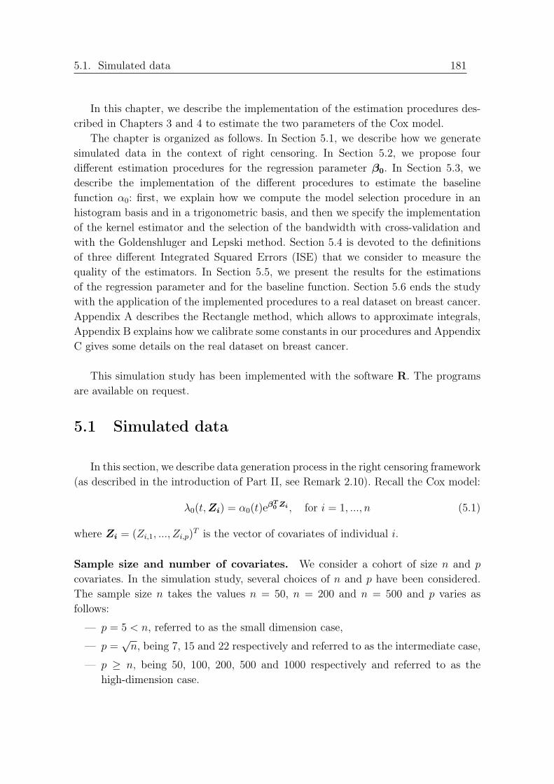
5.1. Simulated data 181
In this chapter, we describe the implementation of the estimation procedures des-cribed in Chapters 3 and 4 to estimate the two parameters of the Cox model.
The chapter is organized as follows. In Section 5.1, we describe how we generatesimulated data in the context of right censoring. In Section 5.2, we propose fourdifferent estimation procedures for the regression parameter β0. In Section 5.3, wedescribe the implementation of the different procedures to estimate the baselinefunction α0: first, we explain how we compute the model selection procedure in anhistogram basis and in a trigonometric basis, and then we specify the implementationof the kernel estimator and the selection of the bandwidth with cross-validation andwith the Goldenshluger and Lepski method. Section 5.4 is devoted to the definitionsof three different Integrated Squared Errors (ISE) that we consider to measure thequality of the estimators. In Section 5.5, we present the results for the estimationsof the regression parameter and for the baseline function. Section 5.6 ends the studywith the application of the implemented procedures to a real dataset on breast cancer.Appendix A describes the Rectangle method, which allows to approximate integrals,Appendix B explains how we calibrate some constants in our procedures and AppendixC gives some details on the real dataset on breast cancer.
This simulation study has been implemented with the software R. The programsare available on request.
5.1 Simulated data
In this section, we describe data generation process in the right censoring framework(as described in the introduction of Part II, see Remark 2.10). Recall the Cox model:
λ0(t,Zi) = α0(t)eβT0Zi , for i = 1, ..., n (5.1)
where Zi = (Zi,1, ..., Zi,p)T is the vector of covariates of individual i.
Sample size and number of covariates. We consider a cohort of size n and p
covariates. In the simulation study, several choices of n and p have been considered.The sample size n takes the values n = 50, n = 200 and n = 500 and p varies asfollows:
— p = 5 < n, referred to as the small dimension case,
— p =√n, being 7, 15 and 22 respectively and referred to as the intermediate case,
— p ≥ n, being 50, 100, 200, 500 and 1000 respectively and referred to as thehigh-dimension case.

182 Chapitre 5. Simulations
Regression parameter in the Cox model. The true regression parameter β0 ischosen as a vector of dimension p, defined by β0 = (0.1, 0.3, 0.5, 0, ..., 0)T ∈ R
p, forvarious p ≥ 3.
Matrix design. For each n and p, the design matrix Z = (Zi,j)1≤i≤n,1≤j≤p is simu-lated independently from a uniform distribution on [−1, 1].
Survival times and baseline function. We consider two forms for the true base-line function α0 depending on the distribution of the survival time.
(i) If the survival times are distributed according to a Weibull distribution W(a, λ),the baseline function is of the form α0(t) = aλata−1, where a and λ are twopositive parameters. From the relation between the conditional survival functionand the conditional hazard rate function, we have for i = 1, ..., n,
S(t,Zi) = exp[−∫ t
0
λ0(s,Zi)ds]= exp(−λataeβ
T0Zi).
We simulate n uniform random variables Yi ∼ U([0, 1]), for i = 1, ..., n. Invertingthe conditional survival function, one gets an explicit expression of the survivaltimes Ti:
Ti =1
λ
(− eβ
T0Zi log(1− Yi)
)1/a.
We implement Ti from this expression. We simulate three Weibull distributionsfor the survival times: W(1.5, 1), W(0.5, 2), W(3, 4).
(ii) If the survival times are distributed according to a log-normal distributionlnN (λ, a), the baseline function is of the form
α0(t) =
1a√2πt
exp(− (log t−λ)2
2a2
)
1− Φ(
log t−λa
) ,
where Φ is the cumulative distribution function of the standard normal distri-bution. The associated survival time Ti is defined for i = 1, ..., n, by
Ti = exp
(aΦ−1
(1− exp
(log(1− Yi)
eβT0Zi
))+ λ
), where Yi ∼ U([0, 1]).
We simulate three log-normal distributions for the survival times: lnN (0.25, 0),lnN (1, 0), lnN (10, 0).
From the different distributions considered, we obtain several different forms for thebaseline hazard function α0 (see Figure 1.0.1).
5.1. Simulated data 183
0.0 0.5 1.0 1.5
01
23
45
grille_temps
alpha01
LogN(1/4,0)
LogN(1,0)
LogN(10,0)
0.0 0.5 1.0 1.5
0.5
1.0
1.5
grille_temps
alpha04
W(1.5,1)
W(0.5,2)
W(3,4)
Figure 1.0.1 – Plots of the baseline hazard function for different parameters of a log-normaldistribution (left) and of a Weibull distribution (right).
Censoring times. We set a rate of censoring of the form 1/γE[T1], where γ > 0 isa constant to be adjusted to the rate of censorship. We consider two different rates ofcensoring:
— a large rate of censoring of 50% by taking γ = 1.2,
— a moderate rate of 20% of censorship by taking γ = 4.5.
The censoring times (Ci)1≤i≤n are simulated independently from the survival times viaan exponential distribution E(1/γE[T1]), with rate parameter 1/γE[T1].
Time interval of the study. The time τ of the end of the study is taken as thequantile at 90% of (Ti ∧ Ci)i=1,...,n. We consider in the following that τ is non-random.A theoretical study with a random τ is beyond the scope of the present study.
Observed times and censoring indicator. For i = 1, ..., n, we compute the obser-ved times Xi = min(Ti, Ci), where Ci = Ci∧τ , and the censoring indicators δi = 1Ti≤Ci
.The definition of Ci ensures that there exist some i ∈ 1, ..., n for which Xi ≥ τ , sothat all estimators are defined on the interval [0, τ ], and it prevents from certain edgeeffect.
Each sample (Zi, Ti, Ci, Xi, δi, i = 1, ..., n) is repeated Ne = 100 times (we consider

184 Chapitre 5. Simulations
Ne = 500 for some experiments but it takes too much time to rise Ne to 500 in eachone).
5.2 Step 1: Estimation of the regression parameter
β0
We implement four procedures to estimate the regression parameter β0: the clas-sical minimization of the opposite of the partial log-likelihood, the classical Lassoprocedure, a procedure that performs a Lasso procedure and a minimization of thepartial log-likelihood on the covariates selected from the Lasso, and lastly the adaptiveLasso procedure. These algorithms are all based on the Cox partial likelihood (2.106),which can be rewritten in the censoring case by
l∗n(β) =1
n
n∑
i=1
δi logeβ
TZi
Sn(Xi,β), where Sn(β, Xi) =
∑
k:Xk≥Xi
eβTZk . (5.2)
Let us describe these four different strategies.
1. The maximum Cox partial log-likelihood estimation: According to (5.2),the maximum Cox partial log-likelihood estimator is defined by
βML
= argmaxβ
l∗n(β)).
This procedure is implemented in R with the coxph function, located in thesurvival library in R (see Andersen & Gill (1982) and Therneau & Grambsch(2000) for theoretical and practical details about this procedure). The obtainedestimator is consistent (see Tsiatis (1981) and Andersen & Gill (1982)) andasymptotically efficient. The maximum Cox partial log-likelihood procedureworks well when the number of covariates p is not too large compared withn. When p increase, the estimations become wrong and when p is really toolarge, the procedure does not converge anymore. In theory, the high-dimensionis reached when p is of order n, but in practice the coxph algorithm can nolonger be used as soon as p exceeds
√n. Thus, we consider the coxph algorithm
only in the cases when p ≤ √n.
2. The Lasso: Recall that the Lasso estimator, introduced by Tibshirani (1997),is defined by
βLasso
µ = argminβ
−l∗n(β) + µ|β|1, (5.3)
where µ > 0 is a regularization parameter.

5.2. Step 1: Estimation of the regression parameter β0 185
The problem (5.3) is convex (see Huang et al. (2013) for example) and imple-mentable. The Lasso procedure for the Cox model has been implemented in Rby Simon et al. (2011) with the glmnet function (located in the glmnet libraryin R). This algorithm is based on a cyclical coordinate descent. The idea is thefollowing: one minimizes on one coordinate a quadratic approximation of theCox partial log-likelihood. This amounts to consider in the hessian only onenon-zero coordinate on the diagonal. We obtain a gradient descent, to which weapply a soft-threshholding operator (associated with the ℓ1 penalty). One doesthis procedure in every directions. As proposed by Tibshirani (1996) and imple-mented in the glmnet procedure, the regularization parameter µ is chosen viacross-validation. The Lasso procedure (5.3) is defined for all p, in particular itis adapted to the case p ≥ n. The resulting estimator is sparse and thus easilyinterpretable.
One limitation of the Lasso procedure is that it is in general biased (see Zhang& Huang (2008a)) and in some case inconsistent for variable selection (see Zou(2006)). To overcome these problems, we consider two other procedures (seeParagraph 3 for a procedure that corrects the bias of the Lasso and Paragraph4 for a procedure that provides a consistent estimator).
3. A Lasso associated to a maximum Cox partial log-likelihood estima-
tion: In order to correct the bias of the Lasso procedure, we propose a two-stepestimation procedure, which combines the two previous procedures. First, weselect the non-zero coordinates of β0 with the glmnet procedure, we obtain theLasso estimator β. Second, to the Cox model with those selected variables, weapply a coxph procedure. To be more precise, let define the sparsity set of β byJ(β) = j ∈ 1, ..., p : βj 6= 0 and its sparsity index by |J(β)| = Card J(β).Let also consider Z the vector of covariates such that Zj = Zj when j ∈ J(β)
and Zj = 0 otherwise. The resulting estimator is then defined by
βLasso+ML
= argminβ∈R|J(β)|
−l∗n(β),
where
l∗n(β) =1
n
n∑
i=1
δi logeβ
T Zi
Sn(Xi,β)and Sn(Xi,β) =
∑
k:Xk≥Xi
eβT Zk .
This procedure is not always defined. Indeed, when the number of selectedcovariates with the Lasso procedure is still too large (i.e. larger than
√n), the
minimization of the opposite of the Cox partial log-likelihood is not possible. Inthis case, we only consider a Lasso procedure, without adding the second stepwith the coxph procedure.
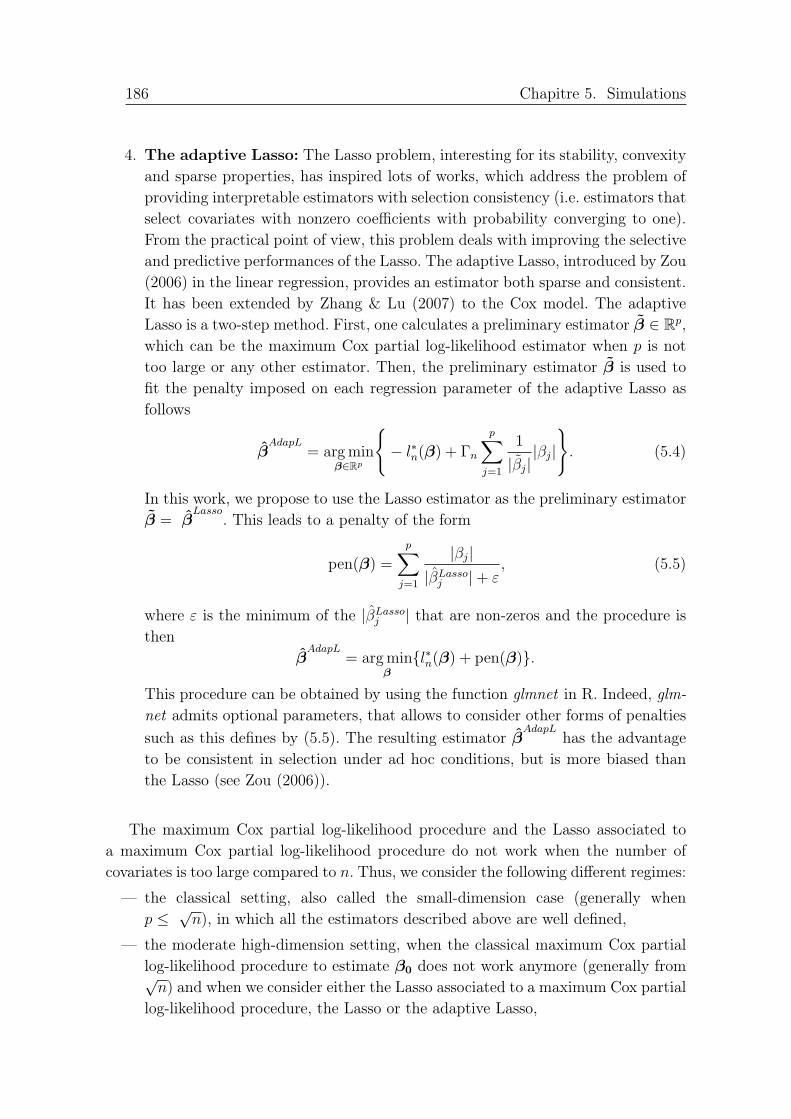
186 Chapitre 5. Simulations
4. The adaptive Lasso: The Lasso problem, interesting for its stability, convexityand sparse properties, has inspired lots of works, which address the problem ofproviding interpretable estimators with selection consistency (i.e. estimators thatselect covariates with nonzero coefficients with probability converging to one).From the practical point of view, this problem deals with improving the selectiveand predictive performances of the Lasso. The adaptive Lasso, introduced by Zou(2006) in the linear regression, provides an estimator both sparse and consistent.It has been extended by Zhang & Lu (2007) to the Cox model. The adaptiveLasso is a two-step method. First, one calculates a preliminary estimator β ∈ R
p,which can be the maximum Cox partial log-likelihood estimator when p is nottoo large or any other estimator. Then, the preliminary estimator β is used tofit the penalty imposed on each regression parameter of the adaptive Lasso asfollows
βAdapL
= argminβ∈Rp
− l∗n(β) + Γn
p∑
j=1
1
|βj||βj|. (5.4)
In this work, we propose to use the Lasso estimator as the preliminary estimatorβ = β
Lasso. This leads to a penalty of the form
pen(β) =
p∑
j=1
|βj||βLasso
j |+ ε, (5.5)
where ε is the minimum of the |βLassoj | that are non-zeros and the procedure is
thenβ
AdapL= argmin
β
l∗n(β) + pen(β).
This procedure can be obtained by using the function glmnet in R. Indeed, glm-
net admits optional parameters, that allows to consider other forms of penalties
such as this defines by (5.5). The resulting estimator βAdapL
has the advantageto be consistent in selection under ad hoc conditions, but is more biased thanthe Lasso (see Zou (2006)).
The maximum Cox partial log-likelihood procedure and the Lasso associated toa maximum Cox partial log-likelihood procedure do not work when the number ofcovariates is too large compared to n. Thus, we consider the following different regimes:
— the classical setting, also called the small-dimension case (generally whenp ≤ √
n), in which all the estimators described above are well defined,
— the moderate high-dimension setting, when the classical maximum Cox partiallog-likelihood procedure to estimate β0 does not work anymore (generally from√n) and when we consider either the Lasso associated to a maximum Cox partial
log-likelihood procedure, the Lasso or the adaptive Lasso,

5.3. Step 2: Estimation of the baseline function α0 187
— the high-dimensional setting, when p ≥ n, for which only the Lasso and theadaptive Lasso work.
Even without reaching the ultra high-dimension, as defined by Verzelen (2012), thealgorithms, such as the Lasso or the adaptive Lasso, are performing poorly whenp ≫ n. In this case, one proceeds to a preliminary screening to reduce the number ofcovariates to be entered in the multivariate model (see Section 5.6 for details on thescreening and application to a real dataset on breast cancer). Generally, one attemptsto obtain a p of order n.
5.3 Step 2: Estimation of the baseline function α0
We now describe the implementation of the two strategies to estimate the baselinehazard function: the model selection and the kernel estimation. We implement themodel selection in two different bases of functions and for the kernel estimation, weimplement two procedures to select the bandwidth. The resulting estimators are thefollowing:
1. The penalized contrast estimator αβ
mβobtained by model selection, in
(i) Histogram basis
(ii) Trigonometric basis
2. The kernel estimator with a bandwidth selected by
(i) Cross-validation,
(ii) The Goldenshluger and Lepski method,
the resulting estimators are denoted by αβ
hβCV
and αβ
hβrespectively.
Note that all the three estimators of the baseline function depends on the estimatorβ implemented in the first step. Let us precise how we implement all the procedures.
5.3.1 Penalized contrast estimator and model selection
We refer to Chapter 3 for a detailed description of the procedure and briefly recallit.
The model selection method is based on the minimization of a contrast. Thiscontrast in our context is defined for a function α ∈ (L2 ∩ L
∞)([0, τ ]) by
Cn(α, β) = − 2
n
n∑
i=1
α(Xi)δi +1
n
n∑
i=1
∫ Xi
0
α2(t)eβTZidt. (5.6)
Let Mn be a set of indices and Sm,m ∈ Mn be a collection of models:
Sm = α : α(t) =∑
j∈Jm
amj ϕmj (t), a
mj ∈ R,

188 Chapitre 5. Simulations
where (ϕmj )j∈Jm is an orthonormal basis of (L2∩L
∞)([0, τ ]) for the usual L2(P )- norm.We denote Dm the cardinality of Sm, i.e. |Jm| = Dm. From Assumption 3.1.(i), onemust have Dm ≤ √
n/ log n for all m ∈ Mn. Associated to the collection of models,we define the sequence of minimum contrast estimators (αβ
m)m∈Mnwith
αβm = argmin
α∈Sm
Cn(α, β).
The relevant space is automatically selected by using following penalized criterion
mβ = argminm∈Mn
Cn(αβm, β) + pen(m), (5.7)
with
pen(m) := κ(1 + ||α0||∞,τ )Dm
n, (5.8)
The penalized contrast estimator is then αβ
mβ.
Implementation of the minimum contrast estimators αβm
By definition, for m ∈ Mn, αβm belongs to the model Sm. Thus, there exists
Aβm
= (aβj )j∈Jm such that, for (ϕmj )j∈Jm an orthonormal basis of (L2 ∩ L
∞)([0, τ ])
andαβm(t) =
∑
j∈Jm
aβj ϕmj (t), ∀t ∈ [0, τ ] (5.9)
is the solution of the equation
GβmAβ
m= Γm, (5.10)
where Gβm
and Γm are respectively defined by
Gβm
=( 1n
n∑
i=1
∫ Xi
0
ϕj(t)ϕk(t)eβTZiYi(t)dt
)(j,k)∈J2
m
, (5.11)
Γm =( 1n
n∑
i=1
δiϕj(Xi))j∈Jm
. (5.12)
We implement αβm in two different bases of (L2 ∩ L
∞)([0, τ ]): the histogram basis andthe trigonometric basis, both described in Chapter 3, Example 3.1.
(i) Histogram basis (see Chapter 3, Example 3.1.1.). In this case,
ϕmj (t) =
1√τ2m/2
1[(j−1)τ
2m, jτ2m
)(t), for j = 1, ..., 2m,

5.3. Step 2: Estimation of the baseline function α0 189
such that Dm = 2m ≤ √n/ log n, according to Assumption 3.1.(i). We take in
the program m = 0, ..., ⌊log(n/ log(n))/ log(2))⌋. The solution of Equation (5.10)satisfies
aβj =τ
2m1
1n
n∑
i=1
eβTZi
((min
(Xi,
jτ
2m
)− (j − 1)τ
2m
)∨ 0)1
n
n∑
i=1
δi2m/2
√τ1[
(j−1)τ2m
, jτ2m
)(Xi).
(5.13)
For m = 0, ..., ⌊log(n/ log(n))/ log(2))⌋, we compute the candidates αβm for the
estimation of α0 using relation (5.9).
(ii) Trigonometric basis (see Chapter 3, Example 3.1.2.). Recall that
ϕ1(t) =√
2/τ ,
ϕ2j(t) =√
2/τ cos(2πjt/τ), for j ≥ 1,
ϕ2j+1(t) =√
2/τ sin(2πjt/τ), for j ≥ 1.
For this model, Dm = m ≤ √n/log n according to Assumption 3.1.(i). In the
program, we add two models by taking m = 1, ..., ⌊√n/ log(n) + 2⌋. In practice,it is classic to consider more models than what the theory authorizes (see Brunelet al. (2010) for example). Then, to solve Equation (5.10), we compute the Grammatrix Gβ
mand the vector Γm by calculating the integrals defined in (5.11) and
(5.12) for all possibilities: let q 6= r in N∗,
(Gβm)1,1 =
1
nτ
n∑
i=1
eβTZiXi,
(Gβm)1,2q =
√2
n
n∑
i=1
eβTZi
sin(2πqXi/τ)
2πq,
(Gβm)1,2q+1 =
√2
n
n∑
i=1
eβTZi
(1
2πq− cos(2πqXi/τ)
2πq
),
(Gβm)2q,2q =
2
n
n∑
i=1
eβTZi
(cos(2πqXi/τ) sin(2πqXi/τ)
4πq+
Xi
2τ
),
(Gβm)2q+1,2q+1 =
2
n
n∑
i=1
eβTZi
(Xi
2τ− cos(2πqXi/τ) sin(2πqXi/τ)
4πq
),
(Gβm)2q+1,2r+1 =
2
n
n∑
i=1
eβTZi
(sin(2π(q − r)Xi/τ)
4π(q − r)− sin(2π(q + r)Xi/τ)
4π(q + r)
),
(Gβm)2q,2r =
2
n
n∑
i=1
eβTZi
(sin(2π(q + r)Xi/τ)
4π(q + r)+
sin(2π(q − r)Xi/τ)
4π(q − r)
),
190 Chapitre 5. Simulations
(Gβm)2q+1,2r =
2
n
n∑
i=1
eβTZi
(sin2(π(q + r)Xi/τ)
2π(q + r)+
sin2(π(q − r)Xi/τ)
2π(q − r)
),
(Gβm)2q+1,2q =
2
n
n∑
i=1
eβTZi
sin2(2πqXi/τ)
4πq,
and
(Γm)1 =1
n√τ
n∑
i=1
1Xi≤τ,δi=1,
(Γm)2q =1
n
√2
τ
n∑
i=1
δi cos(2πqXi), (Γm)2q+1 =1
n
√2
τ
n∑
i=1
δi sin(2πqXi).
From these relations, we get the Gram matrix Gβm
and the vector Γm,so that Equation (5.10) can be solve by inverting Gβ
m. Thus, for each
m ∈ 0, ..., ⌊√n/ log(n) + 2⌋, we obtain a solution Aβm
and the candidatesαβm for the estimation of α0 are implemented by using relation (5.9).
Implementation of the model selection procedure
The estimator of the baseline function α0 is obtained via the model selection pro-cedure (5.7), where Mn = 1, ..., ⌊log(n/ log(n))/ log(2))⌋ in the histogram case andMn = 1, ..., ⌊√n/ log(n)+2⌋ in the trigonometric case. The contrast is implementedfrom definition (5.6). Applying the rectangle method (see Appendix A for details onthis method), the contrast (5.6) is approximated by
Cn(αβm, β) ≈ − 2
n
n∑
i=1
αβm(Xi)δi +
1
n
n∑
i=1
eβTZi
∑
j:uj≤Xi
(αβm(uj))
2 τ
N,
where N = 100, and (uj)j=1,...,N are grid points evenly distributed across [0, τ ].The penalty defined in Equation (5.8) involves the unknown quantity ||α0||∞,τ . This
problem occurs occasionally in penalization procedures, see for instance Comte (2001),Lacour (2007) or Comte et al. (2011). The solution is to replace it by an estimator:
pen(m) = κ(1 + ||αβ
max(m)||∞,τ )Dm
n, (5.14)
where κ is a numerical constant and αβ
max(m) is an estimator of α0 computed on thearbitrary larger space Smax(m). The constant κ in the penalty term is a universalnumerical constant. From several tests, the constant κ is tuned to κ = 5. We refer toAppendix B for the details on the procedure to choose κ.
We compute mβ from (5.7) and the resulting estimator is αβ
mβ, β being alternately
βML
, βLasso
, βLasso+ML
, βAdapL
.

5.3. Step 2: Estimation of the baseline function α0 191
5.3.2 Kernel estimators and bandwidth selection
Implementation of the kernel estimator αβh
Let recall the definition of the usual kernel estimator of the baseline function,introduced by Ramlau-Hansen (1983b), in the specific case of right censoring: for akernel function K : R 7→ R with integral 1 and a bandwidth h > 0,
αβh (t) =
1
h
n∑
i=1
δi∑nk=1 e
βTZk1Xk≥XiK
(t−Xi
h
). (5.15)
Among the classical kernel function used in kernel estimation, we choose to work withthe Epanechnikov kernel, defined by
K(u) =3
4(1− u2)1|u|≤1.
Estimator (5.15) has been calculated for β being alternately βML
, βLasso
, βLasso+ML
,
βAdapL
.
Implementation of the bandwidth selection
We propose two data-driven procedures to select the bandwidth: the cross-validation and the Goldenshluger and Lepski method.
(i) Implementation of the cross-validation
Cross-validation is a popular and readily implemented heuristic for selectingthe bandwidth in kernel estimation. The cross-validation method for the multi-plicative intensity model for counting processes has been suggested by Ramlau-Hansen (1981). The cross-validated bandwidth is chosen to minimize an estimateof the Mean Integrated Squared Error (MISE) as a function of h, and defined by
MISE(h) = E
∫ τ
0
(αβh (t))
2dt− 2E
∫ τ
0
αβh (t)α0(t)dt+
∫ τ
0
α20(t)dt
The last term does not depend on h and the first term is estimated accordingto (5.15). Ramlau-Hansen (1981) showed that an approximatively unbiased es-timator of the second term is the "cross-validation" estimate
−2∑
i 6=j
1
hK(Xi −Xj
h
)∆N(Xi)
Y (Xi)
∆N(Xj)
Y (Xj),
where the sum is over i and j such that i 6= j and 0 ≤ Xi ≤ τ and Y =∑ni=1 1Xi≥t. In this case, the bandwidth selected by cross-validation is
hβCV = argmin
h
E
∫ τ
0
(αβh (t))
2dt− 2∑
i 6=j
1
hK(Xi −Xj
h
)∆N(Xi)
Y (Xi)
∆N(Xj)
Y (Xj)
.

192 Chapitre 5. Simulations
(ii) Implementation of the Goldenshluger and Lepski method
In this paragraph, we describe the implementation of the adaptive Goldenshlugerand Lepski method (described in Chapter 4) to select an adaptive bandwidth forthe kernel estimator (5.15).
Let us recall few outlines of the Goldenshluger and Lepski method. For Hn adiscrete set of bandwidths specified in the following, we have for h > 0
Aβ(h) = suph′∈Hn
||αβ
h,h′ − αβh′ ||22 − V (h′)
+,
where
V (h) = κ′ ||α0||∞,τ ||K||22nh
, (5.16)
for some numerical constant κ′ > 0 to be specified later, and
αβh,h′(t) = Kh′ ∗ αβ
h (t), (5.17)
for any t ≥ 0 and h, h′ two positive real numbers. From these definitions, theselected bandwidth is:
hβ = argminh∈Hn
Aβ(h) + V (h),
and the resulting kernel estimator is denoted αβ
hβ.
In order to implement the adaptive bandwidth selection method, we consider agrid of bandwidths Hn defined by
Hn = 1/2k, k = 0, ..., ⌊log(n)/ log(2)⌋.
This grid satisfies the theoretical conditions required to establish the non-asymptotic oracle inequality (see Example 4.1 in Chapter 4). The auxiliary esti-
mates αβh,h′ defined by (5.17) are easily computed by the rectangle method (see
Appendix A for details about this approximation method):
αβh,h′(t) ≈
N∑
j=1
Kh′(t− uj)αβh (uj)
τ
N,
and the standard L2-norm in Aβ(h) is then approximate by
||αβh,h′ − αβ
h′ ||22 ≈N∑
kj=1
(αβh,h′(uj)− αβ
h′(uj))2 τ
N,
where N = 100, and (uj)j are grid points evenly distributed across [0, τ ].

5.4. Measuring the quality of the estimators 193
The variance term V (h) defined by (5.16) involves the unknown quantity||α0||∞,τ . Following Bouaziz et al. (2013), we propose to replace the true unknownfunction by an estimator and to consider rather:
V β(h) = κ′ ||αβ
max(h)||∞,τ ||K||22nh
, (5.18)
where κ′ is a numerical constant and αβ
max(h) an estimator computed for thelargest bandwidth h in the grid Hn. The constant κ′ is a universal constant thatwe tuned from different tests detailed in Appendix B.We take κ′ = 1.
Finally, we select hβ such that
hβ = argminh∈Hn
Aβ(h) + V β(h). (5.19)
We compute αβ
hβfrom (5.15) and (5.19).
5.4 Measuring the quality of the estimators
The performances of the different estimators of the baseline hazard function andof the complete hazard function are evaluated via Mean Integrated Squared errors(MISEs). Let first define the three Integrated Squared Errors (ISEs) considered forsome function α ∈ L
2([0, τ ]) and some parameter β ∈ Rp: the standard ISE, the
random ISE more adapted to the Cox model and the total ISE are respectively definedby
ISEstand(α) =
∫ τ
0
(α(t)− α0(t))2dt,
ISErand(α,β) =1
n
n∑
i=1
∫ Xi
0
(α(t)− α0(t))2eβ
TZidt, (5.20)
ISEtotal(α,β) =1
n
n∑
i=1
∫ τ
0
(α(t)eβTZi − α0(t)e
βT0Zi)2dt.
Remark 5.1. In Chapter 3, we have introduced a random norm defined by (3.17) inSection 3.2. This explain why we introduce the ISErand which is inspired by the ran-dom norm. In addition the ISErand is more adapted to Cox model than the standardISE. We also introduce the ISEtotal to measure the quadratic error of the estimatorλ(t,Zi) = αβ(t)eβ
TZi of the whole intensity λ0 in the Cox model, for αβ being either
αβ
hβCV
, αβ
mβor αβ
hβ. It is close to the quadratic norm considered in Chapter 2.
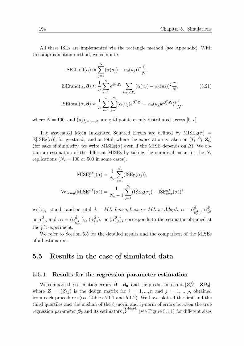
194 Chapitre 5. Simulations
All these ISEs are implemented via the rectangle method (see Appendix). Withthis approximation method, we compute:
ISEstand(α) ≈N∑
j=1
(α(uj)− α0(uj))2 τ
N,
ISErand(α,β) ≈ 1
n
n∑
i=1
eβTZi
∑
j:uj≤Xi
(α(uj)− α0(uj))2 τ
N, (5.21)
ISEtotal(α,β) ≈ 1
n
n∑
i=1
N∑
j=1
(α(uj)eβTZi − α0(uj)e
βT0Zi)2
τ
N,
where N = 100, and (uj)j=1,...,N are grid points evenly distributed across [0, τ ].
The associated Mean Integrated Squared Errors are defined by MISEg(α) =
E[ISEg(α)], for g=stand, rand or total, where the expectation is taken on (Ti, Ci,Zi)
(for sake of simplicity, we write MISEg(α) even if the MISE depends on β). We ob-tain an estimation of the different MISEs by taking the empirical mean for the Ne
replications (Ne = 100 or 500 in some cases).
MISEg,kemp(α) =
1
Ne
Ne∑
j=1
(ISEg(αj)),
Varemp(MISEg,k(α)) =1
Ne − 1
Ne∑
j=1
(ISEg(αj)− ISEg,kemp(α))
2
with g=stand, rand or total, k = ML,Lasso, Lasso +ML or AdapL, α = αβ
hβCV
, αβ
hβ
or αβ
mβand αj = (αβ
hβCV
)j, (αβ
hβ)j or (αβ
mβ)j corresponds to the estimator obtained at
the jth experiment.We refer to Section 5.5 for the detailed results and the comparison of the MISEs
of all estimators.
5.5 Results in the case of simulated data
5.5.1 Results for the regression parameter estimation
We compare the estimation errors |β−β0| and the prediction errors |Zβ−Zβ0|,where Z = (Zi,j) is the design matrix for i = 1, ..., n and j = 1, ..., p, obtainedfrom each procedures (see Tables 5.1.1 and 5.1.2). We have plotted the first and thethird quartiles and the median of the ℓ1-norm and ℓ2-norm of errors between the true
regression parameter β0 and its estimators βAdapL
(see Figure 5.1.1) for different sizes

5.5. Results in the case of simulated data 195
of n and p. All the regimes are represented : the small dimension for p = 5, theintermediate case for p =
√n and the high-dimension for p = n or p = 2n.
ML Lasso AdapL
n = 200 p = 5|β − β0|1 0.586 0.502 0.508
|β − β0|2 0.115 0.103 0.116
n = 500 p = 5|β − β0|1 0.359 0.324 0.306
|β − β0|2 0.043 0.043 0.042
ML Lasso AdapL
n = 200 p = 15|β − β0|1 1.750 0.690 0.818
|β − β0|2 0.353 0.149 0.216
n = 500 p = 22|β − β0|1 1.67 0.556 0.692
|β − β0|2 0.203 0.072 0.112
ML Lasso AdapL
n = 200 p = 200|β − β0|1 NA 0.984 1.62
|β − β0|2 NA 0.276 0.541
n = 500 p = 500|β − β0|1 NA 0.808 1.67
|β − β0|2 NA 0.161 0.361
Table 5.1.1 – ℓ1-norm and ℓ2 norm of estimation errors of the estimators βML
, βLasso
and
βAdapL
for n = 200 and p = 5, 15, 200, and n = 500 and p = 5, 22, 500.
Comments on Table 5.1.1, Table 5.1.2 and Figure 5.1.1.
On Figure 5.1.1, we plot the three quartiles (the first and the third quartiles repre-sented by a cross (×) and the median represented by a bullet (•)) of the ℓ1-norm (onthe left) and the ℓ2-norm (on the right) of the estimation errors for the maximum Coxpartial log-likelihood estimator (see 5.1.1a and 5.1.1b), for the Lasso estimator (see5.1.1c and 5.1.1d) and for the adaptive Lasso estimator (see 5.1.1e and 5.1.1e) of theregression parameter β0 for different values of n and p. In blue, we plot the quartiles ofthe estimation errors of the three estimators for n = 50 and p = 5, p = 7, p = 100; thered color corresponds to the quartiles of the estimation errors of the three estimatorsfor n = 200 and p = 5, p = 15, p = 500; the green color corresponds to the quartiles ofthe estimation errors of the three estimators for n = 500 and p = 5, p = 22, p = 1000.The dotted lines just help in interpreting the trends in the graphs.
As expected, we observe that the larger the sample size n is, the smaller the ℓ1-norm and ℓ2-norm of the estimation and prediction errors of the estimators of β0 are;and inversely the higher the number of covariates is, the greater the estimation andprediction errors of the estimators of β0 are. The maximum Cox partial log-likelihoodestimator β
MLis not defined for p >
√n. From Tables 5.1.1 and 5.1.2, it seems that
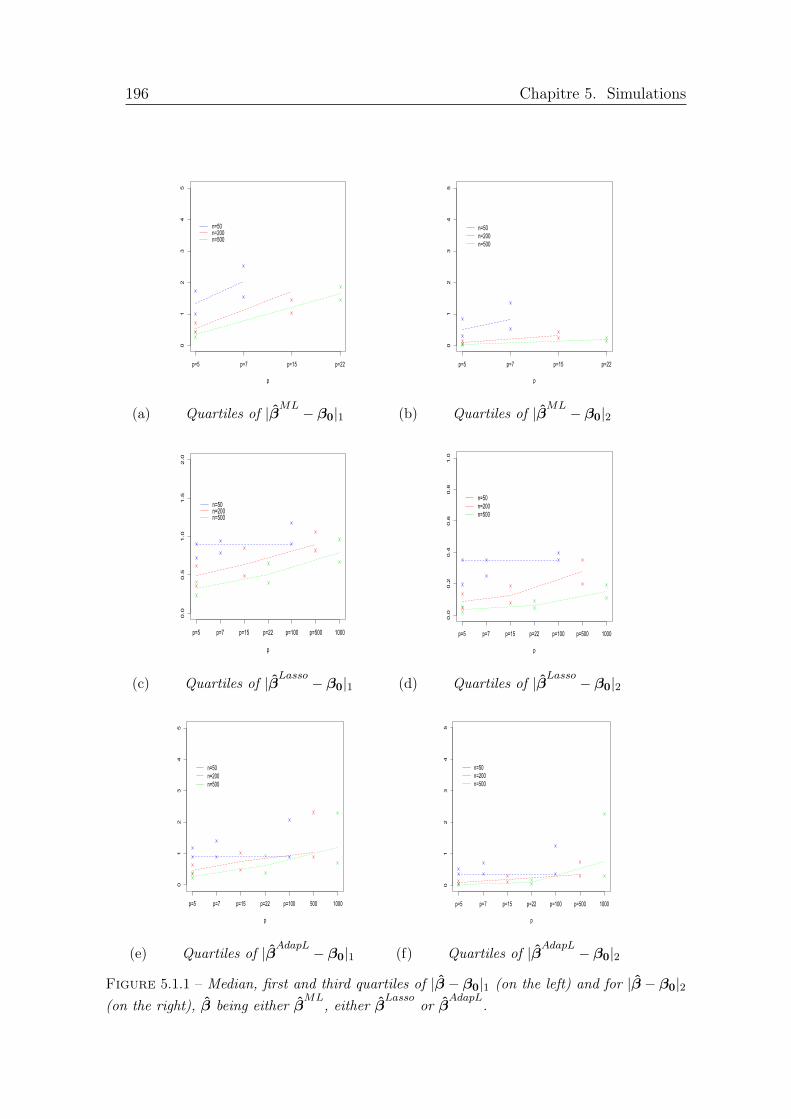
196 Chapitre 5. Simulations
01
23
45
p
p=5 p=7 p=15 p=22
n=50
n=200
n=500
(a) Quartiles of |βML − β0|1
01
23
45
p
p=5 p=7 p=15 p=22
n=50
n=200
n=500
(b) Quartiles of |βML − β0|2
0.0
0.5
1.0
1.5
2.0
p
p=5 p=7 p=15 p=22 p=100 p=500 1000
n=50n=200n=500
(c) Quartiles of |βLasso − β0|1
0.0
0.2
0.4
0.6
0.8
1.0
p
p=5 p=7 p=15 p=22 p=100 p=500 1000
n=50
n=200
n=500
(d) Quartiles of |βLasso − β0|2
01
23
45
p
p=5 p=7 p=15 p=22 p=100 500 1000
n=50
n=200
n=500
(e) Quartiles of |βAdapL − β0|1
01
23
45
p
p=5 p=7 p=15 p=22 p=100 p=500 1000
n=50
n=200
n=500
(f) Quartiles of |βAdapL − β0|2
Figure 5.1.1 – Median, first and third quartiles of |β − β0|1 (on the left) and for |β − β0|2(on the right), β being either β
ML, either β
Lassoor β
AdapL.

5.5. Results in the case of simulated data 197
ML Lasso AdapL
n = 200 p = 5|Zβ −Zβ0|1 0.148 0.139 0.146
|Zβ −Zβ0|2 0.036 0.033 0.036
n = 500 p = 5|Zβ −Zβ0|1 0.090 0.088 0.087
|Zβ −Zβ0|2 0.013 0.013 0.013
ML Lasso AdapL
n = 200 p = 15|Zβ −Zβ0|1 0.259 0.170 0.200
|Zβ −Zβ0|2 0.108 0.047 0.069
n = 500 p = 22|Zβ −Zβ0|1 0.200 0.118 0.144
|Zβ −Zβ0|2 0.063 0.022 0.036
ML Lasso AdapL
n = 200 p = 200|Zβ −Zβ0|1 NA 0.231 0.315
|Zβ −Zβ0|2 NA 0.083 0.181
n = 500 p = 500|Zβ −Zβ0|1 NA 0.170 0.255
|Zβ −Zβ0|2 NA 0.046 0.118
Table 5.1.2 – ℓ1-norm and ℓ2 norm of prediction errors of the estimators βML
, βLasso
and
βAdapL
for n = 200 and p = 5, 15, 200, and n = 500 and p = 5, 22, 500.
the Lasso performs better than the Adaptive Lasso in estimation and in prediction.The reason for this is that the adaptive Lasso estimator is more biased than theLasso estimator. However, the adaptive Lasso performs better in selection since it setsmore coefficients to zero. In order to explain this effect more precisely, we computespecificities (SPEC) and sensitivities (SENS) for each method for n = 200 and p = 200.For an estimation βm, the false (FP) and true (TP) positives are defined as
FP(βm) = Card(j ∈ 1, ..., p : βmj
6= 0 and β0j = 0)
TP(βm) = Card(j ∈ 1, ..., p : βmj
6= 0 and β0j 6= 0)
and false (FN) and true (TN) negatives are defined by exchanging = and 6= in theabove definitions. The specificity and sensibility of a method are defined over theNe = 50 replications as
SPEC =1
Ne
Ne∑
m=1
TN(βm)
TN(βm) + FP(βm)
SENS =1
Ne
Ne∑
m=1
TP(βm)
TP(βm) + FN(βm).
From Table 5.1.3, the adaptive Lasso has the best specificity, but has a lower sensitivitythan the Lasso. This is a consequence of the fact that the adaptive Lasso sets morecoefficients to zero.

198 Chapitre 5. Simulations
SPEC SENSLasso 0.97 0.36AdapL 0.98 0.35
Table 5.1.3 – Specificities (SPEC) and sensitivities (SENS) for the Lasso and the adaptiveLasso (AdapL) for n = 200 and p = 200.
We would have also expected that the maximum Cox partial likelihood estimatorperforms better than Lasso estimator when p is small, but it does not. This can beenexplained from the calculation of the ℓ1-norm of the estimation error on the supportof β0, defined by J(β0) = j ∈ 1, ..., p : β0j 6= 0, and on its complementary J(β0)
c.
|(β − β0)J(β0)|1 |(β − β0)J(β0)c |1ML 0.36 1.37
Lasso 0.53 0.21
Table 5.1.4 – ℓ1-norm of the estimation errors on the support of β0 and its complementaryfor the maximum Cox partial likelihood and the Lasso estimators for n = 200 and p = 15.
From Table 5.1.4, it follows that the maximum Cox partial likelihood estimatoris better than the Lasso estimator on the support of β0, but since the maximumCox partial likelihood estimator sets no coefficient to zero, its estimation error onthe complementary of the support of β0 is much higher than the one of the Lassoestimator. This explains why the estimation errors in Table 5.1.1 are better for theLasso estimator than for the maximum Cox partial likelihood estimator.
5.5.2 Results for the baseline function estimation
Comments on Figure 5.2.1.
Figure 5.2.1 represents in the case of a log-normal distribution lnN (1/4, 0), the plotsof the true baseline function α0, the kernel estimator with a bandwidth selected bycross-validation, the kernel estimator with a bandwidth selected by the Goldenshlugerand Lepski method and the penalized contrast estimator in a histogram basis (seeFigure 5.2.1a) and in a trigonometric basis (see Figure 5.2.1b).
First of all, Figure 5.2.1 shows that all procedures seems to estimate suitablythe true function (in red). The curves of the kernel estimators with a bandwidthselected by cross-validation and by Goldenshluger and Lepski are close to each other.The penalized contrast estimator seems to have comparable performances to thoseof the two other estimators for small t, but performs less well after t = 0.8. Thisis probably related to the chosen bases and form of the true function. Indeed, thepenalized contrast estimator in a histogram basis is a piecewise function whereas thetrue function to be estimated is continuous and the form of the penalized contrastestimator in a trigonometric basis does not fit exactly the true function α0 because ofthe periodicity of the basis. We confirm these first visual impressions by comparingthe different MISEs of these estimators.

5.5. Results in the case of simulated data 199
0.0 0.2 0.4 0.6 0.8 1.0 1.2 1.4
01
23
45
grille_temps
alpha0
alpha0alpha_mod_histalpha_noyalpha_noy_adap
(a) Histogram basis.
0.0 0.2 0.4 0.6 0.8 1.0 1.2 1.4
01
23
45
grille_temps
alpha0
alpha0alpha_mod_trigalpha_noyalpha_noy_adap
(b) Trigonometric basis.
Figure 5.2.1 – Plots of the true baseline function (in red), the cross-validated kernel estimator(in green), the penalized contrast estimator (in blue) and the adaptive kernel estimator (inblack). The plots have been obtain for: n = 500, p = ⌊√n⌋, α0 ∼ lnN (1/4, 0), d = 4.5
Comments on Figure 5.2.2.
On Figure 5.2.2, we plot the three quartiles (the first and the third quartiles repre-sented by a cross (×) and the median represented by a bullet (•)) of the empiricalrandom MISEs of the kernel estimators with a bandwidth selected either by cross-validation or by the Goldenshluger and Lepski method, and of the penalized contrastestimator in a histogram basis and in a trigonometric basis of the true baseline func-tion in the case of a Weibull distribution W(1.5, 1) for different values of n and p. Inblue, we plot the quartiles of the MISErands of the four estimators for n = 50 andp = 5, p = 7 and p = 100; the red color corresponds to the quartiles of the MISErandsof the four estimators for n = 200 and p = 5, p = 15 and p = 500; the green colorcorresponds to the quartiles of the MISErands of the four estimators for n = 500 andp = 5, p = 22 and p = 1000. The dotted lines just help in interpreting the graphs.
As expected, the random empirical MISEs are smaller, when the sample sizeincreases, and are degraded when the number of covariates p increases. In additions,it seems that the two kernel estimators perform better than the penalized contrastestimators. The kernel estimator with a bandwidth selected by the Goldenshluger andLepski method seems to have the smallest MISEs for all n and p, and the penalizedcontrast estimator in a trigonometric basis the worst.

200 Chapitre 5. Simulations
0.00
0.05
0.10
0.15
0.20
0.25
0.30
0.35
p
p=5 p=7 p=15 p=22 p=100 p=500 1000
n=50
n=200
n=500
(a) MISErand(αβ
AdapL
hβAdapL
CV
).
0.00
0.05
0.10
0.15
0.20
0.25
p
p=5 p=7 p=15 p=22 p=100 p=500 1000
n=50
n=200
n=500
(b) MISErand(αβ
AdapL
hβAdapL
).
0.00
0.05
0.10
0.15
0.20
0.25
0.30
0.35
p
p=5 p=7 p=15 p=22 p=100 p=500 1000
n=50
n=200
n=500
(c) MISErand(αβ
AdapL
mβAdapL
)in the case of
histograms.
0.00
0.05
0.10
0.15
0.20
0.25
p
p=5 p=7 p=15 p=22 p=100 p=500 1000
n=50
n=200
n=500
(d) MISErand(αβ
AdapL
mβAdapL
)in the trigono-
metric case.
Figure 5.2.2 – Median, first and third quartiles of the random MISEs of the kernel estimatorwith a bandwidth selected by cross-validation (5.2.2a), of the kernel estimator with a bandwidthselected by the Goldenshluger and Lepski method (5.2.2b), of the penalized contrast estimatorin the case of histograms (5.2.2c) and of the penalized contrast estimator in the trigonometriccase (5.2.2d), with the adaptive Lasso estimator of the regression parameter in the case of aWeibull distribution W(1.5, 1).

5.5. Results in the case of simulated data 201
Comments on Table 5.2.1.
Table 5.2.1 gives the three empirical MISEs of the kernel estimator with a band-width selected by the Goldenshluger and Lepski method and of the penalized contrastestimator in a histogram basis for an adaptive Lasso estimator of the regression pa-rameter and survival times that are distributed from W(1.5, 1), in different censoringsituation. We consider the results for two rates of censoring: a usual rate of 20% ofcensoring and large rate of 50% of censoring.
For a fixed censure, the better results (i.e the smallest values) are obtained forthe random MISE and the worst results for the total MISE, which seems consistent,since the total MISE measures the performances of the complete intensity estimators,whereas the two other MISEs measures the performances of the estimators of thebaseline function.
Intuitively, one would expect that the MISEs would be degraded when the censoringrate increases. This is not what we observe on Table 5.2.1. The reason for this is thatthe time interval of the study [0, τ ] is smaller for a large rate of censoring. Indeed, thetime τ is the quantile to 90% of the observed times (Xi)i=1,...,n. We calculate its valueon one experiment, we obtain τ1 = 1.48 for 20% of censoring and τ2 = 1.19 for 50% ofcensoring. More precisely, if we take the example of the standard ISE, we have
ISE20%(α) =
∫ τ1
0
(α(t)− α0(t))2dt for 20% of censoring,
ISE50%(α) =
∫ τ2
0
(α(t)− α0(t))2dt for 50% of censoring.
Thus, the ISE for 20% of censoring is obtained from the one of 50% by adding∫ τ1
τ2
(α(t)− α0(t))2dt.
This explains why the MISEs obtained for a higher rate of censoring seem better. Inorder to compare the MISEs in different censoring situations, we could have calculatethe MISEs on the same time interval.
In most cases, the results are better for the kernel estimator with a bandwidthselected by the Goldenshluger and Lepski method than for the penalized contrast esti-mator in a histogram basis, unless for the total empirical MISEs in a high-dimensionalsetting (n = 200 and p = 500), i.e. when we consider the estimator of the completeintensity λ(t,Z) = αβ(t)eβ
TZ .

202
Cha
pitr
e5.
Sim
ulat
ions
❵❵❵❵❵❵❵❵❵❵
❵❵
❵❵❵
DimensionsMISEs
20% 50%
MISEstand MISErand MISEtot MISEstand MISErand MISEtot
n = 200p = 15 0.069 0.018 0.442 0.05 0.01 0.45p = 500 0.44 0.07 7.35 0.33 0.053 9.01
n = 500p = 22 0.03 0.009 0.20 0.022 0.006 0.16p = 1000 0.13 0.02 1.38 0.02 0.004 0.10
(a) MISEs of the kernel estimator of the baseline function with a bandwidth selected by the Goldenshluger andLepski method and an adaptive Lasso estimator of the regression parameter.
❵❵❵❵❵❵❵❵❵❵
❵❵
❵❵❵
DimensionsMISEs
20% 50%
MISEstand MISErand MISEtot MISEstand MISErand MISEtot
n = 200p = 15 0.16 0.07 0.49 0.10 0.04 0.45p = 500 0.36 0.11 5.48 0.16 0.05 3.88
n = 500p = 22 0.10 0.05 0.28 0.07 0.03 0.21p = 1000 0.17 0.06 1.27 0.04 0.03 0.15
(b) MISEs of the penalized contrast estimator in a histogram basis of the baseline function with an adaptiveLasso estimator of the regression parameter.
Table 5.2.1 – Random empirical MISE of the kernel estimator with a bandwidth selected by the Goldenshluger et Lepski method (5.2.1a)and of the penalized contrast estimator in a histogram basis (5.2.1b) obtained from an adaptive Lasso estimator of the regression parametergiven two rate of censoring: 20% and 50% of censoring.

5.5. Results in the case of simulated data 203
Comments on Table 5.2.2.
Table 5.2.2 allows to compare the random MISE of the kernel estimator with a band-width selected by the Goldenshluger and Lepski method and of the penalized contrastestimator in a histogram basis, with an adaptive Lasso estimator of the regressionparameter, for different distributions of the survival times.
In both tables, the results are the worst for a Weibull distribution with parametersa = 3 and λ = 4. This can easily be explained from Figure 1.0.1: the baseline hazardfunction associated to a W(3, 4) has the most complicated form to be estimatedbecause it increases steeply. Otherwise, the previous comments on the influences of nand p on the MISEs are still the same: the results are better for a large n and a smallp. Lastly, the MISEs are better in the case of the kernel estimator with a bandwidthselected by cross-validation than in the case of the penalized contrast estimator ina histogram basis for the Weibull distribution W(1.5, 1), but the penalized contrastestimator in a histogram basis performs better for the Weibull distributions W(0.5, 2)
and W(3, 4), for which the true baseline function is harder to estimate.
DimensionsDistributions W(1.5, 1) W(0.5, 2) W(3, 4)
n = 200p = 15 0.018 0.83 7.38p = 200 0.04 0.79 10.41
n = 500p = 22 0.009 0.56 7.21p = 500 0.02 0.69 10.23
(a) MISEs for the kernel estimator with a bandwidth selected by the Gol-denshluger and Lepski method with an adaptive Lasso estimator of the re-gression parameter.
DimensionsDistributions W(1.5, 1) W(0.5, 2) W(3, 4)
n = 200p = 15 0.07 0.65 5.40p = 200 0.09 0.66 6.51
n = 500p = 22 0.05 0.41 5.32p = 500 0.06 0.42 6.15
(b) MISEs for the penalized contrast estimator in a histogram basis, withan adaptive Lasso estimator of the regression parameter.
Table 5.2.2 – Random empirical MISE for the kernel estimator with a bandwidth selectedby the Goldenshluger and Lepski method (5.2.2a) and for the penalized contrast estimator ina histogram basis (5.2.2b), with an adaptive Lasso estimator of the regression parameter, forthree different Weibull distributions of the survival times.
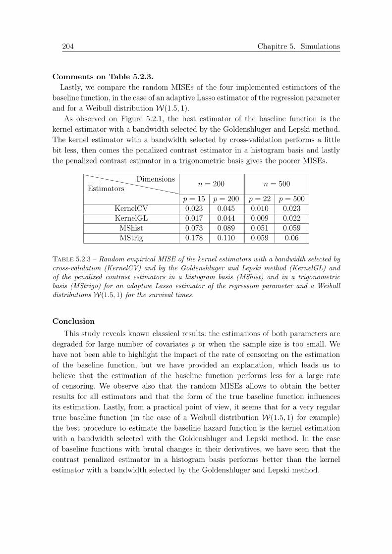
204 Chapitre 5. Simulations
Comments on Table 5.2.3.
Lastly, we compare the random MISEs of the four implemented estimators of thebaseline function, in the case of an adaptive Lasso estimator of the regression parameterand for a Weibull distribution W(1.5, 1).
As observed on Figure 5.2.1, the best estimator of the baseline function is thekernel estimator with a bandwidth selected by the Goldenshluger and Lepski method.The kernel estimator with a bandwidth selected by cross-validation performs a littlebit less, then comes the penalized contrast estimator in a histogram basis and lastlythe penalized contrast estimator in a trigonometric basis gives the poorer MISEs.
❵❵❵❵❵❵❵
❵❵
❵❵
❵❵❵❵
EstimatorsDimensions
n = 200 n = 500
p = 15 p = 200 p = 22 p = 500KernelCV 0.023 0.045 0.010 0.023KernelGL 0.017 0.044 0.009 0.022MShist 0.073 0.089 0.051 0.059MStrig 0.178 0.110 0.059 0.06
Table 5.2.3 – Random empirical MISE of the kernel estimators with a bandwidth selected bycross-validation (KernelCV) and by the Goldenshluger and Lepski method (KernelGL) andof the penalized contrast estimators in a histogram basis (MShist) and in a trigonometricbasis (MStrigo) for an adaptive Lasso estimator of the regression parameter and a Weibulldistributions W(1.5, 1) for the survival times.
Conclusion
This study reveals known classical results: the estimations of both parameters aredegraded for large number of covariates p or when the sample size is too small. Wehave not been able to highlight the impact of the rate of censoring on the estimationof the baseline function, but we have provided an explanation, which leads us tobelieve that the estimation of the baseline function performs less for a large rateof censoring. We observe also that the random MISEs allows to obtain the betterresults for all estimators and that the form of the true baseline function influencesits estimation. Lastly, from a practical point of view, it seems that for a very regulartrue baseline function (in the case of a Weibull distribution W(1.5, 1) for example)the best procedure to estimate the baseline hazard function is the kernel estimationwith a bandwidth selected with the Goldenshluger and Lepski method. In the caseof baseline functions with brutal changes in their derivatives, we have seen that thecontrast penalized estimator in a histogram basis performs better than the kernelestimator with a bandwidth selected by the Goldenshluger and Lepski method.

5.6. Application to a real dataset on breast cancer 205
5.6 Application to a real dataset on breast cancer
In this section, we apply the proposed method to study the relapse free survival(RFS) from breast cancer adjusted on high-dimensional covariates in two groups ofpatients. We consider a Cox model (2.105) to link the RFS to the covariates. We aimat answering the two questions of the introduction concerning the biomarkers thatinfluence the RFS and the prediction of the RFS for each individual. The dataset isavailable on the website www.ncbi.nlm.nih.gov/geo/query/acc.cgi?acc=GSE6532.
The dataset consists of 414 patients in the cohort GSE6532 collected by Loi et al.(2007) for the purpose of characterizing Estrogen Receptor (ER)-positive subtypeswith gene expression profiles. Estrogen receptors are a group of proteins found insidecells, which is activate by the hormone estrogen. There are different forms of theestrogen receptors, referred to as subtypes of estrogen receptors. When they are overexpressed, they are referred to as ER-positive. The dataset has been studied froma survival analysis point of view in Tian et al. (2012). Following them, we applyour procedures to the same survival time of interest (the RFS). Excluding patientswith incomplete informations, as it is done by Loi et al. (2007), there are 142 patientsreceiving Tamoxifen and 104 untreated patients. It should be underlined that we shoulddo better to handle the missing data, but in this study we also exclude the patientswith missing data. In addition to clinical informations such as the age or the size ofthe tumor (the complete clinical informations are listed in Table (C.0.1) in AppendixC), we have 44 928 gene expression measurements for each of the 246 patients. Twodifferent survival times are available in this study: the time of relapse free survival andthe time of distant metastasis free survival. We are interested in this study in the timeof relapse free survival, which subjects to right censoring due to incomplete follow-up.There are 60% of censorship in the group of the untreated patients and 66% in thegroup of patients receiving Tamoxifen. Our goal is to compare the baseline functionsin the two groups of patients: the patients receiving Tamoxifen and the untreatedpatients.
We start by a preliminary variable selection among the 44928 levels of gene expres-sion. This corresponds to a screening step (see Fan et al. (2010)). This preliminaryvariable selection is based on the score statistics of each Cox model considered for eachvariable separately. We only keep the variables which score statistics are superior to athreshold. The difference from the procedure proposed by Fan et al. (2010) is that wefix the number of covariates we want to keep and then we tune a threshold to selectthis number of covariates. We define four different thresholds. The first one is definedas the 95th percentile of a Chi-squared distribution with 1 degree of freedom, so that996 probesets have been selected and with the clinical covariates we have p = 1000. We

206 Chapitre 5. Simulations
then take 3 other thresholds such that we can work alternatively with p = 6, p = 10
and p = 100 covariates.We refer to Appendix C for a detailed description of the data contained in R
workspace.
5.6.1 Variable selection
Comments on Table 6.1.1.
Table 6.1.1 recapitulates the variables that have been selected by the one step Lasso,the one step Lasso associated to a maximum Cox partial log-likelihood procedure andthe adaptive Lasso associated to a maximum Cox partial log-likelihood procedureprocedure for different values of p in the two groups of patients.
❵❵❵❵❵
❵❵
❵❵❵❵❵❵❵❵
Group of patientsp
p = 6 p = 10 p = 100 p = 1000
Untreated size size size+2 g.e. size+15 g.e.size+3g.e. adap: size+18 g.e.
Tamoxifen grade grade 10 g.e. 24 g.e.adap: 9 g.e. adap: 38 g.e.
Table 6.1.1 – Selected variables in the two groups of patients. We precise the name of theclinical selected variables and only give the number of selected genes (e.g.=gene expression).
In the group of untreated patients, the covariate "size", which corresponds to thetumor size in centimeter, is the only clinical variable selected for all considered p.When p >
√n the procedures select also some genes that explain the time of relapse
free survival: 2 probesets when p = 100 and 15 probesets when p=1000 (18, for theadaptive Lasso procedure).
Concerning the patients receiving Tamoxifen, when p ≤ √n, the clinical variable
"grade", which corresponds to histologic grade (Elston-Ellis) category, is the onlyvariable that seems explain the time of relapse free survival and when p > n someprobesets are also selected.
We have considered two different models for each treatment group, we now inves-tigate if one model could be fitted for all the cohort with the treatment as a covariate.
5.6.2 Estimation of the baseline hazard function
Comments on Figures 6.2.1 and 6.2.2.
Figures 6.2.1 and 6.2.2 show the graphs of the estimators of the baseline functionvia the kernel estimator with a bandwidth selected by cross-validation, the kernelestimator with a bandwidth select with the Goldenshluger and Lepski method and thepenalized contrast estimator in histogram and trigonometric bases respectively, in thetwo groups of patients for p = 10, 100, 1000.

5.6. Application to a real dataset on breast cancer 207
0 2 4 6 8 10 12
0.02
0.03
0.04
0.05
0.06
0.07
0.08
0.09
temps_untreat
estimators_untreat
alpha_histalpha_noyalpha_GL
(a) Untreated patients (p=10).
0 2 4 6 8 10
0.00
0.02
0.04
0.06
0.08
0.10
temps_tamox
estimators_tamox
alpha_trig
alpha_noy
alpha_GL
(b) Tamoxifen patients (p=10).
0 2 4 6 8 10 12
0.02
0.03
0.04
0.05
0.06
0.07
0.08
0.09
temps_untreat
estimators_untreat
alpha_histalpha_noyalpha_GL
(c) Untreated patients (p=100).
0 2 4 6 8 10
0.00
0.02
0.04
0.06
0.08
0.10
temps_tamox
estimators_tamox
alpha_trigalpha_noyalpha_GL
(d) Tamoxifen patients (p=100).
0 2 4 6 8 10 12
0.05
0.10
0.15
0.20
0.25
temps_untreat
estimators_untreat
alpha_hist
alpha_noy
alpha_GL
(e) Untreated patients (p=1000).
0 2 4 6 8 10
0.00
0.02
0.04
0.06
0.08
0.10
temps_tamox
estimators_tamox
alpha_trig
alpha_noy
alpha_GL
(f) Tamoxifen patients (p=1000).
Figure 6.2.1 – Kernel estimators with a bandwidth selected either by cross-validation (ingreen) or by the Goldenshluger and Lepski method (in black) and by model selection estimatorin the histogram basis (in blue). The first column is associated to the group of untreatedpatients and the second column corresponds to the group of Tamoxifen patients for p = 10(first line), p = 100 (second line) and p = 1000 (third line).

208 Chapitre 5. Simulations
0 2 4 6 8 10 12
0.02
0.03
0.04
0.05
0.06
0.07
0.08
0.09
temps_untreat
estimators_untreat
alpha_trigalpha_noyalpha_GL
(a) Untreated patients (p=10).
0 2 4 6 8 10
0.00
0.02
0.04
0.06
0.08
0.10
temps_tamox
estimators_tamox
alpha_trig
alpha_noy
alpha_GL
(b) Tamoxifen patients (p=10).
0 2 4 6 8 10 12
0.02
0.03
0.04
0.05
0.06
0.07
0.08
0.09
temps_untreat
estimators_untreat
alpha_trig
alpha_noy
alpha_GL
(c) Untreated patients (p=100).
0 2 4 6 8 10
0.00
0.02
0.04
0.06
0.08
0.10
temps_tamox
estimators_tamox
alpha_trig
alpha_noy
alpha_GL
(d) Tamoxifen patients (p=100).
0 2 4 6 8 10 12
0.02
0.03
0.04
0.05
0.06
0.07
0.08
0.09
temps_untreat
estimators_untreat
alpha_trig
alpha_noy
alpha_GL
(e) Untreated patients (p=1000).
0 2 4 6 8 10
0.00
0.02
0.04
0.06
0.08
0.10
temps_tamox
estimators_tamox
alpha_trig
alpha_noy
alpha_GL
(f) Tamoxifen patients (p=1000).
Figure 6.2.2 – Kernel estimator with a bandwidth selected either by cross-validation (ingreen) or by the Goldenshluger and Lepski method (in black) and model selection estimatorin the trigonometric basis (in blue). The first column is associated to the group of untreatedpatients and the second column corresponds to the group of Tamoxifen patients for p = 10(first line), p = 100 (second line) and p = 1000 (third line).

5.6. Application to a real dataset on breast cancer 209
A first remark is that on Figures 6.2.1d and 6.2.1f, the plots of the kernel esti-mators with a bandwidth selected either by cross-validation or by the Goldenshlugerand Lepski method are overlaid. This means that the two estimators give the sameestimations of the baseline hazard ratio. Then, we observe that the more the time goesby, the more the baseline function is high for the untreated patient compared withthose receiving tamoxifen. Indeed at time 10 the estimators of the baseline functionfor the untreated patients are exploding whereas those of the Tamoxifen patient arebounded and tend to decrease. This leads us to believe that the treatment has a posi-tive influence on the survival time. Then, for p = 10 and p = 100, the baseline functionin the two groups of patients are not proportional and thus, we can not consider aCox model with a mix of the two groups of patients. But, for p = 1000, it seemsthat the baseline hazard functions are proportional. In this case, we could thereforeconsider a Cox model by grouping all the patients and adding the treatment to themodel as a covariate to study the effect of the treatment on the survival time. As thesets of selected variables in the two groups of patients are different (in particular theselected probesets are not the same), a more interesting work would be to consider aninteraction model to investigate potential crossed effects of the treatment and somegenes.

210 Chapitre 5. Simulations
Appendix
A The rectangle method
The rectangle method computes an approximation of a definite integral of a func-tion f , made by covering the area under the graph of f with a collection of rectangleswhose heights are determined by the values of the function. Specifically, the interval(a, b) over which the function f is to be integrated is divided into N equal subintervalsof length h = (b − a)/N . The rectangles are then drawn so that either their left orright corners, or the middle of their top line lies on the graph of the function, withbases running along the x-axis. The approximation to the integral is then calculatedby adding up the areas of the N rectangles, giving the formula:
∫ b
a
f(x)dx ≈ h
N∑
n=1
f(xn)
where h = (b− a)/N and xn = a+ nh.The formula for xn above gives xn for the top-right corner approximation.As N gets larger, this approximation gets more accurate. In fact, this computation
is the spirit of the definition of the Riemann integral and the limit of this approximationas n → ∞ is defined and equal to the integral of f on (a,b) if this Riemann integralis defined. Note that this is true regardless of which top line is used, however themidpoint approximation tends to be more accurate for finite n.
B Calibration of the constants
B.1 In model selection
The penalty term in model selection is defined by (5.14), where κ is a universalconstant. To determine this constant, we consider a grid of constants κ = (κ1, ..., κK).For k = 1, ..., K, we determine mβ(κk) = argmin
mCn(α
βm, β) + pen(m,κk), where
pen(m,κk) = κk(1 + ||αβ
max(m)||∞,τ )Dm
n, for k = 1, ..., K,
and we obtain K estimators (αβ
mβ(κk))k=1,...,K . Then, we compute, for each estimator,
the random Integrated Squared Error (ISErand) defined and approximated via the

B. Calibration of the constants 211
rectangle method by
ISErand(κk) =1
n
n∑
i=1
∫ τ
0
(αβ
mβ(κk)(t)− α0(t))
)2eβ
TZiYi(t)dt, for k = 1, .., K.
≈ 1
n
n∑
i=1
eβTZi
N∑
j=1
(αβ
mβ(κk)(uj)− α0(uj)
)21Xi≥uj
τ
N,
where N = 100, and (uj)j are grid points evenly distributed across [0, τ ]. Lastly, weconduct a new Monte Carlo study with Ne = 500 replications and approximate theempirical random Mean Integrated Squared Errors (MISErand) for each κ in the grid:for k = 1, ..., K,
MISErandemp(κk) =1
Ne
Ne∑
j=1
(ISErand(κk))j. (5.22)
We finally choose the constant κ that minimizes the empirical MISErandemp (5.22).Since the constant κ is universal, we should obtain the same κ for different dis-tributions of the survival time. In order to observe this, we iterate all the proce-dure for three Weibull distributions with different parameters (W(0.5, 1), W(1, 1) andW(3, 1)). We consider the grid κ = (0.1, 0.5, 1, 2, 5, 8, 10) in the case of histograms andκ = (0.1, 0.5, 1, 2, 5, 8, 10, 15, 20) in the trigonometric case.
0 2 4 6 8 10
0.213
0.216
0.219
grille_kappa
R_hist_1$x
W(0.5,1)
0 2 4 6 8 10
0.00
0.04
0.08
0.12
grille_kappa
R_hist_2$x
W(1,1)
0 2 4 6 8 10
0.06
0.10
0.14
0.18
grille_kappa
R_hist_3$x
W(3,1)
Figure B.1.1 – Plots of the empirical random MISEs of αβ
mβ(κk)as functions of κ in the
case of histograms.
Figures B.1.1 represents graphically the empirical random MISEs of αβ
mβ(κk)as
functions of κ in the case of histograms (we proceed similarly in the case of a trigono-metric basis). On Figure B.1.1, we observe clearly the U-form in the cases of W(0.5, 1)

212 Chapitre 5. Simulations
and W(3, 1) distributions, it is less visible for the W(1, 1) distribution. In this case, wecould have considered a largest grid Hn with greatest values, but from the constraintof the two other cases, we choose for the three distributions the fifth value, whichseems to be the more suitable intersection. This corresponds to the choice of κ = 5.
B.2 In Goldenshluger and Lepski method
The variance term V (h) in the Goldenshluger and Lepski method is defined by(5.18), where κ′ is a universal constant. The principle to determine this constant isclose to the one in model selection to determine the universal constant in the penaltyterm, so that we explain the procedure more briefly in this case.
We consider a grid of constants κ′ = (10−4, 0.1, 1, 10, 1000). We calculate for eachconstant κ′
k, k = 1, ..., K ′,
hβ(κ′k) = argmin
h∈Mn
Aβ(h) + V β(h, κ′k), where V β(h, κ′
k) = κ′k
||αβ
max(h)||∞,τ ||K||22nh
.
Then, we compute the random Integrated Squared Error (ISErand) defined for k =
1, ..., K ′ by
ISErand(κ′k) =
1
n
n∑
i=1
∫ τ
0
(αβ
hβ(κ′k)(t)− α0(t)
)2eβ
TZiYi(t)d(t)
≈ 1
n
n∑
i=1
eβTZi
N∑
j=1
(αβ
hβ(κ′k)(uj)− α0(uj)
)21Xi≥uj
τ
N,
where N = 100, and (uj)j are grid points evenly distributed across [0, τ ] and theapproximation comes from the rectangle method (see Appendix A). Lastly, we conducta new Monte Carlo study with Ne = 500 replications: for k = 1, ..., K ′,
MISErandemp(κ′k) =
1
Ne
Ne∑
j=1
(MISErand(κ′k))j. (5.23)
We finally choose the constant κ′ that minimizes (5.23) for three Weibull distributionswith different parameters (W(0.5, 1), W(1, 1) and W(2, 1)). This study leads to chooseκ′ = 1.
C Description of the real data
Demographics file containing the clinical information for the untreated
patients (137) and the tamoxifen treated patients (277).
The clinical information are listed in Table (C.0.1).

C. Description of the real data 213
Notations Definitionssamplename unique id for the patient
id original id for the patients(id given by the institution,
useful to look for intersection between multiple datasets)series arbitrary name to specify the institutionage age in years
grade histologic grade (Elston-Ellis) categorysize tumor size in cmer estrogen receptor statuspgr progesterone receptor statusnode nodal statust.rfs time of relapse free survivale.rfs event of relaps free survival
t.dmfs time of distant metastasis free survivale.dmfs event of distant metastasis free survival
treatment type of treatment (none/tamoxifen)
Table C.0.1 – Table of the clinical information
R workspace containing the following objects:
data.untreated: matrix of gene expressions with the untreated patients in rows(137) and the affy probesets in columns (44928). The probesets are all the probsetsfrom the chip hgu133a and the chip hgu133b (with some probesets being renamedwith "_2" because of same name than in hgu133a chip). RMA normalization wasperformed separately for each population ("series" in demo) and all the probesetswere median centered.
demo.untreated: matrix with clinical information concerning the untreated pa-tients (137).
annot.untreated: annotations of all the probesets (44928).
data.tam: matrix of gene expressions with the tamoxifen treated patients in rows(277) and the affy probesets in columns (44928). The probesets are all the probsetsfrom the chip hgu133a and the chip hgu133b (with some probesets being renamedwith "_2" because of same name than in hgu133a chip). The chip hgu133plus2 wasused for "GUYT" series and only the common probesets with hgu133a/b were keptfor further analysis. RMA normalization was performed separately for each population("series" in demo) and all the probesets were median centered.

214 Chapitre 5. Simulations
demo.tam: matrix with clinical information concerning the tamoxifen treatedpatients (277).
annot.tam: annotations of all the probesets (44928).
Conclusion
Les travaux présentés dans cette thèse portent sur l’estimation de l’intensitéd’un processus de comptage dans un modèle à intensité multiplicative d’Aalen enprésence d’un grand nombre de covariables. Nous avons envisagé plusieurs approchespour différents modèles. Dans la Partie I, nous avons considéré l’intensité commefonction non-paramétrique du temps et des covariables et nous l’avons estimée parune fonction satisfaisant un modèle de Cox non-paramétrique. Nous avons proposéune procédure Lasso spécifique à la grande dimension pour estimer simultanémentles deux paramètres du modèle de Cox. Dans la Partie II, nous avons supposé quel’intensité vérifiait un modèle de Cox. Pour estimer les deux paramètres du modèle,nous avons alors opté pour des procédures en deux étapes, permettant d’estimerle paramètre de régression associé aux covariables à l’aide d’une procédure Lasso,spécifique à la grande dimension, et de proposer des procédures d’estimation du risquede base, fonction du temps, par des procédures usuellement utilisées en estimationnon-paramétrique, mais non spécifiques à la grande dimension. Nous avons établi desinégalités oracles non-asymptotiques pour l’estimateur de l’intensité complète (PartieI) et pour les estimateurs du risque de base obtenus par sélection de modèles et parl’estimation à noyaux avec un choix de fenêtre par la méthode de Goldenshluger etLepski (Partie II). Ces résultats sont les premiers résultats non-asymptotiques obtenusdans un cadre de grande dimension pour les covariables. Nous avons de plus montréque les procédures pour estimer le risque de base à la Partie II sont pertinentesen pratique et sont au moins aussi performantes que les procédures existantes. Cestravaux, considérés dans le cadre général des processus de comptage, ont été motivéspar la question pratique de la prédiction de la durée de survie d’un individu pour unemaladie donnée. En cela, les procédures proposées, ainsi que les résultats théoriques etpratiques permettent de répondre à cette question. Il reste tout de même différentespistes de recherche à envisager afin de poursuivre l’étude que nous avons menée et del’étendre à d’autres types de problèmes.
Perspectives de recherche
Dans les deux parties de cette thèse, nous avons établi des inégalités oracles pourles estimateurs obtenus. Les vitesses de convergence obtenues pour ces estimateursimpliquent la taille de l’échantillon, comme c’est classiquement le cas, mais aussi un
216 Conclusion
terme de l’ordre du logarithme du nombre de covariables, spécifique au cadre de lagrande dimension étudié. Nous ne pouvons pour l’instant nous permettre d’affirmerl’optimalité de cette vitesse au sens minimax. Une perspective immédiate consistedonc à étudier la borne inférieure pour le risque minimax associé sur des boulesd’espaces de Besov.
Dans la Partie I, nous avons considéré le critère de la vraisemblance empiriquetotale de manière à estimer simultanément les deux paramètres du modèle de Coxnon-paramétrique. Ce critère n’est pas le critère usuellement considéré dans le modèlede Cox, puisque la procédure habituelle consiste d’abord à estimer le paramètre derégression à l’aide de la vraisemblance partielle de Cox et ensuite à considérer unestimateur à noyau du risque de base. À notre connaissance, les algorithmes existants àce jour pour estimer le paramètre de régression du modèle de Cox en grande dimension,tels que les algorithmes glmnet ou penalized dans R, sont programmés à partir de lavraisemblance partielle de Cox. Cependant, pour une fonction
λβ,γ(t,Zi) = exp( N∑
k=1
γkθk(t) +Ziβ)
(5.24)
avec les notations de la Partie I, la log-vraisemblance empirique définie par
Cn(λβ,γ) = − 1
n
n∑
i=1
∫ τ
0
log(λβ,γ(t,Zi))dNi(t)−∫ τ
0
λβ,γ(t,Zi)Yi(t)dt
,
est de la forme de celle associée à la régression poissonnienne. En effet, si ν1, ..., νnsont n variables aléatoires de loi de Poisson de paramètre λ, alors la log-vraisemblanceassociée à cet échantillon est définie par
− 1
nlogL(λ) = − 1
n
n∑
i=1
(νi log λ− λ).
Or la régression poissonnienne est implémentée dans les packages glmnet (pour dessauts positifs) et penalized de R. On pourrait donc utiliser ces algorithmes basés surune descente de coordonnées cycliques pour implémenter la procédure d’estimationde la Partie I. L’algorithme SPAMS implémenté sous MATLAB est un algorithme detype FISTA permettant aussi de considérer une procédure Lasso pour une régressionpoissonnienne. Cependant, le gradient de la vraisemblance n’étant pas Lipschitz, on neconnaît pas de résultat théorique garantissant la convergence de ces trois algorithmes.Cela donne néanmoins une possibilité de mise en pratique de notre procédure etdans un futur proche, nous nous attacherons à l’implémenter à l’aide d’un de cesalgorithmes. Cela permettra d’une part de vérifier les performances pratiques del’estimateur Lasso de l’intensité que nous proposons, et d’autre part d’introduire lespoids que nous obtenons et de comparer les procédures avec et sans les poids. De plus,
Conclusion 217
une fois la procédure de la Partie I implémentée, nous pourrons effectuer une étudecomparative des procédures proposées dans les Parties I et II de cette thèse.
Ensuite, une perspective naturelle, sera de s’intéresser à une des généralisationsclassique et très utilisée en pratique qui consiste à considérer des covariables et uncoefficient de régression qui dépendent du temps. Ainsi, nous avons par exemple ré-cemment amorcé un travail, en collaboration avec Mokhtar Alaya et Agathe Guilloux,dans lequel nous considérons un modèle de Cox avec un paramètre de régression quidépend du temps : pour tout t ≥ 0,
λ0(t,Z) = α0(t) exp(β0(t)TZ),
où Z = (Z1, ..., Zp)T est un vecteur de covariables p-dimensionnel et
β0(t) = (β01(t), ..., β0p(t))T est un vecteur de fonctions du temps p-dimensionnel.
L’idée est alors d’approximer chaque coordonnée du paramètre de régression β0(t)
par des histogrammes. Plus précisément, nous considérons des fonctions candidatesde la forme de (5.24), en supposant que les fonctions θk sont des histogrammes, i.e.θk = 1Ik pour k = 1, ..., N , où Ik est un intervalle, et en approximant β0(t) par unecombinaison linéaire de ces mêmes histogrammes. Nous obtenons donc des fonctionscandidates de la forme
λβ,γ(t,Z) = exp
(N∑
k=1
γk1Ik(t) +
p∑
j=1
N∑
k=1
βj,k1Ik(t)Zj
).
Nous étudierons alors les aspects algorithmiques et théoriques des procédures quiestiment des histogrammes pénalisés par leurs variations totales.
Dans la partie II, nous avons mené une étude sur une base de données sur le cancerdu sein. Nous avons ainsi montré que pour 1000 covariables les courbes du risque debase semblent avoir la même forme dans les deux groupes de patients considérés. Lemodèle de Cox étant un modèle à risque proportionnel, si les risques de base estimésdans les deux groupes de patients ont la même forme, nous pouvons regrouper lesindividus et considérer un nouveau modèle de Cox en ajoutant la variable traitement.De plus, les ensembles des variables sélectionnées dans les deux groupes de patientssont différents. Il se peut donc que certaines variables sélectionnées aient un effet enintéraction avec le traitement. Il serait donc intéressant dans notre étude d’étudier unmodèle de Cox en considérant la variable traitement comme une variable explicative eten ajoutant des termes d’interaction pour mettre en évidence l’effet combiné du traite-ment et de certaines variables, lesquelles sont alors appelées chimio-sensibilisantes. Cetype d’étude mettant en évidence la relation d’interaction entre des facteurs génétiqueset le traitement fait partie des grandes questions statistiques en analyse de survie pour

218 Conclusion
la médecine personnalisée (voir Collura et al. (2014) pour un exemple de mise en évi-dence d’une interaction entre une anomalie au niveau du génome et le traitement).De plus, des travaux récents portent sur le Lasso dans des modèles à interaction (voirBien et al. (2013) par exemple). Il serait donc intéressant d’approfondir notre étudeen considérant ces modèles.

A
Appendices
SommaireA.1 Un peu de théorie sur les processus de comptage . . . . . . . . . . . 220
A.2 Construction de la vraisemblance de Cox . . . . . . . . . . . . . . . 224
A.3 Quelques inégalités de concentration . . . . . . . . . . . . . . . . . . 227
A.3.1 Inégalité de Bernstein standard . . . . . . . . . . . . . . . . . . . . . 227
A.3.2 Inégalité de Bernstein pour les martingales . . . . . . . . . . . . . . . 227
A.3.3 Inégalité de Talagrand . . . . . . . . . . . . . . . . . . . . . . . . . . 227
219
220 A. Appendices
A.1 Un peu de théorie sur les processus de comp-
tage 1 :
Processus stochastiques et notions de base
Tous les phénomènes étudiés dans ce travail se déroulent en temps continu. Fixons,pour la suite, un intervalle T = [0, τ [ de R+ qui indexera le temps. Soient (Ω,F ,P)
un espace probabilisé, où F une σ-algèbre et P une mesure de probabilité définie surF . On appelle filtration une famille (Ft)t∈T croissante et continue à droite (càd) desous-tribus, c’est-à-dire telle que :
(i) Fs ⊆ Ft pour tout s ≤ t dans T (croissante)
(ii) Fs =⋂
t>s Ft pour tout s ∈ T (càd).
Un processus stochastique W est alors une famille de variables aléatoires (v.a.)W (t), t ∈ T indexées par le temps. On dira que W est adapté à la filtration (Ft)t∈Tsi pour tout t dans T , la v.a. W (t) est Ft-mesurable. Pour un ω dans Ω, on appelleratrajectoire de W la fonction t 7→ W (t, ω). Le processus W est alors dit càdlàg siP-presque toutes ses trajectoires appartiennent à l’espace D(T ) des fonctions càdlàg(continues à droite, limites à gauche) sur T , appelé espace de Skorohod dans la théoriede la convergence faible (voir Billingsley (1968)). Il est dit prévisible si, en tant quefonction de (t, ω) ∈ T ×Ω, il est mesurable par rapport à la tribu sur T ×Ω engendréepar les processus càg et adaptés.
À tout processus W càdlàg, on peut, grâce au résultat de Courrège & Priouret(1965), associer une filtration « historique » (Ft)t∈T telle que, pour tout t dans T , lasous-tribu Ft = σW (s), s ≤ t ∈ T est engendrée par le passé à t du processus. Cettefamille peut être complétée en ajoutant les négligeables à la tribu F0 sans qu’elle perdesa propriété de filtration. Par construction, le processus W est adapté à (Ft)t∈T .
On appellera temps d’arrêt une v.a. T à valeurs dans T = [0, τ ] telle que lesévénements T ≤ t sont Ft-mesurables pour tout t dans T . Une suite localisante detemps d’arrêt est une suite (Tn) croissante de temps d’arrêt telle que :
P(Tn > t) →n→∞
1,
pour tout t dans T . On dira qu’un processus vérifie localement une propriété s’il existeune suite localisante (Tn) telle que le processus I(Tn > 0)XT la vérifie, où XT estle processus arrêté à T tel que
XT (.) = X(. ∧ T ).
Martingales à temps continu :
Une martingale M par rapport à la filtration (Ft) est un processus stochastiquecontinu à droite avec limite à gauche tel que :
1. Nous nous sommes inspirés de la thèse de Guilloux (2004) pour écrire cette annexe

A.1. Un peu de théorie sur les processus de comptage 221
(i) M est Ft-adapté
(ii) E|M(t)| < ∞ for all s ≤ t,
(iii) E(M(t)|Fs) = M(s) for all s ≤ t
Une martingale M est dite de carré intégrable si :
supt∈T
E(M(t)2
)< ∞.
Un processus M est une martingale locale s’il existe une suite localisante (Tn) de tempsd’arrêt telle que, pour tout n, le processus I(Tn > 0)MTn soit une martingale. Unemartingale locale est un processus càdlàg et adapté. Si, de plus, la suite (Tn) peut êtrechoisie de telle sorte que I(Tn > 0)MTn soit de carré intégrable, alors M est unemartingale locale de carré intégrable.
Nous donnons maintenant une version du célèbre Théorème de décomposition deDoob-Meyer.
Définition A.1 (Décomposition de Doob-Meyer). Pour un processus W càdlàg et
adapté, on définit, s’il existe, son compensateur comme l’unique processus W prévi-
sible, càdlàg, à variation finie et tel que le processus W −W soit une martingale locale
nulle en zéro.
En particulier, si M est une martingale locale de carré intégrable, il existe ununique processus prévisible, càdlàg, à variation finie et nul en zéro, noté 〈M,M〉 ou〈M〉, tel que M2 − 〈M,M〉 soit une martingale locale. On appelle 〈M〉 la variation
prévisible de M . Si la variation prévisible est une fonction déterministe, on parlera alorsde fonction de variance de M . On introduit aussi le processus de variation optionnel
de M , noté [M,M ] ou [M ] et défini pour t ∈ T , par [M ]t =∑
s≤t(∆M(s))2, avec∆M = M(t)−M(t−).
Théorème A.1. Soient M une martingale locale de carré intégrable et à variation
finie et H un processus prévisible localement borné. L’intégrale stochastique∫HdM
définie pour tout t dans T et presque tout w dans Ω par :
∫ t
0
H(w, s)dM(w, s)
est alors une martingale locale de carré intégrable et à variation finie. On a de plus :
⟨∫HdM
⟩=
∫H2d〈M〉 and
[ ∫HdM
]=
∫H2d[M ].
Processus de comptage :
En notant (Ω,F ,P) l’espace probabilisé filtré par F = (Ft)t∈T sur lequel on tra-vaille, on dira que N = (N1, ..., Nn) est un processus de comptage s’il est adapté et telque :

222 A. Appendices
(i) les applications t 7→ Ni(t), pour i = 1, ..., n, sont càd, étagées, nulles en zéro etadmettent un nombre dénombrable de sauts de longueur +1;
(ii) deux processus Ni et Nj, pour i 6= j, ne peuvent sauter en même temps.
On suppose de plus que, pour tout i = 1, ..., n, la v.a. Ni(t) est p.s. finie pour toutt positif. Pour le processus N , les instants de saut Tk = inft :
∑ni=1 Ni(t) ≥ k
sont des (Ft)-temps d’arrêt. On pose Tk = τ si k >∑n
i=1 Ni(τ). Les composantes Ni,pour i = 1, ..., n, sont des processus adaptés, càdlàg, croissants et localement bornés(0 ≤ NTk
i (t) ≤ n). Ils admettent des compensateurs notés Λi croissants tels que, pourtout i = 1, ..., n, le processus :
Mi = Ni − Λi
soit une martingale locale de carré intégrable dont le processus de variation prévisibleest donné par 〈Mi〉 = Λi −
∫∆ΛidΛi. De plus, on a 〈Mi,Mi′〉 = −
∫∆ΛidΛi′ pour
i 6= i′. On a pour tout t ∈ T et i = 1, ..., n, E[Ni(t)] = E[Λi(t)]. De plus, dans le cascontinu, il existe, pour i = 1, ..., n, des processus prévisibles fi, appelés intensités, telsque
Λi(t) =
∫ t
0
fi(s)ds.
On dit que les processus Ni sont des processus de comptage à intensité.Par définition, le processus de variation optionnel de Mi = Ni − Λi est défini par
[Mi] = Ni et par unicité du compensateur, le processus de variation prévisible estdéfini par 〈Mi〉 = Λi.
Cas général : les processus de comptage marqué
Les processus de comptage marqués sont une généralisation des processus de comp-tage. L’idée est la suivante : au lieu de ne considérer que les instants Tk auquel se pro-duit un évènement spécifique comme c’est le cas pour les processus de comptage, nousobservons aussi une variable supplémentaire Zk à chaque instant Tk. Plus précisément,fixons un espace mesurable (E, E) appelé espace marqué, et supposont que
(i) (Zk, k ≥ 1) est une suite de variables aléatoires dans E,
(ii) la suite (Tk, k ≥ 1) constitue un processus de comptage
N(t) =∑
k
1Tk≤t.
La suite de couple (Tk, Zk) est appelée processus ponctuel marqué, où les Zk sont lesmarques. Pour tout A ∈ E , nous pouvons définir le processus de comptage
Nt(A) =∑
k
1Tk≤t1Zk∈A,
qui compte le nombre de sauts avant t dont les marques sont dans A.
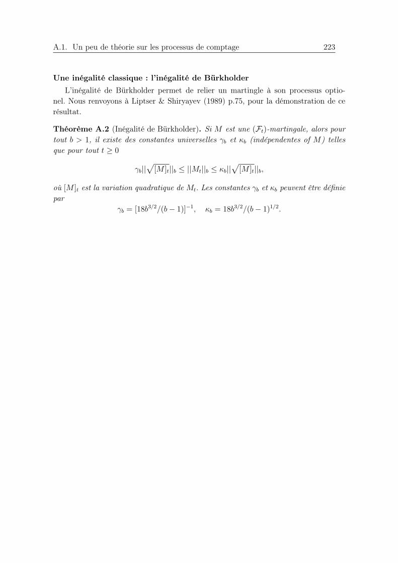
A.1. Un peu de théorie sur les processus de comptage 223
Une inégalité classique : l’inégalité de Bürkholder
L’inégalité de Bürkholder permet de relier un martingle à son processus optio-nel. Nous renvoyons à Liptser & Shiryayev (1989) p.75, pour la démonstration de cerésultat.
Théorème A.2 (Inégalité de Bürkholder). Si M est une (Ft)-martingale, alors pour
tout b > 1, il existe des constantes universelles γb et κb (indépendentes of M) telles
que pour tout t ≥ 0
γb||√
[M ]t||b ≤ ||Mt||b ≤ κb||√
[M ]t||b,
où [M ]t est la variation quadratique de Mt. Les constantes γb et κb peuvent être définie
par
γb = [18b3/2/(b− 1)]−1, κb = 18b3/2/(b− 1)1/2.

224 A. Appendices
A.2 Construction de la vraisemblance de Cox
Soient N1, ..., Nn des processus de comptage i.i.d., vérifiant le modèle à intensitémultiplicative d’Aalen (1.3) et pour i = 1, ..., n, la fonction de risque λ0(.,Zi) est définieselon le modèle de Cox (1.1). On observe On = (Zi, Ni(t), Yi(t), i = 1, ..., n, 0 ≤ t ≤ τ)
l’ensemble des observations. Pour tout i et tout t ∈ [0, τ ], d’après la décomposition deDoob-Meyer, nous avons
dNi(t) = α0(t)eβT0ZiYi(t)dt+ dMi(t),
où Mi est une martingale locale de carré intégrable. Pour i = 1, ..., n, comme les Ni,sont des processus de comptage indépendants, le processus agrégé N =
∑ni=1 Ni est
encore un processus de comptage qui vérifie
dN(t) = α0(t)1
n
n∑
i=1
eβT0ZiYi(t)dt+ dM(t),
avec M =∑n
i=1 Mi. Pour tout β ∈ Rp, notons
nSn(t,β) =n∑
i=1
eβT0ZiYi(t),
et définissons γ0(t) = α0(t)Sn(t,β0). Avec ces notations nous avons
dN(t) = γ0(t)dt+ dM(t).
D’après la formule de Jacod (voir Andersen et al. (1993)), la log-vraisemblance pour les
processus de comptage basée sur les observations O = (N(t), Y (t), 0 ≤ t ≤ τ) vérifie :
L(γ; O) =
∫ τ
0
log(γ(t))dN(t)−∫ τ
0
γ(t)dt (A.1)
L’estimateur du maximum de vraisemblance de γ0 est alors défini formellement par
γ = argmaxγ
∫ τ
0
log(γ(t))dN(t)−∫ τ
0
γ(t)dt
.
D’après (A.1), la log-vraisemblance pour estimer les deux paramètres du modèle deCox vérifie
L(α,β;On) =1
n
n∑
i=1
∫ τ
0
log(α(t)eβTZi)dNi(t)−
∫ τ
0
α(t)eβTZiYi(t)dt
,

A.2. Construction de la vraisemblance de Cox 225
que l’on peut décomposer en
L(α,β;On) =1
n
n∑
i=1
∫ τ
0
log
(α(t)Sn(t,β)
eβTZi
Sn(t,β)
)dNi(t)−
∫ τ
0
α(t)Sn(t,β)dt
=1
n
n∑
i=1
∫ τ
0
log
(eβ
TZi
Sn(t,β)
)dNi(t) (A.2)
+
∫ τ
0
log(α(t)Sn(t,β))dN(t)−∫ τ
0
α(t)Sn(t,β)dt. (A.3)
Le terme (A.3) correspond à la vraisemblance (A.1) pour γ(t) = α(t)Sn(t,β). Ondéfinit alors le terme (A.2) comme la vraisemblance partielle de Cox :
l∗n(β) =1
n
n∑
i=1
∫ τ
0
log
(eβ
TZi
Sn(t,β)
)dNi(t)
=1
n
n∑
i=1
∫ τ
0
log
(eβ
TZi
Sn(t,β)
)α0(t)e
βT0ZiYi(t)dt+
1
n
n∑
i=1
∫ τ
0
log
(eβ
TZi
Sn(t,β)
)dMi(t).
où le deuxième terme est centré.Nous pouvons construire un estimateur de type Breslow. Toujours, d’après la dé-
composition de Doob-Meyer, nous avons
1
n
n∑
i=1
∫ τ
0
dNi(t)
Sn(t,β)=
1
n
n∑
i=1
∫ τ
0
α0(t)eβ
TZiYi(t)
Sn(t,β)dt+
1
n
n∑
i=1
∫ τ
0
dMi(t)
Sn(t,β).
Le deuxième terme de droite en dMi est centré peut être interprété comme un bruitaléatoire. En β0, on peut écrire l’approximation suivante
1
n
n∑
i=1
∫ τ
0
dNi(t)
Sn(t,β0)≈∫ τ
0
α0(t)dt,
on dit que 1n
∑ni=1 dNi(t)/Sn(t,β0) « estime » α0(t)dt. Dans le cas particulier de la
censure aléatoire à droite, cela revient à dire que 1nδi/Sn(Xi,β0) « estime » α0(Xi).
On retrouve une justification de l’estimateur de Breslow et de Ramlau-Hansen (1983b).Dans le cas de la censure aléatoire à droite, la vraisemblance partielle de Cox se
réécrit1
n
n∑
i=1
∫ τ
0
log
(eβ
TZi
Sn(t,β)
)dNi(t) =
1
n
n∑
i=1
δi log
(eβ
TZi
Sn(Xi,β)
),
avec (Xi, δi)i∈1,...,n i.i.d. Si on identifie eβTZi/Sn(t,β) à un estimateur de l’intensité
de Ni définie par eβT0Ziα0(t), on devrait donc avoir
1
n
n∑
i=1
∫ τ
0
log
(eβ
TZi
Sn(t,β)
)dNi(t)−
1
n
n∑
i=1
∫ τ
0
eβTZi
Sn(t,β)Yi(t)dt,

226 A. Appendices
où le deuxième terme est nul. On est bien en train d’estimer α0(t)eβT0Zi par maximum
de vraisemblance. En effet, la fonction de perte naturelle associée à la vraisemblancepartielle de Cox est définie par :
ℓ(β,β0) = −E
[1
n
n∑
i=1
∫ τ
0
log
(eβ
TZi
Sn(t,β)
)dNi(t)−
1
n
n∑
i=1
∫ τ
0
log
(eβ
T0Zi
Sn(t,β0)
)dNi(t)
]
qui se décompose par Doob-Meyer en
− 1
n
n∑
i=1
E
[∫ τ
0
log
(eβ
TZi
Sn(t,β)
Sn(t,β0
eβT0Zi
)α0(t)e
βT0ZiYi(t)dt
]
+1
n
n∑
i=1
E
[∫ τ
0
log
(eβ
TZi
Sn(t,β)
Sn(t,β0
eβT0Zi
)dMi(t)
]
où le deuxième terme est nul. La fonction de perte s’écrit donc
ℓ(β,β0) = − 1
n
n∑
i=1
E
[∫ τ
0
log
(eβ
TZi
Sn(t,β)
Sn(t,β0
eβT0Zi
)α0(t)e
βT0ZiYi(t)dt
].
On retrouve la fonction de perte en kullback introduite par Castellan et Letué (voirLetué (2000)).

A.3. Quelques inégalités de concentration 227
A.3 Quelques inégalités de concentration
A.3.1 Inégalité de Bernstein standard
Nous rappelons l’inégalité de Bernstein standard (voir Proposition 2.9 dans le livrede Massart (2007)).
Théorème A.3. Soient ζ1, ..., ζn, n variables aléatoires réelles indépendantes. Suppo-
sons qu’il existe des constantes positives v et c telles que pour tout entier m ≥ 2
n∑
i=1
E[|ζi|m] ≤ m!vcm−2. (A.4)
Pour tout réel positif x, nous avons
P(n∑
i
(ζi − E(ζi)) ≥ x) ≤ exp(− x2
2(v + cx).)
(A.5)
Lorsque les variables ζi sont bornées, |ζi| ≤ b pour tout i ∈ 1, ..., n, alors l’hypo-thèse (A.4) est satisfaite avec
v =n∑
i=1
E[ζ2i ] et c = b/3.
A.3.2 Inégalité de Bernstein pour les martingales
Rappelons l’inégalité de Bernstein pour les martingales (voir van de Geer (1995),Lemme 2.1).
Théorème A.4. Soit Mtt≥0 une martingale localement de carré intégrable par
rapport à la filtration Ftt≥0. Définissons le processus prévisible de Mt par
Vt = 〈M,M〉t, t ≥ 0, et ses sauts par ∆Mt = Mt −Mt−. Supposons que |∆Mt| ≤ K
pour tout t > 0 et un certain K tel que 0 ≤ K < ∞. Alors, pour tout a > 0, b > 0,
P(Mt ≥ a, Vt ≤ b2 pour un certain t) ≤ exp
[− a2
2(aK + b2)
].
A.3.3 Inégalité de Talagrand
L’inégalité de Talagrand est une inégalité de concentration qui permet de contrôlerle supremum d’un processus empirique sur une classe de fonctions. Plusieurs formesde cette inégalité existent. Nous donnons ici celle qui nous a servi dans cette thèse.On peut trouver une preuve de ce théorème chez Comte et al. (2008) (Lemme 6.1).
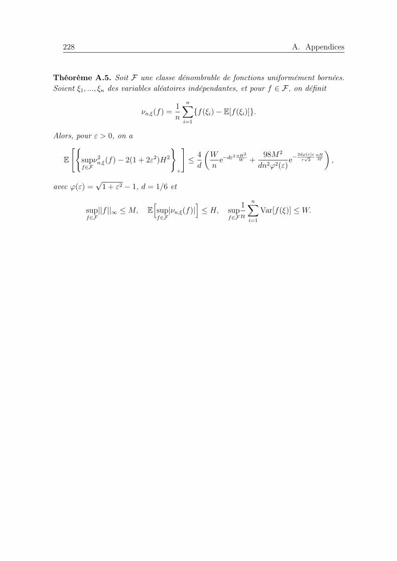
228 A. Appendices
Théorème A.5. Soit F une classe dénombrable de fonctions uniformément bornées.
Soient ξ1, ..., ξn des variables aléatoires indépendantes, et pour f ∈ F , on définit
νn,ξ(f) =1
n
n∑
i=1
f(ξi)− E[f(ξi)].
Alors, pour ε > 0, on a
E
[supf∈F
ν2n,ξ(f)− 2(1 + 2ε2)H2
+
]≤ 4
d
(W
ne−dε2 nH2
W +98M2
dn2ϕ2(ε)e− 2dϕ(ε)ε
τ√2
nHM
),
avec ϕ(ε) =√1 + ε2 − 1, d = 1/6 et
supf∈F
||f ||∞ ≤ M, E
[supf∈F
|νn,ξ(f)|]≤ H, sup
f∈F
1
n
n∑
i=1
Var[f(ξ)] ≤ W.

Bibliographie 229
Bibliographie
O. Aalen. A model for nonparametric regression analysis of counting processes. DansMathematical statistics and probability theory (Proc. Sixth Internat. Conf., Wisła,
1978), volume 2 de Lecture Notes in Statist., pages 1–25. Springer, New York, 1980.(Cité pages 5, 54 et 107.)
O.O Aalen. Statistical inference for a family of counting processes. PhD thesis, Uni-versity of California, Berkeley, 1975. (Cité page 7.)
O.O. Aalen. Nonparametric inference for a family of counting processes. The Annals
of Statistics, pages 701–726, 1978. (Cité page 7.)
H. Akaike. Information theory and an extension of the maximum likelihood prin-ciple. Dans In Second International Symposium on Information Theory (Tsahkad-
sor, 1971), pages 267–281. Akadémiai Kiadó, Budapest, 1973. (Cité pages 9, 18et 115.)
B. Altshuler. Theory for the measurement of competing risks in animal experiments.Mathematical Biosciences, 6:1–11, 1970. (Cité page 7.)
P. K. Andersen, Ø. Borgan, R. D. Gill, & Niels Keiding. Statistical models based on
counting processes. Springer Series in Statistics. Springer-Verlag, New York, 1993.ISBN 0-387-97872-0. (Cité pages 5, 29, 33, 54, 56, 93, 107, 109, 117, 153 et 224.)
P. K. Andersen & R. D. Gill. Cox’s regression model for counting processes: A largesample study. The Annals of Statistics, 10(4):pp. 1100–1120, 1982. ISSN 00905364.URL http://www.jstor.org/stable/2240714. (Cité pages 6, 7 et 184.)
A. Antoniadis, P. Fryzlewicz, & F. Letué. The Dantzig selector in Cox’s proportio-nal hazards model. Scandinavian Journal of Statistics, 37(4):pp. 531–552, 2010.ISSN 1467-9469. URL http://dx.doi.org/10.1111/j.1467-9469.2009.
00685.x. (Cité pages 29, 55 et 59.)
F. Bach. Self-concordant analysis for logistic regression. Electronic Journal of Statis-
tics, 4:pp. 384–414, 2010. (Cité pages 56, 61, 84 et 86.)
Y. Baraud. Model selection for regression on a fixed design. Probability Theory and
Related Fields, 117(4):467–493, 2000. (Cité page 18.)

230 Bibliographie
Y. Baraud. Model selection for regression on a random design. ESAIM: Probability
and Statistics, 6:127–146, 2002. (Cité pages 18 et 22.)
Y. Baraud. A Bernstein-type inequality for suprema of random processes with appli-cations to model selection in non-Gaussian regression. Bernoulli, 16(4):1064–1085,2010. (Cité page 128.)
A. Barron, L. Birgé, & P. Massart. Risk bounds for model selection via penalization.Probability theory and related fields, 113(3):301–413, 1999. (Cité pages 18, 22, 115et 121.)
P. L. Bartlett, S. Mendelson, & J. Neeman. l1-regularized linear regression: persistenceand oracle inequalities. Probability theory and related fields, 154(1-2):193–224, 2012.(Cité page 54.)
K. Bertin, C. Lacour, & V. Rivoirard. Adaptive estimation of conditional densityfunction. arXiv preprint arXiv:1312.7402, 2013. (Cité pages 26 et 27.)
K. Bertin, E. Le Pennec, & V. Rivoirard. Adaptive Dantzig density estimation. Annales
de l’IHP, Probabilités et Statistiques, 47(1):pp. 43–74, 2011. (Cité pages 11, 39, 61et 66.)
P. J. Bickel, B. Li, A. B. Tsybakov, S. A. van de Geer, B. Yu, T. Valdés, C. Rivero,J. Fan, & A. van der Vaart. Regularization in statistics. Test, 15(2):271–344, 2006.(Cité page 9.)
P. J. Bickel, Y. Ritov, & A. B. Tsybakov. Simultaneous analysis of Lasso and Dantzigselector. The Annals of Statistics, 37(4):pp. 1705–1732, 2009. ISSN 0090-5364. URLhttp://dx.doi.org/10.1214/08-AOS620. (Cité pages 11, 14, 15, 17, 18, 29,54, 55, 56, 59, 61, 62, 97, 98, 99, 100 et 102.)
J. Bien, J. Taylor, & R. Tibshirani. A lasso for hierarchical interactions. The Annals
of Statistics, 41(3):1111–1141, 2013. (Cité page 218.)
P. Billingsley. Convergence of probability measures. John Wiley, New York, 228:229,1968. (Cité page 220.)
L. Birgé. Model selection for density estimation with l2-loss. arXiv preprint
arXiv:0808.1416, 2008. (Cité page 18.)
L. Birgé & P. Massart. From model selection to adaptive estimation. Springer, 1997.(Cité pages 18, 21 et 115.)
L. Birgé & P. Massart. Minimum contrast estimators on sieves: exponential boundsand rates of convergence. Bernoulli, 4(3):329–375, 1998. (Cité pages 18, 22 et 173.)

Bibliographie 231
L. Birgé & P. Massart. Gaussian model selection. Journal of the European Mathema-
tical Society, 3(3):203–268, 2001. (Cité page 18.)
O. Bouaziz, F. Comte, & A. Guilloux. Nonparametric estimation of the intensityfunction of a recurrent event process. Statistica Sinica, 23(2):635–665, 2013. (Citépages 31, 149, 153, 154, 157, 158, 172 et 193.)
A.W. Bowman. An alternative method of cross-validation for the smoothing of densityestimates. Biometrika, 71(2):353–360, 1984. (Cité page 25.)
J. Bradic, Fan, J., & J. Jiang. Regularization for Cox’s proportional hazards modelwith NP-dimensionality. The Annals of Statistics, 39(6):pp. 3092–3120, 2012. (Citépages 29, 55 et 109.)
J. Bradic & R. Song. Gaussian Oracle Inequalities for Structured Selection in Non-Parametric Cox Model. arXiv preprint arXiv:1207.4510, 2012. (Cité pages 29, 55,68, 92, 109, 117 et 151.)
L. Breiman. Better subset regression using the nonnegative garrote. Technometrics,37(4):373–384, 1995. (Cité page 9.)
E. Brunel & F. Comte. Penalized contrast estimation of density and hazard rate withcensored data. Sankhya: The Indian Journal of Statistics, pages 441–475, 2005.(Cité pages 22, 30, 115 et 121.)
E Brunel, F Comte, & A. Guilloux. Nonparametric density estimation in presence ofbias and censoring. test, 18(1):166–194, 2009. (Cité pages 30 et 115.)
E. Brunel, F. Comte, & C. Lacour. Minimax estimation of the conditional cumulativedistribution function. Sankhya A, 72(2):293–330, 2010. (Cité pages 30, 115, 137,138 et 189.)
P. Bühlmann & S. van de Geer. On the conditions used to prove oracle results for theLasso. Electronic Journal of Statistics, 3:pp. 1360–1392, 2009. ISSN 1935-7524. URLhttp://dx.doi.org/10.1214/09-EJS506. (Cité pages 14, 17, 62 et 144.)
F. Bunea. Consistent selection via the lasso for high dimensional approximating re-gression models. Dans Pushing the limits of contemporary statistics: contributions
in honor of Jayanta K. Ghosh, pages 122–137. Institute of Mathematical Statistics,2008. (Cité page 15.)
F. Bunea, A. Tsybakov, & M. Wegkamp. Aggregation for regression learning. arXiv
preprint math/0410214, 2004. (Cité page 11.)

232 Bibliographie
F. Bunea, A. B. Tsybakov, & M. Wegkamp. Sparsity oracle inequalities for the Lasso.Electronic Journal of Statistics, 1:pp. 169–194, 2007a. ISSN 1935-7524. URL http:
//dx.doi.org/10.1214/07-EJS008. (Cité pages 11, 15 et 54.)
F. Bunea, A. B. Tsybakov, & M. H. Wegkamp. Aggregation and sparsity via l1 pe-nalized least squares. Dans Proceedings of the 19th annual conference on Lear-
ning Theory, COLT’06, pages 379–391, Berlin, Heidelberg, 2006. Springer-Verlag.ISBN 3-540-35294-5, 978-3-540-35294-5. URL http://dx.doi.org/10.1007/
11776420_29. (Cité pages 11 et 54.)
F. Bunea, A.B. Tsybakov, & M.H. Wegkamp. Aggregation for gaussian regression.The Annals of Statistics, 35(4):1674–1697, 2007b. (Cité pages 11, 13 et 15.)
F. Bunea, A.B. Tsybakov, & M.H. Wegkamp. Sparse density estimation with l1 pe-nalties. Dans Learning theory, pages 530–543. Springer, 2007c. (Cité page 11.)
F. Bunea, A.B. Tsybakov, M.H. Wegkamp, & A. Barbu. Spades and mixture models.The Annals of Statistics, 38(4):pp. 2525–2558, 2010. (Cité page 61.)
G. Chagny. Estimation adaptative avec des données transformées ou incomplètes.
Application à des modèles de survie. PhD thesis, Université René Descartes-ParisV, 2013. (Cité pages 29, 42 et 154.)
G. Chagny. Adaptive warped kernel estimators. accepted for publication in Scandina-
vian Journal of statistics, 2014. (Cité pages 26, 149, 154, 157 et 174.)
A. Collura, A. Lagrange, M. Svrcek, L. Marisa, O. Buhard, A. Guilloux, K. Wan-herdrick, C. Dorard, A. Taieb, & A. Saget. Patients with colorectal tumors withmicrosatellite instability and large deletions in hsp110 t17 have improved responseto 5-fluorouracil–based chemotherapy. Gastroenterology, 146(2):401–411, 2014. (Citépage 218.)
F. Comte. Adaptive estimation of the spectrum of a stationary gaussian sequence.Bernoulli, 7(2):267–298, 2001. (Cité page 190.)
F. Comte, J. Dedecker, & M.L. Taupin. Adaptive density deconvolution with de-pendent inputs. Mathematical Methods of Statistics, 17(2):87–112, 2008. (Citépages 173 et 227.)
F. Comte, S. Gaïffas, & A. Guilloux. Adaptive estimation of the conditional inten-sity of marker-dependent counting processes. Annales de l’Institut Henri Poincaré,
Probabilités et Statistiques, 47(4):1171–1196, 2011. (Cité pages 30, 33, 55, 115, 117,119, 121, 122, 125, 128, 129, 136 et 190.)

Bibliographie 233
P. Courrège & P. Priouret. Temps d?arrêt d?une fonction aléatoire: relationsd?équivalence associées et propriétés de décomposition. Publications de l?Institut
de Statistique de l?Université de Paris, 14:245–274, 1965. (Cité page 220.)
D. R. Cox. Regression models and life-tables. Journal of the Royal Statistical Society.
Series B. (Methodological), 34:pp. 187–220, 1972. ISSN 0035-9246. (Cité pages 3, 6,53, 93 et 108.)
J.Y. Dauxois & S. Sencey. Non-parametric tests for recurrent events under competingrisks. Scandinavian Journal of Statistics, 36(4):649–670, 2009. (Cité page 153.)
S. S. Dave, G. Wright, B. Tan, A. Rosenwald, R. D. Gascoyne, W. C. Chan, R. I.Fisher, R. M. Braziel, L. M. Rimsza, T. M. Grogan, T. P. Miller, M. LeBlanc, T. C.Greiner, D. D. Weisenburger, J. C. Lynch, J. Vose, J. O. Armitage, E. B. Smeland,S. Kvaloy, H. Holte, J. Delabie, J. M. Connors, P. M. Lansdorp, Q. Ouyang, T. A.Lister, A. J. Davies, A. J. Norton, H. K. Muller-Hermelink, G. Ott, E. Campo,E. Montserrat, W. H. Wilson, E. S. Jaffe, R. Simon, L. Yang, J. Powell, H. Zhao,N. Goldschmidt, M. Chiorazzi, & L. M. Staudt. Prediction of survival in follicularlymphoma based on molecular features of tumor-infiltrating immune cells. New
England Journal of Medicine, 351(21):pp. 2159–2169, 2004. URL http://www.
nejm.org/doi/full/10.1056/NEJMoa041869. (Cité pages 53 et 55.)
D.L. Donoho, M. Elad, & V.N. Temlyakov. Stable recovery of sparse overcompleterepresentations in the presence of noise. Information Theory, IEEE Transactions
on, 52(1):6–18, 2006. (Cité page 11.)
M. Doumic, M. Hoffmann, P. Reynaud-Bouret, & V. Rivoirard. Nonparametric es-timation of the division rate of a size-structured population. SIAM Journal on
Numerical Analysis, 50(2):925–950, 2012. (Cité pages 26 et 149.)
B. Efron, T. Hastie, I. Johnstone, & R. Tibshirani. Least angle regression. The Annals
of statistics, 32(2):407–499, 2004. (Cité pages 11 et 13.)
J. Fan, Y. Feng, & Y. Wu. High-dimensional variable selection for Cox?s proportionalhazards model. Dans Borrowing Strength: Theory Powering Applications–A Fest-
schrift for Lawrence D. Brown, pages 70–86. Institute of Mathematical Statistics,2010. (Cité page 205.)
J. Fan & R. Li. Variable selection for Cox’s proportional hazards model and frailtymodel. Ann. Statist., 30(1):74–99, 2002. ISSN 0090-5364. URL http://dx.doi.
org/10.1214/aos/1015362185. (Cité page 55.)
J. Friedman, T. Hastie, H. Höfling, & R. Tibshirani. Pathwise coordinate optimization.The Annals of Applied Statistics, 1(2):302–332, 2007. (Cité page 13.)

234 Bibliographie
S. Gaïffas & A. Guilloux. High-dimensional additive hazard models and the Lasso.Electronic Journal of Statistics, 6:pp. 522–546, 2012. ISSN 1935-7524. URL http:
//dx.doi.org/10.1214/12-EJS68. (Cité pages 29, 38, 55, 56, 69, 70, 71, 87,88 et 102.)
R. Gill. Large sample behaviour of the product-limit estimator on the whole line. The
Annals of Statistics, pages 49–58, 1983. (Cité page 57.)
A. Goldenshluger & O. Lepski. Bandwidth selection in kernel density estimation:oracle inequalities and adaptive minimax optimality. The Annals of Statistics, 39(3):1608–1632, 2011. (Cité pages 24, 26, 27, 28, 110, 148, 149, 153 et 154.)
M. L. Gourlay, J. P. Fine, J. S. Preisser, R. C. May, C. Li, LY. Lui, D. F. Ransohoff,J. A. Cauley, & K. E. Ensrud. Bone-density testing interval and transition toosteoporosis in older women. New England Journal of Medicine, 366(3):pp. 225–233,2012. URL http://www.nejm.org/doi/full/10.1056/NEJMoa1107142.(Cité page 53.)
E. Greenshtein & Y. Ritov. Persistence in high-dimensional linear predictor selec-tion and the virtue of overparametrization. Bernoulli, 10(6):971–988, 2004. (Citépage 11.)
G. Grégoire. Least squares cross-validation for counting process intensities. Scandina-
vian journal of statistics, pages 343–360, 1993. (Cité pages 30, 110 et 152.)
A. Guilloux. Inférence non paramétrique en statistique des durées de vie sous biais de
sélection. PhD thesis, Rennes 1, 2004. (Cité page 220.)
P. Hall & J.S. Marron. Estimation of integrated squared density derivatives. Statistics
& Probability Letters, 6(2):109–115, 1987. (Cité page 25.)
N. R. Hansen, P. Reynaud-Bouret, & V. Rivoirard. Lasso and probabilistic inequa-lities for multivariate point processes. arXiv preprint arXiv1208.0570, 2012. (Citépages 55, 56, 60, 70, 71, 81 et 102.)
T. Hastie & R. Tibshirani. Generalized additive models. Statistical science, pages297–310, 1986. (Cité page 6.)
M. Hebiri. Quelques questions de sélection de variables autour de l’estimateur LASSO.PhD thesis, Université Paris-Diderot-Paris VII, 2009. (Cité page 13.)
F. Hirsch & G. Lacombe. Elements of functional analysis, volume 192. Springer, 1999.(Cité page 172.)

Bibliographie 235
J. Huang, T. Sun, Z. Ying, Y. Yu, & C.H. Zhang. Oracle inequalities for the lasso inthe Cox model. The Annals of Statistics, 41(3):1142–1165, 2013. (Cité pages 29, 32,40, 109, 110, 115, 117, 118, 127, 144, 145, 149, 151 et 185.)
J. Jacod. On the stochastic intensity of a random point process over the half-line.Princeton Univ., Dept. Statist., Techn. Rep, 51, 1973. (Cité page 33.)
J. Jacod. Multivariate point processes: predictable projection, radon-nikodym deriva-tives, representation of martingales. Probability Theory and Related Fields, 31(3):235–253, 1975. (Cité page 33.)
A. Juditsky & A. Nemirovski. Functional aggregation for nonparametric regression.Annals of Statistics, pages 681–712, 2000. (Cité page 11.)
M. J. Kearns, R. E. Schapire, & L. M. Sellie. Toward efficient agnostic learning.Machine Learning, 17(2-3):115–141, 1994. (Cité page 55.)
T. Klein & E. Rio. Concentration around the mean for maxima of empirical processes.The Annals of Probability, 33(3):1060–1077, 2005. (Cité page 173.)
K. Knight & W. Fu. Asymptotics for lasso-type estimators. Annals of statistics, pages1356–1378, 2000. (Cité page 11.)
V. Koltchinskii. Oracle Inequalities in Empirical Risk Minimization and Sparse Reco-
very Problems: Ecole d’Eté de Probabilités de Saint-Flour XXXVIII-2008, volume2033. Springer, 2011. (Cité page 54.)
V. Komornik. Précis d’analyse réelle: Analyse fonctionnelle, intégrale de Lebesgue,
espaces fonctionnels. Ellipses, 2002. (Cité page 24.)
S. Kong & B. Nan. Non-asymptotic oracle inequalities for the high-dimensional Coxregression via Lasso. Arxiv preprint arXiv:1204.1992, 2012. (Cité pages 29, 55, 61,68, 109, 118 et 151.)
C. Lacour. Estimation non paramétrique adaptative pour les chaînes de Markov et les
chaînes de Markov cachées. PhD thesis, Université René Descartes-Paris V, 2007.(Cité page 190.)
E. Le Pennec & S.X. Cohen. Partition-based conditional density estimation. ESAIM:
Probability and Statistics, eFirst, 3 2013. ISSN 1262-3318. URL http://www.
esaim-ps.org/article_S1292810012000171. (Cité page 57.)
S. Lemler. Oracle inequalities for the lasso in the high-dimensional multiplicativeAalen intensity model. To appear in Les Annales de l’Institut Henri Poincaré, arXiv
preprint arXiv:1206.5628, 2012. (Cité pages 39 et 71.)

236 Bibliographie
F. Letué. Modèle de Cox : estimation par sélection de modèle et modèle de chocs
bivarié. PhD thesis, Université de Paris Sud, UFR scientifique d’Orsay, 2000. (Citépages 6, 30, 55, 115 et 226.)
R. Sh. Liptser & A. N. Shiryayev. Theory of martingales, volume 49 de Mathe-
matics and its Applications (Soviet Series). Kluwer Academic Publishers Group,Dordrecht, 1989. ISBN 0-7923-0395-4. URL http://dx.doi.org/10.1007/
978-94-009-2438-3. Translated from the Russian by K. Dzjaparidze [KachaDzhaparidze]. (Cité pages 130, 139 et 223.)
S. Loi, B. Haibe-Kains, C. Desmedt, F. Lallemand, A. M. Tutt, C. Gillet, P. Ellis,A. Harris, J. Bergh, J.A. Foekens, et al. Definition of clinically distinct molecularsubtypes in estrogen receptor–positive breast carcinomas through genomic grade.Journal of clinical oncology, 25(10):1239–1246, 2007. (Cité pages 2, 10, 46, 108, 111et 205.)
C.L. Mallows. Some comments on c p. Technometrics, 15(4):661–675, 1973. (Citépages 18, 20, 115 et 121.)
J.S. Marron & W.J. Padgett. Asymptotically optimal bandwidth selection for kerneldensity estimators from randomly right-censored samples. The Annals of Statistics,pages 1520–1535, 1987. (Cité pages 25 et 110.)
T. Martinussen & T. H. Scheike. Covariate selection for the semiparametric additiverisk model. Scandinavian Journal of Statistics, 36(4):602–619, 2009. ISSN 0303-6898. URL http://dx.doi.org/10.1111/j.1467-9469.2009.00650.x.(Cité pages 29 et 55.)
P. Massart. Concentration inequalities and model selection, volume 1896 de Lecture
Notes in Mathematics. Springer, Berlin, 2007. ISBN 978-3-540-48497-4; 3-540-48497-3. Lectures from the 33rd Summer School on Probability Theory held in Saint-Flour,July 6–23, 2003, With a foreword by Jean Picard. (Cité pages 18, 20, 22, 23, 72, 89,100, 115, 117, 128, 141 et 227.)
P. Massart & C. Meynet. The Lasso as an l1-ball model selection procedure. Electronic
Journal of Statistics, 5:pp. 669–687, 2011. ISSN 1935-7524. URL http://dx.doi.
org/10.1214/11-EJS623. (Cité pages 14, 15, 54 et 59.)
L. Meier, S. Van De Geer, & P. Bühlmann. The group lasso for logistic regression.Journal of the Royal Statistical Society: Series B (Statistical Methodology), 70(1):53–71, 2008. (Cité page 13.)
N. Meinshausen & P. Bühlmann. High-dimensional graphs and variable selection withthe Lasso. The Annals of Statistics, 34(3):pp. 1436–1462, 2006. (Cité pages 11et 54.)

Bibliographie 237
N. Meinshausen & B. Yu. Lasso-type recovery of sparse representations for high-dimensional data. The Annals of Statistics, pages 246–270, 2009. (Cité pages 11et 15.)
W. Nelson. Hazard plotting for incomplete failure data. Journal of Quality Technology,1(1), 1969. (Cité page 7.)
W. Nelson. Theory and applications of hazard plotting for censored failure data.Technometrics, 14(4):945–966, 1972. (Cité page 7.)
A. Nemirovski. Topics in nonparametric statistics. Ecole d’Ete de Probabilites de
Saint-Flour XXVIII, 1998, 28:85, 2000. (Cité page 11.)
E. Parzen. On estimation of a probability density function and mode. The annals of
mathematical statistics, pages 1065–1076, 1962. (Cité page 23.)
H. Ramlau-Hansen. Udglatning med kernefunktioner i forbindelse med tælleprocesser:
Del 1. Forsikringsmatematisk Laboratorium, Københavns universitet, 1981. (Citépages 30, 110 et 191.)
H. Ramlau-Hansen. The choice of a kernel function in the graduation of countingprocess intensities. Scandinavian Actuarial Journal, 1983(3):165–182, 1983a. (Citépage 109.)
H. Ramlau-Hansen. Smoothing counting process intensities by means of kernel func-tions. The Annals of Statistics, pages 453–466, 1983b. (Cité pages 7, 30, 42, 109,151, 152, 153, 191 et 225.)
P. Reynaud-Bouret. Penalized projection estimators of the aalen multiplicative inten-sity. Bernoulli, 12(4):633–661, 2006. (Cité pages 30, 33, 115, 119 et 125.)
J. Rice & M. Rosenblatt. Estimation of the log survivor function and hazard func-tion. Sankhya: The Indian Journal of Statistics, Series A, pages 60–78, 1976. (Citépage 30.)
M. Rosenblatt. Remarks on some nonparametric estimates of a density function. The
Annals of Mathematical Statistics, 27(3):832–837, 1956. (Cité pages 23 et 24.)
M. Rudemo. Empirical choice of histograms and kernel density estimators. Scandina-
vian Journal of Statistics, pages 65–78, 1982. (Cité page 24.)
G. Schwarz. Estimating the dimension of a model. The annals of statistics, 6(2):461–464, 1978. (Cité page 9.)
R. Senoussi. Problème d’identification dans le modèle de Cox. Annales de l’Institut
Henri Poincaré, 26:pp. 45–64, 1988. (Cité pages 36, 57 et 73.)

238 Bibliographie
N. Simon, J. Friedman, T. Hastie, & R. Tibshirani. Regularization paths for cox’sproportional hazards model via coordinate descent. Journal of Statistical Software,39(5):1–13, 2011. (Cité page 185.)
E. W. Steyerberg, M. Y. V. Homs, A. Stokvis, ML. Essink-Bot, & P. D. Siersema. Stentplacement or brachytherapy for palliation of dysphagia from esophageal cancer: aprognostic model to guide treatment selection. Gastrointestinal Endoscopy, 62(3):pp. 333–340, 2005. ISSN 0016-5107. URL http://www.sciencedirect.com/
science/article/pii/S0016510705015877. (Cité page 53.)
C. J. Stone. The use of polynomial splines and their tensor products in multivariatefunction estimation. The Annals of Statistics, 22(1):118–184, 1994. ISSN 0090-5364.URL http://dx.doi.org/10.1214/aos/1176325361. With discussion byAndreas Buja and Trevor Hastie and a rejoinder by the author. (Cité page 57.)
M. Talagrand. New concentration inequalities in product spaces. Inventiones mathe-
maticae, 126(3):505–563, 1996. (Cité page 173.)
M. Talagrand. The generic chaining. Springer Monographs in Mathematics. Springer-Verlag, Berlin, 2005. ISBN 3-540-24518-9. Upper and lower bounds of stochasticprocesses. (Cité page 128.)
T.M. Therneau & P.M. Grambsch. Modeling survival data: extending the Cox model.Springer, 2000. (Cité page 184.)
L. Tian, A. Alizadeh, A. Gentles, & R. Tibshirani. A simple method for detectinginteractions between a treatment and a large number of covariates. arXiv preprint
arXiv:1212.2995, 2012. (Cité pages 108 et 205.)
R. Tibshirani. Regression shrinkage and selection via the Lasso. Journal of the Royal
Statistical Society. Series B (Methodological), 58(1):pp. 267–288, 1996. ISSN 0035-9246. URL http://links.jstor.org/sici?sici=0035-9246(1996)58:
1<267:RSASVT>2.0.CO;2-G&origin=MSN. (Cité pages 11, 14, 54 et 185.)
R. Tibshirani. The Lasso method for variable selection in the Cox mo-del. Statistics in Medicine, 16(4):pp. 385–395, 1997. ISSN 1097-0258. URL http://dx.doi.org/10.1002/(SICI)1097-0258(19970228)
16:4<385::AID-SIM380>3.0.CO;2-3. (Cité pages 29, 54, 107 et 184.)
A.A. Tsiatis. A large sample study of cox’s regression model. The Annals of Statistics,pages 93–108, 1981. (Cité page 184.)
A.B. Tsybakov. Introduction à l’estimation non-paramétrique, volume 41 de Mathéma-
tiques & Applications (Berlin). Springer-Verlag, Berlin, 2004. ISBN 3-540-40592-5.(Cité page 28.)

Bibliographie 239
A.B. Tsybakov & V. Zaiats. Introduction to nonparametric estimation, volume 11.Springer, 2009. (Cité page 23.)
J. V. Uspensky. Introduction to mathematical probability. New York: McGraw-Hill ,1937. (Cité page 89.)
S. van de Geer. Exponential inequalities for martingales, with application to maxi-mum likelihood estimation for counting processes. The Annals of Statistics, 23(5):pp. 1779–1801, 1995. ISSN 00905364. URL http://www.jstor.org/stable/
2242545. (Cité pages 36, 57, 69, 82, 89, 128, 146 et 227.)
S. van de Geer. The deterministic lasso. Rapport technique, ETH Zürich, Switzer-land, Available at http://stat.ethz.ch/research/publ archive/2007/140., 2007. (Citépage 144.)
S. van de Geer. High-dimensional generalized linear models and the lasso. The Annals
of Statistics, 36(2):pp. 614–645, 2008. (Cité pages 59, 61, 118 et 151.)
N. Verzelen. Minimax risks for sparse regressions: Ultra-high dimensional phenome-nons. Electronic Journal of Statistics, 6:38–90, 2012. (Cité pages 10, 118, 125et 187.)
G.S. Watson & M.R. Leadbetter. Hazard analysis i. Biometrika, pages 175–184, 1964a.(Cité page 30.)
G.S. Watson & M.R. Leadbetter. Hazard analysis ii. Sankhya: The Indian Journal of
Statistics, Series A, pages 101–116, 1964b. (Cité page 30.)
M. Wegkamp. Model selection in nonparametric regression. Annals of Statistics, pages252–273, 2003. (Cité page 18.)
Y. Yang. Model selection for nonparametric regression. Statistica Sinica, 9(2):475–499,1999. (Cité page 18.)
C.H. Zhang & J. Huang. The sparsity and bias of the Lasso selection in high-dimensional linear regression. The Annals of Statistics, 36(4):pp. 1567–1594, 2008a.(Cité pages 11, 15, 54 et 185.)
C.H. Zhang & J. Huang. The sparsity and bias of the lasso selection in high-dimensionallinear regression. The Annals of Statistics, pages 1567–1594, 2008b. (Cité page 15.)
H.H. Zhang & W. Lu. Adaptive lasso for Cox’s proportional hazards model. Biome-
trika, 94(3):691–703, 2007. (Cité pages 29, 55, 59 et 186.)
T. Zhang. Analysis of multi-stage convex relaxation for sparse regularization. The
Journal of Machine Learning Research, 11:pp. 1081–1107, 2010. (Cité page 59.)

240 Bibliographie
P. Zhao & B. Yu. On model selection consistency of lasso. The Journal of Machine
Learning Research, 7:2541–2563, 2006. (Cité pages 11 et 15.)
P. Zhao & B. Yu. On model selection consistency of Lasso. Journal of Machine
Learning Research, 7(2):pp. 2541, 2007. (Cité page 54.)
H. Zou. The adaptive lasso and its oracle properties. Journal of the American Statis-
tical Association, 101(476):pp. 1418–1429, 2006. (Cité pages 59, 185 et 186.)
H. Zou. A note on path-based variable selection in the penalized proportional hazardsmodel. Biometrika, 95(1):241–247, 2008. ISSN 0006-3444. URL http://dx.doi.
org/10.1093/biomet/asm083. (Cité pages 29 et 55.)
Ce document a été préparé à l’aide de l’éditeur de texte GNU Emacs et du logiciel decomposition typographique LATEX2ε.


Title Estimation for counting processes with high-dimensional covariates
Abstract We consider the problem of estimating the intensity of a counting process adjus-ted on high-dimensional covariates. We propose two different approaches. First, we considera non-parametric intensity function and estimate it by the best Cox proportional hazardsmodel given two dictionaries of functions. The first dictionary is used to construct an ap-proximation of the logarithm of the baseline hazard function and the second to approximatethe relative risk. In this high-dimensional setting, we consider the Lasso procedure to es-timate simultaneously the unknown parameters of the best Cox model approximating theintensity. We provide non-asymptotic oracle inequalities for the resulting Lasso estimator. Ina second part, we consider an intensity that rely on the Cox model. We propose two two-stepprocedures to estimate the unknown parameters of the Cox model. Both procedures rely on afirst step which consists in estimating the regression parameter in high-dimension via a Lassoprocedure. The baseline function is then estimated either via model selection or by a kernelestimator with a bandwidth selected by the Goldenshluger and Lepski method. We establishnon-asymptotic oracle inequalities for the two resulting estimators of the baseline function.We conduct a comparative study of these estimators on simulated data, and finally, we applythe implemented procedure to a real dataset on breast cancer.
Keywords Survival analysis, Cox model, Aalen multiplicative intensity model, countingprocess, high-dimension, Lasso, non-asymptotic oracle inequalitie, Bernstein inequalities, mo-del selection, kernel estimator, Goldenshluger and Lepski method.
Titre Estimation pour les processus de comptage avec beaucoup de covariables
Résumé Nous cherchons à estimer l’intensité de sauts d’un processus de comptage enprésence d’un grand nombre de covariables. Nous proposons deux approches. D’abord, nousconsidérons une intensité non-paramétrique et nous l’estimons par le meilleur modèle deCox étant donné deux dictionnaires de fonctions. Le premier dictionnaire est utilisé pourconstruire une approximation du logarithme du risque de base et le second pour approximerle risque relatif. Nous considérons une procédure Lasso, spécifique à la grande dimension, pourestimer simultanément les deux paramètres inconnus du meilleur modèle de Cox approximantl’intensité. Nous prouvons des inégalités oracles non-asymptotiques pour l’estimateur Lassoobtenu. Dans une seconde partie, nous supposons que l’intensité satisfait un modèle de Cox.Nous proposons deux procédures en deux étapes pour estimer les paramètres inconnus dumodèle de Cox. La première étape est commune aux deux procédures, il s’agit d’estimer leparamètre de régression en grande dimension via une procédure Lasso. Le risque de base estensuite estimé soit par sélection de modèles, soit par un estimateur à noyau avec une fenêtrechoisie par la méthode de Goldenshluger et Lepski. Nous établissons des inégalités oraclesnon-asymptotiques pour les deux estimateurs du risque de base ainsi obtenus. Nous menonsune étude comparative de ces estimateurs sur des données simulées, et enfin, nous appliquonsles procédures implémentées à une base de données sur le cancer du sein.
Mots-clés Analyse de survie, modèle de Cox, modèle à intensité multiplicative d’Aa-len, processus de comptage, grande dimension, procédure Lasso, inégalité oracles non-asymptotique, inégalités de Bernstein, sélection de modèles, estimateur à noyaux, méthodede Goldenshluger et Lepski.
