estimation and selection for the latent block model on

HAL Id: hal-00802764https://hal.inria.fr/hal-00802764v2

Submitted on 18 Feb 2014

HAL is a multi-disciplinary open accessarchive for the deposit and dissemination of sci-entific research documents, whether they are pub-lished or not. The documents may come fromteaching and research institutions in France orabroad, or from public or private research centers.

L’archive ouverte pluridisciplinaire HAL, estdestinée au dépôt et à la diffusion de documentsscientifiques de niveau recherche, publiés ou non,émanant des établissements d’enseignement et derecherche français ou étrangers, des laboratoirespublics ou privés.

Estimation and Selection for the Latent Block Model onCategorical Data

Christine Keribin, Vincent Brault, Gilles Celeux, Gérard Govaert

To cite this version:Christine Keribin, Vincent Brault, Gilles Celeux, Gérard Govaert. Estimation and Selection for theLatent Block Model on Categorical Data. [Research Report] RR-8264, INRIA. 2013, pp.30. �hal-00802764v2�

https://hal.inria.fr/hal-00802764v2

https://hal.archives-ouvertes.fr

ISS

N02

49-6

399

ISR

NIN

RIA

/RR

--82

64--

FR+E

NG

RESEARCHREPORTN° 8264Mars 2013

Project-Team Select

Estimation and Selectionfor the Latent BlockModel on CategoricalDataChristine Keribin, Vincent Brault , Gilles Celeux Gérard Govaert

RESEARCH CENTRESACLAY – ÎLE-DE-FRANCE

1 rue Honoré d’Estienne d’OrvesBâtiment Alan TuringCampus de l’École Polytechnique91120 Palaiseau

Estimation and Selection for the Latent BlockModel on Categorical Data

Christine Keribin∗†, Vincent Brault ∗ †, Gilles Celeux † Gérard Govaert‡

Project-Team Select

Research Report n° 8264 — Mars 2013 — 27 pages

Abstract: This paper is dealing with estimation and model selection in the Latent Block Model(LBM) for categorical data. First, after providing sufficient conditions ensuring the identifiabilityof this model, it generalises estimation procedures and model selection criteria derived for binarydata. Secondly, it develops Bayesian inference through Gibbs sampling. And, with a well calibratednon informative prior distribution, Bayesian estimation is proved to avoid the traps encountered bythe LBM with the maximum likelihood methodology. Then model selection criteria are presented.In particular an exact expression of the integrated completed likelihood (ICL) criterion requiringno asymptotic approximation is derived. Finally numerical experiments on both simulated andreal data sets highlight the interest of the proposed estimation and model selection procedures.

Key-words: EM algorithm, Variational Approximation, Stochastic EM, Bayesian Inference,Gibbs Sampling, BIC Criterion, Integrated Completed Likelihood.

∗ Laboratoire de Mathématiques, Equipe Probabilités et Statistiques, UMR 8628,Bâtiment 425, UniversitéParis-Sud, F-91405 Orsay Cedex, France† INRIA Saclay Île de France, Bâtiment 425, Université Paris-Sud, F-91405 Orsay Cedex, France‡ U.T.C, U.M.R. 7253, C.N.R.S. Heudiasyc, Centre de Recherches de Royallieu, B.P. 20529, F-60205 Compiègne

Cedex, France

Estimation et sélection pour le modèle des blocs latentsavec données catégorielles

Résumé : Cet article traite de l’estimation et de la sélection pour le modèle des blocs latents(LBM) avec données catégorielles. Nous commençons par donner des conditions suffisantes pourobtenir l’identifiabilité de ce modèle. Nous généralisons les procédures d’estimation et les critèresde sélection obtenus dans le cadre binaire. Nous considérons l’inférence bayésienne à traversl’échantillonneur de Gibbs couplé avec une approche variationnelle : avec une distribution apriori non informative correctement calibrée, ces algorithmes évitent mieux les extrema locauxque la méthodologie fréquentiste. Nous présentons des critères de sélection de modèle et nousdonnons une forme exacte non asymptotique pour le critère ICL. Les résultats obtenus sur desdonnées simulées et réelles illustrent l’intérêt de notre procédure d’estimation et de sélection demodèle.

Mots-clés : Algorithme EM, approximation variationnelle, Stochastique EM, inférence bayési-enne, échantillonneur de Gibbs, critère BIC, critère ICL.

Estimation and Selection for the Latent Block Model on Categorical Data 3

1 IntroductionBlock clustering methods are aiming to design in a same exercise a clustering of the rows and thecolumns of a large array of data. These methods could be expected to be useful to summariselarge data sets by dramatically smaller data sets with the same structure. Since more andmore huge data sets are available, more and more block clustering methods have been proposed.Many application fields as genomic (Jagalur et al., 2007) or recommendation system (Shan andBanerjee, 2008) are concerned with block clustering. In particular, block clustering methods havebeen developed to deal with binary data present in archaeology (Govaert, 1983) and sociology(Wyse and Friel, 2012). Madeira and Oliveira (2004) described an extensive list of block clusteringmethods. The checker board structure studied in this article has been considered from two pointof views: determinist approaches (see for instance Banerjee et al. 2007; Govaert 1977) and model-based approaches. The model-based view has been considered through the maximum likelihoodmethodology (Govaert and Nadif, 2008) and through Bayesian inference (Meeds and Roweis,2007; Wyse and Friel, 2012). Among them, the Latent Block Model (LBM) is attractive since itcould lead to powerful representations. For instance, as illustrated in Govaert and Nadif (2008),summarising binary tables with grey summaries derived from the conditional probabilities ofbelonging to a block could be quite realistic and suggestive. Moreover, this model provides aprobabilistic framework to choose a relevant block clustering.

The LBM is as follows. A population of n observations described with d categorical variablesof the same nature with r levels is available. Saying that the categorical variables are of the samenature means that it is possible to code them in a same (and natural) way. This assumptionis needed to ensure that decomposing the data set in a block structure is making sense. Lety = (yij , i = 1, . . . , n; j = 1, . . . , d) be the data matrix where yij = h, 1 ≤ h ≤ r, r being thenumber of levels of the categorical variables.

It is assumed that there exists a partition into g row clusters z = (zik; i = 1, . . . , n; k =1, . . . , g) and a partition into m column clusters w = (wj`; j = 1, . . . , d; ` = 1, . . . ,m). The ziks(resp. wj`s ) are binary indicators of row i (resp. column j) belonging to row cluster k (resp.column cluster `), such that the random variables yij are conditionally independent knowing zand w with parameterised density ϕ(yij ;αk`)

zikwj` . Thus, the conditional density of y knowingz and w is

f(y|z,w;α) =∏i,j,k,`

ϕ(yij ;αk`)zikwj`

where α = (αk`; k = 1, . . . , g; ` = 1, . . . ,m). Moreover, it is assumed that the row and columnlabels are independent: p(z,w) = p(z)p(w) with p(z) =

∏ik π

zikk and p(w) =

∏j` ρ

wj`` , where

(πk = P (zik = 1), k = 1, . . . , g) and (ρ` = P (wj` = 1), ` = 1, . . . ,m) are the mixing proportions.Hence, the marginal density of y is a mixture density

f(y;θ) =∑

(z,w)∈Z×W

p(z;π)p(w;ρ)f(y|z,w;α),

Z andW denoting the sets of possible row labels z and column labels w, and θ = (π,ρ,α), withπ = (π1, . . . , πg) and ρ = (ρ1, . . . , ρm). The density of y can be written as

f(y;θ) =∑z,w

∏i,k

πzikk

∏j,`

ρwj``

∏i,j,k,`

ϕ(yij ;αk`)zikwj` . (1)

The LBM involves a double missing data structure, namely z and w, which makes statisticalinference more difficult than for standard mixture model. Govaert and Nadif (2008) show that the

RR n° 8264

4 Keribin & Brault & Celeux & Govaert

EM algorithm is not tractable and proposed a variational approximation of the EM algorithm(VEM) to derive the maximum likelihood (ML) estimate of θ. This VEM algorithm couldgive satisfactory estimates despite it is highly dependent of its initial values and has a markedtendency to provide empty clusters. Moreover, even if the parameter θ is properly estimated, andfor even moderate data matrices, it is unreasonable to compute the likelihood. As a consequence,computing penalised model selection criteria such as AIC or BIC is challenging as well. Moreover,these difficulties to compute relevant model selection criteria are increased by the fact that theLBM statistical units could be defined in several different ways.

The aim of this paper is to overcome all those limitations. First, we propose algorithmsaiming to avoid the above mentioned drawbacks of the VEM algorithm. Secondly, we show howit is possible to compute properly relevant model selection criteria. This is presented for the LBMfor categorical data, a natural extension of the LBM for binary data, but not developed as so far.The article is organised as follows. In Section 2, the LBM is detailed for categorical data andsufficient conditions ensuring the identifiability of this model are provided. Section 3 is devotedto the presentation of a stochastic algorithm aiming to avoid the variational approximation, andit shows how Bayesian inference can be helpful to avoid empty clusters. Section 4 is concernedwith model selection criteria. We first show how the integrated completed likelihood (ICL) ofthe LBM is closed form and derive from ICL an approximation of BIC. Section 5 is devotedto numerical experiments on both simulated and real data sets to illustrate the behaviour ofthe proposed estimation algorithms and model selection criteria. A discussion section proposingsome perspectives for future work ends this paper.

Notation To simplify the notation, the sums and products relative to rows, columns, rowclusters, column clusters and levels will be subscripted respectively by the letters i, j, k, `, hwithout indicating the limits of variation that will be implicit as in (1). So, for instance, the sum∑i stands for

∑ni=1,

∑h stands for

∑rh=1, and

∏i,j,k,` stands for

∏ni=1

∏dj=1

∏gk=1

∏m`=1.

2 Model definition and identifiabilityThe LBM has already been defined on binary (Govaert and Nadif, 2008; Keribin et al., 2012),Gaussian (Lomet (2012)) and count data (Govaert and Nadif (2010)). We consider here the LBMfor categorical data, where the conditional distribution ϕ(yij ;αkl) of the outcome yij knowing thelabels zik and wj` is a multinomial distributionM(1;αk`), with parameter αk` = (αhk`)h=1,...,r,where αhk` ∈ (0; 1) and

∑h α

hk` = 1. Using the binary indicator vector yij = (y1

ij , . . . , yrij), such

that for every h = 1, . . . , r, yhij = 1 when yij = h and yhij = 0 otherwise, the density per block is

ϕ(yij ;αk`) =∏h

(αhk`)yhij

and the mixture density is

f(y;θ) =∑z,w

∏i,k

πzikk

∏j,`

ρwj``

∏i,j,k,`,h

(αhk`)zikwj`y

hij .

The parameter to be estimated is θ = (π, ρ, α), with g + m + (r − 1)gm − 2 independentcomponents.

Before considering the estimation problem, it is important to analyse the model identifiability(Frühwirth-Schnatter 2006, pp. 21-23). Obviously, LBM, as a mixture model, is not identifiabledue to invariance to relabelling the blocks, but it is of no importance when concerned with

Inria


maximum likelihood estimation. It will be necessary to go back to this issue when concernedwith Bayesian estimation. Unfortunately, it is also well-known that simple multivariate Bernoullimixtures are not identifiable (Gyllenberg et al., 1994), regardless of this invariance to relabelling.Allman et al. (2009) set a sufficient condition to their identifiability that cannot be easily extendedto LBM. We define here a set of sufficient conditions ensuring the identifiability of the BernoulliLBM:

Theorem 1 (Binary LBM identifiability) : Consider the binary LBM. Let π and ρ be therow and column mixing proportions and A = (αkl) the g ×m matrix of Bernoulli parameters.Define the following conditions:

• C1: for all 1 ≤ k ≤ g, πk > 0 and the coordinates of vector τ = Aρ are distinct.

• C2: for all 1 ≤ ` ≤ m, ρ` > 0 and the coordinates of vector σ = π′A are distinct (whereπ′ is the transpose of π).

If conditions C1 and C2 hold, then the binary LBM is identifiable for n ≥ 2m−1 and d ≥ 2g−1.

Proof. The proof of this theorem is given in Appendix A.Conditions C1 and C2 are not strongly restrictive since the set of vectors τ and σ violating

them is of Lebesgue measure 0. Therefore, Theorem 1 asserts the generic identifiability ofLBM, which is a "practical" identifiability, explaining why it works in the applications (Carreira-Perpiñàn and Renals, 2000). These conditions could appear to be somewhat unnatural. However:

(i) It is not surprising that the number of row labels g (resp. column labels m) is constrainedby the number of columns d (resp. rows n). In case of a simple finite mixture of g differentBernoulli products with d components, more clusters you define in the mixture, more componentsfor the multivariate Bernoulli you need in order to ensure the identifiability: see also the followingcondition d > 2dlog2 ge + 1 of Allman et al. (2009) for simple Bernoulli mixtures, where d.e isthe ceil function.

(ii) Conditions C1 and C2 are extensions of a condition set to ensure the identifiability of theStochastic Block Model (Celisse et al., 2012), where n = d and z = w.

It follows from conditions C1 (resp. C2) that the probabilities τk = P (yij = 1|zik = 1) (resp.σ` = P (yij = 1|wj` = 1)) to observe an event in a cell of a row of row class k (resp. in a cell of acolumn of column class `) can be sorted in a strictly ascending order. Hence, contrary to whathappens in the Gaussian mixture context, these conditions can be used to put a natural orderon the mixture labels in a Bayesian setting. Notice that conditions C1 and C2 are sufficient forthe identifiability, and can be proved to be not necessary for g = 2 and m = 2.

Theorem 1 is easily extended to the categorical case, where the conditions are defined onvectors τh = Ahρ and σh = π′Ah, with h = 1, . . . , r − 1 and Ah = (αhkl)k=1,...,g;`=1,...,m.

3 Model estimationWith g and m fixed, the likelihood of the model parameter L(θ) = f(y;π,ρ,α) is written

L(θ) =∑z,w

∏i,k

πzikk

∏j,`

ρwj``

∏i,j,k,`,h

(αhk`)zikwj`y

hij .

Even for small tables, computing this likelihood (or its logarithm) is difficult. For instance, witha data matrix 20 × 20 with g = 2 and m = 2, it requires the calculation of gn × md ≈ 1012

terms. In the same manner, deriving the maximum likelihood estimator with the EM algorithm

RR n° 8264


is challenging. As a matter of fact, the E step requires the computation of the joint conditionaldistributions of the missing labels P (zikwj` = 1|y;θ(c)) for i = 1, . . . , n, j = 1, . . . , d, k = 1, . . . , g,` = 1, . . . ,m with θ(c) being a current value of the parameter. Thus, the E step involvescomputing too many terms that cannot be factorised as for a standard mixture, due to thedependence of the row and column labels knowing the observations.

To tackle this problem, Govaert and Nadif (2008) proposed to use a variational approximationof the EM algorithm by imposing that the conditional joint distribution of the labels knowing theobservations factorizes as q(c)

zw(z,w) = q(c)z (z)q

(c)w (w). This VEM algorithm has been proved to

provide relevant estimates of the LBM model in different contexts with continuous or binary datamatrices (Govaert and Nadif, 2008), and is directly extended to categorical data, see AppendixB. However, it presents several drawbacks illustrated in Section 5:

(i) as most variational approximation algorithms, the VEM appears to be quite sensitive tostarting values,

(ii) it has a marked tendency to provide solutions with empty clusters, i.e. with fewer clustersthan required after a maximum a posteriori (MAP) classification rule,

(iii) it can only compute a lower bound of the maximum likelihood called free energy.

A possible way to attenuate the dependence of VEM to its initial values is to use stochasticversions of EM which are not stopping at the first encountered fixed point of EM (see McLachlanand Krishnan, 2008, chap. 6). The basic idea of these stochastic EM algorithms is to incorporatea stochastic step between the E and M steps where the missing data are simulated accordingto their conditional distribution knowing the observed data and a current estimate of the modelparameters. For the LBM, it is not possible to simulate in a single exercise the missing labels zand w and a Gibbs sampling scheme is required to simulate the couple (z,w). The SEM-Gibbsalgorithm for binary data (Keribin et al., 2012) is a simple adaptation to the LBM of the stan-dard SEM algorithm of Celeux and Diebolt (1985). It is directly extended for the categoricalLBM, see Appendix C.

While VEM is based on the variational approximation of the LBM, SEM-Gibbs uses noapproximation, but runs a Gibbs sampler to simulate the unknown labels with their conditionaldistribution knowing the observations and a current estimation of the parameters. Hence, SEM-Gibbs is not increasing the loglikelihood at each iteration, but it generates an irreducible Markovchain with a unique stationary distribution which is expected to be concentrated around the MLparameter estimate. Thus a natural estimate of θ derived from SEM-Gibbs is the mean θ of(θ(c); c = B+ 1, . . . , B+C) get after a burn-in period of length B. Moreover, as every stochasticalgorithm, SEM-Gibbs is theoretically subject to label switching (see Frühwirth-Schnatter, 2006,Section 3.5.5). However this possible drawback of SEM-Gibbs does not occur in most practicalsituations. Numerical experiments presented in Keribin et al. (2012) for binary data show thatSEM-Gibbs is by far less sensitive to starting values than VEM. Those results lead them toadvocate initializing the VEM algorithm with the SEM-Gibbs mean parameter estimate θ to geta good approximation of the ML estimate for the latent block model.

If SEM-Gibbs can be expected to be insensitive to its initial values, there is no reason to thinkthat it can be useful to avoid solutions with empty clusters. Bayesian inference in statistics canbe regarded as a well-ground tool to regularize ML estimate in a poorly posed setting. In theLBM setting, Bayesian inference could be thought of as useful to avoid empty cluster solutionsand thus to attenuate the "empty cluster" problem. In particular, for the categorical LBM, it ispossible to consider proper and independent non informative prior distributions for the mixing

Inria


� ��

� ��

� -

? ?

� �

SSSSw

��/

n d

ndgm

π a ρ

zi wj

yij αk` b

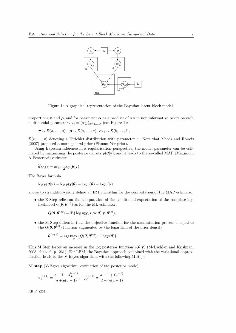
Figure 1: A graphical representation of the Bayesian latent block model.

proportions π and ρ, and for parameter α as a product of g×m non informative priors on eachmultinomial parameter αk` = (αhk`)h=1,...,r (see Figure 1):

π ∼ D(a, . . . , a), ρ ∼ D(a, . . . , a), αk` ∼ D(b, . . . , b),

D(v, . . . , v) denoting a Dirichlet distribution with parameter v. Note that Meeds and Roweis(2007) proposed a more general prior (Pitman-Yor prior).

Using Bayesian inference in a regularisation perspective, the model parameter can be esti-mated by maximising the posterior density p(θ|y), and it leads to the so-called MAP (MaximumA Posteriori) estimate

θMAP = arg maxθ

p(θ|y).

The Bayes formula

log p(θ|y) = log p(y|θ) + log p(θ)− log p(y)

allows to straightforwardly define an EM algorithm for the computation of the MAP estimate:

• the E Step relies on the computation of the conditional expectation of the complete log-likelihood Q(θ,θ(c)) as for the ML estimator:

Q(θ,θ(c)) = IE(

log p(y, z,w|θ)|y,θ(c)),

• the M Step differs in that the objective function for the maximisation process is equal tothe Q(θ,θ(c)) function augmented by the logarithm of the prior density

θ(c+1) = arg maxθ

(Q(θ,θ(c)) + log p(θ)

).

This M Step forces an increase in the log posterior function p(θ|y) (McLachlan and Krishnan,2008, chap. 6, p. 231). For LBM, the Bayesian approach combined with the variational approx-imation leads to the V-Bayes algorithm, with the following M step:

M step (V-Bayes algorithm: estimation of the posterior mode)

π(c+1)k =

a− 1 + s(c+1).k

n+ g(a− 1), ρ

(c+1)` =

a− 1 + t(c+1).`

d+m(a− 1)

RR n° 8264


αhk`(c+1)

=b− 1 +

∑i,j s

(c+1)ik t

(c+1)j` yhij

r(b− 1) + s(c+1).k t

(c+1).`

,

where s(c+1)ik and t(c+1)

j` are the current conditional probabilities of the labels and s(c+1).k and t(c+1)

.` ,their sum over the lines and columns respectively, as defined in the VEM algorithm, see AppendixB. The hyperparameters a and b are acting as regularisation parameters. In this perspective, thechoice for a and b is important. It appears clearly from the updating equations of this M stepthat V-Bayes collapses to the VEM algorithm with the uniform prior a = b = 1 and involves noregularisation. And, for Jeffreys prior (a = b = 1/2), V-Bayes has a tendency to provide moreempty cluster solutions than VEM. Frühwirth-Schnatter (2011) shows the great influence of afor Bayesian inference in the Gaussian mixture context. Based on an asymptotic analysis byRousseau and Mengersen (2011) and on a thorough finite sample analysis, she advocated to takea = 4 for moderate dimension (g < 8) and a = 16 for larger dimensions to avoid empty clusters.

In Section 5, we present numerical experiments highlighting the ability of the V-Bayes algo-rithm to avoid the "empty cluster" cases encountered with the VEM algorithm.

However, as VEM, a V-Bayes algorithm could be expected to be highly dependent of its initialvalues. Thus it could be of interest to initialise V-Bayes with the solution derived from the Gibbssampler. Obviously, since Dirichlet prior distributions are conjugate priors for the multinomialdistribution, full conditional posterior distributions of the LBM parameters are closed form andGibbs sampling is easy to implement, in such way:

Gibbs sampling for the categorical LBM

1. simulation of z(c+1) according to p(z|y,w(c);θ(c)) as in SEM-Gibbs

2. simulation of w(c+1) according to p(w|y, z(c+1);θ(c)) as in SEM-Gibbs

3. simulation of π(c+1) according to

D(a+ z(c+1).1 , . . . , a+ z(c+1)

.g )

where z.k =∑i zik denotes the number of lines in line cluster k

4. simulation of ρ(c+1) according to

D(a+ w(c+1).1 , . . . , a+ w(c+1)

.m )

where w.` =∑j wj` denotes the number of columns in column cluster `

5. simulation of α(c+1)k` according to

D(b+N1k`

(c+1), . . . , b+Nr

k`(c+1))

for k = 1, . . . , g; ` = 1, . . . ,m and with

Nhk`

(c+1)=∑i,j

z(c+1)ik w

(c+1)j` yhij . (2)

As Gibbs sampling explores the whole distribution, it is subject to label switching. This problemcan be sensibly solved for the categorical LBM by using the identifiability conditions of Theorem1: these conditions define a natural order of row and column labels except on a set of parametersof measure zero. Hence, row and column labels are post processed separately after the lastiteration, by reordering them according to the ascending values of τh = αhρ and σh = π′αh

coordinates respectively, and for a given h.

Inria


4 Model selectionChoosing relevant numbers of clusters in a latent block model is obviously of crucial importance.This model selection problem is difficult for several reasons. First there is a couple (g,m) ofnumber of clusters to be selected instead of a single number. Secondly penalised likelihoodcriteria such as AIC or BIC are not directly available since computing the maximised likelihoodis not feasible. Third determining the number of statistical units of a LBM could be questionable(number of rows, number of columns, number of cells, . . .).

Fortunately, it is possible to compute the exact integrated completed loglikelihood (ICL) ofthe categorical LBM.

4.1 The Integrated Completed Loglikelihood (ICL)ICL is the logarithm of the integrated completed likelihood

p(y, z,w | g,m) =

∫Θg,m

p(y, z,w | θg,m)p(θg,m)dθg,m

where the missing data (z,w) have to be replaced by some values closely related to the modelat hand. By taking into account the missing data, ICL is focusing on the clustering view ofthe model. For this very reason, ICL could be expected to select a stable model allowing topartitioning the data with the greatest evidence (Biernacki et al., 2000).

As stated in Section 3, Dirichlet proper non informative priors are available for the categor-ical LBM and ICL can be computed without requiring asymptotic approximations. Using theconditional independence of the zs and the ws conditionally to α,π,ρ, the integrated completedlikelihood can be written

ICL = log p(z) + log p(w) + log p(y|z,w). (3)

Using now the conjugate properties of the prior Dirichlet distributions and the conditional inde-pendence of the yij knowing the latent vectors z and w and the LBM parameters, we get (seeAppendix D for a detailed proof)

ICL(g,m) = log Γ(ga) + log Γ(ma)− (m+ g) log Γ(a)

+mg(log Γ(rb)− r log Γ(b))

− log Γ(n+ ga)− log Γ(d+ma)

+∑k

log Γ(z.k + a) +∑`

log Γ(w.` + a)

+∑k,`

[(∑h

log Γ(Nhk` + b)

)− log Γ(z.kw.` + rb)

].

where z.k, w.` and Nhk` are defined as for the Gibbs sampler (see Equation 2). In practice, the

missing labels z,w have to be chosen. Following Biernacki et al. (2000), they are replaced by

(z, w) = arg max(z,w)

p(z,w|y; θ),

θ being the estimate of the LBM parameter computed from the V-Bayes algorithm initialised bythe Gibbs sampler as described in Section 3. The maximising partition (z, w) is obtained witha MAP rule after the last V-Bayes step.

RR n° 8264


4.2 Penalised information criterionBIC is an information criterion defined as an asymptotic approximation of the logarithm of theintegrated likelihood (Schwarz, 1978). The standard case leads to write BIC as a penalisedmaximum likelihood:

BIC = maxθ

log(p(y; θ))− D

2log(n),

where n is the number of statistical units and D the number of free parameters. Unfortunately,this approximation cannot be used for LBM, due to the dependency structure of the observationsy.

However, a heuristic can be stated to define BIC. BIC-like approximations of each term ofICL (Equation 3) lead to the following approximation as n and d tend to infinity:

ICL(g,m) ' maxθ

log p(y, z, w;θ)

−g − 1

2log n− m− 1

2log d

−gm(r − 1)

2log(nd). (4)

Now, following Biernacki et al. (2000), the parameter maximizing the completed likelihoodlog p(y, z, w;θ) is replaced by the maximum likelihood estimator θ:

maxθ

log p(y, z, w;θ) ' log p(y, z, w; θ)

' log p(z, w|y; θ) + log p(y; θ).

Therefore ICL is the sum of the logarithm of the conditional distribution log p(z, w|y; θ), mea-suring the assignment confidence, and a penalised likelihood. The decomposition of ICL

ICL(g,m) = log p(z, w|y; θ) + BIC(g,m) (5)

as a sum of an entropy term and BIC is classical (McLachlan and Peel (2000), 6.10.3) and,by analogy, we conjecture from (4) and (5) the following form for BIC after a straightforwardfactorisation of the penalty:

BIC(g,m) = log p(y; θ)

−gm(r − 1) + g − 1

2log n

−gm(r − 1) +m− 1

2log d. (6)

Notice that the maximum likelihood is not available and is replaced by a lower bound computedby variational approximation. This expression of BIC(g,m) highlights two penalty terms, onefor the columns and one for the rows: the statistical units can be seen to be the rows andcolumns respectively. The number of row (resp. column) free parameters takes into account theproportions π (resp. ρ) and the parameter α of the categorical conditional distribution.

BIC is known to be a consistent estimator of the order of mixture models with boundedlog likelihoods (Keribin, 2000), whereas ICL is not (Baudry, 2009). However ICL can alsobe expected to be consistent for estimating the LBM order due to a specific behaviour of theconditional distribution of the labels p(z,w|y;θ). Indeed, Mariadassou and Matias (2013) proved

Inria


that for a categorical LBM, this distribution concentrates on the actual configuration with largeprobability as soon as θ is such that α is not too far from the true value. As a consequence,relying on the MAP rule and with an estimator θ such that α is converging to the true parametervalue, log p(z, w|y; θ) vanishes for true g and m. Moreover, this non positive term may add toBIC a supplementary penalty for incorrect g or m and hence leads ICL to be also consistent toestimate the order. Notice that this conjecture needs to assume the consistency of the maximumlikelihood and the variational estimators for LBM. These results have not been proved yet forLBM as far as we know, and still remain an interesting challenge. But this conjecture is supportedby the numerical experiments of the next section where ICL outperforms BIC for low n and d,and has the same behaviour as BIC for greater values.

5 Numerical experimentsRelevant numerical experiments on both simulated and real data sets supporting the claims ofthis paper are now presented. First we analyse the ability of the Bayesian inference throughGibbs sampling to avoid the tendency of the maximum likelihood methodology through VEMor SEM-Gibbs algorithms to provide empty clusters. After a simple illustration, Monte Carloexperiments on simulated data are performed (i) to compare the behaviour of SEM-Gibbs+VEMand Gibbs+V-Bayes algorithms (ii) to analyse the influence of the hyperparameters a and b (iii)to enlighten the behaviour of model selection criteria. Then, the LBM is experimented on a realcategorical data set already used by Wyse and Friel (2012).

5.1 Escaping from an empty cluster solution with V-Bayes

This illustration is done with an easily separated data matrix produced by Lomet et al. (2012)and Lomet (2012) for the binary LBM model1, with 50 rows, 50 columns, (g,m) = (3, 3) clustersand equal mixing proportions. The left part of Figure 2 displays the three components of πalong the iterations of the VEM algorithm while the right part of Figure 2 displays them forthe V-Bayes algorithm with (a, b) = (4, 1). Both algorithms started from the same position.VEM is rapidly trapped into an empty cluster solution. But V-Bayes, for which the estimatedproportions are not smaller than a−1

g(a−1) , escapes from this empty cluster solution and finallyprovides a satisfactory solution with the real number of row clusters g = 3.

5.2 Experiments with simulated data

Monte Carlo experiments were performed to assess the ability of Bayesian inference to avoidempty cluster solutions. A binary LBM with (g,m) = (5, 4) clusters was considered with followingBernoulli parameters

α =

ε ε ε ε

1− ε ε ε ε1− ε 1− ε ε ε1− ε 1− ε 1− ε ε1− ε 1− ε 1− ε 1− ε

where ε allows to produce easily (+), moderately (++) or hardly (+++) separated mixtures, seeGovaert and Nadif (2008), and with unequal ρ = (0.1 0.2 0.3 0.4) and π = (0.1 0.15 0.2 0.25 0.3)

1The data set is available fromhttps://www.hds.utc.fr/coclustering/doku.php.

RR n° 8264


Figure 2: Evolution of π for the VEM algorithm (on left) and the V-Bayes algorithm (on right)

or equal mixing proportions. As results for equal and unequal mixing proportions were quiteanalogous, they are not both shown in the following (see Keribin et al. (2013) for a completedisplay).

Comparing SEM-Gibbs+VEM and Gibbs+V-Bayes to avoid empty cluster solutions.For each case of separation, and each sample size (n, d) = (100, 200), (150, 150), (200, 100), 500data matrices were simulated. Both algorithms were initialized with two different numbers ofclusters:

(1) the true number of clusters: (g,m) = (5, 4),

(2) more than the true number of clusters: (g,m) = (8, 8).

The hyperparameters a and b for Bayesian inference were chosen in {1, 4, 16}2\{(1, 1)}. Theresults are summarised in Tables 1-2 for unequal mixing proportions. Case (a, b) = (1, 1) corre-sponds to the SEM-Gibbs+VEM algorithm and can be compared with Gibbs+V-Bayes algorithmon higher a and b values. It clearly appears that Bayesian inference with a = 4 or 16 and b = 1is doing a good job to avoid empty cluster solutions. As expected, taking a > 1 is quite relevantin that purpose. On the contrary, it appears clearly that taking b > 1 is harmful. As noticed bya reviewer, one possible reason for this could be that taking b > 1 means that the prior weightin the Dirichlet is more focused on the centre of the simplex i.e. all category weights are equal.In this case, b > 1 puts most prior weight on equal proportions for success and failure in theBernoulli distribution. Such heavy prior weight could penalize against separation of the blockclusters i.e. this puts more prior weight on saying there is no difference in the block probabilities(i.e. all αkl close to 0.5), and so there could be more of a tendency for empty clusters and henceoverall homogeneity in the solution.

Inria


+ ++ +++

(100,200)

PPPPPab 1 4 16

1 5.4 48 83.24 0.8 2.6 30.416 1 0.8 9.4

PPPPPab 1 4 16

1 7 23.2 73.44 1.6 1.8 0.816 0.6 1 1.2

PPPPPab 1 4 16

1 16.8 18.8 74.84 2.2 2.2 0.816 1 1.2 2.6

(150,150)

PPPPPab 1 4 16

1 7.6 29.2 71.84 1 0 6.816 0.2 0.6 0.2

PPPPPab 1 4 16

1 13 11.4 62.64 0.6 0.6 0.616 0.2 1.4 0.8

PPPPPab 1 4 16

1 17.6 8.4 654 0.6 1.2 0.616 0.4 0.8 0

(200,100)

PPPPPab 1 4 16

1 13.2 20 71.84 1 0.2 1216 0.6 0.4 0.6

PPPPPab 1 4 16

1 11.8 18.4 67.64 0.4 0.8 0.416 0.4 0.8 0.2

PPPPPab 1 4 16

1 18.2 7.8 69.64 0.8 1 0.616 0 0.4 0

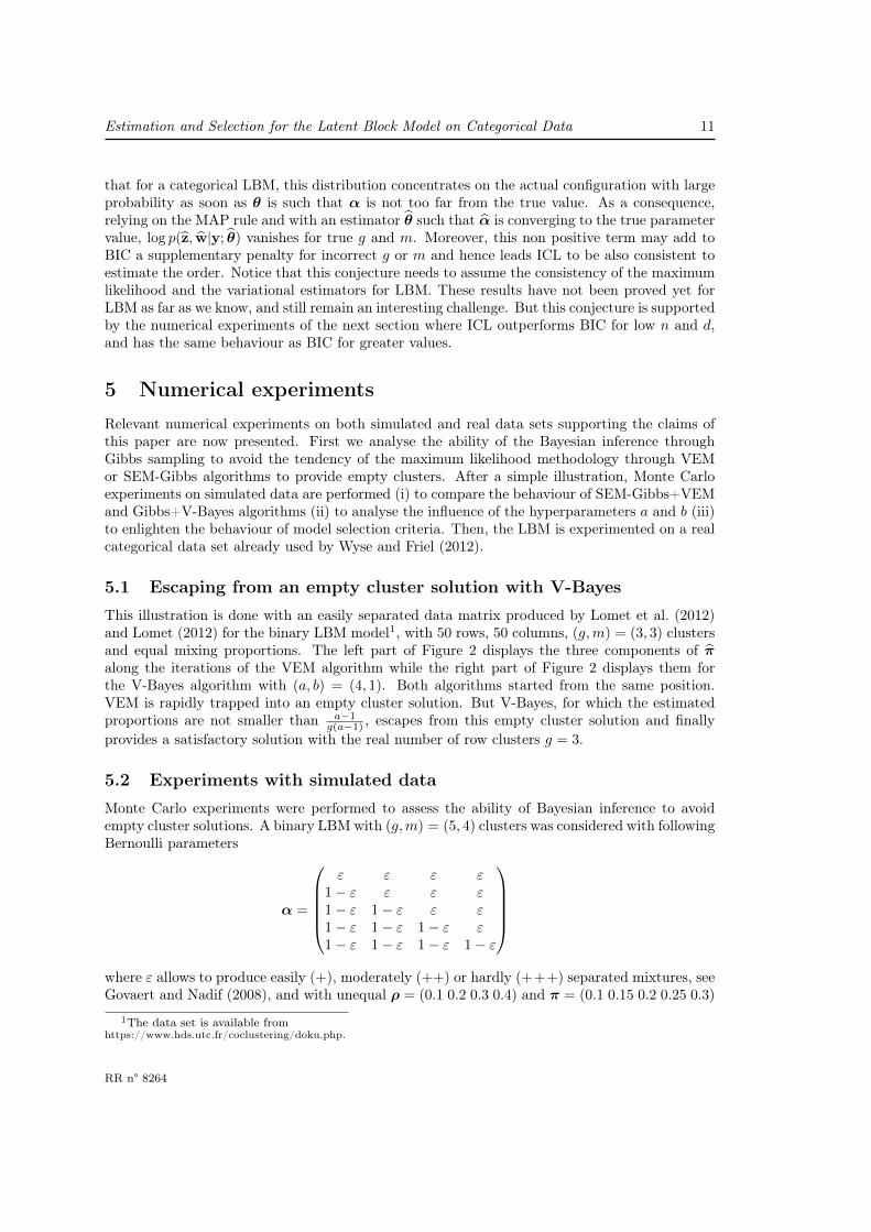
Table 1: Percentage of empty cluster solutions, for data simulated with unequal proportionmodels, obtained by SEM-Gibbs+VEM (cell a = 1, b = 1) and Gibbs+V-Bayes algorithms,called with the true (g,m), for 500 matrices in a easily separated +, moderately separated ++

and hardly separated + + + cases, for three sample sizes.

+ ++ +++

(100,200)

PPPPPab 1 4 16

1 65 96.8 1004 1.2 5.8 10016 2.2 3.8 99

PPPPPab 1 4 16

1 54.6 82.6 1004 1.8 3.6 98.216 2.4 4.4 25.2

PPPPPab 1 4 16

1 47.4 84.2 1004 3 10 97.616 5.2 13.2 31

(150,150)

PPPPPab 1 4 16

1 69.2 89 1004 0.4 1.2 10016 2.6 2.2 34

PPPPPab 1 4 16

1 54.2 64.6 1004 0.2 1.4 91.616 1.4 2.2 6

PPPPPab 1 4 16

1 57.2 69.4 1004 2.2 5.8 86.816 3 7.4 31.8

(200,100)

PPPPPab 1 4 16

1 81.4 96 1004 1.4 2.6 10016 2.2 4.6 99.2

PPPPPab 1 4 16

1 67.8 76.8 1004 1.2 2.8 9916 2.4 3 23

PPPPPab 1 4 16

1 68.2 73 1004 2.2 5.8 94.216 3.8 9 27.8

Table 2: Percentage of empty cluster solutions, for data simulated with unequal proportionmodels, obtained by SEM-Gibbs+VEM (cell a = 1, b = 1) and Gibbs+V-Bayes algorithms,called with (g,m) = (8, 8), for 500 matrices in the easily separated +, moderately separated ++

and hardly separated + + + cases, for three sample sizes.

Analysing the empty cluster solutions of SEM-Gibbs+ VEM. The fact that the SEM-Gibbs+VEM algorithm produces empty clusters can be thought of as beneficial: it could meanthat the number of clusters has been oversized and the algorithm provides a more relevant numberof clusters. To answer to this question, SEM-Gibbs+VEM was initialised with (g,m) = (8, 8)and run on 500 data sets simulated under the same conditions than previously described. Table 3reports the number of cluster finally obtained in the hardly separated cases with n = 150, d = 150and unequal mixing proportions. Results for other cases are available in Keribin et al. (2013).In all situations, the right number of clusters is chosen less than two percent of times.

Moreover, the SEM-Gibbs+VEM algorithm produces empty clusters even in case of initial

RR n° 8264


HHHHHg

m 3 4 5 6 7 8

4 0 2 0 0 0 05 1 4 4 3 2 06 0 7 13 15 6 87 0 3 12 26 23 218 0 3 13 35 85 214

Table 3: Number of provided clusters, for data simulated with the unequal proportion models,obtained by SEM-Gibbs+VEM for 500 matrices in the hardly separated + + + case with n = 150and d = 150, starting with g = 8 and m = 8.

numbers of clusters less than the real numbers. This algorithm was started with (g,m) = (8, 8)on 50 simulated binary matrix of sizes n = 50 and d = 50 of hardly separated (g,m) = (10, 10)clusters. Although the numbers of requested clusters are smaller than the right values, thealgorithm produces empty cluster solutions almost twenty percent of times (Table 4).

HHHHHg

m 6 7 8

7 1 2 188 5 64 410

Table 4: Number of provided clusters by SEM-Gibbs+VEM for 500 random initialisations in theseparated case for g = 8 and m = 8 whereas the right repartition is g = 10 and m = 10.

Analysing the behaviour of the model selection criteria. For each g and m varying fromtwo to eight, the Gibbs+V-Bayes algorithm was run on 50 simulated data sets with number ofclusters (g,m) = (5, 4) and BIC and ICL criteria were computed. Tables 5 and 6 display howmany times each (g,m) was selected in the equal mixture proportion case. The ICL criterionseems to provide a better estimation of the number of clusters than BIC, especially for thesmaller sizes of the data matrix. Otherwise, both criteria tend to choose less clusters than thereactually are in the cases where the true number of clusters is not correctly identified. Thistendency appears also on numerical experiments not reported here but available in Keribin et al.(2013) for mixtures with the same α parameters, but unequal mixing proportions. It deservesthe following comments.

First, it is worth noting that the tendency of ICL to choose fewer components than the truenumber of components of a mixture is well-known. The purpose of ICL is to assess the numberof mixture components that leads to the best clustering and it can happen that the number ofclusters is smaller than the number of mixture components. This is because a cluster may bebetter represented by a mixture of components than by a single component (see Biernacki et al.(2000) or Baudry et al. (2010)). For the LBM as mentioned in Section 4.2, when computingBIC, the maximum likelihood is approximated by the maximum free energy. The tendency ofBIC to underestimate the true number of components could indicate that the difference betweenthe maximum likelihood and the maximum free energy increases with the number of mixturecomponents. As expected, for large sizes, the performances of both criteria improve and thedifference between ICL and BIC decreases. This is in agreement with the conjecture presented

Inria


in Section 4.2.

+ ++ +++

(100,200)

4 5 6345 34 46 117 1

2 3 4 534 125 8 23 26 47 1

2 3 4 53 74 3 335 7 067

(150,150)

4 5 6345 35 3 16 11

2 3 4 534 1 185 2 296

2 3 4 53 114 32 15 1 56 1

(200,100)

4 5 6345 41 4 16 4

2 3 4 53 1 14 16 55 1 25 16

2 3 4 53 5 24 36 45 2 16

(500,1000)

4 5 645 386 117 1

2 3 4 545 446 57 1

2 3 4 54 105 2 366 17 1

(750,750)

4 5 645 456 5

2 3 4 545 44 36 3

2 3 4 54 85 406 2

(1000,500)

4 5 645 45 46 1

2 3 4 54 15 43 66

2 3 4 54 55 43 26

Table 5: The frequency of the models selected by the ICL criterion in the easily separated +,moderately separated ++ and ill separated + + + cases with equal proportion for different matrixsizes.

5.3 Congressional voting in US senateThe combination Gibbs+V -Bayes was tested on UCI Congressional Voting Records data set2recording the votes (’yes’, ’no’, ’abstained or absent’) of 435 members of the 98th congress on 16different key issues. This data set involves homogeneous 3-level categorical data.

2Congressional Voting Records data set is available fromhttp://archive.ics.uci.edu/ml/datasets/Congressional+Voting+Records.

RR n° 8264


+ ++ +++

(100,200)

3 4 5345 2 34 56 9

2 3 4 534 1 30 15 12 66

2 3 4 53 124 4 345 06

(150,150)

3 4 534 15 35 26 12

2 3 4 53 14 2 425 1 46

2 3 4 53 22 24 255 16

(200,100)

3 4 534 45 416 5

2 3 4 53 3 14 36 25 86

2 3 4 53 13 54 325 06

(500,1000)

3 4 545 38 16 117

2 3 4 545 456 47 1

2 3 4 54 15 1 456 27 1

(750,750)

3 4 545 456 5

2 3 4 545 446 6

2 3 4 54 85 396 3

(1000,500)

3 4 545 45 26 3

2 3 4 545 43 16 6

2 3 4 54 45 43 16 2

Table 6: The frequency of the models selected by the BIC criterion in the easily separated +,moderately separated ++ and ill separated + + + cases with equal proportion for different matrixsizes.

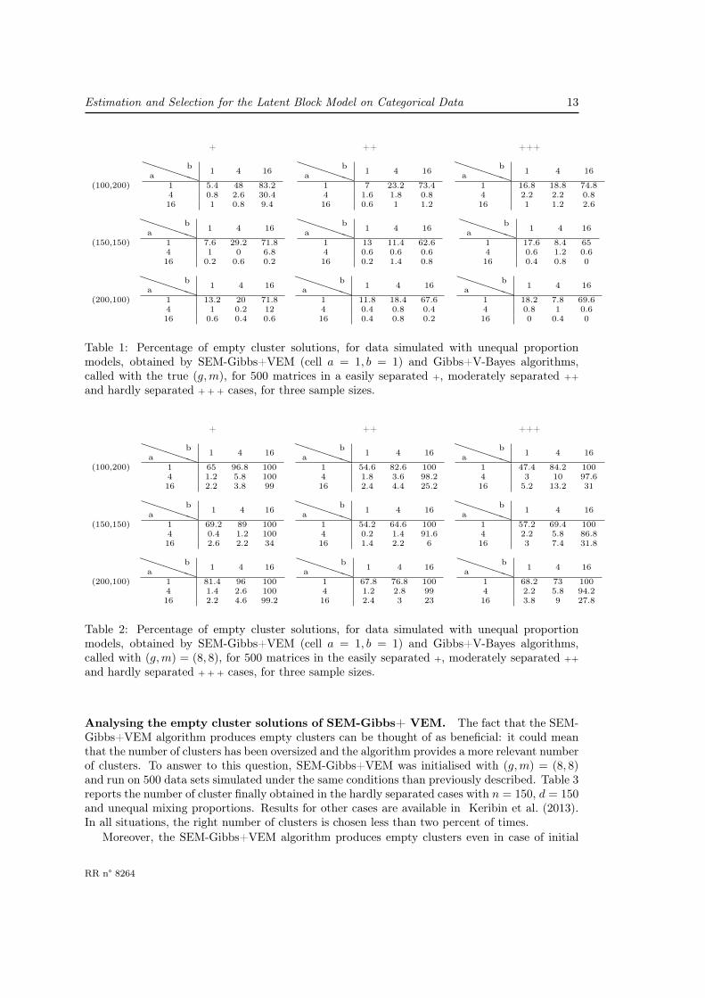
The Gibbs+V-Bayes algorithm was run on the 3-level data with (a, b) = (4, 1) and the ICL andBIC criteria were computed to select the number of clusters.ICL selected (g,m) = (5, 7) clusters, while BIC selected (g,m) = (4, 6). The rows and columnsreorganisation derived from the block clustering for each criterion is displayed in Figure 3 where’yes’ is coloured in black, ’no’ in white and ’abstained or absent’ in grey.Row cluster composition by Party is shown in Table 7. Roughly speaking, the first three clustersselected with both criteria are the same. Row cluster 1 is mainly Republican while row cluster3 is mainly Democrat. Row cluster 2 is mixed. Cluster 4 selected with BIC is split into twoclusters (4 and 5) in the model selected with ICL (the six bigger abstainers are isolated in cluster5).

Inria


ICL Rep Dem Total1 132 22 1542 25 68 933 1 162 1634 2 4 65 8 11 19

BIC Rep Dem Total1 131 24 1552 27 73 1003 1 163 1644 9 7 15

Table 7: Repartition of Democrats and Republicans for each criterion.

Figure 3: Reorganisation of the data by the ICL criterion (on left) and by the BIC criterion (onright).

The first four column clusters selected with both criteria are identical. Column clusters 1 and2 contain the issues on which Republicans voted ’yes’ and Democrats ’no’. These two columnclusters only differ for the vote of congress members belonging to row cluster 2. In contrast,column clusters 3 and 4 contain the issues on which Republicans voted ’no’ and Democrats ’yes’.Moreover, both criteria isolated in a specific cluster the issue characterised by a high level ofabstainers. Column cluster 5 selected with BIC is split into two column clusters (5 and 6) in themodel selected with ICL, due to one issue more subject to abstention.

This data set was already studied by Wyse and Friel (2012) where the ’no’ and ’abstained orabsent’ were aggregated in order to work on binary data. Assuming that g and m were random,Wyse and Friel used a collapsed sampler which marginalises over the model parameters withuniform prior (i.e. (a, b) = (1, 1) in Figure 1) aiming to compute the distribution of the mostvisited models and the maximum a posteriori cluster membership (z,w). This maximisation is

RR n° 8264


analogous to maximising the ICL criterion because :

log p(z,w, g,m|y) = ICL(z,w, g,m)

+ log p(g,m)− log p(y). (7)

Since the prior on g and m was taken to be uniform, the two algorithms should give the sameoptimal quadruplet (z,w, g,m). Wyse and Friel gave the a posteriori distribution for (g,m) butdid not provide the maximum a posteriori cluster membership (z,w). We computed it by runningtheir collapsed sampler with 110 000 iterations, 10 000 of them as burn-in iterations3. This ledto (g,m) = (6, 11) clusters (which is not in their 60% confidence level) with a correspondingICL = −3565. Replicating 30 times gave variations from 10 to 14 column clusters, with 6 rowclusters each time, and corresponding ICLs were computed. The best ICL value was −3554 for(g,m) = (6, 13). Running Gibbs+V-Bayes on the same binary data set and the same priorsselected (g,m) = (5, 13) clusters with corresponding ICL= −3553. Notice that ICL(g,m) isquite flat around its maximum. The results are similar, requiring six times more iterations forthe collapsed sampler.

6 Discussion

In this paper, we show that Bayesian inference through Gibbs sampling is beneficial to pro-duce regularised estimates of the LBM for categorical data. A sufficient solution to ensure theidentifiability of the LBM for categorical data has been provided. Contrary to the VEM orV-Bayes algorithms, the SEM-Gibbs algorithm and Gibbs sampling provide solutions not highlydependent of the starting values. Restricting attention to point estimation, Bayesian inferencethrough Gibbs sampling from non informative priors produces regularised parameter estimation.The solution providing the posterior mode of the parameters is not suffering the label switchingproblem and can be used as initial values of the V-Bayes algorithm, and thus avoid the emptycluster solutions which jeopardizes maximum likelihood inference for the LBM. Moreover, takingprofit of the exhibited sufficient condition ensuring the identifiability of the LBM for categoricaldata, it is possible to define a natural order to post process the rows and columns after Gibbssampling in order to deal with the label switching problem in a proper way. On the other hand,we select a latent block model using the integrated completed likelihood ICL which can be com-puted without requiring asymptotic approximations. A good perspective for future work wouldbe to prove the conjecture stated in Section 4.2: namely ICL criterion provides a consistent es-timation of the number of clusters (g,m) for the LBM, contrary to the standard mixture modelfor which ICL is not consistent. Otherwise, an alternative is to use the collapsed sampler ofWyse and Friel (2012). Maximising the posterior collapsed is closely related to maximising ICLfor flat (g,m) priors (see equation 7). In our experiments, ICL appears to be efficient to findthe (z,w, g,m) maximising the posterior log p(z,w, g,m|y) and less computationally demandingthan the collapsed sampler. But, the latter is able to explore the uncertainty in the joint supportof all models and corresponding missing labels. A perspective would be to analyse the variabilityof ICL with a random sampling of (z,w) according to the distribution p(z,w; θ). Preliminarynumerical experiments on simulated data show that the variability of ICL depends on (g,m) andis clearly more important for g or m greater than the real values. It could be an interestingsubject for further research.

3The code of Wyse and Friel is available athttp://www.ucd.ie/statdept/jwyse.

Inria


Acknowledgements The authors thank the reviewers and the Associate Editor for their veryhelpful comments which have greatly improved this paper. C. K. has been supported by LMH(Hadamard Mathematics Labex), backed by the foundation FMJH (Fondation MathématiqueJacques Hadamard).

RR n° 8264


AppendicesA Proof of Theorem 1The identifiability of a parametric model requires that for any two different values θ 6= θ′ inthe parameter space, the corresponding probability distribution IPθ and IPθ′ are different. Weprove that, under assumptions of Theorem 1, there exists a unique parameter θ = (π,ρ,α), upto a permutation of row and column labels, corresponding to IP(y) the probability distributionfunction of matrix y having at least 2m− 1 rows and 2g− 1 columns. The proof is adapted fromCelisse et al. (2012) who set up a similar result for the Stochastic Block Model. Notice first thatτ = Aρ is the vector of the probability τk to have 1 in a cell of a row of given row class k:

τk = IP(yij = 1|zik = 1) =∑`

ρ`αk` = (Aρ)k.

As all the coordinates of τ are distinct, R defined as the g× g matrix of coefficients Rik = (τk)i,for 0 ≤ i < g and 1 ≤ k ≤ g, is Vandermonde, and hence invertible. Consider now ui, theprobability to have 1 on the i first cells of the first row of y:

ui = IP(y11 = 1, . . . , y1i = 1)

=∑

k,`1,...,ì

IP(z1k = 1)×

j=i∏j=1

(IP(y1j |z1k = 1, wj`j = 1)IP(wj`j = 1)

)=

∑k

IP(z1k = 1)×∑`1

IP(y11|z1k = 1, w1`1 = 1)IP(w1`1 = 1)×

. . .×∑ì

IP(y1i|z1k = 1, wiì = 1)IP(wiì = 1)

= IP(y11 = 1, . . . , y1i = 1) =∑k

πk(τk)i

With a given IP(y), u1, . . . , u2g−1 are known, and we denote u0 = 1. Let now M be the(g + 1) × g matrix defined by Mij = ui+j−2, for all 1 ≤ i ≤ g + 1 and 1 ≤ j ≤ g and define Mi

as the square matrix obtained by removing the row i from M . The coefficients of M are

Mij = ui+j−2 =∑

1≤k≤g

τ i−1k πkτ

j−1k .

We can write, with Aπ = Diag(π)

Mg = RAπR′.

Now, R, unknown at this stage, can be retrieved by noticing that the coefficients of τ are theroots of the following polynomial (Celisse et al., 2012) of degree g

B(x) =

g∑k=0

(−1)k+gDkxk,

Inria


where Dk = detMk and Dg 6= 0 as Mg is a product of invertible matrices. Hence, it is possibleto determine τ , and R is now known. Consequently, π is defined in a unique manner by Aπ =R−1MgR

′−1.In the same way, ρ is defined in a unique manner by considering the probabilities σ` to have 1in a column of column class ` and the probabilities vj to have 1 on the j first cells of the firstcolumn of y

σ` = IP(yij = 1|wj` = 1) and vj = IP(y11 = 1, . . . , yj1 = 1)

To determine α, we introduce for 1 ≤ i ≤ g and 1 ≤ j ≤ m the probabilities Uij to have 1 ineach i first cells of the first row and in each j first cells of the first column

Uij = IP(y11 = 1, . . . , y1i = 1, y21 = 1, . . . , yj1 = 1)

=∑

k,`1,`2,...,`i,

k1,...,kj

IP(y11|z1k = 1, w1` = 1)×

IP(z1k = 1)IP(w1` = 1)×i∏

λ=2

IP(y1λ|z1k = 1, wλ`λ = 1)IP(wλ`λ = 1)×

j∏η=2

IP(yη1|zηkη = 1, w1` = 1)IP(zηkη = 1)

=∑k,`

IP(y11|z1k = 1, w1` = 1)IP(z1k = 1)×

IP(w1` = 1)IP(y1i|z1k = 1)i−1IP(yj1|w1` = 1)j−1

=∑k,`

πkτi−1k αk`ρ`σ

j−1` .

These probabilities are known and we can write, with Sj` = (σ`)j−1, j = 1, . . .m, ` = 1, . . . ,m

U = RAπAAρS′,

and it leads to define A = A−1π R−1US

′−1A−1ρ , and hence α, in a unique manner.

The proof is straightforwardly extended to the categorical case. The identification of π andρ are obtained by considering the probabilities of yij = 1 where 1 is the first outcome of themultinomial distribution. Then, each Ah = (αhk`)k=1,...,g;`=1,...,m is successively identified byconsidering yij = `, i = 1, . . . ,m, j = 1, . . . , g.

B VEM algorithm for categorical dataGovaert and Nadif (2008) proposed to use, for the binary case, a variational approximation of theEM algorithm by imposing that the joint distribution of the labels takes the form q

(c)zw(z,w) =

q(c)z (z)q

(c)w (w). To get simpler formulas, we will denote

s(c)ik = q(c)

z (zik = 1)

and

t(c)j` = q(c)

w (wj` = 1).

RR n° 8264


Using the variational approximation, the maximisation of the loglikelihood is replaced by themaximisation of the free energy

F(qzw,θ) = IEqzqw

[log

p(y, z,w;θ)

qz(z)qw(w)

]alternatively in qz, qw and θ (see Keribin, 2010). The difference between the maximum loglikeli-hood and the maximum free energy is the Kullback divergenceKL(qzw||p(z,w|y;θ)) = IEqzw

[log qzw(z,w)

p(z,w|y;θ)

]. This can be extended to the categorical LBM,

and leads to the following Variational EM (VEM) algorithm:

E step It consists of maximising the free energy in qz and qw, and it leads to:

1. Computing s(c+1)ik with fixed w(c)

jl and θ(c)

s(c+1)ik =

π(c)k ψk(yi·;α

(c)k· )∑

k′ π(c)k′ ψ

(c)k′ (yi·;α

(c)k′·)

, k = 1, . . . , g

where yi· denotes the row i of the matrix y,αk· = (αk1, . . . , αkm), and

ψk(yi·;α(c)k· ) =

∏`,h

(αhk`(c)

)∑j t

(c)j` y

hij

2. Computing t(c+1)jl with fixed s(c+1)

ik and θ(c)

t(c+1)j` =

ρ(c)` φ`(y·j ;α

(c)·` )∑

`′ ρ(c)`′ φ`′(y·j ;α

(c)·`′ )

, ` = 1, . . . ,m

where y·j denotes the column j of the matrix y, α·` = (α1`, . . . , αg`) and

φ`(y·j ;α(c)·` ) =

∏k,h

(αhk`(c)

)∑i s

(c+1)ik yhij .

M step Updating θ(c+1). Denoting s(c+1).k =

∑i s

(c+1)ik ,

t(c+1).` =

∑j t

(c+1)j` , it leads to

π(c+1)k =

s(c+1).k

n,

ρ(c+1)` =

t(c+1).`

d,

αhk`(c+1)

=

∑i,j s

(c+1)ik t

(c+1)j` yhij

s(c+1).k t

(c+1).`

.

Inria


C SEM algorithm for categorical dataE and S step

1. computation of p(z|y,w(c);θ(c)),then simulation of z(c+1) according top(z|y,w(c);θ(c)):

p(zi = k|yi·,w(c);θ(c)) =π

(c)k ψk(yi·;α

(c)k· )∑

k′ π(c)k′ ψ

(c)k′ (yi·;α

(c)k′·)

,

for k = 1, . . . , g with

ψk(yi·;αk·) =∏`,h

(αhk`(c)

)∑j w

(c)j` y

hij

2. computation of p(w|y, z(c+1);θ(c)),then simulation of w(c+1) according top(w|y, z(c+1);θ(c)).

M step Denoting z.k :=∑i zik and w.` :=

∑j wj`, it leads to

π(c+1)k =

z(c+1).k

n, ρ

(c+1)` =

w(c+1).`

d

and

αhk`(c+1)

=

∑i,j z

(c+1)ik w

(c+1)j` yhij

z(c+1).k w

(c+1).`

.

Note that the formulae of VEM and SEM-Gibbs are essentially the same, except that theprobabilities sik and tj` are replaced with binary indicator values zik and wj`.

D Computing ICLIn this section, the exact ICL expression is derived for categorical data. Using the conditionalindependence of the zs and the ws conditionally to α,π,ρ, the integrated completed likelihoodcan be written

p(y, z,w) =

∫p(y, z,w,α,π,ρ)p(α)p(π)p(ρ)dαdπdρ

=

∫p(y|z,w,α,π,ρ)p(z,w|α,π,ρ)×

p(α)p(π)p(ρ)dαdπdρ

=

∫p(y|z,w,α)p(α)dα×∫p(z|π)p(π)dπ

∫p(w|ρ)p(ρ)dρ

= p(z)p(w)p(y|z,w).

RR n° 8264


Thus

ICL = log p(z) + log p(w) + log p(y|z,w).

Now, according to the LBM definition,

p(z|π) =∏i,k

πzikk .

Since the prior distribution of π is the Dirichlet distribution D(a, . . . , a)

p(π) =Γ(ga)

Γ(a)g

∏k

πa−1,

we have

p(π|z) =p(z|π)p(π)∫p(z|π)p(π)

∝∏k

πz.k+a−1k .

We recognise a non-normalised Dirichlet distributionD(z.1 + a, . . . , z.g + a) with the normalising factor

Γ(n+ ga)∏k Γ(z.k + a)

.

The expression of p(z) directly follows from the Bayes theorem

p(z) =Γ(ag)

Γ(a)g

∏k Γ(z.k + a)

Γ(n+ ag). (8)

In the same manner,

p(w) =Γ(am)

Γ(a)m

∏` Γ(w.` + a)

Γ(d+ am). (9)

We now turn to the computation of p(y|z,w). Since α and (z,w) are independent, we have

p(α|y, z,w) =p(y|z,w,α)p(α)∫p(y|z,w,α)p(α)dα

,

and, using the conditional independence of yij knowing z, w and α,

p(y|z,w,α) =∏i,j,k,`

(∏h

(αhk`)yhij

)zikwj`

=∏k,`

(∏h

(αhk`)∑i,j zikwj`y

hij

)

=∏k,`

(∏h

(αhk`)Nhk`

).

Inria


Therefore

p(α|y, z,w) ∝∏k,`

(p(αk`)

∏h

(αhk`)Nhk`

)

∝∏k,`

[(∏h

(αhk`)b−1

)(∏h

(αhk`)Nhk`

)]

∝∏k,`

(∏h

(αhk`)b+Nhk`−1

).

because p(αk`) is the density of a Dirichlet distributionD(b, . . . , b). Each term k`, is the density of a non-normalised Dirichlet distribution D(b +N1k`, . . . , b+Nr

k`) with the normalising factor

Γ(z.kw.` + rb)∏h Γ(Nh

k` + b).

Thus, by the Bayes formula,

p(y|z,w) =∏k,`

Γ(rb)

Γ(b)r

∏h Γ(Nh

k` + b)

Γ(z.kw.` + rb). (10)

And, the ICL criterion, presented in Section 4.1, is straightforwardly derived from equations (3),(8), (9) and (10).

ReferencesAllman, E., Mattias, C., and Rhodes, J. (2009). Identifiability of parameters in latent structuremodels with many observed variables. The Annals of Statistics, 37:3099–3132.

Banerjee, A., Dhillon, I., Ghosh, J., Merugu, S., and Modha, D. S. (2007). A generalizedmaximum entropy approach to bregman co-clustering and matrix approximation. Journal ofMaching Learning Research, 8:1919–1986.

Baudry, J.-P. (2009). Sélection de modèle pour la classification non supervisée. Choix du nombrede classes. PhD thesis, Université Paris Sud.

Baudry, J.-P., Raftery, A., Celeux, G., Lo, K., and Gottardo, R. (2010). Combining MixtureComponents for Clustering. Journal of Computational and Graphical Statistics, 19:332–353.

Biernacki, C., Celeux, G., and Govaert, G. (2000). Assessing a mixture model for clustering withthe integrated completed likelihood. IEEE Transactions on Pattern Analysis and MachineIntelligence, 22:719–725.

Biernacki, C., Celeux, G., and Govaert, G. (2010). Exact and monte carlo calculations of in-tegrated likelihoods for the latent class model. Journal of Statistical Planning and Inference,140:2991–3002.

Carreira-Perpiñàn, M. and Renals, S. (2000). Practical identifiability of finite mixtures of mul-tivariate bernoulli distributions. Neural Computation, 12:141–152.

RR n° 8264


Celeux, G. and Diebolt, J. (1985). Stochastic versions of the em algorithm. ComputationalStatistics Quaterly, 2:73–82.

Celisse, A., Daudin, J.-J., and Latouche, P. (2012). Consistency of maximum-likelihood andvariational estimators in the stochastic block model. Electron. J. Statist., 6:1847–1899.

Daudin, J.-J., Picard, F., and Robin, S. (2008). A mixture model for random graphs. Statisticsand Computing, 18:173–183.

Dempster, A. P., Laird, N. M., and Rubin, D. B. (1977). Maximum likelihood from incompletedata via the EM algorithm (with discussion). Journal of the Royal Statistical Society, SeriesB, 39:1–38.

Frühwirth-Schnatter, S. (2006). Finite mixture and Markov switching models. Springer series instatistics. Springer.

Frühwirth-Schnatter, S. (2011). Mixtures : estimation and applications, chapter Dealing withlabel switching under model uncertainty, pages 193–218. Wiley.

Govaert, G. (1977). Algorithme de classification d’un tableau de contingence. In First interna-tional symposium on data analysis and informatics, pages 487–500, Versailles. INRIA.

Govaert, G. (1983). Classification croisée. PhD thesis, Université Paris 6, France.

Govaert, G. and Nadif, M. (2008). Block clustering with bernoulli mixture models: Comparisonof different approaches. Computational Statistics and Data Analysis, 52:3233 – 3245.

Govaert, G. and Nadif, M. (2010). Latent block model for contingency table. Communicationin Statistics - Theory and Methods, 39:416 – 425.

Gyllenberg, M., Koski, T., Reilink, E., and Verlann, M. (1994). Non-uniqueness in probabilisticnumerical identification of bacteria. Journal of Applied Probability, 31:542–548.

Jagalur, M., Pal, C., Learned-Miller, E., Zoeller, R. T., and Kulp, D. (2007). Analyzing insitu gene expression in the mouse brain with image registration, feature extraction and blockclustering. BMC Bioinformatics, 8:S5.

Keribin, C. (2000). Consistent estimation of the order of mixture models. Sankhya Series A,62:49–66.

Keribin, C. (2010). Méthodes bayésiennes variationnelles: concepts et applications en neuroim-agerie. Journal de la Société Française de Statistique, 151:107–131.

Keribin, C., Brault, V., Celeux, G., and Govaert, G. (2012). Model selection for the binary latentblock model. Proceedings of COMPSTAT 2012.

Keribin, C., Brault, V., Celeux, G., and Govaert, G. (2013). Estimation and Selection for theLatent Block Model on Categorical Data. Rapport de recherche RR-8264, INRIA.

Lomet, A. (2012). Sélection de modèle pour la classification croisée de données continues. PhDthesis, Université de Technologie de Compiègne.

Lomet, A., Govaert, G., and Grandvalet, Y. (2012). Un protocole de simulation de données pourla classification croisée. In 44ème journées de statistique, Bruxelles.

Inria


Madeira, S. C. and Oliveira, A. L. (2004). Biclustering algorithms for biological data analysis:A survey. IEEE/ACM Transactions on Computational Biology and Bioinformatics, 1:24–45.

Mariadassou, M. and Matias, C. (2013). Convergence of the groups posterior distribution inlatent or stochastic block models. arXiv preprint arXiv:1206.7101v2.

McLachlan, G. J. and Krishnan, T. (2008). The EM algorithm and extensions. Wiley, Nex York,2nd edition.

McLachlan, G. J. and Peel, D. (2000). Finite Mixture Models. Wiley, Nex York.

Meeds, E. and Roweis, S. (2007). Nonparametric bayesian biclustering. Technical Report UTMLTR 2007-001, Department of Computer Science, University of Toronto.

Nobile, A. and Fearnside, A. T. (2007). Bayesian finite mixtures with an unknown number ofcomponents: The allocation sampler. Statistics and Computing, 17:147–162.

Rousseau, J. and Mengersen, K. (2011). Asymptotic behaviour of the posterior distribution inoverfitted models. Journal of the Royal Statistical Society, 73:689–710.

Schwarz, G. (1978). Estimating the dimension of a model. The Annals of Statistics, 6(2):461–464.

Shan, H. and Banerjee, A. (2008). Bayesian co-clustering. In Proceedings of the 2008 EighthIEEE International Conference on Data Mining, ICDM ’08, pages 530–539, Washington, DC.IEEE Computer Society.

Wyse, J. and Friel, N. (2012). Block clustering with collapsed latent block models. Statistics andComputing, 22:415–428.

RR n° 8264

RESEARCH CENTRESACLAY – ÎLE-DE-FRANCE

1 rue Honoré d’Estienne d’OrvesBâtiment Alan TuringCampus de l’École Polytechnique91120 Palaiseau

PublisherInriaDomaine de Voluceau - RocquencourtBP 105 - 78153 Le Chesnay Cedexinria.fr

ISSN 0249-6399

estimation and selection for the latent block model on

Documents