estimating visitation in national parks and other … · each type of sampling, we provide formulas...

ESTIMATING VISITATION IN NATIONAL PARKS AND OTHER PUBLIC LANDS1

Christopher G. Leggett, Ph.D.2

Bedrock Statistics, LLC3 25 Bridget Circle

Gilford, NH 03249 (603) 892-1064

[email protected]

April 13, 2015

1 This report was prepared for Heather Best, National Park Service, Environmental Quality Division, by Bioeconomics, Incorporated, 315 South 4th Street, East Missoula, MT, 59801, under Award Number P13PD02250.

2 A number of individuals provided helpful comments on earlier drafts of this report, including David Paterson (University of Montana), Chris Neher (Bioeconomics, Incorporated), John Duffield (Bioeconomics, Incorporated), Rachel Bouvier (rbouvier consulting LLC), Matthew Zafonte (California Department of Fish and Wildlife), Michael Welsh (Industrial Economics, Incorporated), Dan Cokewood (Kean University), and David Henry (Industrial Economics, Incorporated). Randall Bennett was responsible for graphic design.

3 Much of the expertise required to develop this report was obtained while the author was conducting applied visitor count studies for the National Park Service, the National Oceanic and Atmospheric Administration, the U.S. Fish and Wildlife Service, and various states with Mark Curry, Nora Scherer, Robert Unsworth, and Robert Paterson as a Senior Associate at Industrial Economics, Incorporated.

ii

EXECUTIVE SUMMARY

While obtaining visitation estimates is straightforward at parks that require all visitors to pay a fee and pass through a main entrance, there are many parks that deviate substantially from this ideal. In these situations, one faces difficult decisions with regard to the allocation of field effort, as it is typically prohibitively expensive to continuously count visitors at numerous entrances over long time periods. Random sampling of days and entrances can reduce costs, but this introduces statistical complexity and sampling error. Alternatively, automated vehicle or pedestrian counters can be installed at visitor entrances, but counters must be carefully deployed, monitored, and calibrated. Off-site surveys can be used to develop visitation estimates, but the development and implementation of off-site surveys requires a specialized set of skills.

Given these challenges, selecting and implementing an appropriate visitor count methodology at any given park requires a unique combination of (1) detailed, park-specific knowledge, and (2) technical expertise in several somewhat disparate fields, including statistical sampling, traffic engineering, and survey design. While excellent reference texts exist within each of these fields, they are often somewhat inaccessible to non-experts and they do not focus on park visitation. This report aims to provide a comprehensive overview of methods for estimating park visitation, extracting relevant information from related fields and presenting it in a manner that is accessible to researchers and park personnel.

Although park visitation estimates may be useful in a variety of contexts, this report is primarily intended to inform efforts to develop visitation estimates for natural resource damage assessments. Natural resource damage assessments (NRDAs) are conducted by government agencies at sites where natural resources may have been injured due to a release of oil or hazardous substances. These injuries can lead to recreational losses at parks when the value that the public derives from the park is reduced due to a temporary closure or advisory. Assessments of recreational losses in NRDAs typically require an estimate of the change in recreational trips resulting from the closure/advisory.

The report is divided into four chapters:

Chapter 1: Overview of Statistical Sampling Techniques: Chapter 1 provides an overview of four sampling approaches frequently applied in studies designed to obtain park visitation estimates: simple random sampling, stratified random sampling, cluster sampling, and systematic sampling. For each type of sampling, the intuition and mathematics are explained in detail (including formulas for estimating the population total and its variance), and a concrete example is provided. The chapter concludes with a brief overview of ratio estimation and sampling weights.

Chapter 2: On-Site Counts by Field Personnel: Chapter 2 provides an overview of available methodologies for implementing on-site count studies. The emphasis is primarily on methodologies that involve departure counts at site entrances. The chapter begins by discussing simple designs where time periods are randomly sampled and all entrances are monitored by field personnel during every selected time period. It then allows for random

iii

sampling of one or more entrances in addition to time periods. The chapter concludes with a discussion of instantaneous on-site counts such as airplane overflights.

Chapter 3: Automated Counters: Chapter 3 describes the use of automated counters and video cameras to estimate visitation in parks. The chapter begins with an overview of the automated count process, including technical and practical challenges that arise with a variety of devices. It then provides a detailed description of available technologies, describing advantages and disadvantages associated with each. The chapter concludes with summary recommendations for specific visitor count contexts, such as unpaved trails, paved paths/trails, and entrance roads.

Chapter 4: Off-Site Surveys: This chapter describes the use of off-site surveys to develop trip estimates. The chapter begins by discussing the types of situations where an off-site survey is likely to be useful. This discussion is followed by a brief comparison of the sampling contexts for on-site counts versus off-site surveys. Next, a detailed description of the steps required to implement an off-site survey is provided. The chapter concludes with a discussion of several challenges specific to off-site surveys: nonresponse bias, recall error, and cell-only households.

iv

CONTENTS

Page Chapter 1: Overview of Statistical Sampling Techniques 1 Sampling Concepts 1 Simple Random Sampling 7 Stratified Random Sampling 13 Cluster Sampling 22 Systematic Sampling 29 Ratio Estimation 32 Sampling Weights 38 Chapter 2: On-Site Counts by Field Personnel 40 Overview 40 Selecting Days for On-Site Counts 42 Simple Departure Counts 45 Departure Counts with Sampling of Shifts 49 Departure Counts with Sampling of a Single Entrance 55 Departure Counts with Sampling of Multiple Entrances 59 Instantaneous Counts 61

Chapter 3: Automated Counters 66 Counter Installation and Monitoring 67 Counter Calibration 70 Data Recording and Transmission 72 Automated Counter Technologies 75 Summary and Recommendations 88

v

Chapter 4: Off-Site Surveys 91 Conditions Favoring Off-Site Surveys 92 The Sampling Context for Off-Site Surveys 94 Developing and Implementing an Off-Site Survey 96 Nonresponse Bias 116 Recall Error 122 Incorporating Cell Phones 124

References 129

1

CHAPTER 1

OVERVIEW OF STATISTICAL SAMPLING

TECHNIQUES

This chapter provides an overview of statistical techniques that underlie attempts to estimate visitation at national parks and other public lands. At its core, estimating visitation is a statistical sampling problem. With the exception of the very simplest of parks, it is typically infeasible to directly count every single visitor that enters a park. Consequently, it is necessary to sample visitors in some way, then extrapolate from the sample to obtain an estimate of visitation. This chapter discusses a variety of ways in which visitors can be sampled, laying out the intuition and the mathematics underlying each sampling technique.1

We begin by introducing basic sampling concepts and terminology. We then describe four different approaches to sampling that are frequently applied in studies designed to obtain visitation estimates: simple random sampling, stratified random sampling, cluster sampling, and systematic sampling. For each type of sampling, we provide formulas for estimating the population mean and the population total, including standard errors. The chapter concludes with a brief overview of ratio estimation and sampling weights.

SAMPLING CONCEPTS

The sampling unit is the individual item that we wish to measure, the population is the overall collection of sampling units that we would like to characterize, and the process of drawing a sample involves selecting a subset of sampling units from the population for careful examination. Suppose, for

1 The report borrows heavily from introductory sampling texts such as Lohr (1999) and Cochran (1977), which do an excellent job in laying out the theory and intuition underlying sampling techniques. Readers interested in additional detail are urged to consult those texts.

Chapter 1: Overview of Statistical Sampling Techniques

2

example, that we wanted to conduct a mail survey of licensed anglers in Washington State to determine the total number of fishing trips taken by in-state anglers to Lake Roosevelt. In this case, each licensed angler would be a sampling unit, the population would be the set of all licensed anglers in the state, and the subset of anglers that we contact to obtain trip information would be the sample.

It is important to clearly define the sampling units and population in any visitation study. In addition, despite the common use of the term “population,” it is important to note that the definition for population considered here does not necessarily always involve people – it could involve trips, time periods, or geographic areas. With on-site studies of visitation (e.g., on-site visitor counts at entrances), the population is often the set of all days within a season or year, and the sampling unit is a single day. In contrast, with off-site studies (e.g., mail surveys of the general population), the population is often defined as a set of households living within a specific geographic area, and the sampling unit is a single household.

The sampling frame is simply a comprehensive list of sampling units from which the sample is selected. In the mail survey of licensed anglers described above, the sampling frame might be the subset of licensed anglers who provided a valid address when they purchased a fishing license. In the case of a year-long on-site visitor count study, the sampling frame for selecting on-site count days might be the list of all 365 days in the year.

Ideally, the sampling frame would be identical to the population, but there are typically at least minor differences. For example, suppose we were interested in characterizing the population of Orange County, California households, and our sampling frame was a list of all Orange County residential addresses available from the U.S. Postal Service. This sampling frame excludes some households who are in our population: it excludes households that moved into the county within the last few weeks and do not yet appear in the U.S. Postal Service database. The sampling frame also includes some households who are not in our population: it would include individuals who had recently moved or passed away.

The purpose of drawing a sample is to obtain a quantitative measurement for every selected unit in order to form an estimate of a population parameter. We will use the variable “y” to represent these quantitative measurements, and we will use subscripts to denote specific units in the sample, so that the quantitative measurement associated with the first unit is represented by y1, the second unit by y2, and the ith unit by yi. For example, if we sampled five individuals and used 𝑦𝑖 to represent the weight of the ith individual, then the sample might look like this:


3

𝑦1=150 𝑦2=125 𝑦3=185 𝑦4=145 𝑦5=95

Our goal will be to use information from the sample to estimate the population mean or total for y.2 With studies designed to estimate park visitation, we are typically more interested in estimating a total than a mean. Following the notation in Cochran (1977), we denote the true population mean by �̅� and the true population total by Y, and we denote estimates of these population parameters by using “hats”:

�̂̅� and �̂�. For example, if there were 2.3 million visits to Yellowstone National park last year, but we obtained an estimate of 2.1 million visits based on counts conducted on a sample of days, then 𝑌 =

2.3 and �̂� = 2.1. 3

The population total is defined as4

𝑌 = ∑ 𝑦𝑖

𝑁

𝑖=1

= 𝑦1 + 𝑦2 + ⋯ + 𝑦𝑁

where N is the total number of sampling units in the population. The population mean is defined as

�̅� =1

𝑁∑ 𝑦𝑖

𝑁

𝑖=1

=𝑌

𝑁

The concept of sampling error is fundamental to sampling statistics and to expressions of the amount of uncertainty (e.g., standard error, confidence interval, etc.) associated with an estimate. Sampling error

is simply the difference between the estimate calculated from a specific sample (e.g., �̂�) and the true value of the population parameter (e.g., 𝑌). Sampling error will differ from one sample to another, as each sample provides a different set of y values and therefore a different estimate.

Example 1.1: Sampling Error

Suppose the population of visitors to a particular park consists of exactly ten persons, and the following dataset represents the number of times each of these ten individuals visited the park last year:

2 One might also be interested in estimating a proportion rather than a mean or total (e.g., the proportion of visitors who participate in a given activity). As this document focuses primarily on obtaining total visitation estimates, we do not provide separate formulas for proportions. However, proportions can be estimated by simply using a binary (0/1) y variable in the formulas presented herein. For example, we would estimate the proportion of units with a particular characteristics by letting y = 1 if the sampled unit has a particular characteristic and letting y = 0 if it does not. Specific formulas for proportions are presented in Lohr (1999) and Cochran (1977). 3 Note that in almost all sampling contexts, we won’t ever actually know the true values of �̅� and 𝑌. If we did, then we wouldn’t be conducting the study in the first place! 4 The Σ notation is used to denote summations across sampling units. For example, the expression ∑ 𝑦𝑖

𝑁𝑖=1

represents the sum of all values of y associated with the first through the Nth sampling units. Thus, if there are

three individuals in the population who take 5, 2, and 7 trips, then ∑ 𝑦𝑖 =𝑁𝑖=1 (𝑦1 + 𝑦2 + 𝑦3) = (5 + 2 + 7) = 16.


4

Person No. Trips

1 2 2 7 3 0 4 0 5 1 6 5 7 3 8 2 9 0

10 0

The population mean trips is �̅� = (2+7+0+0+1+5+3+2+0+0) ÷ 10 = 2.0 trips. Suppose we draw a sample of five persons, and obtain the following responses when we ask how many times each person visited the park last year: {7, 0, 1, 3, 0}. In this case, the sample average is (7+0+1+3+0) ÷ 5 or 2.2 trips. If the sample average is used to estimate the population mean, then the sampling error is 2.2 – 2.0 = 0.2 trips. The sampling error associated with three different (arbitrary) samples of five persons from this population is shown below: Sample 1: {2, 7, 5, 3, 0} Sampling error = (17/5) – 2.0 = 1.4 Sample 2: {0, 0, 1, 3, 0} Sampling error = (4/5) – 2.0 = -1.2 Sample 3: {7, 1, 2, 0, 0} Sampling error = (10/5) – 2.0 = 0.0

Due to sampling error, our estimates will differ from the population parameters that we are trying to measure. This certainly is not surprising; after all, we are only examining a sample from the population, not the entire population. Sometimes the difference will be positive, sometimes it will be negative. An estimator is described as unbiased if these positive and negative sampling errors balance out, on average. That is, the estimator is unbiased if the average sampling error is expected to be zero across a very large number of samples. Alternatively, the estimator is described as biased if the sampling error is expected to be greater or less than zero, on average.

When reporting estimates based on a sample, it is customary to provide some measure of the degree to which variability in the sampling error may impact the results. The measure that is frequently provided is the standard error. The smaller the standard error, the more precise the estimate. The formula for calculating standard error will vary depending on the sampling approach applied. As a result, standard error formulas are presented in later sections, where specific sampling approaches are discussed. However, two cross-cutting themes arise in these formulas. First, the standard error generally declines as the sample size (n) increases. Larger sample sizes provide more information about the population, allowing us to estimate population parameters with greater precision. Second, the standard error declines as population variance decreases. The population variance is a measure of how “variable” or “spread out” the data are in the population from which we are drawing the sample:


5

It is easier to obtain precise estimates of population parameters when the population has a lower variance, or is less variable. For example, we could obtain a more precise estimate of average daily temperature from a sample of days in Miami than from a similar-sized sample of days in Chicago. Temperatures in Miami are less variable than temperatures in Chicago, allowing us to squeeze more information about the population from the same amount of data.

The population variance (S2) of y is defined as:

𝑆2 =∑ (𝑦𝑖 − �̅�)2𝑁

𝑖=1

𝑁 − 1

Ignoring the minus one in the denominator (which has very little practical impact), this is simply the average squared deviation from the mean. One can see that if the values in the population are all fairly close to the mean, then each (𝑦𝑖 − �̅�) will be small, resulting in a variance that is also small.

Example 1.2: Variance

Consider two different (very small) visitor populations for a particular park, Group A and Group B. Suppose the number of annual trips per person for the two populations are as follows:

Group Person No. Trips

A 1 3 2 5 3 7 4 5 5 5

B 1 2 2 10 3 8 4 5 5 0

Both populations take an average of exactly five trips per year to the park, but the distribution of visits is narrow for Group A and spread out for Group B. The variances for Group A and B are calculated in the table below. Note that the variance for Group A (S2=2) is much smaller than the variance for Group B (S2=17). As a result, trip estimates based on random samples from Group A will tend to have smaller standard errors.


6

Variance for Group A:

yi �̅� 𝑦𝑖 − �̅� (𝑦𝑖 − �̅�)2 3 5 -2 4 5 5 0 0 7 5 2 4 5 5 0 0 5 5 0 0

Total: 8

𝑆2 =8

4= 2

Variance for Group B:

yi �̅� 𝑦𝑖 − �̅� (𝑦𝑖 − �̅�)2 2 5 -3 9

10 5 5 25 8 5 3 9 5 5 0 0 0 5 -5 25

Total: 68

𝑆2 =68

4= 17


7

SIMPLE RANDOM SAMPLING

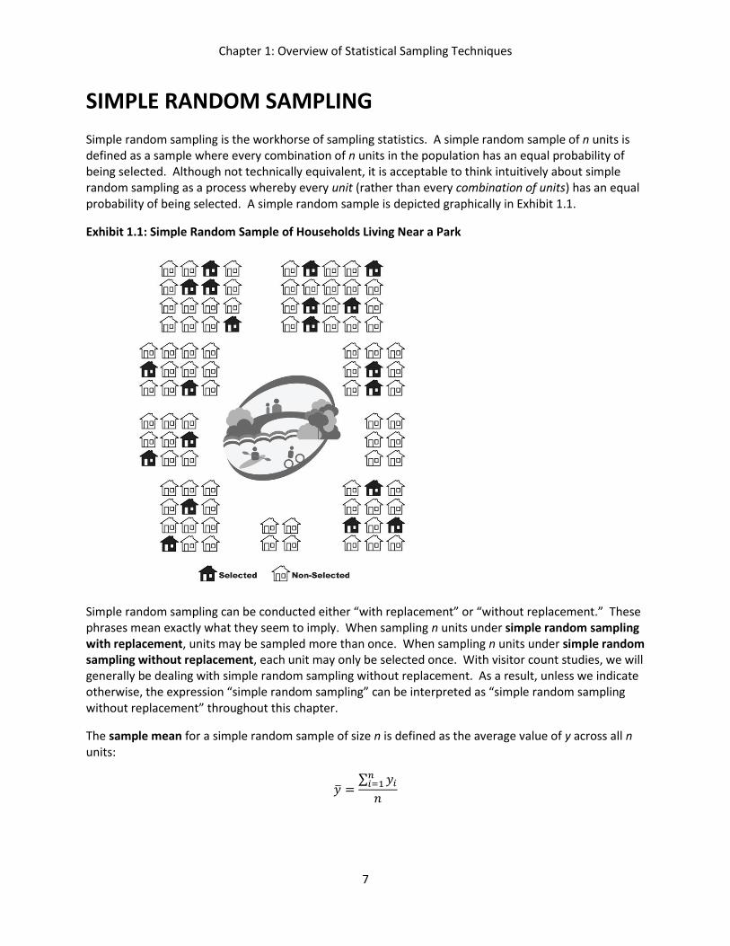
Simple random sampling is the workhorse of sampling statistics. A simple random sample of n units is defined as a sample where every combination of n units in the population has an equal probability of being selected. Although not technically equivalent, it is acceptable to think intuitively about simple random sampling as a process whereby every unit (rather than every combination of units) has an equal probability of being selected. A simple random sample is depicted graphically in Exhibit 1.1.

Exhibit 1.1: Simple Random Sample of Households Living Near a Park

Simple random sampling can be conducted either “with replacement” or “without replacement.” These phrases mean exactly what they seem to imply. When sampling n units under simple random sampling with replacement, units may be sampled more than once. When sampling n units under simple random sampling without replacement, each unit may only be selected once. With visitor count studies, we will generally be dealing with simple random sampling without replacement. As a result, unless we indicate otherwise, the expression “simple random sampling” can be interpreted as “simple random sampling without replacement” throughout this chapter.

The sample mean for a simple random sample of size n is defined as the average value of y across all n units:

�̅� =∑ 𝑦𝑖

𝑛𝑖=1

𝑛


8

while the sample variance is defined in a manner similar to the population variance: 5

𝑠2 =∑ (𝑦𝑖 − �̅�)2𝑛

𝑖=1

𝑛 − 1

As with the population variance, the sample variance can be interpreted (approximately) as the average squared deviation from the mean. The only difference is that the sample variance calculates this average for the units selected into the sample rather than for the entire population.

Recall that our goal in sampling is to obtain estimates for population parameters. With simple random sampling, the sample mean, or �̅�, provides an unbiased estimate of the population mean, or �̅�. However, although the sample mean correctly predicts the population mean on average, it will differ from the population mean for any particular sample. It is therefore important to present a measure of the variability of �̅�. The variance of �̅� is given by

𝑉(�̅�) =𝑆2

𝑛(1 −

𝑛

𝑁)

(1.1)

The interpretation of equation 1.1 is fairly straightforward when it is split into two parts. The first part

of the equation, 𝑆2

𝑛⁄ , is the variance of �̅� for a random sample that is drawn from an infinite population.6 As one would expect, the variance of �̅� increases with the population variance S2: if the units within the population are highly variable, then different random samples will provide estimates of the mean that are also highly variable.

The variance of �̅� decreases as the sample size (n) increases. This also conforms with our intuition: a larger sample size provides additional information about the population, allowing us to estimate population parameters with greater precision. Below, the variance of �̅� is plotted against sample size, holding S2 constant at one and assuming a large population. Initially the variance declines steeply as the sample size increases. However, as the sample size gets larger and larger, the marginal benefit of adding additional sample declines until it eventually approaches zero (Exhibit 1.2).

5 Note that lowercase letters are used to represent statistics calculated from the sample, while uppercase letters are used to represent population parameters. 6 It is also the variance of �̅� when sampling is conducted with replacement.


9

The second part of equation 1.1, (1 −𝑛

𝑁), is called the finite population correction (fpc) (Cochran 1977,

pg. 24). This correction factor, which always lies between zero and one (since n can’t be greater than N), scales the variance downwards to adjust for fact that we typically draw our samples without replacement from finite, rather than infinite, populations. Intuitively, if our sample represents a larger

fraction of the population (i.e., 𝑛

𝑁 is large), we have more information about the population and can

estimate the population mean with greater precision. In the extreme case, if we sample every unit in the population, n = N, the fpc is zero, and the variance of �̅� is also zero (we know the population mean exactly). Conversely, when the population is extremely large relative to the sample size, as is the case with most general population surveys, the fpc is close to one and can be ignored.

Note that in nearly all sampling contexts, we do not know the population variance (S2), so we cannot actually calculate 𝑉(�̅�). The solution is to estimate the population variance with the sample variance (i.e., replace S2 with s2) to obtain the following estimate of 𝑉(�̅�):

�̂�(�̅�) =𝑠2

𝑛(1 −

𝑛

𝑁)

As the measurement units for the estimated variance are squared, researchers typically report the square root of the estimated variance, or the standard error, for ease of interpretation:

𝑆𝐸(�̅�) = √𝑠2

𝑛(1 −

𝑛

𝑁)

The standard error for an estimate will have the same units as the original measurements.

With visitation studies, we are often more interested in estimating the population total (Y) than the population mean (�̅�) . For example, we might draw a simple random sample of days in April, count total visitors on each selected day, then extrapolate from the sampled days to estimate the total number of

0

0.05

0.1

0 50 100 150 200 250 300 350

Var

ian

ce o

f Sa

mp

le M

ean

Sample Size (n)

Exhibit 1.2: Variance of Sample Mean versus Sample Size

Note: assumes S2 = 1 and N = 10,000


10

April visitors. Under simple random sampling, �̂� = 𝑁�̅� is an unbiased estimate of Y. The estimated

standard error of �̂� is given by

𝑆𝐸(�̂�) = 𝑁√𝑠2

𝑛(1 −

𝑛

𝑁)

Although the standard error is useful and is typically reported with an estimate, non-technical readers will have difficulty interpreting standard errors. As a result, researchers often report confidence intervals for their estimates. A confidence interval provides a range within which the researcher expects the true value to lie. Recall that due to sampling error, the reported estimate is almost always not equal to the population parameter; that is, the estimate is almost always incorrect when interpreted literally. For example, when we use a general population survey to estimate that the average American has visited 4.8 national parks within the last ten years, this number is likely to be wrong. The true number may instead be 4.1 or 5.3. Confidence intervals circumvent this problem by presenting the estimate as a range rather than a single value. For example, one might present a range of 3.8 – 5.8 trips rather than using the point estimate of 4.8 trips.

Suppose we wish to estimate the value of a particular population parameter, 𝜃, and let 𝜃 represent our estimate of that parameter. An X% confidence interval for 𝜃 is an interval which, if calculated for repeated samples, would be expected to include the true parameter X% of the time. This definition, although correct, is rather convoluted. The vast majority of non-technical readers (and many technical readers) will have a different interpretation: they will assume that there is an X% chance that the true parameter lies within the X% confidence interval. Although there is a subtle difference between these two interpretations, it is likely harmless for most readers to ignore it. Interested readers can consult Lohr (1999, pp. 35-36).

The X% confidence interval for 𝜃 is calculated as

[𝐿𝑜𝑤𝑒𝑟 𝐵𝑜𝑢𝑛𝑑, 𝑈𝑝𝑝𝑒𝑟 𝐵𝑜𝑢𝑛𝑑] = [ 𝜃 − 𝑧𝑆𝐸(𝜃), 𝜃 + 𝑧𝑆𝐸(𝜃)]

The factor z is used to scale the size of the interval based on the level of confidence desired: for a 99% confidence interval, z = 2.58, for a 95% confidence interval, z = 1.96, and for a 90% confidence interval, z = 1.65. A 95% confidence interval is fairly typical. These confidence interval calculations rely on a normal approximation that is likely to be reasonable if the sample size is large and the population itself is not unusually skewed. For small sample sizes and skewed populations, the researcher should consider consulting a statistician or applying model-based methods to establish confidence intervals.7

Under simple random sampling, the 95% confidence interval for �̅� is given by

⌊�̅� − 1.96 ∗ 𝑆𝐸(�̅�), �̅� + 1.96 ∗ 𝑆𝐸(�̅�) ⌋

or

7 Often survey researchers present a “margin of error” rather than a standard error or confidence interval. The margin of error is typically equal to the half-width of a 95% confidence interval. For example, an estimate presented as “83%, +/-2%” would be equivalent to a 95% confidence interval of [81%, 85%].


11

⌊�̅� − 1.96√𝑠2

𝑛(1 −

𝑛

𝑁) , �̅� + 1.96√

𝑠2

𝑛(1 −

𝑛

𝑁) ⌋

Example 1.3: Simple Random Sampling

Suppose we would like to estimate the total number of visitors launching boats from a small launch site at Lake Roosevelt National Recreation Area during the summer months (June, July, and August). There are 92 days in the three-month period. We draw a simple random sample of 15 days, and we count visitors launching boats on all 15 days. The number of visitors observed launching boats on the sampled days is as follows:

Day No. Visitors

1 5 2 11 3 8 4 7 5 10 6 4 7 5 8 8 9 12

10 13 11 14

Simple Random Sampling: Summary of Estimators

Estimator Standard Error

Mean �̅� =

∑ 𝑦𝑖𝑛𝑖=1

𝑛

𝑆𝐸(�̅�) = √

𝑠2

𝑛(1 −

𝑛

𝑁)

where:

𝑠2 =∑ (𝑦𝑖 − �̅�)2𝑛

𝑖=1

𝑛 − 1

Total �̂� = 𝑁�̅� 𝑆𝐸(�̂�) = 𝑁 𝑥 𝑆𝐸(�̅�)


12

Day No. Visitors

12 12 13 3 14 7 15 6

The sample average is �̅� =125

15= 8.33, and the sample variance is 𝑠2 =

169.3

15−1 = 12.1. As a result, the

total estimated visitors is �̂� = 𝑁�̅� = 92 ∗ 8.33 = 766.4 with standard error equal to

𝑆𝐸(�̂�) = 𝑁√𝑠2

𝑛(1 −

𝑛

𝑁)

= 92√12.1

15(1 −

15

92)

= 75.6

Assuming normality, a 95% confidence interval can be calculated as:

⌊�̂� − 1.96 ∗ 𝑆𝐸(�̂�), �̂� + 1.96 ∗ 𝑆𝐸(�̂�) ⌋

or ⌊766.4 − 1.96 ∗ 75.6, 766.4 + 1.96 ∗ 75.6 ⌋

or

⌊618, 915 ⌋

Thus, we estimate that 766 visitors launched boats during the summer months, with a 95% confidence interval of [618, 915]. A more precise estimate (with a narrower confidence interval) could have been obtained by conducting visitor counts on a larger number of days.


13

STRATIFIED RANDOM SAMPLING

While simple random sampling has tremendous intuitive appeal, in some situations it simply does not make sense. For example, suppose we were interested in estimating annual visitation at North Beach, which is within Padre Island National Seashore, using comprehensive on-site visitor counts at all entrances to the beach. Because these on-site counts are expensive, we can’t count every single day, but our budget is sufficient to conduct visitor counts on a sample of 60 days. Under this scenario, it is difficult to imagine why it would ever make sense to use simple random sampling to select a sample of days. A simple random sample might yield 35 winter days, 12 spring days, 6 summer days, and 7 fall days. Or it might yield 0 winter days, 0 spring days, 60 summer days, and 0 fall days. These types of undesirable samples can be avoided by dividing the year into seasons, then drawing a simple random sample of days from each season.

This type of sampling, where we divide the entire population into mutually exclusive groups, then draw a simple random sample from each group, is called stratified random sampling (Exhibit 1.3). The groups are referred to as “strata.” The term “strata” has the same origin as the geological term that describes layers of sedimentary rock. Within each stratum, the rock types are similar. Across strata, they differ.

Similarly, the days in the above example are assumed to be relatively similar within a season, but to differ across seasons. In stratified random sampling, the sample within each stratum is used to characterize that stratum (e.g., average visitation for a season), then the strata results are combined to characterize the overall population (e.g., average visitation for the entire year).8

8 As a concept, stratified random sampling has been around for millennia. Plutarch (Life of Antony, c. 39) describes Antony’s application of stratified random sampling in punishing Roman soldiers after a defeat: “Antony was furious and employed the punishment known as 'decimation' on those who had lost their nerve. What he did was divide the whole lot of them into groups of ten, and then he killed one from each group, who was chosen by lot.”

Sedimentary layers, or “strata”


14

Exhibit 1.3: Stratified Random Sample of Households Living Near a Park

Households are grouped by neighborhoods, which are the strata, and a simple random sample

of households is selected from each neighborhood.

Stratified random sampling can only be implemented if (1) the entire population can be divided into mutually exclusive strata and (2) the total number of units in the population that belong to each stratum is known. If these conditions hold, then stratified random sampling can be extremely useful:

Improved Precision: If the strata are relatively homogeneous with respect to the characteristics we are measuring, stratified random sampling will typically produce estimates with lower standard errors than simple random sampling. The improvement in precision is largest when the differences among units within each stratum are small and the differences across strata are large.9 For example, stratified sampling would likely improve precision in estimating the average height of students in an elementary school, as height differences within grades are likely to be small relative to height differences across grades.

Stratum-Specific Estimates: In many cases, we would like to have estimates for subsets of the population in addition to an overall estimate. Stratified random sampling can guarantee that these stratum-specific estimates will be available. For example, in addition to the total number of annual trips to North Beach, we might be interested in estimating trips by season. When conducting an on-site count study on randomly selected days, stratifying by season

9 Note that in the extreme case, where all units are identical within strata, a stratified random sample could determine the population mean exactly by drawing only one unit from each stratum.

Strata


15

can guarantee that we will be able to estimate seasonal totals (by guaranteeing that we will select at least one day from each season), while simple random sampling cannot.

Lower Administrative Costs: There are many situations where stratification simplifies the administration of a study, thus potentially lowering costs. For example, suppose that we need to randomly select trailheads along the Appalachian Trail for a season-long count study designed to estimate the number of day hikers using the trail. It would be inefficient to draw a simple random sample of trailheads, as the selected trailheads on any given day could be anywhere along the 2,168-mile trail. Unusual samples could lead to extremely high travel costs for field personnel. It would be preferable to divide the trail into sections and sample trailheads within each section. Under this design, field staff could be hired to cover only the section of the trail that is closest to their home.

The reason stratified random sampling can improve precision is because we are adding information to the sampling problem, just as increasing the sample size adds information. Rather than approaching the problem with absolutely no knowledge of the population (other than its total size), we are exploiting knowledge about how the population should be organized before we begin sampling. It is this extra information that allows us to develop estimates that are more precise than under simple random sampling.

The mathematical notation used to describe stratified random sampling is a bit cumbersome, but easily understood with sufficient attention to detail. The key is to remember that we are simply applying simple random sampling to individual strata, then combining the stratum-specific results to obtain estimates for the population. When we combine results from individual strata, we need to take the size of each stratum into account. For example, in combining average daily visits by month to estimate average daily visits for the year, we would need to account for the fact that August has 31 days while February only has 28.

Let h be a stratum-specific subscript so that 𝑛ℎ represents the sample size in stratum h, 𝑁ℎ represents

the population size for stratum h, �̅�ℎ represents the sample mean for stratum h, and 𝑠ℎ2 represents the

sample variance for stratum h. Also, let H represent the total number of strata and let N represent the

overall population size, or 𝑁 = ∑ 𝑁ℎ𝐻ℎ=1 .

Using this notation, an unbiased estimate of the population mean is given by

�̅�𝑠𝑡𝑟 = ∑𝑁ℎ

𝑁

𝐻

ℎ=1

�̅�ℎ ,

with the estimated standard error given by

𝑆𝐸(�̅�𝑠𝑡𝑟) = √∑ (1 −𝑛ℎ

𝑁ℎ) (

𝑁ℎ

𝑁)

2 𝑠ℎ2

𝑛ℎ

𝐻

ℎ=1

.

Note that 𝑁ℎ

𝑁 is the fraction of the population that is within stratum h, so �̅�𝑠𝑡𝑟 is really just a weighted

average of the stratum-specific sample means, where the weight for each stratum is the proportion of the overall population that it represents. This makes intuitive sense. For example, suppose we conducted a phone survey of New England residents to estimate the average number of lifetime trips


16

taken to Acadia National Park. If we stratified by state and completed 100 interviews in each state, we would want to weight the state means by the relative population of each state when calculating the overall average for New England. Massachusetts, which has a population of 6.6 million, would have a weight that is approximately 11 times larger than Vermont, which has a population of 0.6 million.

It is also important to note that the sample variance (𝑠2) is undefined with a sample size of one. As a result, if a standard error for the population estimate is desired (and it usually is), it is important to ensure that at least two units from each stratum are sampled.

An unbiased estimate of the population total under stratified random sampling is

�̂�𝑠𝑡𝑟 = ∑ 𝑁ℎ

𝐻

ℎ=1

�̅�ℎ ,

with estimated standard error given by

𝑆𝐸(�̂�𝑠𝑡𝑟) = √∑ (1 −𝑛ℎ

𝑁ℎ) 𝑁ℎ

2𝑠ℎ

2

𝑛ℎ

𝐻

ℎ=1

.

If the sample sizes within each statum are large (i.e., > 30), then an approximate confidence interval is

�̅�𝑠𝑡𝑟 ± 𝑧𝑆𝐸(�̅�𝑠𝑡𝑟),

When sample sizes within strata are small, many survey researchers use a t distribution (rather than a z distribution) with n-H degrees of freedom (Lohr 1999, pg. 101). Alternative approaches are discussed in Cochran (1977, pg. 96).


17

Example 1.4: Stratified Random Sampling

Suppose we need to estimate the number of fishing trips taken to Shenandoah National Park last year from four nearby counties. Counties 1 and 2 border the park, while Counties 3 and 4 are nearby but do not border the park. We obtain a list of licensed anglers, and we sort the list by county. We find that County 1 has 7,000 licensed anglers, County 2 has 12,000, County 3 has 14,000, and County 4 has 8,000. Because anglers living closer to the park are more likely to fish there, we choose to sample 1 in 50 anglers from counties 1 and 2, and 1 in 100 anglers from counties 3 and 4, leading to sample sizes of 𝑛1 = 140, 𝑛2 = 240, 𝑛3 = 140, and 𝑛4 = 80.

We draw a simple random sample of anglers from each of the four counties, phone each selected angler, and determine the number of fishing trips that he or she took to Shenandoah last year.10 The resulting sample means are as follows: �̅�1 = 2.4, �̅�2 = 3.8, �̅�3 = 0.7, and �̅�4 = 1.2, while the sample

variances are 𝑠12 = 4.7, 𝑠2

2 = 9.7, 𝑠32 = 1.3, and 𝑠4

2 = 2.1.

Total estimated fishing trips are calculated as:

�̂�𝑠𝑡𝑟 = ∑ 𝑁ℎ

𝐻

ℎ=1

�̅�ℎ

= (7,000)(2.4) + (12,000)(3.8) + (14,000)(0.7) + (8,000)(1.2)

10 For simplicity, we assume 100% response and perfect recall.

Stratified Random Sampling: Summary of Estimators


Mean �̅�𝑠𝑡𝑟 = ∑

𝑁ℎ

𝑁

𝐻

ℎ=1

�̅�ℎ

where:

�̅�ℎ= sample mean for stratum h

Nh= total number of units in stratum h

𝑆𝐸(�̅�𝑠𝑡𝑟) = √∑ (1 −𝑛ℎ

𝑁ℎ) (

𝑁ℎ

𝑁)

2 𝑠ℎ2

𝑛ℎ

𝐻

ℎ=1

where:

𝑠ℎ2= sample variance for stratum h

nh = number of units sampled from stratum h

Total �̂�𝑠𝑡𝑟 = 𝑁�̅�𝑠𝑡𝑟 𝑆𝐸(�̂�𝑠𝑡𝑟) = 𝑁 𝑥 𝑆𝐸(�̅�𝑠𝑡𝑟)


18

= 81,800 trips

The calculation of the standard error for this total is illustrated in the following table:

h 𝑛ℎ 𝑁ℎ 𝑠ℎ2

𝑛ℎ

𝑁ℎ 𝑁ℎ

2 𝑠ℎ

2

𝑛ℎ (1 −

𝑛ℎ

𝑁ℎ) 𝑁ℎ

2𝑠ℎ

2

𝑛ℎ

1 140 7,000 4.7 0.02 49,000,000 0.034 1,632,680 2 240 12,000 9.7 0.02 144,000,000 0.040 5,644,800 3 140 14,000 1.3 0.01 196,000,000 0.009 1,746,360 4 80 8,000 2.1 0.01 64,000,000 0.026 1,647,360

Total: 10,671,200

SE(�̂�𝑠𝑡𝑟) = √10,671,200 = 3,267

Thus, the overall estimate of fishing trips to Shenandoah from the four counties is 81,800, with a 95% confidence interval of

⌊�̂�𝑠𝑡𝑟 − 1.96 ∗ 𝑆𝐸(�̂�𝑠𝑡𝑟), �̂�𝑠𝑡𝑟 + 1.96 ∗ 𝑆𝐸(�̂�𝑠𝑡𝑟) ⌋

or

⌊75,397, 88,203⌋

While stratified random sampling can be useful, it does come at a cost. First, the analysis methods are more complex than under simple random sampling, thus increasing the possibility of error and misinterpretation. For example, if another researcher inherits a survey dataset for analysis, that person will often default to assuming that the data were gathered using simple random sampling, thus leading to potentially biased estimates and/or incorrect standard errors.

Second, stratified random sampling requires more thought prior to drawing the sample. Specifically, the researcher must decide (1) how to define the strata and (2) how to allocate the sample across strata.

Defining Strata

Defining strata involves two separate decisions: (1) deciding on the total number of strata (H) and (2) deciding how to subdivide the population into these H groups. Unfortunately, there is no step-by-step process for making these decisions that will apply in all sampling contexts.11 However, there are a few general guidelines to keep in mind.

11 Cochran (1977, pp. 127-134) provides additional technical detail and discussion of research results related to these topics, but there are few general conclusions that can be drawn. If the consequences of incorrectly specifying the strata could potentially be severe (e.g., situations where data collection costs are extremely high), we recommend working with a sampling statistician to maximize the efficiency of the sampling.


19

1. When an estimate is required for a specific sub-population, that sub-population must be an individual stratum. For example, in a survey of U.S. residents designed to estimate national park visitation by state, one would want to stratify by state to ensure that each state has a sufficient number of respondents.

2. Differences between strata should be as large as possible and differences within strata should be as small as possible. Stratification provides the most improvement in precision when there are large differences between the strata, but variability within the strata is relatively small. For example, in selecting days for an on-site visitor count study, one may want to consider stratifying by season if the variation in daily visitation across seasons is large relative to the within-season variation.12

3. When faced with two possible choices for stratification, it is often preferable to select the design that is simpler and more intuitive. For example, having fewer strata is often preferable, with between two and five being sufficient in many contexts. Simple stratification schemes reduce the possibility of error during implementation and analysis, and they frequently lead to greater acceptance of the study results by decision-makers. If decision-makers can’t understand how a complex sample was drawn, there is a greater likelihood that they will view the results – however sound they may be – with skepticism.

Despite the absence of clear guidance with respect to defining strata, one should be reassured by the fact that while some stratification schemes will provide more precision than others, there is no stratification that would be considered indisputably “wrong.” Regardless of the stratification, one can always develop unbiased estimates of population parameters and calculate standard errors under stratified random sampling.

Allocating the Sample Across Strata

The simplest approach to allocating the total sample across individual strata is to use proportional allocation, which involves allocating the sample in direct proportion to stratum size.13 Under proportional allocation, the sample size for stratum h is given by:

𝑛ℎ = (𝑁ℎ

𝑁) 𝑛

With a general population survey of U.S. residents stratified by state, a sample size of 1,000 would involve sampling 121 California residents under proportional allocation, because 12.1% of U.S. residents live in California:

121 = (38 𝑚𝑖𝑙𝑙𝑖𝑜𝑛

314 𝑚𝑖𝑙𝑙𝑖𝑜𝑛) 1,000

Proportional allocation is often the best approach for allocating the sample across strata when there is little information about the potential variance of y within strata and when the cost of sampling is relatively constant across strata. The beauty of proportional allocation is that the sample mean is equal

12 In these types of studies, it is also common to stratify by type of day (e.g., weekend versus weekday). 13 This is analogous to the proportional representation that exists in the U.S. House of Representatives, where the sample size (or delegation) from each state is proportional to the state’s population.


20

to the stratified mean, or �̅�𝑠𝑡𝑟. That is, completely ignoring the stratification and calculating the sample mean in the standard way (by summing the values of y and dividing by n) provides the same result as calculating the stratified mean using the formula above. This simplifies interpretation and analysis, and it reduces the likelihood that subsequent researchers inheriting the dataset will misinterpret the data.

When the variance of y is expected to be larger in some strata than in others, then the sampling will be more efficient if a larger share of the overall sample is allocated to the high-variance strata. High-variance strata are somewhat like the problem children in a large family: they demand more of our attention because their behavior is unpredictable. Suppose, for example, we were selecting days for a summer/fall count study at a beach in northern California. In the summer, the weather is relatively cool, foggy, and predictable. In the fall, it is generally somewhat cool but occasionally there are spectacular beach days. Under this scenario, we would want to allocate more sampling days to the fall than to summer, as visitation in the fall would have greater variability.14

When the cost of sampling is constant across strata, the most efficient allocation approach is Neyman allocation (Neyman 1934).15 Under Neyman allocation, the sample size for stratum h is proportional to the size of the stratum (𝑁ℎ) times the stratum standard deviation (𝑆ℎ):

𝑛ℎ = (𝑁ℎ𝑆ℎ

∑ 𝑁ℎ𝑆ℎ𝐻ℎ=1

) 𝑛

This makes sense intuitively: we allocate more of the sample to strata that (1) are difficult to characterize due to their variability and (2) have an outsized influence on the population mean/total because they constitute a large share of the overall population.

The conundrum with Neyman allocation is that it requires information about stratum variances, yet we typically can’t estimate variances until the study is actually implemented. As a result, the most efficient sampling approach can’t be established until after we’ve finished sampling! While this may seem like a hopeless situation, it is sometimes possible to gain enough information about variances that would allow us to at least approximate Neyman allocation. For example, preliminary information about variances might be obtained from a small-scale pilot effort conducted prior to the main study (e.g., the first phase of a multi-phased study), a similar study conducted at a nearby location, or from a similar study conducted in a prior year.

Given the scarcity of information that can be used to approximate variances, we have often defaulted to a simpler approach. Specifically, we begin with proportional allocation, then adjust these initial sample sizes to allocate more of the sample to strata where we expect higher variances. Typically, strata that have larger y values (e.g.., weekends/holidays in studies designed to obtain daily counts), will have larger variances, so we oversample these strata. While perhaps not perfectly efficient, it is important to

14 Note that this assumes that the overall goal is to minimize the variance of the annual trip estimate. However, due to consistently high visitation in the summer, it is possible that obtaining a highly accurate summer-specific estimate may be more important for policy (or NRDA) purposes, which would lead one to allocate a greater share of the sample to the summer stratum. 15 When the cost of sampling differs across strata, the sampling approach can be further modified to take stratum-specific costs into account. The most efficient approach is called “optimal allocation” and involves allocating the

sample in proportion to 𝑁ℎ𝑆ℎ

√𝑐ℎ, where 𝑐ℎ is the unit cost of an observation in stratum h.


21

keep in mind that our estimates will be unbiased regardless of the allocation of the sample across strata; it’s just that a more efficient allocation will produce smaller standard errors.


22

Cluster Sampling

Suppose we were planning to conduct an in-person survey of Washington D.C. households to estimate annual visits to the National Mall. A random sample of households in the city would likely be very costly for conducting interviews, as selected households would potentially be widely dispersed throughout the city. It would be time consuming for interviewers to travel to all of the selected households. An alternative would be to group households into clusters based on location (e.g., neighborhoods or blocks), randomly select a subset of these clusters, then randomly select households within each cluster (Exhibit 1.4). This approach would result in sampled households that are closer together, thus reducing travel costs for interviewers.

Exhibit 1.4: Two-Stage Cluster Sample of Households Living Near a Park

Households are grouped by neighborhood, then a simple random sample of three

neighborhoods are selected. Within each of the selected neighborhoods,

a simple random sample of households is selected.

Clusters


23

Consider another example where the sampling unit is a recreational trip rather than a household. Suppose we would like to estimate mean trip length at a park by randomly selecting survey days, then interviewing a sample of visitors leaving the park on the selected days. In this example, trips are naturally grouped in clusters: each day is a cluster of trips. Thus, our sampling approach involves randomly selecting clusters, then selecting a subset of trips within each selected cluster.

These examples describe two-stage cluster sampling (Exhibit 1.5). The first stage involves selecting one or more clusters, or groups, of sampling units. The second stage involves selecting sampling units within each selected cluster.16 Cluster sampling is similar to stratified random sampling in that both require that the entire population be divided into mutually exclusive groups prior to drawing the sample. However, with stratified sampling, sampling units are selected within every group. With cluster sampling, on the other hand, some groups will have units selected while others will not. Thus, cluster sampling concentrates (or “clusters”) the sample within a subset of the groups.

Exhibit 1.5: Two-Stage Cluster Sampling

Stage 1:

Stage 2:

Cluster sampling typically provides less precision than simple random sampling or stratified random sampling when the sample size is held constant. This is due to the fact that units within a cluster are often similar to one another. As a result, concentrating the sample within a small number of clusters provides less information about the research problem: an additional unit from a cluster provides little new information if it is similar to all of the other units in that cluster. Consider, for example, the problem of estimating average household income within a metropolitan area by drawing a sample of households and conducting a survey. As households living within the same neighborhood tend to be broadly similar with regard to socioeconomic status, spreading the sample across many different neighborhoods (through simple random sampling or stratified random sampling) would clearly provide more information than concentrating the sample within only a few neighborhoods (through cluster sampling).

Under cluster sampling, precision will be greatest when variability within clusters is large and variability across the clusters is small.17 In other words, when the units within the clusters don’t really seem to

16 Sampling texts typically present many more varieties of cluster sampling than are described here. Specifically, these texts will describe cluster sampling where all units within each cluster (rather than just a subset of units) are sampled and examined. They also describe situations where the clusters each have the same number of sampling units and situations where the total number of sampling units (N) is known. 17 Note that the opposite is true with stratified random sampling, where it is preferable to have more variability across strata and less variability within strata.

Randomly select

clusters of units

Randomly select

units from each

selected cluster


24

naturally belong together, precision will be higher. Ideally, one would have clusters that are very diverse, so that each cluster can be thought of as a “mini population.” In the extreme case, if there were no differences between clusters, then a cluster sample would be equivalent to a simple random sample, because the cluster membership of the sampled units would be irrelevant.

In order to describe the relevant formulas for cluster sampling, some new notation will be required:

N = total number of clusters

n = number of randomly selected clusters

Mi = total number of sampling units within the ith sampled cluster

mi = number of randomly selected units within the ith sampled cluster

�̅�𝑖 = sample mean within the ith cluster

𝑠𝑖2 = sample variance within the ith cluster

The population mean can then be estimated using a “ratio estimator":

�̅�𝑐𝑙𝑢 = ∑ 𝑀𝑖�̅�𝑖

𝑛𝑖=1

∑ 𝑀𝑖𝑛𝑖=1

While this expression may look unusual at first, it is really just a weighted average of the sample means (�̅�𝑖) for the selected clusters, where the weights are the cluster sizes (𝑀𝑖). This is consistent with intuition: larger clusters should have a greater impact on the population mean. Note that if all of the clusters are the same size (i.e., 𝑀𝑖 is a constant) then �̅�𝑐𝑙𝑢 is simply the overall average of the sampled cluster means.

The standard error of the population mean can be estimated by (Lohr 1999, pg. 148):

𝑆𝐸(�̅�𝑐𝑙𝑢) =1

�̅�√[(1 −

𝑛

𝑁)

𝑠𝑟2

𝑛+

1

𝑛𝑁∑ 𝑀𝑖

2

𝑛

𝑖=1

(1 −𝑚𝑖

𝑀𝑖)

𝑠𝑖2

𝑚𝑖]

where �̅� is the average size of the sampled clusters and 𝑠𝑟2 is an estimate of the variation across

clusters:

𝑠𝑟2 =

∑ (𝑀𝑖�̅�𝑖 − 𝑀𝑖�̅�𝑐𝑙𝑢)2𝑛𝑖=1

𝑛 − 1

(1.2)

Note that equation 1.2 is simply the average squared deviation of the cluster means from the population mean, where the deviations are weighted by cluster size.

An unbiased estimator of the population total is given by:

�̂�𝑐𝑙𝑢 =𝑁

𝑛∑ 𝑀𝑖𝑦�̅�

𝑛

𝑖=1

(1.3)


25

In equation 1.3, 𝑀𝑖�̅�𝑖 is just the size of cluster i times the sample mean for cluster i, which is of course a natural estimate of the total for cluster i. These estimated cluster totals are summed across all sampled

clusters, and the result is scaled up to the population by multiplying by 𝑁

𝑛, or the inverse of the fraction

of clusters in our sample.

The standard error is estimated by (Lohr, 1999, pg. 147):

𝑆𝐸(�̂�𝑐𝑙𝑢) = √𝑁2 (1 −𝑛

𝑁)

𝑠𝑌2

𝑛+

𝑁

𝑛∑ (1 −

𝑚𝑖

𝑀𝑖) 𝑀𝑖

2𝑠𝑖

2

𝑚𝑖

𝑛

𝑖=1

where we define 𝑠𝑌2 as:

𝑠𝑌2 =

∑ (𝑀𝑖�̅�𝑖 −�̂�𝑐𝑙𝑢𝑁 )

2𝑛𝑖=1

𝑛 − 1.

When designing a study involving two-stage cluster sampling, the analyst will often need to make difficult decisions about how to allocate the total sample across and within clusters. For example, if the overall sample size is fixed due to budget constraints, do we select many clusters and only a few sampling units within each selected cluster? Or do we select a few clusters but many sampling units within each selected cluster? It turns out that when the number of clusters in the population (N) is large, the former approach is almost always preferable – to select many clusters and only a few sampling units within each selected cluster. This is apparent when one examines the standard error formulas above: when N is large, the variation across clusters (𝑠𝑟

2) becomes much more important than

the variation within clusters (𝑠𝑖2).


26

Cluster Sampling: Summary of Estimators


Mean �̅�𝑐𝑙𝑢 =

∑ 𝑀𝑖�̅�𝑖𝑛𝑖=1


where:

�̅�𝑖 = sample mean of the ith cluster 𝑀𝑖= total number of units in the ith cluster n = number of randomly selected clusters

𝑆𝐸(�̅�𝑐𝑙𝑢) =1

�̅�√[(1 −

𝑛

𝑁)

𝑠𝑟2

𝑛+

1


2

𝑛

𝑖=1

(1 −𝑚𝑖

𝑀𝑖

)𝑠𝑖

2

𝑚𝑖

]

where:

�̅� = average number of units in the sampled clusters N = total number of clusters 𝑚𝑖= number of units selected from the ith cluster

𝑠𝑟2 =

∑ (𝑀𝑖�̅�𝑖 − 𝑀𝑖�̅�𝑐𝑙𝑢)2𝑛𝑖=1

𝑛 − 1

𝑠𝑖2 = sample variance within the ith cluster

Total �̂�𝑐𝑙𝑢 =

𝑁


𝑛

𝑖=1

𝑆𝐸(�̂�𝑐𝑙𝑢) = √𝑁2 (1 −𝑛

𝑁)

𝑠𝑌2

𝑛+

𝑁

𝑛∑ (1 −

𝑚𝑖

𝑀𝑖

) 𝑀𝑖2

𝑠𝑖2

𝑚𝑖

𝑛

𝑖=1

where:

𝑠𝑌2 =

∑ (𝑀𝑖�̅�𝑖 −�̂�𝑐𝑙𝑢𝑁 )

2𝑛𝑖=1

𝑛 − 1.


27

Example 1.5: Cluster Sampling

Suppose we would like to estimate the average duration of a visit to Arches National Park in August. We randomly select five days and we conduct exit interviews at the main entrance with every fifth visitor on the selected days.18

We obtain the following data from the five days of sampling:

Day

i

Number of

Visitors Observed

𝑀𝑖

Number of Completed Interviews

𝑚𝑖

Sample Average Trip Length

(hours)

�̅�𝑖

Sample Variance of Trip Length

𝑠𝑖2

Intermediate Term in SE Calculation

𝑀𝑖2 (1 −

𝑚𝑖

𝑀𝑖)

𝑠𝑖2

𝑚𝑖

1 400 80 4.5 9.1 14,560 2 600 120 3.2 8.7 20,880 3 225 45 5.6 5.8 5,220 4 1,600 320 2.3 6.9 44,160 5 200 40 6.0 7.0 14,560

The average visit duration is estimated as

�̅�𝑐𝑙𝑢 = ∑ 𝑀𝑖�̅�𝑖

𝑛𝑖=1


=(400)(4.5)+(600)(3.2)+(225)(5.6)+(1,600)(2.3)+(200)(6.0)

(400+600+225+1600+200)

= 3.3 hours

The between-cluster variance is estimated as:

𝑠𝑟2 =

∑ (𝑀𝑖�̅�𝑖 − 𝑀𝑖�̅�𝑐𝑙𝑢)2𝑛𝑖=1

𝑛 − 1

=(400(4.5 − 3.3) + 600(3.2 − 3.3) + 225(5.6 − 3.3) + 1,600(2.3 − 3.3) + 200(6.0 − 3.3))

4

= 795,520

Finally, the standard error of the estimated mean is calculated as:

18 Although this is a systematic sample of trips, we will treat it as a simple random sample in this example.


28

𝑆𝐸(�̅�𝑐𝑙𝑢) =1

�̅�√[(1 −

𝑛

𝑁)

𝑠𝑟2

𝑛+

1


2

𝑛

𝑖=1

(1 −𝑚𝑖

𝑀𝑖)

𝑠𝑖2

𝑚𝑖]

=1

605√[(1 −

5

31)

795,520

5+

1

5 ∗ 31(14,560 + 20,880 + 5,220 + 44,160 + 14,560))]

= 0.61 ℎ𝑜𝑢𝑟𝑠

Thus, the estimated mean duration of a trip is 3.3 hours , with a 95% confidence interval (assuming normality) of

⌊�̅�𝑐𝑙𝑢 − 1.96 ∗ 𝑆𝐸(�̅�𝑐𝑙𝑢), �̅�𝑐𝑙𝑢 + 1.96 ∗ 𝑆𝐸(�̅�𝑐𝑙𝑢) ⌋

or

⌊2.1, 4.5⌋


29

Systematic Sampling

There are times when it can be extremely difficult to draw a simple random sample. Suppose, for example, that we wanted to determine the average length of trips taken to the Statue of Liberty on a particular day. We could assign every visitor a unique ID upon entering the park, then draw a simple random sample of these IDs at the end of the day. But at the end of the day, all of the visitors would be gone, so it would be impossible to conduct any interviews! Alternatively, we could collect phone numbers from visitors as they enter the park, randomly draw a simple random sample of these phone numbers at the end of the day, and call each selected visitor. However, this would require stopping all visitors and requesting phone numbers (not just the sampled visitors), which is a burdensome task. Furthermore, many visitors would refuse to provide a phone number, provide an invalid number, or simply refuse to answer the phone when called.

As an alternative, on-site intercept interviews are typically conducted using systematic sampling. Under systematic sampling, a sampling interval (k) is selected, and every kth visitor leaving the facility or park is intercepted and interviewed. This is equivalent to having a complete list of visits, sorting the list by departure time, then selecting every kth visit from the sorted list. In order to ensure that every visitor has the same probability of selection, the starting point (between 1 and k) must be randomly selected. Continuing the example above, suppose we decided to interview every 4th visitor leaving the Statue of Liberty. We randomly select a number between 1 and 4, and we end up selecting the number 3. We would then sample visitor numbers 3, 7, 11, 15, etc:

A second example is depicted in Exhibit 1.6, which shows a systematic random sample of houses near a park. Here, the houses are ordered from left to right, then from top to bottom. Every 5th house is selected, with the randomly selected starting point being house number two. Note that one of the neighborhoods has none of its houses selected and another (on the lower right) has half of its houses selected.

Systematic sampling offers several advantages over simple random sampling:

When it is difficult to convert the population to a computerized list, systematic sampling can be much simpler to implement than simple random sampling. This is frequently the case when sampling is conducted in the field. For example, consider the problem of sampling occupied campsites at a large campground. While it would be possible to enter the site numbers associated with all occupied campsites into a spreadsheet, then draw a simple random sample, this process may be cumbersome for field personnel to implement. It is much simpler to have field personnel walk through the campground in a pre-determined order (i.e., by campsite number), conducting interviews at every kth occupied campsite.

Systematic sampling can protect against the possibility of an unusual sample that would not be representative of the population. In the campsite example, simple random sampling could potentially result in a sample of campsites that are all located in a single area of the campground. For example, the entire sample could consist of campsites that are close to a

1 2 3 4 5 6 7 8 9 10 11 12 13 14 15 16


30

nearby lake, thus potentially leading to an overestimate of the total number of beach trips. A systematic sample would spread the sample throughout the campground.

Systematic sampling is actually a type of cluster sampling, but only one cluster is selected. For example, suppose we are selecting a systematic random sample of individuals from the following list, using a sampling interval of three:

It is easy to see that this really boils down to selecting one out of three possible clusters of individuals, depending on the randomly selected starting point:

Start = 1 Start = 2 Start = 3

The primary disadvantage of systematic sampling is that the variability can be large if the underlying population exhibits a systematic pattern that coincides with the sampling interval. For example, suppose a campground were set up so that every fourth site was an “extended stay” site, and we had a sampling interval of four. In this case, our sample would contain either all extended stay sites (0.25 probability) or none (0.75 probability). Alternatively, suppose we were selecting a systematic sample of summer days for a count study. If the sampling interval were seven, we would have only one type of day in our sample (e.g., all Mondays, all Tuesdays, etc.)! It is important to be on the lookout for these types of patterns before choosing a systematic sampling approach.

An additional disadvantage arises when using systematic sampling to conduct interviews with visitors leaving a park: we cannot specify a sample size in advance. The final sample size can of course be approximated (after selecting a sampling interval) based on previous estimates of daily visitation, but visitation on the selected day may be much higher or lower than average. Thus the ultimate sample size may be larger or smaller than desired.

Systematic random samples are typically analyzed as if they were simple random samples. That is, estimates are developed using the formulas presented previously for simple random sampling. The standard errors for simple random sampling will be reasonably accurate if the population is in approximately random order prior to drawing the sample. If the population is sorted by the variable of interest, then estimates based on systematic samples will often have lower standard errors than estimates based on simple random samples: systematic sampling forces the sampled units to be “spread out” across the potential values in the population, while simple random sampling does not. Thus, applying the formula for simple random sampling will produce a standard error estimate that is conservative (i.e., too high).19

19 Unfortunately, it is not possible to calculate the correct, lower standard error. With only one “cluster” being sampled, there simply is no way to estimate the between-cluster variance.

Bruce Daphne

Matt Sam

Chris Heather

Nora Sophie

Connor Mark

Ryan Sydney

Bruce Chris Connor Daphne Heather Mark Matt Nora Ryan Sam Sophie Sydney


31

Exhibit 1.5: Systematic Random Sample of Households Living Near a Park

Every 5th household is selected, proceeding from left to right, then from top to bottom. The

starting point was randomly selected to be the second household.


32

Ratio Estimation

Stratified random sampling provided an approach to using information from outside the sample to obtain estimates with lower variance. That is, even if we didn’t know the particular value (y) for non-sampled units, we still knew to which stratum each of those units belonged. This knowledge allowed us to exploit the relationship between stratum membership and the y values for the sampled units to obtain improved estimates of population parameters. The key was that we knew about the stratum membership for both the sampled and the non-sampled units in the population.

Suppose we had access to additional information about the non-sampled units. Our intuition tells us that we might be able to exploit this information to further reduce the variance of our estimates. For example, suppose we need to estimate summer visitation at a park that has a vehicle counter installed at the main entrance. Through a field study, we obtain information about the number of visitors entering the park on a sample of days. We can estimate summer visitation by multiplying the average number of visits on the sampled days (�̅�) by the total number of days (N), but intuition tells us that we could potentially do better by exploiting information from the vehicle counter. In Exhibit 1.7, daily visits are plotted on the vertical axis, while daily vehicle counts are plotted on the horizontal axis. There is clearly a close relationship between visits and vehicles, and it appears that the vehicle counts could provide important supplemental information about visitation on the non-sampled days.

Exhibit 1.7: Visitor and Vehicle Counts on Randomly Selected Days

Ratio estimation takes advantage of this type of supplemental information. Specifically, ratio estimation uses the relationship between the variable of interest (y) and an auxiliary variable (x) that is correlated with y in order to improve our estimates of population parameters.20 In the above example, y

20 In a well-known early example of ratio estimation, the French mathematician Pierre-Simon Laplace estimated the population of France in 1802 by calculating the ratio of total population to live births within a sample of 30 parishes (Lohr 1999). Data on live births for these 30 parishes (and for the entire country) were readily available through baptism registries. The ratio from the 30 parishes was applied to the number of live births nationwide to estimate the population of the country.


33

would be daily visitation and x would be the daily vehicle count. If we know the vehicle count for the entire population of days and, based on the sampled days, we have information about the relationship between these vehicle counts and visitation, then we can implement a ratio estimation approach. Ratio estimation allows us to leverage information about the auxiliary variable when applying the sample information to the population.

Ratio estimation is most useful under the following conditions:

When it is relatively inexpensive to obtain data on the auxiliary variable. For example, obtaining daily vehicle counts using an automated car counter is much less expensive than obtaining visitor counts with on-site personnel. It is important to note, however, that in order to implement ratio estimation data on the auxiliary variable must be available for the entire population (not just for the sample).

When there is a strong relationship between the auxiliary variable and the variable of interest. Ideally, the relationship would be linear, and the best-fit line would pass through the origin. For example, the relationship between daily vehicle counts and daily visitors would likely be strong in parks where the vast majority of visitors enter in a vehicle. The relationship would typically pass through the origin (at least approximately), because there would be no visitors on days when no vehicles enter the park.

Letting X represent the population total for the auxiliary variable (e.g., number of vehicles) and letting r represent the ratio of the sample mean of y to the sample mean of x (this is the “ratio” in the term “ratio estimate”),21

𝑟 =�̅�

�̅�

the ratio estimate of the population mean is given by

�̅�𝑟𝑎𝑡𝑖𝑜 = 𝑟𝑋

𝑁.

Continuing the example from above, the ratio estimate is simply the persons per vehicle on the

randomly sampled days (�̅�

�̅�) times the average number of vehicles per day throughout the entire three-

month period.

The standard error of �̅�𝑟𝑎𝑡𝑖𝑜 is approximated by

𝑆𝐸(�̅�𝑟𝑎𝑡𝑖𝑜) = √(𝑁 − 𝑛

𝑁)

𝑠𝑟𝑎𝑡𝑖𝑜2

𝑛

where

21 If the relationship between x and y can be summarized by a straight line that passes through the origin and if the variance of 𝑦𝑖 about this line is proportional to 𝑥𝑖, then this estimate of the ratio (r) is equivalent to the estimated slope in a weighted least squares regression, with weights equal to the inverse of 𝑥𝑖 (Lohr, 1999, pg. 71).


34

𝑠𝑟𝑎𝑡𝑖𝑜2 =

∑ (𝑦𝑖 − 𝑟𝑥𝑖)2𝑛𝑖=1

𝑛 − 1

Note that the equation for 𝑠𝑟𝑎𝑡𝑖𝑜2 is analogous to the equation for 𝑠2, the sample variance under simple

random sampling. Both expressions calculate an average squared deviation from a predicted value. But under simple random sampling the predicted value is the sample mean (�̅�), while under ratio estimation, the predicted value is 𝑟𝑥𝑖.22

The ratio estimate of the population total is

�̂�𝑟𝑎𝑡𝑖𝑜 = 𝑟𝑋

with standard error approximated by:

𝑆𝐸(�̂�𝑟𝑎𝑡𝑖𝑜) = √𝑁(𝑁 − 𝑛)𝑠𝑟𝑎𝑡𝑖𝑜

2

𝑛.

Ratio estimates are biased, but the reduced standard errors typically compensates for the bias (Lohr, 1999, pg 66). The bias declines as the sample size increases, the sampling fraction increases, the variance of x decreases, and the correlation between x and y approaches one. Lohr (pp. 66-70) and Cochran (1977, pp. 160-162) provide additional discussion of bias in ratio estimation.

22 In addition, as noted by Cochran (1977, pg. 155), 𝑠𝑟𝑎𝑡𝑖𝑜

2 is actually a biased estimate of the variance of y about the best-fit line, but the bias is of order 1/n and can therefore be safely ignored in large samples.


35

Ratio Estimation: Summary of Estimators


Mean �̅�𝑟𝑎𝑡𝑖𝑜 = 𝑟

𝑋

𝑁

where:

r = ratio of sample mean for variable of interest (�̅�) to sample mean for the auxiliary variable (�̅�)

X = population total for the auxiliary variable

𝑆𝐸(�̅�𝑟𝑎𝑡𝑖𝑜) = √(𝑁 − 𝑛

𝑁)

𝑠𝑟𝑎𝑡𝑖𝑜2

𝑛

where:



𝑛 − 1

Total �̂�𝑟𝑎𝑡𝑖𝑜 = 𝑟𝑋


2

𝑛


36

Example 1.6: Ratio Estimation

We would like to estimate summer (June/July/August) visitation at a park that has a vehicle counter installed at the main entrance. We count visitors on 15 randomly selected days and obtain the following data:

i

Visitor Count

yi

Vehicle Count

xi

Overall Visitor/Vehicle

Ratio

𝑟 =�̅�

�̅�⁄

Predicted Visitors

𝑟𝑥𝑖

Squared Deviation from

Predicted Visitors

(𝑦𝑖 − 𝑟𝑥𝑖)2

1 300 550 0.67 367 4,489 2 650 875 0.67 583 4,489 3 1040 1620 0.67 1,080 1,600 4 700 990 0.67 660 1,600 5 300 610 0.67 407 11,449 6 1550 2165 0.67 1,443 11,449 7 1150 2025 0.67 1,350 40,000 8 620 630 0.67 420 40,000 9 800 1400 0.67 933 17,689 10 350 325 0.67 217 17,689 11 1300 2000 0.67 1,333 1,089 12 225 288 0.67 192 1,089 13 935 1442 0.67 961 676 14 810 1255 0.67 837 729 15 1270 1825 0.67 1,217 2,809

12,000 18,000 156,846

We are told that throughout the entire three-month period, the total vehicle count was 115,000. Thus, the ratio estimate of total visitation is given by

�̂�𝑟𝑎𝑡𝑖𝑜 = 𝑟𝑋

= 0.67(115,000)

= 77,050 𝑣𝑖𝑠𝑖𝑡𝑜𝑟𝑠

The ratio variance is estimated as:



𝑛 − 1

=156,846

15−1

= 11,203

So that the standard error of the ratio estimate of total visitation can be calculated as


37


2

𝑛

= √92(92 − 15)11,203

15

= 2,300

Note that we could also ignore the vehicle count data and simply apply the simple random sampling formulas to estimate Y. If we do this, we obtain an estimate of 72,800 visitors, which is fairly close to the ratio estimate of 77,050 vistors. However, the standard error calculated using simple random sampling formulas is 8,856, which is much larger than the standard error of the ratio estimate, or 2,300. This shows that the ratio estimate is performing as expected: it is allowing us to improve the precision of our estimate by incorporating information from supplemental data on vehicle counts.


38

Sampling Weights

When any of the above sampling methods are applied, survey practitioners often develop sampling “weights” in order to simplify statistical analyses. The sampling weight for unit i, 𝑤𝑖, is simply the inverse of the probability that the unit was selected into the sample: it indicates the number of units in the population that the observation “represents.” Letting 𝑝𝑖 represent the selection probability for unit i, the sampling weight is given by:

𝑤𝑖 =1

𝑝𝑖

The sum of the sampling weights in a dataset equals the overall population size:

∑ 𝑤𝑖 = 𝑁

𝑛

𝑖=1

Suppose, for example, that we use simple random sampling to select 5 out of 100 possible visitors for a survey. The selection probability for any individual visitor is 5/100 = 0.05, and the inverse of the selection probability is 20 = 1/(0.05). Thus, each of the 5 visitors selected into our sample would be assigned a weight of 20, and the sum of the weights across the 5 visitors in our sample would be 20+20+20+20+20 = 100, or the population size.

While simple random sampling is helpful in illustrating the construction of weights, the true usefulness of survey weights comes into play when selection probabilities are not equal. Consider the application of weights under stratified random sampling. Suppose there are two neighborhoods near a park: Neighborhood A has 200 residents and Neighborhood B has 400 residents. Neighborhood A is closer to the park than Neighborhood B, and we therefore choose to oversample Neighborhood A when conducting a survey to estimate annual trips. We select 8 residents from Neighborhood A and 4 residents from Neighborhood B and obtain the following results:23

Neighborhood Person No. Trips

A 1 4 2 9 3 3 4 2 5 10 6 1 7 0 8 8

B 1 3 2 2 3 5 4 0

23 Clearly, any real survey would have a sample size larger than 12, but a small sample is used here for convenience.


39

Using the traditional stratified random sampling formula, we would estimate total trips as

�̂�𝑠𝑡𝑟 = ∑ 𝑁ℎ

𝐻

ℎ=1

�̅�ℎ = 200 𝑥 (4 + 9 + 3 + 2 + 10 + 1 + 0 + 8)

8+ 400 𝑥

(3 + 2 + 5 + 0)

4

But note that we could also estimate total trips using sampling weights. The sampling weight for any resident of Neighborhood A is 25 = (8/200)−1 and the sampling weight for any resident of Neighborhood B is 100 = (4/400)−1. After calculating these weights, total trips can be estimated by multiplying trips by the sampling weight for each individual, then summing the result across all sampled individuals:

�̂� = ∑ 𝑤𝑖𝑦𝑖

𝑛

𝑖=1

= 25(4 + 9 + 3 + 2 + 10 + 1 + 0 + 8) + 100(3 + 2 + 5 + 0)

Note that this provides the same result as the stratified random sampling formula.

With sampling weights, one can easily see why oversampling specific strata does not lead to biased estimates of trips. When certain types of units are sampled at higher rates, they are also assigned lower weights and therefore have less influence on the final estimates. In the above example, individuals in Neighborhood A were sampled at four times the rate of individuals in Neighborhood B. As a result, the weights for individuals from Neighborhood B (100) are four times larger than the weights for individuals from Neighborhood A (25). Thus, the sampling weights exactly compensated for the higher selection probabilities in Neighborhood A. This type of compensation occurs within the standard formulas as well, but it is somewhat buried in the math and difficult to see as clearly.

40

CHAPTER 2

ON-SITE COUNTS BY FIELD PERSONNEL

While obtaining visitation estimates through on-site counts is fairly straightforward at parks that require all visitors to pay an entry fee and pass through a main entrance, it can be quite complicated at the many parks that deviate from this simplistic structure. These parks will often require random sampling of time periods and/or count locations, with a corresponding increase in analytical complexity. This chapter provides an overview of the types of methodologies available in these contexts. The primary focus is on count efforts where data are gathered entirely by humans stationed in the field. Study designs that supplement these data with information from various types of automated counters are discussed in Chapter 3, while off-site data collection approaches are discussed in Chapter 4.

The chapter begins with an overview of the statistical sampling framework for on-site count studies, as an understanding of the sampling context is crucial to evaluating study design and data analysis options. Next, we discuss the random sampling of days, which is typically the first step in all on-site count studies, regardless of the design. We then describe a variety of potential designs for studies that directly count completed trips at site entrances. The chapter concludes with a discussion of designs where visitation estimates are derived indirectly by estimating visitor hours through instantaneous counts, then dividing this visitor-hour estimate by the average length of a trip.

OVERVIEW

For the on-site count studies discussed in this chapter, it is assumed that the ultimate goal is to estimate the number of recreational trips to a site during a specific time period. A recreational trip is defined as an occasion where an individual travels from an overnight location (e.g., a home or hotel) to spend time at a site for recreational purposes, then leaves the site and returns to the overnight location. A recreational trip might last ten minutes or it might last ten days. If the individual leaves the site briefly during the trip without returning to his or her overnight location (e.g., to get something from a vehicle or to have lunch at a nearby restaurant), we treat the individual as having taken only one trip to the site.

Chapter 2: On-Site Counts by Field Personnel

41

There are two basic approaches to estimating trips through an on-site count study (Exhibit 2.1). The first, which we call departure counts, involves stationing field personnel at entrances and counting visitors as they leave the site.24 This approach is simple and intuitively appealing, as trips are counted directly. If the number of entrances is small, field personnel can be stationed at all entrances on randomly selected days. This approach is described under simple departure counts below. In order to limit extremely long work days, it is sometimes more convenient to obtain departure counts for individual shifts (i.e., AM or PM shifts) rather than entire days. A methodology that relies on these shift-specific counts is described under departure counts with sampling of shifts. Finally, when the number of entrances is large, trip estimates can be obtained by stationing field personnel at a sample of entrances. This approach is described under departure counts with sampling of a single entrance and departure counts with sampling of multiple entrances.

The second approach, which we call instantaneous counts, involves obtaining near-instantaneous counts of all visitors on site at a sample of times in order to estimate total “visitor-hours” at the site. The visitor-hour total is divided by the duration of an average visit to convert visitor-hours to visits. Instantaneous counts are frequently used at sites where entry to the site is diffuse, making departure counts difficult to implement. This is often the case, for example, at long ocean beaches paralleled by boardwalks or sidewalks.25

Regardless of the methodology used for on-site counts, the first step is to select a subset of days on which to implement the counts. We describe common approaches to sampling days below. We then discuss each of the on-site count methodologies described in Exhibit 2.1.

24 Although one can also count visitors as they enter the site, we focus on departure counts in this chapter as we find them to be preferable to entry counts in a variety of situations. For example, if visitors will be interviewed (in addition to being counted), they will be able to provide more accurate information about trip activities and the length of the trip if the interview is conducted at the end of the trip. 25 If the border of such a site can be partitioned into mutually exclusive segments that can be monitored by field personnel, it would still be possible to apply a methodology that involves directly counting visitors as they enter or leave the site. For example, a field observer could monitor a single segment of the border and count all visitors who cross that particular segment to leave the park.


42

Exhibit 2.1: Overview of Methodologies for On-Site Count Studies

Methodology Quantity Measured Sampled Unit Quantity Estimated

Simple Departure Counts Completed trips on sampled days

Days Trips

Departure Counts with Sampling of Shifts

Completed trips on sampled shifts

Days, then shifts Trips

Departure Counts with Sampling of a Single Entrance

Completed trips on sampled days at sampled entrances

Days, then entrances Trips

Departure Counts with Sampling of Multiple Entrances

Completed trips on sampled days at sampled entrances

Days, then entrances Trips

Instantaneous Counts Persons on site at a given time Trip duration

Days, then times Days, then completed trips

Visitor-hours Mean trip duration

SELECTING DAYS FOR ON-SITE COUNTS

Typically, funding is insufficient to count visitors on every day of the time period of interest. Instead, visitors are counted on a sample of days, and total visitation is estimated by extrapolating from this sample. It is common to stratify by weekend/weekday and by month when drawing a sample of days for on-site counts (see an example in Exhibit 2.2). The weekend/weekday distinction is important because at recreation sites, visitation on Saturdays and Sundays is typically much greater than visitation on weekdays.26 Recall that stratification provides precision gains when sampling units that are similar are grouped together. Thus, placing all Saturdays and Sundays in one stratum and placing all weekdays in a second stratum will typically improve precision. Furthermore, as we learned in Chapter 1, allocating a disproportionate share of the sample to high-variance strata provides precision gains. The variance is typically higher for weekend days, so one would want to sample these days at a higher rate than weekdays.

26 Holidays such as Memorial Day, July 4th, and Labor Day are typically placed in the weekend stratum if visitation is expected to be high on these days. There are some holidays (e.g., Christmas) where one might expect visitation at outdoor recreation sites to be low, and these can be placed in the weekday stratum at the discretion of the researcher.


43

Exhibit 2.2: Illustration of Stratification by Weekend/Weekday and Month

Key: Stratum 1: July weekends

Stratum 2: July weekdays

Stratum 3: August weekends

Stratum 4: August weekdays

Stratifying by month provides several benefits. First, stratifying by month allows one to generate separate estimates for each month, which are often requested by management and can be useful when comparing the results with other studies. Second, stratifying by month can provide precision gains, as the days within a month are typically more similar to one another than to the days from other months. (These precision gains will of course be more pronounced in areas of the country with greater seasonality.) Finally, stratifying by month can often provide benefits with regard to scheduling field personnel, as it is useful to spread work days evenly through time.

Within each stratum, the default approach to selecting days is often simple random sampling. Systematic sampling is also feasible, and it can be very appealing from a staff scheduling perspective, as it allows one to spread field days over time in a predictable manner. In addition, systematic sampling can help protect against the possibility of a “bad” sample, such as a simple random sample of five weekdays where every selected weekday is in the first week of the month. However, caution is warranted when drawing a systematic sample of days, as it can often lead to unanticipated patterns that compromise the representativeness of the sample. Consider the problem of drawing a systematic sample of weekdays within the month of June where the 1st is a Monday. If we select every fifth weekday, counts would always be conducted on the same day of the week (e.g.., every Monday), which would clearly be disastrous. If we select every sixth weekday, then the selected days would begin on a Monday and slowly step towards Friday as the month progresses (Exhibit 2.3). This could lead to a biased visitation estimate if there were trends in visitation both within the week and within the month. For example, visitation at the site may be higher towards the end of each week (e.g., Thursdays and Fridays) and also towards the end of the month (e.g., days are typically warmer in late June than in early June). On the other hand, sampling every 2nd or every 3rd weekday does not lead to any obvious pattern that would cause bias.

Mo Tu We Th Fr Sa Su Mo Tu We Th Fr Sa Su

1 2 3 4 5 1 2

7 8 9 10 11 12 6 4 5 6 7 8 9 3

14 15 16 17 18 19 13 11 12 13 14 15 16 10

21 22 23 24 25 26 20 18 19 20 21 22 23 17

28 29 30 31 27 25 26 27 28 29 30 24

31

July August


44

Exhibit 2.3: Systematic Sampling with Potentially Undesirable Trend

With minor modifications to simple random sampling, balanced samples of days can be guaranteed and unusual samples avoided. Specifically, restrictions can be imposed during sampling that will ensure that the final sample includes a variety of days of the week and is spread throughout the month rather than bunched at the beginning or end. For example, if we were selecting five weekdays in a four-week month, it seems desirable that (1) every day of the week (Monday, Tuesday, Wednesday, Thursday, and Friday) and (2) every one of the four weeks be represented among the sampled days. In this case, a balanced sample could be achieved by drawing the days sequentially and, before each draw, imposing restrictions based on the set of days that have been drawn thus far. Suppose our first draw is Thursday of week 2. Our second draw would be from weeks 1, 3, and 4, and Thursdays would be excluded. Suppose the second draw is Monday of week 3. Our third draw would then be from weeks 1 and 4 and Mondays and Thursdays would be excluded. This process would continue until we achieve the desired number of days. If we have exhausted one of the sampling dimensions (e.g., weeks or days of the week), then we would restore all available sampling options for that dimension.

Su Mo Tu We Th Fr Sa

1 2 3 4 5 6

7 8 9 10 11 12 13

14 15 16 17 18 19 20

21 22 23 24 25 26 27

28 29 30

June


45

SIMPLE DEPARTURE COUNTS

After selecting a sample of days for an on-site count study, one must consider how to count visitors on the selected days. Simple departure counts involves directly counting all recreational visitors leaving a site (Exhibit 2.4). This is the on-site count methodology that most people think of when they consider the problem of counting visits to recreation areas. It is simple to understand and implement, and it should therefore be the first approach considered when selecting a methodology for developing visitation estimates. Simple departure counts can be implemented at sites with multiple entrances, provided there are sufficient field personnel to count departures at every entrance simultaneously.

Exhibit 2.4: Simple Departure Counts at a Park with Two Entrances

Simple departure counts provide what is essentially a census of recreational visits to the site on any given day. As a result, if all days in the study period are selected for counts, no statistical inference is required: when the daily counts are aggregated across all days, one has complete knowledge of recreational trips taken during that period. There is no margin of error because no sampling occurred.

Typically, one draws a stratified random sample of days for on-site counts, as we discussed in the previous section. However, in the case of simple departure counts, that is the only sampling that occurs; no sampling occurs within each selected day. One way to look at this is to imagine we are simply drawing from a hat that has one slip of paper for every day in our study period. Each of these slips of paper has a single number written on it: the total number of trips taken to the site on that particular day. Thus, randomly selecting n days for on-site counts is similar to drawing n slips of paper from this imaginary hat. When we stratify by month and weekend/weekday, we are essentially dividing these slips of paper among H separate hats, then drawing 𝑛ℎ slips of paper from each.


46

With no within-day sampling, the statistical analysis of simple departure count data is entirely dependent upon the approach used to sample days. When we draw a stratified random sample of days,

total trips (�̂�) are estimated by multiplying the mean daily count for each stratum (�̅�ℎ) by the total number of days in the stratum (𝑁ℎ), then aggregating across all strata:

�̂� = ∑ 𝑁ℎ

𝐻

ℎ=1

�̅�ℎ .

The estimated standard error is given by

𝑆𝐸(�̂� ) = √∑ (1 −𝑛ℎ

𝑁ℎ) 𝑁ℎ

2𝑠ℎ

2

𝑛ℎ

𝐻

ℎ=1

,

where 𝑛ℎ is the number of days selected within stratum h and 𝑠ℎ2 is the sample variance within stratum

h.

Example 2.1: Simple Departure Counts

Consider the problem of estimating July and August visitation at a site that has only two entrances. Field staff will count departing visitors from dawn to dusk at both entrances (night visitation is assumed to be negligible). We stratify the two-month period by type of day (weekend versus weekday) and by month, and we draw a simple random sample of four days from each stratum. July 4th is included within the weekend stratum. The sampling strata and randomly selected days are illustrated below:

Note that the selected days are not as “spread out” as we might want in the month of August. For example, only one Saturday was selected, and all four weekdays are in the second half of the month. It is not unusual to have samples that look like this; preventing them requires that we impose additional structure, through systematic sampling, the creation of additional strata, or the imposition of sampling restrictions such as those described earlier.

The count results for the sampled days are as follows:

Mo Tu We Th Fr Sa Su Mo Tu We Th Fr Sa Su

1 2 3 4 5 1 2

7 8 9 10 11 12 6 4 5 6 7 8 9 3

14 15 16 17 18 19 13 11 12 13 14 15 16 10

21 22 23 24 25 26 20 18 19 20 21 22 23 17

28 29 30 31 27 25 26 27 28 29 30 24

31

July August


47

Stratum

Total Days (Nh)

Sampled Days (nh)

Visitor Counts on Sampled Days

Sample Mean (�̅�ℎ)

Sample Variance

(𝑠ℎ2) Day 1 Day 2 Day 3 Day 4

1 – July weekend 9 4 3,956 2,193 4,334 1,221 2,926 2,162,559 2 – July weekday 22 4 854 1,004 289 300 612 137,967 3 – August weekend 10 4 2,308 3,205 4,500 845 2,714 2,362,958 4 – August weekday 21 4 339 875 1,104 277 649 164,195

Total estimated trips are given by:

�̂� = ∑ 𝑁ℎ

𝐻

ℎ=1

�̅�ℎ

= (9)(2,926) + (22)(612) + (10)(2,714) + (21)(649)

= 80,561 trips

The calculation of the standard error is illustrated in the following table:

h 𝑛ℎ

𝑁ℎ 𝑁ℎ

2 𝑠ℎ

2

𝑛ℎ (1 −

𝑛ℎ

𝑁ℎ) 𝑁ℎ

2𝑠ℎ

2

𝑛ℎ

1 0.444 81 540,640 24,328,793 2 0.182 484 34,492 13,658,725 3 0.400 100 590,739 35,444,365 4 0.190 441 41,049 14,654,396

Total: 88,086,279

SE(�̂�𝑠𝑡𝑟) = √∑ (1 −𝑛ℎ

𝑁ℎ) 𝑁ℎ

2 𝑠ℎ2

𝑛ℎ

𝐻ℎ=1 = √88,086,279 = 9,385

Thus, the overall estimate of July/August trips is 80,561, with a standard error of 9,385 trips.

The standard error is rather large, which is not surprising when one considers the day-to-day variation in the trip numbers and the fact that we only sampled four days from each stratum. Given the very large sample variances in the weekend strata, it is likely that we could have obtained a more precise estimate of total trips if we had allocated a greater share of our sampling days to weekends. Of course, greater precision could also have been achieved by increasing the overall sample size, but this would have led to higher costs.


48

Despite the simplicity of simple departure counts, there are several practical obstacles that may arise, including:

Multiple Departures: At some parks, visitors may leave the boundaries of the site more than once during a single trip. For example, beach visitors may leave for ice cream, lunch, or to get something from their vehicle. At small, low-visitation sites, field personnel may be able to track this type of behavior through direct observation, only tallying visitors when they are confident they have left for the day. At other sites, it will be obvious when visitors are leaving for the day, as they will have their recreational equipment with them (e.g., cooler, fishing pole, or boat). When it is difficult to definitively establish whether or not a visitor is leaving, field personnel can ask departing visitors a simple question, such as: “Are you leaving for the day?” Despite the simplicity of the question, interacting with visitors invariably increases the complexity of implementation and analysis, as one must consider non-response, missed visitors, language issues, additional training of field personnel, and other issues. Furthermore, in the absence of a litigation exemption, the field effort would need to undergo a Paperwork Reduction Act review.27

Identifying Recreational Visitors: If we are interested in estimating the number of recreational trips to a site, it is important that non-recreational visitors be excluded from the counts. Park rangers and other park service employees will typically be wearing a uniform, and it will be simple to exclude them from the counts. Although contractors may be somewhat more difficult to identify, we have generally found that it is relatively simple to identify non-recreational visitors through their vehicles, clothing, activities, or equipment. At sites where there is some ambiguity, departing visitors could be intercepted and asked about the primary purpose of their trip to the site.

27 If identical questions are posed to more than nine individuals, then the Paperwork Reduction Act requires approval by the Office of Management and Budget. The approval process typically takes more than nine months to complete, although an expedited process is available in certain situations.


49

DEPARTURE COUNTS WITH SAMPLING OF SHIFTS

In order to implement the simple departure counts described above, field personnel must count departing visitors all day long. While this may be feasible at sites that have limited hours (e.g., sites that are open to the public from 9:00 a.m. to 5:00 p.m.), it is a tall order at sites that are open from dawn to dusk. At these sites, the daylight hours are often split into two shifts, such as from 6:00 a.m. to 1:00 p.m. (the “AM” shift) and from 1:00 p.m. to 8:00 p.m. (the “PM” shift). Each shift is covered by a separate field team to limit overtime hours and errors due to fatigue. When both shifts are covered by field personnel on every sampled day, the counts for the two shifts can be combined, and the “simple departure counts” methodology described in the previous section can be used to estimate visitation. For example, if the AM count on a sampled day is 300, and the PM count on the same day is 400, then the AM/PM distinction can be ignored, and a total count of 700 can be used in the analysis.

However, rather than covering both the AM and the PM shifts, it is sometimes more convenient to randomly select a single shift for counts on every sampled day. The benefit of sampling shifts is that it allows one to complete a count study with a smaller field team, which simplifies hiring, training, and supervision. When a single shift is selected for counts on every sampled day, one field team can be used to cover each entrance as opposed to two. If desired, one can compensate for the loss in precision that results from the reduction in counting time by increasing the number of sampled days.

The primary disadvantage associated with the sampling of shifts is increased statistical complexity. When a single shift is randomly selected on each sampled day, we move from a stratified random sampling framework to the somewhat more complex framework of two-stage cluster sampling. Every day can be viewed as a single cluster that contains exactly two sampling units, the AM shift and the PM shift:

Monday Tuesday Wednesday Thursday Friday Saturday Sunday

AM PM

AM PM

AM PM

AM PM

AM PM

AM PM

AM PM

The first stage of the cluster sampling involves drawing a random sample of days. The second stage involves drawing a random sample of shifts on each selected day. The sample size for this second stage is one, as only one shift is selected on any given day. In the illustration below, the large dark blue rectangles depict the random selection of days (the first stage), while the smaller light blue ovals depict the random selection of shifts on each selected day (the second stage).


AM PM

AM PM

AM PM

AM PM

AM PM

AM PM

AM PM

When randomly sampling shifts, it is often useful to sample either the AM or the PM shift at a higher

rate. For example, at beaches, the vast majority of visitor departures occur in the afternoon, so one

might assign a selection probability of 0.25 to the AM shift and 0.75 to the PM shift. On the other hand,

if we were counting visitor arrivals at a hiking trailhead, we might want to assign a higher selection

probability to the AM shift.


50

Estimating Total Visitation

Total visitors can be estimated using a modified version of the estimator described in Chapter 1 in the

section on cluster sampling. In that section, we found that an unbiased estimator of the total is

provided by

�̂� =𝑁


𝑛

𝑖=1

where N is the total number of clusters (e.g., days), n is the number of sampled clusters (e.g., selected

days), Mi is the number of sampling units in cluster i (e.g., two shifts per day), and �̅�𝑖 is sample mean for

cluster i. If we substitute the definition for the sample mean, 𝑦�̅�, the above expression can be rewritten

in a form that is instructive:

�̂� = ∑ ∑𝑁

𝑛

𝑚𝑖

𝑝=1

𝑀𝑖

𝑚𝑖𝑦𝑝𝑖

𝑛

𝑖=1

Here, 𝑚𝑖 is the sample size within cluster i and 𝑦𝑝𝑖 is the value associated with the pth selected unit

within cluster i. In this expression, 𝑁

𝑛 is simply the inverse of the probability of selecting any given

cluster. Furthermore, 𝑀𝑖

𝑚𝑖 is the inverse of the probability of selecting a given sampling unit within cluster

i, conditional on the selection of cluster i. Thus, 𝑁

𝑛

𝑀𝑖

𝑚𝑖 is the inverse of the overall inclusion probability

for a given sampling unit. As we discussed in the section on sampling weights in Chapter 1, population

totals can be estimated by weighting by these inverse inclusion probabilities. Letting wpi represent the

inverse of the inclusion probability for the pth sampling unit in cluster i,

�̂� = ∑ ∑ 𝑤𝑝𝑖

𝑚𝑖

𝑝=1

𝑦𝑝𝑖

𝑛

𝑖=1

Returning to the problem at hand, an unbiased estimate of total visitors can be obtained by calculating a

sampling weight for each shift, multiplying the sampling weight by the departure count for that shift,

then summing the result across all sampled shifts. This approach to estimating total visitation is useful

in simplifying notation when we use stratified sampling of days and non-uniform selection probabilities

for shifts.

Suppose the days in our study period are divided into H different mutually exclusive strata, each of

which contains 𝑁ℎ days. Within each stratum, 𝑛ℎ days are randomly selected for counts, and a single

shift is randomly drawn on each sampled day. Letting πhi represent the selection probability for the

selected shift in stratum h on day i, total visits can be estimated using the following expression:


51

�̂� = ∑ ∑ (𝑁ℎ

𝑛ℎ)

𝑛ℎ

𝑖=1

𝐻

ℎ=1

(1

𝜋ℎ𝑖) 𝑦ℎ𝑖

Note that (𝑁ℎ

𝑛ℎ) is simply the inverse of the probability of selecting any given day within stratum h and

(1

𝜋ℎ𝑖) is the inverse of the selection probability for the shift selected within stratum h on day i. Thus, the

product of these two expressions, (𝑁ℎ

𝑛ℎ) (

1

𝜋ℎ𝑖), represents the inverse of the overall inclusion probability

for a given shift, or the sampling weight for that shift, 𝑤ℎ𝑖. Consequently, the above expression can be rewritten as

�̂� = ∑ ∑ 𝑤ℎ𝑖

𝑛ℎ

𝑖=1

𝐻

ℎ=1

𝑦ℎ𝑖

The intuition underlying this estimator is simple. Suppose we sample the AM and PM shifts with

probability 0.5. Then 1

𝜋ℎ𝑖 is equal to two, so multiplying by

1

𝜋ℎ𝑖 is equivalent to doubling every count to

cover the non-counted shifts. Suppose further that we sample one out of four days in each stratum.

Then 𝑁ℎ

𝑛ℎ is equal to four, and multiplying by

𝑁ℎ

𝑛ℎ is equivalent to quadrupling every one of these

expanded shift counts to cover the non-counted days. Overall, the impact is to multiply every shift count by a factor of eight (or two times four), to cover uncounted shifts and uncounted days.

Estimated Variance for Total Visitation

Variance is estimated by examining variability among sampled units. This points to a problem when a single shift is selected for departure counts on each sampled day: with departure counts from only one shift (either AM or PM), it is impossible to calculate the within-day variance of the counts. That is, we have no information that allows us to determine whether visitation tends to be similar or very different between the two shifts on a single day. Of course, we do have data from AM and PM shifts, but these data are from different days, so it is not possible to determine whether any observed differences are due to within-day variance or to factors that vary across days.

Pollock et al. (1994, pg. 42) suggest an approach to approximating the variance in these situations. They note that when simple random sampling or stratified random sampling is used in the first stage of a multi-stage design, the sample variance between the estimated primary unit values provides a conservative approximation of the variance.

Letting �̂�ℎ𝑖 =𝑦ℎ𝑖

𝜋ℎ𝑖 represent estimated visits for the ith sampled day within stratum h and letting �̅̂�ℎ

represent the sample mean estimated visits within stratum h, the sample variance associated with the estimated visits within stratum h would be given by:

�̂�(�̂�ℎ) =∑ (�̂�ℎ𝑖 − �̅̂�ℎ)

2𝑛ℎ𝑖=1

𝑛ℎ − 1


52

The conservative estimate of the overall variance would then be given by:

�̂�(�̂�) ≈ ∑ 𝑁ℎ2

�̂�(�̂�ℎ)

𝑛ℎ

𝐻

ℎ=1

Example 2.2: Departure Counts with Sampling of Shifts

Suppose we are interested in estimating visitation at a site during a two-week period in late July.28 The site has four entrances, and we will station field personnel at each of these entrances to conduct departure counts.

We stratify the two-week period by weekend/weekday and we randomly select four days from each stratum:

On each selected day, we randomly select a single shift (AM or PM) for departure counts. Because we expect more visitors to leave the site in the afternoon than in the morning, we sample the PM shift with probability 0.75 and we sample the AM shift with probability 0.25.

Total visitation for the two-week period is estimated by

�̂� = ∑ ∑ (𝑁ℎ

𝑛ℎ)

𝑛ℎ

𝑖=1

𝐻

ℎ=1

(1


where:

𝑁ℎ = total number of days in stratum h 𝑛ℎ = number of sampled days in stratum h 𝜋ℎ𝑖 = selection probability for the shift that was randomly selected on the ith sampled day

within stratum h (0.75 for all PM shifts and 0.25 for all AM shifts) 𝑦ℎ𝑖 = number of visitors observed on the ith sampled day within stratum h

The calculation of �̂� is illustrated in the table below.

28 While visitation studies typically cover much longer periods, focusing on two weeks simplifies the arithmetic in the example.

Mo Tu We Th Fr Sa Su

-- -- -- -- -- --

-- -- -- -- -- -- --

14 15 16 17 18 19 20

21 22 23 24 25 26 27

-- -- -- --

July


53

Date

h i

Shift

𝑦ℎ𝑖 𝑛ℎ 𝑁ℎ 𝜋ℎ𝑖

1

𝜋ℎ𝑖

𝑁ℎ

𝑛ℎ (

𝑁ℎ

𝑛ℎ) (

1


7/14 1 1 AM 9 4 10 0.25 4.00 2.5 90 7/16 1 2 PM 14 4 10 0.75 1.33 2.5 47 7/17 1 3 AM 9 4 10 0.25 4.00 2.5 90 7/23 1 4 PM 11 4 10 0.75 1.33 2.5 37 7/19 2 1 PM 32 4 4 0.75 1.33 1.0 43 7/20 2 2 PM 41 4 4 0.75 1.33 1.0 55 7/26 2 3 AM 28 4 4 0.75 1.33 1.0 37 7/27 2 4 PM 18 4 4 0.25 4.00 1.0 72

Total (�̂�): 470

Thus, we estimate a total of 470 trips for the two-week period. In order to calculate the variance of this estimate, we need to first calculate the variance of the daily trip estimates within each stratum, or

�̂�(�̂�ℎ) =∑ (�̂�ℎ𝑖 − �̅̂�ℎ)

2𝑛ℎ𝑖=1

𝑛ℎ − 1

Recall that the daily trip estimates in this equation are simply equal to the shift count divided by the

shift selection probability, or �̂�ℎ𝑖 =𝑦ℎ𝑖

𝜋ℎ𝑖⁄ . The calculation of these daily trip variances are illustrated in

the tables below:

Variance for Stratum 1 (Weekdays):

y1i �̂�ℎ𝑖 �̅̂�ℎ (�̂�ℎ𝑖 − �̅̂�ℎ)2

9 36.0 26.3 93.4 14 18.7 26.3 58.8 9 36.0 26.3 93.4

11 14.7 26.3 136.1

Total: 381.8

�̂�(�̂�1) =381.8

4 − 1= 127.3

Variance for Stratum 2 (Weekends):

y2i �̂�ℎ𝑖 �̅̂�ℎ (�̂�ℎ𝑖 − �̅̂�ℎ)2

32 42.7 51.7 81.0 41 54.7 51.7 9.0 28 37.3 51.7 205.4 18 72.0 51.7 413.4

Total: 708.9

�̂�(�̂�2) =708.9

4 − 1= 236.3

The conservative estimate of the overall variance is then given by:

�̂�(�̂�) ≈ ∑ 𝑁ℎ2

�̂�(�̂�ℎ)

𝑛ℎ

𝐻

ℎ=1

= 102 127.3

4+ 42 236.3

4


54

= 4,127

with standard error given by

SE(�̂�) = √4,127 = 64.2


55

DEPARTURE COUNTS WITH SAMPLING OF A SINGLE ENTRANCE

When parks have multiple entrances and there are not enough field personnel available to count visitor departures at all of them, one can draw a random sample of entrances and complete departure counts at the subset of entrances that were randomly drawn. With the random selection of days and entrances, we now have what is called a “spatio-temporal” sampling frame (Exhibit 2.6). That is, we are sampling in two dimensions: across space and across time. Exhibit 2.6: Spatio-Temporal Sampling

Time Dimension

Day 1 Day 2 Day 3 Day 4 Day 5

Space

Dimension

Entrance 1 342 trips 251 trips 39 trips 203 trips 145 trips




= sampled day/entrance

One approach to sampling from this spatio-temporal frame is to draw a simple random sample. This would be equivalent to throwing every entrance/day cell from the above table into a hat and randomly drawing n cells. The problem with simple random sampling, however, is that it is entirely possible that we could select more entrances on a single day than we could cover with the available field personnel. As a result, rather than drawing a simple random sample, cluster sampling is typically used. That is, we first draw a set of days (i.e., select columns in the table above), and we then draw a fixed number of locations on every selected day. This approach guarantees that all sampled entrances can be covered by the field team. Of course, a key decision when sampling entrances is to decide how many entrances will be covered on any selected day. This section discusses situations where a single entrance is covered, while the next section discusses situations where multiple entrances are covered.29 Our discussion assumes that the entire day will be covered by field personnel at each entrance. That is, either the day is short enough to be covered by a single shift, field personnel plan to work overtime to cover the entire day, or multiple field teams will cover all shifts at every selected entrance. When a single entrance is randomly selected for departure counts on every sampled day, the statistical framework is identical to the framework described in the previous section, where we sampled days and then randomly selected a single shift on every sampled day. It doesn’t matter that we are focusing on entrances rather than shifts; in the end, we are simply selecting a single departure count from a set of

29 The methodology in this section could also be applied to situations where we randomly select a shift, then an entrance. This would be equivalent to selecting shift-entrance departure counts, and the inclusion probability would be equal to the selection probability for the shift times the selection probability for the entrance.


56

departure counts that are relevant for a given day. When we were sampling shifts, there were two relevant departure counts, one for AM and one for PM. When we sample k entrances, there are k relevant departure counts, one for each entrance. As a result, the estimator for total visits is identical to the estimator provided in the previous section, but with a slightly different interpretation applied to π, the selection probability for departure counts. As before, allow the days in our study period to be divided into H different mutually exclusive strata, each of which contains 𝑁ℎ days. Within each stratum, 𝑛ℎ days are randomly selected for counts, and a single entrance (as opposed to a single shift) is randomly drawn on each sampled day. Letting 𝜋ℎ𝑖 and 𝑦ℎ𝑖 represent the selection probability and departure count, respectively, for the selected entrance in stratum h on day i, total visits can once again be estimated using the following expression:

�̂� = ∑ ∑ (𝑁ℎ

𝑛ℎ)

𝑛ℎ

𝑖=1

𝐻

ℎ=1

(1

𝜋ℎ𝑖) 𝑦ℎ𝑖 .

As before, if we let �̂�ℎ𝑖 =𝑦ℎ𝑖

𝜋ℎ𝑖 represent estimated visits for the ith sampled entrance within stratum h

and we let �̅̂�ℎ represent the sample mean estimated visits within stratum h, then the sample variance associated with the estimated visits within stratum h would be given by:

�̂�(�̂�ℎ) =∑ (�̂�ℎ𝑖 − �̅̂�ℎ)

2𝑛ℎ𝑖=1

𝑛ℎ − 1,

and a conservative estimate of the variance of �̂� is given by:

�̂�(�̂�) ≈ ∑ 𝑁ℎ2

�̂�(�̂�ℎ)

𝑛ℎ.

𝐻

ℎ=1

Note that entrances do not need to be selected with equal probability. In fact, the precision of our estimate can be improved by assigning higher selection probabilities to entrances with higher expected visitor counts. While it is unlikely that we would have quantitative data on visitor counts prior to designing the count study (if we had such information, the count study probably wouldn’t be necessary!), site managers are typically able to at least provide general information about relative use of various entrances. This information can be used to sample entrances with probabilities proportional to expected use. Suppose, for example, that a site manager knows that Entrances A and B have roughly equivalent visitation levels and that Entrance C is approximately half as busy as A and B. In this case, the following selection probabilities would be roughly proportional to expected use: 0.4 for Entrance A, 0.4 for Entrance B, and 0.2 for Entrance C.

One caution is warranted with regard to differential selection probabilities. Specifically, the use of extremely low selection probabilities can lead to estimates with large variances. For example, suppose an extremely low-use entrance is assigned a selection probability of 0.001. If we sample 1 in 10 weekdays, then the weekday sampling weight for this entrance would be equal to 10,000 = (0.1 x 0.001)-1. Although it is unlikely, if we did happen to select this entrance for departure counts on a particular weekday, then every observed visit would add 10,000 visits to our estimated total! If the day happened to have unusually nice weather and we counted 100 visits, these 100 visits would increase our


57

estimated total by 1,000,000 visits.30 In practice, it is probably advisable to avoid selection probabilities lower than 0.05 or to completely eliminate extremely low-use entrances from the study.

Example 2.3: Departure Counts with Sampling of a Single Entrance

Consider again the problem in Example 2.2, where we are interested in estimating visitation at a site with four entrances during a two-week period in late July. We stratify the two-week period by weekend/weekday and we randomly select four days from each stratum.

In contrast to the previous example, we plan to have field personnel count departures during both shifts on every sampled day. However, rather than covering all four entrances, we will randomly select a single entrance for departure counts. Information from management indicates that Entrance #1 represents approximately 20% of visitation in July, Entrance #2 represents 30%, Entrance #3 represents 40%, and Entrance #4 represents 10%. We decide to use these percentages as the selection probabilities.

Total visitation for the two-week period is estimated by

�̂� = ∑ ∑ (𝑁ℎ

𝑛ℎ)

𝑛ℎ

𝑖=1

𝐻

ℎ=1

(1


The calculation of �̂� is illustrated in the table below.

Selected Date

Selected Entrance

Visitors 𝑦ℎ𝑖

h 𝑛ℎ 𝑁ℎ 𝜋ℎ𝑖

1

𝜋ℎ𝑖

𝑁ℎ

𝑛ℎ (

𝑁ℎ

𝑛ℎ) (

1


7/14 2 6 1 (WD) 4 10 0.30 3.33 2.5 50 7/16 3 12 1 (WD) 4 10 0.40 2.50 2.5 75 7/17 1 8 1 (WD) 4 10 0.20 5.00 2.5 100 7/19 3 12 2 (WE) 4 4 0.40 2.50 1.0 45 7/20 2 10 2 (WE) 4 4 0.30 3.33 1.0 53 7/23 3 15 1 (WD) 4 10 0.40 2.50 2.5 94 7/26 4 5 2 (WE) 4 4 0.10 10.00 1.0 70 7/27 1 11 2 (WE) 4 4 0.20 5.00 1.0 65

Total (�̂�): 552

Thus, we estimate a total of 552 trips for the two-week period. (The fact that this is larger than the result obtained in our previous example, 470, has no significance, as the visitation numbers are completely hypothetical.) In order to calculate the variance of this estimate, we need to first calculate the variance of the daily trip estimates within each stratum, or

�̂�(�̂�ℎ) =∑ (�̂�ℎ𝑖 − �̅̂�ℎ)

2𝑛ℎ𝑖=1

𝑛ℎ − 1

30 Pollock et al. (1994) cite the example of a boy scout troop happening to show up at a low-use site.


58

Recall that the daily trip estimates in this equation are simply equal to the shift count divided by the

shift selection probability, or �̂�ℎ𝑖 =𝑦ℎ𝑖

𝜋ℎ𝑖⁄ . The calculation of these daily trip variances are illustrated in

the tables below:

Variance for Stratum 1 (Weekdays):

y1i �̂�ℎ𝑖 �̅̂�ℎ (�̂�ℎ𝑖 − �̅̂�ℎ)2

6 20.0 31.9 141.0 12 30.0 31.9 3.5 8 40.0 31.9 66.0

15 37.5 31.9 31.6

Total: 242.2

�̂�(�̂�1) =242.2

4 − 1= 80.7

Variance for Stratum 2 (Weekends):

y2i �̂�ℎ𝑖 �̅̂�ℎ (�̂�ℎ𝑖 − �̅̂�ℎ)2

18 45.0 58.3 177.8 16 53.3 58.3 25.0 7 70.0 58.3 136.1

13 65.0 58.3 44.4

Total: 383.3

�̂�(�̂�2) =383.3

4 − 1= 127.8

The conservative estimate of the overall variance is then given by:

�̂�(�̂�) ≈ ∑ 𝑁ℎ2

�̂�(�̂�ℎ)

𝑛ℎ

𝐻

ℎ=1

= 102 80.7

4+ 42 127.8

4

= 2,529

with standard error of

SE(�̂�) = √2,529 = 50.3


59

DEPARTURE COUNTS WITH SAMPLING OF MULTIPLE ENTRANCES

If sufficient field personnel are available, we may choose to sample multiple entrances for departure counts on every selected day. When all of the entrances have the same selection probability, then we have a classic cluster sampling problem: every sampled day is a cluster of M departure counts (one for each entrance), and we randomly select m of these departure counts when we draw a sample of entrances. In the table below, there are seven clusters of departure counts, one for each day. For simplicity, we assume only one shift per day. The large, dark blue rectangles depict the first stage of sampling, where three of these clusters are randomly selected. Each selected cluster has four departure counts (M = 4), one for each entrance. The small, light blue ovals depict the second stage of sampling, where two of the entrances (m = 2) are selected for departure counts on each of the three selected days.


Entrance #1

Entrance #2

Entrance #3

Entrance #4

Entrance #1

Entrance #2

Entrance #3

Entrance #4

Entrance #1

Entrance #2

Entrance #3

Entrance #4

Entrance #1

Entrance #2

Entrance #3

Entrance #4

Entrance #1

Entrance #2

Entrance #3

Entrance #4

Entrance #1

Entrance #2

Entrance #3

Entrance #4

Entrance #1

Entrance #2

Entrance #3

Entrance #4

As before, suppose the days in our study period are divided into H mutually exclusive strata, each of which contains 𝑁ℎ days. Within each stratum, 𝑛ℎ days are randomly selected for counts. Total visitors can be obtained by summing the standard cluster sampling estimator across the H strata:

�̂� = ∑ ∑𝑁ℎ

𝑛ℎ𝑀�̅�ℎ𝑖

𝑛ℎ

𝑖=1

𝐻

ℎ=1

where M is the total number of entrances and �̅�ℎ𝑖 is sample mean for the ith sampled day within stratum h. The standard error of the total is estimated by:

𝑆𝐸(�̂�) = √∑ (𝑁ℎ2 (1 −

𝑛ℎ

𝑁ℎ)

𝑠ℎ𝑌2

𝑛ℎ+

𝑁ℎ

𝑛ℎ∑ (1 −

𝑚

𝑀) 𝑀2 𝑠ℎ𝑖

2

𝑚

𝑛ℎ

𝑖=1

)

𝐻

ℎ=1

where we define 𝑠ℎ𝑌2 as:


60

𝑠ℎ𝑌2 =

∑ (𝑀�̅�𝑖 −

𝑁ℎ𝑛ℎ

∑ 𝑀�̅�ℎ𝑖𝑛ℎ𝑖=1

𝑁ℎ)

2

𝑛ℎ𝑖=1

𝑛ℎ − 1.

When multiple entrances are sampled with unequal probabilities, estimation formulas become more complex. Letting πk represent the inclusion probability for entrance k and letting K represent the number of entrances, total visits on a sampled day can be estimated using the Horvitz-Thompson estimator (Horvitz and Thompson 1952):

�̂� = ∑𝑦𝑘

𝜋𝑘

𝐾

𝑘=1

This estimator simply weights the count at location k by the inverse of the inclusion probability. Putting this estimator within our standard framework, where we begin by drawing a stratified random sample of days, total visitation would be estimated by:

�̂� = ∑ ∑ ∑𝑁ℎ

𝑛ℎ

𝑦ℎ𝑖𝑘

𝜋𝑘

𝐾

𝑘=1

𝑛ℎ

𝑖=1

𝐻

ℎ=1

Note that this estimator is simply the weighted sum of the departure counts, where the weight for each

count is equal to the inverse of its inclusion probability, or 𝑁ℎ

𝑛ℎ

1

𝜋𝑘. Unbiased estimates of the variance of

the Horvitz-Thompson estimator are provided in Lohr (1999, pg 197).

When multiple entrances are sampled with unequal probabilities, it is important that the correct inclusion probabilities be specified. This is more complicated than it appears at first. For example, suppose we sample two out of four entrances. Entrances are labeled A, B, C, and D and the assigned probabilities are 0.1, 0.3, 0.5, and 0.1, respectively. The overall selection probability for Entrance A is greater than 0.1 because the entrance might be the first or second selected entrance. In fact, the possible samples that include Entrance A are: {A,B}, {A,C}, {A,D},{B,A},{C,A},and {D,A}.


61

INSTANTANEOUS COUNTS

Rather than directly counting visitors as they leave a site, it is sometimes more practical to obtain indirect estimates of trips by counting the number of visitors on site at any given time (Exhibit 2.6). By implementing these “instantaneous counts” at randomly selected times, one can estimate the number of visitor hours, then convert this visitor-hour estimate into a trip estimate by dividing by the average length of a trip. Instantaneous counts are often implemented at sites with extremely diffuse access, where it is difficult to define discrete entrances. The counts can be obtained through overflights or through rapid on-site counts by field personnel.

Exhibit 2.6: Snapshot of Visitors for Instantaneous Counts

As the concept of a “visitor-hour” can be somewhat abstract, consider a simple example. We would like to estimate visitation at a park that is open from 9:00 a.m. to 5:00 p.m. Visitors are only allowed to enter or leave the park on the hour.31 The arrival/departure times for all park visitors on a hypothetical sampling day look like this:

Visitor Arrival Time Departure Time Trip Duration

A 9:00 a.m. 3:00 p.m. 6 hours B 9:00 a.m. 11:00 a.m. 2 hours C 10:00 a.m. 4:00 p.m. 6 hours D 10:00 a.m. 2:00 p.m. 4 hours E 10:00 a.m. 11:00 a.m. 1 hour F 11:00 a.m. 1:00 p.m. 2 hours G 12:00 p.m. 4:00 p.m. 4 hours H 1:00 p.m. 4:00 p.m. 3 hours I 2:00 p.m. 3:00 p.m. 1 hour J 4:00 p.m. 5:00 p.m. 1 hour

Average

Duration:

3.0 hours

31 While this assumption is obviously unrealistic, it serves to clarify the mathematics.


62

Suppose we do not know these arrival and departure times but we do know that the average trip length is 3.0 hours. We take an aerial photo of the park every hour, beginning at 9:30 a.m. and ending at 4:30 p.m. (Exhibit 2.7). These eight aerial photos provide the following count data:

Time Visitors on Site Visitor Count

9:30 a.m. A,B 2 10:30 a.m. A,B,C,D,E 5 11:30 a.m. A,C,D,F 4 12:30 p.m. A,C,D,F,G 5 1:30 p.m. A,C,D,G,H 5 2:30 p.m. A,C,G,H,I 5 3:30 p.m. C,G,H 3 4:30 p.m. J 1

Total: 30

Exhibit 2.7: Aerial Photos for Instantaneous Counts

As these aerial photos are taken every hour and visitors can only enter/leave on the hour, every visitor counted in the photos represents a single visitor-hour at the park. For example, five visitors were counted in the 10:30 a.m. photo. This means that these five visitors were at the park between 10:00 and 11:00 (at a minimum), so that each of the five visitors contributed exactly one visitor-hour during this time period. The total across the eight instantaneous counts is 30 visitor hours. If we divide this visitor-hour total by the average trip length (3 hours), we find that there were exactly ten trips taken to


63

the park on this day (30 ÷ 3.0 = 10). This result is consistent with the tables above, which describe trips taken by visitors A, B, C, D, E, F, G, H, I, and J.32

Visitation Estimates from Instantaneous Counts

In implementing an instantaneous count study, one would typically use a two-stage approach. In the first stage, we would randomly select days for the counts, with days stratified by month and type of day (weekend versus weekday). In the second stage, we would randomly select times from the available daylight hours for the instantaneous counts on every selected day. This is a type of cluster sample, and the data would be analyzed as such.

Once again, suppose the days in our study period are divided into H different mutually exclusive strata, each of which contains 𝑁ℎ days. Within each stratum, 𝑛ℎ days are randomly selected for instantaneous counts. The average number of visitors observed during the mi counts on the ith selected day within stratum h is represented by 𝑐ℎ̅𝑖. The notation for counts is changed here from y to c to distinguish instantaneous visitor counts from completed visits.

Total visitor hours can be estimated by summing the standard cluster sampling estimator across the H strata:

�̂� = ∑𝑁ℎ

𝑛ℎ∑ 𝑀𝑐ℎ̅𝑖

𝑛ℎ

𝑖=1

𝐻

ℎ=1

where M is the number of hours of daylight per day (the period from which the instantaneous count times were selected). The standard error of the total is estimated by:

𝑆𝐸(�̂�) = √∑ (𝑁ℎ2 (1 −

𝑛ℎ

𝑁ℎ)

𝑠ℎ𝐶2

𝑛ℎ+

𝑁ℎ

𝑛ℎ∑ 𝑀2 𝑠ℎ𝑖

2

𝑚

𝑛ℎ

𝑖=1

)

𝐻

ℎ=1

where we define 𝑠ℎ𝐶2 as:

32 Alternatively, consider a parking lot with individual meters that charge one dollar per hour. In this context, one

could consider estimating the number of vehicle-hours (as opposed to visitor-hours) on a given day through hourly vehicle counts. Of course, the sum of these hourly counts would not represent the total number of vehicles that parked in the lot on that day, as cars are free to come and go. Instead, the sum of the hourly counts represents the total revenue for the day. The total revenue divided by the average parking time would equal the number of unique vehicles that parked in the lot that day.


64

𝑠ℎ𝑌2 =

∑ (𝑀𝑐�̅� −

𝑁ℎ𝑛ℎ

∑ 𝑀𝑐ℎ̅𝑖𝑛ℎ𝑖=1

𝑁ℎ)

2

𝑛ℎ𝑖=1

𝑛ℎ − 1.

Sampling of Times for Instantaneous Counts

In the above discussion we assume that a simple random sample of times is drawn for implementing instantaneous counts on each selected day. Typically, we can obtain greater precision by ensuring that the instantaneous counts are spread out through the day. This can be accomplished by stratified random sampling or systematic sampling. With stratified random sampling, the daylight hours would be divided into mutually exclusive and exhaustive blocks of time, and one or more count times would be selected within each block using simple random sampling. For example, if we were conducting four instantaneous counts on every selected day and daylight lasted from 8:00 a.m. to 8:00 p.m. (12 hours), we might divide the day into two periods (8:00 a.m. to 2:00 p.m. and 2:00 p.m. to 8:00 p.m.) and randomly select two times for instantaneous counts within each period. Recall that at least two counts are required within each stratum in order to estimate variance.

With systematic sampling, we would divide the day into m time blocks, randomly select a time within the first block, then implement counts every M/m hours until the end of the day, beginning at the randomly selected time. That is, with M = 12 and m = 4, the day would be divided into four, three-hour time blocks: from 8-11, 11-2, 2-5, and 5-8. If 9:12 a.m. were selected for the first count, counts would be conducted at 9:12 a.m., then every three hours thereafter: at 12:12 p.m., 3:12 p.m., and 6:12 p.m.

Estimating Mean Trip Duration

In order to estimate trips from an instantaneous count study, total visitor hours must ultimately be divided by mean trip duration. This requires a parallel data collection effort involving visitor interviews. There are two different methodologies available for estimating mean trip duration through visitor interviews. First, one can station field personnel at all entrances on randomly selected days, intercept a systematic sample of departing visitors (e.g., every kth departing visitor), and ask each sampled visitor to provide his or her arrival time. Trip length is calculated as the difference between the interview time and the visitor’s arrival time. In calculating an overall mean trip length, completed interviews must be weighted by the inverse of their selection probabilities. As a result, one must track total visitor departures while conducting interviews so that the location- and day-specific sampling rates can be incorporated in calculating these selection probabilities. In addition, if substantial nonresponse is anticipated, one should consider the possibility of recording observable characteristics for all departing visitors (e.g., activity, gender, group size, race/ethnicity, approximate age) and post-stratifying the interview data so that the weighted data more closely reflects the population of visitors. This type of post-stratification can mitigate the potential impact of nonresponse bias and is discussed in further detail in Chapter 4.

An alternative approach to estimating mean trip duration is to intercept a systematic sample of individuals during their visit and ask them when they arrived at the site and when they expect to leave for the day. At sites where visitors are constantly moving from place to place, it may be challenging to


65

identify an intercept technique that would result in a representative sample of visitors. However, there are many sites where visitors are relatively stationary for the majority of their trip, such as at beaches or fishing piers. At these sites, field personnel can feasibly intercept a systematic sample if visitors at randomly selected times throughout the day. As with departure interviews, one must carefully track the sampling rate in order to calculate appropriate selection probabilities, and one should consider the possibility of nonresponse adjustments to the final sampling weights. In addition, the average duration must be calculated as a harmonic mean in order to compensate for the fact that trips with longer durations are more likely to be selected into the sample. The harmonic mean is calculated as the

inverse of the mean of 𝑑𝑖−1, where 𝑑𝑖 is the trip duration associated with the ith interview.

66

CHAPTER 3

AUTOMATED COUNTERS

On-site visitor count studies can be expensive, as they typically require a large number of hours for field personnel. Through the strategic placement of one or more automated counters, it is often possible to substantially reduce the cost of these studies. One can take advantage of the correlation between on-site visitor counts and automated counter tallies when estimating visitation, thus reducing the number of days required for on-site counts.33

While simple automated counters have been used by public agencies to count vehicles for nearly a century (see Lay 1999), there has recently been an explosion of new devices that can be used to count vehicles, off-highway vehicles (OHVs), snowmobiles, bicycles, skiers, or pedestrians. The devices take advantage of the many ways in which a moving object alters the ambient environment – such as exerting downward pressure on the surface of a path or road, emitting infrared radiation, reflecting light, and even altering the strength of the earth’s background magnetic field. They generate tallies through a relatively simple underlying process: by monitoring the ambient environment and recording changes in this environment as counts.

The chapter begins with a discussion of issues that are relevant to all types of automated counters, including device installation, monitoring, and calibration; data recording and data transmission; and protecting against failure. Next, a detailed description of numerous automated count technologies is

33 Although this chapter focuses on automated counters, alternative data sources may also provide an auxiliary

variable that is correlated with visitation. At a beach, for example, the daily revenue at the concession stand may be closely tied to the number of visitors. Alternatively, at many parks, the daily volume of refuse collected or the daily volume of water used would likely be highly correlated with visitation (Muhar et al. 2002). At more remote parks, the number of camping permits or hiker registrations are likely to be correlated with visitation. While such measures are not frequently used, they should not be ruled out at parks where installing and monitoring automated counters is likely to be challenging. Of course, data on these auxiliary variables must be collected in a consistent manner over time in order to be useful in estimation.

Chapter 3: Automated Counters

67

provided, including video-based alternatives to traditional counters. The chapter concludes with summary recommendations for selecting an appropriate automated counter for a specific application.

COUNTER INSTALLATION AND MONITORING

Despite their ability to simplify counts, automated counters are certainly not devices that can be installed and forgotten. In order to ensure that a counter consistently provides accurate visitation estimates, careful attention to detail is required. This section discusses several practical issues related to the installation and monitoring of automated counters, emphasizing procedures that minimize the risk of failure. Selecting a Location for the Counter Although the ideal location for an automated counter will depend to some extent on the specific technology selected, there are a few principles that cut across technologies. An ideal location has the following characteristics:

1. Single-File Travel: The monitored section of trail or road should be relatively narrow in order to reduce the possibility that the objects to be counted will be traveling side by side when they pass by the counter. Many different types of counters will undercount visitors or vehicles if they are traveling side by side—an effect referred to as “occlusion”.

2. Absence of Resting Areas or Gathering Points: The monitored area should not be a location where visitors or vehicles tend to pause, such as at a water fountain, bench, scenic overlook, interpretive sign, or stop sign. Most automated counters use a time delay when detecting visitors or objects. When a vehicle or person pauses in front of these counters, the time delay is ineffective and the counters may register multiple counts. In addition to pausing in front of a counter, the same visitor may pass by a counter multiple times at a resting area or gathering point.

3. Ability to Camouflage the Counter: The location should allow for opportunities to hide the counter in order to avoid diminishing the visitor experience and in order to reduce the risk of vandalism.

4. Short Distance from Entrance: When installed at a park entrance, counters should be located a short distance away from the true entrance (i.e., at least a few yards or so into the park) rather than at the entrance to ensure that non-visitors are not inadvertently counted. For example, one would typically want to avoid counting pedestrians who take only a few steps onto a trail out of curiosity before turning around. One would also typically want to avoid counting vehicles that enter the park simply to turn around.

Counter Installation and Initial Checking Once a location has been selected, the counter can be installed and prepared for data collection. Installation times can range from ½ hour to several hours, depending on the type of counter used and the level of care employed. After deploying the counter in the correct location with fresh batteries, field personnel should test the counter by passing by numerous times in different locations (such as the near


68

and far sides of a path or road), at different speeds, and while pursuing different activities (e.g., running, walking, skiing, or biking on trails; driving on a road). After each pass-by, the counter should be examined to ensure that it registered exactly one count. If a count was not registered, then the counter should be adjusted. Adjustments may include double-checking the battery, adjusting the angle relative to the trail or road, adjusting the height, adjusting the distance from the trail or road, or adjusting the sensitivity settings. As counters will often be deployed in relatively remote settings that are costly to access, it is critical that field personal plan carefully and take all necessary steps required to minimize the likelihood of failure during installation. For example, field personnel should deploy and test the counter prior to bringing it to a park setting. They should also bring spare batteries, a spare counter (if possible), all tools required for installation, manufacturer’s manuals, and phone numbers for technical support. Avoiding Failure There are many ways in which automated counts can fail, and it is important to take steps to minimize the risk of failure. By “failure” we simply mean the loss of data. When agencies have invested substantial resources and staff time to set up automated counters, the loss of data can be embarrassing and can threaten the viability of a count effort. When data are being collected after an oil spill or other event for a natural resource damage assessment, the loss of data can be disastrous, as there is often only one opportunity to collect data on visitation impacts. Failure risks include:

Weather: It is important that automated counters be installed within waterproof containers and that field personnel consider all potential impacts to the counters due to ice, water, snow, heat/cold, and wind. If surface flooding is a concern, the data logger should be elevated. If data will be collected over the winter, potential impacts due to snowplows, snowbanks, and blowing snow should be considered. In areas where high winds are frequent, the device should be installed on a post or tree that will not sway substantially (thereby moving the detection zone away from the trail) and where wind-blown vegetation will not impact the counts.

Vandalism or Theft: Automated counters are expensive devices and may therefore be tantalizing targets for thieves or vandals, particularly when installed in remote locations where apprehension is unlikely. This can be addressed by selecting counting devices that are inconspicuous, such as low-field magnetometers (which can be buried next to a road) or active infrared counters (which can be placed further from a trail than passive infrared counters). Devices can also be placed in lock boxes or camouflaged. For example, the scope for a passive infrared counter can be placed in a hole drilled within a wooden post, and video cameras can be camouflaged within nesting boxes. Using heavy-duty screws or bolts when attaching counters to trees/posts can deter casual thieves at minimal cost. Finally, field personnel should avoid inadvertently creating new spur trails when installing and checking devices, as these trails could lead visitors towards the counter equipment.

Meddling Humans: In some cases, counters have been removed or tampered with not due to any ill-intent, but simply due to a lack of communication regarding their purpose. An infrared counter in Iowa was destroyed by a police bomb squad, for example, after concerned citizens notified local authorities about a suspicious object (Schneider et al. 2005). In a recent study at Lake Roosevelt National Recreation Area (Leggett et al. 2013a), a vehicle counter was simply removed by a park ranger and placed in storage. In order to avoid such problems, contact


69

information for a team leader should be placed directly on all count devices and data loggers. In addition, at developed locations, some type of bumpers or other obstacles should be placed on the ground next to posts used for data collection equipment so that sensors won’t be dislodged by over-zealous landscapers.

Meddling Animals: Although not as troublesome as humans, animals can also disrupt data collection, particularly in remote park locations. In Canada, infrared trail counters in remote locations have been destroyed by bears (Campbell 2006).34 On the Mount Vernon Trail in Virginia, infrared sensors have been impacted by spiders (building webs over the front of the scope) and ants (Sullivan 2013).

Power Failure: A loss of battery power can prevent counters from gathering new data. The possibility of a power failure can be minimized by carefully considering potential deviations from expected battery life due to cold weather, salt fog near the coast, higher-than expected counts, and data recording mode. In addition, batteries can be exchanged more frequently than recommended by the manufacturer in order to minimize the potential for power failure.

The best approach to minimizing the risk of failure is to have field personnel check the device (and download data) frequently.35 Where feasible, devices should be checked at least monthly, and weekly or biweekly checks are often preferred. One approach to determining an appropriate interval for device checks is to consider the maximum length of time that data loss could be tolerated by a specific project, then select an interval that is equal to or shorter than that time period. For example, with some long-term monitoring projects, data losses of up to a month may be tolerable, and a monthly device check would prevent any failure from continuing longer than a month. On the other hand, when gathering data immediately after an oil spill at an important location, any data loss that lasts longer than a day may be intolerable, so daily device checks might be appropriate. When frequent device checks are used, field personnel should approach the counter from a direction where they will not be detected by the device (and therefore potentially included in the visitor counts). This is particularly important at low-use sites, where frequent device checks could potentially constitute a non-trivial proportion of the counts. Hedging Against Failure by Incorporating In-Person Counts Another approach to minimizing the risk of failure is to schedule in-person “calibration” counts on randomly selected days, so that the in-person counts can serve two purposes. First, as discussed in the next section, the in-person counts provide data that can be used to estimate the ratio of visits to automated counts. Second, the in-person counts can be used without the automated count data to develop simple, design-based estimates of visitation. That is, if a sufficient number of days are selected for in-person counts and if these days are randomly drawn, one can completely ignore the automated

34 Campbell (2006, pg. 321) notes that “Bears in particular were attracted to the units when new and would rub

against them and occasionally chew on the housing.” 35 The risk of failure can also be minimized if multiple devices are installed at each location to create redundancy.

The backup device will provide data in the event that the primary device fails. It also provides a consistency check if both devices operate correctly throughout the study.


70

count data and extrapolate up from the in-person counts (see Leggett et al. 2013b for an example). While the ratio estimates of visitation are likely to be more precise, it is useful to have design-based estimates available in the event of an automated counter failure. In addition, in-person counts can potentially be used to provide additional information about visitor characteristics such as gender, age, and group size. Visitors do not need to be stopped and interviewed to record this type of information, thus avoiding visitor burden. However, gathering data on visitor characteristics will only be feasible at counter locations with low use, as additional data collection requirements can easily compromise the accuracy of in-person counts when visitors are continuously streaming past the count location.

COUNTER CALIBRATION

Accuracy rates claimed by automated counter manufacturers are invariably very close to 100 percent, but these rates typically reflect lab tests under near-ideal conditions. Accuracy rates under field conditions will vary widely, depending on the installation of the counters, environmental conditions, and the characteristics of the visitors passing by the counters (e.g., speed, grouping, and location on path).

As a result, some type of on-site calibration is required to translate counter tallies into visitation estimates. Although it is rarely acknowledged, the statistical technique that is typically used to calibrate automated counters is some form of ratio estimation. As discussed in Chapter 1, ratio estimation uses the relationship between the variable of interest (y) and an auxiliary variable (x) that is correlated with y in order to estimate population parameters. One can think of y as the daily visitor count at a particular site, and x as the daily automated counter tally at the main entrance to the same site. We would typically have automated counter data for the entire population of days and accurate visitor counts for only a sample of days. We would use information about the relationship between x and y on the sampled days to estimate visitation for the entire time period.36

This is much simpler than it may seem when the statistical jargon is stripped away. Suppose we observe an average of 2.5 visitors per vehicle on sampled days during the summer. Here, the number of daily visitors is y and the daily vehicle count is x. To estimate total summer visitation, we would simply

36 The U.S. Forest Service’s National Visitor Use Monitoring (NVUM) process refers to x as a “proxy measure” and cites examples such as fee receipts, ticket sales (e.g., at a ski area), mandatory permits, and permanent traffic counts (English et al. 2002).


71

multiply the total summer vehicle count by 2.5. The National Park Service has been using a somewhat more sophisticated variation of this approach for decades to estimate visitation at national park units.

In many applications, calibration counts are implemented on days that are convenient rather than randomly selected. This is probably adequate when the ratio of visitors to counts is relatively constant. Frequently, however, this ratio will fluctuate from day to day, varying with the weather, changes in visitor types, and other factors. For example, infrared counters may be fairly accurate on slow days, when visitors tend to pass the counter one at a time, but they may substantially undercount visitors on busy weekend days when visitors are more likely to pass the counter in groups.37 In order to minimize bias, one would ideally draw a random sample of days and derive a calibration multiplier based on observations from that random sample. This is equivalent to implementing a ratio estimation approach. Treating counter calibration as a ratio estimation problem has a further advantage in that incorporating a formal statistical framework allows one to calculate the standard error of the visitation estimate.

When calibrating automated counters at park entrances, it often makes sense to focus on entire days as the time period of interest. While some pedestrian and biker count studies use two-hour periods for calibration (Benz et al. 2013), this is only recommended when one can develop a sampling plan that ensures that the selected periods will be representative of the daylight hours.38 The problem is that the proportion of departing visitors varies systematically across the daylight hours. The proportion is typically low early in the day and high late in the day. As a result, a single time period may produce a biased estimate of the ratio of departing visitors to automated counts. This is particularly true at beaches, where visitors generally trickle into the site throughout the day, then leave nearly all at once just before sunset.

It is important to note that ratio estimation requires that x and y be correlated, but it does not require that the relationship between x and y be easily explained. If we know that there is a close correlation between the number of vehicles that pass through the main entrance and the number of visitors that pass through the main entrance, the relationship does not need to be put in simplified terms such as “the number of visitors in every vehicle”; it is simply a ratio that summarizes the number of visitors observed per observed vehicle. This ratio may represent more than “visitors in every vehicle” if, for example, there are pedestrians or bikers entering the park who are included in the visitor counts but not in the vehicle counts. In fact, a park with many pedestrian visitors could feasibly have a visitor/vehicle ratio that is 6 or 7, which is obviously greater than the number of visitors that can fit in a typical vehicle.

When a researcher has a reasonable expectation that the ratio of visitation to automated counts differs across time periods in a predictable manner, it may be possible to reduce the variance of the ratio estimator by drawing a stratified random sample of days, calculating stratum-specific ratio estimates, then combining these stratum-specific estimates to develop an overall estimate of visitation. For example, one might expect the ratio of visitors to vehicles at a national seashore to be consistently larger on weekends than on weekdays, as weekdays may be dominated by individual visitors, while families may be more likely to visit on weekends. In this case, one could potentially obtain a lower-

37 In a San Diego study, Jones et al. (2010) found that infrared counters undercounted trail users by between 13 to 48 percent, while Ozbay et al. (2010) found that passive infrared counters undercounted by between 5 and 28 percent. 38 See Pettebone et al. (2010) for an example where a fairly large sample size (24 one-hour periods) was used at each monitored location within Yosemite National Park. Two-stage cluster sampling was applied: six days were randomly selected at each location, then four hours were randomly selected for in-person counts on each of these six days.


72

variance estimate of overall visitation by stratifying by type of day and calculating separate ratio estimates for each day type.39 Note that this type of approach should only be considered if the ratio (as opposed to visitation) is expected to differ across time periods.

Situations Where Regression Estimates May be Preferred

Ratio estimates rely on a linear relationship between y and x that passes through the origin. This means that when x is zero, one should expect y to be zero as well. It certainly seems reasonable to expect this type of relationship between visitation at a park and automated counts at a main entrance: when no vehicles are counted at the main entrance, visitation has likely dropped to zero. When a pedestrian counter registers zero daily counts at a pedestrian entrance, it is unlikely that visitors have passed by (assuming the equipment is in good operating condition). However, occasionally situations arise where the relationship between automated counts and visitation does not pass through the origin. Suppose, for example, that a vehicle counter were stationed at the main entrance to a beach, but the beach also had a pedestrian entrance that was primarily accessed by local residents for daily walks or runs. On days with poor weather, the vehicle counts at the main entrance may drop near zero, but visitors entering through the pedestrian entrance for daily exercise may be undeterred by weather. As a result, some residual visitation would occur even when vehicle counts are close to zero, thus violating one of the conditions required for ratio estimation. In this case, in would be preferable to estimate a regression of y on x (using an intercept to capture the residual visitation at the pedestrian entrance), then predict visitation using the estimated regression parameters and the daily vehicle counts.40

DATA RECORDING AND TRANSMISSION

Automated counters perform three distinct tasks: (1) generating a binary signal indicating that a pedestrian, bicycle, or vehicle has passed by, (2) recording data locally on the number and timing of these binary signals, and (3) transmitting the data to the analyst. The manner in which the first task is accomplished varies widely across counter technologies and is described in detail in the next section. The second and third tasks are described below. Recording Data Locally The data recording task is fairly similar across automated count devices. Binary signals are recorded locally using a data logger in one of two ways:

39 The standard error of the overall estimate would then equal the square root of the sum of the stratum-specific variances. 40 Note that it isn’t necessarily helpful to add additional explanatory variables to this regression (e.g., precipitation, temperature, or type of day), as the impact of these factors should be captured through their impact on x.


73

1. Time-Stamped Data: With time-stamped data, the data logger simply generates a list of exact times (and dates) associated with every binary signal. For example, the beginning of a time-stamped count dataset may look like this:

05-16-2015 06:23:14 05-16-2015 06:28:32 05-16-2015 06:30:03 05-16-2015 07:13:45 etc.

This is the most flexible form of data logging, as the data can be grouped or analyzed in any manner desired after being collected. However, since every single event (visitor or vehicle) is recorded as a separate line in the dataset, extremely busy sites can eventually consume the entire storage capacity of the data logger.

2. Time-Binned Data: With time-binned data, the binary signals are counted and only the total for each time bin is recorded by the data logger. Common bin sizes are 15 minutes, 30 minutes, 1 hour, or 1 day. The beginning of an hourly time-binned dataset may look like this:

05-16-2014 06:00:00 3 05-16-2014 07:00:00 6 05-16-2014 08:00:00 2 05-16-2014 09:00:00 5 etc.

Time-binned data conserves memory, as multiple binary events are consolidated and stored as a single line in the dataset. The disadvantage is that once the data have been collected, the analyst does not have the option to examine the time pattern of visits within each bin. For example, after collecting daily totals, one wouldn’t be able to later evaluate the pattern of visits within a typical day.

Although both time-stamped and time-binned data can theoretically be recorded using all automated count technologies, manufacturers differ in the recording options that they offer with their data loggers. As a result, it is important that the data logging options be evaluated before selecting a product for a specific application. When storage capacity is not a concern, time-stamped data are preferred, as they provide greater flexibility in analysis. If time-binned data are collected, one must ensure that the beginning and end times for all in-person counts (used for calibration) coincide with the boundaries of the automated counter’s time bins. Transmitting Data for Analysis The method of data transmission can also vary across products, and it is important to assess options prior to product selection. Data transmission options include:


74

1. Cable: Nearly all devices offer an option to download data from the data logger to a laptop or smartphone using a dedicated cable connected directly to a USB port.

2. Bluetooth Radio: Some devices allow field personnel to extract data from the data logger using Bluetooth wireless radio. A Bluetooth connection requires that the laptop or smartphone be within a few feet of the data logger. Despite this restriction, the use of Bluetooth can greatly facilitate data transmission if the data logger is located high on a pole/tree or buried beneath the ground.

3. Wireless Radio: Data can be transmitted via wireless radio from the data logger to a nearby building over distances of up to approximately ½ mile. The distance range depends on the number, size, and position of objects in the path between the radio transmitter and the receiver. The advantage of wireless radio transmission is that it potentially allows for transfer of data directly to an indoor office building or visitor center, which greatly simplifies data collection.

4. Cellular Network: In locations where a cellular signal is available, a wireless modem can be attached to the data logger, and data can be transmitted to any internet-connected location via the cellular network.

For most automated counters, the quantity of data generated in visitor count studies is relatively small, so that data transmission is generally fairly simple. However, the quantity of data generated with video-based counts has the potential to be extremely large, even in temporary applications. As a result, video monitoring applications require careful consideration of data transmission options, as discussed in a later section.


75

AUTOMATED COUNTER TECHNOLOGIES

Count technologies are continually evolving, and it is often difficult to keep track of the innovations and to assess the reliability of vendor claims regarding the accuracy and reliability of new devices.41 In this overview, we focus primarily on proven technologies that are commonly used by government agencies or other groups in outdoor, park-related count applications. In addition, we focus primarily on devices that are relatively flexible in that they can be moved easily from one location to another and do not require a dedicated AC power source. These criteria are especially important in NRDA applications in parks, where devices frequently need to be deployed immediately after an event, and access to a power source cannot be guaranteed. 42

In the description of specific technologies below, we use symbols next to the title (car, bicycle, or pedestrian) to indicate common uses of the technology in park-related settings. These symbols should not be construed as absolute restrictions. For example, passive infrared counters are designated as bicycle and pedestrian counters, but these counters can also be used to count vehicles (U.S. DOT 2013). They are not designated as vehicle counters only because the use of passive infrared counters to tally vehicles in park-related applications appears to be very rare.

41 Several excellent reviews of automated count technologies exist, including: (1) a chapter devoted to bicycle and

pedestrian counts in the U.S. Department of Transportation’s “Traffic Monitoring Guide” (U.S. DOT 2013, Chapter 4), (2) a manual on pedestrian and bicycle count methods prepared for Los Angeles County and the Southern California Association of Governments (Kittelson and Associates 2013), (3) a review of bicycle count methods that includes numerous case studies from throughout the United States (Schneider et al. 2005), (4) a report on automated bicycle counters conducted for New Zealand (CDM Research 2013), (5) a United States Forest Service review of trail counters (Gasvoda 1999), (6) a review of pedestrian/bicycle count methods prepared for the Houston-Galveston Area Council by the Texas A&M Transportation Institute (Benz et al. 2013),41 (6) a United States Forest Service manual on methods for estimating use of wilderness areas (Watson et al. 2000), and (7) a Texas A&M Transportation Institute report summarizing commercially available trail counters for the National Park Service’s Social Science Branch (Turner et al. 2013). 42 This section does not review GPS-enabled mobile devices, which can be used to trace visitor routes throughout a park visit. These devices are typically used to describe visitor behavior rather than to obtain visitor counts.


76

While the technologies described below are designed to provide simple count data, many vendors offer products that can also provide direction-of-travel and speed. These additional parameters are obtained by installing two counters at the same site (separated by a known distance), then connecting both counters to a single data logger with software that can translate the sequence of binary signals into data on direction and speed. In addition, some vehicle counters can translate data from two adjacent counters into rudimentary vehicle classes (passenger vehicles, trucks, tractor trailers, or vehicles pulling trailers) by translating the sequence and timing of binary signals into axle configurations.

Inductive Loop Counters

Used for vehicle counts since the early 1960s, inductive loop counters are known to be extremely reliable and are widely used for permanent applications such as vehicle detection at traffic lights and drive-through windows. Inductive loop counters have been used by the National Park Service for decades to develop vehicle counts at park entrances. With inductive loop counters, an alternating electrical current is passed through a wire loop, which is buried underneath the roadway. When current passes through this wire loop, it creates a magnetic field. Vehicles passing over the loop disturb the magnetic field, decreasing its inductance and increasing the frequency of the electrical current. This change in frequency is detected by the counter and tallied as a vehicle.

The disturbance of the magnetic field is greatest when the metal object has a large surface area, is positioned close to the loop, and is in the same plane as the loop (i.e., parallel with the roadway surface). Thus, the undercarriage of a low-clearance vehicle such as a compact car will create a large disturbance, while high-clearance vehicles (such as trucks and sport utility vehicles) will create smaller disturbances, despite their larger mass. The sensitivity of the counters can be increased for use in bicycle counting applications.43

43 Although some bicycles are constructed out of carbon fiber and have very little metal, even the carbon fiber models typically have at least some metal components (e.g., in their wheels).


77

Ideally, the loop should be positioned directly underneath the path of the vehicles/bicycles, and it should be placed in a location where they are likely to be free-flowing rather than stopped. It can either be installed prior to the final paving of a roadway/path, or slits can be cut in an existing roadway/path to accommodate the wire loop. For maximum sensitivity, the loop should be installed no more than two inches beneath the final surface of the roadway or path. Inductive loop counters are not impacted by weather and lighting conditions and they are widely used throughout the United States. Perhaps their primary disadvantage for vehicle counts is that they require cutting into the road surface, with the associated costs and disruption of traffic. In addition, post-installation disturbance of the road surface, such as the installation of utility lines or natural weathering and deterioration, can potentially disable these counters.

Pneumatic Tube Counters Pneumatic tube counters are probably the most widely used traffic counting device in the world, and they have been in use for nearly a century (Lay 1999).44 They are simply hollow rubber tubes stretched taut across a roadway. When a wheel passes over the tube, it creates an air pulse that is detected at one end of the tube by a transducer.

Pneumatic tube counters are reliable, simple to install, and accurate. The obvious disadvantage of pneumatic tube counters is that the tubes rest on top of the roadway surface, which makes them particularly vulnerable to mechanical disturbances due to street cleaning, snowplows, tire chains, theft, vandalism, or tampering.45 Pneumatic tube counters are also less accurate than inductive loop counters

44 In the early 1970s, while they were still in high school, Microsoft founders Bill Gates and Paul Allen (together with Paul Gilbert) created a company to interpret data from pneumatic tube vehicle counters (Traf-O-Data). At the time, pneumatic tube counters recorded vehicles by punching holes in a role of paper. 45 One colleague recalled using a hammer to trigger counts on a pneumatic tube counter installed near his

childhood home. Hornback and Eagles (1999, pg. 32) show a photograph of an alligator crawling over a pneumatic tube counter in Jean Lafitte National Historical Park and Reserve.


78

in high-traffic situations, where vehicles are moving slowly and stopping frequently. Nonetheless, pneumatic tube counters can be extremely reliable in temporary applications in areas where traffic flows relatively freely. Although pneumatic tubes are frequently used to count vehicles, they can also be used to count bikers. In Portland, Oregon, for example, pneumatic tubes count bikers crossing Hawthorne Bridge and wirelessly transmit data to a large public display that shows a daily running total. Pneumatic tubes were also used to count bikers in a recent study conducted on the Outer Banks of North Carolina (Schneider et al. 2005). Because bikers can see the tubes as they approach them, it is important that the tubes span the entire bike path so that they can’t be avoided. Nails should never be used to attach the tubes to paved surfaces, as they may eventually work loose and puncture bicycle tires. Because pneumatic counters simply record air pulses, they cannot detect two bicycles riding exactly side by side on a path.

Geomagnetic Counters Geomagnetic counters, or magnetometers, operate by detecting changes induced by passing vehicles in the strength of the background magnetic field. When a vehicle (or other metal object) passes near the sensor, the ferrous materials in the vehicle chassis (iron, steel, nickel, cobalt, etc.) induce changes in the field that are detected by the sensor.46

Historically, geomagnetic counters were installed underneath the roadway surface. Recently, however, low-field geomagnetic counters have been developed which can be placed next to the roadway (often buried in a waterproof container) and are approximately the size of a small paperback book. The great advantage of these counters is that they require absolutely no disturbance to the roadway surface. This is particularly useful for temporary applications where the disruption and costs associated with cutting into the roadway are difficult to justify. The magnetic field disruptions caused by vehicles decline exponentially with distance, however, so the counter does need to be adjacent to the vehicle lane that will be monitored. Low-field geomagnetic counters were used to count vehicles at parks after the Cosco

46 The presence of parked vehicles along the road will not lead to count errors, as the counters automatically

adjust to the new background magnetic field.


79

Busan Oil Spill in San Francisco Bay (Leggett et al. 2010), and they were used to determine the temporal distribution of visitation in a recent study at Lake Roosevelt National Recreation Area (Leggett et al. 2013a). Low-field geomagnetic counters can be calibrated to adjust the detection distance, up to a maximum of approximately 20 feet. For example, with a two-lane roadway, the counters can be adjusted to record vehicles traveling in either direction or only vehicles traveling in the lane that is closest to the counter. When the roadway does not have a clearly defined center line (as is likely to be the case in many parks), the counter should be calibrated to count vehicles traveling in both directions. Recently low-field geomagnetic counters have been developed that can be calibrated to detect bicycles and/or OHVs, although applications appear to be rare thus far.47 This is a potentially promising development for monitoring mountain biking, as pneumatic tubes and inductive loops are not effective on unpaved surfaces.

Passive Infrared Counters Passive infrared counters take advantage of the fact that human beings, with an internal temperature of 98.6 degrees, are typically warmer than their surroundings. Warm objects emit infrared radiation, so visitors can be tallied by continuously monitoring background radiation levels and registering counts when changes are observed. Typically, the radiation levels are monitored within several observation “zones,” and counts are registered when sequential (rather than simultaneous) changes occur in these zones (Gasvoda 1999). Sequential changes indicate that a warm object is passing in front of the device, while simultaneous changes indicate that an environmental change has occurred, such as the sun suddenly coming out from behind a dark cloud. The counters are mounted on a post, sign, pole, or tree at a height of approximately three feet at the side of the trail. Three feet is an ideal height because it allows the counter to monitor radiation from the visitor’s torso area. A small scope points directly across the trail to monitor infrared radiation. In contrast to active infrared counters (discussed below), passive infrared counters do not require a receiving unit on the opposite side of the trail, as they passively monitor infrared radiation rather than actively emitting it.

47 Rettie (2012) reports that geomagnetic counters are used to count mountain bikers in Canadian parks.


80

Passive infrared counters are popular for trail-counting applications because they are inexpensive, portable, simple-to-install, and consume very little power.48 They are also fairly easy to hide, which reduces tampering/vandalism risks. For example, in an urban setting, a counter can be housed entirely within a faux electrical box, with the scope pointing out one of the circular knock-out plugs in the box. In a rural setting, the counter can be attached to the back of a wooden post, with a hole drilled through the post so that the scope can point across the trail. Passive infrared counters provide total visitor counts on a trail; they count both bikers and pedestrians, but they do not distinguish between the two. If separate biker and pedestrian counts are required, then an infrared counter can be combined with a bicycle-only counter (e.g., an inductive loop, pneumatic tube, or geomagnetic counter) to indirectly derive separate biker and pedestrian counts for a given location. Despite their advantages, a number of count issues have been identified with passive infrared counters. First, because the counters are designed to detect any warm, moving object, they cannot distinguish between human beings and large mammals such as deer. Second, the counters typically under-count when visitors travel in tight groups (or side by side), where multiple infrared signatures merge together, appearing to the counter like a single individual.49 Third, low bushes or branches close to the trail can cause false positives if they become warmed by sunlight, then move back and forth due to strong winds. Finally, miscounts may result if direct sunlight strikes the counter lens (Turner et al. 2013). Overall, the ideal condition for infrared counters is a narrow trail where visitors pass the counter one at a time, as the detection range for most counters is approximately 10 feet. When the targeted count location does not meet these conditions, researchers can either find a nearby section of trail that does, or they can create a narrow segment of trail by installing temporary obstacles such as fences, logs, or boulders.

48 Passive infrared counters are used to monitor bicycles and pedestrians at numerous locations on shared paths in Licking County, Ohio (Schneider et al. 2005) and on nature trails in the Porland, Oregon area (Figliozzi 2014). They were also used to count bikers and pedestrians at several locations in Berkeley and Oakland, California after the Cosco Busan Oil Spill (Leggett et al. 2010). 49 Counters are programmed to minimize double counting by requiring a time delay between counts. If the time delay is set to one second and two visitors are only ½ second apart, only one visitor will be counted.


81

Active Infrared Counters Active infrared counters (also called beam-break counters) operate by emitting a pulsed, low-energy infrared beam across a trail or path. A receiver on the opposite side of the path monitors the beam, and interruptions by pedestrians/bikers/OHVs are translated into counts.50 The beam is pulsed in order to conserve power. Active infrared counters differ from passive infrared counters in that they emit infrared radiation rather than simply monitoring the infrared radiation emanating from visitors on the path.51

Similar to passive infrared counters, active infrared counters are installed at the side of a trail on a post, sign, pole, or tree at a height of approximately three feet. The transmitting and receiving units can be placed fairly far apart (two popular manufacturers claim ranges of at least 70 feet), which provides two significant advantages. First, the units can be placed well away from the monitored trail, so that they will be nearly invisible to visitors and less likely to be vandalized or stolen. Second, the units can be used to monitor entrances that are much wider than a typical trail. At some beaches, for example, the entrance to the beach from the parking lot or adjacent roadway is fairly wide. One obvious disadvantage associated with a longer range is a greater likelihood that objects or animals could interrupt the beam and be registered as counts. Many of the count difficulties described above for passive infrared counters also apply to active infrared counters. Specifically, because active infrared counters translate a trail cross-section into a simple binary signal (presence or absence of an object), they are not able to accurately count tightly-spaced groups of visitors or visitors walking/biking side by side.52 Young children will not be counted if they are not tall enough to interrupt the infrared beam. In addition, any creature or object that interrupts the infrared beam may be incorrectly tallied, including animals, leaves, or heavy fog/snow.53 To ensure an uninterrupted beam, both the transmitter and the receiver must be kept clear of nesting insects and

50 In an alternative design, the infrared beam is reflected back to the emitter (i.e., it crosses the path twice), where interruptions are monitored and registered as counts. This design requires careful attention to the alignment of the emitter and the reflector. In addition, the reflector is difficult to conceal. 51 Muhar et al. (2002) used active infrared counters to count visitors in Danube Floodplains national park near Vienna, Austria. 52 The accuracy of active infrared counters can be enhanced by positioning the counter at a 45 degree angle to the path (rather than perpendicular to the path). This allows the counter to “see” a gap between individuals who are walking side by side (Jones et al. 2010). 53 Vaske et al. (2009) also report spurious counts due to cattle and a broken branch swaying back and forth in front of an infrared counter.


82

heavy coatings of dust/debris. Finally, miscounts can result when direct sunlight strikes the receiving lens (Vaske et al. 2009). Active infrared counters require more setup time than passive infrared counters, as two different units need to be installed (one on either side of the trail). In addition, the existence of two devices may increase the failure rate, as both devices must be in operating condition for counts to be obtained. Nonetheless, at least one study comparing the two counters has found active infrared counters to be more accurate (Gasvoda 1999). Active infrared counters have recently been used to estimate visitor use of trails in Boulder, Colorado (Vaske et al. 2009) and to study trail use in Rocky Mountain (Bates et al. 2006) and Yosemite (Pettebone et al. 2010) national parks.

Pressure Counters Pressure counters are designed to count visitors by detecting the weight of pedestrians or bikers on a path. Piezoelectric material is installed underneath the path, and pressure from a footstep or bicycle tire causes the material to generate an electrical signal, which is recorded as a count.54 Pressure counters are frequently used in Western Europe to detect the presence of pedestrians waiting to cross the street at an intersection. Pressure sensors are manufactured as either piezoelectric mats or piezoelectric strips. Piezoelectric mats can be used to detect bikers and pedestrians. While these mats are difficult to install on a paved path or rocky trail, they are well suited to dirt trails, where they can be installed easily and fairly well concealed just beneath the surface. The path or walkway must channel pedestrians towards the mat for it to be effective, as the mat will only detect individuals who step directly on its surface. The sensor is programmed to use time delays to prevent double-counting of pedestrians who step on the mat more than once. However, similar to passive infrared counters, pressure counters may undercount visitors traveling in groups: they have difficulty distinguishing multiple visitors walking side by side or close behind one another. Furthermore, pressure-sensitive mats are not suitable on steep slopes, in areas where the ground will freeze, or on trail sections likely to be disturbed by surface runoff.

Piezoelectric strips are thin strips of material embedded in the pavement that are used to detect bicycles. In order to avoid counting pedestrians, a bicycle is tallied by these counters only if two electric signals (i.e., from two wheels) are detected within a certain period of time. The Iowa Department of

54 Piezoelectric materials are capable of converting pressure into an electrical charge (piezo is Greek for “push”).


83

Transportation tested numerous methods for counting bicycles on shared-used paths (passive and active infrared, video, pneumatic tubes) and found piezoelectric strips to be the most accurate (Schneider et al. 2005). Although applications are rare, pressure counters can also be built into wooden elements of trails, such as staircases, boardwalks, or bridges. The bottom step of a staircase is a promising location, as studies show that visitors almost always step on the bottom step of a staircase (Cessford et al. 2002).

Video-Based Counts Video-based counts represent a significant departure from other automated count methodologies in that they involve recorded images rather than simple counts of binary signals from an electronic device. This is both a help and a hindrance. It is helpful in that it opens up entirely new opportunities for analysis. It is a hindrance in that the associated data storage and power requirements impose technological hurdles that are sometimes difficult to surmount in a field study at a park. However, the potential analytical advantages associated with recorded footage warrant that video-based counts at least be considered when selecting an automated count methodology for a visitation study. With video-based counts, a camera generates a series of images, and these images are either recorded locally or streamed to a remote location. A remote observer then views and processes the recorded video, translating the video footage into user counts. Although the remote observer is typically a human being, there are emerging technologies that apply pixel-processing algorithms to automate the process of translating video footage into visitor counts. However, experience with these algorithms in park settings is rather limited, processing costs are high, and accuracy appears to be highly context dependent (CDM Research 2013). In addition, in order to avoid occlusion effects, the algorithms typically require overhead mounting of cameras, which is often challenging. As a result, this discussion of video-based counts assumes that human observers will be used to process video data.55

Video-based counts have a number of significant advantages over on-site counts, including:

55 In that sense, video-based counts are not “automated” counts at all, but the application of a technology that facilitates in-person counts.


84

1. Personnel Costs: Video-based counts provide opportunities for reducing or eliminating a variety of personnel costs typically associated with periodic on-site counts in the field. Perhaps most importantly, video can be viewed at accelerated speeds, so that slow periods with few visitors do not consume personnel hours.56 In addition, there is no longer a safety concern with personnel stationed at remote sites for long periods, so the need for a “buddy system” is eliminated (i.e., one person can conduct the counts rather than two). Finally, if the system has a dedicated power source and the integrity of the video stream can be monitored remotely, travel costs associated with periodic trips to the site can be eliminated.57

2. Personnel Safety: Even when a buddy system is in place, on-site counts at remote locations involve a variety of safety risks, and many of those risks can be eliminated through video-based counts. With on-site counts, there are risks associated with encountering dangerous animals (bears, snakes, mountain lions, etc.), severe weather (lightening, extreme heat or cold), or in some cases, threatening humans. There are also risks associated with driving or walking to remote locations, particularly when traveling in the dark before or after a shift. With the exception of relatively brief trips required to set up and check equipment, these risks are eliminated when video-based counts are used.

3. Opportunities for Quality Control: The quality control possibilities with video-based counts are tremendous. With recorded video footage, separate counts can be completed by two different individuals and any observed discrepancies can be resolved.58 In addition, at sites where visitor counts are challenging (e.g., busy sites with many visitors arriving and departing simultaneously), video provides opportunities for more careful counts, as video footage can be paused or viewed at speeds that are slower than real time.59 Finally, recorded footage provides an opportunity for altering the counting protocols (and repeating the counts from the beginning) if unanticipated situations are observed partway through a count study.

Storing Large Quantities of Video Data The core challenge underlying video data collection is that a very large amount of data must be stored. The data may be stored locally at a remote location, but this requires substantial technical expertise, as the camera must send data to a digital video recorder (DVR), which in turn must be housed in a weather-proof container with climate control to prevent impacts from high or low temperatures.60

56 In our experience, video at sites without many visitors can be viewed at 4x real time with very little loss of accuracy. 57 With many cameras, a remote user can even adjust the camera settings, zooming in or out, or rotating the camera to change the view. 58 Although two independent counts can also be obtained during on-site count studies, discrepancies are difficult to address, as they rely on the memory of field personnel. 59 In a study conducted at Danube Floodplains National Park in Austria, Arnberger et al. (2005) found that video-based counts were approximately 20 percent higher than in-person counts during high-use time periods (defined as time periods with more than 120 visitors per hour). When all time periods were combined, video-based counts were within 4% of in-person counts. 60 This type of solution was implemented on a remote hiking trail in Acadia National Park by Jeff Marion of the U.S. Geological Survey (Marion et al. 2011).


85

Alternatively, the data can be streamed to a DVR housed within a nearby building. This can be accomplished using a wireless radio transmitter (along with a receiver in the building) if the distance is fairly short (e.g., approximately ½ mile or less).61 When there are no convenient buildings nearby, a modem can be used to transmit data to the cellular network, and from the cellular network to any internet-connected office location. This option is clearly only available in locations that have a dependable wireless phone signal (see Leggett et al. 2013b for an example).

Addressing Power Requirements The need to store or stream large quantities of data imposes significant power requirements on video applications. As a result, the systems must either be connected directly to an AC power source, or heavy, marine cell batteries need to be used and exchanged every couple of weeks. While solar setups are available, they are fairly expensive and they still require a buffer battery for days with limited sunlight. Limiting the Quantity of Data Collected Given the technical challenges associated with streaming and recording video data, it is very important to limit the quantity of video data collected. This can be accomplished in a variety of ways, including:

1. Programming the camera to shut down at night.

2. Reducing the number of frames that are recorded via time-lapse video. Arnberger et al. (2005) recorded only 0.6 frames per second in a long-term monitoring study in Austria, while Leggett et al. (2013b) used 7.0 frames per second in a short-term study at an urban park in New Jersey.

3. Recording a systematic sample of time periods. For example, the camera could be programmed to record five minutes of footage every hour.

4. Reducing the resolution of the image.

Another option for limiting the amount of data collected (and conserving power) is to use motion-sensitive video cameras.62 These cameras only turn on and record video footage when motion is

61 It would be important to test the range of the radio transmitter at the field location under a variety of weather conditions before beginning the study. 62 Motion-sensitive video cameras were used to monitor trail users near Stuttgart, Germany (Mutz et al. 2002).


86

observed using, for example, a passive infrared monitor. They are frequently used by wildlife biologists and hunters to observe animal behavior. With motion-sensitive video cameras, it is important that there be only a minimal delay between the motion signal and the recording of video footage so that visitors who are running or biking are not missed. Privacy It is crucial that potential privacy concerns be addressed when using video cameras to monitor visitation. People visit national parks in part to get away from crowds and to experience nature; seeing a video camera while walking on a remote trail could significantly reduce the value of this experience. As a result, when necessary for a count study, cameras should be deployed discreetly, and they should never be located in areas where visitors would have a reasonable expectation of privacy, such as at campsites or remote swimming beaches. In order to reduce the likelihood that specific individuals will be identified, the resolution of the video recording should be low and personnel who live in the local area should not be hired to analyze the footage. Selecting a Location In contrast to other types of automated counters, video cameras should not be installed so that the field of view is perpendicular to the path. With video-based counts, it is preferable to point the camera parallel to the direction of travel, thereby maximizing the amount of time that each visitor remains in the field of view. This facilitates the reduction of video data when groups of visitors approach the camera, as the analyst can carefully observe and interpret several images of the group as they approach and pass by the camera. With any single image one or more members of the group may be temporarily hidden from view, but all members of the group can typically be counted using multiple images. In addition, fast-moving visitors (e.g., mountain bikers) will be less likely to be missed if they remain in the field of view for several seconds.


87

Exhibit 3.1: Summary of Automated Counter Technologies

Type of Counter Detection Capability Overview

Inductive loop Widely used for long-term vehicle or bicycle counts, but typically

requires pavement cuts; bicycle counter available that can be taped to a paved surface.

Pneumatic tube Widely used for short-term vehicle or bicycle counts; vulnerable

in long-term applications because installed on top of paved surface.

Geomagnetic Not widely used, but portable and convenient for short- to

medium-term counts; very well hidden. Bicycle counts only possible at close range.

Passive infrared Widely used for combined pedestrian and bicycle counts. Inexpensive, portable, and simple to install. Range of ~10 feet or less. May undercount visitors due to occlusion.

Active infrared Widely used for combined pedestrian and biker counts. Inexpensive, portable, and simple to install. Range of up to ~70 feet. May undercount visitors due to occlusion.

Pressure Not widely used, but potentially useful on unpaved trails where posts/trees unavailable for infrared counters. Must be installed underneath the trail.

Video

Automated count algorithms still in development and not widely tested. Potentially useful in lieu of short-term, in-person counts. Excellent quality control opportunities.


88

SUMMARY AND RECOMMENDATIONS

Despite the large number of available count technologies, the options narrow significantly when one focuses on selecting a well-tested and widely applied technology for a specific visitor count setting. Below, we provide summary recommendations for specific count settings. Recommendations for Unpaved Trails In rugged trail settings, infrared counters are the preferred technology. When the trail is narrow and when the counter can be camouflaged, a simple and inexpensive passive infrared counter is likely to be sufficient. When the trail is wide or the counter is likely to be conspicuous, an active infrared counter is preferable, as it has a significantly longer range than a passive infrared counter, and it can therefore monitor a wider trail and be installed further away from the trail edge. Both types of infrared counters tally all trail users and do not provide separate counts of bikers. If separate biker counts are required on an unpaved trail (e.g., mountain bikers), a small, geomagnetic counter can be buried in the ground next to the trail. Geomagnetic counters can detect bikers within about one meter, so they must be deployed on narrow sections of trail. A pressure counter can also be installed on unpaved trails and may be an attractive option in areas without trees or posts, where it is difficult to find an inconspicuous location to mount an infrared counter. However, a relatively flat, narrow trail section is required for a standard, mat-style pressure counter, and approximately six inches of sand/soil is required on the trail so that the mat can be buried. Recommendations for Paved Trails With paved walking trails or bike paths, infrared counters are again the preferred technology when the goal is to count all trail users. As with hiking trails, a passive infrared counter would be sufficient for narrow trails (e.g., less than six feet wide), but an active infrared counter is preferable for wider trails and in areas where concealing the counter is an important priority. If separate biker counts are required, pneumatic tubes are the preferred technology for temporary applications on paved bike paths.63 While inductive loops are widely used by municipalities throughout the U.S. to count bikers on paved paths, pavement cuts would not be recommended for a temporary count study. At least one manufacturer now offers an inductive loop that adheres to the surface of a paved path (eliminating the need to cut into it), although it is not clear that this technology has been widely tested in a variety of environments. Recommendations for Entrance Roads with Dedicated Vehicle Use Inductive loops are the gold standard for vehicle counts, but they require pavement cuts and are therefore not likely to be viable options for a temporary count study implemented in support of a

63 Jones et al. (2010) generate separate pedestrian and bicycle counts by installing two active infrared counters at a single location. One of the counters was calibrated to record all trail users, while the other counter was calibrated to record only slow-moving trail users (i.e., non-bikers).


89

natural resource damage assessment.64 Pneumatic tube counters, which have been widely used for many decades, are the preferred technology for temporary counts. However, if the study requires more than a few weeks of vehicle counts, or if vandalism is a concern, an alternative technology should be considered, as pneumatic tubes cannot be concealed and they break down over time. In these situations, a magnetometer would be preferred, as it can simply be buried in the ground at the side of the road. Recommendations for Entrance Roads with Shared Use When pedestrians, bikers, and vehicles share an entrance road without a separate shoulder that is exclusively dedicated to non-motorized traffic, it is extremely difficult to obtain separate biker/pedestrian counts using automated counters. Many types of counters would occasionally include vehicles in the counts if installed at the side of the road. The number of (false) vehicle counts would depend on factors that vary with the type of count technology applied, such as the size of the vehicles and the quantity of ferrous materials (geomagnetic counters), whether or not vehicles tend to drive near the edge of the road (pneumatic tubes stretched across a shoulder to count bikers), and heat signatures (infrared counters). Pneumatic tube or inductive loop counters can potentially be used to obtain separate biker counts if bikers ride primarily on the shoulder and vehicles stay primarily in the driving lanes. Unfortunately, infrared counters are not viable options in this setting, so pedestrians would not be counted. Due to the difficulties involved in obtaining automated counts, we recommend in-person counts or video-based counts at entrance roads that have a substantial amount of non-motorized traffic.65 Video-Based Counts With a variety of complexities related to data storage, data transmission, and power, video-based counts are not an “out-of-the-box” solution for moderate- or long-term visitor count studies. In contrast to most of the automated counters described in this chapter, engineering expertise is required (either in-house or through a firm that specializes in video applications) to set up and test video equipment for moderate- or long-term count studies. However, for short-term count studies, video-based counts offer opportunities for leveraging field staff without requiring engineering expertise. For example, if a portable video camera is deployed at a site for only a single day, data storage and power can be provided by the camera itself, which greatly simplifies setup. Field personnel can travel to a count location in the morning, set up the camera, then retrieve the camera at the end of the day to extract video footage. While this would clearly be inefficient if used at a single location, it could be effective when monitoring many locations, as it allows a single individual to deploy cameras and obtain video footage at multiple site entrances

64 Nearly all park units already have inductive loop counters installed at major entrances. These counters can be used to obtain ratio estimates of visitation, but they typically are not linked to data loggers. As a result, field personnel would need to drive to the entrance and read the counters at the same time every day if daily counts are desired. 65 Note that if biker/pedestrian traffic is highly correlated with vehicle traffic, then an automated vehicle counter (e.g., pneumatic tube or geomagnetic counter) combined with occasional in-person counts that incorporate all visitors may be sufficient to implement a ratio estimation approach.


90

simultaneously. Thus, for example, a standard in-person count study could be implemented with video footage, allowing for potential reductions in personnel costs and greatly expanding opportunities for quality control after the fact.66 Because video-based counts rely on ambient light to generate images, they cannot provide night-time counts of visitation without artificial illumination. While this is probably not a concern at most parks, night visitation may be significant at sites that offer recreational fishing, star-gazing, beach bonfires, or other nighttime activities.

66 The city of Davis, California has used video cameras for this type of short-term monitoring in bicycle studies (Schneider et al. 2005).

91

CHAPTER 4

OFF-SITE SURVEYS

At parks with small entrances, on-site visitor counts may not be cost effective. Consider a remote mountainous park with ten different trailheads providing access to hikers. If only a handful of visitors use each trailhead on a typical day, stationing field personnel at the trailheads to conduct on-site counts would clearly be an inefficient use of resources. In such cases, if visitors are thought to come primarily from the local area, one can estimate trips through an off-site survey of the general population. That is, the population living near the park can be sampled and a survey can be administered to the sampled residents to inquire about the number of trips taken to the park within a given time period. This chapter describes the use of such off-site surveys to develop trip estimates.

After struggling with the logistical details and statistical sampling complexities of an on-site count effort, using an off-site survey to develop visitation estimates can seem deceptively simple: simply ask a sample of local residents about the number of trips to the site, then extrapolate to the population. However, there is an enormous difference between an inexpensive, casually-designed off-site survey and a professionally implemented off-site survey designed to collect high quality data with minimal nonresponse or recall bias. This chapter will describe what is required for a high quality off-site survey effort.

The chapter begins by discussing the types of situations where an off-site survey is likely to be useful. This discussion is followed by a brief comparison of the sampling contexts for on-site counts versus off-site surveys. Next, a detailed description of the steps required to implement an off-site survey is provided. The chapter concludes with a discussion of several challenges specific to off-site surveys: nonresponse, recall error, and cell-only households.

Chapter 4: Off-Site Surveys

92

CONDITIONS FAVORING OFF-SITE SURVEYS

When estimating park visitation, there is at first almost always a bias towards implementing on-site counts. This may have something to do with the deceptively simple name. After all, what can be easier than simply “counting” visitors as they enter or leave a site? The approach is easy to explain to management and to the public; everyone thinks that they understand the basic principles of on-site visitor counts.

However, as we learned in previous chapters, on-site counts can become maddeningly complex when there are a large number of entrances to the site, forcing researchers to conserve resources by randomly selecting time periods and entrances for counts. This not only complicates implementation logistics, but it also leads to unwieldy variance formulas and less precise final estimates of visitation.

In these situations, an off-site survey methodology may be preferable to on-site counts, provided that the following two conditions are satisfied:

Condition #1: A large proportion of the park’s visitors live in the local area.

Condition #2: A large proportion of local area residents visit the park.

The first condition is necessary to ensure that the off-site survey effort has the potential to capture a reasonably large proportion of total visitation. The second condition is necessary to ensure that visitation by local residents can be investigated without an unreasonably large sample size.

In some situations, a large fraction of local residents visit the park (thus satisfying condition #2), but a large proportion of the park visitors live outside of the local area (thus violating condition #1). This is likely to occur at many large, well-known parks that attract visitors from across the country. For example, many Montana residents have visited Glacier National Park, but Montana residents are only a small fraction of Glacier’s overall visitor population. Thus, while it would be extremely easy to find Montana residents who have visited the park, these residents would represent only a small fraction of the park’s overall visitation.67

In other situations, a large proportion of park visitors live in the local area (thus satisfying condition #1), but only a very small fraction of local area residents visit the park (thus violating condition #2). This might be the case for a relatively small park located within a large metropolitan area. For example, Fort Funston, which is part of Golden Gate National Recreation Area, is a small park in San Francisco that is used primarily by local residents for dog walking. While an off-site survey of San Francisco residents has the potential to characterize the lion’s share of visitation at Fort Funston, finding San Francisco residents who regularly visit Fort Funston would be like searching for a needle in a haystack. Without an enormous sample size (required to ensure that a reasonable number of sampled residents actually visit Fort Funston), the resulting visitation estimate would have a very large variance.

67 This fraction can potentially be estimated through on-site interviews. This is done in the National Marine Fisheries Service’s (NMFS) Marine Recreational Information Program (MRIP) survey, where the percentage of marine fishing trips missed by a telephone survey of coastal county residents is estimated using data from on-site interviews at fishing sites.


93

There is clearly a close relationship between conditions #1 and #2 and how one chooses to define the “local area.” Imagine that one could cordon off the local area with an extremely long rope. As the size of the area within the cordon increases, the proportion of visitors captured must increase (allowing us to satisfy condition #1). However, the proportion of residents within the cordon who visit the park will generally decrease when the area is enlarged (eventually leading to a violation of condition #2). Defining the local area therefore requires careful thought and park-specific knowledge about the visitor population.

Example 4.1: Conditions Favoring an Off-Site Survey

The hypothetical Lakes National Park is located in the center of Bucolic County, and we would like to use an off-site survey of Bucolic County residents to estimate the number of trips taken to the park last year. Suppose every Bucolic County resident (and no one else) always wears a “B” sweatshirt. Suppose also that everyone who has visited Lakes National Park within the last year (and no one else) always wears a “Lakes” baseball cap.

Condition #1 is equivalent to stating that if one stood at the main entrance to the park and observed visitors entering, a large proportion would be wearing B sweatshirts. Condition #2 is equivalent to stating that if one knocked on the doors of randomly selected households in Bucolic County, the proportion of those responding to the knocks wearing a Lakes hat would be large.


94

THE SAMPLING CONTEXT FOR OFF-SITE SURVEYS

The statistical sampling context for off-site surveys is completely different from the sampling context for on-site counts. With on-site counts, the sampling units for a given location are time periods (e.g., days or shifts) and the population is the entire collection of time periods that comprise the period of interest (e.g., a month, season, or year).68 With off-site surveys, the sampling units are adults or households living within a particular local area and the population is the collection of all adults or households in that area.

One way to conceptualize this difference is to imagine using hand-held tally counters or “clickers” to count visitors during a single season. With on-site entrance counts, field personnel would hold the clickers and use them to tally, for example, all visitors exiting the park on a random sample of days. The clicker total is recorded at the end of every sampled day and incorporates trips taken on a single day by different individuals. In contrast, with off-site surveys, the clickers are held by a random sample of potential visitors, and every potential visitor in that sample uses a clicker to tally his or her trips to the park during the season. The clicker total is recorded at the end of the season and incorporates trips taken by a single individual on different days.

Example 4.2: Sampling Context for Off-Site Surveys

The distinction between the two sampling contexts is easy to see with a stylized example. Suppose the goal is to estimate visitation at a particular park for the month of June. The park is unusual in that there are only 10 people who live nearby and could potentially visit in June. The trips actually taken by these 10 individuals are depicted by the 47 checkmarks in the table below. Each checkmark represents one trip to the park taken by one individual. The column represents the date of the trip, while the row represents the individual who took the trip.

With on-site counts, we would draw a random sample of June days (i.e., a sample of columns), use field personnel to count total visits on each day (i.e., the totals at the bottom of each column), then

68 At sites with many entrances, these entrances are often randomly sampled in addition to sampling time periods. In these cases, the sampling units are time period/location pairs.

1 2 3 4 5 6 7 8 9 10 11 12 13 14 15 16 17 18 19 20 21 22 23 24 25 26 27 28 29 30 TOTAL

Bob 1

Chip 2

Chiara 4

Andy 2

Jim 21

Rachel 0

Mark 6

Brian 0

Cindy 11

Mike 0

TOTAL: 1 2 1 3 2 3 2 3 3 1 1 1 0 2 2 2 2 1 2 1 1 1 1 3 1 2 1 1 1 0 47

JUNE


95

extrapolate from these daily counts to determine visitation for the entire month. Notice that visitors are not sampled under this approach. Instead, days are sampled and visitors simply contribute to the visitation tally on every sampled day.

In contrast, with off-site surveys we would draw a random sample of adults (i.e., a sample of rows), conduct a survey to determine the total visits made to the park by each of these adults in June (i.e., the totals to the right of each row), then extrapolate to all adults living in the local area. Here, visitors are sampled rather than days; the time period simply appears as a frame of reference in the survey, allowing the sampled individuals to aggregate their trips over the appropriate period.


96

DEVELOPING AND IMPLEMENTING AN OFF-SITE SURVEY

This section describes the steps required to develop and implement an off-site survey focused on park visitation. The focus is primarily on survey planning and development rather than implementation, as a number of excellent reference texts exist that provide step-by-step instructions for implementing phone, mail, in-person, and web-based surveys (e.g., Dillman et al. 2014, Groves et al. 2004). The following steps are detailed below:

Step 1: Determine data requirements Step 2: Define the target population Step 3: Select an appropriate survey mode Step 4: Design the survey instrument Step 5: Test the survey instrument Step 6: Draw the sample Step 7: Implement the survey Step 8: Develop weights

Step 1: Determine Data Requirements

The first step in designing an off-site survey is to determine the data requirements. Typically, the primary goal is to gather data on trips taken to a particular site during a particular time period. The geographic boundaries of the site should be clearly defined in order to minimize ambiguity. The time period of interest can be defined in any number of ways, but it is typically delineated in months, seasons, or years, as survey respondents tend to organize past events in this manner. Obtaining data on trips by calendar month is particularly useful, as it often facilitates comparisons with external data sources, such as creel studies or NPS visitation estimates.69 In addition to trip data, one will also want to gather demographic data that would allow for comparisons with (and adjustments to) external benchmarks. For example, data on gender, age, race/ethnicity, employment status, and income can be compared to census data for the local area, and the survey data can potentially be adjusted (i.e., through re-weighting) to address any over- or under-representation of specific types of respondents. The specifics of such weighting adjustments are discussed in a later section. Finally, in order to calculate sampling weights, the survey needs to collect information required to determine the selection probability for each respondent. At a minimum, this would typically require determining the number of adults in the respondent’s household. For telephone surveys, one also needs to know the number of landline telephones serving the household and, for certain types of combined cell/landline telephone surveys, the respondent’s relative use of a cell phone versus a landline phone.

69 Creel studies are angler survey/count studies designed to characterize a water body with respect to angling pressure, target species, catch rates, etc. A “creel” is a wicker basket used by anglers to hold fish.


97

Step 2: Define the Target Population

The target population is the group of individuals whose park visitation we would like to characterize through the survey effort.70 Imagine, again, the hypothetical rope introduced at the beginning of this chapter. The population is the set of all households (or all adults) within the geographic region defined by this rope. Ideally, the rope should be positioned to maximize the number of park visitors who reside within the region, while minimizing the number of residents within the region who rarely or never visit the park. The boundary of the region should also coincide with county or state boundaries in order to facilitate comparisons with demographic data from the census. Clearly, preliminary data on park visitation would be useful in selecting an appropriate geographic region for the survey: if we have some information about where park visitors tend to live, then the survey can be targeted toward those areas. There are at least three different approaches to gathering this preliminary data:

1. Qualitative Evaluation: The least costly (and probably most common) approach is to use qualitative methods to determine the appropriate target population. This involves discussing the characteristics of the visitor population with rangers or other individuals who are knowledgeable about the park, assessing population data for nearby counties, considering the proximity of various population centers via local roads, and evaluating the availability of substitute recreation opportunities.

2. On-Site Survey: A small-scale, on-site survey can be implemented to obtain preliminary data on visitor origins. This involves intercepting visitors at park entrances and asking them to provide the zip code of their primary residence. This effort could potentially be combined with survey pretesting activities such as focus groups. Admittedly, an on-site survey is likely to be most challenging in exactly those situations where off-site surveys are being considered (e.g., at sites with numerous entrances). However, even a limited amount of data on visitor origins may be useful in developing an efficient sampling approach for an off-site survey.

3. Two-Phase Off-Site Survey: Finally, one could implement the off-site survey in two phases. The first phase would be a preliminary survey designed solely to approximate visitation rates. This preliminary survey would be designed to be low cost (e.g., small sample size and limited follow-ups with non-respondents) but cover a wide geographic area. Data from the first phase would be reviewed to identify an appropriate geographic target area and stratification approach for the second phase. The primary visitation estimates would then be derived from data collected during the second phase of the survey.71

70 As we noted in Chapter 1, the population is distinct from the sampling frame. The sampling frame is simply the

list from which we draw the sample. For example, the sampling frame may be a list of names and phone numbers (e.g., for a phone survey) or a list of all residential addresses (e.g., for a mail survey). 71 This phased approach was used in a study designed to obtain data on beach trips to Padre Island National Seashore and other areas of the Texas Gulf Coast. The preliminary survey determined that the vast majority of beach trips originated from counties within 200 miles of the Gulf Coast, and the primary survey used this area as the sampling frame (Parsons et al. 2009).


98

When the off-site survey focuses on a specific type of trip, the definition of the population may be more refined. For example, in a study designed to estimate fishing trips, the relevant population may be the set of all licensed anglers living in a particular region.72 In a study designed to estimate boating trips, the relevant population might be individuals who own boats in a particular state or county. These more specific population definitions can be extremely useful when developing a sampling frame, provided that contact information for licensed anglers or registered boaters are available.

Step 3: Select an Appropriate Survey Mode

The survey “mode” is simply the mechanism by which the survey is administered. There are four primary mode options for general population, off-site visitor surveys:

Mail: With a mail survey, the questions are printed and sent to sampled residential households via U.S. mail or an alternative delivery service. Telephone: With a telephone survey, trained interviewers telephone sampled numbers, ask scripted questions, and record responses directly in a database. In-Person: With an in-person survey, trained interviewers visit sampled residential households, ask scripted questions and record the responses directly in a database. Online Panel: With an online panel, one of the above three modes is used to recruit a “panel” of individuals willing to complete multiple surveys. The panel members are emailed a link to the park visitor survey, and it is completed online.73

These modes can also be combined with one another to create a mixed-mode survey. For example, participants could be recruited by mail or through in-person interviews, then asked to participate in a repeat-contact telephone survey (or “panel”), providing trip data to a trained interviewer every month or every quarter.74 Alternatively, participants who are contacted by mail can be offered several options for providing responses: they can complete an enclosed mail survey, call a toll-free number to complete a telephone interview, or they can visit a link (provided in the mailing) to a web-based survey.75 In-person surveys and online panels are rarely used to estimate visits to parks. In-person surveys are extremely expensive, as an enormous amount of personnel time is required to enumerate all households living in selected geographic areas, travel to sampled households within these areas, and

72 Note that this definition of course omits fishing trips taken by unlicensed anglers, which would include anglers who choose to ignore the law and anglers who are allowed to fish without a license (frequently children, veterans, and seniors). 73 While there are alternative approaches to conducting online panel surveys (including online recruitment), only this type of design provides a probability sample, where the selection probability is known for every sampled individual. Online panels that use convenience sampling (as opposed to probability sampling) have not been generally accepted for developing estimates of population parameters. 74 See Brick, Willams, and Montaquila (2011) or Montaquila et al. (2013) for examples where respondents are recruited by mail for a telephone survey. 75 There is some evidence, however, that offering multiple response options to individuals does not increase response rates (McFarlane et al. 2009).


99

complete interviews. Given their cost, in-person surveys would only be useful at sites where the vast majority of visitors live in a concentrated area near the site (which reduces travel costs for interviewers) and where visitation rates are very high in that area (which reduces the required sample size). While online panel surveys are less expensive to implement than in-person surveys, they face sample size restrictions when the target population for the study is a relatively small geographic area. Private firms that implement these studies typically maintain panels that are sufficiently large to accommodate national and regional surveys, but the panel sizes are often too small to accommodate surveys at the state or local level. Thus, an online panel is likely to be a viable option only for parks that draw visitors from throughout the country (e.g., Grand Canyon or Yellowstone National Park). Mail vs. Telephone Given the limited circumstances under which in-person (due to cost) or online panel (due to sample size) surveys are useful in estimating park visitation, one is typically faced with a choice between mail and telephone modes when planning an off-site survey effort. The mail versus telephone decision has impacts that go far beyond how the survey questions are actually administered, including impacts on the implementation schedule, the likely response rate, the level of survey complexity that can be accommodated, and the availability of an adequate sampling frame. While the mail/telephone choice also has cost implications, the direction and magnitude of the cost difference can be difficult to predict, as there are a variety of ways in which costs can be scaled up or down when implementing either type of survey. Telephone surveys have a decided advantage over mail surveys when it comes to speed. High quality mail surveys require multiple months to implement, with a mailing sequence that typically includes an advance letter, a copy of the survey instrument, a reminder postcard, and one or more replacement surveys for non-respondents (Exhibit 4.1). Not only do these mailings require time to actually land in the respondent’s mailbox, but the respondent needs to be given adequate time to complete and return the survey. Exhibit 4.1: Illustrative Schedule for Mail Survey Implementation

Week Activity Week Activity

1 Advance letter 8 -- 2 Survey + incentive 9 Second replacement survey 3 Reminder postcard 10 -- 4 -- 11 -- 5 -- 12 Non-respondent follow-up survey 6 Replacement survey 13 -- 7 -- 14 --

In contrast, a telephone survey can be designed and fielded within weeks, provided that a sufficient number of interviewers are available.76 The only significant time required is the time that passes

76 This is what makes telephone surveys particularly attractive for political polling, where timing is absolutely critical.


100

between phone calls when the respondent cannot be reached: interviewers will often need to call at different times of day and on different days of the week before a successful contact with a household occurs. The time required for data entry is eliminated, as the interviewer types responses directly into an electronic database during the telephone interview. Thus, if implementation time is critical, a telephone survey is often the only viable off-site survey option. Telephone surveys also have a decided advantage over mail surveys when it comes to controlling the flow of the survey instrument. With a mail survey, the question sequence must be approximately linear in order to avoid respondent confusion. If a mail survey includes complicated skip patterns, respondents will often either make mistakes (e.g., proceed to the wrong question or complete a question despite being told to skip it) or abandon the survey due to its apparent length and complexity. However, complicated skip patterns may be required if the intent is to collect detailed data on the characteristics of every trip taken (rather than simply asking about the total number of trips), with question sequences that are conditional on the types of activities pursued or the type of site visited. Telephone surveys can incorporate complicated skip patterns seamlessly through computer-assisted telephone interview (CATI) software. The area where mail surveys probably have the greatest advantage over telephone surveys is with respect to response rates. As more and more households have caller ID, allow calls to go directly to voicemail, or abandon traditional landlines entirely, telephone survey response rates have steadily declined (Exhibit 4.2). It is now quite difficult to obtain a response rate higher than 20 or 30 percent in a general population telephone survey. While mail survey response rates have also declined over time, the decline has not been as dramatic, and a high quality mail survey can achieve a response rate in the 30 to 50 percent range. With low response rates, there is often a concern that respondents will differ from non-respondents in a systematic way, thereby leading to nonresponse bias.77,78 Exhibit 4.2: Pew Research Center Telephone Survey Response Rates, 1997-2012

Source: Developed from data presented in Pew Research Center (2012).

77 Approaches to assessing and addressing nonresponse bias are discussed in a later section. 78 Groves (2007) cautions against focusing exclusively on response rates as a potential indicator of nonresponse bias; in a review of the nonresponse bias literature, he found no evidence of a simple empirical relationship between response rates and nonresponse bias.

0%

5%

10%

15%

20%

25%

30%

35%

40%

1996 1998 2000 2002 2004 2006 2008 2010 2012 2014

Res

po

nse

Rat

e


101

A second significant advantage associated with mail surveys is that an excellent sampling frame exists in the U.S. Postal Service’s computerized Delivery Sequence File (DSF). This file, which is continuously updated by the postal service and available from several vendors, provides a list of all residential delivery addresses within the United States. The DSF only recently became available to survey practitioners; the sampling frames available for mail surveys prior to the early 2000’s were far inferior. With phone surveys, the sampling frame situation is somewhat muddled. Samples of listed landline numbers associated with a specific geographic region can be obtained from numerous vendors, but listed numbers underrepresent urban and transient households. Alternatively, random-digit dialing (RDD) techniques can be applied to blocks of non-cell numbers associated with a particular geographic area, but RDD is expensive because a large number of nonresidential and non-working numbers need to be screened out during the calls. Furthermore, both of these approaches (sampling from listed numbers and applying an RDD approach) exclude cell phones. Focusing entirely on households with landlines will distort survey results, as these households tend to be older, wealthier, and less Hispanic. In order to represent cell-only households, one can obtain separate lists of cell phones and sample from both landline and cell phone lists in a “dual frame” design. Unfortunately, however, hand dialing of cell phone numbers is required by law, which substantially increases implementation costs. Furthermore, lists of cell phones numbers do not align perfectly with specific geographic areas, as individuals typically keep their cell number when they move. Finally, the procedures for combining and appropriately weighting data from the two sampling frames is quite complex; standard approaches are still evolving. Exhibit 4.3: Comparison of Mail and Telephone Survey Modes

Mail Telephone

Response rate Typically 30 to 50 percent Typically 20 to 30 percent or lower

Ability to incorporate complex question sequences and skip patterns

Limited High

Ability to incorporate visual aids such as maps depicting site locations

Can be included with survey

Can be sent prior to the initial call, but only to landline numbers that can be matched to an address. Can be sent after the initial call in a panel study.

Sampling within household Relies on respondent Interviewer-assisted

Data entry Slow; requires QA/QC process

Immediate (data entered during interview)

Implementation speed Requires minimum of 2-3 months after final survey is available

Requires 4-8 weeks after final survey is available

Quality of sampling frame Excellent Good; but weighting is difficult with combined cell/landline frames


102

Step 4: Design the Survey Instrument Designing an effective survey instrument is a delicate juggling act, requiring the application of a relatively unique combination of logic and verbal skills, careful attention to detail, and unwavering dedication to improving the experience of the respondent. The individual designing the instrument must know exactly what type of data are needed (and what data are not) so that efficient and effective questions can be designed to obtain that data. Flexibility is critical, as it is not at all unusual for an important survey instrument to be revised 10 or 20 times, including revisions that occur during the survey testing process (Step 5). A good survey instrument respects the value of the respondent’s time by efficiently extracting the required information. Instructions are brief, questions are direct, response options are clear, and the skip pattern is easy to follow. The survey should have an ordered, logical structure that the respondent will recognize. Researchers should resist the temptation (or pressure from clients/management) to add questions that are not directly related to the task at hand; the researcher should be able to explain how every single question in the survey contributes to the overall goal of obtaining unbiased trip estimates. Lengthy, poorly organized, or confusing surveys signal to the respondent that the researcher’s time is more important than their own. They will provide poor data due to respondent confusion and increased nonresponse. Mail surveys have an added burden (relative to phone surveys) in that appearance matters. This is not merely an incidental cosmetic consideration. After an individual opens an envelope with a survey, he or she will typically glance at the instrument and make an immediate decision – to keep the survey or to discard it. Surveys that appear to be professionally designed, interesting, important, and short will be less likely to end up in the trash. The survey instrument should not have large blocks of dense text, unusually small font, or an absence of white space. There cannot be a disorganized mix of underlining, boldface, and italics. In a word, the survey must be elegant. Gathering Data on Trips The portion of the survey that gathers trip data is critical to the success of the research effort. However, before designing specific questions about park visits, the survey must carefully define the type of trip that is of interest. The trip definition will have both temporal and spatial components. For example, a survey of Texas residents might ask about trips taken to Gulf Coast beaches (spatial component) during the previous August (temporal component). The trip definition should also clearly define the type of site that is of interest. With beach trips, for example, one might be interested in trips to saltwater beaches but not freshwater beaches. Exhibit 4.4: Defining the Spatial and Temporal Components of Trips

Throughout the survey, when we ask questions about beaches along the Texas Gulf Coast,

we are referring to Texas saltwater beaches between Mexico and Louisiana. Did you take

any day trips to Texas Gulf Coast beaches in June, July, or August of 2015?


103

The survey should clearly define what is meant by a “trip.” Here, we define a trip in a manner that is consistent with the trips that are counted in an on-site count study: a trip is simply an occasion where the respondent leaves home (or a temporary overnight location such as a hotel or rented home), travels to the site for recreation, then returns home. When asking about trips taken by the respondent, the survey should ideally focus on trips to a set of sites that is broader than the site of interest. With a telephone survey, asking only about trips to the site of interest may lead to responses that are intended to please the interviewer: if the respondent knows that a particular site is the focus of the study, he or she will want to report trips to that site to “help” the interviewer. With mail surveys, focusing only on the site of interest can lead to nonresponse bias, as respondents who do not visit the site may think that the survey is not relevant to them and discard it. For example, suppose we were interested in estimating the number of trips taken by Massachusetts residents to Cape Cod National Seashore. Rather than focusing solely on that site, we might ask respondents to report trips taken to any ocean beach in New England. Then, in the data analysis, trips to Cape Cod National Seashore would be identified and tallied separately, while trips to other ocean beaches would be disregarded. The data on trips to substitute sites provides a potential opportunity to estimate a random utility travel cost model, should such a modeling approach be deemed useful in assessing recreational damages at the site. The set of sites can be defined either ex ante or ex post. When sites are defined ex ante, the respondent is presented with the full list of sites and asked about the number of trips taken to each of those sites. This approach requires that the researcher have a thorough knowledge of all sites that could potentially be visited by respondents, including any potential site nicknames. Applying the ex ante approach is simpler when the number of sites is reasonably small and when respondents are likely to be familiar with the names of sites that they visited. For example, if one were asking about trips to national parks in Utah and Arizona, all of the parks could be listed by name, and respondents would likely recognize any that they had visited.79 When there are a large number of sites or when respondents are not likely to know the names of the sites that they visited, it may be preferable to define sites ex post. Under this approach, the respondent is asked to list every destination visited, as well as the number of trips taken to that destination during the time period of interest. For each destination, the respondent provides identifying information such as the name, the closest town or city, and any nearby landmarks. After data collection is complete, the researcher uses this detailed destination data to define a set of sites for the analysis.

79 In order to increase the accuracy of responses, it is helpful to prepare a map of the sites for respondents that includes important roads, cities, and other landmarks.


104

Exhibit 4.5: Gathering Data on Trips

We recommend defining sites ex ante wherever possible, as respondents often have difficulty describing trip details in a manner that allows the researcher to unambiguously determine the trip destination. Furthermore, providing ex ante site definitions can reduce respondent burden. Gathering Data on Demographics Responses to demographic questions are used to reweight survey data to match census benchmarks in order to minimize potential nonresponse and coverage biases. The core set of demographic questions typically focus on the respondent’s age, gender, education, race/ethnicity, and household income. When a single adult is randomly selected from within each household, the survey must also ask for the number of adults in the household so that selection probabilities (and associated weights) can be calculated. Similarly, with phone surveys, the survey must ask about the number of landline phone numbers within the household, as selection probabilities are higher for households that have more landline numbers. Finally, telephone surveys need to obtain the zip code of the respondent’s primary residence so that the sample can be matched to census data (in the case of mail surveys, the respondent’s zip code is of course already available from the sampling frame). With demographic questions, it is especially important to resist the temptation to be creative. The wording of the questions and the design of the response categories should be as similar as possible to what is used by the U.S. Census in the current version of the American Community Survey. This will allow the survey responses to be compared directly with census data. With education and with race/ethnicity, the large number of response options used by the census can be collapsed into a smaller number of categories.

In the table below, please write the names of the local beaches that you visited in June/July/August of 2015, along with the number of trips you took to each beach. (Please see the enclosed map for the names and locations of local beaches.)

BEACH NAME

NUMBER OF TRIPS

JUNE 2015 JULY 2015 AUGUST 2015

Padre Island 0 5 2

Galveston 1 3 0

Etc.


105

Step 5: Test the Survey Instrument

Even with herculean efforts to design a perfect survey and with numerous rounds of review, no survey should be fielded without thoroughly testing the instrument. It is surprising how many different interpretations can arise from survey questions that seem perfectly logical and straightforward to the researcher designing the survey. Testing surveys on colleagues is certainly useful for refining the initial instrument, but one must keep in mind that (fortunately) not everyone thinks like economists, statisticians, or environmental policy analysts. The errors and complications that need to be uncovered are not simply typos and incorrect skip patterns; they are subtle interpretation issues that are nearly impossible to identify without adequate testing on members of the target population. The activities typically used to test and refine a draft survey instrument are described below, including expert review, focus groups, cognitive interviews, and pilot tests. The order and scale of these activities differs across surveys and across survey organizations. The term pretesting is often used to describe the testing activities that take place prior to the pilot, but the terminology that researchers apply to the various testing activities is not always consistent.

Expert Review: The testing process begins with expert reviews conducted by colleagues who have experience with park management and/or questionnaire design. This would include agency personnel who are familiar with the site of interest and its visitors. The expert review helps to confirm that the draft questions are well designed, the response alternatives are reasonable, instructions to the interviewer (phone) or respondent (mail) are clear, the overall structure and flow of the survey is logical, and the survey will provide the specific data required by management.

Focus Groups: Focus groups are discussions led by a trained moderator with approximately 5-10 individuals per group. The group discussion format provides an efficient means for researchers to investigate issues of potential concern related to the survey topic, including the definition of a trip, the ability of participants to recall recreation trips, the language used by the public when discussing trips, awareness of parks in the local area, and nicknames used for local recreation sites. The moderator ensures that all participants are comfortable discussing their opinions, that vocal participants do not dominate the discussion, and that the discussion flows smoothly from topic to topic. The moderator will often work from a discussion outline developed in consultation with the researcher, but he or she also explores unanticipated issues as they arise during the discussion.

Focus groups typically last 1 ½ to 2 hours and take place in the evening at a professional facility with an adjacent viewing room for researchers. Focus group facilities have options for video recordings and for real-time, online viewing of the groups. The participants in the groups should be broadly representative of the target population with regard to age, gender, and education. They are typically recruited from an existing panel maintained by a marketing firm, but they can also be recruited randomly from the population (at a much greater expense). It is important in studies of outdoor recreation to ensure that a subset of the focus group participants be active participants in the activity of interest. Focus group participants are typically paid a small honorarium for their participation.


106

Cognitive Interviews: Cognitive interviews are one-on-one discussions where a trained researcher or interviewer walks through draft survey questions with a respondent. Respondents are often asked to verbalize their thoughts or to “think aloud” as they read and respond to the draft questions. After completing each question, the interviewer may ask how the question was interpreted, how a response was selected, or how confident the respondent is in his or her response. In the case of recreational trips, the interviewer should pay particular attention to the definition of a trip, the definition of the site, and to the ability of the respondent to accurately recall the number and destination of all trips taken during the appropriate time period. For mail surveys, cognitive interviews can also be used to evaluate the clarity and appearance of accessory mailings, such as letters, envelopes, and reminder postcards.

Pilot Test (or Field Pretest): A pilot test is a dry run or “dress rehearsal” of the survey with a smaller sample size. To the extent possible, it should mimic the main survey, including respondent tracking procedures, mailing/calling procedures, etc. in order to identify any potential logistical problems. Respondents for the pilot are drawn from the same sampling frame that will be used for the full survey. Data from the pilot test can be tabulated to identify unusual response patterns, issues with item nonresponse, or inadequate variation in responses. In addition, trip data from the pilot can potentially be used to obtain preliminary variance estimates for a power analysis.

In the case of phone surveys, researchers often listen in on a sample of live or recorded interviews, and post-interview debriefings are typically conducted with interviewers to identify areas of concern. Recorded interviews can also be subjected to “behavior coding,” whereby analysts listen to recorded interviews and code the interactions associated with each survey question along a variety of dimensions, such as: whether the question was read verbatim, whether the interviewer changed the meaning of the question, whether the respondent requested clarification, or whether an acceptable response was provided.

Step 6: Draw the Sample

In contrast to on-site survey efforts, drawing a sample for an off-site survey is a relatively straightforward process. The sampling frame is typically purchased from a private vendor. For a phone survey, the sampling frame would simply be a list of phone numbers within the targeted geographic area near the park. For a mail survey, the sampling frame would be a list of all residential addresses within that geographic area. A simple random sample of size n can be drawn from the frame by:

1. assigning a random number between zero and one to each element of the list, 2. sorting the list by the value of that random number, then 3. selecting the first n elements of the sorted list.


107

The random number can be assigned within any software package. Excel uses the “Rand” function, for example, and Stata uses the “runiform” command.80 In many circumstances, the frequency of trip-taking is likely to diminish rather quickly with distance from the park. As a result, it may be more efficient to stratify the frame by area (e.g., by county) and sample at a higher rate in geographic areas that are closer to the park. As detailed data on trip-taking rates are often unavailable, researcher judgment is typically necessary in allocating the overall sample among the various strata. A stratified random sample (see Chapter 1) with H strata, an overall sample size of n, and a sample size of 𝑛ℎ within stratum h can be drawn by:

1. assigning a random number between zero and one to each element of the list, 2. dividing the list into H mutually exclusive groups, 3. sorting each group by the value of the random number, and 4. selecting the first 𝑛ℎ elements of the sorted list within each group.

Off-site surveys typically have a second stage of sampling: selecting a single adult within the household to interview or to complete the mail survey. Although there are several ways to randomly select an adult, one of the most common is the “most recent birthday” method (or the analogous “next birthday” method).81 With this method, the survey is completed by the adult within the household who has most recently celebrated a birthday. In a telephone survey, the first person who responds is asked to pass the phone to the adult in the household who most recently celebrated a birthday. If that person is not home or is unavailable, a callback time is arranged (interviewing the respondent as a proxy for the unavailable adult is not recommended).82 In a mail survey, the most recent birthday instructions are placed in the letter that accompanies the survey instrument:

80 An advantage of using Stata to draw the sample is that the sampling outcome can be replicated by setting the seed. 81 Olson et al. (2014) compare the “most recent birthday” and “next birthday” methods in mail surveys and find

little difference in response rates or selection accuracy. They do find that neither method is followed particularly carefully by the responding household. Similarly, Battaglia et al. (2008) found that 36 percent of mail survey respondents were misselected by the birthday method. Studies conducted within the context of RDD telephone surveys have found substantially less selection error (closer to 20 percent) using birthday methods (Lind et al. 2001). 82 With phone surveys, the individual who first answers the phone often incorrectly self-identifies as the randomly selected adult. An alternative approach is to have the interviewer “roster” the household, then randomly select an adult from this roster (Kish 1949). The disadvantage of the rostering approach is that it requires that the interviewer ask detailed questions about the household at the beginning of the interview, before trust has been established. Rizzo et al. (2004) have recently proposed a promising alternative to the Kish method.


108

Exhibit 4.6: The Next Birthday Method for Sampling an Adult within the Household

Dual Frame Surveys In a dual-frame survey, samples are drawn independently from two different frames, and the resulting datasets are pooled in the analysis. In some cases, the second frame is added to cover a portion of the population not covered by the primary frame. In telephone surveys, for example, neither a landline-only frame nor a cell-only frame would adequately cover the entire population of households, so researchers typically sample from both frames. In other cases, the second frame is added to more efficiently target park visitors. Suppose, for example, that we need to estimate trips taken to a large reservoir, and suppose that a large fraction of those trips are fishing trips. We could supplement an address-based sample (ABS) of households with a sample from a frame of licensed anglers. Because licensed anglers have the opportunity to be selected from either frame, they will have higher selection probabilities than non-anglers.83 Weights would be used to compensate for this in the analysis. In order to calculate appropriate selection probabilities, every respondent sampled from the ABS frame needs to be asked if he or she currently owns a fishing license.

Step 7: Implement the Survey

The methods used to implement mail and phone surveys are fairly well established and are documented elsewhere (e.g., Dillman et al. 2014; Groves et al. 2004). Survey implementation invariably involves numerous contact attempts in an effort to minimize non-response. With mail surveys, these contact attempts take the form of multiple first class mailings, including an advance letter (often with a monetary incentive), survey instrument, reminder postcard, and one or more replacement survey instruments. With phone surveys, the contact attempts involve phone calls at different times of day and on different days of the week.

Step 8: Develop Weights

Prior to analyzing survey data, a single “weight” (𝑤𝑖) must be assigned to every respondent. The weight provides a measure of the relative importance of each observation, and it must be used when

83 The selection probability for anglers would be equal to: (1 – (the probability of not being selected in the primary sampling frame) x (the probability of not being selected in the licensed angler frame)).

The questionnaire should be completed by the adult (18 years of age or older) living in your

household whose birthday is the first to occur after November 1st. Please have this person

complete the questionnaire even if he or she rarely visits local parks. This will allow us to

obtain responses from a representative group of residents.


109

extrapolating from the sample data to estimate population parameters such as mean or total trips. The sum of the weights across all respondents in the sample should equal the overall population size:

∑ 𝑤𝑖 =

𝑛

𝑖=1

𝑁

This will always be true of survey weights, and it is an important check on weight calculations. When expressed in this way, one can see that the weight associated with a respondent can be thought of as the number of individuals that the respondent “represents” in the population. After calculating survey weights, estimating total trips to a site is simple. Letting 𝑦𝑖 represent the number of trips reported by respondent i, total trips are estimated as a weighted sum:

�̂� = ∑ 𝑤𝑖

𝑛

𝑖=1

𝑦𝑖

The concept of a survey weight is often foreign to economists and others who are not accustomed to working with survey data. This is at least partially due to the fact that when the sample design is straightforward and no nonresponse or coverage adjustments are desired, weights can either be ignored or incorporated implicitly. Survey weights are typically calculated through the following steps (Heeringa et al. 2010, pp. 35-44), which are described in detail below:

1. Calculation of base weights (or design weights) as inverse selection probabilities. 2. Implementation of non-response adjustments using sampling frame data. 3. Poststratification or raking to match population controls (if available).

1. Calculation of Base Weights The first step involves the calculation of a base weight to address differential selection probabilities for the units on the frame. This addresses the use of different sampling rates for households in different geographic strata, for example. The base weight (𝑤𝑖) is simply equal to the inverse of the respondent’s overall selection (or inclusion) probability (𝑝𝑖):

𝑤𝑖 =1

𝑝𝑖

For example, if a simple random sample of 1,000 individuals were randomly drawn from a population of 200,000 adults, and if every sampled adult responded to the survey, then the base weight for each respondent would be equal to 200, as each respondent had a 1/200 chance of being selected into the sample.84

84 When every unit has the same selection probability (and hence the same base weight), the sample design is referred to as EPSEM, which stands (loosely) for “Equal Probability of SElection Method.” Examples of EPSEM


110

With household surveys, one often implements a second stage of sampling: selecting a single adult from within each household. When this second sampling stage is implemented, the selection probability must be adjusted to address the fact that individuals from households with more adults have a lower probability of being selected into the sample. The adjustment involves simply multiplying the household

selection probability by 1 𝑎𝑖⁄ , where 𝑎𝑖 is the number of adults in respondent i’s household. This

adjustment places a higher weight on respondents from larger households to compensate for their lower selection probability.85 It is important to keep in mind that when we randomly sample a single adult from each household, standard statistical formulas for simple random sampling no longer apply, even if we have 100% response and a perfect sampling frame.86 This is no longer a simple random sample, as each respondent does not have the same selection probability. In fact, the sample is now a multi-stage cluster sample. Every household can be viewed as a cluster of adults. The sampling process involves drawing a sample of clusters (the first stage), then randomly selecting a single adult from within each cluster (the second stage). 2. Nonresponse Adjustments to Base Weights The second step involves adjustments to the base weights to address potential nonresponse bias. These adjustments take advantage of data from the sampling frame on the characteristics of responding and nonresponding units to either (1) implement a cell weighting method or (2) estimate a response propensity model (Little and Rubin 2002). The overall impact of either approach is to increase weights for respondents who are most similar to nonrespondents (with respect to the characteristics data available from the frame) and to decrease weights for respondents who are least similar to nonrespondents. Under the cell weighting (or weighting class) method, the sample (including both respondents and nonrespondents) is first partitioned into mutually exclusive cells using characteristics that are expected to be related to both response rates and the variable of interest (i.e., trips). Next, a single response rate is calculated for each of these cells.87 Finally, within each cell, each respondent’s base weight is multiplied by the inverse of the cell response rate to obtain an adjusted weight. This process reduces weights for respondents in cells with high response rates and increases weights for respondents in cells

sample designs include simple random sampling and stratified random sampling where the same sampling rate is applied within each stratum. 85 With random-digit dial telephone surveys, the base weights are typically adjusted to address the fact that individuals living in households with more than one landline have higher selection probabilities. The adjustment simply involves dividing the base weight by the number of landline phone numbers serving the household (which is determined through a survey question). 86 If the survey gathers data on trips taken by everyone in the household (or all adults), then there is no within-household sampling. In this case, the survey provides household-level data rather than individual-level data. In the coastal household telephone survey component of MRIP, for example, the respondent provides data on saltwater fishing trips taken by all members of the household. Similarly, in the National Crime Victimization Survey, interviews are completed with all household members 12 years old or older. 87 These response rates are weighted response rates: they are equal to the sum of the base weights for responding units divided by the sum of the base weights for all units.


111

with low response rates. Essentially, the method adjusts the respondent weights within a cell so that these respondents represent the non-respondents in the cell.

Example 4.3: Implementing Cell Weighting Adjustments

Suppose that the only frame data available from a licensed angler survey are the angler’s age and gender. We conduct a survey, calculate base weights, then calculate a response rate for six different groups obtained by crossing gender with three age categories: 18 to 39, 40 to 65, and over 65. The response rate and cell weighting adjustment for each group are as follows:

Gender Age

Weighted Response Rate (r)

Cell Weighting Adjustment Factor (1/r)

Female 18 to 39 43% 2.33 40 to 65 51% 1.96 over 65 60% 1.67

Male 18 to 39 32% 3.13 40 to 65 44% 2.27 over 65 49% 2.04

Applying the cell weighting adjustment factors increases weights for male respondents relative to female respondents, as females had higher response rates than males. The weights need to be adjusted upwards for the male respondents because fewer males responded and, as a result, each male respondent must bear a larger share of the overall burden required to represent all male anglers. Similarly, applying the adjustment factors increases relative weights for younger respondents, as young anglers had lower response rates than older anglers. Under a response propensity model the sample (including both respondents and nonrespondents) is used to estimate a logit or probit model that predicts response as a function of variables from the sampling frame. The base weights are then multiplied by either (1) the inverse of these predicted response probabilities, or (2) the inverse of cell-specific weighted response rates, where cells are defined using predicted response probabilities. The second approach is a variation on the cell weighting method described above, except that units are assigned to mutually exclusive cells based on predicted response probabilities (e.g., 0 – 0.199, 0.2 – 0.399, etc.). The advantage of applying the cell weighting method to the predictions from a response propensity model is that it increases the stability of estimates by reducing the likelihood of extreme weights.

3. Poststratification or Raking to Match Population Controls The third step involves poststratifying or “calibrating” the adjusted weights so that the (weighted) respondents mirror the population with respect to observable characteristics. Respondents are divided into mutually exclusive and exhaustive groups, then the weights within each group are rescaled so that the prevalence of the group among the respondents matches the prevalence of the same group within the population. Poststratification can help to minimize potential nonresponse or coverage bias.


112

Example 4.4: Poststratification Suppose that after completing a survey of a sample of registered boat owners in Florida, the state provides the research team with summary data on the percentage of all boat owners who are: males under 40, females under 40, males 40 or over, and females 40 or over. The team has analogous data from the survey respondents, and the adjustment factors are calculated as the relative percentages in each group:

Post-Stratum

Percentage of Respondents

Percentage of Population

Post-Stratification Adjustment Factor

Males under 40 8% 16% 2.00 = 0.16/0.08 Females under 40 25% 20% 0.80 = 0.20/0.25 Males 40 or over 20% 30% 1.50 = 0.30/0.20 Females 40 or over 47% 34% 0.72 = 0.34/0.47

100% 100% Thus, weights associated with all males under 40 are scaled up by a factor of 2.00, as this stratum is under-represented among the respondent group. Similarly, weights associated with females under 40 are scaled down by a factor of 0.80, weights associated with males 40 or over are scaled up by a factor of 1.50, and weights associated with females 40 or over are scaled down by a factor of 0.72. In general population surveys, weights are typically “raked” to match census data on characteristics (e.g., gender, education, age) of the adult population for the relevant geographic area (Battaglia et al. 2009). Raking is a form of poststratification that is implemented when available population data are limited to “marginal” totals rather than “cell” totals. Consider gender and education, for example, and suppose we have binary categories for these two characteristics: male versus female and college educated versus not college educated. The census might provide “marginal” totals such as the number of adult males within a particular county and the number of college-educated adults within that county, but it might not provide “cell” totals such as the number of college-educated adult males within the county. Raking involves developing adjustment factors so that the marginal totals for the survey data match the marginal totals available from the census. Raking is best explained through the use of a simple example.

Example 4.5: Raking

Suppose that we conduct a mail survey of eastern North Carolina residents focused on ocean beach recreation. We calculate base weights, then adjust these base weights using a cell weighting method (based on distance from the coast). We would like to rake these adjusted base weights so that they match eastern North Carolina census data with respect to gender and age. According to the census, there are 445,000 adults living in the relevant counties of eastern North Carolina. Of these adults, 211,000 are male and 234,000 are female. The census data also indicate that


113

204,000 adults in the area are younger than 45 and 241,000 are 45 or older. These are the marginal “controls” that will be used in the raking process. We begin the raking process by calculating the total survey weights for four groups of respondents: men < 45, men 45+, women < 45, and women 45+. The weight totals for the four groups are shown within the boxed region in the table below (in thousands):

Male Female TOTAL

< 45 66 94 160 45+ 129 156 285

TOTAL 195 250 445 Note that the overall total for the weights is 445,000, which we would expect, since the sum of all survey weights should equal the population size. We calculate the “marginal” totals in the above table by summing each row and column. These are the totals that we need to match to the census controls. The approach we will take in order to achieve this match is to adjust the weight totals within the boxed region so that the row totals match the census data, then adjust these new weights so that the column totals match the census data, then iterate this process until both the row and column totals match the census data. Step 1: Adjust the weights so that the row totals match census controls. The census data indicate that 204,000 adults are younger than 45, yet our weights for respondents younger than 45 sum to 160,000. The census data indicate that 241,000 adults are 45 or older, yet our weights for these respondents sum to 285,000. Thus, younger respondents are underrepresented in our data. We address this by scaling up the weights for respondents under 45 (the first row) by 204/160 and scaling down the weights for respondents 45 or older (the second row) by 241/285 to produce the following adjusted weights:

Male Female TOTAL

< 45 84 120 204 45+ 109 132 241

TOTAL 193 252 445 Note that the row totals now match the census controls, but the column totals do not. Step 2: Adjust the weights so that the column totals match census controls. The census data indicate that 211,000 adults are male, yet our weights for men sum to 193,000. The census data indicate that 234,000 adults are female, yet our weights for female respondents sum to 252,000. Thus, men are underrepresented and women are overrepresented. We address this by scaling up the weights for men (the first column) by 211/193 and scaling down the weights for women (the second column) by 234/252 to produce the following adjusted weights:

Male Female TOTAL

< 45 92 111 203 45+ 119 123 242

TOTAL 211 234 445 Note that the column totals now match the census controls, but the row totals do not. However, the row totals are closer to the census controls than they were prior to implementing Step 1.


114

Step 3: Repeat steps 1 and 2 until the row and column totals both match census controls. After repeating Step 1 and rescaling the weights so that younger and older respondents again match the census controls, we obtain the following adjusted weights:

Male Female TOTAL

< 45 92 112 204 45+ 119 122 241

TOTAL 211 234 445 Note that both the column and the row totals now match the census controls, so we do not need to proceed further. The final adjustment factors for the weights are calculated for each cell as the final adjusted total relative to the starting values, or:

Male Female

< 45 1.40 = 92/66 1.19 = 112/94 45+ 0.92 = 119/129 0.78 = 122/156

Thus, the overall impact of the raking adjustments is to increase weights for young men (by a factor of 1.40) and young women (by a factor of 1.19), and to decrease weights for older men (by a factor of 0.92) and older women (by a factor of 0.78). Although raking calculations are typically much more complicated, using three or more control variables, this two-dimensional example serves to illustrate the mechanics. As poststratification relies on demographic characteristics provided by the respondent, any missing data on those characteristics due to item nonresponse must be imputed prior to implementing the raking procedure. That, is any missing values must be replaced with “proxy” values. While it may be tempting to simply replace missing values with the mean, median, or mode for a given variable, this reduces the variance of the characteristic, and it produces an artificial spike in the distribution. Alternative imputation approaches frequently used by survey researchers (and which preserve the variance of the imputed variable) include hot decking and regression imputation. With hot decking, one begins by dividing the sample into mutually exclusive cells based on non-missing data items (say X1, X2, and X3), where respondents in the same cell are expected to be broadly similar. Next, for each “recipient” respondent who has missing data, we randomly select a single “donor” respondent from the same cell, and the donor’s response is used in place of the missing data for the recipient. With regression imputation, one estimates a regression model using the subset of the cases that do not have missing data. For example, when imputing Y, one might regress Y on X1, X2, and X3 using the cases where Y is not missing. The estimated joint distribution of the regression parameters is then used to obtain a predicted value for cases where Y is missing. In order to preserve the variance of Y, a random draw from the estimated distribution of the error term is added to each prediction.


115

When imputation methods are applied to multiple variables with missing data, they are implemented sequentially. The variable with the least amount of missing data is typically imputed first, and the variable with the most missing data is imputed last. Often, variables that are imputed earlier in the sequence are used as explanatory variables (or to define hot-decking cells) for use in imputing variables later in the sequence. For example, after hot-decking education using cells defined by geographic area, one could then hot-deck race using cells that cross geographic area and education. When imputation methods are applied, the resulting dataset includes imputed values that are indistinguishable from non-imputed values (with the exception of 0/1 flags that indicate which cases were imputed). As a result, standard errors for any estimates developed from the dataset will not reflect the additional variance associated with the imputation method itself. This additional variance can be incorporated through multiple imputation methods (Rubin 1987; Little and Rubin 2002).


116

NONRESPONSE BIAS

Despite our best efforts, off-site surveys efforts will always have at least some nonrespondents, or sampled individuals who were eligible for the survey but who did not respond.88 In some cases, nonrespondents are individuals who simply were not contacted and therefore never actually chose not to respond. For example, they may have been on an extended vacation when the survey was fielded, or they may have been at work every time telephone interviewers tried to contact them. These individuals are typically referred to as noncontacts. In other cases, non-respondents made a conscious decision not to respond – they may have spoken with an interviewer briefly and refused to participate or they may have glanced at a mail survey and immediately discarded it. These individuals are typically referred to as refusals. In the case of phone surveys, respondents may also start a survey but fail to complete it. These are called breakoffs. Nonrespondents have two important impacts on a survey. First, they increase the cost per completed survey, as a larger initial sample needs to be drawn in order to achieve an adequate number of final responses. If 1,000 completed surveys are needed, for example, and a 50 percent response rate is anticipated, then an initial sample size of 2,000 would be required. In a mail survey, this would represent additional postage, incentives, printing, and tracking costs. In a phone survey, this would represent additional staff time for telephone calls. Second, nonrespondents can lead to nonresponse bias if nonrespondents differ from respondents with respect to the population parameter of interest. For example, if the individuals who respond to a mail survey from the National Park Service are more likely to visit national parks than those who don’t respond, then naïve estimates of trips based on the respondent data will be biased upwards. One way to think about nonresponse bias is to imagine that the population includes only two types of individuals: those who always respond to surveys and those who never respond to surveys. In that case, nonresponse bias is approximately equal to the product of (1) the fraction of non-respondents in the population and (2) the difference between respondents and non-respondents with respect to the variable of interest (Lohr 1999). Letting 𝑁𝑟 and 𝑁𝑛𝑟 represent the number of respondents and nonrespondents in the population, respectively, and letting �̅�𝑟 and �̅�𝑛𝑟 represent the corresponding means for these two groups with respect to the variable of interest, nonresponse bias would be written as:

𝑁𝑅 𝑏𝑖𝑎𝑠 ≈𝑁𝑛𝑟

(𝑁𝑟 + 𝑁𝑛𝑟)(�̅�𝑟 − �̅�𝑛𝑟)

Note that non-response bias can be driven to zero if the response rate is close to one or if respondents are similar to non-respondents. Thus, while a low response rate is necessary for nonresponse bias, it does not guarantee that it exists. One can potentially have a low response rate and no non-response bias if the respondents are similar to the non-respondents with respect to the variable of interest.

88 This section addresses what is referred to as “unit nonresponse,” or the failure to obtain any information at all from a sampled individual or household. This is distinct from “item nonresponse,” where a sampled individual or household fails to respond to a particular item on the survey.


117

Minimizing Nonresponse Bias through Survey Design If a high response rate can be achieved, there will be little room for nonresponse bias, even if respondents do differ substantially from nonrespondents. It is therefore in our best interest to obtain the highest response rate that is reasonably possible, given available resources for survey implementation. Techniques for achieving high response rates include:

For mail surveys, pay careful attention to the appearance of all materials sent to the respondent. They should be sent via first-class mail (rather than bulk) and have a professional appearance.

For telephone surveys, use highly trained, cordial interviewers who are very familiar with the content and flow of the survey.

Send a signed pre-notification letter on agency letterhead describing the purpose of the survey and the importance of the individual’s response.

Include a small, non-contingent cash incentive with the pre-notification letter or survey instrument (e.g., $5).

Make multiple attempts to contact sampled individuals who do not initially respond. Consider efforts to get the attention of nonrespondents during these follow-up contacts, such as priority mail, a persuasively worded letter, phonecalls by interviewers who are specially trained to convert nonrespondents, or an alternative survey mode.

Minimize the effort required to respond to mail surveys by including a self-addressed, stamped envelope in all mailings.

Develop a survey instrument that is relatively short, with carefully designed questions and a logical flow.

Nonresponse bias can also be addressed at the survey design stage by taking steps, wherever possible, that have the potential to minimize the difference between respondents and nonrespondents on the measure of interest (i.e., trips to a particular site). This is typically accomplished by carefully avoiding introductory statements or initial signals about the purpose of the survey that might cause individuals’ response decisions to be correlated with trips to the site. For example, if a survey envelope has a surfing logo on the outside, individuals who surf will be more likely to open the envelope and respond to the survey. Similarly, if the outside envelope says “Tell us about your trips to the Everglades!” then individuals who didn’t visit Everglades National Park would be more likely to discard the envelope. To

Excerpt from Introductory Letter for a Survey Designed to Estimate Beach Trips

The National Park Service is conducting a study in North Carolina to learn about

residents’ opinions of local beaches and to better understand the types of things that

people want when they visit these beaches. The study will provide information that will

help the Park Service and other government agencies to improve management

strategies for coastal areas.


118

the extent possible, the initial statements and signals regarding the purpose of the survey should provide a broad (while still accurate) description of the survey purpose.

Investigating Potential Nonresponse Bias after Completing the Survey One of the most pernicious aspects of nonresponse bias is that it is nearly impossible to definitively determine whether or not it exists. After all, the key piece of information needed to identify nonresponse bias (number of trips taken by nonrespondents) is unavailable by definition whenever nonrespondents exist! Nonetheless, there are several ways to assess the potential for nonresponse bias using available information. Perhaps the most obvious approach to assessing the potential for nonresponse bias is to simply compare respondents to nonrespondents using data from the sampling frame. In a sample of licensed anglers, for example, one would typically know the age of both respondents and nonrespondents. Suppose the results of an angler survey indicated that younger respondents fished more often than older respondents, and suppose an evaluation of the sampling frame data indicated that respondents were generally older than nonrespondents. In this case, all other factors equal, an estimate of fishing trips based on the (older) respondent group would clearly be biased downwards.89 Similarly, if we found that response rates were higher in zip codes closer to our site of interest, then estimates of trips to the site would likely be biased upwards (assuming that individuals living closer to the site have higher visitation rates).90 When implementing a general population phone or mail survey, data available from the sampling frame is often rather limited.91 With a phone survey, one typically knows whether or not the number is listed in the white pages, whether or not the number can be reverse-matched to an address, as well as general (i.e., not specific to the household) data on the telephone exchange with which the number is associated. With a mail survey, one of course knows the exact location of every sampled address, and one can obtain general census data about the zip code or county.

Example 4.6: Assessing Potential Nonresponse Bias Using Data from the Sampling Frame

Suppose we conduct a mail survey of 1,000 licensed anglers in Colorado and achieve a 42 percent response rate. The licensed angler database provides information on age and gender for all sampled anglers. The following table compares respondents and non-respondents with respect to age and gender, and it also summarizes the number of trips taken by respondents in various age/gender categories.

89 The base sampling weight (the inverse of the respondent’s selection probability) should be used when making these comparisons. 90 When conducting an on-site survey of visitors, field personnel can provide observations about both respondents and non-respondents for this type of comparison. For example, on-site interviewers can record a few basic characteristics (e.g., gender, approximate age, type of gear carried) of all sampled visitors entering a park, including both respondents and non-respondents. 91 If the survey is conducted as a panel, then one can take advantage of a wealth of data from the screener survey in order to assess nonresponse bias in later waves.


119

Respondents (n = 420)

Nonrespondents (n = 580)

Average Monthly Trips (Respondents)

Gender Male 62% 89% 5.4 Female 38% 11% 3.2

100% 100% Age 18 to 29 6% 18% 5.5 30 to 49 18% 24% 4.5 50 to 69 34% 28% 3.9 69+ 42% 30% 3.8

100% 100%

The comparison indicates that female anglers were more likely to respond to the survey (38 percent female among respondents versus 11 percent among nonrespondents), yet women fished less often than men (3.2 trips per month versus 5.4 trips per month). In addition, older respondents were more likely to respond, yet older anglers fish less often than younger anglers. Both of these comparisons indicate that naïve trip estimates based entirely on unweighted respondent data are likely to understate fishing trips taken by licensed anglers.

Although it is certainly informative to compare respondents to nonrespondents using data from the sampling frame, we would ultimately like to use the respondents to represent the population, not the sample. As a result, it is preferable when possible to benchmark the survey by comparing the characteristics of respondents to those of the entire population. In some cases, the population data may be available from the sampling frame. In a sample of licensed anglers, for example, a state may provide its entire licensed anger database, allowing one to compare responding anglers to all licensed anglers with respect to gender, age, license type, county of residence, etc. More frequently, however, population data are only available from an external source that is completely independent of the survey effort. With general population mail or phone surveys, for example, one typically only purchases a sample of phone numbers or residential addresses. Information about the entire sampling frame is typically unavailable. In these cases, respondents can be compared to census data for the relevant geographic area. As we discussed earlier, these comparisons are only possible if the demographic questions in the survey are similar or identical to those in the American Community Survey (ACS). With general population surveys one often finds that respondents tend to be disproportionately female, older, more educated, and white. If the survey is conducted only in English, one will also typically find respondents to be disproportionately non-Hispanic.


120

Example 4.7: Assessing Potential Non-Response Bias Using Census Data

An address-based sampling (ABS) mail survey of Orange County residents was conducted, achieving a 37 percent response rate. The demographic questions included in the survey were similar or identical to those in the ACS. The following table compares survey respondents with 2008-2012 ACS data for Orange County.

Census (ACS) Survey Respondents

Gender

Male 48.9% 45.8%

Female 51.1% 54.2%

100.0% 100.0%

Age

18-24 13.4% 4.5%

25-34 18.2% 11.6%

35-44 19.3% 18.6%

45-54 19.4% 21.3%

55-64 14.2% 23.9%

65+ 15.5% 20.1%

100.0% 100.0%

Education

Less than HS graduate 16.4% 1.7%

High school graduate 17.9% 7.8%

Some college 21.3% 21.9%

Associate's degree 7.8% 11.6%

Bachelor's degree 23.9% 33.2%

Graduate or professional degree 12.7% 23.9%

100.0% 100.0%

Household Income

< $10,000 4.1% 2.5%

$10,000 to $49,999 28.9% 23.2%

$50,000 to $74,999 16.7% 18.9%

$75,000 to $99,999 13.4% 13.2%

$100,000 to $149,999 18.0% 22.2%

$150,000 + 18.9% 20.0%

100.0% 100.0%

Hispanic or Latino

Hispanic or Latino 29.4% 15.1%

Not Hispanic or Latino 70.6% 84.9%

100.0% 100.0%

Race

American Indian or Alaskan Native 0.4% 1.0%

Asian 18.1% 16.1%

Black or African American 1.6% 1.4%

Native Hawaiian or other Pacific Islander 0.3% 1.3%

White 62.4% 70.5%

Some other race 13.9% 6.1%

Two or more races 3.2% 3.6%

100.0% 100.0%


121

With regard to standard demographic characteristics, it appears that the survey does reasonably well in representing the population distribution of gender, income, and race. However, the survey under-represents the young, those with low education levels, and Hispanics.

An alternative approach to investigating potential non-response bias is to draw a random sample of nonrespondents and use more intensive contact methods (e.g., high monetary incentive, express mail, or an alternative survey mode) to obtain survey data from this sample. The survey could be identical to the original survey or it could be a slimmed-down version focusing only on key data elements. The responses from the sample of nonrespondents can then be compared to the initial group of respondents in order to assess potential nonresponse bias. The advantage of this approach is that it doesn’t rely on characteristics that may be correlated with trips. Instead, it goes to the heart of the matter by directly obtaining trip data from a sample of nonrespondents. The primary disadvantages of the approach are that (1) the more intensive contact methods are typically quite expensive and (2) even with the intensive contact methods many of the sampled nonrespondents will likely continue to fail to respond, leading to questions about nonresponse bias at the second stage.


122

RECALL ERROR

Off-site surveys designed to estimate park visitation lean heavily on the respondent’s ability to remember trips taken during a specific recall period. When asked to report trips during this period, respondents may try to remember and tally individual trips (episodic enumeration) or they may simply multiply a typical trip-taking rate (e.g., one trip per week) by the length of the recall period (rule-based enumeration) (Burton and Blair 1991). When the recall period is lengthy or when the type of trip being tallied is fairly mundane, respondents will occasionally report a number of trips that differs from the number they actually took, a phenomenon referred to as recall error. Sudman and Bradburn (1974) describe two processes that lead to recall error. First, respondents tend to telescope trip data, a process whereby trips taken in earlier periods are pushed forward in time.92 For example, a trip taken 13 months ago might be reported as having occurred within the last 12 months. Second there is likely to be recall decay, whereby trips taken in earlier periods are simply forgotten. Determining the quantity and direction of recall error is surprisingly difficult. The problem is that one rarely knows the true number of trips taken by any individual, so there is no benchmark against which to compare memory-reported trips. Ideally (at least, disregarding privacy issues), a benchmark could be established if a sample of individuals carried a tracking device with them at all times. Then data from the device could be used to count all recreational trips taken within a particular time period, and the results could be compared with memory-reported trips.93 As this type of study is unlikely to be implemented (at least not in a free society), a second-best approach is required. Some researchers studying recreational fishing have used diary-type studies to establish a benchmark, but the anglers who agree to participate (and who follow through for the entire period) in diary studies tend to take more fishing trips than those who don’t (Dorow and Arlinghaus 2011), which makes it difficult to compare diary participants with a control group. However, in a study of recreational fishermen in Tasmania, Lyle (1999) was able to achieve extraordinarily high response (over 90 percent) and diary completion (97 percent) rates, allowing him to isolate the impact of recall bias when comparing diary respondents with 6-month recall telephone respondents. He found that trip estimates based on the 6-month recall period were between 1.5 and 2.3 times higher than the estimates based on the diary. In the 1980s and 1990s, numerous studies compared 12- or 6-month recall surveys to surveys with shorter recall periods (e.g., Westat Inc. 1987; Cahoon et al. 1993; Tarrant et al. 1993; Connelly and Brown 1995; Lyle 1999; Connelly, Brown and Knuth 2000). The main impetus behind these efforts was a desire to evaluate the potential bias in annual recall studies, which were used quite widely by state wildlife agencies at the time, and also by the U.S. Fish and Wildlife Service in its National Survey of Fishing, Hunting, and Wildlife Associated Recreation. Annual recall surveys were found to overestimate trips, a conclusion which led to the redesign of the Fish and Wildlife Service’s National Survey (which was converted to a four-month recall survey) and several state surveys, including New York’s Statewide

92 Gottfredson and Hindelang (1977) observed a similar phenomenon in the National Crime Victimization Survey (NCVS) when survey respondents were asked to report crimes committed against them. 93 With downhill ski areas, health clubs, or other recreational destinations that require annual passes and that monitor attendance at the level of the individual, it would of course be possible to compare electronic attendance records with memory-reported trips.


123

Angler Survey (which divided the year into three periods for recall purposes).94,95 The National Marine Fisheries Service currently uses a 2-month recall period for its recreational angler surveys. When a short recall period (e.g., one or two months) is desired, one needs to consider how trip estimates will be generated for the entire time period of interest. Suppose, for example, that an annual trip estimate is required, but the recall period will be limited to two months. One option is to conduct the survey using a panel design, where the same individuals are contacted every two months throughout the year and asked (on six separate occasions) to report the trips that they took during the previous two-month period (Exhibit 4.7). These panel participants are randomly selected and recruited before the year begins. In order to reduce recall error within the two-month period, the respondents are typically sent some type of diary or calendar on which they can record their trips just after they occur. Under this approach, each respondent is contacted up to seven times (once for recruitment and six times during the year). Responses during later time periods often need to be re-weighted to address panel attrition, as individuals will drop out of the panel over time, and the characteristics of these drop-outs typically differ from the characteristics of those who remain in the panel. A second option is to implement the survey through six independent waves, where the respondents in wave 1 are asked about trips taken during the first and second months, an entirely different set of respondents in wave 2 are asked about trips taken during the third and fourth months, and so on. Under this approach, which is called a repeated cross-section design, each respondent is contacted only once. It is typically much more expensive to implement the study using independent waves, as cooperation from six times as many individuals needs to be secured. However, with independent waves there is obviously no attrition, which eliminates the often difficult adjustments to weights that are required in panel studies. Exhibit 4.7: Illustration of Panel versus Repeated Cross Section Approaches to Gathering Trip Data

Trip Data Collected

Design Respondent Group MAY-JUN JUL-AUG SEP-OCT

Panel Group A

Repeated Cross Section

Group B Group C Group D

94 An exception to this trend was found in a recent study by Connelly and Brown (2011) which compared an annual recall phone survey with a 3-phase phone recall survey covering 12 months, finding slightly higher trip estimates for the 3-phase survey. 95 The National Crime Victimization Survey, an ongoing survey funded by the U.S. Bureau of Justice Statistics and implemented by the U.S. Census Bureau, uses a six-month recall period when asking respondents about crimes committed against them.


124

INCORPORATING CELL PHONES

Over the past two decades, cell phone use has expanded dramatically in the United States (Exhibit 4.8). Over 40 percent of all households have abandoned landlines entirely and are now considered “cell-only.” At first, survey firms largely ignored this trend and continued to focus exclusively on landline numbers when conducting telephone surveys. The argument was that the slice of the population omitted was fairly small, so that the omission of the cell-only group was unlikely to lead to large biases. Furthermore, cell phone minutes were expensive and users did not want to use these minutes for completing surveys. Exhibit 4.8: Trends in Phone Ownership in the United States

Source: National Health Interview Survey estimates, 2003-2013 (see Blumberg and Luke 2014 as well as

similar studies from earlier years).

The landscape began to change in the mid to late 2000’s, as the proportion of cell-only households continued to grow, the cost of cellular minutes declined, and practitioners began to recognize that cell-only households were quite different from landline households: they tended to be substantially younger, more likely to rent, and more likely to be Hispanic. Consequently, standard practice for telephone surveys evolved towards a dual-frame approach, where both cell and landline sampling frames are used.96 Unfortunately, this has tremendously increased the cost and complexity of telephone surveys. Costs have increased because the Telephone Consumer Protection Act prohibits survey firms from using automated dialing techniques to call cell phone numbers unless prior permission has been granted by the respondent. Complexity has increased because pooling the results from cell phone and landline respondents requires the careful application of sampling weights.

96 An alternative approach to ensuring that cell-only households are adequately represented in a general population telephone survey is to draw an address-based sample from the CDSF, send a brief mail screener to all sampled households, and request a phone number from each respondent for a follow-up phone interview (see e.g., Brick, Williams, and Montaquila (2011) or Montaquila et al. (2013).

0%

5%

10%

15%

20%

25%

30%

35%

40%

45%

2003 2004 2005 2006 2007 2008 2009 2010 2011 2012 2013

Per

cen

tage

of

Ho

use

ho

lds

Landline Only

Cell Only


125

The difficulty with developing sampling weights for dual frame cell/landline surveys is that the two sampling frames overlap: a subset of individuals have both landline and cell numbers. Thus, the selection probability for this overlapping group must address both the probability of being selected into the landline sample and the probability of being selected into the cell phone sample. This is referred to as an overlapping dual frame design. Under this design, survey questions need to be incorporated that allow the researcher to identify members of this overlapping group. That is, one must ask about cell phone usage when calling landline numbers, and one must ask about landline usage when calling cell phone numbers. A further difficulty in calculating weights is that one needs to know the relative size of these three groups within the general population so that the relative weights are correctly calculated. That is, within each group, the weights need to be scaled so that the sum of the weights equals the group’s overall population size. National-level estimates are not particularly useful in this regard when conducting a local study, as cell coverage and cost varies greatly across geographic regions, leading to vastly different rates of cell phone adoption. Fortunately, the National Health Interview Survey (NHIS) has recently provided annual estimates, by state, of the percent of the population that is cell only, landline only, dual use, and without phone service. These estimates have been widely used by survey practitioners in developing weights. One approach to avoiding the overlapping frame issue (and thereby simplifying weight calculations) is to explicitly design the survey to eliminate the overlap. For example, in the cell phone survey, the respondent can be asked immediately if he or she has a working landline phone in the household, and the survey can be terminated immediately if the response is affirmative. This is referred to as a nonoverlapping dual frame design. Under this approach, the completed cell phone surveys will only characterize the cell-only households, and the landline interviews will characterize the remaining households: landline-only and landline/cell households. The obvious disadvantage of this approach is that potentially useful contacts with landline/cell households are terminated, thus increasing costs.

Example 4.8: Developing Weights under a Nonoverlapping Dual Frame Design

Suppose households are divided into two mutually exclusive strata according to their telephone service: (1) landline and cell/landline households and (2) cell-only households. Landline and cell/landline households are defined as households that have at least one landline phone that is used for making and receiving calls. Cell-only households are defined as households with cell phones but without a landline phone. The relative sizes of the two strata within the population can be determined by consulting NHIS estimates for the appropriate state (e.g., Blumberg et al. 2011).

Landline Only

Cell Only

Landline+ Cell


126

Within Stratum #1, the survey is implemented by drawing a sample of landline phone numbers, calling the numbers, and interviewing a randomly-selected adult within each contacted household.

Within Stratum #2, the survey is implemented by drawing a sample of cell phone numbers, dialing the numbers by hand, terminating the interview immediately if the respondent indicates that his or her household has a working landline telephone (thus avoiding overlap with Stratum #1), then completing interviews with the remaining respondents. We assume that cell phones can be treated as personal devices (rather than being shared), so that no within-household sampling is required.

After implementing the survey, base weights for respondents in Stratum #1 are calculated by dividing the number of adults in the household by the number of landline telephone numbers in the household. Because we have assumed that cell phones are personal devices, the base weights for respondents in Stratum #2 do not need to reflect the number of adults in the household, and they are all set to one. Next, any desired nonresponse adjustments to the base weights (e.g., through the cell weighting method) are applied separately to the two strata using data that are available from the sampling frame for both respondents and non-respondents. The data are then post-stratified so that the sum of the weights for Stratum #1 and Stratum #2 match the NHIS population estimates for landline households and cell-only households, respectively.97 Finally, the two datasets are pooled, and the pooled sample is raked to match population controls from the census.98 It is important to note that the above example is only one of several approaches to weighting dual frame telephone surveys. The state-of-the-art is still evolving, and the reader is urged to consult the current survey literature for guidance. The following caveat from the AAPOR Cell Phone Task Force Report (AAPOR 2010) is informative:

“…there remain a number of important unknowns and uncertainties about the weighting needed to help improve the accuracy of RDD cell phone samples….This is the most complex and challenging set of knowledge gaps currently facing U.S. telephone researchers who work with data from RDD cell phone samples. Until reliable methods have been devised, tested, and refined by the survey research community, researchers will have to accept some uncertainty (and possible discomfort) regarding whether a cell phone survey data set has been made as accurate as it can be through weighting. A particularly troublesome issue here is that there is a dearth of highly accurate population parameters to use in weighting cell phone samples of regional, state and local areas.” (AAPOR 2010, pg. 9)

In addition to the application of new weighting approaches, including cell phones in a telephone survey requires attention to a number of additional details (AAPOR 2010), including:

97 The NHIS provides estimates of the percentage of households, by state, with various types of telephone service. These percentages must be applied to population estimates from the census for the appropriate geographic area. 98 In national surveys, the pooled data can be raked directly to NHIS demographic data for the two strata. At the state level, however, NHIS only provides population totals.


127

Safety: One would expect that cell phone owners would not answer their phone if it were dangerous to do so. Nonetheless, it is important to be certain that the respondent can safely complete the survey by incorporating an initial question such as: “Are you driving, operating machinery, or participating in another activity that requires your full attention?” If the response is affirmative, then the call should be quickly terminated.

Advance Contact and Incentive: In contrast to landline numbers, it is not possible to match cell phone numbers to residential addresses. As a result, advance letters cannot be mailed to sampled cell phone numbers to inform potential respondents about the purpose of the survey. Without an advance letter, researchers cannot send a noncontingent incentive prior to phoning the respondent. In lieu of a noncontingent incentive, the interviewer can mention at the beginning of the call that a payment will be mailed to the respondent after the survey has been completed (i.e., a contingent incentive).

Geographic Area: Cell phone owners often do not change numbers when they move. As a result, it is useful to begin the survey with a question designed to screen out individuals living outside of the targeted geographic area. For example, one can simply ask, “What state do you live in?” and terminate the interview if the respondent does not live in the state of interest.99 If the targeted geographic region does not coincide with state boundaries, the survey can ask for the respondent’s zip code.100 Interviewers must also be more sensitive to calling times with cell phone surveys, as respondents may have moved to a different time zone.

Cell Phones Linked to Children: When children answer the telephone in a traditional landline survey, the interviewer asks to speak with an adult, as landlines are typically shared among household members. However, as cell phones are typically treated as personal devices, children should be screened out at the beginning of cell phone interviews. That is, the call should be terminated if the phone is associated with a child.

Privacy: As cell phone calls can be received in a variety of locations outside the home, the respondent may be in a public location when the survey is being conducted. As a result, respondents may be unwilling to discuss private topics such as household income. However, sensitive questions can be designed so that verbal responses do not disclose any information to persons near the respondent. For example, the respondent can simply report the letter or number associated with a particular income category.

Shared Usage: In circumstances where cell phones are shared among two or more adults within the household, respondent selection methods and associated weighting procedures must be considered. Fortunately, shared cell phone usage is becoming less and less common in the U.S., so it may reasonable to treat all cell phones as being linked to individuals.

99 This is preferable to directly asking “Do you live in [STATE]?” as respondents may not tell the truth if they suspect that they would need to complete an undesirable interview (or alternatively, that they may receive some unspecified prize or benefit) if they report that they live in the targeted state. 100 In some areas of the country, counties are not particularly prominent so that many respondents will not know what county they live in. As a result, it is preferable to ask about the respondent’s zip code when screening for a particular geographic area.


128

Callbacks: Most cell phones organize information on incoming calls so that an individual can quickly see the number of call attempts that originated from a particular number on any given day, even if the ringer is turned off. As a result, survey firms need to carefully consider the frequency and timing of callback attempts in order to avoid alienating the respondent as well as ethical (and potentially legal) concerns related to harassment.

Returned Calls: After receiving a call from an unfamiliar number, cell phone users are more likely to attempt to return the call than when contacted on a landline. As a result, survey firms should have the ability to receive calls and complete an interview when a respondent returns a call.

Nonresponse: Response rates are somewhat lower in cell phone surveys than in landline surveys. There are a number of potential reasons for this. Many individuals view their cell phone as a private device and do not believe that strangers should be dialing their number. Many are participating in activities that require their full attention (driving, work, etc.) and therefore cannot complete an interview even if they would like to. Finally, refusal conversions are much more difficult with cell phones. This is due in part to the fact that the same individual is likely to answer the phone every time a call is placed to a particular cell phone number. As a result, the opportunity to persuade another family member to receive the call or complete the survey does not exist, as it typically would with a landline interview.

129

REFERENCES

AAPOR Cell Phone Task Force (AAPOR). 2010. New considerations for survey researchers when planning and conducting RDD telephone surveys in the US with respondents reached via cell phone numbers. American Association for Public Opinion Research.

Arnberger, A., W. Haider, and C. Brandenberg. 2005. Evaluating visitor-monitoring techniques: A comparison of counting and video observation data. Environmental Management 36(2): 317-327.

Bates, M., G. Wallace, and J.J. Vaske. 2006. Estimating visitor use in Rocky Mountain National Park. Project Report for Rocky Mountain National Park. Fort Collins: Colorado State University, Human Dimensions in Natural Resources Unit.

Battaglia, M.P., M.W. Link, M.R. Frankel, L. Osborn, and A.H. Mokdad. 2008. An evaluation of respondent selection methods for household mail surveys.

Battaglia, M.P., D. Izrael, D.C. Hoaglin, and M.R. Frankel. 2009. Practical considerations in raking survey data. Survey Practice. June. http://surveypractice.wordpress.com/2009/06/29/raking-survey-data/.

Benz, R.J., S. Turner, and T. Qu. 2013. Pedestrian and bicyclist counts and demand estimation study. Prepared for the Houston-Galveston Area Council by the Texas A&M Transportation Institute. January.

Blumberg S.J. and J.V. Luke. 2014. Wireless substitution: early release of estimates from the National Health Interview Survey July– December 2013. http://www.cdc.gov/nchs/data/nhis/earlyrelease/wireless201407.pdf. Accessed: March 13, 2015.

Blumberg S.J, J.V Luke, N. Ganesh, M. Davern, M.H. Boudreaux, and K. Soderberg. 2011. Wireless substitution: State-level estimates from the National Health Interview Survey, January2007–June2010. National health statistics reports, no. 39.

Brick, J.M., D. Williams, and J.M. Montaquila. 2011. Address-based sampling for subpopulation surveys. Public Opinion Quarterly 75(3): 409-428.

Burton, S. and E. Blair. 1991. Task conditions, response formulation processes, and response accuracy for behavioral frequency questions in surveys. Public Opinion Quarterly 55: 50 -79.

Cahoon, L.S., C.A. Riker, and T.F. Moore. 1993. Recall bias in the National Survey of Fishing, Hunting, and Wildlife Associated Recreation. Proceedings of the survey research methods section, American Statistical Association. pp. 508-513.

Campbell, M. 2006. Monitoring trail use with digital still cameras: strengths, limitations and proposed solutions. In: Siegrist, D., C. Clivaz, M. Hunziker, and S. Iten (Eds.), Exploring the nature of management. Proceedings of the third international conference on monitoring and

References

129

management of visitor flows in recreational and protected areas. Rapperswil, Switzerland. pp. 312–316.

CDM Research. 2013. Evaluation of automatic cyclist counters. Prepared for ARRB Group and Department of Transport and Main Roads, Australia. December.

Cessford, G., S. Cockburn, and M. Douglas, 2002. Developing new visitor counters and their applications for management. In: Conference proceedings: monitoring and management of visitor flows in recreational and protected areas. Vienna, Austria. January.

Cochran, W.G. 1977. Sampling techniques (3rd edition). Wiley (New York).

Connelly N.A. and T.L. Brown. 1995. Use of angler diaries to examine biases associated with 12-month recall on mail questionnaires. Transactions of the American Fisheries Society 124: 413–422.

Connelly, N.A. and T.L. Brown. 2011. Effect of recall period on annual freshwater fishing effort estimates in New York. Fisheries Management and Ecology 18: 83-87.

Connelly N.A., T.L. Brown, and B.A. Knuth. 2000. Assessing the relative importance of recall bias and nonresponse bias and adjusting for those biases in statewide angler surveys. Human Dimensions of Wildlife 5, 19–29.

Dillman, D.A., J.D. Smyth, and L.M. Christian. 2009. Internet, mail, and mixed-mode surveys: The tailored design method. Hoboken, NJ: John Wiley and Sons.

Dorow M., and R. Arlinghaus. 2011. A telephone-diary-mail approach to survey recreational fisheries on large geographic scales, with a note on annual landings estimates by anglers in northern Germany. In: Beard T. D., R. Arlinghaus, and S. G. Sutton (eds), The angler in the environment: social, economic, biological and ethical dimensions. Bethesda, MD: American Fisheries Society. pp. 319-344.

English, D.B.K., S.M. Kocis, S.J. Zarnoch, J. Stanley, and J. Ross. 2002. Forest service national visitor use monitoring process: research method documentation. United States Forest Service Southern Research Station. General Technical Report SRS-57.

Figliozzi, M., C. Monsere, K. Nordback, P. Johnson, and B. Blanc. 2014. Design and implementation of pedestrian and bicycle-specific data collection methods in Oregon. Prepared for Oregon Department of Transportation and the Federal Highway Administration. June.

Gasvoda, D. 1999. Trail traffic counters: update. U.S. Department of Agriculture, Forest Service, Missoula, Montana. September.

Gottfredson, M.R., and M.J. Hindelang. 1977. A consideration of telescoping and memory decay biases in victimization surveys. Journal of Criminal Justice 5 (3): 205-216.

Groves, R.M. 2007. Nonresponse rates and nonresponse bias in household surveys. Public Opinion Quarterly 70: 646–675.

http://treesearch.fs.fed.us/pubs/5000

http://treesearch.fs.fed.us/pubs/5000

http://www.icpsr.umich.edu/icpsrweb/NACJD/biblio/resources/12182?nacjdOrg=BJS&paging.startRow=1&author%5B0%5D=Hindelang%2C+Michael+J.

http://www.icpsr.umich.edu/icpsrweb/NACJD/biblio/resources/12182?nacjdOrg=BJS&paging.startRow=1&author%5B0%5D=Hindelang%2C+Michael+J.

References

130

Groves, R.M., F.J. Fowler, M.P. Couper, J.M. Lepkowski, E. Singer, and R. Tourangeau. 2004. Survey methodology. Hoboken, NJ: John Wiley & Sons.

Heeringa, S.G., B.T. West, and P.A. Berglund. 2010. Applied Survey Data Analysis. Boca Raton, FL: Taylor and Francis.

Hornback, K.E., and P.F.J. Eagles. 1999. Guidelines for public use measurement and reporting at parks and protected areas. Gland, Switzerland: IUCN.

Horvitz, D. G., and D.J. Thompson. 1952. A generalization of sampling without replacement from a finite universe, Journal of the American Statistical Association 47: 663–685.

Jones, M., S. Ryan, J. Donlon, L. Ledbetter, D.R. Ragland, and L. Arnold. 2010. Seamless travel: measuring bicycle and pedestrian activity in San Diego County and its relationship to land use, transportation, safety, and facility type. Caltrans Task Order 6117. California Department of Transportation.

Kish, L. 1949. A procedure for objective respondent selection within the household. Journal of the American Statistical Association 44: 380-387.

Kittelson & Associates, Ryan Snyder Associates, and Los Angeles County Bicycle Coalition. 2013. Conducting pedestrian and bicycle counts: A manual for jurisdictions in Los Angeles County and beyond. Prepared for the Southern California Association of Governments (SCAG) and Los Angeles Count Metropolitan Transportation Authority. June.

Lay, M.G.. 1999. A history of the world’s roads and of the vehicles that used them. Rutgers University Press.

Leggett, C., M. Curry, and N. Scherer. 2010. Baseline shoreline use estimates for the Cosco Busan Oil Spill Damage Assessment. Prepared by Industrial Economics for the Cosco Busan Natural Resource Damage Assessment. December 30.

Leggett, C., N. Scherer, M. Curry, and R. Bailey. 2013(a). Recreational consumption and resource use survey for the Upper Columbia River Site Human Health Risk Assessment and Remedial Investigation/Feasibility Study: Data summary report. Prepared for U.S. Department of the Interior, National Park Service by Industrial Economics, Incorporated. May 10.

Leggett, C., N. Scherer, M. Donlan. 2013(b). Assessment of visitor use of restored areas of Lincoln Park.

Prepared for the National Oceanic and Atmospheric Administration, prepared by Industrial Economics, Incorporated. July 1.

Lind, K., M. Link, and R. Oldendick. 2000. A comparison of the accuracy of the last birthday versus the next birthday methods for random selection of household respondents. American Statistical Association 2000 Conference Proceedings. pp. 887-889.

Little, R.J.A., and D.B. Rubin. 2002. Statistical analysis with missing data, Second Edition. Hoboken, New Jersey: Whiley-InterScience.

Lohr, S. L. 1999. Sampling: Design and Analysis. Duxbury (Pacific Grove, California).

http://en.wikipedia.org/wiki/Journal_of_the_American_Statistical_Association

References

131

Lyle, J. M. 1999. Licensed recreational fishing and an evaluation of recall biases in the estimation of recreational catch and effort. Tasmanian Aquaculture and Fisheries Institute, University of Tasmania, Final Report to the Marine Recreational Fishing Council, Taroona, Australia.

Marion, J.L., J. Wimpey, and L. Park. 2011. Informal and formal trail monitoring protocols and baseline conditions: Acadia National Park. Final Research Report, U.S. Geological Survey. Distributed by the Virginia Tech College of Natural Resources and Environment, Blacksburg, Virginia.

McFarlane, E., J. Murphy, M.G. Olmsted, and J. Severance. 2009. The effects of web and mail mixed-mode approaches on response rates in a survey of physicians. The American Association for Public Opinion Research (AAPOR) 64th Annual Conference.

Montaquila, J.M., J.M. Brick, D. Williams, K. Kim, and D. Han. 2013. A study of two-phase mail survey data collection methods. Journal of Survey Statistics and Methodology 1(1): 66–87.

Muhar, A., A. Arnberger, and C. Brandenburg. 2002. Methods for visitor monitoring in recreational and protected areas: an overview. In Conference proceedings: Monitoring and management of visitor flows in recreational and protected areas. Vienna, Austria. January.

Mutz, R., D. Janowsky, and G. Becker. 2002. Cyclical visitor-behavior patterns of urban forest recreation environments and their determinants – a statistical view. In Conference proceedings: Monitoring and management of visitor flows in recreational and protected areas. Vienna, Austria. January.

Neyman, J. 1934. On the two different aspects of the representative method: The method of stratified sampling and the method of purposive selection. Journal of the Royal Statistical Society 97 (4): 557–625.

Olson, K., M. Stange, and J.D. Smyth. 2014. Assessing within-household selection methods in household mail surveys. Public Opinion Quarterly 78(3): 656-678.

Ozbay, K., B. Bartin, H. Yang, R. Walla, and R. Williams. 2010. Automatic Pedestrian Counters. Trenton, New Jersey: New Jersey Department of Transportation.

Parsons, G., Kang, A., Leggett, C., and K. Boyle. 2009. Valuing beach closures on the Padre Island National Seashore. Marine Resource Economics 24: 213-235.

Pettebone, D., P. Newman, and S.R. Lawson. 2010. Estimating visitor use at attraction sites and trailheads using automated visitor counters. Landscape and Urban Planning 97: 229-238.

Pew Research Center. 2012. Assessing the representativeness of public opinion surveys. Accessed at: http://www.people-press.org/2012/05/15/assessing-the-representativeness-of-public-opinion-surveys/. May 15.

Pollock, K.H., C.M. Jones, and T.L. Brown. 1994. Angler survey methods and their applications in fisheries management. American Fisheries Society Special Publication 25. Bethesda, MD.

http://www.websm.org/dba/2288/McFarlane,_E./?

http://www.websm.org/dba/3915/Murphy,_J./?

http://www.websm.org/dba/149/Olmsted,_M._G./?

http://www.websm.org/dba/3916/Severance,_J./?

http://www.websm.org/index.php?fl=2&lact=8&vir=918

http://www.websm.org/index.php?fl=2&lact=8&vir=918

http://en.wikipedia.org/wiki/Journal_of_the_Royal_Statistical_Society

http://www.people-press.org/2012/05/15/assessing-the-representativeness-of-public-opinion-surveys/

http://www.people-press.org/2012/05/15/assessing-the-representativeness-of-public-opinion-surveys/

References

132

Rettie, K. 2012. Monitoring human use on trails in Canada’s mountain national parks. In Conference proceedings: The 6th international conference on monitoring and management of visitors in recreational and protected areas. Stockholm, Sweden. August.

Rizzo, L. J., J.M. Brick, and I. Park. 2004. A minimally intrusive method for sampling persons in random digit dial surveys. Public Opinion Quarterly 68: 267-274.

Rubin, D.B. 1987. Multiple imputation for nonresponse in surveys. New York: John Wiley & Sons, Inc.

Schneider, R., R. Patton, J. Toole, and C. Raborn. 2005. Pedestrian and bicycle data collection in United States communities: quantifying use, surveying users, and documenting facility extent. U.S. Department of Transportation, Federal Highway Administration. January.

Sudman, S. & Bradburn, N. 1974. Response Effects in Surveys: A Review and Synthesis. Chicago, IL: Aldine Publishing Company.

Sullivan, P. 2013. Tracking the trail: Sensors on Mount Vernon path collect data to aid transportation planning. Washington Post, September 2.

Tarrant M.A., M.J. Manfredo, P.B. Bayley, and R. Hess. 1993. Effects of recall bias and nonresponse bias on self-report estimates of angling participation. North American Journal of Fisheries Management 13, 217–222.

Turner, S.M., P.H. Lasley, and J.C. Pourteau. 2013. Monitoring trail use: Case study applications at San Antonio Missions National Historical Park and Guadalupe Mountains National Park. Prepared for National Park Service Social Science Branch by the Texas A & M Transportation Institute. April.

U.S. Department of Transportation (U.S. DOT). 2013. Federal Highway Administration Traffic Monitoring Guide, September.

Vaske, J. J., L.B. Shelby, and M.P. Donnelly. 2009. Estimating visitation to Boulder open space and mountain parks. Report for Boulder Open Space and Mountain Parks. Fort Collins: Colorado State University, Human Dimensions of Natural Resources.

Watson, A.E., D.N. Cole, D.L. Turner, and P.S. Reynolds. 2000. Wilderness recreation use estimation: a handbook of methods and systems. General Technical Report RMRS-GTR-56. Ogden, UT: U.S. Department of Agriculture, Forest Service, Rocky Mountain Research Station.

Westat Inc. 1989. Investigation of possible recall/reference period bias in national surveys of fishing, hunting, and wildlife-associated recreation. Rockville, MD: Westat,

http://tti.tamu.edu/publications/catalog/record_detail.htm?id=39865

http://tti.tamu.edu/publications/catalog/record_detail.htm?id=39865

estimating visitation in national parks and other … · each type of sampling, we provide formulas...

Documents